Three-dimensional simulation of lake and ice dynamics during winter

A. Oveisy,a L. Boegman,a,* and J. Imbergerb

a Environmental Fluid Dynamics Laboratory, Department of Civil Engineering, Queen’s University, Kingston, Ontario, CanadabCentre for Water Research, University of Western Australia, Crawley, Western Australia, Australia

Abstract

An; ice-formation algorithm is implemented in the three-dimensional Estuary and Lake Computer Model, toallow simulation of hydrodynamics and the thermal structure beneath the ice during winter. The one-dimensionalgoverning equation of heat conduction among the three layers of white ice, blue ice, and snow is solved for theformation of ice cover considering the heat flux through air and water. This algorithm is applied independently ineach grid cell within the simulation domain, allowing for spatially variable ice formation. The model wasvalidated against observed data from both a large and a small Canadian mid-latitude lake (Lake Ontario andHarmon Lake, respectively). The lake surface temperature and the distribution and thickness of ice cover on LakeOntario were predicted successfully during the 2006–2007 winter period. The model also accurately simulatedspring 2007 temperature profiles, as typically used for the initial conditions for a summer simulation. Thevariation of ice and snow thickness, and vertical temperature profiles, were well-simulated for Harmon Lakeduring winter 1990–1991. These comparisons demonstrate the applicability of the model for year-roundsimulation of mid-latitude lakes of varying size.<

Coupled hydrodynamic and biogeochemical computa-tional lake models have been developed for simulation of lakecirculation and management of water quality (ChapraEQ 1997;Hodges 2009). However, attempts at simulation of waterquality during winter have had mixed results and remainunpublished (see discussion in Gosink 1987). More recently,Hamilton et al. (2002) applied the one-dimensional (vertical)hydrodynamic and water quality model Dynamic ReservoirSimulation Model-Water Quality (DYRESM-WQ), coupledwith an ice model to simulate the changes in tropic status in asmall lake, resulting from atmospheric nutrient depositionand climate change. To our knowledge, simulation of lakebiogeochemistry beneath ice cover in three dimensions hasnot been attempted. Consequently, processes such as winterprimary production, the winter mixing of phosphorus (forexample, which released from sediments during late-autumnhypoxia or introduced during the spring freshet) remaincomparatively unexamined. Ice cover significantly modifieslake hydrodynamics, inhibiting wind stress, so that verticalmixing is sustained only by natural convection (Farmer1975). Therefore, correct modeling of lake dynamics duringthe ice-covered season requires accurate simulation of icecover and its effects on heat and momentum transfer.

Several thermodynamic models for ice formation havebeen developed over the past few decades. We find theexisting models to be unsuitable for research on lakemanagement, because they are either overly simplifiedthree-dimensional (3D) ice-formation and transport modelsor more detailed one-dimensional (vertical) models thatneglect water column dynamics and biogeochemistry. Mostof these models are applying simplified assumptions forenergy fluxes in the formation of ice (Maykut andUtersteinerER 1971). Large-scale space–time simulation ofice formation coupled with dynamic atmospheric andocean models was proposed by Parkinson and Washington

(1979). Using 200-km resolution and four layers (atmo-sphere, snow, ice, ocean), they qualitatively simulated Arcticand Antarctic ice. More details of the ice-formation processwere captured with the snow and ice version of DYRESMby Patterson and Hamblin (1988). Although this model(DYRESM-I) was one-dimensional (vertical), it incorporat-ed a thermodynamic lake-mixing model of the water columnbeneath the ice and considered two-dimensional effects ofpartial ice cover. Gosink (1987) independently developed anice-cover routine for DYRESM (DYRESM-ICE), whichwas successfully applied to Eklutna Lake, Alaska. Theseformulations of ice cover in DYRESM were suitable forhigh-latitude lakes, but lacked important processes neces-sary for mid-latitudes. The Mixed Lake with Ice (MLI) covermodel of Rogers et al. (1995) extended the DYRESM-Imodel to include new process such as snowmelt due to rain,sediment heat transfer, formation of white ice, andvariability of snow density and albedo, in order to addressparticular concerns at mid-latitudes. However, the underly-ing water-column dynamics were not considered in thisstudy, because it was developed for shallow lakes withnegligible thermal structure. In their model, the watertemperature was predicted as function of the solar radiationreaching the water. McCord et al. (2000) developed theDynamic Lake Model (DLM) for the study of artificialaeration kinetics in ice-covered lakes. The hydrodynamiccomponent of DLM is very similar to DYRESM and the ice-cover sub-model is based on MLI.

Ice modeling in the Great Lakes began with Rumer et al.(1981), who simulated Lake Erie ice dynamics as a functionof wind, currents, Coriolis force, and internal ice stresses,similar to Hibler’s (1980), dynamic–thermodynamic sea-icemodel, but with a more simple circulation model. Theyapproximated the hydrodynamic transport of heat by lakecurrents by computing a steady-state current field using avertically integrated equation of motion (Wake and Rumer1979). Recently Yao et al. (2000) coupled the 3D Princeton

Limnology limn-57-01-01.3d 6/10/11 22:13:52 1 Cust # 11-021

* Corresponding author: Leon.Boegman@civil.queensu.ca

Limnol. Oceanogr., 57(1), 2012, 000–000

E 2012, by the Association for the Sciences of Limnology and Oceanography, Inc.doi:10.4319/lo.2011.57.1.0000

0

Ocean Model (POM) with the ice thermodynamics formu-lation of Hibler (1980), driven by monthly atmosphericforcing. Wang et al. (2010) used the similar approach of Yaoet al. (2000) for simulation of ice and water circulation inLake Erie for 2003–2004. These models coupled iceformation with POM, allowing for dynamic advection ofice. The approach to accretion and ablation of ice wassimpler than that of Rogers et al. (1995), who simulated asingle white-ice layer with no consideration of snowaccumulation, and they assumed constant parameters forice (i.e., ice albedo and conductivity) and neglected snowmeltdue to rain, sediment heat transfer, and snow compaction,which are particularly important for mid-latitude lakes.

In the present study, an advanced ice-formation model,similar to that of Rogers et al. (1995), is coupled with the3D hydrodynamic and biogeochemical Estuary and LakeComputer Model (ELCOM) with particular emphasis onsimulation of mid-latitude lakes. The ice-formation algo-rithm is a quasi-steady solution of the heat transferequation for three layers (blue ice, white ice, and snow)coupled to the lake-mixing model. The ELCOM solutiongrid is a Cartesian Arakawa C-grid and the governingequations are the Reynolds-averaged Navier–Stokes andscalar transport equations, with the assumption of hydro-static pressure. A nonhydrostatic version of ELCOM isdescribed in Botelho et al. (2009), and this may be used insmall lakes when the focus is natural convection under iceand strong vertical velocities are induced. A turbulent-kinetic-energy–based mixed-layer model is used for verticalturbulent closure. The model uses a fixed, Z-coordinatefinite difference mesh with Euler–Lagrangian approach formomentum advection. The free-surface evolution is calcu-lated using vertical integration of the continuity equation inthe water column. Details of ELCOM can be found inHodges et al. (2000) and Hodges and Dallimore (2006).ELCOM has been applied extensively to study lakeprocesses from the basin-scale (Hodges et al. 2000) to thelarge eddy scale (Botelho and Imberger 2007) and forbiogeochemical and management studies when coupledwith the Computational Aquatic Ecosystem DynamicsModel (Hillmer et al. 2008; Morillo et al. 2009). The

implementation of an ice-cover routine increases theapplicability of ELCOM, enabling both winter andmultiyear lake-management studies in regions subject toice cover. The model was validated against observed datafrom both a large and a small Canadian mid-latitude lake(Lake Ontario and Harmon Lake, respectively).

Ice model: Theoretical background

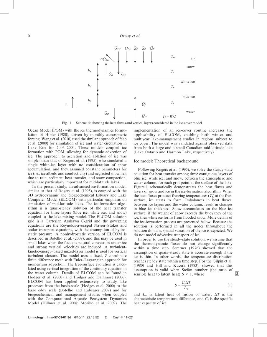
Following Rogers et al. (1995), we solve the steady-stateequation for heat transfer among three contiguous layers ofblue ice, white ice, and snow, between the atmosphere andwater column, for each grid point at the surface of the lake.Figure 1 schematically demonstrates the heat fluxes andlayers of snow and ice in the ice-formation algorithm. Whenthe heat fluxes produce freezing temperatures (Tf) at the free-surface, ice starts to form. Imbalances in heat fluxes,between ice layers and the water column, result in changesin blue ice thickness. Snow accumulates on the blue icesurface; if the weight of snow exceeds the buoyancy of theice, then white ice forms from flooded snow. More details ofthe ice-formation process are presented below. Because thesolution is performed in all the nodes throughout thesolution domain, spatial variation of the ice is expected. Wedo not model advective transport of ice.

In order to use the steady-state solution, we assume thatthe thermodynamic fluxes do not change significantlywithin a time step. Semtner (1976) showed that theassumption of quasi–steady state is accurate enough if theice is thin. In other words, the temperature distributionreaches steady state within a time step. For the Gilpin et al.(1980) and Hill and Kucera (1983), showed that thisassumption is valid when Stefan number (the ratio ofsensible heat to latent heat) S , 1, where =

S~CiDT

Lw

ð1Þ

and Lw is latent heat of fusion of water, DT is thecharacteristic temperature difference, and Ci is the specificheat capacity of ice.

Limnology limn-57-01-01.3d 6/10/11 22:13:52 2 Cust # 11-021

Fig. 1. Schematic showing the heat fluxes and vertical layers considered in the ice-cover model.

0 Oveisy et al.

With the assumption of equilibrium heat fluxes in eachtime step, we can ignore the term for rate of heat change. Inaddition, because we neglect advection within the ice andsnow cover, the steady-state heat conduction equation gives

kH

L2T

Lz2~

1

rncn

LQ

Lzð2Þ

where T is the temperature, Q is the heat flux, kH is the heatdiffusivity, rn is the snow or ice-cover density, cn is thespecific heat of snow or ice cover, and z is the verticalcoordinate.

Defining the thermal conductivity K 5 khrncn, thepenetrating radiation as

I~Isw exp {l h{zð Þ½ � ð3Þ

and considering the three distinct layers (i 5 blue ice, e 5white ice, and s 5 snow) in Fig. 1, yields

Ks

L2Ts

Lz2~A1ls1Isw exp {ls1 hizhezhs{zð Þ½ �

zA2ls2Isw exp {ls2 hizhezhs{zð Þ½ �zQsi~0,

hizhezhs§z§hizhe;

KeL2Te

Lz2~A1le1Isw exp {ls1hs{le1 hizhe{zð Þ½ �

zA2le2Isw exp {ls2hs{le2 hizhe{zð Þ½ �~0,

hizhe§z§hi;

Ki

L2Ti

Lz2~A1li1Isw exp {ls1hs{le1he{li1 hi{zð Þ½ �

zA2li2Isw exp {ls2hs{le2he{li2 hi{zð Þ½ �~0,

hi§z§0;

ð4Þ

where the incoming solar radiation Isw (Isw 5 1 2 aQsw,where a is the albedo at ice and snow cover) has beendivided into visible (subscript 1, A1 5 0.7) and near infra-red (subscript 2, A2 5 0.3) according to Kirk (1983) andBoer (1980), and a distinct attenuation coefficient l foreach component and ice and snow layer. Qsi is the heat fluxper volume released from white ice formation resultingfrom flooding of snow.

Temperature continuity and heat flux at interfaces of thelayers are

Ti~Tf ~0 z~0

Ti~Te

Ki

LTi

Lz~Ke

LTe

Lz

9=; z~hi

Te~Ts

Ks

LTs

Lz~Ki

LTi

Lz

9=; z~hi zhe

Ts~Ta z~hizhezhs ,

ð5Þ

where the indices f and a stand for freezing and air,respectively. Applying the boundary conditions in Eq. 5,the solution of Eq. 4 becomes

hs

Ks

zhe

Ke

zhi

Ki

� �Qo{Iswð Þ~ Tf {Ta

� �

{IswA1

1{ exp {ls1hsð ÞKsls1

z exp {ls1hsð Þ 1{ exp {le1heð ÞKele1

z exp {ls1hs{le1heð Þ 1{ exp {li1hið ÞKili1

26664

37775

{IswA2

1{ exp {ls2hsð ÞKsls2

z exp {ls2hsð Þ 1{ exp {le2heð ÞKele2

z exp {ls2hs{le2heð Þ 1{ exp {li2hið ÞKili2

26664

37775

zQsihs

hs

Ks

zhe

Ke

zhi

Ki

� �{

Qsih2s

2Ks

ð6Þ

With the value of heat flux at the air–ice or snow-coverinterface (Eq. 7) and water and blue-ice interface (Eqs. 8,9), Eq. 6 may be solved: >

QozQlwzQszQezQr~0; TavTf ~0oC

QozQlwzQszQezQr~rnLw

dhn

dt; Ta~Tf ~0oC

ð7Þ

Qf ~Qo{A1Isw 1{ exp { ls1hszle1hezli1hið Þ½ �f g{A2Isw 1{ exp { ls2hszle2hezli2hið Þ½ �f g{Qsihs

ð8Þ

Qw~{Kw

dTw

dzð9Þ

where Q0 is the incident solar radiation, Qlw is the net long-wave radiation, Qs is the sensible heat flux, Qe is the latentheat flux, and Qr is the heat flux due to rainfall. Parameter tis time and Lw is the latent heat of fusion of water. Qp ispenetrative solar radiation, Qf is the flux from ice to water,and Qw is the flux from water to the ice. Kw is the waterconductivity. Ice production and melting is the result ofimbalance between Qf and Qw. ?

dhi

dt~

Qf {Qw

riLw

ð10Þ

Implementation in ELCOM

Equations 1–10 were implemented in the ELCOMsurface-layer thermodynamics routine. To simulate thetemperature and ice cover in the two Canadian lakes duringwinter, the following process descriptions, relevant to mid-latitude lakes, were applied.

Limnology limn-57-01-01.3d 6/10/11 22:13:53 3 Cust # 11-021

Lake and ice dynamics during winter 0

Snow density—Snow can be flaky or watery, so itsdensity can vary significantly. Snow can also be signifi-cantly compacted over time. We consider snow densityvariable due to compaction (Koren et al. 1999).

rs,c~rs

exp (Bws){1

Bws

ð11Þ

where rs,c is the compacted snow density, ws is the waterequivalent in the snow, and B is calculated from

B~DtC1 exp (0:08Ts{C2rs) ð12Þ

where C1 5 2.77 3 1024 m21s21 and C2 5 0.021 m3 kg21.Unlike Rogers et al. (1995), who assumed constant densityof the fallen snow as 80 kg m23, the fallen snow densityis assumed to be a function of air temperature (Gottlieb1980).

rs,new~ max½50,1:7 Taz15ð Þ1:5� ð13Þ

and the average snow density was calculated from

rs~ min 400,rs,cws,czrs,newws,new

ws,czws,new

� �ð14Þ

where w refers to the relative water equivalent of the newfallen snow and the compacted snow, respectively.

Snow conductivity—Considerable increases in snowthermal conductivity may be expected when the snowdensity increases. The following equation (Ashton 1986)was used to describe the snow conductivity as the functionof the snow density:

Ks~0:021z4:2|10{3rsz2:2|10{9rs ð15Þ

Snow and ice albedo—Ice and snow may show a widerange of albedo (Henderson-Sellers 1984), which mainlydepends on the temperature of ice and snow and theirthicknesses. Variation of ice and snow albedo is particu-larly important at mid-latitude lakes where rapid weatherchanges are expected; observation shows the albedo of iceand snow decreases with increasing temperature. Thealbedo of snow and ice (as), (ai), respectively, were assumedvariable in this study and calculated as follows (Vavruset al. 1996):

Ice :

ai~0:6?Tsƒ{5oC

ai~0:44{0:032Ts?0oC§Ts§{5oC

ai~0:08{0:44hi0:28?

hiƒ0:5 m

hsƒ0:1 m

8>>><>>>:

; ð16Þ

Snow:

as~0:7?Tsƒ{5oC

as~0:50{0:04Ts?0oC§Ts§{5oC

as~as Tsð Þ{0:1{hi

0:1

� �as Tsð Þ{ai Ti,hið Þ½ �?

hiƒ0:5 m

hsƒ0:1 m

8>>><>>>:

ð17Þ

White ice—When the ice is not able to support theweight of accumulated snow, the snow layer becomesflooded. The thickness of the flooded snow layer may becalculated by comparing the thickness of snow (hs), to themaximum that can be supported by the existing blue ice(hs,max). A similar formulation as Rogers et al. (1995) wasused to calculate the formation of white ice (thickness he)and heat released (Qsi):

hs, max~hi rw{rið Þzhe rw{reð Þ

rs

ð18Þ

If hs . hs,max, we calculate increase of white ice thicknessand Qsi:

Dhe~hs{hs, max; ð19Þ

Qsi~

TwcazLf

� �rw

Dhe

hs

1{rs

rw

� �Dt

ð20Þ

then set hs 5 hs,max and he 5 he + Dhe.

Rain—In high-latitude lakes, it is rare to observe meltingof snow by rain due to the very small chance of rain duringthe freezing season and also because of the sub-freezingtemperature of snow (Parkinson and Washington 1979;Patterson and Hamblin 1988). However, in mid-latitudelakes it is not unusual to have frequent rain on top ofpreviously fallen snow. The heat may increase thetemperature and so result in melting. We calculate heatflux released from the rain to the snowpack by eithersensible transfer or due to rain freezing as follows:

Qr~caro Ta{Tsð ÞR?Ts~0oC

Lf roR?Tsv0oC

�ð21Þ

where R is the amount and ca the heat capacity of rain,respectively.

The model parameters used in this study are presented inTable 1.

Validation of the ice and snow model

The ice-formation model as described above wasimplemented in ELCOM and then validated against

Limnology limn-57-01-01.3d 6/10/11 22:13:53 4 Cust # 11-021

Table 1. Parameters used in the ice and snow model (Rogerset al. 1995).

Parameter Value

Ice visible solar attenuation coefficients (m21) 6.00Snow visible solar attenuation coefficients (m21) 1.50White-ice visible solar attenuation coefficients (m21) 3.75Ice infrared solar attenuation coefficients (m21) 20.0Snow infrared solar attenuation coefficients (m21) 20.0White-ice infrared solar attenuation coefficients (m21) 20.0Conductivity of blue ice (W m21 uC21) 2.00Conductivity of white ice (W m21 uC21) 2.30Specific heat of ice (kJ kg21 uC21) 2.10Latent heat of fusion (kJ kg21) 334Blue-ice density (kg m23) 917

0 Oveisy et al.

observed data from a winter season in Lake Ontario (43.63N, 77.92 W) and Harmon Lake (49.97 N, 120.70 W). Theselakes were selected to test the performance of the modelbecause they represent two extreme lake sizes and also havedifferent space–time ice-cover characteristics.

Lake Ontario has approximate dimensions of 300 km 3120 km and a maximum depth of 250 m (Fig. 2).Themaximum extent of lake ice is typically , 20% of thesurface area, mostly at the shallow northeast end (KingstonBasin) where heat storage is minimal. Previous multiyearsimulations of Lake Ontario, using an unstructured gridFinite Volume Coastal Ocean Model that neglected winterice effects (Shore 2009), showed an , 2uC overestimationof spring water temperature (Wang et al. 2010).@

Harmon Lake is a small sheltered lake in BritishColumbia, which is , 1200 m 3 275 m with a maximumdepth of 22 m (Fig. 3). The entire surface of Harmon Laketypically freezes during winter.

Following Wang et al. (2010), we quantify the capabilityof the model using the statistical measures of Mean BiasDeviation (MBD) and Root Mean Square Deviation(RMSD):

MBD~100

1

N

XN

i~1

xi{yið Þ

1

N

XN

i~1

yi

; ð22Þ

RMSD~1

N

XN

i~1

xi{yið Þ2" #1=2

ð23Þ

where xi and yi (i 5 1,2,3,..N) are the model and observedvariable time-series, respectively, and N is the total numberof samples. MBD, which characterizes the bias of a model,is negative or positive if the model, respectively, under-predicts or over-predicts a variable. RMSD is the absoluteerror of the model against the observation.

Application to Lake Ontario

Model setup—The winter season of 2006–2007 wasselected because ELCOM had already been used toaccurately model the ice-free period (spring through autumn)of 2006 (Hall 2008; Boegman and Rao 2010). The model wasinitialized from rest on day 284 of 2006, with initial valuestaken from four in-lake measurement stations (Fig. 2) andinterpolated throughout the domain using inverse distancemethods, and was run until day 120 of 2007, a total of 201 d.The horizontal grid spacing was 2 km 3 2 km and the modelhad 54 vertical layers, varying from 0.25 m near the surface to16 m at the lake bed. Because Environment Canadamoorings are removed from the lake during the ice-cover

Limnology limn-57-01-01.3d 6/10/11 22:13:53 5 Cust # 11-021

Fig. 2. Map of Lake Ontario bathymetry. Stations identified with an asterisk (IV4, 403, 586, and 1263) were used for thetemperature profile initial condition. Stations identified with open circles were used for SST extraction points (Fig. 6). Filled circles showthe locations of the Lake Ontario vertical temperature profile measurements that are compared with simulations results in Fig. 7.

Fig. 3. Map of Harmon Lake bathymetry and location ofmeasurement marked with an open circle.

Lake and ice dynamics during winter 0

season, for validation purposes the run period was chosen tooverlap with the end of the 2006 measurement period and thebeginning of the 2007 field season. The driving meteorolog-ical forces are from land stations at Hamilton (BurlingtonPier, Environment Canada) and Kingston (Queen’s Univer-sity Integrated Learning Centre) and were interpolated onto

158 surface zones using an inverse distance methodthroughout the simulation domain. The wind velocities fromland stations were first adjusted (mean and standarddeviation) for the differences between over-land and over-lake conditions, through comparison of land data to over-lake data (Sta. 1263 and Sta. 403; Fig. 2).

Limnology limn-57-01-01.3d 6/10/11 22:13:54 6 Cust # 11-021

Fig. 4. Comparison of modeled and satellite-observed ice thickness on Lake Ontario during winter 2006–2007. Contour intervalswere specified according to the satellite data.

0 Oveisy et al.

During the ice-free portion of 2006 the input data for thesimulation were wind velocity, air temperature, relativehumidity, shortwave solar radiation, and lake-averageprecipitation. When the air temperature drops belowfreezing, the model interprets precipitation as snow withthe associated density calculated by Eq. 13. The long-waveradiation was calculated in the model based on the differencebetween observed and clear-sky shortwave radiation.

We follow Patterson and Hamblin (1988) and define aminimum ice thickness of 0.1 m. Accurate determination ofice thicknesses near this limiting value remains a challengingproblem in the current implementation. The ice dynamics atthis limit are regulated by processes we do not model,including wind-induced turbulence, surface wave action, andunderflow beneath the ice. Ice formed at thicknesses lessthan this value will be readily broken up by surface processesand advected. However, to account for broken ice, when theice thickness is less than the minimum thickness, the modelstill uses the ice thickness in flux calculations.

Simulation results—The simulation results for ice thick-ness were compared against the Canadian Ice Services icecharts derived from satellite imagery (Nghiem and Leshke-vich 2007). In general, the spatial pattern of ice formationand its temporal evolution is in favorable qualitativeagreement with the observations (Fig. 4). There is greaterspatial ice coverage in the observations during winter, butthe observed ice is thinner than modeled. During spring,the observed and modeled ice has nearly identical spatialcoverage and similar thicknesses. Errors in thickness mayresult from the model simulating both blue and white ice;whereas in the observations, these ice types are aggregated.Moreover, the satellite-derived ice-thickness observationspresented in this study have not been ground-verifiedagainst direct ice-thickness measurements. Ice mostly formsin the northeast portion and marginally in the southwest ofthe lake, which is consistent with the observations. Lowerwater temperatures are associated with the smaller heatstorage in the shallow-water depths in these regions and sofavor ice formation. Persistent ice coverage also occurs inthe shallow area along the north shore. In Fig. 5, themodeled ice coverage is reported as a percentage of the lakesurface and it is within 5% of the observed value. In thisfigure, the volume of ice divided by the lake surface area isalso presented, which is within 1.5 cm of the observation.

In addition to errors in ice observation, the discrepanciesin Figs. 4 and 5 might be due to several other factors. Inlarge lakes, ice drift is significant in the early periods of iceformation and the lack of advective ice dynamics in the ice-formation model could lead to errors in simulation becauseice could be transported by wind and hydrodynamic forces.For example, comparison of the ice charts on 15 Marchand 02 April shows increases in the ice thickness near shore,while the ice is disappearing in deeper parts of the lake. Thereasons for this process may be due to ice transport by thewind toward nearshore areas. The other factor thatcontributes to the discrepancies may be the rather large2-km horizontal grid in resolving bathymetry in nearshoreregions—in particular, near the Kingston Basin where thereare numerous islands and lakebed channels.

Ideally, such a large domain needs to be forced usingspatially accurate metrological data. Inclusion of data froma third land station at Oswego, New York resulted in thepattern of ice formation being significantly different fromobservations and increased ice coverage in the south andsoutheast of the lake. This undesirable pattern could be dueto the quality of data at this station, or the relevancy of thedata for over-lake metrological forcing. Therefore, specialcare has to be taken in choosing and correcting metrolog-ical data, and the model must be validated againstobservations to ensure deficiencies in winter meteorologicalforcing are not leading to erroneous results.

Better estimation of the model parameters for a specificlake could result in better ice-thickness prediction, because theresults were highly sensitive to the input parameters. Forexample, the albedo of snow significantly changes, from 0.95for freshly fallen snow to 0.2 for slushy, gray, melting snow(Henderson-Sellers 1984). Choosing the wrong value cansignificantly affect the heat reception of the lake. The modeledlake temperatures were validated against satellite-derived seasurface temperatures (SST) at 11 locations (Fig. 2) in the lakeduring the winter of 2006–2007 (Fig. 6). In-situ mooring datawere not available during this period because moorings areremoved during the winter ice season. The observationtemperature is based on satellite imagery and was providedby Great Lakes Environmental Research Laboratory ofNational Oceanic and Atmospheric Administration; themodeling results follow the observation with few discrepan-cies, the average MBD and RMSD for all the locations shownare 22.5% and 1.0uC, respectively, showing that the modelslightly under-predicts the SST. Cyclic variation of airtemperature, resulting from atmospheric storm-front activity

Limnology limn-57-01-01.3d 6/10/11 22:13:59 7 Cust # 11-021

Fig. 5. Quantitative comparison of modeled and observedice distributions. (a) Total volume of ice divided by the surfacearea of the lake in (cm), and (b) percentage of the lake surfacecovered with ice.

Lake and ice dynamics during winter 0

with a 10-d period (Hamblin 1987) can be seen in the observedand simulated SST. At point P1 in Fig. 2, for the majority oftime the SST is close to zero because it is under ice cover; thetemperature increases in spring when the ice cover melts.A

ELCOM also reproduced the vertical profiles of watertemperature at six stations (Fig. 2) on day 106 of 2007. Themodel shows agreement with the temperature profiles at allstations with , 1uC difference (Fig. 7). The model error willbe partially a result of the coarse 2-km gridding not resolvingnearshore temperature patchiness and small-scale topograph-

ic features. The water column was below the temperature ofmaximum density of 4uC, causing both modeled andobserved profiles to exhibit reverse winter stratification, withtemperatures decreasing toward the surface.

Modeled contours of temperature profiles at P12 andP13 (Fig. 2) show the differences in water-column dynam-ics occurring as a function of depth (Fig. 8). The relativelyshallow water column (, 25-m depth) at P12 cooled muchfaster than the deeper water (, 50-m depth) at P13, afterthe autumn turnover; P12 then experienced a significant

Limnology limn-57-01-01.3d 6/10/11 22:14:00 8 Cust # 11-021

Fig. 6. Comparison of modeled and observed sea surface temperature (SST). Observations are derived from satellite observations.Locations of comparisons are indicated on Fig. 2.

0 Oveisy et al.

period of ice cover and zero surface temperatures. Thestrong sheltering effect of the ice is seen clearly byobserving the modeled rate of dissipation of turbulentkinetic energy for this period, at P13 relative to P12, whereno ice cover was predicted by the model and temperaturesremained above freezing (Fig. 9). At P13, dissipation wasreduced where the water column remains weakly stratified.At both stations the reverse winter stratification, springturnover, and onset of seasonal stratification are clearlyrecognizable. These comparisons confirm that good pre-dictions of both the surface and the vertical temperature

conditions may be achieved from autumn to the start of thespring season. Because ELCOM has been shown to modelaccurately the Lake Ontario thermal structure and hydro-dynamics from spring turnover through autumn turnoverduring 2006 (Hall 2008; Boegman and Rao 2010), themodel is now capable of year-round simulation.

Application to Harmon Lake

Model setup—The winter season from the 13 December1991 to 24 March 1992 was chosen to model Harmon Lake

Limnology limn-57-01-01.3d 6/10/11 22:14:00 9 Cust # 11-021

Fig. 7. Vertical profiles of temperature (Temp) on day 106 of 2007 at time 00:00 h. Thelocations of the profiles are shown in Fig. 2. The measurements were taken using Tidbit loggersthat have an accuracy of 6 0.2uC.

Lake and ice dynamics during winter 0

Limnology limn-57-01-01.3d 6/10/11 22:14:00 10 Cust # 11-021

Fig. 8. Contours of modeled temperature time-series (uC) under (a) ice-covered, and (b) ice-free stations in the Kingston Basin ofLake Ontario. Sta. (a) P12, and (b) P13 are indicated on Fig. 2. Note the different vertical scales. The black line above panel denotes theperiod of ice cover.

Fig. 9. Depth vs. time contours of modeled dissipation of turbulent kinetic energy (log10 dissipation) in Lake Ontario at Sta. (a) P12,and (b) P13. Note the different vertical scales. The black line above panel indicates the period of ice cover.

0 Oveisy et al.

because data were available for this period (Rogers et al.1995): in general, there exist very little data (e.g., ground-measured ice and snow thickness and lake temperature)from ice-covered lakes (Bengtsson 1996).

A 50-m 3 50-m horizontal grid was applied with 53vertical layers, ranging from 0.25 m at the surface to 0.5 mnear the bed. Meteorological data (including solar radia-tion, wind speed, relative humidity, and air temperature

[Fig. 10] for this simulation), as reported in Rogers et al.(1995), were measured at Menzies Lake, about 5 kmnortheast of Harmon Lake and 100 m higher in elevation.Rainfall was measured at Merritt, 15 km northwest ofHarmon Lake, and snowfall was measured using snow-board observations (accuracy . 6 1 cm) after each snowevent. Wind direction was not reported in Rogers et al.(1995), because their 1D vertical model does not require

Limnology limn-57-01-01.3d 6/10/11 22:14:06 11 Cust # 11-021

Fig. 10. Meteorological data collected at Menzies Lake, 13 December 1991–27 March 1992. Rain values are from Merritt, which islocated 15 km northwest of Harmon Lake. Data have been digitally reconstructed from Rogers et al. (1995).

Lake and ice dynamics during winter 0

this input. We used wind direction from metrologicalstation at Merritt. In the specific case of modeling HarmonLake, the lake was ice covered during whole simulation andwind had no drag forces on the water surface; therefore,direction of wind does not have any significant effect on theoutcome of the model.

Ice and snow thickness (there was no distinction betweenblue ice and white ice) were measured during several fieldtrips to Harmon Lake at the deepest part of the lake(Fig. 3). Vertical profiles of water temperature were alsomeasured at the same location. Because much compactioncan take place over the first 24 h following a snowfall, andbecause the snow boards may not have been ideally placedwith respect to exposure, the errors in estimating the actualdepth of snowfall are probably much greater (Rogers1992). Because of potential inaccuracies in precipitationmeasurements, relative to local conditions and the stronginfluence of precipitation on ice formation, the observedsnow and rainfall values (Fig. 10) were compared with thesnow-thickness observations at Harmon Lake (Fig. 10) inorder to make any necessary adjustments. The snowfallswere found to be much higher than the increase in snowdepth; for example, from 15 January to 19 January about19 cm of snow was measured and during this period the airtemperature was significantly below freezing, but snowthickness on 19 January was about 7 cm and was actuallyless than the depth of snow on 14 January. Althoughsignificant snow compaction was not expected for thisperiod, snow transport could be one of the reasons forthese differences (Rogers et al. 1995). For adjustment, usingobserved snow depths, we assumed one-third of theobserved snowfall at Menzies Lake for modeling ofHarmon Lake. In addition, the precipitation was adjustedbased on air temperature: when the air temperature wasabove or below the freezing point, the precipitation was

converted to rain or snow, respectively. The model wasinitialized on 13 December 1991, with observed initialconditions of snow and ice thicknesses of 14 cm and 12 cm,respectively (Fig. 11). There was assumed to be no whitesnow as an initial condition, because the initial ice thicknesscould tolerate the initial weight of the snow on top of it.The initial condition for water temperature was themeasured vertical profile of temperature on 13 December(Fig. 12). Rates of sediment heat transfer at both mid- andhigh-latitude lakes during ice-covered periods are typicallyin the range of 1–5 Wm22 (Birge et al. 1927; Likens andJohnson 1969; Ashton 1986), considering sediment heatfluxes can contribute to internal mixing, particularly insmall lakes (Mortimer and Mackereth 1958; Welch andBergmann 1985). In this simulation, 1 Wm22 is assumed forheat release from sediment to the lake. We assumed 0.02 forthe albedo of ice (Rogers et al. 1995).

Simulation results—As seen in Fig. 11 for the first 80 d,the ice thickness increased from , 0.15 m to 0.35 m over,the simulations closely following the observations. Theincrease in thickness resulted from below-freezing airtemperatures and low-incident shortwave radiation char-acteristic of winter conditions (Fig. 10). The initial snowthickness on top of the ice first decreased due tocompaction (to day 23), then increased with increasingsnowfall (day 25 to day 38), but this melted to a near-zerothickness, due to significant rainfall (Fig. 11, day 50;Fig. 10, 20 Jan). Coupling between ice and snow isillustrated by the model results; the heavy snow (Fig. 11,days 30–40; Fig. 10, 30 Dec–19 Jan) acted to insulate theice and slowly increased in ice thickness during this time.The ability of the model to capture these rapid responses ofsnow and ice dynamics to daily changes in meteorologicalconditions emphasizes the importance of implementing

Limnology limn-57-01-01.3d 6/10/11 22:14:07 12 Cust # 11-021

Fig. 11. Comparison of modeled and observed ice and snow thicknesses at Harmon Lakeduring 1991–1992. Modeled time-series are daily output from the present study and results fromthe MLI model (Rogers et al. 1995). The less frequent observations are described fully in the text.

0 Oveisy et al.

snow- and ice-melting due to rain in the ice algorithm.Toward the end of the simulation, the air temperaturesincreased above freezing and solar radiation also increased(Fig. 10) leading to a decrease in ice thickness. In Fig. 11,the MLI modeling result is also presented. The mainreasons for the better performance of ELCOM, comparedto MLI are the one-dimensional nature of MLI, whichneglects water-column dynamics beneath the ice and thesimplified prediction of water surface temperature as afunction of solar radiation reaching the water in MLI.

A comparison between observations and simulationresults of the vertical profile of temperature, at the deepestpart of the lake, is shown in Fig. 12; in general, thecomparisons are excellent. The reverse winter stratificationis well-modeled, with colder water overlying warmer waterapproaching 4uC near the lake bed. The surface waterswarmed up a little later in the model in spring than theobservations suggest, but for the remainder of the simulationperiod the comparisons are excellent. Convective mixingevents, associated with warming of the water column, actingto homogenize the water column and deepen the stratifica-tion from 15 m to 22 m (Fig. 13), are simulated to occur withturbulent dissipation rates of 1026–1027 m2 s23. At othertimes, beneath the ice, dissipation remained negligible.

Discussion

The model results may be compared with data from otherobservational studies. The sharp temperature gradientimmediately beneath the ice (Fig. 12) is characteristic ofother small lakes (Bengtsson 1996; Forrest et al. 2008), as isthe reverse stratification occurring beneath ice cover (Farmerand ESCarmak 1981). Similar observations do not exist forother Great Lakes. However, in the shallow nearshore ice-covered regions, of Lake Ontario, the modeled water-columndynamics are analogous to small lake systems (Fig. 8a).

The accuracy of the predictions for Lake Ontario may becompared to those reported by Wang et al. (2010) in theirmodel application to Lake Erie. Both modeling effortsreasonably predict SST (present: MBD 5 22.5% and

Limnology limn-57-01-01.3d 6/10/11 22:14:07 13 Cust # 11-021

Fig. 12. Contours of modeled and observed water-columntemperature in depth vs. time space for Harmon Lake. Isothermshave been computed by linearly interpolating model output atdiscrete depths. The observed data were digitally reconstructedfrom Rogers et al. (1995), and the crosses indicate the days whenvertical profiles of temperature were measured. The isothermsbelow 3uC are not shown on the figure for clarity of presentation.The entire period shown is ice-covered.

Fig. 13. Depth vs. time contours of modeled dissipation of turbulent kinetic energy (log10 dissipation) in Harmon Lake during 1991–1992. The lake is ice covered throughout the entire simulation.

Lake and ice dynamics during winter 0

RMSD 5 1.0uC; Wang et al. [2010]: MBD 5 1.5% andRMSD 5 1.0uC). Ice-cover simulations (ice volume andsurface area) are also similar (present model: MBD 521.9% and RMSD 5 1.4 cm; Wang et al. [2010]: MBD 57.4% and RMSD 5 1.84 cm), showing that including theprocess of ice advection does not lead to improvements inthe overall prediction of ice-cover characteristics, althoughice advection is likely important in the spatial patterns of icecoverage in large lakes during partial ice cover. The lack ofobservational data on ice thickness and low accuracy of theice data extracted from satellite imagery makes furtherverification of the models difficult. The ice cover isolates thelake from the air; however, other mechanisms such as wind-induced oscillation of the ice cover can generate seiches andenhance mixing. Although very little observational data existto quantify this process, the horizontal mixing coefficientscould be in the other of 100 cm22 s21 (Bengtsson 1996). Suchmechanisms are neglected in this study.B

In the winter season, physical observations of lakehydrodynamics under ice cover are difficult (Forrest et al.2008) and infrequent (Mortimer and Mackereth 1958;Farmer and Carmack 1981). Using ELCOM with the ice-formation capability, we can better investigate winter lakeprocesses that ultimately influence biogeochemistry, suchas thermal bar and inverse winter stratification. Studies onfundamental limnology and source-water management, incold climates, may be more easily extended through thewinter, and ELCOM can be used for multiyear climate-change–coupled atmosphere–lake modeling (Leon et al.2007).

A three-component ice-formation algorithm for blue ice,with ice and snow, has been added to ELCOM, extendingthe capability of the model for full-year simulations inregions that experience seasonal ice cover. Unlike previouslake-ice applications, the model allowed for significantvariation of parameters (e.g., albedo, snow density) overshort timescales, as is expected in mid-latitudes, andcoupling to a three-dimensional hydrodynamic lake modelprovided the temporal and spatial variability needed tosimulate lake biogeochemistry. The model was validatedagainst observed data from both small and large Canadianlakes located in mid-latitude modeled temperatures; thepercentage of lake surface covered with ice and the icethickness were typically within 1uC, 5%, and 2 cm ofobservations, respectively. The evolution of the thermalstructure from reverse winter stratification through springturnover was also correctly simulated. The model washighly sensitive to the snow and ice parameters; furtherresearch on quantitative physical observation of ice cover isessential for improved numerical simulation.

AcknowledgmentsDaniel Botelho performed the initial implementation of the

Rogers et al. (1995) ice model into Estuary and Lake ComputerModel (ELCOM). We acknowledge funding from the Environ-ment Canada Lake Simcoe Cleanup Fund, Queen’s University,and the Western Australian Water Corporation. The LakeOntario temperature profile data and the Burlington meteorolog-ical data was provided by Ram Yerubandi at the National WaterResearch Institute, Environment Canada. The Lake Ontarioprecipitation data was provided by Tim Hunter at National

Oceanic and Atmospheric Administration and the Sea SurfaceTemperature data by George Leshkevich at National Oceanic andAtmospheric Administration, Great Lakes Environmental Re-search Laboratory. We also would like to thank the reviewers ofthis manuscript for their insight and suggestions. This paper formsCenter for Water Research reference 2384.

References

ASHTON, G. D. [ED.]. 1986. River and lake ice engineering. WaterResources.

BENGTSSON, L. 1996. Mixing in ice-covered lakes. Hydrobiologia322: 91–97, doi:10.1007/BF00031811

BOEGMAN, L., AND R. YERUBANDI RAO. 2010. Process orientedmodeling of Lake Ontario hydrodynamics, p. 1–6. In G. C.Christodoulou and A. I. Stamou [eds.], Proceedings 6thInternational Symposium on Environmental Hydraulics. C

BOTELHO, D., AND J. IMBERGER. 2007. Down-scaling modelresolution to illuminate the internal wave field in a smallstratified lake. J. Hydraul. Eng.-ASCE 133: 1206–1218,doi:10.1061/(ASCE)0733-9429(2007)133:11(1206)

———, ———, C. DALLIMORE, AND B. R. HODGES. 2009. Ahydrostatic/non-hydrostatic grid-switching strategy for com-puting high-frequency, high wave number motions embeddedin geophysical flows. Environ. Modell. Softw. 24: 473–488,doi:10.1016/j.envsoft.2008.09.008

BIRGE, E. A., C. JUDAY, AND H. W. MARCH. 1927. The temperatureof the bottom deposits of Lake Mendota; a chapter in the heatexchanges of the lake. Trans. Wis. Acad. Sci. 23: 187–231.

BOER, K. W. 1980. The terrestrial solar spectrum, p. 65–87. InW. C. Dickinson and P. N. Chercmisinoff [eds.], Solar energytechnology handbook, part A. Dekker.

CHAPRA, S. C. [ED.]. 1986. Surface water-quality modeling. WCB/McGraw-Hill.

FARMER, D. M. 1975. Potential temperatures in deep freshwaterlakes. Limnol. Oceanogr. 20: 634–635, doi:10.4319/lo.1975.20.4.0634

———, AND E. CARMACK. 1981. Wind mixing and re-stratificationin a lake near the temperature of maximum density. J. Phys.Oceanogr. 11: 1516–1533, doi:10.1175/1520-0485(1981)011,1516:WMARIA.2.0.CO;2

FORREST, A. L., B. E. LAVAL, R. PETERS, AND D. S. S. LIM. 2008.Convectively driven transport in temperate lakes. Limnol.Oceanogr. 53: 2321–2332, doi:10.4319/lo.2008.53.5_part_2.2321

GILPIN, R. R., T. HIRATA, AND K. C. CHENG. 1980. Waveformation and heat transfer at an ice-water interface inthe presence of a turbulent flow. J. Fluid Mech. 99: 619–640,doi:10.1017/S0022112080000791

GOSINK, J. P. 1987. Northern lake and reservoir modeling. ColdRegions Science and Technology 13: 281–300, doi:10.1016/0165-232X(87)90008-5

GOTTLIEB, L. 1980. Development and applications of a runoffmodel for snow covered and glacierized basins. Nord. Hydrol.11: 255–272.

HALL, E. 2008. Hydrodynamic modeling of Lake Ontario. M.Eng. thesis. Queen’s Univ.

HAMILTON, D. P., C. M. SPILLMAN, K. L. PRESCOTT, T. K. KRATZ,AND J. J. MAGNUSON. 2002. Effects of atmospheric nutrientinputs and climate change on the trophic status of CrystalLake, Wisconsin. Verh. Int. Verein. Limnol. 28: 467–470.

HENDERSON-SELLERS, B. 1984. Engineering limnology. Pitman.———. 1986. Calculating the surface energy balance for lake and

reservoir modeling: A review. Rev. Geophys. 24: 625–649 EX,doi:10.1029/RG024i003p00625

Limnology limn-57-01-01.3d 6/10/11 22:14:09 14 Cust # 11-021

0 Oveisy et al.

HIBLER, W. D. 1980. Modeling a variable thickness sea ice cover.Mon. Weather Rev. 108: 1943–1973, doi:10.1175/1520-0493(1980)108,1943:MAVTSI.2.0.CO;2

HILL, J. M., AND A. KUCERA. 1983. Freezing a saturated liquidinside a sphere. Int. J. Heat Mass Tran. 26: 1631–1638,doi:10.1016/S0017-9310(83)80083-0

HILLMER, I. A., P. VAN REENEN, J. IMBERGER, AND T. ZOHARY.2008. Phytoplankton patchiness and their role in the modeledproductivity of a large, seasonally stratified lake. Ecol. Model.218: 49–59, doi:10.1016/j.ecolmodel.2008.06.017

HODGES, B. R. 2009. Hydrodynamical modeling, p. 613–627. InG. E. Likens [ed.], Encyclopedia of inland waters. Elsevier.

———, AND C. DALLIMORE. 2006. Estuary, lake and coastal oceanmodel: ELCOM science manual report. Perth, Western Australia:Centre for Water Research, University of Western, Australia;[accessed year month day]. Available from www.cwr.uwa.edu.au/…/models/elcom2/…/elcom_science…/ELCOM_Science.pdf.EO

———, J. IMBERGER, A. SAGGIO, AND K. B. WINTERS. 2000.Modeling basin-scale internal waves in a stratified lake, J.Limnol. Oceanogr. 45: 1603–1620.

IKEDA, M., T. YAO, AND Q. YAO. 1996. Seasonal evolution of seaice cover and shelf water off Labrador simulated in a coupledice–ocean model. J. Geophys. Res. 101: 465–489EP , doi:10.1029/96JC00716

KIRK, J. T. O. 1983. Light and photosynthesis in aquaticecosystems. Cambridge Press.

KOREN, V., J. SCHAAKE, K. MITCHELL, Q. Y. DUAN, F. CHEN, AND J.M. BAKER. 1999. A parameterization of snowpack and frozenground intended for NCEP weather and climate models. J.Geophys. Res. 104: 19569–19585, doi:10.1029/1999JD900232

LEON, L. F., D. C.-L. LAM, W. M. SCHERTZER, D. SWAYNE, AND J.IMBERGER. 2007. Towards coupling a 3D hydrodynamic lakemodel with the Canadian Regional Climate Model: Simula-tion on Great Slave Lake. Environ. Modell. Softw. 22:787–796, doi:10.1016/j.envsoft.2006.03.005

LIKENS, G. E., AND N. M. JOHNSON. 1969. Measurement andanalysis of the annual heat budget for the sediments in twoWisconsin lakes. Limnol. Oceanogr. 14: 115–135, doi:10.4319/lo.1969.14.1.0115

MAYKUT, G. A., AND N. UNTERSTEINER. 1971. Some results from atime-dependent Thermodynamic model of sea ice. J. Geophys.Res. 76: 1550–1575, doi:10.1029/JC076i006p01550

MCCORD, S. A., S. G. SCHLADOW, AND T. G. MILLER. 2000.Modeling artificial aeration kinetics in ice covered lakes. J.Environ. Eng.-ASCE. 126: 21–31, doi:10.1061/(ASCE)0733-9372(2000)126:1(21)

MORILLO, S., J. IMBERGER, J. P. ANTENUCCI, AND D. COPETTI. 2009.Using impellers to distribute local nutrient loadings in astratified lake; Lake Como, Italy. J. Hydraul. Eng.-ASCE135: 564–574, doi:10.1061/(ASCE)HY.1943-7900.0000048

MORTIMER, C. H., AND F. J. H. MACKERETH. 1958. Convectionand its consequences in ice-covered lakes. Verh. Int. Verein.Theor. Angew. Limnol. 13: 923–932.

NGHIEM, S. V., AND G. A. LESHKEVICH. 2007. Satellite SAR remotesensing of Great Lakes ice cover. Part 1. Ice backscattersignatures at C band. J. Great Lakes Res. 33: 722–735,doi:10.3394/0380-1330(2007)33[722:SSRSOG]2.0.CO;2

PARKINSON, C., AND W. WASHINGTON. 1979. A large-scalenumerical model of sea ice. J. Geophys. Res. 84: 311–337,doi:10.1029/JC084iC01p00311

PATTERSON, J. C., AND P. F. HAMBLIN. 1988. Thermal simulation ofa lake with winter ice cover. Limnol. Oceanogr. 33: 323–338,doi:10.4319/lo.1988.33.3.0323

ROGERS, C. K. 1992. Impact of an artificial circulation device onthe heat budget of an ice-covered mid-latitude lake. M.S.thesis, Univ. British Columbia.

———, G. LAWRENCE, AND P. F. HAMBLIN. 1995. Observationsand numerical simulation of a shallow ice-covered mid-latitude lake. Limnol. Oceanogr. 40: 374–385, doi:10.4319/lo.1995.40.2.0374

RUMER, R. R., A. WAKE, AND S. H. SHIEH. 1981. Development ofan ice dynamics forecasting model for Lake Erie researchreport No. 81-1. Buffalo (NY): Department of CivilEngineering, Center for Cold Regions Science and Technol-ogy, State University of New York at Buffalo.

SEMTNER, A. J. 1976. A model for thermodynamic growth of sea icein numerical investigations of climate. J. Phys. Oceanogr. 6:379–389, doi:10.1175/1520-0485(1976)006,0379:AMFTTG.2.0.CO;2

SHORE, J. 2009. Modeling the circulation and exchange ofKingston Basin and Lake Ontario with FVCOM. OceanModell. 30: 106–114, doi:10.1016/j.ocemod.2009.06.007

VAVRUS, S. J., R. H. WYNNE, AND J. A. FOLEY. 1996. Measuringthe sensitivity of southern Wisconsin lake ice to climatevariations and lake depth using a numerical model. Limnol.Oceanogr. 41: 822–831, doi:10.4319/lo.1996.41.5.0822

WAKE, A., AND R. R. RUMER. 1979. Modeling the ice regime ofLake Erie. J. Hydraul. Eng.-ASCE 105: 827–844.

WANG, J., H. HU, D. SCHWAB, D. BELETSKY, A. CLITES, AND G.LESHKEVICH. 2010. Development of the Great Lakes ice-circulation model (GLIM): Application to Lake Erie in 2003–2004. J. Great Lake Res. 36: 425–436, doi:10.1016/j.jglr.2010.04.002

WELCH, H. E., AND M. BERGMANN. 1985. Water circulation insmall arctic lakes in winter. Can. J. Fish. Aquat. Sci. 42:506–520, doi:10.1139/f85-068

YAO, T., C. L. TANG, AND I. K. PETERSON. 2000. Modeling theseasonal variation of sea ice in the Labrador Sea with a coupledmulticategory ice model and the Princeton ocean model. J.Geophys. Res. 105: 1153–1165, doi:10.1029/1999JC900264

Associate editor: Chris Rehmann

Received: 12 January 2011Accepted: 24 August 2011

Amended: 15 September 2011

Limnology limn-57-01-01.3d 6/10/11 22:14:10 15 Cust # 11-021

Lake and ice dynamics during winter 0