Embed Size (px)
Citation preview
Three Essays on the Estimation of Chinese Textile Demand and Its
Implications for the World Cotton Market
by
Mouze M.Kebede
A Dissertation
In
AGRICULTURE AND APPLIED ECONOMICS
Submitted to the Graduate Faculty
of Texas Tech University in
Partial Fulfillment of
the Requirements for
the Degree of
DOCTOR OF PHILOSOPHY
Approved
Dr. Darren Hudson
Chair of Committee
Dr. Dean Ethridge
Dr. Benaissa Chidmi
Dr. Eric Walden
Peggy Gordon Miller
Dean of the Graduate School
August, 2012

©2012, Mouze Mulugeta Kebede

Texas Tech University, Mouze Mulugeta Kebede, August 2012
ii
Acknowledgments
My special thanks and appreciation goes to those who have made this work a lot
easier to complete than what would have been needed. A special word of appreciation
goes to my major advisor, Dr. Darren Hudson, for his constructive comments, support,
patience, and guidance during this research work. My special appreciation also goes to
my dissertation committee, Dr. Dean Ethridge, Dr. Benaissa Chidmi, Dr. Suwen Pan, and
Dr. Eric Walden who have been patient and constructive in this research. Their constant
support has made this work a success.
I would like to thank Cotton Council International (CCI) who provided the data and
USDA/ERS and CERI for providing financial support for this research. I would also like
to extend my thanks to the faculty, staff, and students of the Department of Agricultural
and Applied Economics at Texas Tech which have made my stay at Texas Tech easy, and
a lot enjoyable.
My special thanks also go to my family members in Ethiopia, especially, my father,
Mulugeta, my mother, Neber, and my siblings for their constant encouragement, support
and prayer during this research work.
Texas Tech University, Mouze Mulugeta Kebede, August 2012
iii
Table of Contents
Acknowledgements………………………………………………………………………ii
Abstract…………………………………………………………………………………..v
List of Tables……………………………………………………………………………viii
List of Figures……………………………………………………………........................ix
Chapter
Chapter one………………………………………………………………………………..1
Introduction .................................................................................................................................. 1
1.1 Changes in Chinese Demographic Structure ......................................................................... 4
1.2 Changes in Shopping Habits of Chinese Households ............................................................. 6
1.3 Specific Problem .................................................................................................................... 8
1.5 Objectives of the Study .......................................................................................................... 9
Chapter Two .................................................................................................................................. 10
Review of Literature ...................................................................................................................... 10
2.1 Review of Demand Functional Forms ................................................................................. 10
2.2 Review of Empirical Literature on Textile Demand ............................................................ 19
2.3. Review of the Global Fiber Model ..................................................................................... 25
Chapter Three ................................................................................................................................ 10
Choice of Retail Outlets and Chinese Household Demand for Textiles and Footwear: Analysis
Using Alternative Demand Functional Forms ............................................................................... 29
Introduction ................................................................................................................................ 29
3.1 Conceptual Framework ........................................................................................................ 30
3.2 Methods and Procedures ...................................................................................................... 32
3.3 Data Source and Description ............................................................................................... 39
3.4 Results and Discussion ........................................................................................................ 44
3.4.1 Model Selection ............................................................................................................ 44
3.4.2 Empirical Results .......................................................................................................... 45
3.5 Summary and Conclusion .................................................................................................... 55
Texas Tech University, Mouze Mulugeta Kebede, August 2012
iv
Chapter Four .................................................................................................................................. 58
Demand for Apparel Products among Chinese Consumers Using a Semi-parametric Two Step
Procedure ....................................................................................................................................... 57
Introduction ................................................................................................................................ 57
4.1 Conceptual Framework ........................................................................................................ 59
4.2 Methods and Procedures ...................................................................................................... 61
4.3 Results and Discussion ........................................................................................................ 67
4.3.1 Estimation Results ........................................................................................................ 73
4.4. Summary and Conclusion ................................................................................................... 86
Chapter Five ................................................................................................................................... 10
Implications of Changes in Chinese Demographic Structure on World Cotton Market ................ 89
Introduction ................................................................................................................................ 89
5.1 Objectives of the study ......................................................................................................... 90
5.2 Conceptual Framework ........................................................................................................ 91
5.3 Data Source and Description ............................................................................................... 95
5.4 Methods and Procedures ...................................................................................................... 95
5.5 Results and Discussions ....................................................................................................... 97
5.6 Summary and Conclusion .................................................................................................. 106
Chapter Six…………………………………………………………………………………………………………………………… 109
Summary and Conclusion ............................................................................................................ 108
References .................................................................................................................................... 110
Appendix A .................................................................................................................................. 116
Appendix B .................................................................................................................................. 120

Texas Tech University, Mouze Mulugeta Kebede, August 2012
v
Abstract
Three Essays on the Estimation of Chinese Textile Demand and Its
Implications for the World Cotton Market
Chinese consumption of textiles has grown rapidly in recent years, along with the
increase in Chinese household income. This, in turn, has made China an important market
for textiles. Yet, China’s population has been growing steadily at a slower rate and has
become older compared to previous years. Such changes, according to recent literature,
could have negative implications in terms of the growth rate of Chinese textile
consumption. The objective of this study is to analyze the textile consumption pattern in
China by taking into account consumers’ socio-economic profiles and choice of retail
outlets and fibers for textiles. Textile expenditure data constituting over 6000 urban
Chinese households from a Cotton Council International (CCI) consumer tracking study
for 2009 is used. This study makes three important contributions to the empirical
investigation of household textile demand. First, it integrates household choice decisions,
which are likely to be concerns of decision-makers involved in direct product sales, into a
formal demand analysis. Second, it utilizes a semi-parametric regression to model a
system of censored equations where censored observations are common in household
studies. The advantage of this procedure over the parametric method is that it allows for a
more flexible functional relationship among variables than the traditional parametric
approach. Last, the study integrates results from Chinese textile demand and investigates
Texas Tech University, Mouze Mulugeta Kebede, August 2012
vi
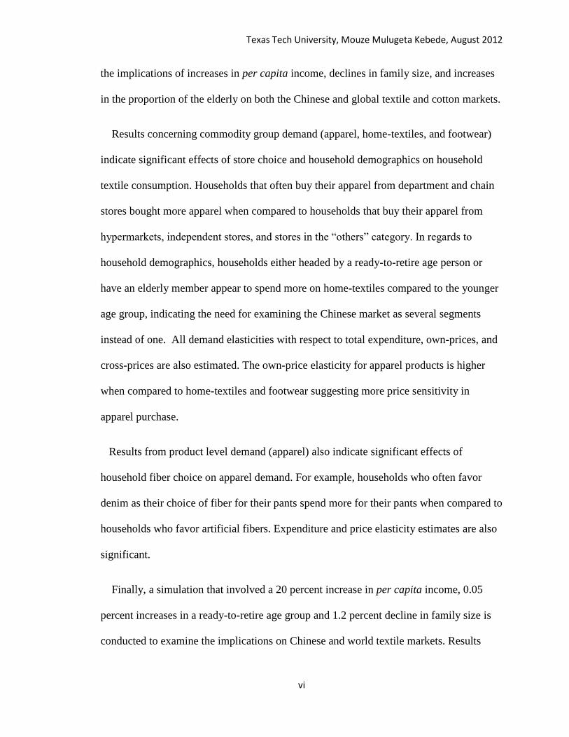
the implications of increases in per capita income, declines in family size, and increases
in the proportion of the elderly on both the Chinese and global textile and cotton markets.
Results concerning commodity group demand (apparel, home-textiles, and footwear)
indicate significant effects of store choice and household demographics on household
textile consumption. Households that often buy their apparel from department and chain
stores bought more apparel when compared to households that buy their apparel from
hypermarkets, independent stores, and stores in the “others” category. In regards to
household demographics, households either headed by a ready-to-retire age person or
have an elderly member appear to spend more on home-textiles compared to the younger
age group, indicating the need for examining the Chinese market as several segments
instead of one. All demand elasticities with respect to total expenditure, own-prices, and
cross-prices are also estimated. The own-price elasticity for apparel products is higher
when compared to home-textiles and footwear suggesting more price sensitivity in
apparel purchase.
Results from product level demand (apparel) also indicate significant effects of
household fiber choice on apparel demand. For example, households who often favor
denim as their choice of fiber for their pants spend more for their pants when compared to
households who favor artificial fibers. Expenditure and price elasticity estimates are also
significant.
Finally, a simulation that involved a 20 percent increase in per capita income, 0.05
percent increases in a ready-to-retire age group and 1.2 percent decline in family size is
conducted to examine the implications on Chinese and world textile markets. Results

Texas Tech University, Mouze Mulugeta Kebede, August 2012
vii
suggest that such changes are likely to increase the domestic textile price index and
textile consumption. In regards to the global market, the changes in Chinese socio-
economic variables considered is expected to affect positively the A-index, world cotton
production, and world mill use.
Texas Tech University, Mouze Mulugeta Kebede, August 2012
viii
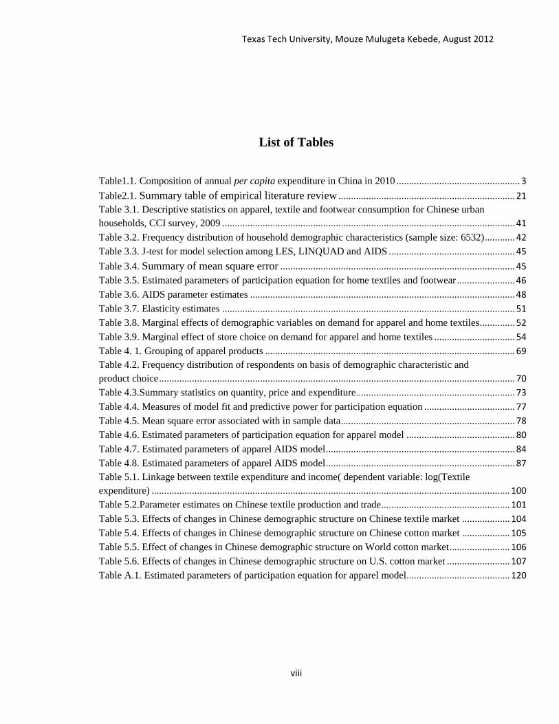
List of Tables
Table1.1. Composition of annual per capita expenditure in China in 2010 ................................................. 3
Table2.1. Summary table of empirical literature review ...................................................................... 21
Table 3.1. Descriptive statistics on apparel, textile and footwear consumption for Chinese urban
households, CCI survey, 2009 .................................................................................................................... 41
Table 3.2. Frequency distribution of household demographic characteristics (sample size: 6532) ............ 42
Table 3.3. J-test for model selection among LES, LINQUAD and AIDS .................................................. 45
Table 3.4. Summary of mean square error ............................................................................................. 45
Table 3.5. Estimated parameters of participation equation for home textiles and footwear ....................... 46
Table 3.6. AIDS parameter estimates ......................................................................................................... 48
Table 3.7. Elasticity estimates .................................................................................................................... 51
Table 3.8. Marginal effects of demographic variables on demand for apparel and home textiles .............. 52
Table 3.9. Marginal effect of store choice on demand for apparel and home textiles ................................ 54
Table 4. 1. Grouping of apparel products ................................................................................................... 69
Table 4.2. Frequency distribution of respondents on basis of demographic characteristic and
product choice ............................................................................................................................................. 70
Table 4.3.Summary statistics on quantity, price and expenditure ............................................................... 73
Table 4.4. Measures of model fit and predictive power for participation equation .................................... 77
Table 4.5. Mean square error associated with in sample data ..................................................................... 78
Table 4.6. Estimated parameters of participation equation for apparel model ........................................... 80
Table 4.7. Estimated parameters of apparel AIDS model ........................................................................... 84
Table 4.8. Estimated parameters of apparel AIDS model ........................................................................... 87
Table 5.1. Linkage between textile expenditure and income( dependent variable: log(Textile
expenditure) .............................................................................................................................................. 100
Table 5.2.Parameter estimates on Chinese textile production and trade ................................................... 101
Table 5.3. Effects of changes in Chinese demographic structure on Chinese textile market ................... 104
Table 5.4. Effects of changes in Chinese demographic structure on Chinese cotton market ................... 105
Table 5.5. Effect of changes in Chinese demographic structure on World cotton market ........................ 106
Table 5.6. Effects of changes in Chinese demographic structure on U.S. cotton market ......................... 107
Table A.1. Estimated parameters of participation equation for apparel model......................................... 120

Texas Tech University, Mouze Mulugeta Kebede, August 2012
ix
List of Figures
Figure 1.1. Per capita income and textile consumption in china 2000-08 ................................................... 5
Figure1.2.China population and its composition, 1978-2009 ....................................................................... 6
Figure1.3. Sales of apparel by major retail types, 2005-10 .......................................................................... 7
Figure3.1. Utility tree for household consumption in China ...................................................................... 32
Figure 4.1. Utility tree for household apparel consumption in China ......................................................... 61
Figure 4.2. Normal and KS estimate of density function for coats (hn=0.281) .......................................... 75
Figure 4.3. Normal and KS estimate of density function for pants (hn=0.281) .......................................... 76
Figure 5.1. China vs. World per-capita fiber consumption ......................................................................... 91
Figure 5.2.Effects of Chinese demographic and economic changes on World textile and cotton
market ......................................................................................................................................................... 95
Figure B.1.Probability density function for error terms of coats market participation
equation ................................................................................................................................................... 123
Figure B.2. Probability density function for error terms of pants market participation equation ............. 124
Texas Tech University, Mouze Mulugeta Kebede, August 2012
1
Chapter One
Introduction
Recent studies underscore the importance of investigating the potential of newly
industrialized economies (NICs)1 as markets for textiles given an increase in their
domestic per capita income (Dickens). A good case for these studies could be the
Chinese textile market where economic growth, coupled with changes in population
structure, has changed the composition of textiles consumed. Various indicators have
shown a change in the structure of textile consumption in China; for example, consumers
have developed a strong preference for imported apparel over time (Zhang et al.;
Abernathy et al.). In addition, household consumption has grown by approximately 7.5%
over the last decade and is even expected to overtake Japan’s household consumption, by
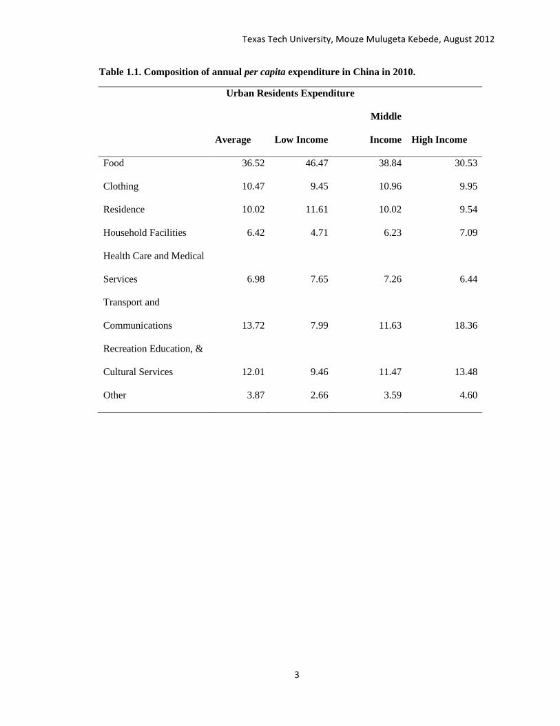
some estimates, in the next decade (Hansakul). A close look at household consumption
in urban and rural areas of China indicates that clothing expenditures are one of the most
important expenses amongst Chinese households (Table1) and constitute a higher share
of the household income when compared to similar figures for the U.S ($3.5 of $100
spent by a given household in 2009 in the U.S). China is also the world’s second largest
consumer market for cotton products and is slowly closing the gap with respect to the
U.S. in market size (PCI Fibers).
1 UNIDO (2009) defines NICs as major exporters of manufacturing among developing countries
in the mid 1970s and 1980’s, with a share of manufactures in total merchandise exports exceeding
20%. These economies include, in Asia: the Chinese Economic Area (China, Hong Kong and
Taiwan), South Korea, Singapore, Indonesia, Malaysia and Thailand and India. In Latin
America: Mexico, Brazil and Argentina.
Texas Tech University, Mouze Mulugeta Kebede, August 2012
2
Despite the increasing evidence that signal the importance of China as a consumer in
global textile and cotton markets, information and research about consumers in China has
been extremely limited. Given China’s status as one of the world’s largest markets for
cotton products (Pan et al., 2005), which underscores its relative importance as a major
player in global cotton markets, trends in Chinese demographics and associated changes
in domestic consumption patterns are likely to have impacts beyond the textile industry.
The growing importance of this poorly understood component of China’s cotton demand
suggests that an empirically based analysis of China’s household consumption would
bear important insights into the future evolution of world textile demand, exports and
prices.
Texas Tech University, Mouze Mulugeta Kebede, August 2012
3
Table 1.1. Composition of annual per capita expenditure in China in 2010.
Urban Residents Expenditure
Average Low Income
Middle
Income High Income
Food 36.52 46.47 38.84 30.53
Clothing 10.47 9.45 10.96 9.95
Residence 10.02 11.61 10.02 9.54
Household Facilities 6.42 4.71 6.23 7.09
Health Care and Medical
Services 6.98 7.65 7.26 6.44
Transport and
Communications 13.72 7.99 11.63 18.36
Recreation Education, &
Cultural Services 12.01 9.46 11.47 13.48
Other 3.87 2.66 3.59 4.60
Texas Tech University, Mouze Mulugeta Kebede, August 2012
4
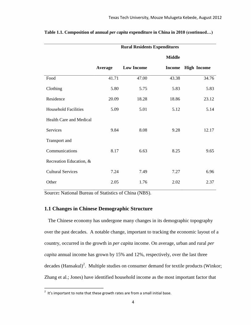
Table 1.1. Composition of annual per capita expenditure in China in 2010 (continued…)
Rural Residents Expenditures
Average Low Income
Middle
Income High Income
Food 41.71 47.00 43.38 34.76
Clothing 5.80 5.75 5.83 5.83
Residence 20.09 18.28 18.86 23.12
Household Facilities 5.09 5.01 5.12 5.14
Health Care and Medical
Services 9.84 8.08 9.28 12.17
Transport and
Communications 8.17 6.63 8.25 9.65
Recreation Education, &
Cultural Services 7.24 7.49 7.27 6.96
Other 2.05 1.76 2.02 2.37
Source: National Bureau of Statistics of China (NBS).
1.1 Changes in Chinese Demographic Structure
The Chinese economy has undergone many changes in its demographic topography
over the past decades. A notable change, important to tracking the economic layout of a
country, occurred in the growth in per capita income. On average, urban and rural per
capita annual income has grown by 15% and 12%, respectively, over the last three
decades (Hansakul)2. Multiple studies on consumer demand for textile products (Winkor;
Zhang et al.; Jones) have identified household income as the most important factor that
2 It’s important to note that these growth rates are from a small initial base.
Texas Tech University, Mouze Mulugeta Kebede, August 2012
5
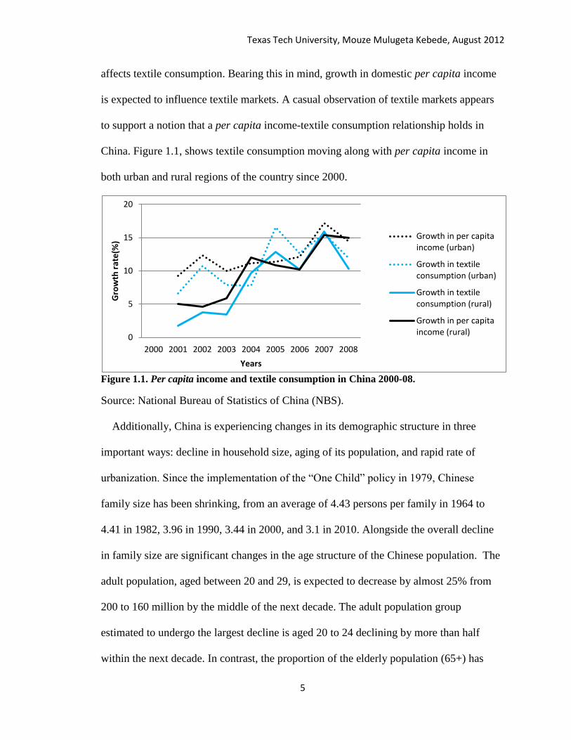
affects textile consumption. Bearing this in mind, growth in domestic per capita income
is expected to influence textile markets. A casual observation of textile markets appears
to support a notion that a per capita income-textile consumption relationship holds in
China. Figure 1.1, shows textile consumption moving along with per capita income in
both urban and rural regions of the country since 2000.
Figure 1.1. Per capita income and textile consumption in China 2000-08.
Source: National Bureau of Statistics of China (NBS).
Additionally, China is experiencing changes in its demographic structure in three
important ways: decline in household size, aging of its population, and rapid rate of
urbanization. Since the implementation of the “One Child” policy in 1979, Chinese
family size has been shrinking, from an average of 4.43 persons per family in 1964 to
4.41 in 1982, 3.96 in 1990, 3.44 in 2000, and 3.1 in 2010. Alongside the overall decline
in family size are significant changes in the age structure of the Chinese population. The
adult population, aged between 20 and 29, is expected to decrease by almost 25% from
200 to 160 million by the middle of the next decade. The adult population group
estimated to undergo the largest decline is aged 20 to 24 declining by more than half
within the next decade. In contrast, the proportion of the elderly population (65+) has
0
5
10
15
20
2000 2001 2002 2003 2004 2005 2006 2007 2008
Gro
wth
rat
e(%
)
Years
Growth in per capita income (urban)
Growth in textile consumption (urban)
Growth in textile consumption (rural)
Growth in per capita income (rural)

Texas Tech University, Mouze Mulugeta Kebede, August 2012
6
increased over the years from an average of 3.56% in 1964 to 4.9% in 1982, 6.2% in
1995, 7% in 2000, and 8.5% in 2009. Moreover, due to the dramatic fertility declines
over the last 30 years, the median age of the population is expected to increase from 30
years in 2000 to 47 in the next four decades (Wang). One effect of such a rapid increase
in size of the elderly population will be on domestic demand for textiles as the young
population is identified as the most active consumers of textiles in the literature (Wagner;
Lee et al.; Wagner and Mokhtari). A rapid rate of urbanization is also another feature of
the Chinese economy as depicted in Figure 1.2. The figure shows the urban population
growing, on average, by 3.9 percent, which is larger than the national average of 0.8
percent, while rural population has been declining both in proportion and size since 1978.
Results regarding the impact of geographic location and family size on textile demand,
however, are inconclusive in the literature with some reporting significant while others
indicating negligible effects.
Figure 1.2. China population and its composition, 1978-2009.
Source: National Bureau of Statistics of China (NBS).
1.2 Changes in Shopping Habits of Chinese Households
Traditionally, the role of retailers is often limited to a link between manufacturer and final
consumers. Yet, with continuous change in consumer taste for products, the role retailers play has
0.00
20.00
40.00
60.00
80.00
100.00
19
78
19
80
19
85
19
90
19
91
19
92
19
93
19
94
19
95
19
96
19
97
19
98
19
99
20
00
20
01
20
02
20
03
20
04
20
05
20
06
20
07
20
08
Rat
io
Years
urban
rural

Texas Tech University, Mouze Mulugeta Kebede, August 2012
7
increased beyond that of intermediary over the years. In doing so, a variety of marketing
strategies are used by these retailers that ranges from expert knowledge on the product they sell
in the case of specialty stores to one-stop shopping experience for consumers in the case of
hypermarkets and department stores. Such strategies are implemented with the main objective of
increasing sales of retail store products, but little is known whether store strategies such as in-
store service, store design, and ambiance translate to increased sales of apparel and textiles.
China, with joining of WTO in 2001, has opened its retail sector to more foreign investment.
This, in turn, has resulted in a rapid increase in the numbers of western-style retail outlets (Kim
and Kincade). Many of the new retailers offer both domestic and foreign brands, and Chinese
consumers’ view shopping at these retail outlets and dressing foreign brands as superior as the
price they command is relatively higher. As shown in Figure 1.3, with an increase in the living
standard of Chinese citizens, specialty and department stores have increased their market share
for apparel products constituting over 60 percent of sales revenue in 2010 (Li and Fung Research
Centre). Another point worth noting from the figure below is that hyper and wholesale markets
have seen their share declining or unchanged over recent years.
Figure 1.3. Sales of apparel by major retail types: 2005-10.
Source: Li and Fung Research Centre (2011).
0
5
10
15
20
25
30
35
40
2004 2005 2006 2007 2008 2009 2010 2011
% R
eta
il sa
les
Years
Hyper markets
Department stores
Speciality stores
Other non grocery retailing (e.g:factory outlets, free markets) Non store retailing(e.g: internet)
Texas Tech University, Mouze Mulugeta Kebede, August 2012
8
1.3 Specific Problem
Given the relatively higher budget share of clothing of Chinese households ($5.8 for every $100)
compared to the developed world such as the U.S ($3.5 for every $100) and the rapid increase in
Chinese household income observed in recent years, domestic demand for apparel is expected to
grow rapidly. According to the National Bureau of statistics (NBS), per capita apparel
expenditure of urban households has increased on average by 12.5% to 1444.34 Yuan in 2010,
while cash expenditure on apparel of the lowest income rural households rose to 150.84 Yuan, up
by 11.9% from its 2009 value. Such a rapid growth rate, according to some analysts, is expected
to make China one of the largest markets for apparel by 2020 outpacing Japanese consumption by
over 120% (Kurt Salmon Associates as cited in Zhang et al.). Moreover, the structure of
consumption has changed significantly over recent years: sales in the high-end apparel
segments have increased by over 30 percent, higher than the growth rate in the low-end
segment (18.4%) and the national average (21.2%) in 2010 (Li and Fung Research Centre,
2011). On the other side of the picture, however, China is also experiencing a dramatic
decline in family size and an increase in the percentage of old population. Such changes
in population structure, according to previous literature, are likely to have an inverse
impact on the consumption pattern of textiles.
Despite such considerable changes in the Chinese apparel market, research concerning
Chinese household demand for textiles is currently limited. To better meet consumer
demand and understand the implications of these changes on global markets, however, it
is critical to understand the factors that shape consumer preferences in China.

Texas Tech University, Mouze Mulugeta Kebede, August 2012
9
1.5 Objectives of the Study
The general purpose of this study is to examine the effects of China’s economic growth
and the changes in China’s demographic composition on its textile, apparel, and cotton
markets. Specifically, this study:
examines the impact of the socio-economic changes, product quality attributes,
and shopping habits on the aggregated and disaggregated textile product mix, and
analyzes the effect of the changes in Chinese textile consumption pattern on
global cotton markets.
Texas Tech University, Mouze Mulugeta Kebede, August 2012
10
CHAPTER TWO
Review of Literature
The first section of this chapter provides a review of the various theoretical and empirical models
used in demand analysis. The advantages and limitations associated with each of the models are
also explained. The second section reviews research studies that have used the Global Fiber
Model (GFM) developed by the Cotton Economic Research Institute at Texas Tech
University. The GFM is also be used in this study to explain the implications of Chinese
socio-economic changes on the global cotton market.
2.1 Review of Demand Functional Forms
This section surveys four major complete demand functional forms and one incomplete
demand system: the Linear Expenditure System (LES), Rotterdam model, Translog
Demand System, Almost Ideal Demand System (AIDS), and LINQUAD demand system,
respectively. Using the pure theory of consumer behavior as a starting point, where
consumer choice of quantity consumption is subject to a budget constraint, the earliest
approach in demand analysis used was a logarithmic functional form.
Denoting q1…. qn as quantities consumed of n goods and p1….pn as the corresponding
prices, and total expenditure as the summation of expenditure on each commodity
purchased, the demand for a good is specified as:
2.1
where is the intercept; is product i income elasticity; and is the cross price
elasticity of jth
price on ith
demand. To reduce the number of variables for estimation,

Texas Tech University, Mouze Mulugeta Kebede, August 2012
11
Stone used the Slutsky equation for decomposing the cross-price elasticities. That is, the
double log equation can further be rewritten by decomposing the uncompensated cross
price elasticity using the Slutsky equation, , where
is the
compensated price elasticity and
is the budget share of good j . This derivation
has the following result:
2.2
Here, however, can be used as a general price index; based on this
specification, the demand function can be expressed in terms of real income and
compensated prices:
2.3
In estimating this model, the homogeneity restriction3 can be imposed as shown in
equation 2.4, but the adding up restrictions would not hold unless all income elastcities
are set to one. This limitation, in turn, has limited the use of this model for empirical
analysis.
2.4
In 1954, Stone was able to use the first system of demand equations that was consistent
with theoretical restrictions of demand analysis. According to the LES, proposed by
3 Homogeneity restriction relates to the fact that for any good, the sum of its own-price
elasticity, all of the related cross-price elastcities and its income elasticity should be zero.
i.e: no money illusion.
Texas Tech University, Mouze Mulugeta Kebede, August 2012
12
Klein and Rubin, expenditure on a given commodity can be specified as a linear function
of n prices and income:
2.5
where is the coefficient for the price of the specific good analyzed. The
first component of this equation is referred to as “subsistence consumption”, while the
second term on the right-hand side of the above equation is referred to as “supernumerary
income.” The LES is derived from Stone-Geary utility function:
For his analysis, Stone used British consumers’ purchased goods data over the years
1920-38 and applied the theoretical restrictions of adding up, homogeneity, and
symmetry to limit the number of parameters to be estimated. These theoretical
restrictions gave the LES an attractive feature for use in demand analysis; yet, empirical
investigations of the model revealed some limitations for use in practice. A primary
limitation is that the model does not allow net complementary4 interaction among goods.
The Rotterdam model, proposed by Thiel and Barten, is an extension to the double
logarithmic model. This model uses differentials in contrast to level logarithmic forms
used in Stone’s model. This modification has enabled researchers to overcome many of
the limitations in the double logarithmic form, especially in estimating the substitution
matrix and determining substitutes and complements from direct estimation.
4 Two goods, xi and xj, are referred as net complements if

Texas Tech University, Mouze Mulugeta Kebede, August 2012
13
Derivation of the model starts by totally differentiating equation 2.1, which has the
following result:
2.6
After incorporating the Slutsky decomposition, as in equation 2.2, and multiplying the
result with the budget share wi to impose symmetry, the final equation becomes:
2.7
The testable restrictions of this model are: Empirical
investigation of this model initially carried out by Barten and then Deaton, however,
showed that the Rotterdam model failed in satisfying the homogeneity restriction, which
triggered the search for a more theoretically consistent demand system.
Unlike the previous two demand models, the indirect Translog demand system of
Christensen, Jorgenson, and Lau uses duality theory and builds its analysis on an indirect
utility or a cost function. It specifies the log of an indirect utility function as a function of
the log of prices to expenditure ratios as shown in equation 2.8. The function satisfies
homogeneity in prices without directly imposing the restriction.
2.8
Using Roy’s identity, the Marshallian demand functions can be specified as shown in
Equation 2.9. Despite its flexible functional form, Clements and Selvanathan indicate
that the model has limited use in empirical work as parameter estimates are difficult to
interpret because of the complex form of the variables.
Texas Tech University, Mouze Mulugeta Kebede, August 2012
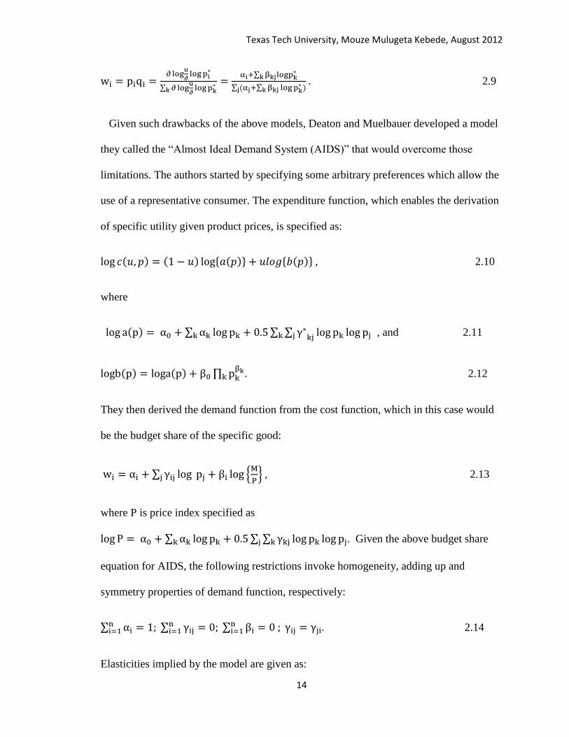
14
2.9
Given such drawbacks of the above models, Deaton and Muelbauer developed a model
they called the “Almost Ideal Demand System (AIDS)” that would overcome those
limitations. The authors started by specifying some arbitrary preferences which allow the
use of a representative consumer. The expenditure function, which enables the derivation
of specific utility given product prices, is specified as:
2.10
where
, and 2.11
2.12
They then derived the demand function from the cost function, which in this case would
be the budget share of the specific good:
2.13
where P is price index specified as
. Given the above budget share
equation for AIDS, the following restrictions invoke homogeneity, adding up and
symmetry properties of demand function, respectively:
2.14
Elasticities implied by the model are given as:
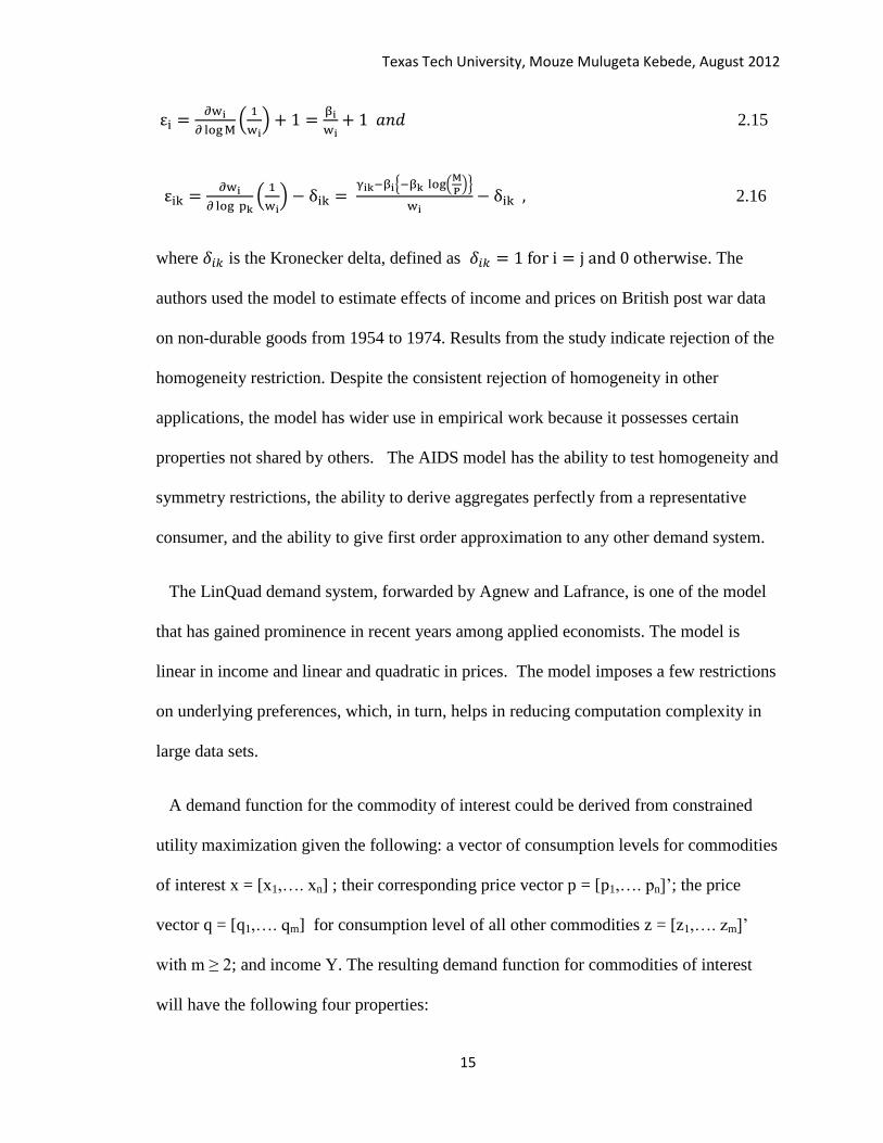
Texas Tech University, Mouze Mulugeta Kebede, August 2012
15
2.15
2.16
where is the Kronecker delta, defined as . The
authors used the model to estimate effects of income and prices on British post war data
on non-durable goods from 1954 to 1974. Results from the study indicate rejection of the
homogeneity restriction. Despite the consistent rejection of homogeneity in other
applications, the model has wider use in empirical work because it possesses certain
properties not shared by others. The AIDS model has the ability to test homogeneity and
symmetry restrictions, the ability to derive aggregates perfectly from a representative
consumer, and the ability to give first order approximation to any other demand system.
The LinQuad demand system, forwarded by Agnew and Lafrance, is one of the model
that has gained prominence in recent years among applied economists. The model is
linear in income and linear and quadratic in prices. The model imposes a few restrictions
on underlying preferences, which, in turn, helps in reducing computation complexity in
large data sets.
A demand function for the commodity of interest could be derived from constrained
utility maximization given the following: a vector of consumption levels for commodities
of interest x = [x1,…. xn] ; their corresponding price vector p = [p1,…. pn]’; the price
vector q = [q1,…. qm] for consumption level of all other commodities z = [z1,…. zm]’
with m ≥ 2; and income Y. The resulting demand function for commodities of interest
will have the following four properties:

Texas Tech University, Mouze Mulugeta Kebede, August 2012
16
(i) The demands are positive valued, hx (p,q,y)≥0
(ii) The demands are zero degree homogeneous in all prices and income,
hx (p,q,y)= h
x (tp,tq,ty) fr all t≥0
(iii) The n x n matrix of compensated substitution effects for x, ∂hx/∂p’+∂h
x/∂y h
x’
is symmetric, negative semidefinite, and
(iv) Income is greater than total expenditure on a proper subset of the goods
consumed, p’hx(p,q,y)<y
The first three properties are identical for both complete and incomplete demand
systems, while the last property is a feature of an incomplete demand system that
distinguishes it from complete demand systems. However, such a difference could be
removed with the use of a composite good for goods not being included in the analysis.
Expenditure on the composite good is expressed as S=q’z=y-p’x. The four properties
identified above and the budget identity will, in turn, give a quasi-expenditure function
that is increasing and concave in p, and linearly homogeneous in p and q. The quasi-
expenditure function is related to expenditure function using the following identity:
2.17
2.18
2.19
where p is the vector of prices, is an arbitrary real value function for all variables in
q, is the constant of integration, and are vectors of parameters to be
estimated. Using Shepherd’s Lemma, the demand function can be specified as:

Texas Tech University, Mouze Mulugeta Kebede, August 2012
17
2.20
And the corresponding expenditure function could be obtained by multiplying both sides
of 2.20 by commodity corresponding prices:
2.21
The advantage of this demand specification is that it is theoretically consistent and can
directly provide an exact measure of welfare. Homogeneity is imposed by using real
prices and income, symmetry is imposed in the B matrix with each element Bij=Bji; and
adding-up is always satisfied as a property of an incomplete demand system.
The standard Marshallian income and price elasticity formula for the LinQuad are;
2.22
In contrast to the complete demand models discussed above that focused only on
income and price effects, demand analysis also needs to incorporate household and
product characteristics that are likely to generate differences in consumption patterns
across household and products with different characteristics. Pollak and Wales describe
Barten as the first to pioneer the use of demographic incorporated demand systems
consistent with economic theory. Pollak and Wales identify two ways of adding this
information into complete demand systems: the first uses un-pooled data while the
second makes use of pooled data. The first method involves separating households into
different sub samples on the basis of demographic profiles and using the above demand
models for each sample separately. This approach results in different parameter estimates
Texas Tech University, Mouze Mulugeta Kebede, August 2012
18
for households with different demographic variables. Accordingly, the effect of each
demographic variable on consumption decisions could be inferred without even having
the demographic variables included in the demand model.
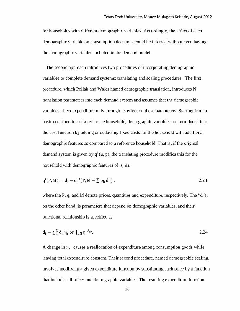
The second approach introduces two procedures of incorporating demographic
variables to complete demand systems: translating and scaling procedures. The first
procedure, which Pollak and Wales named demographic translation, introduces N
translation parameters into each demand system and assumes that the demographic
variables affect expenditure only through its effect on these parameters. Starting from a
basic cost function of a reference household, demographic variables are introduced into
the cost function by adding or deducting fixed costs for the household with additional
demographic features as compared to a reference household. That is, if the original
demand system is given by qi (u, p), the translating procedure modifies this for the
household with demographic features of as:
2.23
where the P, q, and M denote prices, quantities and expenditure, respectively. The “d”s,
on the other hand, is parameters that depend on demographic variables, and their
functional relationship is specified as:
2.24
A change in causes a reallocation of expenditure among consumption goods while
leaving total expenditure constant. Their second procedure, named demographic scaling,
involves modifying a given expenditure function by substituting each price by a function
that includes all prices and demographic variables. The resulting expenditure function

Texas Tech University, Mouze Mulugeta Kebede, August 2012
19
depends on all prices and demographic variables. Pollak and Wales’ empirical
investigation included the number of children and ages as demographic variables, and
used 1966 and 1972 data from the British Family Expenditure Survey series for analyzing
consumption decisions on food, clothing, and miscellaneous categories. Results from
their study strongly supported the inclusion of these variables. Food and clothing budget
shares increased with family size, while the miscellaneous share decreased implying
reallocation of expenditure. Child’s age was also found significant in the model,
affecting directly the budget share for food and clothing and inversely affecting for
miscellaneous. The scaling procedure resulted in a higher likelihood function value as
compared to the translating procedure for both quadratic and translog models.
Given the limitation of each of the demand models discussed above, this study nests two
of the complete demand systems (the LES and AIDS) with the LINQUAD model and
tests using a statistical procedure to identify the model that best fits in the household data
used in this study.
2.2 Review of Empirical Literature on Textile Demand
Demand for textile products has traditionally been investigated by using either per
capita textile consumption or the textile budget share as a dependent variable. The
selection of factors influencing consumption, on other hand, has largely been based on
economic theory or previous research findings. Research on textile expenditure has
identified household income as one of the most important determinants affecting textile
consumption. Results from these studies have found income elasticities ranging between
0.41 and 2.5, depending on the textile products considered and the demographic group
analyzed as shown in Table 2.1.

Texas Tech University, Mouze Mulugeta Kebede, August 2012
20
Table 2.1. Summary table of empirical literature review.
Results Model used Data used Author
Income elasticity range : 0.5-2
Price elasticity range : 0.37-1.1
Single equation model
on clothing
U.K 1987-
2000 , time
series
Jones and
Hayes (2002)
Income elasticity : 0.48-0.5
Price elasticity : 1-1.9
Single equation on
clothing expenditure
U.S 1929-
1987
Mokhtari
(1992)
Expenditure elasticity: 1.01 for girls -2.01 for fathers
Lower expenditure for older children than younger ones
Mothers education increases expenditure on herself and father
No significant effect of fathers education
No significant effect of mothers or fathers age on their own expenditure
Young mothers with increased expenditure on girls and older mothers on
boys
Young fathers with increased expenditure on mothers and boys and older
fathers with decrease expenditure on boys
Single equation on
clothing ( double log)
CES1986 Nelson (1989)
Income elasticity: 0.4-0.62
Women headed household spend more on apparel than male headed
households
Household heads with more education have higher expense on apparel
than those with less education
Negative or no significant effect of household size
Single equation on
clothing ( double log)
CES 1990 Wagner and
Mokhtari
(2000)
Income elasticity: 0.72-0.80
Positive effect of family size
Negative effect of household head age
Single equation on
home textiles
CES1973 Wagner (1986)
Texas Tech University, Mouze Mulugeta Kebede, August 2012
21
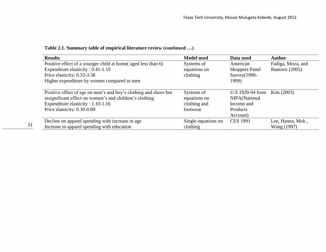
Table 2.1. Summary table of empirical literature review (continued …)
Results Model used Data used Author
Positive effect of a younger child at home( aged less than 6)
Expenditure elasticity : 0.41-1.19
Price elasticity: 0.33-3.38
Higher expenditure by women compared to men
Systems of
equations on
clothing
American
Shoppers Panel
Survey(1990-
1999)
Fadiga, Misra, and
Ramirez (2005)
Positive effect of age on men’s and boy’s clothing and shoes but
insignificant effect on women’s and children’s clothing
Expenditure elasticity : 1.10-1.16
Price elasticity: 0.39-0.89
Systems of
equations on
clothing and
footwear
U.S 1929-94 from
NIPA(National
Income and
Products
Account)
Kim (2003)
Decline on apparel spending with increase in age
Increase in apparel spending with education
Single equations on
clothing
CES 1991 Lee, Hanna, Mok ,
Wang (1997)
Texas Tech University, Mouze Mulugeta Kebede, August 2012
22
Winakor, using survey data from three states (Nebraska, Iowa, and Illinois), found that
expenditure elasticities were inelastic for household textiles. Supporting results were also
reported by Wagner from his analysis of consumer expenditure survey data from 1973.
Results in regards to apparel products, on other hand, indicated mixed findings. Nelson,
using U.S. expenditure survey data from 1985, found higher expenditure elasticities for
apparel products with the fathers’ apparel having the highest elasticity when compared to
the children’s and mothers’ apparel. Higher apparel expenditure elasticities were also
reported from time series studies on U.K. consumers by Jones and Hayes and on U.S.
consumers by Kim. Fadiga, Misra, and Ramirez, on other hand, found lower expenditure
elasticities for some apparel products when analyzing the products individually rather
than as a group.
Other important demographic variables identified in the literature include age of the
household members, family size, family composition, geographic location, and the
gender, education, and occupation of the household head. Elderly consumers were
reported to spend less money in general for both home textiles and apparel (Wagner; Lee
et al.; Wagner and Mokhtari). Lee et al. focused on the influence of age, especially of the
elderly, on the demand for apparel. Using a nonlinear demand system and a life cycle
approach5 to consumption, they found declining expenditure levels for apparel after the
age of 68, which they attributed largely to increase expense for health and other age
related services. Similar results were also reported by Wagner and Mokhtari in their
analysis of quarterly U.S. household apparel expenditure. The effect of marital status on
textile expenditure is difficult to ascertain from the literature as some reported a
5 The life cycle hypothesis states that consumption decisions of households depend not
only on current income, but also on future anticipated circumstances.
Texas Tech University, Mouze Mulugeta Kebede, August 2012
23
significant and positive effect on textile expenditure (Wagner; Lee et al.) while others
reported no statistically significant effect (Wagner and Mokhtari).
The effect of family size on textile consumption was inconclusive in the literature with
some reporting a positive correlation (Winakor; Wagner), while others an inverse effect
(Wagner and Mokharti). Though the larger a family the more the textile requirements, the
effect might be minimized owing to the fact that economies of scale may be operative in
a large family as reported in Wagner and Mokharti. Winakor found that expenditure on
household textiles increased by $3.40 for each additional family member, while Wagner
and Mokharti reported an inverse relationship between apparel expense and family size
during the winter season and no statistically significant relationship for other seasons.
The effect of family composition indicated higher textile expenditure for both apparel
and home textiles for each female member in a household when compared to a male
counterpart. Winakor reported that expenditures for household textiles increased by a
different amount for each additional adult woman in a family: by $35 for farm families
and $45 for city families. Supporting results for apparel expenditure were also reported
by Nelson in his analysis of individual clothing consumption within a household.
Clothing expenditures on boys constituted only 81% of the spending on girls, while
expenditure on fathers’ clothing constituted only 62% of expenditures on mothers’.
Wagner also reported a significant effect of age of the youngest child on home textiles,
with families having children under six spending more on home textiles than families
with no children below six. In regards to gender, female headed households, in general,
spent more on apparel expenditures than did male headed households (Wagner and
Mokharti; Lee et al.; Fadiga, Misra and Ramirez).
Texas Tech University, Mouze Mulugeta Kebede, August 2012
24
On another dimension, evaluation of the effects of product attributes indicates that a
product’s price as the most important determinant in textile consumption. Fadiga, Misra,
and Ramirez reported demand for apparel products is own-price elastic. Cross-price
elasticities among apparel products reported were less than one and negative implying
complements. Supporting results were also reported by Mokhatri from his time series
analysis of U.S clothing expenditure and by Jones and Hayes from their time series
analysis of U.K clothing consumption. Other product attributes identified important in the
literature include fiber content (Fadiga, Misra, and Ramirez) and product origin (Zhang et
al.). Fadiga, Misra, and Ramirez reported higher expenditure shares for most apparel
products, with exception of male slacks, with 100 percent cotton than products with less
than 50 percent cotton blend. Zhang et al found country of origin as an important
attribute in the consumer’s purchasing decision.
Much of the economic studies discussed above were conducted for households living in
the developed world and there exist limited information on households’ textile
consumption behavior regarding the developing world. This study helps in bridging this
gap as it mainly focuses on Chinese households’ textile consumption patterns, one of the
largest and most rapidly developing part of the world. In addition, most of the studies
reviewed above, with exception to Kim; and Fadiga, Misra, and Ramirez work, are not
presented in a system of demand equations framework. This study attempts to address
those limitations and develops household demand models for textile products using a
framework consistent with economic theory. In addition, this study analyzes the demand
for textiles at a disaggregate level, thus identifing potential relationships between textile
products.

Texas Tech University, Mouze Mulugeta Kebede, August 2012
25
2.3. Review of the Global Fiber Model
The global fiber model was mainly developed to explain the impacts of global trade liberalization
on the competitiveness of U.S. cotton industry. To this effect, the model incorporates inter-fiber
competition between artificial and natural fibers in textile mill use, regional production
heterogeneity within major cotton producing countries and a linkage between upstream and raw
fiber sector for major cotton producing countries. The partial equilibrium model includes
production, demand, ending stocks and market clearing conditions for both cotton and artificial
fibers for 24 countries analyzed within the model.
Cotton production, Equation 2.25 through 2.27, is specified as a product of yield (YLDi) and
harvested area (ACRi). Cotton harvested area (ACRic) in the i
th region is specified as a
function of the ratio of expected net return of cotton (ENRic) to competing crops (ENRi
o)
and a time trend (T). Previous year’s net return is used as a proxy for expected return in
the current period. Assuming constant returns to scale in production, it is modeled as a
function of a lag of rainfall (LRFi), expected farm price ( ), and a time trend (T).
PRDic= YLDi
c * ACRi
c, 2.25
, and 2.26
2.27
The next step involves estimation of fiber demand models. The demand for all fibers
(DMfi) is specified as a function of a constant term for autonomous consumption (DMi),
the fiber price index (FPRi), and gross domestic product (GDPi):
2.28
Texas Tech University, Mouze Mulugeta Kebede, August 2012
26
In the second step, total fibers are divided into cotton, wool, and man-made fibers.
Demand for cotton ( ) is, thus, a product of aggregate fiber demand and a proportion
of cotton in total fiber use. A share equation for cotton (DSc) is modeled as a function of
the ratio of the domestic price for cotton (PDci) and the domestic man-made fiber price
(PDm
i):
2.29
2.30
For man-made fibers, the supply function (PDRim
) is modeled through the estimation of
production capacity (CPTi) and capacity utilization (CPUi). Man-made fibers production
capacity is modeled as a function of the lag of the man-made fiber domestic price
(LPDm
i), the lag of the oil price (LPDli) and a lag of capacity (LCPTi):
2.31
Total capacity utilization, on the other hand, is modeled as a function of a ratio of the
current domestic man-made fiber price (PDm
i) and current oil price (PDli) and a lag of
capacity utilization (LCPUm
i):
. 2.32
Multiplying production capacity by capacity utilization yields total man-made fiber
production:
2.33

Texas Tech University, Mouze Mulugeta Kebede, August 2012
27
Cotton export demand (XPDi) is modeled as a function of the ratio of international cotton
price (Pw) converted to domestic currency by applicable exchange rate (XRi) and
domestic cotton prices (PDci):
2.34
The import demand equation for cotton (IMDi) for cotton is expressed as a function of
international cotton price, exchange rates, tariff rates (ti), and quota restrictions:
2.35
Domestic market equilibrium is obtained by equalizing demand and supply side
equations: ending stocks plus domestic demand and exports equal beginning stocks plus
production and imports:
2.36
Solving this equilibrium yields the domestic price for cotton. The world price for cotton
(A-index), the cotton textile price index, and man-made fiber price are solved by
equalizing world imports ( to world exports ( ).
2.37
Much of the research studies based on this model focus on changes on the supply side policies.
Notable among these include the Pan et al. (2007) study that analyzed removal of domestic
subsidies and border tariffs for cotton in the international market; Fadiga et al. (2008) who
examined the impact of unilateral removal of the total U.S aggregate measure of support (AMS)
and a multilateral trade reform where U.S AMS payment reductions are matched by multilateral
tariff and subsidy elimination from the rest of the world; and Pan et al. (2006) who looked into

Texas Tech University, Mouze Mulugeta Kebede, August 2012
28
the effects of Chinese currency evaluation on the world fiber market. This study, on the other
hand, will use the global fiber model to analyze effects of changes in Chinese textile demand
structure on global fiber market.

Texas Tech University, Mouze Mulugeta Kebede, August 2012
29
Chapter Three
Choice of Retail Outlets and Chinese Household Demand for Textiles
and Footwear: Analysis Using Alternative Demand Functional Forms
Introduction
This study focuses on the potential impact of households shopping habits and socio-economic
profiles on the demand for textiles. Research regarding the impact of household shopping
behavior on demand for textiles is limited. Quantifying the impact is important for both retailers
looking for optimal marketing strategies and manufacturers considering choice of distribution
channel for their products. Besides the changes in the structure of retail outlets for textiles,
marked changes have occurred in the socioeconomic profile of Chinese population in
recent years. These changes are likely to have important implications not only for the
textile industry, but also for upstream production sectors. Given this fact, the study looks
in the effects of changes in the socioeconomic structure of Chinese population on demand
for textile products. The research, along the way, implements a statistical model that nests
three demand functional forms (LES, AIDS and LinQuad incomplete demand systems) to
choose the functional form that best fits the data.
The major objective of this study is to determine whether household choice of retail outlets has an
impact on Chinese demand for textiles. In particular, this study attempts to answer two
questions:
How Chinese aggregate demand for each category of textile (apparel, home
textile, and footwear) is affected by household choice of retail outlets, and
changes in prices?
Texas Tech University, Mouze Mulugeta Kebede, August 2012
30
How does the change in Chinese demographic structure (increased proportion of
elderly, family size) affect Chinese aggregate expenditure shares for apparel,
home textiles, and footwear?
3.1 Conceptual Framework
In constructing a demand model for commodities, a two-step budgeting structure is
used as illustrated by Deaton and Mullbauer (1980). Preferences are assumed weakly
separable across broad consumer goods, and weakly separable across time. As shown in
Figure 3.1, the consumer allocates his expenditure to broad group of products such as
food, clothing or housing in the first stage. And in second stage, expenditures allocated
for broad groups are reallocated again among elements of the broad group in such a way
that the preference structure within the sub-utility functions are determined independent
of goods belonging to other broad group. Given such a structure, the consumer’s utility
function can be specified as:
U [Q1, Q2… QN),] =U [u (q1), u (q2)… u (qN)] 3.1
Where U [.] is utility from the broad commodity groups while u (.) is a sub-utility
function within the broad group. Using Price (PB =YB/QB) and quantity (QB=u (q))
indices for a broad group as in Lewbel (1989), utility maximization for a broad group can
be written as:
Max U [u (q1), u (q2)… u (qN] s.t ∑ PB QB = YB 3.2
The solution to this problem gives us Marshallian demand for each broad group and the
corresponding expenditure associated for each broad commodity group. Given optimal

Texas Tech University, Mouze Mulugeta Kebede, August 2012
31
expenditure for each broad group, the consumer maximizes its sub-utility in the second
stage.
Max u (q) s.t ∑ pi qi= YB. 3.3
The solution to this problem gives us Marshallian demand for each element in the broad
commodity group. The advantage of such a structure is that it avoids the need to include
all commodities consumed by a household in estimating demand for a specific consumer
good or set of goods.
As the above framework puts no restriction on the sub-utility functions in analyzing
effects of socio-demographic factors, this process is used to develop the empirical
econometric procedure to recover elasticity estimates for textile consumption in China. A
diagrammatical explanation of the procedure is shown in Figure 3.1.
Household Consumption Expenditure
Textile and Footwear Expenditure Non- Textile & Footwear Expenditure
Apparel Footwear Home-Textiles
Figure 3.1. Utility tree for household consumption in China
Texas Tech University, Mouze Mulugeta Kebede, August 2012
32
3.2 Methods and Procedures
Demand systems (here after called systems) estimation most often addresses the
optimal allocation of goods and services and is concerned with how changes in income,
relative commodity prices, and tastes and preferences affect the consumers’ choice of
goods in a given period. Its history in applied work, according to Stigler as cited in
Clements and Selvanathan, can be traced back to Engle’s famous budget study of 1857.
Yet, it was almost after 100 years that Klein and Rubin developed a linear expenditure
system (LES) that was in line with the basic principles of consumer utility maximization.
Stone pioneered its empirical use, which has resulted in a breakthrough in the study of
demand analysis. His analysis was able to reduce the number of parameters to be
estimated and he was also able to test whether the resulting functional forms satisfy the
basic theoretical properties of demand functions. A number of models have also been
developed which include, the Rotterdam model (Thiel; Barten), the Translog model
(Christensen, Jorgensen and Lau), the Almost Ideal Demand System (Deaton and
Muellbauer), and the LinQuad incomplete demand system (Lafrance and Agnew).
These models were developed after the LES to circumvent problems associated with
previous models. Yet, the advantage that these models exhibit also prevents them in
certain ways from satisfying the theoretical conditions. For example, the great attraction
of the LES in empirical use relates to its linearity, simplicity and economy of
parameterization, which makes it easy to use and also satisfy regular conditions globally,
but fails from modeling behaviors having complex functional forms. On the other hand,
relatively complex demand functional forms are able to approximate fairly complicated
and flexible behaviors. But, their flexible and complex nature makes results from these
Texas Tech University, Mouze Mulugeta Kebede, August 2012
33
models difficult to interpret (Clements, Selvanathan) and sometimes these models are not
well behaved globally (Guilkey, Lovell and Sickles).
Given the above limitations, Alston and Chalfant discuss the importance of using a
statistically based model selection to explain consumption patterns of households.
Relying on the Alston and Chalfant argument, this study compares three common
demand specifications for analyzing Chinese household allocation of total textile
expenditures among broad categories of textile products and footwear. Three
approaches for comparison have been proposed in the literature. The encompassing
model, the J test, and the Cox test in choosing the better performing model on statistical
grounds (Greene). For the purpose of this analysis, the J-test approach initially proposed
by Davidson and Mackinnon is used because of its ease of implementation.
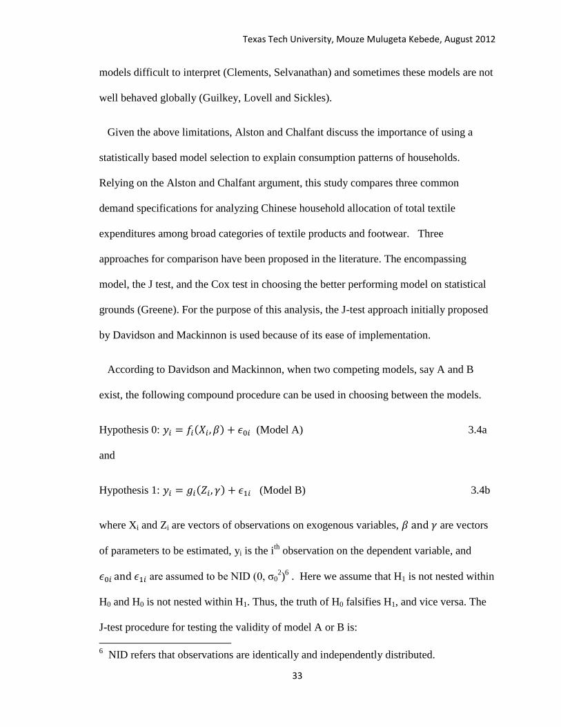
According to Davidson and Mackinnon, when two competing models, say A and B
exist, the following compound procedure can be used in choosing between the models.
Hypothesis 0: (Model A) 3.4a
and
Hypothesis 1: (Model B) 3.4b
where Xi and Zi are vectors of observations on exogenous variables, are vectors
of parameters to be estimated, yi is the ith
observation on the dependent variable, and
are assumed to be NID (0, σ02)6 . Here we assume that H1 is not nested within
H0 and H0 is not nested within H1. Thus, the truth of H0 falsifies H1, and vice versa. The
J-test procedure for testing the validity of model A or B is:
6 NID refers that observations are identically and independently distributed.
Texas Tech University, Mouze Mulugeta Kebede, August 2012
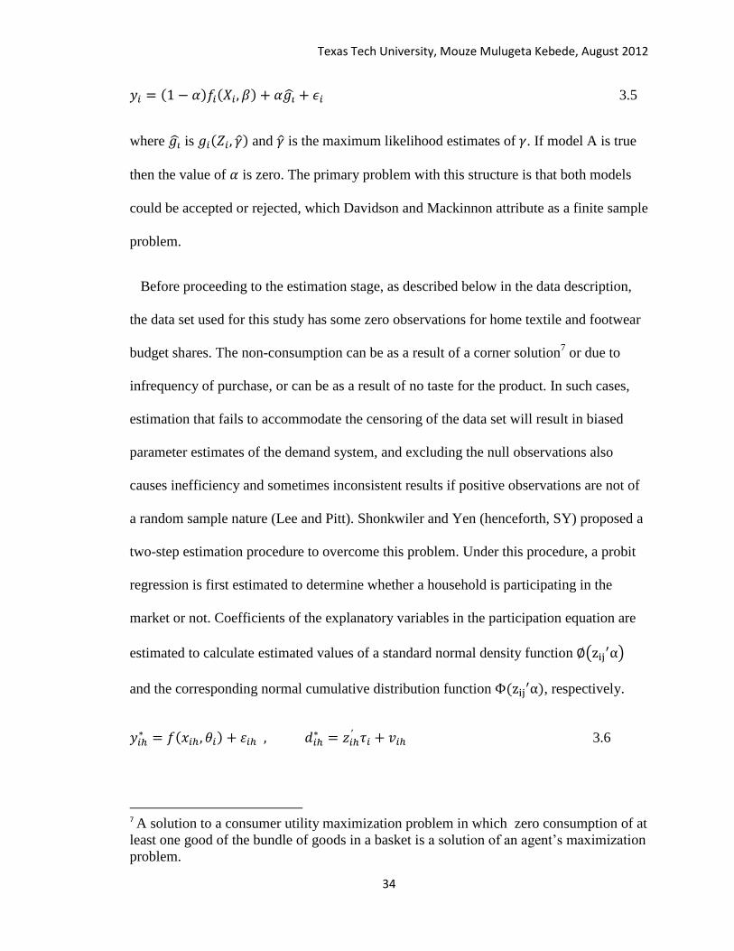
34
3.5
where is and is the maximum likelihood estimates of . If model A is true
then the value of is zero. The primary problem with this structure is that both models
could be accepted or rejected, which Davidson and Mackinnon attribute as a finite sample
problem.
Before proceeding to the estimation stage, as described below in the data description,
the data set used for this study has some zero observations for home textile and footwear
budget shares. The non-consumption can be as a result of a corner solution7 or due to
infrequency of purchase, or can be as a result of no taste for the product. In such cases,
estimation that fails to accommodate the censoring of the data set will result in biased
parameter estimates of the demand system, and excluding the null observations also
causes inefficiency and sometimes inconsistent results if positive observations are not of
a random sample nature (Lee and Pitt). Shonkwiler and Yen (henceforth, SY) proposed a
two-step estimation procedure to overcome this problem. Under this procedure, a probit
regression is first estimated to determine whether a household is participating in the
market or not. Coefficients of the explanatory variables in the participation equation are
estimated to calculate estimated values of a standard normal density function
and the corresponding normal cumulative distribution function , respectively.
3.6
7 A solution to a consumer utility maximization problem in which zero consumption of at
least one good of the bundle of goods in a basket is a solution of an agent’s maximization
problem.
Texas Tech University, Mouze Mulugeta Kebede, August 2012
35
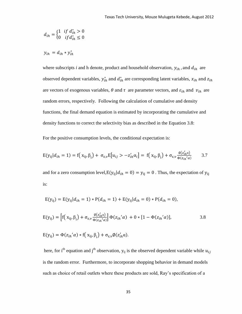
where subscripts i and h denote, product and household observation, are
observed dependent variables,
are corresponding latent variables,
are vectors of exogenous variables, are parameter vectors, and are
random errors, respectively. Following the calculation of cumulative and density
functions, the final demand equation is estimated by incorporating the cumulative and
density functions to correct the selectivity bias as described in the Equation 3.8:
For the positive consumption levels, the conditional expectation is:
3.7
and for a zero consumption level, . Thus, the expectation of
is:
3.8
here, for ith
equation and jth
observation, yij is the observed dependent variable while
is the random error. Furthermore, to incorporate shopping behavior in demand models
such as choice of retail outlets where these products are sold, Ray’s specification of a

Texas Tech University, Mouze Mulugeta Kebede, August 2012
36
‘basic’ equivalence scale was used. The scales were normalized at unity for a household
that shops at non-chain or independent stores. The equivalence scale used here is constant
across price distributions and utility levels, thus the modified system with shopping
behavior incorporated is theoretically feasible given that the original model is feasible.
Starting from a household expenditure function in terms of a reference expenditure
function that represents a household who shops from independent stores, a given
household expenditure can be specified as:
3.9
where is the cost function for the reference household, is a general
equivalence scale formulated as where and are retail
choice by households and their coefficients, respectively. Respective demand forms
(LES, AIDS, and LINQUAD) in the second stage with inclusion of demographic
variables and product attributes are discussed below. Pollak and Wales (1992) modified
LES specification in budget share form as:
for home-textiles, and
for apparel 3.10
where the p’s denote prices, M denotes total textile expenditure, ‘s denotes the
translating demographic variable, w’s denote the budget share devoted to good i and
Texas Tech University, Mouze Mulugeta Kebede, August 2012
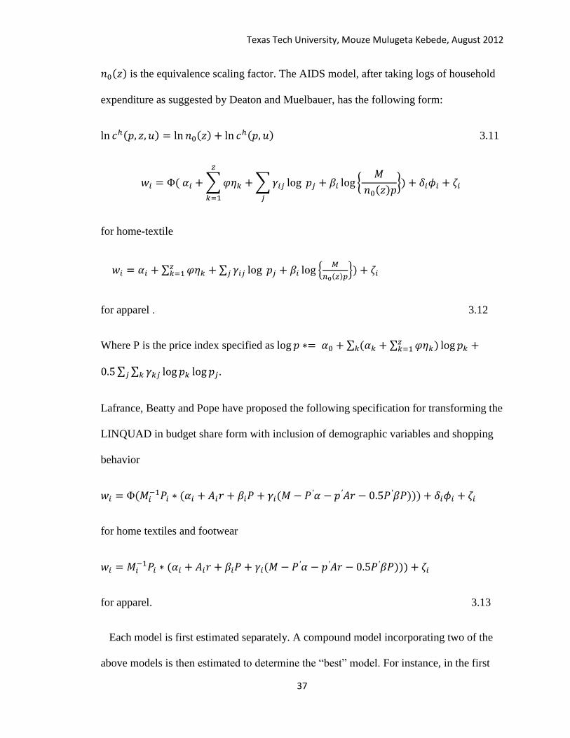
37
is the equivalence scaling factor. The AIDS model, after taking logs of household
expenditure as suggested by Deaton and Muelbauer, has the following form:
3.11
for home-textile
for apparel . 3.12
Where P is the price index specified as
.
Lafrance, Beatty and Pope have proposed the following specification for transforming the
LINQUAD in budget share form with inclusion of demographic variables and shopping
behavior
for home textiles and footwear
for apparel. 3.13
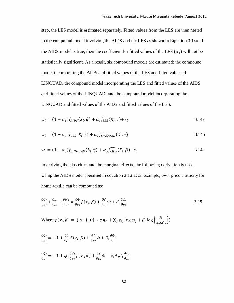
Each model is first estimated separately. A compound model incorporating two of the
above models is then estimated to determine the “best” model. For instance, in the first
Texas Tech University, Mouze Mulugeta Kebede, August 2012
38
step, the LES model is estimated separately. Fitted values from the LES are then nested
in the compound model involving the AIDS and the LES as shown in Equation 3.14a. If
the AIDS model is true, then the coefficient for fitted values of the LES ( ) will not be
statistically significant. As a result, six compound models are estimated: the compound
model incorporating the AIDS and fitted values of the LES and fitted values of
LINQUAD, the compound model incorporating the LES and fitted values of the AIDS
and fitted values of the LINQUAD, and the compound model incorporating the
LINQUAD and fitted values of the AIDS and fitted values of the LES:
3.14a
3.14b
3.14c
In deriving the elastcities and the marginal effects, the following derivation is used.
Using the AIDS model specified in equation 3.12 as an example, own-price elasticity for
home-textile can be computed as:
3.15
Where

Texas Tech University, Mouze Mulugeta Kebede, August 2012
39
Here refers to the first step (probit) equation of the estimation process.
3.3 Data Source and Description
The data used for this analysis is obtained from a 2009 cotton consumer tracking study
conducted by Cotton Council International through a local market research firm in China.
In total, a survey response from 6532 households in 24 cities from 4 waves is used for
this analysis. The main content of the survey is based on household heads ages 15-54 that
lived in the city for at least one year. The data set includes extensive household
demographic profile information associated with textile consumption, quantities, and
prices. In total, there are 1,378 variables describing each household.
The data on textile consumption for households in the survey are aggregated into three
categories: apparel, home textiles, and footwear. Here, the data set used has some zero
observations for quantity consumed and prices for items not consumed by a particular
household. To estimate a complete system, however, observations on prices for all goods
for all households must be available. A regression model is used to impute data for
missing prices. That is, prices for those households consuming each textile product are
regressed on household characteristics and regional dummies. The regression is then used
to estimate the missing prices for households with corresponding explanatory variables
but who were not consuming the textile product. Demographic variables used include
household income, age, occupation, education, and sex of the household head, and
household size.

Texas Tech University, Mouze Mulugeta Kebede, August 2012
40
During 2009, apparel is purchased by nearly all households (99.68%), footwear is
purchased by over 75.5% of the households, and only 38% of the households made a
purchase of home textiles. Table 3.1 provides a descriptive statistics of the data used in
the analysis. On basis of average prices, home textiles are the least expensive; while
apparel has the highest price variability and is the most purchased. A majority of
households (71.56%) in the sample have a monthly income in the range below 5000
Yuan ($793) and have a family size over two people (78%) as shown in Table 3.2. Over
70% of the sampled households have completed primary school, and over 65% of the
sampled households belong to the young demographic group (aged between 20-40). Also
from the data set, most of the sampled households (33%) shop for their textile and shoe
products from department stores. Over one third of sampled households have reported
having children of a younger age (<15 years of age), while over 16% of the sampled
households have reported having an adult over age 55 in their home.

Texas Tech University, Mouze Mulugeta Kebede, August 2012
41
Table 3.1. Descriptive statistics on apparel, textile and footwear consumption for Chinese
urban households, CCI survey, 2009.
Variable Mean Standard
Deviation
Quantity
Apparel (consuming households: 99.69% of the sample)
Textile (consuming households: 38% of the sample)
Foot wear(consuming households: 75% of the sample)
5.2381
1.0346
0.9984
4.9068
1.7743
0.8202
Retail price
Apparel
Home Textile
Foot wear
56.0995
27.8487
58.8522
63.6815
36.8369
48.1609
Expenditure (Yuan per household per year)
Apparel
Home textile
Footwear
361.8202
260.1946
35.7408
65.8847
562.5819
419.4281
201.5575
127.2654
Budget share
Apparel
Home Textile
Foot wear
0.7359
0.0667
0.1973
0.2088
0.1295
0.1859

Texas Tech University, Mouze Mulugeta Kebede, August 2012
42
Table 3.2. Frequency distribution of household demographic characteristics (sample size:
6532)
Description Categories Frequency Percentage
Age of household
head
Less than 20
20-29
30-39
40-49
Over 50
461
2046
1783
1541
701
7.06
31.32
27.30
23.59
10.73
Education ≤Primary
Junior, Technical &high school
College and over
1939
655
3938
29.68
10.03
60.29
Income < 5000 Yuan
5000-10000 Yuan
10000-15000 Yuan
Over15000 Yuan
4674
1586
204
68
71.56
24.28
3.12
1.04
Gender Male
Female
2622
3910
40.14
59.86
Retail
choice(apparel)
Department store
Chain and specialty stores
Warehouse
Small Independent (non-chain,
tailor made)
Others(discount stores, internet,
factory outlet, TV home
shopping, door to door, bazaars)
2833
2185
487
652
375
43.37
33.45
7.46
9.98
5.74

Texas Tech University, Mouze Mulugeta Kebede, August 2012
43
Table 3.2. Frequency distribution of household demographic characteristics (sample size:
6532) continued....
Retail choice (home
textile)
Department store
Chain and specialty stores
Warehouse
Small Independent (non-chain)
Others(discount stores, internet,
factory outlet, TV home
shopping, door to door, bazaars,
none)
2062
790
902
278
2500
31.57
12.09
13.81
4.26
38.27
Retail choice
(footwear)
Department store
Chain and specialty stores
Warehouse
Small Independent (non-chain)
Others(discount stores, internet,
sporting stores, factory outlet, TV
home shopping, door to door,
bazaars)
2725
2629
375
386
417
41.72
40.25
5.74
5.91
6.38
Household size Less or equal to 2
3-5
Over 6
1397
4929
206
21.38
75.46
3.17
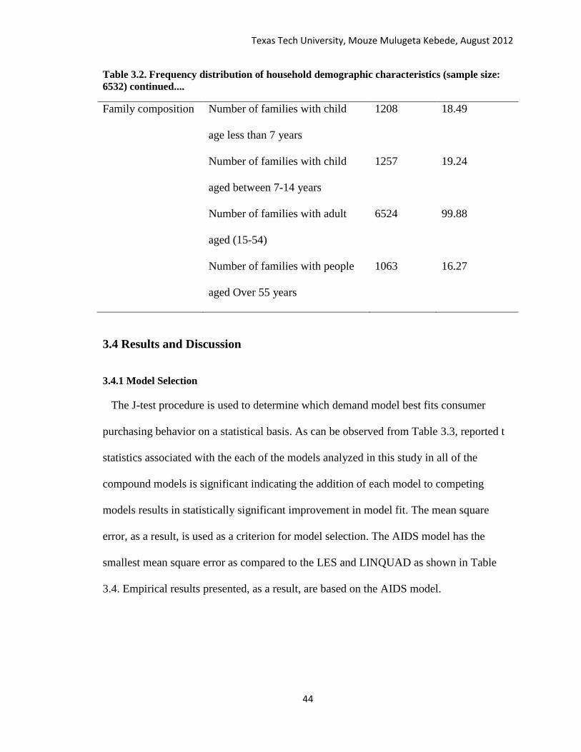
Texas Tech University, Mouze Mulugeta Kebede, August 2012
44
Table 3.2. Frequency distribution of household demographic characteristics (sample size:
6532) continued....
Family composition
Number of families with child
age less than 7 years
Number of families with child
aged between 7-14 years
Number of families with adult
aged (15-54)
Number of families with people
aged Over 55 years
1208
1257
6524
1063
18.49
19.24
99.88
16.27
3.4 Results and Discussion
3.4.1 Model Selection
The J-test procedure is used to determine which demand model best fits consumer
purchasing behavior on a statistical basis. As can be observed from Table 3.3, reported t
statistics associated with the each of the models analyzed in this study in all of the
compound models is significant indicating the addition of each model to competing
models results in statistically significant improvement in model fit. The mean square
error, as a result, is used as a criterion for model selection. The AIDS model has the
smallest mean square error as compared to the LES and LINQUAD as shown in Table
3.4. Empirical results presented, as a result, are based on the AIDS model.
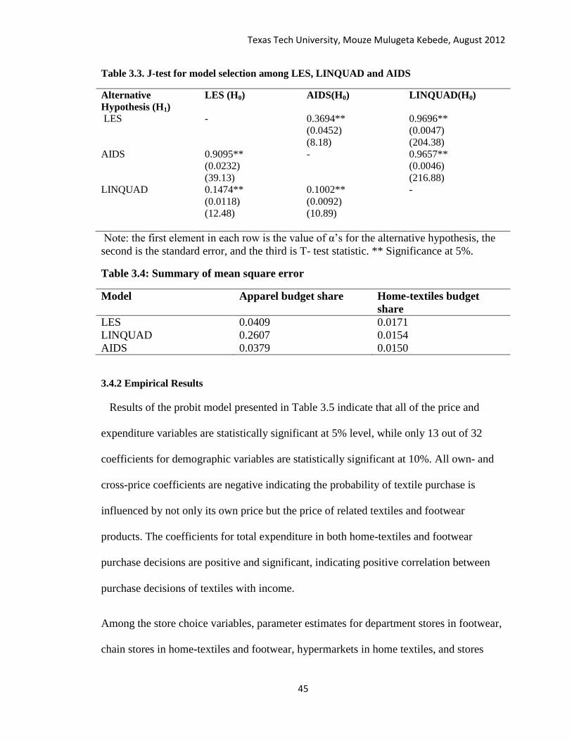
Texas Tech University, Mouze Mulugeta Kebede, August 2012
45
Table 3.3. J-test for model selection among LES, LINQUAD and AIDS
Alternative
Hypothesis (H1)
LES (H0) AIDS(H0) LINQUAD(H0)
LES - 0.3694**
(0.0452)
(8.18)
0.9696**
(0.0047)
(204.38)
AIDS 0.9095**
(0.0232)
(39.13)
- 0.9657**
(0.0046)
(216.88)
LINQUAD 0.1474**
(0.0118)
(12.48)
0.1002**
(0.0092)
(10.89)
-
Note: the first element in each row is the value of ’s for the alternative hypothesis, the
second is the standard error, and the third is T- test statistic. ** Significance at 5%.
Table 3.4: Summary of mean square error
Model Apparel budget share Home-textiles budget
share
LES 0.0409 0.0171
LINQUAD 0.2607 0.0154
AIDS 0.0379 0.0150
3.4.2 Empirical Results
Results of the probit model presented in Table 3.5 indicate that all of the price and
expenditure variables are statistically significant at 5% level, while only 13 out of 32
coefficients for demographic variables are statistically significant at 10%. All own- and
cross-price coefficients are negative indicating the probability of textile purchase is
influenced by not only its own price but the price of related textiles and footwear
products. The coefficients for total expenditure in both home-textiles and footwear
purchase decisions are positive and significant, indicating positive correlation between
purchase decisions of textiles with income.
Among the store choice variables, parameter estimates for department stores in footwear,
chain stores in home-textiles and footwear, hypermarkets in home textiles, and stores

Texas Tech University, Mouze Mulugeta Kebede, August 2012
46
under the “others” category in home-textiles are all statistically significant. Effects of
shopping behavior such as the decision of where to purchase textile products indicated
that the probability of home-textile purchase is positively related to chain stores and
hyper-markets, while the probability of home-textiles purchase is inversely related to
stores categorized under the “others”. A purchase decision of footwear, on other hand, is
positively related to department stores and chain stores.
Table 3.5. Estimated parameters of participation equation for home textiles and footwear
participation equation parameters Home textile Footwear
Intercept
Apparel price
0.3476**
-0.0045**
0.4789**
-0.0039**
Home textile price -0.0038** -0.0064**
Footwear price -0.0029** -0.0027**
Income 0.0011** 0.0017**
Age 15-29(reference over50) -0.0550 0.1966**
Age 30-39 0.0653 0.1032
Age 40-49 0.0203 0.0231
Single -0.1651** 0.1159*
Divorced/widowed 0.0876 0.0395
Technical, junior, high school(reference Primary education) 0.0420 0.0555
College and over 0.0779* 0.1104**
Gender(reference female) -0.5363** 0.0170
Department store(reference independent store) 0.1194 0.1278*
Chain/specialty store 0.2147** 0.1449*
Warehouse 0.2275** 0.0949

Texas Tech University, Mouze Mulugeta Kebede, August 2012
47
Table 3.5. Estimated parameters of participation equation for home textiles and footwear
(continued...)
Others stores -1.1288** 0.0172
Child less than 7 year old(reference age b/n 15-54) -0.1053* -0.1369**
Child between 7-15 -0.0510 -0.0348
Old over age 55 0.0477 -0.0513
Family size -0.0302 -0.0105
Note: * indicates significance at 10% level while ** significance at 5% level
Effects of demographic variables on purchase decisions were also estimated. Results
indicate that the probability of home-textiles purchase is lower if the household head is a
man, is single, or has a child less than 7 years old. Footwear purchase probablity, on the
other hand, is positively related to household heads in the age group 15-29, to single
households, or to household heads who finished some college education, while it is lower
in households with a younger child (aged less than 7 years).
Results from the probit model are used to calculate the inverse Mills ratio that is
incorporated in the structural component of the model. Table 3.6 presents parameter
estimates for the AIDS model. Theoretical restrictions of homogeneity and symmetry are
maintained during estimation, but the theoretical restriction of adding up on parameter
estimates, in general, does not hold as is the case in many demand studies using the AIDS
model. As a result, estimation on budget equations is made by treating the footwear
category as a residual good as suggested by Yen, Lin, and Smallwood and estimating n-1
equations with an identity . Many of the coefficients on demographic
variables are not statistically significant. Own-price, cross-price, and total expenditure
coefficients are all statistically significant. In regards to shopping behavior such as retail
choice, only the coefficient for the“others” store is significant. This result, in turn,

Texas Tech University, Mouze Mulugeta Kebede, August 2012
48
indicates that under price invariance of the scale, households who often purchase from
locations categorized under “others”, which includes bazaars, discount stores, internet
purchases, and factory outlets, have lower expense for apparel products when compared
to households who purchase from independent, department, and chain stores. Households
who often purchase from chain, department and independent stores also have a lower
expense on home-textiles when compared to customers who buy from stores under the
“others” category.
Table 3.6. AIDS parameter estimates
Variables Apparel Home textile
Intercept 0.8820** -0.0440
(0.0382) (0.0522)
Age 15-29 (ref:over50) 0.0171 -0.0776**
(0.0314) (0.039)
Age 30-39 0.0144 -0.0192
(0.0364) (0.0450)
Age 40-49 -0.0170
(0.0328)
0.0321
(0.0404)
Technical, junior, high school ( ref: Primary education) -0.0275 0.0091
(0.0415) (0.0517)
College and over 0.0099 -0.0376
(0.0229) (0.0275)
Child less than 7 year old( ref: no dependent) 0.0061 0.0355
(0.0283) (0.0349)

Texas Tech University, Mouze Mulugeta Kebede, August 2012
49
Table 3.6. AIDS parameter estimates (continued...)
Child between 7-15 0.0664** -0.0720**
(0.0294) (0.0366)
Old over age 50 -0.0101 0.0218
(0.0276) (0.0342)
Gender(ref: female) -0.0608** 0.0165
(0.0209) (0.0261)
Family size 0.0043 -0.0017
(0.0096) (0.0112)
Home textile price -0.0054** 0.0464**
(0.0025) (0.0038)
Apparel price 0.0521 ** -0.0054**
(0.0035) (0.0025)
Expenditure -0.0492** 0.0608**
(0.0030) (0.004)
Department store 0.0591 0.4340
(0.3760)
(0.1650)
Chain store 0.0352 0.1821
(0.3345)
(0.1661)
Warehouse -0.0753 0.0461
(0.1954) (0.2926)
Others stores -0.3493** 3.3160**
(0.1501) (1.2408)
Note: * indicates significance at 10% level while ** significance at 5% level
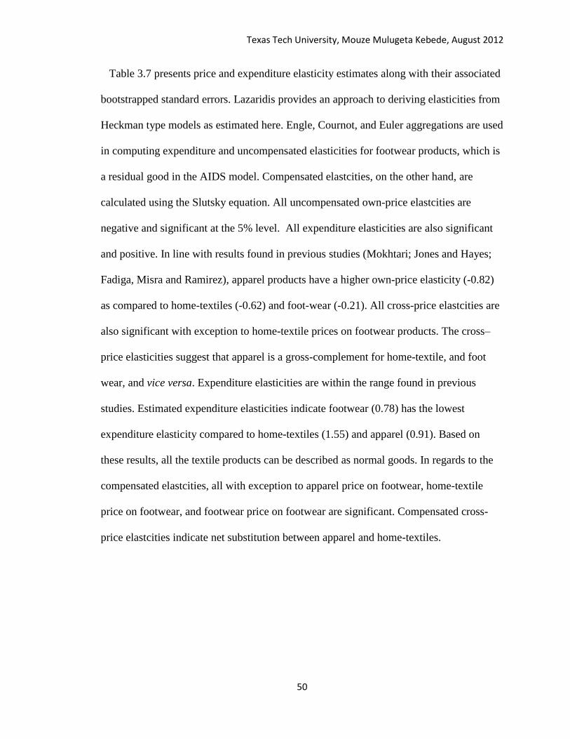
Texas Tech University, Mouze Mulugeta Kebede, August 2012
50
Table 3.7 presents price and expenditure elasticity estimates along with their associated
bootstrapped standard errors. Lazaridis provides an approach to deriving elasticities from
Heckman type models as estimated here. Engle, Cournot, and Euler aggregations are used
in computing expenditure and uncompensated elasticities for footwear products, which is
a residual good in the AIDS model. Compensated elastcities, on the other hand, are
calculated using the Slutsky equation. All uncompensated own-price elastcities are
negative and significant at the 5% level. All expenditure elasticities are also significant
and positive. In line with results found in previous studies (Mokhtari; Jones and Hayes;
Fadiga, Misra and Ramirez), apparel products have a higher own-price elasticity (-0.82)
as compared to home-textiles (-0.62) and foot-wear (-0.21). All cross-price elastcities are
also significant with exception to home-textile prices on footwear products. The cross–
price elasticities suggest that apparel is a gross-complement for home-textile, and foot
wear, and vice versa. Expenditure elasticities are within the range found in previous
studies. Estimated expenditure elasticities indicate footwear (0.78) has the lowest
expenditure elasticity compared to home-textiles (1.55) and apparel (0.91). Based on
these results, all the textile products can be described as normal goods. In regards to the
compensated elastcities, all with exception to apparel price on footwear, home-textile
price on footwear, and footwear price on footwear are significant. Compensated cross-
price elastcities indicate net substitution between apparel and home-textiles.
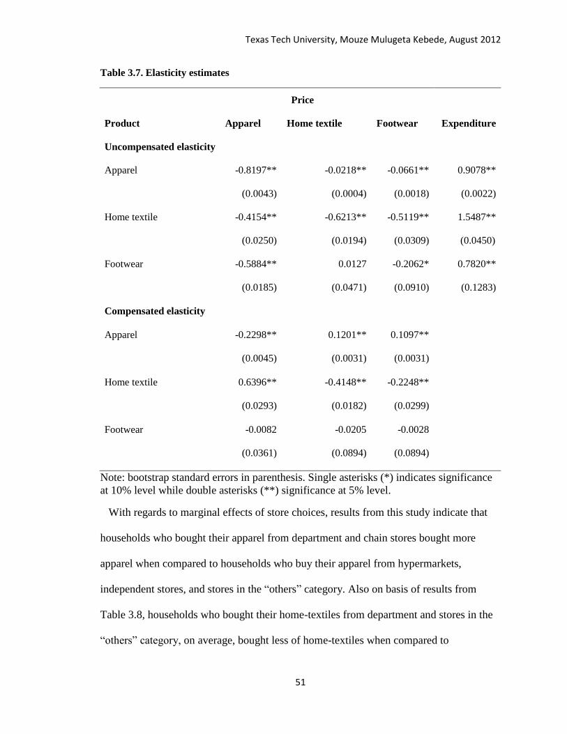
Texas Tech University, Mouze Mulugeta Kebede, August 2012
51
Table 3.7. Elasticity estimates
Price
Expenditure
Product Apparel Home textile Footwear
Uncompensated elasticity
Apparel
-0.8197**
(0.0043)
-0.0218**
(0.0004)
-0.0661**
(0.0018)
0.9078**
(0.0022)
Home textile
-0.4154**
(0.0250)
-0.6213**
(0.0194)
-0.5119**
(0.0309)
1.5487**
(0.0450)
Footwear
-0.5884**
(0.0185)
0.0127
(0.0471)
-0.2062*
(0.0910)
0.7820**
(0.1283)
Compensated elasticity
Apparel
-0.2298**
(0.0045)
0.1201**
(0.0031)
0.1097**
(0.0031)
Home textile
0.6396**
(0.0293)
-0.4148**
(0.0182)
-0.2248**
(0.0299)
Footwear
-0.0082
(0.0361)
-0.0205
(0.0894)
-0.0028
(0.0894)
Note: bootstrap standard errors in parenthesis. Single asterisks (*) indicates significance
at 10% level while double asterisks (**) significance at 5% level.
With regards to marginal effects of store choices, results from this study indicate that
households who bought their apparel from department and chain stores bought more
apparel when compared to households who buy their apparel from hypermarkets,
independent stores, and stores in the “others” category. Also on basis of results from
Table 3.8, households who bought their home-textiles from department and stores in the
“others” category, on average, bought less of home-textiles when compared to
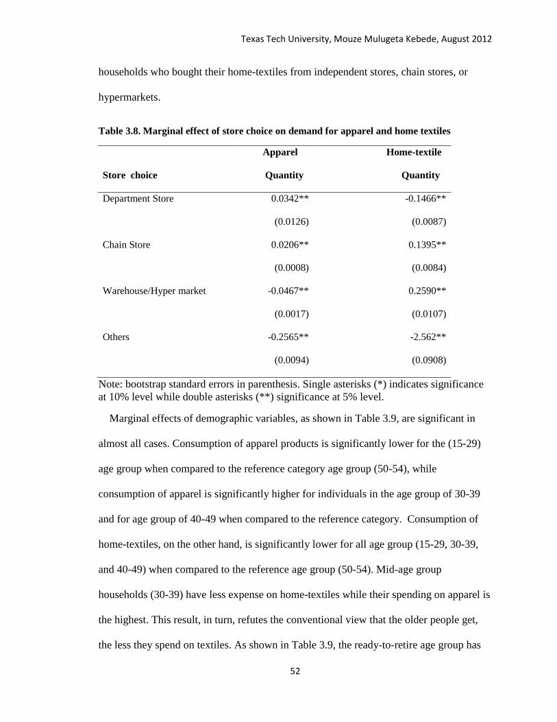
Texas Tech University, Mouze Mulugeta Kebede, August 2012
52
households who bought their home-textiles from independent stores, chain stores, or
hypermarkets.
Table 3.8. Marginal effect of store choice on demand for apparel and home textiles
Apparel Home-textile
Store choice Quantity Quantity
Department Store 0.0342** -0.1466**
(0.0126) (0.0087)
Chain Store 0.0206** 0.1395**
(0.0008) (0.0084)
Warehouse/Hyper market -0.0467** 0.2590**
(0.0017) (0.0107)
Others -0.2565** -2.562**
(0.0094) (0.0908)
Note: bootstrap standard errors in parenthesis. Single asterisks (*) indicates significance
at 10% level while double asterisks (**) significance at 5% level.
Marginal effects of demographic variables, as shown in Table 3.9, are significant in
almost all cases. Consumption of apparel products is significantly lower for the (15-29)
age group when compared to the reference category age group (50-54), while
consumption of apparel is significantly higher for individuals in the age group of 30-39
and for age group of 40-49 when compared to the reference category. Consumption of
home-textiles, on the other hand, is significantly lower for all age group (15-29, 30-39,
and 40-49) when compared to the reference age group (50-54). Mid-age group
households (30-39) have less expense on home-textiles while their spending on apparel is
the highest. This result, in turn, refutes the conventional view that the older people get,
the less they spend on textiles. As shown in Table 3.9, the ready-to-retire age group has
Texas Tech University, Mouze Mulugeta Kebede, August 2012
53
the highest expense on home-textiles when compared to all the age groups and appears to
have a higher apparel expense than the young age group (15-29). Another important
demographic variable explaining consumption patterns in apparel and home-textiles is
family composition. As reported in Table 3.9, the presence of a child aged less than 15 in
a household increases apparel consumption and decreases home-textile consumption.
Similarly, households with an elderly member (aged over 50) consume less apparel
products and spend more on home-textiles when compared to households with no
members in this age group. In general, households either headed by ready-to-retire age
group or having an elderly member appear to spend more on home-textiles than apparel
products, while households headed by mid-age group (30-39) or who have a child less
than seven years old appear to spend more on apparel than on home-textiles compared to
their counterparts. Consumption of apparel increases with increases in head of household
education level, while consumption of home-textiles declines with increase in education
level of the household head. Men headed households consume less apparel and home-
textiles when compared to female headed households. Family size, on the other hand, has
an inverse effect on home textiles and positive and significant effect on apparel
consumption. The inverse effect of family size on home textiles is consistent with
previous results such as those reported by Wagner and Mokharti. They indicated that
such results are possible either because of operation of economies of scale in large
families or the need for other necessities such as food, thus forcing them to allocate less
for home-textiles.
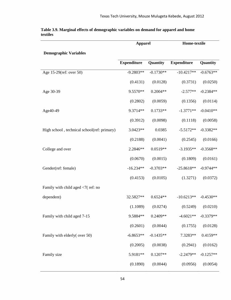
Texas Tech University, Mouze Mulugeta Kebede, August 2012
54
Table 3.9. Marginal effects of demographic variables on demand for apparel and home
textiles
Demographic Variables
Apparel
Home-textile
Expenditure Quantity Expenditure Quantity
Age 15-29(ref: over 50) -9.2803** -0.1730** -10.4217** -0.6763**
(0.4131) (0.0128) (0.3731) (0.0250)
Age 30-39 9.5570** 0.2004** -2.577** -0.2384**
(0.2802) (0.0059) (0.1356) (0.0114)
Age40-49 9.3714** 0.1733** -1.3771** -0.0410**
(0.3912) (0.0098) (0.1118) (0.0058)
High school , technical school(ref: primary) 3.0423** 0.0385 -5.5172** -0.3382**
(0.2188) (0.0041) (0.2545) (0.0166)
College and over 2.2846** 0.0519** -3.1935** -0.3568**
(0.0670) (0.0015) (0.1809) (0.0161)
Gender(ref: female) -16.234** -0.3703** -25.8618** -0.9744**
(0.4153) (0.0105) (1.3271) (0.0372)
Family with child aged <7( ref: no
dependent) 32.5827** 0.6524** -10.6213** -0.4530**
(1.1089) (0.0274) (0.5249) (0.0210)
Family with child aged 7-15 9.5884** 0.2409** -4.6021** -0.3379**
(0.2601) (0.0044) (0.1755) (0.0128)
Family with elderly( over 50) -6.8653** -0.1435** 7.3283** 0.4159**
(0.2005) (0.0038) (0.2941) (0.0162)
Family size 5.9181** 0.1207** -2.2479** -0.1257**
(0.1890) (0.0044) (0.0956) (0.0054)
Texas Tech University, Mouze Mulugeta Kebede, August 2012
55
3.5 Summary and Conclusion
This study has compared three demand systems for estimating the Chinese household
textile demand structure. On basis of the mean-square error, the AIDS specification
provides the best approximation of Chinese textile consumption patterns in statistical
terms. Results from this study indicate that the price of products and household income
affect both decisions to participate in the textile market and quantity of textiles
purchased. Shopping behavior such as consumer’s decision of where to buy also plays a
role in household participation decisions in the home-textile market and in budget
allocation of apparel and home-textiles. Accordingly, department stores are most likely to
be successful if they target apparel products. But, these stores are less attractive in selling
home-textile products when compared to chain stores and hypermarkets.
In regards to demographic variables, women of middle age group (30-39), or
household heads who completed secondary education, or who have a younger child (aged
less than seven) in their family have the largest apparel expense while women who are
over the age of 50, or household heads who have only a primary education, or who have
an elderly member in their household have the largest home-textile expense as compared
to any other demographic group
All the products considered here are more likely to be purchased with increases in
income. Applying income elasticity estimates from Table 3.7, and a per capita income
growth rate of 10 percent per year, Chinese consumers are expected to increase their
textile spending at least by 8 percent every year. Such growth in textile spending by
Chinese consumers, given a per capita income of $4210 according to World Bank recent
Texas Tech University, Mouze Mulugeta Kebede, August 2012
56
estimates, could amount in aggregate to over $29 billion each year highlighting the
potential for growth of the Chinese textile market.
In conclusion, though the Chinese population is growing old and declining in growth
rate, the negative effect as a result of demographic changes on textile demand could be
overshadowed if China is able to sustain its current economic growth rate. Considering
the low rate of current fiber consumption when compared to the developed world and a
relatively high income elasticity, results obtained from this study, suggest the potential
for expansion of textile markets in China is promising.

Texas Tech University, Mouze Mulugeta Kebede, August 2012
57
Chapter Four
Demand for Apparel Products among Chinese Consumers Using a
Semi-parametric Two Step Procedure
Introduction
China, with its growing population and rising per capita income, has become an
attractive market for apparel products. Many foreign brands and retailers are entering this
market, given its huge potential. To capture a bigger share of this market, however,
requires an understanding of consumers’ taste and selection criteria in purchase
decision making. While the previous chapter provides useful information about aggregate
textile demand, the information needed for specific product marketing decision is less
likely to be acquired from analysis of aggregate commodities. Decision makers who often
are involved with new product developments and advertising, thus, require information
on actual product purchase. Such information helps, for instance, in designing their
marketing strategies; which includes, but is not limited to, understanding of the effects of
quality attributes, store characteristics, relative prices and consumers’ socio-economic
profiles. Despite such benefits, examination of individual product demand is often
complicated owing to zero consumption levels of the various products by many
households. Use of conventional demand models without accounting for the zero
observations will result in biased parameter estimates (Amemiya, 1984).
To account for the positive probability of zero consumption, two approaches are
commonly used: a Tobin type censored regression model and a two-step procedure
proposed by Heckman. The Heckman two-step procedure for household demand,
Texas Tech University, Mouze Mulugeta Kebede, August 2012
58
proposed by Heien and Wessell and extended by Shonkwiler and Yen, requires the
computation of a probit model as a first step to analyze the decision of whether or not to
purchase the good. In the second step, expenditure shares are augmented with a “Mills
Ratio” regressor to account for the censoring, or more, specifically, the probability that a
household does not consume that product.
Despite wide use of parametric censored demand models in empirical research, results
from such models are often criticized for being sensitive to the assumed parametric
distribution of the error terms. In parametric models, one cannot immediately detect
whether measurements are driven by data or by the imposed parametric functional forms
- where the functional form of the relationship is predetermined. In addition, more often
than not, the distribution of the latent variable error is unknown and thus may be related
to the regressors leading to conditional heteroscedastcity problems of an unknown form
(Yen and Lin). According to Hurd, in cases where errors from a latent regression are
heteroscedastic, regression based on the homoscedastic assumption is likely to result in
inconsistent estimates. Yet, a non-parametric approach also has its own flaws. Given the
limited structure of such estimation techniques, inference based on such estimation
techniques is often very limited (Greene). That is, estimates from a nonparametric
approach are difficult to interpret and the only result that one can infer from such analysis
is an estimate of the density function. A semi-parametric approach, on the other hand,
serves as a bridge between the two approaches and has an advantage over the parametric
approach in cross sectional analysis because it relies less on assumptions such as
normality and homoscedasticity. Given such advantages, non-parametric smoothing
methods have been used in applied demand analysis studies by Sam and Zheng, and
Texas Tech University, Mouze Mulugeta Kebede, August 2012
59
Belasco, Ghosch, and Chidmi. Because consumption data patterns behave nonlinearly in
relation to demographic variables and to prices, this study aims to exploit the advantages
of a semi-parametric approach; here, the study intends to implement a semi-parametric
approach to analyze effects of changes in Chinese demographic structure on apparel
demand. Furthermore, given the increasing taste for cotton among Chinese consumers in
recent years (Qui, 2005), this analysis explores whether choice of fiber content of apparel
products affects in the consumption of apparel.
4.1 Conceptual Framework
Estimating a complete demand system derived from pure neoclassical theory is often
difficult because it requires large quantities of data. The usual method of addressing such
a problem is to assume some form of a structure of consumer preferences. Here, the study
uses a three stage budgeting procedure which allows households to allocate total
expenditure in sequential stages.
For this study, the first stage involves income allocation between textile and non-textile
products. The first stage of the demand relation is not estimated in this study as the data
collected doesn’t provide information on expense made by households on non-textile
products. The study uses the weak seperability assumption to overcome data limitation
problems of non-textile consumption. In the second stage, a demand system is specified
for three sub group of textiles and footwear: home-textiles, apparel, and footwear. In the
third stage, a demand system for apparel products is specified consisting of shirts, coats
and suits, dresses, pants, and “other” clothing products.
At the first stage of the three stage allocation process, there are N commodity groups
where one of these commodities is textiles and footwear as shown in Figure 4.1. The
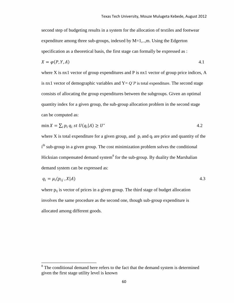
Texas Tech University, Mouze Mulugeta Kebede, August 2012
60
second step of budgeting results in a system for the allocation of textiles and footwear
expenditure among three sub-groups, indexed by M=1,..,m. Using the Edgerton
specification as a theoretical basis, the first stage can formally be expressed as :
4.1
where X is nx1 vector of group expenditures and P is nx1 vector of group price indices, A
is nx1 vector of demographic variables and Y= Q’P is total expenditure. The second stage
consists of allocating the group expenditures between the subgroups. Given an optimal
quantity index for a given group, the sub-group allocation problem in the second stage
can be computed as:
4.2
where X is total expenditure for a given group, and pi and qi are price and quantity of the
ith
sub-group in a given group. The cost minimization problem solves the conditional
Hicksian compensated demand system8 for the sub-group. By duality the Marshalian
demand system can be expressed as:
4.3
where pij is vector of prices in a given group. The third stage of budget allocation
involves the same procedure as the second one, though sub-group expenditure is
allocated among different goods.
8 The conditional demand here refers to the fact that the demand system is determined
given the first stage utility level is known
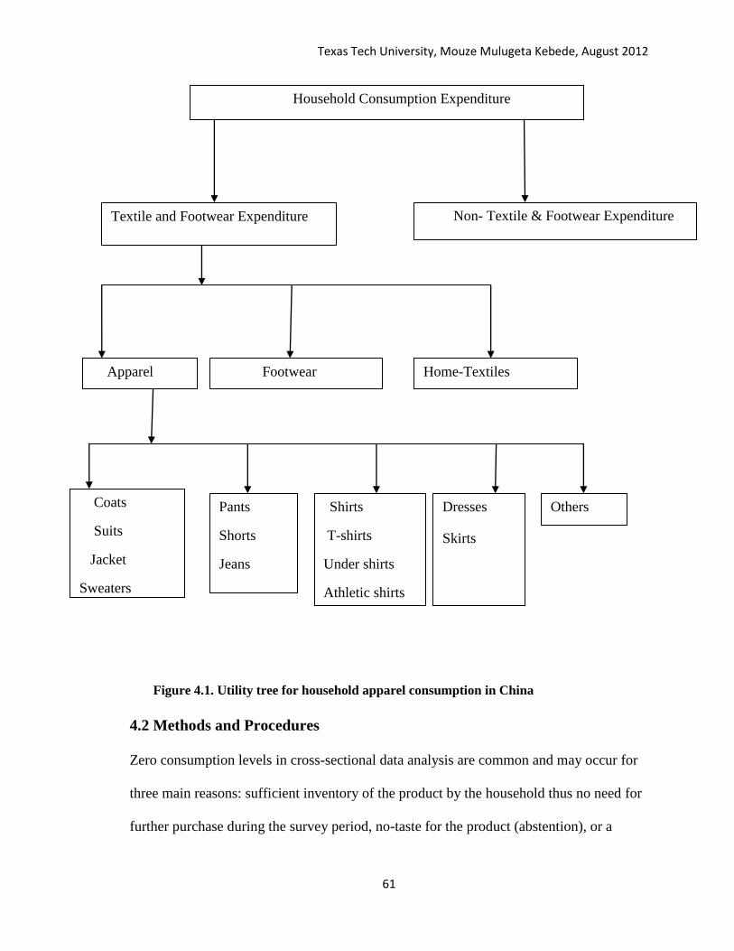
Texas Tech University, Mouze Mulugeta Kebede, August 2012
61
4.2 Methods and Procedures
Zero consumption levels in cross-sectional data analysis are common and may occur for
three main reasons: sufficient inventory of the product by the household thus no need for
further purchase during the survey period, no-taste for the product (abstention), or a
Household Consumption Expenditure
Textile and Footwear Expenditure Non- Textile & Footwear Expenditure
Apparel Footwear Home-Textiles
Coats
Suits
Jacket
Sweaters
Pants
Shorts
Jeans
Shirts
T-shirts
Under shirts
Athletic shirts
Dresses
Skirts
Others
Figure 4.1. Utility tree for household apparel consumption in China
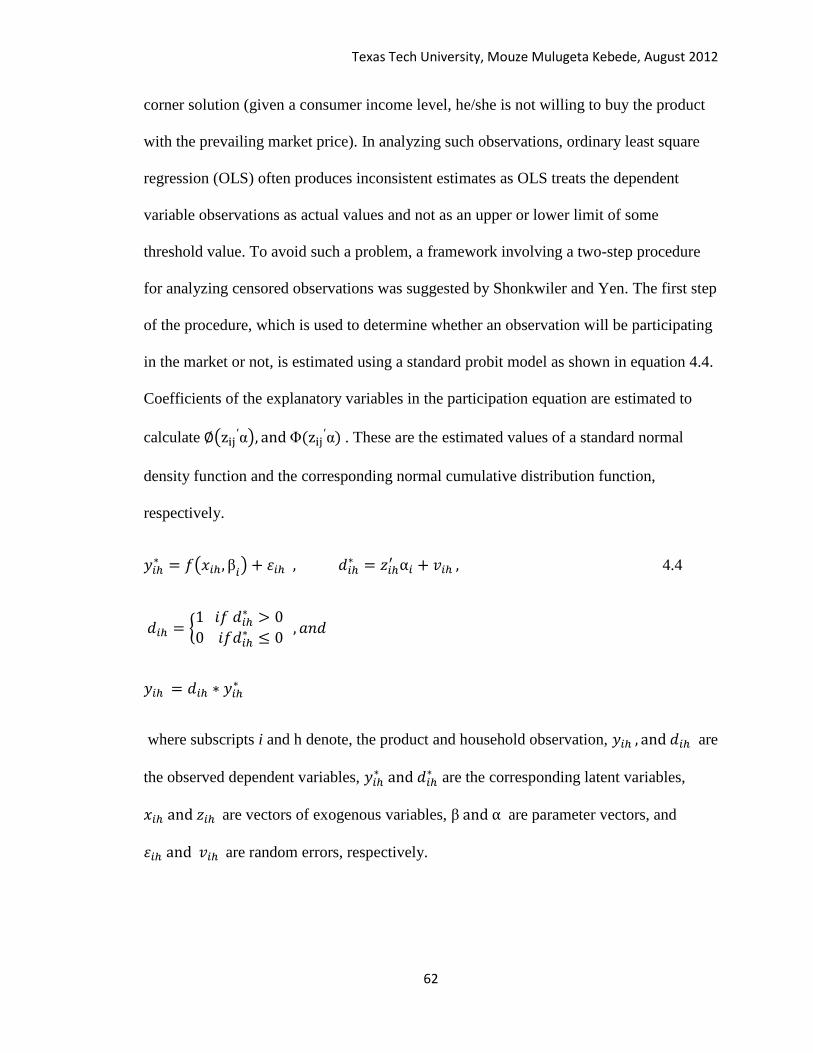
Texas Tech University, Mouze Mulugeta Kebede, August 2012
62
corner solution (given a consumer income level, he/she is not willing to buy the product
with the prevailing market price). In analyzing such observations, ordinary least square
regression (OLS) often produces inconsistent estimates as OLS treats the dependent
variable observations as actual values and not as an upper or lower limit of some
threshold value. To avoid such a problem, a framework involving a two-step procedure
for analyzing censored observations was suggested by Shonkwiler and Yen. The first step
of the procedure, which is used to determine whether an observation will be participating
in the market or not, is estimated using a standard probit model as shown in equation 4.4.
Coefficients of the explanatory variables in the participation equation are estimated to
calculate
. These are the estimated values of a standard normal
density function and the corresponding normal cumulative distribution function,
respectively.
4.4
where subscripts i and h denote, the product and household observation, are
the observed dependent variables,
are the corresponding latent variables,
are vectors of exogenous variables, are parameter vectors, and
are random errors, respectively.

Texas Tech University, Mouze Mulugeta Kebede, August 2012
63
Following the calculation of the cumulative and density functions, the final demand
equation is estimated by incorporating the cumulative and density functions to correct the
selectivity bias as described in Equation4.6:
For the positive consumption levels, the conditional expectation is:
4.5
and for a zero consumption level, . Thus, the expectation of
is:
4.6
Here, for ith
equation and jth
observation, yij is the observed dependent variable while
is the random error. Yet, the Shonkwiler and Yen approach (henceforth SY approach)
would yield consistent and unbiased estimates if the underlying distribution of the error
term is bi-variate normal. The study uses semi-parametric technique outlined by Newey,
Powell and Walker to circumvent possible misspecification and heteroscedasticity
problem in SY approach. In deriving the semi-parametric censored regression model, this
study uses the following specifications:
4.7
4.8

Texas Tech University, Mouze Mulugeta Kebede, August 2012
64
where I(.) is an indicator function,
9, and
are vectors of parameters. Using as the unknown cumulative distribution
function of the error term , the system of regression equations can be specified as:
4.9
where
. First will
be estimated using the Klien and Spady single index model, which is obtained by
maximizing the quasi-loglikelihood function:
4.10
where
and h is a smoothing parameter
satisfying the condition j-1/6
<h< j-1/8
. Location and scale parameterization requires setting
the intercept to zero and one of coefficients on a continuous explanatory variable to one.
Once estimates of are obtained using the Klein and Spady method, the
estimates will be incorporated to equation 4.9 to estimate the system of demand
equations. To estimate the unknown selectivity term , Newey, Powel and
Walker use a series approximation based on orthogonal polynomials,
i.e,
10 and k are allowed to increase with the
sample size. The system of equations can be estimated consistently as:
9 iid refers to the fact that errors terms from each observation are independent and are
identically distributed.
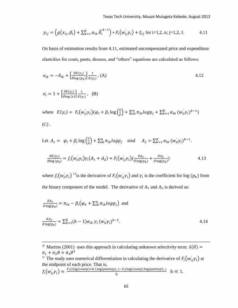
Texas Tech University, Mouze Mulugeta Kebede, August 2012
65
for i=1,2..n; j=1,2, J. 4.11
On basis of estimation results from 4.11, estimated uncompensated price and expenditure
elastcities for coats, pants, dresses, and “others” equations are calculated as follows:
, (A) 4.12
, (B)
where
(C) .
Let
.
4.13
where
11is the derivative of
and is the coefficient for from
the binary component of the model. The derivative of A1 and A2 is derived as:
and
. 4.14
10
Martins (2001) uses this approach in calculating unknown selectivity term:
11
The study uses numerical differentiation in calculating the derivative of at
the midpoint of each price. That is,

Texas Tech University, Mouze Mulugeta Kebede, August 2012
66
To find expenditure elasticity of dress (the residual commodity in the model),on the other
hand, the study used Engle aggregation. That is:
, 4.15
where are product price, quantity consumed, budget share, and total
expenditure, respectively. Euler aggregation is used to find the cross-price elasticity of
dress price on the other apparel products. That is:
4.16
At last, the study uses Cournot aggregation to calculate the cross-price effect of coat,
pants, shirts, and “others” price on dress.
4.17
Texas Tech University, Mouze Mulugeta Kebede, August 2012
67
The study uses the NP package, developed by Hayfield and Racine, under R software to
compute parameter estimates of the binary component of the model. For a non-parametric
model, estimates are obtained by slicing the data into different bins, then estimating the
behavior within the bin. The size of the bin is estimated using kernel density. Results
from the binary component then will be incorporated to the AIDS model to determine
households apparel consumption behavior.
4.3 Results and Discussion
The data used for this analysis were obtained from a 2009 cotton consumer tracking study
conducted by Cotton Council International through a local market research firm. In total,
a survey response from 2062 households in 24 cities from 2 waves was used for this
analysis. The main content of the survey is based on household heads ages15-54 who
lived in the city for at least one year. The data set includes extensive household
demographic information associated with apparel consumption, quantities, prices and
household expenditures on apparel products. In total, there are 1,378 variables describing
each household.
Due to the sparse nature of the dependent variables in the data set, products were
aggregated into five groups: suits and coats, shirts, pants, dresses, and “others” as shown
in Table 4.1. Still, the data set used has some missing observations on quantity consumed
and prices of the apparel products described above. Hence, a regression model is used to
impute the missing prices. That is, prices for those households consuming each apparel
product were regressed on household characteristics and regional dummies. The
regression was then used to estimate the missing prices for households who are not
consuming the apparel product. From the sampled data, 57 percent of the respondents
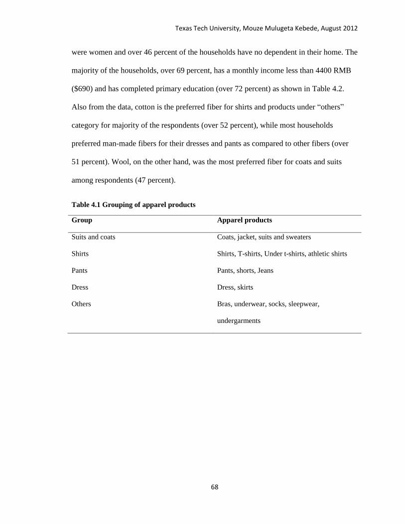
Texas Tech University, Mouze Mulugeta Kebede, August 2012
68
were women and over 46 percent of the households have no dependent in their home. The
majority of the households, over 69 percent, has a monthly income less than 4400 RMB
($690) and has completed primary education (over 72 percent) as shown in Table 4.2.
Also from the data, cotton is the preferred fiber for shirts and products under “others”
category for majority of the respondents (over 52 percent), while most households
preferred man-made fibers for their dresses and pants as compared to other fibers (over
51 percent). Wool, on the other hand, was the most preferred fiber for coats and suits
among respondents (47 percent).
Table 4.1 Grouping of apparel products
Group Apparel products
Suits and coats Coats, jacket, suits and sweaters
Shirts Shirts, T-shirts, Under t-shirts, athletic shirts
Pants Pants, shorts, Jeans
Dress Dress, skirts
Others Bras, underwear, socks, sleepwear,
undergarments

Texas Tech University, Mouze Mulugeta Kebede, August 2012
69
Table 4.2. Frequency distribution of respondents on basis of demographic characteristic
and product choice
Description Categories Frequency Percent
Fiber choice (pants) Cotton 532 25.80
Denim 90 4.36
Wool 12 0.58
Silk 3 0.15
Man-made 1274 61.78
Cotton blend 151 7.32
Fiber choice (shirts) Cotton 1084 52.57
Denim 7 0.34
Wool 13 0.63
Silk 14 0.68
Man-made 892 43.26
Cotton Blend 52 2.52
Fiber choice (dress) Cotton 391 18.96
Denim 75 3.64
Wool 81 3.93
Silk 330 16
Man-made 1061 51.45
Cotton Blend 124 6.01
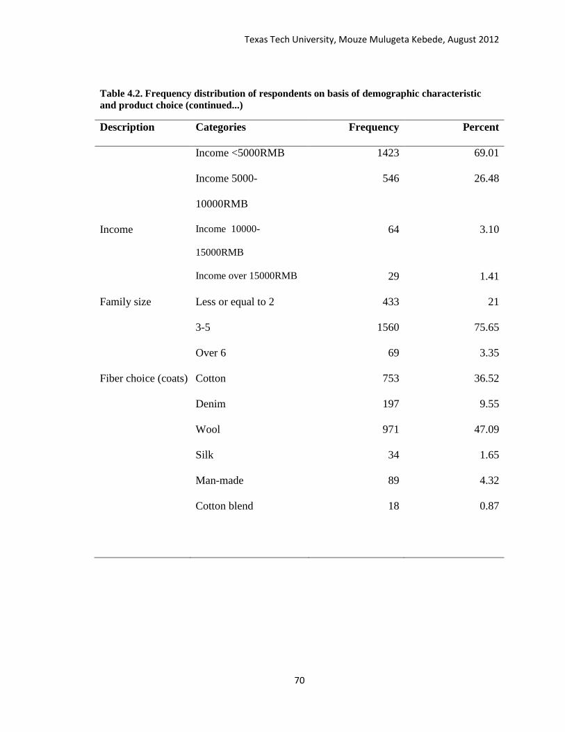
Texas Tech University, Mouze Mulugeta Kebede, August 2012
70
Table 4.2. Frequency distribution of respondents on basis of demographic characteristic
and product choice (continued...)
Description Categories Frequency Percent
Income <5000RMB 1423 69.01
Income 5000-
10000RMB
546 26.48
Income Income 10000-
15000RMB
64 3.10
Income over 15000RMB 29 1.41
Family size Less or equal to 2 433 21
3-5 1560 75.65
Over 6 69 3.35
Fiber choice (coats) Cotton 753 36.52
Denim 197 9.55
Wool 971 47.09
Silk 34 1.65
Man-made 89 4.32
Cotton blend 18 0.87
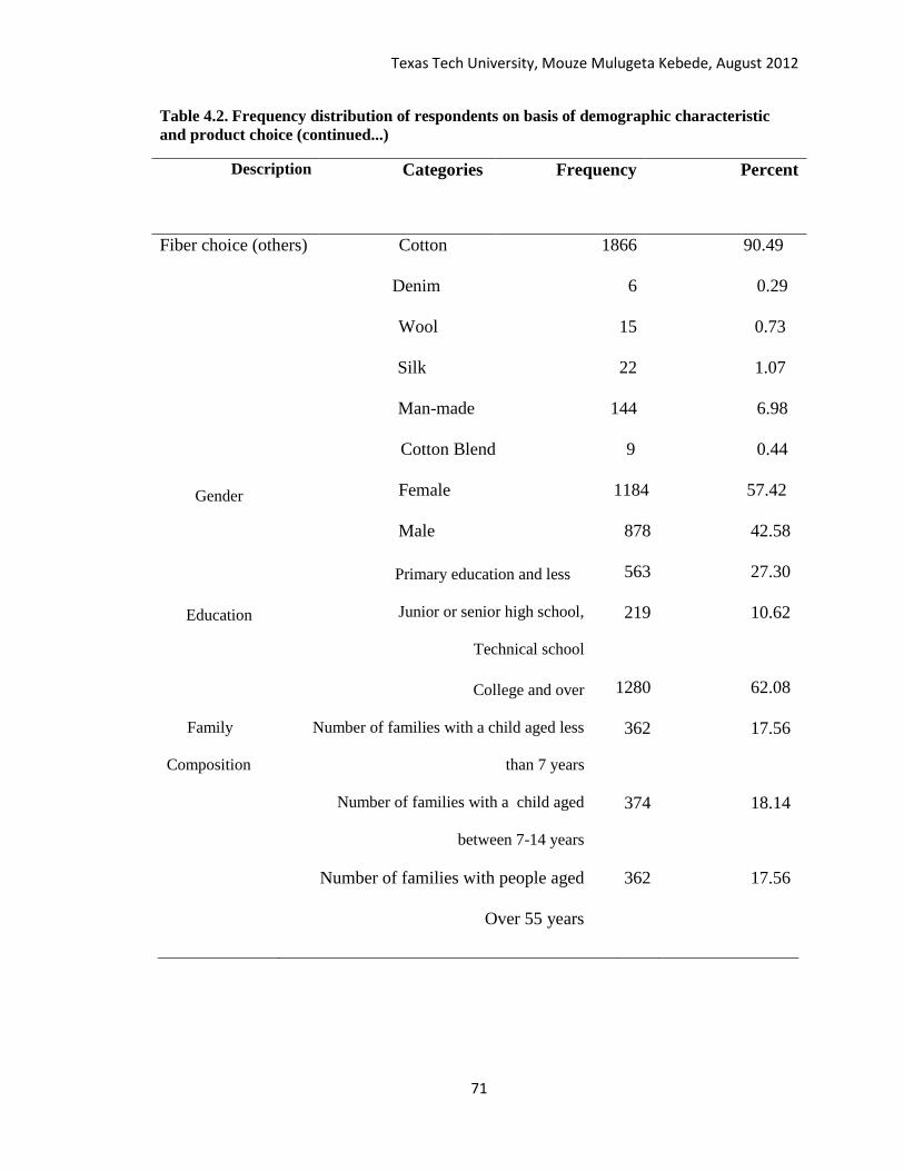
Texas Tech University, Mouze Mulugeta Kebede, August 2012
71
Table 4.2. Frequency distribution of respondents on basis of demographic characteristic
and product choice (continued...)
Description
Categories Frequency Percent
Fiber choice (others) Cotton 1866 90.49
Denim 6 0.29
Wool 15 0.73
Silk 22 1.07
Man-made 144 6.98
Cotton Blend 9 0.44
Gender
Female 1184 57.42
Male 878 42.58
Education
Primary education and less 563 27.30
Junior or senior high school,
Technical school
219 10.62
College and over 1280 62.08
Family
Composition
Number of families with a child aged less
than 7 years
362 17.56
Number of families with a child aged
between 7-14 years
374 18.14
Number of families with people aged
Over 55 years
362 17.56

Texas Tech University, Mouze Mulugeta Kebede, August 2012
72
Summary statistics of quantity, price, and expenditure made on apparel products are
shown under Table 4.3. In general, products under the coats category have the highest
mean price RMB 114.17 per unit, followed by dresses and shirts costing RMB 71.63 and
RMB 50.54, respectively. In regards to the expenditure made by households, respondents,
on average, have made an expenditure equivalent to RMB 249.03 on apparel, with
products under the coat category having the highest expenditure. Taken together, these
findings indicate that the fiber choice of Chinese consumers differ depending on the
products consumed with cotton, man-made, and wool being the preferred fiber choices
for apparel. Products under the “others” category are the least expensive, and, thus, the
most purchased apparel among Chinese households.
Table 4.3. Summary statistics on quantity, price and expenditure
Variable Mean Std Dev
Price
Coat 114.1725 80.6456
Pants 49.5397 35.6002
Shirts 50.5489 35.8787
Dresses 71.6255 36.4273
Others 19.7491 20.7522
Quantity
Coat (consuming households: 54.85% of the sample) 0.8962 1.0880
Pants (consuming households: 53.30% of the sample) 0.8457 1.0602
Shirts (consuming households: 53.54% of the sample) 0.9907 1.2924
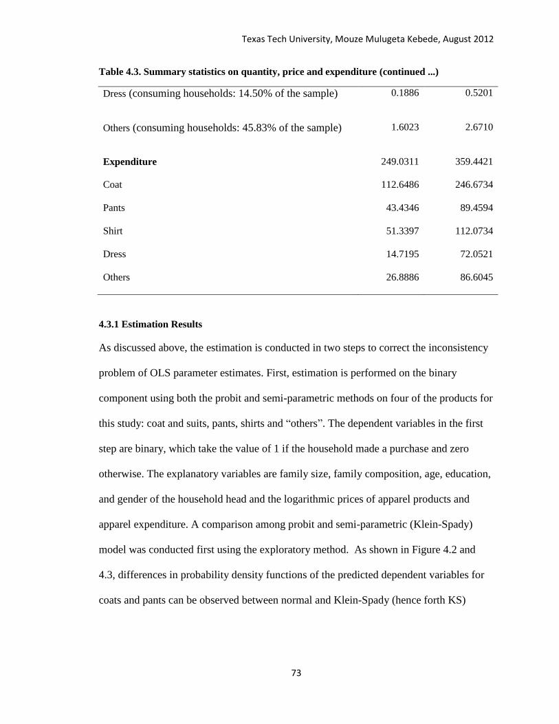
Texas Tech University, Mouze Mulugeta Kebede, August 2012
73
Table 4.3. Summary statistics on quantity, price and expenditure (continued ...)
Dress (consuming households: 14.50% of the sample) 0.1886 0.5201
Others (consuming households: 45.83% of the sample) 1.6023 2.6710
Expenditure 249.0311 359.4421
Coat 112.6486 246.6734
Pants 43.4346 89.4594
Shirt 51.3397 112.0734
Dress 14.7195 72.0521
Others 26.8886 86.6045
4.3.1 Estimation Results
As discussed above, the estimation is conducted in two steps to correct the inconsistency
problem of OLS parameter estimates. First, estimation is performed on the binary
component using both the probit and semi-parametric methods on four of the products for
this study: coat and suits, pants, shirts and “others”. The dependent variables in the first
step are binary, which take the value of 1 if the household made a purchase and zero
otherwise. The explanatory variables are family size, family composition, age, education,
and gender of the household head and the logarithmic prices of apparel products and
apparel expenditure. A comparison among probit and semi-parametric (Klein-Spady)
model was conducted first using the exploratory method. As shown in Figure 4.2 and
4.3, differences in probability density functions of the predicted dependent variables for
coats and pants can be observed between normal and Klein-Spady (hence forth KS)

Texas Tech University, Mouze Mulugeta Kebede, August 2012
74
estimates. Next, the overall correct classification ratio and R-squared12
were calculated to
determine if the semi-parametric (KS) procedure better predicts the binary outcome. The
semi-parametric procedure, as shown in Table 4.4, is able to predict apparel purchases in
all apparel categories better than the probit model. Both correct classification ratio (CCR)
and R2
of KS is higher in all categories indicating a better fit for the KS procedure over
the probit model. In performing CCR procedure, if relates to
and relates to 0, then the prediction is classified as correct. Results
from the second stage estimation also confirm the result found in the first step. Censored
equations based on KS in all the cases have lower mean square error outperforming the
censored equations based on the probit model as shown in Table 4.5.
Figure 4.2. Normal and KS estimate of density function for coats (hn=0.281)
12
As explained by Hayfield and Racine (2008), R2 comparison for parametric and semi-
parametric models can be done using
which is bounded by
[0, 1].
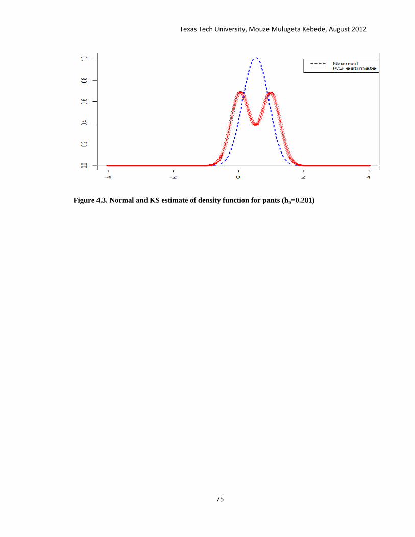
Texas Tech University, Mouze Mulugeta Kebede, August 2012
75
Figure 4.3. Normal and KS estimate of density function for pants (hn=0.281)
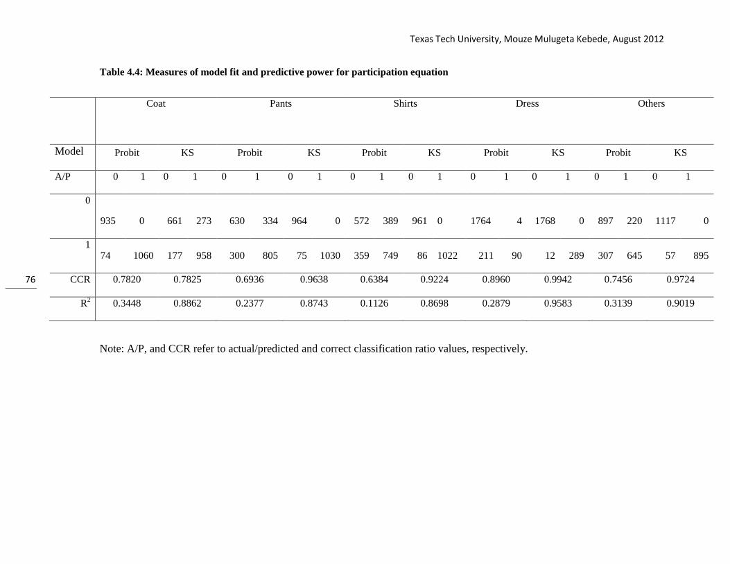
Texas Tech University, Mouze Mulugeta Kebede, August 2012
76
Table 4.4: Measures of model fit and predictive power for participation equation
Note: A/P, and CCR refer to actual/predicted and correct classification ratio values, respectively.
Coat
Pants
Shirts
Dress
Others
Model Probit KS Probit KS Probit KS Probit KS Probit KS
A/P 0 1 0 1 0 1 0 1 0 1 0 1 0 1 0 1 0 1 0 1
0
935 0 661 273 630 334 964 0 572 389 961 0 1764 4 1768 0 897 220 1117 0
1 74 1060 177 958 300 805 75 1030 359 749 86 1022 211 90 12 289 307 645 57 895
CCR 0.7820 0.7825 0.6936 0.9638 0.6384 0.9224 0.8960 0.9942 0.7456 0.9724
R2 0.3448 0.8862 0.2377 0.8743 0.1126 0.8698 0.2879 0.9583 0.3139 0.9019

Texas Tech University, Mouze Mulugeta Kebede, August 2012
77
Table 4.5: Mean square error associated with in sample data
Products
Mean Square Error
Semi-parametric model Probit model
Coats and suits 0.0336 0.1261
Shirts 0.0333 0.1045
Pants 0.0190 0.0678
Others 0.0170 0.0421
Texas Tech University, Mouze Mulugeta Kebede, August 2012
78
Results from the KS procedure and probit model for the coat and pants category are
shown in Table 4.6.13
As per the location and scale restriction, the KS estimator does not
have an intercept and the coefficient for family size was set to 1. The coefficient for
expenditure is positive in the pants equation and is negative in the coats equation under
the KS procedure, but is not significant for both cases. The own-price effect is negative
and significant for both coats and pants equation. Result from KS procedure indicates
that pant price is a significant factor in the household decision to buy coats. The KS
estimate also shows that household heads younger than the ready-to-retire age group, or
who have more than a primary education, or who have a child aged 7-15, or who have an
elderly at home have a higher probability of purchasing coats when compared to the other
household group. In regards to the pant equation, KS procedures indicate that household
heads in the age group of 15-29 are more likely to purchase pants when compared to the
ready-to retire-age group.
13
Results regarding shirts, dress, and “others” equation are reported in Appendix A,
Table 1.
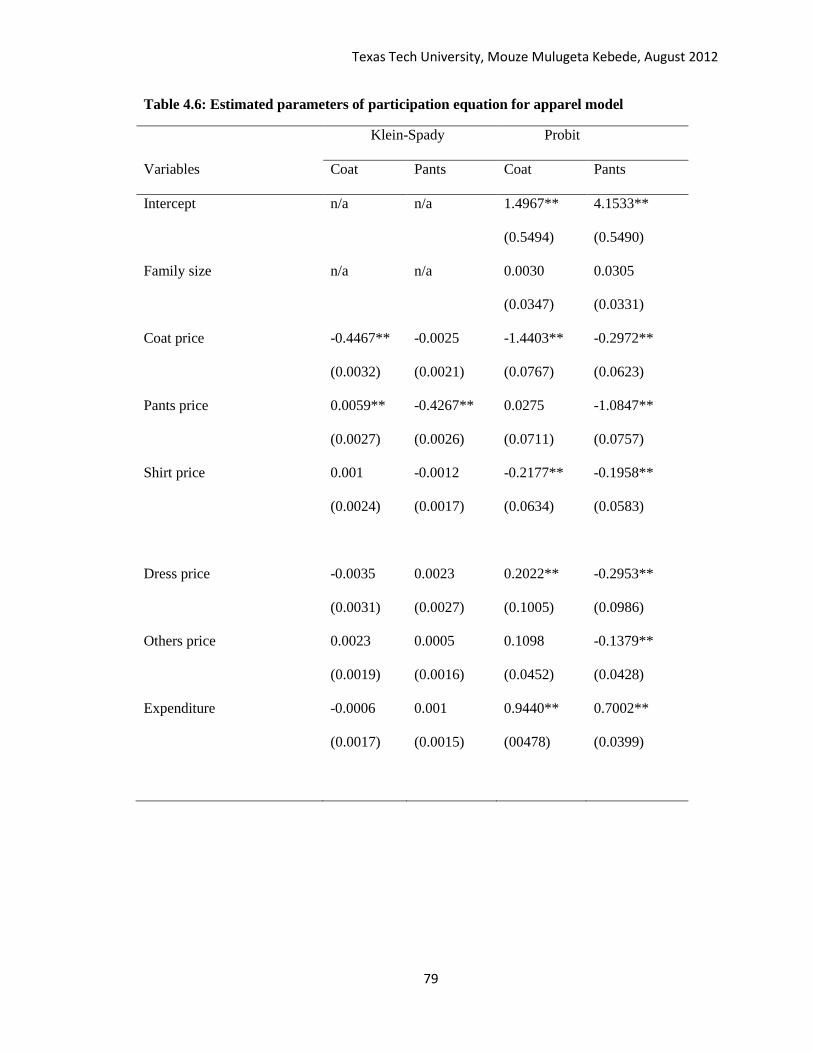
Texas Tech University, Mouze Mulugeta Kebede, August 2012
79
Table 4.6: Estimated parameters of participation equation for apparel model
Klein-Spady Probit
Variables Coat Pants Coat Pants
Intercept n/a n/a 1.4967**
(0.5494)
4.1533**
(0.5490)
Family size n/a n/a 0.0030
(0.0347)
0.0305
(0.0331)
Coat price -0.4467**
(0.0032)
-0.0025
(0.0021)
-1.4403**
(0.0767)
-0.2972**
(0.0623)
Pants price 0.0059**
(0.0027)
-0.4267**
(0.0026)
0.0275
(0.0711)
-1.0847**
(0.0757)
Shirt price 0.001
(0.0024)
-0.0012
(0.0017)
-0.2177**
(0.0634)
-0.1958**
(0.0583)
Dress price
-0.0035
(0.0031)
0.0023
(0.0027)
0.2022**
(0.1005)
-0.2953**
(0.0986)
Others price 0.0023
(0.0019)
0.0005
(0.0016)
0.1098
(0.0452)
-0.1379**
(0.0428)
Expenditure -0.0006
(0.0017)
0.001
(0.0015)
0.9440**
(00478)
0.7002**
(0.0399)
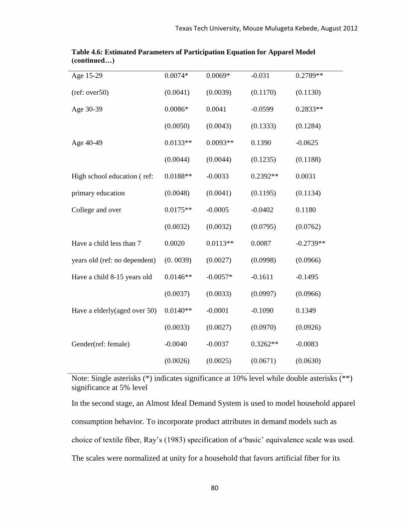
Texas Tech University, Mouze Mulugeta Kebede, August 2012
80
Table 4.6: Estimated Parameters of Participation Equation for Apparel Model
(continued…)
Age 15-29
(ref: over50)
0.0074*
(0.0041)
0.0069*
(0.0039)
-0.031
(0.1170)
0.2789**
(0.1130)
Age 30-39 0.0086* 0.0041 -0.0599 0.2833**
(0.0050) (0.0043) (0.1333) (0.1284)
Age 40-49 0.0133**
(0.0044)
0.0093**
(0.0044)
0.1390
(0.1235)
-0.0625
(0.1188)
High school education ( ref:
primary education
0.0188**
(0.0048)
-0.0033
(0.0041)
0.2392**
(0.1195)
0.0031
(0.1134)
College and over 0.0175**
(0.0032)
-0.0005
(0.0032)
-0.0402
(0.0795)
0.1180
(0.0762)
Have a child less than 7
years old (ref: no dependent)
0.0020
(0. 0039)
0.0113**
(0.0027)
0.0087
(0.0998)
-0.2739**
(0.0966)
Have a child 8-15 years old 0.0146**
(0.0037)
-0.0057*
(0.0033)
-0.1611
(0.0997)
-0.1495
(0.0966)
Have a elderly(aged over 50) 0.0140**
(0.0033)
-0.0001
(0.0027)
-0.1090
(0.0970)
0.1349
(0.0926)
Gender(ref: female) -0.0040 -0.0037 0.3262** -0.0083
(0.0026) (0.0025) (0.0671) (0.0630)
Note: Single asterisks (*) indicates significance at 10% level while double asterisks (**)
significance at 5% level
In the second stage, an Almost Ideal Demand System is used to model household apparel
consumption behavior. To incorporate product attributes in demand models such as
choice of textile fiber, Ray’s (1983) specification of a‘basic’ equivalence scale was used.
The scales were normalized at unity for a household that favors artificial fiber for its
Texas Tech University, Mouze Mulugeta Kebede, August 2012
81
apparel. Starting from a household expenditure function that represents a household who
favors artificial fiber for its apparel, a given household expenditure can be specified as:
4.18
where is the cost function for the reference household, is a general
equivalence scale formulated as where and are fiber
choice by households and their coefficients, respectively. Then
will be
a cost index for fiber type in relation to artificial fibers. Furthermore, the analysis uses the
translation approach proposed by Pollak and Wales to incorporate demographic variables
into the AIDS system. That is, the intercept in the budget share equation is augmented by
where is the value of the demographic variable. Theoretical
restrictions of homogeneity and symmetry were maintained during estimation, but the
theoretical restriction of adding up on parameter estimates, in general, does not hold as in
the conventional case as discussed by Yen, Kan, and Jiuan Su. As a result, estimation on
the budget equation was made by treating the dress category as a residual good as
suggested by Yen, Lin, and Smallwood and estimating n-1 equations with an
identity . To ensure our elasticity estimates are in line with economic
theory, this study used, as suggested by Yen, Kan, and Jiuan Su, Euler aggregation
(
14to recover cross price effects of dress goods group on coats, pants,
shirts and “others” categories. Engle aggregation was also used to
recover the income elasticity of the dress group. Cournot aggregation
was used to calculate the elasticity of dress group demand to coat, pants,
14
Here refer to cross price elasticity, budget share and income elasticity of a
given product, respectively.
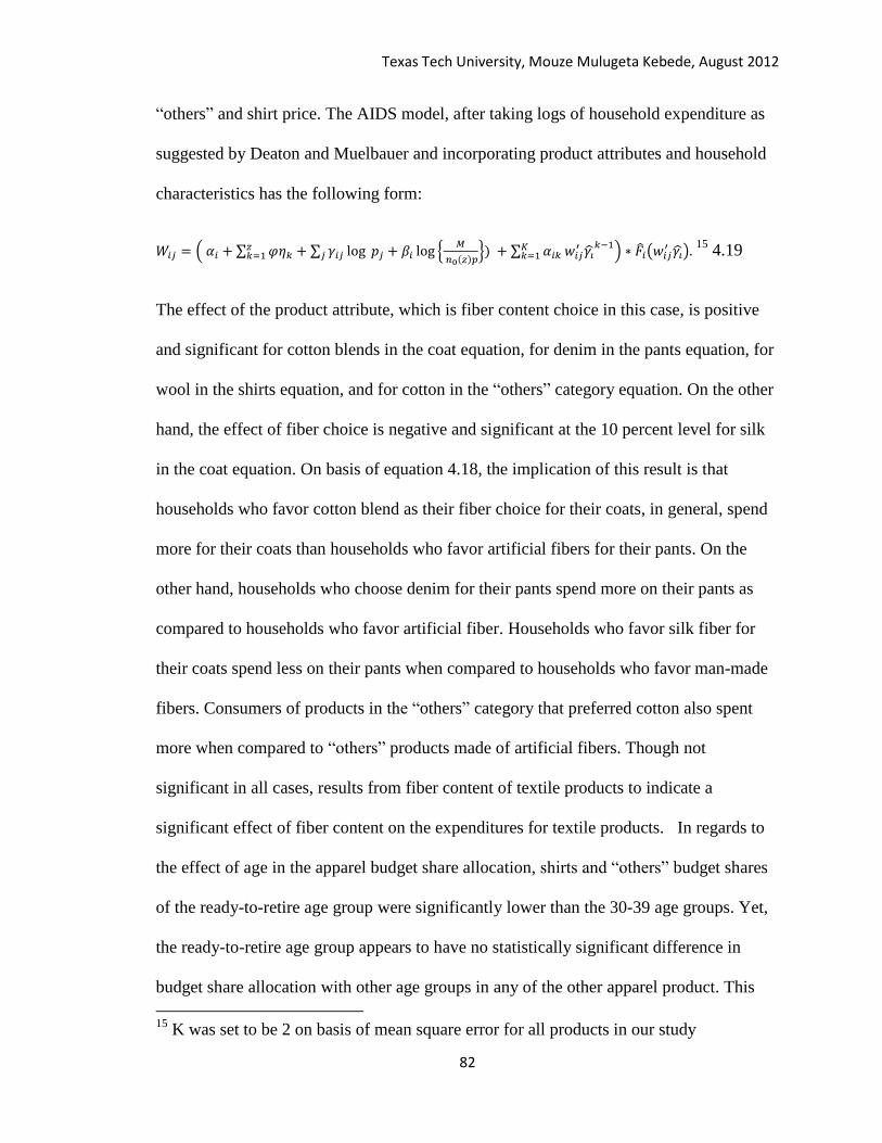
Texas Tech University, Mouze Mulugeta Kebede, August 2012
82
“others” and shirt price. The AIDS model, after taking logs of household expenditure as
suggested by Deaton and Muelbauer and incorporating product attributes and household
characteristics has the following form:
15
4.19
The effect of the product attribute, which is fiber content choice in this case, is positive
and significant for cotton blends in the coat equation, for denim in the pants equation, for
wool in the shirts equation, and for cotton in the “others” category equation. On the other
hand, the effect of fiber choice is negative and significant at the 10 percent level for silk
in the coat equation. On basis of equation 4.18, the implication of this result is that
households who favor cotton blend as their fiber choice for their coats, in general, spend
more for their coats than households who favor artificial fibers for their pants. On the
other hand, households who choose denim for their pants spend more on their pants as
compared to households who favor artificial fiber. Households who favor silk fiber for
their coats spend less on their pants when compared to households who favor man-made
fibers. Consumers of products in the “others” category that preferred cotton also spent
more when compared to “others” products made of artificial fibers. Though not
significant in all cases, results from fiber content of textile products to indicate a
significant effect of fiber content on the expenditures for textile products. In regards to
the effect of age in the apparel budget share allocation, shirts and “others” budget shares
of the ready-to-retire age group were significantly lower than the 30-39 age groups. Yet,
the ready-to-retire age group appears to have no statistically significant difference in
budget share allocation with other age groups in any of the other apparel product. This
15
K was set to be 2 on basis of mean square error for all products in our study

Texas Tech University, Mouze Mulugeta Kebede, August 2012
83
result augments the resulted reported for the aggregate case. Based on the previous
chapter, the ready-to-retire age group had lower expense in apparel when compared to
households in the age group of 30-39. According to results reported here, much of the
decline in apparel spending is a result of their lower expense on shirts and “others” group.
Table 4.7: Estimated parameters of apparel AIDS model
Budget share equation parameters Coats Pants Shirts Others
Intercept 0.1831** 0.2252** 0.1020* 0.0688
(0.0454) (0.0507) (0.0562) (0.0507)
Age 15-29 reference (over 54) -0.0153 -0.0082 0.0447 0.0205
(0.0273) (0.0250) (0.0282) (0.0206)
Age 30-39 -0.0093 -0.0168 0.0744** 0.0483**
(0.0309) (0.0282) (0.0314) (0.0231)
Age 40-49 -0.0048 -0.0495* 0.0417 0.0315
(0.0289) (0.0270) (0.0300) (0.0217)
High school education ( ref: primary education -0.0117 -0.0528** -0.1128** -0.0592**
(0.0282) (0.0264) (0.0297) (0.0229)
College and over -0.0264 -0.0429** -0.0575** -0.0414**
(0.0184) (0.0166) (0.0185) (0.0139)
Have a child aged < 7(ref: no dependent) -0.0305 0.0175 0.0130 -0.0122
(0.0220) (0.0193) (0.0215) (0.0166)
Have a child aged b/n 7-15 -0.0227 0.0077 -0.0279 -0.0141
(0.0238) (0.0213) (0.0230) (0.0178)
Have a elderly at home aged>54 -0.0299 -0.0538** -0.0650** -0.0511**
(0.0219) (0.0189) (0.0216) (0.0162)
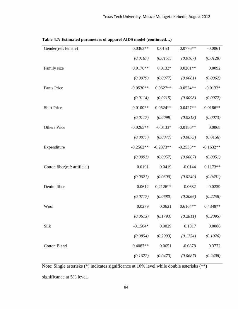
Texas Tech University, Mouze Mulugeta Kebede, August 2012
84
Table 4.7: Estimated parameters of apparel AIDS model (continued…)
Gender(ref: female) 0.0363** 0.0153 0.0776** -0.0061
(0.0167) (0.0151) (0.0167) (0.0128)
Family size 0.0176** 0.0132* 0.0201** 0.0092
(0.0079) (0.0077) (0.0081) (0.0062)
Pants Price -0.0530** 0.0627** -0.0524** -0.0133*
(0.0114) (0.0215) (0.0098) (0.0077)
Shirt Price -0.0100** -0.0524** 0.0427** -0.0186**
(0.0117) (0.0098) (0.0218) (0.0073)
Others Price -0.0265** -0.0133* -0.0186** 0.0068
(0.0077) (0.0077) (0.0073) (0.0156)
Expenditure -0.2562** -0.2373** -0.2535** -0.1632**
(0.0091) (0.0057) (0.0067) (0.0051)
Cotton fiber(ref: artificial) 0.0191 0.0419 -0.0144 0.1173**
(0.0621) (0.0300) (0.0240) (0.0491)
Denim fiber 0.0612 0.2126** -0.0632 -0.0239
(0.0717) (0.0680) (0.2066) (0.2258)
Wool 0.0279 0.0621 0.6164** 0.4348**
(0.0613) (0.1793) (0.2811) (0.2095)
Silk -0.1504* 0.0829 0.1817 0.0086
(0.0854) (0.2993) (0.1734) (0.1076)
Cotton Blend 0.4087** 0.0651 -0.0878 0.3772
(0.1672) (0.0473) (0.0687) (0.2408)
Note: Single asterisks (*) indicates significance at 10% level while double asterisks (**)
significance at 5% level.

Texas Tech University, Mouze Mulugeta Kebede, August 2012
85
Households with primary education appear to allocate more for pants, shirts, and
“others” when compared to households with high school or college education. Family
composition, such as the presence of a child or elderly, did not have statistically
significant effects on budget allocation for the coat category. But, in line with results
from Lee et al., and Wagner, the presence of an elderly (aged over 50) in a household had
a significant and inverse impact on pants, shirts, and “others” budget allocation. Men
headed households had a significantly higher budget share for coats and shirts than their
female counterpart. The effect of family size on apparel expenditure share is significant
and positive for all apparel products.
Marshallian elastcities were calculated on conditional budget shares using the approach
employed by Sam and Zheng. Accordingly, the uncompensated own-price elasticities for
all apparel products are significant and negative. This indicates that apparel products
have a downward slopping demand curve as expected. Furthermore, own-price elasticity
estimates suggest that “others” consumption is more sensitive to own-price changes as it
has the highest own price elasticity value when compared to other apparel products.
Expenditure elastcities are positive and significant for all apparel products. Products
under the dress category have the highest expenditure elasticity indicating they are the
most responsive to changes in apparel spending by consumers. The cross-price elasticity
of coats is significant and positive with pants and shirts indicating gross substitutes. In
particular, a one percent decline in coat price will cause 5% decline in pants and 12%
percent decline in expenditure for shirts products. On the other hand, a one percent
increase in price for pants is likely to cause a 0. 4 % increase in coats consumption, while
a one percent increase in price for shirts will cause an increase in coats consumption by
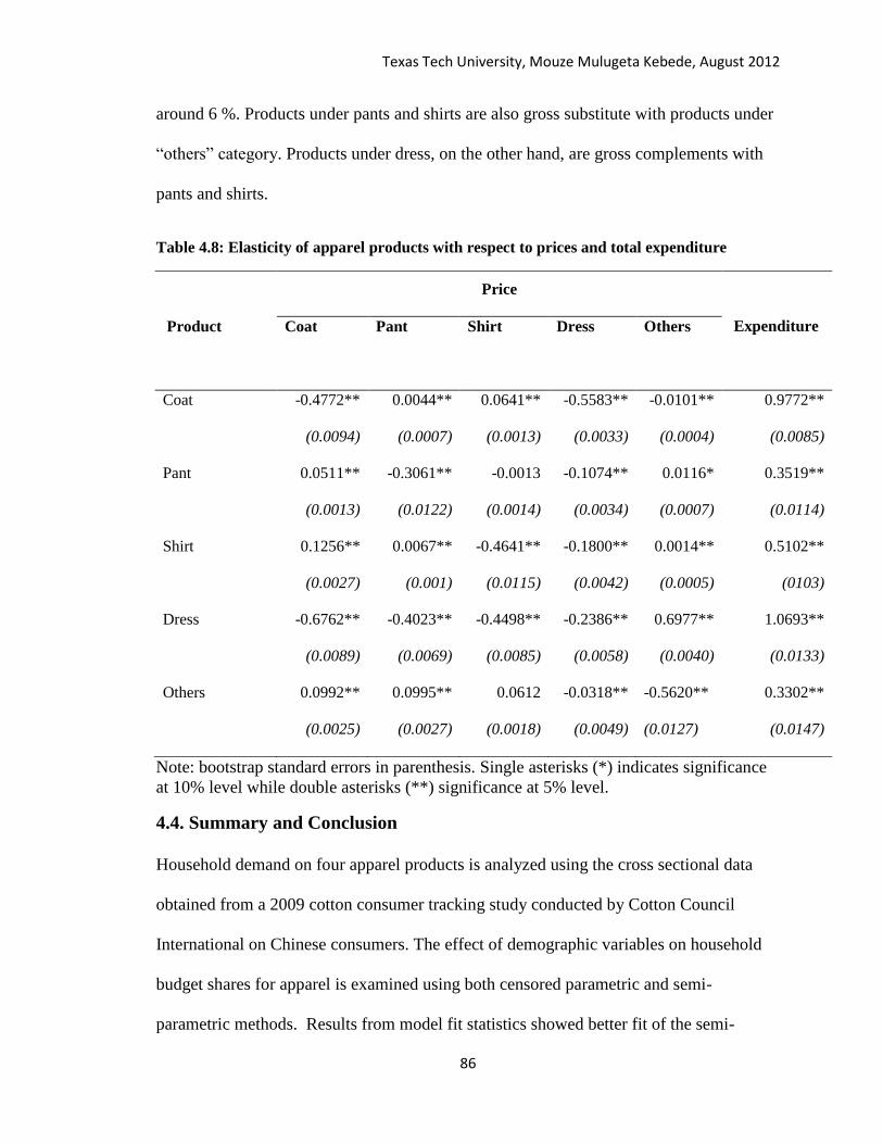
Texas Tech University, Mouze Mulugeta Kebede, August 2012
86
around 6 %. Products under pants and shirts are also gross substitute with products under
“others” category. Products under dress, on the other hand, are gross complements with
pants and shirts.
Table 4.8: Elasticity of apparel products with respect to prices and total expenditure
Product
Price
Expenditure
Coat
Pant
Shirt
Dress
Others
Coat
-0.4772**
(0.0094)
0.0044**
(0.0007)
0.0641**
(0.0013)
-0.5583**
(0.0033)
-0.0101**
(0.0004)
0.9772**
(0.0085)
Pant
0.0511**
(0.0013)
-0.3061**
(0.0122)
-0.0013
(0.0014)
-0.1074**
(0.0034)
0.0116*
(0.0007)
0.3519**
(0.0114)
Shirt
0.1256**
(0.0027)
0.0067**
(0.001)
-0.4641**
(0.0115)
-0.1800**
(0.0042)
0.0014**
(0.0005)
0.5102**
(0103)
Dress
-0.6762**
(0.0089)
-0.4023**
(0.0069)
-0.4498**
(0.0085)
-0.2386**
(0.0058)
0.6977**
(0.0040)
1.0693**
(0.0133)
Others
0.0992**
(0.0025)
0.0995**
(0.0027)
0.0612
(0.0018)
-0.0318**
(0.0049)
-0.5620**
(0.0127)
0.3302**
(0.0147)
Note: bootstrap standard errors in parenthesis. Single asterisks (*) indicates significance
at 10% level while double asterisks (**) significance at 5% level.
4.4. Summary and Conclusion
Household demand on four apparel products is analyzed using the cross sectional data
obtained from a 2009 cotton consumer tracking study conducted by Cotton Council
International on Chinese consumers. The effect of demographic variables on household
budget shares for apparel is examined using both censored parametric and semi-
parametric methods. Results from model fit statistics showed better fit of the semi-
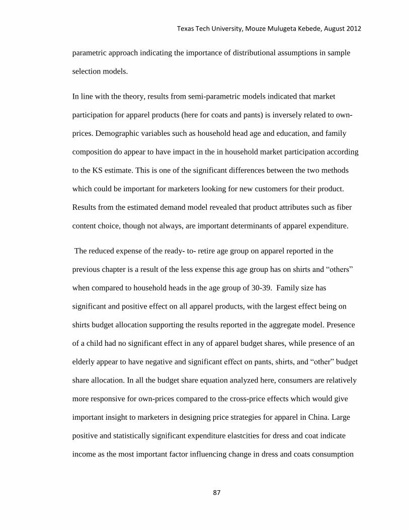
Texas Tech University, Mouze Mulugeta Kebede, August 2012
87
parametric approach indicating the importance of distributional assumptions in sample
selection models.
In line with the theory, results from semi-parametric models indicated that market
participation for apparel products (here for coats and pants) is inversely related to own-
prices. Demographic variables such as household head age and education, and family
composition do appear to have impact in the in household market participation according
to the KS estimate. This is one of the significant differences between the two methods
which could be important for marketers looking for new customers for their product.
Results from the estimated demand model revealed that product attributes such as fiber
content choice, though not always, are important determinants of apparel expenditure.
The reduced expense of the ready- to- retire age group on apparel reported in the
previous chapter is a result of the less expense this age group has on shirts and “others”
when compared to household heads in the age group of 30-39. Family size has
significant and positive effect on all apparel products, with the largest effect being on
shirts budget allocation supporting the results reported in the aggregate model. Presence
of a child had no significant effect in any of apparel budget shares, while presence of an
elderly appear to have negative and significant effect on pants, shirts, and “other” budget
share allocation. In all the budget share equation analyzed here, consumers are relatively
more responsive for own-prices compared to the cross-price effects which would give
important insight to marketers in designing price strategies for apparel in China. Large
positive and statistically significant expenditure elastcities for dress and coat indicate
income as the most important factor influencing change in dress and coats consumption

Texas Tech University, Mouze Mulugeta Kebede, August 2012
88
pattern. Given the prevailing price structure, expenditure on dress and coats will increase
with increases in household income.

Texas Tech University, Mouze Mulugeta Kebede, August 2012
89
Chapter Five
Implications of Changes in Chinese Demographic Structure on World
Cotton Market
Introduction
China is one of the leading cotton fiber consumers accounting for over39 percent of world
consumption in aggregate terms in 2008 (ICAC). Moreover, per capita domestic consumption of
textile fiber grew at a rate of 7.15% per annum between 2000-2008. By comparison, however,
total consumption figures are still far below the developed world consumption level on per capita
basis, as shown in Figure 5.1. Given the relatively higher Chinese budget share for clothing ($5.8
for every $ 100) compared to the developed world such as the U.S ($3.5 for every $100) and the
rapid increase in the Chinese household income observed in recent years, domestic demand for
textiles is expected to grow rapidly. According to the National Bureau of Statistics (NBS), per
capita textile expenditure of urban households has increased, on average, by 12.5% to 1444.34
Yuan in 2010, while cash expenditure on textiles of the lowest income rural households increased
to 150.84 Yuan, up by 11.9% from its 2009 value. Such a rapid growth rate, according to some
analysts, is expected to make China one of the largest markets for textiles by 2020, making it
20% larger than the Japan market (Kurt Salmon Associates as cited in Zhang et al.). However,
China is also experiencing dramatic changes in its demographic structure since launching of its
population policy in 1979, which has ramifications that could threaten the path of the per capita
income rate growth. Notable changes in demographic structure, according to Gao and Zhai,
include increases in urban population (to over 45 percent of the total population), increases in
proportion of educated people (8.9 %), increases in the proportion of elderly people (8.16 percent
in 2002), and a decline in the household size (3.1 people per household).
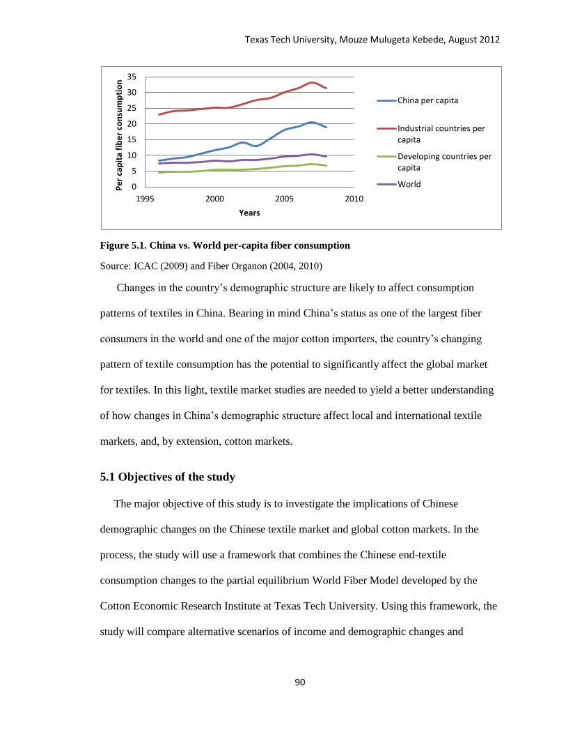
Texas Tech University, Mouze Mulugeta Kebede, August 2012
90
Figure 5.1. China vs. World per-capita fiber consumption
Source: ICAC (2009) and Fiber Organon (2004, 2010)
Changes in the country’s demographic structure are likely to affect consumption
patterns of textiles in China. Bearing in mind China’s status as one of the largest fiber
consumers in the world and one of the major cotton importers, the country’s changing
pattern of textile consumption has the potential to significantly affect the global market
for textiles. In this light, textile market studies are needed to yield a better understanding
of how changes in China’s demographic structure affect local and international textile
markets, and, by extension, cotton markets.
5.1 Objectives of the study
The major objective of this study is to investigate the implications of Chinese
demographic changes on the Chinese textile market and global cotton markets. In the
process, the study will use a framework that combines the Chinese end-textile
consumption changes to the partial equilibrium World Fiber Model developed by the
Cotton Economic Research Institute at Texas Tech University. Using this framework, the
study will compare alternative scenarios of income and demographic changes and
0
5
10
15
20
25
30
35
1995 2000 2005 2010
Pe
r ca
pit
a fi
be
r co
nsu
mp
tio
n
Years
China per capita
Industrial countries per capita
Developing countries per capita
World
Texas Tech University, Mouze Mulugeta Kebede, August 2012
91
examine their effect on textile and cotton markets. The study will specifically analyze
two sets of scenarios:
First, the impact of growth in Chinese per capita income on global cotton and
textile trade markets is examined. Domestic demand is expected to grow in
tandem with increases in per capita income; conversely the cost of textile
production, through wage rate increases (per capita income increases), is likely to
be higher for textile firms, thereby increasing textile prices and reducing per
capita fiber consumption.
Second, the impact of an increase in the proportion of Chinese elderly population
and decline in family size on global textile and fiber markets is analyzed. Changes
in these variables, in general, will likely have an inward shift of Chinese textile
demand which would, in turn, inversely affect global demand for fiber.
5.2 Conceptual Framework
Changes in demand and supply factors have implications beyond the immediate
market. Just, Hueth and Schmitz developed a model that can be used for analyzing
interlinked markets that overcomes some of the weakness of analyzing single markets
while requiring less data than general equilibrium models. This research, in turn, has
motivated a number of empirical studies in policy analysis. Notable works within the
textile markets literature include studies by Hudson and Ethridge and Sumner. Given the
use of such an approach to analyze policy changes across markets, a theoretical
framework on the basis of such existing works was developed.
Texas Tech University, Mouze Mulugeta Kebede, August 2012
92
The model used in this analysis is based on a partial equilibrium framework and
static16
world trade models. In Figure 5.2, the eight panels show the price-quantity
relationship for homogeneous cotton and end-use textile products based on supply-
demand interactions. Two commodities are assumed: raw cotton and end-use textile
products, and three regions of the world: U.S., China, and a small textile exporting-cotton
importing country. In figures 5.2a, b, c and d, the lines Si and Di represent domestic
supply and demand curves for end-use textiles in each of the three countries. Assuming a
closed economy, price-quantity equilibrium is shown by Pd0 and Q0 for each of the three
countries in the analysis. On the other hand, panel 5.2e, f, g and h, the lines Si and Di
represent domestic supply and demand curves for cotton in each of the respective
countries.
Assuming ceteris paribus, Figure 5.2 describes how changes in Chinese per capita
income, size of elderly population and family size affect the world textile and cotton
markets. An increase in per capita income in China shifts the demand for textiles
outward to D1 and, at the same time, shifts domestic production of textiles inward to S1
due increases in labor cost. That is, an increase in per capita income is likely to raise
textile production cost, thus moving inward the textile supply curve. Free trade among
each of these countries moves world price for textiles to PW0. With increase in Chinese
per capita income, world textile price rises or falls depending on the relative elasticity of
the Chinese supply and demand curves and the magnitude of the shifts. Here, world price
for textiles is expected to rise to PW1. The initial equilibrium for world textile markets is
shown by excess supply curve (ES0) and excess demand curve (ED0). The quantity traded
16
Refers to analysis on relationships between variables with the same time period.
Texas Tech University, Mouze Mulugeta Kebede, August 2012
93
for textiles as a result of income changes is expected to be at (QT1) as excess supply
moves inward from ES0 to ES1. In regards to the cotton market, the effects of increases in
per capita income on Chinese domestic mill consumption is likely to be inverse, thus
moving domestic consumption of cotton from QSC0 to QSC1. This occurs as a result of a
decline in the domestic textile production, which as discussed above occurs owing to
increase in the labor cost. This move, in turn, would put downward pressure on world
cotton price moving it from PWC0 to PWC1. U.S. exports of cotton would, as a result,
decline from QSC0 to QSC1. In this scenario, however, the small country competing in
the textile export market and importing cotton is anticipated to increase its exports of
textiles from (QS0 to QS1) and imports of cotton from (QSC0-QDC0) to (QSC1-QDC1).
An inclusion of the elderly proportion and family size effect would have the following
impacts: domestic demand for textiles would shrink to D2, which would lower world
textile price and move it to PW2; Traded textiles on world markets would increase as a
result of lower world textile price; the Chinese cotton demand is expected to shift further
inward to QSC2 and, thus, the world price for cotton as demand for cotton declines in
China; Quantity traded of cotton increases from QTC1 to QTC2. Additionally, U.S
exports of cotton would also decline as a result of a decline in world price for cotton. In
regards to the small trading country, exports for textiles would decline while cotton
imports would be expected to increase as a result of the lower world price for cotton.

Texas Tech University, Mouze Mulugeta Kebede , August 2012
94
Figure 5.2. Effects of Chinese demographic and economic changes on World textile and cotton market

Texas Tech University, Mouze Mulugeta Kebede, August 2012
95
5.3 Data Source and Description
Raw data from a cotton consumer tracking study conducted by Cotton Council
International is used to estimate the effects of income and demographic variables on
Chinese textile consumption. In total, a survey response from 6539 households in 24
cities is used for this analysis. The estimates of household textile demand presented in
Chapter Three, Table 3.6 and 3.7, are used as a basis for the estimation. Time series data
used for this study are compiled from different sources: annual data on the Chinese
textile index, Chinese population size, Chinese old age proportion, Chinese family size
and per capita income is obtained from National Bureau of Statistics of China (NBS);
cotton prices, production, consumption, stocks, and trade is taken from the USDA
(Production, Supply, and Distribution Database); and fiber mill consumption, and man-
made fiber data are obtained from the Food and Agricultural Organization (FAO), World
Fiber Consumption Survey and Fiber Organon. Data on the world textile price index is
taken from International Cotton Advisory Committee (ICAC), while macroeconomic data
such as CPI, exchange rate, and oil prices are collected from Food and Agricultural
Policy Research Institute (FAPRI).
5.4 Methods and Procedures
The econometric model developed here will mainly address the demand side of the
Chinese textile market and incorporate the results from the Chinese demand model to the
World Fiber Model developed by the Cotton Economics Research Institute at Texas Tech
University. The model is described in detail in Pan et al. (2004) and includes 35 major
cotton exporting and importing countries of the world. The model incorporates
productivity differences within some regions of the world, fiber substitutability and

Texas Tech University, Mouze Mulugeta Kebede, August 2012
96
linkages between upstream (apparel industry) and downstream (cotton production)
production sectors within these regions.
Textile Supply and Demand
The Chinese cotton-textile market is modeled with three types of agents as major
players in the markets: cotton producers, textile producers and final consumers. These
agents interact in two vertically integrated markets. The first of these markets is the
textile sector market, which is composed of domestic textile demand, textile trade, and
cotton mill use or textile production components. These three components are joined by
the identity:
textileqi +Imtt= Dctt+Extt 5.1
where textileqi is domestic production and Imtt is import demand, both representing the
supply side, and Dctt is domestic consumption and Extt is export supply for textiles, both
representing the supply side.
Domestic textile production is modeled as a function Chinese textile price index
( ), Chinese per capita income ( ) as a proxy for wage rate, and Chinese
domestic cotton price ( :
The other element in the textile supply equation is the net export supply function.
The net export supply function (NEXTt) is specified as function of the Chinese textile
price index ( ), world textile price index (Pitwt) and price of petroleum (PPt) as a
measure of transportation cost and lagged textile net exports (Lnextt).

Texas Tech University, Mouze Mulugeta Kebede, August 2012
97
5.3
After identifying the textile supply function, the next step is estimation of demand
functions for textiles. In estimating demand for textile products (apparel, home-textiles,
and others), the results of the AIDS model presented in chapter Three under Table 3.7
and 3.9 are used.
Cotton Supply and Demand
Results from the textile sector model are incorporated into the partial equilibrium
World Fiber Model developed by the Cotton Economics Research Institute at Texas Tech
University. In this framework, each country is modeled as an individual buyer and seller
in the global market. On the demand side, because cotton is an input in the production of
textiles, its demand is derived from the demand for textiles. Domestic textile fiber
consumption is computed using the conventional approach used by USDA (US
Department of Agriculture) and ICAC (International Cotton Advisory Committee). It is
calculated as the difference between fiber spun by Chinese mills and the amount of fiber
contained in Chinese net-exports. On the supply side, cotton production is defined from
structural equations of yield and area allocation. Section 2.3 provides a detail description
of the global fiber model (or sees Pan et al. for further discussion of the model).
5.5 Results and Discussions Income and textile expenditure relationships are presented in Table 5.1. The income
elasticity of textile expenditure shows that textile consumption would increase by 0.59
percent with 1 percent increase in income. Estimates of household textile consumption,
on basis of AIDS model, are indicated in Table 3.7 and 3.9. The expenditure elasticities
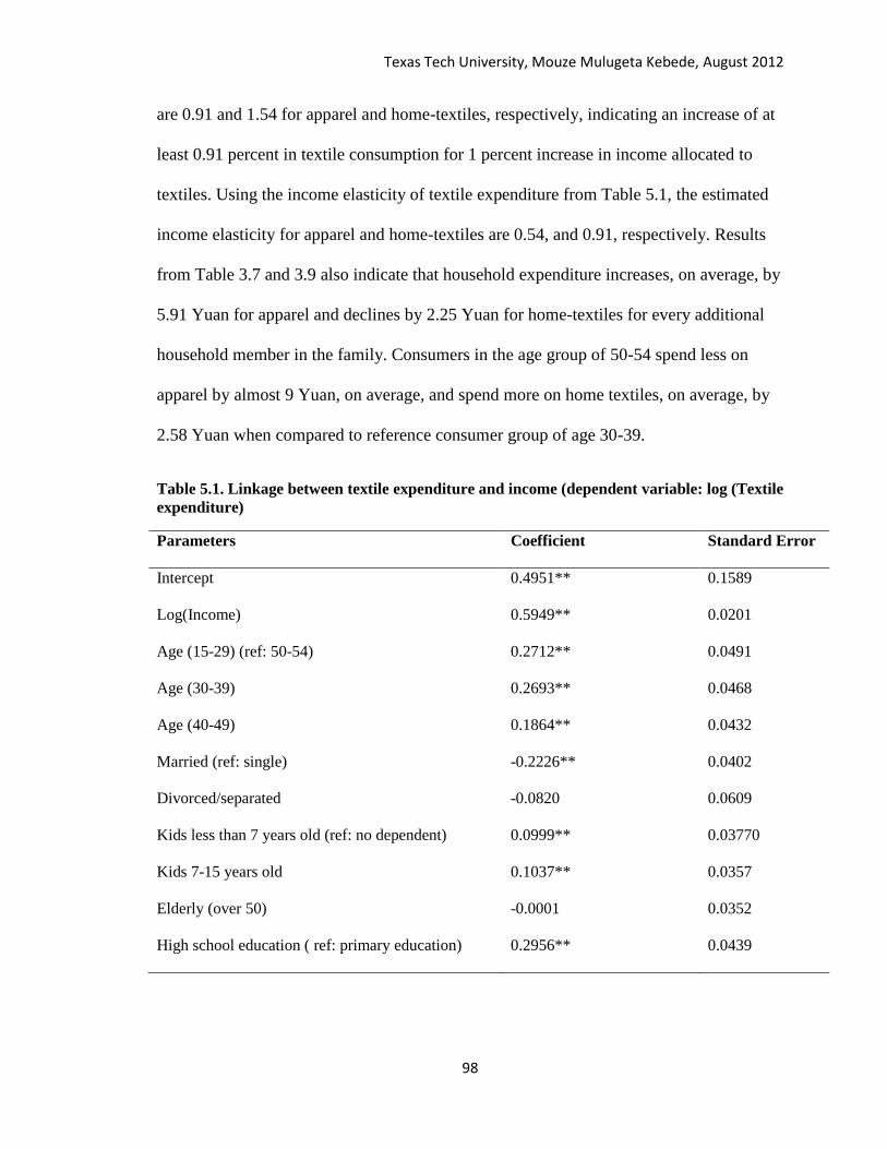
Texas Tech University, Mouze Mulugeta Kebede, August 2012
98
are 0.91 and 1.54 for apparel and home-textiles, respectively, indicating an increase of at
least 0.91 percent in textile consumption for 1 percent increase in income allocated to
textiles. Using the income elasticity of textile expenditure from Table 5.1, the estimated
income elasticity for apparel and home-textiles are 0.54, and 0.91, respectively. Results
from Table 3.7 and 3.9 also indicate that household expenditure increases, on average, by
5.91 Yuan for apparel and declines by 2.25 Yuan for home-textiles for every additional
household member in the family. Consumers in the age group of 50-54 spend less on
apparel by almost 9 Yuan, on average, and spend more on home textiles, on average, by
2.58 Yuan when compared to reference consumer group of age 30-39.
Table 5.1. Linkage between textile expenditure and income (dependent variable: log (Textile
expenditure)
Parameters Coefficient Standard Error
Intercept 0.4951** 0.1589
Log(Income) 0.5949** 0.0201
Age (15-29) (ref: 50-54) 0.2712** 0.0491
Age (30-39) 0.2693** 0.0468
Age (40-49) 0.1864** 0.0432
Married (ref: single) -0.2226** 0.0402
Divorced/separated -0.0820 0.0609
Kids less than 7 years old (ref: no dependent) 0.0999** 0.03770
Kids 7-15 years old 0.1037** 0.0357
Elderly (over 50) -0.0001 0.0352
High school education ( ref: primary education) 0.2956** 0.0439

Texas Tech University, Mouze Mulugeta Kebede, August 2012
99
Table 5.1. Linkage between textile expenditure and income (dependent variable: log(Textile
expenditure) continued.....
College and over 0.2791** 0.0288
Gender(ref: women) -0.3664** 0.0238
Family size -0.0497** 0.0126
East region(ref: north) -0.059* 0.0327
Central region -0.3558** 0.0359
South region -0.3101** 0.0378
South-west region 0.0089 0.0365
R2 0.23
** significant at 5% level and * significant at 10% level.
Estimates on Cotton Textile Trade and Production
Estimates in regards to Chinese textile production and trade are presented in Table 5.2.
Parameter estimates for textile production indicate that changes in cotton prices and the
wage rate have negative impacts on textile production, while the textile price index has
positive and statistically significant effect on textile production. Among explanatory
variables, changes in cotton prices affects textile production more when compared to the
wage rate and the price for textiles, indicating more sensitivity of the industry to input
than output prices. Chinese textile net exports, on the other hand, are most influenced by
the domestic textile price index as for every 1 percent increase in domestic prices, net
exports decline by over 1 percent.
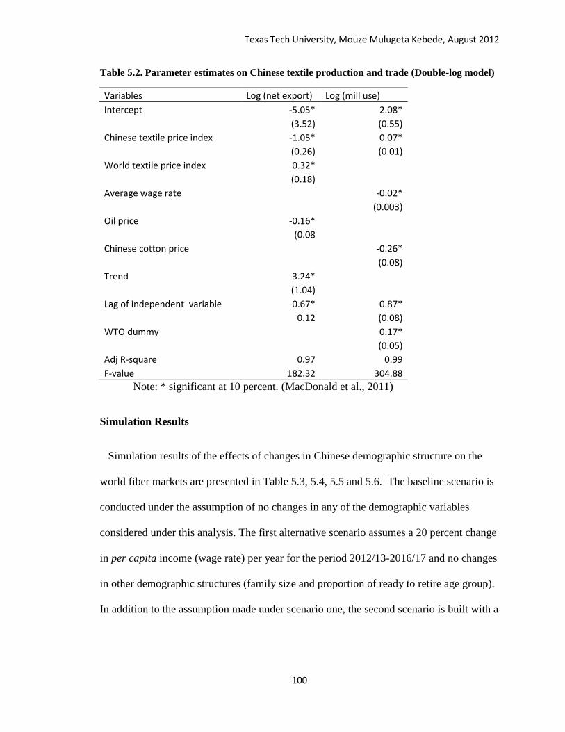
Texas Tech University, Mouze Mulugeta Kebede, August 2012
100
Table 5.2. Parameter estimates on Chinese textile production and trade (Double-log model)
Variables Log (net export) Log (mill use)
Intercept -5.05* 2.08*
(3.52) (0.55)
Chinese textile price index -1.05* 0.07*
(0.26) (0.01)
World textile price index 0.32*
(0.18)
Average wage rate -0.02*
(0.003)
Oil price -0.16*
(0.08
Chinese cotton price -0.26*
(0.08)
Trend 3.24*
(1.04)
Lag of independent variable 0.67* 0.87*
0.12 (0.08)
WTO dummy 0.17*
(0.05)
Adj R-square 0.97 0.99
F-value 182.32 304.88
Note: * significant at 10 percent. (MacDonald et al., 2011)
Simulation Results
Simulation results of the effects of changes in Chinese demographic structure on the
world fiber markets are presented in Table 5.3, 5.4, 5.5 and 5.6. The baseline scenario is
conducted under the assumption of no changes in any of the demographic variables
considered under this analysis. The first alternative scenario assumes a 20 percent change
in per capita income (wage rate) per year for the period 2012/13-2016/17 and no changes
in other demographic structures (family size and proportion of ready to retire age group).
In addition to the assumption made under scenario one, the second scenario is built with a

Texas Tech University, Mouze Mulugeta Kebede, August 2012
101
0.05 percent increase in proportion of age group (50-54) in the total population, and 1.2
percent decline in family size per year.
Scenario 1: Increase in per-capita income by 20 percent
An increase in the Chinese per capita income by 20 percent will result in an increase
in textile price by 44 percent each year, on average, over the simulated period when
compared to the baseline scenario as shown in Table 5.3. Domestic consumption will also
increase, on average, by 86 percent while textile trade will decline, on average, by 58
percent over the five year period. As described in Table 5.4, Chinese cotton production,
mill use and imports will also increase by 3.86, 3.04 and 1.81 percent, respectively, as a
result of the increase in per capita income when compared to the baseline scenario over
the simulation period. Chinese cotton price is also expected to increase, on average, by 14
percent over the five years. This result, in turn, indicates that the effect of changes in per
capita income is more expansionary to the Chinese textile industry as increase in demand
more than offsets the decline in supply as a result of the increased input cost.
In regards to the world cotton market, world cotton production, and mill-use is
expected to increase slightly over the simulation period as shown in Table 5.5. World
cotton trade declines in earlier years of the simulation period indicating a contraction
effect of the increase in per capita income, but will eventually returns to grow again over
the latter periods of simulation years as increase in demand as a result of increase income
offsets the reduction in supply. In regards to U.S cotton market shown in Table 5.6, U.S
mill use and production are expected to increase, on average, by 25 and 2 percent while
exports is expected to decline on average by 3 percent. The A-index and U.S farm price

Texas Tech University, Mouze Mulugeta Kebede, August 2012
102
are expected to increase, on average, by 1.29 and 7 percent over the five year period,
respectively.
Scenario 2: Increase in per-capita income by 20 percent, a 0.05 percent increase in
proportion of age group (50-54) in total population, and 1.2 percent decline in family
size
Under scenario two, the Chinese textile price index and textile domestic consumption
are still expected to increase by 40 and 78 percent, respectively but lower than the
increases observed under scenario one. On other hand, textile net-trade declines by lower
amount as demand shrinks as a result of smaller family size and growing old age
population. The effect of the demographic changes, however, gets smaller on domestic
consumption, textile price and textile trade as the large increase in per capita income
over later years offsets the decline in demand from the demographic changes. Similar
results are also indicated for Chinese domestic cotton market where in the demographic
changes inversely affect the increase in demand as a result of an income increase. The
Chinese domestic cotton price, cotton production, mill use and import increase by 11, 3, 2
and 1.64 percent, respectively in second scenario when compared to results from the
baseline scenario.
In regards to world market, the A-index, world cotton production, and mill use all will
increase compared to baseline scenario but by smaller amounts when compared to results
under scenario one. World trade, on the other hand, shrinks by smaller amount under
scenario two in earlier periods when compared to scenario one, indicating the strong
influence of the demographic changes in earlier years coupled with the increase in

Texas Tech University, Mouze Mulugeta Kebede, August 2012
103
production cost as a result of a wage increase. However, the large loss in trade in earlier
periods under scenario one will be offset in later years owing to the strong effect of the
increase in income on textile demand. U.S farm price, cotton production, mill use will
also increase under scenario two, while exports decline on average by 2.87% over the
five year period. Here, also, the difference between scenario one and two gets smaller in
later years as demand growth as result of income growth outweighs the decline in
demand as a result of the demographic changes.
Table 5.3. Effects of changes in Chinese demographic structure on Chinese textile market
China 2012/13 2013/14 2014/15 2015/16 2016/17 Average
Textile price index Base 247.84 269.68 254.66 220.27 207.97 240.09
Scenario 1 342.21 414.28 369.99 318.83 292.78 347.62
Percentage 38.07 53.62 45.29 44.74 40.78 44.50
Scenario2 318.71 378.76 382.12 318.84 289.24 337.53
Percentage 28.59 40.45 50.05 44.75 39.08 40.58 Million pounds
Textile net trade Base 14439.34 13942.64 13818.35 13800.24 13954.75 13991.06
Scenario 1 8077.21 6019.77 5318.16 4937.00 4894.58 5849.34
Percentage -44.06 -56.82 -61.51 -64.23 -64.93 -58.31
Scenario2 9196.37 7214.56 5804.18 5234.76 5155.82 6521.14
Percentage -36.31 -48.26 -58.00 -62.07 -63.05 -53.54 Domestic consumption Base 9083.00 10089.03 10282.37 10781.25 10775.35 10202.20
Scenario 1 15830.57 18611.19 19556.77 20549.45 20854.42 19080.48
Percentage 74.29 84.47 90.20 90.60 93.54 86.62
Scenario2 14603.05 17264.1 18955.4 20182.12 20528.573 18306.64
Percentage 60.77 71.12 84.35 87.20 90.51 78.79

Texas Tech University, Mouze Mulugeta Kebede, August 2012
104
Table 5.4. Effects of changes in Chinese demographic structure on Chinese cotton market
2012/13 2013/14 2014/15 2015/16 2016/17 Average
Yuan/lb China cotton Price Base 11.00 11.79 12.75 13.89 14.82 12.85
Scenario 1 12.00 13.45 14.34 15.70 16.61 14.42
Percentage 9.03 14.05 12.48 13.04 12.08 12.21
Scenario2 11.74 13.06 14.43 15.62 16.56 14.28
Percentage 6.69 10.73 13.14 12.47 11.77 11.13
000 Bales China production Base 31503.80 31909.27 31228.73 31640.56 32249.39 31706.35
Scenario 1 32194.93 32820.36 32545.98 33122.70 33972.96 32931.39
Percentage 2.19 2.86 4.22 4.68 5.34 3.86
Scenario2 31994.43 32580.58 32264.78 33030.06 33848.37 32743.64
Percentage 1.56 2.10 3.32 4.39 4.96 3.27
China Mill use Base 49006.01 50068.57 50213.92 51217.19 51528.35 50406.81
Scenario 1 49807.89 51314.53 51822.78 53096.77 53643.76 51937.15
Percentage 1.64 2.49 3.20 3.67 4.11 3.04
Scenario2 49582.15 50997.13 51582.50 52951.83 53509.16 51724.55
Percentage 1.18 1.85 2.73 3.39 3.84 2.61
China import Base 17479.77 18342.74 19039.68 19748.53 20193.06 18960.76
Scenario 1 17662.11 18673.60 19390.83 20165.34 20624.15 19303.21
Percentage 1.04 1.80 1.84 2.11 2.13 1.81
Scenario2 17613.63 18596.09 19395.07 20142.75 20611.70 19271.85
Percentage 0.77 1.38 1.87 2.00 2.07 1.64
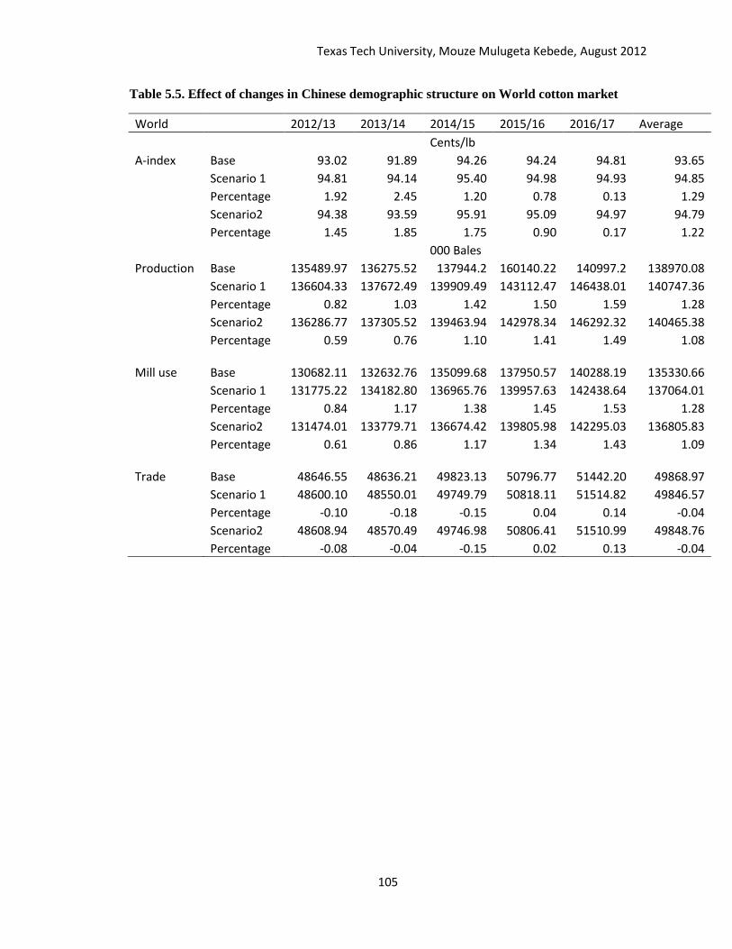
Texas Tech University, Mouze Mulugeta Kebede, August 2012
105
Table 5.5. Effect of changes in Chinese demographic structure on World cotton market
World 2012/13 2013/14 2014/15 2015/16 2016/17 Average
Cents/lb
A-index Base 93.02 91.89 94.26 94.24 94.81 93.65
Scenario 1 94.81 94.14 95.40 94.98 94.93 94.85
Percentage 1.92 2.45 1.20 0.78 0.13 1.29
Scenario2 94.38 93.59 95.91 95.09 94.97 94.79
Percentage 1.45 1.85 1.75 0.90 0.17 1.22
000 Bales
Production Base 135489.97 136275.52 137944.2 160140.22 140997.2 138970.08
Scenario 1 136604.33 137672.49 139909.49 143112.47 146438.01 140747.36
Percentage 0.82 1.03 1.42 1.50 1.59 1.28
Scenario2 136286.77 137305.52 139463.94 142978.34 146292.32 140465.38
Percentage 0.59 0.76 1.10 1.41 1.49 1.08 Mill use Base 130682.11 132632.76 135099.68 137950.57 140288.19 135330.66
Scenario 1 131775.22 134182.80 136965.76 139957.63 142438.64 137064.01
Percentage 0.84 1.17 1.38 1.45 1.53 1.28
Scenario2 131474.01 133779.71 136674.42 139805.98 142295.03 136805.83
Percentage 0.61 0.86 1.17 1.34 1.43 1.09 Trade Base 48646.55 48636.21 49823.13 50796.77 51442.20 49868.97
Scenario 1 48600.10 48550.01 49749.79 50818.11 51514.82 49846.57
Percentage -0.10 -0.18 -0.15 0.04 0.14 -0.04
Scenario2 48608.94 48570.49 49746.98 50806.41 51510.99 49848.76
Percentage -0.08 -0.04 -0.15 0.02 0.13 -0.04
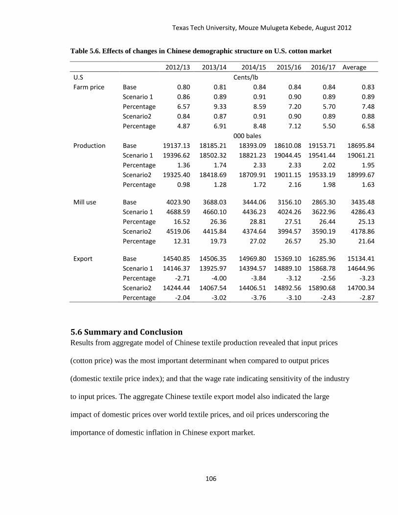
Texas Tech University, Mouze Mulugeta Kebede, August 2012
106
Table 5.6. Effects of changes in Chinese demographic structure on U.S. cotton market
2012/13 2013/14 2014/15 2015/16 2016/17 Average
U.S Cents/lb
Farm price Base 0.80 0.81 0.84 0.84 0.84 0.83
Scenario 1 0.86 0.89 0.91 0.90 0.89 0.89
Percentage 6.57 9.33 8.59 7.20 5.70 7.48
Scenario2 0.84 0.87 0.91 0.90 0.89 0.88
Percentage 4.87 6.91 8.48 7.12 5.50 6.58
000 bales
Production Base 19137.13 18185.21 18393.09 18610.08 19153.71 18695.84
Scenario 1 19396.62 18502.32 18821.23 19044.45 19541.44 19061.21
Percentage 1.36 1.74 2.33 2.33 2.02 1.95
Scenario2 19325.40 18418.69 18709.91 19011.15 19533.19 18999.67
Percentage 0.98 1.28 1.72 2.16 1.98 1.63 Mill use Base 4023.90 3688.03 3444.06 3156.10 2865.30 3435.48
Scenario 1 4688.59 4660.10 4436.23 4024.26 3622.96 4286.43
Percentage 16.52 26.36 28.81 27.51 26.44 25.13
Scenario2 4519.06 4415.84 4374.64 3994.57 3590.19 4178.86
Percentage 12.31 19.73 27.02 26.57 25.30 21.64 Export Base 14540.85 14506.35 14969.80 15369.10 16285.96 15134.41
Scenario 1 14146.37 13925.97 14394.57 14889.10 15868.78 14644.96
Percentage -2.71 -4.00 -3.84 -3.12 -2.56 -3.23
Scenario2 14244.44 14067.54 14406.51 14892.56 15890.68 14700.34
Percentage -2.04 -3.02 -3.76 -3.10 -2.43 -2.87
5.6 Summary and Conclusion Results from aggregate model of Chinese textile production revealed that input prices
(cotton price) was the most important determinant when compared to output prices
(domestic textile price index); and that the wage rate indicating sensitivity of the industry
to input prices. The aggregate Chinese textile export model also indicated the large
impact of domestic prices over world textile prices, and oil prices underscoring the
importance of domestic inflation in Chinese export market.

Texas Tech University, Mouze Mulugeta Kebede, August 2012
107
Simulation results from this study also supported the findings obtained under the
aggregate model. In general, the impact of income changes on demand for textiles is
stronger than the effect of income growth on textile production cost, thus pointing toward
an expansion of both the Chinese domestic textile and cotton sector. On the other hand,
the effect on the textile trade sector is negative, largely owing to a significant increase in
domestic textile price as a result of supply decreases and demand increases. The spillover
effect on the world and U.S market is, in most cases, expansionary causing the A-index,
world mill use, cotton production, U.S farm price, mill use, and cotton production to
increase, especially in later years of the simulation period. The trade effect, on other
hand, is negative and gets minimized in later years.
Demographic changes such as increase in elderly population and smaller family size
analyzed under scenario two have implications for textile and cotton markets. Cotton
farmers in India, other Asian countries, Argentina, and West African countries are likely
to be beneficiaries of these changes as exports of cotton is expected to grow from these
countries during the simulation period. Similar results can also be generalized regarding
the effect of demographic changes on Chinese and the U.S cotton market.
Texas Tech University, Mouze Mulugeta Kebede, August 2012
108
Chapter Six
Summary and Conclusion
This study has analyzed household textile expenditure patterns in China, taking into account fiber
choice, shopping behavior, and differences in preferences across different demographic groups.
The dissertation is motivated by the need to understand the evolution, behavior and characteristics
of Chinese consumers given the large and growing importance of Chinese textile industry on the
global market. To accomplish this task, the study used cross-sectional household data which
were obtained from a 2009 cotton consumer tracking study conducted by Cotton Council
International.
Results in regards to marginal effects of socioeconomic variables indicated that the ready-to-retire
age group tends to have a different consumption pattern than the other age groups. Consumers in
ready-to-retire age group are likely to spend more on home-textile and less on apparel compared
to the other age groups. This result disputes the long standing view that the elderly spend less on
textiles. Given the increasing proportion of the elderly consumer group, the high income elasticity
of home-textiles and double digit economic growth rate sustained by China, it appears that home-
textile marketers need to align marketing strategies that are designed to consider the elderly.
Another significant finding relates to apparel shopping behavior of Chinese households. Though
modern retail formats such as chain/ specialty stores have just started to evolve in china, attribute
they offer such as better in-store services, and a wide range of quality and fashionable products
appears to be appealing to Chinese apparel consumers. Such findings appear to mirror the retail
evolution experienced in the western developed world where the popularity of factory outlets,
discount and department stores declining over the years in favor of specialty stores.
Another important finding from this analysis relates to the potential for a decline in
dominance of China’s apparel industry in the global textile market. Though China still

Texas Tech University, Mouze Mulugeta Kebede, August 2012
109
leads the world in apparel production, recent rise in domestic labor costs has put the
industry lose its comparative advantage of lower labor cost. To retain this competitive
advantage in apparel production, however, producers need to emphasize on product
development and design, which are likely to be more profitable.
Limitations exist for this study. The data used for this analysis is from urban consumers
and is based on a one year study on household textile consumption pattern. The findings,
as a result, are limited in terms of explaining the evolution of Chinese household
consumption behavior; however the research provides a foundation for further research
for textile market in China. In addition, future research in other emerging economies such
as India and Brazil would give a better picture in understanding the global textile market.
Texas Tech University, Mouze Mulugeta Kebede, August 2012
110
References
Abernaty, F.H., J.T. Dunlop, J.H. Hammond, D. Weil(1999).The Development of the
China Apparel Industry, Harvard Center for Textile and Apparel Research.
Agnew , G.K. 1998. “LinQuad: An Incomplete Demand Systems Approach to
Demand Estimation and Exact Welfare Measures.” Thesis. Department of
Agricultural and Resource economics, University of Arizona.
Alston J.M. and Chalfant J.A. (1993). The Silence of the Lambdas: a Test of the
Almost Ideal and Rotterdam Models. American Journal of Agricultural Economics,
75: 304-313.
Amemiya, T. 1984. Tobit Models: A Survey. Journal of Econometrics, 24:3-61.
Barten, A.P. 1964. Consumer Demand Functions Under Conditions of Almost
Additive Preferences. Econometrica 32, 1-38.
_________ 1969. Maximum Likelihood estimation of a complete system of demand
equation, European economic Review 1:7-73.
Belasco, E., S. Ghosh, and Chidmi B. 2010. An Evaluation of the Soda Tax with
Multivariate Nonparametric Regressions. Selected Paper. American Agricultural
Economic Association Annual Meeting, Denver, Colorado.
Clements K.W., Selvanathan A., and Selvanathan S. (1996). Applied Demand
Analysis: A Survey. The Economic Record 72,63-81.
Christensen, L.R., Jorgenson, D.W. and Lau, L.J. (1975). Transcendental Logarthmic
Utility Functions. American Economic Review 65, 367-83.
CCI (Cotton Council International). Estimating Cotton Equivalence of Chinese End-
Use Consumption. Memo, November 2010.
Davidson, R. and J.G. MacKinnon. 1981.Several Tests for Model Specification in
Presence of Alternative Hypothesis. Econometrica, 49(3):781-793.
Deaton, A. and Muellbauer. J. 1980. An Almost Ideal Demand System. The American
Economic Review, 70, 312-326.
Deaton, Angus, and John Muellbauer. 1980. Economics and Consumer Behavior
(Cambridge: Cambridge University Press, 1980).
Dicken, P. (1998).Global Shift: Transforming the World economy. Paul
Chapman,London.
Edgerton D.L.1997. Weak Separability and the Estimation in Multistage Demand
Systems. American Journal of Agricultural Economics,79:62-79.

Texas Tech University, Mouze Mulugeta Kebede, August 2012
111
Fadiga M.L, Misra S.K. and Ramirez O.A. U.S Consumer Purchasing Decisions and
Demand for Apparel. Journal of Fashion Marketing and Management, 9(2005):1361-
2026.
Fadiga M.L, Mohanty S, Welch M, Pan S. 2008. Doha Development Agenda:
Implications for the U.S. and World Cotton Markets. The Journal of International
Trade and Economic Development, 17:135-153.
FAPRI.2001. Documentation of World Cotton Model. FAPRI-UMC Technical Data
Report 00-01.
Food and Agricultural Organization, World Apparel Fiber Consumption Survey,
various issues.
Fiber Organon. Fiber Economic Bureau, selected issues.
Gao Q. and Zhai F. Demographic Changes and Household Income in Urban China.
Paper Prepared for the 29th
General Conference of the International Association for
Research in Income and Wealth, Joensuu, Finland, August 2006.
Greene,W.H. 2007. Econometric Analysis. Upper Saddle River, N.J.: Prentice Hall.
Guilkey,D., Lovell C.A.K, and Sickles R.C. 1983. A Comparison of the Performance
of Three Flexible Functional Forms. International Economic Review 24:591-616.
Hanskul S. Understanding China’s Consumers. Deutsche Bank Research. September
2010.
Hayfield , R., and J. Racine. 2008.Nonparametric Econometrics: the NP Package.
Journal of Statistical Software 27:1-32.
Heien, D., and C. Wessells.1990. Demand Systems Estimation with Microdata: A
Censored Regression Approach. Journal of Business and Economics Statistics 8: 365-
371.
Hudson D. and Ethridge D. 2000. Income distributional impact of trade policies in a
multi market framework: a case in Pakistan. Journal of Agricultural and Applied
Economics 32(1), 49-61.
Hurd, M. 1979. Estimation in Truncated Samples When There is Hetroscedasticity.
Journal of Econometrics, 11:247-258.
International Cotton Advisory Committee (ICAC).2009. World Textile Demand.
Washington, DC.
Jones M and Hayes S.G. The Economic Determinants of Clothing Consumption in
UK 1987-2000. Journal of Fashion Marketing and Management, 6(2002):326-339.
Texas Tech University, Mouze Mulugeta Kebede, August 2012
112
Just, R.E, D.L Hueth, and A. Schmitz .2004. The Welfare Economics of Public
Policy. Edward Elgar Publishing Inc., Northampton, Massachusetts.
Klein, L.R. and H.Rubin. 1947-1948. A constant Utility Index of the Cost of Living.
Review of economic studies 15:84-87.
Klein R. L. and R.H. Spady. 1993. An Efficient Semiparametric Estimator for Binary
Response Models. Econometrica 63: 387-421.
Kim, K.,2003. U.S. Aggregate Demand for Clothing and Shoes, 1929-1994: Effects
of Nondurables Expenditures, Price and Demographic Changes. International Journal
of Consumer Studies, 27:11-125.
Kim S. and Kincade D. H. 2007. Evolution of Retail Institution Types and
Consumers’ Store Patronage Behavior: A Cross-Cultural Comparison Among
Consumers in China, India, and the United States.
LaFrance, J. T., 1990. Incomplete Demand Systems and Semilogarthmic Demand
Models. Australian Journal of Agricultural Economics, 34: 118-131.
Lafrance, J.T, Beatty T,K.M, and Pope R.D. 2006. Gorman Engle Curves for
Incomplete Demand Systems. Exploring Frontiers in Applied Economics: Essays in
Honor of Stanley R. Johnson. Berkley: Berkley electronic Press.
Lazaridis P. 2004. Demand Elastcities Derived from Consistent Estimation of
Heckman Type Models. Applied Economic Letters, 11:523-527.
Lee, J., D. Sherman, and H. Wang. Apparel Expenditiires Pattems of Elderly
Consumers: A Life-Cycle Consumption Model. Family and Consumer Science
Research Journal, 26 (December 1997): 109-147.
Lee , L. and M. M. Pitt. 1987. Micro-econometric Models of Rationing, Imperfect
Markets, and Non –negativity Constraints. Journal of econometrics 36: 89-110.
Lewbell A. 1989. Identification and Estimation of Equivalence Scales under Weak
Separability. Review of Economic Studies, 56: 311-316.
Li and Fung Research Centre .2011. China’s Apparel Market, available at
http://www.lifunggroup.com/eng/knowledge/research/industry_series19.pdf
MacDonald S., Pan S., Hudson D., Tuan F. 2011. Toward a Consumer Economy in
China: Implications of Changing Wage Policies for U.S. Cotton Exports. Selected
Paper for Presentation at the American Agricultural Economics Association annual
Meeting, Pittsburgh, July 24-26.
Martins M. F.2001. Parametric and Semiparametric Estimation of Sample Selection
Models: An Empirical Application of Female Labour Force in Portugal. Journal of
Applied Econometrics,16:23-29.

Texas Tech University, Mouze Mulugeta Kebede, August 2012
113
Mokhtari M. An Alternative Model of US Clothing Expenditures: An application of
Co- integration Techniques. The Journal of Consumer Affairs, 26(Winter 1992):305-
323.
National Bureau of Statistics of China (NBS). China Statistical Yearbook, China
Statistical Publishing House, Beijing, 2003-2009.
Nelson J.A. Individual Consumption within the Household: a Study of Expenditures
on Clothing. The Journal of Consumer Affairs, 23(Summer 1989)2:21-44.
Newey W.K., Powell J.L., Walker J.R.(1990).Semi-parametric Estimation of
Selection Models: Some Empirical Results. The American Economic
Review,80:324-328.
Pan, S., D.Hudson, M.Mutuc and D. Ethridge. Structural models of the U.S. and rest
of the world natural fiber markets. Working Paper CER 04-03, Department of
Agricultural and Applied Economics, Texas Tech University 2004(updated 2011).
Pan, S., M. Welch , S. Mohanty, D. Ethridge, M. Fadiga.2005. Chinese Tariff Rate
Quota vs. U.S. Subsidies: what affects the world Cotton Market More? Selected
Paper for Presentation at the American Agricultural Economics Association annual
Meeting, Rohde Island, July 24-27.
Pan, S., M.L. Fadiga, S. Mohanty, and M. Welch. Cotton in a Free Trade
World. Economic Inquiry, 45 (1, 2007): 188-197.
Pan. S., S. Mohanty, D. Ethridge, and M. L. Fadiga. Effects of Chinese Currency
Revaluation on World Fiber Markets. Contemporary Economic Policy, 25 (2): 185-
205, June 2006.
[PCIFibre], “Textile Fiber Demand, 2010, memo, available at
http://pcifibres.com/images/Peter%20Driscoll%20HK08%20Paper.pdf.
Pollak, Robert A., and Terence J. Wales (1978). Estimation of Complete Demand
Systems from Household Budget Data: The Linear and Quadratic Expenditure
Systems, American Economic Review 68 (June 1978), 348-359.
____________ (1992). Demand System Specification and Estimation. Oxford
University Press.
___________ (1978). Comparison of the Quadratic Expenditure system and Translog
Demand Systems with Alternative Specifications of Demographic Effects.
Econometrica 48, 595-612.
Qui L.D. 2005. China’s Textile and Clothing Industry. http://s3.amazonaws.com/zanran_storage/www.bm.ust.hk/ContentPages/18112599.pdf
Ray R. 1983. Measuring the Cost of Children.: An alternative Approach. Journal of
Public Economics.22:89-102.

Texas Tech University, Mouze Mulugeta Kebede, August 2012
114
Sam, A., and Zheng Y. 2010. Semi-parametric Estimation of Consumer Demand
Systems with Micro Data. American Journal of Agricultural Economics 92:246-257.
Shonkwiler, J. S. and S. Yen. "Two-Step Estimation of a Censored System of
Equations."'American Journal of Agricultural Economics, 81(1999): 972-982.
Stone, R. (1954). Linear expenditure Systems and Demand Analysis: An Application
to the Pattern of British Demand. Economic Journal 64, 511-27.
Sumner, D. A.2003. A quantitative simulation analysis of the impacts of U.S. cotton
subsidies on cotton prices and quantities. Mimeo, Department of Agricultural and
Resource Economics, University of California Davis.
Thiel, H. (1965). The Information Approach to demand analysis. Econometrica 33,
67-87.
UNIDO (2009). Industrial Development Report 2009, United Nations Industrial
Development Organization, Vienna, Austria.
United States Department of Agriculture (USDA). Cotton and Wool Situation and
Outlook Yearbook, various issues.
Wang F.2011. The Future of Demographic Overachiever: Long Term Implications of
the Demographic transition in China. Population and development Review
37(supplement).
Wagner J. Expenditure for Household Textiles and Textiles Home Furnishings: An
Engle curve Analysis. Home economics research Journal 15(September 1986):21-31.
Wagner J. and Mokhtari M. The Moderating effect of Seasonality on Household
Apparel Expenditure. The Journal of Consumer Affairs 34(Winter 2000):314-328.
Winakor, G. Household Textile Expenditure by Farm and City Families: Assortment
Owned, annual Expenditures, and Sources. Family and Consumer Science Research
Journal, 4(September 1975):1-26.
Yen S.T., Kan Kamhon and Jiuan S.S (2002). Household Demand for Fats and Oils:
Two-Step estimation of a Censored Demand System. Applied Economics, 14:1799-
1806.
Yen, Steven T., Biing-Hwan Lin, and David M. Smallwood (2003). “Quasi- and
Simulated Likelihood Approaches to Censored Demand Systems: Food Consumption
by Food Stamp Recipients in the United States,” American Journal of Agricultural
Economics, 85, pp. 458–478
Yen S.T., Lin, B.H. (2004). A Sample Selection Approach to Demand Systems.
Selected Paper for Presentation at the American Agricultural Economic Association,
Denver, Colorado, August 2004.
Texas Tech University, Mouze Mulugeta Kebede, August 2012
115
Zhang Z., Ching G., Gong C., Moody J, and Liu W.S. Investigation of Denim Wear
Consumption in China. Research Journal of Textiles and Apparel, 1999(3):60-6

Texas Tech University, Mouze Mulugeta Kebede, August 2012
116
Appendix A
TableA.1. Estimated parameters of participation equation for apparel model
Klein-Spady Probit
Variables Shirt Dress Other Shirt Dress Other
Intercept n/a n/a n/a 2.498**
(0.5092)
3.6099**
(0.5944)
3.135**
(0.5349)
Family size n/a n/a n/a -0.0122
(0.0312)
-0.0767*
(0.0443)
0.0097
(0.0341)
Coat price 0.0009
(0.0015)
0.0017
(0.0014)
-0.0063**
(0.0029)
0.1552**
(0.0572)
-0.0038
(0.0748)
-0.3119**
(0.0622)
Pants price -0.0007
(0.0018)
-0.0025
(0.0016)
-0.0071**
(0.0027)
-0.0599
(0.0624)
-0.1443*
(0.0779)
-0.1528**
(0.0673)
Shirt price -0.3068**
(0.0020)
0.0012
(0.0014)
0.0045
(0.0033)
-0.7223**
(0.0613)
-0.2067**
(0.0672)
-0.3577**
(0.0607)

Texas Tech University, Mouze Mulugeta Kebede, August 2012
117
TableA.1. Estimated parameters of participation equation for apparel model (continued….)
Dress price
-0.0077**
(0.0015)
-0.2557**
(0.0021)
-0.0094**
(0.0031)
-0.2269**
(0.0941)
-1.1550**
(0.1092)
-0.1328
(0.0972)
Others price -0.0008
(0.0011)
0.0002
(0.0014)
-0.3199**
(0.0019)
-0.1153
(0.0401)
-0.0912*
(0.0495)
-0.8506**
(0.0502)
Expenditure -0.0002
(0.0011)
-0.0005
(0.0011)
0.0015
(0.0017)
0.2049**
(0.0333)
0.4098**
(0.0487)
0.6164**
(0.0388)
Age 15-29
(ref: over50)
0.0310**
(0.0027)
0.0081**
(0.0022)
0.0044
(0.0058)
0.0458
(0.1068)
-0.0821
(0.1479)
-0.0538
(0.1164)
Age 30-39 0.0275** 0.0113** 0.0039 -0.0107 -0.00069 0.0348
(0.0030) (0.0027) (0.0060) (0.1210) (0.1648) (0.1315)
Age 40-49 0.0372**
(0.0031)
0.0085**
(0.0025)
0.0077
(0.0055)
-0.0812
(0.1121)
0.0044
(0.1534)
0.0002
(0.1224)
High school education ( ref:
primary education
0.0029
(0.0039)
0.0009
(0.0045)
0.0312**
(0.0053)
-0.1233
(0.1078)
0.1556
(0.1485)
-0.0538
(0.1184)
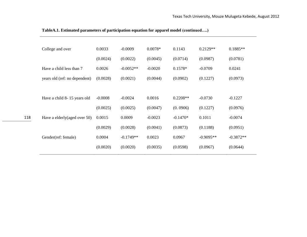
Texas Tech University, Mouze Mulugeta Kebede, August 2012
118
TableA.1. Estimated parameters of participation equation for apparel model (continued….)
College and over
0.0033
(0.0024)
-0.0009
(0.0022)
0.0078*
(0.0045)
0.1143
(0.0714)
0.2129**
(0.0987)
0.1885**
(0.0781)
Have a child less than 7
years old (ref: no dependent)
0.0026
(0.0028)
-0.0052**
(0.0021)
-0.0020
(0.0044)
0.1578*
(0.0902)
-0.0709
(0.1227)
0.0241
(0.0973)
Have a child 8- 15 years old
-0.0008
(0.0025)
-0.0024
(0.0025)
0.0016
(0.0047)
0.2208**
(0. 0906)
-0.0730
(0.1227)
-0.1227
(0.0976)
Have a elderly(aged over 50) 0.0015
(0.0029)
0.0009
(0.0028)
-0.0023
(0.0041)
-0.1470*
(0.0873)
0.1011
(0.1188)
-0.0074
(0.0951)
Gender(ref: female) 0.0004
(0.0020)
-0.1749**
(0.0020)
0.0023
(0.0035)
0.0967
(0.0598)
-0.9095**
(0.0967)
-0.3872**
(0.0644)
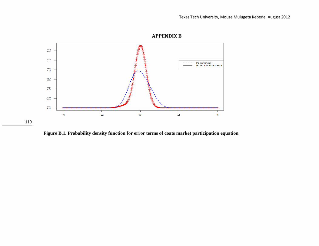
Texas Tech University, Mouze Mulugeta Kebede, August 2012
119
APPENDIX B
Figure B.1. Probability density function for error terms of coats market participation equation
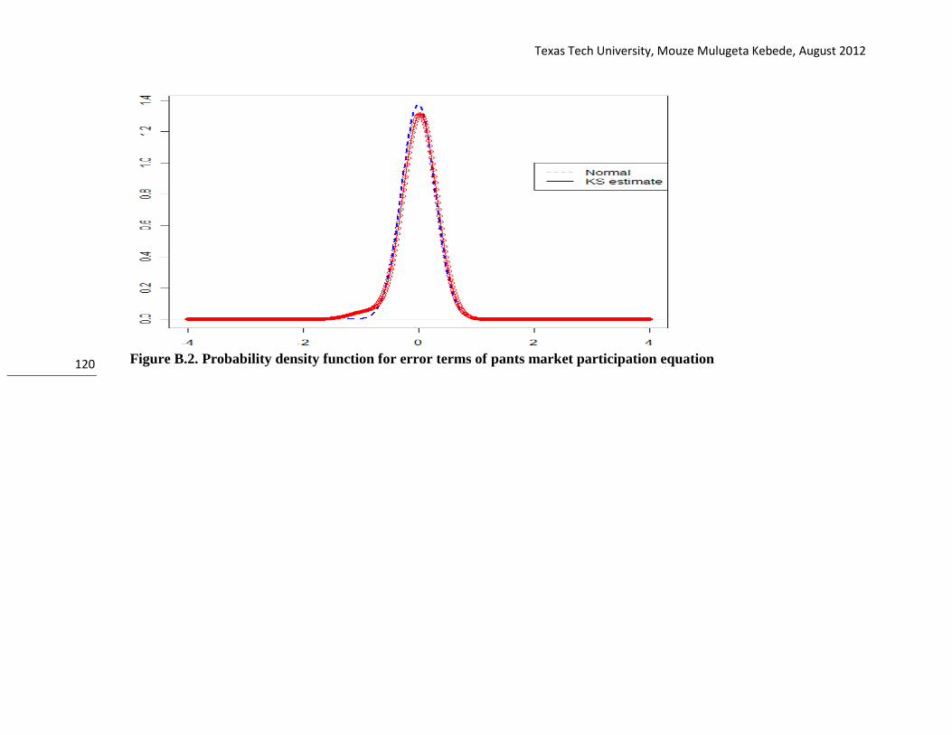
Texas Tech University, Mouze Mulugeta Kebede, August 2012
120
Figure B.2. Probability density function for error terms of pants market participation equation


![Textile Technology [Read-Only]textile.yazd.ac.ir/ms.ahmadi/Downloads/Textile Technology/Textile... · Textile Technology (Pictures) Edited by: M. S. Ahmadi Textile Technology 1 Yazd](https://img.pdfslide.net/doc/110x75/5e786641131316263558e076/textile-technology-read-only-technologytextile-textile-technology-pictures.jpg)