Embed Size (px)
Citation preview

Graduate Theses, Dissertations, and Problem Reports
2020
Three Essays on Health Economics and Policy Evaluation Three Essays on Health Economics and Policy Evaluation
Shishir Shakya West Virginia University, [email protected]
Follow this and additional works at: https://researchrepository.wvu.edu/etd
Part of the Applied Statistics Commons, Behavioral Economics Commons, Business Analytics
Commons, Clinical Trials Commons, Community Health and Preventive Medicine Commons, Data Science
Commons, Econometrics Commons, Economic Policy Commons, Health Economics Commons, Health
Policy Commons, Health Services Research Commons, Insurance Commons, Longitudinal Data Analysis
and Time Series Commons, Medicine and Health Commons, Multivariate Analysis Commons, Policy
Design, Analysis, and Evaluation Commons, Public Economics Commons, Public Policy Commons,
Regional Economics Commons, and the Vital and Health Statistics Commons
Recommended Citation Recommended Citation Shakya, Shishir, "Three Essays on Health Economics and Policy Evaluation" (2020). Graduate Theses, Dissertations, and Problem Reports. 7767. https://researchrepository.wvu.edu/etd/7767
This Dissertation is protected by copyright and/or related rights. It has been brought to you by the The Research Repository @ WVU with permission from the rights-holder(s). You are free to use this Dissertation in any way that is permitted by the copyright and related rights legislation that applies to your use. For other uses you must obtain permission from the rights-holder(s) directly, unless additional rights are indicated by a Creative Commons license in the record and/ or on the work itself. This Dissertation has been accepted for inclusion in WVU Graduate Theses, Dissertations, and Problem Reports collection by an authorized administrator of The Research Repository @ WVU. For more information, please contact [email protected].

Graduate Theses, Dissertations, and Problem Reports
2020
Three Essays on Health Economics and Policy Evaluation Three Essays on Health Economics and Policy Evaluation
Shishir Shakya
Follow this and additional works at: https://researchrepository.wvu.edu/etd
Part of the Applied Statistics Commons, Behavioral Economics Commons, Business Analytics
Commons, Clinical Trials Commons, Community Health and Preventive Medicine Commons, Data Science
Commons, Econometrics Commons, Economic Policy Commons, Health Economics Commons, Health
Policy Commons, Health Services Research Commons, Insurance Commons, Longitudinal Data Analysis
and Time Series Commons, Medicine and Health Commons, Multivariate Analysis Commons, Policy
Design, Analysis, and Evaluation Commons, Public Economics Commons, Public Policy Commons,
Regional Economics Commons, and the Vital and Health Statistics Commons

Three Essays on Health Economics and
Policy Evaluation
Shishir Shakya
Dissertation submittedto the John Chambers College of Business and Economics
at West Virginia University
in partial fulfillment of the requirementsfor the degree of
Doctor of Philosophy inEconomics
Jane E. Ruseski, Ph.D., ChairJoshua C. Hall, Ph.D.
Feng Yao, Ph.D.Bradley S. Price, Ph.D.
Department of Economics
Morgantown, West Virginia2020
Keywords: Prescription Opioid, Prescription Drug Monitoring Program, RetailOpioid Prescription, Medicaid, Program Evaluation, Policy Learning, Causal
Inference and Machine Learning
Copyright 2020 Shishir Shakya

Abstract
Three Essays on Health Economics and Policy Evaluation
Shishir Shakya
This dissertation consists of three essays on U.S. Health care policy. Each para-graph below refers to the three abstracts for the three chapters in this dissertation,respectively.
I provide quantitative evidence on how much Prescription Drug Monitoring Pro-grams (PDMPs) affects the retail opioid prescribing behaviors. Using the AmericanCommunity Survey (ACS), I retrieve county-level high dimensional panel data setfrom 2010 to 2017. I employ three separate identification strategies: difference-in-difference, double selection post-LASSO, and spatial difference-in-difference. I com-pare how the retail opioid prescribing behaviors of counties, that are mandatory forprescribers to check the PDMP before prescribing controlled substances (must-accessPDMPs), vary from the counties where such a PDMP check is voluntary. I findmust-access PDMP reduces about seven retail opioid prescriptions dispensed per 100persons per year in each county. But, when I compare must-access PDMPs countieswith bordering counties without such law, I find a reduction of three retail opioid pre-scriptions dispensed per 100 persons per year suggesting the possibility of spilloversof retail opioid prescribing behaviors.
As of 2019, all U.S. states, except Missouri, have enacted voluntary PrescriptionDrug Monitoring Programs (PDMPs). In response to the relatively low uptake ofvoluntary access, several states have strengthened their PDPMs by requiring providersto access information regarding prescription drug use under certain circumstances.These “must-access” PDPMs require states to view a patient’s prescription history tofacilitate the detection of suspicious prescription and utilization behaviors. This paperdevelops causal evidence of the effectiveness of “must-access” PDPM laws in reducingprescription opioid overdose death rates relative to voluntary PDMP states. I findthat PDMPs are ineffective in reducing prescription opioid overdose deaths overall,but the effects are heterogeneous across states with “must-access” PDMP states. Ifind that marijuana and naloxone access laws, poverty level, income, and educationconfound the impact of must-access PDMPs on prescription opioid overdose deaths.
The optional provision of Medicaid expansion, through the Affordable Care Act(ACA), has triggered a national debate among diverse stakeholders regarding the im-pacts of Medicaid coverage on various dimensions of public health, costs, and benefits.Randomized experiments like the Rand Health Insurance Experiment and the OregonHealth Insurance Experiment have generated some credible estimates of the averagetreatment effects of insurance access. However, identical policy interventions canhave heterogeneous effects on different subpopulations. This paper uses data fromthe Oregon Health Insurance Experiment to estimate the heterogeneous treatment

effects of access to Medicaid on health care utilization, preventive care utilization,financial strain, and self-reported physical and mental health. I detect heterogeneoustreatment effects using a cluster-robust generalized random forest, a causal machinelearning approach. I find that the impact of Medicaid is more pronounced amongrelatively older non-elderly and poorer households, consistent with standard adverseselection theory. Furthermore, I implement the “efficient policy learning,” anothermachine learning strategy, to identify policy changes that prioritize providing Medi-caid coverage to the subgroups that are likely to benefit the most. On average, theproposed reforms would improve the average probability of outpatient visits, pre-ventive care use, overall health outcomes, having a personal doctor and clinic, andhappiness by a range of 2% to 9% over a random assignment baseline. These findingshelp design Medicaid Section 1115 waiver.

Three Essays on Health Economics and Policy Evaluation
by
Shishir Shakya
Dissertation submitted to theJohn Chambers College of Business and Economics
at West Virginia Universityin partial fulfillment of the requirements for the degree of
Doctor of Philosophyin
Economics
Department of Economics
APPROVAL OF THE EXAMINING COMMITTEE
Joshua C. Hall, Ph.D.
Feng Yao, Ph.D.
Bradley S. Price, Ph.D.
Jane E. Ruseski, Ph.D., Chair
Date
iv

v
Dedication
I dedicate this dissertation to my wife Gita, son Soham, and my family in Nepal.
Thank you for letting me chase my dreams.

vi
Acknowledgements
I want to thank my advisors, Dr. Jane E. Ruseski and Dr. Joshua C. Hall, for the
continued support throughout these years. I would also like to thank my committee
members, Dr. Feng Yao and Dr. Bradley S. Price, for their invaluable feedback.
I appreciate Prof. Bob Reed; without his support, this journey of PhD. was never
a possibility for me. I also acknowledge Mr. Ashutosh Mani Dixit; he persistently
motivated and helped me to pursue doctoral education. My sincere thanks go to Dr.
Randall Jackson; he is my rock. The support that I have received from the Regional
Research Institute family is beyond the words of expressions. My forever listening
ears are Alexandre Scarcioffolo, Sultan Aziz, and Eduardo Minuci. Thank you for
being there in good and in bad times. Dr. Amir Neto and Dr. Shree Baba Pokherel
were my guide-posts who smoothen the rugged terrain of a Ph.D. by always timely
guiding me on what to expect next and how to handle each Ph.D. requirements. My
sincere gratitude goes to Dr. Alicia Morgan Plemmons, who continuously mentored
me in the transition phases of my Ph.D. and job market seasons.

vii
Table of Contents
Approval Page iv
List of Figures ix
List of Tables x
1 County Level Assessment of Prescription Drug Monitoring Programand Opioid Prescription Rate 11.1 Introduction . . . . . . . . . . . . . . . . . . . . . . . . . . . . . . . . 11.2 Data . . . . . . . . . . . . . . . . . . . . . . . . . . . . . . . . . . . . 51.3 Methodology . . . . . . . . . . . . . . . . . . . . . . . . . . . . . . . 8
1.3.1 Difference-in-Difference with Fixed Effects and Clustered Standard-Errors . . . . . . . . . . . . . . . . . . . . . . . . . . . . . . . 8
1.3.2 High Dimensional Features and Unknown Data Generating Pro-cess . . . . . . . . . . . . . . . . . . . . . . . . . . . . . . . . 9
1.3.3 Double Selection Post LASSO . . . . . . . . . . . . . . . . . . 101.3.4 Managing Unobservable with Spatial Difference-in-Difference . 12
1.4 Results . . . . . . . . . . . . . . . . . . . . . . . . . . . . . . . . . . . 121.5 Conclusion . . . . . . . . . . . . . . . . . . . . . . . . . . . . . . . . . 16
2 Impact of Must-access Prescription Drug Monitoring Program onPrescription Opioid Overdose Death Rates 182.1 Introduction . . . . . . . . . . . . . . . . . . . . . . . . . . . . . . . . 182.2 Prescription Drug Epidemic . . . . . . . . . . . . . . . . . . . . . . . 222.3 Literature Review . . . . . . . . . . . . . . . . . . . . . . . . . . . . . 242.4 Empirical Strategies . . . . . . . . . . . . . . . . . . . . . . . . . . . 27
2.4.1 Two-way Fixed Effect Difference-in-Differences Framework . . 272.4.2 Two-way Fixed Effect Difference-in-Differences Framework with
LASSO . . . . . . . . . . . . . . . . . . . . . . . . . . . . . . 282.4.3 Event Study Framework . . . . . . . . . . . . . . . . . . . . . 292.4.4 Generalized Synthetic Control . . . . . . . . . . . . . . . . . . 30
2.5 Data . . . . . . . . . . . . . . . . . . . . . . . . . . . . . . . . . . . . 332.6 Results . . . . . . . . . . . . . . . . . . . . . . . . . . . . . . . . . . . 37

TABLE OF CONTENTS viii
2.6.1 Main Results . . . . . . . . . . . . . . . . . . . . . . . . . . . 372.6.2 A Nationwide Time Trends in Rx Opioid . . . . . . . . . . . . 412.6.3 State-level Impact of Must-access PDMPs . . . . . . . . . . . 422.6.4 Validity: Consistency using High Dimensional Covariates . . . 43
2.7 Discussion and Conclusion . . . . . . . . . . . . . . . . . . . . . . . . 45
3 Heterogeneous Treatment Effects of Medicaid and Efficient Policies 483.1 Introduction . . . . . . . . . . . . . . . . . . . . . . . . . . . . . . . . 483.2 Oregon Health Insurance Experiment . . . . . . . . . . . . . . . . . . 543.3 Approaches to Health Insurance & Health Outcomes . . . . . . . . . 563.4 Empirical Strategy . . . . . . . . . . . . . . . . . . . . . . . . . . . . 60
3.4.1 Identification . . . . . . . . . . . . . . . . . . . . . . . . . . . 603.4.2 Mean Comparison of Demographics . . . . . . . . . . . . . . . 613.4.3 Intent to Treat Effect of Lottery . . . . . . . . . . . . . . . . . 623.4.4 Local Average Treatment Effect of Lottery . . . . . . . . . . . 633.4.5 Heterogeneous Treatment Effects . . . . . . . . . . . . . . . . 643.4.6 Cluster-robust Random Forest . . . . . . . . . . . . . . . . . . 673.4.7 Estimation of Treatment Policies . . . . . . . . . . . . . . . . 70
3.5 Results . . . . . . . . . . . . . . . . . . . . . . . . . . . . . . . . . . . 723.5.1 Pre-treatment Comparison of Demographic Characteristics . . 733.5.2 ITT, LATE and Heterogeneous Treatment Effects . . . . . . . 733.5.3 Efficient Policies . . . . . . . . . . . . . . . . . . . . . . . . . 88
3.6 Discussion and Conclusion . . . . . . . . . . . . . . . . . . . . . . . . 92
A Causal Machine Learning Approaches 96
B Variable Importance 101
C Efficient Policies 102

ix
List of Figures
1.1 Retail Opioid Dispensed per 100 Persons per Year, 2017 . . . . . . . 51.2 State Requiring Prescribers to Check the PDMP Before Prescribing
Controlled Substances . . . . . . . . . . . . . . . . . . . . . . . . . . 71.3 Bordering Counties, 2017 . . . . . . . . . . . . . . . . . . . . . . . . . 13
2.1 Rx Opioid-related Overdose Death per 100,000 Population . . . . . . 342.2 State Requiring Prescribers to Check the PDMP Before Prescribing
Controlled Substances. . . . . . . . . . . . . . . . . . . . . . . . . . . 352.3 Estimated Impact of Must-access PDMP on Age-adjusted Rx Opioid
Overdose Death Rate per 100,000 Population for Years Before, During,and After Adoption, (Based on Event Study) . . . . . . . . . . . . . . 38
2.4 Estimated Impact of Must-access PDMP on Age-adjusted Rx OpioidOverdose Death Rate per 100,000 Population for Years Before, During,and After Adoption, (Based on Generalized Synthetic Control Study) 40
2.5 Factor and Factor Loadings . . . . . . . . . . . . . . . . . . . . . . . 422.6 State-level Impact of Must-access PDMPs . . . . . . . . . . . . . . . 43
3.1 A Classification Tree for Survivors of the Titanic . . . . . . . . . . . 663.2 Health Care and Preventive Care Utilization . . . . . . . . . . . . . . 793.3 Financial Strain . . . . . . . . . . . . . . . . . . . . . . . . . . . . . . 823.4 Self-reported Health . . . . . . . . . . . . . . . . . . . . . . . . . . . 863.5 Potential Mechanism for Improved Health . . . . . . . . . . . . . . . 893.6 Efficient Policy to Improve Outpatient Visits . . . . . . . . . . . . . . 91
C.1 Efficient Policy to Improve the Blood Cholesterol Check Participation 102C.2 Efficient Policy to Improve Blood Tests Participation for High Blood
Sugar/Diabetes . . . . . . . . . . . . . . . . . . . . . . . . . . . . . . 103C.3 Efficient Policy to Improve Mammogram Test Participation for Women 103C.4 Efficient Policy to Improve Pap Test Participation for Women . . . . 104C.5 Efficient Policy to Improve Self-reported Health . . . . . . . . . . . . 104C.6 Efficient Policy to Improve to have Usual Place of Clinic-based Care . 105C.7 Efficient Policy to Improve to have a Personal Doctor . . . . . . . . . 105C.8 Efficient Policy to Improve to Post Health-care Service Happiness . . 106

x
List of Tables
1.1 Impacts of Must-access PDMP on Retail Opioid Prescriptions Dispensed 141.2 Impacts of Must-access PDMP on Retail Opioid Prescriptions Dis-
pensed, Spatial Contiguity . . . . . . . . . . . . . . . . . . . . . . . . 15
2.1 Descriptive Statistics (Pooled Across the State from 1999 to 2017) . . 362.2 Impact of Must-access PDMPs on Age-adjusted Rx Opioid Overdose
Death Rate per 100,000 Population . . . . . . . . . . . . . . . . . . . 372.3 Impact of Must-access PDMPs on Age-adjusted Rx Opioid Overdose
Death Rate per 100,000 Population (Variables Selection on High Di-mensional Covariates) . . . . . . . . . . . . . . . . . . . . . . . . . . 44
3.1 Pre-treatment Comparison of Demographic Characteristics . . . . . . 743.2 Health Care Utilization . . . . . . . . . . . . . . . . . . . . . . . . . . 773.3 Financial Strain . . . . . . . . . . . . . . . . . . . . . . . . . . . . . . 813.4 Self-reported Health . . . . . . . . . . . . . . . . . . . . . . . . . . . 853.5 Potential Mechanism for Improved Health . . . . . . . . . . . . . . . 883.6 Estimate of the Utility Improvement of Various Policies Over Baseline. 90
B.1 Variable Importance . . . . . . . . . . . . . . . . . . . . . . . . . . . 101

1
Chapter 1
County Level Assessment of
Prescription Drug Monitoring
Program and Opioid Prescription
Rate
1.1 Introduction
Deaths related to overdoses of opioids drugs, including both prescription opioid
drugs and illicit opioids such as heroin and illicitly manufactured fentanyl, are rising
in the United States, especially after 2010. On average, 130 Americans die every day
from an opioid overdose (CDC, 2019). Compared to 1999, prescription-drug sales
have quadrupled in the United States (CDC, 2019), leading to a 40 percent increase
in prescription drug overdose deaths.
Abuse of prescription opioids drugs is highest compared to other variants of pre-
scription drugs. National Center on Addiction and Substance Abuse (2014) esti-
mates one in five Americans above 12-year ages misused prescription opioid drugs in
their lifetime, and more than one in four new initiates of illicit drug users started
with prescription opioid drug abuse. National Center on Addiction and Substance
Abuse (2015) estimates 119 million Americans aged 12 or older used prescription

Shishir Shakya Chapter 1. County-Level Assessment of PDMP and Opioid Rx Rate 2
psychotherapeutic drugs in the past year, representing 44.5 percent of the popu-
lation and 18.9 million people aged 12 or older (7.1 percent) misused prescription
psychotherapeutic drugs in the past year. National Center on Addiction and Sub-
stance Abuse (2015) highlights several contributing factors to the prescription opioid
drug epidemic, namely the advancement of new drug therapies, prescribing practices,
internet pharmacies, expansion of insurance coverage, pharmaceutical advertisement,
increased availability, medication and prescription pad theft, employee pilferage.
Opioid-dependent abusers steal, street purchase from a friend or relative, and
doctor-shop to obtain prescription opioid drugs for non–medical use. Physicians rep-
resent the primary source for prescription opioid opioids for those who obtain pre-
scription opioids through their own prescriptions (Jones et al., 2014). In contrast,
pharmacists and physicians claim doctor shopping as the leading source for opioid
abusers to get prescription opioid opioids (National Center on Addiction and Sub-
stance Abuse, 2015) and is an indirect channel of supply source for street dealers
(Inciardi et al., 2009).
As policy responses to the escalating rates of opioid abuse and overdose death
rates, the US policymakers have tried a variety of state-level policies like quantitative
prescription limits, patient identification requirements, doctor-shopping restrictions,
Prescription Drug Monitoring Program (henceforth PDMP or PDMPs), provisions
related to tamper-resistant prescription forms, and pain-clinic regulations (Meara
et al., 2016). The CDC has been promoting PDMPs as the best defense against the
current impending crisis (Birk and Waddell, 2017).
As of 2019, 49 US states, along with the District of Columbia and the US territory
of Guam has implemented some form of PDMPs. Except for the state of Missouri1,
all the US states have adopted voluntary PDMP. In contrast, few other states have
enacted a so-called “mandatory” or must-access PDMP. Unlike voluntary PDMP, the
must-access PDMP states abide by the law to collect data on controlled substance
1St. Louis County that accounts for more than half of Missouri’s population has implementedtheir unique PDMP and appeal to other counties and cities in Missouri to conjoin (PDMPTTAC,2019).

Shishir Shakya Chapter 1. County-Level Assessment of PDMP and Opioid Rx Rate 3
prescriptions that doctors have written for patients. The must-access PDMP states
allow authorized individuals to view a patient’s prescription history to facilitate the
detection of suspicious prescriptions and utilization behaviors. The PDPMs varies by
state along several dimensions2 and also evolve over time3.
Differentiating among voluntary and must-access PDMPs is crucial to understand
how these programs affect the prescribing rate. For example, when New York imple-
mented a must-access PDMP in 2013, the number of registrants increased fourteen-
fold, and the number of daily queries rose from fewer than 400 to more than 40,000
(PDMP Center of Excellence, 2016). Similarly, in Kentucky, Tennessee, and Ohio,
implementing a “must access” provision increased by order of magnitude the number
of providers registered and the number of queries received per day (PDMP Center of
Excellence, 2016). In contrast, in the first year after a voluntary PDMP was estab-
lished in Florida, a state with a well-publicized opioid misuse problem, fewer than one
in ten physicians had even created a login for the system (Electronic-Florida Online
Reporting of Controlled Substances Evaluation, 2014).
In this paper, I am quantifying to what extent these must-access PDMPs change
the opioid prescribing behavior. This research question is a crucial policy-relevant
issue because the risk of an opioid use disorder, overdose, and death from prescription
opioids are susceptible to the opioid prescribing rate.
Several papers relate the reduction of an opioid prescription to heroin crime
(Alpert et al., 2017; Evans et al., 2018b; Kilby, 2015; Lankenau et al., 2012; Mal-
latt, 2018; Meinhofer, 2018b). While another strand of literature relates must-access
PDMP to overdosages and overdosages death rates (Buchmueller and Carey, 2018;
Meara et al., 2016; Meinhofer, 2018b). However, in this paper, I provide several
2States can differ in who may access the database (e.g., prescribers, dispensers, law enforcement),in the agency that administers the PDMP (e.g., department of health, pharmacy boards), in thecontrolled substances (CS) that are reported (e.g., some do not monitor CS-V), in the timelinessof data reporting (e.g., daily, weekly), in how to identify and investigate cases of potential doctorshoppers (e.g., reactive, proactive), and on whether prescribers are required to query the database(Meinhofer, 2018a).
3Initially, several states implemented paper-based PDMPs. Still, eventually, these and othersshifted to electronic-based PDMPs (Meinhofer, 2018a).
Shishir Shakya Chapter 1. County-Level Assessment of PDMP and Opioid Rx Rate 4
unique contributions − first, this paper study of impacts of must-access PDMPs on
the retail opioid prescribing rate. Several studies exist to answer similar questions
(Strickler et al., 2019; Rutkow et al., 2015; Schieber et al., 2019), but these studies
are descriptive. See Ponnapalli et al. (2018) for a systematic literature review of Pre-
scription Drug Monitoring Programs too. However, I contribute to quantifying the
impacts of must-access PDMPs on the opioid prescribing rate.
Second, this paper is first to exploit the county level variations of the retail opioid
prescribing rate. Several studies provide state-level analysis of PDMPs on various
outcomes of interests, and this is because PDMPs are state-level law. However, the
county-level analysis offers a more granular summary by capturing the county level
heterogeneity on how these state-level PDMP laws change the outcome of interest.
Third, I also utilize the two-way fixed effect difference-in-difference econometric
approach with two novel identification strategies using US counties-level panel data
spanning from 2010 to 2017. The first approach is the double selection post-LASSO −
a causal-machine learning method − to control observable characteristics. The second
approach exploits spatial contiguity to control for unobservables characteristics, pos-
sibly. The PDMPs are economic policy variables that are likely not to be randomly
assigned. Therefore several observable characteristics could confound the PDMPs
law and opioid prescribing rate. These observable characteristics can be the social,
economic, and demographic profiles of counties along with several other state-level
laws like Medicaid expansion, marijuana law, good Samaritan law, Naloxone access
laws. The double selection post-LASSO allows selecting observable controls that af-
fect PDMPs and prescribing rates. However, this method is likely not to properly
unobservable. I compare the prescribing rate among must-access PMDP counties,
which the bordering counties without must-access PMDP.
I find that must-access PDMPs reduce seven retail opioid prescriptions dispensed
per 100s persons per county per year. However, when comparing the prescribing
rate among must-access PMDP counties, which the bordering counties without must-
access PMDP, I find about three retail opioid prescriptions dispensed per 100s persons

Shishir Shakya Chapter 1. County-Level Assessment of PDMP and Opioid Rx Rate 5
per county per year. Since the prescribing rate in boarding counties is lower than over-
all counties, it suggests it is likely that the prescribing rate from must-access PDMPs
counties spillovers to bordering counties that do not have must-access PDMPs.
Section 1.2 explores the data. Section 1.3 layouts two-way fixed effect difference-
in-difference econometric approach along with the double selection post LASSO and
spatial methods. Section 1.4 provides the results and section 1.5 concludes the results.
1.2 Data
I web-scrape CDC website to acquire data of the retail opioid prescriptions dis-
pensed per 100 persons per year4 from 2006 to 2017. CDC estimates prescribing rates
using the IQVIA Xponent data set.
Figure 1.1: Retail Opioid Dispensed per 100 Persons per Year, 2017
Source: https://www.cdc.gov/drugoverdose/maps/rxrate-maps.html
4Note that retail opioid prescriptions dispensed per 100 persons per year index is different fromthe morphine milligram equivalent (MME) per person or the number of opioids prescribed perperson.

Shishir Shakya Chapter 1. County-Level Assessment of PDMP and Opioid Rx Rate 6
IQVIA Xponent is based on a sample of approximately 50,000 retail (non-hospital)
pharmacies, which dispense nearly 90% of all retail prescriptions in the United States.
For this database, a prescription is an initial or refill prescription dispensed at a retail
pharmacy in the sample and paid for by commercial insurance, Medicaid, Medicare,
or cash or its equivalent. This database does not include mail order pharmacy data.
IQVIA Xponent data set uses the National Drug Code to identify opioid prescrip-
tions, which include buprenorphine, codeine, fentanyl, hydrocodone, hydromorphone,
methadone, morphine, oxycodone, oxymorphone, propoxyphene, tapentadol, and tra-
madol. However, the IQVIA Xponent data set excludes cough and cold formulations
containing opioids and buprenorphine that are typically used to treat opioid use dis-
order. Also, methadone dispensed through methadone maintenance treatment pro-
grams is not included in the IQVIA Xponent data. A lack of available data in IQVIA
Xponent may indicate that the county had no retail pharmacies, the county had no
retail pharmacies sampled, or the prescription volume was erroneously attributed to
an adjacent, more populous county according to the sampling rules used.
For the calculation of prescribing rates, numerators are the total number of opioid
prescriptions dispensed in a county in a given year, and the denominator is the annual
resident population denominator estimates obtained from the US Census Bureau.
Figure 1.1 shows US opioid prescribing rate maps in 2017, where rates are classified
by the Jenkse natural breaks classification method into four groups using the 12-year
range of data (2006 to 2017) to determine the class breaks.
I retrieve the list of states that require prescribers to check the PDMP before
prescribing controlled substances or must-access PDMP and the PDMP enactments
date from the pdaps.org website. Figure 1.2 is a visual representation of state and
timing of states that enacted must-access PDMP and the state with only voluntary
PMDPs.
Using the Application Programming Interface of Census from the “censusapi” R
package, I retrieve all the social, economic, housing, and demographic data profile
of each county in the US from the five-year American Community Survey from 2010

Shishir Shakya Chapter 1. County-Level Assessment of PDMP and Opioid Rx Rate 7
Figure 1.2: State Requiring Prescribers to Check the PDMP Before PrescribingControlled Substances
Source: http://pdaps.org/
to 2017. Then, I only include variables that are consistently available from 2010
to 2017. I then deleted variables that are a linear combination of each other and
also remove furthermore highly correlated variables. This process, finally, retains 90
different social, economic, housing, and demographic data profiles of each county.
I also retrieve state-level laws like Good Samaritan Laws and Naloxone Access
Law from pdaps.org website. I use procon.org to access the Marijuana Law (medi-
cal or/and recreational possession of Marijuana). States with the Good Samaritan
Law provide immunity from prosecution for possessing a controlled substance while
seeking help for himself or another person experiencing an overdose. The state with

Shishir Shakya Chapter 1. County-Level Assessment of PDMP and Opioid Rx Rate 8
Naloxone Access Law provides naloxone and other opioid overdose prevention services
to individuals who use drugs, their families and friends, and service providers, includ-
ing education about overdose risk factors, signs of overdose, appropriate response,
and administration of naloxone. As of 2016, 48 states have authorized some variant
of a naloxone access law, and 37 states have passed a drug overdose good samaritan
law (Ayres and Jalal, 2018).
1.3 Methodology
1.3.1 Difference-in-Difference with Fixed Effects and Clus-
tered Standard-Errors
I begin the analysis by showing if there is a significant difference in retail opioid
prescriptions dispensed per 100 persons between the counties of the state that have
a must-access prescription drug monitoring program (PDMPs henceforth) with the
counties of the state that don’t have such program. For this, I use a simple difference-
in-difference model with county and year fixed effects while clustering the standard
errors in-state levels.
Yit = c+ δDit + αi + ςt + εit (1.1)
where, Yit is retail opioid prescriptions dispensed per 100 persons per year; c is the
intercept, Dit is the treatment indicator and equals 1 after state i has been exposed to
the treatment (must-access PDMP) and equals 0 otherwise; δ is the average treatment
effect, αi and ζt are additive individual state and year fixed effects respectively. One
should expect a negative and significant value of δ, which would suggest the PDMP is
successful in reducing retail opioid prescriptions dispensed. However, a positive and
significant δ shows that states with PDMP have higher retail opioid prescriptions
dispensed rates than in comparison states that do not have must-access PDMP.

Shishir Shakya Chapter 1. County-Level Assessment of PDMP and Opioid Rx Rate 9
1.3.2 High Dimensional Features and Unknown Data Gen-
erating Process
Studies that examine the impact of the must-access PDMPs on the retail opioid
prescriptions dispensed are likely to suffer the endogeneity. The endogeneity leads
to either over or underestimation of the effects of must-access PDMPs on the retail
opioid prescriptions dispensed. The endogeneity arises because must-access PDMP
enactment is a policy response to the escalating opioid-related overdose death rate
and opioid prescribing behavior.
The equation 2.1 produces an incomplete picture of the relationship between retail
opioid prescriptions dispensed and must-access PDMP. Since the policy/treatment
variable is PDMP is a non-randomly assigned economic variable. The socio-economic
and demographic profile of each county could likely affect both retail opioid pre-
scriptions and must-access PDMP. Furthermore, literature has shown that Medicaid
expansion, marijuana law, good Samaritan law, Naloxone access laws have a diverse
effect on the demand for prescription opioids.
Failure to conditioning these confounders can lead to omitted variable bias. How-
ever, over-controlling leads to loss of efficiency of estimates. The actual data gener-
ating a process that explains the relationship between the must-access PDMPs and
the opioid prescribing rate is unknown to the researcher. However, one can use gen-
eral economic intuition to guide the variable selection that is standard in the litera-
ture. However, the actual data generating process (DGP) might comprise the various
transformation of these observable confounders, for example, lags, higher-order poly-
nomials, and interactions. Including and controlling for all these transformations
may not be feasible because the covariates space can increase exponentially with high
dimensional data.
Hence, the primary goal is to inference the low-dimensional parameter from the
high-dimensional nuisance parameter, which comprises to solve auxiliary prediction

Shishir Shakya Chapter 1. County-Level Assessment of PDMP and Opioid Rx Rate 10
problem quite well. Consider the following outcomes yi as a partially linear model:
yi = diα0 + g (zi) + ξi, E [ξi|zi, di] = 0
di = m (zi) + vi, E [vi|zi] = 0(1.2)
where we have a sample of i = 1, . . . , n independent observation, d is policy/treatment
variable as “must-access” PDMPs possibly non-randomly assigned an economic vari-
able. The α0 is the target parameter of interest, which answers the portion of
variations in outcome variable due to the changes in policy variables. zi is a high-
dimensional vector of other controls or confounders. The high-dimensional vector of
controls is in zi and collected from the social, economic, housing, and demographic
data profile from the American Community Survey for each county from 2010 to
2017. It is plausible to define that some of those features are a common cause for the
existence of “must-access” PDMP and opioid prescription, and m0 6= 0, typically in
the case of observational studies. m0 = 0 would suggest that the policy variable is
randomly assigned.
1.3.3 Double Selection Post LASSO
Lets consider linear combinations of control terms xi = P (zi) to approximate
g (zi) and m (zi). The list xi = P (zi) could be composed of many transformations
of elementary regressors zi such as B-splines, dummies, polynomials, and various
interactions. Having many controls poses a challenge of estimation and inference,
therefore, to avoid such we assume the sparsity assumption that only a few among
many variables in the zi explains outcomes yi.
yi = diα0 + x′iβg0 + rgi︸ ︷︷ ︸g(zi)
+ξi
di = x′iβm0 + rmi︸ ︷︷ ︸m(zi)
+vi
(1.3)
The sparsity then relates to x′iβg0 and x′iβm0 approximate g (zi), and m (zi) that
Shishir Shakya Chapter 1. County-Level Assessment of PDMP and Opioid Rx Rate 11
requires only a small number of non-zero coefficients to render corresponding approx-
imation errors rgi and rmi.
An appealing method to estimate the sparse parameter from a high-dimensional
linear model is the Least Absolute Shrinkage and Selection Operator (LASSO) (Tib-
shirani, 1996). LASSO simultaneously performs model selection and coefficient esti-
mation by minimizing the sum of squared residuals plus a penalty term. The penalty
term penalizes the size of the model through the sum of absolute values of coefficients.
Let me define a feasible variable selection via LASSO for outcome variable and
policy or treatment variable. Here, we change the notation as the outcome, and the
policy variable takes the following form:
yi = xiβ1 + ri+︸ ︷︷ ︸f(zi)
εi
di = xiβ2 +mi+︸ ︷︷ ︸f(zi)
εi(1.4)
moreover, LASSO estimator is defined as the solution to:
minβ1∈Rp
En[(yi − xiβ1)2
]+λ
n‖β1‖1
minβ2∈Rp
En
[(di − xiβ2
)2]+λ
n‖β2‖1
(1.5)
where, the penalty level λ is a tuning parameter to regularize/controls the degree
of penalization and to guard against overfitting. We choose λ by cross-validation in
prediction. The ‖β‖1 =∑p
j=1 |βj|. The kinked nature of penalty function induces
β to have many zeros, thus LASSO solution feasible model selection method. The
estimated coefficients are biased towards 0; therefore, Belloni et al. (2013) and Belloni
et al. (2014a) suggest to run an OLS on selected variables also known as post-LASSO
or Gauss-LASSO estimator.
Let I1 = S(β1
)denote support or the controls selected by feasible LASSO esti-
mator β1 and I2 = S(β2
)denote support or the controls selected by feasible LASSO
estimator β2. The post-double-selection estimator^
α of α0 is defined as the least

Shishir Shakya Chapter 1. County-Level Assessment of PDMP and Opioid Rx Rate 12
squares estimator obtained by regressing yi on di and the selected control terms xij
with j ∈ I ⊇ I1 ∪ I2:
(^
α,^
β)
= minα∈R,β∈Rp
En[(yi − diα− xiβ)2
]: βj = 0,∀j /∈ I (1.6)
In this equation 1.6, we can impose fixed effects and we can also cluster standard
error. Belloni et al. (2013) provide theoretical results that the estimates are unbiased
and consistent as:([Ev2i
]−1E[v2i ξ
2i
]−1[Ev2i
]−1)−1/2√n(^α− α0
) d→N (0, 1) (1.7)
1.3.4 Managing Unobservable with Spatial Difference-in-Difference
The equation 1.6 allows us to properly select few or sparse observables from the
high dimensional observables that could affect both the outcomes and policy variables.
Equation 1.6 can utilize fixed effects to handle unobserved heterogeneity. However,
as an additional layer of caution, I exploit the county level spatial contiguity. Rather
than comparing outcomes of all the counties within the state with PDMPs and with-
out PDMPs, in this setting, I implement equation 2.1 and 1.6 to compare outcome
variables from the neighboring PDMPs county with the bordering counties without
PDMPs. Figure 1.3 exhibits a map of the US that comprises the bordering treatment
and comparison counties in a different color for the year 2017.
1.4 Results
Table 1.1 show the impacts of PDMP on retail opioid prescriptions dispensed with
the Naıve OLS, double selection post-LASSO with pooled OLS, Naıve fixed effect, and
double selection post-LASSO with fixed effect model in column (1) to (4) respectively.
The dependent variable is retail opioid prescriptions dispensed per 100 persons, and
the policy variable is the must-access PDMP. The standard errors are clustered at
the state level to account for the intra-state level correlations.

Shishir Shakya Chapter 1. County-Level Assessment of PDMP and Opioid Rx Rate 13
Figure 1.3: Bordering Counties, 2017
Table 1.1 column (1) and (2) are estimates of Naıve OLS and double selection
post-LASSO with pooled OLS. These estimates are not signification in a 5% level of
significance. However, the intercept of the Naıve OLS model holds the interpretation
that, on average, in non-PDMPs counties, retail opioid prescriptions dispensed per
100 persons is 83, and counties with must-access PDMPs on average have additional
six retail opioid prescriptions dispensed per 100 persons. For the remaining models
in Table 1.1 column (2) to (4), the intercepts are not interpretive; therefore, I do not
report them.
Table 1.1, column (3) and (4) estimate Naıve fixed effect and double selection
post LASSO with fixed-effect models. Both models suggest that a reduction of 7
retail opioid prescriptions dispensed per 100 persons in the counties with must-access
PDMPs compared to comparison counties. The estimates of column (3) and (4) are

Shishir Shakya Chapter 1. County-Level Assessment of PDMP and Opioid Rx Rate 14
Table 1.1: Impacts of Must-access PDMP on Retail Opioid Prescriptions Dispensed
Retail opioid prescriptions dispensed per 100 persons
Naıve OLS Pooled OLS Naıve FE DSPL FE(1) (2) (3) (4)
PDMP 6.210 -2.622 -7.572*** -6.882***(7.064) (3.282) (2.035) (1.521)
Intercept 83.530***(3.535)
R2 0.002 0.258 0.929 0.931Adj-R2 0.002 0.257 0.919 0.920County FE Y YYear FE Y YDSPL Y Y
Notes: Note: Robust standard errors clustered by the state are reported in parenthesis. *,** and *** represent the 10%, 5% and 1% level of significance. Double selection post-LASSO(DSPL) is used for covariates selection. FE represents fixed effects.
similar; therefore, to save space, I do not report the selected variables.
Contrary to Table 1.1, in Table 1.2, I consider the must-access PDMP state’s
counties’ retail opioid prescription rate with bordering counties from the state that
have not enacted must-access PDMPs. Under the assumption that these bordering
counties would be similar in their unobservables, I can test the impacts of must-access
PDMPs on the retail opioid prescription rate. This will also allow checking if retail
opioid prescription rate spillovers from must-access PDMPs counties to bordering
counties without must-access PDMPs.
Table 1.2, column (1) presents estimates of Naıve OLS. The intercept shows that
non-must-access PDMPs state counties that bordered with must-access PDMPs state
counties have 95 retail opioid prescription rates per 100 persons, which is about nine
retail opioid prescription rates per 100 persons higher.
Table 1.2, column (2), and (3) estimates Pooled OLS where the controls are se-
lected using double selection post-LASSO and a Naive fixed effects estimate, respec-
tively. Both these estimates show an insignificant effect of must-access PDMPs on
the retail opioid prescription rate. However, the double selection post-LASSO with
fixed effect in column (4) shows a reduction of about three retail opioid prescriptions

Shishir Shakya Chapter 1. County-Level Assessment of PDMP and Opioid Rx Rate 15
Table 1.2: Impacts of Must-access PDMP on Retail Opioid Prescriptions Dispensed,Spatial Contiguity
Retail opioid prescriptions dispensed per 100 persons
Naıve OLS Pooled OLS Naıve FE DSPL FE(1) (2) (3) (4)
PDMP -9.184*** -2.426 -1.974 -3.158*(2.917) (4.088) (1.374) (1.799)
Intercept 95.975***(6.671)
Good Samaritan Law 9.035***(2.882)
Information Industry (%) 3.811**(1.679)
Construction Industry (%) 1.032*(0.528)
Commuting Worked at Home (%) -1.336*(0.665)
R2 0.009 0.406 0.932 0.935Adj-R2 0.008 0.403 0.922 0.925County FE Y YYear FE Y Y“ DSPL Y YSelected covariates Y
Notes: Note: Robust standard errors clustered by the state are reported in parenthesis. *,** and *** represent the 10%, 5% and 1% level of significance. Double selection post-LASSO(DSPL) is used for covariates selection. FE represents fixed effects.
rate per 100 persons, and this model selects several variables.
I choose and put only the significant control variables in column (4) to save space.
Compared to counties without Good Samaritan Law, the counties with Good Samar-
itan Law has about nine more retail opioid prescription rate per 100 persons. States
with the Good Samaritan Law provide immunity from prosecution for possessing a
controlled substance while seeking help for himself or another person experiencing
an overdose. Counties with a higher share of information and construction industry
experience an additional 4 and 1 more retail opioid prescription rate per 100 persons,
whereas counties with a higher share population who worked from home and did not
commute have about one less retail opioid prescription rate per 100 persons.

Shishir Shakya Chapter 1. County-Level Assessment of PDMP and Opioid Rx Rate 16
1.5 Conclusion
This study quantifies how does the must-access PMDPs affect the retail pre-
scription opioid prescribing rate and presents first-hand evidence at the county-level.
Compare to non-must-access PDMPs counties, the must-access PDMPs counties, on
average, have seven less retail opioid prescriptions dispensed per 100 persons per
year. But, when I compare the bordering counties only, to control unobservables, I
find must-access PDMPs counties have three less retail opioid prescriptions dispensed
per 100 persons per year compared to their bordering counterpart non-must-access
PDMPs counties, suggesting the possibilities of spillovers of retail opioid prescribing
behaviors.
This study raises several issues. First, how much such reduction of retail opioid
prescriptions dispensed per 100 persons per year translates into the decline of the
prescription-related opioid death rate. Although the number of opioid-related deaths
from all sources increased since 2012, the number of deaths each year associated
with the use of prescription opioids alone has not increased since then (Schieber
et al., 2019). Similarly, reducing retail opioid prescriptions could lead opioid abusers
to switch to other cheaper and illicit substitutes. If there exists such substitution,
then there could be unintended consequences of must-access PDMPs like increase
crime, opioid poisoning, and deaths related to illegally manufactured Fentynal or
heroine. Therefore, to solve the current opioid epidemic, both illicit street drugs and
prescription opioids must become less available without compromising the need for
compensating medical care related to the opioid and getting patients with opioid use
disorder into treatment.
This study is subject to several limitations. CDC’s IQVIA Xponent data set uses
the National Drug Code to identify opioid prescriptions, which include buprenorphine,
codeine, fentanyl, hydrocodone, hydromorphone, methadone, morphine, oxycodone,
oxymorphone, propoxyphene, tapentadol, and tramadol. Each of these drugs is likely
not equally prescribed; therefore, without administrative IQVIA Xponent data set,
Shishir Shakya Chapter 1. County-Level Assessment of PDMP and Opioid Rx Rate 17
it is not possible to see the heterogeneities within the retail prescription opioid pre-
scribing rate. Furthermore, each must-access PDMPs can be different stringent on
several dimensions. For example, states can differ in who may access the database
(e.g., prescribers, dispensers, law enforcement), in the agency that administers the
PDMP (e.g., department of health, pharmacy boards), in the controlled substances
(CS) that are reported (e.g., some do not monitor CS-V), in the timeliness of data
reporting (e.g., daily, weekly), in how to identify and investigate cases of potential
doctor shoppers (e.g., reactive, proactive), and on whether prescribers are required
to query the database (Meinhofer, 2018a). This study doesn’t account for such vari-
ability of stringent PDMPs.
The analysis presented in this paper may inform states as they create laws, poli-
cies, communications, and interventions tailored to their specific problems. The mag-
nitude, severity, and chronic nature of the opioid epidemic in the United States is
of serious concern to clinicians, the government, the general public, and many oth-
ers. As they review new studies and recommendations, clinicians should continue to
consider how they might improve pain management, including opioid prescribing, in
their practice (Schieber et al., 2019).

18
Chapter 2
Impact of Must-access Prescription
Drug Monitoring Program on
Prescription Opioid Overdose
Death Rates
2.1 Introduction
The United States (U.S.) is amid an opioid drug epidemic1. From 1999 to 2017,
over 700,000 people have died from a drug overdose, and nearly 400,000 people have
died from an overdose involving prescription (Rx) opioids and illicit opioids like heroin
and illicitly manufactured Fentanyl (CDC, 2019). In 2017, opioid overdoses claimed
about 130 American lives each day2. In 2017, the number of overdose deaths involving
opioids (including Rx opioids and illegal opioids) was six times higher compared to
2006 (CDC, 2019). The dramatic increase in opioid-related deaths has reversed the
1Opioid drugs are formulated to replicate properties of opium, mainly to soothe pain and emo-tions and to release the dopamine hormone to create a feeling of euphoria, and can lead users todependence and later to the addiction. These opioid drugs include both legal painkillers like Mor-phine, Oxycontin, or Hydrocodone prescribed by doctors for acute or chronic pain and illegal drugslike heroin and illicitly made Fentanyl (CNN, 2019).
2Wide-ranging online data for epidemiologic research (WONDER). Atlanta, GA: CDC, NationalCenter for Health Statistics; 2017. Available at http://wonder.cdc.gov.

Shishir Shakya Chapter 2. Impact of Must-access PDMP on Rx Opioid Overdose Death 19
declining midlife mortality trend for middle-aged Whites (Case and Deaton, 2015).
Florence et al. (2016) estimate the total economic burden of Rx opioid overdose along
with opioid abuse, dependence, loss of productivity, and criminal justice costs to be
$78.5 billion annually.
In 2011, the Centers for Disease Control and Prevention (CDC) classified Rx abuse
as an “epidemic”. Among many policy responses, the CDC promotes the Prescrip-
tion Drug Monitoring Programs (PDMPs) as the best defense against the current Rx
opioid crisis (Birk and Waddell, 2017)3. The PDMP is a supply-side policy to restrict
over-prescription and over-utilization of controlled substances while maintaining com-
passionate care. PDMPs collect data on prescriptions of controlled substances and
allow authorized healthcare providers, law enforcement officials, PDMP administra-
tors, and other authorized stakeholders (Meinhofer, 2018a) to identify patients who
are possibly abusing Rx drugs, doctor shopping, and are at high risk of an overdose
(Grecu et al., 2019)4.
Currently, 49 U.S. states, along with the District of Columbia and the U.S. ter-
ritory of Guam has implemented some form of PDMPs. The only state without a
PDPM is Missouri5 The stringency of the PDPMs varies by state along several di-
mensions6 and also evolve over time7. As of 2018, 18 different states have enacted
“must-access” or mandatory PDMP, while the remaining states have so-called “volun-
3Various state-level policy responses have been pursued to address the escalating rate of opioidabuse and overdose, including quantitative prescription limits, patient identification requirements,doctor-shopping restrictions, Prescription Drug Monitoring Programs (PDMPs), provisions relatedto tamper-resistant prescription forms, and pain-clinic regulations (Meara et al., 2016).
4The data collected generally includes the names and contact information of the patient, pre-scriber, and dispenser, the name and dosage of the drug, the quantity supplied, the number ofauthorized refills, and the method of payment (Meinhofer, 2018a).
5St. Louis County that accounts for more than half of the population of Missouri have imple-mented their own PDMP and appeal to other counties and cities in Missouri to conjoin (PDMPT-TAC, 2019).
6States can differ in who may access the database (e.g., prescribers, dispensers, law enforcement),in the agency that administers the PDMP (e.g., department of health, pharmacy boards), in thecontrolled substances (C.S.) that are reported (e.g., some do not monitor CS-V), in the timelinessof data reporting (e.g., daily, weekly), in how to identify and investigate cases of potential doctorshoppers (e.g., reactive, proactive), and on whether prescribers are required to query the database(Meinhofer, 2018a).
7For instance, initially, several states implemented paper-based PDMPs, but eventually, theseand others shifted to electronic-based PDMPs (Meinhofer, 2018a).

Shishir Shakya Chapter 2. Impact of Must-access PDMP on Rx Opioid Overdose Death 20
tary” PDMPs. Authorized individuals in the states that passed must-access PDMP
are required by law to check the PDMP before prescribing controlled substances
(Buchmueller and Carey, 2018).
Most of the previous literature finds that PDMPs, in general, have limited, in-
consistent, or no effect on mortality and abuse (Meara et al., 2016; Brady et al.,
2014; Reifler et al., 2012; Haegerich et al., 2014). These inconsistencies in results may
be caused by not differentiating among voluntary and must-access PDMPs because,
when provider access not mandatory, only a small share of providers create PDMP
logins and request patient histories (PDMP Center of Excellence, 2014; Buchmueller
and Carey, 2018)8. Therefore, previous studies that do not differentiate between
voluntary and mandatory PDPMs are likely to consider lower provider utilization of
PDMPs when estimating the possible impacts.
A few recent studies differentiate between “must-access” and voluntary PDMPs in
the research design. Buchmueller and Carey (2018) find must-access PDMPs reduce
indicators of opioid abuse while voluntary PDMPs have no effects among elderly
and disabled participants between 2007 and 2013. Ali et al. (2017) find limited
impact based on self-reported measures of Rx drug abuse. Grecu et al. (2019) find a
reduction in opioid abuse among young adults (ages 18 to 24) and substitution toward
other illicit drugs and a corresponding decrease in admissions related to cocaine and
marijuana abuse.
This paper contributes to this limited literature in several aspects. First, I ex-
amine the effect of the must-access PDMPs and develop some of the first evidence
of state-level heterogeneous effects of must-access PDMPs. Second, I control for
observable confounders using a high dimensional panel data from 1999 to 2017, im-
8For example, when New York implemented a must-access PDMP in 2013, the number of reg-istrants increased fourteen-fold, and the number of daily queries rose from fewer than 400 to morethan 40,000 (PDMP Center of Excellence, 2016). Similarly, in Kentucky, Tennessee, and Ohio,implementing a “must access” provision increased by order of magnitude the number of providersregistered and the number of queries received per day (PDMP Center of Excellence, 2016). Incontrast, in the first year after a voluntary PDMP was established in Florida, a state with a well-publicized opioid misuse problem, fewer than one in ten physicians had even created a login for thesystem (Electronic-Florida Online Reporting of Controlled Substances Evaluation, 2014).

Shishir Shakya Chapter 2. Impact of Must-access PDMP on Rx Opioid Overdose Death 21
plementing the double-selection post-LASSO method (Belloni et al., 2013). Most
previous studies exploit variation PDMP policies as an exogenous shock to examine
the effect of PDMPs on some outcome variables like opioid abuse, poisoning, and
overdose death. However, state-specific political, socioeconomic, and demographic
features could affect both PDMP enactment and opioid-related outcome variables.
Therefore, for inference, the state’s political, socioeconomic, and demographic char-
acteristics must be adequately controlled. The double-selection post-LASSO method
helps with causal inference by utilizing the strengths of machine learning methods to
select adequate observables and instruments.
Third, I examine Rx opioid overdose deaths in a state setting and contribute
to the literature of program evaluation in a regional context. The synthetic con-
trol method only allows estimating the policy effect on one treatment unit or state
(Abadie and Gardeazabal, 2003; Abadie et al., 2010, 2015); however, this study eval-
uates the impact of “must-access” PDMPs by implementing a generalized synthetic
control method which allows multiple intervention units (Xu, 2017). This approach
also allows modeling the unobserved time-varying heterogeneity by explicitly imple-
menting the interactive fixed effects (IFE) model of Bai (2009), while the previous
studies model the unobserved time-varying heterogeneity using unit-specific linear or
quadratic time trends in a conventional two-way fixed effects models (Grecu et al.,
2019; Mallatt, 2018). Fourth, to generalize the results to the national context, I imple-
ment weighted regressions, which allows for investigating the impact of “must-access”
PDMP provisions across states.9
My findings show that “must-access” PDMPs states do not reduce the Rx opioid
overdose deaths while these effects are heterogeneous across “must-access” PDMP
states. I find evidence that marijuana and naloxone access laws, poverty level, in-
come, education confound the impact of must-access PDMPs on the Rx opioid over-
dose deaths. I show that the unobserved time-varying heterogeneity possibly relates
9Grecu et al. (2019) suggest utilizing weighted regressions because unweighted regressions imposethe constraint of a similar effect for the entire population which may mask heterogeneity and policyeffects.
Shishir Shakya Chapter 2. Impact of Must-access PDMP on Rx Opioid Overdose Death 22
to the illicit Fentanyl overdose death rate, which cannot be identified from the overall
Rx opioid overdose death rate. Furthermore, this paper explains why the existing
literature does not reach a consensus regarding the effect of PDMPs. I show evidence
that the definition of the Rx opioid death rate provided by the CDC can lead to in-
conclusive results. Among the deaths with drug overdose as the underlying cause, the
CDC reports the Rx opioid deaths following ICD-10 multiple cause-of-death codes:
natural and semisynthetic opioids (T40.2); methadone (T40.3); and synthetic opi-
oids, other than methadone (T40.4). Deaths from illegally-made Fentanyl cannot be
distinguished from pharmaceutical Fentanyl in the data. For this reason, deaths from
both legally prescribed and illegally produced Fentanyl are included in these data.
Section 2.2 comprises a background of Rx opioids and PDMPs. Section 2.3 pro-
vides a literature review. Section 2.4 layouts detailed empirical strategies. Section
2.5 explains the data. Section 2.6 reports the results. Section 2.7 concludes the study.
2.2 Prescription Drug Epidemic
In the 1840s, opium and Morphine were sold as miracle cures and syrup. Diverse
users10 triggered the first U.S. opium and morphine epidemic that lasted until the
1910s. The 1960’s heroin epidemic, the 1980’s cocaine/crack epidemic, and 2000s
methamphetamine epidemic are evidence that the United States has a persistent
insatiable demand for intoxicating substances, legal and illegal (Pacula and Powell,
2018), and the U.S. is always on the war on drugs.
The root causes of the present U.S. opioid epidemic dates back to the 1980s.
Portenoy and Foley (1986)’s conclusion that long-term usages of opioid pain reliev-
ers are safe (based on the sample size of 38 chronic pain patients) was widely cited
to support the use of opioid pain relievers for chronic non-cancer pain. The prac-
10Mothers dosed themselves and their children with opium tinctures and patent medicines. Soldiersused opium and Morphine to treat diarrhea and painful injuries. Drinkers alleviated hangovers withopioids. Chinese immigrants smoked opium, a practice that spread to the white underworld. Butthe primary source of the epidemic was iatrogenic morphine addiction, which coincided with thespread of hypodermic medication during 1870–1895. The model opioid-addicted individual was anative-born white woman with a painful disorder, often of a chronic nature (Kolodny et al., 2015).

Shishir Shakya Chapter 2. Impact of Must-access PDMP on Rx Opioid Overdose Death 23
tice to prescribe opioid pain relievers for chronic non-cancer pain gradually rose and
accelerated rapidly after 1995 when Purdue Pharma introduced “OxyContin” as an
extended-release formulation of oxycodone with aggressive marketing and promotion
strategies11. This extend-release formulation contained a much higher concentration
of oxycodone (Singer, 2018), which slowly releases into the bloodstream and can be
taken less frequent intervals (every 12 hours for control of chronic pain) than other
immediate-release counterparts products (Soni, 2018). Bootleggers diverted a consid-
erable amount of OxyContin to the illegal market for non-medical use, and abusers
crush OxyContin into a fine powder to snort (intranasal), or dissolve the powder in
water to inject into intravenous, or chew (Singer, 2018).
Around the same time, in 1995, the president of the American Pain Society’s
campaign, “Pain is the Fifth Vital Sign” encourage healthcare professionals to assess
pain (Kolodny et al., 2015) along with other four vitals: body temperature, blood
pressure, heart rate, and respiratory rate. By 2001, the Veteran Affairs health system
and the Joint Commission on Accreditation of Healthcare Organizations (JCAHO) –
which accredits hospitals and other health care organizations, with the introduction
of new pain management standards – made a formal recommendation to include pain
as the fifth vital sign in the physician checklist (Pacula and Powell, 2018).
In 2005, Medicare introduced Hospital Consumer Assessment of Healthcare Providers
and Systems (HCAHPS)12 linked inpatient reimbursement payments with patients’
11As per The United States, General Accounting Office (2003), between 1996 to 2002, PurduePharma funded direct sponsorship or financial grants for more than 20,000 pain-related educationalprograms to promoted long-term use of OxyContin for chronic non-cancer pain. Purdue Pharma alsoprovided financial support to the American Pain Society, the American Academy of Pain Medicine,the Federation of State Medical Boards, the Joint Commission, pain patient groups, and otherorganizations Fauber (2012).
12The HCAHPS Survey has three intents. The first is to produce comparable data on the patient’sperspective on the care that allows objective and meaningful comparisons between hospitals ondomains that are important to consumers. Second is to incentives for hospitals to improve theirquality of care by linking Medicare reimbursement. The third is to enhance public accountability inhealth care by increasing the transparency of the quality of hospital care provided in return for thepublic investment. The HCAHPS survey contains 21 patient perspectives on care and patient ratingitems that encompass nine key topics: communication with doctors, communication with nurses,the responsiveness of hospital staff, pain management, communication about medicines, dischargeinformation, cleanliness of the hospital environment, the quietness of the hospital environment, andtransition of care. The survey includes four screener questions and seven demographic items, which

Shishir Shakya Chapter 2. Impact of Must-access PDMP on Rx Opioid Overdose Death 24
perspectives on hospital care – one of the measures is “pain management.” When the
Affordable Care Act passed, value-based incentive payments to hospitals were tied
to the value of these patient experience performance measures, which included pain
management scores as a core component Pacula and Powell (2018).
Kolodny et al. (2015) define increasing overdose deaths involving prescription
opioids (natural and semisynthetic opioids and methadone) since at least 1999 to
2010 as the “first wave”. The “second wave” began in 2010 with rapid increases
in overdose deaths involving heroin (CDC, 2019) and is contemporaneous with the
2010 abuse-deterrent formulations (ADF) or reformulation13 of OxyContin (Evans
et al., 2018a), pill mill crackdown, prescription drug monitoring programs (PDMPs)
(Meinhofer, 2016). The “third wave” began in 2013, with significant increases in over-
dose deaths involving synthetic opioids — particularly illicitly-manufactured Fentanyl
(IMF) (CDC, 2019) and its analogs adulterated with counterfeit pills and heroin which
are highly potent, less bulky and – that are sourced primarily from China, Mexican
drug trafficking organizations and disseminate using crypto-currencies through inter-
net (Beletsky and Davis, 2017).
2.3 Literature Review
Existing studies associate PDMPs with opioid prescription and opioid-related
overdose deaths and poisoning, while another strand of literature exploits PDMPs
as an exogenous source of variation to investigate the heroin-related crime.
are used to adjust the mix of patients across hospitals and for analytical purposes. The survey is 32questions in length. See: https://www.hcahpsonline.org/
13By the early 2000s, opioid overdoses and deaths, especially related to OxyContin spiked. In2007, Prude Pharma pleaded guilty to misbranding OxyContin, a felony under the Food, Drug,and Cosmetic Act, and agreed to pay more than $600 million in fines (Van Zee, 2009). In April2010, the Food and Drug Administration approved Purdue Pharma’s ADF of the original OxyContinformulation. With no public notice, on the 5th August 2010, Purdue Pharma stopped manufacturingthe unique formulation of OxyContin and only manufactured and sold the reformulated version from9th August 2010 (Butler et al., 2013) without any change in the price (Coplan et al., 2016). TheADF OxyContin is resistant to crushing, forms a gel not quickly injected when dissolved in solutions,and resists extraction with solvents (Singer, 2018).

Shishir Shakya Chapter 2. Impact of Must-access PDMP on Rx Opioid Overdose Death 25
Simeone and Holland (2006) study the effect of PDMPs on the supply using Au-
tomation of Reports and Consolidated Orders System (ARCOS) and abuse of Rx
drugs using Treatment Episode Data Set (TEDS) dataset. They find states with
PDMP reduces per capita supply of Rx pain relievers and stimulants while the prob-
ability of abuse is higher among nonPDMPs states compared to PDMPs states. Reis-
man et al. (2009) also, find similar results that PDMP decreases the number of oxy-
codone shipments and the Rx opioid admission rate for states with these programs.
Reifler et al. (2012) implement repeated measures negative binomial regression on
quarterly RADARS R© System Poison Center and Opioid Treatment surveillance data
(from 2003 to mid-2009) to estimate and compare opioid abuse and misuse trends.
They find compared to nonPDMPs, PDMPs states reduce Poison Center intentional
exposures by 1.9% per quarter, exposures opioid intentional exposures by 0.2% per
quarter. In contrast, opioid treatment admissions increase, on average, 4.9% per
quarter in states without a PDMP vs. 2.6% in states with a PDMP. These find-
ings suggest the effectiveness of PDMPs. Simoni-Wastila and Qian (2012) retrieve
2.2 million records from Coordination of Benefits (COB) MarketScan administrative
claims data of Medicare-eligible and their dependents to study analgesic utilization by
an insured retiree population among the different types of PDMPs and nonPDMPs
states with cross-sectional study implementing multivariate logistic and multinomial
regressions. They find reductions in the utilization of targeted Rx opioid analgesics
and increases in less scrutinized, lower scheduled opioid analgesics. Contrary to these
studies, Brady et al. (2014) find no significant impact on per-capita opioids dispensed
among PDMP states. They covert quarterly 1999-2008 ARCOS database to mor-
phine milligram equivalents (MMEs) for each state then implement multivariable
linear regression modeling with temporal trends and demographic characteristics.
Contrary to previous studies that use simple multivariate analysis, the health
economics literature deals rigorously with an identification strategy for proper esti-
mation. For example, Kilby (2015) uses an individual-level dataset of Rx claims of
59% of the U.S. population from Truven Health Analytics and merges this dataset

Shishir Shakya Chapter 2. Impact of Must-access PDMP on Rx Opioid Overdose Death 26
with ARCOS dataset. She finds about a 10% reduction of oxycodone Rx and a
10% decrease in oxycodone shipment. Similarly, Buchmueller and Carey (2018) uses
a claims-level subsample of the universe of Medicare claims, and find must-access
PDMPs reduce indicators of opioid abuse. In contrast, voluntary PDMPs have no
effects among elderly and disabled participants between 2007 and 2013. Ayres and
Jalal (2018) implements standard difference-in-difference with fixed effect methods
on the county-level panel data on all opioid Rx in the U.S. between 2006 and 2015
along with county-level demographic controls, other state-level opioid interventions
such as Naloxone Access and Good Samaritan laws, Medicaid expansion, and the
provision of Methadone Assistance Treatment. They find a reduction of Rx rates;
however, such a decline is pronounced among urban, predominantly white counties
within more affluent regions. Another recent study Rivera-Aguirre et al. (2019) ex-
plores the source of heterogeneity of PDMPs (what populations benefit the most
from these programs) and opioid overdoses using county-level, spatiotemporal study
design. They find lower rates of Rx opioid-related hospitalizations but see an increase
in heroin-related admission.
Contrary to the effect of PDMPs on the Rx rates, the results for the impact of
must-access PDMPs on outcomes like opioid overdoses and opioid-related overdoses
death rates are mixed. Patrick et al. (2017) perform 1999-2013 period state-level
analysis with interrupted time-series with fixed effect and a linear time trend method
using Wide-Ranging Online Data for Epidemiologic Research (WONDER) database
of multiple causes of death maintained by the Centers for Disease Control and Pre-
vention (CDC). They find an average reduction of 1.12 opioid-related overdose deaths
per 100,000 population in the year after PDMPs implementation.
My study is similar to Patrick et al. (2017) in which they explore the impact
of PDMPs on the Rx opioid overdose. However, they utilize interrupted time-series
with fixed effect and a linear time trend; my study has a more rigorous identification
strategy and implements non-linear time trends using interactive fixed effect. Unlike
many other studies that utilize difference-in-difference with fixed effect methods, I

Shishir Shakya Chapter 2. Impact of Must-access PDMP on Rx Opioid Overdose Death 27
perform difference-in-difference with event study framework and generalized synthetic
control approach, which is similar to event study models of Grecu et al. (2019) and
Mallatt (2018) and interactive fixed-effect models used by Mallatt (2018). However,
these studies explore the impact of PDMPs on the Rx opioid prescription and abuse;
however, this research examines the impact of PDMPs on the Rx opioid overdose
death rate similar to Erfanian et al. (2019). However, Erfanian et al. (2019) study
impact of Naloxone access laws on opioid overdose deaths utilizing spatial econometric
methods. Several studies exhibit the heterogeneous effects of PDMPs mainly on
different age groups within the state population like Grecu et al. (2019); Mallatt
(2018); Ayres and Jalal (2018); Buchmueller and Carey (2018). However, I show
first-hand evidence of state-level heterogeneous effects of Rx opioid overdose. As
my knowledge, this paper is first to utilize the strength and innovation of machine
learning and causal inference namely the double-selection post-LASSO (Belloni et al.,
2013) which is a robust method for inference on the effect of a treatment variable
(must-access PDMP) on the outcome variable (Rx opioid overdose death) by selecting
adequate observable confounders from a list of high dimensional controls which I
compile based on the literature review and economic intuition.
2.4 Empirical Strategies
2.4.1 Two-way Fixed Effect Difference-in-Differences Frame-
work
I exploit variation in the timing of adoption of must-access PDMPs, within a
variety of difference-in-differences (D.D.) frameworks, to estimate the impact on the
Rx opioid overdose death rate. I begin the analysis with a two-way fixed-effect model.
Yit = c+ δDit + αi + ςt + εit (2.1)

Shishir Shakya Chapter 2. Impact of Must-access PDMP on Rx Opioid Overdose Death 28
where, Yit is Rx opioid overdose death rates per 100,000 population (age-adjusted);
c is the intercept, Dit is the treatment indicator and equals 1 after state i has been
exposed to the treatment (must-access PDMP) and equals 0 otherwise; δ is the av-
erage treatment effect, αi and ζt are additive individual state and year fixed effects
respectively. One should expect a negative and significant value of δ which would sug-
gest the must-access PDMP is successful to reduce Rx opioid overdose death rates.
However, a positive and significant δ shows that state with must-access PDMP have
on average higher Rx opioid overdose death rates compare to comparison state that
do not have must-access PDMP.
2.4.2 Two-way Fixed Effect Difference-in-Differences Frame-
work with LASSO
The state-specific political, socioeconomic, and demographic features could affect
both must-access PDMP enactment and Rx opioid overdose death rates. Therefore,
for inference, political, socioeconomic, and demographic characteristics of state or
observable confounders must be adequately controlled. Failure to conditioning these
confounders can lead to omitted variable bias. However, over-controlling leads to
loss of efficiency of estimates. The actual data generating a process that explains
the relationship between the must-access PDMPs and Rx opioid overdose death rate
is unknown to the researcher. However, one can use general economic intuition to
guide the variable selection that is standard in the literature. Table 2.1 in the results
section displays the list of variables, their transformation, units, data sources, and
summary statistics. However, the actual data generating process (DGP) might com-
prise the various transformation of these observable confounders, for example, lags,
higher-order polynomials, and interactions. Including and controlling for all these
transformations may not be feasible because the covariates space can increase expo-
nentially with high dimensional data, and regression is infeasible when the numbers
of covariates exceed the number of observations in data.
To properly select the observable confounders, I exploit the strengths and inno-

Shishir Shakya Chapter 2. Impact of Must-access PDMP on Rx Opioid Overdose Death 29
vations of machine learning method, namely the “LASSO”14 and causal inference.
Under the assumption of sparsity, I utilize the double-selection post-LASSO method
Belloni et al. (2013) to select the observable confounders properly.The double-post-
LASSO procedure comprises the following steps (Belloni et al., 2014a). First, run
LASSO of dependent variables on a large list of potential covariates to select a set of
predictors for the dependent variable. Second, run LASSO of treatment variable on
a large list of potential covariates to select a set of predictors for treatment. If the
treatment is truly exogenous, I should expect this second step should not select any
variables. Third, run OLS regression of dependent variable on treatment variable,
and the union of the sets of regressors selected in the two LASSO runs to estimate
the effect of treatment on the dependent variable then correct the inference with
usual heteroscedasticity robust OLS standard error. The following D.D. exhibits the
estimation after the double-post-LASSO procedure.
Yit = c+ δDit + βxit + αi + ςt + εit (2.2)
where, xit are a set of time-varying observable confounders selected by the double-
selection post-LASSO.
2.4.3 Event Study Framework
The DD estimates in equation 2.1 and equation 2.2 only show the average impact
of the must-access PDMPs. To obtain a more precise understanding of the impact of
the must-access PDMPs, I employ an event study methodology, which takes into ac-
14The Least Absolute Shrinkage and Selection Operator (LASSO) is an appealing method to esti-mate the sparse parameter from a high-dimensional linear model is introduce by Frank and Friedman(1993) and Tibshirani (1996). LASSO simultaneously performs model selection and coefficient esti-mation by minimizing the sum of squared residuals plus a penalty term. The penalty term penalizesthe size of the model through the sum of absolute values of coefficients. Consider a following linearmodel yi = Θiβ1 + εi, where Θ is high-dimensional covariates, the LASSO estimator is defined
as the solution to minβ1∈Rp
En
[(yi−iΘβ1)
2]
+ λn‖β1‖1, the penalty level λ is a tuning parameter to
regularize/controls the degree of penalization and to guard against overfitting. The cross-validationtechnique chooses the best λ in prediction models and ‖β‖1 =
∑pj=1 |βj |. The kinked nature of
penalty function induces β to have many zeros; thus LASSO solution feasible for model selection.

Shishir Shakya Chapter 2. Impact of Must-access PDMP on Rx Opioid Overdose Death 30
count the possible dynamic response of must-access PDMP on the Rx opioid overdose
death rate. The event study D.D. framework with policy lags and leads to provide
visual evidence of the policies’ effect. Furthermore, the event study D.D. framework
is visually appealing to detect the parallel trend – in the absence of the treatment,
the average outcomes of treated and comparison states would have followed parallel
paths – which is the key identifying assumption for D.D.
Yit = c+∑6
p=−12δpDi,t+p + βxit + αi + ςt + εit (2.3)
where Di,t+p is an indicator equal to one if the must-access PDMP started in state i
in the time t+ p and equal zero in all other time periods. The coefficient δp capture
the measured effect of the must-access PDMP at p periods after the enactment. The
negative value of p correspond to “leads,” which captures the effect of the policy before
it is implemented and should be zero under the “parallel trend” assumption (the
average outcomes of the treated and control units follow parallel paths in pretreatment
periods is required to maintain for causal inference) of the DD framework. The data
starts from 1999 to 2017 which is 19 period. In this data sample, Kentucky, New
Mexico and West Virginia are the earliest states that enacted must-access PDMP in
2012. From 2012 until 2016 there are 6 periods and prior 2012 there are 13 periods.
Therefore, I index p from −12 to 6 periods. See Figure 2.2.
2.4.4 Generalized Synthetic Control
The detection of the average outcomes of the treated and comparison states follow
parallel paths in pretreatment periods is not sufficient but provides more confidence
in the validity of the parallel posttreatment period. But, in many cases, if the parallel
pretreatment trends are not supported by data, it’s likely to fail in the posttreatment
period. The “parallel trend” assumption is not directly testable; however, literature
provides two broad directions. First is the synthetic control (S.C.) method proposed
by Abadie, Diamond, and Hainmueller (2010, 2015). It matches both pretreatment

Shishir Shakya Chapter 2. Impact of Must-access PDMP on Rx Opioid Overdose Death 31
covariates and outcomes between a treated unit and a set of control units and uses
pretreatment periods as criteria for suitable matches. Specifically, it constructs a
“synthetic control unit” as the counterfactual for the treated unit by reweighting the
control units. It provides explicit weights for the control units, making a comparison
between the treated and synthetic control units transparent. However, it only applies
to the case of one treated unit, and the uncertainty estimates it offers are not easily
interpretable. The synthetic control method is not appropriate in this study because
must-access PDMPs were enacted in several states at different periods.
The second approach is to model the unobserved time-varying heterogeneities
explicitly. A widely used strategy is to add in unit-specific linear or quadratic time
trends to conventional two-way fixed effects models. For example, Grecu et al. (2019)
imposes a quadratic time trend to their two-way fixed effect model to examine the
impact of opioid abuse among young adults; and Mallatt (2018) implements linear,
quadratic and cubic time trends to estimate the effect of PDMP on heroin incidents.
An alternative way is to model unobserved time-varying confounders semi para-
metrically. For example, Bai (2009) proposes an interactive fixed effects (IFE) model,
which incorporates the unit-specific intercepts interacted with time-varying coeffi-
cients. The time-varying coefficients are also referred to as (latent) factors, while the
unit-specific intercepts are labeled as factor loadings. Unlike explicitly imposing a
linear or a quadratic time trend to a model, the IFE allows for additional non-linear
time trends that affect areas to varying degrees. The factor captures nationwide time
trends in Rx opioid-related overdose deaths to which different states are either more or
less susceptible, depending on the unobservable characteristics of those states. The
factor loading exhibits the intensity or severity of such nationwide time trends for
each state. For example, Mallatt (2018) implements the D.D. framework with the
IFE model to identify the effect of PDMPs on opioid painkiller Rx filled and on rates
of heroin crimes.
I implement Xu (2017) generalized synthetic control (GSC) method that unifies
the synthetic control method with linear fixed-effects models. This method provides

Shishir Shakya Chapter 2. Impact of Must-access PDMP on Rx Opioid Overdose Death 32
several advantages over the S.C. method and IFE. First, it generalizes the synthetic
control method to cases of multiple treated units and/or variable treatment periods
and can estimate confidence intervals for counterfactual. Therefore, this method is
suited for the causal inference for program evaluation in a regional context. Second,
it embeds a cross-validation scheme to select the number of factors of the IFE model.
This is crucial because, in practice, researchers may have limited knowledge of the
exact number of factors to be included in the model. The GSC estimate is presented
as:
Yit = δitDit + x′itβ + ziθt + λ′ift + αi + ζt + εit (2.4)
where, ft comprise of r different factor and λi are factor loadings. The main quantity
of interest is the average treatment effect on the treated (ATT) at the time t when
t > T0 and given as:
ATTt,t>T0 = N−1tr∑i∈τ
[Yit (1)− Yit (0)] = N−1tr∑i∈τ
δit
where, Yit (1) is the observed for treated units in the posttreatment period, and
Yit (0)is the counterfactual for the treated unit in the posttreatment period. The
total number of states is N = Ntr + Nco, where Ntr and Nco are the numbers of
treated and control states. The T0,i is the number of pretreatment period for state
i and state are first exposed to the treatment at the time (T0,i + 1) and observed
for T − T0,i periods. States in the control group remain unexposed to the treatment
in the observed period. Under several assumptions15, Xu (2017) GSC estimator is
a three-step process. First, the GSC method estimates the interactive fixed-effect
model using only the control group. Second, GSC estimates factor loadings for each
treated unit by minimizing the mean squared error of the predicted treated outcome in
pretreatment periods. Third, GSC estimates counterfactuals with a cross-validation
15Under the assumption of strict exogeneity (unconfoundedness), decomposable time-varying con-founders, weak serial dependence of the error term, some regularity conditions and cross-sectionallyindependent and homoscedastic error terms.

Shishir Shakya Chapter 2. Impact of Must-access PDMP on Rx Opioid Overdose Death 33
procedure to select the number of factors to be included in the model.
All of the regression presented in this section have clustered standard error at the
state level to allow for an arbitrary autocorrelation process within states (Bertrand
et al., 2004) and are weighted by the population of the relevant state (Angrist and
Pischke, 2009).
2.5 Data
This study merges several panel data (from 1999 to 2017) from various sources.
The dependent variable is Rx opioid overdose deaths per 100,000 (age-adjusted)16 and
retrieved from the National Vital Statistics System multiple cause-of-death mortality
files published by the CDC. Figure 2.1 displays geographical heat maps of Rx opioid
overdose death rate per 100,000 populations from 2002 to 2017.
I retrieve the list of states that require prescribers to check the PDMP before
prescribing controlled substances or must-access PDMP and the PDMP enactments
date from the pdaps.org website. Figure 2.2 is a visual representation of state and
timing of states that enacted must-access PDMP and the state with only voluntary
PMDPs.
The supply of opioids along with a health care system – that incentivizes opioid
16As per kff.org, the National Vital Statistics System multiple cause-of-death mortality files wereused to identify drug overdose deaths. Drug overdose deaths were classified using the InternationalClassification of Disease, Tenth Revision (ICD-10), based on the ICD-10 underlying cause-of-deathcodes X40–44 (unintentional), X60–64 (suicide), X85 (homicide), or Y10–Y14 (undetermined intent).Among the deaths with drug overdose as the underlying cause, Rx opioid deaths are indicated bythe following ICD-10 multiple cause-of-death codes: natural and semisynthetic opioids (T40.2);methadone (T40.3); and synthetic opioids, other than methadone (T40.4). Deaths from illegally-made Fentanyl cannot be distinguished from pharmaceutical Fentanyl in the data source. For thisreason, deaths from both legally prescribed and illegally produced Fentanyl are included in thesedata. Rates represent age-adjusted rates per 100,000 population. Natural and Semisynthetic Opi-oids are a category of Rx opioids that provides for natural opioid analgesics (e.g., morphine andcodeine) and semisynthetic opioid analgesics (e.g., drugs such as oxycodone, hydrocodone, hydro-morphone, and oxymorphone). Synthetic Opioids, other than Methadone, are a category of opioids,including drugs such as tramadol and Fentanyl. Synthetic opioids are commonly available by pre-scription. Fentanyl is legally made as a pharmaceutical drug to treat pain, or illegally made as anon-prescription drug and is increasingly used to intensify the effects (or “high”) of other medica-tions, such as heroin. Methadone is a synthetic opioid prescribed to treat moderate to severe painor to reduce withdrawal symptoms in people addicted to heroin or other narcotic drugs.

Shishir Shakya Chapter 2. Impact of Must-access PDMP on Rx Opioid Overdose Death 34
Figure 2.1: Rx Opioid-related Overdose Death per 100,000 Population
Notes: Darker intensity represents a higher Rx opioid-related overdose death rate. The intensityis fixed between 0 and 50 deaths per 100,000. This allows comparison of each state with othersover the period. I exclude Alaska for scaling purpose.
prescription as a quick-fix to complex physical and mental health needs – fuels the
U.S. opioid crisis, therefore, I include Morphine mg equivalents of prescribed opioids
per 100,000 population in the control variable list. These quantities are available from
the Drug Enforcement Administration’s Automation of Reports and Consolidated Or-
ders System (ARCOS). ARCOS reports the legal flow of control substances from the
manufacturer to retails sales in the zip level and quarterly frequency. Reliance on
opioid medication for physical pain, psychological trauma, concentrated disadvan-
tages, isolation, and hopelessness – that are caused by economic and social upheaval
– complicates the etiology of the U.S. opioid crisis (Dasgupta et al., 2018). Therefore
controlling social and economic confounders (common causes of Rx opioid deaths and
PDMPs enactment) is crucial for estimation. I retrieve several socioeconomic vari-

Shishir Shakya Chapter 2. Impact of Must-access PDMP on Rx Opioid Overdose Death 35
Figure 2.2: State Requiring Prescribers to Check the PDMP Before PrescribingControlled Substances.
Notes: I exclude the state of Missouri because it has not enacted any form of PDMPs. Com-parison states have enacted only a voluntary PDMPs. I also exclude the state of North Dakotadue to the missing data. These data are retrieved from pdaps.org website.
ables from the University of Kentucky Center for Poverty Research (2019) database;
Annual State-Level Measures of Human Capital Attainment database (Frank, 2009);
Measures of Income Inequality database (Frank, 2014); Top Income Shares by the
State of Frank, State level employment database constructed by Barry and David
was created in 2002 and is updated annually. Monnat (2016) briefs opioid crisis also
intertwined with political supports, so I also control some political variables like a
fraction of statehouse and Senate house that is democrats.
I also use Good Samaritan Laws, Marijuana Law (medical or/and recreational
possession of Marijuana), and Naloxone Access Law as indicator variables. States
with the Good Samaritan Law provide immunity from prosecution for possessing a

Shishir Shakya Chapter 2. Impact of Must-access PDMP on Rx Opioid Overdose Death 36
Table 2.1: Descriptive Statistics (Pooled Across the State from 1999 to 2017)
Variables Min Max Mean Std Dev Source
Prescription Drugs Monitoring Programs 0.00 1.00 - - PDAPSPrescription opioid overdose death rate per 100,000 population 0.30 47.20 5.96 5.27 NVSSUnemployment rate 2.30 13.70 5.65 1.97 UKCPRPoverty rate 4.50 23.10 12.56 3.37 UKCPRThe fraction of state house that is the democrat 0.00 92.00 49.60 17.77 UKCPRThe fraction of state senate that is the democrat 0.00 100.00 48.52 19.02 UKCPRState minimum wage (in 2014 $) 2.20 10.62 7.39 1.05 UKCPREmployment to population (percentage) 38.51 56.12 47.66 3.47 UKCPRHigh school completion (percentage) 52.63 74.84 63.95 3.93 Frank (2009)College level completion (percentage) 10.71 30.56 18.96 4.15 Frank (2009)Atkinson inequality coefficient 21.60 41.08 28.25 3.62 Frank (2014)Gini inequality coefficient 52.18 71.14 59.81 3.68 Frank (2014)Thiel inequality coefficient 0.44 1.50 0.82 0.20 Frank (2014)Fraction of top 1% income population 0.08 20.07 2.05 3.19 Frank (2014)Fraction of millionaires population 0.11 18.27 2.05 3.05 Frank (2014)Log of per capita Gross Domestic Product (in thousands, 2014 $) 10.34 11.39 10.81 0.19 UKCPRLog of per capita income (in thousands, 2014 $) 10.37 11.39 10.82 0.19 UKCPRShare of private construction industry (percentage) 2.89 11.99 5.59 1.22 unionstatsShare of private manufacturing industry (percentage) 1.61 27.23 11.97 4.87 unionstatsShare of total public industry (percentage) 10.78 31.87 17.08 3.60 unionstatsMorphine mg equivalents of prescribed opioids per 100,000 population 0.15 52.29 11.82 9.62 ARCOSMarijuana law (either Medical and/or recreational) 0.00 1.00 - - PDAPSNaloxone access law 0.00 1.00 - - Procon.orgGood samaritan law 0.00 1.00 - - PDAPS
Notes: The state of Nebraska don’t have state upper and lower house. Missing value imputationwere based on the weighted moving average and performed separately for each state.
controlled substance while seeking help for himself or another person experiencing an
overdose. The state with Naloxone Access Law provides naloxone and other opioid
overdose prevention services to individuals who use drugs, their families and friends,
and service providers, including education about overdose risk factors, signs of over-
dose, appropriate response, and administration of naloxone. As of 2016, 48 states
have authorized some variant of a naloxone access law, and 37 states have passed a
drug overdose good samaritan law (Ayres and Jalal, 2018).
Table 2.1 displays the list of variables, their transformation, units, data sources,
and summary statistics. The summary statistics comprise the minimum, maximum,
mean, and standard deviation for each variable. Each variable is pooled across time
and state.

Shishir Shakya Chapter 2. Impact of Must-access PDMP on Rx Opioid Overdose Death 37
2.6 Results
2.6.1 Main Results
Table 2.2 presents the estimated impact of the PDMP on the age-adjusted Rx
opioid overdose death rate per 100,000 population utilizing difference-in-difference
(DID), event study and generalized synthetic control with interactive fixed-effect
(GSC) methods. When applicable, each of these methods use the double-selection
post-LASSO method to select the confounders.
Table 2.2: Impact of Must-access PDMPs on Age-adjusted Rx Opioid OverdoseDeath Rate per 100,000 Population
VariablesVariablesVariablespt¡ -Variablespt¿ DiD Event study GSC
(1) (2) (3) (4) (5) (5)
ATT 5.45***(1.58) 4.31***(1.42)ATT (Average) 6.05***(1.65) 4.95***(1.78) -0.91(2.39) -0.82(2.92)High school 0.29***(0.11) 0.12(0.11) -0.05(0.05)Marijuana law 2.01***(0.94) 1.77*(1.14) -0.27(0.43)Medicare expansion 1.31(1.09) -0.94(1.13) -0.72(0.53)Fraction of millionaires -0.18(0.63) -0.19(0.59) -0.15(0.36)Naloxone access law 1.12(1.11) 2.33***(1.07) -0.57(0.40)Private manufacturing industry -0.04(0.18) -0.23(0.13) -0.03(0.07)Morphine 0.07(0.08) 0(0.08) 0.01(0.03)Intercept 5.5***(0.41) -13.93(8.19)
State fixed effects Yes Yes Yes Yes Yes YesYear fixed effects Yes Yes Yes Yes Yes YesDSPL - 22 - 22 - 22Factor - - - - 1 1Observation 950 950 950 950 950 950Treated states 18 18 18 18 18 18Control States 30 30 30 30 30 30
Notes: All the model comprises of state and year fixed effects. Standard errors are based onnon-parametric bootstraps (blocked at the state level) of 2,000 times. Controls are selected,implementing the double post-LASSO selection method. Standard errors are enclosed in paren-thesis. The 1%, 5%, and 10% level of significance are given as ***, **, and *, respectively.DSPL shows the number of variables that are feed to the double-selection post-LASSO method.In this table, the double-selection post-LASSO method was performed using 24 different con-temporaneous covariates. Variable Morphine represents Morphine mg equivalents of prescribedopioids per 100,000 population. The event study and generalized synthetic control regressionsare weighted based on the relevant state population.
Estimates presented in columns (1) and (2) are the standard two-way fixed effect
model, also known as DID in the literature. The estimates in column (1) only include
the indicator of must-access PDMP, while column (2) contains additional controls,
these controls are selected utilizing the double-selection post-LASSO method. On
average, PMDP enacting states have 5.45 and 4.31 additional age-adjusted Rx opioid

Shishir Shakya Chapter 2. Impact of Must-access PDMP on Rx Opioid Overdose Death 38
overdose death rates per 100,000 population, compared to comparison states with
only voluntary PDMP.
The identification strategy of DID is the “parallel trend”, I relax this assumption.
In other words, I estimate the effect of must-access PDMP on Rx opioid overdose
death in the posttreatment period by subtracting the time intercepts estimated from
the control group and the unit intercepts based on the pretreatment data. The pre-
dict Rx opioid overdose death for state i in year t, therefore, is the summation of
unit intercept i and time intercept t, plus the impact of the time-varying covariates.
The column (3) and (4) exhibits the average of ATT and Figure 2.3 provides a vi-
sualization. These regressions are weighted based on the population size of relevant
states.
Figure 2.3: Estimated Impact of Must-access PDMP on Age-adjusted Rx OpioidOverdose Death Rate per 100,000 Population for Years Before, During, and AfterAdoption, (Based on Event Study)
The left panel of Figure 2.3 shows the average actual age-adjusted Rx opioid
overdose death rate per 100,000 population (solid line) and average predicted age-
adjusted Rx opioid overdose death rate per 100,000 population in the absence of
must-access PDMP laws (dashed line); both averages are taken based on the number
of terms since (or before) must-access PDMP laws first took effect. The right panel of
Figure 2.3 shows the gap between the two lines or the estimated ATT. The confidence

Shishir Shakya Chapter 2. Impact of Must-access PDMP on Rx Opioid Overdose Death 39
intervals are derived from the standard errors, which are based on non-parametric
bootstraps (blocked at the state level) of 2,000 times. It is clear from both figures
that the “parallel trends” assumption is not likely to hold since the average predicted
Rx opioid overdose death deviates from the average actual Rx opioid overdose death
in the pretreatment periods.
These estimates presented in column (1) to column (4) may be contaminated
by measurement error, mainly in the dependent variable. As per the CDC, among
the deaths with drug overdose as the underlying cause, prescription opioid deaths
are indicated by the following ICD-10 multiple cause-of-death codes: natural and
semisynthetic opioids (T40.2); methadone (T40.3); and synthetic opioids, other than
methadone (T40.4). Deaths from illegally-made Fentanyl cannot be distinguished
from pharmaceutical Fentanyl in the data source. For this reason, deaths from both
legally prescribed and illegally produced Fentanyl are included in these data.
Literature establishes that PDMPs being a supply-side policy, opioid abusers,
and dependent users may substitute the Rx opioid with cheap substitutes like ille-
gally manufactured Fentanyl or illegal heroin. (CDC, 2019) reports such substitution
led to another nationwide crisis known as the third wave of the opioid crisis and il-
licit manufactured Fentanyl are adulterated with counterfeit pills and heroin which
are highly potent, less bulky and – that are sourced primarily from China, Mex-
ican drug trafficking organizations and disseminate using cryptocurrencies through
internet (Beletsky and Davis, 2017).
The estimates presented in Table 2.2 cannot distinguish deaths from legally pre-
scribed and illegally produced Fentanyl. Therefore, the estimates possibly incorporate
the total effect of must-access PDMPs on intended Rx opioid overdose deaths as well
as the third wave of the opioid crisis (an unintended substitution effect). The positive
significant coefficient suggests possibly unintended substitution effect surpasses the
intended impact of PDMPs on the Rx opioid overdose death rate. One way to deal
with such a situation is to implement an interactive fixed-effect model, which can
help to control for the underlying nationwide time trends in Rx opioid death rate (if

Shishir Shakya Chapter 2. Impact of Must-access PDMP on Rx Opioid Overdose Death 40
such pattern exists). The next section explores such a possibility.
Next, I apply the GSC method, which is similar to the synthetic control method
but allows multiple treatment units and also allows the possibility of interactive fixed
effects. Table 2.2 columns (5) and (6) reports the estimation from the GSC method.
Again, both specifications impose additive state and year fixed effects. In column (5),
no covariates are included, while in column (6), controls are selected, implementing
the double-selection post-LASSO method. These regressions are weighted based on
the population size of relevant states. The cross-validation scheme finds one unob-
served factor to be important and ater conditioning on both the factors and additive
fixed-effects. The estimated ATT is -0.91 and -0.82 and insignificant. These estimates
suggest that must-access PDMP state laws are not associated with an increase in Rx
opioid overdose death. Figure 2.4 provides a visualization.
Figure 2.4: Estimated Impact of Must-access PDMP on Age-adjusted Rx OpioidOverdose Death Rate per 100,000 Population for Years Before, During, and AfterAdoption, (Based on Generalized Synthetic Control Study)
The left panel of Figure 2.4 shows averages taken ater the actual and predicted
Rx opioid overdose death rates are realigned to the timing of the must-access PDMP
enactment. With the GSC method, the average actual Rx opioid overdose death
and average predicted Rx opioid overdose death match well in pretreatment periods,
and diverged ater must-access PDMP laws took effect. The right panel of Figure 2.4

Shishir Shakya Chapter 2. Impact of Must-access PDMP on Rx Opioid Overdose Death 41
shows that the gaps between the two lines are flat in pretreatment periods, and the
results shoot downward right ater few years of the adoption of “must-access” PDMP.
Yet, such a relationship is not statistically significant.
2.6.2 A Nationwide Time Trends in Rx Opioid
The estimates presented in 2.2 columns (5) and (6) requires an in-depth interpre-
tation because the GSC includes the factor. Figure 2.5 shows factor in left panel. The
x-axis is a year, and the y-axis is the magnitude of factors (re-scaled by the square root
of their corresponding eigenvalues to demonstrate their relative importance). Bearing
in mind the caveat that estimated factors might not be directly interpretable because
they are, at best, linear transformations of the true factors, I find that the estimated
factors shown in this figure are meaningful as this factor correlates with the third
wave of the opioid crisis known as the synthetic opioid crisis. In simplest, the factor
can be thought of as nationwide time trends in Rx opioid, in which different states
are either more or less susceptible, depending on the unobservable characteristics of
those states. A widely used strategy is to add in unit-specific linear or quadratic time
trends to conventional two-way fixed effects models. For example, Grecu et al. (2019)
imposes a quadratic time trend to their two-way fixed effect model to examine the
impact of opioid abuse among young adults; and Mallatt (2018) implements linear,
quadratic and cubic time trends to estimate the effect of PDMP on heroin incidents.
The basic difference-in-difference model accounts for national non-linear patterns in
Rx opioid overdose deaths, and the GSC factor model extends this by accounting
for additional non-linear time trends that affect areas to varying degrees. This factor
gradually increases in Rx opioid overdose deaths from 1999-2012, which then increases
exponentially from 2013-2015. States experience the non-linear increase in Rx opi-
oid overdose deaths to differing degrees, which is accounted for in each states’ factor
loading. In the case of Rx opioid overdose deaths, a state’s factor correlated with the
third wave of the opioid crisis known as synthetic opioid crisis (CDC, 2019), implying
that Rx opioid overdose deaths-dense states are more sensitive to the third wave of

Shishir Shakya Chapter 2. Impact of Must-access PDMP on Rx Opioid Overdose Death 42
the opioid crisis that was triggered particularly those involving illicitly-manufactured
Fentanyl. This is consistent with the hypothesis that restricting Rx opioids causes
opioid abusers toward another illicit opioid, in this case, that could be illicit Fentanyl.
Figure 2.5: Factor and Factor Loadings
Notes: I exclude the state of Missouri, because it has not enacted any form of PDMPs. Com-parison states have enacted only a voluntary PDMPs. I also exclude the state of North Dakotadue to the missing data. Factor loading are enclosed in parenthesis with descending order as:West Virginia (43), Kentucky (16.2), New Hampshire (13.9), Tennessee (10.9), Rhode Island(10.1), Maryland (6.1), Oklahoma (5.6), Ohio (5.5), Maine (4.7), Connecticut (3.1), Delaware(3.1), Michigan (3), Massachusetts (1.8), Illinois (1.5), Nevada (1.4), South Carolina (1.2), NorthCarolina (1.2), New York (1), Wisconsin (0.9), Florida (0.7), Vermont (0.2), Pennsylvania (0.1),Georgia (0), Virginia (-0.1), Minnesota (-0.2), New Jersey (-0.4), Arizona (-0.4), Alaska (-0.5),Utah (-0.5), Alabama (-0.6), Colorado (-0.6), Iowa (-0.7), Mississippi (-0.8), Arkansas (-0.9),Oregon (-1.2), Wyoming (-1.3), California (-1.3), Idaho (-1.3), Nebraska (-1.5), Washington (-1.5), Kansas (-1.5), Hawaii (-1.6), Texas (-1.6), South Dakota (-1.8), Indiana (-2), Montana(-2.6), New Mexico (-4.7), Louisiana (-4.9)
Figure 2.5 shows factor loadings in right panel. Factor loading exhibits severity
of the state’s experience of the non-linear increase in Rx opioid deaths (or the factor
which correlates with synthetic opioid crisis) to differing degrees, which is accounted
for in each state. The states with darker colors are more susceptible to the factor.
2.6.3 State-level Impact of Must-access PDMPs
Next, Figure 2.5 shows state-level impact of must-access PDMPs. Note to inter-
pret these plots; we should keep track of the factor loading. The PDMPs seems to
reduce the Rx opioid overdose deaths among the state of West Virginia, Kentucky,
New Hampshire, Tennessee, Rhode Island, Oklahoma but these states also have higher
factor loading – suggesting that possibly these states suffer higher unintended conse-

Shishir Shakya Chapter 2. Impact of Must-access PDMP on Rx Opioid Overdose Death 43
quences where Rx opioid overdose deaths are substituted by the deaths from the third
wave of the opioid crisis. The rest of the states presented in Figure 2.5 shows that
PDMPs are ineffective in reducing Rx opioid deaths, however, the state of Nevada,
despite having lower factor loading, seems to reduce the Rx opioid death successfully.
Figure 2.6: State-level Impact of Must-access PDMPs
Notes: To interpret these plot, we should keep track of the factor loading for each PDMP lawabiding state.
2.6.4 Validity: Consistency using High Dimensional Covari-
ates
One potential question arises regarding the control variables. Causal interpreta-
tion relies on the belief that there are no higher-order terms of the control variables,
no interaction terms, and no additional excluded variables that associate with the
PDMPs and Rx opioid overdose deaths. Thus, controlling a large set of variables
seems desirable to make this assumption plausible. However, naively controlling re-
dundant variables reduces the ability to distinguish the impact of interest variables

Shishir Shakya Chapter 2. Impact of Must-access PDMP on Rx Opioid Overdose Death 44
and, consequently, produces less precise estimates. Further, literature considers utiliz-
ing lagged control rather than contemporaneous control mainly to avoid the potential
reverse causality.
Table 2.3: Impact of Must-access PDMPs on Age-adjusted Rx Opioid OverdoseDeath Rate per 100,000 Population (Variables Selection on High Dimensional Co-variates)
DiD Event study GSC
(1) (2) (3) (4) (5) (6)
ATT 5.35***(1.55) 3.78***(1.27) - - - -ATT (Average) - - 5.91***(1.63) 4.7(2.64) -1.23(2.26) -2.42(3.07)
State fixed effects Yes Yes Yes Yes Yes YesYear fixed effects Yes Yes Yes Yes Yes YesDSPL - 324 - 324 - 324Factor - - - - 1 1Observation 900 900 900 900 900 900Treated states 18 18 18 18 18 18Control States 30 30 30 30 30 30
Notes: All the model comprises of state and year fixed effects. Standard errors are based onnon-parametric bootstraps (blocked at the state level) of 2,000 times. Controls are selected,implementing the double post-LASSO selection method. Standard errors are enclosed in paren-thesis. The 1%, 5%, and 10% level of significance are given as ***, **, and *, respectively.DSPL shows the number of variables that are feed to the double-selection post-LASSO method.In this table, the double-selection post-LASSO method was performed using the first lag, thesecond-order polynomial of first lag, all the possible interaction between first lag variables, intotal, there are 24+24+24*23/2=324 different possible covariates. The regressions (2), (3), (4),and (5) are weighted based on the relevant state population.
In this regard, I have 24 contemporaneous covariates; instead of these contempo-
raneous covariates, I took the first lag of these variables. Next, I allow second-order
polynomial or quadratic of these lagged variables to account for the possible non-
linear relationship. Further, to allow the possible interaction of controls, I took all
the feasible controls. Then to select the adequate controls, I implement the double-
selection post-LASSO method using the first lag, the second-order polynomial of
first lag, all the possible interaction between first lag variables. In total, there are
24+24+24*23/2=324 different potential covariates. Table 2.3 shows the estimates
which are very similar to the estimate I presented in the main results in Table 2.2
therefore provides validity of effect as the results have consistency across high dimen-
sional covariates.

Shishir Shakya Chapter 2. Impact of Must-access PDMP on Rx Opioid Overdose Death 45
2.7 Discussion and Conclusion
The results in the previous section are consistent and have relevance in the pol-
icy analysis in the regional settings. The GSC approach unifies the synthetic control
method with interactive linear fixed-effects models under a simple framework, of which
DID is a particular case (Xu, 2017). In short, this paper concludes that, on average,
the effect of “must-access” PMDPs to reduce Rx opioid overdose deaths are hetero-
geneous. States, where the “must-access” PMDPs seem to reduce Rx opioid overdose
deaths (mainly West Virginia, Kentucky, New Hampshire, Tennessee, Rhode Island,
Oklahoma), is heavily affected by additional non-linear time trends that correlate
with the third wave of the opioid crisis. The rest of the states, except for Nevada,
the “must-access” PMDPs, seem unsuccessful, and these sates are mildly affected by
additional non-linear time trends. In aggregate, the PDMPs do not save lives, mainly
due to the third wave of the opioid crisis.
We present some discussions on some of the obvious questions that the reader may
have. First is why we choose to discuss the Rx opioid-related overdose deaths and not
the Rx rates or other overdose deaths and what are some caveats of the dependent
variable. Several papers discuss the impact of PDMPs on the Rx rate. We think that
the effect of PDMPs on the prescription rate is evident that the PDMPs leads to a
reduction of prescription rates. However, there may be some heterogeneity (Ayres
and Jalal, 2018).
Literature finds the opioid Rx rate declines after PDMPs, but the trend of Rx
opioid overdoses is rising. This phenomenon could represent either that the Ameri-
cans are reporting more pain (which is not the case), or the opioid user is using more
of other opioid drugs (possible heroin/Fentanyl), and the overdose occurred due to
Rx opioid. As per the CDC, among the deaths with drug overdose as the underly-
ing cause, prescription opioid deaths are indicated by the following ICD-10 multiple
cause-of-death codes: natural and semisynthetic opioids (T40.2); methadone (T40.3);
and synthetic opioids, other than methadone (T40.4). Deaths from illegally-made

Shishir Shakya Chapter 2. Impact of Must-access PDMP on Rx Opioid Overdose Death 46
Fentanyl cannot be distinguished from pharmaceutical Fentanyl in the data source.
But simple economic intuition suggests that a reduction of prescription opioids would
lead to higher demand for substitutes like heroin and Fentanyl.
This paper shows evidence regarding the unintended consequence of the PDMPs
using the interactive fixed-effect model. Readers might get concerned about endogene-
ity as the PDMPs were policy responses to the prescription-related opioid overdose
deaths. I argue that the states with high opioid-related overdose death might enact
“must-access” PDMPs, but once the PDMPs are passed, the feedback of high opioid-
related overdose death to reenact “must-access” PDMPs is not possible. However, I
also provide an additional analysis with a lagged variable and high dimensional list
of covariates to control two different sources of endogeneity: reverse causality and
omitted variables biases. The results hold validity.
Secondly, I discuss why this paper finds evidence of the ineffectiveness of PDMP in
generalize synthetic control and not in a simple Difference-In-Difference framework.
The DID framework assumes “parallel trend” or the average outcomes of the treated
and control units follow parallel paths in pretreatment periods. Due to the unobserved
time-varying confounding effect, the parallel trend assumption is not directly testable,
and visual detection of the parallel trend is also most likely not to hold. GSC method
captures unobserved time-varying confounding effects. At the same time, GSC allows
the interactive fixed effect to potentially capture the unobserved heterogeneity. I
argue that GSC absorbs the third wave of the opioid crisis, mainly the switching
of prescription opioids to the illicit Fentanyl, which is an unintended consequence of
PDMPs. DID exhibits the estimates with both intended and unintended consequences
of PDMPs, while GSC estimates teasel out an intentional and unintentional effect of
PDMPs.
Third, I discuss the meaning of the unobserved time-varying confounding effect or
the factor. The factor captures nationwide time trends in prescription opioid-related
overdose deaths to which different states are either more or less susceptible, depend-
ing on the unobservable characteristics of those states. The factor correlates with

Shishir Shakya Chapter 2. Impact of Must-access PDMP on Rx Opioid Overdose Death 47
the third wave of the opioid. Therefore, this factor potentially captures a nation-
wide trend of prescription opioid switching toward illicit Fentanyl as the unintended
consequence. Even thou, we don’t know the source of switching behavior, but the lit-
erature suggests Oxycotin reformulation or other supply-side policy that restricts the
prescription opioid, or drug lords are moving toward the suburb. Finally, to conclude,
the Rx opioid deaths from illegally-made Fentanyl cannot be distinguished from phar-
maceutical Fentanyl in the data source, therefore to study the impact of PDMPs on
Rx opioids is obscure. However, there is clear evidence that abusers possible switch
to cheaper opioid alternatives like Fentanyl.

48
Chapter 3
Heterogeneous Treatment Effects
of Medicaid and Efficient Policies
3.1 Introduction
As of September 20, 2019, 37 states and the District of Columbia have expanded
Medicaid coverage for low-income adults to 138%1 of the Federal Poverty Level
through the Affordable Care Act (ACA). This optional2 provision to expand the
Medicaid program through the ACA has triggered a substantial nationwide debate
among policymakers and diverse stakeholders about what effects, if any, Medicaid has
on the various dimensions of health (Baicker, 2019).
Finkelstein et al. (2012) use random assignment of Medicaid, employing the Ore-
gon Health Insurance Experiment (OHIE) dataset, and found mixed-bag effects3 of
1Medicaid income eligibility limits for adults as a percent of the Federal Poverty Level, indeed,are different from states to states. Kaiser Family Foundation (2019a) provides a table for the stateby state Medicaid income eligibility levels for adults.
2Following the June 2012 Supreme Court decision, states face a decision about whether to adoptthe Medicaid expansion. But, as per the Centers for Medicare and Medicaid Services (CMS) guid-ance, there is no deadline for states to implement the Medicaid expansion (Kaiser Family Foundation,2019b).
3Finkelstein et al. (2012) use OHIE data set, and found that, in the year following the randomassignment of lottery Medicaid, the treatment group had higher health care use, lower out-of-pocketmedical expenditures and medical debt, and better self-reported physical and mental health thanthe control group, but did not reflect any detectable improvements in physical health conditions likehigh blood pressure.

Shishir Shakya Chapter 3. HTEs of Medicaid and Efficient Policies 49
Medicaid which have presented policymakers with tough choices in balancing the costs
and benefits of Medicaid (Baicker, 2019). Meanwhile, states like Florida, Minnesota,
and North Carolina are analyzing their Medicaid programs to find potential savings,
some of which could be redirected to improve access and the quality of care to patients
served by the Medicaid program (Rueben, 2019). Furthermore, another significant
reform in Medicaid is the “Medicaid work requirements4,” which take away Medicaid
coverage from people not engaging in work or work-related activities for a specified
number of hours each month (Katch et al., 2018).
The mixed-bag effect of Medicaid and policymakers’ quest for Medicaid reforms
are the main motivations of my research. In this paper, I provide answers to the
questions of “Why previous literature finds the mixed-bag effect of Medicaid?”, and
“How to think about Medicaid reforms while improving the effectiveness of Medi-
caid?” To answer these research questions, I use the Oregon Health Insurance Ex-
periment (OHIE) public-use data. This data set comprises the lottery assignment of
Medicaid in Oregon, thus creates a randomized controlled study setting and allows
causal analysis by comparing various outcomes of the lucky Oregonians who received
Medicaid to those who did not (Klein, 2013). The primary rationale to use OHIE
data is that random assignment of Medicaid allows circumventing the challenges of
endogeneity. Endogeneity arises because it is difficult to control5 for observed and un-
observed confounding6 variables among the insured and uninsured population (Levy
and Meltzer, 2008).
Answers of the above research questions can contribute to two primary domains
that are relevant for policy development. First, unlike the series of papers7 that
4Centers for Medicare Medicaid Services (CMS) guidance for state Medicaid waiver proposals,issued on January 2018, allows states, for the first time, to impose work requirements in Medicaidas a condition of eligibility. As a result, several states have received approval for or are pursuingthese waivers. See Garfield et al. (2019) for details.
5For example, a comparison of the health between those with and without health insurance,(saythe Medicaid) can reveal that Medicaidinsurance is detrimental for one’s health because people withpoor health are more likely to get insurance compared to healthy people (Baicker and Finkelstein,2011).
6Confounding variables are common causes that explain both treatment and outcome variables.7See Allen et al. (2010); Baicker et al. (2013, 2017, 2014); Baicker and Finkelstein (2011); Finkel-

Shishir Shakya Chapter 3. HTEs of Medicaid and Efficient Policies 50
have evaluated the average treatment effects of Medicaid, I contribute by estimating
the heterogeneous treatment effect of lottery Medicaid, employing the Athey et al.
(2019) cluster-robust generalized random forest, on several outcome variables. These
outcomes variables are health care utilization, preventive care utilization, financial
strain, self-reported physical and mental health, and several variables of potential
mechanism to improve health. The primary rationale to understand the heteroge-
neous treatment effects is that the identical policy intervention can often distinctly
affect different individuals and subpopulations in different ways. Along with average
treatment effects, policymakers are usually interested in how the effects of intervention
vary across subpopulations. Identifying the heterogeneous treatment effects accom-
modate the discovery of underlying mechanisms that drive the results and allow for
efficient design and reform of policy.
Second, I contribute insights regarding how to target health insurance interven-
tions for effective policymaking using the Athey and Wager (2019a) strategies of
“efficient policy learning.” Understanding “who should be treated” with intervention
is ubiquitous in policymaking. It can be unfair, unethical, and sometimes illegal to
target policy at only a particular subpopulation. Moreover, intervening everybody in
the population (a blanket policy) is welfare-maximizing but can be costly.8 The main
logic of efficient policy learning is to identify treatment assignment policies based on
easily observable individual characteristics. The treatment assignment, in this paper,
represents Medicaid assignment.
To investigate the heterogeneous treatment effects, one can stratify the data in
mutually exclusive groups or include interactions within a regression (Athey and Im-
bens, 2017a). However, for large-scale investigations of effect heterogeneity, p−values
stein et al. (2012); Grossman et al. (2016); Taubman et al. (2014); Zhou et al. (2017).8For example, a provision of the Affordable Care Act (ACA) was that the federal government
would pay the full cost of coverage expansion through 2016. Moreover, it would reimburse at least90% of the cost of covering the newly-insured population (Norris, 2018). Oregon responded to thisincentive by expanding Medicaid in January 2014 and ensured insurance to everyone with incomes upto 133% of the federal poverty line. When the federal government gradually reduced their payments,the state budget of Oregon (nearly $74 billion for 2017-2019) suffered about $1 billion budget holedue to the cost of health care (Foden-Vencil, 2018).

Shishir Shakya Chapter 3. HTEs of Medicaid and Efficient Policies 51
of standard “single” hypothesis tests are no longer valid because of the multiple hy-
pothesis testing9 problems (Lan et al., 2016; List et al., 2019). Moreover, performing
ad-hoc searches or p−hacking10 to detect the responsive subgroups may lead to false
discoveries or may mistake noise for an actual treatment effect (Davis and Heller,
2017). To avoid many of the issues associated with data mining or p−hacking, re-
searchers can commit in advance to study only a subgroup by a preregistered analysis
plan.11 However, this may also prevent discovering unanticipated results and devel-
oping new hypotheses (Athey and Imbens, 2016).
I implement the cluster-robust generalized random forest methods, developed by
the Athey et al. (2019), on the OHIE dataset to explore the heterogeneous treat-
ment effects of Medicaid. The Athey et al. (2019) method re-engineers the strengths
and innovations of the Breiman (2001) random forest12, a predictive machine learn-
ing method for causal inference. The Athey et al. (2019) modifications13 allow for
a systematic investigation of the heterogeneous treatment effects that are not prone
to data mining and p−hacking, and useful when research includes high-dimensional
9The “multiple hypothesis testing problems” leads to the so-called “ex-post selection problem,”which is widely recognized in the program evaluation literature. For example, for fifty single hy-potheses tests, the probability that at least one test falsely rejects the null hypotheses at the 5%significance level (assuming independent test statistics as an extreme case) is 1 − 0.9550 = 0.92 or92%.
10The p−hacking is an exhaustive search for statistically significant relations from combinationsof variables or combinations of interactions of variables or subgroups. The p−hacking could lead todiscovering the statistically significant relationship, when, in fact, there could have no real underlyingeffect.
11A preregistered analysis plan is sets of analyses plans released in the public domain by theresearchers in advance prior they collect the data and learn about outcomes. For example, TheAmerican Economic Association’s registry for randomized controlled trials is a reputable platformfor conducting a preregistered analysis plan.
12The Breiman (2001) random forest ensembles or bootstrap and aggregate many classificationsand regression tree (CART) of the Breiman et al. (1984), and report the average. The CARTrecursively filters and partitions the large dataset into binary sub-groups (nodes) such that thesamples within each subset become more homogeneous in their fit of the response variable, thusresulting in a tree-like format.
13The modifications are based on the “causal tree” (Athey and Imbens, 2016), “causal forest” (Wa-ger and Athey, 2018) and the “generalized random forest” (Athey et al., 2019) methods. The “causaltree” approach re-engineers the Breiman et al. (1984) classification and regression tree (CART), amachine learning algorithms for causal inference. The remaining methods extend the “causal tree”approach utilizing the Breiman (2001) random forest machine learning algorithm for causal inference.

Shishir Shakya Chapter 3. HTEs of Medicaid and Efficient Policies 52
covariates.14 Furthermore, OHIE provides individual-level data set, but the Medicaid
lottery intervention occurred at household-level; therefore, the outcome variable may
be arbitrarily correlated within a household. The Athey et al. (2019) allows a conser-
vative approach of cluster-robust analysis to account for potential correlations within
each household cluster.
Along with the heterogeneous treatment effects, the question of: “Who should get
treatment?” is also a widespread issue in policy design. For example, who should get in
youth employment programs (Davis and Heller, 2017), who should get Medicare fund-
ing for hip or knee replacement surgery (Kleinberg et al., 2015), who should get a job
training, job searching support, and other assistance (Kitagawa and Tetenov, 2018).
My paper implements the “efficient policy learning” strategies of Athey and Wager
(2019a) to answer how to set eligibility criteria to intervene with Medicaid coverage.
The Athey and Wager (2019a) approach allows identifying policy changes/reforms
that prioritize providing Medicaid coverage to the subgroups that are likely to benefit
the most.
I show efficient policy rules considering two rationales − first, I exclude observable
covariates like race, gender, and residence. Excluding these covariates are essential
to allow ethical, legislative, and political considerations of policy design. Second, I
follow the Kitagawa and Tetenov (2018) approach to design policy from an “intent-
to-treat” perspective. This approach is crucial because the policy maker’s problem is
only a choice of the eligibility criteria and not the take-up15 rate.
I find the heterogeneous treatment effect of Medicaid on health care utilization,
preventive care utilization, financial strain, self-reported physical and mental health,
and several variables of potential mechanism to improve health. For each of these
outcome variables, I display the causal thresholds for distinct subpopulations where
14The nearest-neighbor matching, kernel methods, and series estimation are classical approachesfor nonparametric estimation of heterogeneous treatment effects (Crump et al., 2008; Lee, 2009;Willke et al., 2012), and performs well with a smaller set of covariates. However, these classicapproaches break down quickly when covariates are large in numbers (Athey and Wager, 2019a).
15The take-up rate in our study is the percentage of eligible people who accept Medicaid benefits.Individuals decide the take-up rate for various reasons unknown to the policymakers.

Shishir Shakya Chapter 3. HTEs of Medicaid and Efficient Policies 53
the impacts of Medicaid intensify and subdue. These realms have not been explored
earlier, and my results are some unique contributions to the literature. My findings,
therefore, provide a holistic perspective toward the large, and at times contradictory
research exploring the effects of Medicaid on health. I find that the heterogeneous
impacts of Medicaid are more pronounced among poorer and older non-elderly house-
holds. These impoverished families may need more medical services, and when Med-
icaid provides an opportunity, these households utilize more health care compared to
those who are uninsured, just as standard adverse selection theory would predict.
Furthermore, I find efficient policies or reforms for several selected outcome vari-
ables. I quantify the cost of estimated policy rules in comparison to the random
assignment of Medicaid. On average, the proposed reforms would improve the av-
erage probability of outpatient visits, preventive care use, overall health outcomes,
having a personal doctor and clinic, and happiness by a range of 2% to 9% over a
random assignment baseline, and these improvements are likely to support a causal
interpretation.
In summary, I use the Oregon Health Insurance Experiment public-use data and
contribute to examining the sources of treatment heterogeneity on Medicaid programs
and offering efficient policy rules or reforms that prioritize Medicaid allotments to
subgroups that are likely to benefit the most. The findings of this paper are useful
for analysts, policymakers, and insurance designers to discover the underlying mech-
anisms that drive the health outcome results and to design or reform policy. For
example, the proposed reforms can help Oregon to develop a priority list against
current blanket Medicaid policy which can help to reduce the state budget-deficits16
without hampering the current Medicaid welfare.
Section 3.2 summarizes the institutional background of the Oregon Health In-
surance Experiment. Section 3.3 summarizes approaches to study health insurance
and health outcomes and explains how causal machine learning can help to analyze
16The federal government started to defund Oregon’s Medicaid Expansion from 2016 which hasled to a budget deficit and Oregon Measure 101 − a two-year budget fix to close state budget deficitby taxing hospital and insurance agencies − is nearing to end in 2020.

Shishir Shakya Chapter 3. HTEs of Medicaid and Efficient Policies 54
different research questions. Section 3.4 lays out identification strategy and empirical
methods for the cluster-robust random forest for heterogeneous treatment estimation
along with efficient policy learning strategies. Section 3.5 displays the results. Section
3.6 provides discussions on findings and concludes the study.
3.2 Oregon Health Insurance Experiment
Oregon’s Medicaid program, the Oregon Health Plan (OHP), created by one of the
first federal waivers of traditional Medicaid rules, has two separate parts. First is the
“OHP Plus.” It serves low-income children, pregnant women, welfare recipients, and
poor elderly and disabled populations groups who are categorically eligible Medicaid
populations in Oregon (Office for Oregon Health Policy and Research, 2009). Second
is the “OHP Standard.” It servers poor adults who are financially but not categorically
eligible for the Plus program. Eligibility for the Standard plan is limited to adults
ages 19−64 who are Oregon residents and U.S. citizens or legal immigrants, and have
incomes below the 100% federal poverty level and/or who have been without health
insurance for at least six months, and/or have less than $2,000 in assets (Office for
Oregon Health Policy and Research, 2009; Allen et al., 2010).
Except for vision and non-emergency dental services, the OHP Standard provides
relatively comprehensive benefits with no consumer cost-sharing. The OHP Stan-
dard coverage includes physician services, prescription drugs, all significant hospital
benefits, behavioral health, and chemical dependency services (including outpatient
services), hospice care, and some durable medical equipment (Finkelstein et al., 2012;
Baicker and Finkelstein, 2011). In 2001−2004, the average annual Medicaid expen-
ditures for an individual on the OHP Standard were about $3,000, with monthly
premiums that ranged below $20 depending upon income and was $0 for those below
10% of the federal poverty level (Wallace et al., 2008).
In early 2002, OHP Standard covered nearly 110,00 people, but in 2004, a bud-
getary shortfall halted new enrollment in the OHP Standard; and by early 2008,

Shishir Shakya Chapter 3. HTEs of Medicaid and Efficient Policies 55
attrition had reduced enrollment to about 19,000. However, in early 2008, the state
of Oregon had the budget to enroll an additional 10,000 adults. Despite this newfound
budget, the demand for the program among eligible individuals would far exceed the
10,000 available slots. Therefore, Oregon’s Department of Human Services applied for
and received permission from the Centers for Medicare and Medicaid Services to add
new members through random lottery draws from a new reservation list (Finkelstein
et al., 2012).
In early 2008, the state of Oregon campaigned an extensive public awareness pro-
gram about the lottery opportunity focusing on the group that was not categorically
eligible for the Plus program. Any qualified person could sign up from January 28
to February 29, 2008, by telephone, fax, in-person sign-up, mail, or online while
providing very little demographic information. The sign up form required minimal
demographics information such as sex, date of birth, address, telephone number, P.O.
box, and preferred language of communication (either English or Spanish) along with
the list of names, sex, and date of birth of anyone age nineteen and older in the
household whom they wished to add to their sign up form (Allen et al., 2010).
No attempts were made to verify the information or to adequately screen for
program eligibility at sign up for the lottery in order to keep the entry barrier low.
During the window from January 28 to February 29, 2008, a total of 89,824 individuals
signed up. Ineligible individuals for the OHP Standard were excluded before the
lottery. The exclusion comprises individuals residing outside of Oregon, individuals
born before 1944 or after 1989, individuals with the OHP standard plan as of January
2008, individuals with an institutional address, and individuals who sign up by an
unrelated third party (Allen et al., 2010).
This exclusion leads to a sample that comprises 74,922 individuals (representing
66,385 households). After the sign-up phase, the state of Oregon conducted eight
lottery drawings (occurred from March through September 2008) and randomly se-
lected 29,834 individuals, and the remaining 45,088 individuals were kept as a control
group.
Shishir Shakya Chapter 3. HTEs of Medicaid and Efficient Policies 56
Lottery selectees were sent a two-page application form17. Up to eight supplemen-
tal forms could accompany it (Allen et al., 2010). The selected individual was eligible
to apply for OHP Standard for themselves and their family member (whether listed
or not) and was required to submit the paperwork within 45 days. If they met the
eligibility requirements, they could enroll in the Oregon Health Plan (OHP) Standard
indefinitely. However, they had to verify their status every six months.
About 60% of the people who were selected by the lottery sent back the applica-
tion. Half of those applications failed to meet the requirements. The primary reason
was the requirement of income in the last quarter, corresponding to annual income
below the poverty level. The federal poverty line in 2008 was $10,400 for a single per-
son and $21,200 for a family of four (Allen et al., 2010). Therefore, about 30% of the
total selected individuals successfully enrolled in the OHP Standard. Shortly after
the random assignment of lottery and OHP Standard application form, an “initial
survey” was conducted and followed by the “main survey” a year later. These surveys
consist of data for 58,405 individuals comprising 29,589 individuals in treatment, and
28,816 individuals in the control group.
3.3 Approaches to Health Insurance & Health Out-
comes
“How does health insurance affect health?” The answer seems obvious, but Levy
and Meltzer (2008) review the literature and draw three conclusions. First, the prob-
lem of endogeneity makes causal claims tenuous. Second, the papers that establish
causal evidence are focused on small subgroup populations. For example, public
health insurance reduces mortality among infants and children (Currie and Gruber,
1996a,b; Hanratty, 1996), while for the elderly, public health insurance improves dif-
17“The main form asked for the names of all household members applying for coverage and in-quired about their Oregon residence, U.S. citizenship, insurance coverage over the past six months,household income over the past two months, and assets. Documentation of identity and citizenshipand proof of income had to be returned with the completed form” (Allen et al., 2010).

Shishir Shakya Chapter 3. HTEs of Medicaid and Efficient Policies 57
ferent outcomes but not mortality (Card and Maestas, 2008; Finkelstein and McK-
night, 2008; McWilliams et al., 2007b,a). Third, the nature of these studies is not
representative of the broader population, which prohibits generalizing for policy pur-
poses. In this paper, I provide causal claims of the effects of Medicaid that qualify
for subgroups and also allow results to generalize in out-of-samples.
Allen et al. (2010) point out three practical designs for insurance and health out-
comes research: observational studies, quasi-experimental studies, and randomized
experiments. Observational studies comprise the most substantial part of the liter-
ature. Most of these studies typically utilize “multivariate regression” approaches.
When implemented correctly, these approaches control the observable confounding
variables between health insurance and health outcomes. However, these approaches
are less likely to address the issues of unobservable confounders between health in-
surance and health outcomes. Failure to control unobservable differences between
the insured and the uninsured may drive the observed differences in health outcomes
(Levy and Meltzer, 2004, 2008), which could lead to biased estimations.
The second set of studies exploit natural experiments to evaluate the effect of
health insurance on health outcomes. These studies implement techniques like differences-
in-differences estimations, regression discontinuity designs, and instrumental vari-
ables. These techniques exploit an exogenous event that results in variation within
health insurance coverage − changes that are plausibly unrelated to health and other
underlying determinants of health insurance coverage (Levy and Meltzer, 2008). Ex-
ploiting an exogenous event makes the variation of the health insurance coverage
take-up as good as random. In other words, health insurance coverage varies in a way
that is unrelated to the unobservable factor. Thus a comparison of various outcomes
between insured and uninsured are likely to support a causal interpretation.
However, the results of natural experiments are valid for only specific population
groups; thus, they cannot be generalized to the broader population. As explained
earlier, several studies show that public health insurance reduces mortality among
infants and children (Currie and Gruber, 1996a,b; Hanratty, 1996), while for the

Shishir Shakya Chapter 3. HTEs of Medicaid and Efficient Policies 58
elderly, public health insurance does not reduce mortality (Card and Maestas, 2008;
Finkelstein and McKnight, 2008; McWilliams et al., 2007b,a). The “one size fits all”
policy approaches are unlikely to be useful for the broader population. For example,
the channels or mechanisms through which having insurance affects health outcomes
may be different for infants and children than they are for elderly adults.
The third set of studies are social experiments, which are the “gold standard” for
establishing causality. The RAND Health Insurance Experiment (RAND) and the
Oregon Health Insurance Experiment (OHIE) are only two of such kind in the United
States. Newhouse (1994) provides details on the RAND experiment while Finkelstein
et al. (2012) offer details on the Oregon experiments. Using RAND experiment data,
Newhouse (1994) and Brook et al. (1983) find no significant effect of insurance on the
health status of an average adult. Levy and Meltzer (2008) point out a weakness of the
RAND experiment that it did not randomize people to receive any health insurance.
Instead, random individuals have treated with health insurance with varying degrees
of generosity. Finkelstein et al. (2012) study the Oregon health insurance experiment
data. They find statistically significant higher health care utilization, lower out-of-
pocket medical expenditures and medical debt, and better self-reported physical and
mental health among the treatment group.
The observational studies, quasi-experimental studies, and randomized experi-
ments often focus on causal inference and have been dominant in empirical policy
research in health economics as well as economics in general. Recently, due to the
availability of big-data and computing powers, machine learning approaches are gain-
ing momentum among researchers and policymakers. Several scholars like Varian
(2014), Mullainathan and Spiess (2017), and Athey (2018) have promoted the value
of the big-data and machine learning method in the field of economics. Within the
domain of machine learning in economics, two strands of literature are gaining mo-
mentum: machine learning for policy prediction problems and machine learning for
causal inference problems.
The machine learning algorithms behave well for out-of-sample prediction as it uti-

Shishir Shakya Chapter 3. HTEs of Medicaid and Efficient Policies 59
lizes flexible model selection, model ensembles, high dimensional data environment,
and cross-validations. Therefore these algorithms are useful in many policy applica-
tions18 where the causal inference is not central or potentially unnecessary. However,
machine learning algorithms are not well suited for causal inference. Rather than
just correctly predicting out-of-sample, establishing causal effect relates to under-
standing the counterfactual − what would happen with and without a policy (Athey,
2018). However, some slight modifications of “off-the-shelf” or readily-available ma-
chine learning algorithms can utilize the strengths and innovations of machine learning
algorithms for causal inference. The predictive machine learning algorithms are read-
ily available with the open-source routines for statistical software like Python and
R.
The approaches that use machine learning methods for causal inference focus on
estimating the average treatment effect, heterogeneous treatment effects, and optimal
policies (Athey, 2018). In Appendix A, I provide a summary of these approaches.
This paper implements a causal machine learning approach, the “generalized ran-
dom forest” of Athey et al. (2019), to explore the heterogeneous treatment effects
of expanding access to public health insurance on various dimensions of healthcare
utilization, personal finance, health, and wellbeing. Then, I utilize efficient policy
learning strategies of Athey and Wager (2019a) to explore some strategies that can
help to reform access to public health insurance programs.
18For example, Kleinberg et al. (2015) consider a resource allocation problem in health policyin which a policymaker needs to decide which otherwise-eligible patients should not be given hipreplacement surgery through Medicare. They predict the probability that a candidate for a jointreplacement would die within a year from other causes. They then identify patients who are atparticularly high risk and should not receive joint replacement surgery. Similarly, Henderson et al.(2012) use satellite data on lights at night to predict economic growth, and Glaeser et al. (2018)use Google Street View images to predict income in New York City. Glaeser et al. (2016) developa system for allocating health inspectors to restaurants in Boston, and Naik et al. (2016) quantifythe “urban appearance” from street-level imagery for 19 American cities and establish an empiricalconnection between the physical appearance of a city and the behavior and health of its inhabitants.

Shishir Shakya Chapter 3. HTEs of Medicaid and Efficient Policies 60
3.4 Empirical Strategy
3.4.1 Identification
Finkelstein et al. (2012) provides the most detailed explanations and analyses of
the Oregon Health Insurance Experiment. They give the Intent-to-Treat (ITT) and
the Local Average Treatment Effect (LATE) estimates for various outcome variables
using the data from the “main survey” along with several other data sources. Shortly
after the lottery assignment, − that allowed lucky Oregonians to apply for the OHP
Standard Medicaid, and an “initial survey” was conducted to collect information
from those that participate in the application. A year later, a follow-up survey or the
“main survey” was performed. Therefore, the “initial survey” is pre-treatment, and
the “main survey” is a post-treatment survey. These surveys consist of data of 58,405
individuals comprising 29,589 individuals in treatment, and 28,816 individuals in the
control group.
Analyses in this paper consider similar outcome variables as Finkelstein et al.
(2012). However, the interpretations are very distinct compared to the approach of
Finkelstein et al. (2012). This paper contemplates a situation where analysts know
their outcome variable (Y ) at the post-treatment and have data of observables (X) at
the pre-treatment period. Therefore, the sample in this study may not be independent
because the covariates are all drawn from the “initial sample” and merged to the
outcome variables that are from the “main survey” sample. For this reason, this paper
analyzes the data as an observational, rather than a genuinely randomized study. This
paper assumes unconfoundedness to identify causal effects. Unconfoundedness means
that treatment assignment is as good as random conditional on observable covariates
(Rosenbaum and Rubin, 1983).
Consider i ∈ {1, . . . , N} observations where the potential outcomes for each unit
is either {Yi(0), Yi(1)}. Following Rosenbaum and Rubin (1983), the unit level causal
effect is the difference in potential outcomes τi = Yi(1) − Yi(0), where, Wi ∈ {0, 1}
is a binary indicator for the treatment with Wi = 0 indicating that unit i did not

Shishir Shakya Chapter 3. HTEs of Medicaid and Efficient Policies 61
received the treatment and Wi = 1 indicating that unit i received the treatment. Xi
is a k-component vector of features or covariates unaffected by the treatment. The
data consist of triple(Y obsi ,Wi, Xi
), ∀ i = 1, . . . , Nwhich are i.i.d samples drawn
from a large population. The realized outcome for unit i is the potential outcomes
corresponding to the treatment i.e. Y obsi is
Y obsi = Yi(Wi) =
{Yi(0) if Wi = 0,
Yi(1) if Wi = 1.
then, unconfoundedness can be formalized as:
{Yi (0) , Yi (1)}⊥Wi|Xi.
3.4.2 Mean Comparison of Demographics
In this study, the outcome variables are health care utilization, preventive care
utilization, financial strain, and health after a year of the OHP Standard or Medicaid
experience. The treatment variable is lottery selection, and observable covariates
comprise pre-treatment demographics. This paper begins the analyses by comparing
the mean of control and treatment group demographics.
xi,h = γ0 + γ1Wi,h + ηih (3.1)
where x is an observable demographic variable in the pre-treatment period, γ0 is
the mean of the control group and, γ1 is the mean difference between the control
and treatment group. One should expect γ1 to be statistically zero for comparable
control and treatment groups. The selected individuals were eligible to apply for OHP
Standard for themselves and their family member (whether listed or not); therefore,
standard errors are household-level clustered and heteroscedasticity-consistent.

Shishir Shakya Chapter 3. HTEs of Medicaid and Efficient Policies 62
3.4.3 Intent to Treat Effect of Lottery
Secondly, this paper estimates the “intent-to-treat” (ITT) effect of winning the
lottery (i.e., the difference between treatment and controls). The ITT provides a
causal assessment of the net impact of expanding access to public health insurance.
This paper utilizes the double-selection post-LASSO approach introduced by (Bel-
loni et al., 2014b). This method is based on the“LASSO.”19 Under the assumption
of sparsity20, the double-selection post-LASSO approach select the observable con-
founders and covariates properly. Confounders are common-cause variables that affect
both outcomes and treatments. Covariates are variables that might affect results but
are not associated with anything else.
The double-selection post-LASSO procedure is comprised of the following steps
(Belloni et al., 2014a). First, run LASSO of dependent variables on a large inven-
tory of potential covariates to select a set of predictors for the dependent variable.
Second, run LASSO of treatment variable (lottery) on an extensive list of potential
covariates to choose a set of predictors for treatment. If the treatment is genuinely
exogenous, one should expect this second step should not select any variables. Third,
perform OLS regression of dependent variable on treatment variable, and the union
of the sets of regressors chosen in the two LASSO implementations to estimate the
effect of treatment on the dependent variable then correct the inference with usual
heteroscedasticity robust OLS standard error.
19The Least Absolute Shrinkage and Selection Operator (LASSO) is an appealing method to esti-mate the sparse parameter from a high-dimensional linear model is introduce by Frank and Friedman(1993) and Tibshirani (1996). LASSO simultaneously performs model selection and coefficient esti-mation by minimizing the sum of squared residuals plus a penalty term. The penalty term penalizesthe size of the model through the sum of absolute values of coefficients. Consider a following linearmodel yi = Θiβ1 + εi, where Θ is high-dimensional covariates, the LASSO estimator is defined
as the solution to minβ1∈Rp
En
[(yi−iΘβ1)
2]
+ λn‖β1‖1, the penalty level λ is a tuning parameter to
regularize/controls the degree of penalization and to guard against overfitting. The cross-validationtechnique chooses the best λ in prediction models and ‖β‖1 =
∑pj=1 |βj |. The kinked nature of
penalty function induces β to have many zeros; thus LASSO solution feasible for model selection.20The “sparse” outcome model means a model with a few meaningful covariates affect the average
outcome.

Shishir Shakya Chapter 3. HTEs of Medicaid and Efficient Policies 63
Yi,h = β0 + β1Wi,h + xihβ2 + εit (3.2)
where, β1 is the main coefficient of interest and gives the average difference in (ad-
justed) means between the treatment group (the lottery winners) and the control
group (those not selected by the lottery). β1 is the impact of being able to apply
for OHP Standard through the Oregon lottery (Finkelstein et al., 2012). The xih are
selected from Xit, implementing the double-selection post-LASSO. xih includes the
set of confounding variables that correlate with treatment probability (and poten-
tially with the outcome) along with covariates that explain treatment and outcome.
Therefore controlling these covariates helps to estimate the “unbiased” relationship
between winning the lottery and the outcome.
3.4.4 Local Average Treatment Effect of Lottery
The ITT estimates from equation 3.2 provide the causal effect of winning the
lottery to apply for the OHP Standard. Another interesting causal parameter would
be the impact of actual OHP Standard Medicaid insurance coverage rather than just
the impact of winning the lottery to be eligible for the OHP Standard (ITT). In other
words, policymakers are interested in the causal effect of compliance to the lottery and
not just winning the lottery. The “complier” is the subset21 of individuals who obtain
insurance from winning the lottery and who would not obtain insurance through the
lottery selection. One way to retrieve this parameter is to utilize lottery selection as
an instrument and perform a two-stage least square (2SLS). equation 3.3 represents
21Imbens and Angrist (1994) point out that there exist four possible groups of individuals basedupon the compliance types: complier, always-taker, never-taker, and defier. The “complier” isthe subset of individuals who obtain insurance by winning the lottery and who would not obtaininsurance without winning the lottery. Never takers are a subset of individuals who never getinsurance even after winning the lottery. Always takers will get insurance regardless of the lottery.The defier insured themselves when they are in the control group, and don’t take insurance whenthey are in the treatment group. So, always taker and defier have insurance though they are in thecontrol group. The never taker and defier won’t take insurance though they win the lottery.

Shishir Shakya Chapter 3. HTEs of Medicaid and Efficient Policies 64
the first stage equation and the second stage equation respectively.
Zi,h = δ0 + δ1Wi,h + xihδ2 + µit
Yi,h = φ0 + φ1Zi,h + xihφ2 + νit
(3.3)
where, Wi,h is an instrumental variable of lottery assignment; Zi,h is an endogenous
binary variable that takes a value of 1 if an individual is “ever in Medicaid” during
the study period (from initial notification period until September 2009), or 0 other-
wise. The first stage equation provides Zi,h, which is the predicted value of “ever in
Medicaid.” The main coefficient of interest is φ1 and is interpreted as a local aver-
age treatment effect (LATE) of Medicaid insurance (Imbens and Angrist, 1994) and
identifies the causal impact of insurance among the “compliers.” For just identified
model, the LATE estimates, φ1, is the ratio of ITT estimates from equation 3.2 and
the first-stage coefficient on winning the lottery from equation 3.3 or φ1 = β1δ1
(Finkel-
stein et al., 2012). Relative to the study population, “compliers” are somewhat older,
more likely white, in worse health, and in lower socioeconomic status (Finkelstein
et al., 2012).
3.4.5 Heterogeneous Treatment Effects
Numerous studies examine the population average treatment effect of having an
insurance. This effect can be formalize using a potential outcome framework as
τ = E [Yi(1)− Yi(0)]. However, this paper’s main contribution is examining the het-
erogeneous treatment effect of Medicaid on several health and personal finance related
outcomes. The treatment heterogeneity can be expressed as the conditional average
treatment effect (CATE) and can be formalized as τ(x) ≡ E [Yi(1)− Yi(0)|Xi = x].
This paper employs the cluster-robust random forest approach of Athey and Wager
(2019b) to access the treatment heterogeneity. This approach is based on the “causal
tree” (Athey and Imbens, 2016), “causal forest” (Wager and Athey, 2018) and the

Shishir Shakya Chapter 3. HTEs of Medicaid and Efficient Policies 65
“generalized random forest” (Athey et al., 2019) methods. The “causal tree” approach
re-engineers the Breiman et al. (1984) classification and regression tree (CART)22, a
machine learning algorithms for causal inference. The remaining methods extend the
“causal tree” approach utilizing the Breiman (2001) random forest23 machine learning
algorithm for causal inference.
In essence, CART recursively filters and partitions the large data-set into binary
sub-groups (nodes) such that the samples within each subset become more homoge-
neous in their fit of the response variable, thus resulting in a tree-like format. Figure
3.1 shows an example of features of the Titanic survivors using the CART method,
as demonstrated by Varian (2014).
CART minimizes the mean-squared error of the prediction of outcomes to capture
heterogeneity in outcomes. However, the “causal tree” minimizes the mean-squared
error of treatment effects to capture treatment effect heterogeneity. The approach
to estimate the “causal tree” is similar to the Imai and Ratkovic (2013) method. A
sample is split into two halves. One half is used to determine the optimal partition
of covariates space. The other half is used to estimate treatment effects based on the
optimal partition of covariates selected from the first partition (Athey and Imbens,
2016). This sample-splitting approach is known as an “honest” estimation because
model training and model estimation are independent. This approach leads to loss
of precision, as only half of the data is used to estimate the effect. However, this
approach generates a treatment effect and a confidence interval for each subgroup that
is valid no matter how many covariates are used in estimation. This paper employs
the Chernozhukov et al. (2018a) cross-fitting approach, which will be covered later in
this section, to prevent the loss of precision.
One caveat of the causal tree is that it does not provide personalized estimates.
22In simplest, the CART algorithm chooses a variable and split that variable above or below acertain level (which forms two mutually exclusive subgroups or leaves) such that the sum of squaredresiduals is minimized. This splitting process is repeated for each leave until the reduction in thesum of squared residuals is below a certain level (as defined by users), thus resulting in a tree format(Athey and Imbens, 2017b).
23The Breiman (2001) random forest ensembles or bootstrap and aggregate many CART andreport the average.

Shishir Shakya Chapter 3. HTEs of Medicaid and Efficient Policies 66
Figure 3.1: A Classification Tree for Survivors of the Titanic
Source: Varian (2014).Interpretation: The leftmost terminal node can be interpreted as, if the class of travel is morethan 2.5 (a third-class accommodation), 370 out of 501 died. The rightmost terminal node canbe interpreted as, out of 36 people of the age-cohort 16 or below who were in the first andsecond-class accommodation, 34 survived. Those who were age-cohort more than 16, if theywere in second-class accommodation, 145 died out of 233 (second from the leftmost terminalnode), while 174 out of 276 died if they were in the first-class accommodation (second fromthe rightmost terminal node). These rules fit the data reasonably well, misclassifying about 30percent of the observations in the testing set.
Wager and Athey (2018) utilize the “random forest” machine learning approach and
propose a “causal forest” method, where many different causal trees are generated
and averaged, which can provide personalized estimates. This method offers causal
effects that change more smoothly with covariates and provides distinct individualized
estimates and confidence intervals. Wager and Athey (2018) also provide an essen-
tial finding that the predictions from causal forests are asymptotically normal and
centered on the true conditional average treatment effect for each individual. Athey
et al. (2016) extend the approach to other models for causal effects, such as instru-
mental variables, or other models that can be estimated using the generalized method
of moments (GMM). In each case, the goal is to evaluate how a causal parameter of
interest varies with covariates.

Shishir Shakya Chapter 3. HTEs of Medicaid and Efficient Policies 67
3.4.6 Cluster-robust Random Forest
Random Forest
Essentially, the Breiman (2001) random forest approach makes prediction from
an average of b CARTs or trees, as follow: (1) for each tree b = 1, . . . , B, draw a
subsample Sb ⊆ {1, . . . , n}; (2) grow a tree via recursive partitioning on each such
subsample of the data; and (3) make a prediction by averaging the prediction made
by individual tree as:
µ (x) =1
B
B∑b=1
n∑n=1
Yi1 ({Xi ∈ Lb (x) , i ∈ Sb})|{i : Xi ∈ Lb (x) , i ∈ Sb}|
(3.4)
where, Lb (x) denotes the leaf of the bth tree containing the training sample x. For
out-of-bag prediction, one can estimate the average as µ(−i) (x) by only considering
those trees b for which i /∈ Sb. (−i) superscript denote “out-of-bag” or “out-of-fold”
prediction
R−Learner Objective Function
Nie and Wager (2017) showed that “R−learner” objective function for heteroge-
neous treatment effect estimation as
τ (·) = arg minτ
{n∑i=1
((Yi − m(−i)(Xi)
)− τ(Xi)
(Wi − e(−i)(Xi)
))2+ λn (τ (·))
}(3.5)
where, λn (τ (·)) is a “regularizer” that controls the complexity of the learned condi-
tional average treatment effect τ (·) function. e (x) = P [Wi|Xi = x] is the propensity
score or probability of being treated; m (x) = E [Yi|Xi = x] is expected outcomes
marginalizing over treatment; (−i) superscript denote “out-of-bag” or “out-of-fold”
prediction.

Shishir Shakya Chapter 3. HTEs of Medicaid and Efficient Policies 68
Causal Random Forest
As explained earlier, random forest ensembles of many trees and provides predic-
tion as an average prediction made by many individual trees. Athey et al. (2019) show
that a random forest can be equivalent as an adaptive kernel method and re-express
the random forest from equation 3.4 as
µ (x) =n∑i=1
ai (x)Yi; ai (x) =1
B
B∑b=1
Yi1 ({Xi ∈ Lb (x) , i ∈ Sb})|{i : Xi ∈ Lb (x) , i ∈ Sb}|
(3.6)
where, ai (x) is a data-adaptive kernel or simply weights that measure how often the
ith training example appears in the same leaf as the test point x. Causal forests
can be seen as a forest-based method motivated by “R−learner”. Causal forest has
several tuning parameters24 and the cross-validation on the “R−learner” objective
function helps to select these tuning parameters. The kernel-based perspective on
forests suggests a natural way to use them for treatment estimation by first growing
a forest to get weights ai (x), and then set
τ =
∑ni=1 ai (xi)
(Yi − m(−i)(Xi)
) (Wi − e(−i)(Xi)
)∑ni=1 ai (xi) (Wi − e(−i)(Xi))
(3.7)
Athey et al. (2019) discuss this approach in more detail, including how to design a
splitting rule of a forest that will be used to estimate prediction via equation 3.7. At
the implementation level, the causal forest starts by fitting two separate regression
forests to estimate m (·) and e (·) and making out-of-bag predictions using these two
first-stage forests. Then the model uses these out-of-bag predictions as inputs to the
causal forest where cross-validation on the “R−learner” objective function, as given
in equation 3.5, chooses the tuning parameters for the causal forest.
The random forests in this paper employs the Wager and Athey (2018) “honest”
estimation, as explained earlier. Furthermore, the lottery assignment was to the
household rather than to an individual. Therefore, this paper grows random forests
24These tuning parameters include the number of variables to try for each split, number of treesgrown in the forest, a target for the minimum number of observations in each tree leaf, number ofminimum node size for tree.

Shishir Shakya Chapter 3. HTEs of Medicaid and Efficient Policies 69
by drawing a subsample at household level rather than individual-level. Similarly,
the out-of-bag predictions are made using the household that was not in the training
sample. equation 3.8 exhibits effectiveness of intervention, or Medicaid in individual,
household, and global levels.
τh =1
nh
∑{i:Hi=h}
Γi, τ =1
H
H∑h=1
τh, σ2 1
H (H − 1)
H∑h=1
(τh − τ)2,
Γi = τ (−i) (Xi) +Wi − e(−i) (Xi)
e(−i) (Xi) (1− e(−i) (Xi))
(Yi − m(−i) (Xi)−
(Wi − e(−i) (Xi)
)τ (−i) (Xi)
)(3.8)
where, for the individual with household index Ai ∈ {1, . . . , H}, the individual level
effectiveness of lottery intervention is Γi and estimated based on the “doubly-robust”
estimator with cross-fitting (Chernozhukov et al., 2018a). The household-level effec-
tiveness of lottery intervention or the doubly-robust Average Treatment Effect (ATE)
is τh. The global effectiveness of lottery intervention is τ with standard error of
σ2. The “doubly-robust” estimator is a variant of the augmented inverse-probability
weighting. The name “doubly-robust” means in the sense that estimates are consis-
tent whenever either the propensity fit, e (·) , or the outcome fit, m (·), is consistent,
and are asymptotically efficient in a semiparametric specifications. The cross-fitting,
as suggested by Chernozhukov et al. (2018a), is similar to the Athey and Imbens
(2016) “honest” estimation. A sample is split into two halves. The first half (main
sample) is used to determine the optimal partition of covariates space. The second
half (auxiliary sample) is used to estimate treatment effects within the leave based
on the optimal partition of covariates selected from the first partition. Then flip the
role of the main and auxiliary samples. Each of the estimates is “honest” or the two
estimators will be approximately independent, so simply averaging them offers an
efficient procedure (Chernozhukov et al., 2018a). In Section 3.5, column (3) of Table
3.2, 3.3, 3.4 and 3.5 exhibits the estimates of τj.

Shishir Shakya Chapter 3. HTEs of Medicaid and Efficient Policies 70
Assessing Treatment Heterogeneity
A heuristic approach to gain qualitative insights about the strength of hetero-
geneity is to see how different are the doubly-robust average treatment effects for
the subgroup whose out-of-bag CATE estimates are below or above median CATE
(Athey and Wager, 2019b). Davis and Heller (2017) and Athey and Wager (2019b)
have used this approach to test for heterogeneity.
However, another test is based on “best linear predictor” or BLP method of
Chernozhukov et al. (2018b). First test if the model is calibrated or not, and sec-
ond, test for the existence of treatment heterogeneity. For this Chernozhukov et al.
(2018b) suggest to create three variables: Bi = Yi − yi(−i); Ci = τWi − τ ei
(−i);
and Di = (τ (−i)(Xi) − τ)(Wi − ei(−i)). τ is out-of-bag ATE, and ei(−i) is out-of-bag
propensity score.
The mean forest prediction or regressing Bi and Ci, should yield dBi
dCi= 1. A
coefficient of one for mean forest prediction (MFP) suggests that the mean forest
prediction is correct. Next, the differential forest prediction (DFP), or regressing
Bi and Di, if dBi
dCi= 1, it suggests that the forest has captured heterogeneity in the
underlying signal. The p−value of the DFP coefficient also acts as an omnibus test
for the presence of heterogeneity: if the coefficient is significantly greater than 0, then
one can reject the null of no heterogeneity. However, asymptotic results justifying
such inference are not presently available.
3.4.7 Estimation of Treatment Policies
The optimal policy estimation has received greater attention in the machine learn-
ing literature25 (Athey, 2018). The optimal policy function maps the observable
characteristics of an individual to a policy or treatment assignment. In simplest,
the main goal of optimal policy estimation is to answer “who should be treated?” or
the optimal treatment allocation. The understanding of optimal policy is essential
25See Strehl et al. (2010); Dudık et al. (2011); Li et al. (2012); Dudık et al. (2014); Swaminathanand Joachims (2015); Jiang and Li (2015); Thomas and Brunskill (2016) and Kallus (2018).

Shishir Shakya Chapter 3. HTEs of Medicaid and Efficient Policies 71
in policymaking because an ad-hoc targeting of a specific subpopulation with posi-
tive interventions can be unfair, unethical, illegal, and politically incorrect to some
other subpopulations while intervening everyone in the population (a blanket policy)
is welfare-maximizing but can be extremely costly.
The optimal policy estimation, or optimal treatment allocation, has been recently
studied in using causal machine learning in economics, mainly by Kitagawa and
Tetenov (2018) and Athey and Wager (2019a). The main idea is to select a pol-
icy function that minimizes the loss from failing to use the ideal policy, referred to as
the “regret” of the policy. Note that estimating conditional average treatment effect
or heterogeneous treatment effect focus on the squared-error loss while the optimal
policy estimation focuses on utilitarian regret (Athey and Wager, 2019a).
Once a policymaker understands the heterogeneity effect, they would like to assign
the correct treatment to each individual or subpopulation. For that, I implement the
Athey and Wager (2019a) strategy to find the policy function π that can map the
observable characteristic of individuals, Xi, to an available set of treatment, Wi.
π : Xi → Wi ∈ {+1,−1}
Note, Wi ∈ {1, 0} is reindexed as Wi ∈ {+1,−1} which will help to formulate an
optimal policy assignment strategy later. Then an optimal treatment assignment
policy can be given as π∗ that maximizes expected utility, in our case, the health
outcomes.
π∗ ∈ arg maxπ∈
∏ E [Yi (π (Xi))]
Alternatively, any other non-optimal policy experiences the regret of R (π), and we
would like to minimize the regret function:
R (π) = E [Yi (π∗ (Xi))]− E [Yi (π (Xi))] (3.9)
Under unconfoundedness, the overlapping assumptions and binary treatment as-

Shishir Shakya Chapter 3. HTEs of Medicaid and Efficient Policies 72
signment Athey and Wager (2019a) propose a technique to estimate the regret, regret
convergence, and bound of the regret. They first determine the treatment effect, Γi,
for each i using the double-robust estimation technique called double machine learning
of Chernozhukov et al. (2018a) and given in equation 3.8.
Equation 3.8 is a doubly-robust estimator because only one of µ or e needs to be
correctly specified, and the term double machine learning is used because µ and e can
be semi- or non-parametric estimators. If the estimate is a positive treatment effect
Γi, I assign individual to treatment (π (Xi) = 1) and if not then I assign individual to
control (π (Xi) = 0) and penalize for mismatch and maximize the following Q function
to assess the effective policy:
Q (π) = n−1∑i
π (Xi) |Γi|sign(
Γi
)Further, Athey and Wager (2019a) show that the regret has
√n(RDML (π)−R (π)
)d→N
(0, σ2 (π)
)convergence and is bounded with the order of
√V C (Π) /n where RDML (π) is the
double machine learning estimates of regret. The bound provides a robust theoretical
prediction that the test-error on any out-of-sample data is upper bounded with the
sum of training error and√V C (Π) /n.
3.5 Results
The analysis presented in this paper utilizes data from the “initial survey” and the
“main survey.” The “initial survey” (administered shortly after random assignment
of lottery and mailing of the OHP Standard application form to the lottery selectee)
and the “main survey” (conducted a year after the random assignment of the lottery)
collect data from very similar questionnaire from 58,405 individual comprising 29,589
individuals in treatment and 28,816 individuals in the control group. Each of these

Shishir Shakya Chapter 3. HTEs of Medicaid and Efficient Policies 73
individuals is adults of ages 19−64 who are Oregon residents, the U.S. citizens, or
legal immigrants without health insurance for at least six months, and/or are below
the federal poverty level and/or have assets below $2,000.
3.5.1 Pre-treatment Comparison of Demographic Character-
istics
Employing equation 3.1, Table 3.1 begins the analysis by presenting how different
are treatment and control groups in their demographics in the pre-treatment period.
These demographics are retrieved from the lottery list data and the initial survey
data. Table 3.1 illustrates the mean of the control group and the difference of means
between the treatment group and the control group. Given the random assignment
of insurance, one should expect that the mean of the treatment and control group
should be statistically similar. Except for a few variables, the differences in the
means between treatment and control group are statistically zero. There exist some
anomalies where the mean difference of few demographics are statistically nonzero,
but close to zero, which could be due to the large sample size. This evidence suggests
that treatment or lottery was assigned randomly.
3.5.2 ITT, LATE and Heterogeneous Treatment Effects
The treatment effect often varies with individuals’ observable characteristics. For
example, if the treatment is costly and less accessible, then only those who are likely
to benefit most will take the treatment. In this case, the availability of the treatment
may reduce the average effect among the treatment recipients. While, on the other
hand, if the treatment provided to the individuals who are less likely to benefit,
then the availability of the treatment may increase the average effect among the
treatment recipients. Therefore understanding the heterogeneity in treatment effects
has important implications for policymakers, mainly to yield valuable insights about
how to distribute scarce social resources in an unequal society (Xie et al., 2012) by

Shishir Shakya Chapter 3. HTEs of Medicaid and Efficient Policies 74
Table 3.1: Pre-treatment Comparison of Demographic Characteristics
Variable Control mean Mean diff Variable Control mean Mean diff
% Female § 0.600 -0.015*** % don’t currently work 0.527 -0.007(0.006) (0.008)
% English preferred § 0.921 -0.009** % work below 20 hours/week 0.096 -0.002(0.004) (0.005)
% Self signup § 0.880 -0.045*** % work 20–29 hours/week 0.111 -0.003(0.004) (0.005)
% Signed up on first day § 0.102 0.004 % work 30+ hrs/week 0.266 0.012*(0.004) (0.007)
% PO Box address § 0.127 0.000 % income the FPL below 50% 0.436 -0.029***(0.005) (0.009)
% MSA § 0.750 -0.004 % income the FPL 50–75% 0.125 0.005(0.006) (0.006)
Age (as of 2008) § 42.33 -0.108 % income the FPL 75–100% 0.154 0.000(0.169) (0.006)
% Race as White 0.838 -0.009 % income the FPL 100–150% 0.171 0.012*(0.006) (0.007)
% Race as Black 0.031 -0.001 % income the FPL above 150% 0.114 0.011*(0.003) (0.006)
% Race as Spanish/Hispanic/Latino 0.100 0.009* % Insurance 0.293 0.145***(0.005) (0.008)
% 4-year college degree or more 0.113 0.000 % OHP 0.067 0.158***(0.005) (0.006)
% High school diploma or GED 0.506 -0.007 % Private insurance 0.028 -0.002(0.008) (0.003)
% Less than high school 0.168 0.002 % Other insurance 0.055 0.00(0.006) (0.004)
% Vocational training or 2-year degree 0.212 0.004 Household size 2.884 0.094***(0.007) (0.029)
Notes: The initial survey consists of data of 58,405 individual comprising 29,589 individualsin the treatment group and 28,816 individuals in the control group. The variables collectedfrom the lottery list for the population that appeared in the “initial survey” are marked with §.Enclosed in the parenthesis are household-level clustered heteroscedasticity-consistent standarderrors. The ***, **, and * represent 1%, 5%, and 10% level of significance, respectively. the FPLrepresents the FPL; in 2008, it was $10,400 for a single person and $21,200 for a family of fourAllen et al. (2010). The variables presented in this table are similar to Finkelstein et al. (2012)paper. However, these estimates are different from theirs. They compare the means of treatmentand control group using lottery list data (marked as §) for the observation of n = 74922 and the“main survey” data while this table utilizes “initial survey” data.
balancing the competing policy objectives, such as reducing cost, maximizing average
outcomes, and reducing variance in outcomes within a given population (Manski,
2009).
As noted earlier, this paper contemplates a situation where analysts know their
outcome variable, (Y ), at post-treatment and have data of observables, (X), at the
pre-treatment period. For this reason, this paper analyzes the data as an observa-
tional rather than a genuinely randomized study. Therefore, treatment heterogeneity
is likely because such a situation could arise if there are unobserved household-level
features that are an essential treatment effect modifiers. For example, some house-

Shishir Shakya Chapter 3. HTEs of Medicaid and Efficient Policies 75
holds may have better access to care and probably implement the intervention better
than others or may have the knowledge to utilize resources to benefit from the treat-
ment.
To generalize the results outside the sample size, one needs to robustly account
for the sampling variability of potentially unexplained household-level effects. This
study takes a conservative approach and assumes that the outcome variables of an
individual within the same household may be arbitrarily correlated within a house-
hold (or “cluster”); therefore, it utilizes the cluster-robust analysis. Furthermore, to
generalize beyond the household given in the data, each household is equally weighted
such that the model allows the prediction of the effect on a new individual from a
new household.
Tables 3.2, 3.3, 3.4 and 3.5 comprise various estimates for health care/preventive
utilization, financial strain, self-reported health and potential mechanisms, respec-
tively. These outcome variables are taken from the “main survey” and proxy the
causal effects after one year of Medicaid experiences. Each of these tables has several
estimates. The estimates in Column (1) represent “intent-to-treat” effects implement-
ing double-selection post-LASSO method. Column (2) shows local average treatment
effects, which can be interpreted as the impact of Medicaid among compliers. Column
(3) presents the doubly-robust average treatment effect, which presents the average
effectiveness of the lottery intervention on the outcomes.
For each Table, Columns (4), (5), and (6) explore the treatment heterogeneity.
Column (4) provides “heuristic”, or qualitative, insights about the strength of hetero-
geneity, and it groups the out-of-bag CATE estimates to above or below the median
CATE estimate then estimates average treatment effects in these two subgroups sep-
arately using the doubly-robust approach to test if those average treatment effects
are statistically similar or not. Columns (5) and (6) provide a test calibration for
causal forest or the omnibus evaluation of the quality of the random forest-based on
the “best linear predictor” method of Chernozhukov et al. (2018b). It computes the
best linear fit of the target “estimand” using the forest prediction (on held-out data)

Shishir Shakya Chapter 3. HTEs of Medicaid and Efficient Policies 76
as well as the mean forest prediction as to the sole two regressors. A coefficient of one
for mean forest prediction (MFP) suggests that the mean forest prediction is correct,
whereas a coefficient of one for differential forest prediction (DFP) additionally sug-
gests that the forest has captured heterogeneity in the underlying signal. The p−value
of the DFP coefficient also acts as an omnibus test for the presence of heterogeneity:
If the coefficient is significantly higher than 0, then we can reject the null hypothesis
of no heterogeneity. Though the treatment heterogeneity is not detected, this does
not exclusively indicate the non-existence of treatment heterogeneity. Therefore, a
heatmap plot is provided for a closer look at the location of heterogeneity.
The heatmap helps to characterize which subpopulations are more or less inclined
to Medicaid. However, a heatmap is a partial representation of overall treatment
heterogeneity. It requires caution while interpreting because it only presents two-
dimensions: age in the x-axis and household income as a percentage of the FPL.
Indeed, there may exist several variables that should be taken into consideration for
proper interpretation of heterogeneous treatment effects. Appendix B provides a list
of relevant variables to explain each of the heatmaps in this section.
Health Care Utilization
Table 3.2 Panel A describes health care utilization on extensive and intensive
margins. The health care utilization extensive margin relates to if an individual is
currently taking any medication, has any outpatient visits, has any emergency visits,
or has any inpatient hospital admission in the last six months. While the health
care utilization intensive margins quantify how many times an individual is currently
taking medication, has outpatient visits, has emergency visits, has inpatient hospital
admission in the last six months.
The ITT and LATE estimate in Table 3.2 Panel A shows that on both margins of
the health care utilization, there are substantial and (mostly) statistically significant
increases in prescription drugs and outpatient use. However, the doubly-robust ATE
estimates illustrate a significant effect for the outpatient usages only. The average
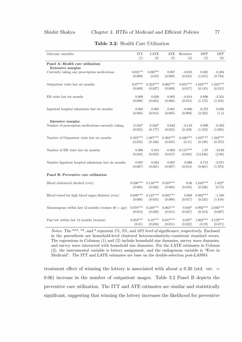
Shishir Shakya Chapter 3. HTEs of Medicaid and Efficient Policies 77
Table 3.2: Health Care Utilization
Outcome variables ITT LATE ATE Heuristic MFP DFP(1) (2) (3) (4) (5) (6)
Panel A: Health care utilizationExtensive margins
Currently taking any prescription medications 0.021** 0.067** 0.007 -0.018 0.801 -0.494(0.009) (0.03) (0.009) (0.018) (1.015) (0.734)
Outpatient visits last six months 0.07*** 0.224*** 0.062*** 0.055*** 1.028*** 1.316***(0.009) (0.027) (0.009) (0.017) (0.145) (0.312)
ER visits last six months 0.009 0.029 0.005 -0.014 0.696 -3.331(0.008) (0.024) (0.008) (0.015) (1.172) (1.816)
Inpatient hospital admissions last six months 0.002 0.005 0.001 -0.006 0.272 -0.626(0.004) (0.014) (0.005) (0.009) (2.322) (1.4)
Intensive marginsNumber of prescription medications currently taking 0.104* 0.342* 0.042 -0.119 0.899 -0.383
(0.055) (0.177) (0.055) (0.109) (1.219) (1.005)
Number of Outpatient visits last six months 0.335*** 1.087*** 0.304*** 0.426*** 1.037*** 1.502***(0.052) (0.166) (0.055) (0.11) (0.188) (0.373)
Number of ER visits last six months 0.006 0.018 -0.003 -0.115*** 1.97 -10.89(0.016) (0.053) (0.017) (0.035) (14.846) (2.98)
Number Inpatient hospital admissions last six months 0.007 0.024 0.007 0.008 0.713 -2.071(0.007) (0.021) (0.007) (0.014) (0.661) (1.974)
Panel B: Preventive care utilization
Blood cholesterol checked (ever) 0.036*** 0.116*** 0.035*** 0.00 1.043*** 1.022*(0.008) (0.026) (0.008) (0.016) (0.236) (0.73)
Blood tested for high blood sugar/diabetes (ever) 0.038*** 0.121*** 0.035*** 0.003 0.982*** -1.588(0.008) (0.025) (0.008) (0.017) (0.235) (1.618)
Mammogram within last 12 months (women 40 + age) 0.078*** 0.249*** 0.063*** 0.048* 0.992*** 2.036***(0.013) (0.039) (0.014) (0.027) (0.213) (0.697)
Pap test within last 12 months (women) 0.053*** 0.18*** 0.047*** 0.037* 1.003*** 2.159***(0.01) (0.034) (0.011) (0.022) (0.23) (0.671)
Notes: The ***, **, and * represent 1%, 5%, and 10% level of significance, respectively. Enclosedin the parenthesis are household-level clustered heteroscedasticity-consistent standard errors.The regressions in Columns (1) and (2) include household size dummies, survey wave dummies,and survey wave interacted with household size dummies. For the LATE estimates in Column(2), the instrumental variable is lottery assignment, and the endogenous variable is “Ever inMedicaid”. The ITT and LATE estimates are base on the double-selection post-LASSO.
treatment effect of winning the lottery is associated with about a 0.30 (std. err. =
0.06) increase in the number of outpatient usages. Table 3.2 Panel B depicts the
preventive care utilization. The ITT and ATE estimates are similar and statistically
significant, suggesting that winning the lottery increases the likelihood for preventive

Shishir Shakya Chapter 3. HTEs of Medicaid and Efficient Policies 78
cares like a blood test for cholesterol and diabetes, mammograms (for women of age
40+), or Pap tests (for women). However, these estimates are small in size and also
do not shed light on the treatment heterogeneity. There is likely no effect among a
particular subgroup, while another subgroup may be uniquely affected.
Table 3.2 Column (4) renders the heuristic approach to test the treatment het-
erogeneity. Evidence of treatment heterogeneity for outpatient usages and preventive
care utilization is found. Table 3.2 Column (5) shows the MFP and Column (6)
represents the DFP. The MFP and DFP are close to unit and statistically nonzero,
suggesting treatment heterogeneity among these variables.
Note that 2000 causal trees were assembled to develop a cluster-robust random
forest. Among these 2000 causal trees, the algorithm always selects the age and the
household income below the federal poverty level along with the household size and
other variables like education and employment. Appendix A provides the variable
importance table for all of the outcomes analyzed. It lists the variables which were
split (more than average) by the random forest. Only for illustration purpose of
treatment heterogeneity, I develop a heatmap by grouping age and percentage of
household income below the FPL and average the out-of-bag conditional average
treatment. The heatmap has age on the x−axis and Household Income below the
FPL (in percentage) on the y−axis.
Figure 3.2 Panel (a) to (e) renders graphical depictions that compare the treatment
and control group to exhibit the treatment heterogeneity for the outpatient usages
and preventive care. Figure 3.2 Panel (a) and (b) portray an insight into outpatient
utilization, CATE, over Age and household income. It appears that outpatient usage
CATE (in extensive margin) for lottery winners is high and positive for those who
belong to a household whose income lies below 100% of the FPL, regardless of age
cohorts. The findings are similar for the intensive margin of outpatient usage CATE;
however, there exist some additional heterogeneity for different age-cohorts.
Figure 3.2 Panel (c) exhibits treatment heterogeneity if the blood test for choles-
terol level were ever done within the study period. Mostly younger age cohorts,

Shishir Shakya Chapter 3. HTEs of Medicaid and Efficient Policies 79
Figure 3.2: Health Care and Preventive Care Utilization
(a) Outpatient visits lastsix months
(b) Number of outpatientvisits last six months
(c) Blood cholesterolchecked (ever)
(d) Blood tested forhigh blood sugar/diabetes(ever)
(e) Mammogram withinlast 12 months (women40+)
(f) Pap test within last 12months (women)
Notes: The heatmap helps to exhibit which subpopulations are more or less susceptible to Med-icaid. For each heatmap, age is in the x-axis and household income as a percentage of the FPLis in the y-axis. For each grid of x-axis and y-axis, the color maps the intensity of individ-ualized treatment effect. However, a heatmap is a partial representation of overall treatmentheterogeneity and requires caution to interpret. Indeed there may exist several variables whichshould be taken into consideration for proper interpretation of heterogeneous treatment effect.Appendix B provides relevant variables list to explain each of the heatmaps in this section.
between 20 to 40, who belong to a more impoverished household, have a higher like-
lihood of this preventive test. Figure 3.2 Panel (e) shows the treatment subgroup
who are in a household below 80% of the FPL are more likely to the blood test for
diabetes. Figure 3.2 Panel (e) and (f) illuminates CATE for the Mammogram test
(for women whose age is above 40) and the Pap test (for women). It appears that
women aged 40 years and above who belong below 50% of the FPL households are
highly likely to elect to have a Mammogram test performed. Post 50 years, women
are likely to have a Mammogram test regardless of the household income is below the
FPL. The heatmap of the Pap test shows, women from households close to the FPL
or below 100% the FPL are likely to participate for the Pap test.

Shishir Shakya Chapter 3. HTEs of Medicaid and Efficient Policies 80
Financial Strain
Table 3.3 displays extensive margins and intensive margins of financial strains.
Winning the insurance lottery is associated with lower financial strains both in ex-
tensive and intensive margins. The ITT and ATE estimates for financial strains in
intensive margins quantify the results in dollar terms as the net effect of winning
the lottery. The ITT and ATE ranges describe that winning the lottery relates to
reductions of various types of out-of-pocket costs for the past six months. The ITT
and ATE estimate ranges depicts on average $20 reductions on out-of-pocket costs for
doctors visits, clinics or health centers; nearly $40 to $49 reduction on out-of-pocket
costs for emergency room or overnight hospital care; about $13 to $15 reduction
on out-of-pocket costs for medical care and nearly about $50 reduction on the total
out-of-pocket cost for medical care. Other than these financial strains, the group
that received insurance through the lottery also has nearly $450 to $500 on average
reduction of their medical debts.
The “best linear prediction” (BPL) model narrates the treatment heterogeneity
in the out-of-pocket expenses (last six months) only. Again, this does not necessarily
mean that there is no heterogeneity because the BPL acts as an omnibus test for
the presence of heterogeneity. A closer look at the heatmap in Figure 3.3 illuminates
some sources of treatment heterogeneity.
The heatmap of Figure 3.3 Panel (a) shows a reduction for the extensive mar-
gin on the out-of-pocket medical expenses (last 6 months) suggesting lower financial
strain for lottery winners of all age groups and all households but the effects are more
pronounced for lottery winning households with income that ranges below 80% the
FPL and belong to the age group of 40 years and above. Figure 3.3 Panel (b) ex-
hibits a sharp discontinuity of owing money for medical expenses for lottery winning
households with income below 100% the FPL. These differences suggest that at least
within a low-income and relatively older population, individuals who select health
insurance coverage are in poorer health (and therefore demand more medical care)
than those who are uninsured, just as standard adverse selection theory would predict

Shishir Shakya Chapter 3. HTEs of Medicaid and Efficient Policies 81
Table 3.3: Financial Strain
Outcome variables ITT LATE ATE Heuristic MFP DFP(1) (2) (3) (4) (5) (6)
Extensive margins
Any out-of-pocket medical -0.073*** -0.238*** -0.073*** 0.028 1.021*** 1.449***expenses, last six months (0.009) (0.029) (0.009) (0.018) (0.125) (0.562)
Owe money for medical -0.053*** -0.17*** -0.058*** 0.038** 1.076*** 0.87expenses currently (0.009) (0.027) (0.009) (0.018) (0.169) (1.253)
Borrowed money or skipped other -0.057*** -0.184*** -0.064*** 0.008 1.061*** 0.473bills to pay medical bills, last six months (0.009) (0.028) (0.009) (0.017) (0.145) (1.323)
Refused treatment because of -0.012** -0.037** -0.013*** 0.006 1.054*** -3.706medical debt, last six months (0.005) (0.015) (0.005) (0.009) (0.387) (2.121)
Intensive margins
out-of-pocket costs for doctors visits, -19.308*** -61.429*** -20.175*** -8.47 0.999*** 0.371clinics or health centers, past 6 months (3.46) (10.919) (3.594) (7.192) (0.179) (0.664)
out-of-pocket costs for emergency room -49.519** -157.71** -40.73** 14.213 1.035** 0.211or overnight hospital care, past 6 months (21.611) (67.674) (18.46) (36.89) (0.468) (0.689)
out-of-pocket costs for prescription -15.042** -45.756** -12.747** 2.234 0.889** -1.116medicine, past 6 months (6.941) (22.054) (6.012) (12.067) (0.403) (1.405)
out-of-pocket costs for other -3.431 -10.577 -3.052 -7.223* 0.894* -3.693medical care, past 6 months (2.088) (6.55) (2.083) (4.188) (0.617) (1.492)
Total out-of-pocket costs for -48.203*** -152.815*** -53.793*** 13.3 1.034*** 0.489medical care, last 6 months (9.552) (30.393) (9.751) (19.707) (0.188) (0.732)
Total amount currently owed -442.39*** -1447.906*** -496.084*** 167.277 1.038*** -0.298for medical expenses (96.744) (318.1) (105.023) (208.674) (0.223) (1.125)
Notes: The ***, **, and * represent 1%, 5%, and 10% level of significance, respectively. Enclosedin the parenthesis are household-level clustered heteroscedasticity-consistent standard errors.The regressions in Columns (1) and (2) include household size dummies, survey wave dummies,and survey wave interacted with household size dummies. For the LATE estimates in Column(2), the instrumental variable is lottery assignment, and the endogenous variable is “Ever inMedicaid”. The ITT and LATE estimates are base on the double-selection post-LASSO.
Finkelstein et al. (2012).
Figure 3.3 Panel (c) shows no heterogeneity of being refused for treatment because
of medical debt. Privately-owned hospitals may refuse patients in a non-emergency,
but public hospitals cannot turn away patients. The Emergency Medical and Treat-
ment Labor Act (EMTLA) enacted by Congress in 1986, explicitly prohibits public
hospitals from denying care to indigent or uninsured patients even if they cannot pay.
Figure 3.3 Panel (d) shows that lottery winners have an overall reduction of bor-

Shishir Shakya Chapter 3. HTEs of Medicaid and Efficient Policies 82
Figure 3.3: Financial Strain
(a) Any out-of-pocketmedical expenses, last 6months
(b) Owe money for medi-cal expenses currently
(c) Refused treatment be-cause of medical debt, lastsix months
(d) Borrowed money orskipped other bills topay medical bills, last 6months
(e) out-of-pocket costs fordoctors visits, clinics orhealth centers, past 6months
(f) out-of-pocket costsfor emergency room orovernight hospital care,past 6 months
(g) out-of-pocket costsfor prescription medicine,past 6 months
(h) Total out-of-pocketcosts for medical care, last6 months
(i) Total amount cur-rently owed for medicalexpenses
Notes: The heatmap helps to exhibit which subpopulations are more or less susceptible to Med-icaid. For each heatmap, age is on the x-axis, and household income as a percentage of the FPLis on the y-axis. For each grid of the x-axis and y-axis, the color maps the intensity of the indi-vidualized treatment effect. However, a heatmap is a partial representation of overall treatmentheterogeneity and requires caution to interpret. Indeed there may exist several variables thatshould be taken into consideration for proper interpretation of heterogeneous treatment effect.Appendix B provides a relevant variables list to explain each of the heatmaps in this section.
rowing money or skipping other bills to pay medical costs compared to the control
group. However, the effect is more pronounced for lottery winning households with

Shishir Shakya Chapter 3. HTEs of Medicaid and Efficient Policies 83
income below 100% of the FPL compared to a similar control group. These estimates
are for the extensive margin only. The next figure exhibits some of the intensive
margins of financial strains.
Figure 3.3 Panel (e) shows that more than $25 to $30 reductions of out-of-pocket
costs (for doctors visits, clinics or health centers in past six months) for age group
50 plus who belongs to the lottery winning household with an income below 80% of
the FPL compared to the control group. The below 40 age group from the lottery
winning households within the range of 80% to 200% of the FPL have less than about
$15 reductions of such cost compared to the similar control group. The rest of the
lottery winning subgroup has roughly an average of $20 cuts of such cost, compared
to the control group.
Figure 3.3 Panel (f) shows about $60 to $70 or more reduction in the out-of-pocket
costs for emergency room or overnight hospital care in the past six months for the
age group of 40 below of the lottery winning household with income below 100%
of the FPL. The reduction of such costs is less than $20 for the 50 and above age
group, regardless of their household-level income status. The remaining subgroup of
these aged below 50 who belong to a household with income more than 100% of the
FPL has about $30 to $50 reductions in the costs of the out-of-pocket payments for
emergency room visits or overnight hospital stays.
Figure 3.3 Panel (g) exhibits that the lottery winners who belong to the household
with income below 100% the FPL (regardless of their age) report more than $15 of
reductions in the out-of-pocket costs for prescription medicine in past six months.
Figure 3.3 Panel (h) illuminates that the lottery winners who belong to a house-
hold with income below 100% the FPL (regardless of their age) have more than $50
of reductions in the total out-of-pocket cost for medical care in last six months.
Figure 3.3 Panel (i) exhibits the decline of the total amount currently owed for
medical expenses. Compared to the control group, the treatment group with the age
of 35 to 50, have medical debt reductions. Such medical debt reductions are more
pronounced (more than $600) if the person belongs to a household with an income of
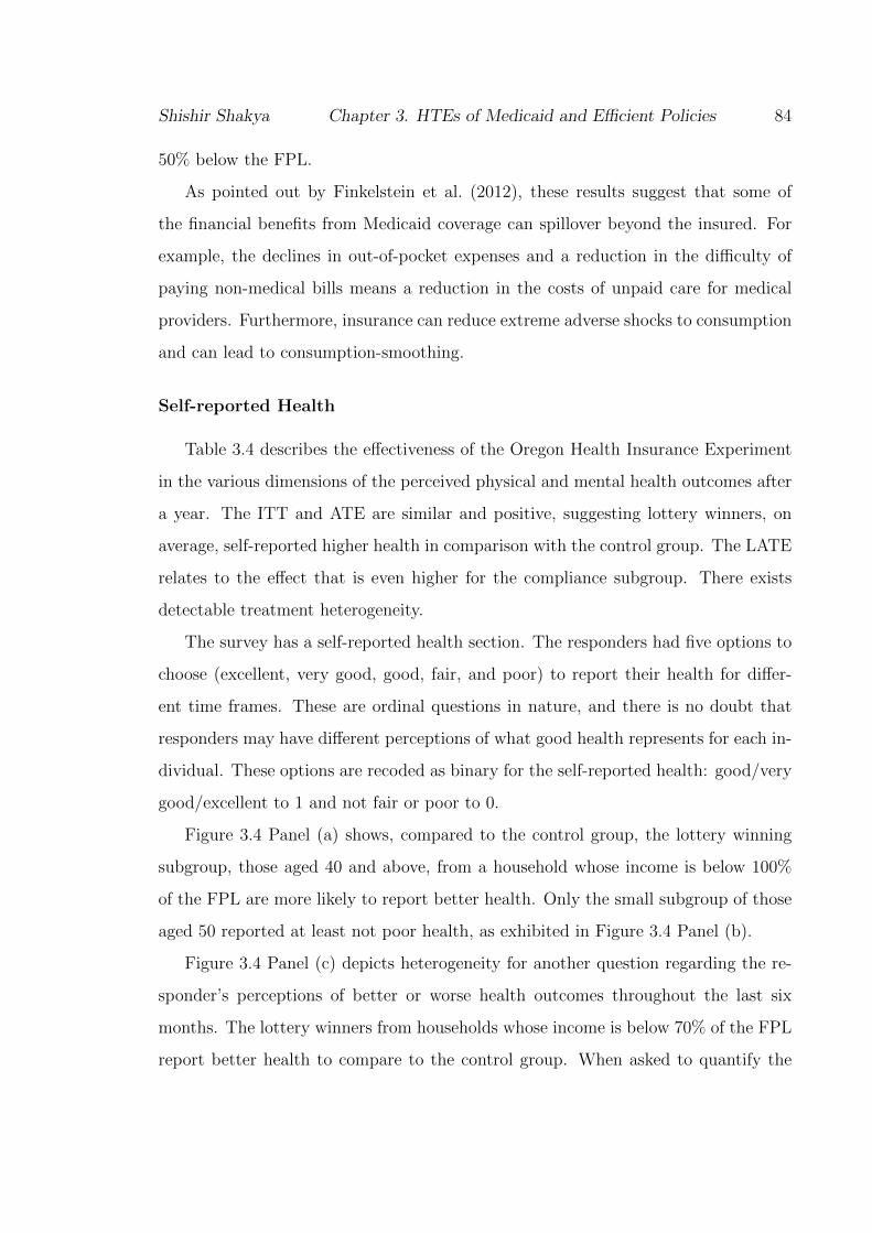
Shishir Shakya Chapter 3. HTEs of Medicaid and Efficient Policies 84
50% below the FPL.
As pointed out by Finkelstein et al. (2012), these results suggest that some of
the financial benefits from Medicaid coverage can spillover beyond the insured. For
example, the declines in out-of-pocket expenses and a reduction in the difficulty of
paying non-medical bills means a reduction in the costs of unpaid care for medical
providers. Furthermore, insurance can reduce extreme adverse shocks to consumption
and can lead to consumption-smoothing.
Self-reported Health
Table 3.4 describes the effectiveness of the Oregon Health Insurance Experiment
in the various dimensions of the perceived physical and mental health outcomes after
a year. The ITT and ATE are similar and positive, suggesting lottery winners, on
average, self-reported higher health in comparison with the control group. The LATE
relates to the effect that is even higher for the compliance subgroup. There exists
detectable treatment heterogeneity.
The survey has a self-reported health section. The responders had five options to
choose (excellent, very good, good, fair, and poor) to report their health for differ-
ent time frames. These are ordinal questions in nature, and there is no doubt that
responders may have different perceptions of what good health represents for each in-
dividual. These options are recoded as binary for the self-reported health: good/very
good/excellent to 1 and not fair or poor to 0.
Figure 3.4 Panel (a) shows, compared to the control group, the lottery winning
subgroup, those aged 40 and above, from a household whose income is below 100%
of the FPL are more likely to report better health. Only the small subgroup of those
aged 50 reported at least not poor health, as exhibited in Figure 3.4 Panel (b).
Figure 3.4 Panel (c) depicts heterogeneity for another question regarding the re-
sponder’s perceptions of better or worse health outcomes throughout the last six
months. The lottery winners from households whose income is below 70% of the FPL
report better health to compare to the control group. When asked to quantify the

Shishir Shakya Chapter 3. HTEs of Medicaid and Efficient Policies 85
Table 3.4: Self-reported Health
Variables ITT LATE ATE Heuristic MFP DFP(1) (2) (3) (4) (5) (6)
Self-reported health good/very 0.046*** 0.15*** 0.046*** 0.032* 0.984*** 1.485***good/excellent (not fair or poor) (0.009) (0.028) (0.009) (0.017) (0.19) (0.431)
Self-reported health not 0.033*** 0.107*** 0.033*** 0.044*** 1.036*** 1.085***poor (fair, good, very good, or excellent) (0.006) (0.019) (0.006) (0.012) (0.188) (0.316)
Health about the same or gotten 0.035*** 0.115*** 0.039*** 0.078*** 1.086*** 1.748***better over last six months (0.008) (0.026) (0.008) (0.016) (0.223) (0.437)
Number of days physical 0.557*** 1.796*** 0.602*** 0.431 1.037*** 1.011***health good, past 30 days (0.182) (0.587) (0.183) (0.364) (0.312) (0.4)
Number days poor physical or mental 0.432** 1.397** 0.454** 1.333*** 1.157** 1.286***health did not impair usual activity, past 30 days (0.198) (0.641) (0.197) (0.392) (0.511) (0.421)
Number of days mental health 0.741*** 2.479*** 0.806*** 0.807** 1.041*** 0.815***good, past 30 days (0.209) (0.675) (0.207) (0.411) (0.27) (0.311)
Did not screen positive for 0.024*** 0.079*** 0.027*** 0.023 1.055*** 0.657depression, last two weeks (0.008) (0.027) (0.008) (0.017) (0.338) (0.81)
Notes: The ***, **, and * represent 1%, 5%, and 10% level of significance, respectively. Enclosedin the parenthesis are household-level clustered heteroscedasticity-consistent standard errors.The regressions in Columns (1) and (2) include household size dummies, survey wave dummies,and survey wave interacted with household size dummies. For the LATE estimates in Column(2), the instrumental variable is lottery assignment, and the endogenous variable is “Ever inMedicaid”. The ITT and LATE estimates are base on the double-selection post-LASSO.
number of good physical health days in the past 30 days, lottery winning households
closer to the FPL report higher numbers, as presented in Figure 3.4 Panel (d).
However, in Figure 3.4 Panel (e), the number of good mental health days in the
past 30 days is reported to be higher for the age group above 40 from the lottery
winning households closer to the FPL. The severity of mental and physical health is
captured from the question to quantify the number of poor physical or mental health
days did not impair the usual activity, past 30 days. Again, households closer to
the FPL report higher numbers of days that were not impaired by poor physical and
mental health, as plotted in Figure 3.4 Panel (f).
Figure 3.4 Panel (g) shows a group of those aged 50 and above who are from a
household below 100% of the FPL are more likely to not be among those detected with
depression (in the last two weeks). In all these Panels, it is repeatedly observed that
lottery winning, poorer households report slightly better health outcomes compared

Shishir Shakya Chapter 3. HTEs of Medicaid and Efficient Policies 86
Figure 3.4: Self-reported Health
(a) Self-reported healthgood/very good/excellent(not fair or poor)
(b) Self-reported healthnot poor (fair, good, verygood, or excellent)
(c) Health about the sameor gotten better over lastsix months
(d) Number of days phys-ical health good, past 30days
(e) Number of days men-tal health good, past 30days
(f) Number days poorphysical or mental healthdid not impair usual activ-ity, past 30 days
(g) Did not screen pos-itive for depression, lasttwo weeks
Notes: The heatmap helps to exhibit which subpopulations are more or less susceptible to Med-icaid. For each heatmap, age is on the x-axis, and household income as a percentage of the FPLis on the y-axis. For each grid of the x-axis and y-axis, the color maps the intensity of the indi-vidualized treatment effect. However, a heatmap is a partial representation of overall treatmentheterogeneity and requires caution to interpret. Indeed there may exist several variables thatshould be taken into consideration for proper interpretation of heterogeneous treatment effect.Appendix B provides a relevant variables list to explain each of the heatmaps in this section.
to those who were not selected in the lottery. These results could arise due to adverse
selection. As the theory suggests, those who are typically viewed as poorer/older

Shishir Shakya Chapter 3. HTEs of Medicaid and Efficient Policies 87
require more health services than their counterparts. When they can receive that
care, they will report better health outcomes compared to the groups that are unable
to acquire that care.
Potential Mechanism for Improved Health
Table 3.5 depicts some potential mechanisms by which health insurance could
have improved objective physical health along the heterogeneities in these mecha-
nisms. Table 3.5 Columns (1), (2), and (3) present statistically significant increases
of self-reported access to care (Panel A), quality of care (Panel B), and happiness
(Panel C). Overall, the evidence suggests that people feel better off due to insurance,
but Finkelstein et al. (2012) point-out that with the current data, it is difficult to de-
termine the fundamental drivers of this improvement. One way to look at the drivers
of this improvement is to capture the treatment heterogeneities. Except for the use
of ER for a non-emergence (last six months), there are treatment heterogeneities in
the access to care, quality of care, and happiness detailed in Table 3.5 Columns (4),
(5), and (6).
Figure 3.4 illustrates the heatmap with age in the x−axis and percentage of house-
hold income below the FPL in the y−axis. The treatment effects are plotted for every
possible grid of age and percentage of household income below the FPL. Figure 3.4
Panel (a) exhibits a particular threshold that households with income below the FPL
90% are more likely to have the usual place of clinic-based care than the control
subgroup of similar attributes.
Figure 3.4 Panel (b) depicts households with income above 100% of the FPL with
those aged 40 years and above are less likely to have a personal doctor compared
to the households with income below 100% of the FPL with those aged under 40.
Most of the poorer households are likely to get all their needed medical care (Figure
3.4 Panel (c)) and medications (Figure 3.4 Panel (d)) while households with income
below 50% of the FPL and aged 40 age and above are less likely to utilize the ER in
instance of non-emergencies (Figure 3.4 Panel (e)). Perceived quality of care is very

Shishir Shakya Chapter 3. HTEs of Medicaid and Efficient Policies 88
Table 3.5: Potential Mechanism for Improved Health
Variables ITT LATE ATE Heuristic MFP DFP(1) (2) (3) (4) (5) (6)
Panel A: Access to careHave usual place 0.087*** 0.274*** 0.086*** 0.041** 1.012*** 2.185***
of clinic-based care (0.009) (0.029) (0.009) (0.018) (0.109) (0.736)
Have personal doctor 0.073*** 0.235*** 0.072*** 0.101*** 1.031*** 1.329***(0.009) (0.029) (0.009) (0.018) (0.127) (0.202)
Got all needed medical 0.085*** 0.274*** 0.085*** 0.095*** 1.019*** 1.985***(0.009) (0.028) (0.009) (0.017) (0.106) (0.332)
Got all needed drugs, 0.07*** 0.227*** 0.073*** 0.058*** 1.016*** 1.733***last six months (0.008) (0.026) (0.008) (0.016) (0.112) (0.416)
Didn’t use ER for 0.00 0.00 0.003 -0.04*** 1.163 -4.168non emergency, last six months (0.005) (0.015) (0.005) (0.01) (1.469) (2.29)
Panel B: Quality of careQuality of care received last six months 0.049*** 0.15*** 0.053*** -0.312*** 1.028*** -402.796
good/very good/excellent (conditional on any) (0.01) (0.03) (0.01) (0.019) (0.179) (19.252)
Panel C: HappinessHappiness, very happy or pretty 0.062*** 0.202*** 0.069*** 0.057*** 1.049*** 1.551***
happy (vs. not too happy) (0.009) (0.029) (0.009) (0.017) (0.134) (0.379)
Notes: The ***, **, and * represent 1%, 5%, and 10% level of significance, respectively. Enclosedin the parenthesis are household-level clustered heteroscedasticity-consistent standard errors.The regressions in Columns (1) and (2) include household size dummies, survey wave dummies,and survey wave interacted with household size dummies. For the LATE estimates in Column(2), the instrumental variable is lottery assignment, and the endogenous variable is “Ever inMedicaid”. The ITT and LATE estimates are base on the double-selection post-LASSO.
uniformly distributed among the households and all age groups (Figure 3.4 Panel (f)).
However, aged 40 and above in households with income below 180% of the FPL are
more likely to have perceived happiness (Figure 3.4 Panel (d)).
3.5.3 Efficient Policies
The previous section describes the ITT, LATE, and ATE along with the test of
treatment heterogeneity. A more interesting question is whether we can find ways
to prioritize treatment to some subgroups of Medicaid eligible registrants who are
more likely to benefit from it. Following the out-of-bag prediction using generalized
random forests of the Athey and Wager (2019b), I compute doubly-robust scores for
the treatment effect as in equation 3.8, and learning policies empirical maximization

Shishir Shakya Chapter 3. HTEs of Medicaid and Efficient Policies 89
Figure 3.5: Potential Mechanism for Improved Health
(a) Have usual place ofclinic-based care (b) Have personal doctor
(c) Got all needed medicalcare, last six months
(d) Got all needed drugs,last six months
(e) Didn’t use ER for non-emergency, last six months
(f) Quality of care re-ceived last six monthsgood/very good/excellent(conditional on any)
(g) Happiness, very happyor pretty happy (vs. nottoo happy)
Notes: The heatmap helps to exhibit which subpopulations are more or less susceptible to Med-icaid. For each heatmap, age is on the x-axis, and household income as a percentage of the FPLis on the y-axis. For each grid of the x-axis and y-axis, the color maps the intensity of the indi-vidualized treatment effect. However, a heatmap is a partial representation of overall treatmentheterogeneity and requires caution to interpret. Indeed there may exist several variables thatshould be taken into consideration for proper interpretation of heterogeneous treatment effect.Appendix B provides a relevant variables list to explain each of the heatmaps in this section.
as in equation 3.9.
Table 3.6 Column (1) details the average outcome for each policy variable of inter-
est under the random assignment of treatment. Table 3.6 Columns (2) to (5) present

Shishir Shakya Chapter 3. HTEs of Medicaid and Efficient Policies 90
Table 3.6: Estimate of the Utility Improvement of Various Policies Over Baseline.
Variable Baseline Probability rule CATE rule Shallow tree Deeper tree(1) (2) (3) (4) (5)
Panel A: Health care utilizationOutpatient visits 0.604*** 4.74*** 5.119*** 4.228*** 2.898***
last six months (0.002) (0.182) (0.17) (0.197) (0.177)
Panel B: Preventive care utilizationBlood cholesterol checked (ever) 0.659*** 0.575*** 3.023*** 1.934*** 1.59***
(0.005) (0.176) (0.146) (0.166) (0.154)
Blood tested for high blood 0.625*** 1.066*** 3.059*** 2.665*** 2.068***sugar/diabetes (ever) (0.003) (0.157) (0.124) (0.137) (0.178)
Mammogram within last 0.331*** 7.008*** 10.228*** 9.26*** 5.75***12 months (women + 40) (0.002) (0.482) (0.398) (0.552) (0.42)
Pap test within last 0.411*** 3.489*** 5.682*** 4.955*** 4.058***12 months (women) (0.003) (0.286) (0.24) (0.315) (0.316)
Panel C: Self-reported healthSelf-reported health good/very 0.579*** 1.952*** 4.186*** 4.225*** 2.588***
good/excellent (not fair or poor) (0.003) (0.174) (0.145) (0.201) (0.195)
Panel D: Potential mechanismHave usual place 0.558*** 5.462*** 7.44*** 7.305*** 4.718***
of clinic-based care (0.002) (0.227) (0.203) (0.237) (0.202)
Have personal doctor 0.544*** 6.114*** 6.432*** 6.144*** 4.576***(0.003) (0.192) (0.207) (0.244) (0.181)
Happiness, very happy or pretty 0.629*** 2.137*** 4.883*** 5.042*** 3.306***happy (vs. not too happy) (0.002) (0.196) (0.174) (0.218) (0.166)
Notes: The ***, **, and * represent 1%, 5%, and 10% level of significance, respectively. Enclosedin the parenthesis are standard errors. The estimates in Columns (1) represents the averages ofeach variable based on the random assignment baseline and considered as a parameter measuringthe cost of treatment. The estimates in Column (2) to (5) presents the estimates of the averageoutcome improvement (in percentage) of various policies over a random assignment baseline forselected variable of interest. Policies learned on different subsets of the data will in general bedifferent from the policies learned on the full data. Therefore, to examine the stability of thelearned rule, 100 different policy are learned from randomly sample subdata and estimates arebased on the out-of-bag sample.
the estimates of the average outcome improvement (in percentage) of various policies
over a random assignment baseline for the selected variable of interest. Efficient pol-
icy for each of the variables of interest uses a particular set of covariates, as given in
appendix B. However, I did not use covariates like gender and race for the ethical
and political rationale because these covariates cannot legally be used for treatment
allocation.
In Table 3.6 Column (2) the assignment policy is based on a probability rule. The

Shishir Shakya Chapter 3. HTEs of Medicaid and Efficient Policies 91
Figure 3.6: Efficient Policy to Improve Outpatient Visits
(a) Shallow tree (b) Deep tree
Notes: The hhinc pctthe FPL 0m shows household income as percentage of the federal povertyline in the baseline and the ins months 0m num shows numbers of months that a responder hasinsurance in last six months. Policies learned on different subsets of the data will in general bedifferent from the policies learned on the full data, and it can be interesting to examine them togain intuition for the stability of the learned rule. Table 3.6 exhibits the stability of learned rule,however, Figure 3.6 is a graphical depiction of a learned policy and can be different to differentsubsets of the data.
probability rule allocates Medicaid for those whose probability is less than the aver-
age probability of each outcome of interest. The generalized random forest provides
the probability for each outcome of interest. In Table 3.6 Column (3), the assign-
ment policy is the CATE rule, i.e., assign Medicaid if CATE is positive. In Table
3.6 Columns (4) and (5), the shallow and deeper causal tree provides the Medicaid
assignment policies. The shallow causal tree allows a max-depth of 3 policy trees
while the deeper causal tree allows the max-depth of policy tree to be obtained by
optimal pruning of the causal tree using cross-validation. Caution is warranted as
asymptotic results hold only for trees with little complexity.
Table 3.6 Panel A, Column (1) describes the percentage of the households with
outpatient visits over the last six months using the full sample data. About 60% of the
whole sample has an outpatient visit in the previous six months. Note, this estimate is
based on the lottery assignment of the OHP Standard or Medicaid. Panel A, Column
(2) presents that if the Medicaid or OHP Standard is assigned among the eligible
registrants using the probability rule, then it would improve outpatient visits by an

Shishir Shakya Chapter 3. HTEs of Medicaid and Efficient Policies 92
additional 4.74%. Panel A, Column (3), exhibits, if the Medicaid assignment is based
on the CATE rule, then it would improve outpatient visits by 5.12%. The optimal
depth-3 policy tree or shallow tree would improve outpatient visits by an additional
4.23%. The optimal depth for policy trees based on the cross-validation for pruning
would improve outpatient visits by an extra 2.9%. All of these improvements are
statistically significant.
Figure 3.6 is a graphical depiction of the proposed efficient policy with the shallow
tree in Panel (a) and deep tree in Panel (b). Note that the policies learned on different
subsets of the data will, in general, be different from the policies acquired on the full
data. It can be interesting to examine them to gain an intuition for the stability of
the learned rule. Table 3.6 exhibits the stability of learned rule. However, Figure 3.6
is a graphical depiction of a learned policy and can vary for different subsets of the
data. To save space, learned efficient policies for the rest of the variables that are
presented in Table 3.6 are compiled in Appendix C.
3.6 Discussion and Conclusion
In 2008, 10,000 low-income Oregonian adults (19 to 64 years of age) were ran-
domly chosen to qualify for Medicaid, which provides a unique opportunity to study
the causal effect of Medicaid coverage. Finkelstein et al. (2012) found in the year
following the random assignment of Medicaid, the treatment group had higher health
care use, lower out-of-pocket medical expenditures and medical debt, and better self-
reported physical and mental health than the control group, but it did not have
detectable improvements in physical health conditions like high blood pressure. How-
ever, these mixed-bag effects of Medicaid puzzle researchers to determine what drives
the relationship between Medicaid and other outcomes of interest. My paper puts for-
ward an argument of heterogeneous treatment effect where Medicaid distinctly affects
different individuals and subpopulations differently. Furthermore, I use these hetero-
geneous treatment effects to reveal policy reforms. These reforms prioritize Medicaid

Shishir Shakya Chapter 3. HTEs of Medicaid and Efficient Policies 93
allotments to the subgroups that are likely to benefit the most. I also quantify how
much these reforms improve from the baseline Medicaid impacts on health care use,
personal finance, health, and well-being.
In this section, I present discussions on some of the obvious questions that the
reader may have. This paper contemplates a situation where analysts know their
outcome variable, (Y ), at the post-treatment and have data of observables, (X), at
the pre-treatment period. This situation may be a standard for many researchers. For
this reason, this paper analyzes the data as an observational rather than a genuinely
randomized study. Therefore, the unconfoundedness assumption to identify causal
effects is crucial for this paper.
This paper focuses on “intent-to-treat” rather than “local average treatment ef-
fects.” A local average treatment effect can be interpreted as the impact of Medicaid
among compliers while an intent-to-treat estimates the net impact of expanding access
to Medicaid. The results present both facts, but I mainly focus on the intent-to-treat
because the problem policymakers face only a choice of the eligibility criteria and
not the take-up. There can be many reasons for eligible people (lottery winner) not
to accept Medicaid and people who do not win the lottery to get other insurance
from other sources. This is the consumer’s sovereignty, and policymakers cannot
micromanage.
The heterogeneous effects of Medicaid are pronounced among households below
100% of the federal poverty line. A possible answer would be that more impoverished
families may need more medical care. Medicaid provides an opportunity for these
households to gain access to health care, and they, therefore, may utilize health care
more than those who are uninsured that can be an exemplification of a standard
adverse selection theory prediction. Also, I did not use the covariates like gender
and race for the ethical and political rationale because these covariates cannot legally
be used for treatment allocation. However, these are essential covariates, and not
including these covariates can lead to higher standard errors in the estimates.
The proposed policy can be thought of as small reforms in Medicaid. Rather than

Shishir Shakya Chapter 3. HTEs of Medicaid and Efficient Policies 94
a blanket policy that can be welfare-maximizing yet highly costly, these reforms target
the subpopulation who are more likely to derive benefit and because these reforms are
aimed, therefore, can be less expensive. For example, the federal government started
to defund Oregon’s Medicaid Expansion from 2016 which has led to a budget deficit
and Oregon Measure101 a two-year budget fix to close the state budget deficit by
taxing hospital and insurance agencies, is nearing to end in 2020, these proposed
reforms can help Oregon to reduce the state budget deficit.
To generalize the results outside the sample size, one needs to robustly account
for the sampling variability of potentially unexplained household-level effects. This
study takes a conservative approach and assumes that the outcome variables of an
individual within the same household may be arbitrarily correlated within a household
(or “cluster”), and therefore, utilizes the cluster-robust analysis. Each household is
equally weighted, such that the model allows the prediction of the effect on a new
individual from a new household, to generalize beyond the households given in the
data. However, caution must be taken. First, these estimates are the one-year impact
of expanding Medicaid access, and effects can change over longer time horizons than
we can analyze. Second, these findings are the partial equilibrium effects of covering a
small number of people, holding constant the rest of the health care system; the results
of much more extensive health insurance expansions might differ because of supply-
side responses by the health care sector. Third, the population is not representative of
the low-income uninsured adults in the rest of the United States on several observable
(and presumably unobservable) dimensions.
To conclude, I provide some evidence of heterogeneous treatment effects of Med-
icaid that can reconcile the mixed-bag results of Medicaid, as reported by previous
literature. I also proposed some reforms that can improve program effectiveness. The
Medicaid expansion, through the Affordable Care Act (ACA) and the contemporary
fiscal pressure, has triggered a national debate amongst diverse stakeholders regarding
the impacts of Medicaid coverage on various dimensions of public health, costs, and
benefits. Some have argued that Medicaid decreases total health care spending by
Shishir Shakya Chapter 3. HTEs of Medicaid and Efficient Policies 95
improving health and reducing inefficient hospital and emergency room utilization.
Others have disputed that Medicaid reneges the promised benefits because Medicaid
reimburses providers insufficiently, and therefore, recipients struggle to obtain access
to care, and the low income uninsured already have reasonable access to care through
clinics, uncompensated care, emergency departments, and out-of-pocket spending.
Both of these arguments eventually motivate a need for substantial discussion and
rigorous empirical assessment of what effects, if any, Medicaid coverage has on health
care, health, and well-being and how to strike a balance between cost and benefits.

96
Appendix A
Causal Machine Learning
Approaches
Average Treatment Effect In this paragraph, I show a few examples of a causal
machine learning approach to estimate the average treatment effect. For example,
Belloni et al. (2014b) and Belloni et al. (2014a) utilize “off-the-shelf” or readily avail-
able predictive machine learning algorithm called the “LASSO”1 method and purpose
a correction2 called the “double-selection post-LASSO”3 method. This method is use-
1The Least Absolute Shrinkage and Selection Operator (LASSO) is an appealing method to esti-mate the sparse parameter from a high-dimensional linear model is introduce by Frank and Friedman(1993) and Tibshirani (1996). The LASSO simultaneously performs model selection and coefficientestimation by minimizing the sum of squared residuals plus a penalty term. The penalty term pe-nalizes the size of the model through the sum of absolute values of coefficients. Consider a followinglinear model yi = Θiβ1 +εi, where Θ is high-dimensional covariates, the LASSO estimator is defined
as the solution to minβ1∈Rp
En
[(yi−iΘβ1)
2]
+ λn‖β1‖1, the penalty level λ is a tuning parameter to
regularize/controls the degree of penalization and to guard against over-fitting. The cross-validationtechnique chooses the best λ in prediction models and ‖β‖1 =
∑pj=1 |βj |. The kinked nature of
penalty function induces β to have many zeros; thus LASSO solution feasible for model selection.2When LASSO of outcome variable is implemented to select the covariates while always restricting
the treatment indicator, the estimated treatment effect is biased because LASSO’s sole objective isto select variables that predict outcome thus LASSO fails to select confounders that are also strongpredictor of treatment assignment.
3Belloni et al. (2014a) simplify the double-selection post-LASSO procedure as following. First,run LASSO of outcome variables on a large list of potential covariates to select a set of predictorsfor the outcome variable. Second, run LASSO of treatment variable on a large list of potentialcovariates to select a set of predictors for treatment. If the treatment is truly exogenous, we shouldexpect this second step should not select any variables. Third, run OLS regression of outcomevariable on treatment variable, and the union of the sets of regressors selected in the two LASSOruns to estimate the effect of treatment on the outcome variable then correct the inference with

APPENDIX A. CAUSAL MACHINE LEARNING APPROACHES 97
ful for estimating the average treatment effect when the analyst is required to select
a “sparse” outcome model4 from high-dimensional observables when some covariates
correlate with treatment and outcome, and the analyst does not know which ones
are important. Similarly, Athey et al. (2018) utilize “doubly-robust”5 method and
LASSO method and purpose “residual balancing”6 approach for estimating average
treatment effect under the assumption of unconfoundedness7 and the assumption of
the outcome model is linear and sparse. Similarly, Chernozhukov et al. (2018a) pur-
pose “double machine learning” for estimating the average treatment effect under
unconfoundedness. The idea is to first run any feasible machine learning methods
of outcomes on covariates, and then second run another feasible machine learning
methods of the treatment indicator on covariates; then, the residuals from the first
machine learning are regressed on the residuals from the second machine learning
to estimate the average treatment effect. This idea is similar to Frish-Waugh-Lovell
theorem8 and close to the concept of Robinson (1988) residual-on-residual regression
approaches where the estimator was a kernel regression. Heterogeneous Treatment
Effects Along with the average treatment effect, heterogeneous treatment effects es-
usual heteroscedasticity robust OLS standard error.4The “sparse” outcome model means a model with a few meaningful covariates that affect the
average outcome. These few meaningful covariates are selected from a given list of many observablescovariates, and potentially a situate when numbers of observables k are greater than numbers ofobservations n, i.e., k > n. When k > n, an estimation based on the least-squares estimation isinfeasible. However, traditionally, the principal component analysis (PCA) is commonly used toreduce dimension when the likelihood function is normal. The PCA creates principal componentsusing linear combinations of a much larger set of variables from a multivariate data-set. Interpretingthe coefficients on the principal components requires the researcher first to interpret the principalcomponents, which can prove a challenge as all variables have non-zero loadings.
5The “doubly-robust” estimator proceeds by taking the average of the efficient score, whichinvolves the estimation of conditional mean of outcomes given covariates as well as the inversepropensity score Athey (2018).
6The “residual balancing” replaces inverse propensity score weights with weights obtained usingquadratic programming, where the weights are designed to achieve balance between the treatmentand control group. The conditional mean of outcomes is estimated using LASSO Athey (2018).
7The unconfoundedness assumption implies treatment is randomly assigned and knowing ob-servable characteristics of an individual, and their treatment status gives no additional informationon the potential outcomes. This means the treatment assignment is independent of the outcomevariable.
8The Frisch-Waugh-Lovell theorem is that estimating a parameter in a multiple regression isequivalent to estimating the same parameter in a simple regression of the residual of the regress andregressed on all other predictors on the residual of the regressor regressed on all other predictors.

APPENDIX A. CAUSAL MACHINE LEARNING APPROACHES 98
timation interests policymakers because it helps to quantify the sizes of effects on
different subpopulations, which is valuable to improve program targeting and to un-
derstand the underlying mechanisms driving the results. Usually, data are stratified
in mutually exclusive groups or include interactions in a regression to explore het-
erogeneous treatment effects. However, ad-hoc searches for the responsive subgroups
may lead to false discoveries or may mistake noise for a true treatment effect (Davis
and Heller, 2017). Knaus et al. (2017) points out that for large-scale investigations
of effect heterogeneity, standard p−values of standard (single) hypothesis tests are
no longer valid because of the multiple hypothesis testing problems (Lan et al., 2016;
List et al., 2019) and leads to so-called “ex-post selection” problem which is widely
recognized in the program evaluation literature. For example, for fifty single hypothe-
ses tests, the probability that at least one test falsely rejects the null hypotheses at
the 5% significance level (assuming independent test statistics as an extreme case) is
1− 0.9550 = 0.92 or 92%.
The new avenue of causal machine learning provides a better systematic approach
to search the groups with heterogeneous treatment effects. One intuitive approach
proposed by Imai and Ratkovic (2013) is to sample-split and use the first sample to run
the LASSO regression model with the treatment indicator interacted with covariates
and perform variables selections then use the selected model with the second sample
to perform an ordinary least squares regression to guard against over-fitting. While
Athey and Imbens (2016) utilizes the Breiman et al. (1984) classification and regres-
sion tree (CART)9 machine learning algorithms and purpose “causal tree” method.
The CART recursively filters and partitions the large data-set into binary sub-groups
(nodes) such that the samples within each subset become more homogeneous that fit
the response variable. Unlike the CART that minimizes the mean-squared error of
the prediction of outcomes to capture heterogeneity in outcomes, the “causal” tree
9In simplest, the CART algorithm chooses a variable and split that variable above or below acertain level (which forms two mutually exclusive subgroups or leaves) such that the sum of squaredresiduals is minimized. This splitting process is repeated for each leave until the reduction in thesum of squared residuals is below a certain level as defined by users, thus resulting in a tree format(Athey and Imbens, 2017b).
APPENDIX A. CAUSAL MACHINE LEARNING APPROACHES 99
minimizes the mean-squared error of treatment effects to capture treatment effect
heterogeneity. The approach to estimate the “causal” tree is similar to Imai and
Ratkovic (2013) approach, in which half of the sample is used to determine the opti-
mal partition of covariates space, while the other half is used to estimate treatment
effects within the leave based on the optimal partition of covariates selected from the
first partition (Athey and Imbens, 2016). The sample-splitting approach also known
as “honest” estimation lead to loss of precision as only half of the data is used to
estimate the effect, but generates a treatment effect and a confidence interval for
each subgroup that is valid no matter how many covariates are used in estimation.
Athey and Imbens (2017b) points out that the researcher is free to estimate a more
complex model in the second part of the data, for example, if the researcher wishes to
include fixed effects in the model, or model different types of correlation in the error
structure.
The causal tree doesn’t provide personalized estimates, Wager and Athey (2018)
utilize the “random forest” machine learning approach and propose a “causal for-
est” method, where many different causal trees are generated and averaged. This
method provides causal effects that change more smoothly with covariates and pro-
vides distinct individualized estimates and confidence intervals. Wager and Athey
(2018) also shows that the predictions from causal forests are asymptotically normal
and centered on the true conditional average treatment effect for each individual.
Athey et al. (2016) extend the approach to other models for causal effects, such as
instrumental variables, or other models that can be estimated using the generalized
method of moments (GMM). In each case, the goal is to evaluate how a causal param-
eter of interest varies with covariates. Efficient Policy The optimal policy estimation
have received greater attention in the machine learning literature10 (Athey, 2018).
The optimal policy function map the observable characteristics of an individual to a
policy or treatment assignment. In simplest, the main goal of optimal policy estima-
10See Strehl et al. (2010); Dudık et al. (2011); Li et al. (2012); Dudık et al. (2014); Swaminathanand Joachims (2015); Jiang and Li (2015); Thomas and Brunskill (2016) and Kallus (2018).

APPENDIX A. CAUSAL MACHINE LEARNING APPROACHES 100
tion is to answer−- “who should be treated?” or optimal treatment allocation. The
understanding of optimal policy is essential in policymaking because an ad-hoc tar-
geting a specific subpopulation with positive interventions can be unfair, unethical,
illegal, and unpolitical to some other subpopulations while intervening everyone in
the population (a blanket policy) is welfare-maximizing but can be extremely costly.
The optimal policy estimation or optimal treatment allocation has been recently
studied in using causal machine learning in economics, mainly by Kitagawa and
Tetenov (2018) and Athey and Wager (2019a). The main idea is to select a pol-
icy function that minimizes the loss from failing to use the ideal policy, referred to as
the “regret” of the policy. Note that estimating conditional average treatment effect
or heterogeneous treatment effect focus on the squared-error loss while the optimal
policy estimation focuses on utilitarian regret Athey and Wager (2019a).

101
Appendix B
Variable Importance
Table B.1: Variable Importance
Variables FPL Age HHS INS Other variables
Currently taking any prescription medications X X X % MSAOutpatient visits last six months X X XER visits last six months X X XInpatient hospital admissions last six months X X X XNumber of prescription medications currently taking X X X XNumber of Outpatient visits last six months X X XNumber of ER visits last six months X X X X % High school disploma or GEDNumber Inpatient hospital admissions last six months X X X % Self signupAny out of pocket medical expenses, last six months X X X X % MSAOwe money for medical expenses currently X X XBorrowed money or skipped other bills to pay medical bills, last six months X X XRefused treatment because of medical debt, last six months X X XOut of pocket costs for doctors visits, clinics or health centers, past 6 months X X % work 30+ hrs/weekOut of pocket costs for emergency room or overnight hospital care, past 6 months X X XOut of pocket costs for prescription medicine, past 6 months X X X XOut of pocket costs for other medical care, past 6 months X X XTotal out of pocket costs for medical care, last 6 months X X X X % work 30+ hrs/weekTotal amount currently owed for medical expenses X X X XHave usual place of clinic-based care X XHave personal doctor X X X % work 30+ hrs/weekGot all needed medical care, last six months X X X X % work 30+ hrs/weekGot all needed drugs, last six months X X X % dont currently workDidn’t use ER for non emergency, last six months X X X % work 30+ hrs/weekQuality of care received last six months good/very good/excellent (conditional on any) X X X % MSAHappiness, very happy or pretty happy (vs. not too happy) X X X XBlood cholesterol checked (ever) X X X XBlood tested for high blood sugar/diabetes (ever) X X XMammogram within last 12 months (women 40) X X X X % work 30+ hrs/weekPap test within last 12 months (women) X X X % work 30+ hrs/weekSelf-reported health good/very good/excellent (not fair or poor) X X X XSelf-reported health not poor (fair, good, very good, or excellent) X X XHealth about the same or gotten better over last six months X X X % High school diploma or GEDNumber of days physical health good, past 30 days X X XNumber days poor physical or mental health did not impair usual activity, past 30 days X X X XNumber of days mental health good, past 30 days X X X X % FemaleDid not screen positive for depression, last two weeks X X X
Notes: FPL represents household below the federal poverty line (in %), HHS represents house-hold size, INS represents the nummber of non insurance months in last six months. The randomforest model always splits on FPL and Age along with HHS and INS. Along with these variablesthe random forest also splits on different variables included in the last column. For example,consider the model called “Currently taking any prescription medications”, the random forestsplits (more than average) the data on FPL, Age, HHS, and % MSA. Therefore, the treatmentheterogeneity is likely within these variables.

102
Appendix C
Efficient Policies
Figure C.1: Efficient Policy to Improve the Blood Cholesterol Check Participation
(a) Shallow tree (b) Deep tree
Notes: The hhinc pctfpl 0m shows household income as percentage of the federal poverty line.The ins months 0m num shows numbers of months that a responder has insurance in last sixmonths. The employ hrsmwork 30 hrs week shows > 0.5 shows the responder work more than30 hours per/week. The hhsize 0m is household size.

APPENDIX C. EFFICIENT POLICIES 103
Figure C.2: Efficient Policy to Improve Blood Tests Participation for High BloodSugar/Diabetes
(a) Shallow tree (b) Deep tree
Notes: The hhinc pctfpl 0m shows household income as percentage of the federal poverty line.The ins months 0m num shows numbers of months that a responder has insurance in last sixmonths. The employ hrsmwork 30 hrs week shows > 0.5 shows the responder work more than30 hours per/week. The hhsize 0m is household size.
Figure C.3: Efficient Policy to Improve Mammogram Test Participation for Women
(a) Shallow tree (b) Deep tree
Notes: The hhinc pctfpl 0m shows household income as percentage of the federal poverty line.The ins months 0m num shows numbers of months that a responder has insurance in last sixmonths. The employ hrsmwork 30 hrs week shows > 0.5 shows the responder work more than30 hours per/week. The hhsize 0m is household size. Valid only for women.

APPENDIX C. EFFICIENT POLICIES 104
Figure C.4: Efficient Policy to Improve Pap Test Participation for Women
(a) Shallow tree (b) Deep tree
Notes: The hhinc pctfpl 0m shows household income as percentage of the federal poverty line.The ins months 0m num shows numbers of months that a responder has insurance in last sixmonths. The employ hrsmwork 30 hrs week shows > 0.5 shows the responder work more than30 hours per/week. The hhsize 0m is household size. Valid only for women.
Figure C.5: Efficient Policy to Improve Self-reported Health
(a) Shallow tree (b) Deep tree
Notes: The hhinc pctfpl 0m shows household income as percentage of the federal poverty line.The ins months 0m num shows numbers of months that a responder has insurance in last sixmonths. The employ hrsmwork 30 hrs week shows > 0.5 shows the responder work more than30 hours per/week. The hhsize 0m is household size. Valid only for women.

APPENDIX C. EFFICIENT POLICIES 105
Figure C.6: Efficient Policy to Improve to have Usual Place of Clinic-based Care
(a) Shallow tree (b) Deep tree
Notes: The hhinc pctfpl 0m shows household income as percentage of the federal poverty line.The ins months 0m num shows numbers of months that a responder has insurance in last sixmonths. The employ hrsmwork 30 hrs week shows > 0.5 shows the responder work more than30 hours per/week. The hhsize 0m is household size. Valid only for women.
Figure C.7: Efficient Policy to Improve to have a Personal Doctor
(a) Shallow tree (b) Deep tree
Notes: The hhinc pctfpl 0m shows household income as percentage of the federal poverty line.The ins months 0m num shows numbers of months that a responder has insurance in last sixmonths. The employ hrsmwork 30 hrs week shows > 0.5 shows the responder work more than30 hours per/week. The hhsize 0m is household size. Valid only for women.

APPENDIX C. EFFICIENT POLICIES 106
Figure C.8: Efficient Policy to Improve to Post Health-care Service Happiness
(a) Shallow tree (b) Deep tree
Notes: The hhinc pctfpl 0m shows household income as percentage of the federal poverty line.The ins months 0m num shows numbers of months that a responder has insurance in last sixmonths. The employ hrsmwork 30 hrs week shows > 0.5 shows the responder work more than30 hours per/week. The hhsize 0m is household size. Valid only for women.

References 107
References
Abadie, A., Diamond, A., and Hainmueller, J. (2010). Synthetic Control Methods for
Comparative Case Studies: Estimating the Effect of California’s Tobacco Control
Program. Journal of the American Statistical Association, 105(490):493–505.
Abadie, A., Diamond, A., and Hainmueller, J. (2015). Comparative Politics and the
Synthetic Control Method. American Journal of Political Science, 59(2):495–510.
Abadie, A. and Gardeazabal, J. (2003). The economic costs of conflict: A case study
of the Basque country. American Economic Review.
Ali, M. M., Dowd, W. N., Classen, T., Mutter, R., and Novak, S. P. (2017). Prescrip-
tion drug monitoring programs, nonmedical use of prescription drugs, and heroin
use: Evidence from the national survey of drug use and health. Addictive Behaviors,
69:65 – 77.
Allen, H., Baicker, K., Finkelstein, A., Taubman, S., and Wright, B. J. (2010). What
the Oregon Health Study can Tell us about Expanding Medicaid. Health Affairs,
29(8):1498–1506.
Alpert, A., Powell, D., Liccardo Pacula, R., and Pacula, R. L. (2017). Supply-Side
Drug Policy in the Presence of Substitutes: Evidence from the introduction of
Abuse-Deterrent Opioids.
Angrist, J. and Pischke, J.-S. (2009). Mostly Harmless Econometrics: An Empiricist’s
Companion. Princeton University Press, 1 edition.
Athey, S. (2018). The Impact of Machine Learning on Economics. In The Economics
of Artificial Intelligence: An Agenda, number Ml, pages 1–27. University of Chicago
Press.
Athey, S. and Imbens, G. (2016). Recursive partitioning for heterogeneous causal
effects. Proceedings of the National Academy of Sciences, 113(27):7353–7360.

References 108
Athey, S. and Imbens, G. (2017a). Chapter 3 - the econometrics of randomized
experiments. In Banerjee, A. V. and Duflo, E., editors, Handbook of Field Ex-
periments, volume 1 of Handbook of Economic Field Experiments, pages 73 – 140.
North-Holland.
Athey, S. and Imbens, G. W. (2017b). The state of applied econometrics: Causality
and policy evaluation. Journal of Economic Perspectives, 31(2):3–32.
Athey, S., Imbens, G. W., and Wager, S. (2018). Approximate residual balancing:
debiased inference of average treatment effects in high dimensions. Journal of the
Royal Statistical Society: Series B (Statistical Methodology), 80(4):597–623.
Athey, S., Tibshirani, J., and Wager, S. (2016). Solving Heterogeneous Estimat-
ing Equations with Gradient Forests. Research Papers 3475, Stanford University,
Graduate School of Business.
Athey, S., Tibshirani, J., Wager, S., et al. (2019). Generalized random forests. The
Annals of Statistics, 47(2):1148–1178.
Athey, S. and Wager, S. (2019a). Efficient Policy Learning. pages 1–37.
Athey, S. and Wager, S. (2019b). Estimating treatment effects with causal forests:
An application. arXiv preprint arXiv:1902.07409.
Ayres, I. and Jalal, A. (2018). The impact of prescription drug monitoring programs
on U.S. Opioid prescriptions. Journal of Law, Medicine and Ethics, 46(2):387–403.
Bai, J. (2009). Panel Data Models With Interactive Fixed Effects. Econometrica,
77(4):1229–1279.
Baicker, K. (2019). The effect of health insurance on spending, health, and well-being
− evidence and implications for reform.

References 109
Baicker, K., Allen, H. L., Wright, B. J., and Finkelstein, A. N. (2017). The Effect Of
Medicaid On Medication Use Among Poor Adults: Evidence from Oregon. Health
Affairs, 36(12):2110–2114.
Baicker, K. and Finkelstein, A. (2011). The Effects of Medicaid Coverage — Learning
from the Oregon Experiment. New England Journal of Medicine, 365(8):683–685.
Baicker, K., Finkelstein, A., Song, J., and Taubman, S. (2014). The Impact of
Medicaid on Labor Market Activity and Program Participation: Evidence from
the Oregon Health Insurance Experiment. American Economic Review, 104(5):322–
328.
Baicker, K., Taubman, S. L., Allen, H. L., Bernstein, M., Gruber, J. H., Newhouse,
J. P., Schneider, E. C., Wright, B. J., Zaslavsky, A. M., and Finkelstein, A. N.
(2013). The Oregon Experiment — Effects of Medicaid on Clinical Outcomes. New
England Journal of Medicine, 368(18):1713–1722.
Beletsky, L. and Davis, C. S. (2017). Today’s fentanyl crisis: Prohibition’s Iron Law,
revisited. International Journal of Drug Policy, 46(2017):156–159.
Belloni, A., Chernozhukov, V., and Hansen, C. (2013). Inference on treatment ef-
fects after selection among high-dimensional controls. Review of Economic Studies,
81(2):608–650.
Belloni, A., Chernozhukov, V., and Hansen, C. (2014a). High-Dimensional Methods
and Inference on Structural and Treatment Effects. Journal of Economic Perspec-
tives, 28(2):29–50.
Belloni, A., Chernozhukov, V., and Hansen, C. (2014b). Inference on Treatment
Effects after Selection among High-Dimensional Controls†. The Review of Economic
Studies, 81(2):608–650.
Bertrand, M., Duflo, E., and Mullainathan, S. (2004). How much should we trust
differences-in-differences estimates?

References 110
Birk, E. and Waddell, G. R. (2017). The mitigating role of prescription drug moni-
toring programs in the abuse of prescription drugs.
Brady, J. E., Wunsch, H., DiMaggio, C., Lang, B. H., Giglio, J., and Li, G. (2014).
Prescription drug monitoring and dispensing of prescription opioids. Public Health
Reports, 129(2):139–147.
Breiman, L. (2001). Random forests. Machine Learning, 45(1):5–32.
Breiman, L., Friedman, J., Stone, C. J., and Olshen, R. (1984). Classification and
regression trees Regression trees. Wadsworth: Belmont, CA, (June):358.
Brook, R. H., Ware, J. E., Rogers, W. H., Keeler, E. B., Davies, A. R., Donald, C. A.,
Goldberg, G. A., Lohr, K. N., Masthay, P. C., and Newhouse, J. P. (1983). Does
Free Care Improve Adults’ Health? New England Journal of Medicine.
Buchmueller, T. C. and Carey, C. (2018). The effect of prescription drug monitoring
programs on opioid utilization in medicare. American Economic Journal: Economic
Policy, 10(1):77–112.
Butler, S. F., Cassidy, T. A., Chilcoat, H., Black, R. A., Landau, C., Budman, S. H.,
and Coplan, P. M. (2013). Abuse rates and routes of administration of reformulated
extended-release oxycodone: Initial findings from a sentinel surveillance sample of
individuals assessed for substance abuse treatment. The Journal of Pain, 14(4):351
– 358.
Card, D. and Maestas, N. (2008). Care Utilization : Evidence from Medicare. Amer-
ican Economic Review, 98(5):2242–2258.
Case, A. and Deaton, A. (2015). Rising morbidity and mortality in midlife among
white non-Hispanic Americans in the 21st century. Proceedings of the National
Academy of Sciences, 112(49):15078–15083.
CDC (2019). Understanding the Epidemic — Drug Overdose — CDC Injury Center.

References 111
Chernozhukov, V., Chetverikov, D., Demirer, M., Duflo, E., Hansen, C., Newey,
W., and Robins, J. (2018a). Double/debiased machine learning for treatment and
structural parameters. The Econometrics Journal, 21(1):C1–C68.
Chernozhukov, V., Demirer, M., Duflo, E., and Fernandez-Val, I. (2018b). Generic
machine learning inference on heterogenous treatment effects in randomized exper-
iments. Technical report, National Bureau of Economic Research.
CNN (2019). Opioid Crisis Fast Facts - CNN.
Coplan, P., Chilcoat, H., Butler, S., Sellers, E., Kadakia, A., Harikrishnan, V., Had-
dox, J., and Dart, R. (2016). The effect of an abuse-deterrent opioid formulation
(oxycontin) on opioid abuse-related outcomes in the postmarketing setting. Clinical
Pharmacology & Therapeutics, 100(3):275–286.
Crump, R. K., Hotz, V. J., Imbens, G. W., and Mitnik, O. A. (2008). Nonparametric
Tests for Treatment Effect Heterogeneity. The Review of Economics and Statistics,
90(3):389–405.
Currie, J. and Gruber, J. (1996a). Health Insurance Eligibility, Utilization of Medical
Care, and Child Health. The Quarterly Journal of Economics, 111(2):431–466.
Currie, J. and Gruber, J. (1996b). Saving Babies : The Efficacy and Cost of Re-
cent Changes in the Medicaid Eligibility of Pregnant Women. Journal of Political
Economy, 104(6):1263–1296.
Dasgupta, N., Beletsky, L., and Ciccarone, D. (2018). Opioid Crisis: No Easy Fix
to Its Social and Economic Determinants. American Journal of Public Health,
108(2):182–186.
Davis, J. M. and Heller, S. B. (2017). Using Causal Forests to Predict Treatment
Heterogeneity: An application to Summer Jobs. American Economic Review,
107(5):546–550.

References 112
Dudık, M., Langford, J., and Li, L. (2011). Doubly robust policy evaluation and
learning. CoRR, abs/1103.4601.
Dudık, M., Erhan, D., Langford, J., and Li, L. (2014). Doubly robust policy evaluation
and optimization. Statist. Sci., 29(4):485–511.
Electronic-Florida Online Reporting of Controlled Substances Evaluation (2014).
2011–2012 Prescription Drug Monitoring Program Annual report. florida Depart-
ment of Health. Tallahassee, December.
Erfanian, E., Grossman, D., and Collins, A. R. (2019). The impact of naloxone access
laws on opioid overdose deaths in the us. Review of Regional Studies, 49(1):45–72.
Evans, W. N., Lieber, E., and Power, P. (2018a). How the reformulation of oxycontin
ignited the heroin epidemic. Working Paper 24475, National Bureau of Economic
Research.
Evans, W. N., Lieber, E. M., and Power, P. (2018b). How the Reformulation of
OxyContin Ignited the Heroin Epidemic. The Review of Economics and Statistics,
page rest a 00755.
Fauber, J. (2012). Painkiller boom fueled by networking: Doctors, researchers with
financial ties to drug makers set stage for surge in prescriptions.
Finkelstein, A. and McKnight, R. (2008). What Did Medicare Do? The Initial Impact
of Medicare on Mortality and Out of Pocket Medical Spending. Journal of Public
Economics.
Finkelstein, A., Taubman, S., Wright, B., Bernstein, M., Gruber, J., Newhouse, J. P.,
Allen, H. L., Baicker, K., and Oregon Health Study Group, . (2012). The Oregon
Health Insurance Experiment: Evidence From The First Year. Quarterly Journal
of Economics, 127(August (3)):1057–1106.

References 113
Florence, C., Luo, F., Xu, L., and Zhou, C. (2016). The Economic Burden of Pre-
scription Opioid Overdose, Abuse and Dependence in the United States, 2013 HHS
Public Access. Med Care, 54(10):901–906.
Foden-Vencil, K. (2018). Oregon Measure 101: What You Need To Know . News —
OPB.
Frank, L. E. and Friedman, J. H. (1993). A statistical view of some chemometrics
regression tools. Technometrics.
Frank, M. W. (2009). Inequality and growth in the united states: Evidence from a new
state-level panel of income inequality measures. Economic Inquiry, 47(1):55–68.
Frank, M. W. (2014). A New State-Level panel of Annual Inequality Measures Over
the Period 1916-2005. Journal of Business Strategies, 31(1):241–263.
Garfield, R., Rudowitz, R., Orgera, K., and Damico, A. (2019). Understanding the
intersection of medicaid and work: What does the data say?
Glaeser, E. L., Hillis, A., Kominers, S. D., and Luca, M. (2016). Crowdsourcing
City Government: Using Tournaments to Improve Inspection Accuracy. American
Economic Review, 106(5):114–118.
Glaeser, E. L., Kominers, S. D., Luca, M., and Naik, N. (2018). Big Data and
Big Cities: the Promises and Limitations of Improved Measures of Urban Life.
Economic Inquiry, 56(1):114–137.
Grecu, A. M., Dave, D. M., and Saffer, H. (2019). Mandatory Access Prescription
Drug Monitoring Programs and Prescription Drug Abuse. Journal of Policy Anal-
ysis and Management, 38(1):181–209.
Grossman, R. L., Heath, A. P., Ferretti, V., Varmus, H. E., Lowy, D. R., Kibbe,
W. A., and Staudt, L. M. (2016). Effect of Medicaid Coverage on ED Use —
Further Evidence from Oregon’s Experiment. New England Journal of Medicine,
363(1):1–3.

References 114
Haegerich, T. M., Paulozzi, L. J., Manns, B. J., and Jones, C. M. (2014). What
we know, and don’t know, about the impact of state policy and systems-level
interventions on prescription drug overdose. Drug and Alcohol Dependence, 145:34–
47.
Hanratty, M. J. (1996). American Economic Association Canadian National Health
Insurance and Infant Health. The American Economic Review, 86(1):276–284.
Henderson, J. V., Storeygard, A., and Weil, D. N. (2012). Measuring Economic
Growth from Outer Space. Source: The American Economic Review American
Economic Review, 102(1022):994–1028.
Imai, K. and Ratkovic, M. (2013). Estimating treatment effect heterogeneity in ran-
domized program evaluation. The Annals of Applied Statistics, 7(1):443–470.
Imbens, G. W. and Angrist, J. D. (1994). Identification and estimation of local
average treatment effects. Econometrica, 62(2):467–475.
Inciardi, J. A., Surratt, H. L., Cicero, T. J., and Beard, R. A. (2009). Prescription
Opioid Abuse and Diversion in an Urban Community: The Results of an Ultra-
Rapid Assessment. Pain Medicine, 10(3):537–548.
Jiang, N. and Li, L. (2015). Doubly robust off-policy evaluation for reinforcement
learning. CoRR, abs/1511.03722.
Jones, C., Paulozzi, L., and Mack, K. (2014). Sources of prescription opioid pain re-
lievers by frequency of past-year nonmedical use: United states, 2008-2011. JAMA
Internal Medicine, 174(5):802–803.
Kaiser Family Foundation (2019a). Medicaid income eligibility limits for adults as a
percent of the federal poverty level.
Kaiser Family Foundation (2019b). Status of state action on the medicaid expansion
decision.

References 115
Kallus, N. (2018). Balanced policy evaluation and learning. In Advances in Neural
Information Processing Systems, pages 8895–8906.
Katch, H., Wagner, J., and Aron-Dine, A. (2018). Taking medicaid coverage away
from people not meeting work requirements will reduce low-income families’ access
to care and worsen health outcomes.
Kilby, A. (2015). Opioids for the Masses: Welfare Tradeoffs in the Regulation of
Narcotic Pain Medications. Working Paper.
Kitagawa, T. and Tetenov, A. (2018). Who Should Be Treated? Empirical Welfare
Maximization Methods for Treatment Choice. Econometrica.
Klein, E. (2013). Here’s what the Oregon Medicaid study really said - The Washington
Post. The Washington Post, (August 2012).
Kleinberg, J., Ludwig, J., Mullainathan, S., and Obermeyer, Z. (2015). Prediction
Policy Problems. American Economic Review.
Knaus, M. C., Lechner, M., and Strittmatter, A. (2017). Heterogeneous Employment
Effects of Job Search Programmes: A Machine Learning Approach. Economics
Working Paper Series 1711, University of St. Gallen, School of Economics and
Political Science.
Kolodny, A., Courtwright, D. T., Hwang, C. S., Kreiner, P., Eadie, J. L., Clark,
T. W., and Alexander, G. C. (2015). The Prescription Opioid and Heroin Crisis:
A Public Health Approach to an Epidemic of Addiction. The Annual Review of
Public Health, 36:559–74.
Lan, W., Zhong, P.-S., Li, R., Wang, H., and Tsai, C.-L. (2016). Testing a single
regression coefficient in high dimensional linear models. Journal of Econometrics,
195(1):154 – 168.

References 116
Lankenau, S. E., Teti, M., Silva, K., Bloom, J. J., Harocopos, A., and Treese, M.
(2012). Initiation into prescription opioid misuse amongst young injection drug
users. International Journal of Drug Policy.
Lee, M. J. (2009). Non-parametric tests for distributional treatment effect for ran-
domly censored responses. Journal of the Royal Statistical Society. Series B: Sta-
tistical Methodology, 71(1):243–264.
Levy, H. and Meltzer, D. (2004). What Do We Really Know About Whether Health
Insurance Affects Health? Health policy and the uninsured, pages 179–204.
Levy, H. and Meltzer, D. (2008). The Impact of Health Insurance on Health. Annual
Review of Public Health, 29(1):399–409.
Li, L., Chu, W., Langford, J., Moon, T., and Wang, X. (2012). An unbiased of-
fline evaluation of contextual bandit algorithms with generalized linear models.
In Glowacka, D., Dorard, L., and Shawe-Taylor, J., editors, Proceedings of the
Workshop on On-line Trading of Exploration and Exploitation 2, volume 26 of Pro-
ceedings of Machine Learning Research, pages 19–36, Bellevue, Washington, USA.
PMLR.
List, J. A., Shaikh, A. M., and Xu, Y. (2019). Multiple hypothesis testing in experi-
mental economics. Experimental Economics.
Mallatt, J. (2018). The Effect of Prescription Drug Monitoring Programs on Opioid
Prescriptions and Heroin Crime Rates. SSRN.
Manski, C. F. (2009). Identification for prediction and decision. Harvard University
Press.
McWilliams, J. M., Meara, E., Zaslavsky, A. M., and Ayanian, J. Z. (2007a). Health of
Previously Uninsured Adults after Acquiring Medicare Coverage. JAMA - Journal
of the American Medical Association.

References 117
McWilliams, J. M., Meara, E., Zaslavsky, A. M., and Ayanian, J. Z. (2007b). Use
of Health Services by Previously Uninsured Medicare Beneficiaries. New England
Journal of Medicine.
Meara, E., Horwitz, J. R., Powell, W., McClelland, L., Zhou, W., O’Malley, A. J.,
and Morden, N. E. (2016). State Legal Restrictions and Prescription-Opioid Use
among Disabled Adults. New England Journal of Medicine, 375(1):44–53.
Meinhofer, A. (2016). The War on Drugs: Estimating the Effect of Prescription Drug
Supply-Side Interventions. SSRN.
Meinhofer, A. (2018a). Prescription drug monitoring programs: The role of asym-
metric information on drug availability and abuse. American Journal of Health
Economics, 4(4):504–526.
Meinhofer, A. (2018b). Prescription drug monitoring programs: The role of asym-
metric information on drug availability and abuse. American Journal of Health
Economics, 4(4):504–526.
Monnat, S. (2016). Deaths of Despair and Support for Trump in the 2016 Presi-
dential Election. Department of Agricultural Economics, Sociology, and Education
Research Brief, pages 1–9.
Mullainathan, S. and Spiess, J. (2017). Machine Learning: An Applied Econometric
Approach. Journal of Economic Perspectives—Volume, 31(2—Spring):87–106.
Naik, N., Raskar, R., and Hidalgo, C. A. (2016). Cities Are Physical Too: Using Com-
puter Vision to Measure the Quality and Impact of Urban Appearance. American
Economic Review, 106(5):128–132.
National Center on Addiction and Substance Abuse (2014). Prescription drug use and
misuse in the United States: Results from the 2014 National Survey on Drug Use
and Health. NSDUH Data Review, Substance Abuse and Mental Health Services
Administration.

References 118
National Center on Addiction and Substance Abuse (2015). Prescription drug use and
misuse in the United States: Results from the 2015 National Survey on Drug Use
and Health. NSDUH Data Review, Substance Abuse and Mental Health Services
Administration.
Newhouse, J. P. (1994). Free for All: Lessons from the RAND Health Insurance
Experiment. BMJ.
Nie, X. and Wager, S. (2017). Quasi-oracle estimation of heterogeneous treatment
effects. arXiv preprint arXiv:1712.04912.
Norris, L. (2018). Oregon and the ACA’s Medicaid expansion: eligibility, enrollment
and benefits — healthinsurance.org.
Office for Oregon Health Policy and Research (2009). Trends in oregon’s healthcare
market and the oregon health plan: A report to the 75th legislative assembly.
Pacula, R. L. and Powell, D. (2018). A Supply-Side Perspective on the Opioid Crisis.
Journal of Policy Analysis and Management, 37(2):438–446.
Patrick, S. W., Fry, C. E., Jones, T. F., and Buntin, M. B. (2017). Implementation
Of Prescription Drug Monitoring Programs Associated With Reductions In Opioid-
Related Death Rates. Health Affairs, 35(7):1324–1332.
PDMP Center of Excellence (2014). Mandating PDMP participation by medical
providers: current status and experience in selected states.
PDMP Center of Excellence (2016). PDMP prescriber use mandates: characteristics,
current status, and outcomes in selected states.
PDMPTTAC (2019). Prescription Drug Monitoring Frequently Asked Questions
(FAQ) — The PDMP Training and Technical Assistance Center.

References 119
Ponnapalli, A., Grando, A., Murcko, A., and Wertheim, P. (2018). Systematic Liter-
ature Review of Prescription Drug Monitoring Programs. AMIA ... Annual Sym-
posium proceedings. AMIA Symposium, 2018:1478–1487.
Portenoy, R. and Foley, K. (1986). Chronic use of opioid analgesics in non-malignant
pain: report of 38 cases. Pain, 25:171–86.
Reifler, L. M., Droz, D., Bailey, J. E., Schnoll, S. H., Fant, R., Dart, R. C., and
Bartelson, B. B. (2012). State Trends in Opioid Abuse/Misuse? Pain Medicine,
13(April):434–442.
Reisman, R. M., Shenoy, P. J., Atherly, A. J., and Flowers, C. R. (2009). Prescription
opioid usage and abuse relationships: An evaluation of state prescription drug
monitoring program efficacy. Substance Abuse: Research and Treatment, 3(1):41–
51.
Rivera-Aguirre, A., Fink, D. S., Wintemute, G. J., Gruenewald, P. J., Cerda, M.,
Castillo-Carniglia, A., Marshall, B. D. L., Ponicki, W. R., Gaidus, A., and Mar-
tins, S. S. (2019). Prescription Drug Monitoring Programs and Opioid Overdoses.
Epidemiology, 30(2):212–220.
Robinson, P. M. (1988). Root-n-consistent semiparametric regression. Econometrica,
56(4):931–954.
Rosenbaum, P. R. and Rubin, D. B. (1983). The Central Role of the Propensity Score
in Observational Studies for Causal Effects. Biometrika, 70(1):41–55.
Rueben, B. (2019). Let data guide medicaid reforms — opinion.
Rutkow, L., Chang, H.-Y., Daubresse, M., Webster, D. W., Stuart, E. A., and
Alexander, G. C. (2015). Effect of Florida’s Prescription Drug Monitoring Pro-
gram and Pill Mill Laws on Opioid Prescribing and Use. JAMA Internal Medicine,
175(10):1642–1649.

References 120
Schieber, L. Z., Guy, Gery P., J., Seth, P., Young, R., Mattson, C. L., Mikosz, C. A.,
and Schieber, R. A. (2019). Trends and Patterns of Geographic Variation in Opioid
Prescribing Practices by State, United States, 2006-2017. JAMA Network Open,
2(3):e190665–e190665.
Simeone, R. and Holland, L. (2006). An evaluation of prescription drug monitor-
ing programs. US Department of Justice, Office of Justice Programs, Bureau of
Justice . . . .
Simoni-Wastila, L. and Qian, J. (2012). Influence of prescription monitoring programs
on analgesic utilization by an insured retiree population. Pharmacoepidemiology
and drug safety, 21(12):1261–1268.
Singer, J. A. (2018). Abuse-Deterrent Opioids and the Law of Unintended Conse-
quences. (832).
Soni, A. (2018). Health Insurance , Price Changes , and the Demand for Pain Relief
Drugs : Evidence from Medicare Part D.
Strehl, A. L., Langford, J., and Kakade, S. M. (2010). Learning from logged implicit
exploration data. CoRR, abs/1003.0120.
Strickler, G. K., Zhang, K., Halpin, J. F., Bohnert, A. S., Baldwin, G. T., and Kreiner,
P. W. (2019). Effects of mandatory prescription drug monitoring program (pdmp)
use laws on prescriber registration and use and on risky prescribing. Drug and
Alcohol Dependence, 199:1 – 9.
Swaminathan, A. and Joachims, T. (2015). Batch learning from logged bandit feed-
back through counterfactual risk minimization. Journal of Machine Learning Re-
search, 16(52):1731–1755.
Taubman, S. L., Allen, H. L., Wright, B. J., and Baicker, K. (2014). Oregon’s Health
Insurance Experiment. Science, 343(6168):263–268.

References 121
The United States, General Accounting Office (2003). OxyContin Abuse and Di-
version and Efforts to Address the Problem: Report to Congressional Requesters.
Technical report, United States, General Accounting Office.
Thomas, P. S. and Brunskill, E. (2016). Data-efficient off-policy policy evaluation for
reinforcement learning. CoRR, abs/1604.00923.
Tibshirani, R. (1996). Regression Selection and Shrinkage via the Lasso.
University of Kentucky Center for Poverty Research (2019). UKCPR National Welfare
Data, 1980-2017.
Van Zee, A. (2009). The promotion and marketing of oxycontin: Commercial triumph,
public health tragedy. American Journal of Public Health, 99(2):221–227.
Varian, H. R. (2014). Big Data: New Tricks for Econometrics. Journal of Economic
Perspectives, 28(2):3–28.
Wager, S. and Athey, S. (2018). Estimation and inference of heterogeneous treat-
ment effects using random forests. Journal of the American Statistical Association,
113(523):1228–1242.
Wallace, N. T., McConnell, K. J., Gallia, C. A., and Smith, J. A. (2008). How
effective are copayments in reducing expenditures for low-income adult medicaid
beneficiaries? Experience from the Oregon Health Plan. Health Services Research,
43.
Willke, R. J., Zheng, Z., Subedi, P., Althin, R., and Mullins, C. D. (2012). From con-
cepts, theory, and evidence of heterogeneity of treatment effects to methodological
approaches: A primer.
Xie, Y., Brand, J. E., and Jann, B. (2012). Estimating Heterogeneous Treatment
Effects with Observational Data. Sociological methodology, 42(1):314–347.

References 122
Xu, Y. (2017). Generalized synthetic control method: Causal inference with interac-
tive fixed effects models. Political Analysis, 25(1):57–76.
Zhou, R. A., Baicker, K., Taubman, S., and Finkelstein, A. N. (2017). The uninsured
do not use the emergency department more- they use other care less. Health Affairs,
36(12):2115–2122.