Embed Size (px)
Citation preview

Three Essays on Institutions,
Environmental Quality, and
Irreversibility of Pollution
Accumulation
Laura Policardo
Dipartimento di Economia Politica
Universita degli Studi di Siena
A thesis submitted for the degree of
PhilosophiæDoctor (PhD) in the subject of Economics
2011, May

ii

Advisors:
Dr. Silvia Tiezzi (supervisor), Universita degli Studi di Siena, Italy.
Professor Peter J. Simmons (external advisors), The University of York, UK.
Committee in charge:
Professor Samuel Bowles, Santa Fe Institute.
Professor Herbert Gintis, Central European University (Budapest) and Massachusetts
University.
Dr. Simone D’Alessandro, Unversita degli Studi di Pisa.
iii
Abstract
This doctoral thesis is aimed at studying two main different aspects of en-
vironmental issues. On one hand, it tackles the issue of whether irreversible
pollution accumulation may be an optimal strategy for an efficiently planned
economy or not, under the assumption of a nonlinear natural rate of decay
for the pollution accumulation, which becomes nil when pollution itself
grows up to a given quantity, and, on the other hand, it addresses the
question of whether different institutional regimes may be responsible for
different levels of pollution chosen by a country.
The first issue is addressed in chapter one. This chapter is aimed at proving
that when the pollution problem has a global nature, irreversibility of pollu-
tion accumulation cannot be optimal, contrary to what argued by Thavonen
and Withagen in their local pollution problem (JEDC 1996). This stylised
fact is showed through numerical simulations using a dynamic programming
algorithm.
The two other chapters of this thesis, instead, investigate the implications
of two different institutional regimes, namely, democracy and dictatorship,
over the level of environmental quality chosen by a country.
The second chapter investigates this issue from an econometric point of
view, by analysing the effect of a regime switch (from dictatorship to democ-
racy and viceversa) over two indicators of pollution (CO2 emissions and
annual average PM10 concentrations), controlling for income and income
inequality. The econometric tool used is Interrupted Time Series (ITS),
which is a widely used instrument of analysis in behavioural science but it
is rarely applied in economics. The advantage of this approach is that - con-
trary to other methods commonly found in economic literature - it allows
to prove the result in two ways: i. by showing that democracy is beneficial
to the environment and ii. that dictatorship is detrimental. Studying just
one side of the problem is not enough to say that democracy is better than
dictatorship for the environment because the effect that is captured by the
variable(s) identifying a democratic regime may be caused by other factors,
like time per se or technological innovation, and therefore dictatorships may
show similar trends. Such an event might make the results lose their impor-
tance and robustness, because the goodness of an institution over a variable
like the environment must be compared with the performance of the other
types of institutions. Briefly, one cannot say that democracies are good
for the environment if also dictatorships are. If such things happens, the
reasons for such differentials in environmental quality cannot be traced to
differences in institutional regimes, but to other reasons, and ITS catches
this point in full.
The third chapter is someway linked to the second because it is again aimed
at measuring the effect of a democratic or autocratic regime on the level of
optimal environmental quality chosen by a country, but this time the prob-
lem is analysed by the means of a model of comparative statics. Differences
between democracies and autocracies are reflected in differences in wealth
between the two decisive political actors, where the autocrat is assumed to
be richer than the decisive voter in a democratic regime. Assuming that all
the citizens are exposed equally to the source of pollution (environmental
equality), democratisation, i.e. a regime shift from autocracy to democracy,
may not necessarily be beneficial for the environment since the overall result
depends on the size of the income and price effect on the demand for en-
vironmental quality associated to a decrease in the decisive political actors
wealth. Later, the assumption of equal exposure to pollution of the citizens
is removed and a model of social class is introduced. One class, the most
numerous, supplies an embodied factor of production and the other class
supplies capital. Assuming that the decisive voter belongs to the first class
of individuals while the autocrat does not, democratisation is shown to be
beneficial for the environment, the better the effect on the environment, the
bigger the difference in wealth between the two decisive political actors.

vi

Acknowledgements
I would like to acknowledge all the people who contributed to this work
with their precious suggestions and advices. Thanks to Sam Bowles, Elvio
Accinelli, Peter J. Simmons and an anonimous referee for their comments
and patience.

ii
Contents
1 On the Non-Optimality of Irreversible Pollution Accumulation for anInfinitely Lived Planned Economy. 1
1.1 Introduction . . . . . . . . . . . . . . . . . . . . . . . . . . . . . . . . . . 2
1.2 The model . . . . . . . . . . . . . . . . . . . . . . . . . . . . . . . . . . . 4
1.2.1 Reversible pollution accumulation . . . . . . . . . . . . . . . . . 7
1.2.2 Irreversible pollution accumulation . . . . . . . . . . . . . . . . . 15
1.2.3 Paths comparison . . . . . . . . . . . . . . . . . . . . . . . . . . 20
1.3 Global analysis . . . . . . . . . . . . . . . . . . . . . . . . . . . . . . . . 21
1.3.1 Discretisation . . . . . . . . . . . . . . . . . . . . . . . . . . . . . 22
1.3.2 Results . . . . . . . . . . . . . . . . . . . . . . . . . . . . . . . . 22
1.3.3 The effect of ρ on the global dynamics of the system . . . . . . . 28
1.4 Conclusion . . . . . . . . . . . . . . . . . . . . . . . . . . . . . . . . . . 29
1.5 Appendix . . . . . . . . . . . . . . . . . . . . . . . . . . . . . . . . . . . 30
Bibliography 45
2 Is Democracy Good for the Environment? Quasi-Experimental Evi-dence from Regime Transitions. 47
2.1 Introduction . . . . . . . . . . . . . . . . . . . . . . . . . . . . . . . . . . 48
2.2 Motivations . . . . . . . . . . . . . . . . . . . . . . . . . . . . . . . . . . 50
2.3 Data and Descriptive Statistics . . . . . . . . . . . . . . . . . . . . . . . 52
2.4 Estimation techniques and results. . . . . . . . . . . . . . . . . . . . . . 53
2.4.1 Diagnostic tests and model selection . . . . . . . . . . . . . . . . 53
2.4.2 Interrupted Time Series . . . . . . . . . . . . . . . . . . . . . . . 56
2.4.3 Econometric specifications and results . . . . . . . . . . . . . . . 56
iii
CONTENTS
2.5 Conclusion . . . . . . . . . . . . . . . . . . . . . . . . . . . . . . . . . . 62
2.6 Appendix . . . . . . . . . . . . . . . . . . . . . . . . . . . . . . . . . . . 63
Bibliography 79
3 Democratisation, Environmental and Income Inequality. 85
3.1 Introduction . . . . . . . . . . . . . . . . . . . . . . . . . . . . . . . . . . 86
3.2 The model . . . . . . . . . . . . . . . . . . . . . . . . . . . . . . . . . . . 88
3.2.1 Democratisation and income inequality . . . . . . . . . . . . . . 89
3.2.2 A model of class differences in experienced environmental quality 93
3.3 Motivations - Empirical evidence and some case studies . . . . . . . . . 96
3.4 Conclusion . . . . . . . . . . . . . . . . . . . . . . . . . . . . . . . . . . 101
Bibliography 103
iv
1
On the Non-Optimality of
Irreversible Pollution
Accumulation for an Infinitely
Lived Planned Economy.
Abstract
In this paper I address the question of whether irreversible pollution accumulation - in aglobal pollution problem - may be optimal or not. Based on the Thavonen and Withagen’sarticle (16), I set up a model of economic growth where pollution is a byproduct of production,and its natural decay function follows an inverted-U shape, and becomes irreversible for highlevels of pollution. Under some parameter’s constellation, the model produces multiplicityof equilibria making local analysis of little relevance. I therefore study the global dynamicsof the system using a dynamic programming algorithm, showing that irreversible pollutionaccumulation cannot be an optimal strategy, unless it is guided by short-term objectives.
JEL Classification: E27, E61, O13, O21, Q58
Keywords: Economic growth; Irreversible pollution accumulation; Dynamic programming;
Global dynamics, Multiplicity of equilibria.
1
1. ON THE NON-OPTIMALITY OF IRREVERSIBLE POLLUTIONACCUMULATION FOR AN INFINITELY LIVED PLANNEDECONOMY.
1.1 Introduction
Despite several effects of pollution - like global warming - have a global nature, involving
all the countries irrespective of who is responsible for producing wastes, environmental
policies are decided in autonomy by the single nations. The coordination problem
underlying this “hot” topic is one of the main reasons of the steady growth of greenhouse
gases and other toxic substances, which the scientific consensus believes they are the
main causes leading to global warming.
Hoping to make a contribution towards the awareness of the necessity of having a
unique, global, environmental policy, in this paper I study a model of economic growth
with pollution accumulation, where pollution has a nonlinear decay function which
follows an inverted-U shape and becomes irreversible when a given stock is reached.
In the analysis, I will focus on the case of an efficiently and infinitely lived planned
economy, with the aim at responding to the question of whether irreversible pollution
accumulation may be an optimal strategy or not.
The model I use in the paper is built on the basis of Thavonen and Withagen’s
one, published on the JEDC in 1996 (16). I generalise their model by introducing a
capital accumulation function and assuming a global pollution problem instead of a
local one. Globality of the problem is reflected in the introduction of the hypothesis
of a “subsistence” level of consumption. This assumption is crucial in determining the
dimensionality of the problem, since in my model the population cannot leave to move
in a cleaner and unpolluted area.
Since this problem produces multiplicity of stable solutions, local analysis gives
little insights since it does not allow to say what is the dynamics between different
equilibria, or far away from them. In order to fill this informational gap, I study
the global dynamics of the model using a dynamic programming algorithm (carefully
explained in the appendix, with codes also included), and comparing different paths in
terms of welfare they produce.
In the literature of economic growth and the environment, little attention has been
paid to the fact that the natural decay function of pollution might be endogenously
determined by the stock of pollution itself. Linearity has been a commonly assumed
hypothesis, and that allowed economists to find an unique stable stationary solution
of the system (Keeler E., Spence M., and Zeckhauser R. (9), Nancy Stokey (15)).
2
1.1 Introduction
The main consequence of this hypothesis was that the insights one could learn from
these lessons were that in the long run, all the countries would have converged to
that unique equilibria, without realising that the hypothesis they implicitly made was
that the more polluted were the environment, the more it was able to clean itself
up, hypothesis quite unrealistic. Moreover, this prediction is clearly in sharp contrast
with the evidence today, where many countries still find the joining to international
protocols not worthwhile, and keep their emissions’ level unbounded. The prediction
of uniqueness of equilibria is a direct consequence of the choice of the decay function of
pollution, because using different function of pollution’ s decay may lead to a different
solution specifications, even to a multiplicity of stationary solutions.
The choice of such inverted-U shaped decay function for pollution is due mainly to
the observation of natural phenomena, which suggest - contrary to what is commonly
assumed in the economic literature - that the natural self recreation capacity of the
environment certainly isn’t always increasing with respect to the stock of pollution. A
sort of endogeneity of this ability of the environment was first noticed by Holling (8),
who, in an article published in 1972, wrote about the fact that nutrient enrichment of
lakes changed its biodiversity permanently, making the lake incapable of recovery its
original status even if emissions were to be eliminated. Several authors, subsequently,
raised the problem (Dasgupta (4), Forster (7)). Recently, in his highly debated report,
Stern (14) predicted future scenarios where, if emissions are kept at the “business as
usual” level, global warming may change dramatically the biodiversity of the planet
through desertification and the rise of sea levels, putting at serious risk people’s health
and lowering the probability of survival for some other populations, and therefore sug-
gesting a sort of inability of the environment to absorb pollution, for high pollution
levels. Despite all these contributions, this fact has gained very little relevance in the
economic literature.
The paper is organised as follows: section 1.2 introduces the theoretical model and
describes its properties, section 1.3 introduces the strategies to study the local and
global dynamics of this system and presents the results, and section 1.4 concludes.
3
1. ON THE NON-OPTIMALITY OF IRREVERSIBLE POLLUTIONACCUMULATION FOR AN INFINITELY LIVED PLANNEDECONOMY.
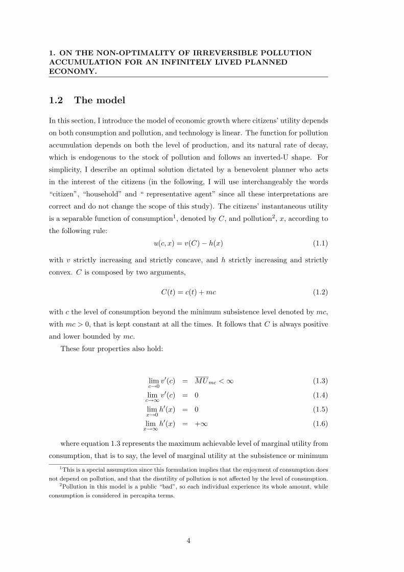
1.2 The model
In this section, I introduce the model of economic growth where citizens’ utility depends
on both consumption and pollution, and technology is linear. The function for pollution
accumulation depends on both the level of production, and its natural rate of decay,
which is endogenous to the stock of pollution and follows an inverted-U shape. For
simplicity, I describe an optimal solution dictated by a benevolent planner who acts
in the interest of the citizens (in the following, I will use interchangeably the words
“citizen”, “household” and “ representative agent” since all these interpretations are
correct and do not change the scope of this study). The citizens’ instantaneous utility
is a separable function of consumption1, denoted by C, and pollution2, x, according to
the following rule:
u(c, x) = v(C)− h(x) (1.1)
with v strictly increasing and strictly concave, and h strictly increasing and strictly
convex. C is composed by two arguments,
C(t) = c(t) +mc (1.2)
with c the level of consumption beyond the minimum subsistence level denoted by mc,
with mc > 0, that is kept constant at all the times. It follows that C is always positive
and lower bounded by mc.
These four properties also hold:
limc→0
v′(c) = MUmc <∞ (1.3)
limc→∞
v′(c) = 0 (1.4)
limx→0
h′(x) = 0 (1.5)
limx→∞
h′(x) = +∞ (1.6)
where equation 1.3 represents the maximum achievable level of marginal utility from
consumption, that is to say, the level of marginal utility at the subsistence or minimum1This is a special assumption since this formulation implies that the enjoyment of consumption does
not depend on pollution, and that the disutility of pollution is not affected by the level of consumption.2Pollution in this model is a public “bad”, so each individual experience its whole amount, while
consumption is considered in percapita terms.
4
1.2 The model
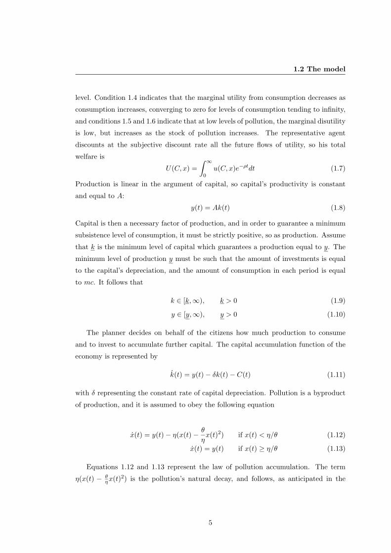
level. Condition 1.4 indicates that the marginal utility from consumption decreases as
consumption increases, converging to zero for levels of consumption tending to infinity,
and conditions 1.5 and 1.6 indicate that at low levels of pollution, the marginal disutility
is low, but increases as the stock of pollution increases. The representative agent
discounts at the subjective discount rate all the future flows of utility, so his total
welfare is
U(C, x) =∫ ∞
0u(C, x)e−ρtdt (1.7)
Production is linear in the argument of capital, so capital’s productivity is constant
and equal to A:
y(t) = Ak(t) (1.8)
Capital is then a necessary factor of production, and in order to guarantee a minimum
subsistence level of consumption, it must be strictly positive, so as production. Assume
that k is the minimum level of capital which guarantees a production equal to y. The
minimum level of production y must be such that the amount of investments is equal
to the capital’s depreciation, and the amount of consumption in each period is equal
to mc. It follows that
k ∈ [k,∞), k > 0 (1.9)
y ∈ [y,∞), y > 0 (1.10)
The planner decides on behalf of the citizens how much production to consume
and to invest to accumulate further capital. The capital accumulation function of the
economy is represented by
k(t) = y(t)− δk(t)− C(t) (1.11)
with δ representing the constant rate of capital depreciation. Pollution is a byproduct
of production, and it is assumed to obey the following equation
x(t) = y(t)− η(x(t)− θ
ηx(t)2) if x(t) < η/θ (1.12)
x(t) = y(t) if x(t) ≥ η/θ (1.13)
Equations 1.12 and 1.13 represent the law of pollution accumulation. The term
η(x(t) − θηx(t)2) is the pollution’s natural decay, and follows, as anticipated in the
5

1. ON THE NON-OPTIMALITY OF IRREVERSIBLE POLLUTIONACCUMULATION FOR AN INFINITELY LIVED PLANNEDECONOMY.
introduction, an inverted-U shape. x = η/θ represents the threshold beyond which
pollution becomes irreversible (so the decay is zero).
In order to write down the conditions for maximization, I will use the same utility
function used by Stokey (15) so the specification of the welfare function becomes:
v(C) =C(t)1−σ − 1
1− σ(1.14)
h(x) =Bx(t)γ
γ(1.15)
with σ > 0, B > 0 and γ > 1. Moreover, I will assume in the following:
HP 2.1. The marginal product of capital net of the depreciation is positive, A−δ > 0.
HP 2.2. The marginal product of capital, net of the depreciation is greater that the
intertemporal rate of preferences, A− δ > ρ
HP 2.3. The sum of the intertemporal rate of preferences and the marginal rate of
decay of pollution is positive, ρ+η(1−2· θηx) > 0. As long as the marginal decay function
is positive, this hypothesis is always satisfied, but when it is negative, this implies that
the rate of impatience is greater than the marginal loss in the self purification capacity
of the environment.
Later, I will compare two possible outcomes of this model: a reversible solution and
an irreversible one. In the first case, I will study the reversible solution, assuming that
the planner will maximise utility in infinite time letting pollution to stay below its
threshold level forever. In the second case, I will study an irreversible solution, and
since the solution admits a point of non-differentiability, I will follow the same approach
used by Thavonen and Withagen and I will split the problem into two subproblems: a
first period problem, where the planner maximises utility from zero to T (finite time)
letting pollution to reach the irreversibility threshold at T , followed by a second period
problem where the planner maximises utility from T to infinity when the natural decay
function for pollution is nil.
6

1.2 The model
1.2.1 Reversible pollution accumulation
Let us assume that the planner wants to maximise the representative citizen’s welfare
having an infinite time horizon plan, and letting pollution not to reach x. In this case,
the problem faced by the planner is:
maxc(t)
W∞ =∫ ∞
0e−ρt
[C(t)1−σ − 1
1− σ− Bx(t)γ
γ
]dt (1.16)
subject to
k(t) = (A− δ)k(t)− C(t) (1.17)
x(t) = Ak(t)− η(x(t) +θ
ηx(t)2) (1.18)
limt→∞
x(t) < x (1.19)
Denote the solution of this first period problem by (c∞, k∞, x∞) and the respective
costate variables by λ∞1 and λ∞2 . Denote also the flow of utility yield by this optimal
plan W∞. The Hamiltonian for this problem is
H(t, k(t), x(t), c(t),Λ; Θ)def= λ0 ·
[C(t)1−σ − 1
1− σ− Bx(t)γ
γ
]+
+λ1(t)[(A− δ)k(t)− c(t)
]+ λ2(t)
[Ak(t)− η(x(t) +
θ
ηx(t)2)
](1.20)
where Λ is the set of shadow prices, Λ = λ0(t), λ1(t), λ2(t) and Θ represents the set of
exogenous parameters of the model, Θ = A,B, σ, ρ, δ, η, θ, γ,mc and, in more detail,
λ1(t) represents the shadow price of capital, and λ2(t) the shadow price of pollution.
The maximum principle asserts that there exists a λ0 and a continuous and piecewise
continuously differentiable functions λ1(t) and λ2(t), such that for all t
(λ0, λ1(t), λ2(t)) 6= (0, 0, 0) (1.21)
H(t, k∗(t), x∗(t), c∗(t),Λ; Θ) ≥ H(t, k∗(t), x∗(t), c(t),Λ; Θ) ∀t (1.22)
The necessary first order conditions are:
∂H
∂c= 0 ⇒ λ1 = C−σ (1.23)
∂H
∂k= ρλ1 − λ1 ⇒ λ1 = λ1(ρ+ δ −A)− λ2A (1.24)
∂H
∂x= ρλ2 − λ2 ⇒ λ2 = λ2 · [ρ+ η(1− 2θ
ηx)] +Bxγ−1 (1.25)
λ0 = 1 or λ0 = 0 (1.26)
7

1. ON THE NON-OPTIMALITY OF IRREVERSIBLE POLLUTIONACCUMULATION FOR AN INFINITELY LIVED PLANNEDECONOMY.
and sufficient conditions for maximisation are the following transversality conditions:
limt→∞
e−ρtλ1(t) · k(t) = 0 (1.27)
limt→∞
e−ρtλ2(t) · x(t) = 0 (1.28)
λ1(t) ≥ 0 (1.29)
λ2(t) ≤ 0 (1.30)
Since the terminal conditions for capital and pollution as time approaches infinity are
left free, it follows that limt→∞ λ1(t) = 0 and limt→∞ λ2(t) = 0 so necessarily, because
of condition 1.26, λ0 = 1.
The following system of four differential equations represents the conditions any
optimal path has to obey:
k = (A− δ)k − λ−1σ
1 (1.31)
x = Ak − ηx+ θx2 (1.32)
λ1 = λ1(ρ− (A− δ))− λ2A (1.33)
λ2 = λ2(η − 2θx+ ρ) +Bxγ−1 (1.34)
with equations 1.33 and 1.34 representing the Euler equations. In equilibrium, all the
variables in the economy grow at a zero rate, so k = x = ψ = λ = 0.
I first start by analyzing the so-called corner solutions, that is to say solutions that
assume consumption equal to the minimum subsistence level. Assuming
HP 2.4. C∗(t) = mc
and also
HP 2.5. mc < η2(A−δ)4θA (This condition is necessary to guarantee the level of pollution
be real)
it follows that there are two simultaneous steady states represented in the table below:
8

1.2 The model
Equilibrium 1 Equilibrium 2k∗ = mc/(A− δ) k∗ = mc/(A− δ)
x∗ =η−
qη2−mc·4θA
A−δ2θ x∗ =
η+qη2−mc·4θA
A−δ2θ
λ∗1 = mc−σ λ∗1 = mc−σ
λ∗2 = − Bx∗γ−11
η−2θx∗1+ρ λ∗2 = − Bx∗γ−11
η−2θx∗1+ρ
Due to the inverse U-shaped function for the pollution decay, this corner solution
admits two stationary points, for each value of mc respecting condition 2.5.
Now, I consider interior solutions. From equation 1.32, it is possible to see that
considering x = 0 and rearranging I get
k =x(η − θx)
A(1.35)
and, combining equations 1.31, 1.33, 1.34 and considering k = ψ = λ = 0 I get
k =1
(A− δ)·(
AB
A− δ − ρ
)− 1σ
· x1−γσ · (η − 2θx+ ρ)
1σ (1.36)
Any intersection between the two equations 1.35 and 1.36 represents an equilibria1.
In general, the existence of an equilibria (or multiplicity of equilibria) depends on the
choice of the parameters of the model. Equation 1.36 is decreasing in all his domain,
whilst equation 1.35 has an inverted-U shape. Graphically, one may have the following
cases:
1This rearrangement of equations 1.31 - 1.34 is only aimed at expressing the two stationary solutions
in the k − x plane and equations 1.35 and 1.36 do not have necessarily an economic interpretation
9

1. ON THE NON-OPTIMALITY OF IRREVERSIBLE POLLUTIONACCUMULATION FOR AN INFINITELY LIVED PLANNEDECONOMY.
Figure 1.1: Graphical representation of different cases, ranging from four to zero steadystates. These cases are not exhaustive.
The first two sets of graphs (case 1 and 2) have been obtained using the following set of parameters: B = 10, 000, 000, A = 0.8,
ρ = 0.04, θ = 0.05, η = 0.03, σ = 3, γ = 3, and δ = 0.1. The second two graphs (case 3 and 4) have instead been obtained
using B = 10, 000, 000, A = 0.8, ρ = 0.02, θ = 0.05, η = 0.03, σ = 3, γ = 3, and δ = 0.1. Irrespective of the set of parameters
chosen, the last two graphs suggest that if the level of capital at the minimum level of consumption is as high as the maximum
level of capital corresponding to the turning point of the decay function for pollution, we can only have one steady state, and if
it is higher, no steady states at all. The last two graphs, instead, do not respect H.2.5 because, in graph 5, mc =η2(A−δ)
4θA and
in graph 6 mc >η2(A−δ)
4θA , with the consequence, respectively, of the existence of only one (or two equal) solutions for pollution,
or zero
10

1.2 The model
The first graph represents a case where two interior solutions exist, and those are
represented by E1 and E2. At the same time, this picture shows that there might exist
two additional corner solutions, represented by the intersection between the horizontal
line (which identifies the minimum level of capital that is necessary to guarantee a
consumption equal to the subsistence level and to cover capital’s depreciation). Those
solutions are, respectively, E3 and E4.
The second picture depicts instead another case where there are still two interior
solutions, but one (represented by E2) cannot be considered a feasible equilibria since
its level of consumption is lower than the subsistence level. This case therefore leads
to only three feasible stable solutions.
Case three represents a different situation where only one interior solution exists,
with associated level of consumption higher than mc. Despite the fact that this solution
requires a different parameter’s set with respect the previous case, the outcome is similar
since it generates three feasible steady solutions.
Case four happens when mc is larger than the equilibrium levels of all the interior
solutions, but the two corner solutions still respect proposition 2.3. Hence, the number
of feasible stable solutions is only two and those are the corner solutions.
Case five occurs when mc is equal to η2(A−δ)4θA . This situation leads to just one stable
solution, irrespective of the number of the existing interior solutions. This is because if
they existed, they would have necessary a level of equilibrium consumption necessarily
lower than the subsistence level. Case six shows, instead, that whatever the number
of interior solutions, if mc > η2(A−δ)4θA , no feasible steady state can exist, because of the
reason above.
It follows that the next propositions hold:
Proposition 2.1. Necessary and sufficient condition to have one interior stable solution
is η < ρ.
Proposition 2.2. Necessary and sufficient condition to have either two or zero interior
stable solutions is ρ > η, sufficient condition to have two interior solutions is ρ <
Ψ · (η/θ)2σ+γ−1 with λ1 = (1/2)σ+γ−1 · (A− δ)σ · ( ABA−δ−ρ)
Proposition 2.3.Necessary and sufficient condition to have two (one) corner solu-
tion(s) is mc < (=)η2(A− δ)/(4Aθ).
11

1. ON THE NON-OPTIMALITY OF IRREVERSIBLE POLLUTIONACCUMULATION FOR AN INFINITELY LIVED PLANNEDECONOMY.
Depending on the choice of the parameters, I can have up to a maximum of four
different equilibria. Consider for example case 1 in figure 1, and assume that k is lower
than the level of capital in equilibrium E2. This implies the existence of four non-trivial
stationary solutions. On the other hand, however, if the level of k is higher than the
level of capital in equilibrium at E2, E2 cannot be considered a valid solution and
therefore the number of equilibria are three.
In what follows, I will confine my analysis to the case where multiplicity of steady
states occurs because, from an economic point of view, I believe it is the most in-
teresting and the most realistic. It is not unusual indeed to see different countries
with characteristics that can be represented by such a configuration of stable solutions.
For instance, it is generally agreed that the cleanest cities in the world are located in
developed and rich countries, like Canada, Finland, Norway etc. The worst polluted
countries are mainly in China and India, that although they are growing at very high
rate, they are not certainly rich countries. On the converse, there are natural paradises
in very poor countries, like still are in Africa. This to highlight the fact that multiplic-
ity of equilibria is the situation that more represents the actual state of the world, and
that is the reason why I decided to focus on it.
In the next section, I will discuss the stability properties of the equilibria, limiting
the analysis to a local level. Such a kind of analysis, is then deepened in section 3 by
studying the global dynamics of the model. Local analysis is indeed of little relevance
when multiplicity of equilibria arises, because it is only able to draw conclusions only on
a close neighbourhood of the equilibria, and it is silent about the dynamics in between
them.
The first interesting information one can extract from the study of the local dynam-
ics of the equilibria is the occurrence of an eventual poverty trap. From the pictures
displayed previously, some equilibria a characterised by low levels of consumption and
capital, and some by higher levels of consumption and capital. If more than one equi-
libria is found to be (saddle) stable, and one provides a lower level of welfare (either
because consumption is lower and/or pollution is higher), we may talk about poverty
trap, that is to say an equilibria which is socially dominated but from which is difficult
to escape.
12

1.2 The model
The second interesting information that will be analysed in the section concerning
the global dynamics, is the behaviour of the system in a generic point of the k − xspace, which represent the initial conditions, respectively, for capital and pollution.
The question I will try to answer is whether the social planner will bring pollution
to its irreversibility region or not, starting, as an example, in a neighbourhood of an
unstable equilibria or far enough from a stable equilibria.
Local dynamics of the equilibria. The study of the local dynamics of the system
around the steady states is usually carried on by linearising the model around them,
using a first order taylor expansion. The first order taylor expansion or Jacobian matrix
of the sistem 1.31 - 1.34 is therefore:˙k˙x˙λ1
˙λ2
=
A− δ 0 1σλ∗− 1+σ
σ1 0
A −η + 2θx∗ 0 0
0 0 ρ− (A− δ) −A0 −2θλ∗2 +B(γ − 1)x∗γ−2 0 η − 2θx∗ + ρ
· k
x
λ1
λ2
The characteristic polynom of the matrix of coefficient can be written as
(µ2 − ρµ)2 + (µ2 − ρµ)z + s (1.37)
with
z = (A− δ)(ρ− (A− δ))− (η − 2θx∗)(ρ+ η − 2θx∗) (1.38)
s = (A− δ)(A− δ − ρ)(η − 2θx∗)(ρ+ η − 2θx∗) +
+1σλ∗− 1+σ
σ1
A2[− 2θλ∗2 +B(γ − 1)x∗γ−2]
(1.39)
Equating the characteristic polynom to zero, and computing the eigenvalues, I get:
µ1,2,3,4 =12ρ±
√(ρ/2)2 − 1
2z ± 1
2
√z2 − 4s (1.40)
and the following lemmas hold:
1. If z < 0, 0 < s ≤ (z/2)2 it is a nec. and suff. condition for all µ to be real, 2
positive and two negative.
2. If s > (z/2)2 and s− (z/2)2− ρ2 · (z/2) > 0 it is a nec. and suff. condition for all
µ to be complex, two with negative real parts and two with positive real parts.
13

1. ON THE NON-OPTIMALITY OF IRREVERSIBLE POLLUTIONACCUMULATION FOR AN INFINITELY LIVED PLANNEDECONOMY.
3. If s < 0 it is a nec. and suff. condition for one eig. to be negative and either 3
eig. to be positive or one positive and two having positive real parts.
4. If s > (z/2)2 and s− (z/2)2− ρ2 · (z/2) = 0 it is a nec. and suff. condition for all
µ to be complex and two having zero real part.
It follows from these lemmas that any equilibrium lying on the increasing locus of
the marginal rate of decay is saddle-stable (z < 0), while the equilibria lying on the
decreasing part of the natural rate of decay of pollution are stable if and only if s > 0.
Since s depends on equilibrium levels of λ1, λ2 and x, analytical conditions determining
the sign of s cannot be found and therefore we have to rely on numerical simulations.
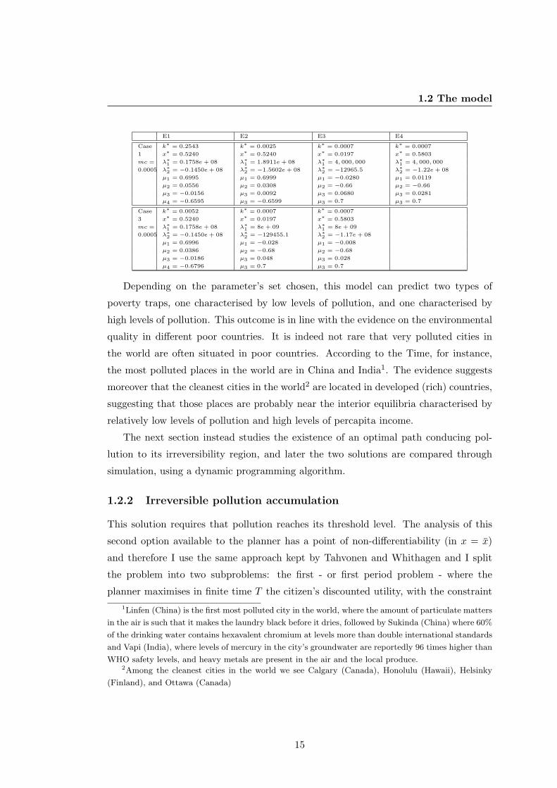
The next table presents two possible outcomes which are depicted in figure 1 above.
The first block is about the results obtained using the parameters of the first two pic-
tures (case 1 and 2) and considering a minimum level of consumption mc very low (in
particular, mc = 0.0005). It follows from those estimation that the model exhibits two
stationary and stable solutions out of four, implying that under the set of parameters
used, only the equilibria on the increasing locus of the decay function of pollution are
stable. However, the second block shows that, changing just one parameter (in partic-
ular, bringing ρ from 0.04 to 0.02, which is the set of parameters used in the third and
fourth pictures above) the corner equilibria lying on the decreasing locus of the function
of the pollution’s decay is stable. This means that lowering the level of impatience of
the representative citizen, it is better to stay in the (socially) dominated equilibria than
deviating. Of course this result hold in a close neighbourhood of the equilibria provided
that capital respects the constraint of being greater than k. This result can already
be an indicator of a non-optimality of irreversible pollution accumulation since if the
population has a “low enough” rate of intertemporal preferences, the higher levels of
utility they can achieve by increasing capital and consumption are not big enough to
compensate the losses due to the growth of pollution.
14
1.2 The model
E1 E2 E3 E4
Case k∗ = 0.2543 k∗ = 0.0025 k∗ = 0.0007 k∗ = 0.0007
1 x∗ = 0.5240 x∗ = 0.5240 x∗ = 0.0197 x∗ = 0.5803
mc = λ∗1 = 0.1758e + 08 λ∗1 = 1.8911e + 08 λ∗1 = 4, 000, 000 λ∗1 = 4, 000, 000
0.0005 λ∗2 = −0.1450e + 08 λ∗2 = −1.5602e + 08 λ∗2 = −12965.5 λ∗2 = −1.22e + 08
µ1 = 0.6995 µ1 = 0.6999 µ1 = −0.0280 µ1 = 0.0119
µ2 = 0.0556 µ2 = 0.0308 µ2 = −0.66 µ2 = −0.66
µ3 = −0.0156 µ3 = 0.0092 µ3 = 0.0680 µ3 = 0.0281
µ4 = −0.6595 µ3 = −0.6599 µ3 = 0.7 µ3 = 0.7
Case k∗ = 0.0052 k∗ = 0.0007 k∗ = 0.0007
3 x∗ = 0.5240 x∗ = 0.0197 x∗ = 0.5803
mc = λ∗1 = 0.1758e + 08 λ∗1 = 8e + 09 λ∗1 = 8e + 09
0.0005 λ∗2 = −0.1450e + 08 λ∗2 = −129455.1 λ∗2 = −1.17e + 08
µ1 = 0.6996 µ1 = −0.028 µ1 = −0.008
µ2 = 0.0386 µ2 = −0.68 µ2 = −0.68
µ3 = −0.0186 µ3 = 0.048 µ3 = 0.028
µ4 = −0.6796 µ3 = 0.7 µ3 = 0.7
Depending on the parameter’s set chosen, this model can predict two types of
poverty traps, one characterised by low levels of pollution, and one characterised by
high levels of pollution. This outcome is in line with the evidence on the environmental
quality in different poor countries. It is indeed not rare that very polluted cities in
the world are often situated in poor countries. According to the Time, for instance,
the most polluted places in the world are in China and India1. The evidence suggests
moreover that the cleanest cities in the world2 are located in developed (rich) countries,
suggesting that those places are probably near the interior equilibria characterised by
relatively low levels of pollution and high levels of percapita income.
The next section instead studies the existence of an optimal path conducing pol-
lution to its irreversibility region, and later the two solutions are compared through
simulation, using a dynamic programming algorithm.
1.2.2 Irreversible pollution accumulation
This solution requires that pollution reaches its threshold level. The analysis of this
second option available to the planner has a point of non-differentiability (in x = x)
and therefore I use the same approach kept by Tahvonen and Whithagen and I split
the problem into two subproblems: the first - or first period problem - where the
planner maximises in finite time T the citizen’s discounted utility, with the constraint1Linfen (China) is the first most polluted city in the world, where the amount of particulate matters
in the air is such that it makes the laundry black before it dries, followed by Sukinda (China) where 60%
of the drinking water contains hexavalent chromium at levels more than double international standards
and Vapi (India), where levels of mercury in the city’s groundwater are reportedly 96 times higher than
WHO safety levels, and heavy metals are present in the air and the local produce.2Among the cleanest cities in the world we see Calgary (Canada), Honolulu (Hawaii), Helsinky
(Finland), and Ottawa (Canada)
15

1. ON THE NON-OPTIMALITY OF IRREVERSIBLE POLLUTIONACCUMULATION FOR AN INFINITELY LIVED PLANNEDECONOMY.
that xT = x, and the second period problem, where the maximisation goes from T to
infinity, with initial conditions xT = x and kT equal to the final value of capital in the
first period. Of course, in the second period problem the natural decay function for
pollution is zero since it has reached the threshold of irreversibility.
The problem can be expressed, then, as follows1:
maxc(t)
W T =∫ T
0e−ρt
[C(t)1−σ − 1
1− σ− Bx(t)γ
γ
]dt (1.41)
subject to
k(t) = (A− δ)k(t)− C(t) (1.42)
x(t) = Ak(t)− η(x(t) +θ
ηx(t)2) (1.43)
k(0) = k0 (1.44)
k(T ) ≥ k (1.45)
x(0) = x0, x0 < x (1.46)
x(T ) = x, T <∞ (1.47)
which represents the so-called “first period problem”2, immediately followed by the
“second period problem” that is
maxc(t)
WT =∫ ∞T
e−ρt[C(t)1−σ − 1
1− σ− Bx(t)γ
γ
]dt (1.48)
subject to the laws of motion of the two state variables and the initial conditions
k(t) = Ak(t)− δk(t)− C(t) (1.49)
x(t) = Ak(t) (1.50)
x(T ) = x (1.51)
k(T ) = kT (1.52)
1It is worthwhile here to make some clarifications: let T the number of periods the planner chooses
to let pollution reach its own threshold of irreversibility. It might be the case that (i) The planner
fixes an arbitrary T and set x(T ) = x or (ii)The planner chooses the optimal T such that x(T ) = x.
Both cases are admissible, however, in the second case further optimality conditions are required and
are explained in the text.2Transversality conditions are not required in the first period problem
16

1.2 The model
and that is also subject to the following sign and transversality conditions, which are
sufficient conditions for maximisation:
λ1(t) ≥ 0 (1.53)
limt→∞
e−ρtλ1(t)k(t) = 0 (1.54)
λ2(t) ≤ 0 (1.55)
limt→∞
e−ρtλ2(t)(x(t)− x) = 0 (1.56)
It is possible to prove (proof provided in the appendix) that an optimal path for
the first period problem exists, because all the state variables are closed subset of R,
and the control C(t) ∈ C ⊆ R.
Let us denote the maximised welfare function for the first and second period, re-
spectively, W T and WT for T < ∞. The maximised utility function for the whole
period is then W = W T + WT . If T is considered fixed, nothing has to be added to the
problem, otherwise, if the planner wish to chose the optimal T , let’s say T ∗, the maxi-
mum principle requires that in addition to the first order conditions and tranversality
conditions, also this condition must be satisfied:
H(k∗(T ∗), x∗(T ∗), c∗(T ∗), λ1(T ∗), λ2(T ∗), T ∗) = 0 (1.57)
The existence of an optimal control with free final time is proved in the appendix A,
provided we modify the assumptions such that T ∗ is free to vary in [T1, T2] and the
theorem is satisfied on the interval [0, T2]. If the planner wishes to maximise the utility
by choosing the optimal terminal time T ∗, it must be the case that
∂W
∂T
∣∣∣∣T ∗
=∂W T
∂T
∣∣∣∣T ∗
+∂WT
∂T
∣∣∣∣T ∗
(1.58)
where
eρT∂W T
∂T=
cT (T )1−σ − 11− σ
− Bxγ
γ+ λT1 (T )[(A− δ)kT (T )− cT (T )] +
+ λT2 (T )[AkT (T )− η(x+θ
ηx2)︸ ︷︷ ︸
=0
] (1.59)
−eρT ∂WT
∂T=
cT (T )1−σ − 11− σ
− Bxγ
γ+ λ1T (T )[(A− δ)kT (T )− cT (T )] +
+ λ2T (T )[AkT (T )] (1.60)
17

1. ON THE NON-OPTIMALITY OF IRREVERSIBLE POLLUTIONACCUMULATION FOR AN INFINITELY LIVED PLANNEDECONOMY.
Equation 1.58 is verified when CT (T ) = CT (T ) and kT (T ) = kT (T ), i.e. they are
continuous functions at T ∗. If instead it is not optimal to reach x in finite time, it must
be the case that
limT→∞
sup∂W
∂T= lim
T→∞sup
∂W T
∂T+ limT→∞
sup∂WT
∂T≥ 0 (1.61)
so it is necessary that W does not decrease when T increases without limit.
For what concerns the first period problem, define the current value Hamiltonian
associated to the problem 1.41 - 1.47 as
H(t, k(t), x(t), c(t),Λ; Θ)def= ·[C(t)1−σ − 1
1− σ− Bx(t)γ
γ
]+
+λ1(t)[(A− δ)k(t)− c(t)
]+ λ2(t)
[Ak(t)− η(x(t) +
θ
ηx(t)2)
](1.62)
where Λ is the set of shadow prices and Θ represents the set of exogenous parameters
of the model where, as before, Θ = A,B, σ, ρ, δ, η, θ, γ,mc.The necessary first order conditions are:
∂H
∂c= 0 ⇒ λ1 = C−σ (1.63)
∂H
∂k= ρλ1 − λ1 ⇒ λ1 = λ1(ρ+ δ −A)− λ2A (1.64)
∂H
∂x= ρλ2 − λ2 ⇒ λ2 = λ2 · [ρ+ η(1− 2θ
ηx)] +Bxγ−1 (1.65)
(1.66)
so the following system of four differential equations represents the conditions any
optimal path has to obey:
k = (A− δ)k − λ−1σ
1 (1.67)
x = Ak − ηx+ θx2 (1.68)
λ1 = λ1(ρ− (A− δ))− λ2A (1.69)
λ2 = λ2(η − 2θx+ ρ) +Bxγ−1 (1.70)
k(0) = k0 (1.71)
k(T ) ≥ k (1.72)
x(0) = x0, x0 < x (1.73)
x(T ) = x, T <∞ (1.74)
18

1.2 The model
with equations 1.69 and 1.70 representing the Euler equations.
For the second period problem, define the current value Hamiltonian associated to
the problem 1.48 - 1.52 as:
H(t, k(t), x(t), c(t),Λ; Θ)def= λ0
[C(t)1−σ − 1
1− σ− Bx(t)γ
γ
]+
+λ1(t)[Ak(t)− δk(t)− C(t)
]+ λ2(t) ·Ak(t) (1.75)
where Λ is the set of shadow prices and, as before Λ = λ0(t), λ1(t), λ2(t) with
λ1 and λ2 representing, respectively, the shadow prices of capital and pollution and
Θ represents the set of exogenous parameters of the model where, as before, Θ =
A,B, σ, ρ, δ, η, θ, γ,mc.The maximum principle asserts that there exists a λ0 and a continuous and piecewise
continuously differentiable functions λ1(t) and λ2(t), such that for all t
(λ0, λ1(t), λ2(t)) 6= (0, 0, 0) (1.76)
H(t, k∗(t), x∗(t), c∗(t),Λ; Θ) ≥ H(t, k∗(t), x∗(t), c(t),Λ; Θ) ∀t (1.77)
Moreover1,
∂H
∂c= 0 ⇒ λ1 = C−σ (1.78)
∂H
∂k= ρλ1 − λ1 ⇒ λ1 = λ1(ρ+ δ −A)− λ2A (1.79)
∂H
∂x= ρλ2 − λ2 ⇒ λ2 = λ2 · ρ+Bxγ−1 (1.80)
λ0 = 1 or λ0 = 0 (1.81)
Since the terminal conditions for capital and pollution as time approaches infinity
are left free, it follows that limt→∞ λ1(t) = 0 and limt→∞ λ2(t) = 0 so λ0 = 1. Finally,
1.51 and 1.52 have to be satisfied.
Rearranging equation 1.78 we get an expression for consumption in terms of the
shadow price of capital:
C = λ− 1σ
1 (1.82)1For notational simplicity, in the following I will use interchangeably the generic variable z instead
of z(t) whenever this does not constitute ambiguity.
19

1. ON THE NON-OPTIMALITY OF IRREVERSIBLE POLLUTIONACCUMULATION FOR AN INFINITELY LIVED PLANNEDECONOMY.
so the economic system can be represented by the following four differential equations
k = (A− δ)k − λ−1σ
1 (1.83)
x = Ak (1.84)
λ1 = λ1(ρ+ δ −A)− λ2A (1.85)
λ2 = λ2ρ+Bxγ−1 (1.86)
From equation 1.84 is straightforward to see that in order to keep pollution stable
through time (x = 0) it is necessary to keep capital nil. This means that no production
nor consumption can occur in steady state, and since for hypothesis the model guar-
antees a minimum level of consumption, implying also a strictly positive capital and
production, no stationary solution can be found in this second period problem. In the
long run, the optimal path will converge to a consumption level equal to the subsistence
level mc, with a capital level constant and equal to k. This level of capital is such that
it produces a level of income which sustains a minimum level of consumption and an
investment level which is equal to the depreciation of capital.
The existence of a balanced growth path for capital, pollution and consumption can
be reasonably excluded because this would imply a constant and equal rate of growth
for all the variables involved, consumption, pollution and capital. Since the marginal
utility from consumption is an increasing and concave function of consumption, and
the marginal disutility from pollution is an increasing and convex function of pollution
(so it grows at a rate that is greater than the rate of growth of the marginal utility from
consumption), there will be a point on time t′ ∈ [T,∞) where an additional unit of
pollution will produce a disutility higher than the utility produced by an additional unit
of consumption. At this point in time, the optimal path will predict a consumption level
equal to mc, production equal to y and a minimum level of capital k that is necessary to
guarantee a level of investments that covers the depreciation, and a subsistence level of
consumption. Pollution, from t′ onward, will have an instantaneous variation x = Ak,
while the variation of capital and consumption will be nil.
1.2.3 Paths comparison
The model does not allow to say which of the paths gives higher utility, so direct
comparison is necessary. In particular, we are interested to see whether an irreversible
20

1.3 Global analysis
solution may provide an higher level of discounted utility than an irreversible one. But
this requires first of all the computation of W∞ and W = W T + WT . The analysis
presented in paragraph 2.2.1 is only partial, because it is just able to say something
about the stability of the two steady states and their associated level of welfare W∞
if the system is in equilibrium and there are no shocks able to carry on the system far
away from them, but is is completely unable to say anything about the behaviour of the
system in between of the two fixed points, or in any point of the x−k plane. In order to
say something about the behaviour of this economy far away from the equilibria, global
analysis is needed. In the next section, I will use an algorithm of dynamic programming
to carry on this analysis.
As it was previously anticipated, the problem presented here has the peculiarity of
having, for each initial condition and in finite time horizon, two simultaneous optimal
paths which respect the first order conditions. In accordance to the possibilities avail-
able to the planner, it may be optimal either to increase utility by reducing pollution
or, viceversa, by increasing consumption. The first choice takes the system in a path
which is converging to the saddle stable equilibria introduced in section 2.2.1 (so in
this case a reversible solution is optimal), and the other choice takes the system toward
the irreversibility threshold for pollution. Whether it is optimal one or the other, is a
question I will try to answer below.
1.3 Global analysis
In this section, I am interested to see whether - in case of multiple equilibria - the system
can, starting from a neighbourhood of the unstable equilibria, recover and converge to
the socially optimum steady state. Due to the lack of closed form solution of this
dynamic model, I need to use computational methods. I use the convenient approach
of dynamic programming, which provides the value function and the control variable in
feedback form. This allows to find the global dynamics of the state space in the region
restricted by arbitrary values of capital and pollution, using a fixed grid size technique.
21

1. ON THE NON-OPTIMALITY OF IRREVERSIBLE POLLUTIONACCUMULATION FOR AN INFINITELY LIVED PLANNEDECONOMY.
1.3.1 Discretisation
The first step to do that is to discretize the model identified by equations 1.16 - 1.18
maxct∈Ct
Ut =∞∑t=0
βt[c1−σt − 11− σ
−Bxγt
γ
](1.87)
subject to
xt+1 = Akt − xt(η − θxt − 1) (1.88)
kt+1 = (A− δ + 1)kt − ct (1.89)
β = (1− ρ) (1.90)
k0 = k (1.91)
x0 = x (1.92)
Here Ct denotes the set of discrete control sequences C = (C1, C2, ...) for Ci ∈ C
The optimal value function V is the unique solution of the discrete Hamilton-Jacobi-
Bellman’s equation
V (k, x) = maxc∈C
ut(kt, xt, Ct) + βV (kt+1, xt+1)
(1.93)
with
ut(kt, xt, Ct) =[c1−σt − 11− σ
−Bxγt
γ
](1.94)
If I define the dynamic programming operator T by
T (V )(k, x) = maxC∈C
ut(kt, xt, Ct) + βV (kt+1, xt+1)
(1.95)
then V can be characterised as the unique solution of the fixed point equation
V (k, x) = T (V )(k, x) for all x, k ∈ Rn (1.96)
1.3.2 Results
The study of dynamic decision models with multiple equilibria is intricate. Multi-
ple equilibria can arise in models with non-concave pay-off functions, externalities
and increasing returns. Recently multiple equilibria have been found also in concave
economies (for a survey on models with multiple equilibria, see Deissenberg et al (6)).
In terms of dynamics, multiple equilibria are difficult to analyse, since the domain of
22

1.3 Global analysis
attraction might not coincide with the stable and unstable equilibria, and multiple
optimal paths may exist as well. In the context of my model, multiple (non-trivial)
equilibria arise from some parameter constellations. In the following, I will consider
only a set of parameters which gives multiple steady states, because I believe this case
is the most interesting from a policy point of view. Consider the following parameter
set:
B = 10, 000, 000
A = 0.8
ρ = 0.04
θ = 0.05
η = 0.03
σ = 3
γ = 3
δ = 0.1
β = 1− ρ = 0.96
Those parameters yield the following numerical solution for the two (non-trivial) steady
states:
Variable Equilibrium 1 Equilibrium 2k∗ 0.5494e-2 0.2489e-2x∗ 0.2543 0.5240λ∗1 0.1758e+08 1.8911e+08λ∗2 -0.1450e+08 -1.5602e+08
The eigenvalues of the first equilibria areµ1= 0.6995, µ2= 0.0556, µ3 =-0.0156 and µ4=-
0.6595 and for the second are µ1 = 0.6999, µ2= 0.0308, µ3 = 0.0092 and µ4= -0.6599.
This information allows us to say only that the first equilibria is saddle stable (however,
this conclusion holds only locally and what happens between the two steady states is
a black box), and that second is unstable. Nothing can be said about the direction of
the instability of this latter equilibria. In other words, from the local analysis nothing
can be inferred about whether - starting from initial conditions close to the unstable
equilibria - the system will converge to the stable (and pareto dominant) equilibria or
not. To this purpose, I studied the global dynamics of this system using a dynamic
23
1. ON THE NON-OPTIMALITY OF IRREVERSIBLE POLLUTIONACCUMULATION FOR AN INFINITELY LIVED PLANNEDECONOMY.
programming algorithm. Dynamic programming allows to draw the phase diagram of
the system in terms of the states variables and it is a convenient tool to study the global
dynamics in case of multiplicity of equilibria. The algorithm is described in detail in
appendix, and results are depicted in figure 2.
The first thing is to check first of all if the system will converge to the socially
dominant equilibria or not, starting in proximity of the unstable one. Numerical simu-
lations show that, for example, assuming a fixed plan horizon of 50 periods, there exist
two optimality candidates: one path that brings pollution toward the irreversibility
region and the other one that converges to the saddle stable (and socially dominant)
equilibria. Basically, an efficiently managed economy may choose to achieve the ob-
jective of maximising the utility function by means of two instruments: (i) increasing
consumption or (ii) reducing pollution. The first policy implies that the consumption
profile of the first periods is left low, capital is allow to increase at a very fast rate,
and so also consumption in the subsequent periods. The second policy, viceversa, is
described by an high level of consumption in the first period (aimed at reducing the
level of capital, responsible for the production of pollution), and a low profile (although
increasing) of consumption in subsequent periods. The choice between these two paths
cannot be made a priori and the computation of the utility’s present value is needed.
Figure 2 and 3 show the phase diagrams in terms of the state variables and the
behaviour of the control variable for the two different paths. Numerical simulations
show that the utility’s present value for the first path (the path diverging towards the
irreversibility threshold of pollution, represented in figure 2) is equal to -1.1427e+07,
against a present value of -1.4796e+07 for the second path in figure 3, the path con-
verging to the saddle stable equilibria. It is therefore worth increasing capital and
consumption up or close to the irreversibility threshold of pollution, if the time horizon
is sufficiently low.
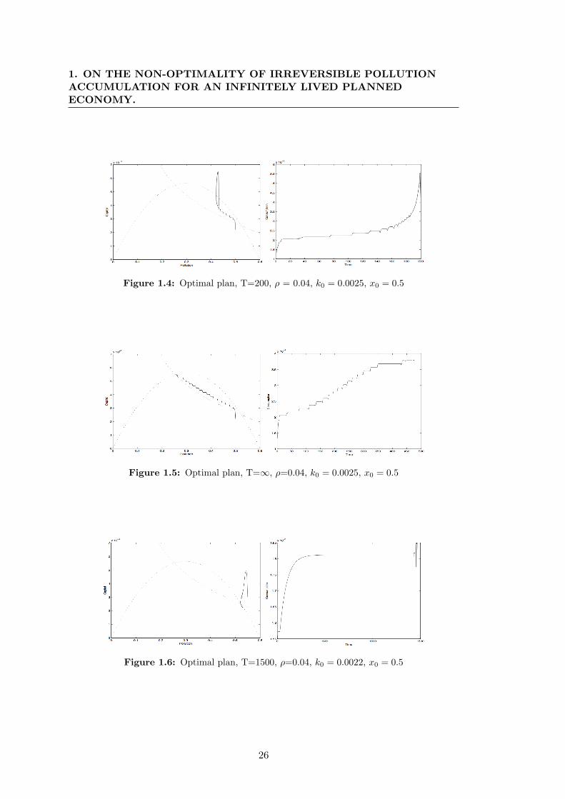
Things seem different, however, when the plan horizon is longer. As T grows, hypo-
thetically to infinity, numerical simulations suggest that the optimal path is no longer
to bring pollution close or up to the irreversibility region, as it is clearly highlighted in
the figures below. Those pictures indeed show a tendency of the system to converge to
the stable and socially optimal interior equilibria1. This may be explained by the fact
1The minimum consumption level is assumed to be set at very low levels such that the solution
never hits it
24

1.3 Global analysis
Figure 1.2: Divergent path, T=50, k0 = 0.0025, x0 = 0.5
Figure 1.3: Convergent path, T=50, k0 = 0.0025, x0 = 0.5
that the utility of having high levels of consumption for limited amounts of periods fol-
lowed by minimum levels of consumption and increasing levels of pollution for infinite
periods is definitely worse than having moderately high levels of consumption and low
levels of pollution forever, especially if the intertemporal rate of preferences is not too
high.
As it is possible to see in figure 4, for T=200, the tendency is to keep capital at
a level which allows both strictly positive consumption and a reduction of pollution,
except for dramatically increase capital, consumption and pollution during the last
periods (but this is due to the fact that we are dealing with a routine that in order to
be ran has to set a finite time horizon).
So, two identical countries may choose different environmental policies only if they
differ in the choice of their planning horizons. Governments who have short term
objectives will choose paths which imply a growing stock of pollution through time,
whilst governments with longer horizons will choose paths which imply a decrease of
pollution and a slower increase in consumption. This convergence to the interior and
stable equilibria is found irrespective of the set of initial conditions.
25
1. ON THE NON-OPTIMALITY OF IRREVERSIBLE POLLUTIONACCUMULATION FOR AN INFINITELY LIVED PLANNEDECONOMY.
Figure 1.4: Optimal plan, T=200, ρ = 0.04, k0 = 0.0025, x0 = 0.5
Figure 1.5: Optimal plan, T=∞, ρ=0.04, k0 = 0.0025, x0 = 0.5
Figure 1.6: Optimal plan, T=1500, ρ=0.04, k0 = 0.0022, x0 = 0.5
26

1.3 Global analysis
Figure 7 displays a path leading pollution to reach its irreversibility threshold. As
predicted in the previous section, after pollution has become irreversible, it is optimal
for the planner to let capital and consumption to reach their “survival” levels set by
k and mc, respectively. The picture shows also that pollution grows steadily through
time.
Figure 1.7: Optimal plan, T=∞, ρ = 0.04, k0 = 0.0025, x0 = 0.5, mc = 0.001
In order to compare the two different environmental policies, it is necessary to
compute the present value of all the flows of utility provided in each period by the two
paths. The optimal path depicted in figure 5 provides a present value of utility equal
to -5.93e+07, whilst the path depicted in figure 7 provides -2.09e+08, with a negative
difference of -1.50e+08.
Contrary to Tahvonen and Withagen’s result, according to which optimality or not
of irreversible pollution accumulation depends on the initial condition for pollution (be-
ing optimal when the initial condition for pollution is higher than the level determined
by the unstable equilibria), my numerical simulations show a different story. Figure 6
provides a clear example. Initial condition for pollution is 0.53, which is higher than
0.524 characterising the second equilibria. The time span necessary to get into what
they call “domain of attraction of the saddle stable equilibria” is however very high,
and increases as the initial pollution level increases. Consumption also grows steadily
but slowly in proximity of the equilibria: unfortunately the accuracy of the picture is
not enough to make it evident. What makes the difference between their model and my
model is not the set of initial condition (which is also a poor explanation of the reasons
why a country should prefer irreversibility), but the fact that the marginal utility of
consumption when consumption is zero, is nil. This is an implication of the fact that
27

1. ON THE NON-OPTIMALITY OF IRREVERSIBLE POLLUTIONACCUMULATION FOR AN INFINITELY LIVED PLANNEDECONOMY.
they deal with a local pollution problem and not with a global one. Being zero the
marginal utility from consumption when there is no consumption at all implies that the
population can move elsewhere to satisfy their needs. In my model it is not possible,
and there survival (and consumption, although at minimum levels) is always preferred
to an additional unit of pollution.
The simulations therefore are clear in highlighting the fact that irreversibility is
never optimal, if the planning horizon is infinite, and no matters the initial level of
pollution. Different environmental policies can therefore be explained only by different
planning horizon of the governments, all other parameters constant.
1.3.3 The effect of ρ on the global dynamics of the system
The representative household’s level of impatience, represented by ρ, may play a crucial
role in determining the environmental policy chosen by the planner. The more impatient
the people are, the more probable is a policy which implies a growing stock of pollution
through time. The effects are someway similar to a shortening of the time horizon, and
this is confirmed by the simulations. Figure 6 represents the global dynamics of the
system assuming a time horizon of 200 periods, and an intertemporal rate of preferences
equal to 0.009. The only parameter that distinguishes figure 6 from figure 4 is the level
of ρ, but as it is possible to see the dynamics is dramatically different. Convergency to
Figure 1.8: Optimal plan, T=200, ρ = 0.09, k0 = 0.0025, x0 = 0.5
the saddle stable equilibria is harder to find, since the high discount rate and the finite
horizon make worth for the planner choosing a path which implies an high growth rate
of consumption for the first periods, which are valued more than future ones, especially
because pollution - compared to consumption, grows at much slower rate.
28

1.4 Conclusion
1.4 Conclusion
This paper contributes in the debate about the necessity of a unified global environmen-
tal policy kept by all the nations. With a theoretical model of economic growth with
pollution accumulation and an endogenous function for the natural decay of pollution,
I show with numerical simulation that in an efficiently planned economy, with infinite
time horizon plan, irreversible pollution accumulation cannot be an optimal policy.
Optimality of such a policy can occur only if the plan of government is short-minded.
Since utility depends on both consumption and the level of pollution, in principle the
planner can choose to achieve the maximum level of welfare by, alternatively, increasing
consumption or reducing pollution. The second strategy pays in the long run, while
the first in short run.
It would be important to keep in mind that although each nation decides on its
own its environmental policy and it is free to join international agreement, we live in
the same planet and if all the countries would be one with the priority to safeguard
life, they would not engage in such production of pollution, in each form. So, despite
incentives are not enough to give up opportunities to grow in the short run, it would
be useful to ask whether such individual policy can be consistent with individual long
terms goal. Each country may decide to pollute a lake if there are others from which
he can extract utility, but what happens when all the lakes are polluted?
Unfortunately, populist policies and the fact that politicians stay in power for few
years and needs to be reelected can - someway - affect the environmental policies un-
dertaken by the countries. Special interests overcome in importance other issues which
are in general considered of marginal relevance, like the environment, because a policy
undertaken by a single country can only marginally affect it, especially when it deals
with global problems.
So, a deep study of the incentives taking a country to engage in global emission’s
reduction is needed and it can be part of future research.
29
1. ON THE NON-OPTIMALITY OF IRREVERSIBLE POLLUTIONACCUMULATION FOR AN INFINITELY LIVED PLANNEDECONOMY.
1.5 Appendix
A. Proof of the existence of an optimal path for the first period problem
- T fixed
To prove the existence of an optimal path for the first period problem when the final
time T is fixed and the pollution at T is equal to its threshold, I use the Filippov -
Cesari theorem of existence of an optimal control (Seierstad and Sydsæter (13), p. 132)
which requires the convexity of the set
N(k, x,C, t) =c1−σ − 1
1− σ− Bxγ
γ+ ω, (A− δ)k − c, Ak − η(x+
θ
ηx2)
(1.97)
where C ⊆ R represents the set of all admissible controls, and ω ≤ 0. The theorem
states: Consider the standard optimal control problem 1.41 - 1.47. Assume that:
• There exists an admissible triple (k(t), x(t), c(t)).
• N(k, x,C, t) is convex for each (k, x, t).
• C is closed and bounded.
• There exists two numbers k and x such that ‖k(t)‖ ≤ k and ‖x(t)‖ ≤ x for all
t ∈ [0, T ] and all admissible pairs (k(t), x(t), c(t)).
Then, there exists an optimal pair (k∗(t), x∗(t), c∗(t)) (with c∗(t) measurable). In order
to prove the convexity of the set in 1.97, let us keep (k(t), x(t), t) fixed, so k(t) = K
and x(t) = X. Let y1, y2, y3 three arbitrary points in N(K,X,C, t), i.e.
y1 =(c1−σ
1 − 11− σ
− BXγ
γ
)e−ρt + ω1, (A− δ)K − c1, AK − η(X − θ
ηX2)
y2 =
(c1−σ2 − 11− σ
− BXγ
γ
)e−ρt + ω2, (A− δ)K − c2, AK − η(X − θ
ηX2)
y3 =
(c1−σ3 − 11− σ
− BXγ
γ
)e−ρt + ω3, (A− δ)K − c3, AK − η(X − θ
ηX2)
for some ω1, ω2, ω3 ≤ 0 and c1, c2, c3 ∈ C. Let λ1 and λ2 two positive constants such
that λ1 +λ2 ≤ 1. I need to prove that y4 = λ1y1 +λ2y2 +(1−λ1−λ2)y3 ∈ N(K,X,C, t).
Put λ1y1 + λ2y2 + (1− λ1 − λ2)y3 = (z1, z2, z3). The first component z1 is:
30

1.5 Appendix
z1 = λ1
(c1−σ1 − 11− σ
− BXγ
γ
)e−ρt + λ1ω1 +
+ λ2
(c1−σ2 − 11− σ
− BXγ
γ
)e−ρt + λ2ω2 +
+ (1− λ1 − λ2)(c1−σ
3 − 11− σ
− BXγ
γ
)e−ρt + (1− λ1 − λ2)ω3 (1.98)
=λ1c1−σ
1 − 11− σ
+ λ2c1−σ
2 − 11− σ
+ (1− λ1 − λ2)c1−σ
3 − 11− σ
e−ρt +
− BXγ
γe−ρt + λ1ω1 + λ2ω2 + (1− λ1 − λ2)ω3 (1.99)
Since it is known that W T is concave in c, so W T ” ≤ 0, we have
λ1c1−σ
1 − 11− σ
+ λ2c1−σ
2 − 11− σ
+ (1− λ1 − λ2)c1−σ
3 − 11− σ
≤ [λ1c1 + λ2c2 + (1− λ1 − λ2)c3]1−σ − 11− σ
=c1−σ
4 − 11− σ
with c4 = λ1c1 + λ2c2 + (1− λ1 − λ2)c3. Then, c4 ∈ C. Using this result, from the last
inequality we see that
z1 ≤(c1−σ
4 − 11− σ
− BXγ
γ
)e−ρt + λ1ω1 + λ2ω2 + (1− λ1 − λ2)ω3 (1.100)
Define ω4 = z1 −(c1−σ4 −1
1−σ − BXγ
γ
)e−ρt. Then, from 3.11,
ω4 ≤ λ1ω1 + λ2ω2 + (1− λ1 − λ2)ω3 ≤ 0 since ω1, ω2, ω3 ≤ 0
The second and third components, z2 and z3 are found similarly to the first:
z2 = λ1[(A− δ)K − c1] + λ2[(A− δ)K − c2] + (1− λ1 − λ2)[(A− δ)K − c3]
= (A− δ)K − (λ1c1 + λ2c2 + (1− λ1 − λ2)c3)
= (A− δ)K − c4
z3 = λ1[AK − η(X − θ
ηX2)] + λ2[AK − η(X − θ
ηX2)] +
+(1− λ1 − λ2)[AK − η(X − θ
ηX2)]
= AK − η(X − θ
ηX2)
31

1. ON THE NON-OPTIMALITY OF IRREVERSIBLE POLLUTIONACCUMULATION FOR AN INFINITELY LIVED PLANNEDECONOMY.
Piecing all this together, we see that we have found a c4 ∈ C and a ω4 ≤ 0 such that
λ1y1+λ2y2+(1−λ1−λ2)y3 = ( c1−σ4 −11−σ −
BXγ
γ )e−ρt+ω4, (A−δ)K−c4, AK−η(X− θηX
2).Hence, λ1y1 + λ2y2 + (1− λ1 − λ2)y3 ∈ N(K,X,C, t) and thus N(K,X,C, t) is convex.
B. The dynamic programming algorithm
The algorithm approximates the solution on a grid Γ covering a compact subset Ω of
the state space. I pick a reasonable set Ω and consider only trajectories which remain
in Ω in all future times. I assume that for any point (k, x) ∈ Ω there exists at least one
control value c such that (kt+1, xt+1) ∈ Ω holds. Denoting the nodes of the grid Γ by
(ki, xj), i = 1, ..., n and j = 1, ...,m, the approximation V Γ satisfy
V Γ(ki, xj) = T (V Γ)(ki, xj) (1.101)
for all nodes (ki, xj) of the grid, where the value of V Γ for points (k, x) which are
not grid points (these are needed for the evaluation of T ) is determined by bilinear
interpolation. Basically, the standard computational algorithm that is used here can
be summarised as follows (cite larson):
1. The first step is to set up a grid for the state variables. Each level of capital k and
each level of pollution x are quantised, respectively, to Nk and Nx equidistant
levels, from 0 to, respectively, k and x. In total, then, the grid points for the
state variables are Nk ·Nx. The control variable c is quantised to Nc equidistant
levels, from 0 to c.
2. For each point in the grid (k(i), x(j)), i = 1, ..., Nk and j = 1, ..., Nx, each control
c(h), h = 1, ..., Nc is applied, and the next state is computed according to the
formulas given by equations 1.88 and 1.89. Let us call the next-state value of
k and x, respectively, k1 and x1. Notice that k1 and x1 are tri-dimensional
matrices whose generic element is represented by k1(i, j, h) and x1(i, j, h) and
whose dimensions are Nk ·Nx ·Nc. Furthermore, the elements of k1 and x1 are,
in general, not grid points. I then check whether each element of k1 ∈ [0, k] and
x1 ∈ [0, x]. If they do not belong to those intervals, their values are replaced with
“missing”.
3. Define the number of periods T , and set up an index l = 1. Evaluate k0 and x0.
32
1.5 Appendix
4. The procedure is backward. At the final time T , citizens consume what is left in
terms of capital, so cT = kT irrespective to the value of x. So, for each point in
the grid (k(i), x(j)), i = 1, ..., Nk and j = 1, ..., Nx I compute the value function
at time T which is nothing but
V Γ(k(i), x(j), T ) =k(i)(1−σ) − 1
1− σ−Bx(j)γ
γi = 1, ..., Nk, j = 1, ..., Nx (1.102)
I then store in memory V Γ(k(i), x(j), T ) and c(i, j, T ) = k(i) constant across the
j and the T -dimensions.
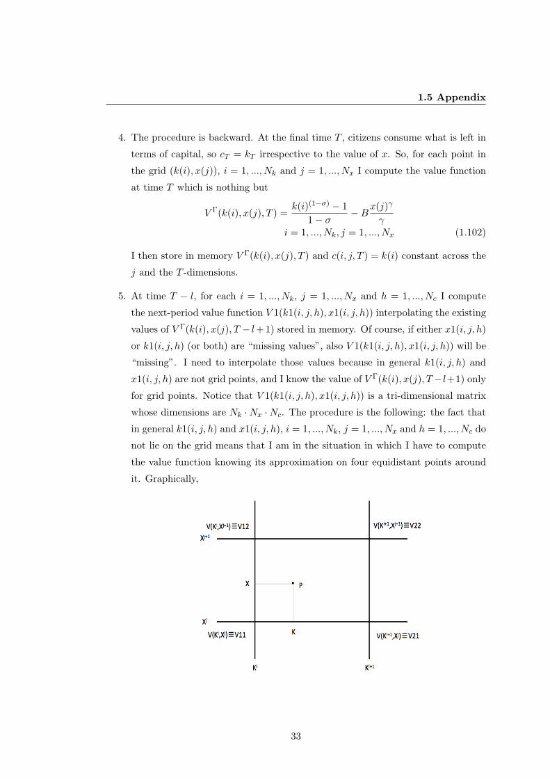
5. At time T − l, for each i = 1, ..., Nk, j = 1, ..., Nx and h = 1, ..., Nc I compute
the next-period value function V 1(k1(i, j, h), x1(i, j, h)) interpolating the existing
values of V Γ(k(i), x(j), T − l+ 1) stored in memory. Of course, if either x1(i, j, h)
or k1(i, j, h) (or both) are “missing values”, also V 1(k1(i, j, h), x1(i, j, h)) will be
“missing”. I need to interpolate those values because in general k1(i, j, h) and
x1(i, j, h) are not grid points, and I know the value of V Γ(k(i), x(j), T−l+1) only
for grid points. Notice that V 1(k1(i, j, h), x1(i, j, h)) is a tri-dimensional matrix
whose dimensions are Nk ·Nx ·Nc. The procedure is the following: the fact that
in general k1(i, j, h) and x1(i, j, h), i = 1, ..., Nk, j = 1, ..., Nx and h = 1, ..., Nc do
not lie on the grid means that I am in the situation in which I have to compute
the value function knowing its approximation on four equidistant points around
it. Graphically,
33

1. ON THE NON-OPTIMALITY OF IRREVERSIBLE POLLUTIONACCUMULATION FOR AN INFINITELY LIVED PLANNEDECONOMY.
I want to approximate a function on the point P = (k, x) that represents my next
period values of the state variable once the control is applied, knowing the value
function in the points V 11, V 12, V 21 and V 22. The function in P is computed
according to the following formula:
V (P ) =V 11
(ki+1 − ki)(xj+1 − xj)· (ki+1 − k)(xj+1 − x)
V 21(ki+1 − ki)(xj+1 − xj)
· (k − ki)(xj+1 − x)
V 12(ki+1 − ki)(xj+1 − xj)
· (ki+1 − k)(x− xj)
V 22(ki+1 − ki)(xj+1 − xj)
· (k − ki)(x− xi) (1.103)
6. For each i = 1, ..., Nk, j = 1, ..., Nx and h = 1, ..., Nc I compute
V ′(k(i), x(j), c(h), T − l) =c(h)1−σ − 1
1− σ−Bx(j)γ
γ+
βV 1(k1(i, j, h), x1(i, j, h)) (1.104)
After that, for each i = 1, ..., Nk, j = 1, ..., Nx I chose the maximum variable
over the h-dimension (control), by direct comparison. Those values are stored
c(i, j, T − l) and V Γ(k(i), x(j), T − l)
7. The value of l takes l + 1.
8. I check whether l is equal to T . If it is not, I go back to point 5. If l = T , then
9. Define three vectors k∗(t), x∗(t) and c∗(t), t = 1, ..., T which represent the op-
timal trajectories of capital, pollution and consumption starting from the initial
conditions x0 and k0. Set k∗(1) = k0 and x∗(1) = x0.
10. Set time t = 1.
11. Find the ith and jth elements in the vectors of quantized k and x, which are closer
to the values k∗(t) and x∗(t). If (k(i), x(j)) = (k∗(t), x∗(t)) then the state is a
grid point, and c∗(t) is read directly as c(i, j, t). If (k(i), x(j)) 6= (k∗(t), x∗(t)),
c∗(t) is computer through bilinear interpolation using values of c(i, j, t) at the
closest grid points for k and x.
34

1.5 Appendix
12. Check whether t = T + 1. If this equality is satisfied, go to point 15. Else, go to
the next point.
13. Compute k∗t+1 and x∗t+1 according to the following equations:
k∗(t+ 1) = (A+ δ − 1)k∗(t)− c∗(t) (1.105)
x∗(t+ 1) = Ak∗(t)− x∗(t)(η − θx∗(t)− 1) (1.106)
14. Time t takes value t+ 1. Go to point 11.
15. The value function is computed as follows: set time t = T and an index l = 1. At
final time T , the value function is computed according to the following formula:
V ∗(T ) =c∗(T )1−σ − 1
1− σ−Bx
∗(T )γγ
(1.107)
16. Check wheter t = 0. If so, end the program, otherwise go to the next point.
17. Time t takes values T − l.
18. The value function at time t is now
V ∗(t) =c∗(t)1−σ − 1
1− σ−Bx
∗(t)γ
γ+ βV ∗(t+ 1) (1.108)
19. The index l takes value l + 1. Go to point 16.
This computational procedure is very appealing for a number of reasons. First, because
thorny questions about existence and uniqueness are avoided; as long as there is at
least one feasible control sequence, then the direct-search procedure guarantees that
the absolute maximum utility is achieved. Furthermore, extremely general types of
systems equations and constraints can be handled. Constraints actually reduce the
computational burden by decreasing the admissible sets of states and controls. Finally,
the optimal control is obtained as a true feedback solution in which the optimal control
for any admissible state and stage is determined. However, to the best of my knowledge
there is not any algorithm able to identify whether multiple solutions exist, and this
one makes no exception. Identify them may be difficult, because it requires repeated
simulation of the same routine, and a bit of luck. If indeed multiple solutions exist,
since in general they do not provide the same values of discounted flows of utility, the
35

1. ON THE NON-OPTIMALITY OF IRREVERSIBLE POLLUTIONACCUMULATION FOR AN INFINITELY LIVED PLANNEDECONOMY.
path which provides the highest value is generally chosen by the routine. So, most
of the time, one does not even realise that multiple paths satisfying the first order
conditions exist. They can only be found choosing appropriate grids, and this is a
very difficult task because it requires first of all the knowledge about the existence of
multiple solutions, and a good guess about the direction of the two paths. Finally, luck
is always welcome.
Codes
In this section, I report the matlab codes that I used to draw the pictures and to
compute the present value of the flow of utilities, in order to compare the two paths.
The first program is the following, named
PROGRAM fp main:
code:
PROGRAM fp parameters:
code:
PROGRAM fp step1:
36

1.5 Appendix
code:
PROGRAM fp nextstates:
code:
PROGRAM fp interpolation:
code:
37

1. ON THE NON-OPTIMALITY OF IRREVERSIBLE POLLUTIONACCUMULATION FOR AN INFINITELY LIVED PLANNEDECONOMY.
38
1.5 Appendix
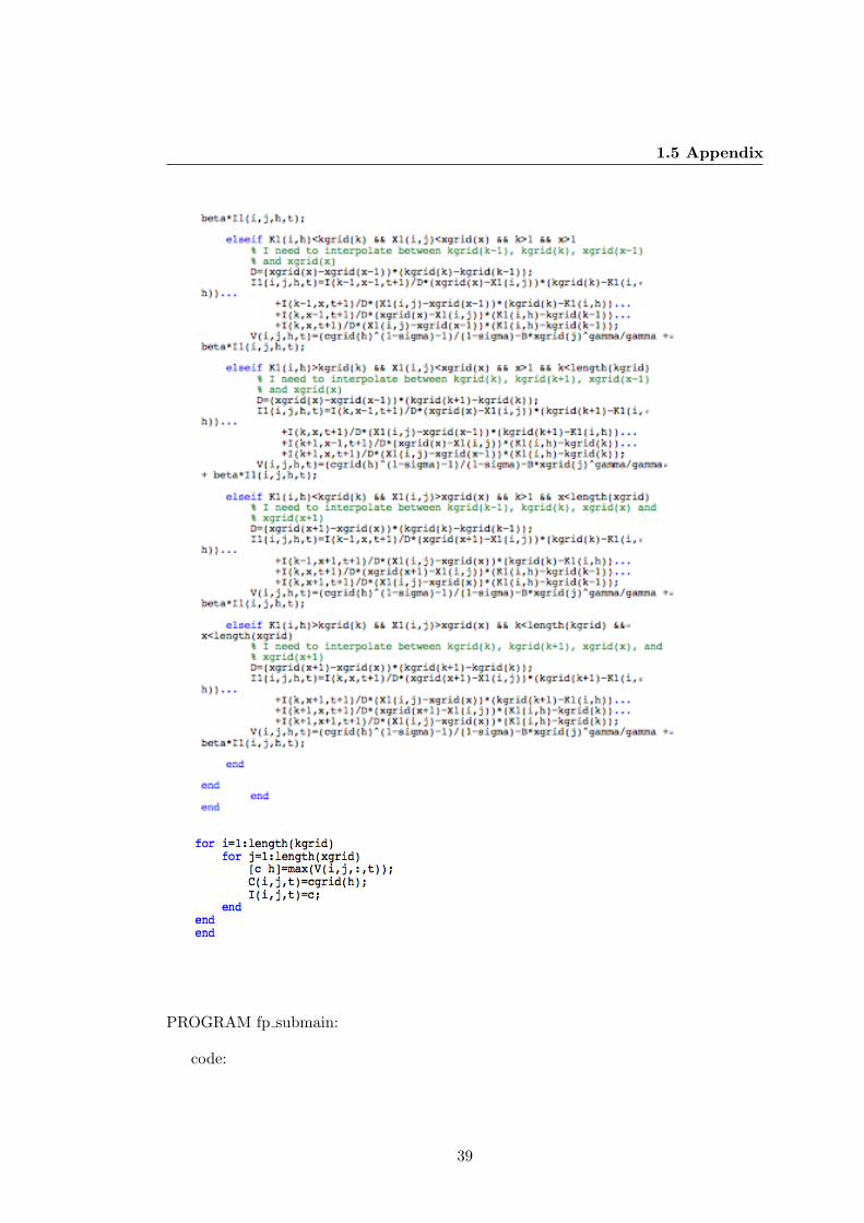
PROGRAM fp submain:
code:
39
1. ON THE NON-OPTIMALITY OF IRREVERSIBLE POLLUTIONACCUMULATION FOR AN INFINITELY LIVED PLANNEDECONOMY.
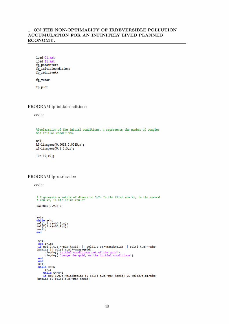
PROGRAM fp initialconditions:
code:
PROGRAM fp retrievekx:
code:
40

1.5 Appendix
41

1. ON THE NON-OPTIMALITY OF IRREVERSIBLE POLLUTIONACCUMULATION FOR AN INFINITELY LIVED PLANNEDECONOMY.
42

1.5 Appendix
PROGRAM fp vstar:
code:
PROGRAM fp plot:
code:
43

1. ON THE NON-OPTIMALITY OF IRREVERSIBLE POLLUTIONACCUMULATION FOR AN INFINITELY LIVED PLANNEDECONOMY.
44

Bibliography
[1] Bellman, Robert, 1957. Dynamic Programming. Princeton N.J., Princeton Univer-
sity Press.
[2] Bellman R., and Dreyfus S., 1962. Applied Dynamic Programming. Princeton N.J.,
Princeton University Press.
[3] Caputo M., 2005. Foundations of Dynamic Economic Analysis. Optimal Control
Theory and Applications. Cambridge University Press.
[4] Dasgupta S., 1982. Control of Resources. Basil Blackwell, Oxford. 3
[5] Dasgupta S., Laplante B., Wang H. and Wheeler D. 2002. “Confronting the Envi-
ronmental Kuznets Curve”, Journal of Economic Perspectives, no.1, Vol. 16, pp.
147-168.
[6] Deissenberg, Ch., Feichtinger, G., Semmler, W., Wirl, F., 2003. Multiple equilibria,
history dependence, and global dynamics in intertemporal optimization models. In:
Barnett, W., Deissenberg, Ch., Feichtinger, G. (Eds.), Economic Complexity: Non-
linear Dynamics, Multi-agents Economies, and Learning, ISETE vol. 14. Elsevier,
Amsterdam, pp. 91-122. 22
[7] Forster, B., 1975. Optimal Pollution Control with a Nonconstant Exponential Rate
of Decay. Journal of Environmental Economics and Management 2, pp. 1-6. 3
[8] Holling C.S., 1973, “Resilience and Stability of Ecological Systems”, Review of
Ecology and Systematics, vol. 4, pp. 1-23. 3
[9] Keeler E., Spence M. and Zeckhauser R. 1972. “The Optimal Control of Pollution”,
Journal of Economic Theory, no. 4, pp. 19-34. 2
45
BIBLIOGRAPHY
[10] Larson, Robert, 1967. A Survey of Dynamic Programming Computational Proce-
dures. IEEE Transaction on Automatic Control, pp. 767-774.
[11] Nordhaus William, 2007. A Review of the Stern Review on the Economics of Cli-
mate Change. Journal of Economic Literature 45, pp. 686-702.
[12] Ryder H.E., and Heal G.M., “Optimal Growth with Intertemporally Dependent
Preferences”, The Review of Economic Studies, Vol. 40, No. 1, pp. 1-31.
[13] Seierstad A. and K. Sydsæter, 1987. Optimal Control Theory with Economic Ap-
plications, North Holland. 30
[14] Stern, Nicholas, 2007. The Economics of Climate Change. The Stern Review. Cam-
bridge and New York, Cambridge University Press. 3
[15] Stokey, Nancy. 1998. “Are There Limits to Growht?”, International Economic Re-
view, No.1, Vol. 39, pp. 1-31. 2, 6
[16] Tahvonen O., and Withagen C., 1996. “Optimality of Irreversible Pollution Accu-
mulation”, Journal of Economic Dynamics and Control, no. 20, pp. 1775-1795. 1,
2
46

2
Is Democracy Good for the
Environment?
Quasi-Experimental Evidence
from Regime Transitions.
Abstract
This paper tests the hypothesis that democratisation is conducive to less environmentaldepletion due to human activity. Using Interrupted Time Series (ITS) design for a panel of47 transition countries and two indexes of pollution, CO2 emissions and PM10 concentrations,I find that democracies and dictatorships have two different targets of environmental quality,with those of democracies higher than those of dictatorships. Income inequality may as wellalter this targets, but with opposite effects in the two different regimes.
JEL Classification: C23, D31, H23, Q58, Q51
Keywords: Democracy; Environment; Cointegration; Interrupted Time Series; Segmented
Regression.
47

2. IS DEMOCRACY GOOD FOR THE ENVIRONMENT?QUASI-EXPERIMENTAL EVIDENCE FROM REGIMETRANSITIONS.
2.1 Introduction
The relation between various measures of pollution and democracy is highly debated.
Two different views about the effect of democracy on the environment have been put
forward: a dominant thinking of the 1970s was that democracy and its associated liber-
ties to pollute, consume and procreate would generate ecological catastrophes, and the
inability of governments to control the “tragedy of the commons” is an evident example
of such a failure of democracies in the management of environmental issues (Desai, (8),
Hardin, (16)). Democracy is also known to be a means for redistributing income and
power to the poor; Rodrik (44) for example, presents evidence that democracy is asso-
ciated with an higher share of wages in GDP and thus lower inequality and Milanovic
(39) finds that democracies with greater inequality of factor income redistribute more
to the poor, so to those whose consumption has an higher marginal impact on the
environment.
At present, however, there is a growing empirical research on the possible affinities
between democracy and ecology. There are several reasons for such a positive rela-
tionship1, basically: i. democracies respect individual rights and so environmentalists
are free to market their ideas and transform them into environmental legislation; ii.
the necessity of democratic government to be elected (or reelected) makes them more
responsive to their citizens; iii. open political systems are more likely to learn from
scientists and other concerned citizens than are autocracies; vi. democratic states tend
to cooperate with each other within international environmental agencies, and finally,
v. because democracies all have free market economies, business in the market can
be subject both to environmental incentives and sanctions (Dasgupta and Maler (6),
Schultz and Crockett (30) and Payne (28)). Furthermore, democracies respect human
life more than autocracies and therefore they are more responsive to life-threatening
environmental degradation (Gleditsh and Sverdrup (13))
In the empirical literature, Bhattarai and Hamming (3), for example, use a measure
of institutional quality (measured by an index of political rights and civil liberties) to
account for the role of different policy regimes in the causes of deforestation in Latin
America, Africa and Asia. Torras and Boyce (34) use a similar technique for a panel
data survey of a variety of air and water pollution indicators. Gallagher and Thacker
1for a systematisation of the argument, see Payne (1995)
48

2.1 Introduction
(12) introduce a concept of “stock of democracy” to study its implications through time.
They all find positive evidence that civil liberties and political rights are associated with
more pro-environmental behaviour.
In this paper, I make use of Interrupted Time Series (ITS) design to study the
effect of democratisation on two indicators of air quality, CO2 emissions and the level
of PM10, in a panel of 47 transition countries during the period 1950-2002 (for CO2)
and 1990-2002 for the other measure. Panel data estimation methods allow control
for unobservable country-specific effects that result in a missing-variable bias in cross-
sectional studies. I included in my sample only transition countries because I believe
it is a natural and transparent way to study the effect of democratisation. The in-
clusion of countries which have not shifted regime may bias the estimate due to the
fact that other events (and not democracy) may be responsible for such a change (like,
for instance, technological progress). This effect may be more easily disentangled in
transition countries due to the possibility of running segmented regressions, as it will
become clearer later.
The method of ITS is a powerful quasi-experimental approach for evaluating the
effects of interventions. Segmented regression analysis of ITS data allows us to as-
sess, in statistical terms, how much an intervention changed an outcome of interest,
immediately and over time, instantly or with delay, and whether factors other than
the intervention could explain the change. If a positive association between democ-
racy and various measure of environmental quality is found in the literature, without
comparing whether different regimes have the opposite effect, nothing can be said, in
principle, about the goodness of that regime in promoting good policies for environ-
mental protection. One example will be illuminating. Suppose we want to study the
effect through time of democracy on the level of CO2 emissions, and suppose we find a
negative and significant effect, so democratic regimes tend to decrease emissions. But
what if also dictatorships reduced them? If that was the case, it would not be possible
to state that democracies are good for the environment, because this would imply that
non-democracies are not, which is not necessarily true. If both democracies and non-
democracies have a positive effect on the environmental quality, it is certainly another
reason that is driving this result.
So, contrary to the other methods commonly used in the literature, this approach
is suitable to measure the effect of democratisation through time, taking into account
49
2. IS DEMOCRACY GOOD FOR THE ENVIRONMENT?QUASI-EXPERIMENTAL EVIDENCE FROM REGIMETRANSITIONS.
of other time-variant effects, and moreover, it is capable of identifying whether other
factors (possibly unknown) are driving the results. Some important observations com-
ing from the empirical evidence are worth considering: due to the fact that income and
democratic institutions are positively correlated (Barro (4), Przeworski and Limongi
(43)), and also that income and cleaner/more efficient technologies are positively corre-
lated (Hausman (21)), cross-country empirical works do not establish causation between
regime and various measures of pollution.
Regressions in panel data are usually done by assuming fixed effect models, which
can solve the issue of accounting for time invariant heterogeneity, and often the dis-
tinction between democracies and others are done by using dummies. This approach
has the pitfall of not disentangling the effects of democracy from other effects in play
during periods of democracy. It is well known that other factors may influence the
performance of a country. In the ideal situation, one could observe the same country
simultaneously under two different types of regime, and this would guarantee that all
the other variables are held constant. But since this is not feasible (what one can ob-
serve is the same country at different points in time), a simple regression, even if it is
able to control for time invariant unobservables, could be biased due to the time vari-
ant unobservable variables. Several effects may cause this bias: History, such as events
which occurred during the period considered providing an alternative explanation of
a given phenomenon, maturation, or processes through which the country produces
changes as a function of time per se (like for example the maturation of technology
towards less energy intensive production processes) or even instability, referred at the
fact that all time series are unstable even when no treatments are applied are all typical
unobservable effects that may bias these estimates.
This paper is organised as follows: section 2.2 motivate the paper, section 2.3
describes the dataset used and some summary statistics, section 2.4 illustrates the
estimation techniques and results, and section 2.5 concludes.
2.2 Motivations
Does democracy really benefit environmental quality? Using a sample of 47 transition
countries, I observe that during the period 1990-2002 the average concentration of PM10
recorded during spells of dictatorship is about 1.36 times bigger than the concentration
50
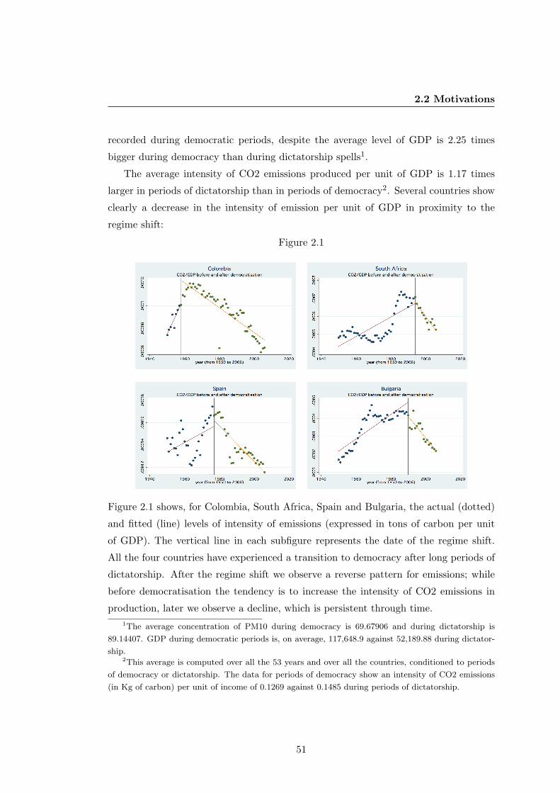
2.2 Motivations
recorded during democratic periods, despite the average level of GDP is 2.25 times
bigger during democracy than during dictatorship spells1.
The average intensity of CO2 emissions produced per unit of GDP is 1.17 times
larger in periods of dictatorship than in periods of democracy2. Several countries show
clearly a decrease in the intensity of emission per unit of GDP in proximity to the
regime shift:
Figure 2.1
Figure 2.1 shows, for Colombia, South Africa, Spain and Bulgaria, the actual (dotted)
and fitted (line) levels of intensity of emissions (expressed in tons of carbon per unit
of GDP). The vertical line in each subfigure represents the date of the regime shift.
All the four countries have experienced a transition to democracy after long periods of
dictatorship. After the regime shift we observe a reverse pattern for emissions; while
before democratisation the tendency is to increase the intensity of CO2 emissions in
production, later we observe a decline, which is persistent through time.1The average concentration of PM10 during democracy is 69.67906 and during dictatorship is
89.14407. GDP during democratic periods is, on average, 117,648.9 against 52,189.88 during dictator-
ship.2This average is computed over all the 53 years and over all the countries, conditioned to periods
of democracy or dictatorship. The data for periods of democracy show an intensity of CO2 emissions
(in Kg of carbon) per unit of income of 0.1269 against 0.1485 during periods of dictatorship.
51
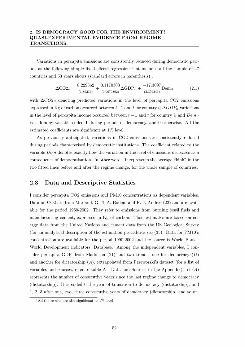
2. IS DEMOCRACY GOOD FOR THE ENVIRONMENT?QUASI-EXPERIMENTAL EVIDENCE FROM REGIMETRANSITIONS.
Variations in percapita emissions are consistently reduced during democratic peri-
ods as the following simple fixed-effects regression that includes all the sample of 47
countries and 53 years shows (standard errors in parenthesis)1:
∆CO2it =8.229862(1.89233)
+0.1170303(0.0079892)
∆GDPit +−17.3097(3.356346)
Demit (2.1)
with ∆CO2it denoting predicted variations in the level of percapita CO2 emissions
expressed in Kg of carbon occurred between t−1 and t for country i, ∆GDPit variations
in the level of percapita income occurred between t− 1 and t for country i, and Demit
is a dummy variable coded 1 during periods of democracy, and 0 otherwise. All the
estimated coefficients are significant at 1% level.
As previously anticipated, variations in CO2 emissions are consistently reduced
during periods characterised by democratic institutions. The coefficient related to the
variable Dem denotes exactly how the variation in the level of emissions decreases as a
consequence of democratisation. In other words, it represents the average “kink” in the
two fitted lines before and after the regime change, for the whole sample of countries.
2.3 Data and Descriptive Statistics
I consider percapita CO2 emissions and PM10 concentrations as dependent variables.
Data on CO2 are from Marland, G., T.A. Boden, and R. J. Andres (22) and are avail-
able for the period 1950-2002. They refer to emissions from burning fossil fuels and
manufacturing cement, expressed in Kg of carbon. Their estimates are based on en-
ergy data from the United Nations and cement data from the US Geological Survey
(for an analytical description of the estimation procedures see (35). Data for PM10’s
concentration are available for the period 1990-2002 and the source is World Bank -
World Development indicators’ Database. Among the independent variables, I con-
sider percapita GDP, from Maddison (21) and two trends, one for democracy (D)
and another for dictatorship (A), extrapolated from Przeworski’s dataset (for a list of
variables and sources, refer to table A - Data and Sources in the Appendix). D (A)
represents the number of consecutive years since the last regime change to democracy
(dictatorship). It is coded 0 the year of transition to democracy (dictatorship), and
1, 2, 3 after one, two, three consecutive years of democracy (dictatorship) and so on.
1All the results are also significant at 1% level
52
2.4 Estimation techniques and results.
During periods of dictatorship (democracy) it is coded zero. The last independent
variable used is Inequality, from the EHII dataset of the University of Texas Inequality
Project (UTIP). This measure is an estimate of the Theil’s index of household’s in-
come inequality derived from econometric relationships between UTP-UNIDO (dataset
that calculates the industrial pay inequality measures based on the UNIDO Industrial
statistics), other conditioning variables, and the World Bank’s Deninger and Squire
Dataset1.
Table B in the appendix lists all the countries included in the sample, and their re-
spective regime changes to and from democracy. They are mainly developing countries,
with the exception of the countries distinguished by an asterisk which are considered
by IMF (World Economic Outlook updated to april 2009) developed or advanced. The
following table 1 shows the summary statistics of the primary explanatory variables:
2.4 Estimation techniques and results.
2.4.1 Diagnostic tests and model selection
The first step to decide the best way to estimate a relationship of interest, is to choose
the appropriate econometric tool. In order to do so, it is necessary to verify the char-
acteristics of the data generating processes, by testing for eventual unit root. I test
the occurrence of unit root on the series percapita CO2 emissions, percapita GDP,
PM10 concentrations and inequality using four tests for panel data: Levin, Lin and
Chu (LLC), Im, Pesaran and Shin (IPS), ADF and PP-Fisher tests. All these tests
suggest that the data generating processes of CO2 emissions and GDP have unit root,
while PM10 concentration and inequality appear stationary2.
For what concerns the dependent variable PM10, given its stationarity, it cannot be
cointegrated with any other variable and therefore a standard Least Squares Dummy
Variable (LSDV) model for testing the effects of democracy on its level is appropriate,
as it should produce stationary (possibly normal) residuals.
For what concerns instead the model for CO2 emissions, I cannot say a priori if
the same LSDV model is appropriate, and a test for cointegration is mandatory so to
1For a detailed presentation of the techniques used to construct such an index, visit the University
of Texas’ website at http://utip.gov.utexas.edu/default.html2For a detailed description of these tests, the tests that will follow and results, refer to the appendix.
53

2. IS DEMOCRACY GOOD FOR THE ENVIRONMENT?QUASI-EXPERIMENTAL EVIDENCE FROM REGIMETRANSITIONS.
Table 2.1: Summary statistics of the primary explanatory variables
Variable Description Obs mean Std.Dev. min max
CO2 Kg of carbon per-capita
2255 563.663 834.6266 0 4470
PM10 Concentrations ofparticulate mat-ters, microgramsper cubic meter
611 72.10575 48.19759 11.9218 274.45
GDP Percapita GDP,1990$
2452 2778.26 2677.37 289.15 16572.83
Dem Dummy forDemocracy(Przeworski)
2234 .3531782 .4780645 0 1
D Trend for Dem 2234 3.176813 6.653377 0 44A Trend for (1-
Dem)2234 10.27261 12.0507 0 50
Ineq Household’s in-come inequality(UTIP)
1129 42.00001 6.666231 19.81 62.32
D ·INEQ
Product of in-equality andthe trend fordemocracy
1124 160.2534 323.7205 0 1857.66
A ·INEQ
Product of in-equality andthe trend forautocracy
1124 491.798 544.5511 0 2232.621
Y ear Year (from 1950to 2002)
2491 1976 15.30013 1950 2002
N 2491
54

2.4 Estimation techniques and results.
exclude possible problems related to spurious regression1. If indeed the two series were
cointegrated, standard OLS techniques would produce superconsistent estimates of the
parameters, but if they were not, the model would suffer of the spurious regression
problem with invalid inference of the parameters of interest.
In the Engle-Granger approach, cointegration is tested by verifying that the resid-
ual series generated by the regression of one I(1) variable over another I(1) variable
is stationary2. To verify whether percapita CO2 emissions and percapita GDP are
cointegrated, I use the approach suggested by Kao (27). The global ADF statistic
for Kao residual cointegration test with the null of no cointegration shows a t-stat of
3.499820 with a p-value of 0.0002, so this test strongly suggests that those two series
are cointegrated.
Maddala and Wu (32) combined tests from individual cross-sections (trace and
maximum eigenvalue tests) reject the hypothesis of absence of cointegration at 1% level,
and, as expected, accept the hypothesis that there exists one cointegrating relation3.
So, substantial evidence points out that a cointegrating relation between emissions and
income exists, so the use of a procedure that takes into account this fact is justified.
The choice of estimating the model using a single equation or a Vector Error Cor-
rection Model (VECM) is made by testing for weak exogeneity of the variables on the
right-hand side of the equation describing the long run relationship of CO2 with GDP.
Estimating with a single equation when the variables are not weakly exogenous is po-
tentially inefficient and it does not lead to the smallest variance against alternatives,
because information is lost. Using the approach suggested by Urbain (48), I test weak
exogeneity by testing whether the error correction term embedded in the short run
ECM4 is significant in the equation determining ∆GDPit. In particular, weak exogene-
ity requires that ∆GDPit does not depend on disequilibrium changes represented by1Spurious regressions occur whenever one regresses a nonstationary variable over another non-
stationary variable which are not cointegrated. In general, the estimated coefficients appear to be
significant but they lack any real and plausible correlation, since what is correlated is just a common
trend and nothing else. Under a spurious regression, the tendency of both series to be growing is picked
up by the regression model, even though each series is growing for very different reasons and at a rates
which are uncorrelated, and produce nonstationary residuals.2Since in my dataset there are only two nonstationary variables, it follows that at most one coin-
tegrating relation may exist.3In performing these tests, it’s been assumed that there is no deterministic trend.4εit−1 is computed as a residual of the long run relationship explaining percapita CO2 emissions.
55

2. IS DEMOCRACY GOOD FOR THE ENVIRONMENT?QUASI-EXPERIMENTAL EVIDENCE FROM REGIMETRANSITIONS.
εit−1. Results of this test, deeply detailed in the appendix, show that GDP is weakly
exogenous so the estimation of the model for CO2 emissions using a simple equation
approach is suitable for my purpose.
2.4.2 Interrupted Time Series
Interrupted time series (ITS) are a powerful quasi-experimental approach for evaluat-
ing the effects of interventions. Segmented regression analysis of ITS data allows to
assess, in statistical terms, how much an intervention changed an outcome of interest,
immediately and over time, instantly or with delay, and whether factors other than the
intervention could explain the change. In this paper, I make use of this ITS design to
estimate the effects of democratisation on the level of emissions produced, in a panel
of 47 countries for the period 1950-2002 for CO2 and 1990-2002 for PM10. For each
country in my sample, the levels of emissions and concentration of particulate matters,
real percapita incomes and the regime are measured at regularly spaced intervals over
time. To determine the effect of a regime change on the level of the two indexes of pol-
lution, I generate two series (namely, D and A representing the number of consecutive
years since the last regime change to, respectively, democracy and dictatorship) which
are divided into two or more segments at changing points, when the regime type varies.
So, if a country, at a given date, has shifted from dictatorship to democracy, and there
is only one shift in the period taken into consideration, then the time series is divided
into two segments. If the number of shifts is n, the number of segment will be, in
general, n+1. In detail, D and A are trend variables which are evaluated progressively
according to the age of the democracy or autocracy. The advantage of using those
two variables is that they allow assessment of the effect of the regime through time as
well whether other effects may explain the change. If indeed the coefficients relative
to those trends have the same sign, this methods allows to conclude that other factors
(like general technological progress) may have played a major role in the determination
of the environmental policy, and not the regime.
2.4.3 Econometric specifications and results
Due to the nature of data generating process of my variables of interest, I have to
specify two different models for estimating the effect of the regime on CO2 and on
the level of PM10 concentrations. Previous tests for cointegration between CO2 and
56
2.4 Estimation techniques and results.
GDP suggest that those two variables have a long run relationship; they move closely
together over time and their difference is stable. Test for weak exogeneity shows that
GDP is weakly exogenous with respect to CO2 so cointegration approaches which use
a single equation are appropriate and no loss of information (and efficiency) occur. For
estimating the effect of the regime on the level of CO2 emission, then, I will use the
procedure proposed by Engle and Granger (12). The Engle-Granger Error Correction
Model (ECM) is appropriate in this setting and has the advantage of incorporating both
long run and short run effects; if the model is in disequilibrium the ECM will provide
information on the speed of adjustment to equilibrium. Moreover, all the terms in the
model are stationary, and so standard regression techniques are valid, and finally, the
fact that CO2 and GDP are cointegrated of order CI(1,1) implies that an ECM exists
(and, conversely, an ECM generates cointegrated series) and so ECM is immune from
the spurious regression problem1.
For what concerns the estimation of the effects of the two different regimes on the
level of PM10 concentrations, I use a LSDV model to take into account of country
specific fixed effects, and since tests for unit root for the PM10 series show that it is
stationary, standard OLS procedures can be applied. In both econometric specifications
I introduce two different trends, or, more precisely, two interrupted series of trends, D
and A, which represent, respectively, the number of consecutive years since the last
democratisation or autocratisation. During periods of dictatorship, D is coded zero,
and during periods of democracy, A is coded zero. In this setup, D and A represent
the effect through time on emissions or on concentration of pollution of the type of
regime. The other independent variables included in the model are inequality and
the cross effects of inequality with the two trends for regime. The reason for their
inclusion is that depending on who is the decisive political actor in the two different
regimes, inequality may have different effects. So, on one hand, when the population as
a whole is involved in the decision process (through the electoral mechanism), different
levels of income inequality change the median voter’s wealth and so the perceived
value of income (or consumption) relative to the environmental quality, and therefore
inequality is expected to worsen the environmental quality. On the other hand, during
1This can be referred to Granger’s representation theorem for dynamic modelling, in Engle and
Granger (12)
57

2. IS DEMOCRACY GOOD FOR THE ENVIRONMENT?QUASI-EXPERIMENTAL EVIDENCE FROM REGIMETRANSITIONS.
autocratic periods, if increased inequality is in favor of the dictator1, it could increase
environmental quality, since the rich dictator values the environment more, compared
to consumption.
In order to estimate the relation between different regimes and CO2 emissions,
consider the following ARDL(1,1)
CO2it = α0i + γ1CO2it−1 +n∑j=1
δ0jXjit +n∑j=1
δ1jXjit−1 +
+4∑z=3
δ2zX4itXzit +4∑z=3
δ3zX4it−1Xzit−1 + εit (2.2)
with j = 1, ..., 4 and
X1 = GDP
X2 = D
X3 = A
X4 = INEQ
with some manipulations (shown in appendix) we end up with the usual ECM:
∆CO2it =n∑j=1
δ0j∆Xjit +3∑z=2
δ2zWz − (1− γ1)[CO2it−1 −
α0i
1− γ1−
−n∑j=1
δ0j + δ1j
1− γ1Xjit−1 −
3∑z=2
δ2z + δ3z
1− γ1X4it−1Xzit−1
]+ ηit (2.3)
Wz =(X4it∆Xzit + ∆X4itXzit −∆X4it∆Xzit
)(2.4)
1It is indeed well known that many countries in Africa and the Caribbean suffer and have suffered
from “kleptocratic” regimes (Acemoglu, Robinson and Verdier, (1)) run by individulas who use their
power to transfer a large fraction of society’s resources to themselves. Two of the most “kleptocratic
successes” are those of Mubutu Sese Seko in the Democratic Republic of Congo (Zaire) and Rafael
Trujillo in the Dominican Republic. To have an idea of the numbers, in the 70’s, 15-20% of Congo’s
operating budget went directly to Mubutu, and in 1977 Mubutu’s family took $71 million from the
National Bank for personal use and in the 80’s his personal fortune was estimated in $5 billion (Leslie,
(20), p. 72). In the Dominican Republic, Trujillo became in power after he elected himself in a
fraudulent election and at the end of his regime, the fortune of Trujillo’s family amounted to about
100% of GDP at current prices and the family “controlled almost 80% of the country’s industrial
production” (Moya Pons, (25), p. 398). Other examples of “keptocratic regimes” include Haiti under
the Duvaliers, Nicaragua under the Somozas, Uganda under Idi Amin, Liberia under Charles Taylor
and the Philippines under Ferdinand Marcos, but the list can go on, if we include less extreme cases.
58

2.4 Estimation techniques and results.
where the expression in square brackets represents the long run relationship between
CO2 and GDP. If the model is in equilibrium, this expression is equal to zero, and if it is
not, the coefficient −(1−γ1) represents the speed of adjustment toward it. Therefore, I
first estimate the long run relationship between CO2 and the other covariates as follows:
CO2it = β0i + β1GDPit + β2Dit + β3Ait + β4INEQit +
+ β5Dit · INEQit + β6Ait · INEQit + εit (2.5)
with
βj =δ0j + δ1j
1− γ1j = 1, ..., 4
βh =δ2h + δ3h
1− γ1h = 5, 6
using a standar LSDV to account for specific, country-level time invariant effects (whose
coefficient is represented by β0i) and using cluster-robust standard errors. The results
of this estimation are shown in table 2. The second step is to estimate the residuals
from equation 2.5 and proceed to the estimation of the unrestricted error correction
model
∆CO2it = δ01∆GDPit + δ02∆D∗it + δ03∆A∗it + δ04INEQ+
+ δ22WDit + δ23WAit − (1− γ1)εit−1 + ηit (2.6)
where WDit and WAit are defined as:
WDit = Dit ·∆INEQit + ∆D∗it · INEQit −∆D∗it ·∆INEQit
WAit = Ait ·∆INEQit + ∆A∗it · INEQit −∆A∗it ·∆INEQit
and εit−1 is
εit−1 = CO2it−1 − β0i − β1GDPit−1 − β2Dit−1 − β3Ait−1 +
− β4INEQit−1 − β5Dit−1 · INEQit−1 − β6Ait−1 · INEQit−1
Results of the estimation of equation 2.6 are shown in table 3. Table F in the appendix
shows the coefficients relative to the fixed effects estimated in equation 2.5.
As previously written, the series PM10 is stationary and therefore there cannot
exist any cointegrating relation. It follows that a simple LSDV model is appropriate
59

2. IS DEMOCRACY GOOD FOR THE ENVIRONMENT?QUASI-EXPERIMENTAL EVIDENCE FROM REGIMETRANSITIONS.
to estimate the effects of the regime, since the residuals are expected to be stationary
(results of the tests of unit root on the residuals are shown in the appendix). In order
to conform to the EKC literature, I estimate the following equation including among
the regressors also the square and cubic powers of GDP1:
PM10it = β0i + β1GDPit + β2GDP2it + β3GDP
3it + β4Dit + β5Ait +
+ β6INEQit + β7Dit · INEQit + β8Ait · INEQit + εit (2.7)
and the results are shown in table 2.
As it is possible to see, the trends for democracy and dictatorship have, respec-
tively, a negative effect on the level of emissions/pollution, in both models and all the
coefficients (except that relative to inequality for the model of CO2 emissions) are sta-
tistically significant at the standard 5% level. For model 1 (PM10), the elasticity of the
concentration of PM10 with respect to one year increase in democracy (∂PM10/∂D),
computed at the mean of inequality is equal to -2.15, and the same elasticity computed
for one year increase in dictatorship (∂PM10/∂A) is 0.1192. For the second model,
relative to CO2 emissions, ∂CO2/∂D = -1.267 and ∂CO2/∂A=4.102. It is possible to
say therefore that in both models (even in the second all the conclusions apply only to
the long run period) democracy is good for the environment, and moreover the argu-
ment is reinforced by the fact that non-democracies are not. Table 3 shows the results
from the estimation of the unrestricted ECM for CO2 emissions:
The main results are reported in table 3. Variations in the level of CO2 are, of
course, positively related to variations in global production, and the coefficient attached
to ε represents the speed of adjustment towards the equilibrium. It is worth noting
that the coefficient related to ∆D∗it is not significant at the standard 5% level (in fact,
it has a p-value of 0.574), while the coefficient related to the variation in the trend
for dictatorship is positive and significatively related to increases in the variation of
emissions. This effect may be the cause of the slower reactions of democracies with
respect to autocracies. Democracies are indeed constrained by consultations, elections,
every decisions has often to pass the evaluations of another independent organism, and
this procedure takes time. On the contrary, in dictatorship the decisions are taken by
one individual only and they have not to be scrutinised by other independent powers.1It is important to notice that the sign and the significancy of the other covariates remains un-
changed if those two terms are excluded from the model.
60

2.4 Estimation techniques and results.
Table 2.2: Results of the estimation of the model for PM10 and the long run equilibriumrelationship for CO2
(1) (2)PM10 Percapita CO2
Percapita GDP 0.00375∗∗ 0.163∗∗∗
(3.32) (29.39)
D -4.254∗∗∗ -33.41∗
(-4.59) (-2.28)
A 1.091∗ 36.96∗∗∗
(2.18) (9.23)
INEQ -0.310∗ -0.576(-2.01) (-0.22)
D · INEQ 0.0500∗∗ 0.764∗
(2.73) (2.37)
A · INEQ -0.0231∗ -0.781∗∗∗
(-2.12) (-8.63)
r2 0.345 0.703N 316 1110
t statistics in parentheses
∗ p < 0.05, ∗∗ p < 0.01, ∗∗∗ p < 0.001
61
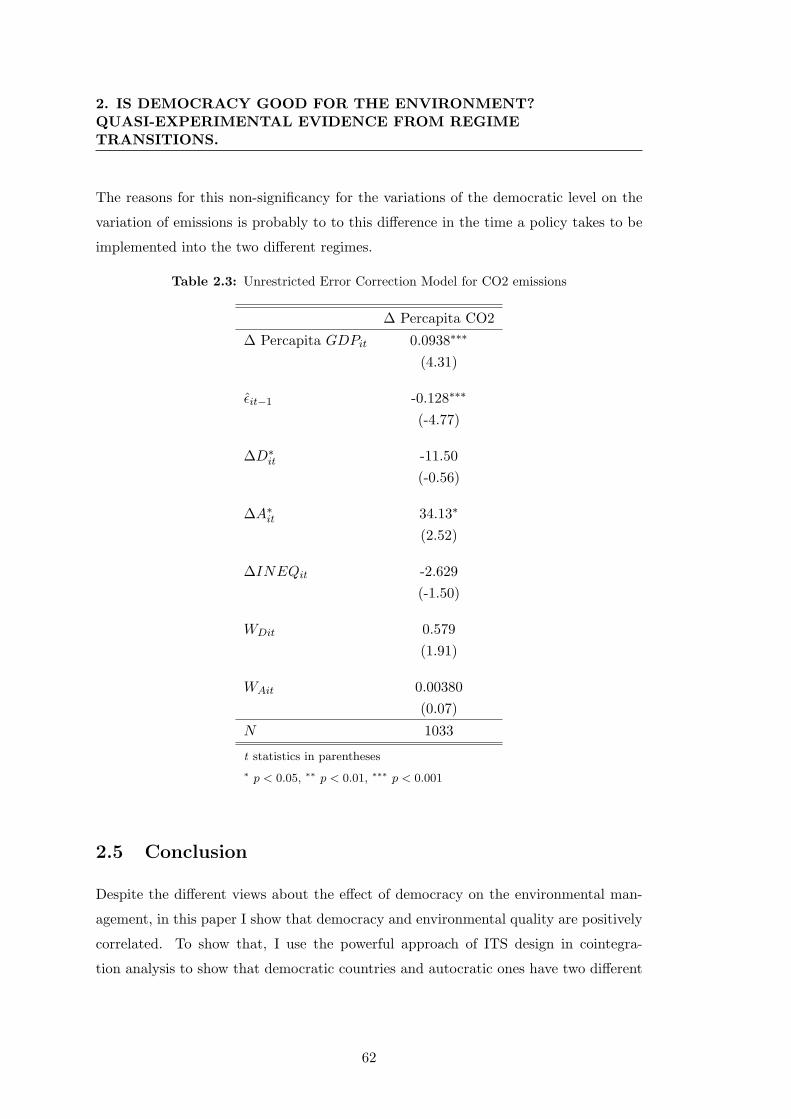
2. IS DEMOCRACY GOOD FOR THE ENVIRONMENT?QUASI-EXPERIMENTAL EVIDENCE FROM REGIMETRANSITIONS.
The reasons for this non-significancy for the variations of the democratic level on the
variation of emissions is probably to to this difference in the time a policy takes to be
implemented into the two different regimes.
Table 2.3: Unrestricted Error Correction Model for CO2 emissions
∆ Percapita CO2
∆ Percapita GDPit 0.0938∗∗∗
(4.31)
εit−1 -0.128∗∗∗
(-4.77)
∆D∗it -11.50(-0.56)
∆A∗it 34.13∗
(2.52)
∆INEQit -2.629(-1.50)
WDit 0.579(1.91)
WAit 0.00380(0.07)
N 1033
t statistics in parentheses
∗ p < 0.05, ∗∗ p < 0.01, ∗∗∗ p < 0.001
2.5 Conclusion
Despite the different views about the effect of democracy on the environmental man-
agement, in this paper I show that democracy and environmental quality are positively
correlated. To show that, I use the powerful approach of ITS design in cointegra-
tion analysis to show that democratic countries and autocratic ones have two different
62

2.6 Appendix
targets of environmental quality, with those for democracy higher than those for au-
tocracies. Previous works on democracy and environmental quality were indeed unable
to assert that democracy is really good for the environment because they did not show
that non-democracies are not. Segmented regression analysis of ITS allows not only to
see the effect of democracy through time, but also if this effect differs from the effect
of autocracy. The weakness of the previous works in this field was therefore that not
comparing the results with those for dictatorships, the positive effect of democracy on
the environment might not be due to democracy per se, but from other effects, like
maturation, or technological progress, common to both regimes. In this panel of 47
transition countries, this approach shows that democratisation is consistently associ-
ated to a reduction of CO2 emissions and PM10 concentrations, but this process may
be quite slow because - at least in the ECM relative to CO2 emissions - it is detectable
only in the long run. Due to the fact that democratic institutions tend to be slower
than autocratic ones in taking decisions and acting, in the short run we do not observe
a negative effect of democracy on the level of emissions, while the positive effect of
dictatorship is quite consistent. Inequality has two different effects depending on the
incumbent regime: in any case it counterbalances the global effect of the regime. In
democracy, increased inequality means that the decisive citizen is poorer and so less
willing to pay for environmental protection, while inequality during periods of autoc-
racy, under the assumption that this inequality favor the dictator at the expense of the
rest of the citizens, it may retain the negative effect of the regime since it increases the
dictator’s income and so it increases his demand for environmental quality. The overall
effect, however, is that dictatorships tend to be associated to a worse environment than
democracies.
2.6 Appendix
Diagnostic tests
Panel Unit root test
The first step to decide the best way to estimate a relationship of interest, is to choose
the appropriate econometric tool. In order to do so, it is necessary to verify the char-
acteristics of the data generating processes: for each nondeterministic series (CO2
emissions, percapita GDP, PM10 concentrations and Inequality), I test whether they
63

2. IS DEMOCRACY GOOD FOR THE ENVIRONMENT?QUASI-EXPERIMENTAL EVIDENCE FROM REGIMETRANSITIONS.
have stationary mean and variance. Available tests for unit root on panel data are
based on the Dickey Fuller test (or its augmented version), so I test the following:
yit = ρiyit−1 +X ′itδi + εit (2.8)
with i = 1, ..., N and t = 1, ..., Ti. ρi represents the autoregressive coefficient for country
i, Xit is matrix representing the exogenous variables in the model, including any fixed
effects and individual trends and εit are the errors which are assumed i.i.d.. If |ρi| = 1,
then yi contains a unit root. For practical purpose, the tests for unit root are performed
using the following basic ADF specification:
∆yit = αiyit−1 +pi∑j=1
βij∆yit−j +X ′itδi + εit (2.9)
with αi = ρi − 1.
Levin, Lin and Chu test assumes that the unit root process is common to all the
cross sections so it assumes αi = α for every i. The test is performed by testing the
null hypothesis H0 : α = 0 against the alternative H1 : α < 0 for all the cross section
units. Their procedure derives estimates of α from proxies for ∆yit and yit that are
standardised and free of autocorrelation and deterministic components. For a given set
of lag orders pi, their procedure begins by estimating two additional sets of equations,
∆yit =pi∑j=1
βij∆yit−j +X ′itδ (2.10)
yit =pi∑j=1
βij∆yit−j +X ′itδ (2.11)
and denoting (β, δ) the estimated coefficients of equation 2.10 and (β, δ) those of equa-
tion 2.11. They define, then, ∆yit and yit−1 by taking, respectively, ∆yit and yit−1
and removing the autocorrelations and deterministic components using their respective
auxiliary estimates
∆yit = ∆yit −pi∑j=1
βij∆yit−j −X ′itδ (2.12)
yit−1 = yit−1 −pi∑j=1
βij∆yit−j −X ′itδ (2.13)
64

2.6 Appendix
and standardise both ∆yit and yit−1 by dividing by the regression standard error
∆yit =∆yitsi
yit−1 =yit−1
si
where si are the estimated standard errors from estimating each ADF in equation 2.9.
The estimate of α is then obtained from the pooled proxy equation
∆yit = αyit−1 + ηit (2.14)
which, under the null, a modified t-statistics for the resulting α is asymptotically nor-
mally distributed
t∗α =tα − (NT )SN σ−2se(α)µmT ∗
σmT ∗→ N(0, 1)
where tα is the standard statistic for α = 0, σ2 is the estimated variance of the error
term η, se(α) is the standard error of α, and
T = T − (∑i
pi/N)− 1,
SN is the mean of the ratios of the long run standard deviation for each individual, and
it is estimated using kernel-based techniques, and µmT ∗ and σmT ∗ are adjustment terms
for the mean and standard deviation (for more details, refer to the original article of
Levin, Lin and Chu (29)). In order to perform this test, I include individual constant
terms (fixed effects), and an individual trend, so my Xit matrix is a 2NTx2N matrix,
where the first NTxN block is a matrix of dummy variables, each representing one
single country, and the other block going from row NT + 1 to 2NT and from column
N + 1 to 2N is a matrix of trends, one for each single countries. All the other terms in
the matrix are equal to zero.
If the test for common unit root fails, it might be convenient to check whether
individual unit root exists. Tests available for that are Im, Peasaran and Shin, Fisher
AD and PP tests. Im, Pesaran and Shin test begin by specifying a separate ADF
regression for each cross-section according to equation 2.9 with the null
H0 : αi = 0 for every i = 1, 2, ..., N
65

2. IS DEMOCRACY GOOD FOR THE ENVIRONMENT?QUASI-EXPERIMENTAL EVIDENCE FROM REGIMETRANSITIONS.
and the alternative hypothesis is
H1 :αi = 0 for i = 1, 2, ..., N1
αi < 0 for i = N1 + 1, N1 + 2, ..., N
That can be interpreted as a nonzero fraction of the individual processes is stationary.
After having estimated the separate ADF regressions, the average of the t-statistics for
αi from the individual ADF regressions, tiTi(pi),
tNT =( N∑i=1
tiTi(pi))/N
is adjusted to arrive to the desired statistics. Critical values are provided in the Im,
Pesaran and Shin’s paper (25) for different number of cross sections and time periods
when pi = 0 for all i, but in the general case when the lag order in equation 2.9 may
be nonzero for some cross-sections, they show that a properly standardised tNT has an
asymptotic standard normal distribution
WtNT −
√N(tNT −N−1
∑Ni=1E(tiT (pi))
)√N−1
∑Ni=1 V ar(tiT (pi))
→ N(0, 1)
and the expression for the expected mean and variance of the ADF regression t-
statistics, E(tiT (pi)) and V ar(tiT (pi)) are provided by Im, Pesaran and Shin for various
values of T and p and different test equation assumptions. I will use, in this paper, one
lag and, as deterministic component, an individual constant, without introducing any
trend term. Finally, there are other two tests for checking individual unit root: Fisher
ADF and Fisher PP tests, which are based upon the idea by Maddala, Wu and Choi,
and combine the p-values from individual unit root tests. They work as follows: define
πi the p-value from individual unit root test for cross-section i, then under the null of
unit root for all the N cross sections, we have the asymptotic result that
−2N∑i=1
log(πi)→ χ22N
and also, Choi demonstrates that
Z =1√N
N∑i=1
Φ−1(πi)→ N(0, 1)
66

2.6 Appendix
where Φ−1 is the inverse of a standard normal cumulative distribution function. For
both the Fisher tests, I specify as exogenous variables an individual constant (fixed
effect) and an individual time trend.
Table C in this appendix shows the results of the tests for all the nondeterministic
series. These tests accept the hypothesis of unit root only for two out of four series,
percapita GDP and percapita CO2 emissions. Since the level of concentration of partic-
ulate matters (PM10) is stationary, it cannot be cointegrated with any other variable,
while in principle CO2 and GDP could be. For what concerns the dependent variable
PM10, then, a standard Least Squares Dummy Variables (LSDV) model for testing
the effect of democracy on its level it is appropriate, as it should produce stationary
(possibly normal) residuals. For what concerns the model for CO2 emissions, we cannot
say a priori whether the same LSDV model is appropriate, and a test for cointegration
is mandatory. If indeed the two series were cointegrated, that model would produce
superconsistent estimates of the parameters, but if they were not, the model would
suffer of the problem of the spurious regression with invalid inference of the parameters
of interest. In this case, the tendency of both series to be growing leads to correla-
tion which is picked up by the regression model, even though each series is growing
for very different reasons and at a rates which are uncorrelated. Thus, in absence of
cointegration (which will be tested in the next subsection) correlation between non-
stationary series does not imply the kind of causal relationship that might be inferred
from stationary series, so standard estimation techniques like OLS cannot be used.
Panel cointegration test
If two or more variables are nonstationary or I(1), if they are not cointegrated, the
residual series obtained by regressing one I(1) variable over another I(1) variable is
expected to be nonstationary, or I(1). This would lead to spurious regression since the
estimated coefficients do not reflect a real relationship between those two variables,
but simply correlated time trends. This however would be different if those two vari-
ables were cointegrated, and the coefficients would benefit from the “superconsistency”
property. Since in my dataset there are only two nonstationary variables, namely, CO2
and GDP, it follows that at most one cointegrating relation may exist. In the Engle-
Granger approach, cointegration is tested by verifying that the residual series generated
by the regression of one I(1) variable over another I(1) variable is stationary. To verify
67

2. IS DEMOCRACY GOOD FOR THE ENVIRONMENT?QUASI-EXPERIMENTAL EVIDENCE FROM REGIMETRANSITIONS.
whether percapita CO2 emissions and percapita GDP are cointegrated, I use the ap-
proach suggested by Kao (27). Kao uses a two-step procedure to test for cointegration:
in the first step, he regress the dependent variable (which is I(1)) over the independent
(also I(1)) specifying cross-section specific intercepts and homogeneous coefficient: he
basically regresses
CO2it = X ′itαi + βGDPit + eit (2.15)
where Xit is a matrix of dummy variables representing each single country and assuming
CO2it = CO2it−1 + uit and GDPit = GDPit−1 + εit for t = 1, ..., T and i = 1, ..., N .
Then Kao runs the pooled auxiliary regression
eit = ρeit−1 +p∑j=1
ψj∆eit−j + vit (2.16)
Assuming p = 11, this augmented Dikey Fuller test for panel data reject at 1% level the
hypothesis that ρ = 1. The global ADF t-statistic for Kao residual cointegration test
with the null hypothesis of no cointegration shows a t-stat of 3.499820 with a p-value
of 0.0002, so this test strongly suggests that those two series are cointegrated (detailed
results of this test are in this appendix - table D).
Maddala and Wu (32) combined test from individual cross-sections2 is specified as
follows: consider the following VAR representation for each cross-section unit:
Yt = A1Yt−1 +A2Yt−2 + εt (2.17)
where Y is a vector of I(1) variables (in my case, CO2 and GDP). Subtracting Yt−1 on
the left and right hand side of equation 2.17 and adding and subtracting A2Yt−1 from
the right hand side, we get
∆Yt = ΠYt−1 + Γ∆Yt−1 + εt (2.18)
with Π = (A1 + A2 − I) and Γ = −A2. Granger’s representation theorem asserts that
if the coefficient matrix Π has a reduced rank r < k, then there exists kxr matrices
α and β each with rank r such that Π = α · β′ and β′Yt is I(0). r is the number
of cointegrating relations and each column of β is the cointegrating vector, and the
elements of α are known as the adjustment parameters in the VEC model. Johansen’s1Similar results are obtained for longer lags specifications, up to four.2Maddala and Wu use the results obtained by Fisher and Johansen (14)
68
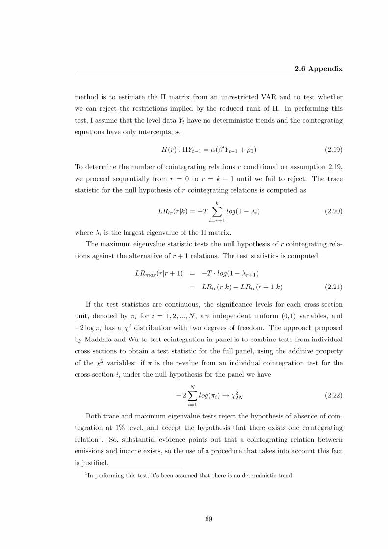
2.6 Appendix
method is to estimate the Π matrix from an unrestricted VAR and to test whether
we can reject the restrictions implied by the reduced rank of Π. In performing this
test, I assume that the level data Yt have no deterministic trends and the cointegrating
equations have only interceipts, so
H(r) : ΠYt−1 = α(β′Yt−1 + ρ0) (2.19)
To determine the number of cointegrating relations r conditional on assumption 2.19,
we proceed sequentially from r = 0 to r = k − 1 until we fail to reject. The trace
statistic for the null hypothesis of r cointegrating relations is computed as
LRtr(r|k) = −Tk∑
i=r+1
log(1− λi) (2.20)
where λi is the largest eigenvalue of the Π matrix.
The maximum eigenvalue statistic tests the null hypothesis of r cointegrating rela-
tions against the alternative of r + 1 relations. The test statistics is computed
LRmax(r|r + 1) = −T · log(1− λr+1)
= LRtr(r|k)− LRtr(r + 1|k) (2.21)
If the test statistics are continuous, the significance levels for each cross-section
unit, denoted by πi for i = 1, 2, ..., N , are independent uniform (0,1) variables, and
−2 log πi has a χ2 distribution with two degrees of freedom. The approach proposed
by Maddala and Wu to test cointegration in panel is to combine tests from individual
cross sections to obtain a test statistic for the full panel, using the additive property
of the χ2 variables: if π is the p-value from an individual cointegration test for the
cross-section i, under the null hypothesis for the panel we have
− 2N∑i=1
log(πi)→ χ22N (2.22)
Both trace and maximum eigenvalue tests reject the hypothesis of absence of coin-
tegration at 1% level, and accept the hypothesis that there exists one cointegrating
relation1. So, substantial evidence points out that a cointegrating relation between
emissions and income exists, so the use of a procedure that takes into account this fact
is justified.1In performing this test, it’s been assumed that there is no deterministic trend
69
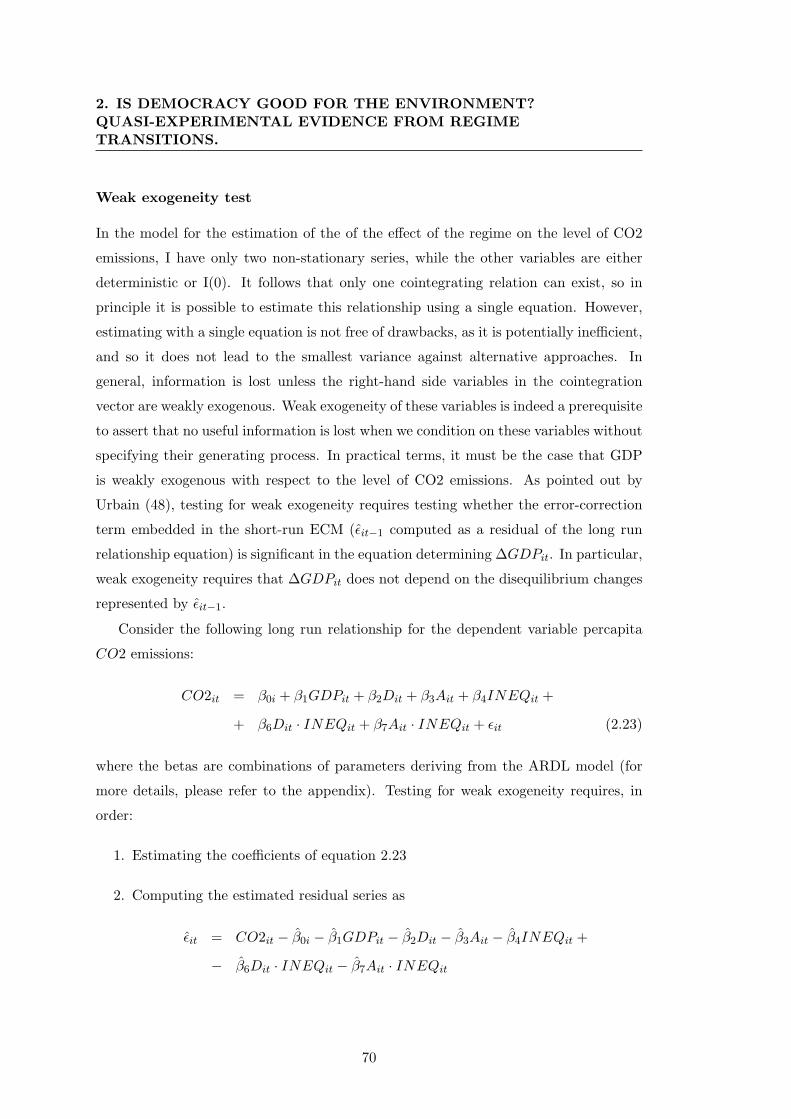
2. IS DEMOCRACY GOOD FOR THE ENVIRONMENT?QUASI-EXPERIMENTAL EVIDENCE FROM REGIMETRANSITIONS.
Weak exogeneity test
In the model for the estimation of the of the effect of the regime on the level of CO2
emissions, I have only two non-stationary series, while the other variables are either
deterministic or I(0). It follows that only one cointegrating relation can exist, so in
principle it is possible to estimate this relationship using a single equation. However,
estimating with a single equation is not free of drawbacks, as it is potentially inefficient,
and so it does not lead to the smallest variance against alternative approaches. In
general, information is lost unless the right-hand side variables in the cointegration
vector are weakly exogenous. Weak exogeneity of these variables is indeed a prerequisite
to assert that no useful information is lost when we condition on these variables without
specifying their generating process. In practical terms, it must be the case that GDP
is weakly exogenous with respect to the level of CO2 emissions. As pointed out by
Urbain (48), testing for weak exogeneity requires testing whether the error-correction
term embedded in the short-run ECM (εit−1 computed as a residual of the long run
relationship equation) is significant in the equation determining ∆GDPit. In particular,
weak exogeneity requires that ∆GDPit does not depend on the disequilibrium changes
represented by εit−1.
Consider the following long run relationship for the dependent variable percapita
CO2 emissions:
CO2it = β0i + β1GDPit + β2Dit + β3Ait + β4INEQit +
+ β6Dit · INEQit + β7Ait · INEQit + εit (2.23)
where the betas are combinations of parameters deriving from the ARDL model (for
more details, please refer to the appendix). Testing for weak exogeneity requires, in
order:
1. Estimating the coefficients of equation 2.23
2. Computing the estimated residual series as
εit = CO2it − β0i − β1GDPit − β2Dit − β3Ait − β4INEQit +
− β6Dit · INEQit − β7Ait · INEQit
70

2.6 Appendix
3. Estimating the following equation1:
∆GDPit = γ1∆CO2it + γ2∆D∗it + γ3∆A∗it + γ4∆INEQit
+ γ5WDit + γ6WAit − (1− α)ηit−1 + δεit−1 (2.24)
where the short-run interaction effects between the two trends and inequality are
WDit = Dit ·∆INEQit + ∆D∗it · INEQit −∆D∗it ·∆INEQit
WAit = Ait ·∆INEQit + ∆A∗it · INEQit −∆A∗it ·∆INEQit
and ηit is the error correction term for the equation defining the relationship be-
tween GDP and CO2, and it is estimated from the long run relationship between
GDP and CO2, given by
GDPit = θ0i + θ1CO2 + θ2Dit + θ3Ait + θ4INEQit +
+ θ6Dit · INEQit + θ7Ait · INEQit + ηit (2.25)
and εit−1 is already defined at point 2.
4. Checking and testing the significancy of the coefficient attached to εit−1, δ, in the
equation defined at point 3. If δ is significant in equation 2.24, then we cannot say
that GDP is weakly exogenous and then a multivariate model for estimation is
necessary. If instead δ is found to be non-significant, a standard error correction
model with one single equation is enough to estimate efficiently the relations of
interest, so no loss of information occurs.
Results from the estimation of equation 2.24 for CO2 show that t-test for δ accepts the
null of δ = 0 at the standard level of 5%. This coefficient amounts to -0.0382668, with
a standard error of 0.1013909, a t-statistic of -0.38 and a p-value of 0.706, so GDP is
shown to be weakly exogenous.
It is possible to conclude, then, that the estimation of the model for CO2 emissions
using a single equation approach is appropriate, and there is no loss of information
(and efficiency).
1∆D∗ and ∆A∗ are equal, respectively, to ∆D ·Dem and ∆A · (1 −Dem)
71

2. IS DEMOCRACY GOOD FOR THE ENVIRONMENT?QUASI-EXPERIMENTAL EVIDENCE FROM REGIMETRANSITIONS.
List of tables
Appendix Table A - Data and Sources
Variable Description Source
Democracy
Variable,
Dem
Data for the period 1951-2002, it is
coded 1 when the regime can be clas-
sified as democratic, 0 otherwise. It
is equal to 1-REG , where REG is
the the index in Przeworski’s database
“REG02” that is coded 1 if a country
is under dictatorship, 0 otherwise.
Adam Przeworski,
http://politics.as.nyu.edu/object/
przeworskilinks.html
CO2 Percapita emissions of CO2 estimates
expressed in metric tons of carbon
Marland, G., T.A. Boden, and R.
J. Andres, 2008. Global, Re-
gional, and National CO2 Emis-
sions. In “Trends: A Compendium
of Data on Global Change”. Carbon
Dioxide Information Analysis Cen-
ter, Oak Ridge National Laboratory,
U.S. Department of Energy, Oak
Ridge, Tenn., http://cdiac.ornl.gov/
trends/emis/overview.html
Year Year the observation is referred to.
1951 - 2006
-
GDP Percapita GDP in in 1990 GK$. GK
refers to the method used to estimate
this data (Geary-Khamis method).
For a description of the methodology,
see reference (47)
Angus Maddison,
http://www.ggdc.net/maddison/
Democracy
Trend, D
This variable indicates how many sub-
sequent years a country has been
democratic. It is coded 0 the year
of the switch to democracy, and 1, 2,
3 etc... after one, two or three peri-
ods since democratisation, if further
switches have not took place. It is
coded 0 if Democracy variable is equal
to 0
Data elaborated from Prze-
worski’s datasets, http://politics.as.
nyu.edu/object/przeworskilinks.html
Dictatorship
Trend, A
This variable indicates how many sub-
sequent years a country has been au-
tocratic. It is coded 0 the year of the
switch to dictatorship, and 1, 2, 3 etc...
after one, two or three periods since au-
tocratisation, if further switches have
not took place. It is coded 0 if Democ-
racy variable is equal to 1.
Data elaborated from Prze-
worski’s datasets, http://politics.as.
nyu.edu/object/przeworskilinks.html
Inequality Theil index of household’s income in-
equality (EHII dataset), annual obser-
vations
University of Texas Income
Inequality Project (UTIP)
http://utip.gov.utexas.edu/data.html
PM10 Annual average concentration level of
particulate matters expressed in micro-
grams per cubic meter
World Bank, World Devel-
opment indicators (WDI)
http://databank.worldbank.org/ddp/
home.do?Step=1&id=4
Forest Percentage of country’s surface covered
by forest, annual observations
World Bank, World Devel-
opment indicators (WDI)
http://databank.worldbank.org/ddp/
home.do?Step=1&id=4
72

2.6 Appendix
Appendix Table C - Panel Unit root test summary
Exogenous variables: individual effect and individual trend
Lags included: 1
Series : CO2
Method Stat. Prob** Cross Section Obs
Null: Common unit root process
Levin, Lin & Chu 1.58923 0.9440 46 2164
Null: Individual unit root process
Im, Pesaran and Shin W-Stat 3.77347 0.9999 46 2164
ADF-Fisher Chi-Square 55.8579 0.9989 46 2164
PP-Fisher Chi-Square 106.053 0.1501 46 2210
Series : PM10
Method Stat. Prob** Cross Section Obs
Null: Common unit root process
Levin, Lin & Chu -19.4936 0.0000 47 517
Null: Individual unit root process
Im, Pesaran and Shin W-Stat -3.13628 0.0009 47 517
ADF-Fisher Chi-Square 131.894 0.0061 47 517
PP-Fisher Chi-Square 188.949 0.0000 47 564
Series : GDP
Method Stat. Prob** Cross Section Obs
Null: Common unit root process
Levin, Lin & Chu -0.20043 0.4206 47 2357
Null: Individual unit root process
Im, Pesaran and Shin W-Stat 3.46602 0.9997 47 2357
ADF-Fisher Chi-Square 66.3949 0.9862 47 2357
PP-Fisher Chi-Square 58.8221 0.9983 47 2404
Series : Inequality
Method Stat. Prob** Cross Section Obs
Null: Common unit root process
Levin, Lin & Chu -5.08281 0.0000 37 973
Null: Individual unit root process
Im, Pesaran and Shin W-Stat -3.28362 0.0005 37 973
ADF-Fisher Chi-Square 139.410 0.0000 37 973
PP-Fisher Chi-Square 231.032 0.0000 37 1026
**Probabilities for Fisher tests are computed using an asymptotic Chi-Square distribution.
All other tests assume asymptotic normality
73
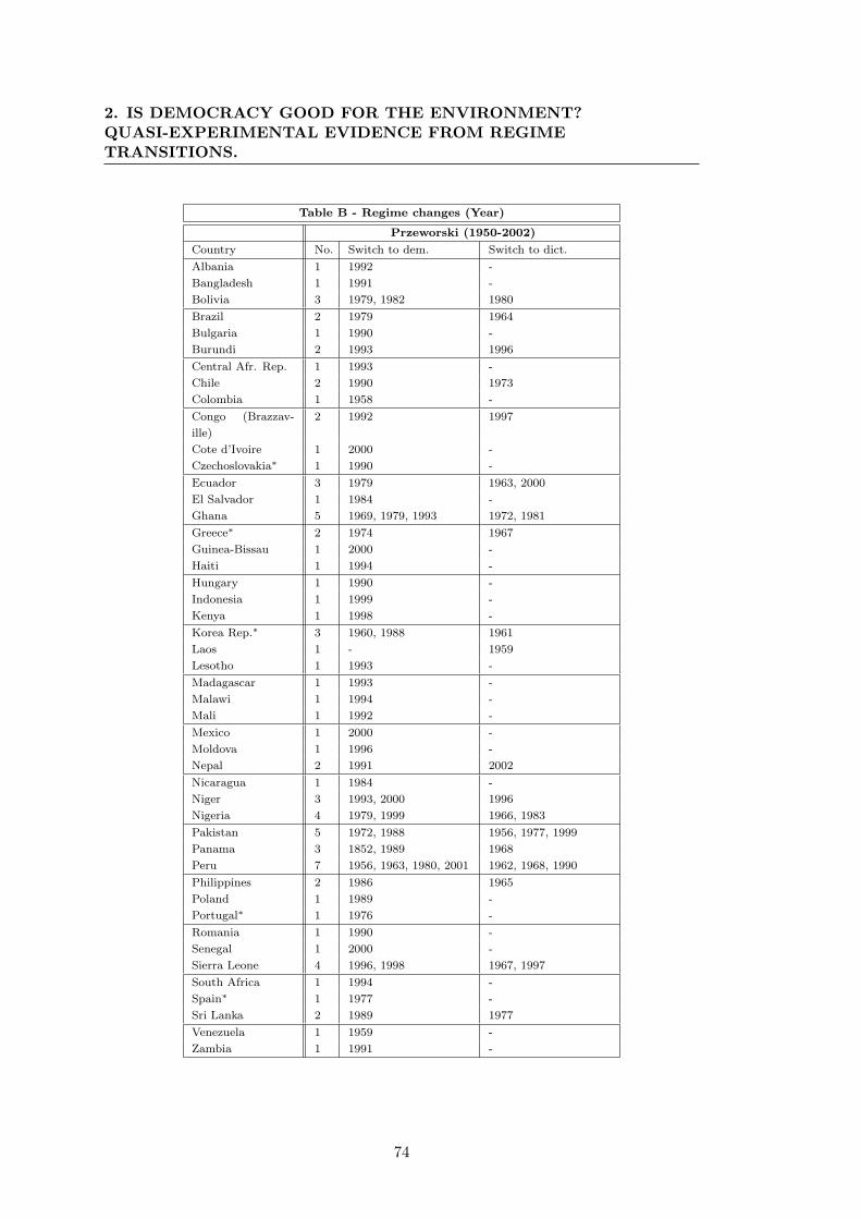
2. IS DEMOCRACY GOOD FOR THE ENVIRONMENT?QUASI-EXPERIMENTAL EVIDENCE FROM REGIMETRANSITIONS.
Table B - Regime changes (Year)
Przeworski (1950-2002)
Country No. Switch to dem. Switch to dict.
Albania 1 1992 -
Bangladesh 1 1991 -
Bolivia 3 1979, 1982 1980
Brazil 2 1979 1964
Bulgaria 1 1990 -
Burundi 2 1993 1996
Central Afr. Rep. 1 1993 -
Chile 2 1990 1973
Colombia 1 1958 -
Congo (Brazzav-
ille)
2 1992 1997
Cote d’Ivoire 1 2000 -
Czechoslovakia∗ 1 1990 -
Ecuador 3 1979 1963, 2000
El Salvador 1 1984 -
Ghana 5 1969, 1979, 1993 1972, 1981
Greece∗ 2 1974 1967
Guinea-Bissau 1 2000 -
Haiti 1 1994 -
Hungary 1 1990 -
Indonesia 1 1999 -
Kenya 1 1998 -
Korea Rep.∗ 3 1960, 1988 1961
Laos 1 - 1959
Lesotho 1 1993 -
Madagascar 1 1993 -
Malawi 1 1994 -
Mali 1 1992 -
Mexico 1 2000 -
Moldova 1 1996 -
Nepal 2 1991 2002
Nicaragua 1 1984 -
Niger 3 1993, 2000 1996
Nigeria 4 1979, 1999 1966, 1983
Pakistan 5 1972, 1988 1956, 1977, 1999
Panama 3 1852, 1989 1968
Peru 7 1956, 1963, 1980, 2001 1962, 1968, 1990
Philippines 2 1986 1965
Poland 1 1989 -
Portugal∗ 1 1976 -
Romania 1 1990 -
Senegal 1 2000 -
Sierra Leone 4 1996, 1998 1967, 1997
South Africa 1 1994 -
Spain∗ 1 1977 -
Sri Lanka 2 1989 1977
Venezuela 1 1959 -
Zambia 1 1991 -
74

2.6 Appendix
Appendix Table D - Kao residual cointegration test between CO2 and GDP
Included observations 2491
Null Hypothesis: No cointegration
Trend assumption: No deterministic trend
t-stat Prob
ADF 3.499820 0.0002
Residual variance 32630.21
HAC variance 54563.01
Augmented Dickey Fuller test equation
Dependent variable ∆εit
Method: Least squares
Included observations 2164
Variable Coeff. Std.Err. t-stat Prob
εit−1 -0.010256 0.005722 -1.792398 0.0732
∆εit−1 0.026135 0.021942 1.191083 0.2338
Appendix Table E - Johansen Fisher Panel cointegration test for CO2 and GDP
Included observations 2491
Trend assumption: No deterministic trend (restricted constant)
Lags interval (in first difference): 1 1
Unrestricted cointegration rank test (trace and maximum eigenvalue)
Hypothesized no.
of CE(s)
Fisher stat* from
trace test
Prob Fisher stat* from
max eigen. test
Prob
None 185.7 0.0000 180.7 0.0000
At most 1 83.10 0.7353 83.10 0.7353
* Prob are computed using asymptotic Chi-square distribution
Appendix Table G - Panel Unit root test summary
Exogenous variables: none
Lags included: 1
Series : Residuals from the estimation of the long run relationship
of CO2 and the other covariates (ref. table 2)
Method Stat. Prob** Cross Section Obs
Null: Common unit root process
Levin, Lin & Chu -7.72560 0.0000 40 971
Null: Individual unit root process
ADF-Fisher Chi-Square 211.779 0.0000 40 971
PP-Fisher Chi-Square 303.568 0.0000 46 1030
Series : Residuals from the estimation of the relationship
of PM10 and the other covariates (ref. table 2)
Method Stat. Prob** Cross Section Obs
Null: Common unit root process
Levin, Lin & Chu -7.96817 0.0000 25 206
Null: Individual unit root process
ADF-Fisher Chi-Square 123.941 0.0000 25 206
PP-Fisher Chi-Square 157.196 0.0000 25 206
**Probabilities for Fisher tests are computed using an asymptotic Chi-Square distribution.
All other tests assume asymptotic normality
75

2. IS DEMOCRACY GOOD FOR THE ENVIRONMENT?QUASI-EXPERIMENTAL EVIDENCE FROM REGIMETRANSITIONS.
PM10 Percapita CO2 PM10 Percapita CO2
Albania 30.81∗ -178.3 Madagascar 0 -170.3
(2.30) (-1.48) (.) (-1.46)
Bangadesh 209.1∗∗∗ -82.42 Malawi 70.41∗∗∗ -32.93
(22.13) (-0.75) (8.19) (-0.27)
Bolivia 108.9∗∗∗ -144.0 Mali 0 0
(8.72) (-1.23) (.) (.)
Brazil 15.11 -437.5∗∗∗ Mexico -4.078 -104.5
(0.82) (-3.61) (-0.19) (-0.88)
Bulgaria 49.82∗∗ 959.8∗∗∗ Moldova 34.30∗ 146.3
(2.63) (8.39) (2.59) (1.14)
Burundi 54.62∗∗∗ -60.08 Nepal 58.47∗∗∗ -85.51
(5.91) (-0.48) (6.79) (-0.71)
Central African Rep. 62.16∗∗∗ -99.27 Nicaragua 0 -344.1∗∗
(7.21) (-0.82) (.) (-3.02)
Chile 25.58 -281.6∗ Niger 0 0
(1.19) (-2.32) (.) (.)
Colombia 58.60∗∗∗ -240.6∗ Nigeria 135.9∗∗∗ 7.297
(3.54) (-1.98) (10.71) (0.06)
Congo 0 -140.5 Pakistan 204.7∗∗∗ -77.72
(.) (-1.09) (17.93) (-0.69)
Cote d’Ivoire 62.82∗∗∗ -134.1 Panama 20.78 -305.0∗
(4.13) (-1.12) (1.06) (-2.54)
Czechoslovakia -17.26 2207.3∗∗∗ Peru 53.31∗∗ -264.8∗
(-0.82) (18.50) (3.20) (-2.21)
Ecuador 18.64 -207.6 Philippines 48.12∗∗∗ -134.7
(1.13) (-1.80) (3.84) (-1.14)
El Salvador 41.90∗∗ -273.7∗ Poland 6.935 1696.4∗∗∗
(3.21) (-2.33) (0.36) (15.24)
Ghana 33.13∗∗ -101.9 Portugal 19.07 -473.3∗∗∗
(3.19) (-0.80) (0.98) (-4.09)
Greece 41.67∗ 95.11 Romania 3.696 798.1∗∗∗
(2.11) (0.79) (0.24) (5.96)
Guinea-Bissau 0 0 Senegal 84.17∗∗∗ -128.9
(.) (.) (8.09) (-1.10)
Haiti 0 -164.6 Sierra Leone 89.54∗∗∗ 20.29
(.) (-1.38) (9.31) (0.14)
Hungary -15.56 622.0∗∗∗ South Africa -9.145 1628.8∗∗∗
(-0.78) (5.92) (-0.53) (12.39)
Indonesia 83.89∗∗∗ -206.3 Spain 13.50 -185.4
(5.02) (-1.68) (0.67) (-1.55)
Kenya 47.71∗∗∗ -63.74 Sri Lanka 70.38∗∗∗ -312.3∗∗
(5.00) (-0.52) (4.78) (-2.70)
Korea Rep. 3.441 158.9 Venezuela 25.70 74.90
(0.16) (1.42) (1.40) (0.59)
Laos 0 0 Zambia 95.66∗∗∗ 83.29
(.) (.) (11.42) (0.70)
Lesotho 70.66∗∗∗ 0
(6.51) (.)
t statistics in parentheses
∗ p < 0.05, ∗∗ p < 0.01, ∗ ∗ ∗ p < 0.001
76

2.6 Appendix
The econometric model for the estimation of the unrestricted ECM for
CO2 emissions
Consider the following ARDL(1,1)
CO2it = α0i + γ1CO2it−1 +n∑j=1
δ0jXjit +n∑j=1
δ1jXjit−1 +
+4∑z=3
δ2zX4itXzit +4∑z=3
δ3zX4it−1Xzit−1 + εit (2.26)
with j = 1, ..., 4 and
X1 = GDP
X2 =√D
X3 =√A
X4 = Ineq
(2.27)
with some manipulations
CO2it − CO2it−1 + CO2it−1 = α0i + γ1CO2it−1 +n∑j=1
δ0jXjit +n∑j=1
δ1jXjit−1 +
+n∑j=1
δ0jXjit−1 −n∑j=1
δ0jXjit−1 +3∑z=2
δ2zX4itXzit +
+3∑z=2
δ3zX4it−1Xzit−1 + εit
∆CO2it = α0i − (1− γ1)CO2it−1 +n∑j=1
δ0j∆Xjit +n∑j=1
(δ0j + δ1j)Xjit−1 +
+3∑z=2
δ2zX4itXzit +3∑z=2
δ3zX4it−1Xzit−1 + εit
= α0i − (1− γ1)CO2it−1 +n∑j=1
δ0j∆Xjit +n∑j=1
(δ0j + δ1j)Xjit−1 −
−3∑z=2
δ2z∆X4it∆Xzit +4∑z=3
(δ2z + δ3z)X4it−1Xzit−1 +
+3∑z=2
δ2zX4it∆Xzit +3∑z=2
δ2z∆X4itXzit
77

2. IS DEMOCRACY GOOD FOR THE ENVIRONMENT?QUASI-EXPERIMENTAL EVIDENCE FROM REGIMETRANSITIONS.
and we end up with the usual ECM:
∆CO2it =n∑j=1
δ0j∆Xjit +3∑z=2
δ2zWz − (1− γ1)[CO2it−1 −
α0i
1− γ1−
−n∑j=1
δ0j + δ1j
1− γ1Xjit−1 −
3∑z=2
δ2z + δ3z
1− γ1X4it−1Xzit−1
]Wz =
(X4it∆Xzit + ∆X4itXzit −∆X4it∆Xzit
)
78
Bibliography
[1] Acemoglu D., Robinson J.A. and Verdier T., 2004. Kleptocracy and Divide-and-
Rule: A Model of Personal Rule. Journal of the European Economic Association,
Vol. 2, No. 2/3, Papers and Proceedings of the Eighteenth Annual Congress of the
European Economic Association, pp. 162-192. 58
[2] Barro, Robert, 1996. Getting it Right. Cambridge MA: MIT Press.
[3] Barro, Robert 1996b. Democracy and Growth. Journal of Economic Growth 1, pp.
1-27.
[4] Barro, Robert J., 1999. Determinants of Democracy Journal of Political Economy
107, pp. 158-183. 50
[5] Belk, R.W., 1988. Possession and the Extended Self, Journal of Consumer Research
5, pp. 39-47.
[3] Bhattarai M., and Hammig, M., 2001. Institutions and the Environmental Kuznets
Curve for Deforestation: a Cross Country Analysis for Latin America, Africa and
Asia. World Development 29, pp. 995-1010. 48
[7] Blanchflower, David G., and Andrew J. Oswald, 1998. What Makes a Young En-
trepreneur? Journal of Labor Economics 16, pp. 26-60.
[8] Campbell, Donald T., 1969. Reforms as experiments. American Psychologist 24,
pp. 409-429.
[9] Congleton, Roger D., 1992. Political Institutions and Pollution Control. The Re-
view of Economics and Statistics 74, pp. 412-421.
79
BIBLIOGRAPHY
[6] Dasgupta, P. and Maler, K. G., 1995. Poverty, Institutions, and the Environmental
Resource-Base, in Behrman, J., Srinivaan, T.N. (eds.), Handbook of Development
Economics, vol. 3A. Elsevier Science, Amsterdam. (Chapter 39). 48, 86
[8] Desai, Uday, 1998. Environment, Economic Growth, and Government, Ecological
Policy and Politics in Developing Countries. Albany, NY. State University Press
of New York Press, 1-45. 48, 86
[12] Engle, R.F. and C.W.J. Granger, 1987. Cointegration and Error Correction: Rep-
resentation, Estimation and Testing. Econometrica 55, pp. 251-276. 57
[13] Farzin, Y.H. and Bond, C.A., 2006, Democracy and Environmental Quality, Jour-
nal of Development Economics 81, pp. 213-235.
[14] Fisher R.A., 1932. Statistical Methods for Research Workers, 4th edition, Edim-
burgh. Oliver & Boyd. 68
[15] Frankel J.A. and Rose A.K., 2005. Is Trade Good for the Environment? Sorting
Out the Causality, The Review of Economics and Statistics 50, pp. 85-91.
[12] Gallagher K. P., and Thacker S. C., 2008. Democracy, Income and Environmental
Quality, Political Economy Research Institute (PERI) Working Paper No. 164,
University of Massachusetts Amhrest. 49
[17] Gaspart F., and Platteau, J.P., 2007. Heterogeneity and Collective Action for Ef-
fort Regulation: Lessons from the Senegalese Small-Scale Fisheries, in Inequality,
Cooperation and Environmental Sustainability, edited by Baland J.M., Bardhan
P., and S. Bowles, Princeton University Press.
[13] Gleditsch, Nils P., and Bjorn Sverdrup, 2003. Democracy and the Environment.
In Human Security and the Environment: International Comparisons, edited by
Edward Paper and Michael Redclift. London: Elgar. 48, 86
[15] Grossman, G.M., and Krueger, A.B., 1995, Economic Growth and the Environ-
ment, Quarterly Journal of Economics 110, pp. 353-377. 102
[16] Hardin, Garret, 1968. The Tragedy of the Commons. Science 162, pp. 1243-1248.
48, 86
80

BIBLIOGRAPHY
[21] Hausman, Jerry, 1979. Individual Discount Rates and the Purchase and Utilization
of Energy-using Durables, Bell Journal of Economics 10, pp. 33-54. 50
[22] Heerink N., Mulatu A., and Bulte E., 2001. Income Inequality and the Environ-
ment: Aggregation Bias in Environmental Kuznets Curves. Ecological Economics
38, pp. 359-367.
[23] Holtz-Eakin Douglas, David Joulfaian and Harvey S. Rosen, 1994. Sticking it Out:
Entrepreneurial Survival and Liquidity Constraints. Journal of Political Economy
102, pp. 53-75.
[24] Hwang Hsiang-Chih, 2006. Water Quality and the End of Communism: does a
Regime Change Lead to a Cleaner Environment?. Brandeis University Working
Paper.
[25] Im, K.S., M.H. Pesaran and Y. Shin, 2003. Testing for Unit Roots in Heterogeneous
Panels. Journal of Econometrics 115, pp. 53-74. 66
[26] International Monetary Fund, 2009. World Economic Outlook Report.
[27] Kao Chihwa, 1999. Spurious Regression and Residual-Based Tests for Cointegra-
tion in Panel Data, Journal of Econometrics 90, pp. 1-44. 55, 68
[20] Leslie, Winsome J., 1987. The World Bank and Structural Transformationin De-
veloping Countries:The Case of Zaire. Boulder, CO: Lynne Rienner Publishers.
58, 86
[29] Levin A., C.F. Lin and C. Chu, 2002. Unit Root Test in Panel Data: Asymptotic
and Finite-Sample Properties. Journal of Econometrics 108, pp. 1-24. 65
[30] Levine, James, 1997. Badass Sells, Forbes 159, pp. 142-147.
[31] Li Q. and Reuveny R., 2006. Democracy and Environmental Degradation. Inter-
national Studies Quarterly 50, pp. 935-956.
[32] Maddala G.S. and Shaowen Wu, 1999. A Comparative Study of Unit root test with
Panel Data and a New Simple Test, Oxford Bulletin of Economics and Statistics
61, 631-652. 55, 68
81
BIBLIOGRAPHY
[21] Maddison Angus, 2009. Statistics on World Population, GDP and
Per Capita GDP, 1-2006 AD, updated March 2009, available at
http://www.ggdc.net/maddison/ 52, 96
[22] Marland, G., T.A. Boden, and R. J. Andres, 2008. Global, Regional, and National
CO2 Emissions. In “Trends: A Compendium of Data on Global Change”. Car-
bon Dioxide Information Analysis Center, Oak Ridge National Laboratory, U.S.
Department of Energy, Oak Ridge, Tenn. 52, 96
[35] Marland G., and R.M. Rotty, 1984. Carbon Dioxide Emissions from Fossil Fuels:
a Procedure for Estimation and Results for 1950-82. Tellus 36(B), pp. 232-261. 52
[36] Mason R., 1981. Conspicuous Consumption: A Study of Exceptional Consumer
Behaviour, St. Martin’s Press, New York, NY.
[37] Midlarsky Manus, 1995, Environmental Influences on Democracy: Aridity, War-
fare and a Reversal of the Causal Arrow, The Journal of Conflict Resolution 39,
pp. 224-262.
[38] Midlarsky Manus, 1998, Democracy and the Environment: An Empirical Assess-
ment, Journal of Peace Research 35, pp. 341-361.
[39] Milanovic Branko, 2000. The Median Voter Hypothesis, Income Inequality and
Income Redistribution: an Empirical Test with the required data, European Journal
of Political Economy, September 2000. 48
[25] Moya Pons, Frank, 1995. The Dominican Republic: A National History. Princeton,
NJ: MarkusWeiner. 58, 86
[26] Olson, Mancur. 1965. The Logic of Collective Action. Harvard University Press.
[28] Payne Rodger A., 1995, Freedom and the Environment, Journal of Democracy 6,
pp. 41-55.
[43] Przeworski A. and Limongi F., 1993. Political Regimes and Economic Growth, The
Journal of Economic Perspectives 7, pp. 51-69. 48, 86
[44] Rodrik Dani, 1999. Democracies Pay Higher Wages, Quarterly Journal of Eco-
nomics 114, pp. 707-738. 50
82

BIBLIOGRAPHY
[30] Schultz, C. B., and T. R. Crockett, 1990 Economic Development, Democratization,
and Environmental Protection in Eastern Europe. Boston College Environmental
Affairs Law Review 18, pp.5384. 48
[34] Torras M., and Boyce J. K., 1998. Income, Inequality and Pollution: a Reassess-
ment of the Environmental Kuznets Curve. Ecological Economics 25, pp. 147-160.
48, 86
[47] United Nations, 1992. Handbook of the International Comparison Program. 48
[48] Urbain, J.P., 1992. On Weak Exogeneity in Error Correction Models. Oxford Bul-
letin of Economics and Statistics 54, pp. 187-207. 72
[49] Veblen T., 1934. The Theory of the Leisure Class, Random House, Inc., New York,
NY. 55, 70
[50] Waller M., and Millard, F., 1992. Environmental Politics in Eastern Europe. En-
vironmental Politics 1, pp. 159-185.
[51] Wittfogel Karl, 1957. Oriental Despotism: a Comparative Studies of Total Power,
New Haven CT: Yale University Press.
83

BIBLIOGRAPHY
84

3
Democratisation, Environmental
and Income Inequality.
Abstract
Empirical economists commonly agree upon the fact that the demand for environmentalgoods is increasing with income, so as long as democratisation shifts the decisive power froma rich individual (autocrat or dictator) to a poorer one (decisive voter), such a regime changeshould be associated to worse environmental conditions. Assuming that citizens’ wealth doesnot depend on inherited endowments, but only on each individual’s share on total production, Iwill show with a theoretical model that contrary to the expectations, democratisation may havemixed effects on the level of environmental quality, depending on the size of the price and incomeeffects on the demand for environmental quality associated to a decrease in the decisive politicalactor’s wealth. If indeed a poorer individual desires less environmental quality than a richerindividual (income effect), he also desires less of the goods responsible for degradation (priceeffect) so the overall result on the environment is ambiguous. Assuming instead that societyis composed by two classes of individuals, one supplying an embodied factor of productionand one supplying capital, and assuming moreover that the decisive voter belongs to the firstclass of individuals while the autocrat does not, democratisation is shown to be beneficial forthe environment, the better the effect on the environment, the bigger the difference in wealthbetween the two decisive political actors.
JEL Classification: D02, D31, O13, Q56
Keywords: Democracy; Environment; Environmental Inequality; Income Inequality.
85

3. DEMOCRATISATION, ENVIRONMENTAL AND INCOMEINEQUALITY.
3.1 Introduction
Theoretical and empirical literature about the effects of democracy on the level of environmentalquality is still inconclusive and does not provide clear and unilateral answers to the effectof different regimes on the environment. In the seventies, the dominant thinking was thatdemocracy and its associated liberties to consume and procreate would have generated ecologicalcatastrophes (Desai, (8), Hardin, (16)); recently, on the contrary, scholars have found positiveeffect of democracy on the environmental quality, the main reason being the necessity fordemocratic governments to be elected or re-elected, which makes them more prone to respecthuman life, and then more responsive to life threatening environmental degradation (Dasguptaand Maler (6), Schultz and Crockett (30), Payne (28), Gleditsh and Sverdrup (13)).
This paper is aimed at contributing on the debate about whether democracy may be goodor not for the environment. The questions I want to answer are: what is the role of a polit-ical regime in the determination of a country’s environmental policy? Are democracies moreenvironmentalist than autocracies? In order to answer these questions, it is important first ofall to understand the difference between those two regimes. In a (direct) democracy, decisionsare taken by majority voting, while in a dictatorship they are taken by one or a group of fewindividuals. In practice, therefore, the decisive political actor is different, and what makes themdiffer is often their wealth.
It is well known that wherever in the world, at any time in history, kings, queens anddictators have been the richest and powerful people. From north to south, in developed andunderdeveloped countries, in communist and non-communist countries, the only characteristicthat this variegated group of people has in common is a lofty position and vast fortune. Forbes,in an article appeared few years ago1, estimated the Saudi Arabia King Abdullah Bin Abdu-laziz’s wealth in around 45% of the country’s $340 billion GDP. Brunei’s Sultan Haji HassanalBdkiah has an estimated fortune of $20 billion, and benefits from petroleum and natural gasfields. The President of the United Arab Emirates, Sheikh Khalifa bin Zayed Al Nahyan ownthe 90% of the 2.5 million barrels a day exported from the UAE and he alone represents twothird of the GDP. Mutubu Sese Seko in the Democratic Republic of Congo (Zaire) during the70’s benefitted of around 15-20% of Congo’s operating budget and in the 80’s his fortune wasestimated in $5 billion (Leslie (20), p. 72). Rafael Trujillo in the Dominican Republic had afortune which amounted to 100% of the national GDP at current prices and his family con-trolled almost 80% fo the country’s industrial production (Moya Pons (25), p. 398). Theseare only few examples, but the list of very rich rulers is not over and probably it would be amanuscript on its own. From this perspective, a regime change from dictatorship to democracyshifts the decision power from the dictator to the median voter, implying an impoverishmentof the decisive political actor and therefore a different willingness to pay for environmentalprotection.
1The article is available online at http://www.forbes.com/2006/05/04/rich-kings-
dictators cz lk 0504royals.html
86

3.1 Introduction
If the demand for environmental quality was an increasing function of income, dictatorshipwould be a panacea for the environment. Numerous empirical studies suggest that willingness topay for environmental improvement is an increasing function of wealth (Hokby and Soderqvist(17), Kristrom and Riera (18), Miles, Pereyra and Rossi (24)). Richer people tend to expresshigher willingness to pay for environmental improvement than poorer people, that is, environ-mental quality is typically found to be a normal good. Because of this, an institutional shiftfrom democracy to dictatorship should result in an improvement of a country’s environmentalquality. As pointed out by Boyce, (4), however, this beneficial effect may not necessarily bringto the expected result, because other factors come into play to mitigate or even nullify it.
First, because an increase in the decisive political actor’s income raises his “price” of theenvironmental protection. Increasing income means increasing the share the individual gets outof production, if production is kept constant. Since production requires some environmentaldepletion, it is easy to realise that environmental protection is more costly for the rich because adecrease in global GDP results in a greater decrease in his own income than on the poor’s, whogets a lower share. Moreover, even though richer individuals may desire more environmentalquality (income effect), they also desire more of the goods and services responsible for environ-mental degradation (price effect), so the expected environmental improvement will occur onlyif the negative “price effect” does not outweigh the positive “income effect”.
Second, because richer people have more resources and capabilities to substitute environ-mental quality with private consumption, giving raise to the so-called environmental inequality.If indeed the willingness to pay (WTP) for environmental protection is an increasing functionof income, different is the elasticity of such willingness to pay. Martini and Tiezzi (23) indeedfind, in a panel of Italian households from 1999 to 2006, that despite the willingness to payfor environmental protection is higher for richer people, the elasticity of WTP is less than one,and therefore decreases as income increases, suggesting a lower capability for poorer people tosubstitute environment with private consumption.
Substantial evidence shows indeed that the less wealthy and powerful members of societiesmay be the ones exposed to much heavier environmental degradation than the more well off,being able to avoid it, simply relocating to cleaner living areas or using their political powerto drive out polluting industries from their neighborhoods. Gray and Shadbegian (14), forinstance, obtain some evidence from US data on the paper industry for the period 1985-1997that polluting emissions are significantly lower in areas with more children, older people andfewer poor people than in areas with young poor people without children, and Bina Agarwal (2),for instance, documented how the degradation of forest resources in rural India had particularlysevere effects on poor women, via impacts of their time, income and nutrition. Pastor, Saddand Hipp (27), for instance, provide substantial evidence that minorities residential areas havean higher likelihood to host various environmental hazards, and Sheila Foster (11) reports thatpoor african american neighbourhoods in Chester (Pennsylvania) often experience a clusteringof waste facilities in their areas.
In this paper, I provide a theoretical model through which I analyse the effects of democrati-
87

3. DEMOCRATISATION, ENVIRONMENTAL AND INCOMEINEQUALITY.
sation on the environment, meaning by democratisation a shift of the decisive power from arich individual (dictator) to a poorer one (decisive voter). I will assume that citizens differonly by their wealth, meaning by wealth only income (or share they get out of production) andexcluding any inherited endowment, to keep the model as simple as possible.
In the first instance, I will analyse the result of democratisation on the level of environmentalquality assuming that there is no environmental inequality, so all the citizens experience thesame level of pollution.
I will later remove this assumption by introducing a class model of experienced pollution,and assuming that the society is composed by two types of individuals - employers and employ-ees. Employers supply capital in the production process, while employee supply their physicallabor and therefore cannot avoid their own exposure to pollution. Employers, on the otherhands, supplying capital, can relocate far away (at a cost) from their polluting factories, beingnot necessary their physical activity in the production process.
As it is often unexpected, income inequality per se between the two decisive political actorsmay not be responsible of different environmental policies undertaken by the two differentregimes, but environmental inequality is the crucial variable affecting them. Income inequality,therefore, has an indirect role as long as it induces environmental inequality. In countries wherethe majority of the population is represented by employees whose services require physicalpresence in the firm, democratisation is expected to be beneficial for the environment, and thisis in line with the recent empirical evidence.
The next section introduces the model. Section 3.3 presents some empirical evidence anddiscusses some cases of regime transition, having regards to the effect on environmental policyof democratisation. Section 3.4 concludes.
3.2 The model
This section presents the model, with the aim of analysing the effect of a regime change (inparticular, democratisation) on the optimal level of environmental quality. In the first instance,I will assume that the decisive political actor in autocracy is richer than in democracy, sodemocratisation results in a shift of the decisive power from a rich individual (the dictator) toa poor one (the median voter). Poorer people have a tendency to value consumption more thanenvironmental quality, but richer people consume more of the good which are responsible forpollution. The first part of the model will deal with this issue, assuming that the environmentis a pure public good whose exposure cannot avoided by anyone at any cost.
The second part instead will introduce a model of class differences in experienced envi-ronmental quality to take into account of the effect of environmental inequality. Assumingthat the decisive political actors in democracy and autocracy belong to different classes, andin particular, assuming that the dictator is a capitalist employer who supply only capital inthe production process and therefore is able to relocate his home far away from the pollut-ing sources, while the median voter is a employee who supply physical labor and therefore is
88

3.2 The model
exposed to emission, I will show that democracy is beneficial to the environment, the morebeneficial the higher the difference in wealth between the dictator and the median voter.
3.2.1 Democratisation and income inequality
Throughout this section, I will assume that:
A. 1 The decisive political actor under an autocratic regime receives a larger share of GDPthan under a democratic one.
Denote then by g the level of production, or GDP, and by e the level of environmental quality,with both g and e assured to be positive. Environment is an essential factor of production,so there cannot be positive production without some environmental depletion. Equation 3.1represents the relation between production and environmental quality, i.e., the transformationlocus between environment and income:
g = f − 12e2 (3.1)
with f a positive constant. The maximum achievable level of production is bounded above dueto technological constraints and this boundary is represented by f . A level of production equalto f can be achieved only by completely depleting the environment. Conversely, the highestenvironmental quality requires absence of production.
Suppose than that the society is composed by N individuals, with all having identical pref-erence function. Each generic individual i gets a share of total production si, with
∑Ni=1 s
i = 1(notice that, in general, in general si 6= sj for i 6= j) as a “personal wage” available for con-sumption, and therefore, the amount each individual can consume in each period is representedby
yi = sig (3.2)
and therefore, the “personal” marginal rate of transformation between income and environmen-tal quality is represented by
∂yi
∂e= −esi. (3.3)
Each individual’s utility is a nonseparable function of income and environmental qualityand it is denoted by
ui = u(yi, e) i = 1, ..., N (3.4)
with ui representing the level of utility for individual i, yi denotes income (or consumption) ofthe same individual, and e the level of environmental quality. Environmental quality is a publicgood which is experienced uniformly across the population, hence the absence of the superscript(this assumption, however, will be removed later). The utility function ui is assumed increasingand concave with respect to both arguments, and have positive cross derivates. In other words,I have ue > 0, uy > 0, uee < 0, uyy < 0, uey > 0 and uye > 0, where ux is the first derivativeof the utility function with respect to the generic variable x and uxz is the first derivative of
89

3. DEMOCRATISATION, ENVIRONMENTAL AND INCOMEINEQUALITY.
ux with respect to another variable z. These assumptions imply that the utility generated byincreasing income or environmental quality is positive, but it increases at a decreasing rate,and that the pleasure derived by income (cleaner environment) is higher, the higher is theenvironmental quality (income).
Under assumption A.1., if the level of experienced environmental quality does not differbetween different people, the effect of democratisation (autocratisation) can be read as theeffect of an impoverishment (enrichment) of the decisive political actor. Denote with v thedecisive political actor under democracy, and with a the decisive individual under autocracy.Assumption A.1. has the only implication that sv < sa, so the problem the decisive citizenfaces is
maxeui = u(yi, e) i = v, a (3.5)
s.t. yi = si · g (3.6)
g = f − 12e2 (3.7)
so they decide their optimal levels of environmental quality so as to maximise their utilitysubject to their wealth and the available technology.The first order condition for utility maximisation requires
− sie · uyi(yi, e) = −ue(yi, e) or (3.8)
−esi = − ue(yi, e)uyi(yi, e)
(3.9)
where uyi represents the derivative of the utility function for individual i with respect to the levelof income yi, and ue represents the derivative of the utility for individual i with respect to theenvironmental quality. Equation 3.9 simply says that as a necessary condition for maximisingutility is the equality between the “personal” marginal rate of transformation between incomeand environment and the marginal rate of substitution between income and environment. Thelevel of environmental quality e chosen by individual i, therefore, will be
e∗ =1si· ue(yi, e)uyi(yi, e)
. (3.10)
A first question that comes into mind is whether the effect of a marginal increase in theshare of income of this citizen increases the level of environmental quality or not. Taking thefirst derivative of e∗ with respect to si, we get that
∂e∗
∂si=
1si
[− 1si
(ue(yi, e)uyi(yi, e)
)+
+ g
(ueyi(yi, e)uyi(yi, e)− ue(yi, e)uyiyi(yi, e)
(uyi(yi, e))2
)](3.11)
which is positive (so the effect of an increase in si is good for the environment) when
90

3.2 The model
1sig
< −uyiyi(yi, e)uyi(yi, e)
+ueyi(yi, e)ue(yi, e)
. (3.12)
Defining
ue(yi, e)uyi(yi, e)
= MRSie,y (3.13)
−esi = MRT ie,y (3.14)
it is easy to see that equation 3.12 can be rewritten as1
∂MRT ie,y/∂y
MRT ie,y/y
<∂MRSi
e,y/∂y
MRSie,y/y
(3.15)
so, a positive variation in the share of income is associated to a positive variation in the levelof environmental quality only if the “price effect” due to an higher share of income si (whichmakes also the marginal rate of transformation between environment and income steeper) islower than the “income effect” due to the relative variation in the marginal rate of substitutionbetween the two goods. In other words, becoming richer is beneficial for the environment onlyif the elasticity of MRT i
e,y is lower than the elasticity of MRSie,y, both with respect to income.
Denoting by ev and ea the optimal level of environmental quality chosen, respectively, bythe decisive citizen in democracy and by the dictator, we have that
ev =uev (yv, ev)
sv · uyv (yv, ev)(3.16)
ea =uea(ya, ea)
sa · uya(ya, ea)(3.17)
The optimal level of environmental quality selected in democracy will be lower than thelevel selected in dictatorship (ev < ea) if
MRSve,y
svg<MRSa
e,y
sag(3.18)
or, rearranging,MRSv
e,y
sv<MRSa
e,y −MRSve,y
sa − sv(3.19)
Equation 3.18 highlights the ambiguous effect (depicted in figure 1) of a regime shift. Sincethe level of environmental quality experienced by both the dictator and the decisive citizen indemocracy is actually the same, what makes the difference in determining which regime is morepro-environment depends basically on the difference between “relative” marginal willingness topay for environmental protection. An example may clarify the interpretation of equation 3.18.Suppose the decisive political actor in democracy is willing to pay 2 unit of income to increase
1For the computation of the derivative with respect to y of the marginal rate of transformation,
we make use of equation 3.6 according to which si = yi/g. Substituting si into 3.14 and taking the
derivative with respect to yi, we get −e/g, which, once divided by −esi gives 1/sig.
91

3. DEMOCRATISATION, ENVIRONMENTAL AND INCOMEINEQUALITY.
by one unit environmental quality. Suppose instead that the dictator is willing to pay 5, becausehe’s richer so he values environment more. However, the difference in wealth between thosetwo decisive citizens is huge. Suppose that the dictator gets 10% of the global production, sosa = 0.1. Assume that the median voter gets only 1%, so sv = 0.01. Assume that the country’sGDP (g) is, for simplicity, 1000. It follows that, in percentage, the decisive political actor indemocracy is willing to give up 0.2% of his income to protect the environment while the samedecisive citizen under dictatorship is willing to pay 5%. In this case, of course, democracy isbad for the environment. If inequality between those two citizens instead was not too high,and the marginal rate of substitution for the median voter was 6 against 8 for the dictator,sv = 0.05, sa = 0.1, and keeping constant g at 1000, we have that proportionally to income,the median voter is willing to give up 12% of to increase environmental quality against 8% forthe dictator. This case, of course, implies that democracy is good for the environment.
Figure 1 provides a graphical explanation of the argument above. Suppose that the decisivecitizen’s income increase from svg to sag. Whether this shift is good for the environment or not,depends on the variation of the ratio between the two marginal rates of substitution betweeny and e for the dictator and the decisive citizen in democracy. Of course, the dictator has aMRSe,y higher than the median voter’s MRSe,y, but if this increase in the willingness to payfor environmental quality do not compensate the increase in the share of income the dictatorgets, dictatorship is bad for the environment (figure 1A). Figure 1B depicts the opposite case,so when democracy is bad for the environment, because the marginal utility from consumptionof the decisive voter in democracy is much higher than the dictator’s one, so a shift fromdemocracy to dictatorship is good for the environment. Equation 3.18 mans exactly what isdepicted in figure 1.
Figure 1.
From another point of view, equation 3.19 shows that we can see democratisation as a badregime for the environment if the median voter’s relative marginal willingness to pay for envi-ronmental quality does not compensate what would be the difference of the marginal willingnessto pay under the two different regimes, weighted by the difference in income between the twodecisive citizens.
92

3.2 The model
3.2.2 A model of class differences in experienced environmental qual-
ity
In order to introduce environmental inequality, i.e., the fact that environment is experiencedin different ways by different people, I will make the assumption that the population is dividedinto two classes, capitalists and workers. Capitalists supply capital in the production processand receive the rents their capital generates. Workers can only sell their labour in the firmsowned by the capitalists and therefore cannot avoid their exposure to the pollution producedby the firms they are employed in, either because during the job they are exposed to emissions,or because they cannot relocate too far away from the firms since they have to show up atwork every morning. Of course, this is not the case for the capitalist, who can choose thebest location to live because he does not need to physically sell his own labour. Under theassumption that the decisive political actor in autocracy is a capitalist and in democracy is aworker, the optimal level of environmental quality chosen by those two decisive citizens will bedifferent than in the previous case. The worker is assumed to have an experienced environmentalquality which reflects the real status of the environment, therefore his maximisation problemremains unchanged. The capitalist, on the contrary, may decide to increase his own perception1
of environmental quality, for example, by relocating in a cleaner area, but this can be done ata cost. The price may be related, for instance, to the transportation costs the capitalist mustpay in order to reach the city where his firms are located, so the price may be a function of thecapitalist’s home distance to the industrial district.
Denote by eax the capitalist’s (or dictator) level of experience environmental quality. ea
x isno more equal to the actual, or “real” level, since it can be increased by relocating far awayfrom the pollution source. In detail, the equation for ea
x is given by
eax = e+ hc (3.20)
where e is the real level of environmental quality, c is the cost of relocating in a cleaner areaand h is a positive constant denoting the level of “productivity” of the cost of living far fromthe pollution sources. In this model, we will assume that
eax ≥ e (3.21)
so the level of experienced environmental quality cannot be lower than the real level. Thisassumption guarantees that c is an effective cost, so it cannot be negative (the employer basicallycannot accept bribes in order to live close to the polluting factory).
Equation 3.20 can be rephrased as follow: if one defines c the monetary expense the employerpays to experience a better environment, c can be read as
c = p(eax − e) (3.22)
1“Perceived” environmental quality may differ to “experienced” environmental quality in the sense
that the perception of the environment may be subjective and mistaken. In this paper however, I
consider the words “perceived” and “experienced” as a synonymous because I exclude the possibility
that a person may perceive pollution differently from other people in the same class or even wrongly.
93

3. DEMOCRATISATION, ENVIRONMENTAL AND INCOMEINEQUALITY.
that is to say, the price for an experienced environmental improvement (p) multiplied by thedifference in the experienced environmental quality chosen by the employer and the real en-vironmental quality (ea
x − e). If this is the case, it is possible to notice, by equation 3.20,that, taking e from the right hand side of the equation to the left, the price for an experiencedenvironmental improvement p is defined as 1/h.
p ≡ 1h
(3.23)
Since the capitalist - or employer - pays a cost c > 0, his level of income available forconsumption will be reduced of that amount, so
ya = sag − c (3.24)
and technology remains identified by equation 3.1.The new problem the decisive political actor in dictatorship faces is then
maxe,c
ua = u(ya, eax) (3.25)
subject to equation 3.20 and 3.24. The first order conditions for utility maximisation are:
∂ua
∂e= 0 ⇒ ea∗ =
ueax(ya, ea
x)sauya(ya, ea
x)(3.26)
∂ua
∂c= 0 ⇒ 1
h=ueax
(ya, eax)
uya(ya, eax)
(3.27)
Equation 3.27 represents the equilibrium level of expenditure, which must equate the pro-ductivity of the “insurance” against pollution and the amount of the environmental quality thedictator is willing to give up to become one unit richer. Combining equations 3.26 and 3.27 Iget
ea∗ =1sah
(3.28)
so the optimal level of environmental quality chosen by the dictator depends negatively onlyon the share he can get out of production and the productivity of the expenditure in increasingthe perception of environmental quality.
The reason for this result is simple: a richer citizen enjoys environmental quality more thana poor one, but his opportunity cost to pay for environmental protection is higher than for apoor citizen. If he can increase his own perception of environmental quality of an amount thatis greater than the amount of environment he is willing to give up to become one unit richer,then it is worthwhile to pay.
In general, taking the equilibrium relations of the two decisive political actors, representedby equation 3.28 and equation 3.16, I get that the optimal level of environmental quality willbe lower in autocracy if
h >sv
sa· uyv (yv, ev)uev (yv, ev)
(3.29)
that is to say, if the level of productivity of the cost devoted to prevent exposure to pollutionis greater than the amount of environmental quality the median voter is willing to give up
94

3.2 The model
to become a unit richer, times the ratio of the income share of production of the two decisiveactors. So, income inequality between the dictator and the median voter is not a good predictorof the effect of a regime change on the environmental policy undertaken by a country, it isenvironmental inequality that matters, as long as the expenditure for substituting environmentwith private consumption is productive (i.e. increase the perception of environmental quality)enough. This result is exacerbated when income inequality between the two political actors isbig, making autocracy more prone to choose bad environmental policies even for lower levels ofh.
Figure 2 represents two possible equilibria that a country may end-up in, depending on thetype of regime. Assume that a dictator gets a larger share of output than a potential medianvoter in a democracy; if the dictator can pay to avoid his own exposure to pollution and themedian voter cannot, the dictator will choose a lower optimal level of environmental quality.Denote by svy − emax and say − emax the private transformation locus between income ofthe potential median voter and the dictator, respectively. At point c the median voter solveshis own maximisation problem, equating his MRSe,y (that is to say, the amount of money heis willing to spend to improve the environment) with the amount of money he would get byproducing more (this is expressed in terms of e, and is equal to −se). Denote this equilibriumlevel of environmental quality by e∗v. The dictator optimises his utility function with respectto two controls, the level of perceived environmental quality and the cost of insurance againstexposure to pollution. The equilibrium condition is represented by equation 3.28.
Figure 2
The question is: if the dictator can protect himself against pollution by paying an insurance,will his optimal level of e be lower than the optimal level of the median voter? The answeris yes, provided that at point d the amount of income the dictator has to give up to increase
95
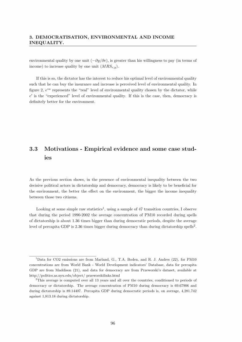
3. DEMOCRATISATION, ENVIRONMENTAL AND INCOMEINEQUALITY.
environmental quality by one unit (−∂y/∂e), is greater than his willingness to pay (in terms ofincome) to increase quality by one unit (MRSe,y).
If this is so, the dictator has the interest to reduce his optimal level of environmental qualitysuch that he can buy the insurance and increase is perceived level of environmental quality. Infigure 2, e∗a represents the “real” level of environmental quality chosen by the dictator, whilee′ is the “experienced” level of environmental quality. If this is the case, then, democracy isdefinitely better for the environment.
3.3 Motivations - Empirical evidence and some case stud-
ies
As the previous section shows, in the presence of environmental inequality between the twodecisive political actors in dictatorship and democracy, democracy is likely to be beneficial forthe environment, the better the effect on the environment, the bigger the income inequalitybetween those two citizens.
Looking at some simple raw statistics1, using a sample of 47 transition countries, I observethat during the period 1990-2002 the average concentration of PM10 recorded during spellsof dictatorship is about 1.36 times bigger than during democratic periods, despite the averagelevel of percapita GDP is 2.36 times bigger during democracy than during dictatorship spells2.
1Data for CO2 emissions are from Marland, G., T.A. Boden, and R. J. Andres (22), for PM10
concentrations are from World Bank - World Development indicators’ Database, data for percapita
GDP are from Maddison (21), and data for democracy are from Przeworski’s dataset, available at
http://politics.as.nyu.edu/object/ przeworskilinks.html2This average is computed over all 13 years and all over the countries, conditioned to periods of
democracy or dictatorship. The average concentration of PM10 during democracy is 69.67906 and
during dictatorship is 89.14407. Percapita GDP during democratic periods is, on average, 4,281.742
against 1,813.18 during dictatorship.
96
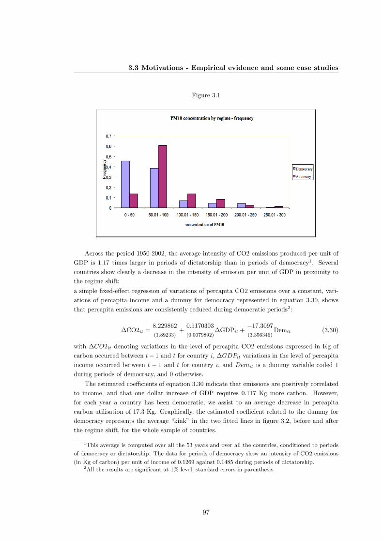
3.3 Motivations - Empirical evidence and some case studies
Figure 3.1
Across the period 1950-2002, the average intensity of CO2 emissions produced per unit ofGDP is 1.17 times larger in periods of dictatorship than in periods of democracy1. Severalcountries show clearly a decrease in the intensity of emission per unit of GDP in proximity tothe regime shift:
a simple fixed-effect regression of variations of percapita CO2 emissions over a constant, vari-ations of percapita income and a dummy for democracy represented in equation 3.30, showsthat percapita emissions are consistently reduced during democratic periods2:
∆CO2it =8.229862(1.89233)
+0.1170303(0.0079892)
∆GDPit +−17.3097(3.356346)
Demit (3.30)
with ∆CO2it denoting variations in the level of percapita CO2 emissions expressed in Kg ofcarbon occurred between t− 1 and t for country i, ∆GDPit variations in the level of percapitaincome occurred between t − 1 and t for country i, and Demit is a dummy variable coded 1during periods of democracy, and 0 otherwise.
The estimated coefficients of equation 3.30 indicate that emissions are positively correlatedto income, and that one dollar increase of GDP requires 0.117 Kg more carbon. However,for each year a country has been democratic, we assist to an average decrease in percapitacarbon utilisation of 17.3 Kg. Graphically, the estimated coefficient related to the dummy fordemocracy represents the average “kink” in the two fitted lines in figure 3.2, before and afterthe regime shift, for the whole sample of countries.
1This average is computed over all the 53 years and over all the countries, conditioned to periods
of democracy or dictatorship. The data for periods of democracy show an intensity of CO2 emissions
(in Kg of carbon) per unit of income of 0.1269 against 0.1485 during periods of dictatorship.2All the results are significant at 1% level, standard errors in parenthesis
97

3. DEMOCRATISATION, ENVIRONMENTAL AND INCOMEINEQUALITY.
Figure 2.1 shows, for Colombia, South Africa, Spain and Bulgaria, the actual (dotted) andfitted (line) levels of intensity of emissions (expressed in tons of carbon per unit of GDP). Thevertical line in each subfigure represents the date of the regime shift. All the four countrieshave experienced a transition to democracy after long periods of dictatorship. After the regimeshift we observe a reverse pattern for emissions; while before democratisation the tendency isto increase the intensity of CO2 emissions in production, later we observe a decline, which ispersistent through time.
98

3.3 Motivations - Empirical evidence and some case studies
Figure 3.2
In early democracies, environmental policies may be often out of the public agenda. Theneeds of protecting human rights are instead one of the main reason for democratisation. Theprotection of human rights often manifests as the need of a job for everyone, social reformsaimed at reducing poverty and pressures for meeting the basic needs for the whole population.In this last category falls the right of everyone to have an healthy life for the present and futuregenerations, and therefore environmental management becomes of crucial importance. How acountry chooses to achieve the goal of a better environment however varies between differentnations, and sometimes it is a direct consequence of other policies undertaken and may not beexplicitly regulated. In Colombia, for example, the sharp reduction in the intensity of emissionis associated with the land reform which was aimed both at creating jobs and reducing poverty.Under the President Carlos Lleras Restrepo (1966-1970) the Colombian Instutute of AgrarianReform (INCORA) promoted the redistribution of usable land to the peasants and unemployedworkers in the country, issuing more than 60.000 titles in 1968 and 1969 alone. As a resultof that, after few years the economy was more diversified than before, labor productivity washigher, and inequality lower. He also implemented an aggressive and broad program of socialand economic reforms, creating, among others, a national saving fund, an institute for thefamily wellbeing, the institute to protect non-renewable resources, an agency to promote exportetc. His successor Misael Pastrana Borrero (1970-1974) carried on the development increasingeconomic growth through encouraging housing construction and giving financial incentives tocommercial agriculture. As a result jobs increased as well as wages, and he also promoted thefirst national environmental legislation in Latin America.
99

3. DEMOCRATISATION, ENVIRONMENTAL AND INCOMEINEQUALITY.
In South Africa the picture is similar. The election of the new government in 1994 wasmeant to put in place new policies to promote development, directed mainly at alleviatingpoverty, creating jobs and meeting the basic needs for the majority of South Africans. In thislast context, it was necessary to define a clear policy objectives in the area of environmentalquality and the use of natural resources. The Constitution provided (and provides) a powerfulsafeguard in shaping future economic and social development in an environmentally sustainableway: it lays down among the fundamental rights of every citizen that “every person shall havethe right to an environment that is not detrimental to his or her health and wellbeing” andthat “every person shall have the right to access to all information held by the state or any ofits organs at any level of government insofar as such information is required for the protectionor exercise of any of his or her rights”.
In Spain the decrease in the intensity of emission coincides with an increase in the invest-ments in environmental areas. During the sixties and the early seventies Spain have had anuncontrolled process of industrialisation (Font and Morata (10)). The institutionalisation of theenvironmental policy started in the seventies, with the creation in 1971 of the InterministerialCommission for the Environment, but investments in the environmental areas were not signifi-cant until 1978 (De Esteban and Lopez Lopez (7)), when the new Constitution introduced anarticle that ascribes as duty to ensure rational use of natural resources, to protect and improvethe quality of life and to defend or restore the environment.
Lastly, Bulgaria, contrary to other countries, had very bad environmental conditions anddemocratisation was the result of (mainly) environmentalist protests. Bulgaria’s dramatic en-vironmental conditions were inherited by the inefficient and obsolete technologies used duringthe communist era. Any regulation for environmental protection was missing and it was esti-mated that two thirds of Bulgarian suffered of health problems due to pollution, in 1988 thetop three causes of death in Bulgaria were cardiovascular illnesses, cancer, and respiratory ill-nesses1. The first demonstration against the Communist party in Bulgaria took place in Rousseat the Romanian border in the north of the country. On february 1988 pram-pushing mothersmarched through the main street of Rousse protesting that governments was doing nothing onbehalf of the “international proletariat” about the chemical plant in Girgiu on the other sideof the border in Romania, which for decades had been belching chlorine pollution in the air inRousse. A committee to save Rousse was founded and its activities were directed not againstthe regime of Nicolae Ceausescu in Romania but against Bulgaria and Todor Zhivkov. Here,environmental problems were the driving force toward democratisation. For what concerns thiswork, however, the issue is not whether democracy causes an environmental improvement ofwhether environmental issues cause democracy. What is important here is that environmentalgoals can be obtained only through democratic institutions. What comes first is not crucial, itis only that environmental policies were undertaken after the regime transition to democracy,necessary to achieve those objectives.
This paper contributes with a theoretical model to address the question of whether democrati-
1U.S. Library of Congress, http://countrystudies.us/bulgaria/29.htm
100

3.4 Conclusion
sation is good for the environment or not, taking into consideration the issues of price effectsfor environmental protection and substitutability of the environment with private consumption.This model, moreover, provides a possible explanation of the recent empirical evidence, whichsees democracy associated to a more pro-environmental policies.
3.4 Conclusion
This theoretical model sheds some lights on the possible mechanisms underlying the observedempirical evidence of an environmental improvement followed by democratisation. In the ab-sence of environmental inequality, a shift of the decision power from the dictator to the medianvoter may lead to an environmental improvement only if the “relative” (with respect to income)marginal willingness to pay for an additional unit of environmental quality is greater for themedian voter than the dictator. This results is simply due to the fact that the dictator, ap-propriating of a larger share of global production, faces the tradeoff between taking possessionof an additional fraction of income or giving up an amount of income and having a betterenvironment. As long as the fraction of income the dictator can take possession increases, theopportunity cost to pay for environmental protection increases as well. On the contrary, sincethe median voter is poorer than the dictator, his demand for environmental quality will belower, but also its opportunity cost to pay for additional environmental protection is lower dueto the fact that his own share of income is low. The global effect of a regime change fromdictatorship to democracy is than ambiguous, and depends primarily on the interaction of thedifferences of wealth between the two decisive political actors and their marginal willingness topay for environmental protection. If instead one assumes that the dictator can enjoy a betterenvironment because of his ability to pay in order to avoid exposure to pollution, the basicresult of this model is that environmental quality chosen by the dictator does not depend onutility anymore, but only on his own share of global production he can take possession of, andthe productivity of the expenditure done for reducing the exposure to pollution. Basically, whatI called “insurance for exposure to pollution” reduces the marginal utility from environmentalquality and therefore reduces the marginal willingness to pay for environmental protection. Aslong as this insurance’s productivity is higher than the amount of environmental quality thedictator is willing to give up to become one unit richer, then it is worth for the dictator paying.The total amount the dictator will spend in such an insurance depends on its productivity,stopping when the amount of environmental amenities he can renounce to become marginallyricher is exactly equal to the level of productivity of the insurance. The direct effect of this in-surance on the level of environmental quality is detrimental: the dictator will find it worthwhileto increase production because doing so he can maximise his own consumption (or wealth) andpay for reducing his own exposure to pollution generated by the productive activity. Globalproduction will be greater (and correspondently, the global level of environmental amenities willbe lower), the greater the productivity of the insurance policy, because the dictator’s perceivedenvironmental quality will be higher.
101

3. DEMOCRATISATION, ENVIRONMENTAL AND INCOMEINEQUALITY.
Concluding, income inequality per se is not a valid indicator to predict whether a changeof the decision power from a dictator to the median voter will result in a more environmentalprotection or not. Wealth inequality instead plays an important role in conjunction with envi-ronmental inequalities to explain the recent evidence of beneficial effects of democracy on theenvironmental quality. The explanation for this effect is simple and relies on the assumptionthat in authoritarian regimes the person who holds the decision power is likely to be rich and sohe can afford - contrary to the decisive citizen in a democracy which is supposed to be poorer -this insurance against exposure to pollution. If this is the case, as the empirical evidence on thedistribution of the environmental burden suggests, we can easily explain why democratisationsare associated to reductions in human induced emissions.
Some scholar may wonder, however, if this effect may be induced by the environmentalKuznet Curve, assuming that democratisation occurs at the turning point. Looking at thestatistics of equation 3.30, and to the row statistics related to concentration of PM10, it can bereasonably excluded that this sharp reduction in the intensity of CO2 emission or concentrationof PM10 was the result of generic development, like technological progress or changes in thecomposition of GDP or any reason that has been adducted to justify the Environmental KuznetCurve (EKC). Even assuming that an EKC exists for such a kind of pollution indicators, theaverage percapita income during periods of democracy is far below the Selden and Song’s (32)minimum estimate of the “turning point” for CO2 emissions, which was supposed to be around$6,241.00, and for PM10 this turning point has been estimated by Grossman and Krueger (15)in less than $5,000.00 (These estimates are computed using real percapita GDP at constantprices, with reference to 1985 US$. My data for GDP are expressed in 1990 US$, but havingthem expressed in 1985 US$ the average percapita income during democratic spells between1990 and 2002 is 4,162,79, and 1,914.93 during dictatorship. Increasing the time of observationfrom 1950 to 2002, I get that percapita GDP in 1985 US$ during democracy is, on average,4,286.08, and during dictatorship, 2,405.68, in any case far below the estimated turning points).Moreover, as Stern (33) pointed out in one of his recent surveys, any estimation of the EKC’sturning point tend to be larger, the greater is the number of developing and underdevelopedcountries included in the sample, which makes the EKC of dubious existence. The fact thatintensity of emissions have declined simultaneously to an increase in income, therefore, is notan indicator that the turning point of the EKC has reached, since there are good reasons tobelieve to stay in the increasing part of the EKC (so, to the left of the turning point).
The evidence is therefore supporting the basics of the model. Democratisation, in a societywhere the majority of the population is not self-employed and supply physical labour to theproduction process, is likely to be beneficial for the environment, the bigger the effect, the largerthe difference in the share of income the two decisive citizens can take possession of.
102

Bibliography
[1] Acemoglu D., Robinson J.A. and Verdier T., 2004. Kleptocracy and Divide-and-Rule: AModel of Personal Rule. Journal of the European Economic Association, Vol. 2, No. 2/3,Papers and Proceedings of the Eighteenth Annual Congress of the European EconomicAssociation, pp. 162-192. 58
[2] Agrawal, B., 1992. The Gender and Environment Debate: Lessons from India, FeministStudies 18, pp. 119-158. 87
[3] Bhattarai M., and Hammig, M., 2001. Institutions and the Environmental Kuznets Curvefor Deforestation: a Cross Country Analysis for Latin America, Africa and Asia. WorldDevelopment 29, pp. 995-1010. 48
[4] Boyce J., 2007. Inequality and Environmental Protection, in Inequality, Cooperation andEnvironmental Sustainability, Princeton University Press. 87
[5] Costa D., 1997. Less of a luxury: the rise of recreation since 1888. National Bureau ofEconomics Research, Working Paper no. 6054.
[6] Dasgupta, P. and Maler, K. G., 1995. Poverty, Institutions, and the EnvironmentalResource-Base, in Behrman, J., Srinivaan, T.N. (eds.), Handbook of Development Eco-nomics, vol. 3A. Elsevier Science, Amsterdam. (Chapter 39). 48, 86
[7] De Esteban Alonso and A. Lopez Lopez, 1993. Environmental Policy in: “Spain and ECEvaluated”, London. 100
[8] Desai, Uday, 1998. Environment, Economic Growth, and Government, Ecological Policyand Politics in Developing Countries. Albany, NY. State University Press of New YorkPress, 1-45. 48, 86
[9] Dinan T., and Lim D., 2000. Who Gains and Who Pays Under Carbon Allowance Trading?Washington, D.C.: Congressional Budget Office.
[10] Font N. and F. Morata, 1998. Spain: Environmental Policy and Public Administration. AMarriage of Convenience Officiated by the EU? in: Hanf K. and A.I. Jansen, “Governanceand the Environment in Western Europe; Politics, Policy and Administration”, Longman.100
103
BIBLIOGRAPHY
[11] Foster, Sheila, 1998. Justice from the Ground-Up: Distributive Inequalities, GrassrootsResistance, and the Transformative Politics of the Environmental Justice Movement. Cal-ifornia Law Review 86, pp. 775-841. 87
[12] Gallagher K. P., and Thacker S. C., 2008. Democracy, Income and Environmental Qual-ity, Political Economy Research Institute (PERI) Working Paper No. 164, University ofMassachusetts Amhrest. 49
[13] Gleditsch, Nils P., and Bjorn Sverdrup, 2003. Democracy and the Environment. In HumanSecurity and the Environment: International Comparisons, edited by Edward Paper andMichael Redclift. London: Elgar. 48, 86
[14] Gray and Shadbegian, 2004. Optimal Pollution Abatement - Whose Benefits Matter, andHow Much?, Journal of Environmental Economics and Management 47, pp. 518-534. 87
[15] Grossman G.M. and A.B. Krueger, 1995. Economic Growth and the Environment, TheQuarterly Journal of Economics 110, pp. 353-377. 102
[16] Hardin, Garret, 1968. The Tragedy of the Commons. Science 162, pp. 1243-1248. 48, 86
[17] Hokby S., Soderqvist T., 2001. Elasticities of demand and willingness to pay for envi-ronmental services in Sweden. Beijer discussion paper series No. 137, Beijer InternationalInstitute of Ecological Economics, The Royal Swedish Academy of Sciences, Stockholm.87
[18] Kristrom B., Riera P., 1996. Is The income elasticities of environmental improvements lessthan one?. Environmental and Resource Economics 7, pp. 45-55. 87
[19] Larsen R.E., 2001. Revealing demand for nature experiences using purchase data on equip-ment and lodging. Discussion paper No. 305, Statistic Norway, Research Department.
[20] Leslie, Winsome J., 1987. The World Bank and Structural Transformationin DevelopingCountries:The Case of Zaire. Boulder, CO: Lynne Rienner Publishers. 58, 86
[21] Maddison Angus, 2009. Statistics on World Population, GDP and Per Capita GDP, 1-2006AD, updated March 2009, available at http://www.ggdc.net/maddison/ 52, 96
[22] Marland, G., T.A. Boden, and R. J. Andres, 2008. Global, Regional, and National CO2Emissions. In “Trends: A Compendium of Data on Global Change”. Carbon DioxideInformation Analysis Center, Oak Ridge National Laboratory, U.S. Department of Energy,Oak Ridge, Tenn. 52, 96
[23] Martini C., and Tiezzi S., 2010. Is the Environment a Luxury? An Empirical Investiga-tion using Revealed Preferences and Household Production. Quaderni del Dipartimento diEconomia Politica, n. 599. 87
104

BIBLIOGRAPHY
[24] Miles D., Pereyra A., and Rossi M., 2002. The Consistent estimation of income elasticityof environmental amenities in Uruguay. Stud. Econ. no. 17. 87
[25] Moya Pons, Frank, 1995. The Dominican Republic: A National History. Princeton, NJ:MarkusWeiner. 58, 86
[26] Olson M., 1965. The Logic of Collective Action, Public Goods and the Theory of Groups,Harvard University Press.
[27] Pastor M. Jr, Jim Sadd and John Hipp, 2001. Which Came First? Toxic Facilities, Mi-nority Move-in, and Environmental Justice. Journal of Urban Affairs 23, pp. 1-21. 87
[28] Payne R.A., 1995. Freedom and the Environment, Journal of Democracy 6, pp. 41-55. 48,86
[29] Pereyra A., and Rossi M., 1998. Are environmental goods a luxury? Working paper no.13, University of Uruguay.
[30] Schultz, C. B., and T. R. Crockett, 1990 Economic Development, Democratization, andEnvironmental Protection in Eastern Europe. Boston College Environmental Affairs LawReview 18, pp.5384. 48, 86
[31] Scruggs L., 1998. Political and Economic Inequality and the Environment, Ecological Eco-nomics 26, pp. 259-275.
[32] Selden T.M., and D. Song, 1994. Environmental Quality and Development: Is there aKuznets Curve for Air Pollution Emissions? Journal of Environmental Economics andManagement 27, pp. 147-162. 102
[33] Stern, David, 2004. The Rise and Fall of the Environmental Kuznets Curve. World Devel-opment 32, pp. 1419-1439. 102
[34] Torras M., and Boyce J. K., 1998. Income, Inequality and Pollution: a Reassessment ofthe Environmental Kuznets Curve. Ecological Economics 25, pp. 147-160. 48
[35] Veblen T., 1899/1934. The Theory of the Leisure Class. New York, Modern Library.
105