Embed Size (px)
Citation preview

THREE ESSAYS ON PRODUCT RECALL
DECISION OPTIMIZATION

THREE ESSAYS ON PRODUCT RECALL DECISION OPTIMIZATION
By
LIUFANG YAO
BSE., MNG.
A Thesis
Submitted to the School of Graduate Studies
in Partial Fulfillment of the Requirements
for the Degree of
DOCTOR OF PHILOSOPHY
McMaster University
©Copyright by Liufang Yao, June 2017

Ph.D. Thesis - L. Yao McMaster University - DeGroote School of Business.
DOCTOR OF PHILOSOPHY (2017) McMaster University
Hamilton, Ontario
MASTER OF ENGINEERING (2011) Huazhong University of Science
and Technology
Wuhan, P. R. China
BACHELOR OF ENGINEERING (2008) Huazhong University of Science
and Technology
Wuhan, P. R. China
TITLE: Three Essays on Product Recall
Decision Optimization
AUTHOR: Liufang Yao
SUPERVISOR: Professor Mahmut Parlar
SUPERVISORY COMMITTEE: Professor Mahmut Parlar (Chairman)
Professor Prakash L. Abad
Associate Professor Manish Verma
NUMBER OF PAGES: xi, 113
ii

Ph.D. Thesis - L. Yao McMaster University - DeGroote School of Business.
AbstractThis thesis examines decision optimization of product recalls. Product recalls
in recent years have shown unprecedented impact on both immediate economic andreputational damage to the company and long-lasting impact on the brand and indus-try. Admittedly, imperfect product quality makes recalls inevitable. Thus, we explorefrom three perspectives to elicit business insights regarding better management andrisk control.
Chapter 1 introduces the topic of product recall management optimization andits real-world motivation.
Chapter 2 views the decision making of “when to initiate a product recall”asa dynamic process and takes the feedback of customer returns to update the productdefect rate. Updating is simplified by the conjugate properties of beta distributionand Bernoulli trials. We develop the optimal stopping model to find the thresholds oftotal product returns above which initiating recall is optimal. We implement dynamicprogramming to solve the model optimally. For large-size problems, we propose asimulation method to balance computation time with solution quality.
Chapter 3 allows the company to control the recall risk by investing in quality.We adopt the one-stage stochastic newsvendor model and add quality-dependentrecall risk. The resulting model is not concave in production quantity and qualitylevels. The parametric analysis reveals several interesting features such as the optimalordering quantity and quality level have a conflicting relationship. We further extendour model from internal supply to external supply from multiple sources.
Chapter 4 examines managing product recalls from the closed-loop supplychain management and disruption management perspectives. We model the loca-tion and allocation decisions of both manufacturing plants and reprocessing facilitieswhere facilities are built after the recalls. Numerical experiments show the costsof overlooking potential recalls vary greatly, indicating the necessity of consideringrecalls in initial designs and the importance of accurate recall probability prediction.
Chapter 5 summarizes.
iii

Ph.D. Thesis - L. Yao McMaster University - DeGroote School of Business.
AcknowledgementsForemost, I acknowledge and thank my supervisor and mentor, Dr. Mahmut
Parlar, who lit the way at its darkest time in my pursuit of the Ph.D. degree. Dr.Parlar has inspired me tremendously by his dedication to rigorous research and havingfun with it, his philosophy of enjoying life to its fullest, and his kindness to otherswith his “always carrots”policy. His confidence and trust in my ability to finish thePh.D. degree and be a good researcher lay the very foundation of this thesis.
I would like to extend my sincere thanks to Drs. Prakash Abad and ManishVerma for their careful review of the manuscripts and their many helpful suggestions.My thanks also go to my fellow Ph.D. students in management science and other areasfor their constructive feedback. It is the warm and competitive environment createdby all the faculty, staff and students of DeGroote that helped reduce my inertia andcontinuously pushed me forward.
This thesis is dedicated to my dear family for their endless love, encouragementand support throughout my Ph.D. studies.
iv

Ph.D. Thesis - L. Yao McMaster University - DeGroote School of Business.
Contents
1 Introduction . . . . . . . . . . . . . . . . . . . . . . . . . . . . . . . . . . . . . . . . . . . . . . . . . . . . . . . . . . . . . . . . . . . 1
2 Product Recall Timing Optimization using Dynamic Programming . . . 5
2.1 Introduction . . . . . . . . . . . . . . . . . . . . . . . . . . . . . . . . . . . . . . . . . . . . . . . . . . . . . . . . . . . . . . . . 5
2.2 Literature Review. . . . . . . . . . . . . . . . . . . . . . . . . . . . . . . . . . . . . . . . . . . . . . . . . . . . . . . . . . . 7
2.3 Model with Stationary Product Defect Rate Distribution . . . . . . . . . . . . . . . . . 11
2.3.1 Model Building . . . . . . . . . . . . . . . . . . . . . . . . . . . . . . . . . . . . . . . . . . . . . . . . . . . . . 12
2.3.2 Solution using Dynamic Programming . . . . . . . . . . . . . . . . . . . . . . . . . . . . . . 15
2.4 Model with Dynamically Updated Product Defect Rate Distribution . . . . . . 24
2.4.1 Model Building . . . . . . . . . . . . . . . . . . . . . . . . . . . . . . . . . . . . . . . . . . . . . . . . . . . . . 24
2.4.2 Solution using Dynamic Programming . . . . . . . . . . . . . . . . . . . . . . . . . . . . . . 30
2.4.3 Size of State Space . . . . . . . . . . . . . . . . . . . . . . . . . . . . . . . . . . . . . . . . . . . . . . . . . . 35
2.4.4 Simulation Method. . . . . . . . . . . . . . . . . . . . . . . . . . . . . . . . . . . . . . . . . . . . . . . . . . 38
2.5 Conclusions and Proposal for Future Research. . . . . . . . . . . . . . . . . . . . . . . . . . . . . 46
3 Newsvendor Problem using Quality Investment for ProductRecall Risk Control . . . . . . . . . . . . . . . . . . . . . . . . . . . . . . . . . . . . . . . . . . . . . . . . . . . . . . . . .48
3.1 Introduction . . . . . . . . . . . . . . . . . . . . . . . . . . . . . . . . . . . . . . . . . . . . . . . . . . . . . . . . . . . . . . . 48
3.2 Model Analysis . . . . . . . . . . . . . . . . . . . . . . . . . . . . . . . . . . . . . . . . . . . . . . . . . . . . . . . . . . . . 53
3.2.1 Base Case for Numerical Study . . . . . . . . . . . . . . . . . . . . . . . . . . . . . . . . . . . . . 57
3.2.2 Parametric Analysis. . . . . . . . . . . . . . . . . . . . . . . . . . . . . . . . . . . . . . . . . . . . . . . . . 59
3.2.3 Modeling Demand with Erlang Distribution . . . . . . . . . . . . . . . . . . . . . . . . 65
3.3 Extending the Model with External Suppliers . . . . . . . . . . . . . . . . . . . . . . . . . . . . . 67
3.3.1 Modeling with Two Suppliers . . . . . . . . . . . . . . . . . . . . . . . . . . . . . . . . . . . . . . . 69
3.3.2 Numerical Studies. . . . . . . . . . . . . . . . . . . . . . . . . . . . . . . . . . . . . . . . . . . . . . . . . . . 72
3.3.3 Concavity Results . . . . . . . . . . . . . . . . . . . . . . . . . . . . . . . . . . . . . . . . . . . . . . . . . . . 74
3.4 Conclusion . . . . . . . . . . . . . . . . . . . . . . . . . . . . . . . . . . . . . . . . . . . . . . . . . . . . . . . . . . . . . . . . . 76
4 Optimal Facility Location to Mitigate Product Recall Risks . . . . . . . . . .77
v

Ph.D. Thesis - L. Yao McMaster University - DeGroote School of Business.
4.1 Introduction . . . . . . . . . . . . . . . . . . . . . . . . . . . . . . . . . . . . . . . . . . . . . . . . . . . . . . . . . . . . . . . 77
4.2 Literature Review. . . . . . . . . . . . . . . . . . . . . . . . . . . . . . . . . . . . . . . . . . . . . . . . . . . . . . . . . . 79
4.3 Facility Location to Mitigate Recall Risks . . . . . . . . . . . . . . . . . . . . . . . . . . . . . . . . . 81
4.3.1 Model Development . . . . . . . . . . . . . . . . . . . . . . . . . . . . . . . . . . . . . . . . . . . . . . . . . 81
4.3.2 Analysis . . . . . . . . . . . . . . . . . . . . . . . . . . . . . . . . . . . . . . . . . . . . . . . . . . . . . . . . . . . . . 84
4.4 Lagrangian relaxation. . . . . . . . . . . . . . . . . . . . . . . . . . . . . . . . . . . . . . . . . . . . . . . . . . . . . . 88
4.4.1 Lower Bound. . . . . . . . . . . . . . . . . . . . . . . . . . . . . . . . . . . . . . . . . . . . . . . . . . . . . . . . 89
4.4.2 Upper Bound . . . . . . . . . . . . . . . . . . . . . . . . . . . . . . . . . . . . . . . . . . . . . . . . . . . . . . . 91
4.4.3 Lagrangian Multipliers . . . . . . . . . . . . . . . . . . . . . . . . . . . . . . . . . . . . . . . . . . . . . . 95
4.4.4 Branch and Bound . . . . . . . . . . . . . . . . . . . . . . . . . . . . . . . . . . . . . . . . . . . . . . . . . . 95
4.5 Computational Results . . . . . . . . . . . . . . . . . . . . . . . . . . . . . . . . . . . . . . . . . . . . . . . . . . . . 96
4.5.1 Parameter Settings. . . . . . . . . . . . . . . . . . . . . . . . . . . . . . . . . . . . . . . . . . . . . . . . . 100
4.5.2 Results . . . . . . . . . . . . . . . . . . . . . . . . . . . . . . . . . . . . . . . . . . . . . . . . . . . . . . . . . . . . . 100
4.6 Conclusions . . . . . . . . . . . . . . . . . . . . . . . . . . . . . . . . . . . . . . . . . . . . . . . . . . . . . . . . . . . . . . . 106
5 Thesis Summary and Concluding Remarks . . . . . . . . . . . . . . . . . . . . . . . . . . . . 108
References . . . . . . . . . . . . . . . . . . . . . . . . . . . . . . . . . . . . . . . . . . . . . . . . . . . . . . . . . . . . . . . . . . . . . 110
vi

Ph.D. Thesis - L. Yao McMaster University - DeGroote School of Business.
List of Figures
1 An illustration of the product return process in the constant defect ratemodel. . . . . . . . . . . . . . . . . . . . . . . . . . . . . . . . . . . . . . . . . . . . . . . . . . . . . . . . . . . . . . . . . . . . . . . . 13
2 Optimal decisions for all possible states and the threshold curve of thenumerical example of four products and three stages. . . . . . . . . . . . . . . . . . . . . . . . 19
3 Optimal decisions of all possible states and the threshold curve in case 1:c0 c1 (c0 = 2, c1 = 20) . . . . . . . . . . . . . . . . . . . . . . . . . . . . . . . . . . . . . . . . . . . . . . . . . . . . 21
4 Optimal decisions of all possible states and the threshold curve in case 2:c0 < c1 (c0 = 2, c1 = 5) . . . . . . . . . . . . . . . . . . . . . . . . . . . . . . . . . . . . . . . . . . . . . . . . . . . . . . 22
5 Optimal decisions of all possible states and the threshold curve in case 3:c0 > c1 (c0 = 5, c1 = 2) . . . . . . . . . . . . . . . . . . . . . . . . . . . . . . . . . . . . . . . . . . . . . . . . . . . . . . 22
6 Optimal decisions of all possible states and the threshold curve in case 4:c0 c1 (c0 = 20, c1 = 2) . . . . . . . . . . . . . . . . . . . . . . . . . . . . . . . . . . . . . . . . . . . . . . . . . . . . 23
7 Optimal decisions of all possible states and the threshold curveconsidering recall costs linearly increasing with time.. . . . . . . . . . . . . . . . . . . . . . . . 25
8 An illustration of product return process for dynamically updatingproduct defect rate model. . . . . . . . . . . . . . . . . . . . . . . . . . . . . . . . . . . . . . . . . . . . . . . . . . . 25
9 Optimal decisions of all possible states for dynamically updated defectrate distribution model with six products and four time periods.“nt-DEPENDENT”suggest managers need to know state nt to makedecisions. . . . . . . . . . . . . . . . . . . . . . . . . . . . . . . . . . . . . . . . . . . . . . . . . . . . . . . . . . . . . . . . . . . . . 34
10 Optimal decisions of all possible states for dynamically updated defectrate distribution model with six products and eight time periods.“nt-DEPENDENT”suggest managers need to know state nt to makedecisions. . . . . . . . . . . . . . . . . . . . . . . . . . . . . . . . . . . . . . . . . . . . . . . . . . . . . . . . . . . . . . . . . . . . . 35
11 Optimal decisions of all possible states for dynamically updateddefect rate distribution model with six products and 12 time periods.“nt-DEPENDENT”suggest managers need to know state nt to makedecisions. . . . . . . . . . . . . . . . . . . . . . . . . . . . . . . . . . . . . . . . . . . . . . . . . . . . . . . . . . . . . . . . . . . . . 36
12 Optimal decisions of all possible states for dynamically updateddefect rate distribution model with six products and 16 timeperiods.“nt-DEPENDENT”suggest managers need to know state nt tomake decisions. . . . . . . . . . . . . . . . . . . . . . . . . . . . . . . . . . . . . . . . . . . . . . . . . . . . . . . . . . . . . . . 36
vii

Ph.D. Thesis - L. Yao McMaster University - DeGroote School of Business.
13 Optimal solutions calculated with dynamic programming method for adynamically updating defect rate distribution model with parameters inTable 11. . . . . . . . . . . . . . . . . . . . . . . . . . . . . . . . . . . . . . . . . . . . . . . . . . . . . . . . . . . . . . . . . . . . . 40
14 Combining DP solved optimal results with approximating linear functions(θt = at), where a = 5 is the best choice with the smallest error rate forproblem parameters given in Table 11. . . . . . . . . . . . . . . . . . . . . . . . . . . . . . . . . . . . . . . 42
15 Combining DP solved optimal results with approximating square rootfunctions (θt = a
√t), where a = 7 is the best choice with the smallest
error rate for problem parameters given in Table 11. . . . . . . . . . . . . . . . . . . . . . . . . 44
16 Combining DP solved optimal results with approximating cubic rootfunctions (θt = a 3
√t), where a = 5 is the best choice with the smallest
error rate for problem parameters given in Table 11. . . . . . . . . . . . . . . . . . . . . . . . . 45
17 Implicit plot of first derivative functions shows two intersection points forpotential solutions. The left point is (Q = 12.44, ` = 0.74) and the rightpoint (Q = 129.69, ` = 2.55) . . . . . . . . . . . . . . . . . . . . . . . . . . . . . . . . . . . . . . . . . . . . . . . . . 52
18 Illustration of P1-desirable region for ` is [0,5.1) since P1 (Q∗, ` = 5.1) isnegative (-5.5) and P1 (Q∗, ` = 5.0) is a small positive number (12). Also,P1-desirable region of Q is determined by the value of `. As ` increases,P1-desirable region of Q enlarges its size and its center shifts to the right(Q∗ (` = 5.1) ≈ 88, Q∗ (` = 5.0) ≈ 90, Q∗ (` = 3) ≈ 135). . . . . . . . . . . . . . . . . . . . . 55
19 Illustration of objective being neither convex and concave with arbitrarychoice of functions. . . . . . . . . . . . . . . . . . . . . . . . . . . . . . . . . . . . . . . . . . . . . . . . . . . . . . . . . . . 58
20 Function surface of the base case shows the model’s concavity in local area. 60
21 Erlang distributed demand X with n = 1, 2, 3 and λ = 0.01. . . . . . . . . . . . . . . . . 66
22 Implicit plots using first order optimality conditions shows increasingErlang parameter n does not change the shape of two function curvessignificantly but pushes the curves up and to the right, which explainsthe increasements of both decision variables in optimal solution. . . . . . . . . . . . . 68
23 Four events in single period decision-making process. . . . . . . . . . . . . . . . . . . . . . . . 71
24 Expected profit (E (Π)) is concave on ordering quantities when fixingoptimal quality levels `∗1 and `
∗2. . . . . . . . . . . . . . . . . . . . . . . . . . . . . . . . . . . . . . . . . . . . . . 74
25 Expected profit (E (Π)) is concave on the quality levels when fixingoptimal order quantities Q∗1 and Q
∗2. . . . . . . . . . . . . . . . . . . . . . . . . . . . . . . . . . . . . . . . . . 75
viii

Ph.D. Thesis - L. Yao McMaster University - DeGroote School of Business.
List of Tables
1 Notations and meanings for parameters and variables in product recalltiming optimization models. . . . . . . . . . . . . . . . . . . . . . . . . . . . . . . . . . . . . . . . . . . . . . . . . . 12
2 Recall decision ranges of system states for different parameter setting. . . . . . . 17
3 Initial parameter values for the numerical example. . . . . . . . . . . . . . . . . . . . . . . . . . 18
4 Numerical experiment results of static rate recall timing problem. . . . . . . . . . . 19
5 Recall threshold increases with fixed recall cost K increases. . . . . . . . . . . . . . . . . 20
6 Recall threshold decreases with unit cost of goodwill increases. . . . . . . . . . . . . . 20
7 Other initial parameter values for numerical examples. . . . . . . . . . . . . . . . . . . . . . . 20
8 Parameters for numerical example testing impact of Kt versus K case. . . . . . 24
9 Recall decision ranges of system state st for dynamically changing defectrate model. . . . . . . . . . . . . . . . . . . . . . . . . . . . . . . . . . . . . . . . . . . . . . . . . . . . . . . . . . . . . . . . . . . 33
10 Parameters for numerical example. . . . . . . . . . . . . . . . . . . . . . . . . . . . . . . . . . . . . . . . . . . 34
11 Parameter settings for the simulation example. . . . . . . . . . . . . . . . . . . . . . . . . . . . . . . 39
12 Simulation results with linear function approximations (θt = at), wherea = 5 is the best choice with the smallest error rate for problemparameters given in Table 11. . . . . . . . . . . . . . . . . . . . . . . . . . . . . . . . . . . . . . . . . . . . . . . . 41
13 Simulation results with square root function approximations (θt = a√t),
where a = 7 is the best choice with the smallest error rate for problemparameters given in Table 11. . . . . . . . . . . . . . . . . . . . . . . . . . . . . . . . . . . . . . . . . . . . . . . . 43
14 Simulation results with cubic root function approximations (θt = a 3√t),
where a = 7 is the best choice with the smallest error rate for problemparameters given in Table 11. . . . . . . . . . . . . . . . . . . . . . . . . . . . . . . . . . . . . . . . . . . . . . . . 44
15 Parameter settings for the large size problem (M = 100, T = 24) inassessing the simulation method. . . . . . . . . . . . . . . . . . . . . . . . . . . . . . . . . . . . . . . . . . . . . 44
16 Simulation results for large size problem (M = 100, T = 24) with squareroot function approximations (θt = a
√t), where a = 50 is the best choice
with the smallest expected costs for problem parameters given in Table 15. . 45
17 Notations and meanings for parameters and variables in newsvendorquality investment for product recall risk control models. . . . . . . . . . . . . . . . . . . . 51
18 Parameter values for the base case study. . . . . . . . . . . . . . . . . . . . . . . . . . . . . . . . . . . . 59
ix

Ph.D. Thesis - L. Yao McMaster University - DeGroote School of Business.
19 Impacts of recall probability parameter α on optimal solutions. . . . . . . . . . . . . . 60
20 Impacts of fixed production cost (left) and variable production cost(right) on optimal solutions. . . . . . . . . . . . . . . . . . . . . . . . . . . . . . . . . . . . . . . . . . . . . . . . . . 61
21 Impacts of expected demand rates on optimal solutions. . . . . . . . . . . . . . . . . . . . . 62
22 Impacts of unit recall cost on optimal solutions.. . . . . . . . . . . . . . . . . . . . . . . . . . . . . 63
23 Impacts of penalty cost on optimal solutions. . . . . . . . . . . . . . . . . . . . . . . . . . . . . . . . 63
24 Impacts of sales price on optimal solutions. . . . . . . . . . . . . . . . . . . . . . . . . . . . . . . . . . 63
25 Impacts of salvage value on optimal solutions.. . . . . . . . . . . . . . . . . . . . . . . . . . . . . . . 64
26 Summary of increasing parameters’impacts on optimal solutions. . . . . . . . . . . 65
27 With Erlang distributed demand, both optimal ordering quantity andquality level increases when Erlang parameter n increases. . . . . . . . . . . . . . . . . . . 67
28 Variables and functions for the extension of two suppliers. . . . . . . . . . . . . . . . . . . 69
29 Four cases of suppliers recall situations. . . . . . . . . . . . . . . . . . . . . . . . . . . . . . . . . . . . . . 70
30 Parameter setting and optimal solutions for case 1 the second suppliertakes additional demand. . . . . . . . . . . . . . . . . . . . . . . . . . . . . . . . . . . . . . . . . . . . . . . . . . . . . 72
31 Parameter setting and optimal solutions for case 2 demand-sharingevenly between two suppliers. . . . . . . . . . . . . . . . . . . . . . . . . . . . . . . . . . . . . . . . . . . . . . . . 73
32 Parameter setting and optimal solutions for case 3 demand-sharing andcost-improved second supplier. . . . . . . . . . . . . . . . . . . . . . . . . . . . . . . . . . . . . . . . . . . . . . . 73
33 Parameter setting and optimal solutions for case 4 demand-sharing anddifferent prices. . . . . . . . . . . . . . . . . . . . . . . . . . . . . . . . . . . . . . . . . . . . . . . . . . . . . . . . . . . . . . . 73
34 Compare costs and computation time of three models. . . . . . . . . . . . . . . . . . . . . . . 97
35 Relationship of no-recall, single-recall and dual-recall in environment andmodeling settings. . . . . . . . . . . . . . . . . . . . . . . . . . . . . . . . . . . . . . . . . . . . . . . . . . . . . . . . . . . . 98
36 Numerical example of optimal costs for three modeling settings underthree environment settings. . . . . . . . . . . . . . . . . . . . . . . . . . . . . . . . . . . . . . . . . . . . . . . . . . . 99
37 Apply relative measure (left) and absolute measure (right). . . . . . . . . . . . . . . . . 100
38 Capacity abundance settings. . . . . . . . . . . . . . . . . . . . . . . . . . . . . . . . . . . . . . . . . . . . . . . . 101
39 Costly reverse flows settings. . . . . . . . . . . . . . . . . . . . . . . . . . . . . . . . . . . . . . . . . . . . . . . . 101
40 Facility availability settings. . . . . . . . . . . . . . . . . . . . . . . . . . . . . . . . . . . . . . . . . . . . . . . . . 101
41 Proportion of optimal model setting under various facility availabilities. . . . 102
x
Ph.D. Thesis - L. Yao McMaster University - DeGroote School of Business.
42 Proportion of optimal model setting under various capacity availability. . . . 103
43 Proportion of optimal model setting under various costly degrees ofreverse flows. . . . . . . . . . . . . . . . . . . . . . . . . . . . . . . . . . . . . . . . . . . . . . . . . . . . . . . . . . . . . . . . 104
44 Max regrets for choosing M0 with relative measures. . . . . . . . . . . . . . . . . . . . . . . 105
xi

Ph.D. Thesis - L. Yao McMaster University - DeGroote School of Business.
Chapter 1Introduction
This thesis examines three important topics in product recall management op-timization with a particular focus on product recall timing, the impact of investmentin product quality on product recalls, and aftermath mitigation with reprocessing cen-ter construction. These topics are of interest to academics, operations managementprofessionals, and policy makers.
General Motors’s decade-long delay in initiating the Cobalt recall, XL Inc.’sdisposing of six hundred tons of beef products in intact packaging at landfills, andSamsung’s multi-billion-dollar loss for settling the market and societal costs relatedto its potentially explosive Galaxy Note 7 have captured wide interest in academia,practice and the public – poor management of product recalls can cause great harmto the public, the company and its customers (Chao et al. [8]). Our research haspractical operations management implications about the need for integrating productrecall concerns into the product quality control system and viewing the recall decisionmaking as a dynamic process with timely updated information.
The first essay, “Product Recall Timing Optimization using Dynamic Pro-gramming”, examines the decision-making of product recall as a dynamic processand searches for the optimal stage of initiating a product recall. This topic mattersbecause the timing of a company’s product recall initiation is critical in limiting thefinancial and social damage whereas early recalls result in unnecessary shock to themarket and are associated with negative stockmarket returns. (Davidson and Worrell[14]). Accurate estimation of product quality and costs for recall and other alterna-tives is key for correct and timely decisions, yet we know little about how to effectivelyintegrate valuable information such as customer feedback into the decision making.
Take the General Motors’s Cobalt recall for example: the company was awareof the faulty ignition switch as early as 2005, yet persistently denied responsibilityfor unexpectedly high accident rates. GM did not initiate a voluntary recall until itwas facing a class action law suit. One source of the company’s stubbornness was abalance-analysis using ten-year old data (Maiorescu [26]). Since product quality isdefined by customer satisfaction (Krajewski et al. [21]), we use customer feedbackto update the estimation of product defect rate for a better understanding for recallcosts.
A classic approach for modeling and optimizing a dynamic process is the dy-namic programming (DP) method. We use beta distribution to estimate productdefect rate and binomial distribution for the number of product returns of each pe-
1

Ph.D. Thesis - L. Yao McMaster University - DeGroote School of Business.
riod that provides the conjugate property to facilitate the calculation of posteriordistribution and expectations’calculation. We focus on the following tasks: identifythe probability distributions for modeling product defect rate and customer feedbackprocess; model and solve the product recall optimization problem with DP method;explain the optimal solution found and use its structure to explore alternative meth-ods other than DP to solve large-size problems.
The second essay, “Newsvendor Problem using Quality Investment for ProductRecall Risk Control”, studies the optimization problem that integrates product recallconcerns with the production quality control by extending the classic newsvendormodel. We capture the probability of product recalls using a decreasing function ofthe level of product quality.
The subject firm controls product quality by focused manufacturing invest-ment – this impacts production cost. Our goal is to maximize total expected profits.We obtain an objective function of sales, operational costs and cost of recall risks.What’s more, we have identified necessary conditions for the objective to be negativesemi-definite.
Using parametric analysis of this extended newsvendor model we observe twointeresting features. First, production quantity and quality levels seem to have con-flicting effects – one waxes and the other wanes in optimal solutions for most in-stances of parameter changes. Second, increasing profitability discourages investmentin quality – this result is counterintuitive to our initial expectations.
We further extend our model (which focuses on internal supply) by examiningthe case of external supply from multiple sources in which two external supplierssatisfy independent demands and cover each other’s demand only when the other ishaving recalls. Our results suggest little impact from recall-covering interaction onoptimal solutions.
The third essay, “Optimal Facility Location to Mitigate Product Recall Risks”,aims to minimize the aftermath of major product recall events with a closed-loopnetwork design optimization model. This chapter was written under the supervisionof Dr. Kai Huang, McMaster University. Our motivation comes from the 2012 XL.Inc. beef products recall which became the largest meat recall in Canadian history.We found the management of this product recall to be shockingly poor. Hundreds oftons of beef products – usable for other purposes such as rendering – went directlyto landfills.
In the moment of crisis, the company managing a major recall is usually un-willing or unable to properly coordinate the reverse flow of returned products. Wepropose the two-stage facility location model extended to include reprocessing anddisposal facilities for management of both forward and reverse flows. Our researchconnects the two areas of disruption management and closed-loop network design.
2

Ph.D. Thesis - L. Yao McMaster University - DeGroote School of Business.
Disruption management uses facility location models to ensure the consistent supplyof products to satisfy customer demand and protects the system against unexpectedand rare disasters such as earthquake and tsunami (Qi et al. [37]). Closed-loop net-work design aims to minimize the long-run average cost of forward and reverse flowsby improving the use of recyclable production components (Fleischmann et al. [17]),decreasing the collection costs (Pishvaee et al. [34]), and increasing service rates andcustomer satisfaction (Min and Ko [31]).
The existing literature treats reverse flow for daily operations but does notserve the properties of major product recalls well. Our challenge is to design anoptimal network that can accommodate product returns in the context of majorproduct recalls. We propose a two-stage stochastic mixed integer programming model,in which we locate the manufacturing plants in the first stage and the reprocessing anddisposal facilities in the second stage. We adopt a scenario-based approach to describethe uncertainty of major recall events that may happen in manufacturing plants aswell as the availability of reprocessing facilities. Given the complexity induced byour nested facility location problem, we devise an algorithm based on Lagrangianrelaxation to solve the uncapacitated case.
To summarize, my dissertation research makes the following primary contri-butions. In the first essay, we model and solve the optimization problem of productrecalls by combining dynamic programming with the Bayesian conjugate property ofbeta distributions and Bernoulli processes. The flexibility of the beta distributionin modeling various shapes and ranges of probability distributions well serves thepotential estimation of product defect rate. We can reasonably assume the processof customer discovery of defective products is composed of independent and identi-cal events and follows the Bernoulli process. Combining a beta distribution and aBernoulli process enables the Bayesian conjugate property that posterior distributionremains a beta distribution whose parameters follow a simple updating rule.
Moreover, we define the threshold curve as the connection of states of largestallowable customer returns – one more returned product switches the optimal deci-sion from continuing to initiate a recall – of all stages in the optimal solution. Thethreshold curve for the optimal decision shows a non-decreasing trend that crossesthe origin. This observation inspires our approximation of root functions and theapplication of using the simulation method for large sized problems. Overall, our ex-periments show the proposed DP model and simulation method could solve varioussizes of problems in a satisfying balance of solution accuracy and computation time.
The main contribution in the second essay is that we model and solve theoptimization problem of product recall management by incorporating quality controlinto the classic newsvendor problem. We first examine the internal supply case inwhich the core company has direct control of quality level. Concavity analysis shows
3

Ph.D. Thesis - L. Yao McMaster University - DeGroote School of Business.
the objective is neither concave nor convex. But our numerical experiments suggestthat with the chosen function forms, namely exponential and Erlang, the objectivefunction has one stationary point of local minimum and one stationary point of globalmaximum.
We extend our model to multiple external suppliers. Both suppliers satisfytheir own demands independently and supply for each other’s customers only whenthe other party has a recall. Our numerical experiments show that the prospect ofcovering the other party’s demand in case of recall has very little impact on eithersupplier’s optimal ordering quantity and quality level.
My third essay contributes to the literature by designing an optimal networkthat can accommodate product returns in the context of major product recalls. Wedesign a two-stage stochastic mixed integer programming model, in which we locatethe manufacturing plants in the first stage and the reprocessing and disposal facilitiesin the second stage. Our results of comparing total cost and computation time inthe search of optimal modeling setting based on the minimax regrets method suggestour proposed model minimizes worst-case regrets. Moreover, considering potentialproduct recalls reduces total costs in the long run – disregarding potential recallscould lead to selection of plant locations that initially seem to minimize costs, butthat in hindsight are risky candidate sites with high expected costs to handle possiblerecalls.
Overall, my dissertation demonstrates that it is effective to use operationsresearch methods to handle the unique features of product recalls. Our dynamicprogramming model suggests that utilizing the customer feedback information toestimate product defective rate and treating product recall decisions in a dynamicframework avoids the over reaction of early recall and the heavy expense of laterecall. Our extended newsboy model introduces the dimension of product qualitywhose impact on recall probability offers the opportunity to reduce product recallrisks by investing in manufacturing. Our closed-loop facility location model promotesthe integration of recall risks in locating manufacturing plants thus reduce the worst-case regrets.
The rest of the thesis proceeds as follows. Chapter 2 models the timing de-cisions for initiating product recall in a dynamic process and applies the conjugateproperty of beta distribution and Bernoulli process to solve for optimal. Chapter 3extends the newsvendor problem to incorporate quality induced product recall con-cerns and optimize decisions of ordering quantity and quality levels. Chapter 4 buildsa two-stage stochastic location-allocation model to optimize long-run average costof forward and reverse flows to properly manage the returned products from recalls.Chapter 5 summarizes the thesis and suggests directions for future research.
4
Ph.D. Thesis - L. Yao McMaster University - DeGroote School of Business.
Chapter 2Product Recall Timing Optimization us-ing Dynamic Programming
In this chapter, we treat the product recall timing as a dynamic process and usethe information of customer returns of each period to update the perceived productdefect rate. Higher defect rate indicates a high risk for the future including highreturn maintenance and likely product recall costs, for which immediate recall can bea wiser choice than continuing. Based on the system state, we aim to find thresholdsthat above which initiating recall is the optimal decision. We first develop an optimalstopping model with fixed defect rate shared by all periods and solve the problemwith dynamic programming (DP) technique. Then we extend the model using defectrate updated by the number of product returns of preceding period and solve itwith DP method. We show computing complexity increases dramatically with theproblem size, thus implementing DP method is unrealistic for practical problems withlarge data. We use simulation method of parametric optimization to select the bestfitting function form and parameter for the threshold curve. Also, we will explore thepossibility of using approximate dynamic programming to solve our proposed model.
2.1 Introduction
Making decisions on when to initiate product recalls should be a dynamicprocess that uses information from customer feedback. Traditionally, decision makerschoose recall timing using prior estimation for potential damage caused by defectiveproducts. Because the prior estimation is based on historical data of similar productsand manager’s subjective opinions, it could result in wrong decisions. Estimationinaccuracy may be due to fallible subcomponents that significantly limit the effec-tiveness or safety of product usage, ignorance of negative side-effects from long termusage, or disregard for seemingly unlikely events that trigger critical social or eco-nomic damage. However, using information from customer feedback after a product’smarket release helps fix this inaccuracy.
When facing the issue of having defective product released in the marketplace,managers make the decision to initiate a product recall with the goal of optimizingboth the company’s short-term and long-term costs. Information leading to the re-call may originate within the company or from customer feedback. Internal qualitysystems and external audits help firms identify design and production problems in a
5

Ph.D. Thesis - L. Yao McMaster University - DeGroote School of Business.
structural way.Many firms have comprehensive quality systems that involve internal processes
and external audits to ensure product safety. Depending on the nature of the product,quality standards may stipulate 100% inspection and test, or may measure adherenceto specifications based on statistical sampling before shipping products to customers.For example, firms typically use sampling for batch processes or large unit volumes,whereas 100% testing is more appropriate when manufacturing specialized equipment,such as custom engineered equipment or premium products such as luxury cars.
Firms usually complement internal quality processes, either by choice or bylaw, with external quality audits. For example, companies may value the reputationalbenefit of having its manufacturing facilities certified by a third party company (e.g.,International Standards Organization (ISO) 9001). Once a firm has achieved ISO 9001certification at a facility, it would typically pay for an ISO inspector to audit thatfacility on a regular basis (e.g., every six months). The inspector would report back tothe firm on any issues and work with the plant to ensure continued compliance withthe ISO standards. The regular review process might be a source of information thatreveals a potential recall situation. The second type of external inspection derivesfrom laws to protect public safety. Countries have standards organizations (e.g.,Canadian Standards Association (CSA) in Canada and Underwriters Laboratories(UL) in the United States). In Canada, for example, firms submit products fortesting and CSA approval before being able to sell them in the marketplace. On anongoing basis, CSA sends its inspectors without prior notice to check manufacturingprocess compliance and to select product samples for off-site testing. If they uncoverproblems, CSA inspectors can stop production and quarantine inventory.
Although reliable and effective in detecting foreseeable design and productionissues, internal quality systems and external audits are not able to eliminate theproduct failures or the inaccuracy of prior estimations mentioned earlier.
There are three possible reasons that products can pass internal or externalquality inspections but still result in serious safety concerns leading to product recallsafter products reach the market.
Firstly, changes in the using environment could lead the product to fail orcause safety issues (i.e., items that meet specifications during the tests, but fail some-time after being sold). For instance, as described by Beauchamp and Littlefield [4],the 1998 recall initiated by Maple Leaf Inc. (MLF) was caused by Listeria contam-ination in one of its cutting machines. Internal testing procedures of MLF failed toidentify this problem due to the light contamination and low safety standards at thetime, yet the natural growth of the bacteria posed serious danger to customers’healthupon consumption. Secondly, unanticipated problems do not have tests designed todetect them. For example, toys with small breakable parts may send children to
6

Ph.D. Thesis - L. Yao McMaster University - DeGroote School of Business.
the emergency room over choking hazards. Thirdly, components may fail in certainsituations that are not taken seriously, or not considered during internal tests. Forexample, in the General Motors product recall of 2014 and 2015, the company over-looked the problem that the ignition switch under vibration may cause power steeringto fail. In their internal tests, the car model operated normally for long durations un-der controlled situation. But in real use, if there is vibration such as that is causedby a heavy key chain moving with traffi c, it could result in a fatal accident. Valukas[51] provided a detailed report on this incident. To sum up, it is justifiable to assumeimperfect product in terms of quality.
Furthermore, some of the potential quality issues could lead to significantdamage to society and to the company’s profits and reputation. When the companybelieves that it has sold products that could pose a threat to public health or welfareor damage to its brand or reputation, it will initiate a product recall. Based on themanager’s estimation of potential risks, he may choose to recall at any time afterreleasing products to the market. The decision periods could cover the entire lifetimeof the product, or cover the warranty period offered by the company. Here we usethe warranty time for the sake of simplicity.
Theoretically, there exists an optimal timing to initiate a product recall. Earlyrecall actions result in unnecessary shock to the market and are associated withnegative impacts on company revenue and stock markets performance. See studies byJarrell and Peltzman [20] in drugs and automobile industries, Davidson and Worrell[14] for the other industries. Delayed recalls, on the other hand, may results inmassive negative media coverage and liability costs, and could add serious pressureto the company and severe reputational damage.
Here, we treat the decision of recall timing as a dynamic process and usecustomer feedback to update estimation of product defect rate for a better picture ofexpected costs. With this approach, we aim to design a sequential analysis model todiscover the structure of optimal policy for product recall timing problem.
The rest of the chapter is arranged as follows: Section 2.2 provides a briefreview of related literature on product recall timing; Section 2.3 models the prob-lem with optimal stopping problem and assumes defective rate as a constant, andprovides solutions with dynamic programming and parameter analysis; Section 2.4extends the model with updating defective rate based on product returns obtainedfrom previous periods, and shows solution with dynamic programming and comparesresults of Section 2.2; and Section 2.5 proposes directions for future study.
2.2 Literature Review
This survey of papers from the past twenty years shows a gap in the literature
7

Ph.D. Thesis - L. Yao McMaster University - DeGroote School of Business.
on product recall timing optimization.Daughety and Reinganum [13] are among the first to consider products with
imperfect quality and unobservable safety status. They assume unsafe products cancause injury to customers and incur liability-related costs to the firm. They develop amonopoly model of production planning and product safety signaling, aiming to findthe equilibrium that can balance the expected liability cost of unsafe products andhigh initial production cost of high safety standard products. The firm can observeits product risk and the probability that product use can cause injury or damage, butthis information is unobservable to customers. However, the firm’s pricing decisionaffects both the customers’perception of product safety and demand. If an injuryhappens, the company needs to cover liability costs including direct and indirectcosts of lawsuits. The authors assume safer products can reduce marginal expectedliability cost, but will increase manufacturing cost. They find that if marginal totalcost largely depends on production cost, then the company signals via high price; andif total cost is largely decided by expected liability cost, then the company signalsthrough volume.
Noticeably, the magnitude of capital market punishment on recall announce-ments for involuntary actions (compared to voluntary actions) is not consistent inrelevant studies. Jarrell and Peltzman [20] use event study methodology to examinethe impact of producing defective products on stakeholder wealth in the drug and au-tomobile industries. They find that capital markets severely penalize companies withrecalls and, thereby, create a considerable deterrence against producing faulty prod-ucts. The authors also show that spillover effects impact other production lines of therecall company and the whole industry as well. Davidson and Worrell [14] examineabnormal returns caused by product recalls in industries other than drugs and auto-mobiles. They show abnormal returns are significant upon recall announcements andare more negative when products are replaced than being checked and repaired. Theirresults do not provide statistically significant evidence that government-ordered re-calls cause more abnormal returns than voluntary recalls. However, Thirumalai andSinha [49] conclude that financial markets are indifferent to recall announcement.They analyze empirically the recall data of medical devices from 2002 to 2005 tofind the financial consequences of defective devices and the firm characteristics thatare determinants of recalls. Unlike findings in previous literature, they find that thefinancial market does not impose significant deterrence to producing defective prod-ucts. They also discover that firms can learn from their previous recall experience asanalysis indicates reduced recall likelihood.
In their review, Maruckeck et al. [29] identify three research opportunities inproduct recall management, including identifying a product recall problem, mitigatingrecall risks and learning from recall. The closest issue related to recall timing is timely
8

Ph.D. Thesis - L. Yao McMaster University - DeGroote School of Business.
communicating recall messages through the supply chain, which is much different thanour product recall timing problem.
Research on product recall timing has emerged only recently. The followingpapers examine product recall timing using empirical or analytical approaches. Horaet al. [19] pursue the reasons for lengthy recalls in the US toy industry. They measuredthe time taken to initiate product recall by the difference between the dates of recallannouncement and first product sale. Their empirical analysis shows recall time isimpacted by recall strategy (preventative vs. reactive), recall reason (design flawsvs. manufacturing defects) and recall firm’s position in the supply chain. With allother factors equal, companies using preventative strategies, recalling due to designflaws, and having an upper position in the supply chain take longer to recall due tooperational diffi culties and larger responsibilities.
With mechanism design approach, Chao et al. [8] adopt a threshold time-of-product recall-initiation for the design of recall cost-sharing contracts. They proposetwo new contractual agreements of recall cost sharing schemes to coordinate qual-ity improvement efforts made by two parties of the supply chain (manufacturer vs.supplier). Both contracts are based on root cause analysis, a method that accuratelyreveals the party responsible for the recall. Analysis begins at the earliest expiration ofsold products. Contract S (selective root cause analysis) uses root cause analysis onlywhen a recall happens before a threshold time and allocates all costs to the responsi-ble party; after the threshold time, recall cost is shared with a fixed rate. Contract P(partial cost allocation), on the other hand, uses root cause analysis regardless of thetime of recall occurrence and always shares the cost between two parties with the re-sponsible party incurring more recall cost. Their results show root-cause-analysis isnot necessary when information is perfect and costs nothing. When the informationcost is not negligible, they show Contract S is consistently better than both ContractP and fix-rate contracts in improving supply chain performance and product quality.
The most relevant study of recent years is done by Sezer and Haksöz [46]who treat product recall management as a continuation of quality control, and usean optimal stopping model to address when to initiate a recall for a dyad supplychain. During the seller’s manufacturing, a production fault could happen randomlythat affects product lifetimes. Upon expiration of each sold product, the seller decideswhether to initiate a recall. If no recall action is taken, a public inspection takes placeand detects the production fault with certain accuracy. If found at fault, the sellerreceives a fine that is more expensive than the cost of a voluntary recall. The authorscapture the random factors with different approaches, including using state of naturefor the state of manufacturing fault, using exponential distributed random variablefor product expiration time, and using fixed rate probability for a successful detectionrate of public inspection. They solve the problem with dynamic programming after
9

Ph.D. Thesis - L. Yao McMaster University - DeGroote School of Business.
applying smaller filtration and likelihood ratio process to the model. Besides thegeneral model, they also examine optimal solutions for a static model of a singleproduct, a general case of multiple but finite products, and a special case of infiniteproducts. Finally, the authors explore two extensions of the general model. Thefirst considers conditional public inspection that only takes place when the lifetimeis shorter than expected. The second assumes observable manufacturing faults thatthe seller can detect.
We construct the mathematical model for recall timing problem as one of theoptimal stopping. But unlike Sezer and Haksöz [46] who use techniques of sequentialhypothesis testing of Poisson processes, we intend to use the conjugate property of thebeta distribution and Bernoulli processes to integrate customer feedback informationinto recall decision making.
The literature shows recall costs are composed of various factors. Berman [6]summarizes lists of both direct and indirect recall costs incur for product recalls.
Direct recall costs are positively linked to recall size (i.e., the number of prod-ucts to be collected) and whether the recall is voluntary. Berman [6] lists the directcosts of product recalls, including communication costs, product disposition costs,and overhead. Regulation costs can also be part of product recalls. For instance,Hooker et al. [18] identify food safety regulation costs, which vary by plant size, inthe food sector. Sezer and Haksöz [46] use product price, P, as the variable cost forvoluntary recall and authority inflicted a big fine, K, as the variable cost for invol-untary recalls. In their numerical example, P equals 1.5, while K equals 100. Min[30] considers transportation costs as part of recall costs and measures the loss ofcustomer goodwill by the time required to finish a recall.
Indirect costs include the lost sales or revenue and long lasting negative ef-fects on demand (Marsh et al. [28]), potential damage to financial health (Marino[27] and Welling [52]), product liability risks (Thomsen and McKenzie [50] and Salinand Hooker [43]), and possible severe impact of litigation loss (Marucheck et al. [29]).Customers may switch to other brands or other product types if the company’s prod-ucts are perceived unsafe; for instance, Marsh et al. [28] find demand for meatproducts dropped during 1982-1988 after consumers responded to meat product re-calls by switching to meat substitute products. Marino [27] and Welling [52] showthe probability of both civil and criminal charges increase with the length of timethat unsafe products stay in the market. Thomsen and McKenzie [50] and Salin andHooker [43] find strong evidence that recalls are associated with significant decreasesin share price. Jarrell and Peltzman [20] show indirect costs of recall are likely to befar more than direct costs.
Hora et al. [19] argue that prompt recall initiation reduces operational costsfor three reasons. (1) Earlier defect detection allows the company to fix similar
10

Ph.D. Thesis - L. Yao McMaster University - DeGroote School of Business.
problems in unsold products; (2) Variable costs to collect defective products may belower since products are more likely located at downstream intermediaries instead ofend customers; (3) fewer liability risks since defective products stay in the marketfor a shorter time. However, their conclusion on direct recall costs works betterwith continuous production and release of products and, as such, does not fit for ourproblem setting.
Our recall cost setting has two parts, variable costs dependent on the numberof products remaining in the market and a one-time fixed cost for initiating a recall.We can use variable costs to indicate direct recall costs that largely depend on therecall magnitude (i.e., the number of products to be collected). Fixed costs indicatethe indirect recall costs, which are larger than the variable costs and increase withtime and the number of products returned.
2.3 Model with Stationary Product Defect Rate Distribution
In this section, we explain the story, construct the model, and develop a nu-merical case for the product recall timing model, which later extends into a generalform with dynamically updated return rate.
Consider a company that sells M products to the market1. The products,however, are not all of perfect quality. The firm assures its customers of its products’quality during the warranty time of T periods. Within warranty coverage, if a productis found defective, it will be returned and managed with certain compensation c1 (perunit) paid to the customer. All returned products contribute to the loss of customergoodwill which is calculated at the end of the decision process with cost cF per unit. Ifall products have been returned before the end time T , the process ends prematurelyand the cost of goodwill is evaluated on all M products with same unit cost cF .
To prevent the potentially large costs of customer goodwill loss, the responsiblemanager (he) can observe the total number of product returned (st) at the beginningof any period t, t = 1, . . . , T , and decide whether to stop the process by initiatinga product recall. During the recall, an immediate cost K will occur along with thecosts of collecting products remaining in the market with c0 per unit.
In order to facilitate the decision, he can estimate the return rate p, i.e., theprobability of a randomly selected product being defective, based on historical data ofsimilar products. Suppose the return rate p follows a beta distribution of parameters kand n (k ≤ n) estimated from historical data, i.e., p ∼ Beta(k, n), and the probabilitydensity function is
1 Specifically, we assume these M units belong to one production lot of the same product type. Ifthe firm produces other lots of this type of product or other product types, product recall decisions of thoselots will follow similar and independent decision making processes.
11

Ph.D. Thesis - L. Yao McMaster University - DeGroote School of Business.
Notations Definitions
c0 unit cost of recall products in market,“0”marks system halts
c1 unit cost of managing product returns, “1”marks system continues
cF unit cost of goodwill loss, “F”marks the process finishes
K immediate cost of recall action
kt, k parameter of beta distribution for product defect rate in period t
M initial number of products in market
mt number of products remaining in the market at the beginning of period t
nt, n parameter of beta distribution for product defect rate in period t
pt random variable estimating product defect rate in period t
rt random variable estimating number of product returns in period t
st number of products returned so far at the beginning of period t
T total number of time periods
Table 1. Notations and meanings for parameters and variables in product recalltiming optimization models.
fp(p) =(n− 1)!
(k − 1)!(n− k − 1)!pk−1(1− p)n−k−1 for 0 ≤ p ≤ 1. (1)
Since the manager decides at each stage in a dynamically changing processthat evolves through time, this decision process belongs to the category of sequentialanalysis. To be specific, our problem of focus is similar to the optimal stoppingproblem. Therefore we adopt a dynamic programming approach and use the principleof optimality to construct the model. We introduce notations in Table 1 to facilitatemodel formulations.
2.3.1 Model Building
In this section the manager’s estimate of the product rate pt follows a betadistribution indifferent to time periods, i.e., pt ∼ Beta(k, n), for which the expectationE(pt) is k/n. We use k and n to denote the beta distribution parameters instead ofkt and nt since their values are constant through all time periods. The number ofproducts remaining in market (mt) and the total number of returned products (st)abide the relationship mt + st = M . The number of products returned rt in period tfollows the binomial distribution since the process is similar to conductingmt identical
12

Ph.D. Thesis - L. Yao McMaster University - DeGroote School of Business.
1 2 t t+10 T
r0 r1 rt
s0=0m0=M
s1=s0+r0m1=Ms1
s2=s1+r1m2=Ms2
st+1=st+rtmt+1=Mst+1
... ...
st=st1+rt1mt=Mst
k0=kn0=n
k1=kn1=n
k2=kn2=n
kt=knt=n
kt+1=knt+1=n
Figure 1. An illustration of the product return process in the constant defect ratemodel.
Bernoulli processes with success rate pt, i.e., rt ∼ Bin(mt, pt).In this binomial distribution, we use a random variable as the estimation of
event occurrence rate instead of a fixed probability because the true value is unknown.Instead, the manager can estimate the distribution of the defect rate from historicaldata. Therefore, we use this beta-distributed random variable pt for defect rate at thetth period with which we generate the estimation of the number of product return rtaccordingly. In our extension of the dynamically updating defect rate model in thefollowing section, the defect rate estimation from historical data is treated as priorinformation and updated each period using obtained value of product returns. Anillustration of the process is shown in Figure 1.
Using the principle of optimality, we model this dynamic programming processwith value function Vt(st) for t = 0, 1, . . . , T − 1 and terminal value VT (sT ) in expres-sions (2-3).
VT (sT ) = cF sT (2)
Vt(st) =
min
c0(M − st) +K Recall
c1E(rt) + E[Vt+1(st + rt)] ContinueIf st < M
cFM Stop If st = M
(3)
where rt ∼ Bin(mt, pt) and pt ∼ Beta(k, n). Terminal value Vt(st) in (2) showsthat the cost of goodwill loss is linear to the total number of product returns if theprocess finishes the entire warranty time. Depending on the number of returns at thebeginning of period t, the value function Vt(st) in (3) takes different forms. If all theproducts have been returned, i.e., st equals M , the process terminates with the cost
13

Ph.D. Thesis - L. Yao McMaster University - DeGroote School of Business.
of goodwill loss proportional to total returns M . Otherwise, the manager evaluatesthe choices between immediate recall costs and the expected cost to continue. Ifhe decides to recall, a variant cost proportional to products remaining in the markettakes place along with a fixed cost K. If he decides to continue, he expects to take thecost of managing returns of the tth period along with expected costs of the followingperiods E[Vt+1(st + rt)].
Using the property of conditional expectation which is well exemplified in Ross[39], E(X) = E[E(X | Y )], we calculate the cost incurred to manage product returnsat stage t, given system state st, in the following
c1E(rt) = c1E[E(rt | pt)] (4)
= c1
∫ 1
0
E(rt | pt = p)fp(p) dp
= c1
∫ 1
0
pmtfp(p) dp
= c1mt
∫ 1
0
pfp(p) dp
= c1mtE(pt)
= c1(M − st)k/n
where fp(p) is the probability density function of beta distribution for pt ∼ Beta(k, n)as in (1), and other parameters are explained in Table 1.
By the law of total probability, the probability of getting r products returnedin period t is
Pr(rt = r | st) =
∫ 1
0
Pr(r | pt = p, st)fp(p) dp (5)
=
∫ 1
0
(M − st
r
)pr(1− p)M−st−rfp(p) dp
and the expectation of cost-to-go function starting from stage t + 1 depends on stonly, with the expression as follows
E[Vt+1(st + rt)] =M−st∑r=0
Vt+1(st + r) Pr(r | st). (6)
Since value function for the process end T is given in (2), recursively calculatingthe expected costs of remaining periods E[Vt+1(st+1)] with (6) and value functionVt(st) with (3) will determine the optimal decision for any possible state st at any
14

Ph.D. Thesis - L. Yao McMaster University - DeGroote School of Business.
time stage t.
2.3.2 Solution using Dynamic Programming
The classic dynamic programming (DP) procedure can solve the static productdefect rate distribution model with ease and result in an optimal policy that works forany possible state of the system. This policy assists decisions of whether to initiatea product recall or continue with the process based on the states observed in thecurrent stage and discovers a critical level of the system state at which the bestdecision switches from “CONTINUE”to “RECALL”. We call this critical level thethreshold, which is the largest system state that a “CONTINUE”decision remainsoptimal for the stage.
2.3.2.1 The Threshold Curve
Firstly, we examine the threshold from the last period θT−1 to gain some insightof DP solving procedures.
Proposition 1 Recall threshold for the last time period is determined by given pa-rameters from Table 1 and beta parameters k and n with following equation:
θT−1 =
⌊K + [c0 − (c1 + cF ) k/n]M
(1− k/n) cF + c0 − c1k/n
⌋(7)
Proof. Given the definition of recall threshold, θT−1 is the largest number of returnthat “CONTINUE”remains optimal decision, i.e., the cost to continue is equal to orless than the cost to recall. From the model (2-3), certain states sT−1 satisfies thefollowing inequality
c0 (M − sT−1) +K ≥ c1E (rT−1) + E [VT (sT−1 + rT−1)]
From analysis in (4), we can write E (rT−1) = k/n (M − sT−1), therefore
c0 (M − sT−1) +K ≥ c1k
n(M − sT−1)
+E
[VT
(sT−1 +
k
n(M − sT−1)
)][(
1− k
n
)cF + c0 − c1
k
n
]sT−1 ≤ K +
[c0 − (c1 + cF )
k
n
]M
It is reasonable to assume that unit cost incurred during a recall is higher thanthat for managing returns in a “CONTINUE”decision, i.e., c0 > c1. Since the ratiok/n is equivalent to the expectation of defect probability E(p), 0 < k/n < 1. Hence
15

Ph.D. Thesis - L. Yao McMaster University - DeGroote School of Business.
the coeffi cient of sT−1 is positive, and we can solve the above inequality for all eligiblesT−1.
sT−1 ≤K + [c0 − (c1 + cF ) k/n]M
(1− k/n) cF + c0 − c1k/nBecause recall threshold corresponds to the largest eligible sT−1 solved, the
result in (7) holds.Now extend the above procedure to compute thresholds prior to the last pe-
riods. When 0 ≤ st ≤ M − 1 for t = 2, . . . , T − 1, let function A (st) = c0 (M − st)denotes recall costs, function B (st) = c1E (rt) = c1 (M − st) k/n denotes return man-agement costs, and function wt (st) = E [Vt+1 (st + rt) | st < M ] denotes expectedcosts for all future periods since t+ 1 if continue, we have
Vt (st | st < M) = min
A (st) +K
B (st) + wt (st)
Since cost-to-go for stage t+ 1 is
Vt (st + rt) =
min
A (st + rt) +K
B (st + rt) + wt+1 (st + rt)If rt < M − st
cFM If rt = M − st
we have the following expression for expected cost to continue wt (st):
wt (st) =M−st−1∑r=0
Pr (rt = r | st) min A (st + r) +K,B (st + r) + wt+1 (st + r)
+ Pr (rt = M − st | st) cFM
The company initiates recall only if A (st) < B (st) + wt (st). Let functionGt (st) refer to the difference of recall costs and return management costs, i.e.,
Gt (st) = A (st)−B (st)
=
(c1k
n− c0
)st +
(c0 − c1
k
n
)M +K
= αst + β
where α = c1k/n− c0 and β = (c0 − c1k/n)M + K. Consequently, the firm initiatesproduct recall only when
16
Ph.D. Thesis - L. Yao McMaster University - DeGroote School of Business.
Gt (st) = αst + β < wt (st)
Calculating backwards, we obtain
wt (st) = E [Vt+1 (st + rt)] =
M−st∑r=0
Vt+1 (st + r) Pr (rt = r | st)
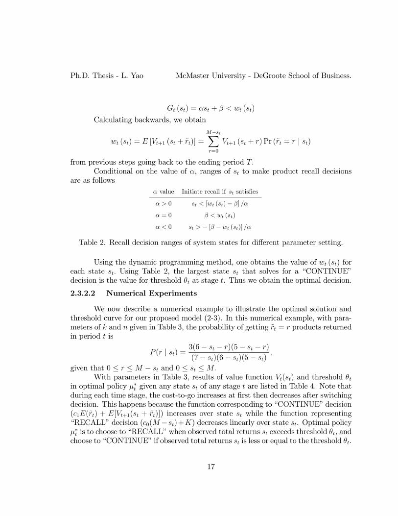
from previous steps going back to the ending period T.Conditional on the value of α, ranges of st to make product recall decisions
are as followsα value Initiate recall if st satisfies
α > 0 st < [wt (st)− β] /α
α = 0 β < wt (st)
α < 0 st > − [β − wt (st)] /α
Table 2. Recall decision ranges of system states for different parameter setting.
Using the dynamic programming method, one obtains the value of wt (st) foreach state st. Using Table 2, the largest state st that solves for a “CONTINUE”decision is the value for threshold θt at stage t. Thus we obtain the optimal decision.
2.3.2.2 Numerical Experiments
We now describe a numerical example to illustrate the optimal solution andthreshold curve for our proposed model (2-3). In this numerical example, with para-meters of k and n given in Table 3, the probability of getting rt = r products returnedin period t is
P (r | st) =3(6− st − r)(5− st − r)(7− st)(6− st)(5− st)
,
given that 0 ≤ r ≤M − st and 0 ≤ st ≤M.With parameters in Table 3, results of value function Vt(st) and threshold θt
in optimal policy µ∗t given any state st of any stage t are listed in Table 4. Note thatduring each time stage, the cost-to-go increases at first then decreases after switchingdecision. This happens because the function corresponding to “CONTINUE”decision(c1E(rt) + E[Vt+1(st + rt)]) increases over state st while the function representing“RECALL”decision (c0(M−st)+K) decreases linearly over state st. Optimal policyµ∗t is to choose to “RECALL”when observed total returns st exceeds threshold θt, andchoose to “CONTINUE”if observed total returns st is less or equal to the threshold θt.
17

Ph.D. Thesis - L. Yao McMaster University - DeGroote School of Business.
c0 c1 cF K n k M T
2 1 3 5 4 1 4 3
Table 3. Initial parameter values for the numerical example.
For instance, at period t equals 1, the optimal action is “CONTINUE”when observedtotal returns st is less or equal to 2 and optimal action switches to “RECALL”when stis greater or equal to 3; thus the largest observed returns st before switching decisionis 2, which is the threshold θ2.
Figure 2 shows optimal decisions for all states in every stage. The states forwhich optimal decision changes from “CONTINUE”to “RECALL”form the thresh-olds. Thresholds curve that reflects the optimal policy is shown as dark round dotsin Figure 2.
Changing the value of parameter K only while other parameters remain thesame in Table 3, the recall threshold θt varies as in Table 5. Recall threshold increasewhen immediate recall cost increase, which suggest high immediate recall cost dis-courages the action of product recalls. In our case, when immediate cost is higheror equal to 10, recall threshold is equal to 3 which equals M − 1; since recall actiononly take action when sT−1 = θT−1 + 1 for sT−1 <= M − 1, this result suggests thedecision maker will always choose to continue no matter how many products beingreturned.
Changing the value of parameter unit cost of goodwill cF only while otherparameters remain the same in Table 3, the threshold θt varies as in Table 6. Whenthe unit cost of goodwill cF decreases, recall threshold θt increases and the manageris less willing to recall. The unit cost of goodwill is the company’s estimation oflong-term impact of product returns to its reputation and customer loyalty. Themore a company cares about its market sustainability and long-term profit, the morecautious action it will take and the more willing it is to take a recall action.
When cF is within the range of [6, 11], the optimal decision for the first periodis “CONTINUE”. In contrast, when cF is within the range of [12,30], the optimaldecision for the first period is “RECALL”. Under this circumstance, the companyshould not release products in the first place.
2.3.2.3 Sensitivity Analysis
We experiment the impact of comparative magnitude of unit cost of managingreturn c1 and unit cost of recall c0 with four cases: (1) c0 c1, for instance c0 equals2 while c1 equals 20; (2) c0 < c1, for instance c0 equals 2 while c1 equals 5; (3) c0 > c1,for instance c0 equals 5 while c1 equals 2; (4) c0 c1, for instance c0 equals 20 whilec1 equals 2. The parameters settings are shown in Table 7.
18

Ph.D. Thesis - L. Yao McMaster University - DeGroote School of Business.
t st Vt(st) µ∗t θt t st Vt(st) µ∗t θt
0 0 8.54 CONTINUE 0 0 4.00 CONTINUE
0 6.74 CONTINUE 1 6.00 CONTINUE
1 7.80 CONTINUE 2 2 8.00 CONTINUE 2
1 2 8.60 CONTINUE 2 3 7.00 RECALL
3 7.00 RECALL 4 12.00 STOP
4 12.00 STOP
Table 4. Numerical experiment results of static rate recall timing problem.
Figure 2. Optimal decisions for all possible states and the threshold curve of thenumerical example of four products and three stages.
19

Ph.D. Thesis - L. Yao McMaster University - DeGroote School of Business.
K Corresponding threshold
1, . . . , 4 θt = 1 for t = 1, 2, 3
5, . . . , 8 θt = 2 for t = 1, 2, 3
9 θt =
2 t = 1
3 t = 2, 3
10 θt = 3 for t = 1, 2, 3
Table 5. Recall threshold increases with fixed recall cost K increases.
cF Corresponding threshold
1 θt = 3 for t = 1, 2, 3
2 θt =
2 t = 1, 2
3 t = 3
3 θt = 2 for t = 1, 2, 3
4, 5 θt = 1 for t = 1, 2, 3
6, . . . , 11 θt = 0 for t = 1, 2, 3
12, . . . , 30 θt = 0∗ for t = 1, 2, 3
Table 6. Recall threshold decreases with unit cost of goodwill increases.
Common parameters Case 1 Case 2 Case 3 Case 4
cF K n k M T c0 c1 c0 c1 c0 c1 c0 c1
3 15 100 1 10 12 2 20 2 5 5 2 20 2
Table 7. Other initial parameter values for numerical examples.
20

Ph.D. Thesis - L. Yao McMaster University - DeGroote School of Business.
Case 1. Optimal decisions of all possible states are shown in Figure 3 wherethe threshold curve plotted show a increasing trend of thresholds along with time.This is because the expected cost to continue decreases when there is less time left inthe warranty periods.
Figure 3. Optimal decisions of all possible states and the threshold curve in case 1:c0 c1 (c0 = 2, c1 = 20) .
Case 2. Optimal decisions of all states are plotted in Figure 4 where thethreshold curve also shows a increasing trend of thresholds with time. But the slopeis much more gentle compared to case 1 and the threshold at time t = 2 is higher.
Case 3. Optimal decisions of all states are plotted in Figure 5 where thethreshold curve shows a constant ratio of thresholds with time of t = 1, . . . , T − 1.Note the threshold curve of t = 1, . . . , T − 1 increases to θt = 8 compared to θt = 6in Case 2.
Case 4. Optimal decisions plotted in Figure 6 where the threshold curve showsa constant ratio of thresholds with time t = 1, . . . , T − 1 which are higher than theresults in previous three cases.
Our experiments in four cases show that thresholds are sensitive to the pa-rameter settings of unit cost of managing return c1 and unit cost of recall c0. Thesmaller c0 is relative to c1, the steeper the threshold curve as time increases. Oth-erwise, the thresholds line is flat and higher on the graph when c0 − c1 gets larger.These results suggest when recall costs increase faster than the return managing costfor “CONTINUE”decisions, managers tend to wait-and-see and take higher recallrisks.
21

Ph.D. Thesis - L. Yao McMaster University - DeGroote School of Business.
Figure 4. Optimal decisions of all possible states and the threshold curve in case 2:c0 < c1 (c0 = 2, c1 = 5) .
Figure 5. Optimal decisions of all possible states and the threshold curve in case 3:c0 > c1 (c0 = 5, c1 = 2) .
22

Ph.D. Thesis - L. Yao McMaster University - DeGroote School of Business.
Figure 6. Optimal decisions of all possible states and the threshold curve in case 4:c0 c1 (c0 = 20, c1 = 2) .
23
Ph.D. Thesis - L. Yao McMaster University - DeGroote School of Business.
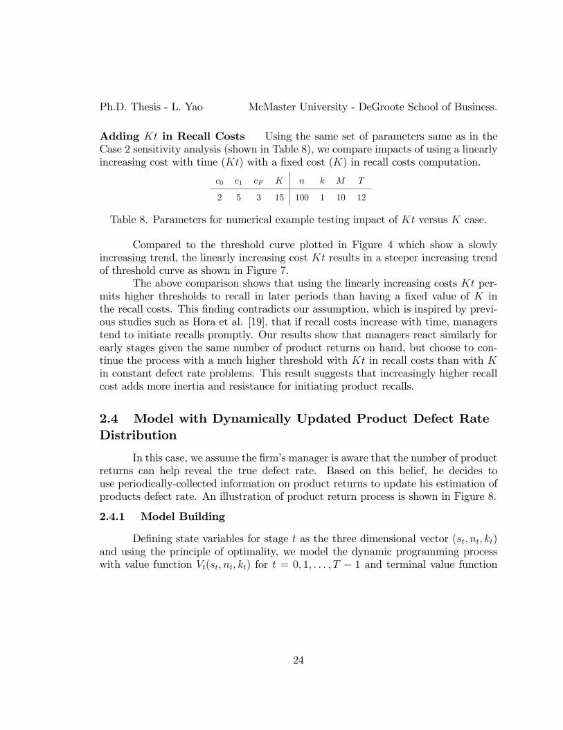
Adding Kt in Recall Costs Using the same set of parameters same as in theCase 2 sensitivity analysis (shown in Table 8), we compare impacts of using a linearlyincreasing cost with time (Kt) with a fixed cost (K) in recall costs computation.
c0 c1 cF K n k M T
2 5 3 15 100 1 10 12
Table 8. Parameters for numerical example testing impact of Kt versus K case.
Compared to the threshold curve plotted in Figure 4 which show a slowlyincreasing trend, the linearly increasing cost Kt results in a steeper increasing trendof threshold curve as shown in Figure 7.
The above comparison shows that using the linearly increasing costs Kt per-mits higher thresholds to recall in later periods than having a fixed value of K inthe recall costs. This finding contradicts our assumption, which is inspired by previ-ous studies such as Hora et al. [19], that if recall costs increase with time, managerstend to initiate recalls promptly. Our results show that managers react similarly forearly stages given the same number of product returns on hand, but choose to con-tinue the process with a much higher threshold with Kt in recall costs than with Kin constant defect rate problems. This result suggests that increasingly higher recallcost adds more inertia and resistance for initiating product recalls.
2.4 Model with Dynamically Updated Product Defect RateDistribution
In this case, we assume the firm’s manager is aware that the number of productreturns can help reveal the true defect rate. Based on this belief, he decides touse periodically-collected information on product returns to update his estimation ofproducts defect rate. An illustration of product return process is shown in Figure 8.
2.4.1 Model Building
Defining state variables for stage t as the three dimensional vector (st, nt, kt)and using the principle of optimality, we model the dynamic programming processwith value function Vt(st, nt, kt) for t = 0, 1, . . . , T − 1 and terminal value function
24

Ph.D. Thesis - L. Yao McMaster University - DeGroote School of Business.
Figure 7. Optimal decisions of all possible states and the threshold curve consideringrecall costs linearly increasing with time.
1 2 t t+10 T
r0 r1 rt
s0=0m0=M
s1=s0+r0m1=Ms1
s2=s1+r1m2=Ms2
st+1=st+rtmt+1=Mst+1
... ...
st=st1+rt1mt=Mst
k0n0
k1=k0+r0n1=n0+m0
k2=k1+r1n2=n1+m1
kt=kt1+rt1nt=nt1+mt1
kt+1=kt+rtnt+1=nt+mt
Figure 8. An illustration of product return process for dynamically updating productdefect rate model.
25

Ph.D. Thesis - L. Yao McMaster University - DeGroote School of Business.
VT (sT , nT , kT ) in expressions (8-9).
VT (sT , nT , kT ) = cF sT (8)
Vt(st, nt, kt) =
min
c0(M − st) +K Recall
c1E(rt | st, nt, kt)+ E[Vt+1(st+1, nt+1, kt+1)]
ContinueIf st < M
cFM Stop If st = M
(9)
where rt ∼ Bin(mt, pt) and pt ∼ Beta(kt, nt). Parameters are defined in Table 1.Definitions of value functions are similar to those of the constant defect rate model.The difference is the state space expands to three dimensional, i.e., (st, nt, kt), becauseknowledge of kt and nt are necessary to update the defect rate of stage t. As aconsequence, expected costs for returns management and the following periods areconditioned on the entire state space (st, nt, kt).
By the law of total probability, the probability of getting rt = r productsreturned in period t is
Pr(rt = r | st, nt, kt) =
∫ 1
0
Pr(r | p = p, st)fp(p | nt, kt) dp (10)
=
∫ 1
0
(M − st
r
)pr(1− p)M−st−rfp(p | nt, kt) dp
=Γ (r + kt) Γ (nt − kt +M − st − r) Γ (M − st + 1) Γ (nt)
Γ (M + nt − st) Γ (1 + r) Γ (M − st − r + 1) Γ (kt) Γ (nt − kt)whose complexity contributes to the solving diffi culty of the dynamically updateddefect rate problem. Gamma function Γ (n) is an extension of factorial functionswhere
Γ (n) =
∫ ∞0
xn−1e−xdx
and Γ (n) = (n− 1)! if n is an integer. Applying the law of total probability, similarto the computing steps in finding c1E(rt) for the constant rate model with formula(4), we have
c1E(rt | st, nt, kt) = c1ktnt
(M − st) . (11)
2.4.1.1 Conjugate property of beta distribution and Bernoulli trials
Suppose in period t the return rate pt follows a beta distribution with para-
26

Ph.D. Thesis - L. Yao McMaster University - DeGroote School of Business.
meters kt and nt (kt ≤ nt), i.e., pt ∼ Beta(kt, nt) for which the expectation E(pt) iskt/nt. At the first stage (t = 0), prior estimation of return rate follows Beta(k0, n0)for which parameters k0 and n0 are exogenously determined by historical data or thedecision maker. The number of products remaining in market mt and the total num-ber of returned products st follows the relationship that mt + st = M as mentionedpreviously. The number of product returns in period t follows a binomial distribu-tion since the process is similar to conducting mt identical Bernoulli processes withsuccess rate pt, i.e., rt ∼ Bin(mt, pt). The conjugate property of beta distributionsand Bernoulli processes states that if the prior distribution follows a beta distribu-tion Beta(r, n) and the sampling process is Bernoulli with r′ successes out of n′ trialsthen the posterior distribution also follows a beta distribution Beta(r′′, n′′) wherer′′ = r + r′, n′′ = n + n′. Winkler [53] provides excellent materials on the conjugateproperty for those interested, covering proofs and examples. In our case, with initialestimation following a beta distribution and all sampling processes being Bernoulli,we can prove by induction that the resulting posterior distributions are also betadistributions.
With the conjugate property of beta distribution and Bernoulli trials, the sys-tem states for the dynamically updated defect rate model update using the followingrecursive expressions for any t = 1, 2, . . . , T.
kt+1 = kt + rt (12)nt+1 = nt + (M − st) (13)
Therefore given system state (st, nt, kt) at stage t, we can solve for the expected costsof stages starting from t+ 1 using expression (14).
E[Vt+1(st+1, nt+1, kt+1)] =M−st∑r=0
Vt+1 (st + r, nt +M − st, kt + r) Pr(rt = r | st, nt, kt).
(14)
2.4.1.2 Applying Conjugate Property to States kt and nt
Since the total number of returned products at the beginning of period t isst =
∑t−1i=1 ri, for t = 1, 2, . . . , T −1 and s1 = 0, parameters kt and nt have expressions
in the following.
kt =
k0 t = 0
k0 + st t = 1, 2, . . . , T − 1(15)
27

Ph.D. Thesis - L. Yao McMaster University - DeGroote School of Business.
nt =
n0 t = 0
n0 + tM −∑t−1
i=0 si t = 1, 2, . . . , T − 1(16)
=
n0 t = 0
n0 +M t = 1
n0 + tM −∑t−2
i=0(t− 1− i)ri t = 2, 3, . . . , T − 1
(17)
We can prove formulas for kt and nt by induction.Proof. Since k0 is given, k1 = k0+r0 satisfies the form kt+1 = k0+
∑ti=0 ri. Suppose
this formula holds for any ` that 1 ≤ ` ≤ T − 1, i.e., k` = k0 +∑`−1
i=0 ri. Then
k`+1 = k` + r`
= k0 +`−1∑i=0
ri + r`
= k0 +∑i=0
ri
also satisfies the proposed formula.For the formula of nt with respect to system states, with n0 given n1 = n0 +
m0 = n0 +M − s0 which satisfies the formula nt = n0 + tM −∑t−1
i=0 si. Suppose thisformula holds for any ` that 1 ≤ ` ≤ T − 1, i.e., n` = n0 + `M −
∑`−1i=0 si. Then
n`+1 = n` +m`
= n0 + `M −`−1∑i=0
si +M − s`
= n0 + (`+ 1)M −∑i=0
si
also satisfies the proposed formula.For the formula of nt with respect to returns in previous stages, with n0 given,
n1 = n0 +m0 = n0 +M , n2 = n1 +m1 = n0 +M + (M − r0) = n0 + 2M − r0 whichsatisfies the formula nt = n0 + tM −
∑t−2i=0(t − 1 − i)ri. Suppose this formula holds
28

Ph.D. Thesis - L. Yao McMaster University - DeGroote School of Business.
for any ` that 2 ≤ ` ≤ T − 1, i.e., n` = n0 + `M −∑`−2
i=0(`− 1− i)ri. Then
n`+1 = n` +m`
= n0 + `M −`−1∑i=0
si +M − s`
= n0 + (`+ 1)M −∑i=0
si
also satisfies the proposed formula.For the formula of nt with respect to returns in previous stages, with n0 given,
n1 = n0 +m0 = n0 +M , n2 = n1 +m1 = n0 +M + (M − r0) = n0 + 2M − r0 whichsatisfies the formula nt = n1 + (t − 1)M −
∑t−2i=0(t − 1 − i)ri. Suppose this formula
holds for any ` that 3 ≤ ` ≤ T , i.e., n` = n1 + (`− 1)M −∑`−2
i=0(`− 1− i)ri. Then
n`+1 = n` +m`
= n0 + `M −`−2∑i=0
(`− 1− i)ri + (M −`−1∑i=0
ri)
= n0 + `M −`−2∑i=0
(`− 1− i)ri + (M −`−2∑i=0
ri − r`−1)
= n0 + (`+ 1)M −`−1∑i=0
(`− i)ri
also satisfies the proposed formula. By induction, we show the formulas (15), (16)and (17) hold for t = 2, 3, . . . , T − 1.
2.4.1.3 Identifying State Space
The notion of “curse of dimensionality”was coined by Bellman [5]. This innatefeature is as old as the technique of dynamic programming itself. Exponentiallyincreasing state space makes the calculation for value functions very diffi cult, if notimpossible, when the problem size increases. To deal with this curse, researchers suchas Powell [35] apply approximation methods to constrain the exploding dimensions.Powell [35] categorizes three types of curse of dimensions, including state space, actionspace and decision space.
Fortunately, in our problem we can reduce the dimensionality by observing theconnections of states st, nt and kt. Given the number of product returns until time t,i.e., st, beta distribution parameter kt is decided by k0+st for all t = 0, 1, 2, . . . , T −1
29

Ph.D. Thesis - L. Yao McMaster University - DeGroote School of Business.
since s0 = 0, but nt could be a range if time t is at stage 2 or after. Using nt and ntto denote the lower and upper bound of the range for nt, then
nt = n0 + tM, ∀t ≥ 2 (18)
when si = 0 for all i = 1, 2, . . . , t− 1.
nt = n0 + tM − (t− 1)st, ∀t ≥ 2 (19)
when r0 = st and ri = 0 for all i = 1, . . . , t− 2, i.e., si = st, for all i = 1, . . . , t− 1.
nt = min n0 + tM −t−2∑i=0
(t− 1− i)ri (20)
subject tot−2∑i=0
ri ≤ st
0 ≤ ri ≤M − si, ∀i = 0, . . . , t− 2k−1∑i=0
ri ≤ st, ∀k = 1, . . . , t− 1
s0 = 0
ri ∈ N+, ∀i = 0, . . . , t− 2
To explain the proposed lower bound in expression (19), we present the system(20) that minimizes nt defined in expression (17) as the objective and in its constraintsconfine product return ri (∀i = 0, . . . , t − 2) following the updating rules. Becausefunction
∑t−2i=1(t− 1− i)ri is a weighted sum of non-negative decision variables ri, its
minimum can be found by assigning the decision variable that has the largest weight,i.e., r0, with its largest possible value st and the rest of ri to be zero. If we changethe minimum in the objective to maximum, then the revised version of system (20)will find the upper bound of nt in expression (18). The maximum can be found whenassigning ri (∀i = 0, . . . , t−2) to be zero, in which case the number of product returnsof the first t− 1 periods is always zero.
Hence given time t ≥ 2, the state space is bounded separately with st ∈ [0,M ],kt = k1 + st, and nt ∈ [n1 + tM − (t − 1)st, n1 + tM ]. The range of st is M + 1,kt depends on st, and the range of nt is (t − 1)st + 1. Thus given st, the number ofproducts returned at stage t = 2, 3, . . . , T , there are (t−1)st+ 1 corresponding states(st, nt, kt) in the dynamically updated product defect rate distribution model.
2.4.2 Solution using Dynamic Programming
Similar to solving the fixed defect rate model, we apply dynamic programming
30

Ph.D. Thesis - L. Yao McMaster University - DeGroote School of Business.
to solve the dynamic updating defect rate model (8-9). Because the state spaceextends from st to (st, kt, nt), we calculate the value function based on the rangesof kt from expression (15) and nt from expression (16). In this backward inductionprocess, we use the conjugate property of the beta distribution and Bernoulli trialsfor states updating and compute the transition probability with expression (10) tofind the value of cost-to-go (14).
Comparing the results of taking “RECALL”action with immediate recall costsand taking “CONTINUE” action with the expected expenditure of cost-to-go, weobtain the optimal decisions for each possible state at all stages. Since the state sthas much more impact than the states kt and nt, we use the concept of thresholdsdefined for the fixed rate model, i.e., threshold θt is the largest state st that the“CONTINUE”decision remains optimal at stage t. Thresholds of all stages comprisethe optimal policy.
2.4.2.1 The threshold curve
Similar to our study approach for the constant defect rate model, we start byexamining the threshold from the last period θT−1 to gain some insight of DP solvingprocedures.
Proposition 2 Product recall threshold for the last time period is determined bygiven parameters from Table 1 and beta parameters k and n with following equation:
θT−1 =
⌊K + [c0 − (c1 + cF ) kT−1/nT−1]M
(1− kT−1/nT−1) cF + c0 − c1k/n
⌋(21)
Proof. The definition of recall threshold, θT−1 is the largest number of return that“CONTINUE”remains the optimal decision, i.e., the cost to continue is equal to orless than the cost to recall. From the model (2-3), certain states sT−1 satisfy thefollowing inequality
c0 (M − sT−1) +K ≥ c1E (rT−1) + E [VT (sT−1 + rT−1)]
From analysis in (4), we can writeE (rT−1) = kT−1/nT−1 (M − sT−1), therefore
c0 (M − sT−1) +K ≥ c1kT−1nT−1
(M − sT−1)
+E
[VT
(sT−1 +
kT−1nT−1
(M − sT−1))]
[(1− k
n
)cF + c0 − c1
kT−1nT−1
]sT−1 ≤ K +K +
[c0 − (c1 + cF )
kT−1nT−1
]M
31

Ph.D. Thesis - L. Yao McMaster University - DeGroote School of Business.
It is reasonable to assume that unit cost incurred during a recall is higherthan that for managing returns in a “CONTINUE” decision, i.e., c0 > c1. Theratio kT−1/nT−1 is equivalent to the expectation of defect probability E(p), 0 <kT−1/nT−1 < 1. Hence the coeffi cient of sT−1 is positive, and we can solve the aboveinequality for all eligible sT−1.
sT−1 ≤K + [c0 − (c1 + cF ) kT−1/nT−1]M
(1− kT−1/nT−1) cF + c0 − c1kT−1/nT−1Because recall threshold corresponds to the largest eligible sT−1 solved, the
result in (21) holds.Now extend the above procedure to compute thresholds prior to the last peri-
ods. When 0 ≤ st ≤M −1 for t = 2, . . . , T −1, let function A (st, nt, kt) denote recallcosts c0 (M − st) +K, function wt (st, nt, kt) denote expected costs for all future peri-ods if continue E [Vt+1 (st + rt, nt +M − st, kt + rt)], and functionB (st, nt, kt) denotereturn management costs c1E (rt | st, nt, kt) which equals to c1 (M − st) kt/nt, valuefunction transforms to the following:
Vt (st, nt, kt) = min
A (st, nt, kt)
B (st, nt, kt) + wt (st, nt, kt)
The company initiates recall only if A (st, nt, kt) < B (st, nt, kt)+wt (st, nt, kt).Let function Gt (st, nt, kt) refer to the difference between recall costs and return man-agement costs, i.e.,
Gt (st, nt, kt) = A (st, nt, kt)−B (st, nt, kt)
=
(c1ktnt− c0
)st +
(c0 − c1
ktnt
)M +K
= αkt,ntst + βkt,nt
where α (kt, nt) = c1kt/nt − c0 and β (kt, nt) = (c0 − c1kt/nt)M + K. Consequently,the firm initiates product recall only when
Gt (st) = α (kt, nt) st + β (kt, nt) < wt (st, nt, kt)
Calculating backwards, with expression (14) we obtain
wt (st, nt, kt) = E [Vt+1 (st + rt, nt +M − st, kt + rt)]
=M−st∑rt=0
Vt+1 (st + rt, nt +M − st, kt + rt) Pr (rt | st, nt, kt)
32

Ph.D. Thesis - L. Yao McMaster University - DeGroote School of Business.
from previous steps going back to the ending period T.Theoretically, given each system state (st, nt, kt), we can compute the corre-
sponding α (kt, nt) and β (kt, nt) . Conditional on the value of α (kt, nt), ranges of stto make product recall decisions are as follows
α (kt, nt) value Initiate recall if st satisfies
α (kt, nt) > 0 st < [wt (st, nt, kt)− β (kt, nt)] /α (kt, nt)
α (kt, nt) = 0 β (kt, nt) < wt (st, nt, kt)
α (kt, nt) < 0 st > − [β (kt, nt)− wt (st, nt, kt)] /α (kt, nt)
Table 9. Recall decision ranges of system state st for dynamically changing defectrate model.
2.4.2.2 Numerical experiments
We experiment with a numerical example using the parameters in Table 10 andfind results shown in Figure 9. The solid circle dots indicate the optimal decisionsto “CONTINUE”, the cross dots indicate the decision to “RECALL”, the emptydiamond dots indicate the decision to “STOP”and solid square dots indicate thatdecisions depend on nt state.
The generic model considers a larger state space in which the current stateis determined not only by the number of products returned so far, i.e., st, but alsohow these products were returned through time, i.e., nt. Hence, with the same prod-ucts returned, the optimal decisions could be either “CONTINUE”or “RECALL”depending how the returned products were accumulated. The decision in this case isidentified as “nt-DEPENDENT”, because the manager cannot make a decision basedon the number of products returned alone, he also needs the return history which isreflected by nt.
We increase the number of time stages T from 4 (Figure 9) to 8 (Figure 10), 12(Figure 11) and 16 (Figure 12) to identify its impact on optimal decisions and thresh-old curve. With larger problem sizes, the situation of “nt-DEPENDENT”appearsmore frequently at the borders between regions of “CONTINUE”and “RECALL”decisions. For example when T is 4, only one “nt-DEPENDENT”dot shows for t = 2and st = 9. Detailed results show when the state is in (s2 = 9, 21 ≤ n2 ≤ 26, k2 = 10),we choose “RECALL”; when the state is in (s2 = 9, 27 ≤ n2 ≤ 30, k2 = 10), we choose“CONTINUE”. In contrast, we have three “nt-DEPENDENT”states for T = 8, fourand six “nt-DEPENDENT”states for T = 12 and T = 16 respectively.
Comparing the four results in Figures 9-12, it appears that, with the same costparameters, the threshold curve shifts up with more initial products in the market.
33
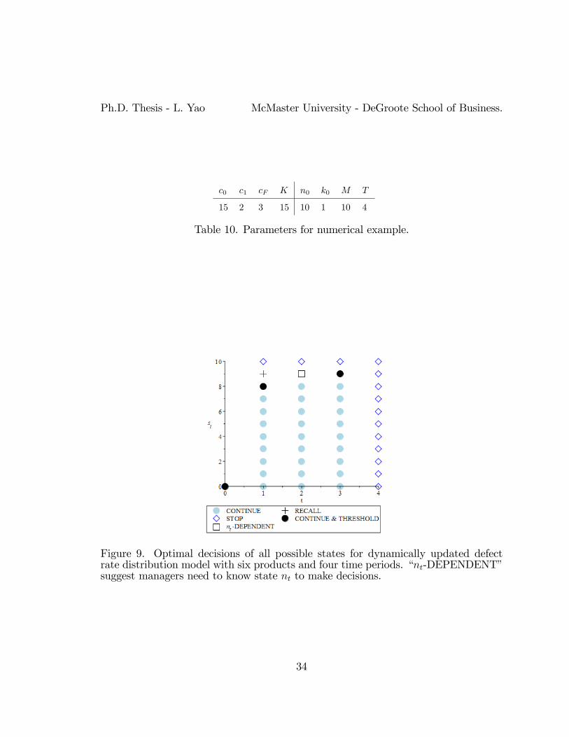
Ph.D. Thesis - L. Yao McMaster University - DeGroote School of Business.
c0 c1 cF K n0 k0 M T
15 2 3 15 10 1 10 4
Table 10. Parameters for numerical example.
Figure 9. Optimal decisions of all possible states for dynamically updated defectrate distribution model with six products and four time periods. “nt-DEPENDENT”suggest managers need to know state nt to make decisions.
34

Ph.D. Thesis - L. Yao McMaster University - DeGroote School of Business.
Figure 10. Optimal decisions of all possible states for dynamically updated defectrate distribution model with six products and eight time periods. “nt-DEPENDENT”suggest managers need to know state nt to make decisions.
35

Ph.D. Thesis - L. Yao McMaster University - DeGroote School of Business.
Figure 11. Optimal decisions of all possible states for dynamically updated defectrate distribution model with six products and 12 time periods. “nt-DEPENDENT”suggest managers need to know state nt to make decisions.
States with “nt-DEPENDENT”optimal decisions appear as the intermediate statesat the inflection points when threshold curve rises up. For these states, completeknowledge of the states (st, nt, kt) is required to make optimal decisions.
2.4.3 Size of State Space
Using results of identifying dimensionality, based on the range of nt there are(t− 1)st + 1 corresponding states (st, nt, kt) for any given st at stage t = 2, 3, . . . , T .For any stage t = 2, 3, . . . , T, the number of states is
M∑st=0
[(t− 1)st + 1] = M + 1 +
M∑st=0
(t− 1)st
= M + 1 + (t− 1)
M∑st=0
st
= M + 1 + (t− 1)M (M + 1)
2.
36

Ph.D. Thesis - L. Yao McMaster University - DeGroote School of Business.
Figure 12. Optimal decisions of all possible states for dynamically updated defectrate distribution model with six products and 16 time periods.“nt-DEPENDENT”suggest managers need to know state nt to make decisions.
37

Ph.D. Thesis - L. Yao McMaster University - DeGroote School of Business.
The number of states for all stages since the second stage is
T∑t=2
M∑st=0
[(t− 1)st + 1] =T∑t=2
[M + 1 + (t− 1)
M (M + 1)
2
]
= (M + 1) (T − 1) +M (M + 1)
2
T∑t=2
(t− 1)
= (M + 1) (T − 1) +M (M + 1)
2
T (T − 1)
2
= (M + 1) (T − 1)
(1 +
MT
4
)=
1
4
(M2T 2 −M2T +MT 2 + 3MT − 4M + 4T − 4
).
Adding the number in the first stage, which is one, and the number in second stage,which isM+1, the total number for states a dynamically updated defect rate problemwith given initial products on market M and warranty time span T , is
T∑t=2
M∑st=0
[(t− 1)st + 1] + 1 +M + 1 =1
4
(M2T 2 −M2T +MT 2 + 3MT + 4T
)+ 1.
This number largely depends on the value M2T 2/4 when M and T get large.For instance, when M equals 100 and T equals 24, the number of possible statesis 1,396,225 which is close to 1,440,000, the result of M2T 2/4. Since the number ofstates rapidly increases whenM and T get large, the computation for value functionsbecomes increasingly time consuming, which motivates us to develop alternatives tofind the optimal solutions.
2.4.4 Simulation Method
To avoid the time-consuming computation of the value function Vt(st, kt, nt),we use the simulation method to directly find the best fitting curve for product recallthresholds. Results from our previous numerical example indicate that the thresholdscurve can be deemed to be a function of time stages. To be specific, the thresholdscurve shows a nondecreasing trend as time stage t increases. A general function formof
θt = an√t
could be used for nonnegative parameters a and n. For simplicity, we use threefunctional forms: linear functions (n = 1), square root functions (n = 2) and cu-
38

Ph.D. Thesis - L. Yao McMaster University - DeGroote School of Business.
bic root functions (n = 3) to approximate this relationship between thresholds andtime stages. Thus we transform the process of finding thresholds into optimizingparameters in the approximation functions.
Given any of the three functional forms, the largest slope is defined when thethreshold of the second stage (t = 1) reaches M − 1 because the process terminateswhen system state reaches M . Thus feasible ranges for slope a is [0,M − 1] . Wecan limit the selection of parameter a to a range of equidifferent integers to show itsimpact on the objective.
After choosing a functional form, we use randomly generated states to evaluatethe total cost when applying a certain value of the parameter a in the function.Comparing among all candidates, the best choice of a completes the approximationfunction and provides thresholds of all time stages.
A benefit of adopting this simulation method is that we can ignore the com-plexity of computing value functions for all possible states in each time stage. Thismethod also works for the dynamically distributed defect rate model if we are willingto sacrifice some accuracy in system states.
Globally optimizing the simulation method requires the model to satisfy acertain level of convexity, for instance, the golden section method requires quasi-convexity. The trait of convexity is hard to prove for our models. Therefore, wewill adopt an approaching method of using discretized values of a from its applicablerange. For example, if we choose an equal interval of 0.5 and suppose M equals 11,then the candidates of a are 0, 0.5, 1, 1.5, . . . , 9.5, 10. For each candidate, we runthe simulation for a suffi cient amount of trials so that the sample mean is reliable.
In stage t of a simulation trial with given system states (st, kt, nt), we firstjudge whether the system should “RECALL”or “CONTINUE”by comparing st andθt. If st is greater than θt, which means “RECALL” is the better choice, then wecompute the immediate recall costs and add it to the total costs and end its trial.Otherwise, if st is less than or equal to θt, we make a “CONTINUE”decision andupdate the system as follows. We start by generating the probability for any productin the market failing during this time period, i.e., product defect rate of this stage.This probability pt follows the beta distribution. We use the uniformly distributedrandom number U generated by the computer as the cumulative probability from 0to pt with the beta distribution.∫ pt
0
(nt − 1)!
(kt − 1)!(nt − kt − 1)!pkt−1(1− p)nt−kt−1dp = U (22)
Solving expression (22) for the probability pt prepares the calculation for the numberof returns rt in this stage. Since rt follows a binomial distribution of mt products inthe market, which equals M − st, and event occurrence rate of pt, we use another
39

Ph.D. Thesis - L. Yao McMaster University - DeGroote School of Business.
c0 c1 cF K n0 k0 M T
15 10 3 15 10 1 16 16
Table 11. Parameter settings for the simulation example.
random number as the accumulative probability following Binomial distribution andobtain rt. Based on system states and rt, we compute the return management costof this stage and add it to the total costs. Following the states updating formulas(12-13), we now obtain the states (st + rt, kt + rt, nt + (M − st)) as (st+1, kt+1, nt+1)for stage t + 1 and are ready for the next stage. The process terminates when allproducts are returned or it reaches the ending stage, and a termination cost incursfor both cases.
Comparing the mean of total costs for all the candidates, we select the onewith the smallest costs and use it for the thresholds curve. The simulation methodrequires much less computation because the number of parameter candidates increaseswith total products numberM alone, compared to the complexity of using DP whichincreases with M2T 2.
2.4.4.1 Exact Solution and Comparison
We can show the effi ciency of using the simulation method with a numericalexample. Using the parameters as shown in Table 11, we calculated the optimalsolutions shown in Figure 13 with dynamic programming. The expected total cost(V0) is 127.60 from our DP computation.
We select the value candidates for parameter a from the set 1, 3, 5, 7, 9 andaim to test the effi ciency of approximation, explore the best fitting function and findthe best parameter choice for each functional form. First, we approach the thresholdcurve with linear functions
θt = at.
With repetition number of 5000, our simulation results are shown in Table 12.We use the percentage of error instead of effi ciency since the former shows a
better trend. The error is defined as the percentage difference between the simulationaverages (E (TC)) and expected cost calculated using dynamic programming (V0).
Error(%)=V0 − E (TC)
V0· 100%
Our linear function approximation results show a = 5 as the best choice with thelease error of 4.73%.
We also use the 95% confidence interval (CI) to complement our point esti-
40

Ph.D. Thesis - L. Yao McMaster University - DeGroote School of Business.
Figure 13. Optimal solutions calculated with dynamic programming method for adynamically updating defect rate distribution model with parameters in Table 11.
a 9 7 5 3 1
E (TC) 135.41 134.54 133.64 138.23 167.04
Error 6.12% 5.43% 4.73% 8.33% 30.91%
95%CI-LB 133.59 132.75 131.81 136.29 164.60
95%CI-UB 137.22 136.32 135.47 140.17 169.48
Table 12. Simulation results with linear function approximations (θt = at), wherea = 5 is the best choice with the smallest error rate for problem parameters given inTable 11.
41

Ph.D. Thesis - L. Yao McMaster University - DeGroote School of Business.
Figure 14. Combining DP solved optimal results with approximating linear functions(θt = at), where a = 5 is the best choice with the smallest error rate for problemparameters given in Table 11.
mation of expected cost (E (TC)). The lower bound (LB) and upper bound (UB) ofthe confidence interval in Table 12 are calculated with the following formula
LB = µ− tα/2s√n, UB = µ+ tα/2
s√n
where µ and s are the mean value and sample standard deviation of our experimentresults respectively; since our experiment repetition n is 5000, we use zα/2 of 1.96instead of the t distribution value.
Combining the linear function lines with the threshold curve and optimal so-lutions results in Figure 14. The number of states violating the DP optimal resultsis the least when a = 5 in linear approximations is perhaps the reason why it showsthe least error percentage.
Next, we experiment the square root functions
θt = a√t
with the same set of values 1, 3, 5, 7, 9 as the candidates for parameter a. In Table13, experiment results show the square root function performs the best when a = 7with error equals 3.88%. Observing the combination of all five square root functioncurves and the DP solved optimal solutions in Figure 15, the curve using a = 7 hasperhaps the least number of states violating the optimal decisions from DP solution.
42

Ph.D. Thesis - L. Yao McMaster University - DeGroote School of Business.
a 9 7 5 3 1
E (TC) 134.46 132.55 133.00 151.11 210.04
Error 5.37% 3.88% 4.23% 18.42% 64.61%
95%CI-LB 132.67 130.74 131.16 148.92 207.97
95%CI-UB 136.25 134.36 134.84 153.29 212.21
Table 13. Simulation results with square root function approximations (θt = a√t),
where a = 7 is the best choice with the smallest error rate for problem parametersgiven in Table 11.
Figure 15. Combining DP solved optimal results with approximating square rootfunctions (θt = a
√t), where a = 7 is the best choice with the smallest error rate for
problem parameters given in Table 11.
43

Ph.D. Thesis - L. Yao McMaster University - DeGroote School of Business.
a 9 7 5 3 1
E (TC) 133.41 132.92 138.42 170.77 216.71
Error 4.55% 4.16% 8.48% 33.83% 69.84%
95%CI-LB 131.59 131.16 136.43 168.44 214.79
95%CI-UB 135.22 134.67 140.41 173.10 218.64
Table 14. Simulation results with cubic root function approximations (θt = a 3√t),
where a = 7 is the best choice with the smallest error rate for problem parametersgiven in Table 11.
Then we experiment with cubic root functions
θt = a3√t
with the same value set for parameter a. The simulation results shown in Table 14present a = 7 as the best choice for cubic root functions with error 4.16%. Alsocombining the cubic function curves and DP-obtained optimal results in Figure 16confirms our observation that the best fitting curve has the least states violatingoptimal decisions.
Comparing all of the above results, the square root function using parametera = 7 has the least error percentage. Therefore, we choose the square root functionθt = a
√t for simulations of large size problems.
2.4.4.2 Estimation of Threshold Curve for Large Scale Problems
We exemplify the effi ciency of using simulation method with the setting thatproducts number M is 100 and time stages T is 24. In this case the total number ofstates approaches 1.4 million as discussed in Section 2.4.3.
Since the number of products increases to 100, we choose the candidates forparameter a from the set 10, 30, 50, 70, 90 . Our computation results shows in Table16 using 5000 repetitions for each parameter candidate. The results suggest thatusing a = 50 in the square root function has the lowest expected costs 944.90, whichcan be used as the upper bound estimation for expected costs. Our simulation with5000 repetitions takes about 300 seconds (five minutes) to finish, yet applying the DPmethod takes over 361,200 seconds (above 100 hours) to finish.
Note that our simulation results provide the best choice within the given can-didates. It is likely that in between these numbers there are better choices of thefunction parameter for more accurate approximation. The limitation of simulationcomes from both the choice of functional form and the choice of parameter candi-dates set. The benefits of using simulation include a guaranteed solution and quick
44

Ph.D. Thesis - L. Yao McMaster University - DeGroote School of Business.
Figure 16. Combining DP solved optimal results with approximating cubic rootfunctions (θt = a 3
√t), where a = 5 is the best choice with the smallest error rate for
problem parameters given in Table 11.
c0 c1 cF K n0 k0 M T
15 10 3 15 100 1 100 24
Table 15. Parameter settings for the large size problem (M = 100, T = 24) inassessing the simulation method.
a 90 70 50 30 10
E (TC) 951.93 950.87 944.90 945.70 1155.78
95%CI-LB 941.51 940.52 934.53 935.47 1143.08
95%CI-UB 962.34 961.21 955.27 955.92 1168.47
Time(sec.) 301 301 299 270 96
Time(min.:sec.) 5:01 5:01 4:59 4:30 1:36
Table 16. Simulation results for large size problem (M = 100, T = 24) with squareroot function approximations (θt = a
√t), where a = 50 is the best choice with the
smallest expected costs for problem parameters given in Table 15.
45
Ph.D. Thesis - L. Yao McMaster University - DeGroote School of Business.
response to the change of problem settings, which can provide the decision maker areliable approach for examining different problem scenarios and a dependable upperbound estimation of expected costs.
2.5 Conclusions and Proposal for Future Research
In this chapter, we construct the model for making product recall decisionsby using the number of product returns to update the estimation of product defectrate distribution. Our primary contribution to the literature is that we model andsolve the optimization problem of product recalls by combining dynamic programmingwith the Bayesian conjugate property of beta distributions and Bernoulli processes.We build two models of different defect rate distribution estimation. The model forstationary defect rate distribution assumes the random variable for defect rate followsthe same distribution during the entire time horizon, while the dynamically updatingdefect rate distribution uses the product returns of the proceeding stage to updatethe estimated distribution.
We define the threshold curve as the connection of states of largest number oftotal returns of all stages in the optimal solution. The threshold curve for the optimaldecision shows a nondecreasing trend that crosses the origin. This observation inspiresour approximation of the threshold curve by nonlinear functions, such as square rootfunctions and cubic root functions.
Our proposed DP method is capable of solving moderate sized problems andobtaining optimal solutions of all possible states. Yet, the computation complexityis proportion to the squared product of the number of products in the market andtotal time stages. Therefore we apply the simulation method for problem-solving,which shows low-error rate performance when applied to moderate-size benchmarkproblems. Our experiments show the proposed simulation method could solve thelarge sized problems in a satisfying balance of solution accuracy and computationtime.
In future work, we propose to explore the feasibility of using approximate dy-namic programming methods to solve our model. Unlike the backward recursion usedin dynamic programming, the Approximate Dynamic Programming (ADP) steps for-ward through time using value function approximation and sample paths in search ofthe optimal solution. Sample path is a sequence of exogenous information that de-scribes the stage transitions of all defined stages. ADP implements suffi cient amountof calculation iterations using sample paths to find the satisfactory approximation forvalue functions.
A commonly used method to approximate the value function is Q-learning.Application of Q-learning for optimal stopping problem has been discussed by Bert-
46

Ph.D. Thesis - L. Yao McMaster University - DeGroote School of Business.
sekas and Tsitsiklis [7] where the transitional probability matrix is given and hasa steady-state distribution. Based on their work, we may be able to explore thepossibility of applying Q-learning to our dynamically updated product defect ratedistribution model.
47

Ph.D. Thesis - L. Yao McMaster University - DeGroote School of Business.
Chapter 3Newsvendor Problem using Quality In-vestment for Product Recall Risk Control
This chapter extends the classic single-period stochastic newsvendor modelwith product recall risk management. The probability of product recalls is capturedby a decreasing function of product quality level. The core company exerts control onproduct quality through manufacturing investment, which impacts unit productioncost, to optimize total expected profits. Given the free choices of the cost func-tion and recall probability function, the resulting objective function considering salerevenues, operational costs and recall risks is not necessarily negative semi-definite.Parametric analysis in the newsvendor model reveals several interesting features. Oneis that the production quantity and quality level seem to have conflicting effects asone waxes and the other wanes in optimal solutions during most cases of parame-ter changes. The only two exceptions include changing variable unit production costand demand rate. Another feature is that increasing profitability discourages invest-ment in quality. We further extend our model from internal supply to external supplyfrom multiple sources. In the case of two external suppliers satisfying independentdemands and covering each other’s demand only when the other is having recalls,our results suggest little impact from recall-covering interaction on optimal solutions.Additional numerical results show consistency with internal supply case.
3.1 Introduction
This chapter extends the newsvendor problem with product quality control.In order to deal with risks in product recall, the core company decides its invest-ment level on product quality, which impacts production cost and the probabilityof product recall. The classic newsvendor problem is a single-period stochastic in-ventory control problem. In their influential work, Arrow, Harris and Marschak [2]examine the newsvendor model and derive the critical fractile solution. We follow thesame notation system in Parlar [32] which provides an excellent detailed review of theproblem. Typically it considers seasonal products for which leftover products havelittle value – the salvage value is small compared to the sale price. Through decid-ing the optimal order quantity Q the newsvendor model considers the expected totalprofit that includes salvage values (v per unit), penalty costs (p per unit), sales rev-
48

Ph.D. Thesis - L. Yao McMaster University - DeGroote School of Business.
enue (s per unit) and purchasing costs (c per unit). Suppose the demand is denotedby random variable X with a probability density function f(x), the random profit isdenoted by Π and a realized value of profit π can be written as
π =
sx+ v(Q− x)− cQ, if x ≤ Q (surplus)
sQ− p (x−Q)− cQ, if x > Q (shortage)
Thus, the expected profit E [Π] = P (Q) is a function of order quantity:
P (Q) =
∫ Q
x=0
[sx+ v(Q− x)− cQ] f (x) dx
+
∫ ∞x=Q
[sQ− p (x−Q)− cQ] f (x) dx
= (s− v)µ− (c− v)Q− (s+ p− v)
∫ ∞x=Q
(x−Q) f (x) dx
where µ = E [X] is the mean demand. Using Leibniz’s rule of differentiation, we have
P ′ (Q) = −(c− v) + (s+ p− v)
∫ ∞x=Q
f (x) dx
P ′′ (Q) = − (s+ p− v) f (Q) ≤ 0
and the negative second order derivative proves the objective function concave.The concavity of the above objective function leads us to solve the problem
with first and second order optimality conditions. Given the demand probabilitydensity function f (x) and using F (x) for the corresponding cumulative distributionfunction (CDF), one can obtain the optimal order quantityQ∗ by solving the followingequation
F (Q∗) =
∫ ∞x=Q
f (x) dx =c− v
s+ p− vwhere F (x) = 1− F (x) .
The newsvendor model assumes products have perfect quality, however, recentproduct recall events suggest otherwise. We consider possible product recalls, whichoccur after product sales, in response to low product quality. The core company con-trols product quality through investment in manufacturing; high investment ensureshigh product quality level. We use ` to denote product quality level and R(`) todenote the probability of incurring a product recall because of quality concerns. Im-proving quality level ` decreases the product recall probability R(`) (0 ≤ R(`) ≤ 1)and increases the unit cost of production, denoted by c(`). Hence, first derivative
49

Ph.D. Thesis - L. Yao McMaster University - DeGroote School of Business.
functions satisfy the following conditions:
R′(`) =dR (`)
d`< 0, c′(`) =
dc (`)
d`> 0
By choosing the right manufacturing quantity Q and quality level ` we can maximizethe expect total profits, denoted by E(Π), considering revenues, operational costs,and possible recall costs. Product recall will incur the cost of k per unit to managethe products in the market.
Calculating total profits in the case of no product recalls (π1), given the real-ization of demand x, is the same as in the classic newsvendor problem, which is
π1 =
sx+ v (Q− x)− c (`)Q, if x ≤ Q
sQ− p (x−Q)− c (`)Q, if x > Q
= smin Q, x+ v (Q−min Q, x)−p (x−min Q, x)− c (`)Q
= (s− v + p) min Q, x+ (v − c (`))Q− px
If there is a product recall, total profits (π0) depend on whether there is asurplus or shortage of products compared to demand. If the seller overproduced,he needs to manage recall cost on top of sales revenue and production cost but willreceive no salvage value for surplus production. If there is a shortage, the seller neednot worry about shortage penalty since recall cost overshadows it in terms of the costof loss of goodwill. Thus,
π0 =
(s− k)x− c (`)Q, if x ≤ Q
(s− k)Q− c (`)Q, if x > Q
= (s− k) min Q, x − c (`)Q
Expected number of products sold, denoted by function L (Q), is
L (Q) = E [min Q,X]
= QF (Q) +
∫ Q
x=0
xf (x) dx
= µ−∫ ∞x=Q
(x−Q) f (x) dx
Hence, the expected value for total profits E(Π) = P (Q, `) is calculated conditioningon product recall occurrence. Define function P0 (Q, `) = E [Π0] and P1 (Q, `) =
50

Ph.D. Thesis - L. Yao McMaster University - DeGroote School of Business.
E [Π1]. We have
P (Q, `) = E(Π | no recall) Pr(no recall) + E(Π | recall) Pr(recall)= P1 (Q, `) Pr(no recall) + P0 (Q, `) Pr(recall)= [(s+ p− v)L (Q) + (v − c(`))Q− pµ] (1−R (`))
+ [(s− k)L (Q)− c (`)Q]R (`)
=[s− kR (`)
]L (Q)− [c (`) + vR (`)− v]Q
−pµ [1−R (`)] (23)
where all parameters defined in Table 17 and for brevity using notation
k = k + p− v, s = s+ p− v
To ensure our model is solvable and meaningful, we assume the following relationshiphold for the four cost parameters:
k > s, p > v, s > c (` = 0) > v (24)
Notations Definition
k unit cost to recall products in the market
p penalty cost of per unit product at a shortage
Q manufacturing quantity variable
s sales income of products sold per unit
` product quality level variable
v salvage value per unit of surplus product
X demand random variable
Table 17. Notations and meanings for parameters and variables in newsvendor qualityinvestment for product recall risk control models.
We explore the possible optimal solutions with first order conditions by solvingthe equations (25-26).
∂P (Q, `)
∂Q=
(s− kR (`)
)F (Q)− c (`)− vR (`) + v = 0 (25)
∂P (Q, `)
∂`= R′ (`)
(pµ− kL (Q)− vQ
)−Qc′ (`) = 0 (26)
51

Ph.D. Thesis - L. Yao McMaster University - DeGroote School of Business.
Figure 17. Implicit plot of first derivative functions shows two intersection pointsfor potential solutions. The left point is (Q = 12.44, ` = 0.74) and the right point(Q = 129.69, ` = 2.55) .
Equation (25) can reduce to the following
F (Q) =c (`) + vR (`)− v
s− kR (`)
which is the exact optimal condition for the one-stage newsvendor problem when re-ducing quality factor `, i.e., c (`) = c and R (`) = 0. When we draw the implicit plotof equations (25-26), the intersection points are the candidates for our optimal solu-tions. For instance, using parameter values from Section 3.2.1, we find two candidatesolutions as intersection points in the implicit plot as shown in Figure 17. Computingobjective values from the candidate solutions leads us to the optimal solution. Forexample, the objective value for the left point in Figure 17 P (Q = 12.44, ` = 0.74)is -339.94, and the right point has the objective value P (Q = 129.69, ` = 2.55) of310.96, which is the optimal solution.
52

Ph.D. Thesis - L. Yao McMaster University - DeGroote School of Business.
3.2 Model Analysis
In this section, we explore the concavity of the proposed objective function.The Hessian matrix H of our objective (23) has the following entries
H11 =(s− kR (`)
)L′′ (Q)
H12 = H21 = −kR′ (`)L′ (Q)− c′ (`)− vR′ (`)H22 = −
(kL (Q) + vQ− pµ
)R′′ (`)− c′′ (`)Q
where c′′ (`) and R′′ (`) are corresponding second derivative functions, respectively.Since the two-by-two Hessian matrix H is symmetric, the suffi cient and nec-
essary conditions for H to be negative-semidefinite are H11 ≤ 0, H22 ≤ 0 andH11H22 − (H12)
2 ≥ 0 as provided by Bazaraa et al. [3]. These conditions for ourobjective (23) are as follows: (
s− kR (`))L′′ (Q) ≤ 0 (27)
−(kL (Q) + vQ− pµ
)R′′ (`)− c′′ (`)Q ≤ 0 (28)
−(s− kR (`)
)L′′ (Q)
(kL (Q) + vQ− pµ
)R′′ (`) + c′′ (`)Q
−[kR′ (`)L′ (Q) + c′ (`) + vR′ (`)
]2 ≥ 0 (29)
The above conditions hold if our model (23) is reduced to the simpler caseof one-stage stochastic newsvendor problem by letting the production cost of highestquality level ` equal the newsvendor’s unit production price and assigning the corre-sponding recall probability as zero, i.e., c
(`)
= c and R(`)
= 0. Given this qualitylevel `, conditions (28-29) hold for derivatives of fixed values of functions R
(`)and
c(`)are all zeros and condition (27) reduces to the following
− (s+ p− v)L′′ (Q) ≥ 0. (30)
Because L′′ (Q) = −f (Q), the condition (30) is
(s+ p− v) f(Q) ≥ 0
and equivalent to the concavity condition P ′′ (Q) = − (s+ p− v) f (Q) ≤ 0 for theaforementioned newsvendor problem.
Next, we explore some necessary conditions for desirable solutions (Q, `) whichwill assist our concavity analysis. By desirability we mean gaining positive expectedprofit, i.e., P (Q, `) ≥ 0. Desirable Q and ` should satisfy the necessary condition of
P1 (Q, `) ≥ 0
since P0 (Q, `) is always negative. Finding desirable region for P (Q, `) can be very
53

Ph.D. Thesis - L. Yao McMaster University - DeGroote School of Business.
diffi cult, thus we explore necessary conditions of the desirable region by satisfyingP1 (Q, `) ≥ 0 instead. We use P1-desirable to denote (Q, `) that satisfies P1 (Q, `) ≥ 0.
We search for the P1-desirable region of quality level ` by identifying its upperand lower bounds separately. The highest quality level ` requires the largest expectedprofits of no product recall condition to be positive, i.e.,
` = arg max`P1 (Q∗, `) ≥ 0
where the optimal quantity Q∗ is obtained by
F (Q∗) =c(`)− v
s+ p− v .
At the same time, with our assumption in (24) we have c (` = 0) > v to ensurepracticality, therefore the lower bound of ` is zero. Together we obtain the P1-desirable region for ` as [0, `).
The P1-desirable region of Q is a function of `, i.e.,
Q ∈Q | P1 (Q, `) ≥ 0, ∀ ` ∈ [0, `)
.
Using parameters in Section 3.2.1, P1-desirable region of ` is suggested to be [0, 5.1)and P1-desirable region of Q shifts with the value of `. Figure 18 shows P1-desirableregion of Q gets larger and its center shifts to the right when ` decreases.
Proposition 3 Necessary conditions for P(Q, `
)to be concave on `, given an arbi-
trary Q in its P1-desirable region, are R′′ (`) ≥ 0 and c′′ (`) ≥ 0 for any P1-desirable`.
Proof. Rewrite ∂2P (Q, `) /∂`2 = H22 as follows
∂2P (Q, `) /∂`2 = −c′′ (`)Q+R′′ (`) g (Q) (31)
where
g (Q) = −kL (Q) + pµ− vQ.Since both Q and ` are P1-desirable, they satisfy P1-desirable condition as follows
P1 (Q, `) = sL (Q) + (v − c(`))Q− pµ ≥ 0
sL (Q)− c (`)Q ≥ pµ− vQ
Hence,
g (Q) ≤ −kL (Q) + sL (Q)− c (`)Q
= (s− k)L (Q)− c (`)Q
54

Ph.D. Thesis - L. Yao McMaster University - DeGroote School of Business.
Figure 18. Illustration of P1-desirable region for ` is [0,5.1) since P1 (Q∗, ` = 5.1) isnegative (-5.5) and P1 (Q∗, ` = 5.0) is a small positive number (12). Also, P1-desirableregion of Q is determined by the value of `. As ` increases, P1-desirable region of Qenlarges its size and its center shifts to the right (Q∗ (` = 5.1) ≈ 88, Q∗ (` = 5.0) ≈ 90,Q∗ (` = 3) ≈ 135).
55

Ph.D. Thesis - L. Yao McMaster University - DeGroote School of Business.
With our assumption (24) that s < k, it is clear that g (Q) ≤ 0.To summarize, having both R′′ (`) and c′′ (`) being non-negative ensures
∂2P (Q, `) /∂`2 ≤ 0 given both variables are in their P1-desirable regions. Theseresults suggest that when satisfying the conditions of R′′ (`) ≥ 0 and c′′ (`) ≥ 0 if theproduction quantity is fixed to a P1-desirable quantity Q, the expected profit P (Q, `)is concave on P1-desirable quality level `.
Proposition 4 Suffi cient and necessary condition for concavity condition (27), i.e.,H11 ≤ 0, is R
(`)≤ s/k given P1-desirable (Q, `).
Proof. We have
H11 =(s− kR (`)
)L′′ (Q) = −
(s− kR (`)
)f (Q) ≤ 0
which is equivalent to(s− kR (`)
)f (Q) ≥ 0. Since f (Q) is always positive, the
condition transforms to
s− kR (`) ≥ 0.
Because R (`) is an increasing function of quality level `, i.e., R (`) ≤ R(`)where `
is the upper bound of the P1-desirable ` as defined previously. Thus the condition isequivalent to
s/k ≥ R(`)
and complete our proof.
Proposition 5 Suffi cient and necessary conditions for concavity condition (28), i.e.,H22 ≤ 0, are R′′ (`) ≥ 0 and c′′ (`) ≥ 0 given P1-desirable (Q, `).
Proof. The condition of H22 ≤ 0 is equivalent to
H22 = g (Q)R′′ (`)− c′′ (`)Q ≤ 0
where g (Q) = −kL (Q) + pµ− vQ as defined previously. We have proved g (Q) ≤ 0of any P1-desirable Q also quantity Q is always non-negative, thus the suffi cient andnecessary conditions are R′′ (`) ≥ 0 and c′′ (`) ≥ 0.
Proposition 6 Necessary conditions for the concavity condition (29), H11H22 −(H12)
2 ≥ 0, include s/k > R(`), R′′ (`) ≥ 0, c′′ (`) ≥ 0 and R′′ (`) + c′′ (`) > 0.
Proof. This concavity condition requires H11H22 ≥ 0 if H12 = 0 or H11H22 > 0 ifH12 6= 0. Since
H12 = −kR′ (`)L′ (Q)− c′ (`)− vR′ (`)= −
[c′ (`) +R′ (`)
(kF (Q) + v
)]56

Ph.D. Thesis - L. Yao McMaster University - DeGroote School of Business.
is not always zero given arbitrary values of (Q, `), we need H11H22 > 0.
H11H22 = −(s− kR (`)
)L′′ (Q)
(kL (Q) + vQ− pµ
)R′′ (`) + c′′ (`)Q
= f (Q)
(s− kR (`)
)[−g (Q)R′′ (`) + c′′ (`)Q]
Given any P1-desirable (Q, `), we have proved g (Q) ≤ 0. Because R (`) ranges in(0, 1) and s < k, we need
s− kR (`) > 0, R′′ (`) ≥ 0, c′′ (`) ≥ 0 and R′′ (`) + c′′ (`) > 0.
Since function R (`) is increasing of ` and ` is the upper bound of P1-desirable qualitylevel, above necessary conditions of expression (29) transform to the following
s/k > R(`), R′′ (`) ≥ 0, c′′ (`) ≥ 0 and R′′ (`) + c′′ (`) > 0.
and complete our proof.Now we explore the convexity of recall function P0 (Q, `) because when quality
level ` is small, P0 (Q, `) dominates the result of the total expected profit. The Hessianmatrix for P0 (Q, `) is shown as follows (k − s) f (Q) −c′ (`)
−c′ (`) −Qc′′ (`)
Since k is greater than s, function P0 (Q, `) is convex on Q given a fixed quality levelˆ because the second order partial derivative is non-negative, i.e.,
∂2P0 (Q, `)
∂Q2= (k − s) f (Q) ≥ 0 (32)
Satisfying conditions (27-29) will require certain constraints on parametersand structures of functions R (`) and c (`). Our numerical study in Section 3.2.1suggests that an arbitrary choice of parameters and function structures will result inan objective function neither concave nor convex as shown in Figure 19. The existenceof local minima can be explained by expression (32), i.e., the value of P0 (Q, `) playsa bigger role when the quality level is very small and given any fixed quality level ˆ,function P0 (Q, `) is convex on production quantity Q.
3.2.1 Base Case for Numerical Study
We have chosen the initial parameter values and functional forms to establisha base case. This allows us to examine the impact of parametric changes on theoptimal solutions. We choose exponential functions for the demand density functionf (x) and recall probability function R (`) and a linear unit production cost function
57

Ph.D. Thesis - L. Yao McMaster University - DeGroote School of Business.
Figure 19. Illustration of objective being neither convex and concave with arbitrarychoice of functions.
58

Ph.D. Thesis - L. Yao McMaster University - DeGroote School of Business.
c (`), as
f (x) = λe−λx, R (`) = αe−β`, c (`) = γ + θ`
with parameters from Table 18.
α β γ θ λ k p s v
0.9 1 5 2 1/100 50 6 25 4
Table 18. Parameter values for the base case study.
The solution for this special case is Q∗ approximately equals to 130 and `∗
approximately equals to 2.55 resulting in an expected profit of 310.95. The surfaceof the base case illustrates that the model can be concave as shown in Figure 20.Conditions that allow concave models will be one the goals of our next step.
3.2.2 Parametric Analysis
In this section, we evaluate impacts of various parameters on our proposedmodel (23) when they deviate from base case values. We present optimal decisions ofproduction quantity Q∗ and quality level `∗ as well as corresponding expected profitsP∗ (Q∗, `∗) that results from changing parameters from their base case values. Thebase case parameter values are in bold in the Tables (19-25).
We first explore the impacts of the magnitude of recall probability, i.e., theimpact of parameter α in R (`) = αe−β` on the optimal solutions and expected profits.Experiments show that as the probability of recall decreases, the manager will producemore and invest less on quality level and obtain higher profits, as indicated by resultsin Table 19. This suggests that less pressure from potential product recalls leadsthe manager to focus on higher production and less on improving product quality.Expected profits also increase because of a lower product recall risk.
We also want to measure the impacts of changing unit production cost, i.e.,impacts of parameters γ and θ in c (`) = γ + θ`. Results in Table 20 suggest thatincreasing unit production cost will lead to lower production and higher investment onproduct quality, but increasing variable production cost will result in lower productionquantity and also lower quality level. Increasing fixed part γ or varied part θ impactsdifferently on the optimal solution. Expected profit is quite sensitive to the changes inunit production cost. This suggests that when dealing with manufacturing becomesmore expensive, managers are willing to invest more on product quality and produceless.
Changes in expected demand affect the production quantity alone in the op-timal solutions, as shown by results in Table 21. This suggests the demand rate will
59

Ph.D. Thesis - L. Yao McMaster University - DeGroote School of Business.
Figure 20. Function surface of the base case shows the model’s concavity in localarea.
α Q∗ `∗ P∗ (Q∗, `∗)
0.6 144 2.11 422
0.7 138 2.28 378
0.8 134 2.42 342
0.9 130 2.55 311
1 126 2.67 284
Table 19. Impacts of recall probability parameter α on optimal solutions.
60

Ph.D. Thesis - L. Yao McMaster University - DeGroote School of Business.
γ Q∗ `∗ P∗ (Q∗, `∗) θ Q∗ `∗ P∗ (Q∗, `∗)
4 148 2.50 449 1 176 3.11 735
5 130 2.55 311 1.5 150 2.78 496
6 115 2.59 189 2 130 2.55 311
7 102 2.63 81 2.5 114 2.37 162
8 91 2.65 −16 3 100 2.22 39
Table 20. Impacts of fixed production cost (left) and variable production cost (right)on optimal solutions.
61

Ph.D. Thesis - L. Yao McMaster University - DeGroote School of Business.
1/λ Q∗ `∗ P∗ (Q∗, `∗) 1/λ Q∗ `∗ P∗ (Q∗, `∗)
80 104 2.55 249 100 130 2.55 311
90 117 2.55 280 200 259 2.55 622
100 130 2.55 311 300 389 2.55 933
110 143 2.55 342 400 519 2.55 1244
120 156 2.55 373 500 648 2.55 1555
Table 21. Impacts of expected demand rates on optimal solutions.
only impact the production quantity but not the quality level. Results of the right-side table concord with our observation that optimal quality level is not affected bychanges in demand rates. Moreover, the optimal production quantity and expectedprofits increase linearly with the demand rates.
Increasing the unit cost of recall management will decrease the productionquantity and increase quality investment, similar to that of increasing productioncost, but the impact is much milder. In the right side of Table 22, when modifyingunit recalls cost with the same ratio of changing unit production cost, its impact onexpected profits remains much milder compared to that of unit production cost.
Varying the value of unit penalty cost shows a mild impact on both optimalsolutions as shown in Table 23. Increasing unit penalty of shortage stimulates moreproduction but lowers the quality level slightly at the same time.
Lowering the sales price too much will force the company to produce zerounits and invest nothing in quality accordingly because there is no potential profit forproduction. In this situation, a cost of the penalty of unsatisfied demand will incur.But when the profit margin is high, the investment in quality will decrease whichindicates the core company cares less about product quality when products becomemore lucrative. The right side of Table 24 shows a sharp increase of both productionquantity and quality level when the sale price becomes high enough to make a profit.
Increasing the salvage value of product encourages more production becausethe risk of producing too much is dampened by an increasingly satisfactory compensa-tion. Surprisingly, the safe ticket of high salvage value also disincentivizes investmentin quality. Note when the salvage value is large enough, in our case when v equals11, the company will produce as many as it can because the salvage value is largerthan the total risk of product recall and low demand. This is why we set a lowerlimit on the fixed part of the unit cost and prevent the unrealistic situation of infiniteproduction.
In the majority of the above parametric analysis, the optimal production quan-tity and optimal quality level change in opposite directions. For instance, when unit
62

Ph.D. Thesis - L. Yao McMaster University - DeGroote School of Business.
k Q∗ `∗ P∗ (Q∗, `∗) k Q∗ `∗ P∗ (Q∗, `∗)
40 136 2.32 369 25 148 1.84 496
45 133 2.44 338 37.5 137 2.25 386
50 130 2.55 311 50 130 2.55 311
55 127 2.65 287 62.5 124 2.79 255
60 125 2.75 265 75 119 2.99 211
Table 22. Impacts of unit recall cost on optimal solutions.
p Q∗ `∗ P∗ (Q∗, `∗)
4 121 2.59 364
5 125 2.57 337
6 130 2.55 311
7 134 2.53 286
8 138 2.52 262
Table 23. Impacts of penalty cost on optimal solutions.
s Q∗ `∗ P∗ (Q∗, `∗) s Q∗ `∗ P∗ (Q∗, `∗)
15 0 0 −60 17 0 0 −60
25 130 2.55 311 19 0 0 −60
35 167 2.45 1085 21 110 2.60 31
45 195 2.37 1922 23 120 2.58 168
55 217 2.31 2794 25 130 2.55 311
Table 24. Impacts of sales price on optimal solutions.
63

Ph.D. Thesis - L. Yao McMaster University - DeGroote School of Business.
v Q∗ `∗ P∗ (Q∗, `∗) v Q∗ `∗ P∗ (Q∗, `∗)
2 112 2.57 217 7 176 2.48 513
3 120 2.56 261 8 204 2.44 609
4 130 2.55 311 9 248 2.38 733
5 142 2.54 368 10 366 2.23 914
6 156 2.51 434 11 20000 1.62 16722
Table 25. Impacts of salvage value on optimal solutions.
64
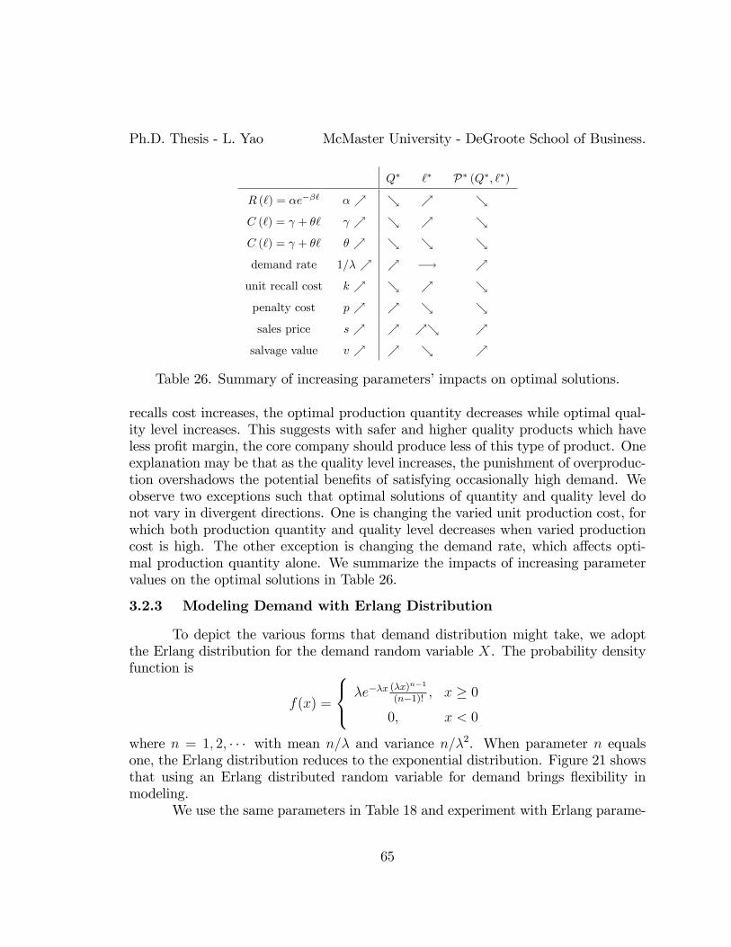
Ph.D. Thesis - L. Yao McMaster University - DeGroote School of Business.
Q∗ `∗ P∗ (Q∗, `∗)
R (`) = αe−β` α
C (`) = γ + θ` γ
C (`) = γ + θ` θ
demand rate 1/λ −→
unit recall cost k
penalty cost p
sales price s
salvage value v
Table 26. Summary of increasing parameters’impacts on optimal solutions.
recalls cost increases, the optimal production quantity decreases while optimal qual-ity level increases. This suggests with safer and higher quality products which haveless profit margin, the core company should produce less of this type of product. Oneexplanation may be that as the quality level increases, the punishment of overproduc-tion overshadows the potential benefits of satisfying occasionally high demand. Weobserve two exceptions such that optimal solutions of quantity and quality level donot vary in divergent directions. One is changing the varied unit production cost, forwhich both production quantity and quality level decreases when varied productioncost is high. The other exception is changing the demand rate, which affects opti-mal production quantity alone. We summarize the impacts of increasing parametervalues on the optimal solutions in Table 26.
3.2.3 Modeling Demand with Erlang Distribution
To depict the various forms that demand distribution might take, we adoptthe Erlang distribution for the demand random variable X. The probability densityfunction is
f(x) =
λe−λx (λx)n−1
(n−1)! , x ≥ 0
0, x < 0
where n = 1, 2, · · · with mean n/λ and variance n/λ2. When parameter n equalsone, the Erlang distribution reduces to the exponential distribution. Figure 21 showsthat using an Erlang distributed random variable for demand brings flexibility inmodeling.
We use the same parameters in Table 18 and experiment with Erlang parame-
65

Ph.D. Thesis - L. Yao McMaster University - DeGroote School of Business.
Figure 21. Erlang distributed demand X with n = 1, 2, 3 and λ = 0.01.
66

Ph.D. Thesis - L. Yao McMaster University - DeGroote School of Business.
ter n increasing from 1 to 5. Table 27 shows the numerical results that both optimalordering quantity Q∗ and quality level `∗ increases as n increases. Our parametricanalysis in Section 3.2.2 exemplifies that increasing average demand rate 1/λ in ex-ponential distribution leads to higher optimal ordering quantity but has no impact onoptimal quality level. Increasing Erlang parameter n also results in a larger averagedemand rate n/λ and increases both Q∗ and `∗ concurrently. This difference may beattributed to the influence of n on the shape of Erlang distribution – when n grows,the probability density function curve is pressed down and shifted to the right withless skewness.
n P∗ (Q∗, `∗) Q∗ `∗
1 311 130 2.55
2 1102 254 2.69
3 1992 373 2.76
4 2931 488 2.80
5 3899 601 2.83
Table 27. With Erlang distributed demand, both optimal ordering quantity andquality level increases when Erlang parameter n increases.
When applying first order optimality condition to the objective P (Q, `), weobserve increasing Erlang parameter n has more notable impacts on the partial dif-ferential function ∂P (Q, `) /∂Q. Figure 22 shows that increasing Erlang parametern does not significantly impact the shape of two implicit differential function curvescomparing to using exponential distribution, but pushes the curves up and to theright, which explains the increase of both ordering quantity and quality level in opti-mal solution.
3.3 Extending the Model with External Suppliers
In practice, companies do not always own the manufacturing of its productsor viewing production as its core competence. For instance, a typical warehouseretailer does not produce any of the products on its shelves; instead, it depends onmultiple suppliers for high quality products supply. Therefore, we want to examine theimpacts of using multiple external suppliers as the production sources. In this case,the product quality level is no longer within the direct control of the core company(the seller). However, the company can indirectly control the product quality levelby offering suppliers higher purchase price on meeting higher quality standards.
67

Ph.D. Thesis - L. Yao McMaster University - DeGroote School of Business.
Figure 22. Implicit plots using first order optimality conditions shows increasingErlang parameter n does not change the shape of two function curves significantlybut pushes the curves up and to the right, which explains the increasements of bothdecision variables in optimal solution.
68

Ph.D. Thesis - L. Yao McMaster University - DeGroote School of Business.
Supplier S1 S2
Product quality level `1 `2
Unit production cost c1 (`1) c2 (`2)
Recall probability R1 (`1) R2 (`2)
Order quantity Q1 Q2
Demand random variable X1 ∼ f1 (x1) X2 ∼ f2 (x2)
Table 28. Variables and functions for the extension of two suppliers.
Here is a real life example from our neighborhood. Fortinos is a chained re-tailer owned by Loblaw which offers daily grocery for its customers. Loblaw sellsproducts of its own brand Presidential Choice (PC) on a variety of convenient veg-etable packages, organic produce, processed foods (cakes and ice cream) and etc. Ofa common produce, spinach, Fortinos offers two types of products from two separatesuppliers. One is the cooking spinach which costs $2.55 per 500 grams; the otheris the organic baby spinach which costs $5.99 per 500 grams. The organic spinachwould have higher quality standards on freshness, appearance and bacteria controlalong with other production requirement of being organic. While including two ormore suppliers in its supply chain, Fortinos would seek the best ordering quantitiesand quality standards when managing its suppliers to optimize its expected profit.
3.3.1 Modeling with Two Suppliers
Suppose the seller collaborates with two suppliers (S1 and S2) that specializein manufacturing. We use random variable X1 with PDF f1 (x1) to denote demandsatisfied by S1, random variable X2 with PDF f2 (x2) for demand satisfied by S2, andX1 and X2 are independent. Suppose the seller is aware of the cost-quality relationsof both suppliers from historical data. Based on the seller’s required quality level,unit manufacturing cost from suppliers (i = 1, 2) follows the function ci (`i) where `iis the required product quality level. The seller also determines purchase quality ofeach supplier (Qi) to maximize his expected total profits considering the risks of apotential product recall. The product recall probability of suppliers (i = 1, 2) followsthe function Ri (`i) . Table 28 shows variables and functions for the two suppliers.
The focus of this proposed study is to examine impacts of the cost functionsand recall probability functions on the seller’s optimal order quantities, product qual-ity levels, and the expected profits. There are four cases of possible recall situations,for which we use ‘0’to denote recall and ‘1’to denote good products with no recalland represent the four cases in Table 29.
Four events happen in the single period of decision making, including ordering
69

Ph.D. Thesis - L. Yao McMaster University - DeGroote School of Business.
Supplier S1 S2 Probability Profit function
Both are good 1 1 (1−R1 (`1)) (1−R2 (`2)) Π11
Only S2 recalls 1 0 (1−R1 (`1))R2 (`2) Π10
Only S1 recalls 0 1 R1 (`1) (1−R2 (`2)) Π01
Both recall 0 0 R1 (`1)R2 (`2) Π00
Table 29. Four cases of suppliers recall situations.
70

Ph.D. Thesis - L. Yao McMaster University - DeGroote School of Business.
Begin End
Order Q Demand Recall(Possibly, R(l))
ProductionCost c(l)
Sale RecallCost
Salvage/Penalty
Figure 23. Four events in single period decision-making process.
products with quantity Qi and quality level `i from supplier i (i = 1, 2), satisfyingdemand (X1 = x1 and X2 = x2) and obtain sale income, incurring recall costs ifrecall happens, or incurring penalty costs and collecting salvage values if recall doesnot happen. Figure 23 illustrates the sequence and outcome of the above four events.
Hence, the total expected profit (E (Π)) of one-stage stochastic newsvendorquality control model with two suppliers is
E (Π) =1∑i=0
1∑j=0
E (Πij | S1 = i, S2 = j) Pr (S1 = i, S2 = j) (33)
where
Π11 = s [min (X1, Q1) + min (X2, Q2)]− [c1 (`1)Q1 + c2 (`2)Q2]
+v [(Q1 −min (X1, Q1)) + (Q2 −min (X2, Q2))]
−p [(X1 −min (X1, Q1)) + (X2 −min (X2, Q2))]
Π10 = s [min (X1, Q1) + min (X2, Q2)]− [c1 (`1)Q1 + c2 (`2)Q2]
+v [Q1 −min (X1, Q1)]− p [X1 −min (X1, Q1)]− kmin (X2, Q2)
Π01 = s [min (X1, Q1) + min (X2, Q2)]− [c1 (`1)Q1 + c2 (`2)Q2]
+v [Q2 −min (x2, Q2)]− p [X2 −min (X2, Q2)]− kmin (X1, Q1)
Π00 = s [min (X1, Q1) + min (X2, Q2)]− [c1 (`1)Q1 + c2 (`2)Q2]
−k [min (X1, Q1) + min (X2, Q2)]
and probabilities Pr (S1 = i, S2 = j) are shown in Table 29. This model may be ex-tended for multiple suppliers by adding the set of decision variables (Qi, `i) and func-tions (ci (`i) , Ri (`i)) for each supplier i (i = 1, 2, . . . , n). We will explore the solutionmethods and discover insights for the proposed model of two or more suppliers.
71

Ph.D. Thesis - L. Yao McMaster University - DeGroote School of Business.
3.3.2 Numerical Studies
We explore the impacts to the optimal solution of four cases: (1) the secondsupplier takes additional demand; (2) the two suppliers share demand evenly; (3)demand-sharing while decreasing production cost of the second supplier; (4) demand-sharing and two suppliers have different prices. Supplier One’s parameters are thesame as in base case for internal supply (Section 3.2.1).
3.3.2.1 Case 1. S2 takes additional demand.
α1 β1 γ1 θ1 λ1 α2 β2 γ2 θ2 λ2 k p s v
0.9 1 5 2 1/100 0.96 1 6 2.5 1/50 50 6 25 4
Q∗1 `∗1 Q∗2 `∗2 P∗ (Q∗1, `∗1, Q
∗2, `∗2)
129.69 2.55 49.26 2.47 330.28
Table 30. Parameter setting and optimal solutions for case 1 the second supplier takesadditional demand.
The results suggest adding the second supplier does not affect the optimalsolution of supplier one (S1) even that S1 may serve customers of S2 in case thatS2 initiates a recall. This might attribute to the small probability setting of bothsuppliers, especially of the newly added supplier S2.
3.3.2.2 Case 2. S1 and S2 share the demand evenly.
When both suppliers now share the original setting of 100 demand evenly, theresults show each supplier optimize its process separately as if they are supplyingalone with the half demand. Reducing demand alone does not impact the optimalquality level, but reduces the optimal order quantity the same way demand alters,which is consistent with our numerical findings of internal supply case. We noticethat supplier two (S2) has slightly lower quality level but much less order quantity inoptimal solutions comparing to supplier one, the reason is its high production cost.Thus in case 3 we aim to examine the effects of improving production cost.
3.3.2.3 Case 3. Demand-sharing while decreasing production cost of S2.
By improving production cost of supplier two, the solutions show that bothits quality level and ordering quality improve, which echo with results in our previousnumerical analysis in Section 3.2.1.
3.3.2.4 Case 4. Demand-sharing and two suppliers have different prices.
72

Ph.D. Thesis - L. Yao McMaster University - DeGroote School of Business.
α1 β1 γ1 θ1 λ1 α2 β2 γ2 θ2 λ2 k p s v
0.9 1 5 2 1/50 0.96 1 6 2.5 1/50 50 6 25 4
Q∗1 `∗1 Q∗2 `∗2 P∗ (Q∗1, `∗1, Q
∗2, `∗2)
64.84 2.55 49.26 2.47 170.80
Table 31. Parameter setting and optimal solutions for case 2 demand-sharing evenlybetween two suppliers.
α1 β1 γ1 θ1 λ1 α2 β2 γ2 θ2 λ2 k p s v
0.9 1 5 2 1/50 0.96 1 4 1.5 1/50 50 6 25 4
Q∗1 `∗1 Q∗2 `∗2 P∗ (Q∗1, `∗1, Q
∗2, `∗2)
64.84 2.55 84.41 2.79 475.49
Table 32. Parameter setting and optimal solutions for case 3 demand-sharing andcost-improved second supplier.
α1 β1 γ1 θ1 λ1 α2 β2 γ2 θ2 λ2 k p s1 s2 v
0.9 1 5 2 1/50 0.96 1 4 1.5 1/50 50 6 30 20 4
Q∗1 `∗1 Q∗2 `∗2 P∗ (Q∗1, `∗1, Q
∗2, `∗2)
74.93 2.50 72.26 2.86 465.86
Table 33. Parameter setting and optimal solutions for case 4 demand-sharing anddifferent prices.
73

Ph.D. Thesis - L. Yao McMaster University - DeGroote School of Business.
Figure 24. Expected profit (E (Π)) is concave on ordering quantities when fixingoptimal quality levels `∗1 and `
∗2.
Case 4 is modified based on case 3 that both suppliers share the demand evenlybut in this case supplier S1 has higher price ($30) and supplier S2 has lower price($20) compared to the unified price $25 in case 3. With increased price, the optimalordering quantity increases by 10.09 for S1 but the quality level decreases by 0.05.Similarly for S2 as the price decreases the optimal ordering quantity decreases by12.15 and the quality level increases by 0.07. These results are consistent with ouranalysis of price changes for internal supply in Section 3.2.1.
One surprising result shown in case 4 is that the more expensive products ofS1 have lower optimal quality level than the less expensive products of S2 comparingtheir cost structure. This counter intuitive result suggests a high cost and high sellingprice product could have lower optimal quality level because higher profit margin doesnot incent quality improvement. On the contrary it may accommodate the recall risksand allow lower quality.
3.3.3 Concavity Results
We explore the concavity of the proposed model (33) by isolating the order-ing quantities/quality levels while setting the remaining decision variables with theiroptimal solution values. The results show the expected profit function is concaveon both ordering quantities and quality levels as shown in Figure 24 and Figure 25respectively.
74
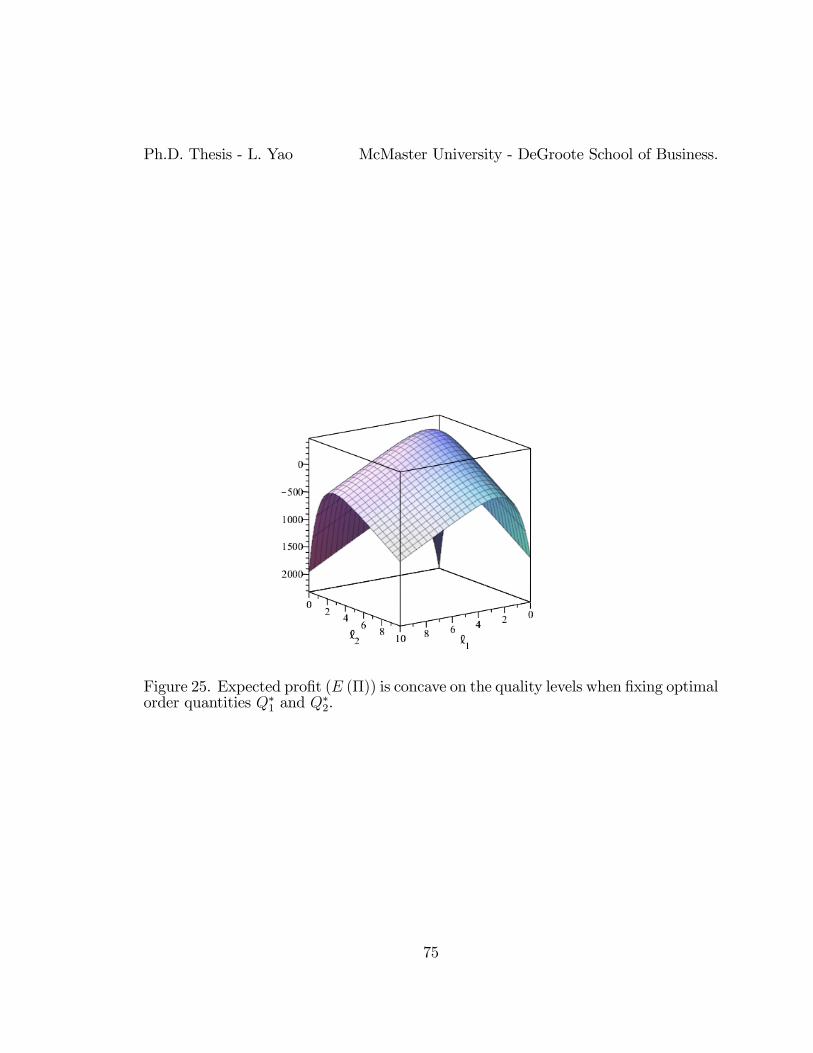
Ph.D. Thesis - L. Yao McMaster University - DeGroote School of Business.
Figure 25. Expected profit (E (Π)) is concave on the quality levels when fixing optimalorder quantities Q∗1 and Q
∗2.
75

Ph.D. Thesis - L. Yao McMaster University - DeGroote School of Business.
3.4 Conclusion
In this chapter we extend the newsvendor problem for product recall riskmanagement by optimizing both quality level and ordering quantity. Our main con-tribution is that we model and solve the optimization problem of product recall man-agement by incorporating quality control in the classic newsvendor problem. We addquality-dependent functions for recall probability and production cost so that recallrisks can be well quantified in the objective function.
Our first discussion centers on the internal supply case in which the core com-pany has direct control of quality level. Concavity analysis shows the objective isneither concave nor convex in the feasible region, but applying the first and secondorder optimality conditions can effectively find the optimal solution. Our numericalanalysis shows in most cases an inverse relationship between optimal ordering quan-tity and quality level as summarized in Table 26. One counter-intuitive finding isthat higher selling price does not incentivize investment on quality levels, insteadit promotes lower quality level since higher profit margin can accommodate higherpotential costs of recall.
We extend our model to external multiple suppliers, especially the case of twosuppliers. Both suppliers satisfy their own demands independently and supply foreach other’s customers only when the other party has a recall. Our results showthat the prospect of covering the other party’s demand in case of recall has verylittle impact on either supplier’s optimal ordering quantity and quality level. In otherwords, the optimal solutions are determined by parameter and function settings ofthe individual supplier. Our concavity analysis suggests that the objective is concavefor quality levels (ordering quantities) of the two suppliers when ordering quantities(quality levels) are set to be optimal.
76

Ph.D. Thesis - L. Yao McMaster University - DeGroote School of Business.
Chapter 4Optimal Facility Location to MitigateProduct Recall Risks
This chapter is motivated by major food product recall events in recent years,especially how the timely and effective response using post-recall management canmake a difference. We consider the rare but very influential major product recallsas disruptions to the supply chain and incorporate locating reprocessing centers forthe returned products to mitigate expected operational costs. We adopt the closedloop network design framework and assume the location decisions for reprocessingcenter take place after the product recall events. Our scenario based analysis showsthe approach is effective in both absolute and relative measures.
4.1 Introduction
In September 2012, the rejection of ground beef imports by the U.S. customand the later outbreak of the E.coli disease forced XL Inc. (XL) to start a series ofbeef recalls, which turned out to be the largest meat recall event in Canada history.The recall of 1,800 products impacted over 33 retail chains across Canada. Over4,000 tons of meat and meat products were sent back to plants for disposal. Thisunprecedented amount of recalled products overwhelmed the capacities of any existingdisposal methods of XL, the largest domestically owned meat processor in Canadaat the time, resulting in 600 tons of frozen beef being sent directly to landfill. Thefailure to adequately process recalled products raised the public concern over XL’scapability to maintain food safety. This incident eventually led to a transfer of XL’sownership for the Calgary plant. Charlebois et al. [9] discussed this event and itsimpacts in detail.
In comparison, when facing the 2008 Listeria outbreak, Maple Leaf Food Inc.(MLF) recalled all potentially affected products promptly and dealt with the disposalof 1,300 tons of beef and beef products. MLF’s actions bought time to discover thecontamination source and recover the brand. Nevertheless, there was a substantialdirect cost of $19 million related to recall activities (e.g., collection and destruction,shutdown and sanitation of facility, media, and customer response call center). Intotal, MLF suffered approximately $200 millions loss in this incident.
Food safety is generally referred to as the prevention of illness resulting fromthe consumption of contaminated food as discussed by Akkerman [1]. This topic
77

Ph.D. Thesis - L. Yao McMaster University - DeGroote School of Business.
has attracted more attention recently because of the growing rigorous governmentstandards as well as the large social and financial impacts of major food safety fail-ure. Effective control of food safety along the supply chain is important but verycomplicated because food is vulnerable to contamination and food supply chains aresophisticated. For example, Desmarchelier et al. [15] provide a summary of foodsafety management in the red meat industry of Australia. Risk mitigation strategiesare applied in the entire food supply chain.
However, food borne disease is a critical inherent risk factor in food manufac-turing and distribution, due to the indigenous existence of microbial contaminationsin raw food materials, natural growth of pathogens, inevitable mistakes in manualoperations, contamination and other factors. In response to food safety incidents,business and society adopt food recalls to correct the situation and mitigate mon-etary and social costs. Manufacturing companies manage food recalls by collectingproducts from their distribution channels and adopting best methods to reconditionand dispose recalled products.
Proper preparation could help companies manage food recalls more effi cientlyand effectively, especially in strategic planning. For example, firms could use location-allocation decisions for both manufacturing plants and reprocessing facilities for re-called products. Linking to optimization studies, Akkerman et al. [1] provide a reviewof improving food supply chain management with network planning models. Foodquality, food safety and sustainability are considered as key objectives. Three lev-els of network planning models are considered, namely strategic network design (e.g.,facility location-allocations), tactical network planning (e.g., production and distri-bution) and operational transportation planning (e.g., routing). They suggest thatstrategic network design is critical in food safety control, impacting how long foodproducts travel and how widely the products spread geographically, both of whichdetermine the size of potential product recalls.
This chapter addresses the supply chain safety control issue by designing thesupply chain network to incorporate the negative effects of product recalls. Althoughour model is motivated by food recall, it can be applied to any supply chain withsignificant impacts of recall events. Extending from the closed-loop network designconcept, this work focuses on managing the reverse flow (recalled products) in a cost-effi cient manner. However, rather than maintaining a closed-loop supply chain on adaily basis as in most studies (e.g., repair and post-sale service systems), we studythe effi cient way of managing random and rare major product recalls. The features ofrareness and randomness of major products recalls lead us to disruption managementstudies in which researchers focus on how to consistently satisfy customer demandsgiven that some suppliers may fail. Our focus is different in that we consider how toquickly build a reprocessing network to dispose recalled products.
78

Ph.D. Thesis - L. Yao McMaster University - DeGroote School of Business.
We study the location-allocation problem with random occurrence of productrecalls and treat the recall incidences as disruptions to the supply chain. In our set-ting, the company first makes decisions to locate manufacturing plants and allocatedemands. After the product recall occurs, we make decisions to locate the reprocess-ing center(s) from internal (self-owned recall facility) or external (third-party busi-ness) sources and allocate recalled products for reprocessing or local disposal. Threefeatures distinguish our problem from other location-allocation problems. Firstly, fa-cility location and allocation decisions occur in two stages. Secondly, the second stagelocation-allocation happens under uncertainty. Thirdly, reverse logistic flows exist inthe second stage.
We design a two-stage stochastic mixed integer programming model, in whichwe locate the manufacturing plants in the first stage and the reprocessing/disposalfacilities in the second stage. We adopt a scenario-based approach to describe theuncertainty of major recall events that may happen in manufacturing plants as well asof availability of reprocessing facilities. Given the complexity induced by our nestedfacility location problem, we devise an algorithm based on Lagrangian relaxation tosolve the uncapacitated case.
This chapter will be organized as follows. Section 4.2 provides a brief reviewof literature. Section 4.3 introduces the mathematical model, an analysis based onfacility capacities, and a Branch-and-Bound algorithm incorporating Lagrangian re-laxation for the uncapacitated case. Section 4.5 presents the computational resultsand managerial insights from experiments. Section 4.6 summarizes contributions anddiscusses further research directions.
4.2 Literature Review
There are two research streams closely related to our research, i.e., reliable sup-ply chain network design, and location-allocation with bidirectional logistical flows.
There is a well-developed literature on modeling supply chain disruption man-agement. Snyder et al. [48] provide a review of optimization models in supply chainnetwork planning with disruption management. They categorize by network status,underlying mathematical models and risk measures. They show various models ex-tending the classical P-median and Uncapacitated Facility Location Problem (UFLP),Capacitated Facility Location Problem (CFLP) models with reliability features (i.e.,consistent satisfaction of demands when some facilities fail in random disruptions).Qi et al. [37] consider a fortification model with disruptions. They manage locations,allocations and inventory. Both suppliers and retailers can experience random dis-ruptions. Qi et al. [36] examine different sourcing and replenishment decisions withtwo suppliers. Dada et al. [11] develop a newsvendor procurement model selecting
79

Ph.D. Thesis - L. Yao McMaster University - DeGroote School of Business.
from multiple unreliable suppliers. Their results suggest that newsvendor, customersand retailers perceive different service level changes when disruption occurs. Com-pared to reliability concerns, cost is the most determinant factor. This body of workfocuses on satisfying customer demand —there is no focus on reverse flow.
On the other hand, in closed-loop supply chain models, the emphasis is tominimize the long-run average cost of forward and reverse flows, which does notmodel the random occurrence of product recalls. Uncertainty in closed-loop supplychain network design is not always considered. Some studies use a fixed return ratebased on historical data (e.g., Min and Ko [31], Salema et al. [41], Lu and Bostel[25], and Lee and Dong [22]). Savaskan et al. [45] describe product return rate as afunction of investment used to promote product return.
Hitherto, uncertain factors in closed-loop supply chain include return rate,demand for re-manufactured products (secondary market), quality of returned prod-ucts, and variable costs for collection, processing and transportation. Pishvaee et al.[34] describe uncertain demands, returns and transportation costs given by a robustnetwork design model. Salema et al. [42] address uncertain demand and return withscenario dependent uniform random numbers to minimize the total cost of the reverselogistics network. Ramezani et al. [38] consider uncertainty in demand and return ra-tio as well as various variable costs in their multi-objective forward/reverse networkdesign. Listes [24] uses scenario-dependent parameters to describe uncertain demandand returned product quantity for their supply and product-return networks. Few re-searchers assume the scenario of randomly failing manufacturing plants which resultsin major recall events.
The literature has taken different approaches to deciding the quantity to dis-pose during returned products collection and reprocessing. Early literature tends tonot consider disposal cost. For instance, Savaskan et al. [45] do not take disposal asa cost factor when comparing different re-manufacturing channels. With increasingfocus on environment-friendly and effi cient supply chains, disposal costs are reflectedin later studies. For example, Min and Ko [31] alter the repair facility capacities toaccommodate returned quantities at each time period so no disposal will occur.
Decisions regarding disposal cost can be categorized in three types: fixed ra-tios, market driven and cost driven. Fixed disposal ratios are deduced from historicaldata and adopted to simplify the model (e.g., Pishvaee et al. [34], Lu and Bostel [25],and Lee and Dong [22]). Cost driven decisions aim to minimize total cost of collec-tion, reprocessing and disposal. Salema et al. [42] minimize total supply chain costsby using fraction of customer demand used for disposal or recovery. Ramezani et al.[38] use disposed quantity to maximize the total profit within the capacity of openeddisposal centers. Market driven decisions select the best efforts to satisfy demands ofsecondary market. Pishvaee et al. [34] model the disposal quantity as decision vari-
80

Ph.D. Thesis - L. Yao McMaster University - DeGroote School of Business.
able so that secondary market can be satisfied in the most effi cient way. Listes [24]take the perspective that returned products can be disposed in two decisions: beforecollection and before reprocessing, both of which aim to maximize the total profitwhile satisfying market demands.
In summary, the existing literature treats reverse flow on day-to-day basis.This modeling approach does not serve major product recalls well. Our challenge isto design an optimal network that can accommodate product returns in the contextof major product recalls.
4.3 Facility Location to Mitigate Recall Risks
4.3.1 Model Development
In this section, we use a two-stage stochastic programming approach describedby Ruszczynski and Shapiro [40] to model the problem. In the first stage, we makefacility location and transportation decisions. In the second stage, under each disrup-tion scenario, we make recall decisions including recall facility locations (e.g., centersfor reconditioning, reprocessing, and rendering) and recall allocation decisions (e.g.,use local disposal or recall center). The objective is to minimize the sum of facilitylocation costs, transportation costs and recall costs.
Define I as the set of candidate locations for manufacturing facilities, and usei as the index. Define K as the set of candidate locations for recall centers and usek as the index. Note that recall centers could reuse the manufacturing facilities, oruse third party processing facilities. Thus we could have I ⊂ K or I
⋂K = ∅. We
use FF and RF to indicate forward product flow and reverse product flow (initiatedby recall events) respectively. Clearly, facilities built for manufacturing and recallprocessing have different fixed costs, defined as fFFi and fRFk . Facility capacity isdenoted by MFF
i or MRFk .
Define J as the set of retailers and use j as the index. Each retailer has ademand Dj, the cost of shipping one unit of product demand from facility i to retailerj is cFFij , while the reverse flow costs c
RFjk per unit. For recalled products, two recall
modes are available, i.e., local disposal and central processing. Local disposal incurs aretailer location related cost cLDj , and central processing incurs a recall center relatedcost cCPi .
To describe the uncertainty of facility disruption, we use scenario set S andindex s. We used ps to denote the probability of scenario s. Manufacturing facilitiesfailing in scenario s is denoted by set Is. Accordingly, recall centers available inscenario s is denoted by set Ks. The choice of Ks can be decided extraneously.
81
Ph.D. Thesis - L. Yao McMaster University - DeGroote School of Business.
For instance, recalled products could be prohibited from returning to their originalmanufacturing facility due to safety concerns, or be sent to third party facilities dueto economic considerations.
Decision variables used in this model are facility location variables (X formanufacturing facilities and Z for recall facilities), transportation variables (Y ), andrecall assignment variables (V for local disposal andW for central processing):
Xi =
1 manufacturing facility at location i is open0 otherwise.
Zks =
1 recall facility is open at location k under scenario s0 otherwise.
Yij : quantity transported from facility i to retailer jVjs : quantity for local disposal under scenario s at retailer jWjks : quantity from retailer j to plant k for central processing under s
With these notations, the two-stage stochastic program for the Facility Location withRecall Problem (FLRP) is formulated as follows:
82

Ph.D. Thesis - L. Yao McMaster University - DeGroote School of Business.
(FLRP) min∑i∈I
fFFi Xi +∑i∈I
∑j∈J
cFFij Yij
+∑s∈S
ps
[∑k∈Ks
fRFk Zks +∑k∈Ks
∑j∈J
(cRFjk + cCPk
)Wjks +
∑j∈J
cLDj Vjs
](34)
s.t.∑i∈I
Yij = Dj ∀j ∈ J (35)∑j∈J
Yij ≤MFFi Xi ∀i ∈ I (36)∑
j∈JWjks ≤MRF
k Zks ∀s ∈ S, k ∈ Ks (37)∑k∈Ks
Wjks + Vjs =∑i∈Is
Yij ∀j ∈ J , s ∈ S (38)
Yij ≥ 0 ∀i ∈ I, j ∈ J (39)Wjks, Vjs ≥ 0 ∀j ∈ J, s ∈ S, k ∈ Ks (40)Xi ∈ 0, 1 ∀i ∈ I (41)Zks ∈ 0, 1 ∀s ∈ S, k ∈ Ks (42)
The objective (34) is the expected total cost of facility location-allocationdecisions from both stages. In the first stage, the manufacturing facility locationand demand distribution are determined, while in second stage, recall center locationand recall product distribution are determined. Constraint (35) ensures demand ofeach retailer is satisfied. Constraint (36) and (37) guarantees forward and recalledproducts are processed in an open facility within the capacities. Constraint (38)requires recalled products either be sent back to recall center for reprocessing ordisposed locally. Other constraints are for non-negativity and for binary variables.
It is noteworthy that the proposed formulation is very general and can includedifferent recall situations. Firstly, the model can cover cases of capacitated anduncapacitated facilities or any hybrid types by changing the capacity parameterMFF
i
and MRFk to be infinite or finite numbers. Secondly, the definition of set Ks provides
a lot of flexibility in modeling. For instance, facilities in Ks can be the exact locationswhere the food safety incidents happen, suggesting that recalled products must returnto their original manufacturing plants; a type of corrective action in this situation isto fix problems such as mislabeling. We can also require facilities in Ks be locationsother than the original manufacturing facilities to model the situation in which theoriginal facilities are unsuitable for processing (e.g., safety overhaul). Moreover, Ks
83

Ph.D. Thesis - L. Yao McMaster University - DeGroote School of Business.
could be third party facility locations to model the outsourcing of processing recalledproducts. Thirdly, for further extension, recall facility location decisions Zks’s couldbe moved to the first stage. The difference between this extension and (FLRP) willshow the difference between prepared recall facility location decisions and reactivefacility location decisions.
In addition, the model could indicate different traceability capability in for-ward flow. Currently, we assume full traceability in forward flow, i.e., each retailercould distinguish the products from failed plants from others. We can also modelincomplete traceability such that retailer can’t identify the source of the recalledproducts, by altering constraint (38) to
∑k∈KsWjks + Vjs =
∑i∈I Yij for all j ∈ J
and s ∈ S.
4.3.2 Analysis
If the demand of a retailer is satisfied by more than one facility, it is called “de-mand splitting”, otherwise, it is called “no demand splitting”. Note that (FLRP)contains two types of demands, corresponding to the two stages (i.e., customer de-mand and recall demand). To be concise, we use “plants”to denote manufacturingcenters located for forward flows, and “facilities” to denote processing centers lo-cated for reverse flows. We have the following result in the optimal demand splittingschemes of (FLRP):
Theorem 7 In the optimal solutions of (FLRP), demand splitting schemes of for-ward and reverse flows depend on the capacity constraints of both plants and facilities.There are four schemes:
(a)If plants and facilities are both uncapacitated, then there exists no demand split-ting for both forward and reverse flows;
(b)If plants are capacitated but facilities are uncapacitated, then there exists demandsplitting for forward flow and no demand splitting for reverse flow;
(c)If plants are uncapacitated but facilities are capacitated, then there could existdemand splitting for both flows;
(d)If plants and facilities are both capacitated, then there could exist demand split-ting for both flows.
Proof. Consider an arbitrary retailer u ∈ J . Assume that except the allocationdecisions for u, all other decisions are fixed to their optimal values. We use superscript∗ to represent the optimal values. These decisions include:
X∗i (i ∈ I) locating plants for forward flow,Z∗ks(k ∈ Ks, s ∈ S) locating facilities for reverse flow,
84

Ph.D. Thesis - L. Yao McMaster University - DeGroote School of Business.
Y ∗ij(i ∈ I, j ∈ J \u) allocating demands of retailers other than u in forwardflow,
V ∗js,W∗jks (j ∈ J \u, k ∈ Ks, s ∈ S) allocating recall demands of retailers other
than u for central reprocessing and local disposal respectively in reverse flow.In the following, we discuss the demand splitting schemes in two steps. We
isolate demand splitting decisions in the reverse flow in the first step, and apply theresults in the second step to integrate both forward and revers flows. Note we use ∗to denote optimal solutions for (FLRP) in this proof, while later in algorithm designwe use ∗ to denote best solutions found in Lagrangian relaxation.
Step 1. Demand allocations in forward flows, i.e., Y ∗iu (i ∈ I), are known andoptimal.
We use K∗s to denote the set of facilities to open for reverse flow in scenarios ∈ S in the optimal solution. Let βks be the proportion of demand for retailer uallocated to facility k ∈ K∗s in scenario s, β′s be the proportion of demand allocatedto local disposal in scenario s. We have
∑k∈K∗s βks + β′s = 1 in scenario s.
Let D∗us be the optimal recall demand from u in scenario s. Note that whenforward flow is traceable, we have D∗us =
∑i∈Is Y
∗iu; when forward flow is untraceable,
we have D∗us =∑
i∈I Y∗iu if Y
∗iu > 0 for some i ∈ Is, and D∗us = 0 otherwise.
Using Ω to denote the total cost of known location and allocation decisions,(FLRP) can be simplified as follows:
min Ω +∑s∈S
ps
[ ∑k∈K∗s
(cRFuk + cCPk
)βksDus + cLDu β′sDus
]s.t.
∑k∈K∗s
βks + β′s = 1∀s ∈ S
βksDus +∑
j∈J\uW ∗jks ≤MRF
k ∀k ∈ K∗s , s ∈ S
βks, β′s ≥ 0 ∀k ∈ K∗s , s ∈ S.
Note that local disposal at retailer u always has unlimited capacity. This setting canbe altered by adding constraint β′sDus ≤ MRF
u in the analysis, where MRFu is the
capacity for local disposal of u.If the facilities are uncapacitated, the optimal solution is either 0 or 1 because
the objective function is a linear function of βks and β′s defined on interval [0, 1]. In
other words, there is no demand splitting for any scenario s ∈ S. Denote
γ∗s = min
cLDu , min
k∈K∗s
cRFuk + cCPk
,
and optimal recall cost of u as ψ∗s(D∗us) = γ∗sD
∗us, then the optimal objective value is
85

Ph.D. Thesis - L. Yao McMaster University - DeGroote School of Business.
Ω +∑
s∈S psψ∗s(D
∗us).
If the facilities are capacitated, in order to minimize the objective function,we sort the coeffi cients (cRFuk + cCPk ) (k ∈ K∗s) and cLDu in increasing order, denotedas c1, c2, · · · , cns+1 where ns = |K∗s|. Then the optimal solution is to assign demandaccording to this order given the capacity constraints. We redefine reverse flow costψ∗s(D
∗us) as follows:
ψ∗s(D∗us) =
c1D
∗us D∗us ≤MRF
1
ck+1
(D∗us −
k∑i=1
MRFi
)+
k∑i=1
ciMRFi
k∑i=1
MRFi ≤ D∗us ≤
k+1∑i=1
MRFi
∀k = 1, · · · , ns
where c1 ≤ c2 ≤ · · · ≤ cns ≤ cns+1. Note that if the unit cost of local disposal isranked before that of facility j, then calculations for facility j and its followers areunnecessary because local disposal is uncapacitated.
We have the same form of optimal objective value Ω +∑
s∈S psψ∗s(D
∗us). Note
that reverse flow cost ψ∗s(D∗us) is a continuous and nondecreasing piece-wise linear
function ofD∗us when facility capacities are limited. Clearly ψ∗s(·) is a convex function.
Step 2. In the optimal solution, denote I∗ as the set of plants open in forwardflow, I∗s as the set of plants that are open and get disrupted in scenario s ∈ S. Let αibe the proportion of demand allocated to plant i ∈ I∗ for forward flows, ψ∗s(D∗us) bethe optimal cost for reverse flow as defined in Step 1, where D∗us =
∑i∈I∗s αiDu (or in
the case with untraceable demand, if Y ∗iu > 0 for some i ∈ I∗s , then D∗us = Du). LetΨ be the cost of all known optimal decisions. (FLRP) can be simplified as follows:
min Ψ +∑i∈I∗
cFFiu αiDu +∑s∈S
psψ∗s
∑i∈I∗s
(αiDu)
s.t.∑i∈I∗
αi = 1
αiDu +∑
j∈J\uY ∗ij ≤MFF
i ∀i ∈ I∗
αi ≥ 0 ∀i ∈ I∗
If facilities are uncapacitated, then ψ∗s(D∗us) = γ∗sD
∗us = γ∗s
∑i∈I∗s αiDu. Clearly,
the objective function is linear in αi’s. It holds that when plants are uncapacitated,the plant incurring the lowest cost will be chosen, thus the optimal solution doesnot have demand splitting for neither forward nor reverse flows, which completes theproof for Theorem 7 Scheme (7). On the other hand, with capacitated plants the op-timal demand splitting scheme for reverse flow remains to be no demand splitting;while capacity limits of plants in forward flow require demand splitting to satisfy all
86
Ph.D. Thesis - L. Yao McMaster University - DeGroote School of Business.
demands at the lowest cost, which completes the proof for Theorem 7 Scheme (7).In the case of capacitated facilities and uncapacitated plants, apparently de-
mand splitting in reverse flow exists because of facility capacity limits, would thedemand splitting in reverse flow lead to demand splitting in forward flow even whenthere is no restriction on plant capacity?
Suppose, on the contrary, there is no demand splitting in the optimal decision.Consider the retailer u has demand Du, served by two plants I∗ = i1, i2 and twofacilities K∗s = k1, k2 that are open for all scenarios. Plants fail independently. Letus compare the following two cases.
In the first case, Du is completely served by plant i1 ∈ I∗. Denote the proba-bility of failure of i1 as qi1 =
∑s:i1∈I∗s ps, called the failure rate of i1. The allocation
cost TC1 for i1 can be represented as TC1 = cFFi1uDu + qi1ψ(Du). Note we use ψ(·) in-stead of ψ∗(·) because it is not optimal solution. In the second case, Du is satisfiedby two plants i1 and i2. Let αi1 and αi2 denote the proportions of demand Du sat-isfied by i1 and i2 respectively, where αi1 + αi2 = 1. Let the failure rates of plantsi1 and i2 be qi1 and qi2 respectively. Then the total allocation cost TC2 would beTC2 = αi1c
FFi1uDu+αi2c
FFi2uDu+qi1(1−qi2)ψ(αi1Du)+(1−qi1)qi2ψ(αi2Du)+qi1qi2ψ(Du)
. Comparing TC1 and TC2:
TC1 − TC2 =(1− αi1)cFFi1uDu − αi2cFFi2uDu − qi1(1− qi2)ψ(αi1Du)
− (1− qi1)qi2ψ(αi2Du) + qi1(1− qi2)ψ(Du)
=αi2(cFFi1u− cFFi2u )Du + (qi1 − qi2)ψ(αi2Du)
+ qi1(1− qi2) [ψ(Du)− ψ(αi1Du)− ψ(αi2Du)] .
Because ψ(·) is nondecreasing and convex, we have ψ(Du)−ψ(αi1Du)−ψ(αi2Du) ≥ 0.If cFFi1u − cFFi2u = qi1 − qi2 = 0, then TC1 − TC2 ≥ 0. Otherwise, by setting externalparameters, we can always construct a problem where in the optimal solution, demandsplitting is better than no demand splitting.
In more general case with multiple (more than two) plants and facilities avail-able to serve the retailer, we can also construct a problem which has an optimalsolution with demand splitting, which completes the proof for Scheme (7). In addi-tion, a numerical example is given in Example 1. Finally, when plants and facilitiesare both capacitated, from the same analysis, the claim in Scheme (7) holds.
The most interesting result in Theorem 7 is the existence of demand splittingin forward flow when the (reverse flow) facilities are capacitated, as shown in Scheme(7). We use a numerical example to illustrate Theorem 7.
Example 1 Suppose we have all the information of the optimal solution except de-mand splitting scheme for retailer u. With demand D∗u = 10, retailer u has two plants
87

Ph.D. Thesis - L. Yao McMaster University - DeGroote School of Business.
I∗ = 1, 2 available in forward flow, and two facilities K∗s = 3, 4 for any scenarios ∈ S available in reverse flow. We assume the manufacturing facilities fail inde-pendently with probability q1 = 0.1 and q2 = 0.9 respectively. We have four scenarios(with probability of p1 = 0.81, p2 = p3 = 0.09, p4 = 0.01) for all possible outcomes.
Transportation unit costs in forward flow are cFF1u = 1, cFF2u = 30, unit cost oftransportation and central processing for reverse flow are cRFu3 + cCPu3 = 2, cRFu4 + cCPu4 =60, local disposal unit cost is cLDu = 100. Suppose plants and local disposal loca-tion have unlimited capacity, and capacities of central processing centers are MRF
3 =5,MRF
4 = 60.We use TC to represent the expected total allocation cost of u. Note facility
3 and 4 are capable of processing any amount of returned product from u, thus thelocal disposal at u need not to be considered (more expensive), which leaves TC to besolely dependent on the demand splitting factor α1, i.e., the proportion of Du satisfiedby plant 1 in forward flow. With no demand splitting, customer u is solely served byplant 1 with TC = 289.
α1 = 1
TC =2∑i=1
cFFiu αiDu + +∑s∈S
psψs
∑i∈I∗s
αiDu
= 1 · 10 + 0.81 · (5 · 2 + 5 · 60) + 0.09 · (5 · 2 + 5 · 60)
= 289
Similarly when u is solely supplied by plant 2 we have TC = 355.8. However, if thedemand is shared by the two plants evenly we have TC = 191.9. The results showdemand splitting scheme with α1 = 0.5 gives lower cost than no demand splitting(α1 = 1 or α1 = 0). Moreover, solving the problem with MAPLE shows that α1 = 0.5is the optimal solution, which complies with our statement in Theorem 7 Scheme (7).
4.4 Lagrangian relaxation
To find the optimal solution for model (FLRP), we could use readily availablecommercial solvers such as CPLEX. However, preliminary computational studies showthat this problem is hard to solve even for medium size instances. This motivates usto develop a more effi cient method based on Lagrangian relaxation.
Major diffi culties for solving (FLRP) come from two aspects: 1) the demandbalance constraint (35) impedes us from developing an analytical algorithm similarto that of Snyder and Daskin [47]; 2) constraint (38) increases the complexity further
88

Ph.D. Thesis - L. Yao McMaster University - DeGroote School of Business.
by connecting the forward flow and the reverse flow. We could relax constraints (35)and (38) of (FLRP) by introducing Lagrangian multipliers λ = (λj) and µ = (µjs)to obtain the following Lagrangian relaxation problem:
(FLRP − LRλ,µ)
min L(λ,µ)
=∑i∈I
fFFi Xi +∑i∈I
∑j∈J
cFFij Yij +∑j∈J
λj
(Dj −
∑i∈I
Yij
)
+∑s∈S
ps
[∑k∈Ks
fRFk Zks +∑k∈Ks
∑j∈J
(cRFjk + cCPk
)Wjks +
∑j∈J
cLDj Vjs
]
+∑s∈S
∑j∈J
µjs
(∑i∈Is
Yij −∑k∈Ks
Wjks − Vjs
)
=∑i∈I
fFFi Xi +∑j∈J
[∑i∈I
(cFFij − λj) +∑s∈S
∑i∈Is
µjs
]Yij +
∑j∈J
λjDj
+∑s∈S
∑k∈Ks
psfRFk Zks +
∑s∈S
∑k∈Ks
∑j∈J
[ps(cRFjk + cCPk
)− µjs
]Wjks
+∑s∈S
∑j∈J
(psc
LDj − µjs
)Vjs (43)
s.t. (36), (37), (41), (42)0 ≤ Yij ≤ Dj ∀i ∈ I, j ∈ J (44)0 ≤ Wjks ≤ Dj ∀j ∈ J , s ∈ S, k ∈ Ks (45)0 ≤ Vjs ≤ Dj ∀j ∈ J , s ∈ S, k ∈ Ks. (46)
Constraint (44) is modified from (39) to confine that the product quantitydelivered to retailer j is no more than the retailer’s demand. Similarly, constraints(45) and (46) are modified from constraint (40) to confine local disposal and centralprocessing quantities.
4.4.1 Lower Bound
Relaxing constraint (38) breaks up the connection between forward and reverseflows, therefore we can separate (FLRP − LRλ,µ) into two optimization problems,i.e., (FLRP − LRλ,µ − F) for forward flow and (FLRP − LRλ,µ − R) for reverseflow, which can be solved separately. The optimization problem for the forward flow
89

Ph.D. Thesis - L. Yao McMaster University - DeGroote School of Business.
is defined as:
(FLRP − LRλ,µ −F)
min∑i∈I
fFFi Xi +∑i∈I
∑j∈J
(cFFij − λj
)Yij +
∑j∈J
λjDj +∑s∈S
∑i∈Is
∑j∈J
µjsYij (47)
s.t. (36), (41), (44).
We use binary parameter δis equals one to denote the case plant i has triggered recallevent in scenario s, and zero for otherwise. Therefore objective function of (FLRP−LRλ,µ−F) is equivalent to
∑i∈I f
FFi Xi+
∑i∈I∑
j∈J(cFFij − λj +
∑s∈S µjsδis
)Yij +∑
j∈J λjDj.Note that (FLRP − LRλ,µ − F) can be solved by an effi cient algorithm.
We will open a plant at site i if and only if this decision decrease objective value.Objective value changes due to opening a plant at i (denoted by φi) can be determinedby solving the following optimization problem:
φi = min fFFi +∑j∈J
(cFFij − λj +
∑s∈S
µjsδis
)Yij
s.t.∑j∈J
Yij ≤MFFi ,
(44).
The calculation of φi depends on whether plant i has capacity limits.In uncapacitated case
(MFF
i =∞), we have:
Y ∗ij =
Dj, cFFij − λj +∑s∈S
µjsδis < 0
0, otherwise.
In capacitated case(MFF
i <∞), the problem is a continuous knapsack prob-
lem and we can find the optimal solution greedily as the method presented in [12].
For plant i, sort customer j in increasing order of(cFFij − λj +
∑s∈S
µjsδis
). Let j′ be
the new ranking, and J − be the set of customers with negative coeffi cients. Then:
Y ∗ij′ =
min
Dj′ ,M
FFi −
j′−1∑m=1
Dm
, j′ ∈ J −
0, otherwise.
90

Ph.D. Thesis - L. Yao McMaster University - DeGroote School of Business.
Next, the optimization problem for the reverse flow is defined as:
(FLRP − LRλ,µ −R)
min∑s∈S
∑k∈Ks
psfRFk Zks +
∑s∈S
∑k∈Ks
∑j∈J
cjksWjks +∑j∈J
∑s∈S
(psc
LDj − µjs
)Vjs (48)
s.t. (37), (42), (45), (46),
where cjks = ps(cRFjk + cCPk
)− µjs for all j ∈ J , s ∈ S, k ∈ Ks. Clearly, (FLRP −
LRλ,µ −R) is separable for s ∈ S, k ∈ Ks. Also notice that local disposal decisionsV = (Vjs) can be decided independently of Z = (Zks) andW = (Wjks) as follows:
V ∗js =
Dj, psc
LDj − µjs < 0
0, otherwise.
Given a scenario s, if we locate a facility at candidate site k ∈ Ks, changesof objective value (denoted by ψks) are determined by the following optimizationproblem:
ψks = min psfRFk +
∑j∈J
cjksWjks
s.t.∑j∈J
Wjks ≤MRFk .
(49)
To solve (FLRP − LRλ,µ −R), we open a facility k under scenario s if and only ifψks < 0. The solution of (49) depends on whether plants have capacity limits.
In uncapacitated case (MRFk =∞), we have:
W ∗jks =
Dj, cjks < 0
0, otherwise.
In capacitated case (MRFk < ∞), sort customer j in increasing order of cjks.
Let j′ be the new ranking, and J − be the set of customers with negative cjks. Then:
W ∗jks =
min
Dj′ ,M
RFk −
j′−1∑m=1
Dm
, j′ ∈ J −
0, otherwise.
4.4.2 Upper Bound
We solve (FLRP) using location decisions obtained from (FLRP − LRλ,µ)for an upper bound. With location decisions, (FLRP) is reduced to a linear pro-
91

Ph.D. Thesis - L. Yao McMaster University - DeGroote School of Business.
gramming problem with allocation decisions only. However, in cases of capacitatedplants, initial location decisions may be infeasible to obtain an upper bound prob-lem due to insuffi cient plants’ capacity. To restore feasibility, we design a greedyheuristic procedure by assigning unfixed closed plants to open in increasing order ofcontribution φ(i) (shown in the following algorithm).Algorithm 1 Restore feasibility.if ρ <= 0 thenStopopen facilities have suffi cient capacityelseif ρ >
∑i∈I′
MFFi then
StopNo feasible upper bound can be foundelseSort i ∈ I ′ by the increasing order of φi, denoted by i+while ρ > 0 doX∗i+ = 1ρ = ρ−MFF
i+
i+ = i+ + 1end whileend ifend if
Let I ′ be the set of plants that are closed in the optimal solution of relaxedproblem (FLRP−LRλ,µ) but not fixed to closure (e.g. in later mentioned branchingprocess of branch and bound), and denote demands not fulfilled by total capacitiesof open plants with
ρ =∑j∈J
Dj −∑i∈I′
MFFi .
Note that we don’t need to adjust location solutions of reverse flows, becauselocal disposal has unlimited capacity and any returned products beyond capacities ofcentral reprocessing can be handled with local disposal method.
Let I be the set of all open plants and set Ks denotes all open facilities inscenario s in the optimal solution of relaxed problem (FLRP−LRλ,µ). The problem
92

Ph.D. Thesis - L. Yao McMaster University - DeGroote School of Business.
to obtain upper bound is formulated as follows:
min∑i∈I
∑j∈J
cFFij Yij +∑s∈S
∑j∈J
ps
[∑k∈Ks
(cRFjk + cCPk )Wjks + cLDj Vjs
](50)
s.t. (35), (38), (39), (40)∑j∈J
Yij ≤MFFi X∗i =
MFF
i , i ∈ I0, i ∈ I − I
(51)
∑j∈J
Wjks ≤MRFk Z∗ks =
MRF
k , k ∈ Ks, s ∈ S0, k ∈ K − Ks, s ∈ S
(52)
With constraint (38) maintaining flow balance at different scenarios, above problemcannot be categorized as a transportation problem. With Theorem 7 for Schemes (a)and (b) where facilities’capacities are uncapacitated, costs incurred in stage two canmigrate to stage one and constraint (38) is omitted.
In Schemes (a) and (b) with uncapacitated facilities, returned products ofaffected customer are fully processed in one recall mode (either local disposal orcentral processing). Optimal recall mode is selected based on comparative economicattractiveness. Let set Is+ = ∪s∈SIs denote plants that fail in at least one scenario.Let the unit cost for reverse flow at each customer j in scenario s in the upper boundsolution be cjs, where cjs = min
mink∈Ks
cRFjk + cCPk
, cLDj
.
Allocation decisions in reverse flows can be calculated directly:
W ∗jks =
∑
i∈I∩Is+Yij, cRFjk + cCPk = cjs
0, otherwiseV ∗js = 0;
OR
V ∗js =
∑
i∈I∩Is+Yij, cLDj = cjs
0, otherwiseW ∗jks = 0
93

Ph.D. Thesis - L. Yao McMaster University - DeGroote School of Business.
Then the transportation problem can be transformed into:
min(35),(39),(51)
∑i∈I
∑j∈J
cFFij Yij +∑s∈S
∑j∈J
pscjs∑i∈I
(δisYij)
=∑i∈I
∑j∈J
(cFFij +
∑s∈S
pscjsδis
)Yij. (53)
In Scheme (a) where manufacturing plants are uncapacitated, there is no demandsplitting in both forward and reverse flows according to Theorem 7. Thus allocationdecisions are either demand Dj or 0. We can calculate the optimal upper bound givensolutions of the Lagrangian relaxation problem (FLRP −LRλ,µ) with the followingalgorithm.Algorithm 2 Find upper bound in Scheme (a).
Define set I1 for plants that are open and disrupted in at least one scenario, i.e., I1 = I ∩ Is+ .while j ∈ J doαj = min
i∈I−I1
cFFij
, βij = cFFij +
∑s∈S
pscjsδis
β∗ij = mini∈I1
βij
if αj ≤ βj thenif cFFi∗j j = αj thenY ∗i∗j j = Dj
end ifelse if βi∗j j = β∗ij thenY ∗i∗j j = Dj
Define set Si∗j j for scenarios in which the chosen plant i∗j fails
if cLDj = cjs where s ∈ Si∗j j thenV ∗js = Dj
else if cCPk∗j + cRFk∗j= cjs where s ∈ Si∗j j then
W ∗i∗j j = Dj
end ifend ifj = j + 1end while
In Scheme (b), problem (53) fit the classic form of transportation problem andcan be solved by network simplex method. We refer to the work of [10] that providesa good guidance for network simplex method.
We close plants and facilities that serve no customers in the found upper boundsolution.
In cases Scheme (c) and (d), we use Cplex LP solver.
94

Ph.D. Thesis - L. Yao McMaster University - DeGroote School of Business.
4.4.3 Lagrangian Multipliers
Each vector pair of (λ,µ) forms a lower bound L(λ,µ) to the optimal solutionof (FLRP). To obtain the optimal solution, we need to solve
maxλ,µL(λ,µ)
We use the subgradient method to update the Lagrangian multipliers as in [16].In the nth iteration of Lagrangian relaxation algorithm, denote the lower bound withLn, the best upper bound found so far with BUB, and the Lagrangian multipliersfor the next iteration with λn+1, µn+1 where:
λn+1j ← λnj + tn
(Dj −
∑i∈I
Yij
), µn+1js ← µnjs + tn
(∑i∈Is
Yij −∑k∈K
Wjks − Vjs
)The step size is determined by
tn =βn(BUB − Ln)∑
j∈J
(Dj −
∑i∈I
Yij
)2+∑s∈S
∑j∈J
(∑i∈Is
Yij −∑k∈Ks
Wjks − Vjs)2
Note that βn is a predetermined constant for the nth iteration, whose value will behalved if three consecutive iterations fail to make improvements.
The process of closing the gap between upper bound and lower bound is ter-minated if any of the following three criteria is satisfied:
• BUB − LnLn < ε where ε is a predetermined error tolerance
• βn < βmin, where βmin is the minimal step size allowed• n > nmax, where nmax is the maximal step number allowed.
4.4.4 Branch and Bound
We incorporate the Lagrangian relaxation into a branch and bound algorithmto ensure the optimality gap is closed at ε-level. Since plants location decisionsare more impactive than facility location decisions, we branch on the former (i.e.Xi) only. At each node, branching plant selected is the unfixed open location withgreatest contribution φ(i). The variable Xj is forced to be fixed value of zero andthen one. Width-first search manner is applied in branching. A branch is fathomedif the lower bound of the parent node is greater than the best found upper bound.The tree is fathomed if obtained lower bound is within ε times the best found upperbound, for which the latter is the ε-optimal solution for the original problem. In
95

Ph.D. Thesis - L. Yao McMaster University - DeGroote School of Business.
each node, final Lagrangian multipliers are inherited to its children nodes and usedas initial multipliers.
4.5 Computational Results
In the first experiment, we compare total cost and computation time of threemodels. The first model locates both manufacturing plants and recall processingfacilities, and allocates customer demands all in the first stage. In the second stage,the first model allocates returned products given possible recall scenarios in locatedplants. We use RNM (recovery network design model) as studied from Fleischmannet al. [17] to represent the first model. The second model is our model (FLRP),which makes location-allocation decisions for plants and customers in the first stage,and locates facilities and allocates returned products in the second stage, consideringthe availability of reprocessing centers in various recall scenarios. The third modeldesigns the most cost-effective network in a non-fail situation and takes the bestavailable reprocessing centers when failure scenarios happen. We use reactive facilitylocation model (RFL) to represent the third model setting.
The first model RNM ignores the possibility that some facilities may not beavailable in some scenarios, and makes decisions of locating both plants and facilitiesin the first stage. On the contrary the neglected uncertainty is considered in (FLRP),and we expect numerical results show the benefits of our consideration.
Our numerical example in Table 34 shows that the forward flow network of thefirst two models may not necessarily be the same. The second model shows bettertotal cost (1%-5% less) and but a lot more complex to solve (using about five timesmore calculation time). Integration models (i.e. the first two models) performs betterin total costs than reactive model (the third model). Location decisions are mostlydifferent between integration models and reactive model.
In this section we use numerical experiments to test the necessity and signif-icance of product recall modeling as well as the impacts of parameters. The modelis coded with General Algebraic Modeling System (GAMS) language and tested on aGAMS server which runs on Intel Xeon dual CPU 2.00GHz 2.00 GHz processor with8.0 GB RAM under Windows 64-bite operating system. We consider three variationsin both environment settings and modeling settings in our experiments. Modeling set-tings describe the strategy of network design that a manager adopts, and environmentsettings simulate the true events for which the adopted strategic locations are usedto satisfy demands and manage reverse flows. Depending on how many plants issuerecalls in each second stage scenario, we consider three variations, namely no-recall,single-recall and dual-recall. No-recall does not consider the possibility of recall and
96

Ph.D. Thesis - L. Yao McMaster University - DeGroote School of Business.
RNM FLRP RFL RNM FLRP RFL RNM FLRP RFL
Cost($000s) 6.92 6.36 7.54 1.68 1.62 1.81 2.85 2.78 2.96
Time(sec.) 0.61 0.24 0.50 0.92 0.98 0.70 6.64 24.58 2.56
Model size | I | 4 | I | 8 | I | 16
| K | 3 | K | 6 | K | 12
| S | 10 | S | 36 | S | 136
| J | 4 | J | 10 | J | 20
Cost(/FLRP) 1.09 1.00 1.19 1.04 1.00 1.12 1.03 1.00 107
Time(/FLRP) 2.56 1.00 2.11 0.94 1.00 0.71 0.27 1.00 0.10
Table 34. Compare costs and computation time of three models
97

Ph.D. Thesis - L. Yao McMaster University - DeGroote School of Business.
its impact on the network. Single-recall assumes exactly one plant issues a recall ineach scenario. Dual-recall considers the occurrence of recall and assumes at most twoplants issues recalls per scenario, i.e., situations of exactly one plant and exactly twoplants issuing recalls. Table 35 illustrates the relationship of no-recall, single-recalland dual-recall in environment and modeling settings.
Number of plants issue Environment Modeling
recall per scenario notation notation
No-recall 0 S0 M0
Single-recall 1 S1 M1
Dual-recall 1 OR 2 S2 M2
Table 35. Relationship of no-recall, single-recall and dual-recall in environment andmodeling settings.
Combination of three modeling settings and three environment settings givesus nine optimal total costs for a specific set of parameters. For instance, the ex-pected total cost with (M0, S1) reflects the expenditure of both forward and reverseflows when there are recalls in reality, in fact one recall per scenario, while the man-ager assumes no recall in strategic network designs. Table 36 shows one set of typicalexperiment results, i.e., expected total costs of three model settings under three en-vironments.
Notice diagonal numbers are the costs when model settings match environmentsettings, which we can call perfect information decisions (PIDs). Comparing withPIDs, total costs naturally increase when failing probability is either over-estimated(e.g., model considers at most two facilities have recalls per scenario while only onefacility has recall in reality), or under-estimated (e.g., model considers no recall whilein reality exactly one plant issues recall per scenario). We use regrets to evaluateeffects of wrong estimation on total costs.
In the search of optimal modeling setting in three scenarios, we use Savage’sminimax regrets method, a widely applied approach that conservatively chooses theoption of least worst case costs [44]. We define regrets in two ways: relative measureand absolute measure. Relative measure uses the percent cost increase when modelingsettings mismatch environment settings compared to PIDs. Absolute measure usesvalue increase instead of percent increase. Table 37 shows results of applying relativeand absolute measures of data in Table 36.
The reason that we adopt two measures to describe regrets is that PIDs un-der different environment settings can differ in significant ways. Therefore the bestmodeling option reflected by relative measure could be different from the choice of ab-
98

Ph.D. Thesis - L. Yao McMaster University - DeGroote School of Business.
S0 S1 S2
M0 50,389.44 142,210.15 186,006.79
M1 53,657.82 138,413.01 179,521.94
M2 53,657.82 138,413.01 179,521.94
Table 36. Numerical example of optimal costs for three modeling settings under threeenvironment settings.
99

Ph.D. Thesis - L. Yao McMaster University - DeGroote School of Business.
solute measure because the PID reference may change. Data in Table 37, for example,shows that, with relative measure, no-recall modeling (M0) is superior to single-recall(M1) and dual-recall modeling (M2) because, with M0, the worst cost increase is3.61% more than PIDs compared to 6.49% increase for both M1 and M2. However,with absolute measure, the opposite is true (i.e., with M0, the worst cost increase is$6485 compared to $3268 for both M1 and M2). To avoid bias generated by choosingonly one measure, we use both measures.
S0 S1 S2 S0 S1 S2
M0 1 102.74% 103.61% - 3,797.14 6,484.84
M1 106.49% 1 1 3,268.38 -
M2 106.49% 1 1 3,268.38 -
Table 37. Apply relative measure (left) and absolute measure (right).
4.5.1 Parameter Settings
Our experiments test four sets of parameters settings: recall probability, ca-pacity abundance, costly reverse flows and facility availability.
Based on the literature, the probability of a first stage plant issuing a recall inthe second stage, recall probability, is within the range of [0.01, 0.08]. Due to physical,social and financial differences, recall probabilities of candidate plant locations maybe quite different from each other. We use a uniform distribution with the range[0.01, 0.08] to generate the probability of each plant incurring recalls.
Capacity abundance is how abundant one plant’s capacity is compared to thetotal demands, i.e., the proportion of total demands that one plant can satisfy withits capacity. Four degrees of capacity abundance are considered as in Table 38.
Costly reverse flows measure how expensive reverse flows are compare to for-ward flows. Three ratios are considered as in Table 39.
Facility availability measures the proportion of available facilities to open inthe second stage compared to total number of possibly usable facilities. Four degreesof facility availability are considered as in Table 40.
4.5.2 Results
4.5.2.1 Impacts of Facility Availability
In order to find the impacts of facility availability on the choice of best mod-eling settings, we test four different levels of facility availability. With each level, we
100

Ph.D. Thesis - L. Yao McMaster University - DeGroote School of Business.
Capacity Notation Proportion of total demands
abundance that a facility can satisfy
Tight Cap1 25%
Fair Cap2 50%
Medium Cap3 75%
Plenty Cap4 100%
Table 38. Capacity abundance settings.
Costly reverse Notation Ratio of unit cost in reverse flows
flows compare to that of forward flows
Inexpensive costRF1 10
Medium costRF2 50
Expensive costRF3 100
Table 39. Costly reverse flows settings.
Facility Notation Percentage of facilities available
availability to open in the second stage
Scarce prKs1 20%
Somewhat prKs2 40%
Adequate prKs3 60%
Suffi cient prKs4 80%
Table 40. Facility availability settings.
101

Ph.D. Thesis - L. Yao McMaster University - DeGroote School of Business.
experiment with four variations of capacity abundance and three variations of costlyreverse flows, applying randomly generated recall probabilities following a uniformdistribution. Results are shown in Table 41:
prKs1 prKs2 prKs3 prKs4 Average
Relative M0 12.20% 10.70% 11.52% 12.15% 11.64%
measure M1 45.14% 44.95% 46.23% 45.46% 45.45%
M2 42.66% 44.35% 42.25% 42.39% 42.91%
Absolute M0 4.08% 3.86% 4.62% 4.52% 4.27%
measure M1 48.62% 49.20% 49.86% 49.46% 49.29%
M2 47.30% 46.94% 45.52% 46.02% 46.44%
Table 41. Proportion of optimal model setting under various facility availabilities.
When interpreting this table, note that the table columns for both relativeand absolute measures sum to one. Each table entry represents the proportion of thetime that the respective modeling setting is optimal. For example, using the rela-tive measure, when facility availability is 20% (pKs1), the proportion of M1 being theoptimal model is 45.14%. We see that facility availability in the second stage doesnot significantly impact the choice of the best model setting using either relative orabsolute measures (i.e., the values in each row do not deviate much from the row av-erage). For example, in the relative measure M1 row, proportions range from 44.95%to 46.23% with an average of 45.45%. Our prior is that decreasing facility availabil-ity could increase the proportion of modeling with recall considerations as optimalsettings because higher facility availability indicates lower uncertainty in managingreverse flows and thus lower expected costs. Our results, on the contrary, show theoptimal model setting is indifferent to facility availability. One explanation might bethat our aggregation of data nullified the impact, or the impact is overshadowed byother more influential factors such as capacity abundance.
In all four cases, models considering recalls (M1UM2) performs significantlybetter than models without (M0) (e.g., for both relative and absolute measures, theM1 and M2 row values are much larger than the M0 ones). On average, with rel-ative measure optimal models considering recalls, M1 and M2 account for 88.36%(45.45+42.91) of optimal model settings. With absolute measure, optimal modelsconsidering recalls account for 95.73% (49.29+46.44). This dominance proves thatconsidering potential product recalls reduces total costs in the long run. Disregard-ing potential recalls could lead to selection of plant locations that initially seem tominimize costs, but that in hindsight are risky candidate sites with high expected
102

Ph.D. Thesis - L. Yao McMaster University - DeGroote School of Business.
costs to handle possible recalls. Our results with both relative and absolute mea-sures support the assumption that designing with recall considerations minimizes theworst-case regrets.
The results also suggest that it is not obviously better to consider dual recallover single recall modeling. On average, of optimal models with recall consideration,using relative measure, single-recall models (M1) have proportions of 45.45% com-pared to 42.91% for dual-recall models; using absolute measure, single-recall modelshave 49.29% versus 46.44% for dual-recall models.
Dual recalls consider the following cases: a) two plants incurring recalls atthe same, and b) only one plant incurring a recall at a time. Since plants incurrecalls independently with a small probability, between 1% and 8%, the chances oftwo recalls happening at the same time appears to be too small to impact the networkdesign in any noticeable scale. However, dual recalls modeling requires much morecomputation resources compared to single recalls since the scenario size increasesexponentially. Balancing the above considerations, single recall modeling suffi cientlyserves our purpose of planning for potential recall risks and rationalizing computationpower.
4.5.2.2 Impact of Capacity Abundance
Risks of not considering recall in network design decrease when plants’capacityabundance increases. The reason may be that insuffi cient plants’capacity leads tovarious recall scenarios and thus increases the expected costs of managing recalls. Thissuggests abundant plants’capacity allows more space for risk control for managers indesigning networks without recall concerns. Results concerning capacity abundanceare shown in Table 42. When capacity is tight (Cap1), it is almost never good toignore the possibility of recalls (i.e., for relative measure, the M0 table entry is 2%and for absolute measure, the M0 table entry is 0%).
Cap1 Cap2 Cap3 Cap4
Relative M0 2.00% 5.48% 12.33% 41.05%
measure M1 50.22% 47.95% 44.57% 32.31%
M2 47.78% 46.57% 43.10% 26.64%
Absolute M0 0.00% 5.00% 0.48% 20.71%
measure M1 50.76% 47.48% 50.00% 45.33%
M2 49.24% 47.52% 49.52% 33.95%
Table 42. Proportion of optimal model setting under various capacity availability.
103

Ph.D. Thesis - L. Yao McMaster University - DeGroote School of Business.
The only time that it might be acceptable for decision makers to ignore recallcosts is when plant capacity is large compared to demand (i.e., when there is plenty ofcapacity (Cap4), the M0 table entry is 41.05% for relative measure and the M0 tableentry is 20.71% for absolute measure). However, if the business is growing, currentexcess capacity will ultimately disappear. Therefore planning with potential recallserves the long term goal of building reliable and cost-effective networks.
4.5.2.3 Impact of Costly Reverse Flows
Results concerning capacity abundance are shown in Table 43. Dominance ofM1andM2may be attributable to the distinguishable recall probabilities of candidateplant locations. To optimize the network design for first stage only,M0may choose toopen plants at relatively lower expense despite of their high chance of issuing recallsin the second stage, which results in premium payments when recalls do occur.
cRF1 cRF2 cRF3
Relative M0 7.36% 15.46% 14.67%
measure M1 49.17% 43.26% 42.81%
M2 43.47% 41.29% 42.52%
Absolute M0 2.86% 4.58% 5.57%
measure M1 51.70% 48.01% 48.27%
M2 45.44% 47.41% 46.16%
Table 43. Proportion of optimal model setting under various costly degrees of reverseflows.
4.5.2.4 Cost Increase as a Result of Neglecting Recalls in NetworkDesign
We apply the same set of recall probability and fix facility availability at 70%.Numerical results show the dominance of M1andM2 over M0 with minimax regretssimilar to the results of Experiment 1. Results concerning capacity abundance areshown in Table 44.
We also notice M1 and M2 have very close or equal total costs in variouscapacity abundance and costly reverse flow settings. Both perform dominantly betterthan M0 when considering recalls.
We show the impact of capacity availability/costly reverse flow on the cost ofM0 compared to M1 and M2 with relative measure, which is the cost of neglectingrecalls in network design.
104

Ph.D. Thesis - L. Yao McMaster University - DeGroote School of Business.
Max Cap1 Cap2 Cap3 Cap4
regret tight fair medium plentiful
costRF1 Inexpensive 70% 50% 40% 40%
costRF2 Medium 90% 70% 60% 60%
costRF3 Expensive 100% 80% 70% 70%
Table 44. Max regrets for choosing M0 with relative measures.
105

Ph.D. Thesis - L. Yao McMaster University - DeGroote School of Business.
The costs of overlooking potential recalls vary largely from our randomly gen-erated data sets, which indicates not only considering recalls in initial designs isnecessary but also accurately predicting product recall probability can be crucial toeffectively design the network.
4.6 Conclusions
This chapter addresses the supply chain safety control issue by designing thesupply chain network to incorporate the negative effects of product recalls. Thiswork focuses on managing the reverse flow (recalled products) in a cost-effi cient man-ner. We study the effi cient way of managing random and rare major product recallsand consider how to quickly build a reprocessing network to dispose recalled prod-ucts. We study the location-allocation problem with random occurrence of productrecalls and treat the recall incidences as disruptions to the supply chain. Threefeatures distinguish our problem from other location-allocation problems. Firstly, fa-cility location and allocation decisions occur in two stages. Secondly, the second stagelocation-allocation happens under uncertainty. Thirdly, reverse logistic flows exist inthe second stage.
We design a two-stage stochastic mixed integer programming model, in whichwe locate the manufacturing plants in the first stage and the reprocessing/disposalfacilities in the second stage. We adopt a scenario-based approach to describe theuncertainty of major recall events that may happen in manufacturing plants as well asof availability of reprocessing facilities. Given the complexity induced by our nestedfacility location problem, we devise an algorithm based on Lagrangian relaxation tosolve the uncapacitated case.
The existing literature treats reverse flow on day-to-day basis. This modelingapproach does not serve major product recalls well. We fill the gap by designingan optimal network that can accommodate product returns in the context of majorproduct recalls.
We compare total cost and computation time in the search of optimal modelingsetting in three scenarios based on the minimax regrets method using both relativeand absolute measures. Our experiments test four sets of parameters settings: recallprobability, capacity abundance, costly reverse flows and facility availability. We findthat facility availability in the second stage does not significantly impact the choiceof the best model setting. However, we find that designing with recall considerationsminimizes worst-case regrets. Moreover, considering potential product recalls reducestotal costs in the long run — disregarding potential recalls could lead to selectionof plant locations that initially seem to minimize costs, but that in hindsight arerisky candidate sites with high expected costs to handle possible recalls. Risks of
106

Ph.D. Thesis - L. Yao McMaster University - DeGroote School of Business.
not considering recall in network design decrease when plants’capacity abundanceincreases.
107

Ph.D. Thesis - L. Yao McMaster University - DeGroote School of Business.
Chapter 5Thesis Summary and Concluding Remarks
In this thesis, we examine three important topics of product recall manage-ment optimization with a particular focus on recall timing, recall risk control withquality investment, and post-recall damage mitigation with reprocessing center lo-cation. Real-world incidents of recent years such as the GM’s decade-long delay ofinitiating the Cobalt recall, XL’s discarding of tons of beef products to landfills, andSamsung’s multi-billion-dollar settling of potentially explosive Galaxy Note 7s havedemonstrated that poor recall management can result in great harm to the company,the customers, and the public at large. Our research has practical implications forimproving product recall management using optimization tools.
The first essay investigates the “when to initiate the product recall”problemin a dynamic decision making process. Using our dynamic programming model thatupdates the estimation for product defect rate, we solve for a threshold curve thatdefines the maximum number of returned products at each stage beyond which ini-tiating product recall is optimal. Our numerical experiments show that thresholdcurves are sensitive to costs of managing product returns and recalls. That is, if man-aging recalls is much more expensive than managing returns, then managers tend to“wait-and-see”and, thereby, take higher recall risks.
Our primary contribution to the literature is combining dynamic programmingand the conjugate property of beta distributions and Bernoulli processes to modeland solve the product recall timing optimization problem. Due to computationalcomplexity, our proposed dynamic programming model faces the limitation of problemsize. We adopt the simulation method using the structure of threshold curve to solvelarge-sized problems to balance solution accuracy and computation time.
The second essay explores “how to reduce product recall risks”using produc-tion quality investment. Our primary contribution is that we model and solve thisoptimization problem by extending the classic single-period stochastic newsvendorproblem. Introducing a second decision variable of quality level, we capture its rela-tionships with recall probability and production cost with monotone functions. Sincethe adopted function forms are very general, our model is neither convex nor con-cave. Our parametric studies, however, reveal some interesting features such as theobservation that optimal ordering quantity and quality level have a conflicting re-lationship; that is, most parameter changes lead one to increase and the other todecrease. Another finding is that increased profitability discourages quality level,which can be explained by viewing quality level as a cost factor since production
108

Ph.D. Thesis - L. Yao McMaster University - DeGroote School of Business.
cost is a non-decreasing function of quality. We further extend the model of internalsuppliers to multiple external suppliers. Our numerical experiments suggest externalsuppliers satisfy their demands independently and respond very little to the potentialrequirements of covering other suppliers’demand in the case of product recall.
The third essay seeks to answer “how to reduce recall cost” from the per-spective of locating reprocessing centers. Our primary contribution is that we modeland solve a two-stage stochastic mixed integer programming model that combinesclosed-loop network design and disruption management. We adopt a scenario-basedapproach to describe the uncertainty of product recalls and devise a Lagrangian-relaxation-based algorithm to solve the uncapacitated case. Our numerical experi-ments show that designing networks with product recall concerns reduces worst-caseregrets. Furthermore, considering potential recalls in the location design reduces totalexpected costs in the long run, given relative tight capacity abundance, inexpensiveto expensive reverse flow cost, and scarce to suffi cient facility availability.
The research in this thesis can be extended in several directions. To addresslarge-sized recall timing optimization in the dynamic programming model, we canadopt the neurodynamic programming method studied by Bertsekas and Tsitsiklis[7] to find an approximate function form for the model objective. To extend ourefforts for reducing recall risks with quality control, we can devise a random price-dependent demand function– as summarized by N. Petruzzi and M. Dada [33]–instead of assuming both demand and price are exogeneous for higher cross-functionaleffectiveness. Our closed loop network design model requires accurate estimation ofproduct recall probability; we can extend this model with accuracy estimation ofpredicting product recall probability as studied by M. Lim et al. [23].
109

Ph.D. Thesis - L. Yao McMaster University - DeGroote School of Business.
References[1] R. Akkerman, P. Farahani, and M. Grunow. Quality, safety and sustain-
ability in food distribution: A review of quantitative operations managementapproaches and challenges. OR Spectrum, 32(4):863—904, 2010.
[2] K. J. Arrow, T. Harris, and J. Marschak. Optimal inventory policy. Econo-metrica, 19:250—272, 1951.
[3] M. S. Bazaraa, H. D. Sherali, and C. M. Shetty. Nonlinear Programming:Theory and Algorithms. John Wiley & Sons, 2013.
[4] K. A. Beauchamp and R. S. Littlefield. The Maple Leaf Foods recall: bestpractice interaction during a food-related crisis. International Journal of Busi-ness Continuity and Risk Management, 3(1):1—18, 2012.
[5] R. Bellman. Dynamic Programming. Princeton University Press, Princeton,N.J., 1957.
[6] B. Berman. Planning for the inevitable product recall. Business Horizons,42(2):69—78, 1999.
[7] D. P. Bertsekas and J. N. Tsitsiklis. Neuro-Dynamic Programming. AthenaScientific, Belmont, MA, 1996.
[8] G. H. Chao, S. M. R. Iravani, and R. C. Savaskan. Quality improvementincentives and product recall cost sharing contracts. Management Science,55(7):1122—1138, 2009.
[9] S. Charlebois, M. Von Massow, andW. Pinto. Food recalls and risk perception:An exploratory case of the XL Foods and the biggest food recall in Canadianhistory. Journal of Food Products Marketing, 21(1):27—43, 2015.
[10] V. Chvátal. Linear programming. Macmillan, 1983.[11] M. Dada, N. C. Petruzzi, and L. B. Schwarz. A newsvendor’s procurement
problem when suppliers are unreliable. Manufacturing & Service OperationsManagement, 9(1):9—32, 2007.
[12] M. S. Daskin. Network and discrete location: models, algorithms, and appli-cations. John Wiley & Sons, 2011.
[13] A. F. Daughety and J. F. Reinganum. Product safety: liability, R&D, andsignaling. The American Economic Review, pages 1187—1206, 1995.
[14] W. N. Davidson and D. L. Worrell. Research notes and communications:The effect of product recall announcements on shareholder wealth. Strategicmanagement journal, 13(6):467—473, 1992.
[15] P. Desmarchelier, N. Fegan, N. Smale, and A. Small. Managing safety and
110

Ph.D. Thesis - L. Yao McMaster University - DeGroote School of Business.
quality through the red meat chain. Meat Science, 77(1):28—35, 2007.[16] M. L. Fisher. The lagrangian relaxation method for solving integer program-
ming problems. Management Science, 27(1):1—18, 1981.[17] M. Fleischmann, P. Beullens, J. M. Bloemhof-Ruwaard, and L. N. Wassenhove.
The impact of product recovery on logistics network design. Production andOperations Management, 10(2):156—173, 2001.
[18] N. H. Hooker, R. M. Nayga, and J. W. Siebert. The impact of HACCP on costsand product exit. Journal of Agricultural and Applied Economics, 34(01):165—174, 2002.
[19] M. Hora, H. Bapuji, and A. V. Roth. Safety hazard and time to recall: Therole of recall strategy, product defect type, and supply chain player in the UStoy industry. Journal of Operations Management, 29(7):766—777, 2011.
[20] G. Jarrell and S. Peltzman. The impact of product recalls on the wealth ofsellers. Journal of Political Economy, 93(3):512—536, 1985.
[21] L. J. Krajewski, L. P. Ritzman, and M. K. Malhotra. Operations management:Processes and supply chains, volume 1. Pearson New York, 2013.
[22] D. H. Lee and M. Dong. A heuristic approach to logistics network designfor end-of-lease computer products recovery. Transportation Research Part E:Logistics and Transportation Review, 44(3):455—474, 2008.
[23] M. Lim, A. Bassamboo, S. Chopra, and M. Daskin. Facility location decisionswith random disruptions and imperfect estimation. Manufacturing & ServiceOperations Management, 15(2):239—249, 2013.
[24] O. Listes. A generic stochastic model for supply-and-return network design.Computers and Operations Research, 34(2):417—442, 2007.
[25] Z. Lu and N. Bostel. A facility location model for logistics systems includingreverse flows: The case of remanufacturing activities. Computers and Opera-tions Research, 34(2):299—323, 2007.
[26] R. D. Maiorescu. Crisis management at general motors and toyota: An analy-sis of gender-specific communication and media coverage. Public RelationsReview, 42(4):556—563, 2016.
[27] A. M. Marino. A model of product recalls with asymmetric information. Jour-nal of Regulatory Economics, 12(3):245—265, 1997.
[28] T. L. Marsh, T. C. Schroeder, and J. Mintert. Impacts of meat product recallson consumer demand in the usa. Applied Economics, 36(9):897—909, 2004.
[29] A. Marucheck, N. Greis, C. Mena, and L. Cai. Product safety and security inthe global supply chain: Issues, challenges and research opportunities. Journal
111

Ph.D. Thesis - L. Yao McMaster University - DeGroote School of Business.
of Operations Management, 29(7):707—720, 2011.[30] H. Min. A bicriterion reverse distribution model for product recall. Omega,
17(5):483—490, 1989.[31] H. Min and H. J. Ko. The dynamic design of a reverse logistics network from
the perspective of third-party logistics service providers. International Journalof Production Economics, 113(1):176—192, 2008.
[32] M. Parlar. Interactive Operations Research with Maple: Methods and Models.Birkhäuser, Boston, 2000.
[33] N. C. Petruzzi and M. Dada. Pricing and the newsvendor problem: A reviewwith extensions. Operations Research, 47(2):183—194, 1999.
[34] M. S. Pishvaee, M. Rabbani, and S. A. Torabi. A robust optimization ap-proach to closed-loop supply chain network design under uncertainty. AppliedMathematical Modelling, 35(2):637—649, 2011.
[35] W. Powell. Approximate Dynamic Programming: Solving the Curses of Di-mensionality. Wiley-Interscience, New Jersey, 2007.
[36] L. Qi. A continuous-review inventory model with random disruptions at theprimary supplier. European Journal of Operational Research, 225(1):59—74,2013.
[37] L. Qi, Z. J. M. Shen, and L. V. Snyder. The effect of supply disruptions onsupply chain design decisions. Transportation Science, 44(2):274—289, 2010.
[38] M. Ramezani, M. Bashiri, and R. Tavakkoli-Moghaddam. A newmulti-objectivestochastic model for a forward/reverse logistic network design with responsive-ness and quality level. Applied Mathematical Modelling, 37(1):328—344, 2013.
[39] S. Ross. A First Course in Probability. Macmillan, New York, 1976.[40] A. P. Ruszczynski and A. Shapiro. Stochastic Programming. Elsevier, 2003.[41] M. I. A. Salema, A. P. Barbosa-Povoa, and A. Q. Novais. A warehouse-based
design model for reverse logistics. Journal of the Operational Research Society,57(6):615—629, 2006.
[42] M. I. G. Salema, A. P. Barbosa-Povoa, and A. Q. Novais. An optimizationmodel for the design of a capacitated multi-product reverse logistics networkwith uncertainty. European Journal of Operational Research, 179(3):1063—1077, 2007.
[43] V. Salin and N. H. Hooker. Stock market reaction to food recalls. Review ofAgricultural Economics, 23(1):33—46, 2001.
[44] L. J. Savage. The theory of statistical decision. Journal of the AmericanStatistical association, 46(253):55—67, 1951.
112

Ph.D. Thesis - L. Yao McMaster University - DeGroote School of Business.
[45] R. C. Savaskan, S. Bhattacharya, and L. N. Van Wassenhove. Closed-LoopSupply Chain Models with Product Remanufacturing. Management Science,50(2):239—252, 2004.
[46] A. D. Sezer and Ç. Haksöz. Optimal Decision Rules for Product Recalls.Mathematics of Operations Research, 37(3):399—418, 2012.
[47] L. V. Snyder and M. S. Daskin. Reliability models for facility location: Theexpected failure cost case. Transportation Science, 39(3):400—416, 2005.
[48] L. V. Snyder, M. P. Scaparra, M. S. Daskin, and R. L. Church. Planningfor disruptions in supply chain networks. Tutorials in Operations Research,2:234—257, 2006.
[49] S. Thirumalai and K. K. Sinha. Product recalls in the medical device in-dustry: an empirical exploration of the sources and financial consequences.Management Science, 57(2):376—392, 2011.
[50] M. R. Thomsen and A. M. McKenzie. Market incentives for safe foods: anexamination of shareholder losses from meat and poultry recalls. AmericanJournal of Agricultural Economics, 83(3):526—538, 2001.
[51] A. R. Valukas. Report to board of directors of General Motors companyregarding ignition switch recalls. Jenner & Block, Tech. Rep, 2014.
[52] L. Welling. A theory of voluntary recalls and product liability. SouthernEconomic Journal, pages 1092—1111, 1991.
[53] R. L. Winkler. Introduction to Bayesian Inference and Decision. Holt, Rine-hart and Winston, New York, 1972.
113