Graduate Theses and Dissertations Iowa State University Capstones, Theses andDissertations

2017

Three essays on trade policies in developingcountriesYoonho ChoiIowa State University

Follow this and additional works at: https://lib.dr.iastate.edu/etd

Part of the Economics Commons

This Dissertation is brought to you for free and open access by the Iowa State University Capstones, Theses and Dissertations at Iowa State UniversityDigital Repository. It has been accepted for inclusion in Graduate Theses and Dissertations by an authorized administrator of Iowa State UniversityDigital Repository. For more information, please contact digirep@iastate.edu.

Recommended CitationChoi, Yoonho, "Three essays on trade policies in developing countries" (2017). Graduate Theses and Dissertations. 15500.https://lib.dr.iastate.edu/etd/15500

Three essays on trade policies in developing countries

by

Yoonho Choi

A dissertation submitted to the graduate faculty

in partial fulfillment of the requirements for the degree of

DOCTOR OF PHILOSOPHY

Major: Economics

Program of Study Committee: Eun Kwan Choi, Co-major Professor

Rajesh Singh, Co-major Professor Peter F. Orazem Juan C. Cordoba

Paul W. Gallagher

The student author and the program of study committee are solely responsible for the content of this dissertation. The Graduate College will ensure this dissertation is globally

accessible and will not permit alterations after a degree is conferred.

Iowa State University

Ames, Iowa

2017

Copyright © Yoonho Choi, 2017. All rights reserved.

ii

TABLE OF CONTENTS

LIST OF FIGURES ................................................................................................... iv

LIST OF TABLES ..................................................................................................... v

ACKNOWLEDGMENTS ......................................................................................... vi

ABSTRACT………………………………. .............................................................. viii

CHAPTER 1 INTRODUCTION .......................................................................... 1

CHAPTER 2: TARIFF EQUIVALENTS OF CHINA’S UNERVALUED YUAN 3 2.1 Abstract ........................................................................................................ 3 2.2 Introduction .................................................................................................... 3 2.3 Basic Model ................................................................................................... 6 2.4 Equivalence of Devaluations and Tariffs ...................................................... 9 2.5 Graphical Illustration ..................................................................................... 14 2.6 Numerical Example ....................................................................................... 15 2.7 Tariff Equivalents of China’s Undervalued Yuan ........................................ 17 2.8 Concluding Remarks ...................................................................................... 25 2.9 References ...................................................................................................... 27

CHAPTER 3: UNEMPLOYMENT AND OPTIMAL EXCHANGE RATE IN AN OPEN ECONOMY .............................................................................................. 36

3.1 Abstract ........................................................................................................ 36 3.2 Introduction .................................................................................................... 36 3.3 The Two-Sector Keynesian Model with Unemployment ............................ 39 3.4 Devaluation and Exchange Rate Pass-Through ............................................. 48 3.5 Yuan Devaluation, Income and Welfare ........................................................ 51 3.6 Yuan Devaluation and Unemployment .......................................................... 55 3.7 Numerical Example ....................................................................................... 56 3.8 Concluding Remarks ...................................................................................... 58 3.9 References ...................................................................................................... 60

CHAPTER 4: PUBLIC CAPITAL AND OPTIMAL TARIFF ............................. 67 4.1 Abstract ........................................................................................................ 67 4.2 Introduction .................................................................................................... 67 4.3 Basic Economic Model .................................................................................. 70 4.4 Ramsey Optimal Tariff .................................................................................. 75 4.5 An Algorithm for Computing Optimal Import Tariff Sequence .................... 79 4.6 Numerical Example ....................................................................................... 82

iii

4.7 Concluding Remarks ...................................................................................... 85 4.8 References ...................................................................................................... 86

CHAPTER 5: CONCLUDING REMARKS .......................................................... 89

iv

LIST OF FIGURES

Figure 2.1. The Effect of Devaluation on Import Demand ........................................ 30

Figure 2.2. The Effect of Devaluation on Export Supply .......................................... 30

Figure 3.1 Yuan Devaluation and Terms of Trade .................................................... 63

Figure 3.2 Yuan Devaluation and Indirect Utility ..................................................... 63

Figure 3.3 Yuan Devaluation and Output Effects ...................................................... 64

Figure 3.4 Effects on Yuan Devaluation.................................................................... 65

Figure 4.1 Ratio of Public Capital Stock to GDP ...................................................... 87

Figure 4.2 Ratio of Private Capital Stock to GDP ..................................................... 87

Figure 4.3 Share of Labor in Export Sector ............................................................... 87

Figure 4.4 Optimal Import Tariff ............................................................................... 88

Figure 4.5 Consumer’s Welfare ................................................................................. 88

v

LIST OF TABLES

Table 2.1. Summary of the equivalence of tariffs and currency undervaluation 31

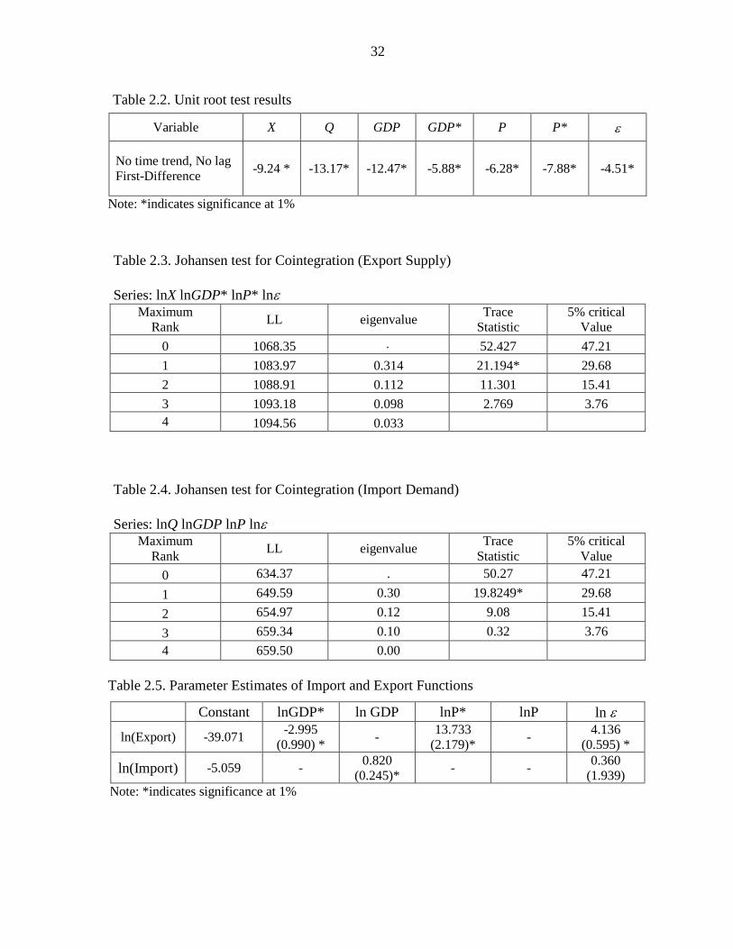
Table 2.2 Unit root test results .................................................................................. 32

Table 2.3. Johansen test for Cointegration (Export Supply) ...................................... 32

Table 2.4 Johansen test for Cointegration (Import Demand) ................................... 32

Table 2.5. Parameter Estimates of Import and Export Functions ............................. 32

Table 2.6 Tariff Equivalents of Devalued Yuan ....................................................... 33

Table 3.1. Variables in China and the Unites States .................................................. 66

Table 4.1 The values of parameters .......................................................................... 88

Table 4.2. The values of the steady state ................................................................... 88

vi

ACKNOWLEDGMENTS

Undertaking this PhD has been a truly life-changing experience for me and it would

not have been possible to do without the support and guidance that I received from many

people.

First, I would like to say a very big thank you to my advisor Professor E. Kwan Choi

for patiently guiding me in finishing this dissertation. Professor Choi provided me with every

bit of guidance, assistance, and expertise. When I felt ready to venture into research on my

own, he gave me valuable feedback, advice, and encouragement. In addition to our academic

collaboration, I greatly value the close personal rapport that Dr. Choi and I have forged over

the years. I quite simply cannot imagine a better adviser.

Second, I would like to thank Professor Rajesh Singh for his valuable instruction,

advice and supports during my PhD study at Iowa State University. Professor Singh intrigued

my interest in international economics. I secured my strict training in the usage of dynamic

methods. Moreover, during my struggling period, he also provided me sincere suggestions

and guidance to get over the frustrating obstacles. Meanwhile, my thanks also go to Professor

Peter F. Orazem, Professor Juan C. Cordoba, and Professor Paul W. Gallagher for agreeing

to be my committee members and supervising my research.

Third, I am indebted to Mam and Dad for always believing in me and encouraging me

to follow my dreams. And my sister and brother in law for helping in whatever way they

could during this challenging period.

Last but not least I am deeply thankful to my wife for her love, support, and

sacrifices. She has been my side throughout this Ph.D., living every single minute of it, and

vii

without whom, I would not have had the courage to embark on this journey in the first place.

To our two daughters Alexis and Genesis, their trust and supports are the source of

happiness, strength and wisdom in my life. I will achieve nothing without my wife and two

daughters.

viii

ABSTRACT

During the past decade, foreign exchange reserves of China and Japan have increased

dramatically. For instance, China’s foreign exchange reserve rose from $954.6 billion in

January 2007 to $3.5 trillion in April 2016. China and Japan seem to hold large foreign

reserves, much more than are necessary to facilitate their imports. The WTO regulates only

tariff and various non-tariff barriers but has made little effort to regulate the bilateral

exchange rates because exchange rate practices are within the purview of the IMF. At

present, the World Trade Organization (WTO) does not treat currency devaluation as a

protective trade policy. In my dissertation, I have chosen three topics in the area of

international economics. The first chapter argues that currency devaluation is equivalent to

an import tariff, and hence currency devaluation should be treated as a trade policy

instrument. The second chapter considers the employment effects of currency devaluations in

a Keynesian open economy. Currency devaluation may decrease domestic employment and

increase the social welfare. Under plausible conditions, the optimal policy is to get rid of

domestic unemployment in input sectors. The third chapter investigates the effects of public

capital investment in the export sector for the labor movement and capital formation and

identifies the contribution of public capital and other economic factors to the productivity

growth rate in the firm sector. We show that the optimal tariffs are positive but decrease to

the steady state level.

1

CHAPTER 1. INTRODUCTION

This dissertation addresses two main issues in international economics, currency

devaluation and import tariffs. John Maynard Keynes (1931, p.199) partly recognized the effect

of devaluation, when he argued that “Precisely the same effects as those produced by a

devaluation of sterling by a given percentage could be brought about by a tariff of the same

percentage on all imports together [italics added] with an equal subsidy on all exports…” The

second chapter shows whether yuan devaluations are equivalent to import tariffs in a two-good,

two-currency model. Even if no tariffs or quotas are employed, our analysis shows that a country

can restrict imports by undervaluing its currency. Contrary to Keynes’s statement, a 50 percent

devaluation from the benchmark exchange rate is shown to yield the same import price and

volume as a 100 percent tariff on imports without an export subsidy. Using the available yuan-

dollar exchange rates and bilateral U.S.-China trade data, it is shown that during the period 1994

- 2015, China’s yuan has been grossly undervalued. On average, the yuan was devalued by 45

percent, and the average of tariff equivalents of the undervalued yuan was 87.5 percent for the

period 1994-2015. The finding that tariffs and the undervalued yuan have the same effects on

domestic prices and import volumes.

During the past two decades, many Asian Counties have accumulated foreign exchange

reserves. For instance, China, Japan, and South Korea have accumulated $3.5 trillion, $1.32

trillion and $0.37 trillion as of April 2016, respectively. In developing countries, maintaining low

unemployment rate is far more important than other economic problems. Thus, the Chinese

government may adopt low yuan policy and accumulate foreign exchange reserves, not to take

2

advantage of its trading partners, but to reduce unemployment. Since the exchange rate pass-

through on the relative price of import good in the U.S. is not complete, The third chapter

investigates optimal exchange rate for a Keynesian open economy. We consider an open

economy that produces two tradable goods. In the benchmark equilibrium, all firms are price

takers and the yuan price of the dollar is determined by the demand and supply of traded goods.

Under a plausible scenario, the optimal yuan value of the dollar is less than that which ensures

full employment. China may pursue the low yuan policy to reduce domestic unemployment and

to maximize gross domestic product.

In many developing counties, lack of public infrastructures such as highways,

transportation, power and water system is slowing economic growth because the infrastructure

systems are crucial input factors for domestic production. Public investment plays an important

role and a major policy issue in developing countries. A number of studies support that public

capital has a powerful impact on the productivity of private capital. The fourth chapter addresses

the relationship between the government expenditure in public capital stock and economic

growth and examine an optimal import tariff for increase in public capital stock in a small open

economy. This practice explains rationale for government provision of public goods based on the

market failure, internalizes externalities in the private production function. Moreover, the paper

is alternatively answering "Why does the government devalue its own currency and change the

terms of trade in the short run? " The effect of change in exchange rate is the similar to that of

import tariffs which changes the relative price in domestic economy. This distortion of

government policy discourages current consumptions for import goods and encourage

consumptions of home goods and capital investments.

3

CHAPTER 2. TARIFF EQUIVALENTS OF CHINA’S UNERVALUED YUAN

2.1 Abstract

This paper considers a two-good, two-currency model to demonstrate that undervalued currency

is equivalent to an import tariff. Contrary to Keynes’s statement, a 50 percent devaluation from

the benchmark exchange rate is shown to yield the same import price and volume as a 100

percent tariff on imports without an export subsidy. A numerical example based on a Cobb-

Douglas utility function illustrates the main proposition. Using the Chinese trade data and U.S.

consumer price index, we show that China’s yuan was undervalued by 45 percent on average for

the period 1994-2015, and the average of equivalent tariffs was 87.5 percent on China’s imports.

2.2 Introduction

The People’s Bank of China (PBC), the central bank of China, began to regulate renminbi

on January 1, 1994 by moving the official rate to the then-prevailing swap market rates, which

contributed to the steady increase in China’s foreign exchange reserve (Goldstein and Lardy

2009). During the past two decades, China’s foreign exchange reserve rose significantly,

surpassing $3.3 trillion as of December 2015.

Those who investigated China’s yuan policy during the past ten years generally agreed

that the Chinese yuan has been undervalued, but their estimates of yuan undervaluation vary

widely. Funke and Rahn (2005) noted that in the aftermath of the Asian financial crisis, the yuan

was stabilized but undervalued by 15 percent in 1999. Gan et al. (2013) estimates he RMB

4

was undervalued by an average of 6.7 percent. In a multinational comparison of currency

undervaluation, Chang (2007) noted that the yuan was undervalued by 22 percent in 2001. Wren-

Lewis (2004) suggested a 20 percent devaluation of the yuan against the dollar in 2002, whereas

Coudert and Couharde (2007) reported that the bilateral renminbi-dollar exchange rate was

undervalued by 60 percent during the same year. Chang and Shao (2004) noted that RMB was

undervalued 22.5 percent in 2003. Claud Meyer (2008, p. 7) stated that “over the period 2002-

2007, the undervaluation of the RMB would be on this basis in the range of 10-15 percent

against the US$.” Garroway et al’s (2012) estimate of undervaluation in 2007 for renminbi was

15 percent. Referring to the current value of the yuan, Bergsten (2010) observed that “The

Chinese renminbi is undervalued by about 25 percent on a trade-weighted average basis and by

about 40 percent against the dollar.”

The dramatic rise in China’s cumulative trade surplus has spurred a debate concerning

China’s currency valuation and misalignment. The common view is that China has intentionally

depressed the value of its currency, the renminbi (RMB), to gain unfair advantages in the global

market.i (Cheung et al., 2009, Cheung, 2012).

These estimates of yuan undervaluation often are used to justify policy recommendations

to exert pressure on China to modify its currency policy. For example, Bergsten (2010) of the

Peterson Institute for International Economics recently suggested that the RMB must appreciate

by approximately 40 percent against the dollar to correct current “global imbalances” and urged

the United States to take multilateral, and if necessary unilateral action, to pressure China to

change its ways.

John Maynard Keynes (1931, p.199) partly recognized the effect of devaluation, when he

argued that “Precisely the same effects as those produced by a devaluation of sterling by a given

5

percentage could be brought about by a tariff of the same percentage on all imports together

[italics added] with an equal subsidy on all exports…” Also, Kong (2012) recognized that long-

term devaluation of a major currency such as the Chinese yuan may endanger the entire world

trading system.

By design the International Monetary Fund (IMF) is concerned with exchange rate

practices, while GATT /WTO is interested in regulating trade practices. Currency practices fall

within the purview of the IMF, and are generally considered to be outside the jurisdiction of the

WTO. Although currency devaluation affects international trade, the WTO has made little effort

to regulate the exchange rate practices of member countries because any such attempt may be

viewed as “intruding into the domain of the IMF.” (Kong, 2012, p. 112) While the two

institutions complement each other, neither institution has been willing to take actions on

currency practices that have spillover effects on world trade. Hence, the hesitation of the IMF to

take action against countries that manipulate exchange rates to gain “unfair advantage” over their

trading partners.

Section 2.3 presents the basic model of two goods and two currencies, and Section 2.4

investigates the equivalence of devaluations and tariffs. Section 2.5 provides graphical

illustrations of the effects of devaluation, while Section 2.6 uses a numerical example with a

Cobb-Douglas utility function. Section 2.7 provides empirical estimates of China’s import

demand and export supply function, which yield estimates of yuan devaluations for the period

1994-2015, and Section 2.8 offers concluding remarks.

6

2.3 The Basic Model

In order to compare the effects China’s tariffs and currency devaluation on trade, we first

construct a basic model with two goods and two currencies. There are two countries, the home

country, China, and the foreign country, the United States. We employ the following

assumptions to describe the production side of China’s economy:

(i) Supplies of the two tradable goods are subject to the production possibility function (PPF),

( )C F Z= , where C and Z are the outputs of the exportable and the importable.

(ii) Each country fixes the price of its exportable good, i.e., the yuan price b of good C is fixed in

China, and the dollar price P* of good Z is fixed in the United States.

(iii) Perfect competition prevails in the domestic product and resources are fully employed.

Let ε denote the dollar price of Chinese yuan, and P be the yuan price of the importable

good Z. China fixes the yuan price of its exportable good C, and the United States also fixes the

dollar price of its exportable (good Z). That is, the yuan price b of good C and the dollar price

*P Pε= of good Z are fixed and remain unaltered whether a tariff is imposed or the yuan is

devalued. If no tariff is imposed, the relative price of the importable in China is / * / .P b P bε=

Let c and z denote the domestic consumption of the exportable and importable, and let x and q

denote the physical volumes of exports and imports. Then x C c= − and .q z Z= − The dollar

value of imports is *qP .

Domestic producers are assumed to maximize yuan revenue ( ) ,R bF Z PZ= + where

1,b = since the exportable is the numéraire. The first order condition for revenue maximization

requires

7

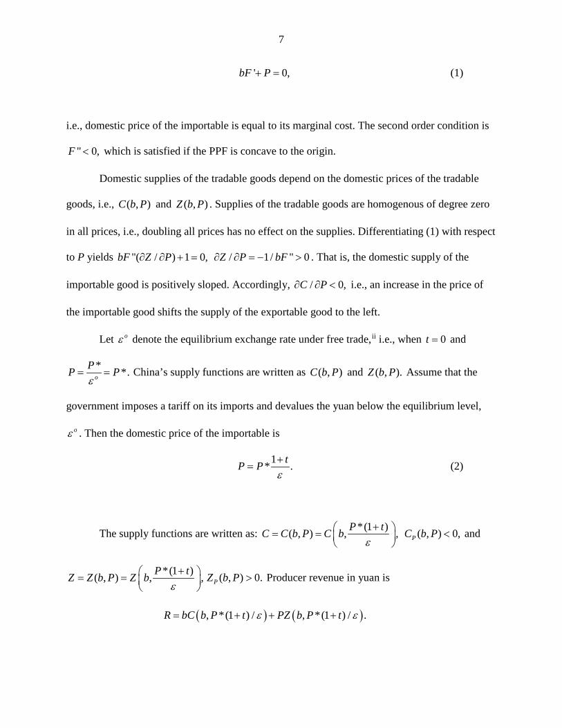
' 0,bF P+ = (1)

i.e., domestic price of the importable is equal to its marginal cost. The second order condition is

" 0,F < which is satisfied if the PPF is concave to the origin.

Domestic supplies of the tradable goods depend on the domestic prices of the tradable

goods, i.e., ( , )C b P and ( , )Z b P . Supplies of the tradable goods are homogenous of degree zero

in all prices, i.e., doubling all prices has no effect on the supplies. Differentiating (1) with respect

to P yields "( / ) 1 0,bF Z P∂ ∂ + = / 1/ " 0Z P bF∂ ∂ = − > . That is, the domestic supply of the

importable good is positively sloped. Accordingly, / 0,C P∂ ∂ < i.e., an increase in the price of

the importable good shifts the supply of the exportable good to the left.

Let oε denote the equilibrium exchange rate under free trade,ii i.e., when 0t = and

* *.o

PP Pε

= = China’s supply functions are written as ( , )C b P and ( , ).Z b P Assume that the

government imposes a tariff on its imports and devalues the yuan below the equilibrium level,

oε . Then the domestic price of the importable is

1* .tP Pε+

= (2)

The supply functions are written as: *(1 )( , ) , ,P tC C b P C bε+ = =

( , ) 0,PC b P < and

*(1 )( , ) , ,P tZ Z b P Z bε+ = =

( , ) 0.PZ b P > Producer revenue in yuan is

( ) ( ), *(1 ) / , *(1 ) / .R bC b P t PZ b P tε ε= + + +

8

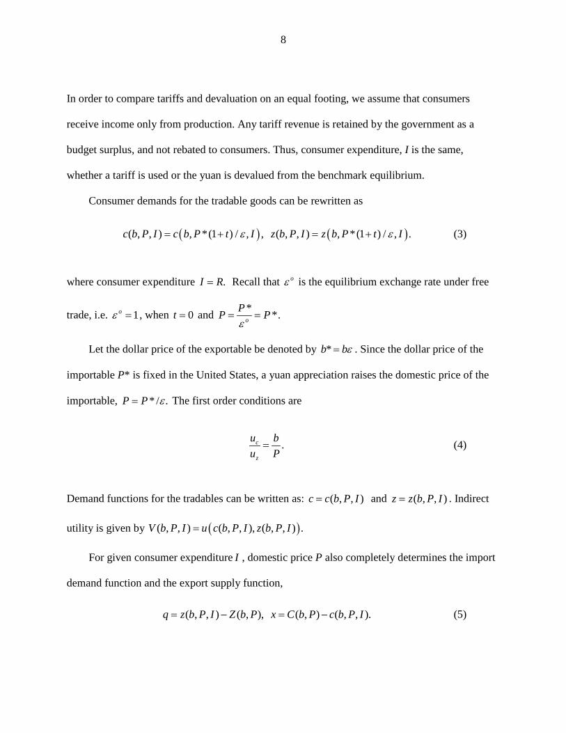
In order to compare tariffs and devaluation on an equal footing, we assume that consumers

receive income only from production. Any tariff revenue is retained by the government as a

budget surplus, and not rebated to consumers. Thus, consumer expenditure, I is the same,

whether a tariff is used or the yuan is devalued from the benchmark equilibrium.

Consumer demands for the tradable goods can be rewritten as

( ) ( )( , , ) , *(1 ) / , , ( , , ) , *(1 ) / , .c b P I c b P t I z b P I z b P t Iε ε= + = + (3)

where consumer expenditure .I R= Recall that oε is the equilibrium exchange rate under free

trade, i.e. 1oε = , when 0t = and * *.o

PP Pε

= =

Let the dollar price of the exportable be denoted by *b bε= . Since the dollar price of the

importable P* is fixed in the United States, a yuan appreciation raises the domestic price of the

importable, * / .P P ε= The first order conditions are

.c

z

u bu P

= (4)

Demand functions for the tradables can be written as: ( , , )c c b P I= and ( , , )z z b P I= . Indirect

utility is given by ( )( , , ) ( , , ), ( , , ) .V b P I u c b P I z b P I=

For given consumer expenditure I , domestic price P also completely determines the import

demand function and the export supply function,

( , , ) ( , ), ( , ) ( , , ).q z b P I Z b P x C b P c b P I= − = − (5)

9

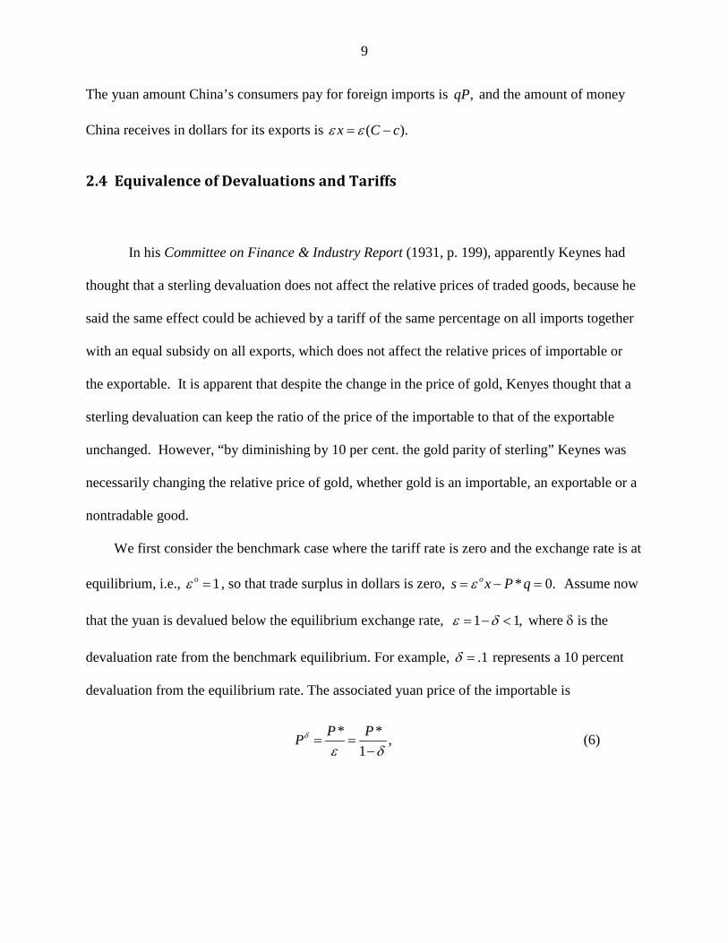
The yuan amount China’s consumers pay for foreign imports is ,qP and the amount of money

China receives in dollars for its exports is ( ).x C cε ε= −

2.4 Equivalence of Devaluations and Tariffs

In his Committee on Finance & Industry Report (1931, p. 199), apparently Keynes had

thought that a sterling devaluation does not affect the relative prices of traded goods, because he

said the same effect could be achieved by a tariff of the same percentage on all imports together

with an equal subsidy on all exports, which does not affect the relative prices of importable or

the exportable. It is apparent that despite the change in the price of gold, Kenyes thought that a

sterling devaluation can keep the ratio of the price of the importable to that of the exportable

unchanged. However, “by diminishing by 10 per cent. the gold parity of sterling” Keynes was

necessarily changing the relative price of gold, whether gold is an importable, an exportable or a

nontradable good.

We first consider the benchmark case where the tariff rate is zero and the exchange rate is at

equilibrium, i.e., 1oε = , so that trade surplus in dollars is zero, * 0.os x P qε= − = Assume now

that the yuan is devalued below the equilibrium exchange rate, 1 1,ε δ= − < where δ is the

devaluation rate from the benchmark equilibrium. For example, .1δ = represents a 10 percent

devaluation from the equilibrium rate. The associated yuan price of the importable is

* * ,1

P PPδ

ε δ= =

−(6)

10

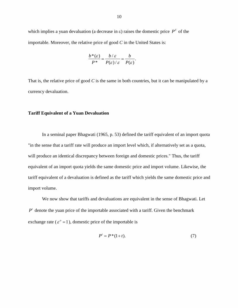
which implies a yuan devaluation (a decrease in ε) raises the domestic price Pδ of the

importable. Moreover, the relative price of good C in the United States is:

*( ) / .* ( ) / ( )

b b bP P Pε ε

ε ε ε= =

That is, the relative price of good C is the same in both countries, but it can be manipulated by a

currency devaluation.

Tariff Equivalent of a Yuan Devaluation

In a seminal paper Bhagwati (1965, p. 53) defined the tariff equivalent of an import quota

"in the sense that a tariff rate will produce an import level which, if alternatively set as a quota,

will produce an identical discrepancy between foreign and domestic prices." Thus, the tariff

equivalent of an import quota yields the same domestic price and import volume. Likewise, the

tariff equivalent of a devaluation is defined as the tariff which yields the same domestic price and

import volume.

We now show that tariffs and devaluations are equivalent in the sense of Bhagwati. Let

tP denote the yuan price of the importable associated with a tariff. Given the benchmark

exchange rate ( 1oε = ), domestic price of the importable is

*(1 ).tP P t= + (7)

11

The yuan-dollar exchange rate when the yuan is devalued from the benchmark rate 1oε = is

1 .ε δ= − A tariff rate t is equivalent to a 100 δ× percent devaluation, if the same domestic price

is achieved through the tariff, i.e.,

*.t PP Pδ

ε= = (8)

Thus, the tariff equivalent of a given exchange rate ε is:

1 .t εε−

= (9)

For instance, a 10 percent devaluation is equivalent to an 11 percent tariff, i.e.,

.1/ .9 11.11%t = = .

Effects on Production and Consumer Income

When a tariff is imposed and 1ε = , the supply of the importable is:

( )( , ) , *(1 ) ,tZ b P Z b P t= + where tP is the yuan price of good Z when an import tariff t is

imposed. When a devaluation occurs, ( , ) ( , * / ),Z b P Z b Pδ ε= where Pδ is the yuan price of Z

when the rate of yuan devaluation is δ. Recall that the supply of the importable, ( , )Z b P , is

monotone increasing in P. Thus, ( ) ( ), *(1 ) , * /Z b P t Z b P ε+ = if, and only if *(1 ) * / ,P t P ε+ =

or 1 .1 t

ε =+

That is, the import volume of Z remains the same, whether a devaluation,

11

tt

δ ε= − =+

, occurs, or its equivalent tariff is imposed. Likewise, under both regimes

12

domestic production of the exportable is the same, ( , ) ( , )tC b P C b Pδ= , as is the yuan value of

China’s income,

( , ) ( , ) ( , ) ( , ) .t t t tR bC b P P Z b P bC b P P Z b P Rδ δ δ δ≡ + = + ≡

Thus, when ,1

tt

δ =+

consumers have the same income, ,tI I δ= equal to producer revenue,

tR Rδ= under both regimes.

Effects on Import Volume

Recall from (5), the import demand function is ( , , ) ( , , ) ( , )q b P I z b P I Z b P= − . Since all

prices and income are the same under both regimes, consumer demands for the exportable and

the importable are the same, ( , , ) ( , , )t tc b P I c b P Iδ δ= and z( , ) ( , ).t tP I z P Iδ δ= The import

demand function with a tariff is given by ( , , ) ( , ).t t t tq z b P I Z b P= − Likewise, the import

demand function with the devalued yuan is ( , , ) ( , ).q z b P I Z b Pδ δ δ δ= − Thus, the import

volumes are the same under both regimes, i.e., ( , , ) ( , , )t tq b P I q b P Iδ δ= . Since both t and δ yield

the same domestic prices and the same volume of imports, there exists a tariff that is equivalent

to any yuan devaluation, and vice versa.

Proposition 1: Suppose the government devalues the yuan below the benchmark equilibrium

exchange rate, 1oε = . Then the domestic price rises above the import price to *PPδ

ε= , and

13

import volume falls to .qδ The tariff equivalent, 1t εε−

= , yields the same domestic price,

tP Pδ= and the same import volume, .tq qδ=

The relationship between an exchange rate and its equivalent tariff in (9) can be written as:

.1

t δδ

=−

(10)

This shows that a yuan devaluation is more potent than an equal tariff. That is, a 10 percent yuan

devaluation from the benchmark rate is more restrictive than an equal tariff rate in reducing the

import volume. Alternatively, if an import tariff of 10 percent is used to restrict imports, the

same volume of import can be achieved by less than a 10 percent devaluation of the yuan, since

from (10), we have

.1

t tt

δ = <+

(11)

For instance, a 50 percent devaluation ( 1 0.5δ ε= − = ) from the equilibrium exchange rate

1oε = is equivalent to a 100 percent tariff, and domestic price rises 100 percent with the same

volume of import in both regimes. Likewise, a 20 percent yuan devaluation is equivalent to a 25

percent tariff.

Tariff cum Devaluation

Next, consider the case where the yuan is devalued and a tariff is imposed simultaneously.

In this case, domestic price rises to: 1* .tP Pε+

= We now show that a pairing ( , )t ε of a tariff

14

and an exchange rate is equivalent to a single tariff τ. Since both instruments yield the same

domestic prices, the tariff equivalent of a joint tariff cum devaluation is defined by

1*(1 ) * ,tP Pτε+

+ = or 11 .tτε+

+ = That is, an import tariff cum devaluation is equivalent to a

single tariff τ. Notice that the single tariff exceeds the sum of the tariff rate and the rate of yuan

devaluation,

.1t tδτ δ

δ+

= > +−

(12)

Moreover, when both are used, the total effect on the import price is superadditive, i.e., a 10

percent devaluation plus a 10 percent tariff is equivalent to a single tariff of 22.22 percent.

2.5 Graphical Illustration

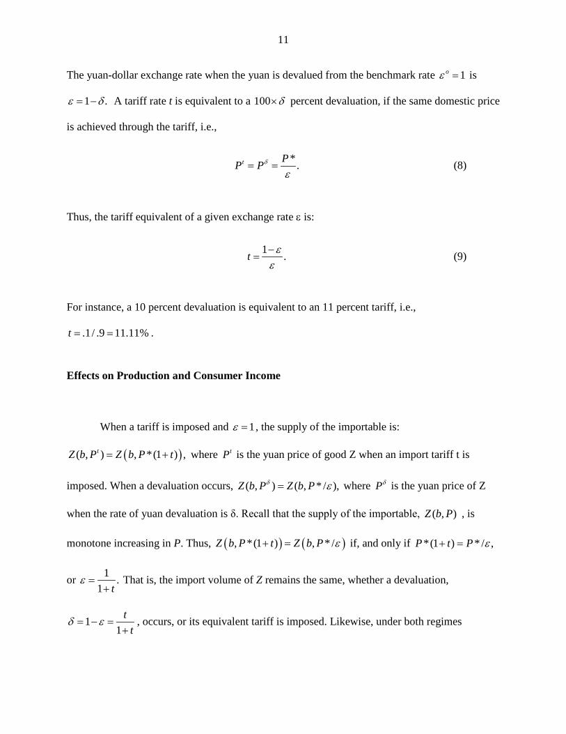
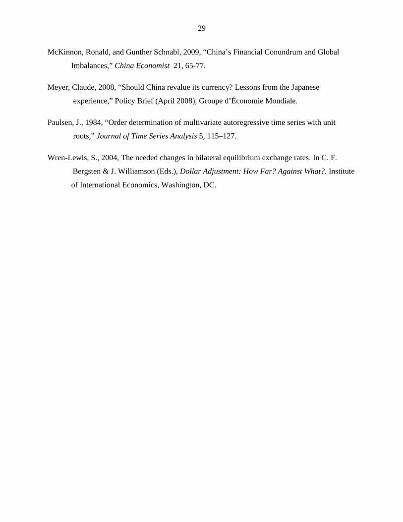
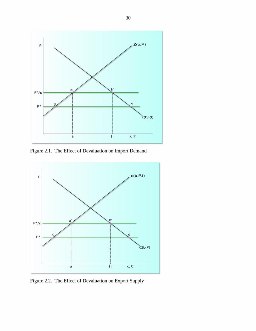
The effect of currency devaluation on imports is shown in Figure 2.1. Note that demand

for the importable z depends on P and revenue R, which in turn depends on the domestic price P.

Assume both the exportable and importable are normal goods. For the purpose of graphical

illustration, we employ reduced form demand functions which incorporate the income effects.

The reduced form demand functions for the importable and the exportable

are: ( )( , ) , , ( , )z b P z b P R b P≡ and ( )( , ) , , ( , ) .c b P c b P R b P≡ An increase in P not only decreases

the quantity of the importable demanded, but also raises producer revenue or income R, which

partially offsets the direct effect. We assume that the direct effect is dominant, i.e.,

( , ) / 0.z b P P∂ ∂ <

15

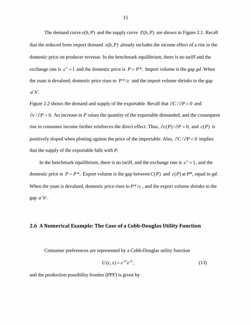
The demand curve ( , )z b P and the supply curve ( , )Z b P are shown in Figure 2.1. Recall

that the reduced form import demand ( , )z b P already includes the income effect of a rise in the

domestic price on producer revenue. In the benchmark equilibrium, there is no tariff and the

exchange rate is 1oε = and the domestic price is *.P P= Import volume is the gap gd. When

the yuan is devalued, domestic price rises to * /P ε and the import volume shrinks to the gap

' '.a h

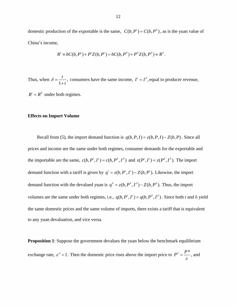
Figure 2.2 shows the demand and supply of the exportable. Recall that / 0C P∂ ∂ < and

/ 0.c P∂ ∂ > An increase in P raises the quantity of the exportable demanded, and the consequent

rise in consumer income further reinforces the direct effect. Thus, ( ) / 0,c P P∂ ∂ > and ( )c P is

positively sloped when plotting against the price of the importable. Also, / 0C P∂ ∂ < implies

that the supply of the exportable falls with P.

In the benchmark equilibrium, there is no tariff, and the exchange rate is 1oε = , and the

domestic price is *.P P= Export volume is the gap between ( )C P and ( )c P at P*, equal to gd.

When the yuan is devalued, domestic price rises to * /P ε , and the export volume shrinks to the

gap ' '.a h

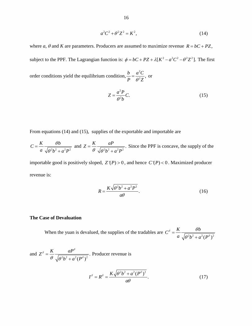
2.6 A Numerical Example: The Case of a Cobb-Douglas Utility Function

Consumer preferences are represented by a Cobb-Douglas utility function

.25 .25( , ) ,U c z c z= (13)

and the production possibility frontier (PPF) is given by

16

2 2 2 2 2 ,a C Z Kθ+ = (14)

where a, θ and K are parameters. Producers are assumed to maximize revenue ,R bC PZ= +

subject to the PPF. The Lagrangian function is: 2 2 2 2 2[ ].bC PZ K a C Zφ λ θ= + + − − The first

order conditions yield the equilibrium condition,2

2 ,b a CP Zθ= or

2

2 .a PZ Cbθ

= (15)

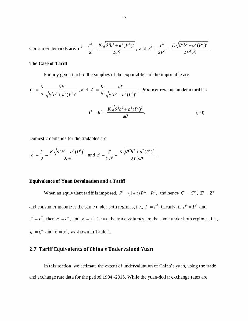
From equations (14) and (15), supplies of the exportable and importable are

2 2 2 2

K bCa b a P

θθ

=+

and 2 2 2 2

.K aPZb a Pθ θ

=+

Since the PPF is concave, the supply of the

importable good is positively sloped, '( ) 0Z P > , and hence '( ) 0C P < . Maximized producer

revenue is:

2 2 2 2

.K b a PRa

θθ+

= (16)

The Case of Devaluation

When the yuan is devalued, the supplies of the tradables are 2 2 2 2( )

K bCa b a P

δ

δ

θθ

=+

and 2 2 2 2

.( )

K aPZb a P

δδ

δθ θ=

+ Producer revenue is

2 2 2 2( )

.K b a P

I Ra

δδ δ θ

θ+

= = (17)

17

Consumer demands are: 2 2 2 2( )

,2 2

K b a PIca

δδδ θ

θ+

= = and 2 2 2 2( )

.2 2

K b a PIzP P a

δδδ

δ δ

θθ

+= =

The Case of Tariff

For any given tariff t, the supplies of the exportable and the importable are:

2 2 2 2( )t

t

K bCa b a P

θθ

=+

, and 2 2 2 2

.( )

tt

t

K aPZb a Pθ θ

=+

Producer revenue under a tariff is

2 2 2 2( )

.t

t t K b a PI R

aθ

θ+

= = (18)

Domestic demands for the tradables are:

2 2 2 2( )

2 2

ttt K b a PIc

aθ

θ+

= = and 2 2 2 2( )

.2 2

ttt

t t

K b a PIzP P a

θθ

+= =

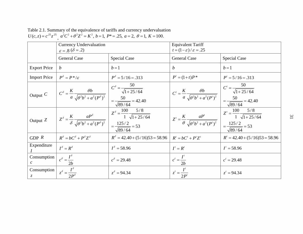
Equivalence of Yuan Devaluation and a Tariff

When an equivalent tariff is imposed, ( )1 * ,tP t P Pδ+ == and hence tC Cδ= , tZ Z δ=

and consumer income is the same under both regimes, i.e., .tI I δ= Clearly, if tP Pδ= and

,tI I δ= then tc cδ= , and .tz zδ= Thus, the trade volumes are the same under both regimes, i.e.,

tq qδ= and ,tx xδ= as shown in Table 1.

2.7 Tariff Equivalents of China’s Undervalued Yuan

In this section, we estimate the extent of undervaluation of China’s yuan, using the trade

and exchange rate data for the period 1994 -2015. While the yuan-dollar exchange rates are

18

available in monthly data, the import and export statistics are quarterly data. Thus, the exchange

rate of the last month of each quarter is used as the exchange rate of each quarter. China GDP

data is obtained from the National Bureau of Statistics of China, while U.S. GDP data is from the

Bureau of Labor Statistics. We also utilized the monthly data for Sino-US bilateral trade in goods

from the US census (https://www.census.gov/foreign-trade/balance/c5700.html). China’s

monthly nominal exchange rates are obtained from the State Administration of Foreign

Exchange (SAFE) of the People's Republic of China, while Consumer Price Index (CPI) for the

United States and China are from the OECD (https://data.oecd.org/price/inflation-cpi.htm).

VAR (Vector Autoregressive) and VECM (Vector Error Correction Model) are most

often used to find relationships with two or more endogenous variables. Even though variables

are individually non-stationary, they may be cointegrated. For instance, export, income and

exchange rate may have one cointegrating relationship. We employ Johansen’s (1998) Vector

Error Correction Model (VECM) to explore the long-term relationships and short-term dynamics

among endogenous variables. The model shows that in the long run, endogenous variables

converge to their cointegrated relations. The long run relationships are investigated in three steps.

First, the order of integration of variables is determined by Augmented Dickey Fuller test (ADF).

Second, if each variable is integrated in the same order, i.e., I(1), a sequence test (Johansen 1995)

is performed to determine the cointegrating rank r which indicates the maximum possible

number of cointegrated equations. We test the null hypothesis of 0r = against 1r ≥ to

determine whether there is one cointegrating relationship. If the hypothesis of 0r = is rejected,

there is no relationship among the variables and there is no need for VECM, in which case, a

VAR model can be employed. Finally, if there exist cointegrated relationships, then Johansen’s

19

cointegration test is used to detect long term relationships between exports (imports) and

exchange rate.

Consider China’s import expenditure and export revenue functions,

* *( , , )t t t tX g GDP P ε= and ( , , )t t t tQ f GDP P ε= , where tGDP is China’s gross domestic income

(GDP), *tGDP is the United States’ GDP, P* is the US CPI, P is Chinese CPI and tε is the dollar

price of the yuan. This model is similar to Bahmani-Oskooee and Ardalani (2006) model which

employed real effective exchange rate rather than CPI and nominal exchange rate.

The dollar values of exports (X) and imports (Q) are written as:

* *1 2 3ln ln ln ,t o t t t XtX GDP Pα α α α ε ω= + + + + (19)

1 2 3ln ln ln ,t o t t t QtQ GDP Pβ β β β ε ω= + + + + (20)

where α’s and β’s are unknown parameters and Xtω and Qtω are error terms with zero mean and

variances 2Xσ and 2

Qσ , respectively. Our analysis suggests that 2 ,α and 1β are positive while

2β and 3β are negative. However, 1α may be negative or positive, depending on the

characteristics of the exportable goods of China. If China’s export is a normal (inferior) good,

then 1α is positive (negative).

We estimate the long-run relations between US-China bilateral trade and the exchange

rate, using cointegration and error-correction modeling.

Unit Root Test

We examine the stochastic properties of the variables using Dickey and Fuller (1981)

tests of unit roots. Unit root tests are based on estimating the following univariate models:

20

0 1 ( 1) 12

p

t t i t i ti

y y yα α β ε− − +=

∆ = + + +∑ (21)

0 1 ( 1) 122

p

t t i t i ti

ty y yα α α β ε− − +=

∆ = + + + +∑ (22)

where y is the variable to be tested for unit roots and t is the time trend. Equation (21) tests for

unit roots around a constant, while equation (22) tests for unit roots around a constant and

deterministic trend. The lag lengths, p, are chosen using Schwarz’s information criterion. Under

the null hypothesis, 1: 0oH α = implies that the variable has a unit root.

Cointegration Tests

Tests of cointegration under symmetric adjustment are based on the methodology

developed by Johansen (1991), and Johansen and Juselius (1993). Johansen's method is to test

the restrictions imposed by cointegration on the unrestricted VAR, involving the series. The

mathematical form of a VAR is

1 1t o t p t p t ty A A y A y Bx ω− −= + + + + + (23)

where ty is an n-vector of non-stationary I(1) variables, tx is a d-vector of deterministic

variables, 1,A …, pA and B are matrices of coefficients to be estimated, and tε is a vector of

innovations that may be contemporaneously correlated with each other. However, they are

uncorrelated with their own lagged values and other right-hand side variables.

The corresponding vector error correction model can be written as,

1 1 1 .t o t p t p t t ty B B y B y B x y vπ− − −∆ = + ∆ + + ∆ + ∆ + + (24)

21

Granger’s representation theorem asserts that if the coefficient matrix π has a reduced rank

r n< , then there exist n r× matrices, α , and β , each with rank r such that 'π αβ= and ' tyβ

are stationary. Here, r is the number of cointegrating relations, and each column of β is a

cointegrating vector. For n endogenous non-stationary variables, there can be from (0) to (n-1)

linearly independent, cointegrating relations. Cointegration implies the existence of stable

relations among the variables in the model, and causality in at least one direction. The Error

Correction Model (ECM) is used to test for the direction of causality in both short- and long-run

(Engle and Granger, 1987). Thus, we examine causality between exports (or imports) and the

nominal exchange rate using their corresponding ECM models. In particular, we are interested

in the following two error-correction models associated with import demand and export supply

function:

The export supply is given by:

1 1 *1 1 1 1

1 1

1 * 12 3

1 1

ln ln ln

ln ln ,

n n

t Xt i t i i t ii i

n n

i t i i t ii i

X ECT X GDP

P

α λ θ θ

θ θ ε

− −= =

− −= =

∆ = + + ∆ + ∆

+ ∆ + ∆

∑ ∑

∑ ∑(25)

and the import demand is written as:

2 21 2 1 1 1

1 1

2 22 1 3

1 1

ln ln ln

ln ln ,

n n

t Xt i t i i ti i

n n

i t i t ii i

Q ECT Q GDP

P

β λ θ θ

θ θ ε

− −= =

− −= =

∆ = + + ∆ + ∆

+ ∆ + ∆

∑ ∑

∑ ∑(26)

where ECT is the error correction term, derived from the long-run cointegration relationship and

measures the magnitude of the past disequilibrium. In each equation, the change in the left-hand side

22

(LHS) variable is caused by past changes in the variable itself, past changes in other variables, as well as a

fraction 2λ of the previous equilibrium error. Given these specifications, the presence of short-run and

long-run causality could be tested.

Empirical Results

The results of the unit root tests for series of Exports (X), Imports (Q), Chinese GDP

(GDP), U.S. GDP (GDP*), Chinese CPI (P), U.S. CPI (P*) and the yuan value per dollar (ε)

using ADF are reported in Table 2.2. The null hypothesis that the variables are non-stationary in

level is not rejected across all variables. However, the null hypothesis of non-stationarity in

first-difference of variables is rejected for all variables. Thus, all variables appear to be non-

stationary in level and stationary after first differencing. Using the method of Paulsen (1984), the

optimal lags of VEC model are 4 lags in the export supply model and 2 lags in the import supply

model.

Table 2.3 and Table 2.4 show that the results of the Johansen Cointegration tests for the

export supply and import demand. In both models, the trace and maximum eigenvalue tests show

that the null hypothesis of the absence of cointegrating relation (r = 0) can be rejected at 5%

level of significance. Similarly, the null hypothesis of the existence of at most one cointegrating

relation (r ≤1) cannot be rejected at 5% level of significance. In short, both tests suggest the

existence of one cointegrating vectors driving the series with four common stochastic trends in

the data. Thus, we can conclude that the variables in both models are cointegrated. That is, there

is a long-run relationship among the export supply (or import demand), exchange rate, price or

income. In Table 2.5, the long term cointegrating vector suggests that Chinese exports have

23

causal relationships with U.S. income, U.S. domestic price and exchange rate. However, the

VEC model does not support the long run relationships between Chinese imports and the

exchange rate or China’s domestic prices. These results show that the exchange rate has no effect

on imports in the long run. Thus, there is no need to estimate the relationship between China’s

import demand and the exchange rate. The leading Chinese imports are electronic equipment, oil,

and machinery, and demand for these industrial products tend to be price inelastic. Thus, only the

coefficient of GDP is positive and significant at 1% confidence level.

The estimated long-run relationship in the export supply function is

ˆ ˆ39.071 2.995ln * 13.733ln *ˆl 4.136ln n .GDPX P ε− − + += (27)

The coefficients of U.S. domestic price and the exchange rate are positive. This implies that as

the prices of China’s domestic goods rise and the yuan depreciates, China’s export supply

increases. However, the coefficient of U.S. GDP is negative. This indicates that China’s

exportable goods are inferior goods. That is, as U.S. GDP rises, U.S. imports of China’s export

goods fall. Moreover, the results show that the elasticities of Chinese exports with respect to U.S

GDP, U.S. domestic price, and the exchange rate are all greater than unity. For instance, a 1-

percent increase in the exchange rate and the domestic price level increases China’s exports by

4.136% and 13.733%, respectively. Similarly, a 1-percent increase in U.S. GDP reduces China’s

exports by 2.995%.

All parameters are statistically significant at the 1-percent level. The estimated value of

exports is given by 0 31 2ˆ ˆˆ ˆ* *ˆ e ,t t t tX GDP Pα αα α ε= where 0α̂ , 1α̂ , 2α̂ ,and 3α̂ are estimated parameters

24

in equation (19), and e 2.71828= is the base of the natural logarithm. Since Chinese imports are

mostly derived demands for industrial inputs, rather than consumption demands, we use China’s

actual import data Q, instead of estimating the import demand function. In other words, China’s

import demand is not responsive to changes in the exchange rates. Thus, the estimated

equilibrium exchange rate *t̂ε at time t that yields bilateral trade balance is derived from the

condition,iii 0 31 2ˆ ˆˆ ˆ* *ˆ et t t t tX GDP P Qα αα α ε= = , and is written as

3

0 1 2

ˆ1/*

ˆ ˆ ˆ* *ˆ ,

ett t

QGDP P

α

α α αε

=

(28)

From the estimated equilibrium exchange rates in (28) and actual exchange rates, the rate of

devaluation in period t is given by

ˆˆ ,ˆ

t tt

t

ε εδε

−=

(29)

and the equivalent tariff rate in period t is given by

ˆ.ˆ1

tt

t

δτδ

= −

(30)

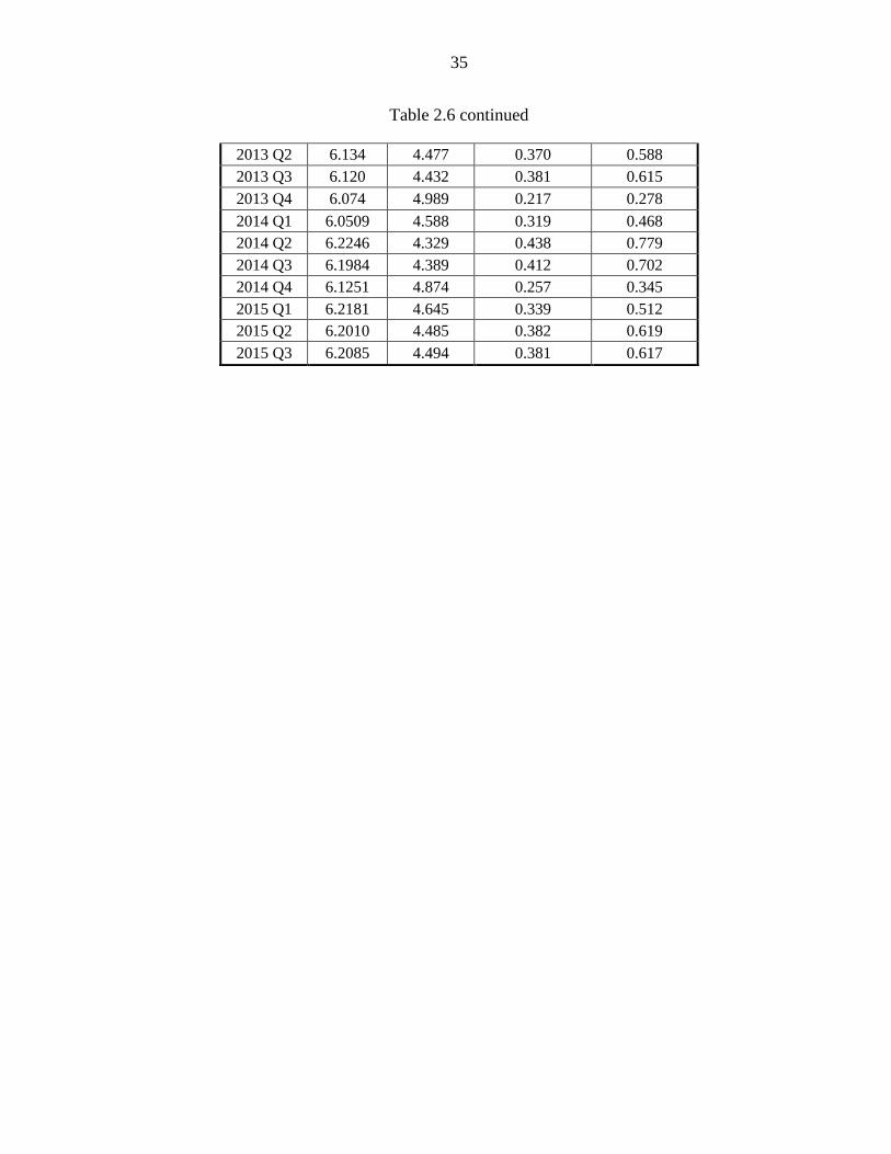
The quarterly equilibrium and actual exchange rates are shown in Table 2.6. For instance,

in the fourth quarter of 1994, the actual exchange rate was 8.5, which indicates a 47.9 percent

devaluation of the yuan below the equilibrium rate of 5.7. This undervaluation of the yuan is

equivalent to an import tariff of 92.1 percent. The rate of devaluation ranged from 21.7 percent

25

in the fourth quarter of 2013 to 63.9 percent in the first quarter of 2000. The corresponding tariff

equivalent ranged from 27.8 percent to 176.8 percent during the same period. The average rate of

devaluation from the equilibrium exchange rates was 45.1 percent, and the average of equivalent

tariffs was 87.5 percent.

2.8 Concluding Remarks

While tariffs and non-tariff barriers are bound by various agreements in the WTO, there

are no such agreements among countries on the bilateral exchange rates. The IMF tends to

monitor only the exchange rates of developing countries that are beset by large balance of

payments deficits. The WTO regulates only tariff and various non-tariff barriers, but has made

little attempt to regulate the bilateral exchange rates because exchange rate practices are within

the purview of the IMF.

This paper has shown that yuan devaluations are equivalent to import tariffs in a two-

good, two-currency model of international trade and exchange rates. Even if no tariffs or quotas

are employed, our analysis shows that a country can restrict imports by undervaluing its

currency. Using the available yuan-dollar exchange rates and bilateral U.S.-China trade data, it is

shown that during the period 1994 - 2015, China’s yuan has been grossly undervalued. On

average, the yuan was devalued by 45 percent, and the average of tariff equivalents of the

undervalued yuan was 87.5 percent for the period 1994-2015.

The finding that tariffs and the undervalued yuan have the same effects on domestic

prices and import volumes suggests that currency pegging can be viewed as a trade policy. Either

26

the WTO or IMF could begin to consider regulation of currency practices of developing

countries in the face of large trade imbalances between major trading countries.

27

2.9 References

Bahmani-Oskooee, M., and Z. Ardalani, 2006, “Exchange Rate Sensitivity of U.S. Trade

Flows: Evidence from Industry Data,” Southern Economic Journal 72, 542–559.

Bergsten, C. F., 2007, “The Dollar and the Renminbi,” Statement before the Hearing on US

Economic Relations with China: Strategies and Options on Exchange Rates and Market

Access, Subcommittee on Security and International Trade and Finance, Committee on

Banking, Housing and Urban Affairs, United States Senate, 23 May 2007.

Bergsten, C. F., 2010, “Correcting the Chinese exchange rate: An action plan,” Testimony

before the Committee on Ways and Means, U.S. House of Representatives, Peterson

Institute for International Economics,

http://www.iie.com/publications/testimony/testimony.cfm?ResearchID=1523 (24.3.10),

accessed November 25, 2014.

Bhagwati, Jagdish, 1965, “On the Equivalence of Tariffs and Quotas,” in R. E. Baldwin and

others (eds.), Trade, Growth, and the Balance of Payments- Essays in Honor of Gottfried

Haberler, Rand McNally and Company, Chicago.

Bhagwati, J., 1968, “More on the Equivalence of Tariffs and Quotas,” American Economic

Review 58, 142-46.

Chang, G. H., and Shao, Q., 2004, “How much is the Chinese currency undervalued? A

quantitative estimation,” China Economic Review 15, 366–71.

Chang, G. H., 2007, “Is the Chinese currency undervalued? Empirical evidence and policy

implication,” International Journal of Public Administration 30, 137–148.

Cheung, Yin-Wong, 2012, “Exchange Rate Misalignment –The Case of the Chinese

Renminbi,” Handbook of Exchange Rates, Jessica James, Ian W. Marsh and Lucio Sarno

(eds.).

Choi, E. Kwan, and Hailong Jin, 2013, “Currency Intervention and Consumer Welfare in an Open Economy." International Review of Economics and Finance 29, 47-56

28

Coudert, Virginie and Cécile Couharde, 2007, “Real Equilibrium Exchange Rate in China: Is

the Renminbi Undervalued?,” Journal of Asian Economics 18, 568-594.

Engle, R.F. and Granger, C.W.J., 1987, “Co-integration and Error Correction:

Representation, Estimation, and Testing”, Econometrica, 55, 251-276.

Fernalda, John, Edison, Hali, and Lounganib, Prakash, 1999, “Was China the first domino?

Assessing links between China and other Asian economies,” Journal of International

Money and Finance, 18, 515–535.

Funke, M., and Rahn, J., 2005, “Just how undervalued is the Chinese Renminbi?” World

Economy 28, 465–489.

Garroway, Christopher, Burcu Hacibedel, Helmut Reisen, and Edouard Turkisch, 2012, “The

Renminbi and Poor Country Growth,” World Economy 35, 273-94

Johansen, S., 1988, “Statistical analysis of cointegration vectors” Journal of Economic

Dynamics and Control 12, 231–254.

Johansen, S., 1995, “Likelihood-Based Inference in Cointegrated Vector Autoregressive

Models,” Oxford University Press.

Jin, Hailong, and E. Kwan Choi, 2013, “Profits and Losses from Currency Intervention,”

International Review of Economics and Finance 27, 14-20.

Jin, Hailong, and Choi, E. Kwan, 2014, “China’s Profits and Losses from Currency

Intervention, 1994-2011,” Pacific Economic Review 19, 170-183.

Keynes, John Maynard, 1931, Committee on Finance & Industry Report, June

1931Addendum, Macmillan Report.

Kong, Qingjiang, 2012, “China's Currency Devaluation and WTO Issues,” China: An

International Journal 10, 110-118.

29

McKinnon, Ronald, and Gunther Schnabl, 2009, “China’s Financial Conundrum and Global

Imbalances,” China Economist 21, 65-77.

Meyer, Claude, 2008, “Should China revalue its currency? Lessons from the Japanese

experience,” Policy Brief (April 2008), Groupe d’Économie Mondiale.

Paulsen, J., 1984, “Order determination of multivariate autoregressive time series with unit

roots,” Journal of Time Series Analysis 5, 115–127.

Wren-Lewis, S., 2004, The needed changes in bilateral equilibrium exchange rates. In C. F.

Bergsten & J. Williamson (Eds.), Dollar Adjustment: How Far? Against What?. Institute

of International Economics, Washington, DC.

30

Figure 2.1. The Effect of Devaluation on Import Demand

Figure 2.2. The Effect of Devaluation on Export Supply

31

31

Table 2.1. Summary of the equivalence of tariffs and currency undervaluation .25 .25( , )U c z c z= ,

2 2 2 2 2 ,a C Z Kθ+ = 1, * .25, 2, 1, 100.b P a Kθ= = = = =

Currency Undervaluation .8ε = ( .2)δ =

Equivalent Tariff (1 ) / .25t ε ε= − =

General Case Special Case General Case Special Case

Export Price b 1b = b 1b =

Import Price * /P Pδ ε= 5 /16 .313Pδ = = (1 ) *tP t P= + 5 /16 .313tP = =

Output C 2 2 2 2( )K bCa b a P

δ

δ

θθ

=+

501 25 / 64

50 42.4089 / 64

Cδ =+

= =

2 2 2 2( )t

t

K bCa b a P

θθ

=+

501 25 / 64

50 42.4089 / 64

tC =+

= =

Output Z 2 2 2 2( )K aPZ

b a P

δδ

δδ θ=

+

100 5 / 81 1 25 / 64

125 / 2 5389 / 64

Z δ =+

= =

2 2 2 2( )

tt

t

K aPZb a Pθ θ

=+

100 5 / 81 1 25 / 64

125 / 2 5389 / 64

tZ =+

= =

GDP R R bC P Zδ δ δ δ= + 42.40 (5 /16)53 58.96Rδ = + = t t t tR bC P Z= + 42.40 (5 /16)53 58.96tR = + =

Expenditure I

I Rδ δ= 58.96I δ = t tI R= 58.96tI =

Consumption c 2

Icb

δδ =

29.48cδ = 2

tt Ic

b=

29.48tc =

Consumption z 2

IzP

δδ

δ=

94.34zδ = 2

tt

t

IzP

=

94.34tz =

32

Table 2.2. Unit root test results

Variable X Q GDP GDP* P P* ε

No time trend, No lag First-Difference -9.24 * -13.17* -12.47* -5.88* -6.28* -7.88* -4.51*

Note: *indicates significance at 1%

Table 2.3. Johansen test for Cointegration (Export Supply) Series: lnX lnGDP* lnP* lnε

Maximum Rank LL eigenvalue Trace

Statistic 5% critical

Value 0 1068.35 ⋅ 52.427 47.21 1 1083.97 0.314 21.194* 29.68 2 1088.91 0.112 11.301 15.41 3 1093.18 0.098 2.769 3.76 4 1094.56 0.033

Table 2.4. Johansen test for Cointegration (Import Demand) Series: lnQ lnGDP lnP lnε

Maximum Rank LL eigenvalue Trace

Statistic 5% critical

Value 0 634.37 . 50.27 47.21 1 649.59 0.30 19.8249* 29.68 2 654.97 0.12 9.08 15.41 3 659.34 0.10 0.32 3.76 4 659.50 0.00

Table 2.5. Parameter Estimates of Import and Export Functions

Constant lnGDP* ln GDP lnP* lnP ln ε

ln(Export) -39.071 -2.995 (0.990) * - 13.733

(2.179)* - 4.136 (0.595) *

ln(Import) -5.059 - 0.820 (0.245)* - - 0.360

(1.939) Note: *indicates significance at 1%

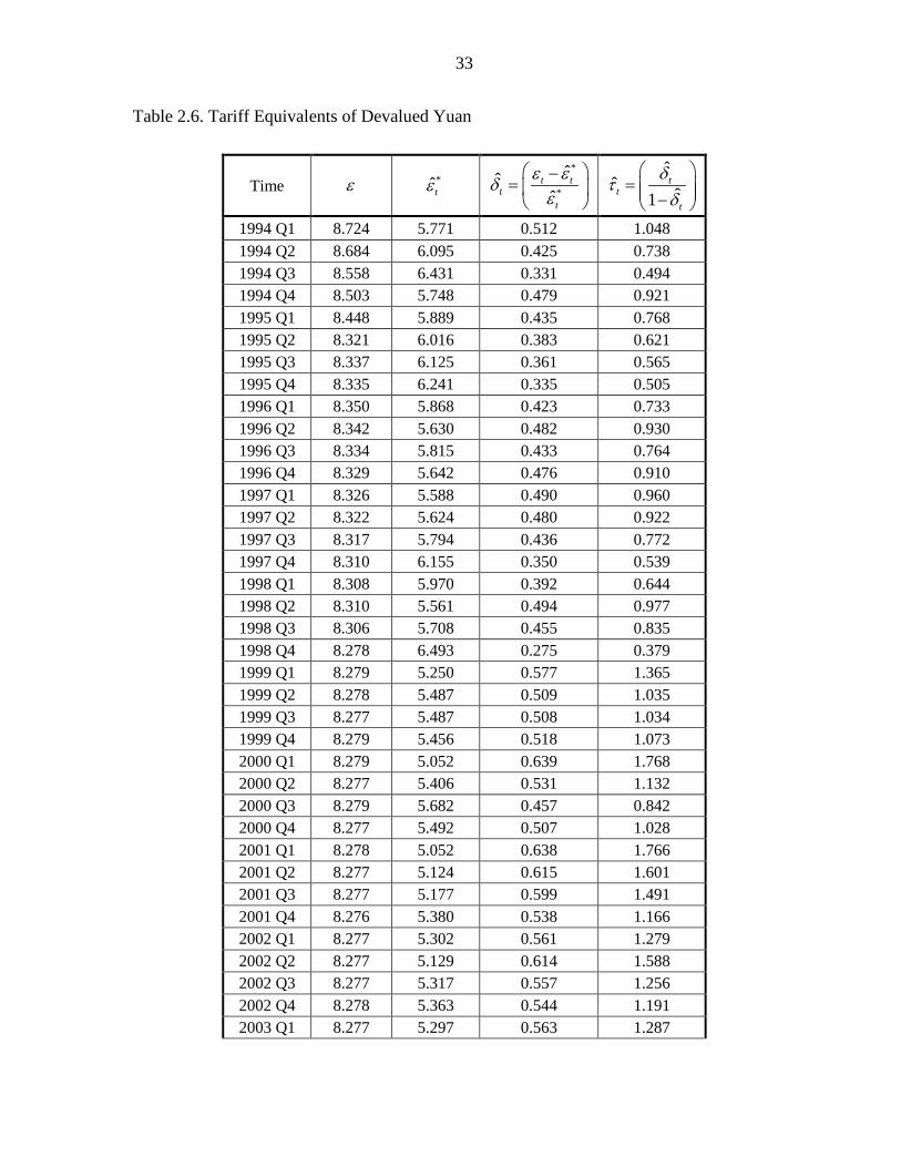
33

Table 2.6. Tariff Equivalents of Devalued Yuan

Time ε *t̂ε

*

*

ˆˆˆ

t tt

t

ε εδε

−=

ˆ

ˆ ˆ1t

tt

δτδ

= −

1994 Q1 8.724 5.771 0.512 1.048 1994 Q2 8.684 6.095 0.425 0.738 1994 Q3 8.558 6.431 0.331 0.494 1994 Q4 8.503 5.748 0.479 0.921 1995 Q1 8.448 5.889 0.435 0.768 1995 Q2 8.321 6.016 0.383 0.621 1995 Q3 8.337 6.125 0.361 0.565 1995 Q4 8.335 6.241 0.335 0.505 1996 Q1 8.350 5.868 0.423 0.733 1996 Q2 8.342 5.630 0.482 0.930 1996 Q3 8.334 5.815 0.433 0.764 1996 Q4 8.329 5.642 0.476 0.910 1997 Q1 8.326 5.588 0.490 0.960 1997 Q2 8.322 5.624 0.480 0.922 1997 Q3 8.317 5.794 0.436 0.772 1997 Q4 8.310 6.155 0.350 0.539 1998 Q1 8.308 5.970 0.392 0.644 1998 Q2 8.310 5.561 0.494 0.977 1998 Q3 8.306 5.708 0.455 0.835 1998 Q4 8.278 6.493 0.275 0.379 1999 Q1 8.279 5.250 0.577 1.365 1999 Q2 8.278 5.487 0.509 1.035 1999 Q3 8.277 5.487 0.508 1.034 1999 Q4 8.279 5.456 0.518 1.073 2000 Q1 8.279 5.052 0.639 1.768 2000 Q2 8.277 5.406 0.531 1.132 2000 Q3 8.279 5.682 0.457 0.842 2000 Q4 8.277 5.492 0.507 1.028 2001 Q1 8.278 5.052 0.638 1.766 2001 Q2 8.277 5.124 0.615 1.601 2001 Q3 8.277 5.177 0.599 1.491 2001 Q4 8.276 5.380 0.538 1.166 2002 Q1 8.277 5.302 0.561 1.279 2002 Q2 8.277 5.129 0.614 1.588 2002 Q3 8.277 5.317 0.557 1.256 2002 Q4 8.278 5.363 0.544 1.191 2003 Q1 8.277 5.297 0.563 1.287

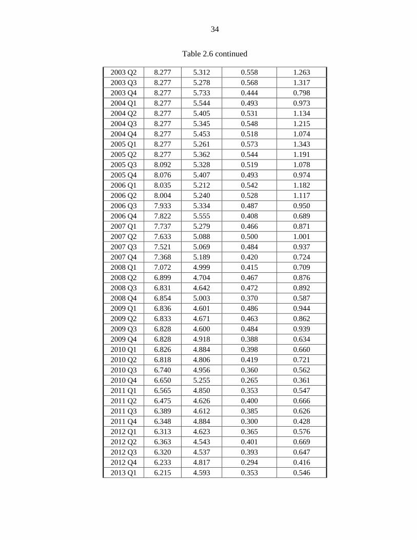
34

Table 2.6 continued

2003 Q2 8.277 5.312 0.558 1.263 2003 Q3 8.277 5.278 0.568 1.317 2003 Q4 8.277 5.733 0.444 0.798 2004 Q1 8.277 5.544 0.493 0.973 2004 Q2 8.277 5.405 0.531 1.134 2004 Q3 8.277 5.345 0.548 1.215 2004 Q4 8.277 5.453 0.518 1.074 2005 Q1 8.277 5.261 0.573 1.343 2005 Q2 8.277 5.362 0.544 1.191 2005 Q3 8.092 5.328 0.519 1.078 2005 Q4 8.076 5.407 0.493 0.974 2006 Q1 8.035 5.212 0.542 1.182 2006 Q2 8.004 5.240 0.528 1.117 2006 Q3 7.933 5.334 0.487 0.950 2006 Q4 7.822 5.555 0.408 0.689 2007 Q1 7.737 5.279 0.466 0.871 2007 Q2 7.633 5.088 0.500 1.001 2007 Q3 7.521 5.069 0.484 0.937 2007 Q4 7.368 5.189 0.420 0.724 2008 Q1 7.072 4.999 0.415 0.709 2008 Q2 6.899 4.704 0.467 0.876 2008 Q3 6.831 4.642 0.472 0.892 2008 Q4 6.854 5.003 0.370 0.587 2009 Q1 6.836 4.601 0.486 0.944 2009 Q2 6.833 4.671 0.463 0.862 2009 Q3 6.828 4.600 0.484 0.939 2009 Q4 6.828 4.918 0.388 0.634 2010 Q1 6.826 4.884 0.398 0.660 2010 Q2 6.818 4.806 0.419 0.721 2010 Q3 6.740 4.956 0.360 0.562 2010 Q4 6.650 5.255 0.265 0.361 2011 Q1 6.565 4.850 0.353 0.547 2011 Q2 6.475 4.626 0.400 0.666 2011 Q3 6.389 4.612 0.385 0.626 2011 Q4 6.348 4.884 0.300 0.428 2012 Q1 6.313 4.623 0.365 0.576 2012 Q2 6.363 4.543 0.401 0.669 2012 Q3 6.320 4.537 0.393 0.647 2012 Q4 6.233 4.817 0.294 0.416 2013 Q1 6.215 4.593 0.353 0.546

35

Table 2.6 continued

2013 Q2 6.134 4.477 0.370 0.588 2013 Q3 6.120 4.432 0.381 0.615 2013 Q4 6.074 4.989 0.217 0.278 2014 Q1 6.0509 4.588 0.319 0.468 2014 Q2 6.2246 4.329 0.438 0.779 2014 Q3 6.1984 4.389 0.412 0.702 2014 Q4 6.1251 4.874 0.257 0.345 2015 Q1 6.2181 4.645 0.339 0.512 2015 Q2 6.2010 4.485 0.382 0.619 2015 Q3 6.2085 4.494 0.381 0.617

36

CHAPTER 3. UNEMPLOYMENT AND OPTIMAL EXCHANGE RATE

IN AN OPEN ECONOMY

3.1 Abstract

China has been criticized for adopting a low yuan policy to take unfair advantage of

its trading partners. This paper considers the optimal exchange rate policy of a Keynesian

open economy with unemployed resources. In the case of Cobb-Douglas utility and

production functions, indirect utility is monotone-increasing and concave in the exchange

rate. Yuan devaluation is shown to reduce unemployment. Moreover, the optimal exchange

rate is one which guarantees full employment. The United States may want to choose a

different rate which ensures full employment. The two countries could negotiate an

intermediate exchange rate for which some unemployment exists in both countries.

3.2. Introduction

Due to its mounting currency reserves since the 1990s, China’s exchange rate policy

has been under intense scrutiny. According to the State Administration of Foreign Exchange

of People’s Bank of China (PBC), China’s foreign exchange reserve was $22 billion in 1993.

China’s foreign exchange reserve has since increased steadily, to $3.1 trillion in October

2016. Such a dramatic rise in China’s cumulative trade surplus has provoked much debate

concerning China’s currency valuation.

37

Most major currencies except the renminbi are freely floating vis-à-vis other

currencies, except the renminbi. It is argued that China may be deliberately depressing the

yuan in the hope of stimulating domestic production. In the celebrated Mundell (1963)-

Fleming(1964) model, currency devaluation influences a country’s balance of payments,

thereby affecting production and unemployment. In a study of ten countries, Gylfason and

Schmid (1983) show that devaluation has positive output effects.

In an open economy, the government may be more interested in the output effects of

currency devaluation. Helpman (1976) considered a single-period framework with a

nontraded good and showed that devaluation increases employment, while Cuddington

(1981) investigated the contemporaneous effect of devaluation. More recently, Batra and

Beladi (2013) suggest that both China and Japan kept their currency values low relative to

those of other nations such as the United States and Europe in order to maintain

unemployment below a target rate.iv Jin and Choi (2013) noted that while some profits might

be generated in the short run by slightly deviating from the equilibrium exchange rates,

excessive hoarding of reserve assets in the long run can only result in losses to PBC’s

balance of payment account. Jin et al (2016) showed that in a two-period model

nonintervention is the optimal exchange rate policy. However, the prevailing view is that

China has intentionally depressed the value of the yuan to gain unfair advantages in the

global market. (Cheung et al., 2009; Cheung, 2012)

In a developing country like China, the goal of keeping the unemployment rate low

might take precedence over other economic issues. Reducing unemployment may be the

principal motive for adopting the low yuan policy. For instance, Overholt (2010) argues that

yuan appreciation would increase China’s unemployment. Developing countries often

38

encourage trade surpluses to prepare for future contingencies. Goldstein and Lardy (2006)

suggest that China’s undervaluation of the renminbi contributed to growing trade surpluses.

Also, China wants the renminbi to be an international reserve currency, but the Chinese

government is reluctant to make the yuan fully convertible.

This paper investigates the optimal exchange rate for a Keynesian open economy.v

Open-economy macroeconomic models are predominantly based on an economy producing a

single homogeneous good.vi Frenkel and Ros (2006) developed an unemployment model in

which countries produce a nontraded good and a traded good to analyze the effect of

exchanges on unemployment. Vasylenko and Vasylenko (2005) first considered the

conditions for trade balance stabilization with two traded sectors. The present paper’s main

contribution is to analyze the effect of currency devaluation on unemployment and welfare in

an open economy which produces two tradable goods. Currency devaluation changes the

relative price of the exportable. Trade is balanced and hence no currency misalignment

occurs.vii Using the Cobb-Douglas utility and production functions, we show that under

certain conditions, the exchange rate which guarantees full employment is the optimal policy.

Section 3.2 introduces the basic two-sector, two-country model with unemployment.

Section 3.3 investigates the effect of yuan devaluation on exchange rate pass-through into the

yuan price of China’s exportable good. Section 3.4 considers the effect of yuan devaluation

on income and welfare, while Section 3.5 explores the effect on unemployment. Section 3.6

offers a numerical example to illustrate the main propositions. Section 3.7 provides

concluding remarks.

39

3.3. The Two-Sector Keynesian Model with Unemployment

In this section we consider a Keynesian open economy model with two goods to

consider China’s optimal exchange rate policy. Let China’s importable good Z be the

numéraire, i.e., its dollar price * 1=P , and let δ denote the yuan price of the dollar. Exchange

rate pass-through into the import price is perfect, viii and the yuan price of the importable is

.P An increase in δ represents an increase in the yuan price of the dollar, and hence a yuan

depreciation. We assume that the dollar price of the importable good P* is fixed in the

importing country, and its yuan price is *P P δ= , where δ is the yuan price of the dollar.

Each country is assumed to fix the price of its exportable in terms of its own

currency. That is, the yuan price of good C, which China exports, is b, while its dollar price

is denoted by *b . Likewise, the dollar price P* of good Z is fixed, equal to unity. The yuan

price of good Z is denoted by P. The relative price of good Z in China can be written as:

* * *./ *

P P P Pb b b b

δδ

= = = That is, the relative price of good Z is the same in both countries,

regardless of the exchange rate. However, a change in the exchange rate may affect the

relative price of good Z.

Assumptions

We now consider a two-sector Keynesian model of two countries producing two

goods, C and Z. Unemployment exists in both the capital and labor markets. The wage rate w

and capital rental r are assumed to be fixed in the short run. As a basis for analyzing the

effects of yuan devaluation, we employ the following assumptions:

40

(i) Two factors, capital K and labor L, are used to produce two goods, C and Z. China

is assumed to export C and import Z.ix

(ii) The dollar price of good Z is normalized, i.e., * 1.P =

(iii) The Chinese government pegs the yuan to the dollar, and the yuan price of the

importable is * .P P δ δ= =

(iv) Cobb-Douglas production functions are used in both industries.

(v) Unemployment exists in both capital and labor markets.

(vi) Consumer preferences are represented by a Cobb-Douglas utility function in both

countries.

China

China produces two goods, using two factors: capital (K) and labor (L) inputs.

Domestic outputs of the traded goods are given by 1 1( , ) ,C C C C CC F L K A L Kα β= = and

2 2( , )Z Z Z Z ZZ G L K A L Kα β= = , where jL and jK denote the amounts of labor and capital inputs

employed in sector j = C, Z. Both production functions are assumed to exhibit decreasing

returns to scale (DRS), i.e., 1 1 1,α β+ < and 2 2 1.α β+ < DRS implies that the production

functions (.)F and (.)G are monotone-increasing and concave.x

China’s Supplies of Tradable Goods

41

Since labor and capital inputs are not fully employed and are immobile

internationally, *w w≠ and *.r r≠ Let CΠ and ZΠ denote the profits of industries, C and

Z, respectively. Total profit of the Chinese economy in yuan is

1 1 2 2 ,C Z C C C Z Z Z C C Z ZbA L K PA L K wL rK wL rKα β α βΠ = Π +Π = + − − − − (31)

where b and P are the yuan prices of goods C and Z, ,iL and iK are input demands of labor

and capital in sector i = C, Z. Let L and K denote China’s labor and capital endowments.

The central planner’s problem is to choose , , ,C Z CL L K and ZK subject to

, .C Z C ZL L L K K K+ < + < Due to unemployment, a production mix of C and Z does not

occur along a production possibility frontier (PPF). The first order conditions are

1 1 1 1

2 2 2 2

1 11 1

1 12 2

, ,

, .C C C C C C

Z Z Z Z Z Z

b A L K w b A L K r

P A L K w P A L K r

α β α β

α β α β

α β

α β

− −

− −

= =

= = (32)

The input demands for labor and capital in the production of the two goods are as follows:

1 1 1 11 1 1 1

1 1 1 1

2 2 2 22 2 2 2

2 2 2 2

1/(1 ) 1/(1 )1 11 1 1 1

1 1

1/(1 ) 1/(1 )1 12 2 2 2

1 1

, ,

, .

C CC C

Z ZZ Z

b A b AL Kw r w r

P A P AL Kw r w r

α β α ββ β α α

β β α α

α β α ββ β α α

β β α α

α β α β

α β α β

− − − −− −

− −

− − − −− −

− −

= =

= =

(33)

The optimal supplies of goods, C and Z, are functions of factor prices, w and r:

1 11 1 1 11 1

1 1

2 22 2 2 22 2

2 2

1/(1 )

1 1

1/(1 )

2 2

( , ) ,

Z( , ) .

CC C C

ZZ Z Z

b AC b P A L Kw r

P Ab P A L Kw r

α βα β α βα β

α β

α βα β α βα β

α β

α β

α β

− −+

− −+

= =

= =

(34)

42

China’s Demands for Tradable Goods

The preferences of Chinese consumers are represented by a Cobb-Douglas utility

function,

1( , ) ,U c z c zγ γ−= (35)

where c and z are China’s consumption of the exportable and importable, respectively.xi

The equilibrium condition for optimal consumption is:

,c

z

U bU P

= (36)

where b and P are the yuan prices of exportable good C and importable good Z, respectively.

Thus, consumer demands for the two goods are written as: Icbγ

= and (1 ) ,IzPγ−

=

where I is China’s income in yuan. Since both factors are unemployed and the total profit is

distributed to consumers, the total income of China is

( ) ( ) .C Z C ZI w L L r K K bC PZ= + + + +Π = + The budget constraint in yuan is given by:

.bc Pz I+ = (37)

China’s national income is

1 1 2 21 1 2 2

1 1 2 2

1/(1 ) 1/(1 )

1 1 2 2 .C Zb A P AI bC PZw r w r

α β α βα β α β

α β α β

α β α β− − − −

= + = +

(38)

Suppose China lends S dollars to the United States. Then China’s expenditure in yuan

is

43

1 1 2 21 1 2 2

1 1 2 2

1/(1 ) 1/(1 )

1 1 2 2 .C Zb A P AIw r w r

α β α βα β α β

α β α β

α β α β− − − −

= +

(39)

China’s consumer demands for two tradable goods are written as:

1 1 2 22 21 1 2 21 12 2

1 1 2 2

1 1 22 21 1 2 21 12 2

1 1 2 2

11/(1 ) 1/(1 )1

11 1 2 2

11/(1 ) 1/(11

11 1 2 2

,

(1 )

C Z

C Z

A Abcb w r w r

A Abzw r w r

α β α βα βα β α βα βα β

α β α β

α β αα βα β α βα βα β

α β α β

α β α βδγ δδ

α β α βγ δδ

− − − −+− −− −

− − − −+− −− −

= +

= − +

2 )

.β

(40)

United States

The United States also is assumed to produce the two goods, using two factors,

capital (K) and labor (L) inputs. Since both inputs are unemployed, production does not occur

on the PPF. Recall that the United States and China use the same technologies in the

production of two goods, C and Z. U.S. outputs of the tradable goods are given by

1 1* ** ** ( , ) ,C C C C CC F L K A L Kα β= = and 2 2* ** ** ( , )Z Z Z Z ZZ G L K A L Kα β= = , where *jL and *

jK denote

the labor and capital inputs employed in sector j = C*, Z*.

U.S. Supplies of Tradable Goods

Let **CΠ and *

*ZΠ denote U.S. profits of industries C* and Z*. The total U.S. profit in

dollars is:

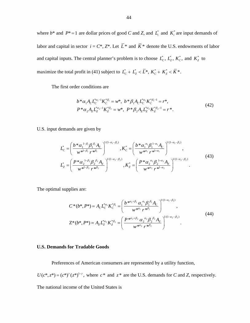
1 1 2 2* * * ** * * * * ** * * * * ** * * *( ) *( ),C Z C C C Z Z Z C Z C Zb A L K P A L K w L L r K Kα β α βΠ = Π +Π = + − + − + (41)

44

where b* and * 1P = are dollar prices of good C and Z, and *iL and *

iK are input demands of

labor and capital in sector i = C*, Z*. Let *L and *K denote the U.S. endowments of labor

and capital inputs. The central planner’s problem is to choose * * *, , ,C Z CL L K and *ZK to

maximize the total profit in (41) subject to * * * **, *.C Z C ZL L L K K K+ < + <

The first order conditions are

1 1 1 1

2 2 2 2

* 1 * * * 11 1

* 1 * * * 12 2

* *, * *,

* *, * *.C C C C C C

Z Z Z Z Z Z

b A L K w b A L K r

P A L K w P A L K r

α β α β

α β α β

α β

α β

− −

− −

= =

= = (42)

U.S. input demands are given by

1 1 1 11 1 1 1

1 1 1 1

2 2 2 22 2 2 2

2 2 2 2

1/(1 ) 1/(1 )1 1* *1 1 1 1

1 1

1/(1 ) 1/(1 )1 1* *2 2 2 2

1 1

* *, ,* * * *

* *, .* * * *

C CC C

Z ZZ Z

b A b AL Kw r w r

P A P AL Kw r w r

α β α ββ β α α

β β α α

α β α ββ β α α

β β α α

α β α β

α β α β

− − − −− −

− −

− − − −− −

− −

= =

= =

(43)

The optimal supplies are:

1 11 1 1 11 1

1 1

2 22 2 2 22 2

2 2

1/(1 )* * 1 1

1/(1 )* * 2 2

**( *, *) ,* *

*Z*( *, *) .* *

CC C C

ZZ Z Z

b AC b P A L Kw r

P Ab P A L Kw r

α βα β α βα β

α β

α βα β α βα β

α β

α β

α β

− −+

− −+

= =

= =

(44)

U.S. Demands for Tradable Goods

Preferences of American consumers are represented by a utility function,

1( *, *) ( *) ( *) ,U c z c zγ γ−= where *c and *z are the U.S. demands for C and Z, respectively.

The national income of the United States is

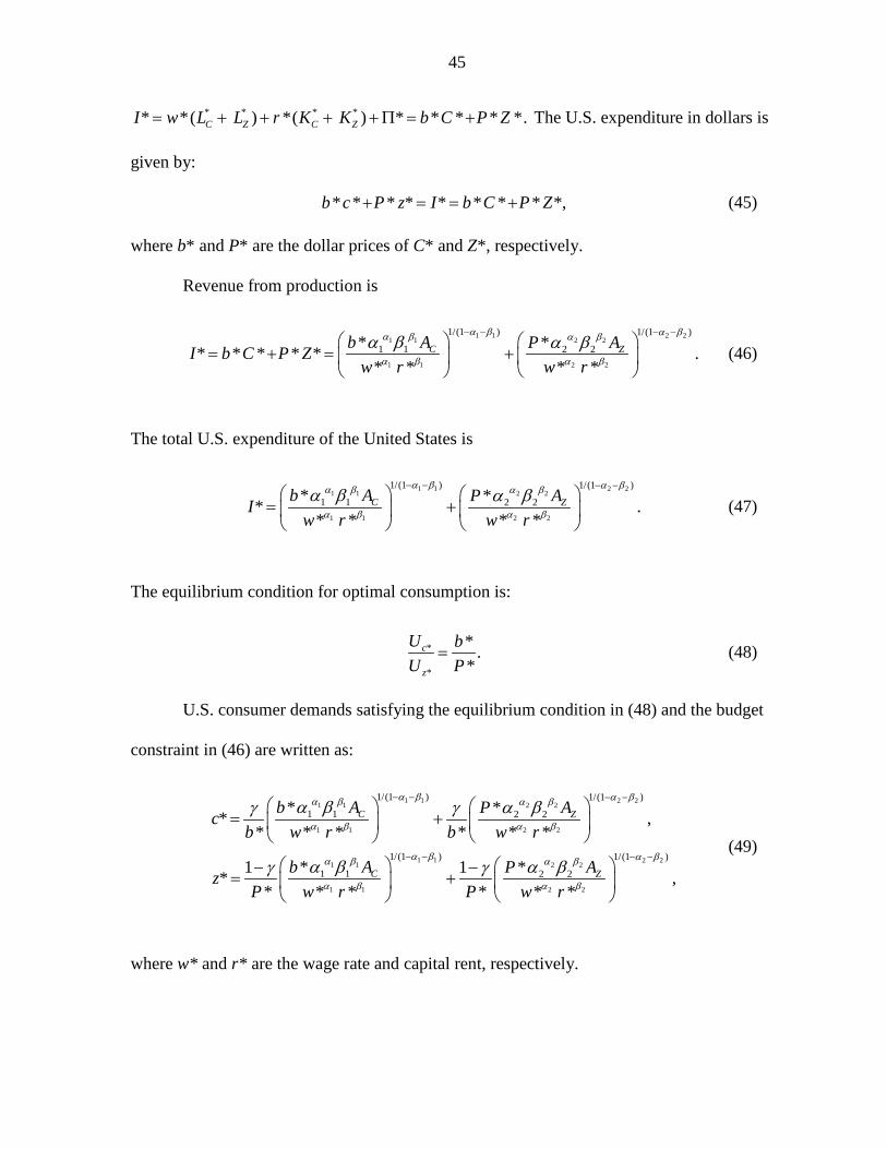
45

* * * ** *( ) *( ) * * * * *.C Z C ZI w L L r K K b C P Z= + + + +Π = + The U.S. expenditure in dollars is

given by:

* * * * * * * * *,b c P z I b C P Z+ = = + (45)

where b* and P* are the dollar prices of C* and Z*, respectively.

Revenue from production is

1 1 2 21 1 2 2

1 1 2 2

1/(1 ) 1/(1 )

1 1 2 2* ** * * * * .* * * *

C Zb A P AI b C P Zw r w r

α β α βα β α β

α β α β

α β α β− − − −

= + = +

(46)

The total U.S. expenditure of the United States is

1 1 2 21 1 2 2

1 1 2 2

1/(1 ) 1/(1 )

1 1 2 2* ** .* * * *

C Zb A P AIw r w r

α β α βα β α β

α β α β

α β α β− − − −

= +

(47)

The equilibrium condition for optimal consumption is:

*

*

* .*

c

z

U bU P

= (48)

U.S. consumer demands satisfying the equilibrium condition in (48) and the budget

constraint in (46) are written as:

1 1 2 21 1 2 2

1 1 2 2

1 1 2 21 1 2 2

1 1 2 2

1/(1 ) 1/(1 )

1 1 2 2

1/(1 ) 1/(1 )

1 1 2 2

* ** ,* * * * * *

* *1 1* ,* * * * * *

C Z

C Z

b A P Acb w r b w r

b A P AzP w r P w r

α β α βα β α β

α β α β

α β α βα β α β

α β α β

α β α βγ γ

α β α βγ γ

− − − −

− − − −

= +

− −= +

(49)

where w* and r* are the wage rate and capital rent, respectively.

46

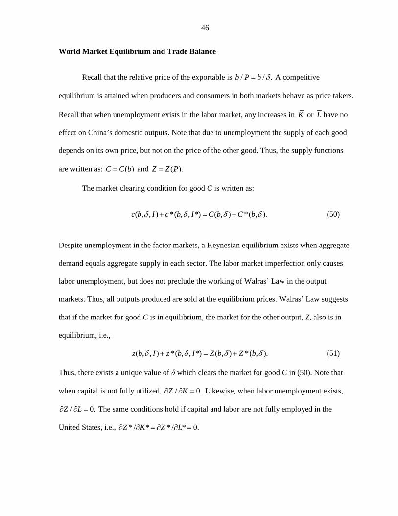
World Market Equilibrium and Trade Balance

Recall that the relative price of the exportable is / / .b P b δ= A competitive

equilibrium is attained when producers and consumers in both markets behave as price takers.

Recall that when unemployment exists in the labor market, any increases in K or L have no

effect on China’s domestic outputs. Note that due to unemployment the supply of each good

depends on its own price, but not on the price of the other good. Thus, the supply functions

are written as: ( )C C b= and ( ).Z Z P=

The market clearing condition for good C is written as:

( , , ) *( , , *) ( , ) *( , ).c b I c b I C b C bδ δ δ δ+ = + (50)

Despite unemployment in the factor markets, a Keynesian equilibrium exists when aggregate

demand equals aggregate supply in each sector. The labor market imperfection only causes

labor unemployment, but does not preclude the working of Walras’ Law in the output

markets. Thus, all outputs produced are sold at the equilibrium prices. Walras’ Law suggests

that if the market for good C is in equilibrium, the market for the other output, Z, also is in

equilibrium, i.e.,

( , , ) *( , , *) ( , ) *( , ).b I z b I Z b Z bz δ δ δ δ+ = + (51)

Thus, there exists a unique value of δ which clears the market for good C in (50). Note that

when capital is not fully utilized, / 0Z K∂ ∂ = . Likewise, when labor unemployment exists,

/ 0.Z L∂ ∂ = The same conditions hold if capital and labor are not fully employed in the

United States, i.e., * / * * / * 0.Z K Z L∂ ∂ = ∂ ∂ =

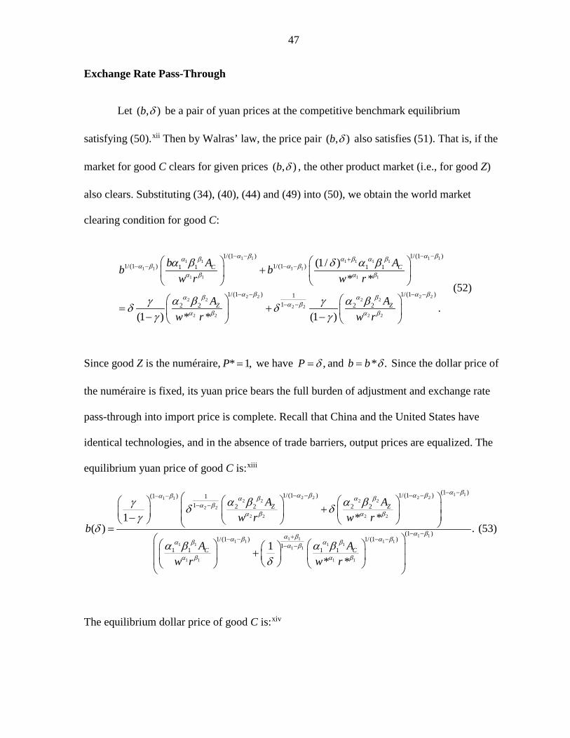
47

Exchange Rate Pass-Through

Let ( , )b δ be a pair of yuan prices at the competitive benchmark equilibrium

satisfying (50).xii Then by Walras’ law, the price pair ( , )b δ also satisfies (51). That is, if the

market for good C clears for given prices ( , )b δ , the other product market (i.e., for good Z)

also clears. Substituting (34), (40), (44) and (49) into (50), we obtain the world market

clearing condition for good C:

1 1 1 11 1 1 1 1 11 1 1 1

1 1 1 1

2 2 2 22 2 2 22 2

2 2 2 2

1/(1 ) 1/(1 )1/(1 ) 1/(1 )1 1 1 1

1/(1 ) 1/(1 )112 2 2 2

(1/ )* *

.(1 ) * * (1 )

C C

Z Z

b A Ab bw r w r

A Aw r w r

α β α βα β α β α βα β α β

α β α β

α β α βα β α βα β

α β α β

α β δ α β

α β α βγ γδ δγ γ

− − − −+− − − −

− − − −

− −

+

= + − −

(52)

Since good Z is the numéraire, * 1,P = we have ,P δ= and * .b b δ= Since the dollar price of

the numéraire is fixed, its yuan price bears the full burden of adjustment and exchange rate

pass-through into import price is complete. Recall that China and the United States have

identical technologies, and in the absence of trade barriers, output prices are equalized. The

equilibrium yuan price of good C is:xiii

1 12 2 2 21 1 2 2 2 22 2

2 2 2 2

1 11 11 1 1 11 1

1 1 1 1

(1 )1/(1 ) 1/(1 )(1 ) 11 2 2 2 2

1/(1 ) 1/1

1 1 1 1

1 * *( )

1* *

Z Z

C C

A Aw r w r

bA A

w r w r

α βα β α βα β α β α βα β

α β α β

α βα βα β α βα β

α β α β

α β α βγ δ δγ

δα β α β

δ

− −− − − −− −− −

+− −− −

+ − = +

1 11 1

(1 )(1 )

.α βα β

− −− −

(53)

The equilibrium dollar price of good C is:xiv

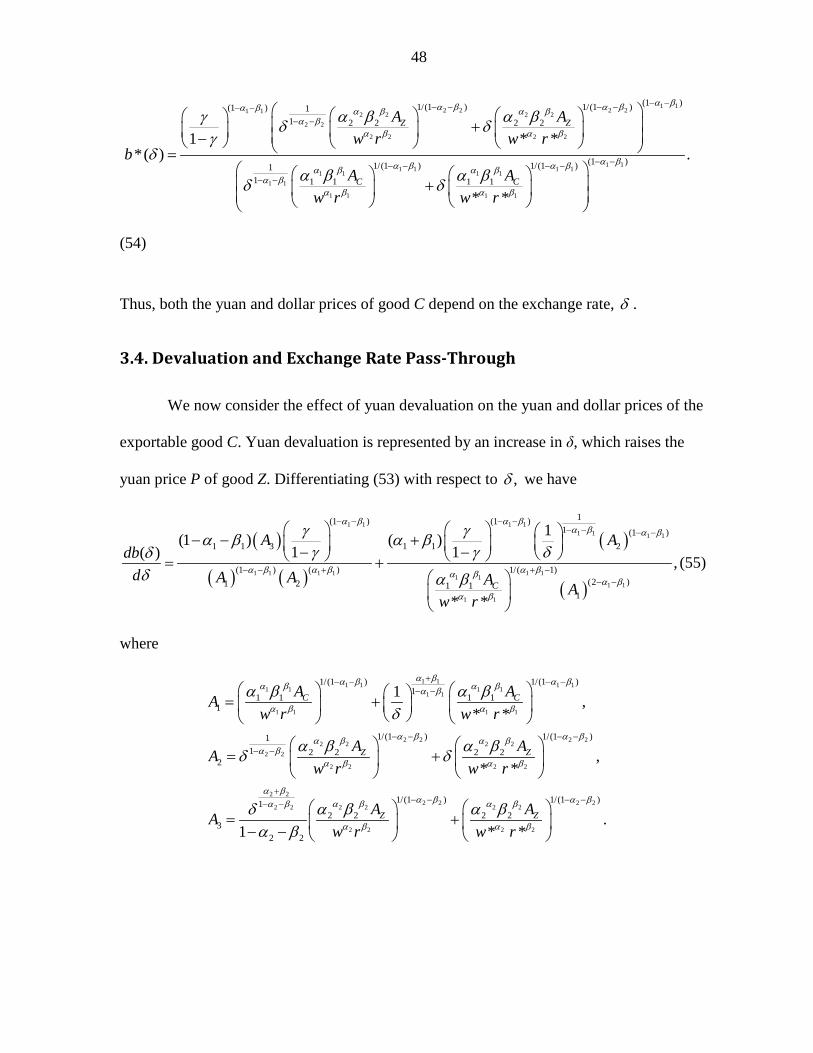
48

1 12 2 2 21 1 2 2 2 22 2

2 2 2 2

1 1 1 11 1 1 11 1

1 1 1 1

(1 )1/(1 ) 1/(1 )(1 ) 11 2 2 2 2

1/(1 ) 1/(1 )11 1 1 1 1

1 * **( )

* *

Z Z

C C

A Aw r w r

bA A

w r w r

α βα β α βα β α β α βα β

α β α β

α β α βα β α βα β

α β α β

α β α βγ δ δγ

δα β α βδ δ

− −− − − −− −− −

− − − −

− −

+ − =

+

1 1(1 ) .α β− −

(54)

Thus, both the yuan and dollar prices of good C depend on the exchange rate, δ .

3.4. Devaluation and Exchange Rate Pass-Through

We now consider the effect of yuan devaluation on the yuan and dollar prices of the

exportable good C. Yuan devaluation is represented by an increase in δ, which raises the

yuan price P of good Z. Differentiating (53) with respect to ,δ we have

( )

( ) ( )

( )

( )

1 1 1 11 1 1 1

1 1 1 1 1 11 11 1

1 1

1(1 ) (1 )1 (1 )

1 1 3 1 1 2

(1 ) ( ) 1/( 1)(2 )1 2 1 1

1

1(1 ) ( )1 1( ) ,

* *C

A Adb

d A A A Aw r

α β α βα β α β

α β α β α βα βα β

α β

γ γα β α βγ γ δδ

δ α β

− − − −− − − −

− − + + −− −

− − + − − = +

(55)

where

1 11 1 1 11 1 1 11 1

1 1 1 1

2 2 2 22 2 2 22 2

2 2 2 2

2 2

2 2

1/(1 ) 1/(1 )1

1 1 1 11

1/(1 ) 1/(1 )11 2 2 2 2

2

1

32 2

1 ,* *

,* *

1

C C

Z Z

A AAw r w r

A AAw r w r

A

α βα β α βα β α βα β

α β α β

α β α βα β α βα β

α β α β

α βα β

α β α βδ

α β α βδ δ

αδα β

+− − − −− −

− − − −

− −

+− −

= +

= +

=− −

2 2 2 22 2 2 2

2 2 2 2

1/(1 ) 1/(1 )

2 2 2 2 .* *

Z ZA Aw r w r

α β α βα β α β

α β α β

β α β− − − −

+

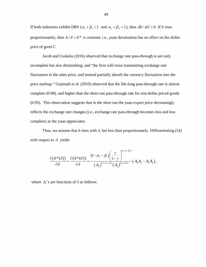
49

If both industries exhibit DRS ( 1 1 1α β+ < and 2 2 1α β+ < ), then / 0.db dδ > If b rises

proportionately, then / *b bδ = is constant; i.e., yuan devaluation has no effect on the dollar

price of good C.

Jacob and Uusküla (2016) observed that exchange rate pass-through is not only

incomplete but also diminishing, and “the firm will resist transmitting exchange rate

fluctuation to the sales price, and instead partially absorb the currency fluctuation into the

price markup.” Gopinath et al. (2010) observed that the life-long pass-through rate is almost

complete (0.98), and higher than the short-run pass-through rate for non-dollar priced goods

(0.95). This observation suggests that in the short run the yuan export price decreasingly

reflects the exchange rate changes (i.e., exchange rate pass-through becomes less and less

complete) as the yuan appreciates.

Thus, we assume that b rises with δ, but less than proportionately. Differentiating (54)

with respect to δ yields

( ) ( )( ) ( )

( )

1 1

1 1 1 1

(1 )

1 1

0 3 2 4(2 ) ( )0 2

(1 )*( ) *( ) 1 ,

b bA A A A

A A

α β

α β α β

γα βδ δ γ

δ δ

− −

− − +

− − ∂ ∂ − = = −

∂ ∂

where iA ’s are functions of δ as follows:

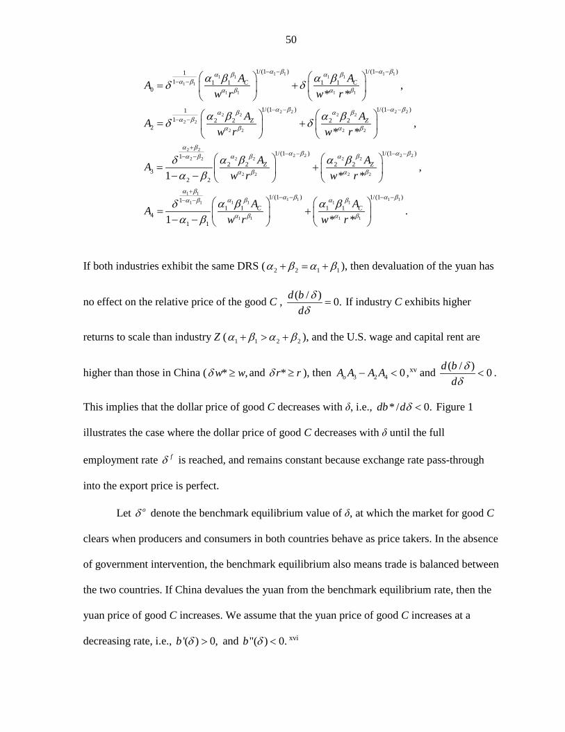
50

1 1 1 11 1 1 11 1

1 1 1 1

2 2 2 22 2 2 22 2

2 2 2 2

2 2

2 22 2

1/(1 ) 1/(1 )11 1 1 1 1

0

1/(1 ) 1/(1 )11 2 2 2 2

2

12 2

32 2

,* *

,* *

1

C C

Z Z

Z

A AAw r w r

A AAw r w r

AAw

α β α βα β α βα β

α β α β

α β α βα β α βα β

α β α β

α βα βα β

α β α βδ δ

α β α βδ δ

α βδα β

− − − −

− −

− − − −

− −

+− −

= +

= +

=− −

2 2 2 22 2

2 2 2 2

1 11 1 1 11 1 1 11 1

1 1 1 1

1/(1 ) 1/(1 )

2 2

1/(1 ) 1/(1 )11 1 1 1

41 1

,* *

.1 * *

Z

C C

Ar w r

A AAw r w r

α β α βα β

α β α β

α βα β α βα β α βα β

α β α β

α β

α β α βδα β

− − − −

+− − − −− −

+

= + − −

If both industries exhibit the same DRS ( 2 2 1 1α β α β+ = + ), then devaluation of the yuan has

no effect on the relative price of the good C , ( / ) 0.d bd

δδ

= If industry C exhibits higher

returns to scale than industry Z ( 1 1 2 2α β α β+ > + ), and the U.S. wage and capital rent are

higher than those in China ( * ,w wδ ≥ and *r rδ ≥ ), then 3 2 4 0oA A A A− < ,xv and ( / ) 0d bd

δδ

< .

This implies that the dollar price of good C decreases with δ, i.e., * / 0.db dδ < Figure 1

illustrates the case where the dollar price of good C decreases with δ until the full

employment rate fδ is reached, and remains constant because exchange rate pass-through

into the export price is perfect.

Let oδ denote the benchmark equilibrium value of δ, at which the market for good C

clears when producers and consumers in both countries behave as price takers. In the absence

of government intervention, the benchmark equilibrium also means trade is balanced between

the two countries. If China devalues the yuan from the benchmark equilibrium rate, then the

yuan price of good C increases. We assume that the yuan price of good C increases at a

decreasing rate, i.e., '( ) 0,b δ > and "( ) 0.b δ < xvi

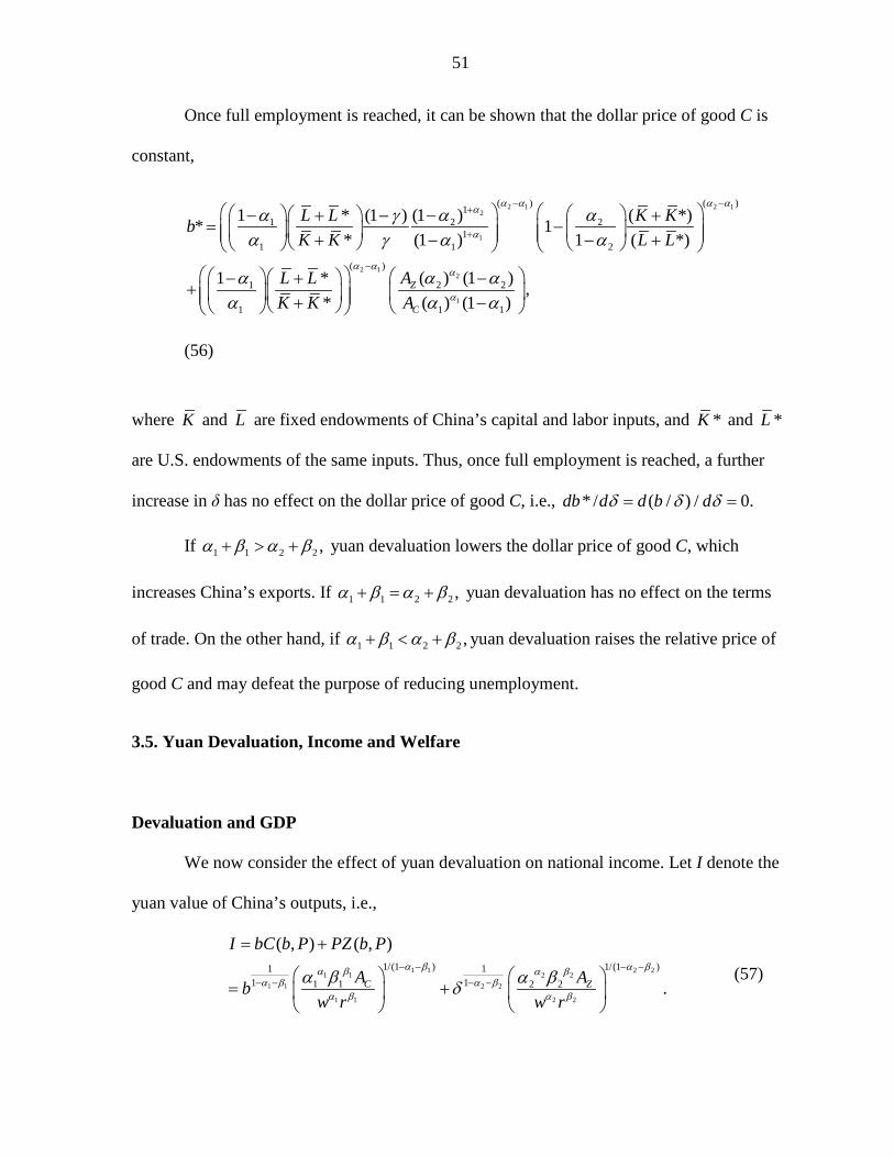
51

Once full employment is reached, it can be shown that the dollar price of good C is

constant,

2 1 2 12

1

2 12

1

( ) ( )11 2 2

11 1 2

( )

1 2 2

1 1 1

1 (1 )* (1 ) ( *)* 1* (1 ) 1 ( *)

1 ( ) (1 )* ,* ( ) (1 )

Z

C

L L K KbK K L L

AL LK K A

α α α αα

α

α α α

α

α α αγα γ α α

α α αα α α

− −+

+

−

− −+ − += − + − − +

− −++ + −

(56)

where K and L are fixed endowments of China’s capital and labor inputs, and *K and *L

are U.S. endowments of the same inputs. Thus, once full employment is reached, a further

increase in δ has no effect on the dollar price of good C, i.e., * / ( / ) / 0.db d d b dδ δ δ= =

If 1 1 2 2 ,α β α β+ > + yuan devaluation lowers the dollar price of good C, which

increases China’s exports. If 1 1 2 2 ,α β α β+ = + yuan devaluation has no effect on the terms

of trade. On the other hand, if 1 1 2 2 ,α β α β+ < + yuan devaluation raises the relative price of

good C and may defeat the purpose of reducing unemployment.

3.5. Yuan Devaluation, Income and Welfare

Devaluation and GDP

We now consider the effect of yuan devaluation on national income. Let I denote the

yuan value of China’s outputs, i.e.,

1 1 2 21 1 2 21 1 2 2

1 1 2 2

1/(1 ) 1/(1 )1 11 11 1 2 2

( , ) ( , )

.C Z

I bC b P PZ b P

A Abw r w r

α β α βα β α βα β α β

α β α β

α β α βδ− − − −

− − − −

= +

= +

(57)

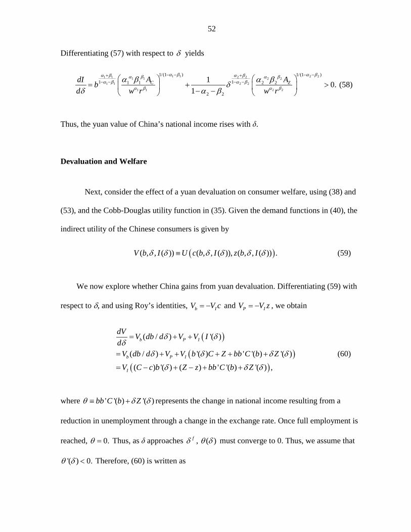
52

Differentiating (57) with respect to δ yields

1 1 2 21 1 2 21 1 2 2

1 1 2 2

1 1 2 2

1/(1 ) 1/(1 )1 11 1 2 2

2 2

1 0.1

C ZA AdI bd w r w r

α β α βα β α βα β α βα β α β

α β α β

α β α βδδ α β

− − − −+ +− − − −

= + > − − (58)

Thus, the yuan value of China’s national income rises with δ.

Devaluation and Welfare

Next, consider the effect of a yuan devaluation on consumer welfare, using (38) and

(53), and the Cobb-Douglas utility function in (35). Given the demand functions in (40), the

indirect utility of the Chinese consumers is given by

( )( , , ( )) ( , , ( )), ( , , ( )) .V b I U c b I z b Iδ δ δ δ δ δ≡ (59)

We now explore whether China gains from yuan devaluation. Differentiating (59) with

respect to δ, and using Roy’s identities, b IV V c= − and P IV V z= − , we obtain

( )

( )( )

( / ) '( )

( / ) '( ) ' '( ) '( )

( ) '( ) ( ) ' '( ) '( ) ,

b P I

b P I

I

dV V db d V V Id

V db d V V b C Z bb C b Z

V C c b Z z bb C b Z

δ δδ

δ δ δ δ

δ δ δ

= + +

= + + + + +

= − + − + +

(60)

where ' '( ) '( )bb C b Zθ δ δ≡ + represents the change in national income resulting from a

reduction in unemployment through a change in the exchange rate. Once full employment is

reached, 0.θ = Thus, as δ approaches fδ , ( )θ δ must converge to 0. Thus, we assume that

'( ) 0.θ δ < Therefore, (60) is written as

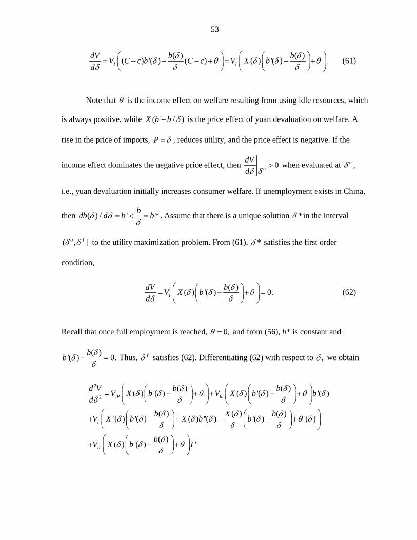
53

( ) ( )( ) '( ) ( ) ( ) '( ) .I IdV b bV C c b C c V X bd

δ δδ θ δ δ θδ δ δ

= − − − + = − + (61)

Note that θ is the income effect on welfare resulting from using idle resources, which

is always positive, while ( ' / )X b b δ− is the price effect of yuan devaluation on welfare. A

rise in the price of imports, P δ= , reduces utility, and the price effect is negative. If the

income effect dominates the negative price effect, then 0odVd δδ

> when evaluated at oδ ,

i.e., yuan devaluation initially increases consumer welfare. If unemployment exists in China,

then ( ) / ' *bdb d b bδ δδ

= < = . Assume that there is a unique solution *δ in the interval

( , ]o fδ δ to the utility maximization problem. From (61), *δ satisfies the first order

condition,

( )( ) '( ) 0.IdV bV X bd

δδ δ θδ δ

= − + = (62)

Recall that once full employment is reached, 0,θ = and from (56), b* is constant and

( )'( ) 0.bb δδδ

− = Thus, fδ satisfies (62). Differentiating (62) with respect to ,δ we obtain

2

2

( ) ( )( ) '( ) ( ) '( ) '( )

( ) ( ) ( )'( ) '( ) ( ) ''( ) '( ) '( )

( )( ) '( ) '

IP Ib

I

II

d V b bV X b V X b bd

b X bV X b X b b

bV X b I

δ δδ δ θ δ δ θ δδ δ δ

δ δ δδ δ δ δ δ θ δδ δ δ

δδ δ θδ

= − + + − + + − + − − + + − +

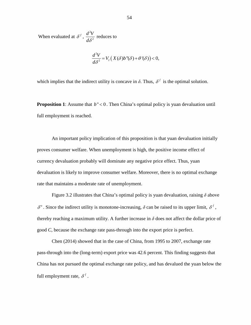
54

When evaluated at fδ , 2

2

d Vdδ

reduces to

( )2

2 ( ) ''( ) '( ) 0,Id V V X bd

δ δ θ δδ

= + <

which implies that the indirect utility is concave in δ. Thus, fδ is the optimal solution.

Proposition 1: Assume that " 0b < . Then China’s optimal policy is yuan devaluation until

full employment is reached.

An important policy implication of this proposition is that yuan devaluation initially

proves consumer welfare. When unemployment is high, the positive income effect of

currency devaluation probably will dominate any negative price effect. Thus, yuan

devaluation is likely to improve consumer welfare. Moreover, there is no optimal exchange

rate that maintains a moderate rate of unemployment.

Figure 3.2 illustrates that China’s optimal policy is yuan devaluation, raising δ above

oδ . Since the indirect utility is monotone-increasing, δ can be raised to its upper limit, fδ ,

thereby reaching a maximum utility. A further increase in δ does not affect the dollar price of

good C, because the exchange rate pass-through into the export price is perfect.

Chen (2014) showed that in the case of China, from 1995 to 2007, exchange rate

pass-through into the (long-term) export price was 42.6 percent. This finding suggests that

China has not pursued the optimal exchange rate policy, and has devalued the yuan below the

full employment rate, fδ .

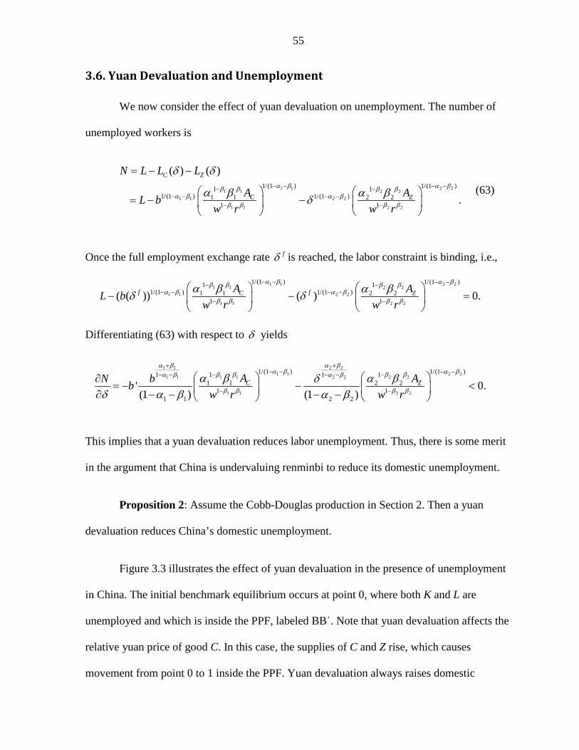
55

3.6. Yuan Devaluation and Unemployment

We now consider the effect of yuan devaluation on unemployment. The number of

unemployed workers is

1 1 2 21 1 2 21 1 2 2

1 1 2 2

1/(1 ) 1/(1 )1 11/(1 ) 1/(1 )1 1 2 2

1 1

( ) ( )

.

C Z

C Z

N L L L

A AL bw r w r

α β α ββ β β βα β α β

β β β β

δ δ

α β α βδ− − − −− −

− − − −− −

= − −

= − −

(63)

Once the full employment exchange rate fδ is reached, the labor constraint is binding, i.e.,

1 1 2 21 1 2 2

1 1 2 2

1 1 2 2

1/(1 ) 1/(1 )1 11/(1 ) 1/(1 )1 1 2 2

1 1( ( )) ( ) 0.f fC ZA AL bw r w r

α β α ββ β β βα β α β

β β β β

α β α βδ δ− − − −− −

− − − −− −

− − =

Differentiating (63) with respect to δ yields

1 1 2 21 1 2 21 1 2 21 1 2 2

1 1 2 2

1/(1 ) 1/(1 )1 11 11 1 2 2

1 11 1 2 2

' 0.(1 ) (1 )

C ZA AN bbw r w r

α β α βα β α ββ β β βα β α β

β β β β

α β α βδδ α β α β

+ +− − − −− −− − − −

− −

∂= − − < ∂ − − − −

This implies that a yuan devaluation reduces labor unemployment. Thus, there is some merit

in the argument that China is undervaluing renminbi to reduce its domestic unemployment.

Proposition 2: Assume the Cobb-Douglas production in Section 2. Then a yuan

devaluation reduces China’s domestic unemployment.

Figure 3.3 illustrates the effect of yuan devaluation in the presence of unemployment

in China. The initial benchmark equilibrium occurs at point 0, where both K and L are

unemployed and which is inside the PPF, labeled BBˈ. Note that yuan devaluation affects the

relative yuan price of good C. In this case, the supplies of C and Z rise, which causes

movement from point 0 to 1 inside the PPF. Yuan devaluation always raises domestic

56

production of both goods in so far as unemployment exists. Thus, China’s optimal policy is

to choose δ to eliminate unemployment until production occurs at point 2 along the PPF, i.e.,

.( )

f

fb bδ δ

δ=

Consider an alternative scenario in which capital is fully utilized at point 0, but

unemployment exists in the labor market. Note that the supply of good Z increases with δ.

An increase in δ not only raises the yuan price of good C, but also raises the shadow price of

capital. The latter effect partly offsets the former effect. Thus, the supply response of good C

is likely to be less pronounced than when unemployment exists in both factor markets.xvii

3.7. Numerical Example

Since there is no tariff, the yuan price of the importable is * .P P δ δ= = The price of

the exportable good C is b and its dollar price of good C is *.b

China and the United States

The United States and China are assumed to have identical production functions for

the traded goods, C and Z: .45 .15( , ) 1.3C F L K L K= = and .3 .1( , ) .Z G L K L K= = Assume that

factor prices in China are: .7w = and 1r = , and in the Unites States: * 1w = and * 0.7r = .

Labor and capital endowments are 4L = and 1K = in China and * 1L = and * 3K = in the

United States. Direct utility functions of the Chinese and U.S. consumers are represented by

.4( , ) ( )u c z cz= and .4( *, *) ( * *) .u c z c z=

From the world market clearing condition in equation (54), we obtain the optimal

yuan and dollar prices of good C:

57

( )

( )

0.41.67

1.5

0.41.67

1.5

0.396 0.446( ) ,0.575 0.44 1/

( ) 1 0.396 0.446*( ) .0.575 0.44 1/

b

bbP

δ δδδ

δ δ δδδ δ

+= +

+= =

+

Thus, as δ increases, the dollar price of good C , *( ),b δ decreases.

China’s consumer demands for the two tradable goods are written as:

( )

( )

0.41.67

1.671.5

0.41.67

1.671.5

0.396 0.4460.446 0.575 ,0.575 0.44 1/

0.39

0.4

0.4 6 0.4460.446 0.575 .0.575 0.44 1/

c

bz

b

c

δ δδδ

δ δδ δ

δδ

+= +

+

+= = +

+

China’s consumer welfare is measured by the indirect utility,

( )

.4

0.41.67

1.671.

0.8

0.4 0.4 5

( , , ( )) ( )

0.396 0.4460.446 0.575 .0.575 0

0.4

.4

481/

V b I c

b

zδ δ

δ δδδδ

=

++

+

=

(64)

We now determine whether China gains from a yuan devaluation. Mathematica was

used to generate Figure 4, which shows the impacts of yuan devaluation on the yuan and

dollar prices of good C, national income, indirect utility, and labor and capital

unemployment. When 2.44δ ≈ , both capital and labor inputs are fully utilized and

maximum utility is attained. Until fδ is reached, the exchange rate pass-through into the

yuan price is imperfect, i.e., ' / .b b δ< Once fδ is reached, a further increase in δ does not

affect the dollar price of good C, *.b

58

3.8. Concluding Remarks

This paper investigates the optimal exchange rate policy for a two-sector, Keynesian

open economy. A Cobb-Douglas utility function is used to investigate China’s optimal

exchange rate policy. In the plausible scenario where capital rents are equalized ( *)r rδ= ,

China’s wage is lower than the U.S. wage ( *)w wδ< , and industry C exhibits higher returns

to scale than industry Z ( 1 1 2 2α β α β+ > + ) , then the indirect utility function is monotone-

increasing and concave in δ, which guarantees the existence of an optimal exchange rate.

China has been widely criticized for keeping the yuan low in order to take advantage

of its trading partners. However, this paper suggests that instead China may have pursued the

low yuan policy to reduce domestic unemployment. In the case of the Cobb-Douglas utility

function, China’s optimal exchange rate is that rate which guarantees full employment. Such

a policy cannot be criticized as deliberately devaluing the yuan to take unfair advantage of

China’s trading partners. China may be preoccupied with reducing domestic unemployment.

This paper demonstrates that yuan devaluation reduces unemployment. Given the

diminishing exchange rate pass-through into export price ( "( ) 0b δ < ), China’s optimal

exchange rate is that rate which yields full employment. The model is limited in scope as it

assumes a balance of trade between two trading countries, and does not explicitly consider

trade imbalance.

Given the plausible assumption of a concave indirect utility function in the exchange rate, the

paper also shows that there is no optimal exchange rate that allows some unemployment.

From the U.S. perspective, there exists another exchange rate *δ that guarantees full

employment in the United States. This rate is lower than the rate fδ that guarantees full

59

employment in China. Instead of permitting the trading partner to set its own optimal

exchange rate, the two countries could negotiate an intermediate exchange rate, which lies

somewhere between the two optimal exchange rates, *δ and .fδ To date, the United States

has permitted China to choose its optimal rate, .fδ

60

3.9. References

Al-Abri, Almukhtar Saif, “Optimal exchange rate policy for a small oil-exporting country: A

dynamic general equilibrium perspective,” Economic Modelling 36 (2014), 88-98.

Batra, Ravi and Hamid Beladi, “The US Trade Deficit and the Rate of Interest,” Review of

International Economics 21 (2013), 614-626.

Beladi, Hamid and Reza Oladi, “On Offshoring and Trade Deficit,” Review of Development

Economics 18 (2014), 517-23.

Bruno, Michael, “The Two-Sector Open Economy and the Real Exchange Rate,” American

Economic Review 66 (1976), 566-577.

Chen, Jiatao, “Empirical research on effect of exchange rate pass-through into China’s export

price,” Bio Technology An Indian Journal 10 (2014), 1714-1720.

Cheung, Yin-Wong, “Exchange Rate Misalignment –The Case of the Chinese Renminbi,”

Handbook of Exchange Rates, Jessica James, Ian W. Marsh and Lucio Sarno (eds.),

2012.

Cheung, Yin-Wong, Menzie D. Chinn, and Eiji Fujii, “China's Current Account and

Exchange Rate,” NBER Working Paper No. 14673, 2009.

Cuddington, John, “Import Substitution Policies: A Two-Sector, Fix-Price Model,” Review of

Economic Studies 48 (1981), 327-342.

Devereux, M. B., “How does a devaluation affect the current account?,” Journal of

International Money and Finance 19 (2000), 833-851.

Fleming, J. Marcus, "Domestic financial policies under fixed and floating exchange

Rates." IMF Staff Papers 9 (1962), 369–379.

Frenkel, Roberto and Jaime Ros, “Unemployment and the Real Exchange Rate in Latin

America,” World Development 34 (2006), 631-646.

Goldstein, Morris and Nicholas Lardy, “China’s Exchange Rate Policy Dilemma,” American

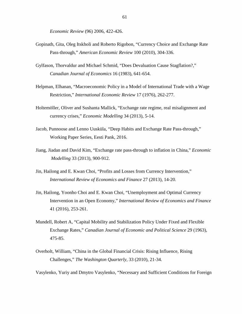
61

Economic Review (96) 2006, 422-426.

Gopinath, Gita, Oleg Itskholi and Roberto Rigobon, “Currency Choice and Exchange Rate

Pass-through,” American Economic Review 100 (2010), 304-336.

Gylfason, Thorvaldur and Michael Schmid, “Does Devaluation Cause Stagflation?,”

Canadian Journal of Economics 16 (1983), 641-654.

Helpman, Elhanan, “Macroeconomic Policy in a Model of International Trade with a Wage

Restriction,” International Economic Review 17 (1976), 262-277.

Holtemöller, Oliver and Sushanta Mallick, “Exchange rate regime, real misalignment and

currency crises,” Economic Modelling 34 (2013), 5-14.

Jacob, Punnoose and Lenno Uusküla, “Deep Habits and Exchange Rate Pass-through,”

Working Paper Series, Eesti Pank, 2016.

Jiang, Jiadan and David Kim, “Exchange rate pass-through to inflation in China,” Economic

Modelling 33 (2013), 900-912.

Jin, Hailong and E. Kwan Choi, “Profits and Losses from Currency Intervention,”

International Review of Economics and Finance 27 (2013), 14-20.

Jin, Hailong, Yoonho Choi and E. Kwan Choi, “Unemployment and Optimal Currency

Intervention in an Open Economy,” International Review of Economics and Finance

41 (2016), 253-261.

Mundell, Robert A, “Capital Mobility and Stabilization Policy Under Fixed and Flexible

Exchange Rates,” Canadian Journal of Economic and Political Science 29 (1963),

475-85.

Overholt, William, “China in the Global Financial Crisis: Rising Influence, Rising

Challenges,” The Washington Quarterly, 33 (2010), 21-34.

Vasylenko, Yuriy and Dmytro Vasylenko, “Necessary and Sufficient Conditions for Foreign

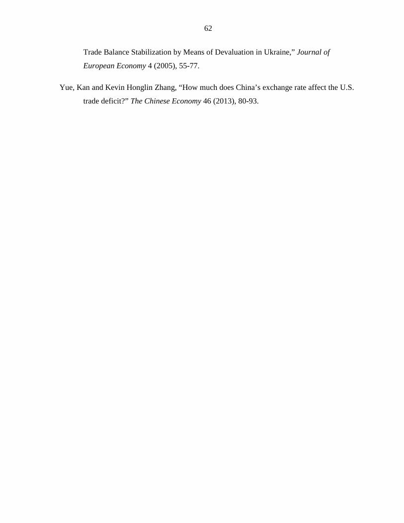
62

Trade Balance Stabilization by Means of Devaluation in Ukraine,” Journal of

European Economy 4 (2005), 55-77.

Yue, Kan and Kevin Honglin Zhang, “How much does China’s exchange rate affect the U.S.

trade deficit?” The Chinese Economy 46 (2013), 80-93.

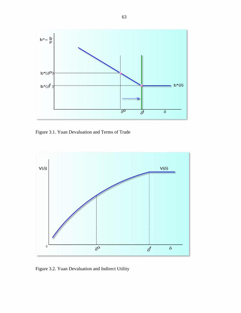
63

Figure 3.1. Yuan Devaluation and Terms of Trade

Figure 3.2. Yuan Devaluation and Indirect Utility

64

Figure 3.3. Yuan Devaluation and Output Effects

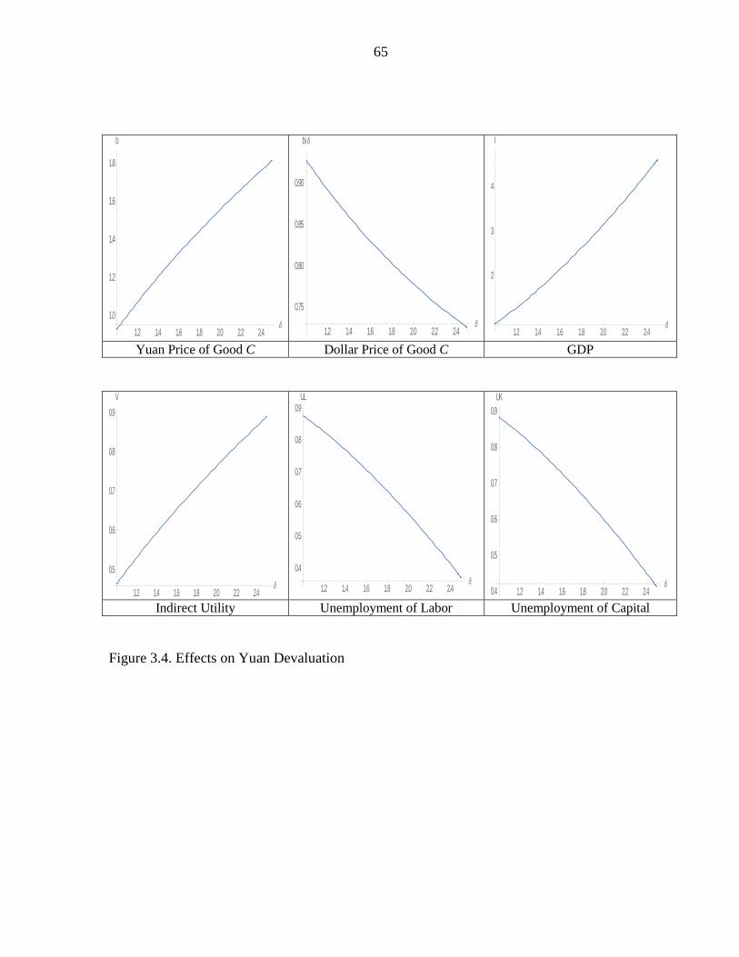
65

1.2 1.4 1.6 1.8 2.0 2.2 2.41.0

1.2

1.4

1.6

1.8

b

1.2 1.4 1.6 1.8 2.0 2.2 2.4

0.75

0.80

0.85

0.90

b

1.2 1.4 1.6 1.8 2.0 2.2 2.4

2

3

4

I

Yuan Price of Good C Dollar Price of Good C GDP

1.2 1.4 1.6 1.8 2.0 2.2 2.4

0.5

0.6

0.7

0.8

0.9V

1.2 1.4 1.6 1.8 2.0 2.2 2.4

0.4

0.5

0.6

0.7

0.8

0.9UL

1.2 1.4 1.6 1.8 2.0 2.2 2.40.4

0.5

0.6

0.7

0.8

0.9UK

Indirect Utility Unemployment of Labor Unemployment of Capital

Figure 3.4. Effects on Yuan Devaluation

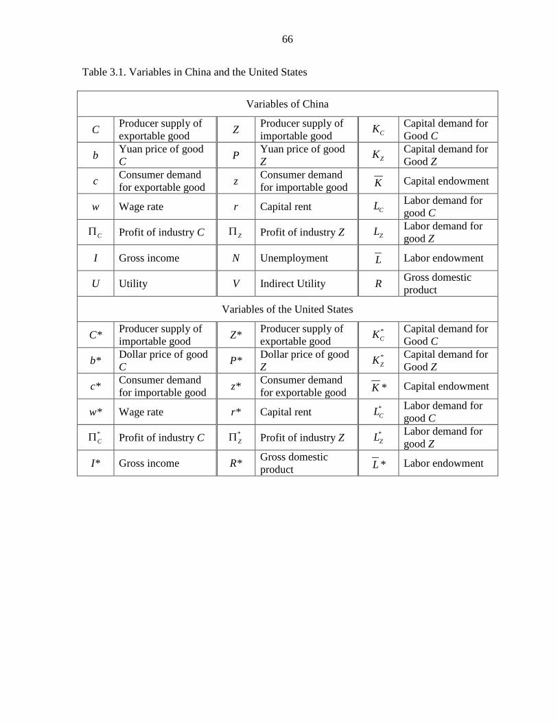
66

Table 3.1. Variables in China and the United States

Variables of China

C Producer supply of exportable good Z Producer supply of

importable good CK Capital demand for Good C

b Yuan price of good C P Yuan price of good

Z ZK Capital demand for Good Z

c Consumer demand for exportable good z Consumer demand

for importable good K Capital endowment

w Wage rate r Capital rent CL Labor demand for good C

CΠ Profit of industry C ZΠ Profit of industry Z ZL Labor demand for good Z

I Gross income N Unemployment L Labor endowment

U Utility V Indirect Utility R Gross domestic product

Variables of the United States

C* Producer supply of importable good Z* Producer supply of

exportable good *CK Capital demand for

Good C

b* Dollar price of good C P* Dollar price of good

Z *ZK Capital demand for

Good Z

c* Consumer demand for importable good z* Consumer demand

for exportable good K * Capital endowment

w* Wage rate r* Capital rent *CL Labor demand for

good C *CΠ Profit of industry C *

ZΠ Profit of industry Z *ZL Labor demand for

good Z

I* Gross income R* Gross domestic product L * Labor endowment

67

CHAPTER 4. PUBLIC CAPITAL AND OPTIMAL TARIFF

4.1 Abstract The objective of this paper is to address the relationship between the government

expenditure in public capital stock and economic growth and examine an optimal import

tariff for increase in public capital stock in a small open economy. The study provides

theoretical model of the positive impacts of public capital on production sector. It also

evaluates the effects of private capital investment on the export sector for labor and capital

formation and identifies the contribution of public capital and other economic factors to the

productivity growth rate in the firm sector. We show that the optimal tariffs are positive but

decreases to the steady state level. Since the initial public and private capital stocks are lower

than the levels of the steady state, the representative household spend more time to produce

the exportable goods to obtain higher income compare to the level of the steady state.

Increases in the public and private capital stock drops the share of labor in the export sector

and the consumer spend his/her time on the home good sector.

4.2. Introduction

In many developing counties, lack of public infrastructures such as highways,

transportation, power and water system is slowing economic growth because the

infrastructure systems are crucial input factors for domestic production. Public investment

plays an important role and a major policy issue in developing countries. A number of studies

support that public capital has a powerful impact on the productivity of private capital.

Aschauer (1989) insists the public capital is more important in determining productivity.

68

Barro (1990) also finds a positive relationship between public investment and output growth.

Recently, they found that the public capital stock and economic growth is significantly

connected especially in small income countries.

In the theoretical literature, government expenditure is introduced as an argument in

the production function as an externality in production. This approach of including public

capital in a private production function was proposed in Arrow and Kurz (1970) and all

government investment was used for productions in the private sector. To invest in public

capital, government uses two types of policies: domestic policy (income taxes or

consumption tax) or international policy (import tariff) to finance government expenditure.

Barro (1990) develops a simple model of endogenous growth in which the government uses

tax revenue and found that all government spending was productive. Abe (1990, 1992)

examined the theory of tariff reform in a small open economy. He examined that if the public

production is complementary with the private goods, then the reduce tariffs increases welfare.

However, if public production uses public inputs, then the welfare effect of lowering tariff is

not clear.

The objective of this paper is to address the relationship between the government

expenditure in public capital stock and economic growth and examine an optimal import

tariff for increase in public capital stock in a small open economy. This practice explains

rationale for government provision of public goods based on the market failure, internalizes

externalities in the private production function. Moreover, the paper is alternatively

answering "Why does the government devalue its own currency and change the terms of

trade in the short run? " The effect of change in exchange rate is the similar to that of import

tariffs which changes the relative price in domestic economy. This distortion of government

69

policy discourages current consumptions for import goods and encourage consumptions of

home goods and capital investments.

We consider a small open economy with three types of agents: household, firm and

government. The household saves in the form of capital and lends to the firm, and produces a

nontraded good or home good with only labor. The firm borrows labor and capital and

produces an export good given public capital. The government imposes an import tariff to

finance public service or public capital which is an input in the tradable output sector. The

paper begins by deriving the equilibrium in a social planning problem, characterizing its

steady-state and dynamic properties. The effects of import tariff shocks in such an economy

are analyzed. An important aspect of our analysis concerns the design of an optimal tariff

policy in an economy with gradually accumulating public capital.

We assume discrete time, infinite time-horizons and perfect foresight. The

government chooses the path of the tax rate once and for all on date 0 by taking into account

the competitive equilibrium. First, we present the competitive equilibrium and then solve the

primal problem. Our framework builds on the approach to optimal taxation. This approach

characterizes the set of allocations that can be implemented as a competitive equilibrium with

distorting taxes by two simple conditions: a resource constraint and an implementability

constraint. The implementability constraint is the household budget constraint in which the

first-order conditions are used to substitute out for tariff policies. Thus both constraints

depend only on allocations. The

study provides theoretical model of the positive impacts of public capital on production

sector. It also evaluates the effects of private capital investment on the export sector for labor

70

and capital formation and identifies the contribution of public capital and other economic

factors to the productivity growth rate in the firm sector.

Section 2 introduces the basic economic model with public capital stock and import

tariffs. Section 3 investigates the optimal tariff rates through the primal approach. Section 4

suggests the algorithm to computing the optimal import tariff sequence. Section 5 offers a

numerical analysis with log-linear Cobb-Douglas utility function to illustrate the case of

positive optimal tariffs and increasing consumer’s welfare. Section 6 provides concluding

remarks.

4.3. Basic Economic Model

We assume discrete time, infinite time-horizons and perfect foresight. The

government chooses the path of the tax rate once and for all on date 0 by taking into account

the competitive equilibrium. First, we present the competitive equilibrium and then solve the

primal problem. Our framework builds on the approach to optimal taxation. This approach

characterizes the set of allocations that can be implemented as a competitive equilibrium with

distorting taxes by two simple conditions: a resource constraint and an implementability

constraint. The implementability constraint is the household budget constraint in which the

first-order conditions are used to substitute out for tariff policies.

We now consider a two-sector small open economic model producing the non-

tradable good and the tradable good, h and x . The domestic consumers import foreign

goods, m.

The Household

The representative household's preferences are given by

71

0

1

( , ), subject t

( ) (1 ) ,(1 ) (

o

1 ) .h t t

t mt t t t t k

ht t

t

m

c l B lc k w l r

c c

k

U u

γ

τ δ

∞

+

= −+ + = + + −

=∑ (65)

where ( , )ht mtu c c is the one-period utility function and 0 < 1β < is the discount rate. htc and

mtc are consumptions in home goods and imported goods (h and m) at date t. The

representative household has a unit of time endowment. In period t, a fraction tl of the time

endowment is allocated to work in the exportable sector and the remaining fraction 1 tl− is

allocated to the domestic sector. The utility (.)u is strictly increasing in consumptions, hc

and mc , and strictly concave.

The household owns technology for producing the home good hc on date t described

as

( ) (1 ) ,h t tc l B l γ= − (66)

where the fraction 1 tl− is allocated to the home good sector and γ is a productivity parameter.

The home good hc is non-tradable and the consumption of the nontraded home good is the

same as the production of the home good.

The household earn incomes from the labor ( tl ) of the export sector and capital ( tk )

at time t. Households own capital ( tk ) and rent it to firms. The capital depreciates at a rate of

.kδ Denote that w and r are the market-determined the wage rate for labor and the rental rate

of capital from producers. The representative household budget constraint is

1(1 ) ( 1 ) ,t mt t t t t k tc k w l r kτ δ++ + = + + − (67)

72

where tτ is the rate of tariff levied by the government, 1t tq τ≡ + is the price of the

importable, and kδ is a depreciation rate of private capital stock.

The household maximizes its utility (65), subject to the technology of home good (66)

and the budget constraint (67) and the problem is written as:

1{ ,

1 0

, } 0max ( , ), su

( ) (1 ) ,(1 ) ( 1

bject to

) given .

mt t t

h

ht mt

t t

t mt t

k

t t k t

c

t

l

c l B lc k w l r k k

U u c c

γ

τ δ

+

∞

+

= −+ + = + + −

=∑ (68)

China produces two goods, using two factors: capital (K) and labor (L) inputs.

The first order conditions with respect to ,mtc tl and 1tk + are given by

: ( , ) (1 ),mt m ht mt t tc u c c λ τ= + (69)

: ( , ) ,t l ht mt t tl u c c wλ= − (70)

1 1( 1 ) .t t k trλ β δ λ+ += + − (71)

where (.) 0,lu < and (.) 0mu > are marginal utilities of labor allotted in the home good

sector and the import good.

To simplify these conditions, (69) and (70) together yield, the consumption-labor trade off

condition, the intratemporal condition,

( , ) ( , ).(1 )

tl ht mt m ht mt

t

wu c c u c cτ

− =+

(72)

Next, combining (69) and (71) yield the consumption Euler equation, the intertemporal

condition as follows:

73

11 1

1

(1 )( 1 )( , ) ( , ).(1 )t t k

m ht mt m ht mtt

ru c c u c cβ τ δτ+

+ ++

+ + −=

+ (73)

With a No-Ponzi condition 1

0 1

lim 0 ,( 1 )

TT

tT t s t k

kr δ

+

→∞= =

= Π + −

∑ the budget condition reduces to

[ ]1 0 00 1

1 (1 ) ( 1 ) .( 1 ) t mt t t kt

t s t k

c w l r kr

τ δδ

∞

+= =

+ − = + −Π + −∑ (74)

The Firm

The firm produces an exportable good at the world at price tp which is normalize,

i.e., 1tp = for all t = 0,1,⋅⋅⋅, ∞. The production function of the exportable good on date t is

1( , , ) ,t t t t t tx f G k l AG k lϕ θ θ−= = (75)

where G and k are public and private capital stocks, and ϕ and θ are productivity

parameters of the public and private capital stocks. Firm takes the public capital stock G as

given.

The production function is a constant returns to scale with private inputs, capital ( )k and

labor ( ).l Producer hires labor and rents capital from the household and pays the wage and

the capital rent to household.

Firm's profit at time t is

, , .( )t t t t t t t tf G k l w l r kπ = − − (76)

where tw and tr are the market-determined wage rate for labor and the rental rate of capital.

The firm’s optimal conditions for private capital and labor are as follows:

( ) 1 1, , ,t k t tt t tt Ar f G k l G k lϕ θ θθ − −= = (77)

74

( ) ( ) 11, ., t tt tt l t tw AG kf G k l lϕ θ θθ − −−= = (78)

Since the production function is constant returns to scale and competitive pricing ensures that

these returns are equal their marginal products, the equilibrium profits are zero.

The Government

Denote by tG the public capital stock with Gδ its depreciation rate. The government

finances its stream of purchases public capital 0{ }t tG ∞= by levying time varying tariffs on

import goods at rate tτ . Since the government has a borrowing constraint at each period, the

government budget constraint in each period is:

1 (1 )t G t t mtG G cδ τ+ − − = (79)

where Gδ is the depreciate rate for public capital stock and 0 1,Gδ< < and mtc is the

consumption of the importable good.

Comparative Equilibrium

We assume that all markets are perfectly comparative. The central planer faces an

aggregate goods market constraint and using (67), (77), (78), and (79), the resource constrain

is obtained by

1 1 ( ) (1 ) (1 ., , )mt t t G t tt t ktf G k lc G k G kδ δ+ ++ + = + − + − (80)

Given the paths of the government policy instruments 0{ }, t tt Gτ ∞= and initial

conditions for G₀ and k₀, a comparative equilibrium is household’s choices 01{ }, ,mt t t tc l k =+∞ ,

firm’s choices 0{ },t t tl k ∞= , and prices 0{ },t t tw r ∞

= , such that: (i) the household optimizes, (72) and

75

(73); (ii) the firm optimizes, (77) and (78); (iii) the government budget constraint, (79); (iv)

the goods market clears, (80).

In equilibrium, by using the firm’s optimal condition of capital in (78), the

intratemporal condition in (72) becomes

( ), ,( , ) ( , ).

(1 )l t t t

l ht mt m ht mtt

f G k lu c c u c c

τ− =

+ (81)

Moreover, by using the firm’s optimal condition of capital in (77), the intertemporal

condition in (73) becomes

( )( )

1 11

(1 ) 1( , ) ( , ).

(1,)

,kt km t mt m h

t t tt mt

t

f G k lu c c u c c

β τ δτ + +

+

+ + −=

+ (82)

Thus, we obtain new equilibrium conditions, (80), (81), and (82) in terms of , , ,tm tt Gc k and tl .

4.4. Ramsey Optimal Tariff

To solve the Ramsey planer’s problem where the government chooses allocations,

1, , ,m tt tc Gl + and 1tk + , rather than tariff rates, tτ , first, by the process of recursively using

successive household budget constraints (67) to eliminate successive 1tk + terms for t=0,⋅⋅⋅,∞,

we have

[ ] ( )( )100

01 10 0

(1 )lim 1 .

( 1 ) ( 1 ), ,t mt t tt

kt tT ts t k s t kk

c w lk kr

f G lr

kτ

δδ δ

∞+

→∞== =

+ −+ = + −

Π + − Π + −∑

76

By imposing the transversality condition (No-Ponzi Condition) for capital stocks, i.e.,

1

0 1

lim 0 ,( 1 )

TT

tT t s t k

kr δ

+

→∞= =

= Π + −

∑ we obtain the household's present budget constraint as

follows:

[ ] ( )( )0 0 0 00 1

(1 )1 .

(, ,

1 )t mt t t

ktt s t k

kf G kc w l

rl k

τδ

δ

∞

= =

+ −= + −

Π + −∑ (83)

If we use new household’s intratemporal constraint (81) and intertemporal constrain (82), we

have

01 0

0

( , ) (1 ),( , )

(1 ) ( ( , )(1 ) .(

1)

),

l ht mtt

m ht mt

t tt s

t t

m ht mt

ms k

h m

u c cu

w l

u cc

c

u

c

r cc

τ

τ δ β τ=

= −

+=

+

+ Π − +

Substitute these equations into the household's present budget constraint (83), we obtain the

implement constraint:

[ ] ( )( )0 0 0

0

0 0 0

0

1( , ) ( , ) .

, , ( , )(1 )

ktm ht

kmt mt l ht

m h mmt t

t

ku c

f G k l u c cc c u c c l

δβ

τ

∞

=

+ −− =

+∑ (84)

The Ramsey problem is as follows. The central planner chooses 1, , ,m tt tc Gl + and 1tk + ,

in order to maximize the representative household’s utility in (65) subject to the

implementability constraint (84) and the resource constraint (80).

Optimal Tariff

In the primal approach, the central planner chooses 1 1 0{ , , , }mt t tt tG klc ∞+ + = in order to

maximize the representative household’s utility in (65) subject to the implementability

77

constraint (84) and the resource constraint (80). Let µ be the Lagrange multiplier on the

impelmentability constraint (84) and define new preference function W to include the

implementability constraint as follow:

[ ]( , ) ( , ) ( , ) ( , )ht mt ht mt m ht mt mt l ht mt tW c c u c c u c c c u c c lµ= + − (85)

The Ramsey problem is

( )( )

[ ]

1 0

0 0 0 0 0

{ , , } 0

0

0

1 10

0 0

, , 1

( ) (1 ) (1 )

and given

( , )max ( , )

(1 )

, ,

.

t t t tm

k mkt

tt G t

h mht mt

c

t k t t mtt

l k

t t t

f G k l ukW

G G k k c

c cc c

k

k G

f G l

δβ

τ

β φ δ δ

µ∞

+ =

∞

+ +=

∞

−+

+ −

+ + − − + − − −∑

∑

(86)

where tφ is the Lagrange multiplier on the resource constraint at time t.

The first order conditions for this problem are for 1,t ≥

: ( , ) 0,mt ht mm ttc cW c φ =− (87)

: ( ) 0( ) , ,, ,t l tht mt l t t tc cl f G k lW φ =− (88)

[ ]1 1: ( ), , 1 0,tt t GG tt tf G lG kφ βφ δ+ +− + + − = (89)

[ ]1 1: ( ), , 1 0,tt t kk tt tf G lk kφ βφ δ+ +− + + − = (90)

1 1( ) (1 ) (1 ) 0., , G t t k t t mtt t t Gf G k l G k k cδ δ+ ++ − − + − − − = (91)

The Ramsey Allocations

Combining the optimal conditions, (87) and (88), we obtain an intratemporal

condition:

( , ) , ,( , )

( ).ht mtl t t t

ht mt

l

m

WW

c c f G k lc c

− = (92)

78

Moreover, using (87) and (90), we obtain an intertemporal condition:

[ ]1 1

( , ) ( ), , ,(

1, )

ht mtk t t t

ht mk

t

m

m

c c f G k lc

WW c

β δ+ +

= + − (93)

Equation (92) shows that the government's marginal rate of substitution between

consumption of import goods and labor in the export sector equals to the marginal product of

labor in the exportable good at date t. Similarly, equation (93) equates the government's

marginal rate of substitution between consumption today and consumption tomorrow to the

gross capital return (net of depreciation).

The optimal tariff can be determined by substituting the Ramsey allocation into the

equilibrium conditions. Combining the household’s intratemporal constraint (72), the firm’s

first order condition for labor (78) and the planer’s intratemporal constraint (92), we solve

out for the optimal tariff for 1t ≥ as follows:

* ( , ) ( , )( , )

1.( , )

ht mt ht mt

ht mt ht mt

m lt

m l

u WW u

c c c cc c c c

τ = − (94)

Now we consider a separable utility function:

1( , ) ln( ) ln ln(1 ) (1 ) ln ,ht mt ht mt t mtu c c c c B l cα α α γαγ α−= = + − + − (95)

where α and (1 )α− are the shares of expenditure on the home good and the importable good.

Then ( , )ht mtW c c can be written as

ln ln(1 ) (1 ) ln (1 )( , ) .1

tt mt

tht mt

lB l cW c cl

α γαγ α µ α αγ αγ

+ − + − + − + − − = (96)

Differentiating (96) with respect to mtc and tl , we obtain

79

1( , ) ,m ht mtmt

W c ccα−

= (97)

2

(1 )( , ) .(1 )

tl ht mt

t

lW c cl

αγ µ αγ+ −= −

− (98)

Substituting (97) and (98) into the optimal tariff, (94), for 1,t ≥ then the optimal import tariff

is

** .

1ttl

µτ =−

(99)

This implies that under the linear log utility function given by (95), we find that the optimal

tariffs are positive.

4.5. An Algorithm for Computing Optimal Import Tariff Sequence

We compute the sequence of optimal tariffs and evaluate welfare gains through the

following five steps:

First, from the Ramsey problem, we find the system of equations at the steady state

given by four first order conditions and the planner's resource constraint as follows:

(1 ) 0,mss

sscα φ−−

= (100)

( ) 12

(1 ) 1 0,(1 )

ssss ss ss ss

ss

l AG k ll

ϕ θ θαγ µ αγ φ θ − −+ −− − =

− (101)

1 11 1 0,ss ss ss GAG k lϕ θ θβ ϕ δ− −− + + = − (102)

1 11 1 0,ss ss ss kAG k lϕ θ θβ θ δ− −− + + = − (103)

80

1 0.ss ss ss G ss k ss mssAG k l G k cϕ θ θ δ δ− − − − = (104)

In this system, there are six variables, , , , , ,ss ss ss ss mssG k l cφ and µ . However we have only

five equations. We assume that in the steady state, 1/ 3ssl = and we solve the systems for the

five unknown variables. The optimal values at the steady state as follows:

11 1 1

1 ,(1 (1 )) (1 (1 ))

ssss

k G

AlGθ θ θ θ ϕ

θ θ

βϕ θβ δ β δ

− − − −

−

= − − − −

(105)

11 1 1

1 ,(1 (1 )) (1 (1 ))

ssss

k G

Alkϕ ϕ θ θ ϕ

ϕ ϕ

βϕ θβ δ β δ

− − − −

−

= − − − −

(106)

1 ,mss ss ss ss G ss k ssc AG k l G kϕ θ θ δ δ−= − − (107)

(1 ) ,ssmsscαφ −

= (108)

( ) 1 21 (1 )1.ss ss ss ss ss

ss

AG k l ll

ϕ θ θφ θµ

αγ

− −− −= + − (109)

From the steady state, we obtain the value of the Lagrange multiplier µ which depends on

.ssl

Second, having computed the steady –state allocations, the Lagrange multiplier µ , we look

at the first order conditions and the resource constraint for 1,t ≥ which are given by

(1 ) 0,mt

tcα φ−−

= (110)

( ) 12

(1 ) 1 0,(1 )

tt t t t

t

l AG k ll

ϕ θ θαγ µ αγ φ θ − −+ −− − =

− (111)

1 1 11 1 0,t t t t t GAG k lϕ θ θφ βφ ϕ δ− − −+ − + + − = (112)

81

1 11 1 1 1 1 0,t t t t t kAG k lϕ θ θφ φ β θ δ− −+ + + +− − + + = (113)

11 1(1 ) (1 ) 0.t t t t G t t k ss mtAG k l G G k k cϕ θ θ δ δ−+ +− + − − + − − = (114)

Since Lagrange multiplier μ is obtain from the steady state, we have seven unknown

variables, 1 1 1, , , , , ,t t t t mt tG k l l c φ+ + + and 1tφ + , and five optimal equations.

Using the optimal equations (110)-(114), we obtain two dynamic equations 1tk + and 1tG + as

follows:

1 1( ) (1 ) (1 ) ,k G t t

t t G t k ss mtt t

G kG k G k cG k

δ δ δ δθ ϕ+ +

−+ = + − + − −

− (115)

[ ]

11 1

11

11

1 1 11 1 1

21 1 11 1 1

1 1 1

1 1 11 1 1

1 1 1

(1 ) ( ) ( ) ( )

( ) ( ) ( ) (1 )( )

(1 ) ( ) ( )

t t k G t t t t t

t t k G t t k G t G t t

t t k G t t

A G k G k G G k

A G k G k k G k

A G k G k

ϕ θ ϕθ θ

ϕθ

ϕθ

θ θ θ

θ θ θ

θ θ θ

µ θ ϕ δ δ θ ϕ

θ ϕ δ δ β ϕ δ δ δ θ ϕ

µ θ ϕ δ δ

− −− −

−−

−−

− − −

− − −+ + +

− − −+ + +

+ − − − −

− − − − + − −

+ − − −=

1

11

1 1

21 1 11 1 1

1 1 1 1

.

( ) ( )

t

t t k G t t

G

A G k G k

θ ϕθ

ϕθθ θ θθ ϕ δ δ

−−

−−

+ +

− − −+ + + +

− − −

(116)

Third, since the steady-state levels of public and private capitals, ssG and ssk , and

labor in the exportable sector, ssl depends on the initial values of public and private capital

stocks 0G and 0k , we guess the initial values of public and private capital stocks 0G and 0k .

After the iterations converge, the public and private capital stocks are matched with the

steady-state values obtained in the first step. If they don't, the initial guess for 0G and 0k is

corrected. This is repeated, until the iterations converge to the steady-state allocations.

82

Fourth, we use the sequence of allocations 1{ , }Tt t tG k = , to compute the entire sequence

1{ }Tt tl = by using the optimal condition

11

1 11 1

( ) .( )

k G t tt

t t

G klA G k

ϕθ

θ θ

δ δ

θ ϕ

−−

− −

−=

− (117)

Given initial public and private capital stocks 0G and 0k , if the value for ssl obtained in step

4 matches with the one given, we stop. Otherwise, the guess for ssl is updated, and steps 1-4

is repeated, until convergence is achieved.

Finally, after steps 1-4 converge, the optimal sequence of import tariffs 1{ }Tt tτ = is

obtained from

.1t

tlµτ =−

(118)

4.6. Numerical Analysis

We use a separable utility function ( , ) ln ln(1 ) (1 ) ln .ht mt t mtc c B lu cα γαγ α= + − + −

We choose parameters α = 0.4 and 3,γ = and nomalize B=1. We use the Cobb-Douglas

production function 1 1 .t t t tx AG k lϕ θ θ− −= We choose the shares of public and private capitals at

0.5ϕ = and 0.3θ = , and A=2. The annual time preference rate is 0.9,β = and the

depreciation rates of public and private capital stocks are 0.1Gδ = and 0.3kδ = . The

parameters are summarized in Table 4.1.

To solve the levels of the steady state, we assume that the level of labor in the

exportable sector is 1/ 3.ssl = Using the solutions for the steady-state, (105) - (109), we

83

obtain the steady state levels of the variables, , , , ,ss ss ss mssG k cφ and µ , where µ is the

Lagrange multiplier on the implement constraint as following Table 4.2.

From the steady state solutions, we find that the optimal tariff is 0.7041ssτ = which is

positive. We assume that the initial values of public and private capital stocks are lower than

the levels of the steady states and set and the initial values of public and private capital stock

as G₀=0.95885* ssG =1.1583 and k₀=0.97* ssk =0,6017. Using the value of the Lagrange

multiplier on the implement constraint 0.4694,µ = and the initial values, we find the

sequence of allocations of public and private capital stocks and a share of labor in the export

sector 1{ , , }Tt t t tG k l = , converge to the steady state levels and obtain the optimal sequence of

import tariffs 1{ }Tt tτ = .

Trends in the Public and Private Capital Stock

In assessing the public and private capital stocks and its relationship to output, it is

important to take into account both the volume of capital stocks (the physical amount of

capital goods) and the ratios of capital stocks to gross domestic product (GDP) each period.

Figure 4.1. and Figure 4.2. below describe that the ratios of public and private capital stocks

to GDP.

The initial ratios of public and private capital to GDP are 1.408 and 0.731 and reach to the

highest levels 1.457 and 0.73818. However, after reaches to the highest level, the ratios

slightly drop and move to the steady state levels.

The Figure 4.3. illustrates the pattern of the share of labor in the export sector. Labor income

from the export sector is the main source for household’s income. Using the income, the

household consumes import goods and increases his/her utility. In this model, we assume that

the initial levels of public and private capital stock are lower than those of the levels of

84

steady state. The lower levels of capital stocks cause lower wage and capital rent from the

private capital stock.

In order to increase household income, the consumer initially works more than the

level of the steady state. From the government investments in the public capital financed

through the import tariffs, the household increases private capital stock and reduces the share

of labor in the export sector shown in Figure 4.3. This implies that the consumers enjoy more

home goods (non-traded goods) such as gardening, home cooked meal or leisure. As the

public and private capital stock reach to the levels of the steady state, the share of labor in the

export sector also arrives the level of the steady state.

The countries endowed lower levels of public and private capital stocks initially

levies higher tariff rates for import goods. As the both capital stocks have accumulated, the

government reduces the import tariffs. Figure 4.4. provides the optimal tariff rates which are

positive even in the level of steady state. The public capital is an important input to produce

exportable goods and the higher level of a public capital stock increases the marginal product

of labor and capital that are the same as the wage and capital rent. In other words, the

increase in a public capital stock increases household’s income. Thus, the income effect of

the public capital stock is larger than the substitute effect of between shares of labor in the

exportable sector and home good sector. The consumer reduces the share in the export sector.

Finally, Figure 4.5. depicts the trends of consumer’s welfare. Increases both home

goods and import goods consumptions improve the consumers’ welfare. The level of the

welfare gradually increases and reached the level of the steady state when the allocations of

the public and private capital stocks and the share of labor in export sector stay in the levels

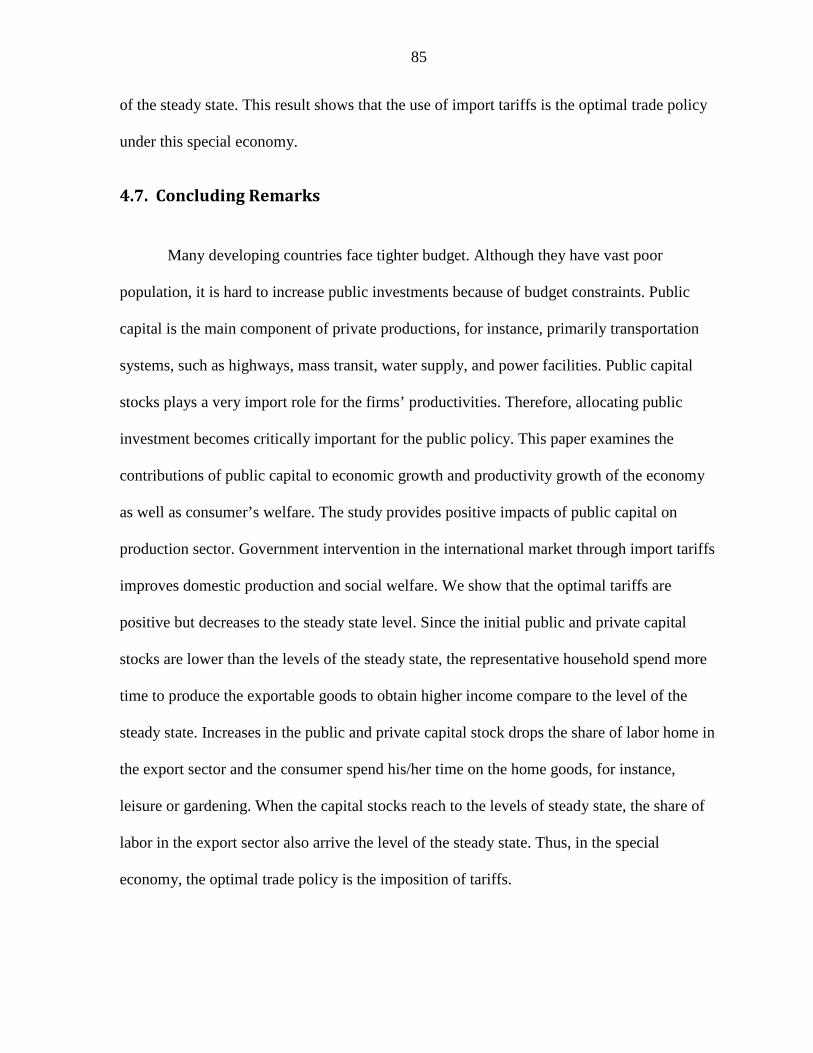
85

of the steady state. This result shows that the use of import tariffs is the optimal trade policy

under this special economy.

4.7. Concluding Remarks

Many developing countries face tighter budget. Although they have vast poor

population, it is hard to increase public investments because of budget constraints. Public

capital is the main component of private productions, for instance, primarily transportation

systems, such as highways, mass transit, water supply, and power facilities. Public capital

stocks plays a very import role for the firms’ productivities. Therefore, allocating public

investment becomes critically important for the public policy. This paper examines the

contributions of public capital to economic growth and productivity growth of the economy

as well as consumer’s welfare. The study provides positive impacts of public capital on

production sector. Government intervention in the international market through import tariffs

improves domestic production and social welfare. We show that the optimal tariffs are

positive but decreases to the steady state level. Since the initial public and private capital

stocks are lower than the levels of the steady state, the representative household spend more

time to produce the exportable goods to obtain higher income compare to the level of the

steady state. Increases in the public and private capital stock drops the share of labor home in

the export sector and the consumer spend his/her time on the home goods, for instance,

leisure or gardening. When the capital stocks reach to the levels of steady state, the share of

labor in the export sector also arrive the level of the steady state. Thus, in the special

economy, the optimal trade policy is the imposition of tariffs.

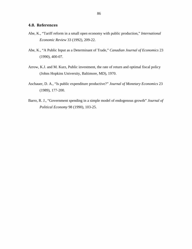
86

4.8. References

Abe, K., “Tariff reform in a small open economy with public production,” International

Economic Review 33 (1992), 209-22.

Abe, K., “A Public Input as a Determinant of Trade,” Canadian Journal of Economics 23

(1990), 400-07.

Arrow, K.J. and M. Kurz, Public investment, the rate of return and optimal fiscal policy

(Johns Hopkins University, Baltimore, MD), 1970.

Aschauer, D. A., “Is public expenditure productive?” Journal of Monetary Economics 23

(1989), 177-200.

Barro, R. J., “Government spending in a simple model of endogenous growth” Journal of

Political Economy 98 (1990), 103-25.

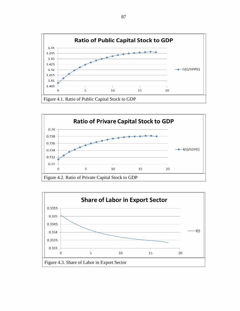
87

Figure 4.1. Ratio of Public Capital Stock to GDP

Figure 4.2. Ratio of Private Capital Stock to GDP

Figure 4.3. Share of Labor in Export Sector

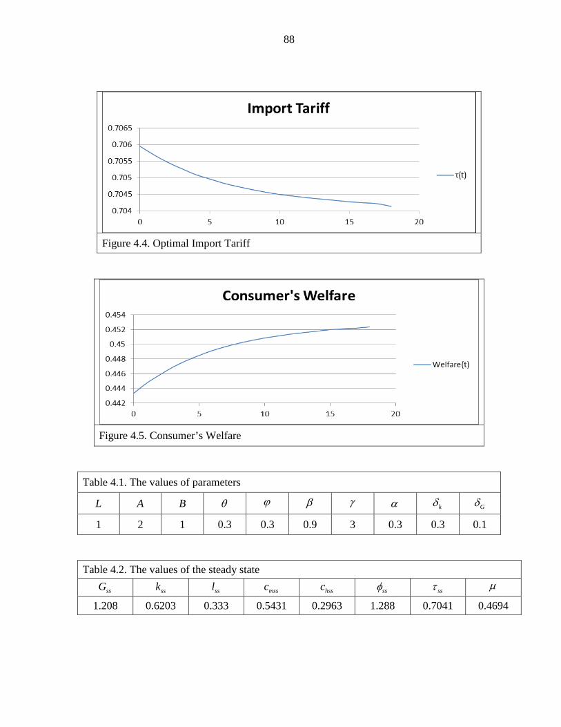
88

Figure 4.4. Optimal Import Tariff

Figure 4.5. Consumer’s Welfare

Table 4.1. The values of parameters

L A B θ ϕ β γ α kδ Gδ

1 2 1 0.3 0.3 0.9 3 0.3 0.3 0.1

Table 4.2. The values of the steady state

ssG ssk ssl mssc hssc ssφ ssτ µ

1.208 0.6203 0.333 0.5431 0.2963 1.288 0.7041 0.4694

89

CHAPTER 5. CONCLUDING REMARKS

China has been accused of intentionally depressing the value of its currency, the

renminbi, to gain unfair advantages in the global market. If producers and consumers in both

countries act as price takers, the equilibrium prices of the traded goods are determined by the

supplies and demands in the world market, and the benchmark yuan value of the dollar is

determined in a competitive market. An important policy question is whether China will

benefit from devaluing the yuan from the benchmark equilibrium rate. An optimal exchange

rate may depend on the exchange rate pass-through to the yuan price of China’s exports or

the dollar price of U.S. imports. As the yuan peg is raised, the exchange rate pass-through

may not be perfect. If the yuan price of China’s export rises more than proportionately, then

China’s optimal policy is a yuan devaluation. China’s elasticity of the export price index with

respect to exchange rate has been less than unity since 2003. This implies that China’s yuan

devaluation policy has been consistent with the prediction of the main proposition.

While tariffs and non-tariff barriers are bound by various agreements in the WTO,

there are no such agreements among countries on the bilateral exchange rates. The IMF

monitors only the exchange rates of developing countries that are beset by large balance of

payments deficits. The WTO regulates only tariff and various non-tariff barriers, but has

made little effort to regulate the bilateral exchange rates because exchange rate practices are

within the purview of the IMF. The finding that tariffs and the undervalued yuan have the

same effects on domestic prices and import volumes suggests that currency pegging can be

viewed as a trade policy. Either the WTO or IMF could begin to consider regulation of

90

currency practices of developing countries in the face of large trade imbalances between

major trading countries.

i Jin and Choi (2013) noted that while in the short run some profits might be generated by slightly deviating from the equilibrium exchange rates, in the long run excessive hoarding of reserve assets can only result in huge losses to PBC’s balance of payment account. ii If the equilibrium exchange rate is 6 (6 yuan = $1), then new renminbi can be issued so that 6 old yuan = 1 new yuan. With this currency conversion, the equilibrium dollar price of the new renminbi is 1. In the empirical work, we relax this assumption to derive the equilibrium exchange rates in each period.

iii In empirical analyses the value of oε cannot be fixed arbitrarily, but must be derived from the balanced trade condition.

iv The Chinese currency devaluation may not be the only source of U.S. trade deficits. For instance, Beladi and Oladi (2014) suggest that outsourcing may widen U.S. trade deficits. Also, Yue and Zhang (2013) emphasize that the U.S. trade deficit would not be reduced very much by a change in the Chinese exchange rate.

v Of course, the first-best policy is to remove wage and rent rigidity in the factor markets. Given this rigidity, Chinese government may be using yuan devaluation as a second-best policy.

vi In the same vein, Bruno (1976) considered a two-sector model, but defined the exchange rate as the ratio of the price of the tradable good to that of the nontradable good.

vii See Holtemöller and Mallick (2013) for a model of currency misalignment. They show that the higher the flexibility of the currency regime, the lower is the misalignment.

viii Devereux (2000) analyzed the impact of devaluation on the trade balance when exchange rate pass-through is imperfect.

ix For instance, if China is abundant in labor and production of C is labor-intensive, China is expected to export good C and import good Z.

x For instance, 1 121 1( 1) 0,LL C C CF A L Kα βα α −= − < 1 1 2

1 1( 1) 0,KK C C CF A L Kα ββ β −= − < 1 11 1

1 1 0,LK C C CF A L Kα βα β − −= > and ( ) ( )1 122 1 1

1 1 1 1(1 ) 0.LL KK LK C C CF F F A L Kα βα β α β − −− = − − >

xi Money as a financial instrument does not enter the utility function directly, but indirectly through a change in income, which ultimately affects consumption. See Al-Abri (2014) for a model in which utility depends on money balances.

91

xii If the benchmark equilibrium value of $1 is 6 RMB, new RMB notes can be issued at the rate of 6 RMB for 1 new RMB.

xiii1 12 2 1 12 2

2 2 1 1

1/(1 )1/(1 )

1 12 2 (1 ) CZ b AAw r w r

α βα β α βα β

α β α β

α βδα βγ γ− −− −

= −

xiv1 12 2 1 12 2

2 2 1 1

1/(1 )1/(1 )

1 12 2 (1 ) CZ b AAw r w r

α βα β α βα β

α β α β

α βδα βγ γ− −− −

= −

xv It can be shown that

1 12 2 1 1

1 1

1 1 2 21 1 2 2

1 1 2 2

1 1

1 1 2

0 3 2 41

1/(1 )12 2 1 1 2 2

2 2 1 1 2 2

1/(1 ) 1/(1 )

1 1 2 2

11 1

( ) ( ) ( *) ( )*1(1 ) (1 )( )

* *C Z

A A A A

w rw r

A Aw r w r

α βα β α β

α β

α β α βα β α β

α β α β

α βα β α

α β δ α β α β δ δα β α β α β

α β α β

δ δ

− −− −

− − − −

+− − −

−

+ + − −= − − − − − +

×

−1 1 2 21 1 2 2

2

1 1 2 2

1 1 2 21 11 1 2 2

1 1 2 2

1/(1 ) 1/(1 )

1 11 1 2 2 2 2

1 1 2 2

11/(1 ) 1/(1 )1

1 11 1 2 2

1 1

( ) ( )(1 )(1 )

( ) .1 * *

C Z

C Z

A Aw r w r

A Aw r w r

α β α βα β α ββ

α β α β

α β α βα βα β α β

α β α β

α βα β α β α βα β α β

α βδ α β α βα β

− − − −

−

− − − −− −

+ − + − − − −

+− − −

xvi Jiang and Kim (2013) show that exchange rate pass-through to the producer price index and the retail price index are both incomplete. Without concavity of ( ),b δ multiple optimal exchange rates may exist, including the exchange rate that yields some unemployment.

xvii Under assumption / 0,r δ∂ ∂ > the effects of the exchange rate on output C and Z are

( )

1 11 1 1 1 1 1

1 1

1 11 1 1 1 1 1

1 1

2 2 2 2

2 2

11 1 1 1 1

1 1

11 1

1 1 11 1

2 2

2 2

( )( , ) 1 11

1 1( ) ,1

Z( , ) 11

C

Cb r

Z

b AC b P b rw r b r

b Aw r

P Ab Pw r

α βα β α β α β

α β

α βα β α β α β

δ δα β

α β α β

α β

α β α β δ β δδ α β δ δ δ

α β α β ε β εα β δ

α βδ α β

++ − −

++ − −

+

+∂ ∂ ∂ = − ∂ − − ∂ ∂

= − + − − −

∂= ∂ − −

( )2 2

2 21

2 2 21( ) 0.P r

α βα β

δ δα β ε β εδ

+− −

+ − >