Three-Pot Household Water Treatment System: Testing the

Developing

knowledge and capacity

in water and sanitation

Water, Engineering and Development Centre

Loughborough University, UK

Three-Pot Household Water Treatment System:

Testing the Effectiveness

by

Katerina Chegkazi

A research project submitted in partial fulfillment of the requirements for

the award of the degree of Master of Science of Loughborough University

August 2012

Supervisor: Mr. Brian Skinner - BSc CNAA, MSc Loughborough, CEng, MICE

i

Three-Pot Household Water Treatment System:

Testing the Effectiveness

by

Katerina Chegkazi

August 2012

Supervisor: Mr. Brian Skinner

BSc CNAA, MSc Loughborough, CEng, MICE

ii

Acknowledgments

A long and tiring, but fruitful academic year is coming to its end with the present project.

People I’d like to thank for this year and this project in specific...

My family and friends back home, always supporting my decisions by any means.

The friends I’ve made in this country, here to listen and comfort one another.

Brian Skinner, as my supervisor on this project, for his valuable guidance, efficient feedback

and yet discrete presence, allowing space for new ideas. But also, as my personal tutor

throughout the year, always being the voice of logic, helping me see things more realistically.

Brian Reed, for all his thought triggering ideas, inside and outside the classroom.

Sue Coates, for being an inspiration from the first day.

The WEDC team, for being true professionals.

Jayshree Bhuptani and Geoffrey Russell from the laboratory, for providing their valuable

knowledge and help, without complaining.

The year itself, for being one more great chance to get to know ourselves a bit better.

God and nature, for still being with us, giving their wisdom to those who want to listen.

Last, I would like to dedicate all my efforts to those people, those memories and those

emotions that will always remain in our hearts, no matter where we are and what we

experience. These make us who we are. Thank you μ for being in my heart. I will always keep

you there…

v

Table of contents

Acknowledgments ........................................................................................................................ ii

Certificate of Authorship .............................................................................................................. iii

Individual Research Project Access Form .................................................................................. iv

Table of contents .......................................................................................................................... v

List of Figures ............................................................................................................................ viii

List of Graphs .............................................................................................................................. ix

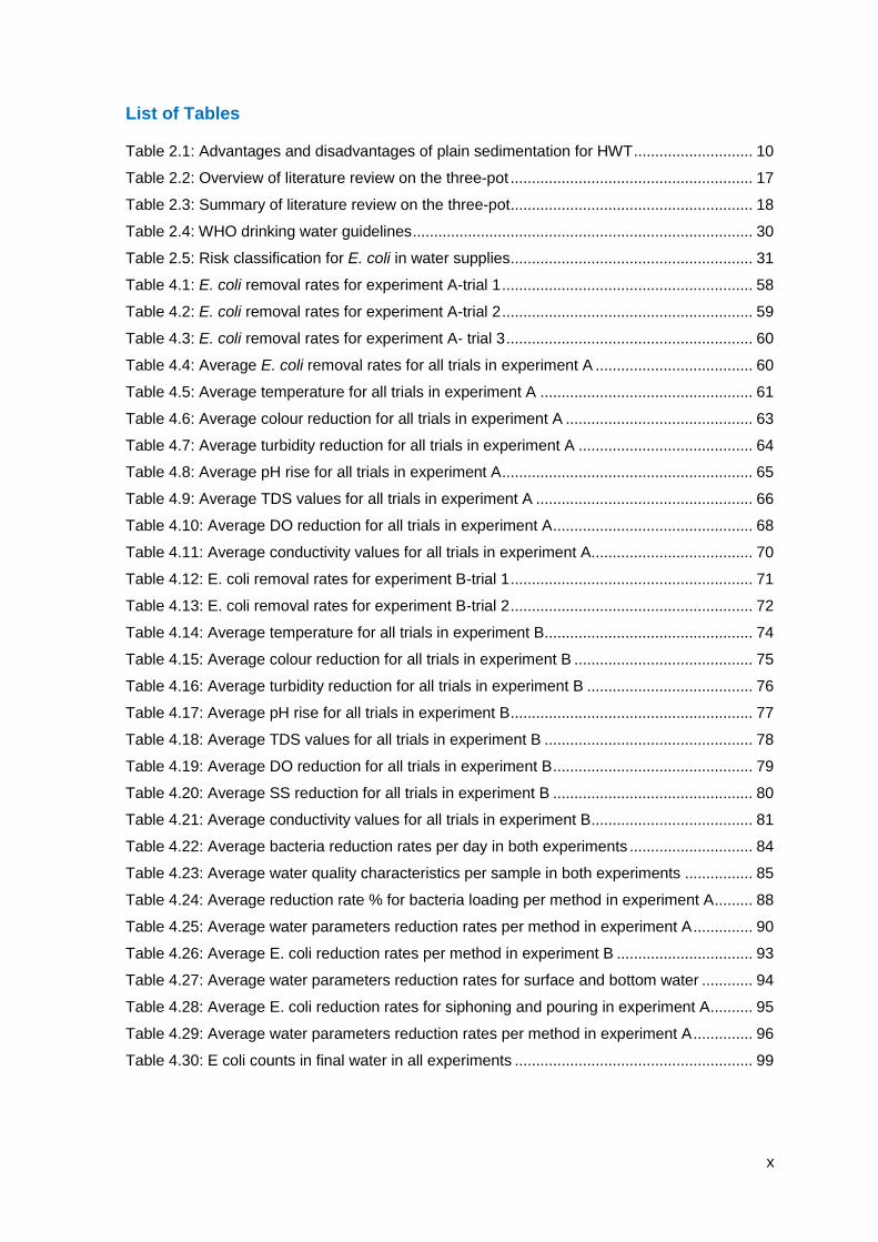
List of Tables ................................................................................................................................ x

Acronyms, Abbreviations and Units ............................................................................................ xi

1.0 Introduction ............................................................................................................................ 1

1.1 Background ........................................................................................................................ 1

1.2 Research Contribution, Aim and Objectives ..................................................................... 2

1.2.1 Research Contribution ............................................................................... 2

1.2.2 Research Aim ............................................................................................ 3

1.2.3 Research Objectives ................................................................................. 3

1.3 Project’s Structure ............................................................................................................. 3

2.0 Literature Review................................................................................................................... 4

2.1 Household Water Treatment and Safe Storage ................................................................ 4

2.1.1 Definition and Background ........................................................................ 4

2.1.2 Significance, Applications and Limitations ................................................ 5

2.1.3 Sedimentation in Household Water Treatment Systems .......................... 7

2.2 The Three-Pot Water Treatment System ........................................................................ 11

2.2.1 Definition and Background ...................................................................... 11

2.2.2 Overview of Literature on Three-Pot ....................................................... 13

2.2.3 Design Characteristics ............................................................................ 18

2.2.4 Purification Mechanisms ......................................................................... 19

2.3 Gaps in Knowledge.......................................................................................................... 24

2.3.1 Absence of laboratory experiments......................................................... 24

2.3.2 Gaps in Knowledge ................................................................................. 25

2.4 Related Issues ................................................................................................................. 27

2.4.1 Water Quantity........................................................................................ 27

2.4.2 Water Quality .......................................................................................... 28

2.4.3 Water quantity versus water quality ........................................................ 32

2.4.4 Issues related to the design characteristics ............................................ 33

3.0 Methodology ........................................................................................................................ 37

3.1 Planning Procedure ......................................................................................................... 37

3.1.1 Overview .................................................................................................. 37

3.1.2 Water source ........................................................................................... 38

vi

3.1.3 Water collection and transportation......................................................... 40

3.1.4 Water sampling........................................................................................ 40

3.1.5 Testing parameters and equipment ........................................................ 41

3.2 Testing Procedure ........................................................................................................... 48

3.2.1 Experiment A ........................................................................................... 49

3.2.2. Experiment B .......................................................................................... 52

3.2.3 Unexpected conditions ............................................................................ 54

4.0 Results and Analysis ........................................................................................................... 56

4.1 Lab Results ...................................................................................................................... 56

4.1.1 Experiment A ........................................................................................... 56

4.1.2 Experiment B ........................................................................................... 70

4.1.3 Acceptability issues ................................................................................. 81

4.2 Discussion and Analysis .................................................................................................. 83

4.2.1 What is the bacteria removal effectiveness of the three-pot system? .... 84

4.2.2 How many days should the retention time be? ....................................... 87

4.2.3 Is siphoning more effective than pouring? .............................................. 88

4.2.4 Is the surface water of better quality than the water at the bottom? ....... 92

4.2.5 How many pots should be used? ............................................................ 94

4.3 Testing the effectiveness: Discussion ............................................................................. 98

4.4 Limitations ...................................................................................................................... 102

4.4.1 Limitations of the three-pot system ....................................................... 102

4.4.2 Limitations of the project ....................................................................... 103

4.5 Review ........................................................................................................................... 105

5.0 Recommendations ............................................................................................................ 106

5. 1 Recommendations on the three-pot system ................................................................ 106

5. 2 Recommendations for future projects .......................................................................... 107

6.0 Conclusions ....................................................................................................................... 110

7.0 References ........................................................................................................................ 112

8.0 Appendices ........................................................................................................................ 122

8.1 Experiment A raw data excel sheets ............................................................................. 122

8.1.1 Trial 1 ..................................................................................................... 122

8.1.2 Trial 2 ..................................................................................................... 123

8.1.3 Trial 3 ..................................................................................................... 126

8.2 Experiment B raw data excel sheets ............................................................................. 129

8.2.1 Trial 1 ..................................................................................................... 129

8.2.2 Trial 2 ..................................................................................................... 130

8.3 Experiment A and B reduction rates tables ................................................................... 133

8.3.1 Experiment A – Trial 1 ........................................................................... 133

vii



8.3.4 Experiment B – Trial 1 ........................................................................... 134

8.3.5 Experiment B – Trial 2 ........................................................................... 135

8.4 Trial sampling prior to experiments ............................................................................... 136

viii

List of Figures

Figure 1.1: Three-pot System in the Development Pyramid ....................................................... 2

Figure 2.1: Prolonged storage ................................................................................................... 11

Figure 2.2: The three-pot treatment system .............................................................................. 12

Figure 2.3: The three-pot method ............................................................................................ 13

Figure 2.4: Design characteristics ............................................................................................. 18

Figure 2.5: Separation techniques for different particle sizes ................................................... 20

Figure 2.6: Micro-organism growth curve.................................................................................. 23

Figure 2.7: Gap in knowledge ................................................................................................... 25

Figure 2.8: Some water-related pathogens ............................................................................... 29

Figure 3.1: Map of WEDC area, showing the water source location ........................................ 38

Figure 3.2: Point of abstraction in Holywell brook ..................................................................... 39

Figure 3.3: Water collection and transportation ........................................................................ 40

Figure 3.4: Labeled Petri Dishes in series and in detail ............................................................ 44

Figure 3.5: Nalgen filter holder with receiver ............................................................................ 44

Figure 3.6: Petri dish with blue distinct colonies after MLSB medium ...................................... 45

Figure 3.7: Digital High Temperature 8’’ lab thermometer ........................................................ 45

Figure 3.8: Siemens Photometer P15 lab colour meter ............................................................ 46

Figure 3.9: Hach 2100N lab turbidity meter .............................................................................. 46

Figure 3.10: Hanna Instrument HI9812 ..................................................................................... 46

Figure 3.11: Suspended solids Glass microfiber paper filters in use ........................................ 47

Figure 3.12: YSI Model 58 dissolved oxygen lab meter .......................................................... 48

Figure 3.13: Experimental setup A ............................................................................................ 50

Figure 3.14: Labels, distinctive lines and arrows separating the three-pot systems ................ 50

Figure 3.15: Siphon used for the experiments .......................................................................... 52

Figure 3.16: Experimental setup B ............................................................................................ 53

Figure 4.1: E. coli colonies in water .......................................................................................... 56

Figure 4.2: Small leaves (a) and a dead bug (b) floating on the surface .................................. 82

Figure 4.3: Algal ring near the surface ...................................................................................... 83

Figure 4.4: Syringe clearing out the centre of the pot ............................................................... 92

Figure 4.5: Colour with a naked eye in undisturbed (a) and decanted (b) water...................... 97

ix

List of Graphs

Graph 4.1: E. coli counts reduction over time in experiment A-trial 1 ....................................... 58



Graph 4.4: Temperature over time in experiment A-trial 1 ....................................................... 61

Graph 4.5: Colour reduction over time in experiment A-trial 1 ................................................. 62

Graph 4.6: Turbidity reduction over time in experiment A-trial 1 .............................................. 63

Graph 4.7: pH over time in experiment A-trial 1 ........................................................................ 64

Graph 4.8: Total Dissolved Solids over time in experiment A-trial 1 ........................................ 66

Graph 4.9: Dissolved oxygen over time in experiment A-trial 1 ................................................ 67

Graph 4.10: Dissolved oxygen before and after decanting in experiment A-trial 1 .................. 68

Graph 4.11: Suspended Solids over time in experiment A-trial 1 ............................................. 69

Graph 4.12: Conductivity over time in experiment A-trial 1 ...................................................... 69

Graph 4.13: E. coli counts reduction over time in experiment B-trial 1..................................... 71

Graph 4.14: E. coli counts reduction over time in experiment B-trial 2..................................... 72

Graph 4.15: E. coli reduction rates for transferred water in both trials in experiment B ........... 73

Graph 4.16: Temperature over time in experiment B-trial 1 ..................................................... 74

Graph 4.17: Colour reduction over time in experiment B-trial 1 ............................................... 75

Graph 4.18: Turbidity reduction over time in experiment B-trial 1 ............................................ 76

Graph 4.19: pH over time in experiment B-trial 1 ...................................................................... 77

Graph 4.20: Total Dissolved Solids over time in experiment B-trial 1 ...................................... 78

Graph 4.21: Dissolved oxygen over time in experiment B-trial 1 .............................................. 78

Graph 4.22: Suspended Solids over time in experiment B-trial 1 ............................................. 79

Graph 4.23: Conductivity over time in experiment B-trial 1 ...................................................... 81

Graph 4.24: Average reduction rates per day in both experiments .......................................... 84

Graph 4.25: Difference in the E. coli reduction rates between siphoning and pouring per day

and per sample in experiment A................................................................................................ 89

Graph 4.26: Difference in the E. coli reduction rates between bottom and surface water per

day in experiment B ................................................................................................................... 93

Graph 4.27: Difference in the E. coli reduction rates between decanted and stable water per

day and per decanting method in experiment A ....................................................................... 95

x

List of Tables

Table 2.1: Advantages and disadvantages of plain sedimentation for HWT ............................ 10

Table 2.2: Overview of literature review on the three-pot ......................................................... 17

Table 2.3: Summary of literature review on the three-pot ......................................................... 18

Table 2.4: WHO drinking water guidelines ................................................................................ 30

Table 2.5: Risk classification for E. coli in water supplies ......................................................... 31

Table 4.1: E. coli removal rates for experiment A-trial 1 ........................................................... 58

Table 4.2: E. coli removal rates for experiment A-trial 2 ........................................................... 59

Table 4.3: E. coli removal rates for experiment A- trial 3 .......................................................... 60

Table 4.4: Average E. coli removal rates for all trials in experiment A ..................................... 60

Table 4.5: Average temperature for all trials in experiment A .................................................. 61

Table 4.6: Average colour reduction for all trials in experiment A ............................................ 63

Table 4.7: Average turbidity reduction for all trials in experiment A ......................................... 64

Table 4.8: Average pH rise for all trials in experiment A ........................................................... 65

Table 4.9: Average TDS values for all trials in experiment A ................................................... 66

Table 4.10: Average DO reduction for all trials in experiment A ............................................... 68

Table 4.11: Average conductivity values for all trials in experiment A ...................................... 70

Table 4.12: E. coli removal rates for experiment B-trial 1 ......................................................... 71

Table 4.13: E. coli removal rates for experiment B-trial 2 ......................................................... 72

Table 4.14: Average temperature for all trials in experiment B................................................. 74

Table 4.15: Average colour reduction for all trials in experiment B .......................................... 75

Table 4.16: Average turbidity reduction for all trials in experiment B ....................................... 76

Table 4.17: Average pH rise for all trials in experiment B ......................................................... 77

Table 4.18: Average TDS values for all trials in experiment B ................................................. 78

Table 4.19: Average DO reduction for all trials in experiment B ............................................... 79

Table 4.20: Average SS reduction for all trials in experiment B ............................................... 80

Table 4.21: Average conductivity values for all trials in experiment B ...................................... 81

Table 4.22: Average bacteria reduction rates per day in both experiments ............................. 84

Table 4.23: Average water quality characteristics per sample in both experiments ................ 85

Table 4.24: Average reduction rate % for bacteria loading per method in experiment A ......... 88

Table 4.25: Average water parameters reduction rates per method in experiment A .............. 90

Table 4.26: Average E. coli reduction rates per method in experiment B ................................ 93

Table 4.27: Average water parameters reduction rates for surface and bottom water ............ 94

Table 4.28: Average E. coli reduction rates for siphoning and pouring in experiment A .......... 95

Table 4.29: Average water parameters reduction rates per method in experiment A .............. 96

Table 4.30: E coli counts in final water in all experiments ........................................................ 99

xi

Acronyms, Abbreviations and Units

oC………………………………………………………………………………………...Celsius degree

cfu……………………………………………………………………………….....colony forming units

cm……………………………………………………………………………………………...centimeter

DO…………………………………………………………………………………….Dissolved Oxygen

E. coli………………………………………………………………………………Escherichia coliform

EHEC…………………………………………………………..Enterohaemorrhagic Escherichia coli

ETEC…………………………………………………………………Enterotoxigenic Escherichia coli

gr……………………………………………………………………………………………...…….grams

HWT………………………………………………………………………Household Water Treatment

HWTS………………………………………………Household Water Treatment and Safe Storage

ID50…………………………………………………………..…………………median Infectious Dose

l…………………………………………………………..…………………………………………….litre

lcd…………………………………………………………..…………………..litres per capita per day

MDG…………………………………………………………………..Millennium Development Goals

mg…………………………………………………………..…………………………………...milligram

ml…………………………………………………………..…………………………………….millilitres

NTU……………………………………………………………………..Nephelometric Turbidity Units

p…………………………………………………………..………………………………………….page

POU…………………………………………………………..……………………………..Point of Use

ppm…………………………………………………………..………………………….parts per million

RR…………………………………………………………..…………………………...Reduction Rate

SODIS………………………………………………………………………………...Solar Disinfection

SS…………………………………………………………………………………….Suspended Solids

TCU…………………………………………………………………………………...True Colour Units

TDS………………………………………………………………………………Total Dissolved Solids

UN………………………………………………………………………………………...United Nations

UNICEF……………………………………………………………….United Nations Children's Fund

UV……………………………………………………………………………………………..Ultra Violet

WEDC………………………………………………..Water, Engineering and Development Centre

WHO………………………………………………………………………..World Health Organization

μS………………………………………………………………………………………...micro-Siemens

1

1.0 Introduction

1.1 Background

Water is one of the basic human needs, crucial for survival. Although two-thirds of the earth’s

surface is covered by water, only 2% of it is fresh water (Reed, 2012, p. 1.2), potentially

suitable for human needs. This small amount is often contaminated and in addition the world’s

overpopulation, industrialization and climate change exacerbate the global water shortages

(Jones, 1997, p.2).

It is commonly reported that 1,1 billion people lack access to safe drinking water. The fact that

2.6 billion people lack adequate access to sanitation as well, is a proof of why water is so often

contaminated with faecal matter, thus why 1.8 million people die every year from diarrhoeal

diseases (figures from: HWTS Network, 2007, p. 7). One of the Millennium Development

Goals (MDGs), target 7C, was to halve by 2015 the proportion of the population without

sustainable access to safe drinking water and basic sanitation facilities. Recently, that target of

water was reported to have been reached already (UN, 2012). In spite of the proportion being

halved, that still leaves the rest half without safe water, which is millions of people. “The lack of

access to water and sanitation still for millions of people is the greatest development failure of

modern era” (CIWEM, 2012, p. 1). So the battle to minimize the figure of people without

access to safe water or to promote further development is an on-going long-term goal, even

when the intermediary targets, like the MDGs, are achieved.

Less well known, since relatively recent, are the “conclusive evidence that simple, acceptable,

low-cost interventions at the household and community level are capable of dramatically

improving the microbial quality of household stored water” (Sobsey, 2002, p. i). Household

Water Treatment (HWT) options can have a large contribution on improving health of people

(HWTS Network, 2007, p. 10), therefore play an active role to the long-term goal of

development. Their contribution is only starting to be officially recognised. In the latest World

Water Forum (6th World Water Forum, 2012, p.2), target 1.3.6 states that: “By 2015, 30

additional countries will have established national policies and/or regulations, regarding

household water treatment and safe storage”.

The three-pot water treatment system is a treatment option suitable for the household level,

which consists of three containers. Water is initially stored in the first container for one day.

Subsequently, it is being decanted into the next container, allowed to settle for another day.

This is repeated for the third container as well. After three pots or three days of storage, water

quality has significantly improved and water is safer for consumption than the initial one.

2

Development

Health

Safe Drinking Water

1.2 Research Contribution, Aim and Objectives

1.2.1 Research Contribution

On the one hand, there is still skepticism about the effectiveness of HWT interventions.

Although research has “demonstrated the microbiological effectiveness and health impact of

HWT as early as 1996, it was not immediately embraced by governments, NGOs or other

potential implementers”. “This view continues to persist widely among policy-makers and

implementers, many of whom are unfamiliar with the more recent evidence” (Clasen, 2009, p.

54).

On the other hand, the three-pot water treatment system is usually not included in publications

referring to HWT. The HWT options are officially: chemical disinfection, membrane-ceramic

filters, granular media filters, solar disinfection, UV light technologies, thermal technologies,

coagulation, precipitation and sedimentation (WHO, 2011, p. 141). Moreover, even when the

three-pot water treatment system is mentioned, this is usually as a pre-treatment option or for

cases of emergency. In addition, there are publications describing a similar procedure and

referring to the three-pot system indirectly, but this particular name is less commonly

referenced, thus less well-known.

The overall contribution of the present project follows the skepticism on the HWT options in

combination with the common absence of the three-pot system from them. It is intended to test

the effectiveness of the three-pot system, since it has never been tested before. In case the

results are satisfactory, they may act as one more argument supporting that the three-pot

system can be included clearly in the HWT options. Moreover, it is discussed why it should not

be regarded only as an emergency or a pre-treatment option. Explaining why the name “three-

pot system” should be used, may promote its reference by this name and therefore attribute to

its recognition further more. Adding another option to the HWT “family” can put one more

stone to the “safe drinking water barrier” humanity is trying to build in order to safeguard its

health, therefore promote its development in a more holistic, equitable and sustainable way.

The overall contribution of the three-pot system, generated the idea of the “development

pyramid”, shown in figure 1.1.

HWT

THREE

POT

Figure 1.1: Three-pot System in the Development Pyramid (author, 2012)

3

1.2.2 Research Aim

The present research aims at testing the effectiveness of the three-pot household water

treatment system, as stated in the project’s title as well. Another possible title describing the

aim in other words, suggested by the supervisor was: using household level storage to

improve drinking water quality. However, this title was not opted, because it doesn't clearly

refer to the three-pot system and the overall contribution mentioned above, intends to attribute

recognition to the particular system itself and not only to its positive effects. The aim

addresses the fact that there was no laboratory research traced particularly on the three-pot

system (see section 2.3.1).

1.2.3 Research Objectives

The research objectives address some particular gaps in knowledge related to the three-pot

system (see section 2.3.2). Here they are presented in the form of research questions so as to

be more specific. Answering those, will allow conclusions for the research aim and

subsequently for the research contribution. In that sense, the research questions are:

1. What is the bacteria removal effectiveness of the three-pot system?

2. How many days should the retention time be?

3. Is siphoning more effective than pouring?

4. Is the surface water of better quality than the water at the bottom?

5. How many pots should be used?

1.3 Project’s Structure

In short, after the present introduction of the project (chapter 1), a literature review on the

three-pot system and issues relevant to it follows (chapter 2). Then there is the methodology

of the project and especially of the experimental work (chapter 3), followed by the laboratory

results and their analysis (chapter 4). Last, recommendations on the three-pot system and on

future research are given (chapter 5) and in the end the overall conclusions are summarised

(chapter 6). The last two chapters are presenting the references (chapter 7) and the

appendices (chapter 8).

4

2.0 Literature Review

The aim of the present chapter is to summarise the literature reviewed on the three-pot

household water treatment system and to introduce the relevant issues connected to it.

Literature was collected systematically and by the “snowball effect” (i.e.: sources found within

one publication leading to even more relative sources). It was collected from various sources,

presenting, the most important ones being: WEDC Resources Centre, WELL Resources

Centre, Loughborough Library Catalogue, Google and Google scholar, WHO publications, UN

publications, Oxfam, MSF and Red Cross papers, International Water and Sanitation Centre

(IRC), Centre for Disease and Control Prevention (CDC), Rural Water Supply Network

(RWSN), International Water Association (IWA), London School of Hygiene and Tropical

Medicine (LSHTM), Sustainable Sanitation and Water Management (SSWM), Environmental

Protection Agency (EPA), The International Network to promote Household Water Treatment

and Safe Storage, Water Supply and Sanitation Collaborative Council (WSSCC), Science-

Direct, Water-wiki and many others.

The keywords used in the searches, again presenting the most important ones, used in

isolation or in several combinations, were: three pot water treatment (filtering, purification,

settling) system (method, technique) / prolonged (plain, simple, safe) storage (settling,

sedimentation) / household water treatment (management) or (point of use, point of

consumption) system / water quality (improvement) . Guidance from one’s supervisor was

valuable.

2.1 Household Water Treatment and Safe Storage

2.1.1 Definition and Background

As pointed out in the introduction, the problem of safe drinking water still remains, despite all

the national and international efforts. Only relatively recently it was officially recognised that

“simple techniques for treating water at home and storing it in safe containers could save a

huge number of lives each year” (WHO and UNICEF, 2005, p. 28).

Household water treatment and safe storage, usually abbreviated as HWTS (or HHWT, HWT),

(also called point-of-use (POU) or point-of consumption water treatment systems and

household water management) (HWTS Network, 2007, p.10) refer to simple and low-cost

methods in order to improve and maintain the drinking water quality. For a system to be

efficient at the HWT level the following aspects are important: “effectiveness in improving and

maintaining microbial water quality, reducing waterborne infectious disease, technical difficulty

or simplicity, accessibility, cost, socio-cultural acceptability, sustainability and potential for

5

dissemination” (Sobsey, 2002, p.3). To put it more simply: technical effectiveness, consumer

acceptance and scalability (HWTS Network, p.26) are key issues for a sustainable HWTS.

Historically, most of the HWT interventions can be traced back to ancient times. Sedimentation,

filtration, boiling and exposure to sunlight are physical methods recorded to improve the

appearance and taste of water many hundred of years ago, although users at those time were

unable to test the microbiological quality of the water (HWTS Network, p.11). All reviewed

resources refer mainly to the book by M.N. Baker, called: The Quest for Pure Water; The

History of Water Purification from the Earliest Records to the Twentieth Century, published by

the American Water Works Association, New York, in 1948, who has concluded the most

extensive research on the topic from a historical point of view.

2.1.2 Significance, Applications and Limitations

HWTS has been proved through recent research having a significant role to rectify many

recent problems related to water quality. It is mainly reported to have a direct effect on

diarrhoea reduction (Clasen et al. 2007 (a)). Moreover, it empowers the vulnerable and poor,

towards self-reliance when it comes to covering one of their most basic needs, like water

(Sobsey et al. 2008 and UNICEF, 2008, p.1). Also, only recently it was recognised that HWT

needs to play an important role, if the Millennium Development Goal for water is to be

achieved within the 2015 deadline (Clasen, 2009 and HWTS Network, 2007, p. 13). The

indirect linkage of water with development is often pointed out through the effect of it on child

mortality, school attendance, productivity, gender equity and life expectancy (WHO and

UNICEF, 2005, p. 10-22).

Usually HWTS has been applicated in societies, where the options of a centralized water

treatment system are limited, due to absence of infrastructure, finances or knowledge or

where people have different priorities etc. However, the low cost and quick implementation of

HWTS systems made them ideal for responding to disasters and emergencies as well.

(Kayaga et al. 2011). This seems to have caused a confusion and a huge debate over the

suitability of HWTS as a more permanent treatment alternative, to support actual development

of a population. It is stated that HWTS are “on the edge of the tipping point” (Clasen, 2009, p.

59) on the way they are perceived from the global scientific community, since they have

started gaining recognition only relatively recently.

The main argument in favor of HWTS systems is the fact that water often gets re-

contaminated as it moves along from the source to the user (Sobsey, 2002). As a result, water

at the POU is often more contaminated than it was initially (one may refer to this particular

case study as a characteristic example: Rufener et al. 2010), so any centralized treatment

6

method can be a total waste of effort and money. Thus treatment at the household level is

reported to be more effective and cost-effective than other options (Clasen et al. 2007 (b)).

Interesting fact to cite is that “Household treatment cuts the primary transmission route for

diarrhoeal disease and can pay back up to US$ 60 for every US$ 1 invested” (WHO and

UNICEF, 2005, p. 23). A key idea for preventing re-contamination is safe storage, after the

household treatment has taken place (Mintz et al. 1995). Safe storage is summarised to be, a

vessel with some type of cover, together with a way of taking water out hygienically and

occasional cleaning of the container (Smet et al. 1988, p. 10-1). Nowadays there is much

more detail written about safe containers. It is pointed that in general HWTS should have a

low-moderate technical difficulty (Sobsey, 2002, p.12, table 2 and 3), so the users can accept

them more readily and such treatment systems are more likely to be sustainable and to be

scaled up. These characteristics make HWTS suitable for development and not only for

emergencies (UNICEF, 2008, p.2), especially for the poor families, who may not be able to

afford a centralized water treatment system (WHO and UNICEF, 2005, p. 28).

Opponents of HWTS do not consider it as a permanent solution. They focus on the fact that

HWTS alone is not the most important factor in the water equation for health improvement,

because it focuses on the water quality aspect. There is a competition over water quality

versus water quantity among researchers (see section 2.4.3) and opponents of HWTS are

claiming that quantity is more important after all. They also focus on the other crucial factors

needed in order for a health intervention to be successfully implemented, like hygiene and

sanitation (Fewtrell et al. 2005), but also other factors like legislation, political commitment,

education, capacity building, financial resources, monitoring and evaluating (WHO and

UNICEF, 2005, p.23). Also, the opponents stand on the fact that the research into HWTS is

relatively new, thus still limited and controversial (Clasen et al. 2007 (a), p.9 and WHO, 2011,

p.146 and HWTS Network, p. 27). Another thing they claim is that even if there is adequate

research, each case in the actual field is unique and methods relying on the user and not on

strict technological applications cannot safeguard the result of safe water. As a result, these

people argue that they can be featured only as a short term emergency measure, until the

population is ready to move forward with more advanced techniques (WHO and UNICEF,

2005, p. 27).

Looking at the above debate with a critical eye, one could say that these are the two sides of

the same coin. This debate can be seen as fruitful if one decides to stand on the supporting

side of HWTS, because it raises some points of weakness, that can be targeted in order to

make HWTS more robust in the long run. That is indeed the overall aim of the project as

pointed out in the introduction, after focusing on a particular gap or weakness that was spotted

(see section 2.3). Another way to conclude over the problem of emergency vs development is

7

the more holistic approach. There is no point in arguing about it, but it is wiser to deal with the

same problem from many angles. “Promoting HWTS and improving water infrastructure are a

complementary, not alternative, means to reduce waterborne disease” (HWTS Network, p. 27).

One could say that the older idea of “appropriate technology” (Parr et al. 1999) is basically

behind this recent admittance (Mintz et al. 2001, p. 1569). “Appropriate technology doesn’t

imply modern and sophisticated technology versus basic technology, but on the contrary, out

of a wide spectrum of possible methods, materials and systems, a choice must be made that

is specifically tailored to a particular place” (Heber, 1985, p. 6). Besides, after reviewing the

literature in chronological order (see characteristically the three-pot system on section 2.2.1)

one may say that historically the households and therefore HWTS options existed before

emergencies in the world. It is a fact that all the emergency water treatment manuals borrow

HWTS techniques from literature referring to development and health.

2.1.3 Sedimentation in Household Water Treatment Systems

A review of the literature of HWTS specifically relating to sedimentation, since this is the main

purification mechanism of the three-pot system (see section 2.2.4). Sedimentation, often

characterized “plain sedimentation”, may also be called “settlement”, “gravity settling”, “storage”

and “pre-treatment system” within the HWTS literature.

Among different publications there are small differences on which interventions are HWTS and

which are not. Definitions of the various HWTS can be found in the latest guidelines (4th

edition) by WHO (p. 141). According to WHO, HWTS are: • chemical disinfection • membrane-

porous ceramic-composite filters • granular media filters • solar disinfection • UV light

technologies • thermal technologies • coagulation • precipitation and/or sedimentation.

Interestingly, “and” implies that sedimentation is used in combination with coagulation, while

“or” implies plain sedimentation (without the use of coagulants) as a separate treatment option.

Moreover, it is clear that the various HWTS can and should be used in different combinations,

so as to achieve better results for human health, thus sedimentation is often only mentioned

as a pre-treatment option. This idea is often called “multi-barrier approach” (WHO, 2011, p.

143 and Nath et al. 2006, p. 40 and Galvis, 2002, p. 267).

Plain sedimentation

Sedimentation occurs in nature continuously, as a natural process contributing to the

purification of lakes (Heber, 1985, p. 25). It is a solid-liquid separation process, where particles

settle under the force of gravity (LeChevallier et al. 2004, p.12). “Sedimentation is the

simplest treatment method” when it comes to water (Skinner, 2003, p. 101). The positive

effects of plain sedimentation are common in all publications. Undisturbed storage basically

allows suspended solids to settle down, thus there’s turbidity reduction, but also allows time

8

for pathogens to die off (Cairncross, 1993, p. 81), since the conditions are not suitable for their

multiplication and survival (Skinner, 2003, p. 101). Along with suspended solids, attached

pathogens will settle as well, so the water quality near the surface is further improved (Skinner

et al. 1999 (a), p. 102). “Storage can be regarded as treatment”, because the suspended

solids will settle, faecal coliforms will be considerably reduced and Schistosoma Cercariae, the

intermediate host of schistosomiasis (bilharzia), will die after 48 hours of storage (Galvis, 2002,

p. 275). Helminth ova and other protozoas are significantly reduced as well (Sobsey, 2002, p.

22).

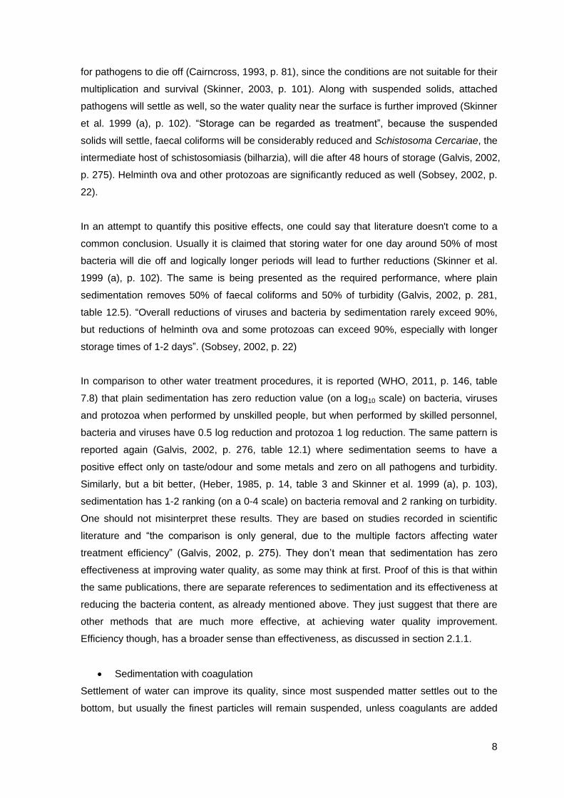
In an attempt to quantify this positive effects, one could say that literature doesn't come to a

common conclusion. Usually it is claimed that storing water for one day around 50% of most

bacteria will die off and logically longer periods will lead to further reductions (Skinner et al.

1999 (a), p. 102). The same is being presented as the required performance, where plain

sedimentation removes 50% of faecal coliforms and 50% of turbidity (Galvis, 2002, p. 281,

table 12.5). “Overall reductions of viruses and bacteria by sedimentation rarely exceed 90%,

but reductions of helminth ova and some protozoas can exceed 90%, especially with longer

storage times of 1-2 days”. (Sobsey, 2002, p. 22)

In comparison to other water treatment procedures, it is reported (WHO, 2011, p. 146, table

7.8) that plain sedimentation has zero reduction value (on a log10 scale) on bacteria, viruses

and protozoa when performed by unskilled people, but when performed by skilled personnel,

bacteria and viruses have 0.5 log reduction and protozoa 1 log reduction. The same pattern is

reported again (Galvis, 2002, p. 276, table 12.1) where sedimentation seems to have a

positive effect only on taste/odour and some metals and zero on all pathogens and turbidity.

Similarly, but a bit better, (Heber, 1985, p. 14, table 3 and Skinner et al. 1999 (a), p. 103),

sedimentation has 1-2 ranking (on a 0-4 scale) on bacteria removal and 2 ranking on turbidity.

One should not misinterpret these results. They are based on studies recorded in scientific

literature and “the comparison is only general, due to the multiple factors affecting water

treatment efficiency” (Galvis, 2002, p. 275). They don’t mean that sedimentation has zero

effectiveness at improving water quality, as some may think at first. Proof of this is that within

the same publications, there are separate references to sedimentation and its effectiveness at

reducing the bacteria content, as already mentioned above. They just suggest that there are

other methods that are much more effective, at achieving water quality improvement.

Efficiency though, has a broader sense than effectiveness, as discussed in section 2.1.1.

Sedimentation with coagulation

Settlement of water can improve its quality, since most suspended matter settles out to the

bottom, but usually the finest particles will remain suspended, unless coagulants are added

9

(Reed et al. 199, p. 47). That argument is based on the fact that density, size and shape of the

particles are crucial to the sedimentation process (Heber, 1985, p. 25 and Davis et al. 2002, p.

318). Particles that are lighter than water will not settle, unless they are attached towards each

other, or towards the added material (Skinner et al. 1999 (b), p. 105), until they become larger.

The added materials are called coagulants.

Basically, coagulants reduce the electrostatic repulsion between particles and allows the

electronic attraction forces (Van der Walls’) to flocculate the particles (Ives, 2002 (b), p. 296).

Common coagulants are reported to be: chemically originated (aluminium sulphate and iron

hydroxide), soil originated (clay and lime), plant originated (moringa seeds and

polysaccharides) (Nath et al. 2006, p. 39). Details on coagulation is beyond the scope of this

project. One may refer to Ken Ives, Coagulation and Flocculation (Ives, 2002 (b)), for further

details.

It is worth mentioning that settlement processes, especially in larger volumes of water,

“seldom perform in accordance with theory”, since the density of water isn’t uniformly

distributed. Moreover, temperature of water and salt content (changing often through

evaporation of water), can alter its density significantly, thus influence the sedimentation

procedure (Heber, 1985, p.29).

All these scientific features in greater detail on the sedimentation process of particles are

again beyond the scope of this literature review. However, the author would recommend the

book of Martin Rhodes, Introduction to Particle Technology, for further understanding.

Basically, sedimentation by gravitational force is ruled by Stoke’ s Law, where the parameters

are: diameter, effective solid density, liquid density, liquid viscosity and settling velocity

(Rhodes, 2008). Shape, population and colloids of particles are also important issues looked

in detail within the chapters of Rhodes’ book. Some of these issues only are presented in

section 2.2.4 within this project.

Sedimentation as pre-treatment

Sedimentation is commonly regarded as initial part of a treatment process, thus called pre-

treatment. It can be either plain sedimentation or sedimentation with coagulation. The

difference now is that it is not regarded as worthy treatment process to be implemented on its

own. “Sedimentation doesn’t remove the harmful organisms, but it helps to clarify the water

before other treatment takes place” (Cairncross, 1993, p. 81)

Usually it is reported that “gravity settling of highly turbid water for household use is

recommended as a pre-treatment for systems that disinfect water with solar radiation, chlorine

10

or other chemical disinfectants” (Sobsey, 2002, p. 23). Turbidity, to put it simply, is less

transparent water, with more flocks in it, within which pathogens may be “protected” (Campbell,

1983, p. 119 and Spellman, 2003, p. 370). Thus chemicals like chlorine or solar radiation

cannot “attack” the harmful pathogens in the water so effectively so larger doses are required.

In that sense, settlement reduces the turbidity and consequently, water demands less chlorine

to be disinfected (Kotlarz et al. 2009) or less solar radiation. Furthermore, settlement of

particles improves practically the aesthetic qualities of water (colour, taste and odour) and

consumers may therefore be more willing to drink it (Sobsey, 2002, p. 23).

The necessity of sedimentation as a pre-treatment method is given in many tables within

publications, even when the writers do not refer to plain sedimentation in their analysis. Tables

like table 3 (Heber, 1985, p. 14) and table 12.4 (Galvis, 2002, p. 280), show clearly that

especially in highly turbid and highly polluted water, plain sedimentation needs to be the initial

step of the treatment process.

Overview of everything on sedimentation is nicely presented in part 4.2: Plain Sedimentation

or Settling, by Sobsey, 2002 (p. 22), where this summary table is taken from.

Table 2.1: Advantages and disadvantages of plain sedimentation for HWT (Source: Sobsey, 2002, p. 22)

Sedimentation can be used on much a bigger scale than that of HWTS, since it is an ancient

method of purification, either when using smaller vessels or even bigger storage tanks

(Sobsey, 2002, p. 22). The Romans were reported to have settling reservoirs within their water

treatment system from 100 AD (Galvis, 2002, p. 271). Publications on water tanks, rainwater

collection systems, waste stabilization ponds, water-wastewater treatment plants and so forth,

always refer on the effectiveness of sedimentation as a crucial part of the treatment process.

Much of the information already presented was based on sedimentation tank design

characteristics (Skinner, 2003, p. 101, Ives, 2002 (a) and Heber, 1985, p 25).

11

2.2 The Three-Pot Water Treatment System

2.2.1 Definition and Background

As mentioned in the above section, the three-pot water treatment system is based both on the

idea of HWTS and on the principle of sedimentation, which are traced back in ancient times

(see sections 2.1.1 and 2.1.3). Searching the literature specifically for the three-pot water

treatment system, it was concluded that the technique was initially launched with this name in

a publication by the International Water and Sanitation Centre (IRC) in 1988 (Smet et al. 1988,

p. 10.13).

The three-pot method is defined within this document to be “an effective means of purification”,

through prolonged storage, where “any type of storage containers can be used” (Smet et al.

1988, p. 10.13). The procedure is serial and basically is the following:

Day 1: Water is collected in pot 1.

Day 2: Water stored for a day in pot 1 is slowly poured in pot 2. Pot 1 is being cleaned and

refilled with raw water.

Day 3: Water stored for a day in pot 2 is slowly poured in pot 3. Pot 2 is being cleaned and

water stored for a day in pot 1 is slowly poured in pot 2. Pot 1 is being cleaned and refilled with

raw water.

Users can consume water from pot 3 on day 3, which has been allowed to settle for 48 hours

or can use the water from pot 3 on day 4, after three days has passed (one day per pot).

Siphoning instead of pouring can be done as well.

Figure 2.1: Prolonged storage (source: Smet et al. 1988, p. 10.13)

12

In chronological order, the three-pot system appeared again in literature in 1999, on a series

of technical briefs by WEDC (Skinner et al. 1999 (a), p. 102). Although the procedure is the

same and the main advantages are described under the “storage and settlement” heading

(see: plain sedimentation in section 2.1.3), the contribution of the particular publication is a

more comprehensive image, including the instructions. One could say that the particular

paper’s significance is that it brought the three-pot more into the scene for HWT. Evidence of

that is the number of publications and websites that started referring to it basically only after

1999 and the fact that the same image is being reproduced in most cases.

Figure 2.2: The three-pot treatment system (source: Skinner et al. 1999 (a), p. 102)

Then the three-pot was roughly mentioned as an alternative water treatment technology under

the “storage and settlement” option in 2000 (CDC, 2000, p. 139). In figures 19 and 20 (CDC,

2000, p. 142-143), there is a comparison table for all HWTS, presenting technical and

economic facts as well. In a publication in 2005, it is shown as a HWT option (Wijk et al. 2005),

along with some advantages and limitations of the method (see section 2.2.2). Also, it was

found again in a 2005 publication, as an option to make safe water for drinking and cooking

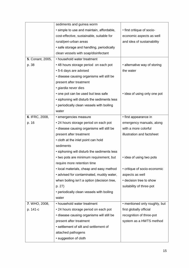
(Conant, 2005, p. 38), where a slightly different idea of the method is introduced. Pots 1 is

being filled with raw water on day 1 and pot 2 on day 2. Water settles for two days in the same

pot, before being poured into pot 3, from which it is directly drinkable. The need for three pots

makes sure that the user has two-day settled water every day, otherwise two pots are enough.

Again the three-pot is cited in 2008, as a method for household water treatment (IFRC, 2008,

p. 16 and 30), but this is the first time it was found to be mentioned as an emergency measure.

A more colorful illustration (p.16) and a factsheet (p. 30) are used this time. The fact that two

instead of three pots can be sufficient with longer retention times is clearly presented as an

“emergency tip”.

13

Figure 2.3: The three-pot method (Source: IFRC, 2008, p. 16)

Although, all publications are respectable and from well known institutions, the most official

recognition one could say, comes with the 3rd

edition of WHO drinking-water guidelines in

2008 (WHO, 2008, p. 141-c), where very roughly the three-pot is described as a simple

sedimentation option for improving drinking-water quality at the household level (WHO

includes the same section in the latest guidelines (WHO, 2011, p. 143) as well). Then it is

more inclusively mentioned in 2010 again as an initial part of the HWTS option (CAWST, 2010,

p. 4), with an attempt to give some more non-technical details (see section 2.2.2 within this

project). In 2011 it was included in WHO technical notes for emergencies once more as part of

the pre-treatment process (Kayaga et al. 2011). The most recent reference to the three-pot

(HETV, 2012 (a)) was on an online update of the (CDC, 2000) publication in 2012, where the

“gap in knowledge” was spotted (see section 2.3).

It is a fact there are quite a few publications and websites referring to the three-pot system, but

most reproduce the above mentioned ones, therefore it is not worth discussing these on this

project. Depicting all the images was done on purpose, so that each time the original

publication can be traced easily.

2.2.2 Overview of Literature on Three-Pot

On this section, a summary table and an overview of the literature found directly on three-pot

system is presented. For review of the “indirect” literature, meaning the sedimentation process,

see section 2.1.3. The publications are in chronological order, the notes are actually what

each publication claims and the last column is the author’s comment.

Publication Notes Comment

1. Smet et al.

1988, p. 10.13

• household water treatment

• 24-48 hours storage period on each pot

• evidence that prolonged storage

improves water quality

• disease causing organisms will still be

present after treatment

• first appearance in official

papers and first illustration

• no reference to that

evidence

14

• settlement of silt and death of pathogens

• siphoning can be used

• safe storage, periodically clean vessels

• no justification why

2. Skinner et al.

1999 (a), p. 102


• 24 hours storage period on each pot

• 50% of most bacteria will die after a day

• longer retention times are better

• cercariae die after 48 hours



• settlement of silt, death of pathogens and

settlement of attached pathogens

• water near the top has better quality

• siphoning will disturb the sediments less


with boiling water

• second appearance that

brings the three-pot in the

scene of HWTS, along with

the most commonly

reproduced illustration

• better explanation on the

removal mechanism

• better justification on

siphoning

3. CDC, 2000, p.

139








• settlement of silt, death of pathogens,

reduction of turbidity

• pots are easily available locally

• no lab tests, no field tests on the method

• cost of three pots only as capital

investment, zero recurrent costs, as long

as the pots last

• basically reproducing

Skinner et al. 1999 (A), p.

102

• mentioning clearly the

turbidity improvement

• first comparison of the

three-pot with the rest HWTS

(figure 19-20, p. 142-143)

• first critique of economic

aspects as well

4. Wijk et al.

2005




• longer retention times can have 90%

reduction



• cloth at the inlet point can hold



102

15

sediments and guinea worm

• simple to use and maintain, affordable,

cost-effective, sustainable, suitable for

rural/peri-urban areas

• safe storage and handling, periodically

clean vessels with soap/disinfectant

• first critique of socio-

economic aspects as well

and idea of sustainability

5. Conant, 2005,

p. 38



• 5-6 days are advised



• giardia never dies

• one pot can be used but less safe


• periodically clean vessels with boiling

water

• alternative way of storing

the water

• idea of using only one pot

6. IFRC, 2008,

p. 16

• emergencies measure




• cloth at the inlet point can hold

sediments


• two pots are minimum requirement, but

require more retention time

• local materials, cheap and easy method

• advised for contaminated, muddy water,

when boiling isn’t a option (decision tree,

p. 27)

• periodically clean vessels with boiling

water

• first appearance in

emergency manuals, along

with a more colorful

illustration and factsheet

• idea of using two pots

• critique of socio-economic

aspects as well

• decision tree to show

suitability of three-pot

7. WHO, 2008,

p. 141-c





• settlement of silt and settlement of

attached pathogens

• suggestion of cloth

• mentioned only roughly, but

first globally official

recognition of three-pot

system as a HWTS method

16

8. CAWST,

2010, p. 4

• initial stage of household water treatment


• longer retention times can have 90%

reduction



• ladling or any gentle-to-the-sediments

method

• lifespan depends on containers

• direct cost practically zero

• simple and easy, therefore robust

• effectiveness tested on the lab, not on

field

• periodically clean vessels with water

• only as part of the overall

household water treatment

• good critique of socio-

economic aspects as well

• using (Sobsey, 2002) as a

reference, but there are no

lab tests on three-pot in that

publication, 90% refer to plain

sedimentation studies

9. Kayaga et al.

2011

• emergencies measure as pre-treatment



• longer retention times are better




• settlement of silt, death of pathogens and

settlement of attached pathogens



with boiling water



102

10. HETV, 2012

(B)








• settlement of silt, death of pathogens,

reduction of turbidity

• pots are easily available locally

• same as (CDC, 2000) only

updated in 2012

17

• no lab tests, no field tests on the method

• cost of three pots only as capital

investment, zero recurrent costs, as long

as the pots last

• there are filed tests, but uncertain if any

lab tests exist

• after the update, field tests

were traced, but not lab ones

Table 2.2: Overview of literature review on the three-pot

As mentioned above, there are several more publications on three-pot, but they all refer or

reproduce the ones summarised on table 2.2. Even among these publications, there is a

tendency to reproduce the first two ones, but still there is a new contribution on each case.

That is how it was decided which publications would be included in the literature review and

which should be left out.

In summary, the three-pot system is mainly described as a HWT option in development and

health publications and is found only in two emergency ones (IFRC, 2008, p. 16 and Kayaga

et al. 2011). The procedure doesn't differ that much on its basis. There are only slight

operational differences, such as: one-two-three pots, pouring-siphoning-ladling water out, 24-

48 hours as retention time, use of cloth for further quality improvement (see section 2.2.3).

Moreover, it is commonly cited that at the end of the treatment period, the pathogens will have

been reduced, but not totally removed. The removal efficiency ranges from 50%-90% and that

percentage varies with different types of pathogens. The magnitude of the effect of these slight

differences remains to be researched (see section 2.3 and chapter 5).

Only relatively recently the idea of overall efficiency of HWTS and not only microbiological

effectiveness started being introduced with the presentation of socio-economic aspects as well.

In (CDC, 2000, p. 143, figure 20), there’s a capital and recurrent cost analysis, where the

three-pot system is claimed not to have costs apart from the initial purchase of the pots (if not

already available). Then in (Wijk et al. 2005), it is suggested that the three-pot is simple to use

and maintain, affordable, cost-effective and therefore sustainable and suitable for rural/peri-

urban areas. Similarly it is presented in (CAWST, 2010, p. 5), where it is characterized as

“robust” instead of “sustainable”.

To summarise the advantages, limitations and ideas on further improvement, table 2.3 was

created. The literature review has also lead to identification of the “gap in knowledge”, as

shown on table 2.2 and explained on section 2.3.

18

Advantages Limitations Further improvement

• both as a regular HWT

option and for emergencies

• disease causing pathogens

are reduced but not eliminated

• use of straining cloth at

the inlet

• pots are easily available at

the local level

• water near the surface is

better than that at the bottom

• siphoning instead of

pouring water

• cheap, basically there’s only

the cost of the pots initially

• improved water after 24-48

hours minimum

• periodically clean vessels

• flexible, any vessel can be

used, 1, 2 or 3 pots as well

• further storage longer

than 48 hours

• simple and easy to use and

maintain

• cost-effective and

sustainable (or robust)

• suitable for rural and peri-

urban communities

Table 2.3: Summary of literature review on the three-pot

2.2.3 Design Characteristics

Figure 2.4: Design characteristics (based on: IFRC, 2008, p. 33)

Studying all the above literature on the three-pot system, the author came up with figure 2.4,

just to depict the design characteristics and to summarise the areas were the publications

have small differences. This idea was conceived after identifying the gap in knowledge (see

section 2.3) and before the laboratory experiments, so as to decide the methodological details

for the experimental procedure (see chapter 3). Similar concept was initially found in previous

thesis as well (Qi, 2007).

The design characteristics are:

1. Inlet

2. Vessel

3. Outlet

19

1. a. Inlet water quality → not specified

b. Inlet water quantity → 2-3 lcd only for drinking in emergencies up to as much is needed

for all the household purposes

c. Use of cloth or not at the inlet point → cloth can filter out larger sediments and guinea

worm

2. a. Size of vessel → not specified, depends on the water quantity

b. Shape of vessel → not specified, depends on availability and preference

c. Material of vessel → not specified in connection to the efficiency (only in (Smet et al.

1988, p. 10.13) earthen potters are better for their cooling effects)

d. Rest vessel characteristics (colour, opening, lid, handle, tap) → not specified (mentioning

only that vessels need to be periodically cleaned)

e. Number of pots in use → three-pots are best, only two-pots are still feasible, one-pot is

possible (but in (Conant, 2005, p. 38) is claimed to be less safe)

f. Retention time (days of storage) → usually 24-48 hours or as long as possible (in (Conant,

2005, p. 38) 5-6 days are claimed to be better) in each vessel or in total

3. a. Method of decanting → pouring, siphoning or ladling

b. Point of abstraction → not specified (in (Skinner et al. 1999 (a), p. 102) suggested better

at the top)

c. Outlet water quality → depends on many variables (usually claimed that there’s 50%

reduction in pathogens after one storage day and up to 90% in total)

For details on the design characteristics and how they may affect the three-pot system, refer

to section 2.4 of the “Related Issues”.

2.2.4 Purification Mechanisms

In the present section, the purification (quality improvement) mechanisms of the three-pot

system is described, based on water/wastewater literature in general. Referring to publications

on sedimentation tanks (LeChevallier et al. 2004, p. 9, table 2.2), the purification processes of

the three-pot system are mainly physical and biological. The rest processes mentioned in the

particular table, basically describe the situation in sedimentation tanks. They can potentially

occur in a pot, but to a smaller extent. In that sense and consulting other literature as well, the

two basic mechanisms are:

1) Physical: a) Transportation of substances

b) Aeration

c) Floatation of substances

2) Biological: Die-off of pathogens

20

It is understood that the main purification processes for the three-pot are sedimentation of

substances and die-off of pathogens. However, the author decided to look at the topic from a

wider perspective and the above larger categories were stated. In similar sense, aeration is

included basically to describe better the case of pouring the water in comparison with

siphoning (see chapter 4) and the use of three pots instead of one. Likewise, floatation will

occur with solids which have lower density than water (Spellman, 2003, p. 545) or are being

held at the surface by the force of buoyancy, as observed during the experiments with small

leaves and insects.

In more detail:

1-a) Transportation

Transportation includes the movement of any type and size of particles that may exist in the

water, organic or inorganic. In recent bibliography, there is a separation between suspended

and colloidal particles. Colloids are sized smaller than 1μm and are dispersed within the water,

so it is more difficult for them to settle on their own (Mara et al. 2003, p. 633). In figure 2.5, one

can see separation techniques for different sized particles. As one notices, bacteria fall under

both categories and viruses are colloidal.

Figure 2.5: Separation techniques for different particle sizes (source: Mara et al. 2003, p. 634)

Either as a suspended particle or as a colloid, in the three-pot case, transportation involves

sedimentation and diffusion (LeChevallier et al. 2004, p. 68), which are also involved in grain

filtration.

21

- Sedimentation occurs when gravity exceeds buoyancy and drag forces on a single particle

(Rhodes, 2008, p. 31). The drag force is basically described by Stoke’ s law which was

proposed in 1851 (Rhodes, 2008, p. 29). That gives a settling velocity UT under gravity :

where: x is the spherical solid’s radius, ρp is the particle’s density, ρf is the fluid’s density, g is

the acceleration due to gravity and μ is the fluid’s viscosity. Shapes other than sphere affect

the basic law (Rhodes, 2008, p. 33). Also, the basic law on a single particle is affected when

there is a multiple particle system, since the motion of each particle is influenced by the motion

of nearby particles (Rhodes, 2008, p. 51). Both of these, apply in the case of settling raw water.

As shown in figure 2.5 or from Stoke’s law, sedimentation is more effective when the particle is

bigger.

- Diffusion is ruled by Brown’s movement law and thermal energy. According to this, random

motion increases the contact probability between particles and thermal energy (translated into

water temperature) increases these random collisions (Rhodes, 2008, p. 119).

In cases of grain filtering, authors refer to attachment or adsorption, separately to

transportation, as a purification mechanism. Applying the idea of adsorption can be used in the

three-pot case, in order to explain the attachment of suspended particles to one another and

the formation of colloids. The forces that rule both transportation and attachment, besides

Stoke’s and Brown’s mentioned above (body forces), are Coulomb and van der Walls (surface

forces) (Huisman et al. 1974, p.30). Surface forces contribute to transportation before any

contact is made (Huisman et al. 1974, p.30) and in the case of colloids, they play an even

more significant role than the body forces (Rhodes, 2008., p. 117).

- Mass attraction is ruled by van der Walls forces. It is the universal attraction force for atoms

and molecules basically, therefore it applies when particles are in proximity (Mara et al. 2003,

p. 635).

- Electric interaction is ruled by Coulomb forces. It is actually attractive or repellent forces,

between same or opposite charged surface layers (single or double layers) (Mara et al. 2003,

p. 635). Organic colloids, including bacteria are usually negatively charged, therefore they are

most likely to be repelled by one another (Huisman et al. 1974, p.30).

There is also the DLVO theory, that looks at these two surface forces in combination and

predicts the stability of colloids, depending on particles separation distance and salt

concentration (Mara et al. 2003, p. 637). One interesting point to note is that based on

22

coagulation kinetics theories (Mara et al. 2003, p. 642), collision of particles occur better in

turbulent flow and the higher the particle concentration, the better. For details on colloids in

general, one may refer to chapter 38: Coagulation and filtration in (Mara et al. 2003) or chapter

5: Colloids and fine particles in (Rhodes, 2008).

To sum up, many variables will affect the transportation mechanism, so it is difficult to predict

every time the effectiveness based on theoretical models. These variables are: particle size

and shape, particle density, particle surface charge, liquid density, liquid viscosity, liquid

temperature, salt content, settling velocity, particles population, colloids, turbulence.

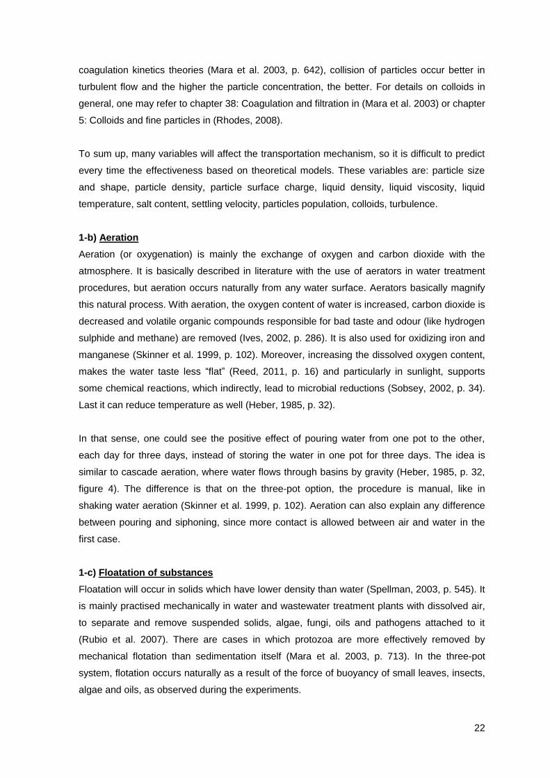
1-b) Aeration

Aeration (or oxygenation) is mainly the exchange of oxygen and carbon dioxide with the

atmosphere. It is basically described in literature with the use of aerators in water treatment

procedures, but aeration occurs naturally from any water surface. Aerators basically magnify

this natural process. With aeration, the oxygen content of water is increased, carbon dioxide is

decreased and volatile organic compounds responsible for bad taste and odour (like hydrogen

sulphide and methane) are removed (Ives, 2002, p. 286). It is also used for oxidizing iron and

manganese (Skinner et al. 1999, p. 102). Moreover, increasing the dissolved oxygen content,

makes the water taste less “flat” (Reed, 2011, p. 16) and particularly in sunlight, supports

some chemical reactions, which indirectly, lead to microbial reductions (Sobsey, 2002, p. 34).

Last it can reduce temperature as well (Heber, 1985, p. 32).

In that sense, one could see the positive effect of pouring water from one pot to the other,

each day for three days, instead of storing the water in one pot for three days. The idea is

similar to cascade aeration, where water flows through basins by gravity (Heber, 1985, p. 32,

figure 4). The difference is that on the three-pot option, the procedure is manual, like in

shaking water aeration (Skinner et al. 1999, p. 102). Aeration can also explain any difference

between pouring and siphoning, since more contact is allowed between air and water in the

first case.

1-c) Floatation of substances

Floatation will occur in solids which have lower density than water (Spellman, 2003, p. 545). It

is mainly practised mechanically in water and wastewater treatment plants with dissolved air,

to separate and remove suspended solids, algae, fungi, oils and pathogens attached to it

(Rubio et al. 2007). There are cases in which protozoa are more effectively removed by

mechanical flotation than sedimentation itself (Mara et al. 2003, p. 713). In the three-pot

system, flotation occurs naturally as a result of the force of buoyancy of small leaves, insects,

algae and oils, as observed during the experiments.

23

2) Die-off of pathogens

Reduction of pathogens in the three-pot system is mainly due to their sedimentation (alone or

adsorbed to suspended solids) and natural die-off. Death in nature may occur by aging, by

starvation or by predation by other organisms (Mara et al. 2003, p. 486). The ability to survive

is called persistence (Feachem et al. 1983, p.59).

Aging is part of the natural growth cycle, as shown in figure 2.6. The environmental conditions

(oxygen, pH, temperature, nutrients, toxicity) prolong or speed up the natural death procedure

(Spellman, 2003, p. 329).

Figure 2.6: Micro-organism growth curve (source: Spellman, 2003, p. 329)

Starvation is when there is not enough food for pathogens to grow and multiply. Organic food

in a closed system (like the pot) will decrease in quantity as time goes by. Food is being

consumed by pathogens continuously, but logically some of it is being adsorbed by suspended

solids as well. This actually raises natural competition between pathogens (Huisman et al.

1974, p.22) and only the most persistent will be able to survive. Predation is when certain

organisms are using other pathogens as their food, as it is reported in some cases (Mara et al.

2003, p. 616).

“For any given system, there are essentially two factors in pathogen removal: how long the

pathogen stays in the system and how quickly it dies” (Mara et al. 2003, p. 482 and Feachem

et al. 1983, p. 59). In other words, retention time and type of pathogen, affect the above curve

or natural death, besides the environmental conditions. Based on experiments, die-off kinetics

of pathogens are based on first order equations, so they follow an exponential curve, which is

basically the last part of the whole growth cycle. Reproduced in all literature from (Feachem et

al. 1983, p. 207):

or

24

where: C is the concentration of pathogens at T time, T is time, k is the die-off rate and Co is

the concentration at T=0. Death rates are higher in natural water, with active flora and fauna,

and increase with the rise of temperature (Feachem et al. 1983, p. 209). According to that

theory, the probability of a pathogen dying is independent of its age. But practical studies,

show evidence of multiplication or even recovery (Mara et al. 2003, p. 617). This is of limited

duration and occurs in specific nutrient, temperature and non-competitive environments

(Feachem et al. 1983, p. 209). This is logical to happen, since it is actually the initial stage of

the growth curve in figure 2.6. In a limited environment though, where the conditions are stable

and there is no active treatment, but with time allowed to pass, passive treatment is being

applied in a natural way (Strauss, 1985, p. 4). This is called the “self-purification” process of

water bodies (Mara et al. 2003, p. 616).

The last theory worth to mention is borrowed from die-off kinetics in ponds, reproduced form

(Marais, 1974). For a single pond:

where: Ne is the number of bacteria per unit of effluent volume, Ni likewise for influent volume,

Θ is the mean hydraulic retention time in days and Kt is a constant depending on temperature.

From observations, for temperatures 5-20 oC, Kt=2.6*1.19

(T-20), where T is temperature. For a

series a ponds with the same retention time, that equation would become:

where: n is the number of ponds and Θp the mean hydraulic retention time in each pond. As a

result of multiple ponds in series, water quality is further improved, than when one single pond

is used. This is basically because short-circuiting and its resulting turbulence are being

minimized, therefore sedimentation is aided (Mara et al. 2003, p. 487 and LeChevallier et al.

2004, p.9). It would be interesting to see if that mathematical model can be applied in the case

of three-pots instead of three-ponds.

2.3 Gaps in Knowledge

2.3.1 Absence of laboratory experiments

In an attempt to find and compare studies on the HWT methods, (CDC, 2000) on p. 142, figure

19, states that there are no lab, nor field tests on “storage and settlement”, translated as the

three-pot system in this case. However, an updated version of this figure was found on-line

(HETV, 2012 (b)). Of course since 2000 that the original CDC handbook was published,

research on HWT options has thrived, as they have gained more recognition. So on the

updated figure, it is stated that there are field tests on the three-pot system, but there’s

25

uncertainty if there are any lab tests, since they didn't seem to be able to trace any. Therefore

the question mark in the relevant column (see figure 2.5). This gap in knowledge resulting

form lack of laboratory testing is what the present project is attempting to cover.

System Process Removal Lab

tests

Field

tests Advantages Constraints

Figure 2.7: Gap in knowledge (based on: HETV, 2012 (b))

The fact that the table was updated after 2000, therefore it is assumed to be correct, was

double checked by looking at the rest HWT options mentioned. Characteristically, the slow

sand filters and the rapid sand filters were both stated not to have lab/field tests on the 2000

version, but later, the updated 2012 version, stated correctly that lab/field tests exist.

2.3.2 Gaps in Knowledge

Once the initial gap in knowledge was traced, the specific objectives of the lab research

needed to be decided. By looking at the design characteristics (section 2.2.3), it became clear

that there were plenty of variables that could be tested. A robust laboratory test usually keeps

all the variables constant, except the one that is under examination (see chapter 3). The

author, with the valuable guidance of the supervisor, decided that it is worth focusing on

testing the information found in literature, that is not properly justified, but keeps on being

reproduced. That were considered to the more specific gaps in knowledge.

Publication referring to the removal effectiveness of pathogens on the three-pot

system, usually claim a 50% bacteria reduction for one day storage and up to 90% with longer

retention times (see table 2.2). The source of this information was traced in literature about

sedimentation (see plain sedimentation part of section 2.1.3). As mentioned above, since the

three-pot system, only recently started to be looked at separately, most publications reproduce

one another. Usually (Skinner et al. 1999 (a), p. 102) is being reproduced on publications that

claim the 50% reduction and that publication was not based on any experimental work. Only

after (Sobsey, 2002) presented the up-to-90% reduction (p.22) in his section on plain

sedimentation, some later publications on the three-pot referred to that percentage (Wijk et al.

2005 and CAWST, 2010, p. 4). These two publications refer to Sobsey for that 90% figure.

26

The point is that Sobsey has reviewed previously existing literature to write his report. As a

result these numbers are based on research done on plain sedimentation and not on the three

pot system in particular. One doesn’t claim that the general rules of sedimentation do not

apply in this case, but since there are so many variables involved in settlement itself, it would

be worth for one to research the subject of sedimentation on such a small scale. In that sense,

the researcher decided to examine the reduction efficiency for bacteria using the three-pot

system.

The small scale of the three-pot is probably one of the reasons why there hasn’t been much

research done on the topic, according to author’s opinion, since there are plenty of

publications on sedimentation, waste stabilization ponds, storage tanks etc., which are large

scale systems. Also testing the effectiveness of such a simple and small scale system may

seem not worth for an institution to spend its time and resources on. Last, it is interesting that

almost all HWT options, give a chance to institutions and companies to launch new products in

the market. Research have always been reported to go along with the market demands. The

three-pot system on the other hand, consisting of any three containers available, doesn't give

many opportunities for market expansion, thus research may not be promoted for it. Important

fact to note is that the only HWT option which managed to be recognised and was scaled up

without dealing with market terms was solar disinfection, known by the name SODIS.

For the other gaps in knowledge, it wasn’t possible to trace the initial literature they were

based on, like for the effectiveness on bacteria removal. Looking at table 2.2 and section 2.2.3,

the researcher identified points not properly justified that can be seen as possible features to

investigate through experimentation.

The factor that changes more within the three-pot literature is the retention time,

starting from 24 hours, until 6 days. It is commonly said that longer retention times lead to

further improvement, but it would be interesting to examine that particular argument.

Another thing not properly justified is the use of siphoning instead of pouring. Most

literature mentions that the sediments will be less disturbed, but again it would be interesting

to examine if actually the use of a siphon affects the effectiveness of the three-pot system.

Another point of difference is the use of 1-2-3 pots. As mentioned above, three-pots

are advised, two-pots are considered as minimum, but even with one pot the treatment may

work, although not advised. The idea of comparing the three-pot results to the one-stable pot

results is worth testing.

27

Last, it is stated that water near the surface is of better quality than that near the

bottom of the pot. By taking samples from both points one may be able to test if there is

actually a difference and hence understand better the purification mechanism, in particular for

the three-pot.

2.4 Related Issues

The related issues are variables that are inevitably connected to the three-pot system and they

are worth to mention, since they had an impact on research methodology as well.

2.4.1 Water Quantity

Water is undeniably connected with survival, health, well-being and development. “An

adequate amount of safe water is necessary to prevent death from dehydration, to reduce the

risk of water-related disease and to provide for consumption, cooking and personal and

domestic hygienic requirements” (Sphere, 2011, p. 83). Apart from health, when “water

availability is poor, people will loose time, energy or money, that could have been invested

elsewhere” (Rottier et al. 2003, p. 52).

The uses of water are many, but there is an hierarchy on the needs that people cover with

them (Reed, 2005, p. 2, figure 1). Domestic water, including water for drinking, food

preparation, laundry, personal and domestic hygiene (WHO, 2011, p. 83), is the most

essential for everyday life, therefore is hierarchically higher. Within that part, drinking water is

the minimum requirement for preserving life, thus it’s on the top of all. Drinking water is the

amount the body needs to compensate for losses of respiration perspiration, urination and

defecation (Howard et al. 2003, p. 4).

The water quantity each person needs per day (lcd=litres/capita/day), is something depending

in many factors like: cultural, socio-economic status, hygiene awareness, productive uses of

water, cost, quality, effort, distance from source and so forth (Howard et al. 2003, p. 17 and

Nozaic, 2002, p, 62). For drinking water, it depends on individual physiology, sex, age, climate,

food and work load (Howard et al. 2003, chapter 3, p. 3).

Literature on emergencies looks at the aspect of minimum requirement of water, as well as

quantities needed in normal conditions. There are small differences about lcd, depending on

what each publication defines as “basic survival needs”. In general, it is agreed that 3-5 lcd are

needed for survival immediately after a disaster (drinking and cooking only, with no use for

hygiene included), 15 lcd as an intermediate supply measure (hygiene included) and 20-50 lcd

in normal conditions of development (DeVeer, 2002, p. 538, table 24.1). Many other

28

publications refer to the number of 7.5 lcd, as the basic survival quantity, including very basic

hygiene (Sphere, 2011, p. 98), since that number is sufficient for most people, under most

conditions (WHO, 2011, p. 83). Referring only to drinking water, the minimum quantity of

intake, excluding water indirectly consumed through food, for an average adult in average

conditions, that is 2 lcd (Howard et al. 2003, p. 6 and WHO, 2011, p. 83).

In cases of emergency or where the availability of good quality water is not large, it is advised

that people should treat at least their drinking water, if there is no other option (Skinner et al.

1999, p. 101). Apart from looking how much water each person needs, one should consider

how many people there are in the household as well (Reed, 2005, p. 1). In that sense,

accepting that people need on average 2 lcd water for drinking, for an average household size

of five people, the absolute minimum requirement would be 10 l/day. This fact, along with the

fact that in the local market of Loughborough there were no other sized pots with lids for safe

storage, led to the use of 10 l pots for the experiments. This is a manageable weight for a

single person to lift for pouring the water out. For larger containers, two people or the use of a

siphon is likely to be required.

2.4.2 Water Quality

Water quality is undeniably connected with health. Parameters in order to determine and

measure quality are categorized similarly in different publications. More officially (WHO, 2011),

the categories are: microbial, chemical, radiological and acceptability issues. One may refer to

chapters 7, 8, 9 and 10 in (WHO, 2011) for details. The principal concern in water remains the

microbiological quality, since it is related to many common diseases (Howard, 2002 p. 10).

Water-related diseases are those where water helps or hinders the transmission of

communicable diseases (DFID, 1998, p. 63). The classification of transmission mechanisms to:

water-borne / water-washed / water-based / water-related is widely used, adopted from

(Cairncross et al. 1993, p. 4), is widely used. Pathogens are the micro-organisms that are

responsible for the diseases. Most common pathogens are: viruses, bacteria, protozoa,

helminths (worms), rickettsiae and fungi (Rottier et al. 2003, p. 9). In (Cairncross et al. 1993, p.

10, table 1.2) one can find examples of these pathogens and which diseases they are

responsible for, according to the above classification. Figure 2.8, gives a quick description on

some of them. For further detail, one may refer to (Mara et al. 2003), chapters 2, 3 and 4.

29

Figure 2.8: Some water-related pathogens (source: NWP, 2010, p. 11)

In studies reviewing contamination of drinking water with pathogens, conclude that the

majority of those which are of main concern, are excreta related (Ashbolt, 2004, p. 231). This

means that they are spread by pathogens principally found in human faeces and are

transmitted by the faecal-oral route (Howard, 2002 p. 4). It is far too complex to detect all the

harmful pathogens in water, therefore tests look for indicator bacteria (Cairncross, 1993). Their

presence/absence indicates faecal contamination and therefore, there is a probability that

other pathogens may be present as well (Pickford, 1991, p. 73). In that sense, the absence of

these indicators should characterize water as low risk, rather than as safe (Howard, 2002, p.

12).

Looking at the characteristics that a pathogen should have in order to become an indicator

(Howard, 2002 p. 12, box 2), it is difficult to find one ideal organism to cover them all (Mara et

al. p. 105). The closest match are the thermotolerant (faecal) coliform bacteria. These are a

sub-group of the total coliform group. Total coliform bacteria (that grow at 37 oC) include non-

faecal bacteria as well, thus they are not ideal indicator for faecal pollution. On the contrary,

thermotolerant (faecal) coliform bacteria (that grow at 44 oC) nearly always indicate faecal

contamination. Usually, 95% of the thermotolerant bacteria are the Escherichia coli (E. coli)

that is always found in the gut of warm-blooded animals (Bartram et al. 1996, p. 10.2).

Therefore, E. coli is widely used as an indicator bacterium for faecal pollution in most tests

and in the present project as well. E. coli is further subdivided in six types (Hunter, 2003). All

types cause diarrhoea, with different severity, but the most common type met worldwide is the

Enterotoxigenic E. coli (ETEC).

Apart from E. coli, which is the typical microbial parameter checked in water quality tests,

other common parameters, which will be tested in this project are: temperature, colour,

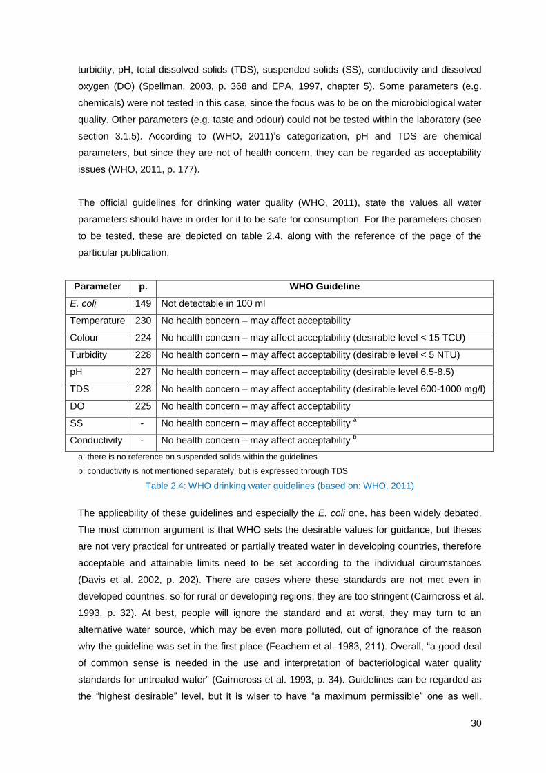
30

turbidity, pH, total dissolved solids (TDS), suspended solids (SS), conductivity and dissolved

oxygen (DO) (Spellman, 2003, p. 368 and EPA, 1997, chapter 5). Some parameters (e.g.

chemicals) were not tested in this case, since the focus was to be on the microbiological water

quality. Other parameters (e.g. taste and odour) could not be tested within the laboratory (see

section 3.1.5). According to (WHO, 2011)’s categorization, pH and TDS are chemical

parameters, but since they are not of health concern, they can be regarded as acceptability

issues (WHO, 2011, p. 177).

The official guidelines for drinking water quality (WHO, 2011), state the values all water

parameters should have in order for it to be safe for consumption. For the parameters chosen

to be tested, these are depicted on table 2.4, along with the reference of the page of the

particular publication.

Parameter p. WHO Guideline

E. coli 149 Not detectable in 100 ml

Temperature 230 No health concern – may affect acceptability

Colour 224 No health concern – may affect acceptability (desirable level < 15 TCU)

Turbidity 228 No health concern – may affect acceptability (desirable level < 5 NTU)

pH 227 No health concern – may affect acceptability (desirable level 6.5-8.5)

TDS 228 No health concern – may affect acceptability (desirable level 600-1000 mg/l)

DO 225 No health concern – may affect acceptability

SS - No health concern – may affect acceptability a

Conductivity - No health concern – may affect acceptability b

a: there is no reference on suspended solids within the guidelines

b: conductivity is not mentioned separately, but is expressed through TDS

Table 2.4: WHO drinking water guidelines (based on: WHO, 2011)

The applicability of these guidelines and especially the E. coli one, has been widely debated.

The most common argument is that WHO sets the desirable values for guidance, but theses

are not very practical for untreated or partially treated water in developing countries, therefore

acceptable and attainable limits need to be set according to the individual circumstances

(Davis et al. 2002, p. 202). There are cases where these standards are not met even in

developed countries, so for rural or developing regions, they are too stringent (Cairncross et al.

1993, p. 32). At best, people will ignore the standard and at worst, they may turn to an

alternative water source, which may be even more polluted, out of ignorance of the reason

why the guideline was set in the first place (Feachem et al. 1983, 211). Overall, “a good deal

of common sense is needed in the use and interpretation of bacteriological water quality

standards for untreated water” (Cairncross et al. 1993, p. 34). Guidelines can be regarded as

the “highest desirable” level, but it is wiser to have “a maximum permissible” one as well.

31

Interim improvements should be incrementally leading from the “permissible” to the desirable

one (Nozaic, 2002, p 68).

WHO suggests zero faecal coliforms in any 100 ml sample of drinking water, since the

guidelines are formed for life-long consumption of water. But this doesn't mean that people

cannot survive if they ingest some numbers of faecal coliforms. “Many healthy farming families

in the UK regularly drink water with tens if not hundreds of faecal coliforms per 100 ml”

(Cairncross, 1993). That raises the issue of “infectious dose” or when water can be

characterized as safe. Infectious dose is when a sufficient number of pathogens has been

ingested, so the disease occurs (Mara et al. 2003, p 58). It is commonly reported as ID50

(median Infectious Dose), meaning the number of organisms that infects 50% of the

individuals. This number varies among pathogens and different people. Indeed for E. coli, for

the commonest type-ETEC this can be 108-10

10 organisms, while for EHEC

(Enterohaemorrhagic) 100-106 (Hunter, 2003, p. 67-68).

The idea of infectious dose interpreted as safety, gives a classification of risks within the

publications, for faecal coliforms or E. coli in particular, as shown in table 2.5. The

classification is the same either in development or emergency manuals. Only in (WHO and

UNICEF, 2005) there is a classification (table 3, p. 27) that characterizes contaminated water

differently according to the population. The smaller the population (e.g. rural places) the less

strict the standards are for a supply to be acceptable. This is logical according to the law of

probabilities, one may comment, but very theoretical to be practiced safely. Note that this risk

categorization refers only to E. coli and doesn’t include the risk of having other pathogens

present in the water.

Count

(per 100 ml)

Risk category

(Nozaic, 2002, p. 69)

Inference

(House et al. 1999, p. 79)

Action

(Harvey, 2007)

0 Conformity with WHO Reasonable quality may be consumed as it is

1-10 Low risk Reasonable quality may be consumed as it is

11-100 Intermediate risk Polluted treat if possible but may be

consumed untreated

101-1000 High risk Dangerous must be treated

>1000 Very high risk Very dangerous reject or treat heavily

Table 2.5: Risk classification for E. coli in water supplies

Again there is a debate on whether WHO guideline for zero coliforms is suitable in each case.

That limit is said to be pointless for developing countries (Feachem et al. 1983, p. 211), for

rural areas or emergencies (Nath et al. 2006, p. 35), where more flexibility is required. Others,

suggest no more than 10 faecal coliforms/100ml (Davis et al. 2002, p. 202). A moderately

good quality can even be <100 faecal coliforms/100 ml (Feachem et al. 1983, p. 210).

Combining all the above details, the threshold in the present project, for water quality to be

32

characterized polluted and must be treated, was decided to be 1000 faecal coliforms/100 ml

(see chapter 3 for how this affects the methodology). Interesting point to mention is that any

classification and process, needs to be regularly checked, since all pathogens tend to evolve

(Ashbolt, 2004, p. 236).

The principle one could say behind all that, is the idea of “improvement” and how each

publication perceives it. That can be improvement strictly on water quality or improvement to a

person’s life linked to water. Improvement of water quality is lowering the numbers of

pathogens to an acceptable level and not necessarily eliminating them – this is sterilization

(Spellman, 2003, p. 314). “ A moderately effective water treatment that raises the levels of the

most important quality parameters – those that affect health – without meeting all the

parameters and standards” may be perceived as an improvement in water quality (Heber,

1985, p. 13). When people use 1000 faecal coliform/100 ml drinking water, a treatment that

provides 50 faecal coliform/100 ml, is already a major improvement (Feachem et al. 1983, p.

211).

Improvement to a person’s life linked to water is a broader concept. When it comes to a

general health outcome, it is described officially (WHO, 2011, p. 38), with disability adjusted

life years (DALY). “In many parts of the world, the implementation of a water quality

intervention that results in an estimated health gain of more than 5% would be considered

extremely worthwhile” (WHO, 2011, p. 136). The improvement also has to do with water

affecting important aspects of living, like child mortality, school attendance, equity, productivity

and so forth (WHO and UNICEF, 2005, p. 10). Diseases related to water and poor health, are

expensive in money, time and energy and hinder development at a personal and national level

(Rottier et al. 2003, p. 44).

Improvement, in any case, needs to be progressive, with realistic goals between the

incremental steps (WHO and UNICEF, 2005, p. 27). With the narrow or the broader

perspective and with the strict or more flexible guidelines, any water treatment intervention, is

crucial for the overall improvement of people’s lives and should be regarded as an extra

contribution to that difficult goal. A water treatment intervention that improves water quality

should not be eliminated, just because it doesn't meet some standards from the beginning.

2.4.3 Water quantity versus water quality

A number of factors play an important role in interrupting the transmission of diseases. The

most commonly mentioned are water, sanitation and hygiene (Pickford, 1991, p. 69). More

specifically, crucial aspects are: water quantity, water quality, education, vector control,

excreta disposal and water management (Pickford, 1991, p. 77). Publications debate

33

significantly, over the importance of water quality versus water quantity. An attempt to review

the literature on the topic, was included in section 2.1.2, when looking at the point-of-use and

household water treatment options, since these claim that quality is more important after all.

Good review of this debate or the shifting in the HWTS paradigm as often referred, can be

found in a short version in (Clasen, 2005). To summarise here, initially quality was regarded

more significant, but around 1990, due to Esrey’s research, quantity appeared to have a

greater effect than quality, but also that good hygiene and sanitation have even greater

impacts (House et al. 1999, p. 80, table 6). Only around 2000, researchers started to question

this fact, since HWTS appeared to be twice as effective to traditional source-based

interventions, but the HWTS interventions were never reviewed within Esrey’s work (Clasen,

2009, p. 54).

Other publications, do not take side in this debate, but more wisely claim that: “the relative

importance of water quality and water quantity depends on the situation” (House et al. 1999, p.

80). In emergencies for example, it is usually stated that “until minimum standards for both

water quantity and quality are met, the priority is to provide equitable access to an adequate

quantity of water even if it is of intermediate quality” (Sphere, 2011, p. 98).

In a similar sense one may comment, that overall, it is not a matter of “versus”, but a matter of

“and”. Since there doesn't seem to be a clear conclusion out of all these arguments about the

“versus”, one could see the positive side of all this research and say that quality “and” quantity,

always play some positive role. “In spite of doubts about the detail, it is clear that such

environmental interventions can have a substantial effect... We know enough to do a lot...”

(Cairncross et al. 2010, p. 203).

2.4.4 Issues related to the design characteristics

On this section there is a review on the literature that affected the design characteristics (as

summarised in section 2.2.3) of the experiments. Using the same order as before:

1. a. Inlet water quality

As explained in section 2.4.2, the threshold for one to consider the water so polluted that

needs treatment was decided to be 1000 faecal coliforms/100ml. This is a commonly found

concentration for E. coli in surface waters, as reported in publications (for example, streams in

developing countries (Cairncross et al. 1993, p. 33, table 3.1) may have up to 10000 E.

coliI/100ml). The selection of surface water and the particular loading of bacteria is described

in chapter 3.

34

1. b. Inlet water quantity

As explained in section 2.4.1, 10 litres of water will be used, as the amount of water treated by

each three-pot system.

1. c. Use of cloth or not at the inlet point

Cloth filtration is reported to have advantages in water filtration, especially by trapping solids,

helmiths (like guinea worm) and cholera virus. Since the effectiveness depends on the cloth as

well, use of a cloth use would introduce many new variables, that couldn’t be tested at this

point and the focus should remain on the three-pot system. Thus no cloth was used.

2. a. Size of vessel

As explained in page section 2.4.1, according to the quantity and the availability of containers

with lid in Loughborough, 10 litres vessels will be used. These are in accordance with water

collection standards as well (see 2.e: number of pots).

2. b. Shape of vessel

Shape was decided to be cylindrical, that of a typical household bucket. Buckets are easily

available everywhere, and the user can collect, transport, treat (in the three-pot case), store

and consume water from the same vessel easily (Reed, 2011). They are also stackable and

they don’t have edges to concentrate the water load, thus become worn out more quickly

(Reed, 2011, p. 6). The absence of corners don't facilitate the bacteria colonies to grow as well

(Oxfam, 2008, p. 4). Besides, there weren’t many other options in the market either.

2. c. Material of vessel

The containers available in the market were mainly plastic. Plastic can be used in this case,

since it is commonly found everywhere and people choose it, since it is light, durable, strong

and cheap (Reed, 2011, p. 11). Also, the aim was to use an inactive material, so as not to

affect the bacteria removal. Different materials are reported to alter the water parameters like

pH, turbidity, conductivity, TDS and therefore the bacteria die-off rates (Qi, 2007) or even the

chlorine required for water treatment (Ogutu et al. 2001). Plastic is relatively inactive in

producing salts and altering pH (Ensslin, 2005), so its effect on bacteria removal is considered

minimal.

2. d. Rest vessel characteristics (colour, opening, lid, handle, tap)

The colour was intentionally light, so that one could inspect the suspended solids gathering at

the bottom. If the buckets are placed somewhere with sun exposure, transparent or

translucent materials could promote algae growth, if regular cleaning does not take place. The

opening needs to be wide enough, for water to be poured in and out without spillages and

35

wastages (Reed, 2011, p. 10), but also for the container to be cleaned easily (Reed, 2011, p.

18). Containers with a tight lid were chosen, so as to promote safe storage and prevent re-

contamination (Reed, 2011, p. 13). Handles assist carrying the container and may assist with

pouring the water as well, but do not affect the experiments. Last, since the idea was to test

pouring and siphoning, tap use was irrelevant in this case. As mentioned before, 10 litres

weight is manageable when pouring water out. In larger volumes, siphoning or other decanting

methods may have to be used.

2. e. Number of pots in use

There are water collection standards, which claim that “two vessels of 10-20 litres for

collecting water, plus one 20 litres vessel for water storage, per 5 person household” is ideal

for emergencies (Reed, 2005, p. 3). Alternatively, this is an interim measure, since for

emergencies one 10-20 litres container is enough (DeVeer, 2002, p. 538, table 24.1). Taking

that into consideration, along with the facts on the three-pot literature (three containers are

best, with two it’s still feasible and with one is possible, but maybe less safe), the researcher

decided to use three-pots in comparison with one-pot (see 2.3.2: gaps in knowledge).

2. f. Retention time (days of storage)

Within the literature for three-pot , retention time was from 24 hours, until 6 days, with longer

retention times claimed to lead to further improvement. One may refer to section 2.2.4 on die-

off of pathogens for more details on retention time.

3. a. Method of decanting

The three-pot options were pouring, siphoning or ladling. Pouring is simple, but is difficult to do

with large filled containers (Reed, 2011, p. 13) and it may lead to wastages. Siphoning can be

used to overcome the weight lifting issue, but regular cleaning of the siphon needs to be done,

so as not to pollute the water, when it is dipped into it. Ladling the water with a dipper is simple

and easy, but it raises the risk of recontamination again, if the users are not aware of hygiene

issues (Reed, 2011, p. 13) and it is a slow process as well. In this case, the researcher

decided to compare pouring and siphoning (see 2.3.2: gaps in knowledge).

3. b. Point of abstraction

For the three-pot, it is stated that water near the surface is of better quality than near the

bottom. By taking samples from both points the researcher will test if there is actually a

difference, in order to conclude on whether bacteria settle and/or die, as part of the purification

mechanism.

36

3. c. Outlet water quality

The parameters to be checked, as explained in section 2.4.2, are E. coli, temperature, colour,

turbidity, pH, total dissolved solids (TDS), suspended solids (SS), conductivity and dissolved

oxygen (DO). There should be a comparison with WHO guidelines (table 2.4), but as

commented before, these values cannot be the only argument against or in favor of any

treatment method. In (DeVeer, 2002, p. 538, table 24.1) one may find different values,

depending on emergency, interim or development cases, but also in (Novaic, 2002, p. 71,

table 4.8 and p. 72, table 4.9) there are different standards depending on the country of origin.

37

3.0 Methodology

The present chapter explains how the research was planned and how the experiments were

conducted in order to answer the research questions and meet the objectives.

3.1 Planning Procedure

3.1.1 Overview

The aim of the project is to test the effectiveness of the three-pot water treatment system.

Thorough literature review was conducted in order to understand the issues related to the

three-pot system and identify particular gaps in knowledge (see section 2.3.2). That led to the

formation of five research questions. By answering these, the aim of the project can be

addressed more specifically. The research questions are:






In order to answer these questions, experiments A and B were conducted (see section 3.2). In

summary, experiment A was conducted in three trials with different raw water quality for each

one. The typical three-pot system procedure, were water is allowed to settle one day per each

pot, before being decanted, was followed. Three containers in series were used within each

three-day time period. Water was poured and siphoned in parallel three-pot systems.

Experiment B was conducted in two trials, again with different raw water quality for each. Two

pots were used in rotation within a period of 7 days. Water was poured after being allowed to

settle for a day. Experiment A addressed specifically question 3, experiment B addressed

specifically question 4 and both of them addressed questions 1, 2 and 5.

Data for the measured parameters were collected in Excel sheets (see appendices 8.1 and

8.2). Excel was used to create all the tables and graphs within this project. In order to conduct

proper analysis, literature research was repeated to address more specific questions. For the

shake of triangulation, results from similar tests in previous researches were attempted to be

found. With a minor exception (see section 4.2.1), no similar research was found. The three-

pot system is an area where laboratory experiments haven’t been conducted yet, as presented

in section 2.3.1.

38

3.1.2 Water source

The laboratory experiments were aimed to be conducted in as realistic conditions as possible.

For that reason, water needed to be transferred from a natural surface source. Adjacent to

WEDC, there are two brooks, Holywell and Burleigh, shown on the map. They were both

accessible and nearby Sir Frank Gibb Laboratories of the Civil and Building Engineering

Department of Loughborough University (lab on the map), were the experiments were to be

held. The final choice would be based on the E. coli loading of each brook. As mentioned in

section 2.4.2, within this project, the threshold for a water sample to be characterized as

contaminated, was chosen to be 1000 cfu/100 ml.

Figure 3.1: Map of WEDC area, showing the water source location (adopted from: http://maps.lboro.ac.uk/)

From the literature review, two previous thesis were found were the same choice between the

brooks needed to be made. In (Huang, 2006), various water sources near WEDC were

sampled. The particular author, took samples only one day of August within his project, so his

results were not perceived that representative for the brooks. However, in (Thye, 2007), more

samples were taken within the experimental period (July-August). It is stated that the two

brooks didn't differ that much around that period of time, but Holywell was chosen for

accessibility reasons. Last, laboratory keeps annual records for Holywell brook contamination.

Reviewing these, the average concentration of E. coli was 1410-1820 cfu/100 ml.

Since bacteria concentrations vary within a year due to several factors, it was wiser to conduct

trial tests prior to the actual experiments, in order to have a clear picture of the two brooks,

WEDC

lab Burleigh

Holywell

2

39

thus finalise the choice. The exact locations are the ones shown on the map for Burleigh and

Holywell brooks. Burleigh was accessible only at the particular point, due to absence of

blocking vegetation. Holywell on the other hand was accessible at more locations. Location no.

2, was an additional abstraction point for Holywell brook with wider banks, thus more stagnant

water. It was intentionally chosen to see if that would make any difference to the water quality.

See appendix 8.4 for the results of testing these three locations. These trial tests were

conducted with the valuable help of Mrs. Jayshree Bhuptani, Deputy School Superintendent,

Analytical Chemist and Supervisor of the laboratory, as a teaching session for all the

experimental procedures.

As shown in appendix 8.4, the first location had 890 cfu/100 ml, which was closer to the 1000

cfu/100 ml threshold. Burleigh had 580 cfu/100 ml, which was quite lower, therefore that brook

was not opted. The second location in Holywell brook, where the water was more stagnant,

had 770 cfu/100 ml, although only about 20 meters away from the first location. The banks

were wider and water was moving slower, but also the water level dropped. That is actually

the evidence that sedimentation is a natural self-purification process of water bodies. As

mentioned in (Mara et al. p. 616), rivers usually contain higher levels of bacteria than lakes,

because of the sorter residence time of water in rivers, therefore the self-purification process

has less time to effect. Along with pathogens, suspended solids have more time to settle as

well, which brings down the levels of turbidity and colour. This is shown in the results of

appendix 8.4. Dissolved oxygen on the other hand is a bit higher in the second location, again

as expected. The level of water is lower and air can pass through the water column more

easily. The final point of abstraction from Holywell brook, pointed in the map under the name

“Holywell”, is shown in reality in figure 3.2.

Figure 3.2: Point of abstraction in Holywell brook (author, 2012)

40

3.1.3 Water collection and transportation

Prior to any collection and laboratory experiments, a risk assessment was conducted by the

author and approved from the laboratory department. For the experiments, water collection

was done manually with the aid of a hand trolley. A laboratory water group technician, Mr.

Geoffrey Russell, was providing his valuable help in this task every time. Water was

abstracted directly with a 10 l bucket from the brook and was being decanted in a 100 l

container, shown in figure 3.3. This amount was sufficient to fill the first pot from all three-pot

systems tested each time. Collection was done every morning at 9:00 pm, in an attempt to

have similar temperature for all raw water. The container was covered during transportation, to

avoid spillages and recontamination. Safety precautions were followed according to the risk

assessment guidance to minimize the hazards associated to the task.

Figure 3.3: Water collection and transportation (author, 2012)

Water was then decanted with the aid of the 10 l bucket into the first pot of each three-pot

system within the laboratory. It was understood that while water was transferred, some

settlement of suspended solids and bacteria might have occurred. For this reason, water was

stirred thoroughly with the aid of a wooden stick, before it was decanted in the lab, in an

attempt to re-suspend the settled matter. Despite stirring up the water, there was still the

concern of having different quality within the water column of the 100 l container. The aim was

to have similar initial quality in all three-pot systems for them to be comparable. For that

reason the first pots were not filled in series. Instead, every time a 10 l bucket was abstracting

water from the 100 l container, all pots were filled with some amount of this water. That way

the first pots were filled gradually, with water evenly abstracted through the 100 l water column.

3.1.4 Water sampling

Water was sampled with the a 100 ml scaled glass syringe from each pot. In total 125 ml were

needed in order to test all the parameters (see section 3.1.5) and placed in 125 ml bottles.

41

Suitable labels were placed on the bottles to avoid mixing up the samples. All samples of raw

water were analysed as soon as possible, to ensure that the real conditions were captured.

Moreover, the typical three-pot system procedure is about allowing water to settle for 24 hours

before decanting each time. Therefore, all the rest samples apart from the raw water were

analysed around the same time every day. That would ensure that water would have been

allowed to settle approximately for 24 hours before analysis each day, thus safeguarding that

the three-pot system procedure was followed.

The syringe was the optimum decision for sampling water from the pots in this case, since it

caused almost no disturbance to the water and its suspended matter. It had a long and very

thin needle able to touch the bottom of the container, thus allow measurements at any depth.

Alternatively, a pipette could be used, but when immersed into the water, it trapped a small

amount of water while moving along. For measurements from a specific point, that would be

problematic, since the water sampled wouldn't necessarily come from that point. Another

option was to place small horizontal tubes with some kind of a tap, coming out of the container,

to take the measurements from each point. There was the concern though that sediments and

bacteria would settle on the tube’s edges, thus these measurements might be higher than the

actual ones within the rest of the container. As a result a removable equipment like the syringe

was opted.

The syringe was sampling water from the same point within each container, so as to have

comparable measurements. When only one sample from each container was taken, the

syringe was placed at the middle height and at the centre of the circular bottom. That gave a

middle-centred measurement, which was assumed to be representative for the whole

container. When points from other heights were to be sampled (surface or bottom), the syringe

was placed again at the centre of the circular shape, but at the appropriate height at each

case. Bottom measurements were conducted with the syringe touching the bottom, to be able

to sample the microscopic bacteria, if present.

3.1.5 Testing parameters and equipment

The parameters to be tested within this project, as mentioned in section 2.4.2 as well, were: E.

coli, temperature, colour, turbidity, pH, total dissolved solids (TDS), suspended solids (SS),

conductivity and dissolved oxygen (DO) (Spellman, 2003, p. 368 and EPA, 1997, chapter 5).

Each parameter’s brief description follows:

E. coli is a type of bacterium. It belongs to the thermotolerant (faecal) coliform bacteria

group. This is a sub-group of the total coliform group. They grow at 44 oC. Usually, 95% of the

thermotolerant bacteria are the Escherichia coli (E. coli), found in the guts of warm-blooded

42

animals (Bartram et al. 1996, p. 10.2). Therefore, E. coli is widely used as an indicator

bacterium for faecal pollution in most tests and in the present project as well. E. coli is further

subdivided in six types (Hunter, 2003). They all cause diarrhoea, with different severity, but the

most common type met worldwide is the Enterotoxigenic E. coli (ETEC). Within this project, E.

coli is measured in cfu/100 ml.

Temperature is a physical property of water, quantifying the amount of heat enclosed

within it. It is not usually an evaluating factor for water, but it affects many other biological and

chemical processes (EPA, 1997, p. 147), like the solubility of oxygen, the rate of bacterial

activity and the rate at which other gases are transferred to and from the water (Spellman,

2003, p. 372). Ambient temperature (i.e.: temperature of the surrounding environment) has the

most profound effect on shallow surface water (Spellman, 2003, p. 373). Within this project, it

is measured in oC.

Colour is a physical characteristic of water. While pure water is colorless, natural water

takes on color from foreign substances like organic matter, vegetation, minerals, various

microorganisms and wastes (Spellman, 2003, p. 371). Color is classified as true and apparent.

Color contributed by suspended solids is characterized apparent. True color is the result of

dissolved chemicals that cannot be seen and is separated from apparent color by filtering the

water (Spellman, 2003, p. 299). Color is not necessarily a problem, but it affects acceptability

and it may be an indication of pollution. Within this project, colour is measured in Hazen. True

Colour Units (TCU), can be used only for true color, after filtration.

Turbidity is a measure of water clarity and is caused by the presence of suspended

matter, which decrease the passage of light through the water. Suspended materials include

soil particles (clay, silt, and sand), algae, plankton, microbes, and other substances. Turbidity

can affect the color of the water, thus acceptability. Higher turbidity can increase the water

temperatures because suspended particles absorb more heat. This in turn, can reduce the

concentration of dissolved oxygen, because warm water holds less dissolved oxygen than

cold (EPA, 1997, p. 154). Also, the colloidal matter associated with turbidity provides

absorption sites for microorganisms that may be harmful or cause undesirable taste and odour

(Spellman, 2003, p. 370). Within this project, turbidity is measured in NTU.

pH is used to indicate how acidic or basic a substance is. It is actually a measurement

of the hydrogen ions (H+) concentration. More H

+ result to an acidic substance, therefore a low

pH, while less H+ or more OH

-, result to a basic substance, therefore to a high pH. pH is

important to the chemical reactions within the water and too low or too high values can inhibit

43

the growth of microorganisms (Spellman, 2003, p. 300). pH is measured with the scale of 0-14

pH units.

Total dissolved solids (TDS) are part of the total solids within water. They are mainly

minerals, salts, metals, anions and cations dissolved in water, which still remain in water after

filtration. They can be both organic and inorganic. Too low or too high concentrations result in

unacceptable taste (Spellman, 2003, p. 373). Within this project, TDS are measured in ppm.

Suspended solids (SS) are part of the total solids within water. SS include silt and clay

particles, plankton, algae, fine organic debris and other particulate matter, which can be

trapped by a filter. SS can act as carriers for pathogens and substances attached to them.

They also affect the turbidity and colour levels, thus affecting acceptability as well (EPA, 1997,

p. 176. Within this project, SS are measured in mg/l.

Conductivity is a measure of the ability of water to pass an electrical current. It is

affected by the amount of inorganic anions and cations in water. Moreover, it is affected by

temperature, with warmer waters rising the conductivity. (Spellman, 2003, p. 420). Basically,

attachment of inorganic matter with the settled solids, can significantly reduce conductivity.

Also, there is a connection with TDS and pH since these are partly or totally anions and

cations too. Within this project, conductivity is measured in μS/cm.

Dissolved oxygen (DO) is the oxygen within the water. Since it is a gas, its solubility in

water depends on the water temperature, when the pressure is the atmospheric one. The

higher the temperature, the lower the saturation level of the gas (Spellman, 2003, p. 299).

Oxygen is exchanged between water and the atmosphere through its surface. It can be

consumed and/or produced within the water body, depending on the biological activity of the

organisms present in the water (EPA, 1997, p. 139). Within this project, DO is measured in

mg/l.

The equipment used to test each parameter, along with the procedure were according to

standard operational methods. For each parameter, a brief description follows:

E. coli were measured with the Membrane Filter for members of the Coliform group

(MFC) standard procedure. Initially, 3,7 gr of broth were added to 100 ml of distilled water in a

conical flask. After proper mixing of those two elements, 1 ml of rosolic acid was added as well.

The conical flask was placed for approximately 1,5 minutes in the microwave oven at

maximum temperature, until small bubbles immerged from the liquid (beginning of boiling

point). That solution was left to come in room temperature, within a bath of tap water. In the

44

meantime, the sterile Petri dishes (50 mm) were placed in order for proper labeling according

to the samples. A sterile nutrient pad was added in each Petri dish. With a sterilized pipette,

2,5 ml of the broth solution was placed onto the pad, to create the nutrient conditions for the

bacteria to grow. The specific nutrient assists the growth of thermotolerant (faecal) coliforms in

particular, thus it was chosen. Since 95% of the thermotolerant bacteria are E. coli, the

bacteria growing onto the pad were considered to be E. coli as well. In that sense, within this

project, when the author refers to E. coli counts, it is actually thermotolerant counts.

Figure 3.4: Labeled Petri Dishes in series and in detail (author, 2012)

Once the dishes were ready, the membrane filtration procedure could begin. A sterile Nalgen

filter holder with receiver was used. A membrane filter cellulose paper (white, gridded with

0.45 μm pore size) was picked from its sterile pack with lab forceps and placed onto the holder.

The forceps were sterilized each time above fire. In 225 ml of ringer’s solution (i.e.: isotonic

solution of water with several salts, similar to the bodily liquids), 25 ml of the water sample was

added and mixed properly. That gives a ratio between them of 1/10 or 10-1

dilution, as usually

called. Then, 50 ml of this solution was added on the upper part of the membrane kit and

vacuumed manually into the receiver. The filter was then picked up and placed carefully on top

of the nutrient pad in the Petri dish, avoiding capturing air bubbles. Once all the filters were

placed in their dishes, they were placed in the 44 oC incubator for 18-24 hours.

Figure 3.5: Nalgen filter holder with receiver (author, 2012)

After that period has passed, the E. coli formed blue colonies. With a magnifier they were

counted one by one. Since the filtered water was 50 ml, that number was multiplied by 2, to be

converted into cfu per 100 ml. That number was then multiplied by 10, since it was 10-1

diluted,

so as finally to be expressed into cfu/100 ml. It is always advised to incubate two samples

http://en.wikipedia.org/wiki/Isotonic_solutions

http://en.wikipedia.org/wiki/Isotonic_solutions

45

minimum for each E. coli measurement one wishes to take and use their mean value. This

way the result is double-checked and thus not random. In general, if there is time and

resources, three-five samples are the best option. In experiment A, three measurements were

taken (MLSB a-b-c in appendix 8.1), whereas in experiment B, due to limited resources only

two measurements were taken (MLSB a-b in appendix 8.2).

In the trial testing prior to the experiments, done as training session, the typical field

Membrane Lauryl Sulphate Broth (MLSB) filtration procedure was practiced as well. The field

kits normally use Sulphate Broth medium as a nutrient for the bacteria. With that, the exact

same procedure is followed, but the initial medium is prepared with 52 gr of it in 1 l of distilled

water. This produces yellowish E. coli colonies. The MLSB medium was not opted because it

produced less distinct and clear colonies, making them less easy to count. Also, as shown in

appendix 8.4 for MFC and MLSB measurements in the trial testing, the MLSB method

produced less consistent results between the two measurements (a-b) which were taken for

reliability reasons, while the MFC method was found more reliable and could be trusted. (To

avoid confusion, note that in the appendices MLSB is mistakenly written where MFC is

supposed to be and the other way around).

Figure 3.6: Petri dish with blue distinct colonies after MLSB medium (author, 2012)

Temperature was measured with a Digital High Temperature 8’’ lab thermometer in oC.

The probe was placed in the sample for sufficient time, until the indication in the screen

stabilized. The ambient temperature was measured by the typical mercury-glass thermometer

placed in the laboratory wall.

Figure 3.7: Digital High Temperature 8’’ lab thermometer (author, 2012)

Colour was measured with the Siemens Photometer P15 in Hazen units. 10 ml of

distilled water were initially placed in the plastic tube to calibrate the equipment for zero colour

units. Then 10 ml of the actual water to be tested were taken with a syringe from the sample

bottles and placed in the photometer’s tube. The digital screen displayed the units. The tubes

were cleaned after every use with distilled water.

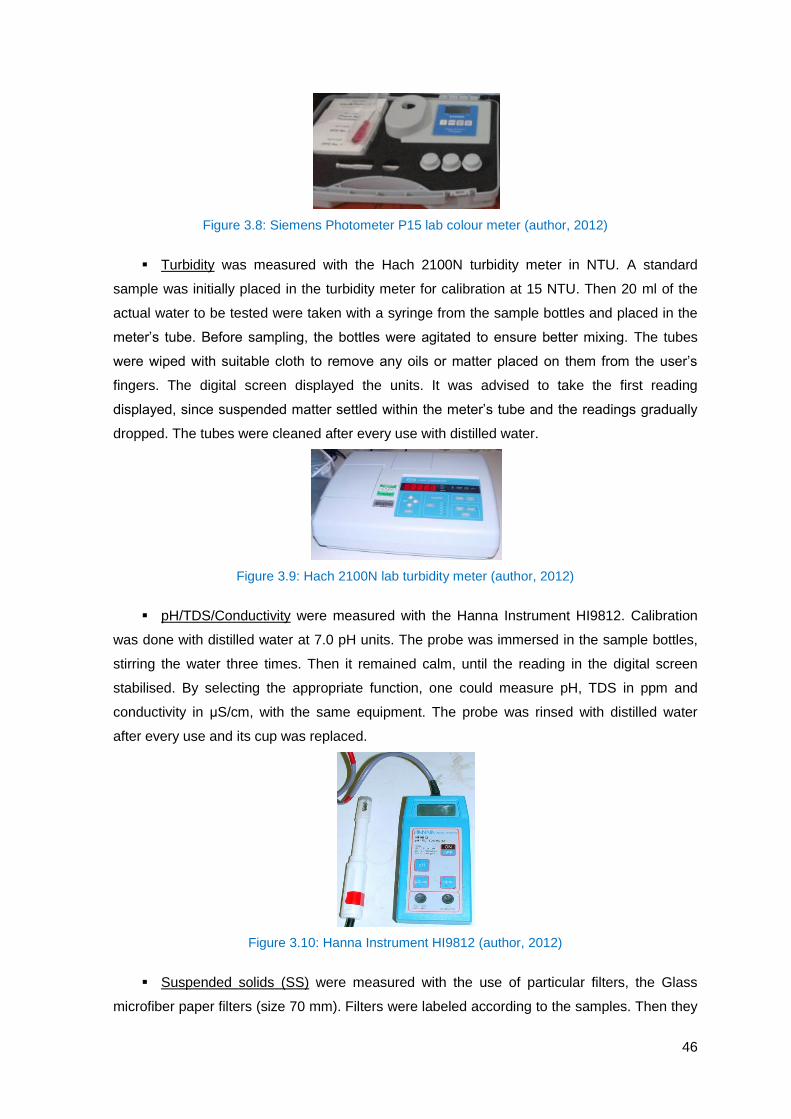
46

Figure 3.8: Siemens Photometer P15 lab colour meter (author, 2012)

Turbidity was measured with the Hach 2100N turbidity meter in NTU. A standard

sample was initially placed in the turbidity meter for calibration at 15 NTU. Then 20 ml of the

actual water to be tested were taken with a syringe from the sample bottles and placed in the

meter’s tube. Before sampling, the bottles were agitated to ensure better mixing. The tubes

were wiped with suitable cloth to remove any oils or matter placed on them from the user’s

fingers. The digital screen displayed the units. It was advised to take the first reading

displayed, since suspended matter settled within the meter’s tube and the readings gradually

dropped. The tubes were cleaned after every use with distilled water.

Figure 3.9: Hach 2100N lab turbidity meter (author, 2012)

pH/TDS/Conductivity were measured with the Hanna Instrument HI9812. Calibration

was done with distilled water at 7.0 pH units. The probe was immersed in the sample bottles,

stirring the water three times. Then it remained calm, until the reading in the digital screen

stabilised. By selecting the appropriate function, one could measure pH, TDS in ppm and

conductivity in μS/cm, with the same equipment. The probe was rinsed with distilled water

after every use and its cup was replaced.

Figure 3.10: Hanna Instrument HI9812 (author, 2012)

Suspended solids (SS) were measured with the use of particular filters, the Glass

microfiber paper filters (size 70 mm). Filters were labeled according to the samples. Then they

47

were weighted in a digital scale, after the scale was calibrated at zero weight. The

measurements were recorded. Then the filters were placed onto a filtering flask and 100 ml of

the sample bottles were measured and poured over the filters. A small electric suction pump

connected to the filtering flask assisted the filtering process. When all the water was filtered,

the filters were removed and placed in the 105 oC oven for 1 hour. After taken out of the oven,

they were let to cool down in room temperature for about 15 minutes, in a small chamber were

atmospheric humidity was absorbed by special gravel placed at the bottom of the chamber.

Last the filters were weighted again on the scale and records of the measurements were taken.

The increase in weight gave the suspended solids loading. As recorded in the raw data excel

sheets in the appendices, the used filter weight minus the clean filter weight, gives the

suspended solids in gr/100 ml. These numbers were very small, thus changed into mg/l

(gr/ml*10000=mg/l) for the final record.

Figure 3.11: Suspended solids Glass microfiber paper filters in use (author, 2012)

Note that all filters were handled with laboratory forceps, throughout the process, so as to

avoid dirt and oils from the user’s fingers to be deposited on the filters. These would add up to

the weight of the suspended solids and the measurements wouldn't represent the actual

suspended solids loading of the water. Moreover, in case the suspended solids filter pack has

been opened in advance, the filters tended to gather humidity from the atmosphere. As a

result in their first weighting procedure, the humidity increased the actual weight of the filter,

without the user realizing that. After water was filtered through the paper and the filters were

placed in the oven, humidity was evaporating along with the water. When the filters were

weighted for a second time, they were found to be less heavy than before, despite the

suspended solids loading. That was because the humidity was not present any more within

the filter. These readings produced false results. It was wiser then, if better quality filters which

do not absorb humidity that easily are not available, to pre-wet the paper filters with distilled

water, following the same filtering procedure, using the flask and the small pump. Then the

filters can be placed in the oven for at least an hour. Alternatively, they can remain there for

long, until the time to be used arrives. That safeguards that the humidity from the air is no

longer present and that the filters are not given another chance to re-absorb it.

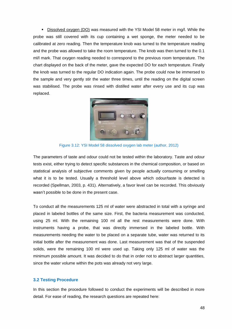
48

Dissolved oxygen (DO) was measured with the YSI Model 58 meter in mg/l. While the

probe was still covered with its cup containing a wet sponge, the meter needed to be

calibrated at zero reading. Then the temperature knob was turned to the temperature reading

and the probe was allowed to take the room temperature. The knob was then turned to the 0.1

ml/l mark. That oxygen reading needed to correspond to the previous room temperature. The

chart displayed on the back of the meter, gave the expected DO for each temperature. Finally

the knob was turned to the regular DO indication again. The probe could now be immersed to

the sample and very gently stir the water three times, until the reading on the digital screen

was stabilised. The probe was rinsed with distilled water after every use and its cup was

replaced.

Figure 3.12: YSI Model 58 dissolved oxygen lab meter (author, 2012)

The parameters of taste and odour could not be tested within the laboratory. Taste and odour

tests exist, either trying to detect specific substances in the chemical composition, or based on

statistical analysis of subjective comments given by people actually consuming or smelling

what it is to be tested. Usually a threshold level above which odour/taste is detected is

recorded (Spellman, 2003, p. 431). Alternatively, a favor level can be recorded. This obviously

wasn’t possible to be done in the present case.

To conduct all the measurements 125 ml of water were abstracted in total with a syringe and

placed in labeled bottles of the same size. First, the bacteria measurement was conducted,

using 25 ml. With the remaining 100 ml all the rest measurements were done. With

instruments having a probe, that was directly immersed in the labeled bottle. With

measurements needing the water to be placed on a separate tube, water was returned to its

initial bottle after the measurement was done. Last measurement was that of the suspended

solids, were the remaining 100 ml were used up. Taking only 125 ml of water was the

minimum possible amount. It was decided to do that in order not to abstract larger quantities,

since the water volume within the pots was already not very large.

3.2 Testing Procedure

In this section the procedure followed to conduct the experiments will be described in more

detail. For ease of reading, the research questions are repeated here:

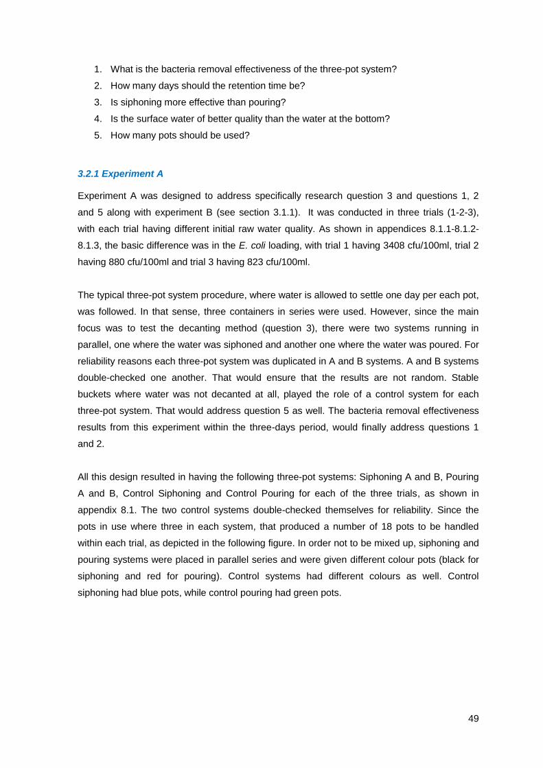
49






3.2.1 Experiment A

Experiment A was designed to address specifically research question 3 and questions 1, 2

and 5 along with experiment B (see section 3.1.1). It was conducted in three trials (1-2-3),

with each trial having different initial raw water quality. As shown in appendices 8.1.1-8.1.2-

8.1.3, the basic difference was in the E. coli loading, with trial 1 having 3408 cfu/100ml, trial 2

having 880 cfu/100ml and trial 3 having 823 cfu/100ml.

The typical three-pot system procedure, where water is allowed to settle one day per each pot,

was followed. In that sense, three containers in series were used. However, since the main

focus was to test the decanting method (question 3), there were two systems running in

parallel, one where the water was siphoned and another one where the water was poured. For

reliability reasons each three-pot system was duplicated in A and B systems. A and B systems

double-checked one another. That would ensure that the results are not random. Stable

buckets where water was not decanted at all, played the role of a control system for each

three-pot system. That would address question 5 as well. The bacteria removal effectiveness

results from this experiment within the three-days period, would finally address questions 1

and 2.

All this design resulted in having the following three-pot systems: Siphoning A and B, Pouring

A and B, Control Siphoning and Control Pouring for each of the three trials, as shown in

appendix 8.1. The two control systems double-checked themselves for reliability. Since the

pots in use where three in each system, that produced a number of 18 pots to be handled

within each trial, as depicted in the following figure. In order not to be mixed up, siphoning and

pouring systems were placed in parallel series and were given different colour pots (black for

siphoning and red for pouring). Control systems had different colours as well. Control

siphoning had blue pots, while control pouring had green pots.

50

Figure 3.13: Experimental setup: Pouring systems in red (right front side) – Siphoning systems in black (left front side) – Control pouring systems in green (right back side) – Control siphoning

systems in blue (left back side) (author, 2012)

Moreover, proper labeling was given to the pots and distinctive arrows and lines were drawn to

separate the systems and indicate the order of decanting, as shown in figure 3.14. Prior to

placement, right after the purchase of the pots, each container was checked for cracks by

being filled with tap water and then calibrated from 0.5-10 litres, to be easier to distinguish the

volume of water within each pot.

Figure 3.14: Labels, distinctive lines and arrows separating the three-pot systems marked in the picture (author, 2012)

Every morning at the same time, water was being decanted to the next container. All the

measurements were done on samples from the water that was being transferred into the new

pot to see any improvement on the quality after one day of storage. The only measurement

that was done both before and after the water was decanted was the dissolved oxygen one.

That was done in an attempt to see the effect of aeration in the treatment process, compared

especially between the siphoning and pouring systems. Every time the water was decanted,

the left volume of water was thrown away, in such a way that it would carry along all the

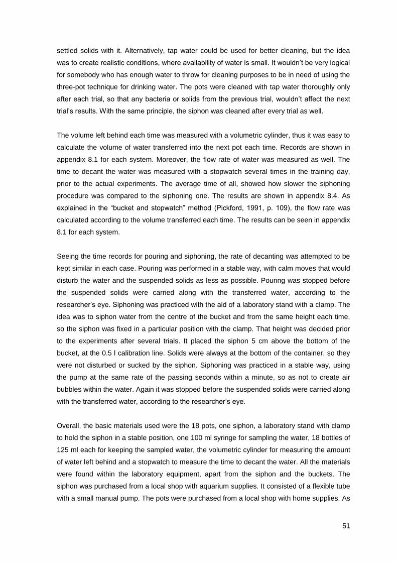
51

settled solids with it. Alternatively, tap water could be used for better cleaning, but the idea

was to create realistic conditions, where availability of water is small. It wouldn’t be very logical

for somebody who has enough water to throw for cleaning purposes to be in need of using the

three-pot technique for drinking water. The pots were cleaned with tap water thoroughly only

after each trial, so that any bacteria or solids from the previous trial, wouldn’t affect the next

trial’s results. With the same principle, the siphon was cleaned after every trial as well.

The volume left behind each time was measured with a volumetric cylinder, thus it was easy to

calculate the volume of water transferred into the next pot each time. Records are shown in

appendix 8.1 for each system. Moreover, the flow rate of water was measured as well. The

time to decant the water was measured with a stopwatch several times in the training day,

prior to the actual experiments. The average time of all, showed how slower the siphoning

procedure was compared to the siphoning one. The results are shown in appendix 8.4. As

explained in the “bucket and stopwatch” method (Pickford, 1991, p. 109), the flow rate was

calculated according to the volume transferred each time. The results can be seen in appendix

8.1 for each system.

Seeing the time records for pouring and siphoning, the rate of decanting was attempted to be

kept similar in each case. Pouring was performed in a stable way, with calm moves that would

disturb the water and the suspended solids as less as possible. Pouring was stopped before

the suspended solids were carried along with the transferred water, according to the

researcher’s eye. Siphoning was practiced with the aid of a laboratory stand with a clamp. The

idea was to siphon water from the centre of the bucket and from the same height each time,

so the siphon was fixed in a particular position with the clamp. That height was decided prior

to the experiments after several trials. It placed the siphon 5 cm above the bottom of the

bucket, at the 0.5 l calibration line. Solids were always at the bottom of the container, so they

were not disturbed or sucked by the siphon. Siphoning was practiced in a stable way, using

the pump at the same rate of the passing seconds within a minute, so as not to create air

bubbles within the water. Again it was stopped before the suspended solids were carried along

with the transferred water, according to the researcher’s eye.

Overall, the basic materials used were the 18 pots, one siphon, a laboratory stand with clamp

to hold the siphon in a stable position, one 100 ml syringe for sampling the water, 18 bottles of

125 ml each for keeping the sampled water, the volumetric cylinder for measuring the amount

of water left behind and a stopwatch to measure the time to decant the water. All the materials

were found within the laboratory equipment, apart from the siphon and the buckets. The

siphon was purchased from a local shop with aquarium supplies. It consisted of a flexible tube

with a small manual pump. The pots were purchased from a local shop with home supplies. As

52

explained in section 2.4.1, 10 l pots were decided to be used. Besides, there were no other

sized pots with a fit lid for safe storage in the local market of Loughborough.

Figure 3.15: Siphon used for the experiments (author, 2012)

3.2.2. Experiment B

Experiment B was designed to address specifically research question 4 and questions 1, 2

and 5, along with experiment A (see 3.1.1). It was conducted in two trials (1-2), with each trial

having different initial raw water quality. As shown in appendices 8.2.1-8.2.2, their only

difference was in the E. coli loading, with trial 1 having 8780 cfu/100ml and trial 2 having

17400 cfu/100ml.

In this case, the typical three-pot system procedure, where water is allowed to settle one day

per each pot, was not followed. Instead, 7 days were decided to be the retention time. That

would address research question 2. Two containers were used this time in rotation, so as not

to have 7 pots in series. Since siphoning and pouring didn't seem to have much difference

from experiment A, in experiment B only pouring was practiced, since it was a lot quicker.

Water was poured after being allowed to settle for a day. Trial 1 and 2 experiments were

conducted in parallel. For reliability reasons each 7-day system was duplicated in A and B

systems. A and B systems double-checked one another. That would ensure that the results

are not random. Stable buckets were water was not decanted at all, played the role of a

control system for each 7-day system. That would address question 5 as well. The bacteria

removal effectiveness from this experiment would address question 1. Moreover,

measurements were taken from the water transferred into the next pot and from the water left

behind. That would address research question 4.

All this design resulted in having the following 7-day systems: “9000” A and B, “17000” A and

B, Control “9000” and Control “17000”. The numbers indicate the rounded-up figure of E. coli.

For each system, “transferred” water and “left” water measurements were taken, while in the

case of the control systems, these were converted into surface and bottom measurements, in

order to be comparable with the decanted water ones. Raw data for these systems are shown

in appendix 8.2. Since the pots in use where two in each system, that produced a number of 8

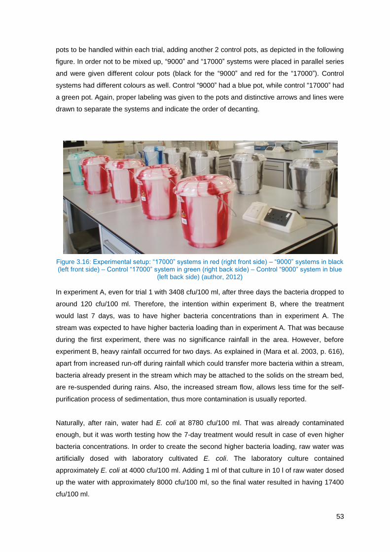
53

pots to be handled within each trial, adding another 2 control pots, as depicted in the following

figure. In order not to be mixed up, “9000” and “17000” systems were placed in parallel series

and were given different colour pots (black for the “9000” and red for the “17000”). Control

systems had different colours as well. Control “9000” had a blue pot, while control “17000” had

a green pot. Again, proper labeling was given to the pots and distinctive arrows and lines were

drawn to separate the systems and indicate the order of decanting.

Figure 3.16: Experimental setup: “17000” systems in red (right front side) – “9000” systems in black (left front side) – Control “17000” system in green (right back side) – Control “9000” system in blue

(left back side) (author, 2012)

In experiment A, even for trial 1 with 3408 cfu/100 ml, after three days the bacteria dropped to

around 120 cfu/100 ml. Therefore, the intention within experiment B, where the treatment

would last 7 days, was to have higher bacteria concentrations than in experiment A. The

stream was expected to have higher bacteria loading than in experiment A. That was because

during the first experiment, there was no significance rainfall in the area. However, before

experiment B, heavy rainfall occurred for two days. As explained in (Mara et al. 2003, p. 616),

apart from increased run-off during rainfall which could transfer more bacteria within a stream,

bacteria already present in the stream which may be attached to the solids on the stream bed,

are re-suspended during rains. Also, the increased stream flow, allows less time for the self-

purification process of sedimentation, thus more contamination is usually reported.

Naturally, after rain, water had E. coli at 8780 cfu/100 ml. That was already contaminated

enough, but it was worth testing how the 7-day treatment would result in case of even higher

bacteria concentrations. In order to create the second higher bacteria loading, raw water was

artificially dosed with laboratory cultivated E. coli. The laboratory culture contained

approximately E. coli at 4000 cfu/100 ml. Adding 1 ml of that culture in 10 l of raw water dosed

up the water with approximately 8000 cfu/100 ml, so the final water resulted in having 17400

cfu/100 ml.

54

The procedure for experiment B, was similar to that of experiment A, thus here described in

summary. Every morning at the same time, water was poured to the next container.

Measurements were done both on the water transferred into the next container and on the

water left behind. That was done in an attempt to see if there is a difference in quality,

between surface and bottom water. Every time the water was decanted, the left volume of

water was thrown away after being sampled, in such a way that it would carry along all the

settled solids with it. Pouring was performed in a stable way, with calm moves that would

disturb the water and the suspended solids as less as possible. This time, instead of relying on

eyesight, standard volume was left behind for all systems. That was initially 1 l to ensure that

no suspended solids were transferred. After two days that most of the visible suspended solids

were not present any more, that volume became 0.5 l. If that change wasn’t done, the water

for treatment after 7 days would be only 3 litres, while it started with 10 l. Records are shown

in appendix 8.2 for each system.

3.2.3 Unexpected conditions

Some unexpected conditions appeared during the experiments. After two days of proper use,

one of the containers developed a tiny hole at the bottom, through which water was leaking

out. Fortunately, it was spotted immediately and not much water was wasted. One of the

empty pots was used, until the hole was filled with silicon and left to dry. The problem didn't re-

appear.

Another issue was the flotation of oils on the water surface to a very small extent in some pots

in experiment A. There was the concern that this could be the initial stage of a biofilm

formation (i.e. surface attached matrix composed of micro-organisms), with E. coli floating

instead of settling. Fortunately, this was not the case. One may refer to section 4.1.3 for

further details.

The issue with the suspended solids filters gathering humidity, thus producing false results,

mentioned in section 3.1.5, was one of the major unexpected limitations of the project. This

couldn't be foreseen and avoided. It emerged in experiment A and it was made sure that it

wouldn't occur again in experiment B, by pre-wetting the filters.

Another limitation occurred when the syringe was abstracting water from the bottom of the

containers. The syringe was always placed in the centre of the circular bottom of the pot, to

produce comparable results from all pots. However, this proved to be faulty, because the

syringe was gradually clearing the particular spot each day by sucking 100 ml out. This was

noticed from the suspended solids which “disappeared” from the centre of the pot. Therefore,

these results could not be trusted (see section 4.2.4). Alternatively, the syringe could abstract

55

water form a different point each time, but then one could claim that the measurements are not

comparable.

Last limitation occurred when water was sampled from the middle-centre of the vessel. Since

the syringe was handled manually, the point of abstraction wasn’t kept steady while the

syringe was used. So these measurements were a bit more random, one may say. In some

cases where the results are not uniform, with no obvious explanation, this random effect is

assumed to be the cause.

56

4.0 Results and Analysis

This chapter presents the laboratory results of the experimental work of the project. The

graphs of the measured parameters are shown, along with comments and observations.

Detailed Excel sheets of the graph data are presented in the appendices. Then the analysis in

the form of discussion follows, where the results are compared with existing theories and

standards. Limitations of the author’s work are stated in the last section, with suggestions for

future improvement.

4.1 Lab Results

In order to answer the research questions, experiments A and B were conducted (see section

3.2). In summary, experiment A was conducted in three trials with different raw water quality

for each one. The typical three-pot system procedure, were water is allowed to settle one day

per each pot, before being decanted, was followed. Three containers in series were used

within each three-day time period. Water was poured and siphoned in parallel three-pot

systems. Experiment B was conducted in two trials, again with different raw water quality for

each. Two pots were used in rotation within a period of 7 days. Water was poured after being

allowed to settle for a day. Experiment A addressed specifically question 3, experiment B

addressed specifically question 4 and both of them addressed questions 1, 2 and 5 (see

section 1.2.3).

The two experiments will be presented separately at this stage. The E. coli colonies as seen

from the laboratory microscope in all experiments are depicted in figure 4.1.

Figure 4.1: E. coli colonies in water (author, 2012)

4.1.1 Experiment A

As described in chapter 3, experiment A was basically done to test the typical three-pot

system procedure, which says that water remains stable on each pot for a day and it can be

57

consumed at the beginning of day four from pot three. Siphoning and pouring were to be

tested as well. The stable (control) pots, allow comparison between the undisturbed water and

the water disturbed by pouring each day. Days on the graphs are listed as 0-1-2-3. On day 0,

the raw water was collected.

In order to have more reliable results, the particular experiment was repeated three times

(trials 1-2-3). The initial intention was for the influent water to be of similar - if not identical –

quality (especially when it comes to E. coli loading). But since it was decided to use raw water

for more realistic results, the concentration depended on the day of collection from the stream.

As a result, only two of the three repetitions were done with similar water quality. That fact

though, was advantageous for investigating the overall removal efficiency of E. coli, since data

for different initial bacterial loading were collected at a later stage. One may refer to appendix

8.1 for the raw data completed in excel during experiment A. Notice that on each trial,

siphoning and pouring procedures were performed twice in parallel, so that each experiment

was double-checked and thus minimizing the possibilities of the results being random. In that

sense, there are six graphs have siphoning A, siphoning B, pouring A, pouring B, control

siphoning and control pouring. The latter two are the undisturbed pots mentioned above and

they double-check one another as well.

Reduction or removal rates (RR) usually found as %, are given by the formula (Singer, 2010, p.

47):

where in this case, influent is the raw water and effluent is the final water sampled after three

days, ideally suitable for consumption. However, percentages removal rates alone do not

show the concentrations that are being measured (i.e.: that of the raw water and subsequent

improvements to its quality). Thus, actual counts of the parameters are shown in the graphs,

so that one can have a clear picture of the actual quality improvement. Reduction rates

however, can be used to compare the trials which have different initial water quality, exactly

because they are independent from these values, as shown by the formula.

Taking the measured parameters in order, the graphs created are:

E. coli

Trial 1

58

Graph 4.1: E. coli counts reduction over time in experiment A-trial 1

From the initial loading of 3408 cfu/100ml, after three days in the pots, the E. coli reduced to

about 99 cfu/100ml (the average value of the six similar samples). As one may notice there is

no significance difference between A and B curves. Since A and B systems were used to

double-check one another, the similar curves prove that the results were not random. Also,

there is not much difference between siphoning and pouring, nor between the three-pots and

the control buckets. The E. coli removal rates are summarised in table 4.1.

Raw water Final water

E. coli RR % Average RR %

Siphoning A 3408 113 96,67 96,58

Siphoning B 3408 120 96,48

Pouring A 3408 120 96,48

95,99 Pouring B 3408 153 95,50

Control Siphoning 3408 60 98,24 98,73

Control Pouring 3408 27 99,22

Table 4.1: E. coli removal rates for experiment A-trial 1

Trial 2

0

500

1000

1500

2000

2500

3000

3500

4000

0 1 2 3

cfu

/10

0 m

l

Days

E-coli

Siphoning A

Siphoning B

Pouring A

Pouring B

Control Siphoning

Control Pouring

59


For Trial 2 the initial loading was 880 cfu/100ml. After three days in the pots, the E. coli

reduced to about 39 cfu/100ml (the average value of the six similar samples). All the samples

from day 3, no matter the decanting method or the number of pots, seem to have similar

bacteria loadings. The E. coli removal rates are summarised in table 4.2.

Raw water Final water E. coli RR % Average RR %

Siphoning A 880 33 96,21

95,83 Siphoning B 880 40 95,45

Pouring A 880 40 95,45 95,45

Pouring B 880 40 95,45

Control Siphoning 880 33 96,21

95,45 Control Pouring 880 47 94,70

Table 4.2: E. coli removal rates for experiment A-trial 2

Trial 3


0

200

400

600

800

1000

0 1 2 3

cfu

/10

0m

l

Days

E-coli

Siphoning A

Siphoning B

Pouring A

Pouring B

Control Siphoning

Control Pouring

0

200

400

600

800

1000

0 1 2 3

cfu

/10

0m

l

Days

E-coli

Siphoning A

Siphoning B

Pouring A

Pouring B

Control Siphoning

Control Pouring

60

For Trial 3 the initial loading was 823 cfu/100ml. After three days in the pots, the E. coli

reduced to 44 cfu/100ml (the average value of the six similar samples). All the samples from

day 3, no matter the decanting method or the number of pots, seem to have similar bacteria

loadings. The E. coli removal rates are summarised in table 4.3.


Siphoning A 823 27 96,76 95,95

Siphoning B 823 40 95,14

Pouring A 823 73 91,09

93,93 Pouring B 823 27 96,76

Control Siphoning 823 40 95,14

93,93 Control Pouring 823 60 92,71

Table 4.3: E. coli removal rates for experiment A- trial 3

In the graphs on trial 2 and 3, there are some smaller differences on day 1, which tend to

lessen on day 2, until they seem to be minimized on day 3. This is not the case for trial 1

though. That fact is probably due to uneven settlement rates of the bacteria. When only one

day has passed, bacteria are still more afloat, compared to the rest days, when they have

settled further. Moreover, sedimentation is assisted by the amount of suspended solids, as

explained in section 2.2.4. Trial 1 had more than double suspended solids loading than trial 2

and 3. That could explain why E. coli sedimentation rated are more uniform in trial 1, even

from day 1, compared to trials 2 and 3. In table 4.4, the average removal rated from all trials

are shown, summarizing the figures from tables 4.1-4.2-4.3. For further analysis refer to

section 4.2.

Average RR%

Siphoning 96,12

Pouring 95,12

Control 96,04 Table 4.4: Average E. coli removal rates for all trials in experiment A

For the rest of the parameters, the graphs shown here are from trial 1. This is done for space

economy and writing efficiency, since the results between the trials didn't differ that much.

However, the graphs for trial 2 and 3 are placed without comments in the appendices. Instead

of placing all the graphs, summary tables for all trials are shown.

61

Temperature

Graph 4.4: Temperature over time in experiment A-trial 1

Ambient (air) temperature is shown in graph 4.4, since this was the only factor altering the

water temperature. Obviously, the method of decanting the water does not affect the

temperature. Temperature in the raw-running stream water was at 17 oC, in spite of the air

temperature being at 23 oC. After storing the water even for one day, water temperature

reaches air temperature at about 24,5 oC. Interestingly but also expected, noticed in all trials,

is the fact that water “follows” the air temperature with delay. This is because the specific heat

capacity of water is higher than air. Even at the magnitude of a 10l container, this basic law of

physics, still applies. That explains the stable curve of temperature on day 3, even when the

air temperature dropped. Last, all three trials were conducted in similar temperatures, so the

significance of this variable and how it may be affecting the procedure, cannot be established.

Table 4.5 summarises the average temperatures from all trials.

Average (oC)


Siphoning 17,07 23,40

Pouring 17,07 23,12

Control 17,07 23,12 Table 4.5: Average temperature for all trials in experiment A

16

17

18

19

20

21

22

23

24

25

26

0 1 2 3

o C

Days

temperature

Siphoning A

Siphoning B

Pouring A

Pouring B

Control Siphoning

Control Pouring

Air

62

Colour

Graph 4.5: Colour reduction over time in experiment A-trial 1

As one may notice on the graphs of colour reduction and especially the ones placed in the

appendices for the rest of the trials, the results are not uniform, therefore it is difficult to

comment on the removal efficiency of colour. Colour is basically due to suspended matter, as

explained in the methodology, so it is logical for colour levels to drop, along with the settlement

of suspended solids. However, suspended matter in the samples taken each time from the

middle-centre of the vessel for measurements, doesn't represent the suspended solids in the

whole container. These types of measurements are a bit randomized, so the results are not

very uniform. One tried to rationalize and explain the occurrence of this random effect, maybe

due to the disturbance of the decanting method, but there doesn’t seem to be a pattern for that.

In trial 3, characteristically, one control container has the biggest fluctuation, even though it is

not disturbed at all. As a result, the effect is considered to be random.

In total, the colour curves drop, but in some points, due to this random effect, they seem to

rise again. Thus, the author suggests that this is not an actual rise of the colour level in the

whole container and the focus should be on the overall reduction of colour. Control siphoning

and pouring curves in graph 4.5 is a model representation. In table 4.6, there is a summary of

the reduction rates for all trials. This table is formed like table 4.4 based on the separate trials,

but here it’s done in one stage for writing efficiency. As one may notice, trial 1 water has

double the levels of colour compared to the other two trials, which basically follow the levels of

suspended solids. Again as pointed on the E. coli graphs, the larger amount of suspended

solids assist the sedimentation processes better. That could explain why trial 1 colour graphs

are more uniform and even why the RR % are higher than in trials 2 and 3, despite of the

random effect. Note though that double loading on the suspended solids in trial 1, gives

double levels of colour initially, but the reduction rates are only higher and not double. The

0

10

20

30

40

50

60

70

80

90

100

0 1 2 3

Haz

en

Days

colour

Siphoning A

Siphoning B

Pouring A

Pouring B

Control Siphoning

Control Pouring

63

random effect and possible experimental error is thought to be responsible for the two

negative figures, which imply that colour levels rose.

Colour (Hazen)

Trial Raw water Final water Colour RR % Average RR %

Siphoning A

1 83 34 59,04

46,98

2 45 20 55,56

3 30 17 43,33

Siphoning B

1 83 29 65,06

2 45 14 68,89

3 30 33 -10,00

Pouring A

1 83 33 60,24

33,32

2 45 38 15,56

3 30 26 13,33

Pouring B

1 83 39 53,01

2 45 22 51,11

3 30 28 6,67

Control Siphoning

1 83 20 75,90

39,25

2 45 25 44,44

3 30 32 -6,67

Control Pouring

1 83 16 80,72

2 45 31 31,11

3 30 27 10,00 Table 4.6: Average colour reduction for all trials in experiment A

Turbidity

Graph 4.6: Turbidity reduction over time in experiment A-trial 1

Turbidity is also inter-connected with the suspended solids, so it is logical for the turbidity

levels to drop, along with the settlement of suspended solids. The three trials produce similar

results, which are summarised in table 4.7. The double loading of suspended solids in trial 1

0

5

10

15

0 1 2 3

NTU

Days

turbidity

Siphoning A

Siphoning B

Pouring A

Pouring B

Control Siphoning

Control Pouring

64

gives apparently almost double turbidity. The reduction rate in turbidity is therefore usually

higher than the reduction in colour, but not twice the value.

Turbidity (NTU)

Trial Raw water Final water Turbidity RR % Average RR %

Siphoning A

1 16,00 3,03 81,06

81,15

2 7,78 1,34 82,78

3 6,04 1,27 78,97

Siphoning B

1 16,00 2,68 83,25

2 7,78 1,19 84,70

3 6,04 1,44 76,16

Pouring A

1 16,00 2,48 84,50

76,70

2 7,78 2,44 68,64

3 6,04 1,83 69,70

Pouring B

1 16,00 2,60 83,75

2 7,78 2,10 73,01

3 6,04 1,17 80,63

Control Siphoning

1 16,00 3,14 80,38

82,78

2 7,78 1,20 84,58

3 6,04 1,11 81,62

Control Pouring

1 16,00 2,05 87,19

2 7,78 1,43 81,62

3 6,04 1,13 81,29 Table 4.7: Average turbidity reduction for all trials in experiment A

pH

Graph 4.7: pH over time in experiment A-trial 1

pH in natural waters depends on the source and since the same stream was used, all three

trials have initial pH around 7. This value characterizing water as basic, is expected for raw

7,0

7,1

7,2

7,3

7,4

7,5

7,6

7,7

7,8

0 1 2 3

Days

pH

Siphoning A

Siphoning B

Pouring A

Pouring B

Control Siphoning

Control Pouring

65

water. pH in all trials slightly rises (less than 1 pH degree), but overall it can be characterized

as being stable. According to the author’s opinion, a possible suggestion on the reason for this

rise can be made, even if it needs further research (similar idea found in Beeman, 1931). pH is

measured by measuring the hydrogen ions (H+) and it rises when the (H

+) drop (Spellman,

2003, p. 300). E. coli is a negatively charged pathogen (Mara et al. 2003, p. 479). On a colloid

level, an attachment between the two will inactivate the E. coli and will result in pH rise. Note

that this idea refers to the attachment mechanism only and not the natural die-off of bacteria,

thus the pH rise doesn’t necessarily follow the overall E. coli reduction rates. In table 4.8, the

pH rise for all trials is shown.

pH

Trial Raw water Final water pH rise % Average rise %

Siphoning A

1 7,00 7,3 4,29

3,25

2 7,35 7,4 0,68

3 7,50 7,8 4,00

Siphoning B

1 7,00 7,5 7,14

2 7,35 7,5 2,04

3 7,50 7,6 1,33

Pouring A

1 7,00 7,6 8,57

5,34

2 7,35 7,6 3,40

3 7,50 7,7 2,67

Pouring B

1 7,00 7,7 10,00

2 7,35 7,6 3,40

3 7,50 7,8 4,00

Control Siphoning

1 7,00 7,7 10,00

6,25

2 7,35 7,7 4,76

3 7,50 7,8 4,00

Control Pouring

1 7,00 7,7 10,00

2 7,35 7,7 4,76

3 7,50 7,8 4,00 Table 4.8: Average pH rise for all trials in experiment A

66

Total Dissolved Solids

Graph 4.8: Total Dissolved Solids over time in experiment A-trial 1

Total dissolved solids move between 320-340 ppm for all trials. The initial TDS figure is similar

in all trials, which is expected, since water comes from the same source. It is difficult to

comment and conclude on TDS curves, because some of them seem to slightly rise and

others to drop, always within the above mentioned range. TDS are only part of the total solids

in water (Spellman, 2003, p. 373), therefore settlement alone doesn't result in TDS dropping,

as one may initially think. Minerals, salts, anions and so forth, which are actually what is called

TDS, may be released or trapped through various procedures, therefore it is difficult to explain

what happened in each situation. As explained in the methodology, TDS was measured

through electrical conductivity facilities. That gave figures with accuracy of 10 units. Alternative

measurements only for TDS, with higher accuracy exist, if one wishes to research in detail

these curves. The random effect may again be responsible for these non uniform curves.

Table 4.9 shows the average TDS results from all trials. Reduction or raising rates were found

of small significance in the particular case, thus not included.

TDS (ppm)


Siphoning 330 333

Pouring 330 320

Control 330 342 Table 4.9: Average TDS values for all trials in experiment A

310

320

330

340

350

0 1 2 3

pp

m

Days

TDS

Siphoning A

Siphoning B

Pouring A

Pouring B

Control Siphoning

Control Pouring

67

Dissolved Oxygen

Graph 4.9: Dissolved oxygen over time in experiment A-trial 1

Initially the raw water has a dissolved oxygen value of around 8 mg/l, which after three days of

storing and decanting, drops. Oxygen gets into water from the surrounding atmosphere

through the air-water interface and as part of the photosynthetic cycle. In this case only the

first procedure applies. In fact, “in flowing water, oxygen-rich water at the surface is constantly

being replaced by internal water containing less oxygen as a result of turbulence, creating a

greater potential for exchange of oxygen across the air-water interface. Because stagnant

water undergoes less internal mixing, the upper layer of oxygen-rich water tends to stay at the

surface, resulting in lower dissolved oxygen levels throughout the water column” (NCSU,

2012). In this case, since the water remains stationery most of the time, oxygen cannot be

replenished that easily, therefore the levels drop. Moreover, any gas dissolved in water is

affected by temperature and pressure (Spellman, 2003, p. 299). The small rise in temperature

could be another reason for the reduction of the DO levels. Another explanation is that

bacteria are aerobic and heterotrophic organisms, so oxygen is consumed by them to sustain

their living (Mara et al. 2003, p. 4 and 27). Table 4.10 shows the DO reduction in all trials.

DO (mg/l)

Trial Raw water Final water DO RR % Average RR %

Siphoning A

1 8 5,9 26,25

19,38

2 8,5 7 17,65

3 8,4 7,2 14,29

Siphoning B

1 8 6 25,00

2 8,5 6,8 20,00

3 8,4 7,3 13,10

Pouring A

1 8 6,3 21,25

18,33 2 8,5 6,9 18,82

3 8,4 7,3 13,10

5,0

5,5

6,0

6,5

7,0

7,5

8,0

8,5

0 1 2 3

mg/

l

Days

dissolved oxygen

Siphoning A

Siphoning B

Pouring A

Pouring B

Control Siphoning

Control Pouring

68

Pouring B

1 8 6,1 23,75

2 8,5 6,7 21,18

3 8,4 7,4 11,90

Control Siphoning

1 8 5,1 36,25

23,77

2 8,5 6,4 24,71

3 8,4 6,8 19,05

Control Pouring

1 8 6,3 21,25

2 8,5 6,5 23,53

3 8,4 6,9 17,86 Table 4.10: Average DO reduction for all trials in experiment A

As one may notice in the stationary control buckets, where there aren’t any chances for re-

aeration at all, the DO drops more than in the procedure where water is being decanted every

day, as explained above. That supports the theory that aeration is one of the purification

mechanisms of the three-pot system (see 2.2.4). For that reason, measurements of the DO

were taken in the water before and after decanting. Indeed, the oxygen content rose slightly

after each decanting procedure, so that reduced the overall reduction rate. Characteristically,

graph 4.11 was made after trial 1 measurements (see appendix 8.1.1). Measurement 1 is the

raw water, measurements 2 and 4 are before decanting, while 3 and 5 are after decanting and

measurement 6 is the final water. Measurements 1, 3, 5 and 6 where used for graph 4.9 as

well.

Graph 4.10: Dissolved oxygen before and after decanting in experiment A-trial 1

5,5

6

6,5

7

7,5

8

1 2 3 4 5 6

mg/

l

measurements

dissolved oxygen

Siphoning A

Siphoning B

Pouring A

Pouring B

69

Suspended Solids

Graph 4.11: Suspended Solids over time in experiment A-trial 1

The concentration of suspended solids is expected to fall, since the solids will slowly settle-out

of suspension. The measurements and therefore the graphs, especially from the other trials,

are not uniform at all. There are irrational cases where SS seem to rise. This is due to a

laboratory technical detail of the filters used to test the SS, which as mentioned in the

methodology, wasn’t noticed until later. Thus, one wouldn’t fully trust the suspended solids

measurements and graphs from this experimentation. As a result there is not much point in

creating a table with the average reduction rates. Suspended solids are initially 13 mg/l (trial 1),

3,5 mg/l (trial 2) and 5 mg/l (trial 3). The larger amount of suspended solids in trial 1, as

explained earlier, may again be responsible for the slightly more uniform results, despite of the

laboratory mistake.

Conductivity

Graph 4.12: Conductivity over time in experiment A-trial 1

0

2

4

6

8

10

12

14

0 1 2 3

mg/

l

Days

suspended solids

Siphoning A

Siphoning B

Pouring A

Pouring B

Control Siphoning

Control Pouring

600

620

640

660

680

700

0 1 2 3

μS/

cm

Days

conductivity

Siphoning A

Siphoning B

Pouring A

Pouring B

Control Siphoning

Control Pouring

70

Conductivity for all trials seem to fall and rise again over the days and in total it is slightly

reduced. It is affected by the amount of inorganic anions and cations in water (Spellman, 2003,

p. 420). Basically, attachment of inorganic matter with the settled solids, can significantly

reduce conductivity. Moreover, it is affected by temperature, with warmer waters raising the

conductivity. Also, there is a connection with TDS and pH since these are partly or totally

anions and cations too. All these variables change in different ways, thus conductivity is a

difficult parameter to examine separately and comment upon. The results may actually be

totally rational. On the other hand, the electrical conductivity meter in the laboratory, gave

figures with accuracy of 10 units only, so more accurate results were not possible. Table 4.11

shows the average conductivity results from all trials. Reduction or raising rates were found of

small significance in the particular case, since some times the level dropped and others rose,

thus not included.

conductivity (μS/cm)


Siphoning 670 673

Pouring 660 647

Control 710 690 Table 4.11: Average conductivity values for all trials in experiment A

4.1.2 Experiment B

Experiment B was conducted in an attempt to find the reduction rates of E. coli when the

loading is higher, when treating water by plain storage and decanting. Obviously, looking at

tables 4.1, 4.2 and 4.3, three days wouldn’t be enough to produce an acceptable level of E.

coli, so in this case the procedure was repeated beyond the three days formerly used, until the

bacteria levels dropped significantly. A duration of 7 days was chosen to be a suitable

standard period. Since there has already been testing for a loading of about 800 and 3500

cfu/100 ml in experiment A, natural water after rain with about 9000 cfu/100 ml (trial 1) and the

same water with artificial E. coli loading of about 17000 cfu/100 ml (trial 2) were used (see

chapter 3 for details). Pouring was chosen to be the decanting method, since it didn’t seem to

result in significant differences from siphoning in experiment A, and it was an easier and

quicker procedure.

When water was decanted, it was sampled from both containers. Therefore there was a

sample of what is being transferred in the next container and one of what is left in the previous

one. That allowed a comparison between the surface and bottom of the water body. Both

procedures again, run in parallel twice, so that measurements (A and B) could double-check

one another. Control vessels with stagnant water were used for comparison with the decanting

procedure, from where surface and bottom samples were taken as well. In that sense,

Transferred A, Transferred B, Left A, Left B, Control Surface and Control Bottom were the

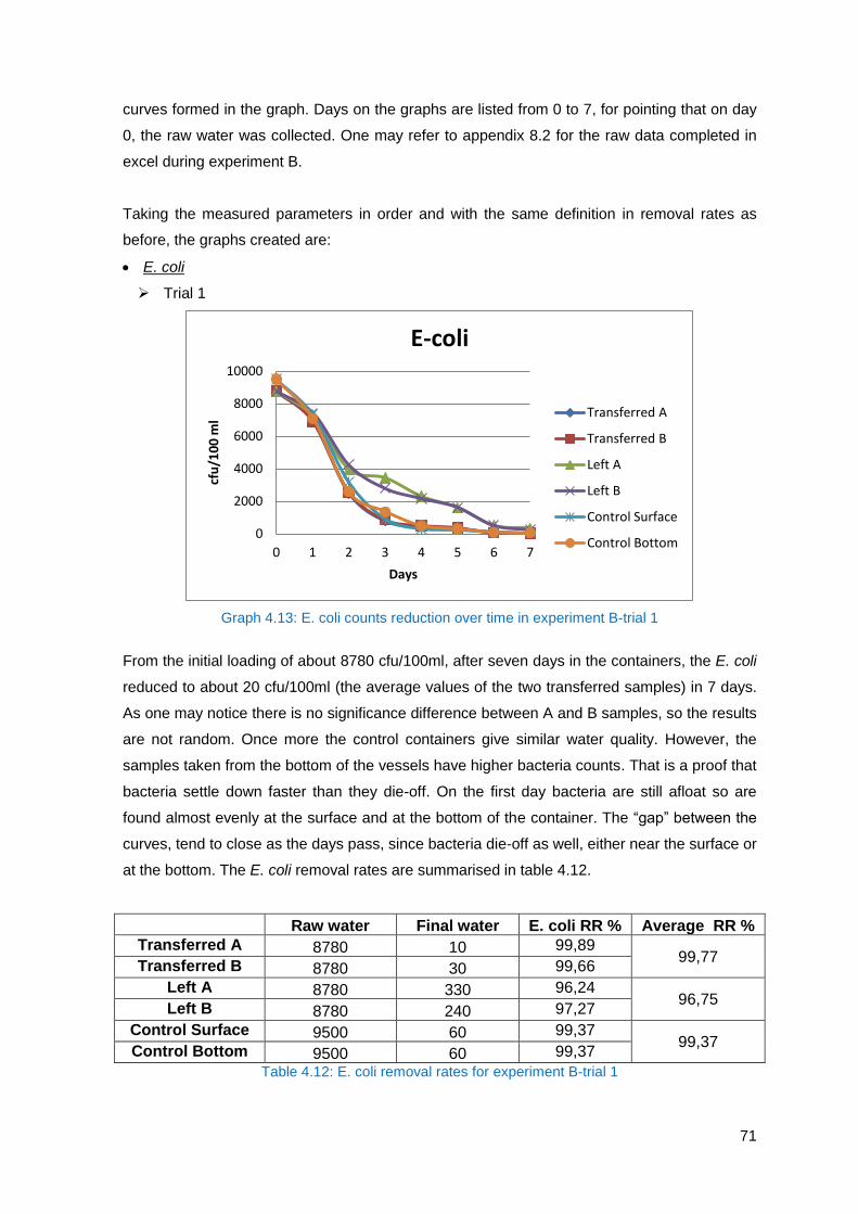
71

curves formed in the graph. Days on the graphs are listed from 0 to 7, for pointing that on day

0, the raw water was collected. One may refer to appendix 8.2 for the raw data completed in

excel during experiment B.

Taking the measured parameters in order and with the same definition in removal rates as

before, the graphs created are:

E. coli

Trial 1

Graph 4.13: E. coli counts reduction over time in experiment B-trial 1

From the initial loading of about 8780 cfu/100ml, after seven days in the containers, the E. coli

reduced to about 20 cfu/100ml (the average values of the two transferred samples) in 7 days.

As one may notice there is no significance difference between A and B samples, so the results

are not random. Once more the control containers give similar water quality. However, the

samples taken from the bottom of the vessels have higher bacteria counts. That is a proof that

bacteria settle down faster than they die-off. On the first day bacteria are still afloat so are

found almost evenly at the surface and at the bottom of the container. The “gap” between the

curves, tend to close as the days pass, since bacteria die-off as well, either near the surface or

at the bottom. The E. coli removal rates are summarised in table 4.12.


Transferred A 8780 10 99,89 99,77

Transferred B 8780 30 99,66

Left A 8780 330 96,24 96,75

Left B 8780 240 97,27

Control Surface 9500 60 99,37 99,37

Control Bottom 9500 60 99,37

Table 4.12: E. coli removal rates for experiment B-trial 1

0

2000

4000

6000

8000

10000

0 1 2 3 4 5 6 7

cfu

/10

0 m

l

Days

E-coli

Transferred A

Transferred B

Left A

Left B

Control Surface

Control Bottom

72

Trial 2

Graph 4.14: E. coli counts reduction over time in experiment B-trial 2

From the initial loading of about 17100 cfu/100ml, after seven days in the containers, the E.

coli reduced to about 125 cfu/100ml (the average values of the two transferred samples) in 7

days. Again, there is no significance difference between A and B samples, the control

containers give similar water quality and the samples taken from the bottom of the vessels

have higher bacteria counts. The E. coli removal rates are summarised in table 4.13.


Transferred A 17400 120 99,31 99,27

Transferred B 16800 130 99,23

Left A 17400 510 97,07 96,78

Left B 17400 610 96,49

Control Surface 16800 130 99,23 98,99

Control Bottom 16800 210 98,75

Table 4.13: E. coli removal rates for experiment B-trial 2

In trial 1 and 2, same water was used, so all the other parameters are stable, therefore it is

easier to comment on the bacteria removal rates for different bacteria loadings. The reduction

rate is similar, around 99%, in spite of the initial bacteria counts. Trial 2 final water though is

quite contaminated to be characterized of low risk. Yet the treatment is undeniable. Interesting

fact is that the bacteria counts seem to drop more rapidly, when the loading of bacteria is

bigger, especially in the first day of storage. Characteristically, for transferred water only,

looking at the reduction rates percentage, graph 4.15 shows the different “speed” at which

bacteria reduce. The average values of A and B where used for each trial in this graph.

0

2000

4000

6000

8000

10000

12000

14000

16000

18000

20000

0 1 2 3 4 5 6 7

cfu

/10

0 m

l

Days

E-coli

Transferred A

Transferred B

Left A

Left B

Control Surface

Control Bottom

73

Graph 4.15: E. coli reduction rates for transferred water in both trials in experiment B

Since the suspended solids are the same in both trials, this effect doesn’t have to do with the

attachment to any solids. One possible explanation is that the bigger population of bacteria,

assists flocculation, as explained in section 2.2.4, therefore the settlement is quicker. Another

possible explanation, that needs further research comes from the fact that trial 2 water is partly

loaded with laboratory cultivated E. coli. These may have a different behaviour compared to

naturally grown E. coli. Laboratory bacteria mixed in the raw water, seem to find themselves in

a new environment with natural characteristics. Being grown and kept in fridge conditions,

make them less adaptable to changes and robust. Therefore, natural water may come as a

shock and once they found themselves in it, they rapidly died off.

That fact could also explain why the speed of the reduction for the natural bacteria (trial 1) is

higher on day 2 than day 1. These bacteria may be suddenly restricted within a pot, but it

takes at least a day for the conditions like temperature, depletion of nutrients and so forth to

start happening in such an extent that bacteria will begin to be affected. Maybe in larger

containers these more adaptable bacteria, will need more days until they are affected by the

changes. One couldn’t trace literature to support this argument properly. The idea though was

based on plenty of articles found under the google search term “in vitro-in vivo E. coli” (in vitro:

in laboratory conditions, in vivo: in realistic conditions). They are usually examined from

medical researchers to conclude on the effectiveness of various pharmaceutical products and

not specifically on the in vivo-in vitro differences. The key idea though is that they may

respond in similar way, but they do respond with different rates. Characteristically, just in an

attempt to show how in vitro E. coli are less resilient, in a particular experiment by (Kolling et

al. 2001), it is stated that they did not recover in vitro, whereas there are studies that they

recover in vivo.

0,00

20,00

40,00

60,00

80,00

100,00

1 2 3 4 5 6 7

%

Days

E-coli

Transferred trial 1

Transferrred trial 2

74

For the rest parameters, the graphs shown here are from trial 1. This is done for space

economy and writing efficiency, since the initial water quality, apart from the bacteria loading,

is identical and the results between the trials didn't differ that much. The graphs for trial 2 are

placed in the appendices, without comments. Instead of placing all the graphs in this section,

summary tables for both trials are shown.

Temperature

Graph 4.16: Temperature over time in experiment B-trial 1

Ambient (air) temperature is shown in this graph, since this was the only factor altering the

water temperature. The containers are relatively small, thus temperature is stable through all

the water body. Temperature is overall stable, with table 4.14 summarizing the average

temperatures from all trials.

Average (oC)


Transferred 14,1 19,78

Left 14,1 19,78

Control Surface 14,1 19,20

Control Bottom 14,1 19,20 Table 4.14: Average temperature for all trials in experiment B

0

5

10

15

20

25

0 1 2 3 4 5 6 7

o C

Days

temperature

Transferred A

Transferred B

Left A

Left B

Control Surface

Control Bottom

Air

75

Colour

Graph 4.17: Colour reduction over time in experiment B-trial 1

Colour levels overall reduce, as suspended solids settle. The water left in the vessel contained

more suspended matter, therefore the colour levels were higher and the reduction rates lower.

It seems as if settlement occurred more significantly during the third day, if colour is connected

only to the suspended solids. This is false proof though. At that point the “left” volume was

altered from 1 litre to 0,5 litres. Therefore the water was more dense in suspended solids and

they were captured in larger quantities from the syringe. Also, note that the random effect in

experiment B was smaller, especially for the “left” water, which was less than 1 litre, since that

allowed a more “representative” fluid entering the syringe. Table 4.15 shows the average

colour reduction for all trials.

Colour (Hazen)

Trial Raw water Final water Colour RR % Average RR %

Transferred A

1 144 59 59,03

56,06 2 143 65 54,55

Transferred B

1 145 61 57,93

2 146 69 52,74

Left A

1 144 95 34,03

30,10 2 143 109 23,78

Left B

1 145 86 40,69

2 146 114 21,92

Control Surface

1 145 64 55,86

56,20 2 160 70 56,25

Control Bottom

1 145 65 55,17

2 160 68 57,50 Table 4.15: Average colour reduction for all trials in experiment B

0

20

40

60

80

100

120

140

160

0 1 2 3 4 5 6 7

Haz

en

Days

colour

Transferred A

Transferred B

Left A

Left B

Control Surface

Control Bottom

76

Turbidity

Graph 4.18: Turbidity reduction over time in experiment B-trial 1

Turbidity is inter-connected with the suspended solids, so it is logical for the turbidity levels to

drop, along with the settlement of the suspended solids. Again the “left” samples with the

higher content on suspended solids have higher turbidity levels and lower reduction rates. The

more significant settlement seemed to take place on day 3 again, but again this is due to the

change in the “left” volume, as explained before. The abnormal value of the “left B” curve in

day 1 is probably due to some sort of procedural or laboratory mistake, since it doesn’t seem

to appear elsewhere indirectly. The two trial results are summarised in table 4.16.

Turbidity (NTU)

Trial Raw water Final water Turbidity RR % Average RR %

Transferred A

1 12,1 2,24 81,49

75,26 2 12,4 3,11 74,92

Transferred B

1 12,1 3,10 74,38

2 11,8 3,51 70,25

Left A

1 12,1 5,65 53,31

51,13 2 12,4 6,18 50,16

Left B

1 12,1 5,50 54,55

2 11,8 6,31 46,53

Control Surface

1 11,7 2,98 74,53

73,04 2 12,7 3,25 74,41

Control Bottom

1 11,7 3,05 73,93

2 12,7 3,90 69,29 Table 4.16: Average turbidity reduction for all trials in experiment B

0

2

4

6

8

10

12

14

16

0 1 2 3 4 5 6 7

NTU

Days

turbidity

Transferred A

Transferred B

Left A

Left B

Control Surface

Control Bottom

77

pH

Graph 4.19: pH over time in experiment B-trial 1

pH in all trials slightly rises, around 1 pH degree. That could re-affirm the previously stated

theory that (H+) ions attach with the negatively charged E. coli and that can result in a rise of

pH. In this experiment where the loading is higher, pH rises more than in experiment A. In

table 4.17, the pH rise for all trials is shown.

pH

Trial Raw water Final water pH rise % Average rise %

Transferred A

1 7,0 8,0 14,29

13,74 2 7,1 8,1 14,08

Transferred B

1 7,1 8,1 14,08

2 7,2 8,1 12,50

Left A

1 7,0 8,0 14,29

13,74 2 7,1 8,1 14,08

Left B

1 7,1 8,1 14,08

2 7,2 8,1 12,50

Control Surface

1 7,2 8,1 12,50

10,70 2 7,3 8,0 9,59

Control Bottom

1 7,2 8,0 11,11

2 7,3 8,0 9,59 Table 4.17: Average pH rise for all trials in experiment B

7,0

7,2

7,4

7,6

7,8

8,0

8,2

0 1 2 3 4 5 6 7

Days

pH

Transferred A

Transferred B

Left A

Left B

Control Surface

Control Bottom

78

Total Dissolved Solids

Graph 4.20: Total Dissolved Solids over time in experiment B-trial 1

Total dissolved solids drop from 270 ppm to 260 ppm and seem to remain stable through the

days. As explained before, TDS should not be related only to sedimentation of suspended

solids. If that was the case, the curve would follow the suspended solids one. Minerals, salts,

anions and so forth, may be released or trapped through various procedures, therefore it is

difficult to explain the TDS curves. Table 4.18 shows the average TDS results from all trials.

TDS (ppm)

Raw water Final water TDS RR%

Transferred 270 260 3,7

Left 270 260 3,7

Control 270 260 3,7

Table 4.18: Average TDS values for all trials in experiment B

Dissolved Oxygen

Graph 4.21: Dissolved oxygen over time in experiment B-trial 1

258

260

262

264

266

268

270

272

0 1 2 3 4 5 6 7

pp

m

Days

TDS

Transferred A

Transferred B

Left A

Left B

Control Surface

Control Bottom

8

8,2

8,4

8,6

8,8

9

9,2

9,4

9,6

0 1 2 3 4 5 6 7

mg/

l

Days

dissolved oxygen

Transferred A

Transferred B

Left A

Left B

Control Surface

79

Note that in this graph “control bottom” is missing, since the DO meter probe wasn’t long

enough to reach the bottom of the stationary water. Initially, DO was around 9,5 mg/l. As the

first days passed, the DO levels dropped for the same reasons explained in experiment A.

However, in experiment B, levels seemed to rise again after the third day. Transferred water

became less in volume, since every day the settled water was thrown away. Therefore the

column of water became smaller and it was easier for the remaining water layers to intermix

after every pouring procedure. That assisted oxygen exchange with atmosphere. The smaller

volume of the “left” water after day 3, allowed more oxygen to pass into the fluid as well, thus

there was a rise in DO levels as well. Temperature rising and bacteria feeding, which resulted

in oxygen reduction, may be applicable in this case as well, but they were not as strong as the

aeration mechanism. Table 4.19 shows the DO reduction in all trials. Indeed, stationary

“control” water with no aeration chances, dropped the DO levels most of all.

DO (mg/l)

Trial Raw water Final water DO RR % Average RR %

Transferred A

1 9,5 8,9 6,32

6,05 2 9,5 9,0 5,26

Transferred B

1 9,5 9,0 5,26

2 9,5 8,8 7,37

Left A

1 9,5 9,0 5,26

5,53 2 9,5 8,9 6,32

Left B

1 9,5 9,0 5,26

2 9,5 9,0 5,26

Control Surface

1 9,4 8,5 9,57 9,04

2 9,4 8,6 8,51

Table 4.19: Average DO reduction for all trials in experiment B

Suspended Solids

Graph 4.22: Suspended Solids over time in experiment B-trial 1

0

2

4

6

8

10

12

14

16

18

0 1 2 3 4 5 6 7

mg/

l

Days

suspended solids

Transferred A

Transferred B

Left A

Left B

Control Surface

Control Bottom

80

Suspended solids measurements and therefore the graphs again are not very uniform. The

laboratory mistake of using unwashed filters for the SS measurement was not repeated this

time. Day 3, where the SS level in “left” water became more dense can be seen. For the rest

of the measurements, there is no clear explanation why they fluctuate. The author may think

that since these figures are very small when measured in g/100 ml in the laboratory scale,

0,0001 g/100 ml will result in 1 mg/l in the graph. It is very easy to have 0,0001 g/100 ml

fluctuation in the scale and on the SS, but on the graph this is reproduced with larger

significance than it actually is. Overall though this time, the curves drop, since solids settle

down. Table 4.20 summarises the reduction of the SS from both trials.

SS (mg/l)

Trial Raw water Final water SS RR % Average RR %

Transferred A 1 16 1 93,75

90,08 2 17 2 88,24

Transferred B 1 12 1 91,67

2 15 2 86,67

Left A 1 16 8 50,00

48,43 2 17 9 47,06

Left B 1 12 6 50,00

2 15 8 46,67

Control Surface 1 14 1 92,86

88,10 2 15 1 93,33

Control Bottom 1 14 1 92,86

2 15 4 73,33 Table 4.20: Average SS reduction for all trials in experiment B

As expected, transferred water has less SS as days passed, therefore higher reduction rates,

compared to the “left” water, which gathered all the settled matter. Control water from the

surface logically shows relatively high RR, since SS settled and moved away from the top.

Note though that the RR of the bottom is false. By taking samples always from the centre of

the container, SS were gradually removed from this area (see section 4.2.4). Therefore, SS

seem falsely to reduce.

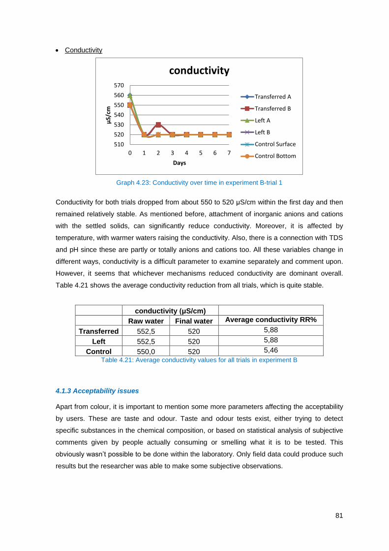
81

Conductivity

Graph 4.23: Conductivity over time in experiment B-trial 1

Conductivity for both trials dropped from about 550 to 520 μS/cm within the first day and then

remained relatively stable. As mentioned before, attachment of inorganic anions and cations

with the settled solids, can significantly reduce conductivity. Moreover, it is affected by

temperature, with warmer waters raising the conductivity. Also, there is a connection with TDS

and pH since these are partly or totally anions and cations too. All these variables change in

different ways, conductivity is a difficult parameter to examine separately and comment upon.

However, it seems that whichever mechanisms reduced conductivity are dominant overall.

Table 4.21 shows the average conductivity reduction from all trials, which is quite stable.

conductivity (μS/cm)

Raw water Final water Average conductivity RR%

Transferred 552,5 520 5,88

Left 552,5 520 5,88

Control 550,0 520 5,46

Table 4.21: Average conductivity values for all trials in experiment B

4.1.3 Acceptability issues

Apart from colour, it is important to mention some more parameters affecting the acceptability

by users. These are taste and odour. Taste and odour tests exist, either trying to detect

specific substances in the chemical composition, or based on statistical analysis of subjective

comments given by people actually consuming or smelling what it is to be tested. This

obviously wasn’t possible to be done within the laboratory. Only field data could produce such

results but the researcher was able to make some subjective observations.

510

520

530

540

550

560

570

0 1 2 3 4 5 6 7

μS/

cm

Days

conductivity

Transferred A

Transferred B

Left A

Left B

Control Surface

Control Bottom

82

Applying to both experiments, one perceived the raw water to have a strong “damp” odour, like

wet soil, which was expected since the water was collected from the stream. When water was

decanted, by either siphoning or pouring, either for 3 or 7 days, this odour level dropped every

day. It never disappeared completely, but it wasn’t discouraging any more. After the first two

days, the reduction rate of this annoying odour, was thought to drop as well. Interestingly, in

the control buckets, where water was stable, the odour remained almost as strong as it was

initially. This supported the fact that aeration improves the water quality further and is an

active mechanism in the three-pot system. Last point to mention, is that the exact moment the

lid was taken off, the smell was a lot stronger. In that sense, the researcher thought that while

the lid is necessary to prevent recontamination, it may be inhibiting the odour reduction. Of

course, contamination of water is more important than the acceptability issue of odour, thus

the lid is advised in any case.

The overall appearance of the pots as noticed through the experiments should be mentioned

as well, when it comes to acceptability. Physical substances found in surface water, apart from

suspended solids, were various organic matter like leaves and small pieces of wood, various

small organisms, like dead-alive bugs and oils. Depending on their density, some sunk in the

bottom and others remained floating at the surface. Before decanting the water, the floating

substances were carefully removed. That can be performed by the user easily, so as to have

more acceptable water finally. These observations generated the idea that floatation should be

included in the purification mechanism as well.

Figure 4.2: Small leaves (a) and a dead bug (b) floating on the surface (author 2012)

Moreover, according to the author’s perception, algae growth was noticed to a very small

extent. This green substance didn't appear at the whole container with such sort retention

times, but had the form of an algal ring at the border where the water met the edge of the

a

b

83

bucket. The formation of this ring kept reducing every day the water was decanted. On the

control containers, the thickness of this ring was bigger, since water remained stagnant. Pots

need periodical cleaning from algae as well, if they are to be used continuously for the three-

pot system. Note, that no tests were carried out to confirm if that was algae indeed.

Figure 4.3: Algal ring near the surface (author 2012)

Last issue traced was the flotation of oils on the surface to a very small extent. Unfortunately,

that couldn’t be captured by the camera. It looked like a thin film with different sized circles

which reflected the laboratory lights a bit differently than plain water, thus they were spotted.

Initially, one thought that this were some sort of oils or even worse, this could be the initial

stage of a biofilm formation (i.e. surface attached matrix composed of micro-organisms),

concerned about E. coli floating instead of settling. (For details on biofilm formation, one may

refer to the particular chapter in (Mara et al. 2003) on p. 337). Fortunately, this wasn’t the case

of a biofilm. It was observed, that this film wasn’t present any more on day 2 when water was

siphoned, but only when it was poured. If it was a biofilm formed from floating bacteria, it

would most likely be re-formed in the next pot as well. However, the particular “film” seemed to

be transferred rather than formed. When pouring, water falls from the surface into the next pot,

so the “film” was carried along. When siphoning, water was sucked from the level where the

siphon was placed and the procedure was stopped before surface water reached that level, so

as not to suck air in. As a result, the “film” remained at the previous pot and thrown away with

the rest of the bottom sediments. In that sense, this was most likely a film made out of oils

present in the water that floated at the surface. That belief was confirmed after experiment B.

In this case, the water that was collected from the stream was after having rained. The stream

flow has increased and therefore the oils were diluted. With smaller oil content, the film wasn’t

formed this time. If it was a matter of biofilm, the bigger bacteria loading in experiment B,

should have produced a thicker biofilm layer.

4.2 Discussion and Analysis

In this section, the five objectives will be answered in particular and that will lead to the

discussion of the overall aim of the project.

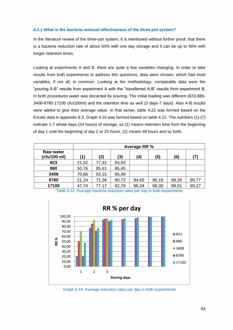
84

4.2.1 What is the bacteria removal effectiveness of the three-pot system?

In the literature review of the three-pot system, it is mentioned without further proof, that there

is a bacteria reduction rate of about 50% with one day storage and it can be up to 90% with

longer retention times.

Looking at experiments A and B, there are quite a few variables changing. In order to take

results from both experiments to address this questions, data were chosen, which had most

variables, if not all, in common. Looking at the methodology, comparable data were the

“pouring A-B” results from experiment A with the “transferred A-B” results from experiment B.

In both procedures water was decanted by pouring. The initial loading was different (823-880-

3408-8780-17100 cfu/100ml) and the retention time as well (3 days-7 days). Also A-B results

were added to give their average value. In that sense, table 4.22 was formed based on the

Excels data in appendix 8.3. Graph 4.24 was formed based on table 4.22. The numbers (1)-(7)

indicate 1-7 whole days (24 hours) of storage, so (1) means retention time from the beginning

of day 1 until the beginning of day 2 or 24 hours, (2) means 48 hours and so forth.

Average RR %

Raw water (cfu/100 ml) (1) (2) (3) (4) (5) (6) (7)

823 21,02 77,32 93,93

880 50,76 85,61 95,45

3408 70,86 93,15 95,99

8780 21,24 71,36 90,72 94,65 96,18 99,26 99,77

17100 47,74 77,17 92,79 96,34 98,39 98,91 99,27 Table 4.22: Average bacteria reduction rates per day in both experiments

Graph 4.24: Average reduction rates per day in both experiments

0,00

10,00

20,00

30,00

40,00

50,00

60,00

70,00

80,00

90,00

100,00

1 2 3

RR

%

Storing days

RR % per day

823

880

3408

8780

17100

85

The 50% reduction rate with one day of storage is reached by the 880 and 3408 cfu/100ml

samples, nearly reached by the 17100 cfu/100ml sample and is far from being reached by the

823 and 8780 cfu/100ml samples. It is difficult to comment with certainty on the results

because of the large number of variables affecting the purification mechanisms. As mentioned

within the literature review, it is difficult to predict every time the removal effectiveness based

on theoretical models. Bacteria basically are reduced due to sedimentation and natural die-off.

The variables on sedimentation mechanisms are: particle size and shape, particle density,

particle surface charge, liquid density, liquid viscosity, liquid temperature, salt content, settling

velocity, particles population, colloids and turbulence. Retention time and type of pathogen,

affect the natural die-off rates, along with the environmental conditions. Which is the dominant

variable or the particular inter-connections among them cannot be stated with certainty, as

these are alive organisms and any relationships are changing dynamically. An attempt to

conclude on some of these variables will be done, by keeping the rest constant to some extent.

The initial (raw) water quality characteristics in average are summarised in table 4.23, so that

comparisons can be made, assuming of course that there are no laboratory and calculation

mistakes.

823 880 3408 8780 17100

SS (mg/l) 5 3,5 13 14 16

Temperature (oC) 16,7 17,5 17 14,1 14,1

DO (mg/l) 8,4 8,5 8 9,5 9,5

pH 7,5 7,35 7 7,05 7,15

Conductivity (μS/cm) 710 660 673 555 550

TDS (ppm) 330 330 330 270 270

Colour (Hazen) 30 45 83 144,5 144,5

Table 4.23: Average water quality characteristics per sample in both experiments

Looking at the samples from experiment A and at two samples that reached the 50% limit

(880-3408 cfu/100ml) in particular, their variables are quite similar, except for the suspended

solids, where the difference is more significant. The bigger population of E. coli and of

suspended solids could explain why the reduction rate is bigger in the “3408” sample.

However, looking at the “823” and “880” samples, the bacteria loading and the suspended

solids are almost similar, as are all the other parameters too. There is no obvious explanation

why these two systems respond differently within the first day. One assumes that what is

characterized “small” difference for the laboratory calculations and the researcher’s eyes, can

play a significant role at a bacteria microscopic level, thus is very difficult to be captured. On

the other hand, since water was collected on different days, the E. coli themselves are not the

same. It may be just a case of finding the bacteria in a different stage of their growth cycle

86

(figure 2.6). The environmental conditions (oxygen, pH, temperature, nutrients, toxicity) just

prolong or speed up their natural death.

Similarly, looking at the experiment B samples (8780-17100 cfu/100 ml), where water was

collected in the same day and all the parameters are almost identical, the “17100” sample

almost reached the 50% limit, while the other one only reached 20%. The bigger population of

bacteria, actually assisting sedimentation, is one obvious explanation. However, it is very

important that half of this population is artificially added with laboratory cultivated E. coli. As

explained earlier, these bacteria may be less resilient, therefore dying faster than the natural

ones.

Lastly, looking at experiments A and B together, the samples with naturally found bacteria are

the “3408” and “8780” ones. In this case, bacteria loading doesn't seem to have the dominant

role, since the “3408” sample performs better. Nor do the suspended solids which are almost

similar. However, temperature is higher in the first sample, which can alter the water density or

raise the thermal energy, which in turn will increase the collisions between particles (Brown’s

law). Both phenomena assist flocculation and sedimentation. Moreover, oxygen is less in the

first sample, therefore bacteria, as all aerobic organisms, will survive less without it. Also, TDS

and conductivity figures are evidence of more anions, cations, salts and so forth. These

charged molecules can attach with E. coli probably more easily and assist flocculation.

In an attempt to triangulate the one-day retention time on bacterial efficiency, it is worth

mentioning the results found in (Singer, 2010, p. 73, table 4.11), even if that wasn’t the focus

of the particular research. Again the reduction rates of E. coli for 24 hours vary from 20,30%

up to 87,43% for different initial loadings, without necessarily the lower rates found in the less

contaminated water.

All these observations apply only on the first day samples. It is obvious from the graph that by

storing day (2), after 48 hours, even if all the variables are still different from one experiment to

the other, all the reduction rates are higher than 70% and by day 3, higher than 90%. For the

remaining days, the reduction rates rise slightly per day, reaching closer to 100%

effectiveness. The “speed” of the reduction rate drops significantly after passing day (2) and

keeps on reducing every extra day more. So the treatment process slows down after day (2).

Within each container, the conditions tend to be stabilized only after 24 hours of retention.

That seems to be the time needed by the bacteria on a 10 litre vessel to realize their limited

situation, thus start responding to that by dying-off (see figure 2.6) more quickly. Moreover,

after one day of stagnant water, sedimentation processes have occurred more significantly,

87

therefore the reduction rates are increased. Whichever of the two mechanisms is dominant in

the purification process, they both occur more significantly between 24 hours of retention (day

1) and 48 hours of retention (day(2)), thus the reduction rates are higher within that period.

Conclusion:

On the question of removal effectiveness, one day of storage doesn't necessarily lead to 50%

reduction of the bacteria, as claimed. It can be higher or lower. For longer retention times, this

figure is improved and it can exceed the claimed figure of 90%. The 90% figure is usually

reached within three storing days, no matter the initial contamination. It is undoubted more

effective to store the water longer than one day, but if this is the only drinking water available,

questions on the efficiency of storing the water longer arise.

4.2.2 How many days should the retention time be?

In the literature it is claimed that the retention time can be from 24 hours, up to 6 days. This

clearly leads back to question 4.2.1, but it was decided to be addressed separately, as it is

found in publications without reference to the reduction rates.

One day retention time reduces the bacteria loading, but as shown earlier, this reduction may

be quite low, not even close to 50% in some samples. The first day is the time needed for the

conditions in the water to be uniform, therefore the bacteria start dying more significantly after

that. One day of storage wouldn't be advised in order to be more certain that sufficient

treatment has taken place. After two days of storage, the reduction rate has increased

significantly in all samples. If the need to use the water is immediate and another day cannot

be spared for treatment, two days of storage is advised, since it seems to be the minimum

retention time with the highest possible results for all samples. After 48 hours, any more

time/days are beneficial for the bacteria removal. Either this is 6 days as mentioned, either 7

as tested, either more, even if sedimentation ceases at some point, bacteria naturally keep on

dying-off. Therefore, the longer the better as claimed in the literature. The reduction numbers

for three days exceed 90% and after that period, reduction tends to reach 100%.

Note that in general, the“100%” figure needs attention. Percentages in the reduction rates are

disconnected from the actual bacteria loading on the initial or final water. Therefore they can

be misleading. 100% removal rate doesn't mean zero pathogens in the water. ln addition, 100%

rate is often 99,5% rate, rounded up. As one can see characteristically in tables 4.13, for

transferred water the average removal rate is 99,27%, while the bacteria are still 125

cfu/100ml, far from being zero.

88

Conclusion:

On the question of retention time days, treatment takes place every storage day, but the

longer the storage period the better. One day is the minimum. Two days are advised since this

is the minimum retention time with the maximum results, if one compares all the samples.

Three days are optimum, since the reduction rates reach the level of 90% reduction. More

days lead to further improvement. It is undoubted more effective to store the water longer than

one day, but again if this is the only drinking water available, questions on the efficiency of

storing the water longer rise. Acceptable levels of E. coli concentrations are commented in

section 4.3.

4.2.3 Is siphoning more effective than pouring?

Within the literature it is claimed without further referencing that it is better to decant the water

from one pot to the other by siphoning rather than pouring, because the sediments will be less

disturbed. In experiment A siphoning and pouring was tested to see whether this is true. Table

4.24 summarises the average reduction rates for each bacteria loading, taken from appendix

8.3. Graph 4.25 is based on table 4.24, focusing on the difference between the rates.

Average RR %

Raw water (cfu/100 ml)

Method 1 2 3

823 Siphon 29,93 85,01 95,95

Pour 21,02 77,32 93,93

880 Siphon 64,02 87,88 95,83

Pour 50,76 85,61 95,45

3408 Siphon 69,10 92,76 96,58

Pour 70,86 93,15 95,99

Table 4.24: Average reduction rate % for bacteria loading per method in experiment A

21,02

77,32 93,93

8,91

7,70 2,02

1 2 3

823

Pouring Siphoning

50,76

85,61 95,45 13,26

2,27 0,38

1 2 3

880

Pouring Siphoning

89

Graph 4.25: Difference in the E. coli reduction rates between siphoning and pouring per day and per sample in experiment A

In the first two samples, siphoning is more effective than pouring in the bacteria removal, while

in the third sample things are opposite. The differences are not major and they tend to get

smaller with more days of retention or as pointed in question 4.2.2, the longer retention time

the better. Assuming that the figures are correct, the presence of the third sample, doesn’t

allow clear conclusion on the bacteria removal. In an attempt to rationalise this fact, one would

think that it has to do with the higher bacteria loading and the suspended solids content as

well, (the “3408” sample has double suspended solids compared to the other two). Both

loadings, assist flocculation, thus sedimentation. If that is the case, in the first two samples,

sedimentation takes place more slowly, so the bacteria are afloat for longer time within the

water body. In that sense, when pouring is practiced in the first two samples, bacteria which

are dispersed in the main water body, flow to the next pot. When siphoning is practiced, water

is taken from the point where the siphon is placed and this is near the bottom (careful not in

touch with the bottom, a few cm above). So in the first two samples, where sedimentation

hasn't occurred in a great extent, the water near the bottom may be of better quality. On the

contrary, on the “3408” sample, where sedimentation is faster, pouring water from the surface

is of better quality, while siphoning water from the bottom is more contaminated. To sum up,

the treatment is basically a matter of how much settlement has occurred in a sense and not of

the disturbance caused to the suspended solids as stated in the literature. Besides, pouring

was done in a gentle way as well, making sure that the sediments were not disturbed, so less

likely to be carried over in the next pot.

Apart from the bacteria effectiveness, looking at the rest water quality parameters of the final

water in section 4.1.1 and using the average figures for all three samples, table 4.25 was

made.

70,86 93,15 95,99

-1,76 -0,39

0,59

1 2 3

3408

Pouring Siphoning

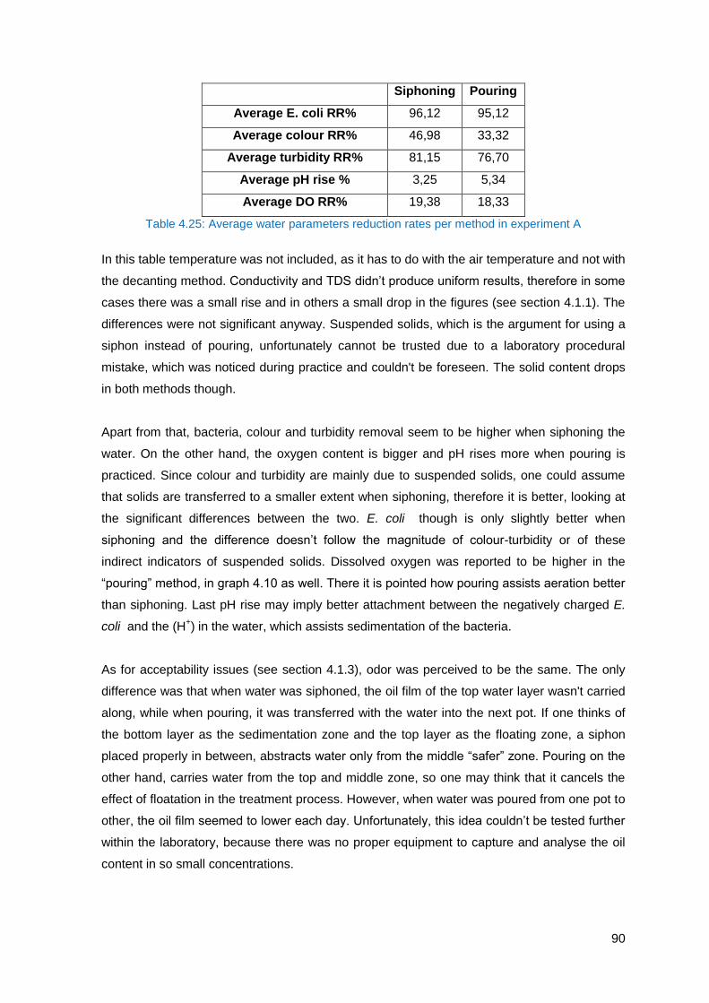
90

Siphoning Pouring

Average E. coli RR% 96,12 95,12

Average colour RR% 46,98 33,32

Average turbidity RR% 81,15 76,70

Average pH rise % 3,25 5,34

Average DO RR% 19,38 18,33

Table 4.25: Average water parameters reduction rates per method in experiment A

In this table temperature was not included, as it has to do with the air temperature and not with

the decanting method. Conductivity and TDS didn’t produce uniform results, therefore in some

cases there was a small rise and in others a small drop in the figures (see section 4.1.1). The

differences were not significant anyway. Suspended solids, which is the argument for using a

siphon instead of pouring, unfortunately cannot be trusted due to a laboratory procedural

mistake, which was noticed during practice and couldn't be foreseen. The solid content drops

in both methods though.

Apart from that, bacteria, colour and turbidity removal seem to be higher when siphoning the

water. On the other hand, the oxygen content is bigger and pH rises more when pouring is

practiced. Since colour and turbidity are mainly due to suspended solids, one could assume

that solids are transferred to a smaller extent when siphoning, therefore it is better, looking at

the significant differences between the two. E. coli though is only slightly better when

siphoning and the difference doesn’t follow the magnitude of colour-turbidity or of these

indirect indicators of suspended solids. Dissolved oxygen was reported to be higher in the

“pouring” method, in graph 4.10 as well. There it is pointed how pouring assists aeration better

than siphoning. Last pH rise may imply better attachment between the negatively charged E.

coli and the (H+) in the water, which assists sedimentation of the bacteria.

As for acceptability issues (see section 4.1.3), odor was perceived to be the same. The only

difference was that when water was siphoned, the oil film of the top water layer wasn't carried

along, while when pouring, it was transferred with the water into the next pot. If one thinks of

the bottom layer as the sedimentation zone and the top layer as the floating zone, a siphon

placed properly in between, abstracts water only from the middle “safer” zone. Pouring on the

other hand, carries water from the top and middle zone, so one may think that it cancels the

effect of floatation in the treatment process. However, when water was poured from one pot to

other, the oil film seemed to lower each day. Unfortunately, this idea couldn’t be tested further

within the laboratory, because there was no proper equipment to capture and analyse the oil

content in so small concentrations.

91

As it is made obvious, siphoning can perform better with some variables, but pouring does so

with some others. Since the purification mechanism of the three-pot system depends on many

variables, it is difficult to conclude on which variable is most important, therefore decide on

siphoning versus pouring. Besides, as already shown, each case is unique and theoretical

models are difficult to be predicted covering each possibility. To one’s personal opinion, both

methods are similarly effective, especially to bacteria reduction, which is the primary concern.

The rest parameters have more to do with aesthetic reasons and user acceptance. It is

understood once more that “similar” reduction rates may not always refer to similar final water

quality characteristics, as pointed in question 4.2.2. However, in this case the final bacterial

loading is similar in each case along with the reduction rate, as shown in tables 4.3-4.4-4.5.

Thus one can refer to these two methods having similar reduction effectiveness. The reduction

effectiveness is becoming more identical when more retention days are given to the water, as

explained in question 4.2.2

Conclusion:

On the question of whether is siphoning more effective than pouring, one would suggest that

for bacteria reduction they are practically the same, especially after 48 hours of storage. For

the aeration treatment process, pouring is slightly more effective and for turbidity reduction

siphoning is better.

Since the purification mechanism of the three-pot system depends on many variables, it is

difficult to conclude on which variable is most important, therefore decide on siphoning versus

pouring. Personally, one concludes that both methods treat water significantly, so it is

pointless dilemma the “siphoning versus pouring”. It is similar to asking HWTS or centralized

treatment method, as previously discussed. Since both improve water, they should both be

adopted in the appropriate situation.

“Appropriate” raises some issues of efficiency worth to mention. Pouring is a simple procedure,

easily performed by anyone, fast (10 litres were poured in about 25 sec), with no additional

material needed. Siphoning requires some basic co-ordination skills, it is a slow procedure (10

litres were poured in about 3,5 min) and a siphon needs to be available or a flexible tube. A

flexible tube, like a straw can be used to siphon the water out, initializing it by sucking the first

water by mouth. Any siphon needs regular cleaning as well and careful handling to prevent

recontamination of water. Sucking the water by mouth, may pose health risks to the person

practicing it, if by accident swallows the contaminated water. On the other hand, if the

containers are of great volume, lifting and pouring may be impossible and in this case,

siphoning is needed or at least two people lifting the containers. Moreover, pouring needs to

be done carefully, without much disturbance which can re-suspend the solids near the bottom

92

and any bacteria trapped in them. So, one point of view can be to use a siphon to prevent

indirectly the user from practicing wrong the “pouring” method.

4.2.4 Is the surface water of better quality than the water at the bottom?

Within the literature it is claimed that water near the surface of the pot is of better quality than

that of the bottom. In experiment B, measurements to test surface and bottom quality were

done directly in the stable (control) buckets and indirectly in the other pots, by sampling the

water left on the previous pot and the water transferred on the next pot.

Looking at the E. coli counts and their reduction rates% in appendix 8.3.4 and 8.3.5 for the

control surface and control bottom rows, will notice that they are similar for all days or in some

cases the “bottom” sample has higher rates from the “surface” one. Since the indirect

measurements did not agree not this fact appeared logical, it was concluded that these figures

do not represent the real situation, therefore they are not worth presenting in this section. The

cause for this false result was figured out. To sample the water from the control pot without

disturbance a syringe was used. The syringe was always placed in the centre of the circular

bottom of the pot, to assist procedural repetition. However, this proved to be faulty, because

the syringe was gradually clearing the particular spot each day by sucking 100 ml out. This

was noticed from the suspended solids which “disappeared” from the centre of the pot as well.

Therefore, these results will not be used.

Figure 4.4: Syringe clearing out the centre of the pot (author 2012)

Looking at the E. coli counts in appendix 8.3.4 and 8.3.5 for the transferred and left water rows,

the surface water is of better quality in both trials. Since the average reduction rates didn’t

differ significantly between the trials, the mean values from trial 1 and 2 will be used to

address this question. Thus table 4.26 was formed. Graph 4.26, based on table 4.26, focuses

on the difference between the rates.

93

Transferred Left

Average RR% 1 34,49 17,25

Average RR% 2 74,26 37,13

Average RR% 3 91,76 45,88

Average RR% 4 95,50 47,75

Average RR% 5 97,29 48,64

Average RR% 6 99,09 49,54

Average RR% 7 99,52 49,76 Table 4.26: Average E. coli reduction rates per method in experiment B

Graph 4.26: Difference in the E. coli reduction rates between bottom and surface water per day in experiment B

It is obvious from the appendix that transferred or surface water has lower bacteria counts and

the reduction rates are higher as well, compared with the bottom water. This verifies that

sedimentation is part of the purification process of the three-pot system. Since bacteria tend to

settle at the bottom, they exist in greater counts there. The difference in quality between them

gets smaller as more days are given for retention. Since bacteria die-off, either found at the

bottom or the surface, even if sedimentation ceases at some point, more retention days could

theoretically lead to the same water quality at the surface and at the bottom. Moreover, in

(Nath et al. 2006, p. 39) it is stated for another treatment method, that pathogens usually

remain viable in the bottom and need to be separated from the upper cleaner water body.

As for the rest quality characteristics presented in section 4.1.2, most of them don’t show

significant differences, apart from the suspended solids. These are in higher concentrations at

the bottom where they have settled. That leads to bottom water having higher turbidity and

colour levels as well, compared to the surface. These average reduction rates for the final

water, from both samples, summarised from section 4.1.2, form table 4.27.

30,43

52,13 63,75

76,79 87,95 95,08 96,74

4,06

22,13

28,01 18,70

9,34 4,01 2,78

1 2 3 4 5 6 7

Left Transferred

94

Transferred Left

Average E. coli RR% 99,52 96,77

Average colour RR% 56,06 30,10

Average turbidity RR% 75,26 51,13

Average ss RR % 90,08 48,43

Table 4.27: Average water parameters reduction rates for surface and bottom water

When it comes to acceptability issues (see section 4.1.3), odor was perceived to be the same.

Moreover, surface water retains the floating substances, while bottom water the settled ones.

The floating matter though were less than the settled in this case and could be manually

removed, thus transferred water was cleaner than the “left” one. Since bacteria tend to settle

and not to float, bottom water could be more dangerous than surface water in any case,

regardless of the appearance.

Conclusion:

To the question of which point has higher quality within the vessel, surface water is indeed

better than the bottom one. Their difference gets smaller with more retention days. However,

in order to be on the safe side, it is recommended always to abstract water from the near the

surface. When sedimentation is part of the treatment method, it is not advised to use

containers with a tap placed near the bottom, from where users will abstract water to drink. In

that sense it is wiser for the user to pour the drinkable water from the surface when he wants

to drink or to use an appropriately clean cup to collect water from near the surface.

4.2.5 How many pots should be used?

In the literature it is stated without further referencing that three-pots are advised, two-pots are

considered as minimum, but even with one pot the treatment may work.

This is translated in days of retention basically. It is a way to make sure that the user will allow

sufficient time for the treatment to take place before consuming the water. By suggesting three

pots, one for each day, water settles for 72 hours before consumption, while two pots allow 48

hours for retention. Without giving further explanation or training to the user, by suggesting

three or two pots safeguards indirectly, that significant treatment will have taken place. In that

sense, one pot is not advised. However, it is stated that if no other pots are available, it can be

used, but more days should be given for retention. One pot shouldn’t mean one day of storage.

Even if treatment has occurred after 24 hours, it is always safer to allow more days for that

(see questions 4.2.1 and 4.2.2 for details).

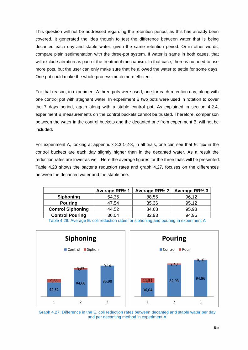
95

This question will not be addressed regarding the retention period, as this has already been

covered. It generated the idea though to test the difference between water that is being

decanted each day and stable water, given the same retention period. Or in other words,

compare plain sedimentation with the three-pot system. If water is same in both cases, that

will exclude aeration as part of the treatment mechanism. In that case, there is no need to use

more pots, but the user can only make sure that he allowed the water to settle for some days.

One pot could make the whole process much more efficient.

For that reason, in experiment A three pots were used, one for each retention day, along with

one control pot with stagnant water. In experiment B two pots were used in rotation to cover

the 7 days period, again along with a stable control pot. As explained in section 4.2.4,

experiment B measurements on the control buckets cannot be trusted. Therefore, comparison

between the water in the control buckets and the decanted one from experiment B, will not be

included.

For experiment A, looking at appenndix 8.3.1-2-3, in all trials, one can see that E. coli in the

control buckets are each day slightly higher than in the decanted water. As a result the

reduction rates are lower as well. Here the average figures for the three trials will be presented.

Table 4.28 shows the bacteria reduction rates and graph 4.27, focuses on the differences

between the decanted water and the stable one.

Average RR% 1 Average RR% 2 Average RR% 3

Siphoning 54,35 88,55 96,12

Pouring 47,54 85,36 95,12

Control Siphoning 44,52 84,68 95,98

Control Pouring 36,04 82,93 94,96 Table 4.28: Average E. coli reduction rates for siphoning and pouring in experiment A

Graph 4.27: Difference in the E. coli reduction rates between decanted and stable water per day and per decanting method in experiment A

44,52

84,68 95,98 9,83

3,87 0,14

1 2 3

Siphoning

Control Siphon

36,04

82,93 94,96

11,51

2,43 0,16

1 2 3

Pouring

Control Pour

96

It is obvious that stable water has lower reduction rates compared to the decanted one, either

water is siphoned or poured in the next pot. It can therefore be concluded that aeration assist

the treatment and is indeed part of the purification mechanism. On the other hand, bacteria

counts in the appendices, tend to equalize as more days pass. Or as depicted here, the gap

between the reduction rates once more tends to close. By day 3, the bacteriological quality in

the control bucket, is very close to the decanted water.

As for the rest water quality parameters, referring to the final water in section 4.1.1 and using

the average figures for all three samples, table 4.25 was made.

Siphoning Pouring Control Siphoning Control Pouring

Average E. coli RR% 96,12 95,12 95,98 94,96

Average colour RR% 46,98 33,32 37,89 40,61

Average turbidity RR% 81,15 76,70 82,19 83,37

Average pH rise % 3,25 5,34 6,25 6,25

Average DO RR% 19,38 18,33 26,67 20,88

Table 4.29: Average water parameters reduction rates per method in experiment A

Once more, temperature was not included, as it has to do with the air temperature and not

with the decanting method. Conductivity and TDS didn’t produce uniform results, therefore in

some cases there was a small rise and in others a small drop in the figures (see section 4.1.1).

The differences were not significant anyway. Suspended solids, unfortunately cannot be

trusted due to a laboratory procedural mistake, which was noticed during practice and couldn't

be foreseen. The solid content drops in any case though.

In the siphoning option, the stable bucket reduces colour less, reduces turbidity more, rises pH

more, and reduces oxygen more than in the siphoned water. In the pouring option, the stable

bucket reduces colour more, reduces turbidity more, raise pH more and reduces oxygen more

than in the poured water. It is not easy to conclude from all these parameters if the stable pot

is more effective, since these variables are interconnected and there are too many factors

changing to be comparable. However, the oxygen content in both cases is reduced to greater

extent in the control bucket, where no chances for re-aeration exist. Also, in both cases colour

seems to be less in the control bucket

One uses the word “seems” deliberately. Suspended solids are responsible for colouration.

Either siphoning or pouring, some disturbance within the water occurs. In the stable bucket

though, there is no disturbance at all. Even though there are no reliable data for the

suspended solids, in both cases colour “seems” to be less in the control bucket. Indirectly, this

indicates less suspended solids. Water sampled from the middle-centre point of the stable pot,

97

may contain less suspended solids than the decanted water, but overall to the naked eye,

water looks more dirty, with more suspended solids and of deeper colour. This is because

solids settled at the bottom and remain there throughout all the treatment period, whereas

when water is decanted, the last volume of water containing the settled matter, is thrown away.

As a result, users perceive water to be cleaner and of better colour when they decant it. Figure

4.3, captures that difference with the naked eye.

Figure 4.5: Colour with a naked eye in undisturbed (a) and decanted (b) water (author, 2012)

When it comes to acceptability issues, the overall appearance of water in the undisturbed

buckets is worse (see section 4.1.3). Since water remains stagnant, algae growth is assisted.

In this case, the algal “ring” on top of the container is thicker. Any oils present in the water or

any other floating substance, remains on top of the water as well, worsening the appearance

and maybe quality of the water which will be abstracted from near the surface for consumption.

Last, the odour in the stable bucket doesn’t seem to improve, as it retains the initial smell of

raw water. That supports that aeration assist the treatment mechanism.

Conclusion:

Answering the question of how many pots should be used, when this is not a matter of

safeguarding that the user will allow sufficient number of days for the water to be treated, one

could say that decanting water, therefore using more than one pot produces water of better

bacteriological quality. Aeration takes place to support the treatment mechanism. Last,

acceptability parameters are improved as well and the users will be more prone to use the

water or consequently, adopt this treatment method. So the three-pot system is more effective

than plain sedimentation.

Apart from the effectiveness, having more than one bucket is more efficient as well. That way

pots can be cleaned on a rotational basis, without having to interrupt the continuity of

supplying water to the household for cleaning purposes, as it would happen if one pot was

a b

98

used. In similar sense, no interruption will occur if one pot fails and starts leaking, supposing

that another container can be available within a day to carry on with the treatment process.

Practically, one pot will not be used. Even if the user chooses to have one stable container

allowing water to remain stagnant for some days before consumption, once he starts using the

water, after a few days, depending on his usage, the container will be empty. If he doesn't

have a supplementary container treating water in parallel with the first, he will have to wait for

some days for the water to be treated in his only pot. As a result, he will either interrupt his

own supply of treated water or he may consume untreated water. So even when the users

prefers plain settlement to the three-pot system, one pot isn't safe practice whatsoever.

4.3 Testing the effectiveness: Discussion

At this section further discussion will be promoted on the effectiveness of the three-pot system,

but also on its efficiency as well.

Theories on bacterial reduction

Trying to compare the results generated with theories on bacteria reduction rates (see section

2.2.4), as shown in the graphs for each case, the majority tends to follow a clear exponential

curve. This follows the pathogen removal equation C=Coe-kT

(Feachem et al. 1983, p. 207). In

experiment A-trial 3 (graph 4.3) and experiment B-trial 1 (graph 4.13), the curve gets

exponential after a point only. In spite of that, the shape is still in accordance with the natural

growth curve presented in figure 2.6. There is a possibility that this just a case where bacteria

where “met” earlier within their growth cycle. As shown in the figure, there is a declining

reduction following the declining growth, while the exponential reduction and the exponential

growth are at the end sides of the graph. The environmental conditions (oxygen, pH,

temperature, nutrients, toxicity) prolong or speed up this natural procedure. As the variables

are not comparable in the two experiments, safe conclusions cannot be made.

Also, there was an attempt to compare the water from the stable pots with the water that is

being decanted, as described in section 2.2.4, based on the theory of ponds in series (Marais,

1974). Unfortunately, the particular equations didn’t apply in experiment A, since the

temperatures were outside the limit of 5-20 oC. In experiment B, even with temperatures being

within the limit, the water from the control buckets was sampled from the surface, because that

suited the purpose of the particular experiment. It would be a faulty simplification to assume

that surface quality applies for the whole container in order to test the equations, as this

experiment implies that quality may be changing depending on depth.

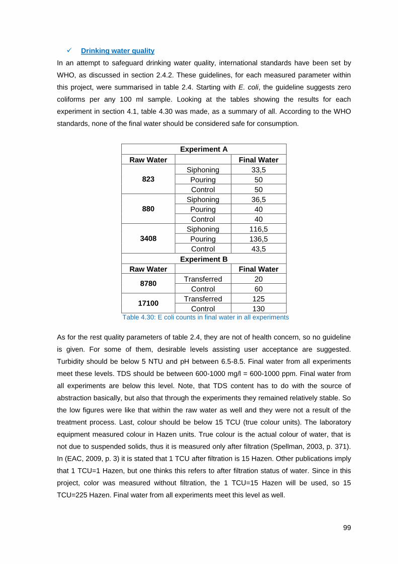
99

Drinking water quality

In an attempt to safeguard drinking water quality, international standards have been set by

WHO, as discussed in section 2.4.2. These guidelines, for each measured parameter within

this project, were summarised in table 2.4. Starting with E. coli, the guideline suggests zero

coliforms per any 100 ml sample. Looking at the tables showing the results for each

experiment in section 4.1, table 4.30 was made, as a summary of all. According to the WHO

standards, none of the final water should be considered safe for consumption.

Experiment A

Raw Water Final Water

823

Siphoning 33,5

Pouring 50

Control 50

880

Siphoning 36,5

Pouring 40

Control 40

3408

Siphoning 116,5

Pouring 136,5

Control 43,5

Experiment B

Raw Water Final Water

8780 Transferred 20

Control 60

17100 Transferred 125

Control 130 Table 4.30: E coli counts in final water in all experiments

As for the rest quality parameters of table 2.4, they are not of health concern, so no guideline

is given. For some of them, desirable levels assisting user acceptance are suggested.

Turbidity should be below 5 NTU and pH between 6.5-8.5. Final water from all experiments

meet these levels. TDS should be between 600-1000 mg/l = 600-1000 ppm. Final water from

all experiments are below this level. Note, that TDS content has to do with the source of

abstraction basically, but also that through the experiments they remained relatively stable. So

the low figures were like that within the raw water as well and they were not a result of the

treatment process. Last, colour should be below 15 TCU (true colour units). The laboratory

equipment measured colour in Hazen units. True colour is the actual colour of water, that is

not due to suspended solids, thus it is measured only after filtration (Spellman, 2003, p. 371).

In (EAC, 2009, p. 3) it is stated that 1 TCU after filtration is 15 Hazen. Other publications imply

that 1 TCU=1 Hazen, but one thinks this refers to after filtration status of water. Since in this

project, color was measured without filtration, the 1 TCU=15 Hazen will be used, so 15

TCU=225 Hazen. Final water from all experiments meet this level as well.

100

The applicability of these guidelines and especially the E. coli one, has been widely debated,

as presented in section 2.4.2. To overcome that debate, comparing the E. coli levels with the

infectious dose is more practical. Indeed for E. coli, for the commonest type-ETEC this can be

108-10

10 organisms, while for EHEC (Enterohaemorrhagic) 100-10

6 (Hunter, 2003, p. 67-68).

Three issues can be discussed on that. First, the infectious dose is expressed in number of

organisms within the infected individual and not in cfu/100 ml, as measured in the laboratory.

When counting bacteria in the lab, colony forming units (cfu) are distinguished. The

assumption is that each viable bacteria will form a discrete colony, but in reality in each colony

many more bacteria can be present (Reynolds et al. 2005, p. 1). With that assumption, 1

cfu/100 ml can be simplified into 1 bacterium/100 ml. Assuming again that the average

drinking water quantity is consumed, which is 2 lcd (see section 2.4.1), 2 litres=2000ml. Taking

the larger figure from table 4.30, this is 136 cfu/100 ml or 136 bacteria/100 ml, according to the

first assumption and 2720 bacteria/2 litres. Second issue is that it is not certain which type of E.

coli is found within the water each time. If it is the common type, the number of 2720 bacteria

is way far from the infectious dose. However, if it is the more aggressive type, there is a

chance of infection from most of the samples. Thirdly, drinking water isn't the only pathway for

bacteria to enter the human system. Even if the previous assumptions can be accepted up to

a point, it would be an oversimplification to assume that no other coliforms enter the body.

This is one of the reasons that WHO guidelines are so strict, according to one’s judgment.

Last, comparing the results form table 4.30 with the levels of safety presented in table 2.5,

most samples fall in the third category of intermediate risk (11-100 cfu/100ml), characterized

as polluted, but that can still be consumed as it is, if no treatment is available. This is even

characterized as moderately good quality (Feachem et al. 1983, p. 210).

As concluded in section 2.4.2 as well, apart from guidelines and standards, the key idea is that

of water quality improvement. “A moderately effective water treatment that raises the levels of

the most important quality parameters – those that affect health – without meeting all the

parameters and standards” may be perceived as an improvement in water quality (Heber,

1985, p. 13). Since all measured parameters in every experiment – not only those affecting

health, no matter the initial variables or the final result, has been improved, treatment of water

with the three-pot system is undeniable.

SHTEFIE approach

In an attempt to analyse the three-pot method in a more holistic way, the SHTEFIE criteria,

adopted from (Parr et all, 1999, p. 66), were kept in mind throughout the project. SHTEFIE

stands for: Social, Health, Technological, Economic, Financial, Institutional and Environmental

101

criteria. These issues have already been mentioned within the previous chapters, but

summarizing here to trigger further discussion:

- Social: The three-pot system is simple and easy to use, with no special skills required and

very low cost. That makes it suitable for almost all social groups, therefore promoting equity.

The user can have control of his own water treatment with local material, therefore promoting

self-reliance. It doesn’t require much time from the user, since the treatment is a natural self-

purification mechanism of water, therefore he can spend this time more productively. It can be

used both in emergencies and development. It addresses most acceptability parameters within

the water quality and manages to improve significantly all of them, therefore the user can be

willing to adopt it. The treatment itself doesn’t seem socially or culturally insulting in any way,

since it is using simple household material. Of course, acceptability in water quality and on a

social level is subjective and cannot be guaranteed.

- Health: The three-pot reduces E. coli significantly. The reduction depends on many variables,

but it can be basically controlled by prolonging the days of retention. Any water improvement,

supports health of people. However, the three-pot hasn’t been tested for other types of

pathogens as well. Issues of algal or bacteria growth need to be taken into consideration when

longer retention time is practiced.

- Technological: The “technology” involved in the three-pot system is simple and easy to use.

There is no need for electrical power or chemicals. The use of 1-2-3 pots and of any kind of

vessels, makes it flexible. Collection, treatment, storage and consumption of water can all be

addressed with the same vessels. The materials can be found locally and basically these are

the containers involved. In the case where siphoning is practiced, some sort of siphon has to

be available, but the system works without it as well. For all that the system can be

characterized adoptable and sustainable. The use of siphon may protect the system from

misusing it, but it is quite slower than pouring. On the other hand if the volume of water is too

large to be lifted, siphoning is opted. Too large volumes can be divided into smaller containers

alternatively, but that would create a space problem within a household if 3 pots are used and

not one.

- Economic: Local materials, even found within the household, don't require supporting the

market supply chains, which is a common problem when material need to be imported in a

country and if not addressed, water treatment and supply can be interrupted. Adopting the

three-pot method which is low cost and having practically no recurrent costs, doesn't burden

the economy of the household. Not much time is required from the user, which makes three-

pot economic in that sense. The overall health improvement, leads indirectly to improvement

of the house economy and one step further, of the local and country economy.

- Financial: The containers, if not already within the household, are low cost. This capital

investment is small and the recurrent costs are practically zero. Practically, implies that there

can be a minor cost for periodical cleaning of the pots and replacing the pots when their

102

lifespan is over. No power or purchase of chemicals is needed. Siphon can be one more small

additional cost.

- Institutional: The three-pot needs to regarded as an option of the whole idea of HWTS, since

it practically treats water at a household level and stores it safely. It can be used by

stakeholders to scale up interventions on safe water, either alone or as part of another water

treatment procedure. Field research is required to support the system as well. Since it can be

practiced with any containers, market rules do not apply on it, therefore self-reliance is further

promoted.

- Environmental: The improvement in health, improves the overall environment. The system

itself, doesn't require chemicals, power or any constructions. It is a process practiced by

nature anyway. The environmental impact therefore of the system cannot be negative. Only

the material of the container needs to be considered, when disposed of. In cases of plastic, it

is not friendly to the environment, but on the other hand, durability of plastic pots, give them a

wide lifespan, so the amount of plastic disposed from the three-pot system cannot be that

large.

These issues can characterize the three-pot system as an overall sustainable option, able to

support the development of a household and consequently of an area and of a country in a

larger scale. That fact should place the three-pot system among the rest HWT options. The

simple and low-cost implementation of the three-pot system, makes it suitable for scaling up

very quickly, therefore it is included in the emergency water treatment options as well.

However, it should not be confused that this is its only suitable application.

4.4 Limitations

4.4.1 Limitations of the three-pot system

There are some limitations within the three-pot system, previously discussed within the

chapters. They are worth re-mentioning here as issues one should be careful of when

practicing or studying the system.

The three-pot improves all the studied water quality parameters and removes significantly the

E. coli counts. However, the improvement rises more when the retention time is larger. It is

safer to practice the method for three-days, thus called three-pot, before consumption of water.

Even that though, cannot guarantee perfect results. The reduction rates are largely dependant

on the initial loading. Unfortunately, this figure is not easy to be known on a household

everyday level. Field tests or sanitary surveys are conducted by officials to identify that level

on an everyday local scale. Basic principles borrowed from sanitary surveys can be passed to

the users through training for safer practice of the three-pot as well. Another limitation rising

from longer retention times, when water is decanted and the bottom volume is thrown away, is

103

that the water left for consumption finally is smaller than the initial water collected. That needs

to be taken into consideration when calculating the household water needs.

Another issue is that water near the surface is of better bacteriological quality than that on the

bottom. Users should be aware of that in order not to abstract water from taps placed near the

bottom of the container, if placed there. Also, they should be careful not to decant all the water

from one container to the other, including the bottom layer. This needs to be thrown away.

When pouring is practiced, the pot should be tipped over gently, so as not to disturb the

sediments and re-suspend them, thus transfer them in the next pot. Additional concern in that

sense, is that how much water will be left behind depends on the user’s eyesight or preference.

There can’t be a standard volume to be given as guidance, since it has to do with the loading

of the suspended solids each time. Extra caution should be given when water “seems” clean

because of the absence of suspended solids. Users need to be aware that pathogens are not

seen with naked eye, so water needs to follow the three-pot system anyway.

Moreover, basic hygiene knowledge needs to be given if the users are not already aware of it.

These are typical issues concerning every HWTS option. Vessels and the siphon, if used,

need periodic cleaning. A lid prevents recontamination. Any utensil dipped in the consumable

water needs to be clean as well. Users should avoid putting their hands in the water.

4.4.2 Limitations of the project

As in any task, here as well there were some factors limiting the project, worth to mention, so

as to be addressed in any future similar work. Research method and personal calculations or

observations, should always be considered as the first limitation. Even after careful

consideration, there always seem to be issues or mistakes, not properly realized and

addressed.

The idea behind the experiments was for them to be done as close to real field conditions as

possible, thus stream water was collected. However, this produced too varying quality

parameters, making results less easy to be compared. Instead, artificial water could be

created, with better control over the parameters, but since there was a chance of bacteria

acting differently in each case, the option of natural water was made.

In that sense, experiment A was repeated three times, but the initial water quality was different

each time, although not intended. However, this random fact was exploited so as to

understand better how bacteria act when they exist in different populations. Another issue in

experiment A, was that the initial quality for each three-pot system was measured for two

samples and assumed the same for the rest. That was due to time constrains within the

104

laboratory working hours. That wasn’t repeated in experiment B, where one was given

authorization to work above the official opening hours and days of the laboratory, thus each

system was counted separately from the beginning. Last one more issue, addressed only in

experiment B again, was the volume of water left in the previous pot after every decanting

procedure. In experiment A, it was done approximately by looking at the sediments, thus the

water transferred differed in volumes (see appendix 8.1). In experiment B, the volume

transferred was kept constant by measurement and not by eyesight. Even when that volume

was decided to change, that was applied to all systems at once.

Major limitation within this project was the issue with the suspended solids filters, basically on

experiment A. As explained in methodology, when the loading isn't that big, higher quality

filters are needed to capture the small differences in weight, but these were not available

within the laboratory. On top of that, packets of filters already open, gather humidity from the

atmosphere, adding weight to the filters. Then when the filters are placed in the oven, filtered

water dries up along with the humidity. Since the suspended solids loading was minor and

didn't contribute much on the filter’s weight, the result was having lighter filters, even with the

solids on them. That was just recording the loss of humidity actually. Thus the suspended

solids were faulty and couldn’t be trusted. In experiment B, this was addressed, by pre-wetting

and drying the filters and keeping them in the oven until use, so as not to collect air humidity.

Last major procedural limitation was the syringe issue. The syringe was chosen so as to

collect water from any depth without causing disturbance. This removable appliance was also

opted to any permanent option of abstraction like taps, since edges can collect settled solids

and bacteria more easily. Since the samples were relatively small (10 ml), there was the

concern of these samples capturing the water quality of the particular edge and not of the

whole container. The syringe was decided to collect water from the same point within the

bucket, for repetition ease. For the samples taken straight from the bottom, the syringe

seemed to clear off the area, so again the water quality of the particular spot, didn't seem to

represent the whole container. Once more the results couldn’t be trusted.

In general, sampling from any point within settling water is random, since settlement is

affected by many variables, which cannot be controlled in total. In that sense, only large

number of experiments and repetitions can provide a clear image of the situation in such a

microscopic level. Therefore, more laboratory research is advised, since there doesn't seem to

be enough on such a small scale level, like the three-pot system. Field studies should be

going along laboratory studies, as they are supplementary and give useful feedback to one

another. Only that combination can produce reliable results and promote actual development

in the research area.

105

4.5 Review

The present chapter presented the results and attempted to comment and promote useful

discussion on them. Reviewing the outcome from it, one could summarize in this section in

shorter version.

Looking at the research questions:

Three days of treatment are advised to reach 90% bacteria reduction no matter the initial

loading. Siphoning is slightly more effective than pouring in bacteria reduction, especially at

smaller retention times, but doesn't assist aeration that much. Practical issues of efficiency rise

as well with the siphon option. Surface water is indeed of better quality than that of the bottom.

One pot produces only slightly worse quality water, but it is not advised because aeration

doesn't occur and also for acceptability issues. All of the differences found within the systems

seem to be minimized when more retention time is allowed. The longer the retention time, the

better the water quality is the key rule for one to remember.

Overall, the three-pot system improves all measured parameters of water quality within this

project. This means that it provides undoubted water treatment. Being practiced on a

household level along with safe storage, attributes the title of HWTS. The three-pot system

produces higher quality water than simple sedimentation, because aeration plays an important

role. The exact purification mechanism or which parameters play more significant role than

others is difficult to be concluded, since the relationships between the variables are

complicated and even minor changes to the researcher’s eye seem to have major impact on a

microscopic level.

Effective and efficient are two different issues. The effectiveness was tested, but the efficient

could only be discussed. Measuring efficiency is more difficult, since more abstract and

subjective term. Field surveys need to be done on the three-pot system to understand efficient

issues further.

106

5.0 Recommendations

5. 1 Recommendations on the three-pot system

Looking at the limitations of the three pot system (section 4.4.1), consequently, some

recommendations could be given for maximizing the benefits of that type of treatment.

The most important one, which safeguards that all water quality parameters will have

improved is allowing at least three days of retention time. As previously repeated, the longer

the retention time, the better. Moreover, It is advised that users abstract water from the

surface when they need to consume it, since it is of better bacteriological quality. Decanting

water should be done gently, so as not to disturb and re-suspend the sediments and minimize

the possibilities of carrying them along with the transferred water in the next pot. Always a

volume of water should be left behind to be thrown away. These two practices need to be

followed even when the water “seems” clean from suspended solids, because pathogens are

not visible, but they may still exist in the bottom of the water. The use of a clean cloth initially,

when the raw water is poured into the first pot, could hold larger suspended matter visible to

the naked eye.

Moreover, basic hygiene knowledge needs to be given if the users are not already aware of it.

The vessels and the siphon, if used, need periodic cleaning. That can be done with boiling

water and/or some sort of bleach solution. A safely tight lid always prevents recontamination.

Any utensil dipped in the consumable water needs to be clean as well. Users should also

avoid putting their hands in the water.

It is always difficult to safeguard that all users will be aware of these issues, therefore practice

the treatment correctly. There is always the unknown factor of unpredictable human behaviour,

that could cancel or minimize the benefits of the treatment. The best way to safeguard the

benefits, even when users are not fully aware of the reasons, is to promote the use of three

pots, where water is being decanted each day. This way water will remain in the pots for at

least three days, which has been proved to give the best possible results in the shorter period

of time for all systems. Three days are easy to remember, because they follow the name of

the three-pot system. However, it has been proved within this project (see section 4.2) that

even when three days or three pots are not practiced, less days and less pots still provide

water treatment. Any improvement in the water quality parameters, even if it is smaller than

the maximum that could be achieved, should not be neglected, since it is still an improvement.

Last recommendation would be on how the three-pot system could be scaled up. As

mentioned earlier, all HWT options are promoted and researched further, because institutions

and companies found opportunities through them to launch new products in the market. The

107

three-pot system on the other hand, consisting of any three containers available, doesn't give

many opportunities for market expansion. The only HWT option which managed to be

recognised and was scaled up without dealing with market terms was solar disinfection, known

by the name SODIS. SODIS is practiced basically with the use of transparent bottles, mainly

plastic. Therefore, it was scaled up mainly by promoting the method and not the materials

needed for its implementation, like in the rest HWT options. Studying the case of SODIS, one

could see how the three-pot technique could be promoted in a similar way.

5. 2 Recommendations for future projects

In the present section, an attempt to generate some ideas for prospective researchers will be

done. These could be followed as they are presented or even better, just trigger their thinking

and assist them in coming up with some genuine ones.

To start with, looking at the limitations in section 4.4.2, since it was decided to conduct the

experiments with natural water so as to have more realistic conditions, one could suggest

testing the three-pot system with artificial water replicating the natural one. This way it will be

easier to have control over the water quality parameters and each time change strictly only

one variable, so as to have a more clear picture of the role it plays. Water with exclusively

artificially cultivated E. coli is worth to be tested, since there have been studies suggesting the

different reaction they have compared to the natural ones. Also, within this project, there was

an indication that the sample with the artificial added bacteria, showed different reaction as

well (see section 4.2.1). Whether this has to do with these bacteria dying faster, since they are

less resilient as previously suggested or whether because they settle less efficiently, since

they are not attached to any solids, as natural bacteria, needs further research. In (Feachem

et al. 1983, p. 60) it is suggested that in clean water bacteria may survive longer, since there is

no competition or predation by other microorganisms, but on the other hand, some pathogens

survive longer in dirty water, because they find protection attached to the solids. As a general

rule though, it is said that “death rates are higher in natural waters with an active biological

population, than in sterilized, filtered or other “dead” water (Feachem et al. 1983, p. 209). Last

point to mention from section 4.4.2, is that care with any procedural and laboratory mistakes,

is always recommended, to avoid limitations like the suspended solids or the syringe issue.

Next, looking at the design characteristics of the three-pot system (section 2.2.3), one could

recommend future issues worth to be further researched. These could be:

1. a. Inlet water quality → alter the parameters to any extent, either alone or in combination.

More interesting would be the suspended solids, since they play an important role in

sedimentation, therefore in the purification mechanism of the three-pot system. Comparing

characteristically, a sample with suspended solids and a sample completely free of it, both

108

with the same bacteria loading, would be really valuable. Suspended matter seem to be

regarded negatively when present in water, but in case of sedimentation it can be beneficial in

a sense. Another essential test would be testing the effectiveness of the three-pot system with

other pathogens apart from E. coli.

b. Inlet water quantity → alter the quantities of the water treated, above the 10 l chosen to

be tested here. It would be interesting to see if the purification mechanism depends on the

volume of the water body. A comparison between smaller quantities with larger sedimentation

tanks could be done, so as to test if the same theories apply to water, no matter the scale.

c. Use of cloth or not at the inlet point → compare the difference in the purification

mechanism of the three-pot when a cloth is used at the inlet point. That leads back to the idea,

whether the presence of more suspended solids is beneficial or not.

2. a. Size of vessel → that leads back to the water quantity recommendations, since the size

depends on the quantity.

b. Shape of vessel → testing the three-pot system in different shaped vessels, using same

quality water, could conclude on whether this can alter in any case the purification mechanism.

The presence of corners characteristically, is claimed to facilitate the bacteria colonies to

attach and grow (Oxfam, 2008, p. 4).

c. Material of vessel → testing the three-pot system in different materials of vessels, using

same quality water, could conclude on whether this can alter in any case the purification

mechanism again. Different materials are reported to alter the water parameters like pH,

conductivity, TDS and therefore the bacteria die-off rates (Qi, 2007). Interesting suggestion by

the supervisor was the use colloidal silver, since in the case of ceramic pot filters, enhanced

with this metal, it has been reported to improve the microbiological effectiveness (Rayner,

2009).

d. Rest vessel characteristics (colour, opening, lid, handle, tap) → different coloured vessels

using the same quality water, could test whether the presence of light could have an effect on

the purification mechanism. Light in cases of solar disinfection, where the containers are

transparent is reported to kill the bacteria, but on the other hand, light assists algal growth as

well.

e. Number of pots in use → this was already addressed within this project (see section

4.2.5), but it can always be repeated with different parameters for confirmation.

f. Retention time (days of storage) → again this was already addressed within this project

(see section 4.2.2), but it can always be repeated with different parameters for confirmation.

Testing the difference on an hour scale not on a day scale could be interesting as well.

3. a. Method of decanting → again this was already addressed within this project (see section

4.2.3), but it can always be repeated with different parameters for confirmation. Stirring up the

109

transferred water, before allowing it to settle for a day, can test if that assists flocculation of

bacteria, therefore helping their sedimentation and improve the water quality further.

b. Point of abstraction → this was attempted to be addressed for surface and bottom water

(see section 4.2.4). Measurements along the depth of the water column, especially in larger

volumes of water, could provide helpful information on how sedimentation differs with depth.

Last, looking at the “multi-barrier approach” idea, where the various HWTS options should be

combined for better results in the pathogen removal efficiency (WHO, 2011, p. 143), some

more suggestions can be given. Adding different coagulants in the raw water or Using other

disinfection options like clay ceramic balls, chemical solutions and so forth, to test their

contribution on the three-pot system could produce various new theories for testing. The key

idea is to test the contribution of any other method to the three-pot system and not the other

way around. Testing the contribution of the three-pot system on other HWTS options, could

support arguments that place the three-pot system as a pre-treatment option only. Besides,

the overall contribution of the project is to give appropriate recognition to the three-pot system

as a HWTS option and not just as a pre-treatment one. Only then users could adopt it in a

larger extent and allow to the three-pot system to play an active role to the universal goal of

improving the quality of drinking water.

In general, additional research is always advised, especially in the HWTS options which are

relatively recent and on the three-pot system in particular, as this scale of treatment hasn’t

been researched (see section 2.3.1). In that sense, even if the experiments of this project are

repeated with not many alterations, it could be a good chance for the results to be confirmed

or not. Field studies are always recommended along with laboratory experiments for more

realistic results and for grasping efficiency issues better.

110

6.0 Conclusions

The present research aimed at testing the effectiveness of the three-pot water treatment

system by answering five particular research questions (see section 1.2.3). Repeating here

the review of the results (section 4.5):

Three days of treatment are advised to reach 90% bacteria reduction no matter the initial

loading. Siphoning is slightly more effective than pouring in bacteria reduction, especially at

smaller retention times, but doesn't assist aeration that much. Practical issues of efficiency rise

as well with the siphon option. Surface water is indeed of better quality than that of the bottom.

One pot produces only slightly worse quality water, but it is not advised because aeration

doesn't occur and also for acceptability issues. All of the differences found within the systems

seem to be minimized when more retention time is allowed. The longer the retention time, the

better the water quality is the key rule for one to remember.

Overall, the three-pot system improves all measured parameters of water quality within this

project. This means that it provides undoubted water treatment. Being practiced on a

household level, attributes the title of HWT. The three-pot system produces higher quality

water than simple sedimentation, because aeration plays an important role. The exact

purification mechanism or which parameters play more significant role than others is difficult to

be concluded, since the relationships between the variables are complicated and even minor

changes to the researcher’s eye seem to have major impact on a microscopic level.

The three-pot system is a simple, low-cost solution, easy to operate and maintain, which

makes it efficient for the user. It basically exploits the self-purification processes that occurs in

natural water bodies. Moreover, it can be practiced with any containers within the household.

These features makes it able to be implemented without supply chains and market rules.

Therefore, it promotes the user’s self-reliance in a natural way. All these, can characterize the

three-pot system a sustainable solution able to support the development of a household and

consequently of an area and of a country in a larger scale. The simple and low-cost

implementation of the three-pot system, makes it suitable for scaling up very quickly, therefore

it is included in the emergency water treatment options as well. However, it should not be

confused that this is its only suitable application.

Note though that effective and efficient are two different issues. The effectiveness was tested,

but the efficiency could only be discussed. Measuring efficiency is more difficult, since more

abstract and subjective term. Field surveys need to be done on the three-pot system to

understand efficient issues further. Besides, field and laboratory research should be

conducted in parallel, giving useful feedback to one another. This is even more necessary on

111

the relatively new area of HWT options and on the three-pot system in particular, which hasn't

been tested before.

Looking at figure 1.1, in an attempt to depict the project’s contribution, by including the three-

pot system in the HWT “family”, one could say that the long-term goal of development can be

further assisted. However, if some people are not convinced and still perceive it as a pre-

treatment or an emergency option, the present research can be of use to them as well, as a

record of the magnitude of treatment provided by the system, regardless of where it is used.

In that sense, the three-pot can be seen as an “improved” sedimentation option. It has mainly

the same principles with sedimentation, but aeration rises the positive effects further.

Moreover, by suggesting the three-pot procedure, where water is being decanted each day,

one safeguards the results of sedimentation and maximizes the health benefits for the user.

This way water will remain in the pots for at least three days, which has been proved to give

the best possible results in the shorter period of time for all systems. By naming the method

“three-pot”, the user will indirectly be lead to allow these three days to pass and it will be

easier to remember. It is better to establish that name for the method then as a way of setting

indirect guidelines for the sedimentation option.

However, it has been proved within this project (see section 4.2) that even when three days or

three pots are not practiced, less days and less pots still provide water treatment. Any

improvement in the water quality parameters, even if it is smaller than the maximum that could

be achieved, should not be neglected, since it is still an improvement. That should be the

general idea when considering if treatment options should be recognised or not. “A moderately

effective water treatment that raises the levels of the most important quality parameters –

those that affect health – without meeting all the parameters and standards” may be perceived

as an improvement in water quality (Heber, 1985, p. 13).

“Appropriate technology doesn’t imply modern and sophisticated technology versus basic

technology, but on the contrary, out of a wide spectrum of possible methods, materials and

systems, a choice must be made that is specifically tailored to a particular place” (Heber, 1985,

p. 6). In that sense, the three-pot, could be an appropriate solution for many cases. Besides, it

is wiser not to argue about it, but deal with the difficult issue of safe drinking water and

consequently with the long-term goal of development from as many angles as possible.

112

7.0 References

ASHBOLT, J.N., 2004. Microbial Contamination of Drinking Water and Disease Outcomes in

Developing Regions. Toxicology: 198 (1-3), p. 229-238. [viewed: June 2012]. Available from:

http://www.researchgate.net/publication/8568022_Microbial_contamination_of_drinking_water

_and_disease_outcomes_in_developing_regions

BARTRAM, J. and BALANCE, R., 1996. Water Quality Monitoring – A Practical Guide to the

Design and Implementation of Fresh Water Quality Studies and Monitoring Programmes.

London: UNEP/WHO. [viewed: June 2012]. Available from:

http://www.who.int/water_sanitation_health/resourcesquality/waterqualmonitor.pdf

BEEMAN, N., 1931. The Effect of Hydrogen-Ion Concentration Upon the Sedimentation of

Clay. Journal of the American Ceramic Society: 14 (1), p. 72-87.

CAIRNCROSS, S. and FEACHEM, R., 1993. Environmental Health Engineering in the Tropics.

2nd

ed. Chichester: Wiley Publications

CAIRNCROSS, S., 1993. WELL Factsheet: Bacteriological Testing of Water. Loughborough:

WELL Publications. [viewed: June 2012]. Available from:

http://www.lboro.ac.uk/well/resources/fact-sheets/fact-sheets-htm/btw.htm

CAIRNCROSS, S., HUNT, C., BOISSON, S., BOSTOEN, K., CURTIS, V. and FUNG, I., 2010.

Water, Sanitation and Hygiene for the Prevention of Diarrhoea. International Journal of

Epidemiology: 39 (1), p. 193-205. [viewed: June 2012]. Available from:

http://ije.oxfordjournals.org/content/39/suppl_1/i193.full

CAMPBELL, S., 1983. The Home Water Supply: How to Find, Filter, Store and Conserve It.

US: Storey Communications

CAWST (Centre for Affordable Water and Sanitation Technology), 2010. Household Water

Treatment and Safe Storage Factsheet: Settling. Calgary: CAWST. [viewed: June 2012].

Available from:

http://media.greennexxus.com/wasrag/articles_of_interest/water_supply/Water_treatment/Hou

sehold_Treatment_Systems/CAWST_Household_Water_Treatment_Safe_Storage_Source_P

rotection.pdf

CDC (Centre for Disease Control and Prevention), 2000. Safe Water Systems for the

Developing World: A Handbook for Implementing Household-Based Water Treatment and

113

Safe Storage Projects. Atlanta: CDC. [viewed: June 2012]. Available from:

http://www.cdc.gov/safewater/PDF/SWS-for-the-developing-world-manual.pdf

CIWEM (Chartered Institution of Water and Environmental Management), 2012. Population,

industrialization and climate change exacerbate global water shortages. CIWEM Business

Briefing: 17 (5), p. 1.

CLASEN, T., 2009. Scaling Up Household Water Treatment Among Low-Income Populations.

Geneva: WHO. [viewed: June 2012]. Available from:

http://whqlibdoc.who.int/hq/2009/WHO_HSE_WSH_09.02_eng.pdf

CLASEN, T., HALLER, L., WALKER, D., BARTRAM, J. and CAIRNCROSS, S., 2007 (b).

Cost-Effectiveness of Water Quality Interventions for Preventing Diarrhoeal Disease in

Developing Countries. Journal of Water and Health: 05 (4), p. 599-608. viewed: June 2012].

Available from: http://www.iwaponline.com/jwh/005/0599/0050599.pdf

CLASEN, T., SCHMIDT, W. P., RABIE, T, ROBERTS I., and CAIRNCROSS, S, 2007 (a).

Interventions to Improve Water Quality for Preventing Diarrhoea: Systematic Review and

Meta-Analysis. British Medical Journal: 334 (7597), 782-792. [viewed: June 2012]. Available

from: http://www.bmj.com/highwire/filestream/357645/field_highwire_article_pdf/0.pdf

CONANT, J., 2005. Water for Life – Community Water Security. California: The Hesperian

Foundation. [viewed: June 2012]. Available from:

http://www.unwater.org/downloads/Water_EN.pdf

DAVIS, J. and LAMBERT, R., 2002. Engineering in Emergencies: A Practical Guide for Relief

Workers. 2nd

ed. London: ITDG Publishing

DeVEER, T., 2002. Chapter 24: Water Supply in disasters and emergencies. In: SMET, J. and

WIJK, C., 2002. Small Community Water Supplies, Technology, People and Partnership.

Hague: International Water and Sanitation Centre. [viewed: June 2012]. Available from:

http://www.samsamwater.com/library/TP40_24_Water_supply_in_disasters_and_emergencies

.pdf

DFID (Department for International Development), 1998. Guidance Manual on Water Supply

and Sanitation Programmes. Loughborough: WEDC, Loughborough University

114

EAC (East African Community), 2009. East African Draft Standard: Potable Water-

Specification. Arusha: EAC. [viewed: June 2012]. Available from: http://www.eac-

quality.net/fileadmin/eac_quality/user_documents/3_pdf/EAS_12-2010__Potable_water.pdf

ENSSLIN, C.H., 2005. Rainwater Tanks in Series. Unpublished MSc Thesis. Loughborough:

WEDC, Loughborough University

EPA (Environmental Protection Agency), 1997. Volunteer Stream Monitoring: A Methods

Manual. Washington: EPA. [viewed: June 2012]. Available from:

http://water.epa.gov/type/rsl/monitoring/upload/2002_08_13_volunteer_stream_stream.pdf

FEACHEM, R.G., BRADLEY, D., GARELICK, H. and MARA, D.D., 1983. Sanitation and

Disease: Health Aspects of Excreta and Wastewater Management. Washington: World Bank.

FEWTRELL, R.B., KAY, D., ENANORIA, W., HALLER, L. and COLFORD, J.J.M., 2005. Water,

Sanitation and Hygiene Interventions to Reduce Diarrhoea in Less Developed Countries: a

Systematic Review and Meta-Analysis. Lancet Infectious Diseases: 5 (1), 42-52. [viewed:

June 2012]. Available from:

http://www.sciencedirect.com/science/article/pii/S1473309904012538

GALVIS, G.C., 2002. Chapter 12: Water Treatment. In: SMET, J. and WIJK, C., 2002. Small

Community Water Supplies, Technology, People and Partnership. The Hague: International

Water and Sanitation Centre. [viewed: June 2012]. Available from:

http://www.irc.nl/content/download/128534/350994/file/TP40_12%20Water%20treatment.pdf

HARVEY, P., 2007. WELL Factsheet: Field Water Quality Testing in Emergencies.

Loughborough: WELL Publications. [viewed: June 2012]. Available from:

http://www.lboro.ac.uk/well/resources/fact-sheets/fact-sheets-

htm/WQ%20in%20emergencies.htm

HEBER, G, 1985. Simple Methods for the Treatment of Drinking Water. Eschborn: Vieweg

HETV (Health Education to Villages), 2012 (a). Safe Water Systems for the Developing World:

A Handbook for Implementing Household-Based Water Treatment and Safe Storage Projects.

Atlanta: CDC. [viewed: June 2012]. Available from:

http://hetv.org/resources/safewater/manual/1_toc.htm

http://www.sciencedirect.com/science/article/pii/S1473309904012538

http://hetv.org/resources/safewater/manual/1_toc.htm

115

HETV (Health Education to Villages), 2012 (b). Alternative Water Treatment Technologies. In:

Safe Water Systems for the Developing World: A Handbook for Implementing Household-

Based Water Treatment and Safe Storage Projects. Atlanta: CDC. [viewed: June 2012].

Available from: http://hetv.org/resources/safewater/manual/alt_water.htm

HOUSE, S., INCE, M., and SHAW, R., 1999. Water-Quality or Quantity? Technical Brief 52. In:

SHAW, R., 1999. Running Water: More Technical Briefs on Health, Water and Sanitation.

London: IT Publications. [viewed: June 2012]. Available from:

http://www.lboro.ac.uk/well/resources/technical-briefs/52-water-quality-or-quantity.pdf

HOWARD, G. and BARTRAM, J., 2003. Domestic Water Quantity, Service Level and Health.

Geneva: WHO. [viewed: June 2012]. Available from:

http://www.who.int/water_sanitation_health/diseases/WSH03.02.pdf

HOWARD, G., 2002., Water Quality Surveillance – A Practical Guide. Loughborough: WEDC,

Loughborough University. [viewed: June 2012]. Available from: http://www-

esd.worldbank.org/esd/ard/groundwater/pdfreports/WQsurveillance_practical_Gde.pdf

HWTS NETWORK (Household Water Treatment and Safe Storage Network), 2007.

Combating Waterborne Disease at the Household Level. Geneva: WHO. [viewed: June 2012].

Available from:

http://www.wsscc.org/sites/default/files/publications/who_combating_waterborne_disease_at_

household_level_20.pdf

HUANG, Y., 2006. A practical Examination of Water Quality: Studying the Burleigh Brook.

Unpublished MSc Thesis. Loughborough: WEDC, Loughborough University

HUISMAN, L. and WOOD, W.E., 1974. Slow Sand Filtration. Geneva: WHO. [viewed: June

2012]. Available from: http://whqlibdoc.who.int/publications/9241540370.pdf

HUNTER, P., 2003. Drinking Water and Diarrhoeal Disease due to Escherichia coli. Journal of

Water and Health: 01 (02), p. 65-72. [viewed: June 2012]. Available from:

http://www.iwaponline.com/jwh/001/0065/0010065.pdf

IFRC (International Federation of Red Cross and Red Crescent Societies), 2008. Household

Water Treatment and Safe Storage in Emergencies: A Field Manual for Red Cross/Red

Crescent Personnel and Volunteers. Geneva: IFRC. [viewed: June 2012]. Available from:

http://www.ifrc.org/Global/Publications/disasters/142100-hwt-en.pdf

http://hetv.org/resources/safewater/manual/alt_water.htm

116

IVES, K., 2002 (a). Chapter 15: Sedimentation. In: SMET, J. and WIJK, C., 2002. Small

Community Water Supplies, Technology, People and Partnership. Hague: International Water

and Sanitation Centre. [viewed: June 2012]. Available from:

http://www.irc.nl/content/download/128537/351003/file/TP40_15%20Sedimentation.pdf

IVES, K., 2002 (b). Chapter 14: Coagulation and Flocculation. In: SMET, J. and WIJK, C.,

2002. Small Community Water Supplies, Technology, People and Partnership. Hague:

International Water and Sanitation Centre. [viewed: June 2012]. Available from:

http://www.irc.nl/content/download/128536/351000/file/TP40_14%20Coagulation%20and%20fl

occulation.pdf

IVES, K., 2002 (c). Chapter 13: Aeration. In: SMET, J. and WIJK, C., 2002. Small Community

Water Supplies, Technology, People and Partnership. Hague: International Water and

Sanitation Centre. [viewed: June 2012]. Available from:

http://www.irc.nl/content/download/128535/350997/file/TP40_13%20Aeration.pdf

JONES, J., 1997. Global Hydrology: Process, Resources and Environmental Management.

Essex: Pearson Publications

KAYAGA, S. and REED, B, 2011. Emergency Treatment of Drinking Water at the Point of Use.

Technical Notes on Drinking-Water, Sanitation and Hygiene in Emergencies No. 5. Geneva:

WHO. [viewed: June 2012]. Available from:

http://www.who.int/entity/water_sanitation_health/publications/2011/tn5_treatment_water_en.p

df

KOLLING, G.L. and MATTHEWS, K.R., 2001. Examination of Recovery In Vitro and In Vivo of

Nonculturable Escherichia coli O157:H7. Applied Environmental Microbiology: 67(9), p: 3928–

3933. [viewed: June 2012]. Available from:

http://www.ncbi.nlm.nih.gov/pmc/articles/PMC93111/

KOTLARZ, N., LANTAGNE, D., PRESTON, K. and JELLISON, K., 2009. Turbidity and

Chlorine Demand Reduction Using Locally Available Physical Water Clarification Mechanisms

Before Household Chlorination in Developing Countries. Journal of Water and Health: 07 (3), p.

497-506. [viewed: June 2012]. Available from:

http://www.iwaponline.com/jwh/007/0497/0070497.pdf

117

LeCHEVALLIER, M.W. and AU, K.K., 2004. Water Treatment and Pathogen Control: Process

Efficiency in Achieving Safe Drinking Water. London: IWA Publishing. [viewed: June 2012].

Available from: http://whqlibdoc.who.int/publications/2004/9241562552.pdf

MARA, D. and HORAN, N., 2003. The Handbook of Water and Wastewater Microbiology.

London: Academic Press

MARAIS, G., 1974. Faecal Bacterial Kinetics in Stabilization Ponds. Journal of the

Environmental Engineering Division-Proceedings of the American Society of Civil Engineers:

100, p. 119-139

MINTZ, E., BARTRAM, J., LOCHERY, P. and WEGELIN, M., 2001. Not Just a Drop in the

Bucket: Expanding Access to Point-of-Use Water Treatment Systems. American Journal of

Public Health: 91 (10), 1565-1570. [viewed: June 2012]. Available from:

http://www.cdc.gov/safewater/publications_pages/2001/mintz_2001.pdf

MINTZ, E., REIFF, E. and TAUXE, R., 1995. Safe Water Treatment and Storage in the Home:

A Practical New Strategy to Prevent Waterborne Disease. Journal of the American Medical

Association: 273, 948-935. [viewed: June 2012]. Available from:

http://www.uvm.edu/~bwilcke/reiff.pdf

NATH, K.J., BLOOMFIELD, S. and JONES, M., 2006. Household Water Storage, Handling

and Point-of-Use Treatment. International Scientific Forum on Home Hygiene. [viewed: June

2012]. Available from: http://www.ifh-homehygiene.org/2003/2library/low_res_water_paper.pdf

NCSU (North Carolina State University), 2012. Water Shedss: Dissolved Oxygen. NCSU:

[viewed: June 2012]. Available from: http://www.water.ncsu.edu/watershedss/info/do.html

NOZAIC, D., 2002. Chapter 4: Water Quality and Quantity. In: SMET, J. and WIJK, C., 2002.

Small Community Water Supplies, Technology, People and Partnership. Hague: International

Water and Sanitation Centre. [viewed: June 2012]. Available from:

http://www.samsamwater.com/library/TP40_4_Water_quality_and_quantity.pdf

NWP (Netherlands Water Partnership), 2010. Smart Disinfection Solutions. Amsterdam: NWP.

[viewed: June 2012]. Available from: http://ebookbrowse.com/nwp-2010-smart-disinfection-

solutions-pdf-d116106187

118

OXFAM, 2008. Technical Brief 4: Household Water Treatment and Storage. Oxford: Oxfam.

[viewed: June 2012]. Available from: http://policy-

practice.oxfam.org.uk/publications/household-water-treatment-and-storage-126715

OGUTU, P., GARRETT, V., BARASA, P., OMBEKI, S., MWAKI, A. and QUICK, R., 2001.

Seeking Safe Storage: A Comparison of Drinking Water Quality in Clay and Plastic Vessels.

American Journal of Public Health: 91 (10), p. 1610-1611. [viewed: June 2012]. Available from:

http://www.ncbi.nlm.nih.gov/pmc/articles/PMC1446838/

PARR, J., and SHAW, R., 1999. Choosing an Appropriate Technology. Technical Brief 49. In:


London: IT Publications. . [viewed: June 2012]. Available from:

http://www.lboro.ac.uk/well/resources/technical-briefs/49-choosing-an-appropriate-

technology.pdf

PICKFORD, J., 1991. The Worth of Water. London: ITDG Publishing

QI, S., 2007. Assessing the Impact of Storage Tank Material on Rainwater Quality.

Unpublished MSc Thesis. Loughborough: WEDC, Loughborough University

RAYNER, J., 2009. Current Practices in Manufacturing of Ceramic Pot Filters for Water

Treatment. MSc Thesis. Loughborough: WEDC, Loughborough University. [viewed: June

2012]. Available from: http://www.safewaternow.org/wp-

content/themes/metric/images/study2.pdf

REED, B. and SHAW, R., 1999. Emergency Water Supply. Technical Brief 44. In: SHAW, R.,

1999. Running Water: More Technical Briefs on Health, Water and Sanitation. London: IT

Publications. [viewed: June 2012]. Available from:

http://www.lboro.ac.uk/well/resources/technical-briefs/44-emergency-water-supply.pdf

REED, B., 2005. Technical Notes for Emergencies No. 9: Minimum Water Quantity Needed for

Domestic Use in Emergencies. Geneva: WHO. [viewed: June 2012]. Available from:

http://www.searo.who.int/LinkFiles/List_of_Guidelines_for_Health_Emergency_Minimum_wate

w_quantity.pdf

REED, B., 2011. An Engineer's Guide to Domestic Water Containers. Loughborough: WEDC,

Loughborough University. [viewed: June 2012]. Available from:

http://wedc.lboro.ac.uk/resources/booklets/BK004_WCS_A5_Pages.pdf

http://wedc.lboro.ac.uk/resources/booklets/BK004_WCS_A5_Pages.pdf

119

REED, B., 2012. Unit 1: Introduction to Water Resources. In: Integrated Water Resources

Management. Unpublished MSc Module Notes. Loughborough: WEDC, Loughborough

University

REYNOLDS, J. and FARINHA, M., 2005. Counting Bacteria. Dallas: Richland College. [viewed:

June 2012]. Available from: http://www.biotech.univ.gda.pl/odl/doc/numbers.pdf

RHODES, M., 2008. Introduction to Particle Technology. 2nd

ed. Chichester: Wiley

Publications

ROTTIER, E. and INCE, M., 2003. Controlling and Preventing Disease – The Role of Water

and Environmental Interventions. Loughborough: WEDC, Loughborough University. [viewed:


http://wedc.lboro.ac.uk/resources/books/Controlling_and_Preventing_Disease_-

_Complete.pdf?TARGET=_blank

RUBIO, J., CARISSIMI, E. and ROSA, J.J., 2007. Flotation in Water and Wastewater

Treatment and Reuse: Recent Trends in Brazil. International Journal of Environment and

Pollution: 30 (2), p. 193-207. [viewed: June 2012]. Available from:

http://www.tratamentodeagua.com.br/r10/Lib/Image/art_448227668_Flotation_in_water_and_

wastewater_treatment_and_reuse.pdf

RUFENER, S., MAUSEZAHL, D., MOSLER, H.J., and WEINGARTNER, R., 2012. Quality of

Drinking-Water at Source and Point-of-Consumption: Drinking Cup as a High Potential

Recontamination Risk: A Field Study in Bolivia. Journal of Health, Population and Nutrition: 28

(1), 34-41. [viewed: June 2012]. Available from:

http://www.ncbi.nlm.nih.gov/pmc/articles/PMC2975844/?tool=pubmed

SINGER, S., 2010. Maintenance of the Biosand Filter Explored. Unpublished MSc Thesis.

Loughborough: WEDC, Loughborough University

SKINNER, B. and SHAW, R., 1999 (a). Household Water Treatment I. Technical Brief 58. In:



http://www.lboro.ac.uk/well/resources/technical-briefs/58-household-water-treatment-1.pdf

SKINNER, B. and SHAW, R., 1999 (b). Household Water Treatment II. Technical Brief 59. In:


120


http://www.lboro.ac.uk/well/resources/technical-briefs/59-household-water-treatment-2.pdf

SKINNER, B., 2003. Small-Scale Water Supply: A Review of Technologies. London: ITDG

Publishing

SMET, J.E.M., VISSCHER, J.T., GINHOVEN, D.V. and ANKERSMIT, W., 1988. Community

Self-Improvement in Water Supply and Sanitation: A Training and Reference Manual for

Community Health Workers, Community Development Workers and Other Community-Based

Workers. Training series no. 5. Hague: International Water and Sanitation Centre. [viewed:


http://docs.watsan.net/Scanned_PDF_Files/Class_Code_2_Water/201-88CO-5093.pdf

SOBSEY, M.D., 2002. Managing Water in the Home: Accelerated Health Gains from Improved

Water Supply. Geneva: WHO. [viewed: June 2012]. Available from:

http://www.who.int/water_sanitation_health/dwq/WSH02.07.pdf

SOBSEY, M.D., STAUBER, C., CASANOVA, L., BROWN, J. and ELLIOTT, M., 2008. Point of

Use Household Drinking Water Filtration: A Practical Effective Solution for Providing Sustained

Access to Safe Drinking Water in the Developing World. Environmental Science and

Technology: 42 (12), 4261-4267. [viewed: June 2012]. Available from:

https://netfiles.uiuc.edu/wnichol2/shared/Helpful%20Resources/BioSand%20Filtration/Resourc

es%20from%20Professor%20Helen/sobsey.2008%5B1%5D.pdf

SPELLMAN, F.R., 2003. Handbook of Waste and Wastewater Treatment Plant Operations.

Florida: Lewis Publishers.

SPHERE (The Sphere Project), 2011. Humanitarian Charter and Minimum Standards in

Humanitarian Response. Rugby: Practical Action Publishing. [viewed: June 2012]. Available

from: http://www.ifrc.org/PageFiles/95530/The-Sphere-Project-Handbook-20111.pdf

STRAUSS, M., 1985. Part II: Pathogen Survival. In: IRCWD (International Reference Centre

for Waste Disposal), 1985. Report 04/85: Health Aspects of Nightsoil and Sludge Use in

Agriculture and Aquaculture. Duebendorf: IRCWD

THYE, Z.P., 2007. Performance of the Bio-Sand Filter. Unpublished MSc Thesis.

Loughborough: WEDC, Loughborough University

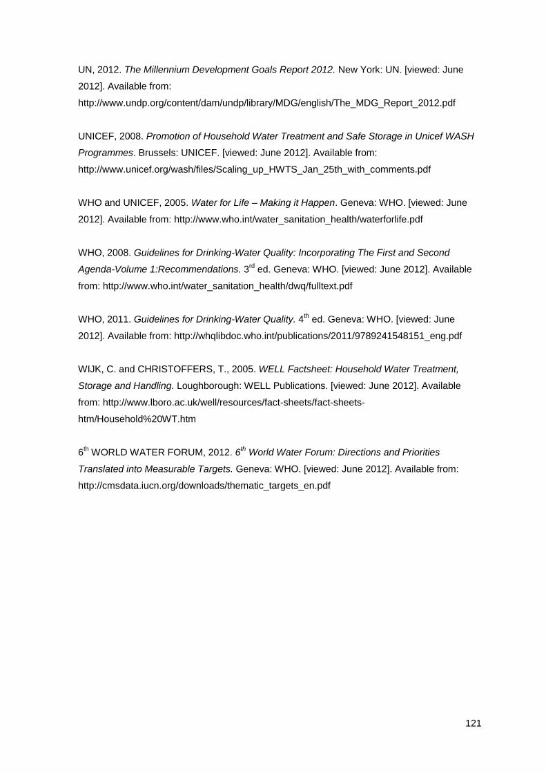
121

UN, 2012. The Millennium Development Goals Report 2012. New York: UN. [viewed: June

2012]. Available from:

http://www.undp.org/content/dam/undp/library/MDG/english/The_MDG_Report_2012.pdf

UNICEF, 2008. Promotion of Household Water Treatment and Safe Storage in Unicef WASH

Programmes. Brussels: UNICEF. [viewed: June 2012]. Available from:

http://www.unicef.org/wash/files/Scaling_up_HWTS_Jan_25th_with_comments.pdf

WHO and UNICEF, 2005. Water for Life – Making it Happen. Geneva: WHO. [viewed: June

2012]. Available from: http://www.who.int/water_sanitation_health/waterforlife.pdf

WHO, 2008. Guidelines for Drinking-Water Quality: Incorporating The First and Second

Agenda-Volume 1:Recommendations. 3rd

ed. Geneva: WHO. [viewed: June 2012]. Available

from: http://www.who.int/water_sanitation_health/dwq/fulltext.pdf

WHO, 2011. Guidelines for Drinking-Water Quality. 4th ed. Geneva: WHO. [viewed: June

2012]. Available from: http://whqlibdoc.who.int/publications/2011/9789241548151_eng.pdf

WIJK, C. and CHRISTOFFERS, T., 2005. WELL Factsheet: Household Water Treatment,

Storage and Handling. Loughborough: WELL Publications. [viewed: June 2012]. Available

from: http://www.lboro.ac.uk/well/resources/fact-sheets/fact-sheets-

htm/Household%20WT.htm

6th WORLD WATER FORUM, 2012. 6

th World Water Forum: Directions and Priorities

Translated into Measurable Targets. Geneva: WHO. [viewed: June 2012]. Available from:

http://cmsdata.iucn.org/downloads/thematic_targets_en.pdf

122

8.0 Appendices

8.1 Experiment A raw data excel sheets

8.1.1 Trial 1

1 2 3 4 average 0 1 2 3 0 1 2 3 0 1 2 3 0 1 2 3 0 1 2 3 0 1 2 3

colour (Hazen) 93 92 74 74 83 83 38 35 34 83 44 50 29 83 55 28 33 83 54 29 39 83 54 25 20 83 54 24 16

pH () 6,9 7,0 7,1 7,1 7 7 7,5 7,6 7,3 7 7,5 7,5 7,5 7 7,4 7,5 7,6 7 7,5 7,5 7,7 7 7,5 7,5 7,7 7 7,6 7,5 7,7

conductivity (μS/cm) 670 680 670 670 673 673 680 670 680 673 690 650 680 673 680 670 680 673 680 620 680 673 690 670 660 673 690 640 660

TDS (ppm) 340 330 330 320 330 330 340 330 340 330 340 330 330 330 340 320 330 330 340 320 340 330 340 330 330 330 340 330 320

temperature (oC) 17,1 17,1 17,2 17,1 17 17 24,8 25,1 24,9 17 24,3 24,6 24,6 17 24,3 25,0 24,6 17 24,1 24,2 24,4 17 24,0 24,5 24,6 17,1 24,0 24,3 24,5

turbidity (NTU) 16 19,8 14,8 14,8 16 16 5,59 3,35 3,03 16 6,78 4,17 2,68 16 5,68 3,35 2,48 16 6,02 3,74 2,60 16 5,38 3,23 3,14 16 5,19 3,28 2,05

sus. solids (transferred) (mg/l) 10 14 8 18 13 13 2 1 5 13 3 4 1 13 3 1 6 13 2 2 2 13 1 2 2 13 1 2 2

dis. oxygen (before) (mg/l) 8,2 8,5 8,5 8,3 8 6,9 6,6 5,9 6,8 6,8 6,0 6,9 6,8 6,3 6,8 6,5 6,1 8 7,1 6,3 5,1 8 7,1 5,9 6,3

dis. oxygen (after) (mg/l) 6,9 7,3 6,5 5,9 6,8 7,3 7,4 6,0 6,9 7,4 6,8 6,3 6,8 7,4 6,7 6,1

E-coli (transferred) (cfu/100ml) 3533 3440 3300 3360 3408 3408 1013 220 113 3408 1093 273 120 3408 1053 240 120 3408 933 227 153 3408 1227 227 60 3408 1253 167 27

volume (left) (ml) 700 500 850 650 850 550 900 650

volume (transfered) (ml) 9300 8800 9150 8500 9150 8600 9100 8450

flowrate (ml/sec) 41,7 39,5 41,0 38,1 366 344 364 338

air temperature (oC) 22,9 24,3 24,4 22,3 22,9 24,3 24,4 22,3 22,9 24,3 24,4 22,3 22,9 24,3 24,4 22,3 22,9 24,3 24,4 22,3 22,9 24,3 24,4 22,3

sus. solids (gr/100ml)

clean filter 0,1952 0,1964 0,2012 0,1867 0,1924 0,1965 0,1976 0,2038 0,1941 0,1886 0,1952 0,1894 0,1919 0,1980 0,2005 0,2010 0,1932 0,2034 0,1923 0,1938 0,1922 0,1876

used filter 0,1962 0,1978 0,202 0,1885 0,1926 0,1966 0,1981 0,2041 0,1945 0,1887 0,1955 0,1895 0,1925 0,1982 0,2007 0,2012 0,1933 0,2036 0,1925 0,1939 0,1924 0,1878

E-coli (cfu)

MLSB (a) 191 182 173 153 53 8 8 59 11 2 40 11 5 46 14 6 62 14 2 48 12 1

MLSB (b) 171 184 157 175 50 8 5 45 17 5 65 14 7 45 10 6 59 10 2 73 7 1

MLSB (c) 168 150 165 176 49 17 4 60 13 11 53 11 6 49 10 11 63 10 5 67 6 2

Pouring 1

SIPHONING POURING CONTROL

raw A B A B Siphoning 1

123

8.1.2 Trial 2

1 2 average 0 1 2 3 0 1 2 3 0 1 2 3 0 1 2 3 0 1 2 3 0 1 2 3

colour (Hazen) 55 35 45 45 30 17 20 45 28 21 14 45 22 26 38 45 22 26 22 45 18 16 25 45 13 15 31

pH () 7,3 7,4 7,35 7,35 7,6 7,8 7,4 7,35 7,4 7,7 7,5 7,35 7,5 7,7 7,6 7,35 7,5 7,7 7,6 7,35 7,5 7,7 7,7 7,35 7,6 7,7 7,7

conductivity (μS/cm) 660 660 660 660 630 650 640 660 640 660 640 660 660 660 650 660 650 660 650 660 650 650 650 660 660 650 650

TDS (ppm) 330 330 330 330 330 320 320 330 320 320 320 330 310 310 320 330 320 320 320 330 320 320 320 330 320 310 320

temperature (oC) 17,9 17,6 17,75 17,75 25,4 25,0 23,5 17,75 24,7 24,6 23,2 17,75 24,6 24,6 23,2 17,75 24,3 24,4 23,0 17,75 24,4 24,5 23,2 17,75 24,1 24,4 23,0

turbidity (NTU) 8,12 7,44 7,78 7,78 3,36 2,22 1,34 7,78 2,98 2,16 1,19 7,78 2,63 2,99 2,44 7,78 3,02 2,49 2,10 7,78 2,86 2,11 1,2 7,78 2,46 2,06 1,43

sus. solids (transferred) (mg/l) 5 2 3,5 3,5 3 3 5 3,5 4 5 4 3,5 2 4 5 3,5 3 2 3 3,5 2 2 3 3,5 5 2 1

dis. oxygen (before) (mg/l) 8,4 8,6 8,5 7,3 6,8 7,0 7,2 6,5 6,8 7,7 7,0 6,9 7,3 6,7 6,7 8,5 8,0 6,3 6,4 8,5 7,5 6,4 6,5


E-coli (transferred) (cfu/100ml) 847 913 880 880 340 87 33 880 293 127 40 880 453 140 40 880 413 113 40 880 407 153 33 880 567 187 47


volume (left) (ml) 550 650 550 850 950 900 950 750


flowrate (ml/sec) 42,4 39,5 42,4 38,6 362 326 362 332


clean filter 0,1906 0,2014 0,2059 0,2007 0,1967 0,1883 0,1934 0,1999 0,1973 0,2006 0,1980 0,2020 0,1939 0,2013 0,1934 0,2062 0,2007 0,1898 0,2118 0,2021

used filter 0,1911 0,2016 0,2062 0,201 0,1972 0,1887 0,1939 0,2003 0,1975 0,2010 0,1985 0,2023 0,1941 0,2016 0,1936 0,2064 0,201 0,1903 0,2120 0,2022

E-coli (cfu)

MLSB (a) 58 41 19 4 1 19 7 3 23 6 1 21 5 4 20 7 0 21 10 1

MLSB (b) 30 53 16 3 2 12 7 2 22 10 1 19 5 1 17 8 2 28 8 3

MLSB (c) 39 43 16 6 2 13 5 1 23 5 4 22 7 1 24 8 3 36 10 3

Pouring 2

CONTROLPOURINGSIPHONING

raw A B A B Siphoning 2

124

125

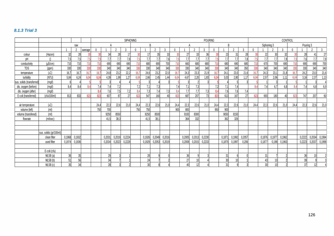
126

8.1.3 Trial 3

1 2 average 0 1 2 3 0 1 2 3 0 1 2 3 0 1 2 3 0 1 2 3 0 1 2 3

colour (Hazen) 32 28 30 30 34 28 17 30 17 35 33 30 27 33 36 30 23 31 28 30 22 30 32 30 28 41 27

pH () 7,5 7,5 7,5 7,5 7,7 7,7 7,8 7,5 7,7 7,7 7,6 7,5 7,7 7,7 7,7 7,5 7,7 7,7 7,8 7,5 7,7 7,7 7,8 7,5 7,6 7,7 7,8

conductivity (μS/cm) 710 710 710 710 690 690 690 710 680 690 700 710 660 680 680 710 680 690 680 710 670 700 690 710 690 690 700

TDS (ppm) 330 330 330 330 340 340 340 330 330 340 340 330 330 340 340 330 340 340 350 330 340 340 340 330 330 340 340

temperature (oC) 16,7 16,7 16,7 16,7 24,8 23,2 22,2 16,7 24,6 23,2 22,0 16,7 24,3 23,3 21,9 16,7 24,1 23,0 21,6 16,7 24,3 23,1 21,8 16,7 24,2 23,0 21,6

turbidity (NTU) 5,84 6,24 6,04 6,04 4,39 1,99 1,27 6,04 2,66 2,45 1,44 6,04 4,67 2,20 1,83 6,04 3,03 2,80 1,17 6,04 2,57 2,06 1,11 6,04 3,16 2,37 1,13

sus. solids (transferred) (mg/l) 6 4 5 5 3 4 4 5 3 4 3 5 3 2 3 5 4 5 3 5 1 3 1 5 1 3 4

dis. oxygen (before) (mg/l) 8,4 8,4 8,4 7,4 7,4 7,2 7,2 7,1 7,3 7,4 7,1 7,3 7,2 7,1 7,4 8,4 7,4 6,7 6,8 8,4 7,4 6,8 6,9


E-coli (transferred) (cfu/100ml) 813 833 823 823 607 87 27 823 547 160 40 823 687 207 73 823 613 167 27 823 693 180 40 823 747 207 60


volume (left) (ml) 750 700 750 750 900 800 950 900


flowrate (ml/sec) 41,5 38,3 41,5 38,1 364 332 362 326


clean filter 0,1968 0,1932 0,2031 0,2019 0,2224 0,1926 0,2049 0,2016 0,2005 0,2013 0,2230 0,1871 0,1992 0,2057 0,1876 0,1977 0,1962 0,2222 0,2034 0,1994

used filter 0,1974 0,1936 0,2034 0,2023 0,2228 0,1929 0,2053 0,2019 0,2008 0,2015 0,2233 0,1875 0,1997 0,206 0,1877 0,198 0,1963 0,2223 0,2037 0,1998

E-coli (cfu)

MLSB (a) 36 35 29 3 1 28 9 0 36 9 3 31 6 0 31 7 2 36 10 2

MLSB (b) 51 56 34 7 1 24 7 2 27 10 4 30 10 1 43 10 2 39 9 3

MLSB (c) 35 34 28 3 2 30 8 4 40 12 4 31 9 3 30 10 2 37 12 4

POURING

Siphoning 3 Pouring 3

CONTROL

raw A B A B

SIPHONING

127

128

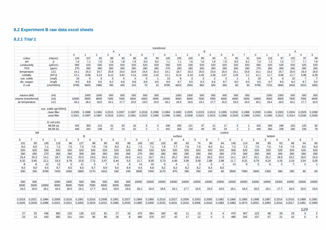
129

0 1 2 3 4 5 6 7 0 1 2 3 4 5 6 7 0 1 2 3 4 5 6 7 0 1 2 3 4 5 6 7

144 116 97 133 97 98 101 95 145 118 96 127 98 90 83 86 145 102 103 80 63 74 56 64 145 114 94 89 63 68 64 65

7,0 7,2 7,5 7,7 7,7 7,8 8,0 8,0 7,1 7,2 7,5 7,5 7,8 7,8 8,0 8,1 7,2 7,1 7,6 7,7 7,8 7,9 8,0 8,1 7,2 7,2 7,5 7,6 7,8 7,9 8,0 8,0

560 520 520 520 520 520 520 520 550 520 520 520 520 520 520 520 550 520 520 520 520 520 520 520 550 520 520 520 520 520 520 520

270 260 260 260 260 260 260 260 270 260 260 260 260 260 260 260 270 260 260 260 260 260 260 260 270 260 260 260 260 260 260 260

14,1 19,3 19,7 20,9 19,4 18,9 19,4 20,3 14,1 18,7 19,3 20,5 19,0 18,4 19,1 19,6 14,1 18,7 19,1 20,2 18,9 18,2 18,5 19,3 14,1 18,7 19,1 20,2 18,9 18,2 18,5 19,3

12,1 11,7 6,89 11,7 6,98 6,28 6,32 5,65 12,1 15,0 6,78 10,8 7,72 5,47 5,44 5,5 11,7 8,05 5,73 4,48 3,59 3,09 2,88 2,98 11,7 8,31 6,79 6,24 4,16 3,19 3,54 3,05

16 9 9 10 7 7 8 8 12 12 5 11 3 7 4 6 14 10 5 4 1 3 5 1 14 9 3 6 2 7 2 1

9,5 8,7 8,5 8,4 8,7 9,0 9,0 9,0 9,5 8,7 8,5 8,5 8,7 8,9 9,0 8,9 9,4 8,8 8,2 8,2 8,2 8,2 8,4 8,5

8780 7210 3940 3430 2310 1600 500 330 8780 7420 4260 2800 2170 1610 530 240 9500 7340 3170 870 280 250 100 60 9500 7090 2600 1350 490 290 80 60

1000 1000 500 500 500 500 500 1000 1000 500 500 500 500 500 10000 10000 10000 10000 10000 10000 10000 10000 10000 10000 10000 10000 10000 10000 10000 10000

10000 9000 8000 7500 7000 6500 6000 5500 10000 9000 8000 7500 7000 6500 6000 5500

18,1 18,4 18,5 19,1 17,7 16,5 19,0 19,0 18,1 18,4 18,5 19,1 17,7 16,5 19,0 19,0 18,1 18,4 18,5 19,1 17,7 16,5 19,0 19,0 18,1 18,4 18,5 19,1 17,7 16,5 19,0 19,0

0,2005 0,1981 0,2003 0,2004 0,2029 0,1998 0,2018 0,2021 0,1984 0,2009 0,2016 0,1991 0,2016 0,2008 0,1991 0,2027 0,1969 0,1990 0,2010 0,2027 0,2009 0,2003 0,2005 0,1982 0,1969 0,1965 0,1998 0,1987 0,2014 0,2010 0,1989 0,1992

0,2021 0,1990 0,2012 0,2014 0,2036 0,2005 0,2026 0,2029 0,1996 0,2021 0,2021 0,2002 0,2019 0,2015 0,1995 0,2033 0,1983 0,2000 0,2015 0,2031 0,2010 0,2006 0,2010 0,1983 0,1983 0,1974 0,2001 0,1993 0,2016 0,2017 0,1991 0,1993

432 356 186 163 125 82 27 20 436 360 215 126 122 81 27 16 470 364 160 45 11 13 5 4 470 367 123 68 28 19 3 2

446 365 208 180 106 78 23 13 442 382 211 154 95 80 26 8 480 370 157 42 17 12 5 2 480 342 137 67 21 10 5 4

control

surface bottomA B

left

8.2 Experiment B raw data excel sheets

8.2.1 Trial 1

0 1 2 3 4 5 6 7 0 1 2 3 4 5 6 7 0 1 2 3 4 5 6 7 0 1 2 3 4 5 6 7

colour (Hazen) 144 107 93 88 65 68 64 59 145 105 100 85 64 71 65 61 144 116 97 133 97 98 101 95 145 118 96 127 98 90 83 86

pH () 7,0 7,1 7,6 7,6 7,8 7,9 8,0 8,0 7,1 7,1 7,6 7,6 7,8 7,9 8,0 8,1 7,0 7,2 7,5 7,7 7,7 7,8 8,0 8,0 7,1 7,2 7,5 7,5 7,8 7,8 8,0 8,1

conductivity (μS/cm) 560 520 530 520 520 520 520 520 550 520 530 520 520 520 520 520 560 520 520 520 520 520 520 520 550 520 520 520 520 520 520 520

TDS (ppm) 270 260 260 260 260 260 260 260 270 260 260 260 260 260 260 260 270 260 260 260 260 260 260 260 270 260 260 260 260 260 260 260

temperature (oC) 14,1 19,3 19,7 20,9 19,4 18,9 19,4 20,3 14,1 18,7 19,3 20,5 19,0 18,4 19,1 19,6 14,1 19,3 19,7 20,9 19,4 18,9 19,4 20,3 14,1 18,7 19,3 20,5 19,0 18,4 19,1 19,6

turbidity (NTU) 12,1 8,66 6,13 6,12 3,62 3,14 3,93 2,24 12,1 8,14 6,19 4,45 3,38 3,07 3,29 3,1 12,1 11,7 6,89 11,7 6,98 6,28 6,32 5,65 12,1 15,0 6,78 10,8 7,72 5,47 5,44 5,5

sus. solids (mg/l) 16 9 3 3 4 4 5 1 12 8 3 3 2 3 1 1 16 9 9 10 7 7 8 8 12 12 5 11 3 7 4 6

dis. oxygen (mg/l) 9,5 8,8 8,5 8,2 8,6 8,8 8,9 8,9 9,5 8,7 8,5 8,3 8,6 8,7 9,0 9,0 9,5 8,7 8,5 8,4 8,7 9,0 9,0 9,0 9,5 8,7 8,5 8,5 8,7 8,9 9,0 8,9

E-coli (cfu/100ml) 8780 6920 2480 780 440 310 70 10 8780 6910 2550 850 500 360 60 30 8780 7210 3940 3430 2310 1600 500 330 8780 7420 4260 2800 2170 1610 530 240

volume (left) (ml) 1000 1000 500 500 500 500 500 1000 1000 500 500 500 500 500 1000 1000 500 500 500 500 500 1000 1000 500 500 500 500 500

volume (transferred) (ml) 10000 9000 8000 7500 7000 6500 6000 5500 10000 9000 8000 7500 7000 6500 6000 5500 10000 9000 8000 7500 7000 6500 6000 5500 10000 9000 8000 7500 7000 6500 6000 5500

air temperature (oC) 18,1 18,4 18,5 19,1 17,7 16,5 19,0 19,0 18,1 18,4 18,5 19,1 17,7 16,5 19,0 19,0 18,1 18,4 18,5 19,1 17,7 16,5 19,0 19,0 18,1 18,4 18,5 19,1 17,7 16,5 19,0 19,0


clean filter 0,2005 0,1988 0,1984 0,2015 0,2007 0,1987 0,2018 0,1998 0,1984 0,1983 0,2005 0,2019 0,2013 0,1995 0,2032 0,1988 0,2005 0,1981 0,2003 0,2004 0,2029 0,1998 0,2018 0,2021 0,1984 0,2009 0,2016 0,1991 0,2016 0,2008 0,1991 0,2027

used filter 0,2021 0,1997 0,1987 0,2018 0,2011 0,1991 0,2023 0,1999 0,1996 0,1991 0,2008 0,2022 0,2015 0,1998 0,2033 0,1989 0,2021 0,1990 0,2012 0,2014 0,2036 0,2005 0,2026 0,2029 0,1996 0,2021 0,2021 0,2002 0,2019 0,2015 0,1995 0,2033

E-coli (cfu)

MLSB (a) 432 350 110 41 20 16 5 0 436 335 121 37 21 17 4 1 432 356 186 163 125 82 27 20 436 360 215 126 122 81 27 16

MLSB (b) 446 342 138 37 24 15 2 1 442 356 134 48 29 19 2 2 446 365 208 180 106 78 23 13 442 382 211 154 95 80 26 8

A B A B

transferred left

130

0 1 2 3 4 5 6 7 0 1 2 3 4 5 6 7 0 1 2 3 4 5 6 7 0 1 2 3 4 5 6 7

143 115 123 155 153 90 105 109 146 139 107 132 103 94 84 114 160 101 94 71 58 73 54 70 160 113 93 92 59 65 74 68

7,1 7,2 7,5 7,5 7,8 7,9 8,0 8,1 7,2 7,2 7,5 7,6 7,8 7,9 8,0 8,1 7,3 7,1 7,6 7,7 7,8 7,9 8,0 8,0 7,3 7,2 7,5 7,6 7,8 7,9 8,0 8,0

550 520 530 520 520 520 520 520 550 520 520 520 520 520 520 520 550 520 530 520 520 520 520 520 550 520 530 520 520 520 520 520

270 260 260 260 260 260 260 260 270 260 260 260 260 260 260 260 270 260 260 260 260 260 260 260 270 260 260 260 260 260 260 260

14,1 19,1 19,4 20,3 18,9 18,2 19,1 19,7 14,1 18,8 19,3 20,1 18,8 18,1 18,6 19,5 14,1 18,6 19,1 20,0 18,7 17,9 18,3 19,1 14,1 18,6 19,1 20,0 18,7 17,9 18,3 19,1

12,4 8,83 10,4 11,0 7,35 5,32 5,99 6,18 11,8 8,83 8,64 11,9 7,84 5,9 4,9 6,31 12,7 8,08 5,67 3,65 3,07 2,83 2,39 3,25 12,7 8,23 5,67 4,43 3,58 3,94 2,45 3,9

17 11 7 12 11 4 7 9 15 12 11 11 8 7 6 8 15 9 5 3 1 2 6 1 15 9 4 4 2 4 5 4

9,5 8,6 8,4 8,4 8,7 9,0 9,2 8,9 9,5 8,6 8,4 8,3 8,8 8,9 9,1 9,0 9,4 8,7 8,3 8,1 8,0 8,3 8,5 8,6

17400 9650 8460 6610 3420 970 710 510 16800 9440 8310 6060 3720 1020 650 610 16800 8850 4600 1510 480 390 170 130 16800 8840 3810 1660 740 560 230 210

1000 1000 500 500 500 500 500 1000 1000 500 500 500 500 500 10000 10000 10000 10000 10000 10000 10000 10000 10000 10000 10000 10000 10000 10000 10000 10000

10000 9000 8000 7500 7000 6500 6000 5500 10000 9000 8000 7500 7000 6500 6000 5500

18,1 18,4 18,5 19,1 17,7 16,5 19,0 19,0 18,1 18,4 18,5 19,1 17,7 16,5 19,0 19,0 18,1 18,4 18,5 19,1 17,7 16,5 19,0 19,0 18,1 18,4 18,5 19,1 17,7 16,5 19,0 19,0

0,1977 0,1961 0,1995 0,2017 0,2019 0,2012 0,1994 0,2013 0,1973 0,1980 0,2001 0,2020 0,2029 0,2001 0,1976 0,1987 0,1988 0,1992 0,2010 0,2006 0,2016 0,1995 0,2023 0,1992 0,1988 0,1978 0,2008 0,2015 0,2028 0,2003 0,2007 0,1986

0,1994 0,1972 0,2002 0,2029 0,2030 0,2016 0,2001 0,2022 0,1988 0,1992 0,2012 0,2031 0,2037 0,2008 0,1982 0,1995 0,2003 0,2001 0,2015 0,2009 0,2017 0,1997 0,2029 0,1993 0,2003 0,1987 0,2012 0,2019 0,2030 0,2007 0,2012 0,1990

870 485 436 302 165 48 34 26 880 484 464 303 187 48 35 30 840 445 239 78 24 19 9 7 840 440 186 83 42 27 9 8

(x) 480 410 359 177 49 37 25 800 460 367 (x) 185 54 30 31 (x) 440 221 73 24 20 8 6 (x) 444 195 83 32 29 14 13

left control

A B surface bottom

8.2.2 Trial 2

0 1 2 3 4 5 6 7 0 1 2 3 4 5 6 7 0 1 2 3 4 5 6 7 0 1 2 3 4 5 6 7

colour (Hazen) 143 105 98 78 67 69 58 65 146 103 96 77 65 73 58 69 143 115 123 155 153 90 105 109 146 139 107 132 103 94 84 114

pH () 7,1 7,1 7,6 7,7 7,8 7,9 8,0 8,1 7,2 7,1 7,6 7,7 7,8 7,9 8,0 8,1 7,1 7,2 7,5 7,5 7,8 7,9 8,0 8,1 7,2 7,2 7,5 7,6 7,8 7,9 8,0 8,1

conductivity (μS/cm) 550 520 530 520 520 520 520 520 550 520 530 520 520 520 520 520 550 520 530 520 520 520 520 520 550 520 520 520 520 520 520 520

TDS (ppm) 270 260 260 260 260 260 260 260 270 260 260 260 260 260 260 260 270 260 260 260 260 260 260 260 270 260 260 260 260 260 260 260

temperature (oC) 14,1 19,1 19,4 20,3 18,9 18,2 19,1 19,7 14,1 18,8 19,3 20,1 18,8 18,1 18,6 19,5 14,1 19,1 19,4 20,3 18,9 18,2 19,1 19,7 14,1 18,8 19,3 20,1 18,8 18,1 18,6 19,5

turbidity (NTU) 12,4 8,08 5,82 4,28 3,77 2,96 3,0 3,11 11,8 7,76 5,7 3,92 3,51 4,09 3,13 3,51 12,4 8,83 10,4 11,0 7,35 5,32 5,99 6,18 11,8 8,83 8,64 11,9 7,84 5,9 4,9 6,31

sus. solids (mg/l) 17 11 4 6 4 3 5 2 15 11 3 4 4 2 3 6,5 17 11 7 12 11 4 7 9 15 12 11 11 8 7 6 8

dis. oxygen (mg/l) 9,5 8,6 8,4 8,4 8,5 8,8 9,0 9,0 9,5 8,6 8,4 8,3 8,7 8,6 9,1 8,8 9,5 8,6 8,4 8,4 8,7 9,0 9,2 8,9 9,5 8,6 8,4 8,3 8,8 8,9 9,1 9,0

E-coli (cfu/100ml) 17400 8750 3430 1110 630 260 140 120 16800 9110 4360 1350 620 290 230 130 17400 9650 8460 6610 3420 970 710 510 16800 9440 8310 6060 3720 1020 650 610

volume (left) (ml) 1000 1000 500 500 500 500 500 1000 1000 500 500 500 500 500 1000 1000 500 500 500 500 500 1000 1000 500 500 500 500 500

volume (transfered) (ml) 10000 9000 8000 7500 7000 6500 6000 5500 10000 9000 8000 7500 7000 6500 6000 5500 10000 9000 8000 7500 7000 6500 6000 5500 10000 9000 8000 7500 7000 6500 6000 5500

air temperature (oC) 18,1 18,4 18,5 19,1 17,7 16,5 19,0 19,0 18,1 18,4 18,5 19,1 17,7 16,5 19,0 19,0 18,1 18,4 18,5 19,1 17,7 16,5 19,0 19,0 18,1 18,4 18,5 19,1 17,7 16,5 19,0 19,0


clean filter 0,1977 0,1978 0,2003 0,2024 0,1989 0,1982 0,2027 0,2011 0,1973 0,1991 0,2000 0,2011 0,1996 0,2012 0,2026 0,20005 0,1977 0,1961 0,1995 0,2017 0,2019 0,2012 0,1994 0,2013 0,1973 0,1980 0,2001 0,2020 0,2029 0,2001 0,1976 0,1987

used filter 0,1994 0,1989 0,2007 0,2030 0,1993 0,1985 0,2032 0,2013 0,1988 0,2002 0,2003 0,2015 0,2000 0,2014 0,2029 0,2007 0,1994 0,1972 0,2002 0,2029 0,2030 0,2016 0,2001 0,2022 0,1988 0,1992 0,2012 0,2031 0,2037 0,2008 0,1982 0,1995

E-coli (cfu)

MLSB (a) 870 425 157 57 31 13 9 8 880 431 219 60 33 14 12 9 870 485 436 302 165 48 34 26 880 484 464 303 187 48 35 30

MLSB (b) (x) 450 186 54 32 13 5 4 800 480 217 75 29 15 11 4 (x) 480 410 359 177 49 37 25 800 460 367 (x) 185 54 30 31

transferred left

A B A B

131

132

133

8.3 Experiment A and B reduction rates tables

8.3.1 Experiment A – Trial 1



0 1 2 3 E. coli RR % 1 E. coli RR % 2 E. coli RR % 3 Average RR% 1 Average RR% 2 Average RR% 3

Siphoning A 3408 1013 220 113 70,27 93,55 96,67

Siphoning B 3408 1093 273 120 67,92 91,98 96,48

Pouring A 3408 1053 240 120 69,10 92,96 96,48

Pouring B 3408 933 227 153 72,62 93,35 95,50

Control Siphoning 3408 1227 227 60 64,01 93,35 98,24

Control Pouring 3408 1253 167 27 63,23 95,11 99,22

96,58

93,15 95,99

94,23 98,73

92,7669,10

70,86

63,62


Siphoning A 880 340 87 33 61,36 90,15 96,21

Siphoning B 880 293 127 40 66,67 85,61 95,45

Pouring A 880 453 140 40 48,48 84,09 95,45

Pouring B 880 413 113 40 53,03 87,12 95,45


Control Pouring 880 567 187 47 35,61 78,79 94,7044,70

87,88

85,61

80,68

95,83

95,45

95,45

64,02

50,76


Siphoning A 823 607 87 27 26,29 89,47 96,76

Siphoning B 823 547 160 40 33,58 80,56 95,14

Pouring A 823 687 207 73 16,57 74,89 91,09

Pouring B 823 613 167 27 25,48 79,75 96,76


Control Pouring 823 747 207 60 9,28 74,89 92,7112,52

85,01

77,32

76,51

95,95

93,93

93,93

29,93

21,02

134

8.3.4 Experiment B – Trial 1

0 1 2 3 4 5 6 7

Transferred A 8780 6920 2480 780 440 310 70 10

Transferred B 8780 6910 2550 850 500 360 60 30

Left A 8780 7210 3940 3430 2310 1600 500 330

Left B 8780 7420 4260 2800 2170 1610 530 240

Control Surface 9500 7340 3170 870 280 250 100 60

Control Bottom 9500 7090 2600 1350 490 290 80 60

E. coli RR % 1 E. coli RR % 2 E. coli RR % 3 E. coli RR % 4 E. coli RR % 5 E. coli RR % 6 E. coli RR % 7

Transferred A 21,18 71,75 91,12 94,99 96,47 99,20 99,89

Transferred B 21,30 70,96 90,32 94,31 95,90 99,32 99,66

Left A 17,88 55,13 60,93 73,69 81,78 94,31 96,24

Left B 15,49 51,48 68,11 75,28 81,66 93,96 97,27

Control Surface 22,74 66,63 90,84 97,05 97,37 98,95 99,37

Control Bottom 25,37 72,63 85,79 94,84 96,95 99,16 99,37

Average RR% 1 Average RR% 2 Average RR% 3 Average RR% 4 Average RR% 5 Average RR% 6 Average RR% 7

Transferred A

Transferred B

Left A

Left B

Control Surface

Control Bottom95,95 97,16 99,05 99,37

94,65 96,18 99,26 99,77

53,30 64,52 74,49 81,72 94,13 96,75

21,24

16,69

24,05

71,36 90,72

69,63 88,32

135

8.3.5 Experiment B – Trial 2

0 1 2 3 4 5 6 7

Transferred A 17400 8750 3430 1110 630 260 140 120

Transferred B 16800 9110 4360 1350 620 290 230 130

Left A 17400 9650 8460 6610 3420 970 710 510

Left B 16800 9440 8310 6060 3720 1020 650 610

Control Surface 16800 8850 4600 1510 480 390 170 130

Control Bottom 16800 8840 3810 1660 740 560 230 210

E. coli RR % 1 E. coli RR % 2 E. coli RR % 3 E. coli RR % 4 E. coli RR % 5 E. coli RR % 6 E. coli RR % 7

Transferred A 49,71 80,29 93,62 96,38 98,51 99,20 99,31

Transferred B 45,77 74,05 91,96 96,31 98,27 98,63 99,23

Left A 44,54 51,38 62,01 80,34 94,43 95,92 97,07

Left B 43,81 50,54 63,93 77,86 93,93 96,13 96,37

Control Surface 47,32 72,62 91,01 97,14 97,68 98,99 99,23

Control Bottom 47,38 77,32 90,12 95,60 96,67 98,63 98,75

Average RR% 1 Average RR% 2 Average RR% 3 Average RR% 4 Average RR% 5 Average RR% 6 Average RR% 7

Transferred A

Transferred B

Left A

Left B

Control Surface

Control Bottom98,81 98,9947,35 74,97 90,57 96,37 97,17

98,91 99,27

44,17 50,96 62,97 79,10 94,18 96,03 96,72

47,74 77,17 92,79 96,34 98,39

136

8.4 Trial sampling prior to experiments

Holywell 1 Holywell 2 Burleigh

colour (Hazen) 75 72 39

pH () 7,0 7,2 7,5

conductivity (μS/cm) 680 690 990

TDS (ppm) 340 340 490

temperature (oC) 16,7 16,7 16,7

turbidity (NTU) 7,14 6,59 2,04

sus. solids (mg/l) 5 4 2

dis. oxygen (mg/l) 8,5 8,6 9,2

E-coli (cfu/100ml) 890 770 580

air temperature (oC) 21 21 21

Holywell 1 Holywell 2 Burleigh


clean filter 0,1904 0,1927 0,2027

used filter 0,1909 0,1931 0,2029

E-coli (cfu)

MFC (a) 30 65 76

MFC (b) 50 75 92

MFC (cfu/100 ml) 800 1400 1680

MLSB (a) 47 45 30

MLSB (b) 42 32 28

MLSB (cfu/100 ml) 890 770 580

pour (sec) siphon (min)

flowrate 30,51 3,45

34,52 3,25

23,49 3,58

21,73 3,24

21,03 3,59

19,21 3,44

average 25,08 3,43

sec 25 223

Documents

Three-Pot Household Water Treatment System: Testing the