Embed Size (px)
Citation preview
ABSTRACT
Title of Thesis: THROUGHPUT EVALUATION AND
OPTIMIZATION IN WIRELESS NETWORKS Nicolas Rentz, Master of Science, 2007 Directed By: Professor John S. Baras
Department of Electrical and Computer Engineering
While wireless communication is progressively replacing wired technology,
methods for the implementation of Wireless Ad-Hoc Networks are currently under
development. As these methods do not require centralized coordination, they are
particularly adapted to environments such as disaster recovery and military
communication and are, therefore, of great interest. Despite the potential advantages,
no reliable methodologies for the design of Wireless Ad-Hoc Networks have been
proposed. This condition is largely due to the complexity of analysis of a wireless
channel in comparison to that of a wired channel. In this thesis, we discuss the
implementation of a tool for wireless network design. Taking a set of nodes and the
corresponding characteristics, this tool computes the routes between each source–
destination pair. The tool then computes the throughput for each connection and,
finally, proposes a method for the optimization of throughput based on probabilistic
routing via sensitivity analysis.

THROUGHPUT EVALUATION AND OPTIMIZATION IN WIRELESS NETWORKS
By
Nicolas Rentz
Thesis submitted to the Faculty of the Graduate School of the University of Maryland, College Park, in partial fulfillment
of the requirements for the degree of Master of Science
2007 Advisory Committee: Professor John S. Baras, Chair/Advisor Professor Richard J. La Professor Adrianos Papamarcou

© Copyright by Nicolas Rentz
2007

Dedication
A Caroline, Gwenaëlle et Marine, A Romain, Doris et Yvonne,
A mes parents, A Jean-Paul
ii

Acknowledgements
I would like to thank my advisor, Professor John S. Baras, for his guidance
and continuous support throughout my graduate studies. I would also like to thank Dr.
Richard J. La and Dr. Adrianos Papamarcou for agreeing to serve on my committee.
Very special thanks to Vahid, George P. and Yadong for their tremendous
help and advice throughout the duration of this work. I would also like to thank Ion,
Ayan and all my friends in the SEIL Lab for the fruitful discussions we had during
these years. Many thanks to Kimberly Edwards for her help in all administrative
matters. To all my friends here and the others abroad, who gave me the chance to
think about something else than my research once in a while: thank you.
I would particularly like to thank Brandy for her continuous help and support
during my studies in the United States. Thanks to her careful proofreading of this
thesis, the document can be read by any normal English speaker.
I also want to thank Dr. Jud Samon and Sue Dougherty for their help and
friendship during the entirety of my stay at the University of Maryland.
Last but not least, I would like to thank my whole family for their amazing
patience and everlasting support. I would not have been able to achieve this work
without them.
I gratefully acknowledge the financial support I received from the Institute for
Systems Research during my graduate studies. This work was partially supported by
the U.S. Army Research Laboratory under the Cooperative Technology Alliance
Program, Cooperative Agreement DAAD19-01-2-0011 and by NASA Marshall
Space Flight Center under award no. NCC8-235.
iii
Table of Contents Dedication ..................................................................................................................... ii Acknowledgements...................................................................................................... iii Table of Contents......................................................................................................... iv List of Tables ............................................................................................................... vi List of Figures ............................................................................................................. vii Chapter 1 : Introduction................................................................................................ 1
1.1 Network design ............................................................................................. 1 1.2 Thesis Organization ...................................................................................... 5
Chapter 2 : Literature review ........................................................................................ 6
2.1 Presentation of 802.11 Physical Layer.......................................................... 6 2.2 Presentation of 802.11 MAC Layer .............................................................. 9 2.3 802.11 Packet Structure .............................................................................. 14 2.4 Performance analysis of 802.11.................................................................. 16
2.4.1 Computation of the saturated throughput in a single cell network ..... 16 2.4.2 Performance modeling of a path in 802.11 multi-hop networks ........ 18
2.5 Optimization in networking ........................................................................ 21 2.5.1 Introduction......................................................................................... 21 2.5.2 Optimization in Congestion Control, Routing and Scheduling .......... 22
Chapter 3 : Neighborhood discovery and Implementation of multi path Routing ..... 25
3.1 Neighborhood discovery............................................................................. 25 3.2 Presentation of the routing algorithm ......................................................... 28 3.3 Lawler’s algorithm for k-Shortest paths with no repeated nodes ............... 28
Chapter 4 : Fixed point modeling ............................................................................... 31
4.1 Introduction................................................................................................. 31 4.2 Methodology............................................................................................... 32 4.3 Presentation of the model.................................................................................. 33
4.3.1 Notation............................................................................................... 33 4.3.2 Scheduler coefficient and serving rate................................................ 34 4.3.3 Computing the transmission failure probability ................................. 35 4.3.4 Computation of the different components of the average time spent in the network.......................................................................................................... 37 4.3.5 Computation of the throughput........................................................... 42 4.3.6 Modus operandi for the computation of the fixed point ..................... 42
4.4 Model Validation: Starvation models ......................................................... 47 4.4.1 Description of 802.11 options adopted in OPNET and the C code .... 47
iv

4.4.2 Flow-in-the-Middle............................................................................. 48 4.4.3 Information Asymmetry...................................................................... 50
4.5 One Connection using one path .................................................................. 52 4.5.1 Preliminary results: Variation of the throughput according to the number of intermediate nodes............................................................................. 52 4.5.2 Evolution of the throughput according to the load for a 5 hops connection ........................................................................................................... 53
4.6 Two Connections using one path each........................................................ 55 4.7 Evolution of the throughput for a network containing three active connections using one path each............................................................................. 57
Chapter 5 : Throughput optimization via Probabilistic Routing................................. 60
5.1 Automatic Differentiation........................................................................... 60 5.1.1 Introduction......................................................................................... 60 5.1.2 The chain rule ..................................................................................... 61
5.2 ADOL-C ..................................................................................................... 64 5.3 Methodology: Gradient Projection ............................................................. 65 5.4 Experimental Results .................................................................................. 68
5.4.1 One connection using multiple paths.................................................. 68 5.4.2 Three connections using multiple paths.............................................. 71
Chapter 6 : Conclusions and Future Work................................................................. 75
6.1 Conclusion .................................................................................................. 75 6.2 Future Work ................................................................................................ 76
Bibliography ............................................................................................................... 78
v

List of Tables Table 6-1: Comparison of the computation time (in seconds) between OPNET and the
fixed point algorithm................................................................................................... 76
vi
List of Figures
Figure 1-1: Structure of the model................................................................................ 4
Figure 2-1: Example of hidden terminals ..................................................................... 9
Figure 2-2: Example of an exposed node scenario ..................................................... 10
Figure 2-3: Example of a communication using RTS/CTS method [13] ................... 12
Figure 2-4: Inter-frame Spacing in 802.11 [14].......................................................... 13
Figure 2-5: Data Frame of an 802.11 packet .............................................................. 14
Figure 2-6: Packet encapsulation ................................................................................ 15
Figure 2-7: Decomposition of an optimization problem [19]..................................... 22
Figure 4-1: Example of a fixed point iteration on the cosine function [24]. .............. 32
Figure 4-2: Architecture of the fixed point algorithm ................................................ 46
Figure 4-3: Flow in the Middle scenario..................................................................... 48
Figure 4-4: Throughput for the different flows in the FIM model ............................. 49
Figure 4-5: Example of Information Asymmetry ....................................................... 50
Figure 4-6: Throughput comparison for Flow 1 and Flow 2 in the Information
Asymmetry example ................................................................................................... 51
Figure 4-7: Throughput’s variation according to the number of intermediate nodes . 53
Figure 4-8: Network Topology 1 ................................................................................ 54
Figure 4-9: Throughput of a connection with a single path vs. traffic load................ 54
Figure 4-10: Network Topology 2 .............................................................................. 55
Figure 4-11: Flow throughput for Topology 2 with an input load of 300 kbps.......... 56
Figure 4-12: Flow throughput for Topology 2 with an input load of 400 kbps.......... 56
vii
Figure 4-13: Network Topology 3 .............................................................................. 58
Figure 4-14: Throughput of 3 connections with single path vs. traffic load............... 59
Figure 5-1: Example of Forward Mode ...................................................................... 62
Figure 5-2: Example of Backward Mode.................................................................... 63
Figure 5-3: Topology 1 with 3 and 5 paths................................................................. 68
Figure 5-4: Network throughput for 1 connection using 1, 3 or 5 paths .................... 69
Figure 5-5: Network throughput for different routing policies according to the number
of available paths, for an input load of 1Mbps ........................................................... 70
Figure 5-6: Network Topology 4 ................................................................................ 71
Figure 5-7: Network Throughput for connection 1 according to the number of
available paths for an input load of 500 kbps ............................................................. 72
Figure 5-8: Network Throughput for connection 2 according to the number of
available paths for an input load of 500 kbps. ............................................................ 72
Figure 5-9: Network Throughput for connection 3 according to the number of
available paths for an input load of 500 kbps. ............................................................ 73
Figure 5-10: Total Network Throughput according to the number of available paths
for an input load of 500 kbps. ..................................................................................... 74
viii
Chapter 1 : Introduction
1.1 Network design
The recent progress in wireless technologies has introduced many new
problems. While most of the communication systems of the past were hierarchical, it
has been shown that the use of wireless ad-hoc networks has many advantages. In
fact, using such configurations reduces the impact of central node bottlenecks in the
network; provides more flexibility as the failure of a node is far less critical than in
hierarchical networks, and offers adaptability to the network architecture over time
(due to either mobility of the nodes, or failures). Wireless ad-hoc networks are
particularly recommended in environments such as disaster recovery and military
communications. On the other hand, this inherent flexibility makes modeling and
prediction of throughput in ad-hoc networks much more difficult. Complexity arises
from attempting to predict the performance of wireless links, as they are dependent on
the activity of other wireless media in the vicinity. The efficiency of wired networks
can be easily predicted as the link capacities are fixed. In wireless networks these
capacities can vary with many factors such as interference caused by neighboring
nodes or transmission power. The dependence of wireless networks on environmental
factors mandates the adoption of a cross-layer approach to the design of wireless
networks. Our model couples the physical, MAC, and routing layers to compute the
optimal throughput of the different connections in a network using probabilistic
routing to achieve optimization. While packet level simulation tools enable the
1

analysis of the physical and medium access control layer, it is often considered too
complex to use such tools. The time taken to run such simulations makes it unrealistic
to apply them to wireless network design. A similar analytical tool would be of use in
emergency situations and military operations as it requires much less time for those
numerical computations than a network simulator. In order to design an efficient
network operating under a given set of constraints, it is necessary to tune multiple
parameters at the physical layer (such as power or modulation scheme) as well as to
tune parameters at the MAC layer (such as number of back-off stages or minimum
contention window size). This tuning can be accomplished by local search algorithms
or, more efficiently, through the use of automatic differentiation in order to achieve
sensitivity analysis. This model would allow the prediction of the performance of a
given network as well as the identification of the nodes that will act as bottlenecks
before implementation.
The approach taken here for implementation of the model is based on the
fixed point method and loss network modeling for performance evaluation, design,
and optimization of wireless or wired networks. Initially used for evaluation of the
blocking probabilities in circuit switched networks [1], loss networks were further
developed for representation and design of complex ATM networks [3]-[5]. More
specifically, Liu et al. [5] presented a way to analyze complicated ATM networks
with elaborated and adaptive routing and multi-service multi-rate traffic by reduced
load approximations.
Baras et al. [2] implemented a model evaluating the packet losses as well as
the throughput in a wireless network. The loss factors of wireless links were
2

considered to be a function of (i) the parameters of the particular link and (ii) the
neighboring link traffic rates. These choices result, in most cases, in the incoming
traffic rate of a link being larger than the outgoing traffic rate. It was shown that, for a
given set of paths for each connection in the network, the network’s throughput can
be approximated by using two sets of equations. The first computes the incoming and
outgoing traffic rate of each link in the network as a function of the loss parameters.
The second calculates the opposite, approximating the loss parameters as a function
of the incoming traffic rates of the link based on Bianchi’s work [15]. By running this
set of equations iteratively on a fixed point, it was possible to compute a solution for
the two parameters and to obtain the throughput for the network.
A continuation of this work includes the incorporation of recent work by
Tobagi et al. [16-17] in which the transmission failure probability of each node and
the different components of the time spent by a packet in each node are approximated
in order to compute the throughput of a single connection in a multi-hop
communication. The fundamental restriction of that work [16-17] is that it does not
allow the computation of the throughput of different flows sharing common nodes.
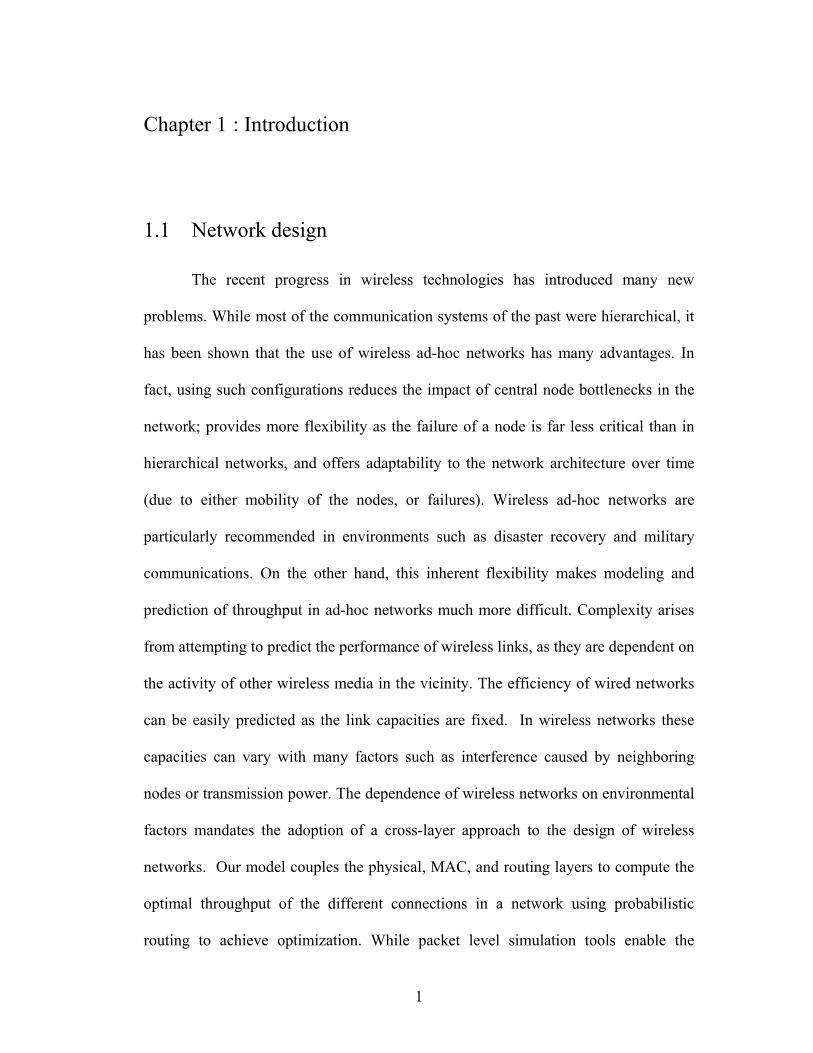
The work presented below and illustrated in Figure 1-1 expands this model to allow
the computation of the throughput of diverse connections using multiple paths, some
of them sharing common nodes, in order to allow for optimization via probabilistic
routing among these proposed paths.
A wireless network is designed through computation of multiple paths for
each connection in order to achieve routing [20]. An iterative fixed point method [3],
[4], [5] is then used with a set of equations computing the traffic rates and losses in
3
the network. A fixed point approach is used to solve the set of equations and to
compute the throughput of each active connection in the network. Using Automatic
Differentiation, the derivatives of the total throughput in the network with respect to
the path routing probabilities are evaluated. Finally, the optimized throughput that can
be achieved in the network is calculated using probabilistic routing with the set of
probabilities we computed based on the optimization algorithm.
Figure 1-1: Structure of the model
4

1.2 Thesis Organization
Chapter 2 of this thesis presents the basics of 802.11 physical layer as well as
the medium access control layer and provides justification of our implementation.
The 802.11 packet structure is described and several papers on wireless network
analysis are discussed to provide the basis for the work described here. Finally,
network design is described as an optimization problem, based on the work by Chiang
et al. [19]. Chapter 3 briefly explains the implementation of neighborhood discovery
and routing in the model. Chapter 4 introduces the employed fixed point algorithm
beginning with an explanation of the basics of the fixed point method followed by a
presentation of the set of equations to be used as well as their implementation.
Finally, the model is validated by setting up experimental networks in OPNET 12.0
and comparing the results between the simulation platform and the new model.
Particular attention is given to capture of the starvation phenomenon in wireless
networks. Chapter 5 exposes the optimization component of the new tool. Automatic
differentiation is presented and the basics of the program adopted for automatic
differentiation are explained [6]. The Gradient Projection method used in the model
for optimization of the throughput based on the path probabilities is introduced. The
chapter concludes with experimental results proving the benefits of optimization in
wireless network design. Chapter 6 summarizes the thesis and describes the future of
this project.
5

Chapter 2 : Literature review
2.1 Presentation of 802.11 Physical Layer
There are several different techniques used to physically transmit packets in
802.11. Each of them allows transmission at different speeds and uses a different
technology. This section describes them to provide justification of the selection of a
single technique for implementation of our simulation platform in OPNET 12.0 [7]
and compares the results with the program developed for this project.
The Frequency Hopping Spread Spectrum (FHSS) [8] scheme uses seventy
nine 1-MHz wide channels in the 2.4GHz frequency band. In order to determine the
order in which this scheme will hop on the selected frequencies, a pseudo-random
number generator is used. This means that the only condition needed for the stations
to be able to communicate with each other is for each of them to use the same seed
for the pseudo-random number generator and that all the stations remain
synchronized in time. The dwell time, which is the amount of time spent in each
frequency band, is a parameter that can be set, but must be less than 400 ms to
prevent FHSS to behave like a narrow-band system. There are several advantages to
the use of FHSS rather than a fixed-frequency transmission:
• Frequency hopping provides a resistance to narrow-band interference, as the
frequency used is constantly changing over time. This provides resistance to
radio interference and is the primary reason for its use in building to building
communications.
6
• FHSS prevents casual eavesdropping due to the need for information on both
the hopping sequence and the dwell time.
• FHSS provides resistance to multi-path fading.
The low bandwidth it provides is a major obstacle to the implementation of
FHSS. This scheme restricts the speed to 1-2 Mbps resulting in a bottleneck for
today’s more rapid communication speeds.
Direct Sequence Spread Spectrum (DSSS) [9] is used in 802.11b, and allows
speeds up to 11 Mbps. DSSS transmission is accomplished through multiplying the
data by a pseudo-random sequence of 1 and -1 values referred to as a “noise signal”
or PN (for Positive Negative) sequence. The result of this multiplexing provides a
signal which appears similar to white noise. The receiver deciphers the message
through multiplying the received signal by the generated noise signal used by the
sender. This is the same as a convolution and deconvolution sequence in
mathematics. Similarly to FHSS, DSSS stations must be synchronized in order for
this scheme to work. An interesting note is the potential for using the frequency at
which the receiver must make synchronizations for determining the relative timing
between sender and receiver. This can in turn be used to compute the position of the
receiving node. Similar methods are used in several satellite navigation systems [9].
DSSS addresses interference as in Code Division Multiple Access (CDMA). Each
station is given a chip sequence to transmit a 1-bit or a 0-bit. This chip sequence is
unique for each station, thus its size in bits will depend on the number of users we
want to be able to handle simultaneously in the system. Each chip sequence is
orthogonal which means that multiplying the chip sequence of station A with the chip
7

sequence of station B will give a result of 0. Every station can send a 1-bit using the
chip sequence it has been assigned and a 0-bit by sending the complement of its chip
sequence. It is assumed that all stations are sending at the same time so that the
resulting signal sent is seen as the linear addition of these 1 or -1 bits sent. For
instance, take 3 stations transmitting simultaneously, A, B and C. If A and B send a 1-
bit and C sends a 0-bit, an output of 1+1-1 = 1 will be observed.
Interference is easily dealt with because of the orthogonality property of these
chip sequences: Take A, B, and C to be the chip sequence of stations A, B, and C
respectively. Then, if A and C send a 1-bit and B sends a 0-bit, the overall signal is
S=(A+B+C) . In order to decipher the signal sent by C, the received signal S is
multiplied by the chip sequence of C (C). Owing to the orthogonality property and
noting S• the normalized inner product of S and C, we get [C 10]:
S•C=(A+B+C)•C=A•C+B•C+C•C=0+0+1=1
The primary advantages of DSSS are:
• Strong resistance to intentional or unintentional jamming, as shown above
• Potential for sharing of a single channel amongst multiple users
• Potential for determining the geographic position of the nodes through the
synchronization scheme.
The main disadvantage of DSSS is its cost which is much higher than that of FHSS.
Orthogonal Frequency Division Multiplexing (OFDM) is used with 802.11a
and 802.11g to achieve higher data rates (up to 54 Mbps). Here, 52 frequencies are
used for data transmission and synchronization purposes. This feature enables OFDM
to be significantly more resistant to narrow-band interference [8]. OFDM is resistant
8
to multi-path fading, provides improved tolerance to time synchronization errors over
DSSS, and provides a high spectral efficiency. OFDM is sensitive to frequency
synchronization problems and the Doppler Effect. In addition, there is a high
implementation cost associated with OFDM [11]. As Bianchi [15], Medepalli [16]
and Hira [17] based their studies on 802.11 networks using CDMA, which is not used
in ODFM, DSSS is selected throughout this work.
2.2 Presentation of 802.11 MAC Layer
Unlike with Ethernet, synchronizing the transmission of wireless stations is a
complex problem. There are several cases in which a wireless transmission offers
very different problems to those of a wired communication.
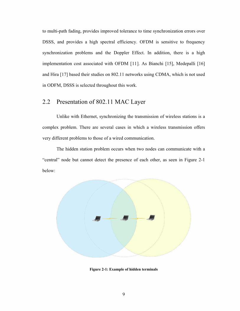
The hidden station problem occurs when two nodes can communicate with a
“central” node but cannot detect the presence of each other, as seen in Figure 2-1
below:
Figure 2-1: Example of hidden terminals
9
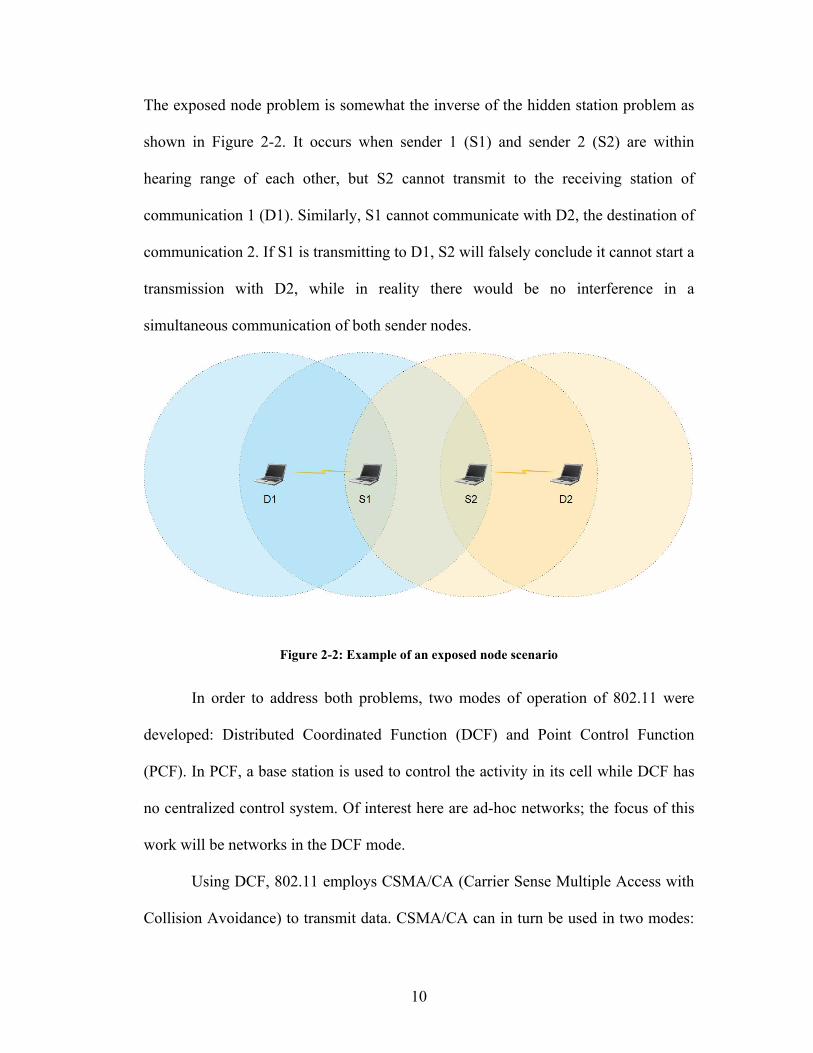
The exposed node problem is somewhat the inverse of the hidden station problem as
shown in Figure 2-2. It occurs when sender 1 (S1) and sender 2 (S2) are within
hearing range of each other, but S2 cannot transmit to the receiving station of
communication 1 (D1). Similarly, S1 cannot communicate with D2, the destination of
communication 2. If S1 is transmitting to D1, S2 will falsely conclude it cannot start a
transmission with D2, while in reality there would be no interference in a
simultaneous communication of both sender nodes.
Figure 2-2: Example of an exposed node scenario
In order to address both problems, two modes of operation of 802.11 were
developed: Distributed Coordinated Function (DCF) and Point Control Function
(PCF). In PCF, a base station is used to control the activity in its cell while DCF has
no centralized control system. Of interest here are ad-hoc networks; the focus of this
work will be networks in the DCF mode.
Using DCF, 802.11 employs CSMA/CA (Carrier Sense Multiple Access with
Collision Avoidance) to transmit data. CSMA/CA can in turn be used in two modes:
10

Basic Access and RTS/CTS (Request-To-Send/Clear-To-Send). Basic Access is a
two-way handshake, in which only a positive acknowledgment is transmitted by the
destination upon reception of a successfully received packet. The primary concern
with basic access is that it does not provide a method for addressing the presence of
hidden terminals as shown in Figure 2-1. In order to accommodate this eventuality,
RTS/CTS was developed. This is a four-way handshake technique in which a node
needing to send data first sends a RTS frame. If the destination node is available at
that time, it sends back a CTS frame to the source node. Any node within hearing
range of the sending and/or receiving node will be able to receive this RTS or CTS
frame respectively. The other nodes will be aware of the future communication
scheduled to take place and will refrain from sending data during the time given both
in the RTS and CTS frame. On the other hand, when such a node can hear the RTS
frame but does not receive the CTS frame associated with it, it does not interfere with
the existing communication and is thus authorized to transmit data. This can be
observed in the case of the exposed node problem depicted in Figure 2-2 above, with
S2 receiving the RTS of S1, but not hearing the CTS of D1. It is important to note the
main assumption for RTS/CTS’s scheme: All nodes are assumed to have identical
transmission/receiving ranges.
Tanenbaum provides an example of RTS/CTS [12]. The problem addresses a
network containing 4 stations. Station A wants to transmit to station B. Station C is
within hearing range of station A (whether B and C are within hearing range of each
other is of no importance in this case). Station D is within hearing range of station B
but cannot hear station A. When A decides to send to B, it sends an RTS to B to ask
11
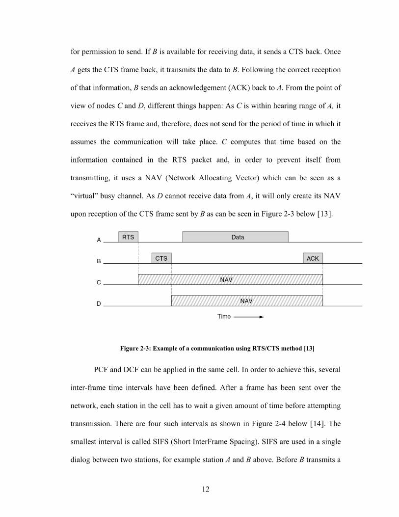
for permission to send. If B is available for receiving data, it sends a CTS back. Once
A gets the CTS frame back, it transmits the data to B. Following the correct reception
of that information, B sends an acknowledgement (ACK) back to A. From the point of
view of nodes C and D, different things happen: As C is within hearing range of A, it
receives the RTS frame and, therefore, does not send for the period of time in which it
assumes the communication will take place. C computes that time based on the
information contained in the RTS packet and, in order to prevent itself from
transmitting, it uses a NAV (Network Allocating Vector) which can be seen as a
“virtual” busy channel. As D cannot receive data from A, it will only create its NAV
upon reception of the CTS frame sent by B as can be seen in Figure 2-3 below [13].
Figure 2-3: Example of a communication using RTS/CTS method [13]
PCF and DCF can be applied in the same cell. In order to achieve this, several
inter-frame time intervals have been defined. After a frame has been sent over the
network, each station in the cell has to wait a given amount of time before attempting
transmission. There are four such intervals as shown in Figure 2-4 below [14]. The
smallest interval is called SIFS (Short InterFrame Spacing). SIFS are used in a single
dialog between two stations, for example station A and B above. Before B transmits a
12
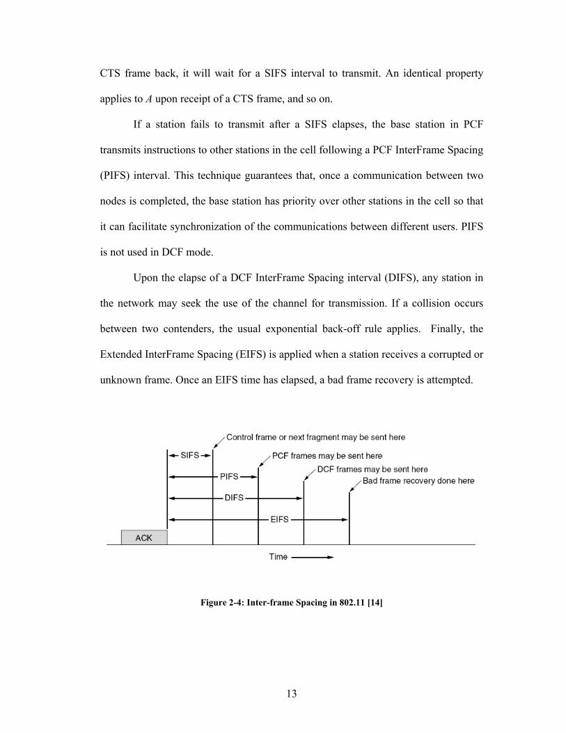
CTS frame back, it will wait for a SIFS interval to transmit. An identical property
applies to A upon receipt of a CTS frame, and so on.
If a station fails to transmit after a SIFS elapses, the base station in PCF
transmits instructions to other stations in the cell following a PCF InterFrame Spacing
(PIFS) interval. This technique guarantees that, once a communication between two
nodes is completed, the base station has priority over other stations in the cell so that
it can facilitate synchronization of the communications between different users. PIFS
is not used in DCF mode.
Upon the elapse of a DCF InterFrame Spacing interval (DIFS), any station in
the network may seek the use of the channel for transmission. If a collision occurs
between two contenders, the usual exponential back-off rule applies. Finally, the
Extended InterFrame Spacing (EIFS) is applied when a station receives a corrupted or
unknown frame. Once an EIFS time has elapsed, a bad frame recovery is attempted.
Figure 2-4: Inter-frame Spacing in 802.11 [14]
13
2.3 802.11 Packet Structure
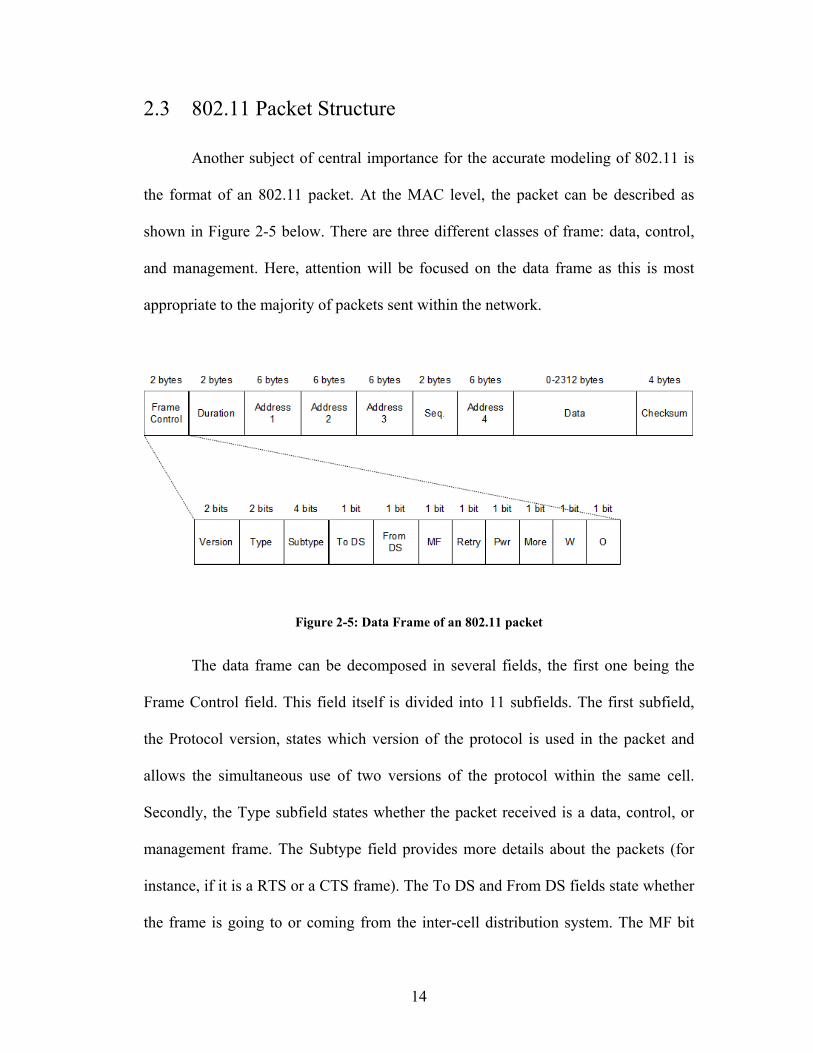
Another subject of central importance for the accurate modeling of 802.11 is
the format of an 802.11 packet. At the MAC level, the packet can be described as
shown in Figure 2-5 below. There are three different classes of frame: data, control,
and management. Here, attention will be focused on the data frame as this is most
appropriate to the majority of packets sent within the network.
Figure 2-5: Data Frame of an 802.11 packet
The data frame can be decomposed in several fields, the first one being the
Frame Control field. This field itself is divided into 11 subfields. The first subfield,
the Protocol version, states which version of the protocol is used in the packet and
allows the simultaneous use of two versions of the protocol within the same cell.
Secondly, the Type subfield states whether the packet received is a data, control, or
management frame. The Subtype field provides more details about the packets (for
instance, if it is a RTS or a CTS frame). The To DS and From DS fields state whether
the frame is going to or coming from the inter-cell distribution system. The MF bit
14

indicates that more fragments are to be expected. The Retry bit specifies whether or
not the frame is a retransmission. The Power management bit is only used in PCF and
enables the base station to ask another wireless node to shift to or from sleep state.
The More bit signifies that the sender has additional frames to transmit to the
receiver, while the W bit indicates the encryption of the packet using WEP. The O bit
tells the receiver of the packet that every frame in that sequence having the O bit set
to 1 must absolutely be treated in order. The second field of the data frame, the
Duration field, indicates how long this frame and the associated acknowledgement
will occupy the channel. This field, also present in the control frames, is the field used
by neighboring stations to compute their NAV. There are also four addresses in the
MAC header. While two of them are reserved for the source and destination of the
packet, the other two are used for the source and destination base station in case of
inter-cell traffic. The Sequence field permits the numbering of fragments, while the
Data field contains the payload of the frame, followed by a checksum in the
Checksum field.
Overall, a packet is organized as illustrated in Figure 2-6. Here, the IP header
and the TCP header have been added to more clearly show the encapsulation of the
packet.
Figure 2-6: Packet encapsulation
15

2.4 Performance analysis of 802.11
2.4.1 Computation of the saturated throughput in a single cell
network
Bianchi et al. [15] first exposed a new way of analyzing the overall saturation
throughput in a single cell wireless network for both the basic access method and the
RTS/CTS mechanism. While most previous work depended primarily on simulations
or limited analytical models to study the performance of 802.11, Bianchi’s method
takes into account the details of the back-off protocol using Markov chain analysis.
The approximation in the model is the assumption that the collision probability of a
packet transmitted by either station in the network is constant and independent of
other collisions and of the number of previous retransmissions of that packet. The
primary factor evaluated throughout this work is the saturation throughput. It is
known that 802.11 shows some instability upon saturation. For instance, if we
increase the offered load in a given network over time, the network throughput will
rise and maintain the ideal load up to a threshold value after which it will begin to
decrease, eventually converging asymptotically to a value lower than the maximum
throughput of the network. This throughput value is defined by Bianchi as the
saturation throughput [15]. Assuming a single cell network (meaning there are no
hidden nodes) and ideal channel condition (i.e. the channel losses are null and every
node has the same data rate) this model takes a network with a fixed, given number of
saturated stations. In other words, each station in the network has a packet to send at
each time step. The analytical model is then broken down in two different steps. First,
16

the probability τ for a single station to transmit a packet in a random slot time is
computed via a Markov model. It is of importance to notice that τ is independent of
the DCF mechanism used (either basic access or RTS/CTS). Second, the possible
events in a random time slot are carefully studied in order to compute the saturation
throughput in both the RTS/CTS mode and Basic Access as a function of the
previously estimated τ. The probability that a station transmits in a randomly chosen
slot time is given by [15]:
2(1 2 )(1 2 )( 1) (1 (2 ) )m
pp W pW p
τ −=
− + + −
where m represents maximum number of back-off stages, p is the conditional
collision probability and W is the minimum congestion window, . In other
words, . This result is applied by Tobagi et al. [
minCW
min max2m CW CW= 16-17] and will be
of use in the analytical model presented in Chapter 4. Finally, note that Bianchi [15]
defines the throughput as a ratio of the expected value of the payload information sent
in a slot time to the expected duration of a slot time:
[payload information sent in a slot time][length of a slot time]
EThroughputE
=
This means, in that case, that the throughput is measured in bits/s. Here the
representation of the throughput is similar to that used by Tobagi et al., however, the
definition used in this thesis will be slightly different in that it will represent a
percentage: the ratio of the expected value of the amount of data received by the
destination node to the expected value of the amount of data injected in the network
by the source node.
17
2.4.2 Performance modeling of a path in 802.11 multi-hop
networks
Tobagi and Medepalli propose a study of wireless networks allowing the
computation of several properties of an 802.11 network such as throughput, delay,
and fairness [16]. They demonstrate that the exponential back-off is not as useful as
intended to prevent flow starvation problems. In fact, a careful choice of the
minimum contention window provides better control of these problems. Here, the
intention is to compute the throughput of a flow in a non-saturated regime using a set
of probabilities correlated with each other by a set of fixed point equations. The
shortcoming of Bianchi’s work [15] occurs as a result of the assumption that there are
no hidden nodes within the network. Networks containing hidden nodes are quite
common and display properties different from those of single cell networks. The
notion of synchronization between the different stations in the network is lost and it
can no longer be assumed that all nodes will sense a busy channel and stop/resume
their back-off counter simultaneously when a transmission starts/ends. Every node
will have a different perception of the channel according to its position relative to the
other nodes in the network. Another assumption of Bianchi’s work [15] that has been
removed from the work of Tobagi et al. is the non-emptiness of the queue of each
node in the network. The probability that a node has a packet in its queue and wishes
to use the channel is included in their model [16]. This probabilistic design is based
on two observations. Consider node S to be the source of the communication and
node D to be the destination. If node S senses the channel to be idle, there is a single
possibility for node D to sense it busy. This occurs if node D physically or virtually
18

(through a NAV) senses node J transmitting at that instant while S cannot because it
is out of range of the communication taking place between J and another node. Note
that this case is symmetric between D and S. The second observation concerns the
case in which D experiences a collision. There are two possibilities: either at least one
node within hearing range of both D and S transmits in the same back-off slot as S or
at least one node within hearing range of D but hidden from S transmits during the
vulnerable period (the vulnerable period is defined to be the period during which the
neighbors of D are not aware of the transmission between S and D and may cause a
collision by transmitting). It is interesting to remark that this model considers only the
set of nodes having some activity in the network (i.e. either sending traffic or
receiving traffic) and can, therefore, easily deal with nodes transmitting at different
frequencies. Nodes transmitting in a frequency f2 will not be included in the set of
nodes transmitting in f1 and will have no influence on the computation of the fixed
point for these nodes. The methodology of this work is to first compute the collision
probabilities in the network and, secondly, to compute the expected transmission time
for the two-node communication. The methodology is expanded to compute the
collision probability for each node in the path considered [17]. The average
transmission time of each node in the path is then estimated. It is shown that this
model exhibits very good performance in identifying starvation problems and
bottlenecks in the network [16]. Tobagi et al. expanded that work [17] by computing
the throughput of a path in a wireless communication. As opposed to previous work
in the area [18], this model takes into account the fact that some links in the path of
interest may not be saturated, even if the source of the link is. This model can be
19

extended to compute the throughput of multiple paths along the network under the
restraining condition than no two paths can share a common node. In other words,
this model takes into account inter-path interferences when more than one connection
is active in the network. Under the assumption that each source of a connection is
saturated, this paper computes the throughput along each path by computing the
average service time for a packet at each intermediate node i, E[Ti]. Once this value
has been computed for each node, the node having the highest service time is used
(i.e. the bottleneck in the path), bn, and the throughput is computed with the
following equation, where P represents the packet size:
[ ]bn
PThroughputE T
=
The work presented here expands the model of Tobagi et al. in order to be
able to compute the throughput of different flows. Here, several paths can have one or
more nodes in common. These nodes can either be the source and destination for the
computation of the throughput of a connection using multiple paths or the same
intermediate nodes if two different connections are going through the same node in
their respective path(s).
20
2.5 Optimization in networking
2.5.1 Introduction
Optimization tools are widely used in engineering applications. When
designing a new component, it is critical to ensure that it will be used its maximum
capacity. Networking is not an exception to this rule. Whether the discussion is of
wired, wireless, or even space networks, the question is always an optimization
problem. Wang et al. [19] expose the methods for characterization of a network
design problem as an optimization problem and the techniques for dividing it into
different “sub problems” to provide tools for competitive design, i.e. a design that
gives satisfactory performance from the components of interest.
The most famous networking model is the layered OSI reference model. This
model consists of decomposing the major tasks of networking in different layers in
order to achieve competitive and reliable communication. Each layer can be seen as a
separate optimization problem with various constraints and different variables to
optimize depending on the task allocated to that layer. At this point, the interfaces
between the OSI layers can be interpreted as functions of the different optimization
variables of each layer. This allows for coordination of the different optimization sub
problems in order to provide a satisfactory overall solution, i.e. a solution that
consists of a trade-off between the different layers to obtain the best compromise and
achieve an overall optimal reference model. An example of this decomposition can be
seen in Figure 2-7 below.
21
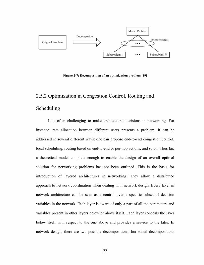
Figure 2-7: Decomposition of an optimization problem [19]
2.5.2 Optimization in Congestion Control, Routing and
Scheduling
It is often challenging to make architectural decisions in networking. For
instance, rate allocation between different users presents a problem. It can be
addressed in several different ways: one can propose end-to-end congestion control,
local scheduling, routing based on end-to-end or per-hop actions, and so on. Thus far,
a theoretical model complete enough to enable the design of an overall optimal
solution for networking problems has not been outlined. This is the basis for
introduction of layered architectures in networking. They allow a distributed
approach to network coordination when dealing with network design. Every layer in
network architecture can be seen as a control over a specific subset of decision
variables in the network. Each layer is aware of only a part of all the parameters and
variables present in other layers below or above itself. Each layer conceals the layer
below itself with respect to the one above and provides a service to the later. In
network design, there are two possible decompositions: horizontal decompositions
22
and vertical decompositions. Horizontal decomposition consists of taking one
functionality module and processing it using different computing units, possibly
geographically distant; this is the concept of distributed computing. Vertical
decomposition deals with applying a Network Utility Maximization (NUM) over
different layers of the network. Each of these decompositions can be seen as a
different layer of the subnet and the Lagrangian functions, or their duals can be
interpreted as being the interfaces between two consecutive layers.
As an example, let us present a case-study [19]. The equilibrium of TCP-
AQM (Active Queue Management) is considered. Assume that TCP-AQM is stable,
performs faster than the time needed for routing updates and that only single-path
connections are considered. The equilibrium can be presented as the solution of a
NUM and its dual, which is clearly an optimization problem.
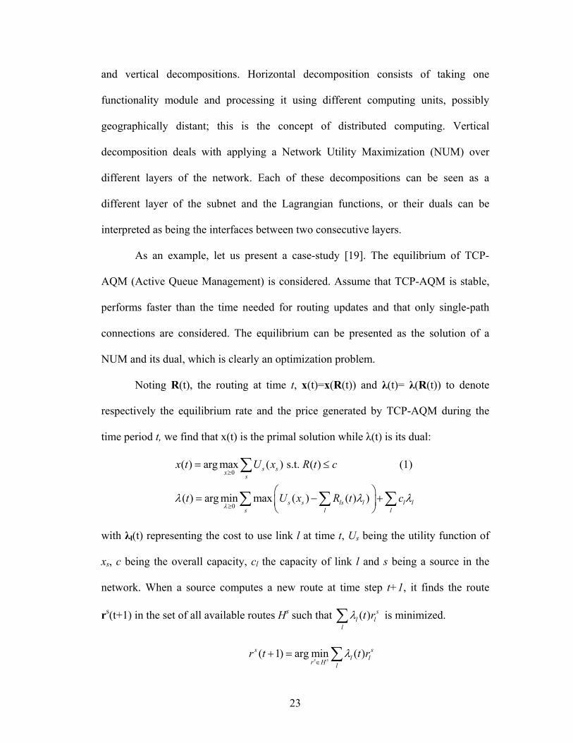
Noting R(t), the routing at time t, x(t)=x(R(t)) and λ(t)= λ(R(t)) to denote
respectively the equilibrium rate and the price generated by TCP-AQM during the
time period t, we find that x(t) is the primal solution while λ(t) is its dual:
0
0
( ) arg max ( ) s.t. ( ) (1)
( ) arg min max ( ) ( ) )
s sx s
s s ls ls l
x t U x R t c
t U x R tλ l l
lcλ λ λ
≥
≥
= ≤
⎛ ⎞= −⎜ ⎟
⎝ ⎠+
∑
∑ ∑ ∑
with λl(t) representing the cost to use link l at time t, Us being the utility function of
xs, c being the overall capacity, cl the capacity of link l and s being a source in the
network. When a source computes a new route at time step t+1, it finds the route
rs(t+1) in the set of all available routes Hs such that ( ) sl l
lt rλ∑ is minimized.
( 1) arg min ( )s s
s sl l
r H lr t t rλ
∈+ = ∑
23
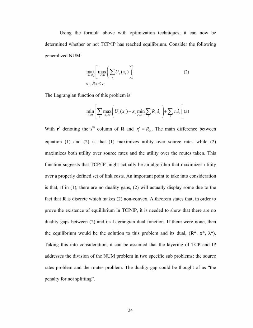
Using the formula above with optimization techniques, it can now be
determined whether or not TCP/IP has reached equilibrium. Consider the following
generalized NUM:
0(2)max max ( )
s.t
ns sR R x s
U x
Rx c
∈ ≥
⎡ ⎤⎛ ⎞⎢ ⎥⎜ ⎟
⎝ ⎠⎣ ⎦≤
∑
The Lagrangian function of this problem is:
0 0(3)min max ( ) min
s ss
s s s ls l l lx rs lU x x R c
λλ λ
≥ ≥ ∈Η
⎡ ⎤⎛ ⎞− +⎢ ⎥⎜ ⎟
⎝ ⎠⎣ ⎦∑ ∑
l∑
ls
With rs denoting the sth column of R and slr R= . The main difference between
equation (1) and (2) is that (1) maximizes utility over source rates while (2)
maximizes both utility over source rates and the utility over the routes taken. This
function suggests that TCP/IP might actually be an algorithm that maximizes utility
over a properly defined set of link costs. An important point to take into consideration
is that, if in (1), there are no duality gaps, (2) will actually display some due to the
fact that R is discrete which makes (2) non-convex. A theorem states that, in order to
prove the existence of equilibrium in TCP/IP, it is needed to show that there are no
duality gaps between (2) and its Lagrangian dual function. If there were none, then
the equilibrium would be the solution to this problem and its dual, (R*, x*, λ*).
Taking this into consideration, it can be assumed that the layering of TCP and IP
addresses the division of the NUM problem in two specific sub problems: the source
rates problem and the routes problem. The duality gap could be thought of as “the
penalty for not splitting”.
24

Chapter 3 : Neighborhood discovery and Implementation of
multi path Routing
3.1 Neighborhood discovery
The very first operation executed by the program is neighborhood discovery.
The program is given an input file used for computing the available routes between
two nodes, the throughput for each connection, and finally the optimal throughput.
The content of the file is the following:
First, it states which time instant is described and how many nodes are in the
network at that time. Then, a description of each node is given containing the
following information:
• Identity of the node. Identifies the node in the program.
• Position of the node. Given in the Cartesian referential.
• Power. Represents the transmitting power of this node.
• Г, the noise threshold for that node.
• NumConn displays the number of connections for which this node will be the
source. If NumConn is non nil, then following this field is a description of
each of these connections in the following way:
Destination: ToS: Data rate: Numpaths
Here, Destination represents which node will be the destination for this
connection while ToS is the type of service demanded for this connection (i.e.
video, data, or voice) and Data Rate the amount of bandwidth demanded by
25
the source for this connection. Finally, Numpaths is the number of paths
desired to carry on this connection. If enough paths between the source and
destination are available, then the desired number of paths is going to be used
to carry data in the connection, otherwise the maximum number of paths
found between the source and the destination is used.
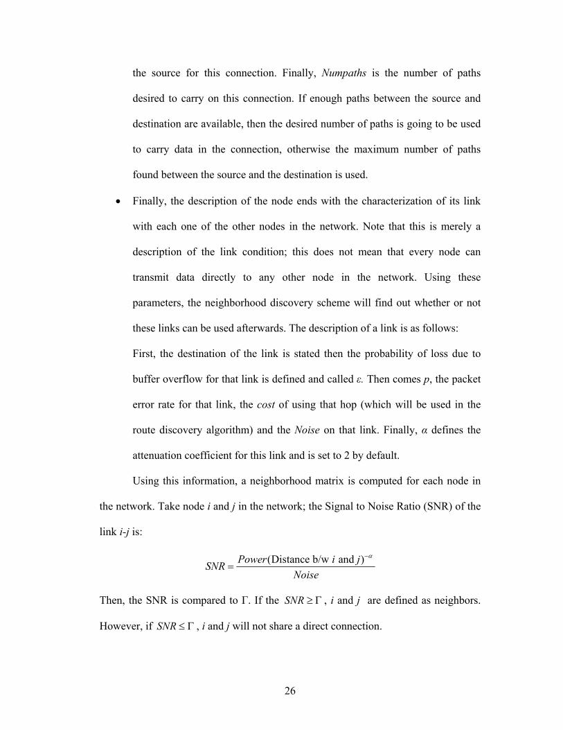
• Finally, the description of the node ends with the characterization of its link
with each one of the other nodes in the network. Note that this is merely a
description of the link condition; this does not mean that every node can
transmit data directly to any other node in the network. Using these
parameters, the neighborhood discovery scheme will find out whether or not
these links can be used afterwards. The description of a link is as follows:
First, the destination of the link is stated then the probability of loss due to
buffer overflow for that link is defined and called ε. Then comes p, the packet
error rate for that link, the cost of using that hop (which will be used in the
route discovery algorithm) and the Noise on that link. Finally, α defines the
attenuation coefficient for this link and is set to 2 by default.
Using this information, a neighborhood matrix is computed for each node in
the network. Take node i and j in the network; the Signal to Noise Ratio (SNR) of the
link i-j is:
(Distance b/w and )Power i jSNRNoise
α−
=
Then, the SNR is compared to Г. If the SN , i and j are defined as neighbors.
However, if , i and j will not share a direct connection.
R ≥ Γ
SNR ≤ Γ
26

At that point, the program reads a matrix of links between all the nodes of the
network. Each link is assigned a weight of one which can later be changed to other
weights based on the distance, bandwidth, interference, or other performance related
criteria. Since the routing algorithm outputs the K-shortest paths having the lowest
overall cost using this parameter, the paths fitting best specific requirements can be
selected later on. The routing program is called for each source-destination pair which
allows the number of paths desired for each pair individually to be set. The program
then outputs the paths found, the cost associated with each one of them, and the
number of paths found (as in some cases, there might not be as many loop free paths
as the user requested). The main advantage of using the Dreyfus algorithm in this
project is that, in many cases, the optimal path might not be the one which contains
the least number of intermediate hops for instance. Moreover, the ultimate goal is to
create a probability distribution which will define the proportion in which the traffic
should be sent over the set of paths computed by the routing algorithm.
Ultimately, once the paths needed for each of the source-destination pairs
defined in the network have been found, the probabilities are initialized in order to
use the computed paths for each pair to a uniform distribution. Then, the optimization
algorithm is launched which will maximize the throughput of the network using
automatic differentiation to optimize the routing probabilities associated with each
connection existing in the network at each time slot. Note that a source node might
have more than one connection (with different throughputs) to a given destination.
Running the optimization scheme on total network throughput ensures that the
27
probability distribution found by this scheme is going to optimize the overall network
performance.
3.2 Presentation of the routing algorithm
Routing is implemented using Lawler’s adaptation of the Dreyfus algorithm.
The particularity of Dreyfus algorithm is that it computes more than the shortest path
between a source and a destination. This algorithm allows the user to compute the K-
shortest paths to a given source-destination pair. The advantage of this scheme is that
it is particularly adapted to the needs of this project, in which several paths can be
used for each connection and in which a specific set of constraints must be satisfied
for each path used. There are mainly two versions of the Dreyfus algorithm: the first
one computes the K-shortest paths of a source-destination pair and can return paths
containing the same node (including the source node) multiple times. The second
version does not allow loops in the paths it computes. Though computationally harder
(the length of computation is on the order of O(K.n3), where K represents the number
of paths computed, and n is the total number of nodes in the network), the second
scheme was implemented as only loop free paths are relevant in the design of ad-hoc
wireless networks.
3.3 Lawler’s algorithm for k-Shortest paths with no repeated
nodes
In this section, the algorithm used to compute K loop-free shortest paths is
presented step-by-step based on the work of Lawler [20]. Here, 1 defines the source
28

node and d the destination node. The arcs here are the existing connections between
the nodes and their neighbors, i.e. if node a and node b are within hearing range of
each other then there exists an arc between them. Note that in this model, the
transmitting power and the noise threshold of each node in the network can be set,
thus it is possible in some cases to have directive arcs (for instance, if a can transmit
to b but b cannot transmit to a due to a lower transmission power). However, in all
the networks tested, the assumption that identical nodes were used in the network was
taken, so there will not be any directive arc in this work.
1. Provided all arc lengths are superior or equal to zero, compute the shortest
path from 1 to d using Dijkstra’s algorithm. Add this path to the list of paths,
LIST, and set k=1.
2. If LIST is empty, then stop the algorithm: This means there are no more paths
to be found between 1 and d. If LIST is non empty, then output the shortest
path in the list and label it Pk. If k=K, exit, as the desired number of paths
have been computed. Otherwise, go to step 3.
3. Assume in this step that Pk contains arcs (1, 2), (2,3), …, (q-1, q), (q, d).
Suppose as well that Pk is the shortest available path between 1 and d amongst
all the paths forced to include arcs (1, 2), (2,3), …, (p-1, p), where p q≤ and
some edges of p are excluded from the set of candidate edges (this condition is
stored in LIST alongside the entry Pk as will be seen below).
a. If p q= , apply Dijkstra’s algorithm to find the shortest path between 1
and d with the following conditions:
i. Arcs (1, 2), (2,3), …, (p-1, p) are included in the path.
29

ii. Arc (p, d) can not be used in this path, in addition to the edges
of p that are excluded as stated above.
If such a path can be computed, put it in LIST, along with the
description of the conditions with which it was computed (which edges
were excluded, etc.)
b) If p q> , apply Dijkstra’s method to compute the shortest path
between 1 and d as well, but with this set of conditions instead:
i) Arcs (1, 2), (2,3), …, (p-1, p) are included in the path, but
arc (p, p+1) is excluded, alongside with the set of excluded
paths stored next to the entry Pk in LIST.
ii) Arcs (1, 2), (2,3), …, (p, p+1) are included in the path, but
arc (p+1, p+2) is excluded.
iii) …
q-p-2) Arcs (1, 2), (2,3), …, (q-2, q-1) are included in the path, but
arc (q-1, q) is excluded.
q-p-1) Arcs (1, 2), (2,3), …, (q-1, q) are included in the path, but
arc (q, d) is excluded.
Dispose each shortest path found by following one of the conditions
stated above in LIST, along with a description of the condition
followed to find this path. Set 1k k= + and go back to step 2.
30
Chapter 4 : Fixed point modeling
4.1 Introduction
In his first analysis of IEEE 802.11 [15], the analytical model Bianchi
proposed computed the saturated throughput of a wireless network and assumed to
have ideal channel conditions and a finite number of users. It also made the
assumption of a single cell network (i.e. every node in the network is within hearing
range of every other node in the network). While these estimations trigger very
accurate results in most cases, it has the problem that it does not illustrate starvation
problems in which some connections consume the bandwidth of others due to their
respective geographical locations. An example of this is the “Flow in the Middle”
case where a source can hear the activity of two other sources that cannot sense each
other. This results in very low throughput for the first source and almost 100%
throughput for the other two sources. In the work by Medepalli [16], Wang [21] and
Garetto [22], analyses have been carried out in order to compute the throughput of
individual nodes (as opposed to Bianchi’s total network throughput computation) in
networks containing hidden nodes. Finally Tobagi and al. extended their model to
compute the throughput of individual nodes belonging to multi-hop connections [17].
This model allows computing the throughput for multiple paths as long as these paths
do not share a common node. In the model presented in this thesis, that work is
extended to enable the computation of throughput for multiple paths having one or
several common nodes.
31
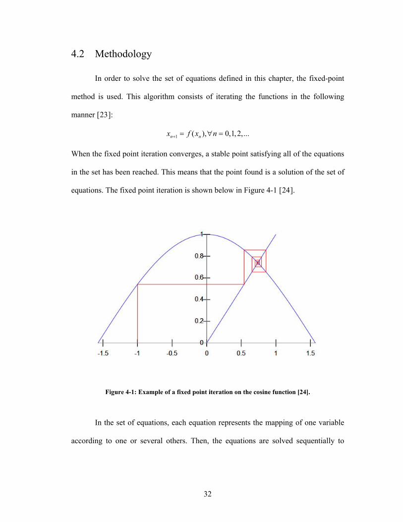
4.2 Methodology
In order to solve the set of equations defined in this chapter, the fixed-point
method is used. This algorithm consists of iterating the functions in the following
manner [23]:
1 ( ), 0,1,2,...n nx f x n+ = ∀ =
When the fixed point iteration converges, a stable point satisfying all of the equations
in the set has been reached. This means that the point found is a solution of the set of
equations. The fixed point iteration is shown below in Figure 4-1 [24].
Figure 4-1: Example of a fixed point iteration on the cosine function [24].
In the set of equations, each equation represents the mapping of one variable
according to one or several others. Then, the equations are solved sequentially to
32
apply all the mappings and insure convergence to a fixed point satisfying all
equations in the set.
4.3 Presentation of the model
4.3.1 Notation
The model considered consists of N nodes and P paths. Notice that the number
of paths in the model is the addition of all the paths used by each source-destination
pair of the network. In this model, the unit of time used is the length of a time slot in
IEEE 802.11, which is 50μs. The following notation is used throughout this chapter:
• Pi represents the set of paths containing node i (either as the source,
destination, or a simple intermediary node).
• Ci is the set of transmitting neighbors of node i.
• Ci+ refers to the set Ci plus node i itself.
• Ci- refers to the set outside carrier sense range of node i. Thus, if Ω denotes
the set containing all transmitting nodes in the network, . i iC C− +∪ = Ω
• hi,p denotes the node coming after node i in path p.
• li,j characterizes the physical layer transmission failure between node i and
node j. As of now, li,j’s have to be given to the program as an input parameter.
To retrieve these values, a network similar to the network evaluated by the
analytical model is set up on a network simulator platform (OPNET 12.0 [7]).
Using the results obtained by OPNET, the Bit Error Rate (BER) of each
connection of interest in the network is retrieved. Using this information, the
packet error rate li,j is computed using the following formula:
33
( ), ,1 (1 ) packet size bits
i j i jl BER= − −
Take Ti,p to be the service time measured between the selection of a packet for
transmission along path p by the node i scheduler and the arrival of this packet at its
destination.
4.3.2 Scheduler coefficient and serving rate
The average number of packets that are served at source node i and will go
through path p in a time slot is denoted by ki,p and is given by the following
relationship:
, , ', '
', , '
,,
,
, ', '
' , '
if [ ] 11 1
1otherwise
[ ]1
i
i
i p i pi pm m
p Pi p i p
i pi p m
i p
i pi pm
p P i p
E T
k
E T
λ λβ β
λβ
λβ
∈
∈
⎧≤⎪ − −⎪
⎪⎪= ⎨−⎪
⎪⎪
−⎪⎩
∑
∑
Where λi,p denotes the arrival rate of packets at node i going through path p:
,
, ,
, , ,
(in packets/slots) if is a source node
(1 ) for every other nodei p
i p conn p
mh p i p i p
P input rate i
k
λ
λ β
= ⋅
= −
and βi,p is the probability of transmission failure in either the physical or MAC layer.
Here, m represents the maximum number of retries (set to 6 throughout these
experiments), and Pconn,p characterizes the probability of using path p in connection
conn. The formula is justified by the fact that a packet will have to be transmitted on
average ,1/(1 )mi pβ− times, at a rate of λi,p. There exist two different situations when
scheduling packets: Either the utilization of node i is less than 1 and all incoming
packets can be served (as is described in the first line of the computation of ki,p) or the
34
scheduler coefficients have to be normalized by the utilization of the node as can be
seen in the second line of the equation.
When the scheduler coefficients are obtained, the fraction of time that a node i
is serving a packet going through a path p can be computed:
, , ,[ ]i p i p i pk E Tρ =
4.3.3 Computing the transmission failure probability
To obtain the transmission failure probability, the probability ",i pα of a node
accessing the channel, assuming that this node is scheduled to serve a packet on the
path p, needs to be characterized. Note W and M to be respectively the minimum and
maximum window size. Here, W = 16 and M = 1024 in order to fit 802.11
specifications. Then L, the number of back-off stages can be computed as
2log MLW
= , and the following formula for ",i pα is obtained [16]:
,",
, , ,
2(1 2 )(1 2 ) ( 1)(1 (2 ) )
i pi p L
i p i p i pW Wβ
αβ β β
−=
− + + −
Using this result, the probability that a node j in the neighborhood of a
transmitting node i expects a transmission of this node through a path p, , ,i p jα , can be
computed. This can happen if i has scheduled a transmission on path p and no
neighbors of node i hidden from j are actually transmitting. Noting ,i jθ the probability
that a neighbor of node i hidden from node j is transmitting:
35
", , , , ,
", , , ,
, ,
(1 )
0 otherwise
i p j i p i j i p i
i p i i p i p
i p j
j Cα ρ θ α
α ρ α
α
= − ∀ ∈
=
=
To compute ,i jθ , the average time spent transmitting in the path p for a node i,
, needs to be determined. There are two possibilities when node i is transmitting:
it is either carrying a successful transmission or spending time in a failed
transmission. Define and
,i pv
,i pd ,i pf as the time spent in successful transmission and
failed transmission, respectively. Then, is the average transmission time, which is
the time spent in successful transmission times the probability that no retransmission
is needed plus the average time spent in failed transmission (
,i pv
,i pf ) times the
probability that we had to retransmit the packets, namely:
,2 3, , , , ,
,
1...
1
mi pm
i p i p i p i p i pi p
ββ β β β β
β−
+ + + + =−
. Thus,
,, , , ,
,
1(1 )
1
mi pm
i p i p i p i p i pi p
v dβ
β ββ
−= − +
− ,f
Details on the computation of and ,i pd ,i pf will be given in the next subsection.
This enables the computation of ,i jθ :
, ', ,
' , '
1 1[ ]
n pi j n p
p Pn n pn C Ci j
vE T
θ ρ− ∈∈ ∩
⎛ ⎞= − −⎜ ⎟⎜ ⎟
⎝ ⎠∑∏ '
Now, the transmission failure probability ,i pβ can be characterized. The probability
for a transmission originating from node i and going through path p to be successful
is given by the probability that there is no link failure, no neighbors hi,p hidden from i
are transmitting, no new transmission of neighbors of hi,p (including hi,p itself) that are
36
neighbors of i as well will occur, and finally the probability that no transmission of
neighbors of hi,p hidden from i, and hi,p itself will occur during the vulnerable period
Vi,p (period during which these neighbors are not aware of the transmission between i
and hi,p and might cause a collision by transmitting themselves). This gives:
,
, , , ,
, ,
, , , , ', , ',' '
1 (1 )(1 ) (1 ) (1 ) i p
i p i p i p i pj ji ih hi p i p
V
i p i h h i j p h j p hp P p Pj C C j C C
lβ θ α+ + −∈ ∈∈ ∩ ∈ ∩
= − − − − − α∑ ∑∏ ∏
, ( , )i p RTSV T i p SIFS= +
4.3.4 Computation of the different components of the average
time spent in the network
Finally, the different times spent in the network need to be computed to obtain
the throughput of each active connection in the network. Ti,p is the total time spent by
a packet scheduled to go trough path p after it was scheduled for transmission at node
i. This total time spent can be divided in five components:
1. di,p: Time consumed in successful transmission by node i for packets sent in
path p.
2. fi,p: Time consumed in failed transmission by node i for packets sent in path p.
3. bi,p: Average back-off time of node i for a packet going through path p.
4. ui,p: Average time consumed by successful transmission of neighbors of node i
during Ti,p.
5. ci,p: Average time consumed in failed transmission during Ti,p.
37
The average service time is:
, , , , , ,[ ] (1 )mi p i p i p i p i p i pE T d u b cβ= − + + +
and here, denoting TRTS(i,p), TCTS(i,p), TP(i,p), and TACK(i,p) to be respectively the
time taken to transmit a RTS, CTS, data, or acknowledgment packet between node i
and the next node in the path p, hi,p:
, ,( , ) ( , ) ( , ) ( , )i p RTS CTS i p P ACK i pd T i p SIFS T h p SIFS T i p SIFS T h p= + + + + + + ,
The time spent in failed transmission, ,i pf , is characterized by the average time
spent in packet transmission failure plus the average time consumed by failures due to
RTS/CTS. Define ,i pε to be the probability of transmission at the physical layer when
packets and acknowledgments are being sent in the network (called stage 2 of 802.11
transmission, stage 1 being the moment where RTS/CTS frames are sent in the
network):
, ,,
, ,
(1 )i p i pi p P H
i p i p
fε ε
τ τβ β
= + −
,
( , )
( , ) ( , ) ( , )
H RTS
P RTS CTS i p P
T i p SIFS
T i p SIFS T h p SIFS T i p SIFS
τ
τ
= +
= + + + + +
where Hτ is the time taken by the transmission of an RTS frame, and Pτ represents
the time spent for the transmission of a packet.
The average time spent in back-off stages is
, ,0 2
mnn
i p i pn
CWb β=
= ∑
Where CWn/2 is the average back-off time at the nth retransmission trial and m is the
maximum number of retrial attempts.
38
The computation of ui,p, the average time taken by successful transmission of
neighbors of node i, is somewhat more involved. Several other probabilities need to
be computed beforehand. First, the probability of successful transmission by node i
when it is scheduled to transmit a packet through path p, qi,p, is given by:
", , ,(1 )i p i p i pq α β= −
Now, assuming the events of unsuccessful transmission of neighbors of node i are
independent, the probability of having a successful transmission in the neighborhood
of a node i can be written as:
, , , ' , ''
1 (1 ) 1 (1 )ji
i p i p j p j p j ip Pj C
r q q ρ θ∈∈
⎛ ⎞⎛ ⎞= − − − −⎜ ⎟⎜ ⎟⎜ ⎟⎝ ⎠⎝ ⎠
∑∏ ,
The probability that the next successful transmission will come from node i, knowing
that there is a successful transmission originating from the neighborhood of i, can be
expressed as:
,,
,
i pi p
i p
qr
γ =
Calling Qi,p the number of successful transmissions by neighbors of i during the time
Ti,p:
,,
,
1[ ] i p
i pi p
E Qγ
γ−
=
Now, the time taken by each successful transmission by neighbors of node i
needs to be computed to get ui,p. Define tk,i as the time taken by the kth successful
transmission of node i neighbors. To compute tk,i, the probability gi,j,p that a successful
transmission in the neighborhood of i belongs to a neighbor j, given that this
successful transmission is not carried out by i itself, needs to be characterized:
39
, ' , ' ,'
, ,, ,
(1 )j
j p j p j ip P
j i pi p i p
qg
r q
ρ θ∈
−=
−
∑
Now, calling dj the average time taken by a successful transmission by node j, for all
the paths using j:
, ' , ' , ''
, ' , ''
(1 )
(1 )j
j
mj p j p j p
p P
j mj p j p
p P
k dd
k
β
β∈
∈
−=
−
∑∑
And:
, , , ,[ ]i
k i p j i p jj C
E t g∈
= d∑
Finally, assuming the time taken by the kth transmission of a neighbor of i is
independent of the number of successful transmission in the neighborhood of i:
, ,[ ] [i p i p k i pu E Q E t , , ]=
To conclude, ci,p, the average time spent in unsuccessful transmission due to
collision at a node i while transmitting using path p needs to be expressed.
The computation of ci,p is somewhat similar to the evaluation of ui,p. Firstly, the
average number of failed transmissions for node i while sending packets using the
path p will be computed. Secondly, the time spent in each failed transmission will be
expressed.
The average number of failed transmissions due to collisions during the time
Ti,p is the ratio of the probability of having a successful transmission by node i, given
that at least one transmission has taken place in its neighborhood (called xi,p), and the
probability that a failure will happen in the neighborhood of i, given that at least one
transmission has happened in this neighborhood (yi,p).
40
Since the probability that at least one transmission has taken place in the
neighborhood of i is given by : " ", , , ' , '
'
1 (1 ) 1 (1 )i j
i p i j j p j pj C p P
α θ ρ∈ ∈
⎛ ⎞⎛ ⎞− − − −⎜ ⎟⎜ ⎟⎜ ⎟⎝ ⎠⎝ ⎠
∏ ∑ α
,,
" ", , , '
'
1 (1 ) 1 (1 )ji
i pi p
i p j i j p j pp Pj C
qx
α θ ρ∈∈
=⎛ ⎞⎛ ⎞
− − − −⎜ ⎟⎜ ⎟⎜ ⎟⎝ ⎠⎝ ⎠∑∏ , 'α
and
,,
" ", , , '
'
11 (1 ) 1 (1 )
ji
i pi p
i p j i j p j pp Pj C
ry
α θ ρ∈∈
= −⎛ ⎞⎛ ⎞
− − − −⎜ ⎟⎜ ⎟⎜ ⎟⎝ ⎠⎝ ⎠∑∏ , 'α
Now, the average time spent in a failed transmission for a node i given that it is
scheduled to serve path p, wi,p, is given by :
", ' , ' , ' , , '
'
,
", ' , ' , ' ,
'
(1 )
(1 )
ji
ji
j p j p j p j i j pp Pj C
i p
j p j p j p j ip Pj C
fw
α β ρ θ
α β ρ θ
+
+
∈∈
∈∈
⎛ ⎞−⎜ ⎟
⎝ ⎠=⎛ ⎞
−⎜ ⎟⎝ ⎠
∑ ∑
∑ ∑
And finally, the average time spent in failed transmission for node i when it is
scheduled to serve path p is given by:
,, ,
,
i pi p i p
i p
yc w
x=
41

4.3.5 Computation of the throughput
Lastly, the throughput in the network needs to be expressed. The throughput
for each active connection in the network is computed as follows: For each
connection, the ratio of the sum of the arrival rates of each path used in that
connection to the input rate given at each path p used in the given connection is
computed. Note that as the probabilistic weighting given to each path in this part of
the computation is uniform, the input rate of each path is going to be exactly the
same. However, when optimizations are performed on the throughput of each
connection, the probability distribution will change as will the input rate of each path.
Define Thc to be the throughput of a connection c having i as the source node.
Then:
,
,
c
c
last pp P
cfirst p
p P
Thλ
λ∈
∈
=∑∑
where first and last denote the source and destination nodes in connection c,
respectively, and Pc designates the set of paths p used to carry out the communication
demanded for the connection c.
4.3.6 Modus operandi for the computation of the fixed point
In order to insure better chances of convergence for the fixed point algorithm,
several choices have been made during design:
• Initialization: The values of the parameters are initialized assuming the
communication is perfect for every connection, i.e.: the input rate of the
connection is propagated throughout every path of the connection. This means
42
that assuming perfect communication, there will be no congestion in
intermediary nodes in the path. The time Ti,p is assumed to consist only of the
time taken by successful transmission plus the back-off time needed for the
first trial (it is assumed no retransmission is needed). Namely,
, , ,
00, , ,
0, ,
[ ] for
[ ]2
[ ]2
i p i p i p
i p i p i p
i p i p
E T d b m
CWE T d
CWE T d
β
0= + =
= +
= +
Moreover, as the transmission conditions are considered perfect, every probability
of failure is set to zero which means:
", , , , , ,
, , ,
0
0,i p i p i p i p i p i p
i p j i j
f u c r
j
β α
α θ
= = = = = =
= = ∀
Because of this assumption, the other parameters are set as follows:
vi,p, the average transmission time of node i for a transmission on path p contains
only the average transmission time taken for successful transmissions, and
,i p i pk ,λ= since node i can serve all incoming packets:
, ,i p i pv d=
and
, , ,[ ]i p i p i pE Tρ λ=
• Fixed point iteration model: Here, an iteration is defined to be the
computation of all parameters of each node contained in each path of each
active connection in the network. After an iteration, all parameters in the
network have been updated. To insure symmetry in the computations in the
43

model, it is necessary to make sure all computations are consistent. That
means for each iteration, the new values of each hop in each path of each
connection are computed using the values computed in the previous iteration,
instead of updating the values as they are computed. This prevents
dissymmetry in the computations. For instance, if the computed values were
updated as an iteration progresses, the values of the parameters of the source
node of a path would be updated and used to compute the new parameters of
the second node in the path, and so on. That would mean the information
available when the parameters of each node are computed as the nodes of a
path and the paths of each connection are subsequently explored, will not be
the same for each node: the computation of the parameters of the first node of
the first path studied will be based on parameters that will be completely out
of date when the last node of the last path considered is reached. By making
sure the final values computed after the last iteration in the fixed point are
used, this inequality is corrected.
• Use of memory in the fixed point: To insure convergence of the fixed point,
the concept of memory needs to be introduced when updating the results in
the algorithm. This guarantees that there will be no oscillation between two
values when the fixed point is iterated. To introduce memory, the following
method is adopted: in order to compute the new value of the parameter, two
results are used. First, the value of the parameter that was saved in the
previous iteration, which will be called old and, second, the value outputted
44

by the result of the equation computing the new parameter, called
new_equation. The new value is then defined as follows:
+ (1- ) _ , 0 1new value old new equationη η η= ≤ ≤
where η here allows some control over the importance given to the old value
when computing the new one.
• Convergence condition: The fixed point is only exited when the expectation
of the service time, E[Ti,p], converges for all nodes in all paths considered
during the same iteration. Note that the same node can have different values of
E[Ti,p] as a given node might be involved in communications taking place in
different paths. A convergence happens if and only if all the expectation times
of all nodes involved in an active connection in the network have converged.
The expectation of the service time is selected to be the variable through
which to control the convergence of our fixed point as this variable depends
on all the other parameters in the set of equations.
To summarize, the architecture of the fixed point algorithm is given in Figure 4-2
below:
45
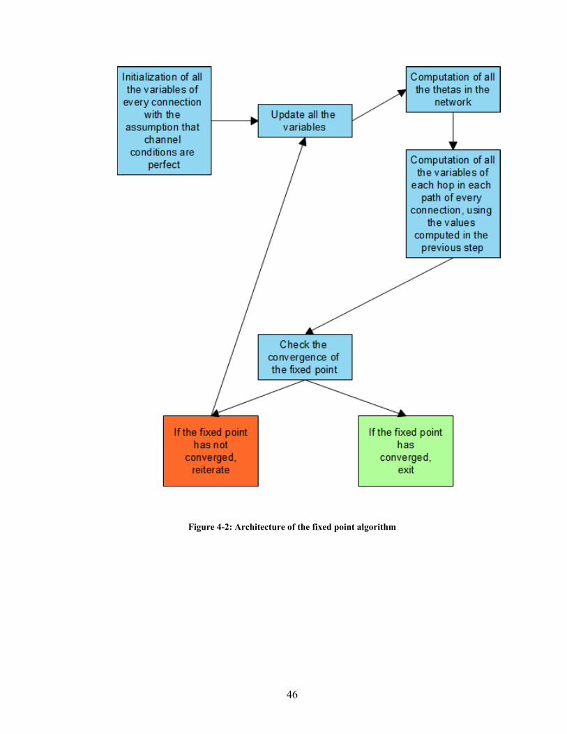
Figure 4-2: Architecture of the fixed point algorithm
46

4.4 Model Validation: Starvation models
4.4.1 Description of 802.11 options adopted in OPNET and the
C code
In order to validate the fixed point model, different specific architectures are
set in OPNET 12.0 [7] and their results are compared to the results obtained with the
C program. A number of parameters in OPNET should be adjusted in order to provide
comparable results between OPNET and the C code (which will be referred to as
WND in this work) from networks with identical settings.
Simulation durations are 20 minutes to guarantee that the behavior of wireless
communication is recorded for normal use. The packet payload size in OPNET is set
to 1024 bytes. Due to the MAC, IP, and TCP/UDP header along with the size of the
checksum, the total size of packet is 1124 bytes. To adapt the simulations with the
program, the packet size is set to constant. The traffic is set to send at a constant data
rate which will vary according to the experiments made. RTS/CTS mode is used for
communication between the wireless nodes while the capacity of the wireless channel
is set to 1Mbps. Direct-Sequence Spread Spectrum (DSSS) modulation technique is
adopted at the physical layer as it is the most widely installed in mobile wireless
nodes currently. Finally, the transport protocol used is UDP as the input rate needs to
be fixed in OPNET models to parallel the C program. TCP will automatically adjust
its rate in case of packet drop, therefore, it would not be adapted for such a
comparison.
47
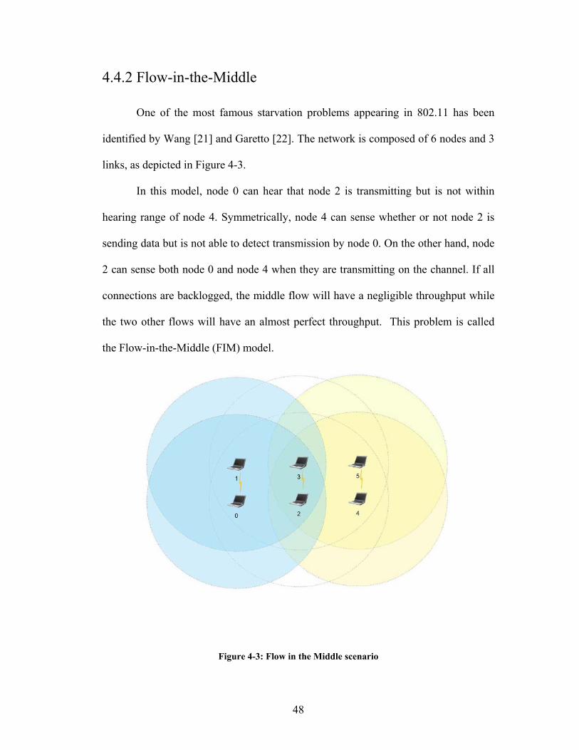
4.4.2 Flow-in-the-Middle
One of the most famous starvation problems appearing in 802.11 has been
identified by Wang [21] and Garetto [22]. The network is composed of 6 nodes and 3
links, as depicted in Figure 4-3.
In this model, node 0 can hear that node 2 is transmitting but is not within
hearing range of node 4. Symmetrically, node 4 can sense whether or not node 2 is
sending data but is not able to detect transmission by node 0. On the other hand, node
2 can sense both node 0 and node 4 when they are transmitting on the channel. If all
connections are backlogged, the middle flow will have a negligible throughput while
the two other flows will have an almost perfect throughput. This problem is called
the Flow-in-the-Middle (FIM) model.
Figure 4-3: Flow in the Middle scenario
48
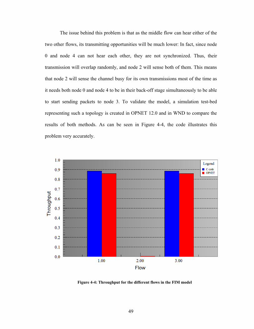
The issue behind this problem is that as the middle flow can hear either of the
two other flows, its transmitting opportunities will be much lower: In fact, since node
0 and node 4 can not hear each other, they are not synchronized. Thus, their
transmission will overlap randomly, and node 2 will sense both of them. This means
that node 2 will sense the channel busy for its own transmissions most of the time as
it needs both node 0 and node 4 to be in their back-off stage simultaneously to be able
to start sending packets to node 3. To validate the model, a simulation test-bed
representing such a topology is created in OPNET 12.0 and in WND to compare the
results of both methods. As can be seen in Figure 4-4, the code illustrates this
problem very accurately.
Figure 4-4: Throughput for the different flows in the FIM model
49
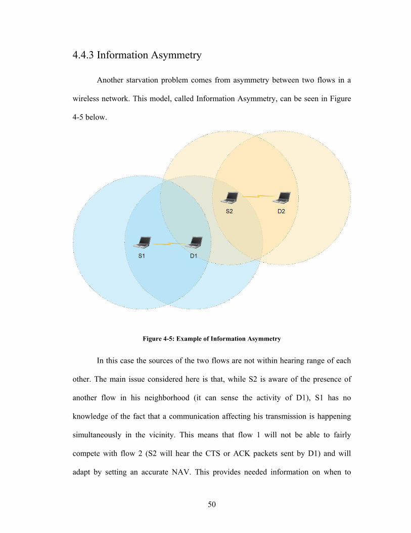
4.4.3 Information Asymmetry
Another starvation problem comes from asymmetry between two flows in a
wireless network. This model, called Information Asymmetry, can be seen in Figure
4-5 below.
Figure 4-5: Example of Information Asymmetry
In this case the sources of the two flows are not within hearing range of each
other. The main issue considered here is that, while S2 is aware of the presence of
another flow in his neighborhood (it can sense the activity of D1), S1 has no
knowledge of the fact that a communication affecting his transmission is happening
simultaneously in the vicinity. This means that flow 1 will not be able to fairly
compete with flow 2 (S2 will hear the CTS or ACK packets sent by D1) and will
adapt by setting an accurate NAV. This provides needed information on when to
50
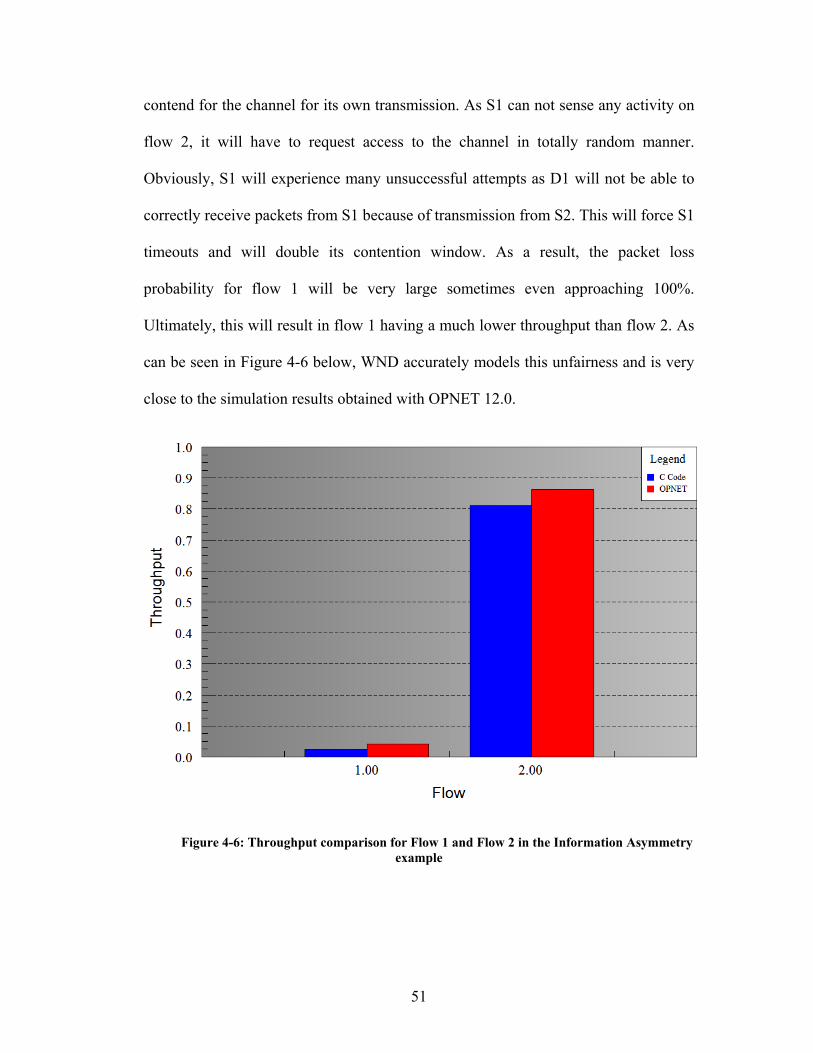
contend for the channel for its own transmission. As S1 can not sense any activity on
flow 2, it will have to request access to the channel in totally random manner.
Obviously, S1 will experience many unsuccessful attempts as D1 will not be able to
correctly receive packets from S1 because of transmission from S2. This will force S1
timeouts and will double its contention window. As a result, the packet loss
probability for flow 1 will be very large sometimes even approaching 100%.
Ultimately, this will result in flow 1 having a much lower throughput than flow 2. As
can be seen in Figure 4-6 below, WND accurately models this unfairness and is very
close to the simulation results obtained with OPNET 12.0.
Figure 4-6: Throughput comparison for Flow 1 and Flow 2 in the Information Asymmetry example
51

4.5 One Connection using one path
4.5.1 Preliminary results: Variation of the throughput according
to the number of intermediate nodes
In order to test further the validity of the model, a simple network is set up. In
the first setting, the source node and the destination node are the only two nodes in
the network. Then, an intermediate node (in line with these two nodes) is inserted to
serve as a hop between the source and the destination and the throughput is obtained.
Then one more intermediate node is added in each new measurement until there are 3
intermediate nodes in the network. This creates a connection of 5 hops in total. In
theory, the results should be as follows:
For a network of two nodes, a perfect throughput should be obtained as there are no
other transmitting nodes and the destination can be reached directly by the source.
When the connection contains three nodes, the maximum achievable throughput will
decrease to 50% because when the source is transmitting to the intermediate node, the
intermediate node can not transmit to the destination node; the source and the
intermediate nodes will both transmit data half of the time. Finally, for a connection
of 4 or more nodes, the maximum throughput will drop to 33% for the same reasons.
In order to get the maximum achievable throughput for these different configurations,
the load of the connection is defined to be the value of the capacity of our wireless
channel, namely 1Mbps. The results of the experiments are shown in Figure 4-7. Note
that both OPNET and the C code results do not yield exactly the numbers predicted
by theory. This is due to the normal losses in wireless channels.
52
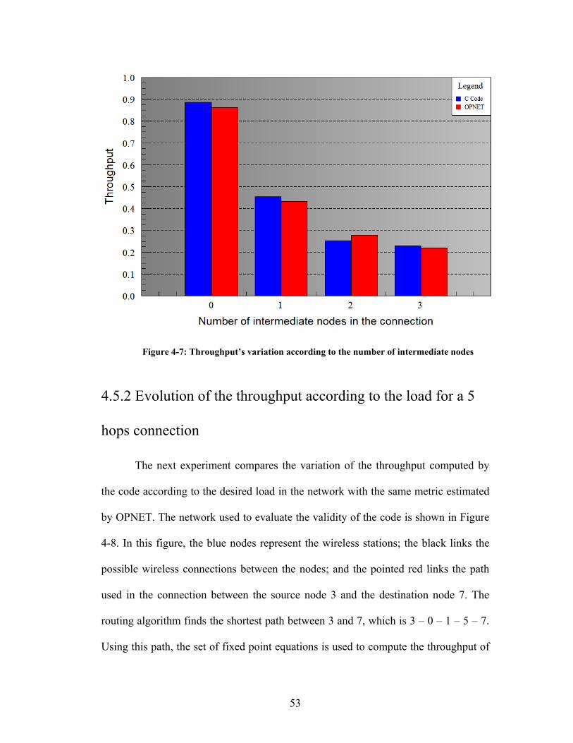
Figure 4-7: Throughput’s variation according to the number of intermediate nodes
4.5.2 Evolution of the throughput according to the load for a 5
hops connection
The next experiment compares the variation of the throughput computed by
the code according to the desired load in the network with the same metric estimated
by OPNET. The network used to evaluate the validity of the code is shown in Figure
4-8. In this figure, the blue nodes represent the wireless stations; the black links the
possible wireless connections between the nodes; and the pointed red links the path
used in the connection between the source node 3 and the destination node 7. The
routing algorithm finds the shortest path between 3 and 7, which is 3 – 0 – 1 – 5 – 7.
Using this path, the set of fixed point equations is used to compute the throughput of
53
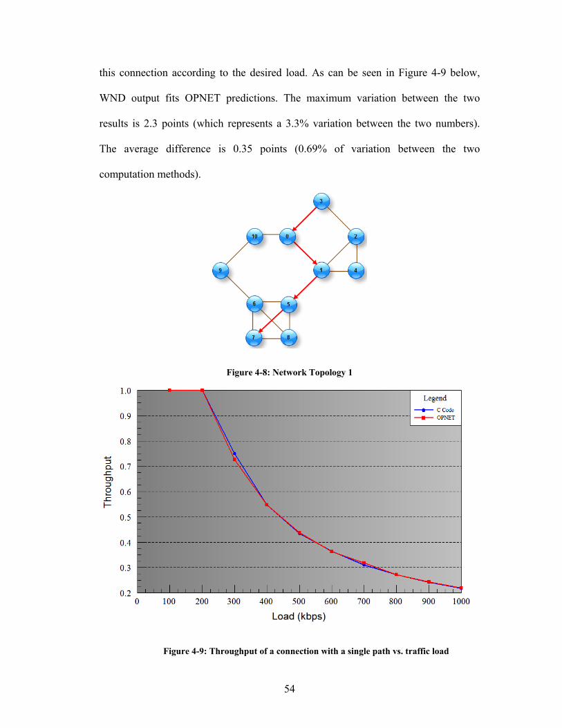
this connection according to the desired load. As can be seen in Figure 4-9 below,
WND output fits OPNET predictions. The maximum variation between the two
results is 2.3 points (which represents a 3.3% variation between the two numbers).
The average difference is 0.35 points (0.69% of variation between the two
computation methods).
Figure 4-8: Network Topology 1
Figure 4-9: Throughput of a connection with a single path vs. traffic load
54
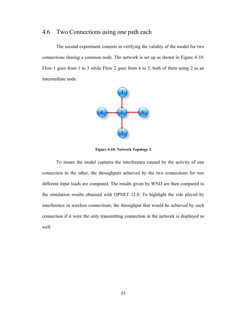
4.6 Two Connections using one path each
The second experiment consists in verifying the validity of the model for two
connections sharing a common node. The network is set up as shown in Figure 4-10.
Flow 1 goes from 1 to 3 while Flow 2 goes from 4 to 5, both of them using 2 as an
intermediate node.
Figure 4-10: Network Topology 2
To insure the model captures the interference caused by the activity of one
connection to the other, the throughputs achieved by the two connections for two
different input loads are computed. The results given by WND are then compared to
the simulation results obtained with OPNET 12.0. To highlight the role played by
interference in wireless connections, the throughput that would be achieved by each
connection if it were the only transmitting connection in the network is displayed as
well.
55
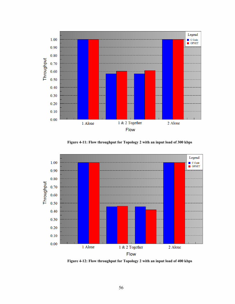
Figure 4-11: Flow throughput for Topology 2 with an input load of 300 kbps
Figure 4-12: Flow throughput for Topology 2 with an input load of 400 kbps
56
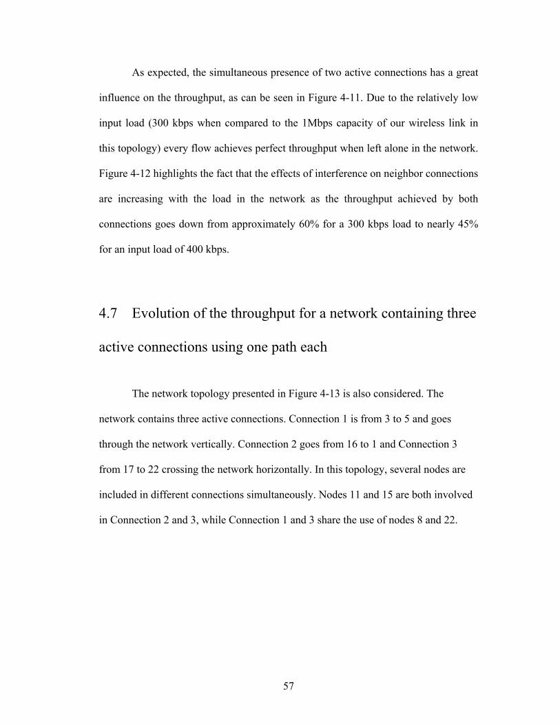
As expected, the simultaneous presence of two active connections has a great
influence on the throughput, as can be seen in Figure 4-11. Due to the relatively low
input load (300 kbps when compared to the 1Mbps capacity of our wireless link in
this topology) every flow achieves perfect throughput when left alone in the network.
Figure 4-12 highlights the fact that the effects of interference on neighbor connections
are increasing with the load in the network as the throughput achieved by both
connections goes down from approximately 60% for a 300 kbps load to nearly 45%
for an input load of 400 kbps.
4.7 Evolution of the throughput for a network containing three
active connections using one path each
The network topology presented in Figure 4-13 is also considered. The
network contains three active connections. Connection 1 is from 3 to 5 and goes
through the network vertically. Connection 2 goes from 16 to 1 and Connection 3
from 17 to 22 crossing the network horizontally. In this topology, several nodes are
included in different connections simultaneously. Nodes 11 and 15 are both involved
in Connection 2 and 3, while Connection 1 and 3 share the use of nodes 8 and 22.
57
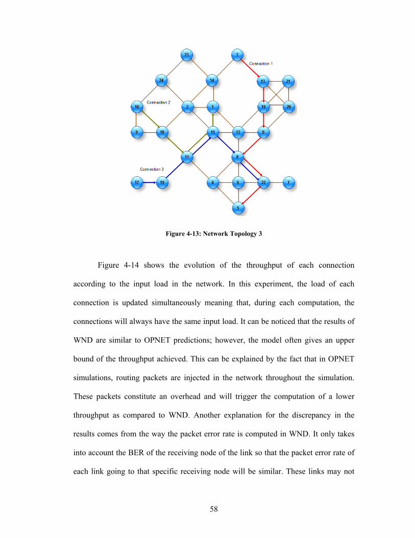
Figure 4-13: Network Topology 3
Figure 4-14 shows the evolution of the throughput of each connection
according to the input load in the network. In this experiment, the load of each
connection is updated simultaneously meaning that, during each computation, the
connections will always have the same input load. It can be noticed that the results of
WND are similar to OPNET predictions; however, the model often gives an upper
bound of the throughput achieved. This can be explained by the fact that in OPNET
simulations, routing packets are injected in the network throughout the simulation.
These packets constitute an overhead and will trigger the computation of a lower
throughput as compared to WND. Another explanation for the discrepancy in the
results comes from the way the packet error rate is computed in WND. It only takes
into account the BER of the receiving node of the link so that the packet error rate of
each link going to that specific receiving node will be similar. These links may not
58

have the same physical properties, however, so the packet error rate should also vary.
For instance, links from 15 to 8 and from 0 to 8 are different in the sense that they do
not come from the same connection of the network and they could possibly have
different packet error rates. This may explain the differences between OPNET and
WND.
Figure 4-14: Throughput of 3 connections with single path vs. traffic load
59
Chapter 5 : Throughput optimization via Probabilistic Routing
5.1 Automatic Differentiation
5.1.1 Introduction
There are many different ways to achieve differentiation of an expression
[25]. One method is to derivate symbolically an expression. The major drawback
with this method is that when used in a computer program, it is often very complex if
not impossible to resume the program to a single expression that can be derived
symbolically. Combined with the overall low speed of that method, this problem
makes symbolical derivation a non-suitable candidate for derivative computation in
computer programming. Another option would be the divided difference approach. In
this method, the following approximation is used:
( ) ( ) ( )i
i i
f x f x x f xx x
∂ + Δ −≈
∂ Δ
The problem with this method comes with how ixΔ is chosen. If ixΔ is a
small step then the approximation is going to be somewhat accurate, but if that step is
bigger, this formula does not provide a satisfactory estimate of the derivative of the
program. Moreover, that formula requires many computations for the evaluations of
higher derivatives of a function. Combined with the fact that it is impossible to
guarantee the accuracy of this method, a different scheme needs to be chosen to
compute these derivatives.
60
The last option is to use automatic differentiation. Automatic differentiation is
a numerical method to compute the derivatives of a computer program. Using the fact
that a computer program is in fact a sequence of primary operations, automatic
differentiation records the relationships between them and, using the chain rule, is
able to output very precise derivatives of a function in a short amount of time.
5.1.2 The chain rule
As stated above, automatic differentiation is based on decomposing a complex
computer program into basic operations, and then derives the whole program by using
the chain rule:
( ( ))y f g xy f gx g x
=∂ ∂ ∂
=∂ ∂ ∂
Automatic differentiation can function in two different modes: Forward Mode
or Reverse Mode.
In Forward Mode, the chain rule is traversed from left to right. Take for
instance the following expression for which the derivative according to x1 needs to be
computed:
11 2 2
2
( , ) exp( )xf x x xx
= +
This function is decomposed into different sub functions, as shown in Figure
5-1 below:
61
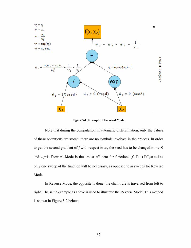
Figure 5-1: Example of Forward Mode
Note that during the computation in automatic differentiation, only the values
of these operations are stored, there are no symbols involved in the process. In order
to get the second gradient of f with respect to x2, the seed has to be changed to w1=0
and w2=1. Forward Mode is thus most efficient for functions as
only one sweep of the function will be necessary, as opposed to m sweeps for Reverse
Mode.
: ,mf m→ 1
In Reverse Mode, the opposite is done: the chain rule is traversed from left to
right. The same example as above is used to illustrate the Reverse Mode. This method
is shown in Figure 5-2 below:
62
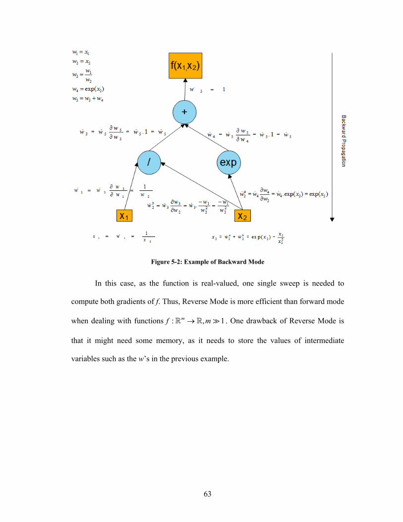
Figure 5-2: Example of Backward Mode
In this case, as the function is real-valued, one single sweep is needed to
compute both gradients of f. Thus, Reverse Mode is more efficient than forward mode
when dealing with functions . One drawback of Reverse Mode is
that it might need some memory, as it needs to store the values of intermediate
variables such as the w’s in the previous example.
: ,mf m→ 1
63

5.2 ADOL-C
There are several different programs available for automatic differentiation. In
the work by Baras [2], ADIC was used to perform automatic differentiation. In order
to employ ADIC the source code needs to be modified to fit ANSI-C standard. It is
then used by ADIC to generate another source code in which operations enabling the
computation of the derivatives are going to be interleaved with the original set of
instructions in the code. If this method generally gives better results in terms of
computing time, it generally requires a thorough change of the source code in order to
adapt it to ADIC specifications. In this case, as the code is written in C++ and the
new fixed point algorithm is a very complex implementation, such a solution is not
applicable for compatibility reasons. Consequently, automatic differentiation by
Operator Overloading in C++ was implemented using ADOL-C (Automatic
Differentiation by OverLoading in C++) [6].
Operator Overloading refers to the approach taken to compute the derivatives
in a program. It consists of changing the type of the variables involved in the
computation to a proprietary type given by the automatic differentiation tool. This
allows the tool to work on the source code and derive it based on its linked libraries.
It is then necessary to mark the section of the code which deals with the function of
interest to allow ADOL-C to record the sequence of operations taking place in this
section so that the derivatives of interest can be computed. ADOL-C then produces a
tape of this section. This is an internal representation of the marked section used to
compute the derivatives. The main concern here is the memory used. One can predict
that, if a marked section is requiring many iterations to compute the output, the
64

associated tape will record several operations and use a significant amount of
memory. The advantage of ADOL-C is that it enables the choice of Forward or
Reverse Mode and provides appropriate drivers specially adapted to optimization
problems, differential equations, or the computation of Hessians and Jacobians. This
method is compatible with C++ and permits implementation with little change to the
program, but it is slower than source code transformation tool due to its inefficiency
in code optimization.
5.3 Methodology: Gradient Projection
Here, the method employed to optimize the overall throughput in the network
by changing the path probability distribution of each connection on the network is
presented. Note Pc the set of paths used in connection c and C the set of all active
connections in the network. Then the total throughput T is:
,
,
c
c
c last pc p P
c first pc p P
Tα λ
α λ
∈ ∈
∈ ∈
⎛ ⎞⎜ ⎟⎜ ⎟⎝ ⎠=⎛ ⎞⎜ ⎟⎜ ⎟⎝ ⎠
∑ ∑
∑ ∑
C
C
Here, αc’s are used as weights to control the optimization of the overall
network throughput. By default, these coefficients are set to 1 for each active data
connection in the network, 2 for voice connections and 3 for video connections so as
to permit the most critical communications to be optimized primarily. Assuming there
are m = C active connections in the network, nc paths used in the connection c and
noting πi,c the probability associated with using path i in connection c, the total
throughput is a function of these input probabilities, namely:
65
1 111, , ,( ,..., ,..., )c cmc n c n cT T π π π=
m
Thus, the optimization problem can be written in the following way:
1 11
c
1, , ,
,i
,
max ( ,..., ,..., )
. 1,
0, ( , )
c cmc n c n c
i cP
i c c
T T
s t c
i c P
π π π
π
π∈
=
= ∀ ∈
≥ ∀ ∈ ×
∑m
C
C
To solve this optimization problem, the gradient projection method will be
applied. This tool is commonly used in engineering design problems. This solution is
particularly adapted to the problem here because there is a need to compute the
gradients of the throughput according to the input routing probabilities in order to be
able to maximize it. In addition, those gradients need to be projected on the constraint
space to obtain results fulfilling the given constraints. Naming c∇ the average
gradient obtained for connection c, that value needs to be subtracted from each of the
gradients obtained for the paths in Pc to make sure the constraintc
,i
1i cP
π∈
=∑ is met.
In other words, at each iteration the set of routing probabilities will be updated
using the following formula:
, ,,
max 0, , 0,..., k k k
k
i c i c ci c
T k mπ π βπ
⎛ ⎞⎛ ⎞∂⎜ ⎟= + −∇ ∀ ∈⎜ ⎟⎜ ⎟⎜ ⎟∂⎝ ⎠⎝ ⎠
In this formula, β is a parameter used to control the size of the steps taken
during the update process of each iteration. If β is too big, it will not be possible to
find the overall maximum of the function. The program will oscillate around it
because of the inappropriate size of the update step. Whenever WND detects that the
optimization algorithm in fact provided a result smaller than the one computed during
66
the previous iteration, β is updated using the following scheme:
min if 2ββ β β← ≥ where βmin represents the smallest step accepted in the program.
This βmin has been introduced to insure a fast convergence of the algorithm. In the
case of many oscillations, a very fast decrease in β can be experienced leading to a
very slow update process and a long convergence time for the program. This iteration
is continued for each connection until every path having a non-nil probability of
being used has the same gradient as the other non-nil paths for the same connection.
Namely, the iteration stops when:
,,
0 , in each ci c ci c
TP cππ∂
∀ ≠ ∈ = ∇ ∈∂
C
Once this algorithm has converged, a new set of results for the network
configuration can be displayed, containing:
1. The optimized throughput of each active connection in the network.
2. The set of routing probabilities for each connection needed in order to
achieve such throughput.
67
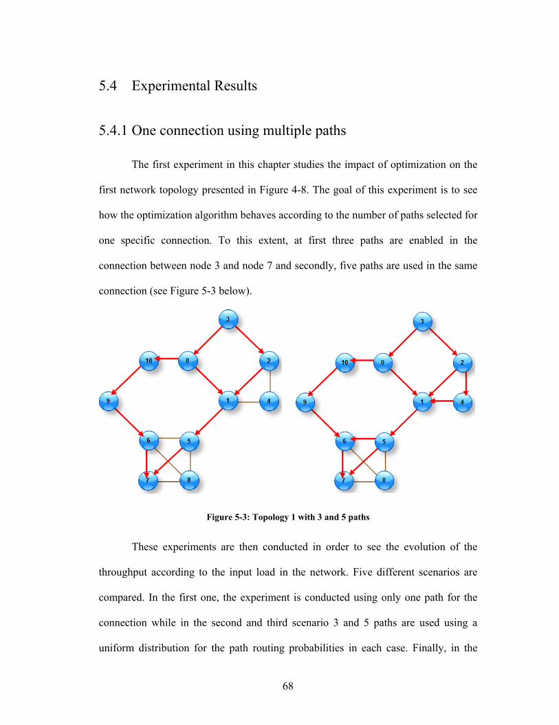
5.4 Experimental Results
5.4.1 One connection using multiple paths
The first experiment in this chapter studies the impact of optimization on the
first network topology presented in Figure 4-8. The goal of this experiment is to see
how the optimization algorithm behaves according to the number of paths selected for
one specific connection. To this extent, at first three paths are enabled in the
connection between node 3 and node 7 and secondly, five paths are used in the same
connection (see Figure 5-3 below).
Figure 5-3: Topology 1 with 3 and 5 paths
These experiments are then conducted in order to see the evolution of the
throughput according to the input load in the network. Five different scenarios are
compared. In the first one, the experiment is conducted using only one path for the
connection while in the second and third scenario 3 and 5 paths are used using a
uniform distribution for the path routing probabilities in each case. Finally, in the
68
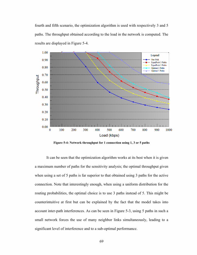
fourth and fifth scenario, the optimization algorithm is used with respectively 3 and 5
paths. The throughput obtained according to the load in the network is computed. The
results are displayed in Figure 5-4.
Figure 5-4: Network throughput for 1 connection using 1, 3 or 5 paths
It can be seen that the optimization algorithm works at its best when it is given
a maximum number of paths for the sensitivity analysis; the optimal throughput given
when using a set of 5 paths is far superior to that obtained using 3 paths for the active
connection. Note that interestingly enough, when using a uniform distribution for the
routing probabilities, the optimal choice is to use 3 paths instead of 5. This might be
counterintuitive at first but can be explained by the fact that the model takes into
account inter-path interferences. As can be seen in Figure 5-3, using 5 paths in such a
small network forces the use of many neighbor links simultaneously, leading to a
significant level of interference and to a sub-optimal performance.
69
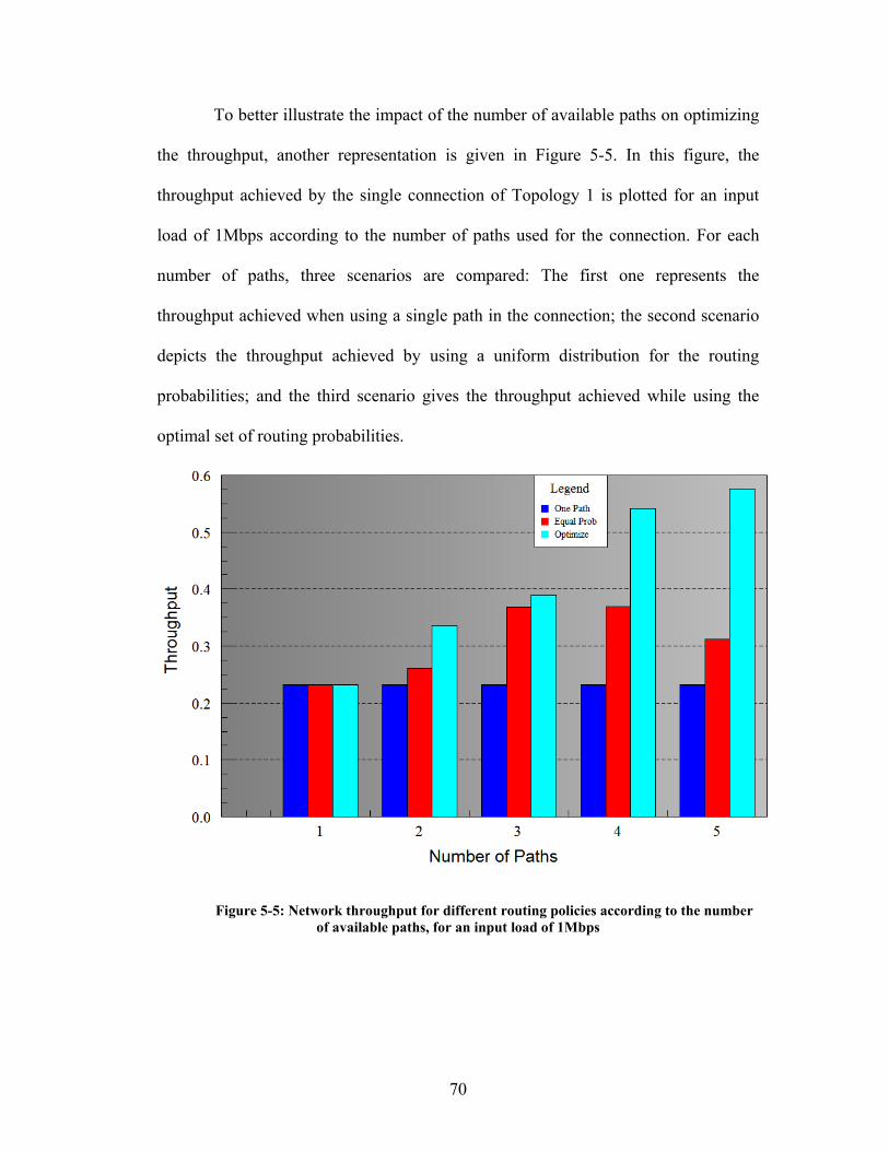
To better illustrate the impact of the number of available paths on optimizing
the throughput, another representation is given in Figure 5-5. In this figure, the
throughput achieved by the single connection of Topology 1 is plotted for an input
load of 1Mbps according to the number of paths used for the connection. For each
number of paths, three scenarios are compared: The first one represents the
throughput achieved when using a single path in the connection; the second scenario
depicts the throughput achieved by using a uniform distribution for the routing
probabilities; and the third scenario gives the throughput achieved while using the
optimal set of routing probabilities.
Figure 5-5: Network throughput for different routing policies according to the number of available paths, for an input load of 1Mbps
70
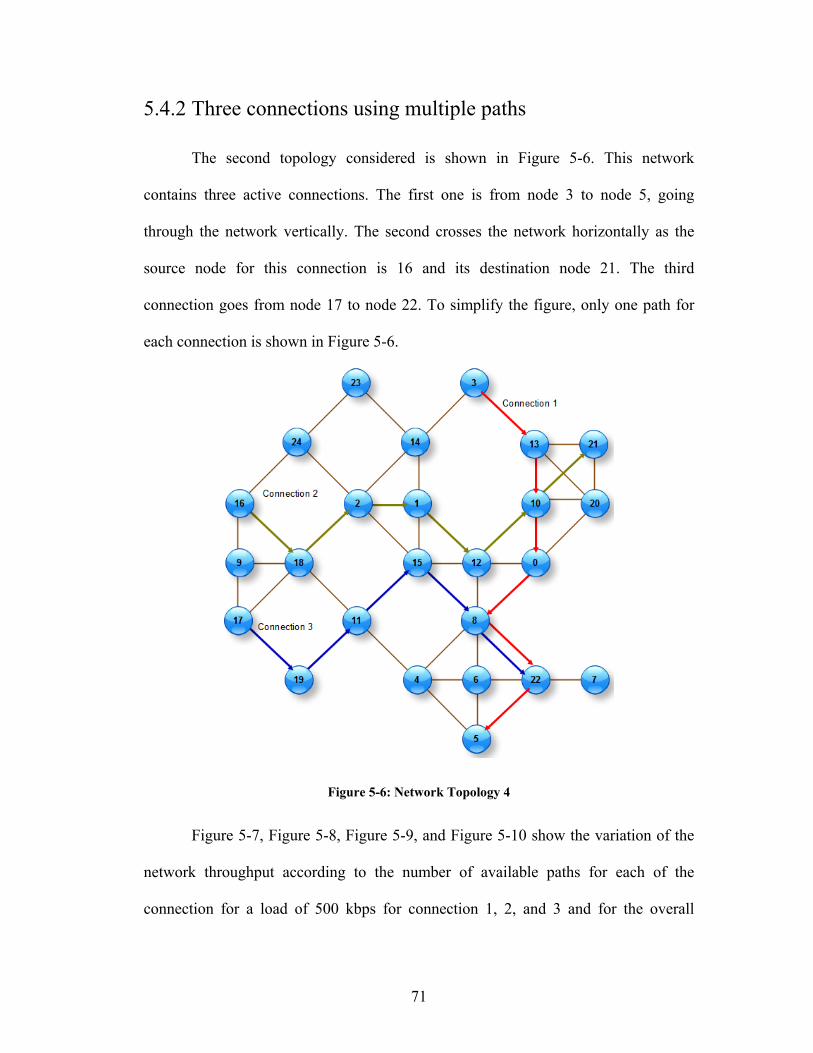
5.4.2 Three connections using multiple paths
The second topology considered is shown in Figure 5-6. This network
contains three active connections. The first one is from node 3 to node 5, going
through the network vertically. The second crosses the network horizontally as the
source node for this connection is 16 and its destination node 21. The third
connection goes from node 17 to node 22. To simplify the figure, only one path for
each connection is shown in Figure 5-6.
Figure 5-6: Network Topology 4
Figure 5-7, Figure 5-8, Figure 5-9, and Figure 5-10 show the variation of the
network throughput according to the number of available paths for each of the
connection for a load of 500 kbps for connection 1, 2, and 3 and for the overall
71
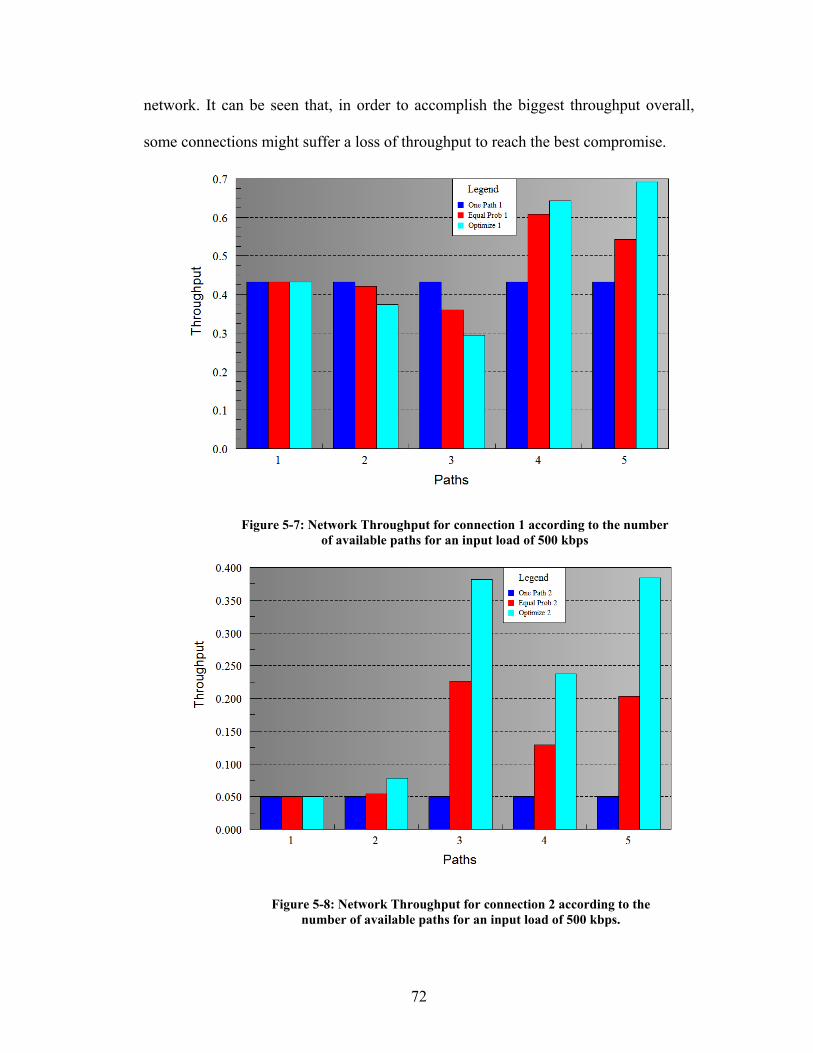
network. It can be seen that, in order to accomplish the biggest throughput overall,
some connections might suffer a loss of throughput to reach the best compromise.
Figure 5-7: Network Throughput for connection 1 according to the number of available paths for an input load of 500 kbps
Figure 5-8: Network Throughput for connection 2 according to the number of available paths for an input load of 500 kbps.
72
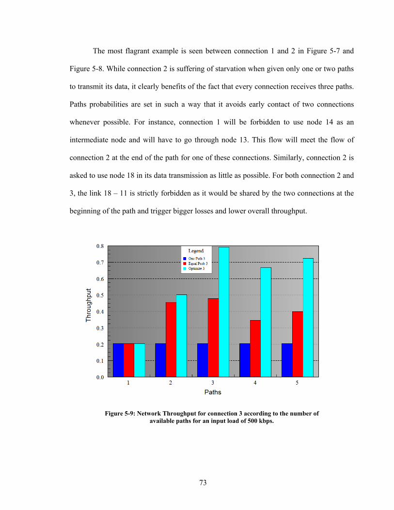
The most flagrant example is seen between connection 1 and 2 in Figure 5-7 and
Figure 5-8. While connection 2 is suffering of starvation when given only one or two paths
to transmit its data, it clearly benefits of the fact that every connection receives three paths.
Paths probabilities are set in such a way that it avoids early contact of two connections
whenever possible. For instance, connection 1 will be forbidden to use node 14 as an
intermediate node and will have to go through node 13. This flow will meet the flow of
connection 2 at the end of the path for one of these connections. Similarly, connection 2 is
asked to use node 18 in its data transmission as little as possible. For both connection 2 and
3, the link 18 – 11 is strictly forbidden as it would be shared by the two connections at the
beginning of the path and trigger bigger losses and lower overall throughput.
Figure 5-9: Network Throughput for connection 3 according to the number of available paths for an input load of 500 kbps.
73
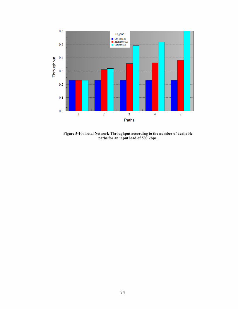
Figure 5-10: Total Network Throughput according to the number of available paths for an input load of 500 kbps.
74
Chapter 6 : Conclusions and Future Work
6.1 Conclusion
This work presented a new method for performance analysis of 802.11
wireless networks. The tool enables end-to-end network design. Given a network
description, it outputs a set of paths for each active connection. It then computes the
throughput of multiple connections in a network by using a fixed point algorithm. The
main contribution of this work for performance modeling of 802.11 is that it allows
paths to share common nodes. To compute the best trade-off for network design, the
tool also performs sensitivity analysis using automatic differentiation. In this thesis,
an example of the efficiency of that method was shown by computing the derivatives
of the total throughput according to the path routing probabilities of each connection.
Gradient projection has been chosen to optimize the path routing distribution so as to
achieve the highest network throughput. Network topologies have been set up for
different purposes. The validity of the fixed point algorithm was first demonstrated by
running parallel experiments both on WND and on a discrete event simulator,
OPNET 12.0. The main advantage of the tool over discrete events simulation
platforms such as OPNET is clearly the computation time. While WND converges on
the order of seconds, OPNET often requires several minutes to compute the
throughput in a network. This makes the model more adapted to compute
approximations of throughput in emergency situations. Table 6-1 compares the time
75
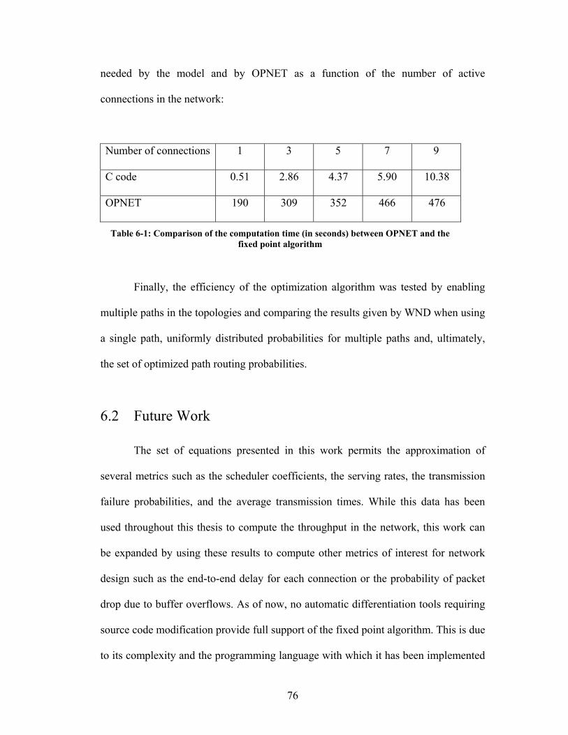
needed by the model and by OPNET as a function of the number of active
connections in the network:
Number of connections 1 3 5 7 9
C code 0.51 2.86 4.37 5.90 10.38
OPNET 190 309 352 466 476
Table 6-1: Comparison of the computation time (in seconds) between OPNET and the fixed point algorithm
Finally, the efficiency of the optimization algorithm was tested by enabling
multiple paths in the topologies and comparing the results given by WND when using
a single path, uniformly distributed probabilities for multiple paths and, ultimately,
the set of optimized path routing probabilities.
6.2 Future Work
The set of equations presented in this work permits the approximation of
several metrics such as the scheduler coefficients, the serving rates, the transmission
failure probabilities, and the average transmission times. While this data has been
used throughout this thesis to compute the throughput in the network, this work can
be expanded by using these results to compute other metrics of interest for network
design such as the end-to-end delay for each connection or the probability of packet
drop due to buffer overflows. As of now, no automatic differentiation tools requiring
source code modification provide full support of the fixed point algorithm. This is due
to its complexity and the programming language with which it has been implemented
76

(C++). Further studies of automatic differentiation tools could lead to better
performance of the model. Automatic differentiation by operator overloading does
not optimize the code and exhibits a longer response time than tools requiring source
code transformation. Finally, another interesting extension to this work would be to
include the computation of the physical layer error rate within the model. This would
avoid requesting previously computed values.
77
Bibliography [1] F.P. Kelly, “Loss Networks”, The Annals of Applied Probability, vol.1, no.3, pp. 319-378, Aug. 1991. [2] J. S. Baras, V. Tabatabaee, G. Papageorgiou, N. Rentz, Y. Shang, “Loss Model Approximations and Sensitivity Computations for Wireless Network Design”, MILCOM 2007. [3] D. Mitra, J.A. Morrison and K. G. Ramakrishnan, “ATM network design and optimization: A multirate loss network framework”, IEEE/ACM Trans. Networking, vol. 4, no. 4, pp. 531-543, Aug. 1996. [4] S. Chung, A. Kashper and K. W. Ross, “Computing approximate blocking probabilities for large loss networks with state-dependent routing”, IEEE/ACM Trans. Networking, vol. 1, no. 1, pp. 105-115, Feb. 1993. [5] M. Liu and J. S. Baras, “Fixed point approximation for multirate multihop loss networks with adaptive routing”, IEEE ACM Trans. Networking, vol. 12, no. 2, pp 361-374, Apr. 2004. [6] ADOL-C, Automatic Differentiation by OverLoading in C++, URL: http://www.math.tu-dresden.de/~adol-c/ [7] OPNET Modeler, URL: http://opnet.com [8] A. S. Tanenbaum, “Computer Networks”, Fourth Edition, page 294, 2002. [9] Wikipedia contributors, “Direct-sequence spread spectrum”, Wikipedia, The Free Encyclopedia, http://en.wikipedia.org/w/index.php?title=Direct-sequence_spread_spectrum&oldid=153334333 [10] A. S Tanenbaum, “Computer Networks”, Fourth Edition, pages 164-165, 2002. [11] Wikipedia contributors, “Orthogonal frequency-division multiplexing”, Wikipedia, The Free Encyclopedia, http://en.wikipedia.org/w/index.php?title=Orthogonal_frequency-division_multiplexing&oldid=156049525 [12] A. S Tanenbaum, “Computer Networks”, Fourth Edition, pages 296-297, 2002. [13] A. S Tanenbaum, “Computer Networks”, Fourth Edition, page 297 – Figure 4-27, 2002.
78
[14] A. S. Tanenbaum, “Computer Networks”, Fourth Edition, page 299 – Figure 4-29, 2002. [15] G. Bianchi. “Performance Analysis of the IEEE 802.11 Distributed Coordination Function”, IEEE Journal on Selected Area in Comm. Vol. 18, No 3, March 2000. [16] K. Medepalli and F. A. Tobagi, “Towards Performance Modeling of IEEE 802.11 based Wireless Networks: A Unified Framework and its Applications”, in INFOCOM, Barcelona, 2006. [17] M. M. Hira, F. A. Tobagi, K. Medepalli, “Throughput Analysis of a Path in an IEEE 802.11 Multihop Wireless Network”, Wireless Communications and Networking Conference, 2007. [18] Y. Gao, D.-M. Chiu, J. C. S. Lui, “Determining the End-to-end Throughput Capacity in Multi-Hop Networks: Methodology and Applications”, in Proceedings of SIGMETRICS: Joint International Conference in Measurement and Modeling of Computer Systems, 2006, pp. 30-36. [19] M. Chiang, S. H. Low, R. A. Calderbank, and J. C. Doyle, “Layering as Optimization Decomposition”, Proceedings of IEEE, 2006. [20] E. L Lawler, “Combinatorial Optimization: Networks and Matroids”. Holt, Rinehart, and Winston, New York, 1976. [21] X. Wang and K. Kar, “Throughput Modelling and Fairness Issues in CSMA/CA Based Ad-Hoc Networks”, in Proc. IEEE INFOCOM, Miami, FL,USA, 2005 [22] M. Garetto, T. Salonidis, and E. Knightly, “Modeling per-flow throughput and capturing starvation in CSMA multi-hop wireless networks”, in Proc. IEEE INFOCOM, Barcelona, Spain, 2006 [23] Wikipedia contributors, “Fixed point iteration”, Wikipedia, The Free Encyclopedia, http://en.wikipedia.org/w/index.php?title=Fixed_point_iteration&oldid=144272300 [24] Wikipedia contributors, “Fixed point (mathematics)”, Wikipedia, The Free Encyclopedia, http://en.wikipedia.org/w/index.php?title=Fixed_point_%28mathematics%29&oldid=153378978 [25] Wikipedia contributors, “Automatic differentiation”, Wikipedia, The Free Encyclopedia, http://en.wikipedia.org/w/index.php?title=Automatic_differentiation&oldid=155661486
79