1

Throughput Optimal Switching inMulti-channel WLANs

Qingsi Wang and Mingyan Liu

Abstract—We observe that in a multi-channel wireless system, an opportunistic channel/spectrum access scheme that solelyfocuses on channel quality sensing measured by received SNR may induce users to use channels that, while providing bettersignals, are more congested. Ultimately the notion of channel quality should include both the signal quality and the level ofcongestion, and a good multi-channel access scheme should take both into account in deciding which channel to use and when.Motivated by this, we focus on the congestion aspect and examine what type of dynamic channel switching schemes may resultin the best system throughput performance. Specifically we derive the stability region of a multi-user multi-channel WLAN systemand determine the throughput optimal channel switching scheme within a certain class of schemes. We also empirically examinethe impact of considering congestion in addition to signal quality in making channel selection decisions.

Index Terms—Wireless LAN, 802.11 DCF, multi-channel wireless system, channel switching policy, stability region, throughputoptimality

!

1 INTRODUCTIONAdvances in software defined radio in recent yearshave motivated numerous studies on building agile,channel-aware transceivers that are capable of sensinginstantaneous channel quality [1], [2], [3]. With thisopportunity comes the challenge of making effec-tive opportunistic channel access and transmissionscheduling decisions, as well as designing support-ing system architectures. There have been extensivestudies on dynamic channel access in a multi-user,multi-channel wireless system, see e.g., [4], [5]. Byallowing users to dynamically select which channel touse for transmission, these schemes aim to improvethe system performance, typically measured by thetotal (or per user) throughput, the average packetdelay and etc, compared to a system with a singlechannel or more static channel allocations. The mainreason behind such improvement lies in temporal,spatial and spectral diversity. That is, the quality ofa channel perceived by a user is time-varying, user-dependent, and channel-dependent.

Within this context we make the additional obser-vation that there is also a congestion diversity in thata channel with fewer number of competing userspresents better quality for a user. This is particularlytrue in a random access setting, where a large numberof competing users can induce large backoff timervalues that in turn lead to longer waiting time andlower throughput. We note that in a multi-channelsystem, an opportunistic access scheme that solelyfocuses on channel quality sensing as a result of

• Q. Wang and M. Liu are with the Department of Electrical Engineeringand Computer Science, University of Michigan, Ann Arbor, MI 48109.

This work is supported by NSF grant CIF-0910765, ARO grant W911NF-11-1-0532, and NASA grant NNX09AE91G.

random fading and shadowing, e.g., by measuringreceived SNR [6], [5], may induce users to use chan-nels that, while providing better signals, are morecongested. This can reduce the expected performancegain, or even turn gain to loss. Ultimately the notionof “channel quality” should include both the signalquality and the level of congestion, and a good multi-channel access scheme should take both into accountin deciding which channel to use and when.

Motivated by the above, in this study we examinethe possibility of utilizing congestion diversity to pro-mote certain performance measures, e.g., throughput.As mentioned above, our ultimate goal is to constructan opportunistic channel access scheme that is awareof both signal quality and user congestion. However,in the present paper we will primarily limit ourattention to addressing the congestion aspect only.We do provide numerical results on the impact ofconsidering congestion in addition to signal qualityin making channel selection decisions.

Specifically, we ask the question of what type ofdynamic channel switching schemes will give thebest performance in a multi-channel WLAN. This willbe evaluated using the notion of stability region ofa scheme. This is because more effective resourceallocation and sharing can achieve a lower overallcongestion level, thus expanding the range of sustain-able arrival rates and resulting in a larger stabilityregion. The scheme with the largest such region iscommonly known as the throughput optimal scheme.With this objective, we set out to study the stabilityregion of a multi-channel WLAN system where usersare allowed to dynamically switch between channels.

The main contributions of this paper are as follows.• A mean-field based model is constructed to char-

acterize the stability region of a multi-channel

2

WLAN system. We show that the size of the back-off window plays a decisive role in shaping thecorresponding stability region: when the backoffwindow is sufficiently large, the stability regionis convex; as the window size decreases it evolvesinto a concave region.

• Using this mean-field model, we provide an an-alytical justification of using channel-switchingpolicies that achieve load balance in systems withsymmetric channels. This is then extended tosystems with asymmetric channels.

• We propose several simple heuristic implementa-tions of the channel-switching policies presentedin this paper.

802.11 DCF has been very extensively studied inthe literature, ranging from throughput performancein the saturated regime [7], [8] and the non-saturatedregime [9], [10], to its rate region [11], [12], to channelassignment in multi-channel WLANs [13], [14], toname a few. To the best of our knowledge, however,none has studied multi-channel WLAN in the con-text of stability region. Works most relevant to oursinclude ones on the stability region of slotted Aloha(e.g., [15]) and the rate region of 802.11 DCF [11], [12].

In the remainder of the paper, we first introduce asystem of equations to characterize the stability regionof a single channel WLAN consisting of multipleusers within a single interference domain (Section 3)followed by numerical results (Section 4). We thenextend the same method to characterize the stabilityregion of a multi-channel system and use this result todetermine the throughput optimal channel switchingschemes within a class (Section 5). We also discusshow such schemes may be implemented in practice(Section 6). Due to the space limit, some technicaldetails are omitted and may be found in our technicalreport [16].

2 SYSTEM MODEL AND PRELIMINARIES

Consider a multiple access system using the IEEE802.11 DCF. There are N nodes (or users interchange-ably), indexed by the set N = {1, 2, . . . , N}, each withan infinite buffer, one transceiver (i.e., a single wirelessinterface) and uses the same parameterization. Weassume the channel is ideal and there is no MAC-levelpacket discard, i.e., there is no retransmission limit ofa packet after collision. Throughout the analysis wealso adopt a few other simplifying assumptions tomake the problem tractable; these will be stated in thecontext to which they apply. It should be noted thatdue to the complexity of the problem, successive sim-plification in the modeling effort is a rather commonpractice and has been used in most if not all previousworks. We later show that these simplifications donot impact the accuracy of the model under normaloperating parameter values.

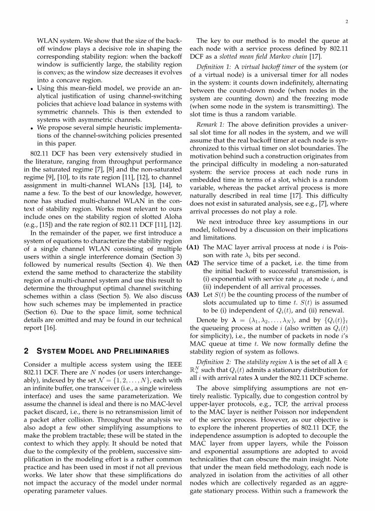
The key to our method is to model the queue ateach node with a service process defined by 802.11DCF as a slotted mean field Markov chain [17].

Definition 1: A virtual backoff timer of the system (orof a virtual node) is a universal timer for all nodesin the system: it counts down indefinitely, alternatingbetween the count-down mode (when nodes in thesystem are counting down) and the freezing mode(when some node in the system is transmitting). Theslot time is thus a random variable.

Remark 1: The above definition provides a univer-sal slot time for all nodes in the system, and we willassume that the real backoff timer at each node is syn-chronized to this virtual timer on slot boundaries. Themotivation behind such a construction originates fromthe principal difficulty in modeling a non-saturatedsystem: the service process at each node runs inembedded time in terms of a slot, which is a randomvariable, whereas the packet arrival process is morenaturally described in real time [17]. This difficultydoes not exist in saturated analysis, see e.g., [7], wherearrival processes do not play a role.

We next introduce three key assumptions in ourmodel, followed by a discussion on their implicationsand limitations.

(A1) The MAC layer arrival process at node i is Pois-son with rate !i bits per second.

(A2) The service time of a packet, i.e. the time fromthe initial backoff to successful transmission, is(i) exponential with service rate µi at node i, and(ii) independent of all arrival processes.

(A3) Let S(t) be the counting process of the number ofslots accumulated up to time t. S(t) is assumedto be (i) independent of Qi(t), and (ii) renewal.

Denote by ! = (!1,!2, . . . ,!N ), and by {Qi(t)}tthe queueing process at node i (also written as Qi(t)for simplicity), i.e., the number of packets in node i’sMAC queue at time t. We now formally define thestability region of system as follows.

Definition 2: The stability region ! is the set of all ! !RN

+ such that Qi(t) admits a stationary distribution forall i with arrival rates ! under the 802.11 DCF scheme.

The above simplifying assumptions are not en-tirely realistic. Typically, due to congestion control byupper-layer protocols, e.g., TCP, the arrival processto the MAC layer is neither Poisson nor independentof the service process. However, as our objective isto explore the inherent properties of 802.11 DCF, theindependence assumption is adopted to decouple theMAC layer from upper layers, while the Poissonand exponential assumptions are adopted to avoidtechnicalities that can obscure the main insight. Notethat under the mean field methodology, each node isanalyzed in isolation from the activities of all othernodes which are collectively regarded as an aggre-gate stationary process. Within such a framework the

3

packet service time is taken to be stationary (see e.g.,Bianchi’s well-known mean field Markovian model ofthe service process [7]).

With A1 and A2, Qi(t) is then a well-definedM/M/1 queue, and for a given !, ! ! ! if and onlyif Qi(t) is positive recurrent. Equivalently we mayconsider the utilization factor "i at node i, given by"i = min{!i

µi, 1}: the queue is stable if and only if

"i < 1. If Qi(t) is positive recurrent, then it is ergodicand we have limt!" P (Qi(t) > 0) = 1 " #i(0) = "i,where #i is the stationary distribution of Qi(t). If Qi(t)is transient or null recurrent, in which case "i = 1, wehave limt!" P (Qi(t) = 0) = 0 = 1 " "i. Therefore, "iis asymptotically given by limt!" P (Qi(t) > 0) in allcases in our model.

For technical reasons we will also consider the em-bedded queueing process Q̂i(n), n = 1, 2, · · · , definedas Q̂i(n) := Qi(Tn), where Tn is the time of the nthslot boundary. Q̂i(n) is thus a discrete-time processconstructed by observing Qi(t) at slot boundaries.

For an arbitrary process S(t), Q̂i(n) is not nec-essarily Markovian. However, given assumption A3,durations between slot boundaries are i.i.d., constitut-ing sampling periods that are independent of Qi(t).Hence Q̂i(t) is a discrete-time Markov chain underour assumption. It’s worth noting that A3 does notexactly hold in reality because the slot length is afunction of a node’s activity, and thus the state ofits queue, even with the mean field simplification ofother nodes’ behavior (this is more precisely shownin the appendix). However, this dependence weakenswhen the number of nodes or the backoff windowsize is sufficiently large. We empirically show that thisassumption does not impact the accuracy of predic-tion even with a small node population and backoffwindow size.

Let "̂i denote the utilization factor under thediscrete-time system Q̂i(n). In general "̂i #= "i. Indeedwe show in Appendix A that "̂i $ "i where equalityholds if and only if "i = 1 or "i = 0, i.e., node i iseither saturated or idle. Similar to "i, "̂i is asymptot-ically given by limn!" P (Q̂i(n) > 0).

We will adopt Bianchi’s decoupling approximation[7] as another key assumption, stated as follows.Define Ci(j) := 1 if the jth attempt by node i resultsin a collision, and Ci(j) := 0 if it results in a success.

(A4) [Bianchi’s Decoupling Approximation] For eachnode i ! N , the collision sequence {Ci(j)} is i.i.d.with P (Ci(j) = 1) = pi for some constant pi.

In reality successive attempts by the same node mayoccur if it repeatedly selects timer value 0 while othernodes’ timers remain frozen. In such cases the aboveassumption ceases to hold. This phenomenon can beprominent when the window size is small, and hasbeen taken into account in some recent work [18]. Inthis study we will ignore the possibility of successiveattempts for simplicity of presentation and adopt

(A4). (A more precise model is possible by imposingindependence not on all attempts but only the firstattempt in each such sequence.) This is reasonablewhen the initial window size is sufficiently large.Our empirical results are fairly close between withand without consideration of successive attempts forlarge backoff windows. For small backoff windows,the discrepancy between the two will be illustrated inthe numerical results.

We will use the term backoff length to mean thetotal number of slots that a node spends between twosuccessive timer renewals during the service process,which is the selected timer value plus 1. Define Ns

i

and N txi , respectively, as the numbers of slots and

transmission attempts that node i takes in servingone packet. W i :=

E[Nsi ]

E[Ntxi ] is referred to as the average

backoff length of node i.Using Bianchi’s approximation, we have

E[Nsi ] =

"!

k=0

k!

j=0

2min{j,m}W + 1

2(pi)

k(1" pi)

="!

j=0

2min{j,m}W + 1

2

" "!

k=j

(pi)k(1" pi)

#

="!

j=0

2min{j,m}W + 1

2(pi)

j

where W is the size of the initial backoff window andm is the value of the maximum backoff stage. Alsonote E[N tx

i ] = 11#pi

. Therefore, W i is given by

W i =1

2

$W

"(1" pi)

m#1!

j=0

(2pi)j + (2pi)

m

#+ 1

%.

We next derive a relationship between the trans-mission attempt probability and "̂i. Let $i(n) be theprobability that node i initiates a transmission attemptin the nth slot.

Lemma 1: $i := limn!" $i(n) exists and is given by$i = "̂i/W i.

Proof: Let TX(n) denote the event that node iinitiates an attempt in the nth slot. Then

$i(n) = P (TX(n)|Q̂i(n) > 0) · P (Q̂i(n) > 0)+

+ P (TX(n)|Q̂i(n) = 0) · P (Q̂i(n) = 0).

Consider now the sequence of slots in which node ihas a packet in service. Given the decoupling amongnodes, the occurrences of slots in which node i startsthe service for a packet thus form renewal events. Re-garding each transmission attempt as one-unit rewardand using the renewal reward theory, we then obtain

limn!"

P (TX(n)|Q̂i(n) > 0) =E[N tx

i ]

E[Nsi ]

=1

W i.1

1. We note that [19] used a similar technique in computing theconditional transmission probability defined therein.

4

Since limn!" P (Q̂i(n) > 0) = "̂i, andP (TX(n)|Q̂i(n) = 0) = 0, the result follows.

To put the above result in context, one easily verifiesthat in the extreme case where all nodes are saturatedand identical, we have "̂i = "i = " = 1 and pi = p forall i. Consequently,

$i = $ =2

W&(1" p)

'm#1j=0 (2p)j + (2p)m

(+ 1

=2(1" 2p)

(1" 2p)(W + 1) + pW (1" (2p)m),

which is exactly the same as obtained in [7] Eqn (7).

3 SINGLE CHANNEL STABILITY REGION3.1 The stability region equation "

Our first main result is the following theorem on thequantitative description of !. Let E[Si,Q,Tx

] denotethe conditional average length of a slot given thatthe queue at node i is non-empty but i does nottransmit in this slot. Ts and Tc denote the lengths ofa successful transmission and a collision, respectively.

Theorem 1: ! ! ! if and only if there exists atleast one solution " = ($1, $2, . . . , $N ) to the followingconstrained system of equations (",C,!):

" :

)***********+

***********,

$i ="̂iW i

, %i (a)

pi = 1"-

j $=i

(1" $j), %i (b)

"i = min

.!i

P

"W i " 1

1" piE[Si,Q,Tx

] +

+ Tcpi

1" pi+ Ts

#, 1

/, %i (c)

subject to

C :

.0 $ $i $ 1, %i (i)0 $ "i < 1, %i (ii)

where P is the packet payload size.Proof: "(a) is the result of Lemma 1, and "(b) is

an immediate consequence of the definition of pi. Letthe average service time at node i be Xi seconds perbit; the average service time per packet is thus PXi.Define Y i(j) as

Y i(j) = Tc +

"2min{j,m}W + 1

2" 1

#E[Si,Q,Tx

].

Physically, Y i(j) is the average time between the be-ginning of the jth transmission attempt, which resultsin a collision, and the beginning of the (j + 1)thattempt, given that node i encounters at least j col-lisions before completing the service of some packet.Since the collision sequence is geometric, we have

PXi ="!

k=0

$"W + 1

2" 1

#E[Si,Q,Tx

] +k!

j=1

Y i(j)+

+ Ts

%& (pi)

k(1" pi)

="!

j=1

"!

k=j

Y i(j)(pi)k(1" pi) +

"W + 1

2" 1

#&

& E[Si,Q,Tx] + Ts

="!

j=1

(pi)jY i(j) +

"W + 1

2" 1

#E[Si,Q,Tx

] + Ts.

Therefore,

PXi ="!

j=1

$(pi)

j

"Tc +

"2min{j,m}W + 1

2" 1

#&

& E[Si,Q,Tx]

#%+

"W + 1

2" 1

#E[Si,Q,Tx

] + Ts

="!

j=0

$2min{j,m}W " 1

2(pi)

j

%E[Si,Q,Tx

]+

+ Tc

"!

j=1

(pi)j + Ts

=W i " 1

1" piE[Si,Q,Tx

] + Tcpi

1" pi+ Ts.

Note that $i < 1 for all i, and we have pi < 1 for all ias a result. In addition, E[Si,Q,Tx

] is finite (computedin the appendix). Hence we conclude that the packetservice time is finite. Thus, the utilization factor ofnode i is given by "i = min{!iXi, 1} and "(c) follows.C(i) is for the validity of $ as a probability measure.(", C(i), !) then constitutes a full description on thesystem utilization. C(ii) is the necessary and sufficientcondition for stability as commented in the previoussection.

For a given set of system parameter values, twosets of quantities are needed to compute ": E[Si,Q,Tx

]and "̂i, %i ! N . These are computed in Appendix Band C, respectively. In particular, in Appendix C weshow that though it is analytically intractable, "̂i iswell approximated by

"̂i '"iE[Si,Q]

"iE[Si,Q] + (1" "i)E[Si,Q],

where E[Si,Q] (resp. E[Si,Q]) is the conditional averagelength of a slot given that the queue at node i is non-empty (resp. empty) at the beginning of this slot.

3.2 Characterizing the solutions to "

Without the stability constraint C(ii), (", C(i), !) canbe rewritten as a vector equation in [0, 1]N , " = !(" ),where " = ($1, $2, . . . , $N ) ! [0, 1]N , and the existenceof solutions can be shown by Brouwer’s fixed pointtheorem. However, the uniqueness of its solution isin general difficult to prove; nevertheless, under thecondition of a sufficiently large initial backoff windowW , we have the following result on the uniqueness ofits solution.

5

With a large initial backoff window W , the proba-bility of collision is small, so we have W i ' W+1

2 . Wealso observe that E[Si,Q] ' E[Si,Q] when W is large(cf. Appendix B). Consequently, we can approximate"̂i by "i. Also, using the first-order Taylor approxi-mation, we have

0j $=i

11#"j

' 1+'

j $=i $j for small $ .Note that the minimization operator in " is redundantwhen combined with C(ii). Hence, let Ts = Tc = T forsimplicity of presentation, and (",C,!) can be thenapproximated by the following constrained system ofequations,

1" :

)********+

********,

$i ="i

W+12

, %i (a)

"i =!i

P

$W " 1

2

"% + T

!

j $=i

$i

#+

+ T

"1 +

!

j $=i

$i

#%, %i (b)

subject to the same set of constraints.Proposition 1: (1",!) admits a unique solution.

Proof: See Appendix D.Remark 2: 1) The above result suggests that " has a

unique solution when W , the initial window size, issufficient large. As an approximation we will take thiscondition to be equivalent to a large average backoffwindow. This is because the probability of a (first-attempt) collision decays inverse-linearly in W , andthus W i is dominated by W when W is sufficientlylarge.

2) As we will see numerically in the next section,multiple fixed point solutions may arise when W issmall; this will be referred to as multi-equilibrium(as opposed to “multistable” or “metastable” [17] toavoid confusion).

In the proof of Proposition 1, we in fact obtainedthe approximated unique solution to (",!). Therefore,by imposing feasibility constraints C, we can inducea simplified version of (",C,!) which is an approxi-mation to ! and is easier to compute.

Corollary 1: When W is sufficiently large, ! is ap-proximated by

!̃ =

.! ! RN

+

!!!! 0 <!1i ("i)

"j !

2j ("i)

1""

i !1j ("i)

+!2i ("i) <

2W + 1

, #i#

where &1i (!i) = !iT

P

2&1 + !iT

P

(, and &2

i (!i) =!i((W#1)#+2T )

P (W+1)

2&1 + !iT

P

(.

Within the context of a unique solution to (",C,!),consider ! as input parameters and rewrite " asF(" ,!) = 0, with (n+n) unknowns ($i’s and !i’s). Wecan then inspect the existence of an implicit functionof " in terms of !, and for this we need to examinethe invertibility of the corresponding Jacobian matrix.Note also that the correspondence between "i and(!, " ) given by "(c) is a continuous function. If the

Jacobian is invertible on the boundary of the stabilityregion ! in the space RN

+ , then the continuity of"i = "i(!) is established. Hence, on the boundaryof !, denoted by '!, there exists at least one node isuch that "i = 1. Unfortunately, the invertibility of theJacobian on '! is highly non-trivial to determine andin general analytically intractable when the numberof nodes is large. In the next section we numericallyevaluate (",C,!) and more is discussed.

4 NUMERICAL RESULTS: SINGLE CHANNEL

Using (",C,!), we can quantitatively describe thestability region of a single channel system, and somenumerical results for the two-user case are illustratedin this section. The parameters used in both the nu-merical computation and the simulation are reportedin Table 1 in Appendix F. Under the basic accessmechanism of DCF we have3Ts =

PTx. Rate + Header + ACK + DIFS + SIFS + 2(

Tc =P

Tx. Rate + Header + DIFS + (

where ( is the propagation delay.

4.1 Multi-equilibrium and discontinuity in "

We first illustrate the existence of multi-equilibriumsolutions and discontinuity of "i(!) in !; this is shownin Figure 1. We fix the value of !2 and increase !1 from0 to 4.5 Mbps. For each pair ! = (!1,!2), we solvefor the fixed point(s) of " with the same set of initialvalues of $i and "̂i for i ! N to which we refer as a setof initial conditions (ICs). We then convert the resultsto # = ("i, i ! N ) using Eqn. "(c). The collection of thepairs (!,#(!)) then constitutes a solution component forthis set of ICs. Note that this is obtained by solving (",C(i), !) without considering the stability constraintC(ii). We repeat the above computation for differentsets of ICs under the same system parameters includ-ing W and m. The entire process is then repeatedfor different pairs (W , m). For each pair (W , m), theresulting solution components constitute an overallcorrespondence between the vectors ! and #(!), andthis is plotted for "1 vs. !1 in Figure 1.

In the first scenario as shown in Figure 1(a), wherethe initial window is of the smallest possible sizefor two users and window expansion is disallowed(m = 0), three different zones of the correspondence"1(!1) are present, labeled as A, A% and B in the figure.In zones A and A%, a single fixed point is admittedand "1(!1) reduces to a function, while in zone Bwe see two solutions. Along each solution component,there is a jump in "1 in zone B as !1 increases; this isessentially a phase transition from stable to unstableregions. What this result illustrates is that dependingon the initial condition, certain input rates may or maynot lead to a feasible solution (a point in the stabilityregion). Thus when such multi-equilibrium exists, we

6

0 1 2 3 4 50

0.2

0.4

0.6

0.8

1

1.2

1.4

1.6

1.8

2

!1 (Mbps)

"1

Fix !2 = 0.5 Mbps

ICs #i = "̂i = 0.99ICs #i = "̂i = 0ICs #i = "̂i = 0.6

B

A

A!

(a) W = 2,m = 0

0 1 2 3 4 50

0.2

0.4

0.6

0.8

1

1.2

1.4

!1 (Mbps)"1

Fix !2 = 0.5 Mbps

ICs #i = "̂i = 0.99ICs #i = "̂i = 0ICs #i = "̂i = 0.6

(b) W = 8,m = 5

0 1 2 3 4 50

0.2

0.4

0.6

0.8

1

1.2

1.4

!1 (Mbps)

"1

Fix !2 = 0.5 Mbps

ICs #i = "̂i = 0.99ICs #i = "̂i = 0ICs #i = "̂i = 0.6

(c) W = 32,m = 5

0 1 2 3 4 50

0.2

0.4

0.6

0.8

1

1.2

1.4

1.6

1.8

!1 (Mbps)

"1

Fix !2 = 0.5 Mbps

ICs #i = "̂i = 0.99ICs #i = "̂i = 0ICs #i = "̂i = 0.6

(d) W = 128,m = 5

Fig. 1. Solution components for various scenarios: an illustration.

may have a collection of stability region !’s givendifferent initial conditions, and this phenomenon isillustrated in Figure 3 and discussed in the nextsubsection in detail. Recall that under our definitionof stability region and Theorem 1, an arrival ratevector is considered within the stability region as longas there exists such an initial condition that inducesso; the stability region thus defined is therefore thesupremum of this collection when multiple equilibriaexist. The advantage of the “stability region” A isthat the points within are stable independent of theinitial condition. With a slight abuse of terminology,we would later refer to this region as the stabilityregion with multi-equilibrium.

Intuitively, initial conditions with large values sug-gest a pessimistic prediction on the system stabilityunder !, and it may thus result in a small !; bycontrast, ICs with small values render an optimisticone and a larger !. Empirically, we find that the setof ICs with $i = "i ' 1 for i ! N results in the earliestjump in "1 and the one with $i = "i = 0 for i ! Ngives the latest. Consequently, solution componentsresulting from these two sets of ICs define the bound-ary of zone B and the corresponding stability regions,forming the empirical supremum and infimum of thecollection of !’s.

Inspecting the set of figures Fig. 1(a)-1(d), wesee that as the initial window increases, the multi-equilibrium gradually vanishes and the gap in "1caused by the jump discontinuity closes.

4.2 Numerical and empirical stability regionsWe numerically solve (",C,!) with two nodes toobtain the corresponding !, and then compare it withthe simulated boundary. In simulation, for each fixed!2, we increase !1 with a step size #!, and computethe empirical throughput of node i obtained under!, denoted as S!

i , and the number of backloggedpackets at node i by the end of simulation, denotedas B!

i . The simulator declares a point ! unstableif there exists at least one i such that S!

i < !i

and B!i P/(!iTf ) > )i, by the simulation time Tf ,

where )i is an instability threshold, 0 < )i < 1. In

the experiment we set #! = 0.1 Mbps (100 Kbps),Tf = 10 sec and )i = ) = 1%. The stable point(!1,!2) such that (!1+#!,!2) is unstable is declareda point on the simulated boundary; the experimentis repeated for each !2 and the empirical mean valueof !1 is recorded. Due to symmetry, only half of theboundary points are evaluated. The results are shownin Figure 2.

Our main observation is that when the initial (oraverage) backoff window is large, the stability regionis convex (Figure 2(a)). The convexity gradually dis-appears as the window size decreases and the regionis given by a near-linear boundary in Figure 2(b). Itbecomes clearly concave when the window size issmall (Figure 2(c)). Interestingly, the case of W = 32is the most frequently studied in the literature, anda linear boundary of the capacity region has beenobserved in [11]. As shown here, this linear boundaryis only a special case in a spectrum of convex-concaveboundaries. It is worth noting that in [12], Leith etal. established the general log-convexity of the rateregion of 802.11 WLANs. This implies that the rateregion could be either convex or concave, though [12]did not associate this with the window size as wehave explicitly done here. It also suggests that the rateregion and the stability region may be quite similarin nature; this however is not a formally provenstatement, nor are we aware of such in the case of802.11.

The change in the shape of the stability region asW changes may be explained as follows. Small Wrepresents a highly aggressive configuration. This ismuch more beneficial when there is a high degree ofasymmetry between the users’ arrival rates. This isreflected in the concave shape of the region. WhenW is large, users are non-aggressive, which is morebeneficial when arrival rates are similar, resulting inthe convex shape. Numerically, the W = 8 case givesthe largest stability region. This seems to suggest thatthe largest stability region is given by the smallestchoice of W such that a unique feasible solution to(",C,!) exists. It would be very interesting to see ifthis could be established rigorously.

7

0 1 2 3 4 50

1

2

3

4

5

!1 (Mbps)

!2

(Mbps)

Numerical boundary of !Simulated boundary of !

(a) W = 128,m = 5

0 1 2 3 4 50

1

2

3

4

5

!1 (Mbps)

!2

(Mbps)

Numerical Boundary of !Simulated Boundary of !

(b) W = 32,m = 5

0 1 2 3 4 50

1

2

3

4

5

!1 (Mbps)

!2

(Mbps)

Numerical Boundary of !Simulated Boundary of !

(c) W = 8,m = 5

Fig. 2. The stability regions in various scenarios - part I.

0 1 2 3 4 50

1

2

3

4

5

!1 (Mbps)

!2

(Mbps)

Numerical Boundary of !Simulated Boundary of !

With ICs "i = #i = 0

With ICs "i = #i = 0.99

A!

B

A

(a) Using Bianchi’s decoupling approxi-mation

0 1 2 3 4 50

1

2

3

4

5

!1 (Mbps)

!2

(Mbps)

Numerical Boundary of !Simulated Boundary of !

(b) Using the first-attempt decouplingapproximation

Fig. 3. The stability regions in various scenarios - part II: W = 2 and m = 0.

In Figure 3, we compute the stability regions of thecase where W = 2 and m = 0 for two different setsof ICs. As discussed earlier, when multi-equilibriumexists we may have a collection of stability regions.This is clearly seen in Figure 3: three different zonesA, A% and B in the correspondence "1(!1) are mappedaccordingly onto !. From these results, we may in-terpret that in zones A (A%), the system is uniformlystable (resp. unstable) regardless of the IC, while inzone B the stability of system depends on the IC. Asnoted in [17], the simulated boundary reflects time-averages of multiple equilibria.

As mentioned earlier, for small backoff windowsthe occurrence of successive attempts is non-trivial,which our model has ignored. The first-attempt de-coupling approximation mentioned after A4 capturesthe nodal behavior more accurately, and the adapta-tion of " using this alternative assumption is detailedin our technical report [16]. In Figure 3(b), we plot thecounterpart of Figure 3(a) using the first-attempt de-coupling approximation, and the discrepancy betweenresults obtained using these two assumptions doesexists. This is most notably shown in the numericalboundary A. The fact that the simulated boundary isnow in between the two numerical boundaries verifiesthat this alternative assumption is more accurate. Wedo note however that for large windows this gap di-minishes judging from numerical observation, which

is to be expected.

4.3 Discussion: from 802.11 DCF back to AlohaWe next recall results on the stability region of slottedAloha, the natural prototype of modern 802.11 DCF,and provide an intuitive argument on why the qual-itative properties of the stability region shown in theprevious section are to be expected.

In [20], Massey and Mathys studied an informationtheoretical model of multiaccess channel which sharesseveral fundamental features with slotted Aloha. Theyinvestigated the Shannon capacity region of this chan-nel with n users, which is shown to be the followingsubset of Rn

+:

C =

.vect

"$i-

j $=i

(1" $j)

# 4444 0 $ $i $ 1, 1 $ i $ n

/,

where vect(vi) = (v1, v2, . . . , vn), and $i is the trans-mission attempt rate of user i. In [15], Anantharamshowed that the closure of the stability region of slot-ted Aloha is also given by C, under a geometricallydistributed aggregate arrival process with parameter1/(

'i !i) and probability !i/

'j !j that such an ar-

rival is at node i.The above result on slotted Aloha can be used

to explain the stability region of 802.11 DCF. Notethat the main difference between the two lies in the

8

0 0.2 0.4 0.6 0.8 10

0.2

0.4

0.6

0.8

1

!1 (packets/slot)

!2

(pack

ets/

slot)

C

CW , W = 1.5

CW , W = 2

CW , W = 3

Fig. 4. The stability region of slotted ALOHA andinduced subsets.

collision avoidance mechanism. Instead of attemptingtransmission with probability 0 $ p $ 1 in a slot underslotted Aloha, under DCF each user randomly choosesa backoff timer value within a window. The effect theaverage backoff length W has on transmission underDCF is akin to that of restricting the attempt ratep within an upper bound 1

Wunder slotted Aloha.

Hence, the stability region of 802.11 DCF may beviewed as a subset of C provided that we properlyscale a slot to real time.

To verify this intuition, let CW be the subset of Cwhen 0 $ pi $ 1

Wfor all i. In Figure 4, we plot C

and CW with different values of W . We see that asW grows, CW evolves from a concave set to a convexset, consistent with what we observed of 802.11 DCFin the previous subsection. It must be pointed outthat this connection, while intuitive, is not a preciseone technically. For instance, this connection mightsuggest that the stability region of 802.11 DCF willreduce to C when the average backoff length is 1. Thisis however not true. In this trivial case, the stabilityregion of 802.11 DCF is reduced to one dimension,i.e., the system is unstable for n ( 2. This is becausethe retransmission probability of DCF is also lowerbounded by the reciprocal of the window size at itsbackoff stage, and in the case when the backoff lengthis one another collision occurs with certainty.

5 MULTI-CHANNEL ANALYSISUsing a similar, mean-field Markovian model as wedid in the single channel case, we can show that thestability region of a multi-channel system under acertain switching policy g is given by another systemof equations denoted as ("g,C,!), under the arrivalrates ! = (!1,!2, . . . ,!N ), and subject to the feasibilityconstraints C; this is given later in the section. Inaddition to the same set of assumptions made in thesingle channel model, we assume that the system hasK channels, indexed by the set C = {1, 2, . . . ,K}.

The fundamental conceptual issue accompanyingchannelization is the notion of a channel switching

policy, either centralized or distributed, that intro-duces channel occupancy and packet assignment dis-tributions for each node. An additional technical issueinduced by channelization is the heterogeneity ofembedded time units among different channels. Sincethe slot length in a channel is by nature a randomvariable that depends on random packet arrivals,channels are in general strongly asynchronous in theembedded time units. Thus, as nodes switch amongchannels, we may need to switch the correspondingreference of embedded time in the slot based analysis.We therefore define the notion of a slot in differentcontexts as follows.

Definition 3: Consider the virtual backoff timer de-fined earlier separately for a single channel. A channel-slot (c-slot) is defined as the time interval betweentwo consecutive decrements on this virtual timer fora given channel.

Definition 4: Consider a virtual backoff timer at eachnode that counts down indefinitely according to thenode’s backoff state, and is synchronized to the virtualtimer of the channel in which the node resides and isdone upon switching. A node-slot (n-slot) is defined asthe time interval between two consecutive decrementson a given node’s virtual backoff timer.

Remark 3: There is no inherent difference betweenthe two types of slots. However, this differentiationof time references becomes crucial when we definequantities based on the random embedded time. Thisobservation will be made more concrete in the anal-ysis. We will also omit the explicit association of achannel (node) index with a slot whenever it does notcause ambiguity.

A channel switching or scheduling policy g inducesa number of distributions related to "g. Denote byQn

i (j) = {q(k)i (j), k ! C}, where q(k)i (j) is the proba-bility that node i is in channel k at the beginning of itsjth n-slot, t#j . Qn

i (j) is referred to as the the channeloccupancy distribution in n-slots of node i in the jthn-slot.

Denote by Qci (j) = {q̂(k)i (j), k ! C}, where q̂(k)i (j)

is the probability that node i is in channel k at thebeginning of its jth c-slot, t̂#j . Qc

i (j) is referred to asthe channel occupancy profile of node i at the jth c-slot. Note that Qc

i (j) is not necessarily a distributionand

'k&C q̂

(k)i (j) need not be 1 for a given j.

Denote by Qpi (l) = {q̃(k)i (l), k ! C}, where q̃(k)i (l) is

the probability that the lth packet of node i is servedin channel k, and Qp

i (l) is referred to as the packetassignment distribution of node i.

We have the following assumptions on policy g.(A5) Under g, Bianchi’s approximation is still satisfied.(A6) g is independent of the binary state of the queue

at any node (empty vs. non-empty).(A7) g is nonpreemptive in a channel for the entire

service process of a packet; that is, a channel-switching decision is only made before or after

9

the service process of a packet.(A8) The limits of Qn

i (j), Qci (j) and Qp

i (l) exist under gas their respective arguments tend to infinity, andare denoted by Qn

i , Qci and Qp

i , respectively.2

Similar as in single channel analysis, we impose theMarkovian assumption on the discrete-time queue-ing process Q̂(k)

i (n), which is the embedded pro-cess of Qi(t) (queue state of node i) sampled atthe boundaries of c-slots of channel k, and define"̂(k)i = limn!" P (Q̂(k)

i (n) > 0). Also, let $ (k)i (n) bethe probability that node i initiates a transmissionattempt in the nth c-slot of channel k. Then we havethe following lemma; its proof is similar to that ofLemma 1 (based on A6 and A8) and omitted.

Lemma 2: $ (k)i := limn!" $ (k)i (n) exists and is givenby $ (k)i = q̂(k)i "̂(k)i /W

(k)i , where W

(k)i :=

E[Ns,(k)i ]

E[Ntx,(k)i ]

is theaverage backoff length of node i in channel k, withNs,(k)

i and N tx,(k)i defined in parallel as in the single

channel case.Remark 4: Under A7, W (k)

i is given by

W(k)i =

1

2

$W

"(1" p(k)i )

m#1!

j=0

(2p(k)i )j + (2p(k)i )m#+ 1

%,

where p(k)i is the probability of collision in channelk given a transmission attempt and W is the initialbackoff window size.

Given any scheduling policy g, let !g be the corre-sponding stability region, and we have the followingtheorem characterizing !g.

Theorem 2: ! ! !g if and only if there exists at leastone solution " = (" (k), k ! C) where " (k) = ($ (k)i , i !N ) to the following constrained system of equations("g,C,!),

"g :

)***************+

***************,

$ (k)i =q̂(k)i "̂(k)i

W(k)i

, %i, k (a)

p(k)i = 1"-

j $=i

(1" $ (k)j ), %i, k (b)

"i = min

.!i

P

!

k&C

$q̃(k)i

"W

(k)i " 1

1" p(k)i

E[S(k)

i,Q,Tx] +

+ T (k)c

p(k)i

1" p(k)i

+ T (k)s

#%, 1

/, %i, k (c)

subject to

C :

30 $ $ (k)i $ 1, %i, k (i)0 $ "i < 1, %i (ii)

where i ! N and k ! C; P is the packet payload size;E[S(k)

i,Q,Tx] is the conditional average length of a c-slot

2. These limiting quantities are related by well-define corre-spondences, which are detailed in our technical report [16], andthose relations are used to numerically evaluate the stability regionequation for a multi-channel system presented in this section.

in channel k given that the queue at node i is non-empty but i does not transmit in this slot.

Proof: The proof is an immediate extension of theproof of Theorem 1, given assumptions on g.

The existence of a solution to "g can be simi-larly established using Brouwer’s fixed point theorem.We next study its uniqueness and the throughputoptimality of a switching policy by resorting to anapproximation given below, due to the complexityof "g. For the rest of this section, we will limit ourdiscussion to the symmetric case where the channelshave the same bandwidth and the system uses thesame parameterization in all channels. We extend ourdiscussion to more generic settings in the next section.

Definition 5: A scheduling policy is unbiased if thestationary channel occupancy distribution induced bysuch a policy is identical for every node, i.e., q(k)i =q(k) for all i ! N and k ! C. It is denoted by gU , andthe space of unbiased policies is GU .

We can obtain an approximation to ("gU,C,!) sim-

ilarly as we did for ", using q̂(k) ' q̃(k) ' q(k):

1"gU

:

)*********+

*********,

$ (k)i =q(k)"iW+1

2

(a)

"i =!i

P

!

k&C

.q(k)

$W " 1

2

"% + T

!

j $=i

$ (k)j

#

+ T

"1 +

!

j $=i

$ (k)j

#%/(b)

and we have the following result.Theorem 3: Consider a system modeled by 1"gU

andthe associated stability region !gU

. For all sufficientlylarge initial window sizes W , (i) the system of equa-tions ("gU

,!) admits a unique solution, and (ii) gU isthroughput optimal within the class GU if q(k) = 1

K forall k. These are referred to as equi-occupancy policies.

Proof: We omit the proof on uniqueness, which issimilar to the single-channel case; see Appendix E forthe proof on throughput optimality.

The above results provide the following insightsin addition to what we have observed in the single-channel case. Firstly, it’s worth noting that "g reducesto " in the single-channel case by properly config-uring related parameters, and "g thus constitutes aunified framework in describing the stability regionof 802.11 DCF.

Secondly, the uniqueness of the solution to ("gU

,!)is in fact true for even small windows. As an example,in Figure 5, we plot the numerical boundaries ofstability regions for various window settings withequal channel occupancy. Compared to results in thesingle-channel case, convexity of the stability region isobserved even with small backoff windows in the bi-channel case. Also, the numerical multi-equilibriumphenomenon disappears in this case. One way toexplain this is by considering the discounting effect ofchannelization on the attempt rate. The attempt rate

10

of each node in a channel is discounted by the occu-pancy probability in that channel. As discussed in thesingle-channel case, the attempt rate is roughly upperbounded by the reciprocal of the average backoffwindow size. Hence channelization has the effect ofwindow expansion. The same explanation also appliesto the observation that the stability region in a multi-channel system is nearly always convex.

0 1 2 3 4 50

1

2

3

4

5

!1 (Mbps)

!2

(Mbps)

Boundary of !g

(a) W = 8,m = 5

0 1 2 3 4 50

1

2

3

4

5

!1 (Mbps)

!2

(Mbps)

Boundary of !g

(b) W = 32,m = 5

Fig. 5. The stability region of bi-channel 802.11 DCFunder the equi-occupancy policy.

0 1 2 3 4 50

0.5

1

1.5

2

2.5

3

3.5

4

4.5

5

!1 (Mbps)

!2

(Mbps)

q(1) = 12

q(1) = 13

q(1) = 14

(a) W = 32,m = 5

0 0.5 1 1.5 2 2.5 3 3.5 4 4.5 50

0.5

1

1.5

2

2.5

3

3.5

4

4.5

5

!1 (Mbps)

!2

(Mbps)

q(1) = 12

q(1) = 13

q(1) = 14

(b) W = 128,m = 5

Fig. 6. Throughput optimality of equi-occupancy distri-bution.

Thirdly, given symmetric channelization, equal oc-cupancy time is equivalent to equal packet assignmentin each channel. The optimality of equi-occupancypolicies therefore confirms the intuitive notion thatload balancing (either in the number of active nodesor in the amount of date flow) optimizes the systemperformance in terms of expanding the stability re-gion. In Figure 6, we plot the analytical boundaries ofstability regions corresponding to different unbiasedpolicies in two scenarios. As can been seen, the equi-occupancy policy results in a stability region that isthe superset of those of the other unbiased policies.It is also worth noting that as the backoff windowincreases, the gap between the superset region andother inferior regions decreases, as the reciprocal ofthe window size becomes the dominant factor inupper bounding the attempt rate.

6 APPLICABILITY AND IMPLEMENTATION OFUNBIASED POLICIES IN BOTH SYMMETRICAND ASYMMETRIC SYSTEMSIn this section we discuss the applicability of theclass of unbiased policies. We then present a numberof practical implementations and their use in bothsymmetric and asymmetric systems.

6.1 Unbiased policiesWe have so far restricted our policy space to unbi-ased policies that induce a node-independent channeloccupancy or packet assignment distribution. Notethat while nodes in the same system are typicallyprogrammed with the same protocol stack, the sameprotocol may not necessarily yield the same statis-tical behavior among different nodes. Nevertheless,there are a number of circumstances in which node-independent behaviors are induced, which justifiesour focus on unbiased policies. Firstly, if the pro-tocol explicitly prescribes packet allocation to eachchannel, the resulting packet assignment distributionsare identical for all nodes. Secondly, if nodes haveidentical arrival processes, they then have unbiasedbehavior as well. Unbiasedness can also be observedin a saturated network (however, such a system isunstable).

More generally, we note that when a node is ac-tive (i.e., its queue is non-empty and it is in theservice process), from a mean-field point of view thechannel conditions observed by this node is fullycharacterized by p(k)i for each k (as a result of thedecoupling assumption), which is a function of $ (k)jfor all j #= i. Therefore, the set of attempt rates{$ (k)i ; %i, %k} characterizes the contention condition inthe system. If nodes are asymptotically symmetric,that is, limN!" $ (k)i /$ (k)j = 1, for all i #= j and k,then we have

limN!"

p(k)i

p(k)j

= limN!"

1"0

l $=i(1" $ (k)l )

1"0

l $=j(1" $ (k)l )

= 1 + limN!"

A($ (k)j " $ (k)i )

A$ (k)i + (1"A)= 1,

where A =0

l $=i,j(1" $ (k)l ). In this case we may con-sider the behavior induced by the underlying protocolon each node identical, and the corresponding policyunbiased. Note that the decoupling assumption isregarded as asymptotically true for a large number ofnodes, so we may consider the asymptotic symmetryas an adjoint condition if we impose the decouplingapproximation in modeling.

6.2 Practical implementation of throughput opti-mal unbiased policies: symmetric channelsWe have shown that when channels are symmetric theoptimal switching policy within the class of unbiased

11

policies is the equi-occupancy policy that balancesload precisely. When channels are asymmetric, i.e.,have different bandwidths, it is natural to expect thata load balancing policy yields throughput optimalperformance, and to interpret a balanced load ashaving a packet assignment distribution proportionalto the channel bandwidths. We will see that thisinterpretation is reasonable though not precise.

We begin by commenting on how such policies maybe realized in a symmetric system.

We describe two very simple heuristics that imple-ment an unbiased policy, and in particular, the equi-occupancy policy when channels are symmetric. Thedescription is given in the bi-channel case for simplic-ity. The first is called SAS (switching after success),and the second SAC (switching after collision). Inboth schemes, a switching probability is assigned toeach backoff stage. Under SAS (resp. SAC), a nodeswitches to the other channel with probability *(k)

lupon a successful transmission (resp. collision) if itis at the lth backoff stage in channel k when thissuccess (resp. collision) occurs. In addition, in SAC,after switching to the other channel, a node doesnot reset its backoff stage; instead, it continues theexponential backoff due to the last collision. Note thatSAS can be used to implement any arbitrary packetassignment distribution (and thus load distribution),which is a useful feature when we proceed to theimplementation under asymmetric channels. This isbecause with the assumption of nonpreemptivenessof the policy, i.e., A7, switching after each successfultransmission is equivalent to assigning packets.

These two schemes heuristically implement theequi-occupancy policy in the following sense, whenthe switching probability profiles are identical in allchannels and the channels are symmetric. Considerthe two-dimensional Markov chains for a bi-channelsystem in the form of Bianchi’s model [7], whereeach state in one channel has a mirror state in theother. Since for both SAS and SAC, the correspondingMarkov chain is irreducible with a finite number ofstates, using the argument of symmetry, the symmet-ric solution is the unique stationary distribution thatreflects equi-occupancy. It should be noted howeverthat neither of the above is a perfect solution andthe key may be a proper combination of the two.The problem with SAS is that it can result in emptychannels (the node that succeeded in the transmissionhappens to be the only node in that channel). Whenthis happens nodes can tend to cluster in the non-empty channel for significant periods of time due tocollision and backoff, while our mean field Markovanalysis implicitly assumes no channels are empty forlong. On the other hand, the problem with SAC (SACrarely results in empty channels and avoids clusteringin one channel) is that it interrupts the service processof a packet in a given channel, thus violating thenonpreemptive assumption about the policy.

It is also worth noting that when SAS or SAC imple-ments the equi-occupancy policy, or more generallyknown occupancy (or packet assignment) distribu-tions, our model and assumptions admit an M/M/1type of delay analysis. For instance, the averagepacket delay of a stable node i is given by $i

!i(1#$i)and

can be numerically evaluated through the stabilityequations.

6.3 Practical implementation of throughput opti-mal unbiased policies: asymmetric channelsWe next proceed to asymmetric channels and examinehow these two heuristics perform in this setting, andin doing so also empirically examine when the sta-bility region is maximized. In particular, we focus onthe performance of a policy when the majority of thenodes have similar arrival rates, and we examine theadvantage of load balancing in improving stability. Inour experiment, we fix 10 nodes with an arrival rate0.5Mbps that creates a mean-field background in a bi-channel network while inspecting the stability regionof another two nodes, which is the projection of theaggregate stability region onto a plane of these twonodes’ arrival rates. All nodes use the same policy ina single experiment.

In Figure 7, we plot the empirical boundary ofstability regions under different packet assignmentdistributions (implemented using SAS). As shown,policies with packet assignment ratio close to thebandwidth ratio indeed result in larger stability re-gions. However, while it seems safe to claim thatproperly balancing active time among channels ac-cording to their bandwidths improves the systemperformance, it remains unknown whether an exactmatch in load assignment is the optimal policy dueto the nonlinearity of slot length in each channel w.r.t.active nodes. In addition, in practice we may not evenknow the effective bandwidth of each channel whenchannel conditions are imperfect.

0 0.5 1 1.5 20

0.5

1

1.5

2

!1 Mbps

!2

Mbps

q̃(1) = 12

q̃(1) = 13

q̃(1) = 14

q̃(1) = 110

SAC

(a) The bandwidth ratio = 1:2

0 0.5 1 1.5 20

0.5

1

1.5

2

!1 Mbps

!2

Mbps

q̃(1) = 12

q̃(1) = 13

q̃(1) = 14

q̃(1) = 110

SAC

(b) The bandwidth ratio = 1:3

Fig. 7. The projection of simulated stability regiononto a plane of arrival rates of the two nodes underinspection.

It is therefore highly desirable to have an adaptivemechanism that dynamically adjusts the load distribu-tion in practical implementation. Below we show that

12

SAC to a large extent can achieve this goal, with thereason being that collision rate reflects the contentionlevel and bandwidth information. Figure 7 also showsthe empirical stability region obtained using SACwith a switching probability at the lth backoff stage*(k)l = l

m for all k, where m is the maximum backoffstage. SAC is clearly not optimal, but it maintainsgood performance under different bandwidth ratios.

We further highlight the adaptiveness of SAC incomparison to SAS. Assume that the active nodepopulation in each channel is the same and static,given then the same period of time, faster channelsexperience more transmission successes than slowerones. Therefore, if a SAS-like switching policy isadopted for a relatively congested network, nodeswould cluster in the slower channels and the through-put performance degrades significantly. However, ifthe congestion is due to bandwidth asymmetry, thenthis is reflected in the collision rate of transmission,which in turns triggers channel reallocation underSAC. We illustrate this point using the following ex-periment. Consider a bi-channel system with stronglyasymmetric channels, where the bandwidth of chan-nel 1 (2) is 1Mbps (10Mbps). The system consists of60 nodes each with an arrival rate 0.1Mbps, and thisaggregate arrival rate (6Mbps) is slightly below theempirical saturation throughput under this setting. Inthe first test, we compare the resulting distribution ofnumber of nodes in channel 1 between SAC and SASwith the switching probability *(k)

l = 0.5 for all stagesin both channels, and we repeat the inspection withthe switching probability *(k)

l = lm at stage l in the

second test; the duration of simulation is 180 seconds.The switching probability profile in the first test canbe regarded as a blind configuration, while the secondprofile can be taken as an adaptive configuration thatpartially incorporates collision history into switchingdecisions. In Figure 8, we plot the histograms ofthe number of nodes in channel 1, as well as theempirical throughput obtained. As can be seen, theblindly configured SAS drives nodes to cluster in theslower channel, while SAC avoids this problem. In-terestingly, SAS has comparable performance as SACif we adjust the switching probabilities as we did inthe second test, which reflects the congestion level inthe residing channel, and both distributions “match”the bandwidth ratio. It suggests that while SAS isnot as adaptive as SAC, it remains a valid alternativeimplementation and could achieve comparable perfor-mance when configured appropriately, as did above.

6.4 Fairness under throughput-optimal policiesThe general philosophy of SAS is that a node immedi-ately vacates a channel in which it just had a successso other nodes can have a chance, while that of SAC isto keep using that channel until it gets inferior. While

0 20 40 600

0.02

0.04

0.06

0.08

0.1

(a) Thrpt. = 5.9391Mbps

0 20 40 600

0.2

0.4

0.6

0.8

(b) Thrpt. = 1.6676Mbps

0 20 40 600

0.05

0.1

0.15

0.2

(c) Thrpt. = 5.9720Mbps

0 20 40 600

0.05

0.1

0.15

(d) Thrpt. = 5.9811Mbps

Fig. 8. Histogram of node population in the slowerchannel: (a)

5(b)

6SAC (SAS) with *l = 0.5; (c)

5(d)

6

SAC (SAS) with *l =lm .

at opposite ends of the spectrum, this altruism andegoism respectively achieves the same system levelfairness when universally adopted by all nodes in thenetwork due to symmetry3.

To illustrate further, consider a possibly asymmetricbi-channel system with a mixture of saturated and un-saturated nodes, and consider two notions of fairness.Under the first notion, fairness is measured by theindividual throughput achieved by a node, comparedto other similarly loaded nodes. For stable nodes, theirthroughput is simply their arrival rates. For saturatednodes, their attempt rates become essentially the sameafter queues have built up. This together with thefact that the implementation of SAS and SAC arenot user-specific suggests the individual throughputis identical among saturated nodes.

Under the second notion, we measure fairness bythe portion of a user’s packets served in the betterchannel. Recall that SAS can be used to implementany arbitrary packet assignment distribution by tun-ing the conditional switching probabilities at eachbackoff stage after a successful transmission. For in-stance, if the switching probabilities are set to 1 inthe worse channel at all stages while 1/2 in the betterone, each node should then have on average 2/3 of itspackets served in the better channel in the long term.This is independent of the arrival process or attemptrate of any node, and hence this type of fairness isalso achieved.

3. Strategic behavior could lead to unfair advantage if usersdeviate from the preset rule. Consider for instance a bi-channelexample where all but one node adopt SAS thus clustering in aninferior channel, while one node persists in the good channel usingSAC.

13

7 SIGNAL QUALITY PLUS CONGESTIONLEVEL IN CHANNEL SELECTION

Our primary intention is to study how congestionshould be factored into switching decisions in a multi-channel system, and have so far assumed a perfectchannel condition in terms of signal quality. In thissection we consider the impact of considering con-gestion in addition to signal quality in making channelswitching decisions. Below we first consider extend-ing the current model to include packet loss dueto poor channel/signal quality, and then empiricallystudy how SAS and SAC perform under imperfectchannel conditions compared to a switching policythat solely relies on signal quality estimates.

Different signal quality can be captured by a prob-ability of packet failure loss for each transmissionattempt, independent from losses due to collision,denoted by #(k) for channel k. We consider two casesdepending on whether we will assume that a nodecan distinguish a collision loss from a packet failureloss due to poor signal quality. In the first case whena node is able to distinguish the two, then AutomaticRepeat reQuest (ARQ) can be applied upon a failedtransmission within the same channel reservation (i.e.,a node does not release the channel upon a packetfailure but will continue to retransmit). For simplicitywe will assume there is no re-try limit, and thus theintroduction of packet failure losses only affects theduration of a data session after a successful channelreservation, which was denoted by T (k)

s in the originmodel for a successful transmission. This effectivelyleads to asymmetric channels even if they have thesame amount of bandwidth. Since the duration of asingle data session is generally much greater than thechannel coherence time, we will assume that packetfailures occur independently in each re-transmissionattempt with probability #(k). The number of retrans-missions then follows a geometric distribution, andthe expected duration of a data session after a success-ful reservation of channel k is given by T (k)

q

1#%(k) + T (k)s ,

where T (k)q is the duration of a transmission that

resulted in packet failure.In the second case, when a node is not able to

distinguish a packet failure loss from collision, it willsimply regard each unsuccessful transmission attemptas being involved in a collision. As a result theconditional collision probability given a transmissionattempt in "g(b) is updated as

p(k)i = 1" (1" #(k))-

j $=i

(1" $ (k)j ).

In both cases, the original model can be extended tocompute the corresponding stability regions.

We now numerically compare the proposedcongestion-aware switching algorithm to a methodthat uses only signal quality. Consider three channels

with equal bandwidth (a third of 11Mbps) but differ-ent signal qualities modeled as packet loss probabili-ties for a given transmission attempt (0.1, 0.2 and 0.3for the three channels, respectively). Assume nodescan tell collision loss from failure loss. We fix 20 nodeseach with an arrival rate 0.1Mbps that creates a mean-field background as in the previous section, whiletuning the arrival rates of two additional nodes. Wethen inspect the stability region projected onto theplane where these two nodes’ arrival rates reside.

In one scenario, all nodes use SAC together withARQ within each data session until success. In theother scenario, all nodes use a signal-based (SB)switching method that essentially performs an on-line estimate of the packet failure loss rate in eachchannel, by tracking the total number of successfultransmissions and the total number of transmissionattempts within each data session (after successfulchannel reservation), and switches to (or remains in)the channel with the lowest current estimate uponeach successful packet transmission. In the long runone expects nodes to cluster in the best channel evenwhile it gets more congested. This is indeed observedin our simulation; the resulting stability regions aredepicted in Figure 94. We also report the averagenumber of nodes in each channel at near-saturatedpoints during a simulation of 30 seconds in Table 1,which confirms our intuition.

In this study we have used a rather simple signal-based algorithm. Nevertheless it validates our obser-vation that considering only signal quality can be avery detrimental thing to do when there is significantcongestion in the system.

0 0.5 1 1.5 20

0.5

1

1.5

2

!1 (Mbps)

!2(M

bps)

SACSB

Fig. 9. Congestion-based vs. signal-based: stabilityregion.

TABLE 1Congestion-based vs. signal-based: node distribution.

Channel 1 2 3Node

Distr’nSAC 6.69 7.21 8.10 (!1,!2) = (1, 1)SB 14.22 5.30 2.48 (!1,!2) = (.6, .6)

4. Note that only a limited number of boundary points areidentified to sketch the stability regions; the connecting lines arehence not necessarily the exact boundary.

14

8 CONCLUSION

Using the characterization of the stability region ofa multi-channel multi-user WLAN system, we in-vestigated the throughput optimal channel switchingschemes in such systems. In particular, we showedthat a balanced load distribution (channel occupancytime, packet assignment) in general improves the sys-tem performance in terms of the stability region, andwe proposed simple and adaptive online switchingalgorithms to achieve load balance in a general systemwith asymmetric channels. While the modeling effortprimarily focused on the congestion aspect assumingperfect signal quality, we also presented extensions ofthe basic model to incorporate noisy channels, whichin essence can be considered as asymmetric channelsin bandwidth. We also performed an empirical com-parison between our channel switching method andone that is solely based on signal quality; the latterinduces nodes to cluster in one channel. Our ultimateintention is to promote a definition of channel qualitythat reflects both signal quality and congestion levelsin a multi-channel wireless network. This work canbe extended in the following directions: 1) the effectof asymmetric channels on the characterization of sta-bility region; 2) throughput optimal switching whenconsidering the larger space of biased policies.

REFERENCES

[1] K. Tan, J. Zhang, J. Fang, H. Liu, Y. Ye, S. Wang, Y. Zhang,H. Wu, W. Wang, and G. Voelker, “Sora: High PerformanceSoftware Radio using General Purpose Multi-core Processors,”USENIX NSDI 2009, 2009.

[2] Y. Li, J. Fang, K. Tan, J. Zhang, Q. Cui, and X. Tao, “Soft-LTE: ASoftware Radio Implementation of 3GPP Long Term EvolutionBased on Sora Platform,” Demo in ACM MobiCom 2009, 2009.

[3] F. K. Jondral, “Software-Defined Radio: Basics and Evolutionto Cognitive Radio,” EURASIP Journal Wireless Communicationsand Networking, vol. 2005, pp. 275–283, August 2005.

[4] N. B. Chang and M. Liu, “Optimal Channel Probing andTransmission Scheduling for Opportunistic Spectrum Access,”IEEE/ACM Transactions on Networking, vol. 17(6), pp. 1805–1818, 2009.

[5] V. Kanodia, A. Sabharwal, and E. Knightly, “MOAR: A Multi-channel Opportunistic Auto-rate Media Access Protocol forAd Hoc Networks,” in Proceedings of Broadnets 2004, 2004.

[6] B. Sadeghi, V. Kanodia, A. Sabharwal, and E. Knightly, “Op-portunistic Media Access for Multirate Ad Hoc Networks,” inProceedings of ACM MOBICOM, 2002.

[7] G. Bianchi, “Performance Analysis of the IEEE 802.11 Dis-tributed Coordination Function,” IEEE Journal on Selected Areasin Communications, vol. 18, pp. 535–547, 2000.

[8] A. Kumar, E. Altman, D. Miorandi, and M. Goyal, “NewInsights from a Fixed Point Analysis of Single Cell IEEE 802.11WLANs,” in Proceedings of IEEE INFOCOM, 2005.

[9] G. R. Cantieni, Q. Ni, C. Barakat, and T. Turletti, “PerformanceAnalysis under Finite Load and Improvements for Multi-rate 802.11,” Elsivier Computer Communications, vol. 28(10),pp. 1095–1109, 2005.

[10] D. Malone, K. Duffy, and D. J. Leith, “Modeling the 802.11Distributed Coordination Function in Non-saturated Hetero-geneous Conditions,” IEEE/ACM Transactions on Networking,vol. 15(1), pp. 159–172, 2007.

[11] A. Jindal and K. Psounis, “The Achievable Rate Region of802.11-Scheduled Multi-hop Networks,” IEEE/ACM Transac-tions on Networking, vol. 17(4), pp. 1118–1131, 2009.

[12] D. Leith, V. Subramanian, and K. Duffy, “Log-convexity ofRate Region in 802.11e WLANs,” IEEE Communications Letters,vol. 14(1), pp. 57–59, 2010.

[13] A. Raniwala and T. Chiueh, “Architecture and Algorithms foran IEEE 802.11-based Multi-Channel Wireless Mesh Network,”in Proceedings of IEEE INFOCOM, 2005.

[14] A. Mohsenian-Rad and V. Wong, “Distributed Multi-InterfaceMultichannel Random Access Using Convex Optimization,”Mobile Computing, IEEE Transactions on, vol. 10, pp. 67–80, Jan.2011.

[15] V. Anantharam, “The Stability Region of the Finite-User Slot-ted ALOHA Protocol,” IEEE Transactions on Information Theory,vol. 37, pp. 535–540, 1991.

[16] Q. Wang and M. Liu, “Throughput Optimal Switchingin Multi-channel WLANs,” Arxiv preprint arXiv:1201.6065v1,2012.

[17] K. R. Duffy, “Mean Field Markov Models of Wireless LocalArea Networks,” Markov Processes and Related Fields, vol. 16(2),pp. 295–328, 2010.

[18] E. Felemban and E. Ekici, “Single Hop IEEE 802.11 DCFAnalysis Revisited: Accurate Modeling of Channel AccessDelay and Throughput for Saturated and Unsaturated TrafficCases,” IEEE Transactions on Wireless Communications, vol. 10,no. 10, pp. 3256–3266, 2011.

[19] G. Bianchi and I. Tinnirello, “Remarks on IEEE 802.11 DCFPerformance Analysis,” IEEE Communications Letters, vol. 9,pp. 765–767, 2005.

[20] J. L. Massey and P. Mathys, “The Collision Channel WithoutFeedback,” IEEE Transactions on Information Theory, vol. 31,pp. 192–204, 1985.

PLACEPHOTOHERE

Qingsi Wang received his B.E. degree inelectrical engineering in 2009 from ShanghaiJiao Tong University, Shanghai, China, andM.S. degree in electrical engineering: sys-tems in 2011 from the University of Michigan,Ann Arbor, Michigan. He is currently a Ph.D.candidate in the Department of Electrical En-gineering and Computer Science, Universityof Michigan. His research interests includeresource allocation problems in wireless net-works, stochastic control and game theory.

PLACEPHOTOHERE

Mingyan Liu received her Ph.D. Degree inelectrical engineering from the University ofMaryland, College Park, in 2000 and hassince been with the Department of ElectricalEngineering and Computer Science at theUniversity of Michigan, Ann Arbor, where sheis currently a Professor. Her research inter-ests are in optimal resource allocation, per-formance modeling and analysis, and energyefficient design of wireless, mobile ad hoc,and sensor networks. She is the recipient of

the 2002 NSF CAREER Award, the University of Michigan ElizabethC. Crosby Research Award in 2003, and the 2010 EECS DepartmentOutstanding Achievement Award.