TIDAL DISTORTION OF A NEUTRON STAR IN THE VICINITY OF A BLACK HOLE

by

M NAIDOO

submitted in part fulfilment of the requirements for the degree of

MASTER OF SCIENCE

in the subject

APPLIED MATHEMATICS

at the

UNIVERSITY OF SOUTH AFRICA

SUPERVISOR: PROF NT BISHOP

JOINT SUPERVISOR: PROF WM LESAME

NOVEMBER 2007

Contents

1 Introduction 1

1.1 Previous Work on Binary Systems . . . . . . . . . . . . . . . . 1

1.2 Plan of Dissertation . . . . . . . . . . . . . . . . . . . . . . . . 18

2 Centrally Condensed Approximation 22

3 Deriving the Figure of Equilibrium 39

3.0.1 Assumptions . . . . . . . . . . . . . . . . . . . . . . . . 40

3.0.2 The Basic equations . . . . . . . . . . . . . . . . . . . 41

3.0.3 Definitions and Results used . . . . . . . . . . . . . . . 43

3.1 Obtaining the figure of Equilibrium . . . . . . . . . . . . . . . 48

3.1.1 Deriving the Basic equation . . . . . . . . . . . . . . . 48

3.1.2 The Virial Equations . . . . . . . . . . . . . . . . . . . 51

i

3.1.3 The Roche Ellipsoids . . . . . . . . . . . . . . . . . . . 54

4 Advances in Compact Binaries 59

4.1 Ellipsoidal Figures of Equilibrium : Compressible Models . . . 60

4.2 Innermost Stable Circulating Orbit of Coalescing Neutron Star-

Black Hole Binary . . . . . . . . . . . . . . . . . . . . . . . . . 65

4.2.1 Obtaining the figure of Equilibrium . . . . . . . . . . . 65

4.2.2 Finding the ISCO . . . . . . . . . . . . . . . . . . . . . 79

4.3 Newtonian Models for Black Hole-Gaseous Star Close Binary

Systems . . . . . . . . . . . . . . . . . . . . . . . . . . . . . . 92

4.4 Black Hole- Neutron Star Binaries in Full General Relativity . 104

5 Observation and Detection 111

5.1 Population Synthesis . . . . . . . . . . . . . . . . . . . . . . . 111

5.2 Gravitational Waves . . . . . . . . . . . . . . . . . . . . . . . 114

ii

5.3 Gravitational Wave Detection by Interferometers . . . . . . . 119

5.4 Currently Operational Ground-based Laser Interferometers . . 123

5.5 Future Plans for Gravitational Wave Detectors . . . . . . . . . 126

5.6 Gamma-Ray Bursts . . . . . . . . . . . . . . . . . . . . . . . . 129

6 Conclusions 132

Appendices 134

A The Interior Potential of Homoeiodal Shells 134

B Table of Symbols 156

C Abbreviations Used 158

D Journal Abbreviations 159

List of Figures 160

iii

List of Tables 163

References 164

iv

Abstract

We will consider the scenario of the co-rotation of a fluid star (in spe-

cific, a neutron star) and a black hole. The neutron star (or primary)

is assumed to have constant angular velocity. The tidal effects on the

primary are investigated. First, the centrally condensed approximation

is applied, where both bodies are considered as point sources. In the

second treatment, the primary is treated as an incompressible and ho-

mogeneous fluid mass, which in addition to its own gravity is subject to

centrifugal and Coriolis forces, derived from fluid motions. The black

hole (or secondary) is treated as a rigid sphere and can be regarded as

a point mass. The equilibrium figure is derived. The problem is then

adapted to include vorticity and a pseudo-Newtonian potential. The

coalescence of neutron star - black hole binaries and their importance

to gravitational wave detection is also discussed.

keywords: tidal distortion - binary stars - neutron star - black

hole - virial method - Roche ellipsoid.

v

1 Introduction

1.1 Previous Work on Binary Systems

The problem of the tidal influence of a gravitating source on a satellite was

first formulated in (1847 - 1850) by the French Mathematician Edouard Al-

bert Roche (1820 - 1883). Roche considered the effect of a neighbouring mass

on a self gravitating uniformly homogeneous body of idealized fluid subject

to the action of its own gravity, centrifugal forces and Coriolis forces. He

showed that there was an upper limit to the orbital angular velocity (Ω)

above which there were no possible equilibrium figures. This limit sets in

turn a lower limit on the orbital radius (R) (for the circular Keplerian orbit)

below which no figures are possible. The lower limit on R is called the Roche

limit. The effect of the neighbouring mass is referred to as the tidal force.

The name has come from its application to the tides on the Earth. The

earth tends to be elongated along the line toward (and away from) the centre

of the moon. The rigidity of the Earth’s crust is strong enough to prevent

bulging in response to the tidal force. However a fluid does not show the

same rigidity and where the Earth is covered with water, we find that a tidal

effect is noticeable. This effect is what we call ocean tides. The tides are

1

strongest at the side facing the moon and naturally magnified if the three

bodies : the Sun, the Moon and the Earth lie in approximately the same

straight line (Full Moon and New Moon) We expect that these effects will

be more pronounced for a gaseous sphere (such as a neutron star, modelled

as an ideal fluid) in the vicinity of a far more massive body (a black hole).

The roots of the Roche formulation go back much further, though, to

Isaac Newton in his Philosophiae Naturalis Principia Mathematica1 which

appeared in 1687. It is here that we see the first investigation of the gravita-

tional equilibrium of homogeneous uniformly rotating masses. Newton con-

sidered two slender canals of homogeneous fluid, one along the polar radius

of the earth, and the other along an equatorial radius. Newton concluded

that the two columns would have to be balanced, i.e. be in equilibrium. For

this to happen, the weight of the equatorial column must equal the weight

of the polar column. According to Todhunter’s History of the Mathematical

Theories of Attraction and Figure of the Earth, Newton’s calculation found

that ‘the centrifugal force at the equator is to the force at the attraction there

as 1 to 289’ (2nd ed. of Principia). He then concluded that ‘the resultant

attraction on the equatorial canal must be greater than that along the polar

canal in the ratio of 289 to 288 in order that there be relative equilibrium.’

1Mathematical Principles of Natural Philospohy (Latin)

2

He argued that proceeding along any given radius inside the earth, the at-

traction varies as the distance and the centrifugal force varies as the distance;

hence the ratio of the latter to the former is constant along the equatorial

radius; so that the effect of the centrifugal force may be considered equivalent

to removing 1

289of the force of attraction. His next step was to compare the

attraction of an oblate ellipsoid of revolution on a particle at its pole with

the attraction of the same body on a particle at its equator, the ellipticity

assumed to be very small. From this comparison, Newton’s calculations led

him to conclude that if the earth were homogeneous and its shape the same

as if it were entirely fluid, the ellipticity, ǫ, must be 5

4of the ratio of the

centrifugal force to the attraction at the equator, that is,

ǫ =5

4

1

290≈ 1

230. (1)

Newton’s predictions contradicted the prevailing astronomical evidence of

the time. His predictions were contrary to those of Cassinis, who held that

the Earth would be prolate, and so led to the development of two different

schools of thought.

We know now that the Earth is oblate, as Newton predicted, but with

ellipticity of 1

294and we can say with confidence that the Earth is not homo-

geneous. Newton did consider that if the Earth, instead of being of uniform

3

density, were denser towards the centre than towards the surface, the elliptic-

ity would be increased. Here Newton was wrong. Fifty years later Clairaut,

in his Figure de la Terre2, points out Newton’s mistake. If we were to assume

the original fluidity of the Earth, the ellipticity is decreased by increasing the

density of the central part, supposed spherical and making it solid. The re-

sult of Newton, though, remains very important in theory of the subject.

As written in Todhunter, ‘Newton’s investigations in the theories of Attrac-

tion and of the Figure of the Earth may justly be considered worthy of his

name. The propositions on Attraction are numerous, exact and beautiful;

they reveal his ample mathematical power. The treatment of the Figure of

the Earth is, however still more striking; inasmuch as the successful solu-

tion of a difficult problem in natural philosophy is much rarer than profound

researches in abstract mathematics.’

Maclaurin extended Newton’s result in 1742 to the case when the elliptic-

ity caused by the rotation cannot be considered small. Although Maclaurin

did not establish that a rapidly rotating figure will necessarily take the figure

of an oblate spheroid he did show :

1. ‘that the force which results from the attraction of the spheroid and

2Figures of the Earth (French)

4

those extraneous powers compounded together always act in a right

line perpendicular to the surface of the spheroid,

2. that the columns of the fluid sustain or balance each other at the centre

of the spheroid, and

3. that any particle in the spheroid is impelled equally in all directions.’

Later, Thomas Simpson, in 1743, noted that for any rotational angu-

lar velocity, Ω, there are two and only two possible ‘oblata’ resulting from

Maclaurin’s relations. In the limit Ω → 0, one solution tends to a spheroid

of small eccentricity (ǫ → 0) and in the limit Ω → ∞ the second solution

tends to a highly flattened spheroid (ǫ→ 1).

These Maclaurin’s spheroids remained unchallenged as the only admissi-

ble solutions to the problem of the equilibrium of uniformly rotating masses.

The investigations of Jacobi (1834) led him to conclude, ‘ellipsoids with three

unequal axes can very well be figures of equilibrium; and that one can as-

sume an ellipse of arbitrary shape for the equatorial section and determine

the third axis (which is also the least of the three axes) and the angular ve-

locity of rotation such that the ellipsoid is a figure of equilibrium,’ as noted

in Todhunter (1873).

5

In 1856-7, Dirichlet considered the conditions required for a configuration

to have, at every instant, an ellipsoidal figure and in which the motion (in an

inertial frame) is a linear function of the coordinates. Dirichlet formulated

the general equations governing this problem but only provided solutions

to the case where the bounding surface is a spheroid of revolution. This

work was edited and published posthumously by Dedekind, who investigated

further the admissible figures of equilibrium under the general conditions of

Dirchlet’s formulation. These led to solutions referred to as the ellipsoids

of Dedekind. Although these figures are congruent to the Jacobi ellipsoids,

they are stationary in an inertial frame and the prevailing internal motions

maintain their ellipsoidal figures.

Riemann, later, gives the complete solution of the stationary figures ad-

missible under Dirichlet’s general assumptions. He shows that ellipsoidal

figures of equilibrium are only possible for each of three cases :

1. The rotation is uniform with no internal motions.

This leads to sequences of Maclaurin and Jacobi.

2. The directions of Ω and vorticity ξ coincide with the principal axis of

the ellipsoid.

These ‘Riemann sequences’ of ellipsoids are obtained for each of which

6

the ratio f = ξ/Ω remains constant.

In the limit for f = 0 we obtain the special case of the Jacobian se-

quence, and in the limit f → ∞ we have the Dedekind sequence.

3. The directions of Ω and ξ lie in a principal plane of the ellipsoid.

Three new classes of ellipsoids are obtained for this case. They are

specified according to their domain of occupancy. in the (a1, a2, a3)-

space, where the (a1, a2, a3) refer to the axes corresponding to the semi-

axes of the ellipsoid.

Riemann extended his investigation, by attempting to determine the stability

of the figures by using an energy criterion, but his criterion is shown to be

false by Lebovitz (Chandrasekhar, 1969).

A number of questions remained unsolved in the partial solution of Dirich-

let’s general problem, together with the question of the relation between the

Riemann ellipsoids and the Maclaurin spheroids. This situation remained

for about a century mainly due to all subsequent investigations over the next

seventy-five years following a flawed diversion. A ‘spectacular discovery’ by

Poincaré in 1885 led to an unexpected turn of investigations which remained

undiverted for over 75 years. It is not necessary to elaborate on this turn of

events.

7

Chandrasekhar’s text, Ellipsoidal Figures of Equilibrium (1969), provides

the most comprehensive review of the analytical works of Maclaurin, Ja-

cobi, Dedekind and Riemann in the equilibrium configurations of rapidly

self-gravitating fluid systems. Through his pioneering work employing the

tensor virial method, he has provided exact solutions for equilibrium con-

figurations in the incompressible limit. Most of our modern knowledge of

these exact triaxial solutions are owed to him. We will include his analysis

in a later chapter, in particular for the Roche problem, where we complete

some of the details in the calculation. Chandrasekhar’s text, apart from its

historical review, is based mainly on the series of papers published during the

years 1961-1969, which he and Lebovitz authored separately and in collabo-

ration. This text remains the definitive text in the theory and modern day

investigation into the equilibrium structures and stability properties of stars

perturbed by rotation or tidal fields in close binary systems. The configura-

tions in Chandrasekhar (1969), however, are uniform in density, have figures

of equilibrium described by perfect spheroids or ellipsoids, and have simple

internal flow linear in the coordinates. It is clear that these models cannot

represent realistic astrophysical systems. For rotating stars or galaxies, the

density is not uniform and can be highly centrally condensed. Furthermore

the internal flow of these self-gravitating systems is non-linear. Also, the

equilibrium configuration cannot be represented by perfect quadratic sur-

8

faces. However, the simplified analytical models in Chandrasekhar (1969)

provide some useful general tools to understand the structure and global

properties of rotating stars.

Closely following Chandrasekhar’s work, Aizenman (1968), extended the

classical problem of Roche to the case where motions of uniform vorticity

exist within the ellipsoid. He shows that the introduction of such motions

lead to the introduction of new types of equilibrium configurations, which

he chooses to call the Roche-Riemann ellipsoids. Aizenman’s investigation

shows that internal motions of uniform vorticity can maintain the equilib-

rium and the stability of an ellipsoid at points within the Roche Limit. He

also raises the question, as did Chandrasekhar, of the behaviour of a Roche

ellipsoid when it crosses the Roche Limit. He supposes that the ellipsoid de-

velops internal motions as it moves towards the secondary and that it would

branch off the Roche sequence and become a type-S+ ellipsoid. He suggests

further that ‘some type of tumbling’ occurs.

We can classify the study of the tidal encounters by the different stellar

models. The problem is greatly simplified by treating the star as incompress-

ible as is the case in Chandrasekhar (1969). Thus the complicated non-linear

partial differential equations governing the evolution of the stellar gas can

9

be reduced to a set of ordinary differential equations. These are then easy

to solve analytically and numerically. This approach has been taken by nu-

merous other researchers using both Newtonian and relativistic tidal fields

and for different kinds of orbits of the star (eg. Nduka 1971; Fishbone 1973;

Mashoon 1975; Luminet and Carter 1986; Kosovichev and Novikov 1992).

This simplification is highly unrealistic when considering tidal effects, as the

compressibility can play a major role (Carter and Luminet 1982).

Models allowing for the compressibility of the star were put forward by

Lattimer and Schramm (1976) and then by Carter and Luminet (1983, 1985),

who proposed what is called the affine model. In the decades following Chan-

drasekhar’s work on incompressible binary systems, several powerful numeri-

cal schemes enabled binary systems to be constructed without using the ellip-

soidal approximation. These include constructions of configurations for both

incompressible and compressible binary systems, to obtain deformed self-

gravitating stars (see eg. Eriguchi and Hachisu 1983 ; Hachisu and Eriguchi

1984a, 1984b ; Hachisu 1986). Constructing consistent models of stationary

configurations of compressible stars such as binary systems with arbitrary

spins is still a difficult problem, even with the advances in numerical schemes.

Including full general relativity also remains difficult. The models of Hachisu

and Eriguchi (1984) and Hachisu (1986) investigated only synchronised bi-

10

nary systems and this was only in Newtonian gravity. Shibata (1997) was

able to investigate compressible synchronised binary configurations in post-

Newtonian gravity up to highly deformed configurations.

For configurations whose spins are different from the orbital angular veloc-

ities, there are only approximate solutions by Lai, Rasio and Shapiro (1993a,

1994a, 1994b). They employed triaxial ellipsoidal polytropes for deformed

binary states in Newtonian gravity and discussed their evolutions using ap-

proximate equilibria. Using an ellipsoidal energy variational method, for-

mally equivalent to the hydrostatic limit of the affine method used by Carter

and Luminet, they presented a new analytical study of the figure of equi-

librium for compressible, self-gravitating Newtonian fluids. They considered

both uniformly and non-uniformly rotating configurations, with their solu-

tions reducing to those of Chandrasekhar when taken in the incompressible

limit. The method replaces the full set of coupled hydrodynamic equilib-

rium equations (partial differential equations in two or three dimensions)

with two or three coupled algebraic equations for the principal axes of the

configuration. The most important result obtained through their energy vari-

ational method is the identification of a turning point prior to the Roche limit

along a binary equilibrium sequence. This turning point is referred to as the

secular instability limit rsec. This important instability was not identified

11

in Chandrasekhar’s tensor virial treatment of the problem. The results of

Chandrasekhar indicate the onset of instability only at the Roche Limit. He

concluded that the Roche solutions remain stable, secularly and dynamically,

all the way to the Roche limit, and on reaching that limit, then only become

secularly unstable. However, this would be in conflict with Chandrasekhar’s

own result of the existence of minimum E and J before the Roche limit is

reached. The secular instability would lead to energy and angular momen-

tum loss through gravitational radiation, resulting in orbital decay of the

system.

Taniguchi and Nakamura (1996) determined the innermost stable circular

orbit (ISCO) of black hole-neutron star systems by using a pseudo-Newtonian

potential to mimic general relativistic effects. We will follow this work in

Chapter 4, completing much of the detailed calculation.

A close binary system such as a black hole (BH) and neutron star (NS)

binary (BHNS) must emit gravitational waves (GW). The gravitational waves

carry away the angular momentum and energy from the system resulting in

their separation decreasing quasi-adiabatically, with the orbit of the system

becoming circular. The time scale in which the binary separation decreases

is longer than the orbital period (Shapiro and Teukolsky 1983) and so the

12

evolution of the system due to GW emission can be approximated well by

quasi-stationary states until just before the final stage.

Several scenarios exist for the final states of BH-star systems (Kidder,

Will and Wiseman 1992, Lai, Rasio and Shapiro 1993a). Studies based on

the tidal approximation (the configuration of a Newtonian star around a BH

in its relativistic tidal field), classify the fate into two cases (Shibata 1996;

Wiggins and Lai 2000; Ishii, Shibata and Mino 2005; Faber et al. 2006). One

possibility is the inspiraling on a dynamical time scale as a result of the tidal

or the general relativistic (GR) effect. The NS will be swallowed into the

BH horizon without tidal disruption before the orbit reaches the innermost

stable circular orbit (ISCO) (Wiggins and Lai 2000; Ishii, Shibata and Mino

2005).

The other scenario is Roche lobe overflow, where there is mass transfer

from the neutron star to the black hole or the environment. This would

be possible if the NS is able to approach a state in which the Roche lobe

is filled up without suffering from dynamical instability. Even after Roche

overflow, the neutron star and the black hole may remain in a stable binary

configuration or at least some amount of matter may orbit around the BH

longer than the dynamical time scale (Kochanek 1992, Bildsten and Cutler

13

1992).

The latter case has been studied with great interest since the outcome of

such merging process of compact binary systems may be possible sources of

astrophysically important phenomena such as γ-ray bursts (see e.g. Paczýn-

ski 1986). Furthermore, coalescing binary systems are expected to be sources

of GW detectable by the ground based interferometric detectors of GW cur-

rently coming online : LIGO/VIRGO/TAMA/GEO (see e.g. Bradaschia et

al. 1990; Abramovici et al. 1992 ; Thorne 1994). This has provided motiva-

tion for the extensive investigations into compact binaries over the last few

years.

It is important to obtain stationary states of close binary star systems as

they will provide models for compact binary systems just prior to coalescence.

Relativistic astrophysicists have tried to solve equilibrium configurations of

highly deformed close binary star systems by devising numerical schemes for

the binaries. The expected observational data of the GW detectors will be

compared against theoretical results. These will provide a large amount of

information about the macroscopic quantities of mass and spin of the neutron

star as well as microscopic characters such as the equation of state (EOS)

and the viscosity (Cutler, et al. 1993; Shibata 1997 ; Baumgarte et al. 1997a,

14

1998a, 1998b ; Bonazzola, Gourgoulhon and Marck 1997).

In order to simulate coalescing binary systems, initial data first needs to

be produced that satisfy the Einstein constraint equations and that are as

physically relevant as possible. In the second step, the initial configurations

are evolved forward in time. Most of the initial data for coalescing binaries

depend on the quasiequilibrium (QE) hypothesis. This assumes that the

objects are on exact closed circular orbits, which can only be an approxima-

tion since no closed orbits can exist for those systems in general relativity.

However, for large separations this is a good approximation (Grandclément

2006). Considerable effort has gone into the study of binary neutron stars

(BNS) using this approximation, by Baumgarte et al. 1998a, 1998b; Usui,

Uryu and Eriguchi 2000; Uryu and Y. Eriguchi 2000; Gourgoulhon et al.

2001. The QE approach has also been applied to the binary black hole sys-

tem (BBH) (Pfeiffer, Teukolsky and Cook 2000; Gourgoulhon, Grandclément

and Bonazzola 2002; Grandclément, E. Gourgoulhon and S. Bonazzola 2002

and Caudill et al. 2006).

More recently the evolution of BNS mergers have included both fully

relativistic gravitation as well as physically realistic equations of state (Shi-

bata, Taniguchi and Uryu 2005; Shibata and Taniguchi 2006). With recent

15

progress also in the evolution of systems of BBH (Pretorius 2006; Baker et al.

2006; Campanelli et al. 2006) it seems timely to turn interest more towards

the study of the NSBH system.

To date, investigations of NSBH binaries have been performed within

the framework of Newtonian gravity in either some or all aspects of the cal-

culation for both quasiequilibrium calculations and dynamical simulations.

Investigations of NSBH binaries in a fully relativistic framework have only

been initiated recently. Studies for quasiequilibrium models have been done

by Baumgarte, Skoge, and Shapiro 2004; Taniguchi et al. 2005; Taniguchi

et al. 2006 and Grandclément 2006. Dynamical simulations have been con-

ducted by Faber et al 2006b; Sopuerta, Sperhake, and Laguna 2006; Loffler,

Rezzolla, and Ansorg 2006; Shibata and Uryu, 2006.

Whilst the quasiequilibrium approximation is a good one for large sepa-

ration, it becomes less accurate as the distance between the compact objects

decreases. Eventually the approximation breaks down necessitating the use

of full dynamical simulations. Recently, Bishop et al. (2005), made a first

step in this direction in a relativistic context. Their approach showed that

the initial spurious GW signal resulting from the approximations in the cal-

culation of the initial data are rapidly radiated away. As a result, the NSBH

16

relaxes to a quasi-equilibrium state.

Subsequent investigations conducted by Faber et al. (2006a), found that

an accretion disc can be formed from the tidal disruption of the compact star

and that, although short-lived, this could provide energy to power a gamma-

ray burst. Taniguchi et al. (2005) extended these results to consider the case

in which the NS is irrotational. The effect of the spin of the neutron star was

found to have only a minor effect on the location of the tidal break-up which

plays an important role in the form of the gravitational waves produced.

Whilst Sopuerta, Sperhake and Laguna (2006), treated the problem in full

general relativity, the hydrodynamics of their neutron star was frozen. For

large black hole-to-neutron star mass ratios the approximation is valid if

in addition the dynamical timescales related with the deformation of the

neutron star are much bigger than the orbital timescales.

These studies are important first steps in the study of the dynamics of

mixed binary systems in General Relativity (GR). However these studies

were unable to include binaries with comparable mass. From a computa-

tional point of view such an investigation would require the solution of the

full Einstein equations, of accurate hydrodynamical techniques and the di-

rect inclusion of the black hole’s apparent horizon within the computational

17

domain. This remains a difficult problem.

1.2 Plan of Dissertation

The work is organised as follows. As an introductory investigation into tidal

deformation of a neutron star in the vicinity of a black hole, a model where

both components of the binary are considered to be point sources is intro-

duced (and hence we may employ Newtonian Gravity) in the next chapter.

The method used may be referred to as the Centrally Condensed Approxi-

mation. The gravitational force is taken to be Newtonian with contributions

to the potential coming from both the fluid star and the black hole. The

orbit is assumed to be circular.

In the chapter that follows, the figures of equilibrium are derived fol-

lowing the computational method first used in the 1960’s by Chandrasekhar

(1969) .The method is referred to as the Virial Method. Essentially, the Virial

Method, is the method of moments applied to the solution of hydrodynami-

cal problems in which the gravitational field of the prevailing distribution of

matter is taken into account. Specifically we will take the virial equations of

the second order where we multiply the hydrodynamic equations throughout

by xj and integrate over the entire volume. We provide the detailed calcula-

18

tion for the derivation of Roche ellipsoids outlined in Chandrasekhar (1969).

Here we employ Newtonian Gravity also.

Next, we refine the model to include viscosity and a pseudo-Newtonian

potential in Chapter 4. The detailed calculations are completed for the inves-

tigations in the study, Newtonian Models for black hole-gaseous star binary

systems, conducted by Taniguchi and Nakumura (1996). The calculations

follow closely those done by Chandrasekhar (1969) and that of Aizenman

(1968) and extend their respective work to include general relativity. To

mimic the general relativistic effects of gravitation, Taniguchi and Naku-

mura generalise the so-called pseudo-Newtonian potential first proposed by

Paczyńsky & Wiita (1980). This potential fits the effective potential of the

Schwarzschild black hole quite well.

Other advances in NSBH studies in the ‘post-Chandrasekhar era’ are

also discussed in Chapter 4. In particular, we take a look at the various

numerical results of Uryu and Eriguchi (1998a, 1998b, 1999, 2000). The

computational results in (Uryu and Eriguchi, 1999) show that the binary

systems reach the Roche(-Riemann) limit states or the Roche lobe filling

states without suffering from hydrodynamical instability due to tidal force,

for a large parameter range of the mass ratio and the polytropic index. The

19

stable Roche(-Riemann) limits or Roche lobe filling states are expected to

survive even when GR is introduced. Their results show that Roche overflow

will occur instead of merging of a black hole and a star. This contrasts

with results prior to their investigations. We conclude the chapter with a

discussion on the status quo of investigations surrounding the subject, and

on future research arising from the topic.

In chapter 5 we consider the population synthesis of compact binaries,

in particular for NSBH binaries. Over the last three decades, population

synthesis studies (Lattimer and Schramm 1976; Narayan, Piran and Shemi

1991; Tutukov and Yungelson 1993; Lipunov, Postnov and Prokhorov 1997;

Portegies Zwart and Yungelson 1998; Belczýnski and Bulik 1999; Kalogera

et al. 2001) have indicated that the merger rate of NSBH binaries is compa-

rable to that of DNS binaries, and is of the order 10−6 to 10−5 per year per

galaxy. There remains some controversy about the rates of NSBH mergers,

with Bethe and Brown (1998) predicting the rates of NSBH mergers to be 5

times more frequent than those of double neutron star (DNS) binaries. Pfahl,

Podsiadlowski and Rappaport (2005) calculate the number of NSBH in the

Galaxy to be a hundredth that of DNS. Currently, no black hole-neutron star

binary systems have been discovered as yet, whilst the count of observed DNS

stand at 8 (Stairs 2004). In this chapter, we will also discuss the expected

20

detection of astrophysical phenomena predicted to be the result of merging

compact binaries, such as NSBH, DNS and BBH. GW detectors are currently

coming on line, and detection is imminent. These would confirm theoreti-

cal predictions such as rates of formation of NSBH and give information on

the macroscopic and microscopic characters of neutron stars. We discuss

the various gravitational detectors currently online, together with their var-

ious sensitivities. We also take a look at the gravitational wave detectors

planned to be operational in the next decade. A discussion on the nature of

gravitational waves as compared to electromagnetic waves is given.

In the final chapter we summarise our work and discuss prospects for

further research in this area.

Some of the detailed calculation omitted from the main body of work

for the sake of brevity, is included in the appendices, which also include an

explanation of symbols and abbreviations used.

21

2 Centrally Condensed Approximation

Compact Binaries are also considered to be strong sources of gravitational

waves. The GW signals emanating from their inspiral and merger cover a

wide frequency band ∼ 10−4 − 10−1 Hz for supermassive black hole binaries

of ∼ 104−107M⊙ (Arun 2006) to ∼ 1000Hz for NSNS binaries. In this range

compact binaries provide potential sources for detection by ground-based

interferometers.

Now, we may separate the entire inspiral of compact binaries into three

different phases, each requiring different techniques to model.

The first phase can be regarded as the initial quasi-equilibrium inspiral

phase. During this first stage , which is by far of the longest duration, there

is the quasi-adiabatic decrease in the separation between the stars as a result

of energy being carried away by gravitational radiation.The frequency and

amplitude of the emitted gravitational radiation increases as the separation

between the components of the binary decreases. The gravitational radiation

tends to circularise binary orbits. However, general relativity does not admit

strictly circular orbits, as the emission of gravitational radiation will lead to

loss of energy and angular momentum, and hence to a shrinking of the orbit.

22

The separation, though, decreases very slowly, on a timescale much larger

than the orbital period. Hence, we may approximate the orbit as quasi-

circular. As our interest is in close binaries, we will focus on these quasi-

circular orbits. The inspiral signals are thought to provide information on

the spins and masses of the compact objects (Poisson and Will 1995). Quasi-

circular orbits correspond to turning points of the energy function (Cook

1994), with a minimum corresponding to a stable quasi-circular orbit, and

a maximum corresponding to an unstable orbit. The transition from stable

to unstable orbits defines the innermost stable circular orbit (ISCO), which

occurs at the saddle point. Post-Newtonian methods (Blanchet et.al., 1995;

Damour, Jaranowski and Schafer, 2000) provide very accurate models for

the early inspiral phase, with large binary separations. Numerical relativity

may be required for the late quasi-adiabatic inspiral phase, just outside of

the ISCO, where finite-size and relativistic effects may become large enough

for post-Newtonian point-mass techniques to break down.

At the innermost stable circular orbit (ISCO) these quasi-circular orbits

become unstable and the inspiral gradually enters the second phase which

is referred to as the plunge and merger phase. The merger and coalescence

of the compact binary happens on a dynamical timescale. The GW signal

associated with the merger is thought to carry information on the structure

23

and equation of state (EOS) of the neutron star (Faber and Rasio 2000;

Faber and Rasio 2002). The plunge and merger phase is generally accepted

to require a fully self-consistent numerical relativity simulation.

The ringdown phase, where the merged object settles down to equilibrium,

is the final stage of the evolution. For the final phase, the merged object may

be approximated as a distorted equilibrium object. In this case perturbative

techniques may be applied (Price and Pullin, 1994; Baker et.al., 2001, 2002).

For NSBH mergers with massive enough BHs (M & 100M⊙), the NS

is expected to plunge into the BH as a whole. In these cases not much

information on the EOS of the NS will be carried by the GW signal. The NS

behavior remains point-like throughout the merger and disruption will never

be observed by a distant observer Only the merger of the NSBH binaries

with a stellar-mass BH will allow for the NS to disrupt outside the innermost

stable circular orbit (ISCO). It is this scenario which will enrich the GW

signal with information on the physics of the NS matter. For NSNS binaries,

the GW signals from the inspiral is expected to be accessible to ground-based

interferometers, which cover the frequency range 40 - 1000Hz. However the

signals from their final mergers will probably be lost in the high-frequency

noise level (Vallisneri 2000; Faber et al. 2002). In contrast, the GW merger

24

signals for many NSBH binaries are expected to lie well within the sensitivity

band of LIGO, at frequencies ∼ 100 - 500 Hz. Whilst extensive studies have

been conducted on DNS and BBH, far less attention has been spent on NSBH

binaries.

As discussed above, relativistic binaries emit gravitational radiation, caus-

ing them to slowly spiral toward each other, and hence they do not follow

strictly circular orbits. The term innermost stable circular orbit is hence a

misnomer. The minimum in the equilibrium energy identifies the onset of

a secular instability, while the onset of dynamical instability may be more

relevant for the binary inspiral (Lai, Rasio and Shapiro 1993b). Lombardi,

Rasio and Shapiro (1997) show that the two instabilities coincide in irrota-

tional binaries. Ori and Thorne (2000) and Buananno and Damour (2000),

suggest that the passage through the ISCO may proceed quite gradually, so

that a precise definition of the ISCO may be less meaningful than the above

turning method suggests (see also Duez et.al. (2002)). Invariably, dynamical

evolution calculations will have to simulate the approach to the ISCO and

investigate these issues.

Now, a neutron star in the vicinity of a black hole will experience tidal

distortion. According to Berti, Iyer and Will (2007), for black holes, tidal

25

effects are negligible at the separations in question. For neutron stars, tidally

induced distortions must be taken into account. The size of the neutron star

as encoded in the compactness factor mNS/rNS, where mNS and rNS repre-

sent the mass and radius respectively, plays a role in the tidal deformation

experienced by the neutron star. Mora and Will (2004) also note that tidal

effects need to be taken into account carefully in an accurate diagnostic for

neutron star binaries, with the modest size of the deformation supporting

their use of Newtonian theory to calculate them. This only becomes prob-

lematic for the largest neutron stars near the very endpoint of their inspiral.

Baumgarte, Skoge and Shapiro (2004) also conclude that it is appropriate

to neglect the effects of tidal distortion or internal structure in calculations

of neutron stars inspiral onto supermassive black holes, but state that these

factors become important for neutron stars orbiting stellar mass black holes.

We will consider the scenario of the co-rotation of a fluid star (in specific, a

neutron star) and a black hole. In this binary, the primary (the fluid star) is

assumed to be homogeneous and have constant angular velocity, whilst the

secondary (the black hole) can be considered as a point mass. The orbit may

be assumed to be circular.

Over half of all stars in the sky are actually multiple star systems and,

26

of the binaries, about half again are close enough to one another for mass

exchange between the components to occur at some point in their evolution

(Motl, Tohline and Frank 2002). Newton was the first to show the grav-

itational field of a spherical body with mass m, is equivalent to that of a

point mass, m. This point-mass approximation is generally more valid than

might be at first thought (Hilditch, 2001). A typical star can be considered

to consist of a core and a “stellar envelope”. Stars are generally “centrally

condensed ” objects, with some 85 - 90 % of a star’s mass contained within the

inner 50% of its radius, at least on the zero-age main sequence (Kippenhahn

an Wiegert, 1991). Hence, for many stars the point-mass approximation may

be considered as sufficient. In addition, as stars evolve, they become even

more centrally condensed.

Chandrasekhar, in his investigations entitled The Equilibrium of Stellar

Envelopes and the Central Condensation of Stars (1932), defines the stellar

envelope as “the outer parts of a star which, though only consisting of a small

fraction of the total mass M of the star, nevertheless occupy a good fraction

of the radius R of the star.” He goes on to define a star as highly “centrally

condensed” if 90% of the mass of the star is contained within the inner 10%

of the radius of the star. In using this “centrally condensed ” approach, he

introduces two simplifications :

27

1. that the mass contained in the envelope can be neglected in comparison

to the mass of the star as a whole,

2. that there are no sources of energy in the stellar envelope.

These assumptions, in fact, define the stellar envelope. For our binary system,

we assume that the distance between the two bodies is large compared to the

radius of either. With this further assumption, the mass of the star is then

considered to be concentrated at its centre in such a way that the total mass

can be approximated as a point mass. Hence both bodies in our binary are

considered as point sources.

In the unperturbed state, the potential at the surface of the star is

φNS = −GmNS

rNS

(2)

(with φ normalised so that φ = 0 at infinity). In the centrally condensed

approximation for tidal distortion or disruption, it is assumed that at the

boundary of the star, the above potential, φNS, remains the same for both

the perturbed and unperturbed states, with the potential field generated by

the point mass sources at the centre of the star and black hole. The problem

has cylindrical symmetry, and we use cylindrical polar coordinates (ρ, θ, z)

with origin at the centre of the fluid star.

28

Then the potential field is

φ = − GmNS√

ρ2 + z2− GmBH√

ρ2 + (z0 − z)2

(3)

Thus, we need to determine the location of the contour value of φNS for the

potential field given by equation (3). There are 3 possible cases as illustrated

in Figures (1) - (3).

Figure 1: Distortion

Figure 2: Critical Case

29

Figure 3: Disruption

Of particular interest is the critical case, and we derive an analytic formula

to characterise it. In this case there is a point on the z-axis at which :

φ = φNS (4)

∇φ = 0 (5)

with φ given by (3).

From the first condition (4), we equate (2) and (3) :

− GmNS√

ρ2 + z2− GmBH√

ρ2 + (z0 − z)2

= −GmNS

rNS

(6)

Applying the second condition (5) gives :

mNSG

z2− mBHG

(z0 − z)2= 0 (7)

30

Solving equation (7) and keeping the solution with z < z0,

z =

[

mNS − (mNSmBH)1

2

mNS −mBH

]

z0

=

1 −(

mBH

mNS

) 1

2

1 −(

mBH

mNS

)

z0

∴ z =z0

1 +(

mBH

mNS

) 1

2

(8)

Substituting (8) into (6), we find the critical value of z0 to be

zc = rNS

[

1 +

(

mBH

mNS

) 1

2

]2

(9)

For z0 > zc, tidal distortion occurs, while for z0 < zc there is tidal disruption.

We can test equation (9) by generating the equipotential from equation (3).

First, we normalise our equations by taking :

G.mNS = 1

p =mNS

mBH

=1

Q(10)

Then equations (2), (3) and (9) may be written as :

φ = − 1√

ρ2 + z2− Q√

ρ2 + (z0 − z)2

(11)

31

p Q zc/rNS

0.1 10 17.3246

9 16

7 13.2915

6 11.8990

0.2 5 10.4721

0.25 4 9

0.3 10

37.9848

0.4 2.5 6.6623

0.5 2 5.8284

Table 1: Critical radii for given mass ratios

φNS = − 1

rNS

(12)

zc/rNS =(

1 +Q1

2

)2

(13)

respectively.

In the table above a NSBH with mBH = 14M⊙,mNS = 1.4M⊙, rNS = 10km,

corresponds to the first row of entries in the table above. Hence, we can

calculate the critical radius for the onset of tidal disruption to be zc ≈ 173km.

In Figure (4) we produce the Roche figures for the critical states as given in

32

Table (1) forQ = 4, Q = 7, Q = 9, Q = 10 (from top to bottom, respectively).

All these figures correspond to the case illustrated in Figure (2).

33

Figure 4: Critical states for Q = 4, Q = 7, Q = 9, Q = 10

34

Figure 5: Contour Plots for φ

35

By using equation (3), we can show the Roche figures for the NHBS bi-

nary using different contour values for φ. In general we will obtain figures as

illustrated in Figure (5), depending on the chosen parameters and contour

steps taken.

We illustrate the use of contour plots by taking an example. Taking p = 0.1

and z0 = 7, we start with φ = −1.5 and take equal steps of −0.25 up to

φ = −3. In this example we use the normalisation given by equations (10) -

(13). The result is illustrated in Figure (6).

Figure 6: Roche figures for p = 0.1 and z0 = 7

36

For a NSBH close binary with mBH = 10M⊙,mNS = 1.4M⊙, z0/rNS =

(200/15), we obtain the Roche Figure in Figure (7). We see that this figure

corresponds to that of Figure (3) and hence we can conclude that this scenario

is one of disruption, i.e. the neutron star is tidally disrupted by the black

hole.

Figure 7: Roche figure for mBH = 10M⊙, mNS = 1.4M⊙, rNS = 15km, z0 =

200km

37

We note from Mora and Will (2004) that “in reality, the bodies in our bi-

nary system cannot be treated as purely point masses. They may be rotating

(spinning), and thus subject to a number of effects, including rotational ki-

netic energy, rotational flattening, and spin-orbit and spin-spin interactions.

Furthermore, there will be tidal deformations. These effects will not only

make direct contributions to the energy and angular momentum of the sys-

tem, they may also modify the equations of motion.” The interesting case

in the merger of NSBH binaries is the case for tidal disruption. For a highly

condensed star, disruption is unlikely to take place with the star being swal-

lowed whole in the merger. From Shapiro and Teukolsky (1983) we note

that for objects that are more and more centrally condensed, the allowed

range of rotation is severely limited by the condition of no mass shedding

at the equator. Furthermore, centrally condensed objects in uniform orbit

lose mass before they are rotating (spinning) fast enough to encounter “in-

teresting stabilties.” For a more realistic NSBH binary we need to adapt our

equations.

38

3 Deriving the Figure of Equilibrium

The Virial Method within Newtonian gravity, first used by Chandrasekhar,

in the 1960’s is essentially the method of moments applied to the solution of

hydrodynamical problems in which the gravitational field of the prevailing

distribution of matter is taken into account. Virial equations of the second

order : where we multiply the hydrodynamic equations throughout by xj and

integrate over the entire volume. The tensor form of the virial equation had

been known as early as 1900 by Rayleigh (1903). It was only a half century

later that its usefulness in hydromagnetic and hydrodynamic problems was

realised. The power of the tensor virial equation to provide information

on equilibrium and stability of hydromagnetic systems was demonstrated by

Parker (1957) and Chandrasekhar (1960, 1961). Chandrasekhar and Lebovitz

(1961) applied the tensor virial method to a series of astrophysical scenarios

in the 1960’s. Of interest to us will be the discussions on rotating, self-

gravitating fluids, in particular, the derivation for the equilibrium figure of

the Roche Ellipsoid.

39

3.0.1 Assumptions

The black hole (BH) is considered as a point mass mBH with gravitational

potential φBH(r) For the neutron star (NS) we assume incompressibility and

homogeneity. For the gravitational force we employ Newtonian gravity. The

gravitational potential

φ = φNS + φBH (14)

consists of a contribution from the fluid star, φNS, and from the black hole,

φBH .

The former can be expressed as:

φNS(r) = −G∫

V

ρ(r)

| r − r′ | d3r′ (15)

where G is the gravitational constant and the integration is performed over

the stellar interior V,

r is the distance from the centre of mass of the neutron star to the fluid

element whose potential is being measured,

r’ is the distance from the centre of mass of the the neutron star to each fluid

element of the neutron star.

40

For the latter potential we assume that the potential at a point r on the

fluid star is given by:

φBH(r) = − GmBH

(r − rBH)(16)

where mBH is the mass of the black hole and rBH is the distance from the

BH to the fluid element of the neutron star whose potential is being mea-

sured. The orbit is assumed circular. We take a rotating frame of reference

of angular velocity relative to the inertial frame coincident with the orbital

angular velocity, Ω, of the binary system .

3.0.2 The Basic equations

The Hydrodynamic equations governing the motions of the fluid referred to

in an inertial frame of reference are the Euler equations:

ρdui

dt= −∂P

∂xi

+ ρ∂B

∂xi

(17)

where

ui is the fluid velocity,

P is the pressure,

d

dt=

∂

∂t+ uj

∂

∂xj

(18)

41

and the gravitational effect at a point x, due to a distribution of matter with

density ρ(x) is given by the Newtonian potential :

B = G

∫

V

ρx′

| x − x′ |dx′ (19)

where G denotes the constant of gravitation.

We choose a co-ordinate system in which the origin is at the centre of mass

of the primary, the x1-axis points to the centre of mass of the secondary, and

the x3-axis is parallel to the direction of Ω. For a frame of reference rotating

with the angular velocity, Ω, equation (17) becomes :

ρdui

dt= −∂P

∂xi

+ ρ∂B

∂xi

+1

2ρ∂

∂xi

| Ω × x | 2 + 2ρǫilmΩmul (20)

where

1

2| Ω × x | 2 (21)

and

u × Ω = ǫilmΩmul (22)

represent the centrifugal potential and the Coriolis acceleration, respectively.

To take account of the tidal potential we must include the potential B′,

generated by the black hole. In our chosen co-ordinate system, the equation

42

governing the fluid elements of the neutron star is :

ρdui

dt= −∂P

∂xi

+ ρ∂

∂xi

B + B′ +

1

2Ω2

[

(

x1 −mBHR

mNS +mBH

)2

+ x2

2

]

+ 2ρΩǫil3ul(23)

where R is the distance between the centres of mass of the black hole and the

neutron star and so the term containing R is the centre of mass adjustment.

3.0.3 Definitions and Results used

The mass of a neutron star is :

mNS =

∫

V

ρ(x, t)dx (24)

This is constant, so :

d

dt

∫

V

ρ(x, t)dx =dmNS

dt= 0 (25)

Hence for any attribute Q(x,t) of a fluid element :

d

dt

∫

V

Q(x, t)ρ(x, t)dx =

∫

V

ρ(x, t)∂Q

∂tdx (26)

For our frame of reference whose origin is at the centre of mass,

Ii =

∫

V

ρ(x, t)xidx = 0 (27)

43

The moment of inertia tensor is :

Iij =

∫

V

ρxixjdx (28)

Iij is clearly symmetric in its lower indices and its trace is the scalar moment

of inertia :

Iii = I (29)

The prevailing distribution of pressure p leads to the moments :

Π =

∫

V

Pdx (30)

Πi =

∫

V

Pxidx, etc. (31)

The total kinetic energy of the motions of the system is :

I =1

2

∫

V

ρ | u |2 dx (32)

where

| u |2= u2

1 + u2

2 + u2

3 (33)

is the square of the velocity of the fluid element at x.

44

The corresponding kinetic energy tensor is :

Iij =1

2

∫

V

ρuiujdx (34)

Associated with the gravitational potential, (19), is the potential energy :

W = −1

2

∫

V

ρBdx (35)

We shall need the tensor generalisations,Bij and Wij, with

B = Bii (36)

W = Wii (37)

The generalisations are provided by :

Bij = G

∫

V

ρ(x′)(xi − x′i)(xj − x′j)

| x − x′ |3 dx′ (38)

and

Wij = −1

2

∫

V

ρBijdx (39)

From this last equation we now get :

Wij = −1

2G

∫

V

∫

V

ρ(x)ρ(x′)(xi − x′i)(xj − x′j)

| x − x′ |3 dx′dx

45

= −G∫

V

∫

V

ρ(x)ρ(x′)xi(xj − x′j)

| x − x′ |3 dx′dx

= +G

∫

V

∫

V

dxρ(x)xi∂

∂xj

[

ρ(x′)

| x − x′ |dx′

]

=

∫

V

ρ(x)xi∂

∂xj

∫

V

G

[

ρ(x′)

| x − x′ |dx′

]

Hence we can write :

Wij =

∫

V

ρ(x)xi∂B

∂xj

(40)

and

Wii =

∫

V

ρ(x)xi∂B

∂xi

(41)

From the theory of the Interior Potential of Homoeiodal Shells, as outlined

in Appendix A, we have the following results :

Wij

πGρ= −2AiLij (42)

Lij = δija2

i (43)

With the Ai defined as

Ai =L

a2i

− 1

ai

(

∂L

∂ai

)

(44)

the Bij are in turn defined by :

a2

iAi − a2

jAj =(

a2

i − a2

j

)

Bij (45)

46

The ai’s represent the semi-axes of the ellipsoid and L is given by equation

(176) in the Appendix A.

47

3.1 Obtaining the figure of Equilibrium

3.1.1 Deriving the Basic equation

Our hydrodynamic equation, (equation 23), is :

ρdui

dt= −∂P

∂xi

+ρ∂

∂xi

B + B′ +

1

2Ω2

[

(

x1 −mBHR

mNS +mBH

)2

+ x2

2

]

+2ρΩǫil3ul

(46)

Now, treating the secondary as a rigid sphere, allows us to Taylor expand

the tide-generating potential B’, of the mass mBH over the primary :

B′ =

GmBH

R(47)

and

r =√

(R− x1)2 + x22 + x2

3 (48)

So, we get

B′ =

GmBH

R

(

1 +x1

R+

2x21 − x2

2 − x23

2R2+ · · ·

)

(49)

where R is the constant separation distance of the centres of mass of each of

the bodies.

We will make the approximation of ignoring all higher terms which have

48

not been written down explicitly in the equation above. The equation of

motion, equation (23) then becomes :

ρdui

dt=

∂P

∂xi

+ ρ∂

∂xi

[

B +1

2Ω2(

x2

1 + x2

2

)

+ µ

(

x2

1 −1

2x2

2 −1

2x2

3

)]

+ρ∂

∂xi

[(

GmBH

R2− mBHR

mNS +mBH

Ω2

)

x1

]

+ 2ρΩǫil3ul (50)

Next we let Ω2 have the ’Keplerian’ value. Then,

Ω2 =G(mNS +mBH)

R3

= µ

(

1 +mNS

mBH

)

(51)

where we have used the abbreviation :

µ =GmBH

R3(52)

So

GmBH

R2− mBHR

mNS +mBH

Ω2 =GmBH

R2− mBHR

(mNS +mBH)

G(mNS +mBH)

R3

= 0

reducing our equation (50) to

49

ρdui

dt= −∂P

∂xi

+ρ∂

∂xi

[

B +1

2Ω2(

x2

1 + x2

2

)

+ µ

(

x2

1 −1

2x2

2 −1

2x2

3

)]

+2ρΩǫil3ul

(53)

50

3.1.2 The Virial Equations

We now proceed with obtaining the virial equations of the second order by

multiplying equation (53) by xj and integrating over the entire volume V.

The l.h.s. of equation (53) then becomes, using equation (26), as :

∫

V

ρdui

dtxjdx =

∫

V

ρ[d

dt(uixj) − uiuj]dx

=d

dt

∫

V

ρuixjdx −∫

V

ρuiujdx

(54)

since

d

dt(uixj) =

dui

dtxj + ui

dxj

dt

=dui

dtxj + uiuj

From equation (34), equation (54) becomes :

∫

V

ρdui

dtxjdx =

d

dt

∫

V

ρuixjdx − 2Iij (55)

Now for the first term on the r.h.s. of equation (53), the virial method will

give us :

−∫

V

xj∂P

∂xi

dx (56)

51

which may be written as

−∫ [∫ b

a

xj∂P

∂xi

dxi

]

d2x (57)

where a, b are xi values on the boundary. Then

∫ b

a

xj∂P

∂xi

dxi = xj [P ]ba −∫ b

a

∂xj

∂xi

Pdxi (58)

= 0 −∫ b

a

δijPdxi (59)

Hence, using equation (30) we can write equation (57) as :

−∫

V

xj∂P

∂xi

dx = δijΠ (60)

For last term on the right hand side of equation (53), the virial method gives :

2ǫil3Ω

∫

v

ρulxjdx (61)

For the second term on the r.h.s of equation(53), we first note that eq.(40)

gives :∫

V

ρxj∂B

∂xi

dx = Wij (62)

52

Next, we note that for the 3rd and 4th terms on the r.h.s. of (53) :

ρ∂

∂xi

[

1

2Ω2(

x2

1 + x2

2

)

+ µ

(

x2

1 −1

2x2

2 −1

2x2

3

)]

= ρ

[

1

2Ω2 (δ1i2x1δ2i2x2) + µ

(

δ1i2x1 −1

2δ2i2x2 −

1

2δ3i2x3

)]

= ρ[

Ω2 (δ1i + δ2i)xi + µ (2δ1i − δ2i − δ3i)xi

]

= ρ[

Ω2 (δ1i + δ2i + δ3i)xi − µ (δ1i + δ2i + δ3i)xi − Ω2δ3ixi + 3µδ3ixi

]

= ρ[

(Ω2 − µ) (δ1i + δ2i + δ3i) − Ω2δ3i + 3µδ1i

]

xi

Then, taking the virial equation of the second order we get :

∫

V

[

ρ[

(Ω2 − µ) (δ1i + δ2i + δ3i) − Ω2δ3i + 3µδ1i

]

xi

]

xjdx

=

∫

V

ρ[

(Ω2 − µ) (δ1i + δ2i + δ3i) − Ω2δ3i + 3µδ1i

]

xixjdx (63)

=[

(Ω2 − µ) (δ1i + δ2i + δ3i) − Ω2δ3i + 3µδ1i

]

Iij (64)

Collecting our results from equations (55),(60),(61), (62) and (64), the

virial method of multiplying our hydrodynamic equation (53) throughout by

xj and integrating over the entire volume, produces the virial equation of the

second order as :

d

dt

∫

v

ρuixjdx

= 2Iij + Wij +[

(Ω2 − µ) (δ1i + δ2i + δ3i) − Ω2δ3i + 3µδ1i

]

Iij + 2ǫil3Ω

∫

v

ρulxjdx

(65)

53

3.1.3 The Roche Ellipsoids

We are now ready to derive the equilibrium figure of a Roche ellipsoid from

the the virial equation of the second order, equation (65). For the steady

state equation

d

dt

∫

v

ρulxjdx = 0 (66)

Thus our equation (65) becomes :

2Iij+Wij+[

(Ω2 − µ) (δ1i + δ2i + δ3i) − Ω2δ3i + 3µδ1i

]

Iij+2ǫil3Ω

∫

v

ρulxjdx = 0

(67)

So, when no fluid motions are present in our frame of reference and hydro-

static equilibrium prevails, this equation reduces to :

Wij +[

(Ω2 − µ) (δ1i + δ2i + δ3i) − Ω2δ3i + 3µδ1i

]

Iij = −δijΠ (68)

The diagonal elements of equation (68) then give :

W11 +(

Ω2 + 2µ)

I11 = −Π (69)

W22 +(

Ω2 − µ)

I22 = −Π (70)

W33 − µI33 = −Π (71)

Next, we let

p =mNS

mBH

(72)

54

so that

Ω2 = (1 + p)µ (73)

Then,

W11 +(

Ω2 + 2µ)

I11 = W22 +(

Ω2 − µ)

I22 = W33 − µI33 (74)

may be written as

(3 + p)µa2

1 − 2A1a2

1 = pµa2

2 − 2A2a2

2 = µa2

3 − 2A3a2

3 (75)

where Ω2 and µ are measured in units of πGρ and we have used equations

(42) and (43): From the first and third equations of (75),

(3 + p)µa2

1 − 2A1a2

1 = µa2

3 − 2A3a2

3 (76)

[

(3 + p)a2

1 + a2

3

]

µ = 2(a2

1A1 − a2

3A3)

[

(3 + p)a2

1 + a2

3

]

µ = 2(a2

1 − a2

3)B13 (77)

where from equation (45), we have Bij defined as :

(a2

iAi − a2

jAj) = (a2

i − a2

j)Bij (78)

From the second and third equations of (75),

pµa2

2 − 2A2a2

2 = µa2

3 − 2A3a2

3 (79)

55

(

pa2

2 + a2

3

)

µ = 2(

A2a2

2 − A3a2

3

)

(

pa2

2 + a2

3

)

µ = 2(

a2

2 − a2

3

)

B23 (80)

Dividing equation (77) by (80) we get :

(3 + p)a21 + a2

3

pa22 + a2

3

=(a2

1 − a23)B13

(a22 − a2

3)B23

(81)

This equation determines the equilibrium figure of a Roche ellipsoid. Data for

selected equilibrium figures are given in Table (2) and these are illustrated in

Figure (8). The figures in Figure (8)correspond to alternate entries in Table

(2) with the topmost figure corresponding with the first entry in the table

and the bottom figure corresponding with the penultimate entry.

56

a2/a1 a3/a1 Ω2

×10−2

0.932 0.914 2.26

0.841 0.809 4.79

0.707 0.669 7.48

0.578 0.545 8.82

0.530 0.500 8.99

0.514 0.485 9.01

0.497 0.469 9.00

0.480 0.454 8.97

0.429 0.407 8.72

0.341 0.326 7.75

Table 2: Selected equilibrium figures from Chandrasekhar (1969)

57

Figure 8: Equilibrium Figures of a Roche Ellipsoid

58

4 Advances in Compact Binaries

The last decade and a half has seen an intensification in the study of com-

pact binaries. The motivation has been primarily due to the proposals of

the construction of the various gravitational wave detectors, many of which

are currently online. Most analytical studies built on the seminal work of

Chandrasekhar in the 1960’s. Lai, Rasio and Shapiro adapted the model of

Chandrasekahar and his colleague Aizenmann to include compressible mod-

els. A brief report on their work is included in the first section in this chapter.

Next, the work of Taniguchi and Nakamura is discussed in more detail. Their

work attempts to tackle the difficult problem of considering general relativ-

ity in the NSBH problem by including a pseudo-Newonian potential. Their

arguments are closely followed with much of the detailed calculation omit-

ted, completed here. In their paper, Taniguchi and Nakamura present only

numerical results for various parameters of NSBH binaries. Using this data,

the figures are produced here here for some of the NSBH binaries. Uryu

and Eriguchi constructed equilibrium sequences for compact binaries. Their

results are briefly discussed here with their simulations for various configu-

rations included. Finally, there is a discussion on the most recent advances

in the study of neutron star-black hole binaries, in particular the attempts

59

to include full general relativity.

4.1 Ellipsoidal Figures of Equilibrium : Compressible

Models

In a series of papers, Lai, Rasio and Shapiro (1993a, 1994a, 1994b) use an

energy variational method to present a new analytical study of the figure

of equilibrium for compressible, self-gravitating Newtonian fluids. They ap-

pear to be the first to apply an energy variational method to determine the

equilibrium and stability properties of a binary stellar configuration. Both

uniformly and non-uniformly rotating configurations were considered . The

ellipsoidal energy variational method is formally equivalent to the hydrostatic

limit of the affine model used by Carter and Luminet (1985). In the model

of Carter and Luminet, a time-dependent matrix relates the positions of all

the fluid elements linearly to their initial positions in a spherical star. Lai,

Rasio and Shapiro use a similar method to replace the full set of coupled

hydrodynamic equilibrium equations (partial differential equations in two or

three dimensions) with two or three coupled algebraic equations for the prin-

cipal axes of the configuration. The affine model proves to be very useful for

calculating numerically the approximate dynamical evolution of stellar mod-

60

els. The approach by Lai, Rasio and Shapiro, using the energy variational

method is more convenient and simple to use in the study of equilibrium

configurations and the associated stability limits.

The model of a point source and a corotating star is referred to as a Roche

type binary configuration. The other configuration of the binary which tends

to settle into a state in which the fluid star rotates with zero vorticity in the

inviscid limit, is called the irrotational Roche-Riemann (IRR) binary con-

figuration (Kochanek 1992 ; Bildsten and Cutler 1992). These two types of

configurations correspond to the models of ellipsoidal equilibria for binary

systems first studied by Roche and by Aizenman, extended to more realistic

models in which deformation and compressibility of the fluid are fully taken

into account (Chandrasekhar 1969 and Aizenman 1968).

For given masses, mNS and mBH , Lai, Rasio and Shapiro construct one-

parameter sequences of equilibrium configurations parameterised by the bi-

nary separation, r. If the distances of the centres of mass mNS and mBH to

that of the binary are rcm and r′cm respectively and the ratio of the masses

is written as

p = mNS

mBH, then r = rcm + r′cm = (1 + p)rcm.

61

Three critical radii are identified as the separation of the masses decrease.

The final fates of NS-BH systems depend on which critical state is first ap-

proached. In order to find these critical states, certain physical quantities

such as the total angular momentum, J , and the total energy, E, are first

expressed as functions of r, i.e. J(r) and E(r), respectively. The turning

point of each physical quantity, then corresponds to the point at which some

instability sets in. At the turning points of J(r) and E(r), corresponding

to minima in the case of the Roche-type binaries, secular instability sets in

at that critical radius, r = rsec . The rotation of the gaseous star from this

point, then changes secularly. The dynamic instability is expected to occur

at a radius, r = rdyn having smaller separation r than that where secular

instability sets in i.e. rdyn < rsec. At the dynamical instability point, the two

components are thought to coalesce or merge. The difference in separation

between these two radii is very small and so hydrodynamic instability is also

considered to set in at the turning points of the physical quantities J(r) and

E(r). The radius corresponding to this point, rsec, is therefore regarded as

the radius where the instability of orbital motion sets in.

The IRR type binaries are not subjected to the influence of the viscosity and

so there is no secular instability limit. In the IRR case, the turning point

62

corresponds to the dynamical instability limit, r = rdyn. The third criti-

cal distance for the BH-NS binary sequence is the Roche(-Riemann) limit,

denoted as r = rR, corresponding to the minimum separation of two compo-

nents or to the Roche lobe filling state, where the matter fills up its Roche

lobe. This limit is determined through computing sequences by changing

the parameter r to smaller values until the inner edge of the fluid star forms

a cusp. The Roche lobe filling state corresponds to the configuration with

such a cusp. The smallest value of r is the Roche limit r = rR of the sequence.

The results of Lai, Rasio and Shapiro, in which the ellipsoidal approximation

of the polytropic star has been used, show that the relation rR < rdyn is al-

ways satisfied for the IRR binary systems. This means that the IRR binary

systems are always dynamically unstable at the Roche-Riemann limit. In the

case of the Roche binary systems, the conditions rR < rsec is always satisfied

for all polytropic indices n and all mass ratios p = MNS/MBH . Lai, Rasio

and Shapiro show that the relation,

rR < rdyn < rsec (82)

is also satisfied for almost realistic values of n and p = MNS/MBH , eg.

0.1 . p for n = 1 or 0.5 . p for n = 1.5. The results of Lai, Rasio and

Shapiro show that for other parameters it is possible for rR to appear at a

63

larger separation than rdyn.

64

4.2 Innermost Stable Circulating Orbit of Coalescing

Neutron Star-Black Hole Binary

Taniguchi and Nakamura (1996) determined the innermost stable circular

orbit of black hole-neutron star systems by using a pseudo-Newtonian poten-

tial to mimic general relativistic effects. They also included vorticity in their

model. We follow this work, completing much of the detailed calculation.

4.2.1 Obtaining the figure of Equilibrium

We begin the construction of figures of equilibrium for a neutron star in the

vicinity of a black hole by stipulating the following conditions for our model:

1. for the neutron star

• internal motions are linear in the coordinates with a uniform vor-

ticity ζk in the rotating frame

• assume to be homogeneous ellipsoid with semi-axes a1, a2 and a3

• assume incompressibility for the equation of state

• take own gravitational potential V1 as Newtonian

65

• take mass mNS and density ρ1

2. for the black hole

• consider as point mass, mBH ,

• assume its own gravitational potential V2 is spherically symmetric

: V2(r),

• assume V2(r) of pseudo-Newtonian form, approximating general

relativistic effects.

3. the neutron star rotates about the black hole with their separation

distance remaining a constant R

4. the distance R is much larger than a1, a2 and a3.

5. the angular velocity of rotation about the centres, Ω, is constant.

For the coordinate system :

• the origin is at the centre of mass of the primary

• x1 axis points toward the secondary

• x3 axis coincides with the direction of the angular velocity Ω of the

binary

66

If we are to take the internal motions to be linear in the coordinates, then

ui = Qijxj (83)

The quantities Qij are determined such that the internal motions associated

with ζk , preserve the ellipsoidal boundary.

If there are no motions normal to the surface, then Qii = 0. i.e.

Q11 = Q22 = Q33 = 0 (84)

We then would have (cf. Chandrasekhar, 1966) :

Qij = −ǫijk(

a2i

a2i + a2

j

)

ζk (85)

From (85) we then get :

u1 = −(

a21

a21 + a2

2

)

ζ3x2 +

(

a21

a21 + a2

3

)

ζ2x3 (86)

u2 = −(

a22

a22 + a2

3

)

ζ1x3 +

(

a22

a22 + a2

1

)

ζ3x1 (87)

u3 = −(

a23

a23 + a2

1

)

ζ2x1 +

(

a23

a23 + a2

2

)

ζ1x2 (88)

Restricting the vorticity of the primary to be uniform and parallel to the

67

rotation axis, the equations above reduce to

u1 = −(

a21

a21 + a2

2

)

ζ3x2

= −(

a21

a21 + a2

2

)

ζx2 (89)

u2 =

(

a22

a22 + a2

1

)

ζ3x1

=

(

a22

a22 + a2

1

)

ζx1 (90)

u3 = 0 (91)

where

ζk = (ζ1, ζ2, ζ3) = (0, 0, ζ3) = (0, 0, ζ) (92)

and the Qij’s are written as

Q12 = −(

a21

a21 + a2

2

)

ζ

Q21 =

(

a22

a22 + a2

1

)

ζ

(93)

Now, the neutron star, mNS orbits around the centre of mass of the binary,

68

at radius , rcm, given by:

rcm =mBHR

mNS +mBH

(94)

The neutron star is under the influence of a centrifugal potential,

1

2| Ω × r | 2 (95)

We may write

| Ω × r | 2 = (Ω.Ω)(r.r) − (Ω.r).(Ω.r) (96)

Using

Ω = (Ω1,Ω2,Ω3) = (0,0,Ω3) = (0,0,Ω) (97)

and

r = (rcm − x1, x2, x3)

=

(

mBHR

mNS +mBH

− x1, x2, x3

)

(98)

we can then write

| Ω × x | 2 = Ω2

[

(

mBHR

mNS +mBH

− x1

)2

+ x2

2 + x2

3

]

− Ω2x2

3

69

∴1

2| Ω × x | 2 =

1

2Ω2

[

(

mBHR

mNS +mBH

− x1

)2

+ x2

2

]

(99)

For the Coriolis acceleration, we have :

2(u × Ω) = 2

e1 e2 e3

u1 u2 u3

Ω1 Ω2 Ω3

= 2

e1 e2 e3

u1 u2 0

0 0 Ω

∴ 2(u × Ω) = 2ǫil3ulΩ (100)

We now turn our attention to the interaction potential V2(r).

First, we note that r is given by :

r =[

(R− x1))2 + x2

2 + x2

3

]1

2 (101)

which we can write as :

r =[

R2 − 2Rx1 + x2

1 + x2

2 + x2

3

] 1

2

70

= R

[

1 − 2x1

R+x2

1 + x22 + x2

3

R2

]1

2

= R (1 + γ)1

2 (102)

where

γ =

[

−2x1

R+x2

1 + x22 + x2

3

R2

]

(103)

We can assume that R is much larger than a1, a2 and a3 and so the following

approximations are valid :

r = R (1 + γ)1

2

= R

(

1 +1

2γ − 1

2 · 4γ2 +

1 · 32 · 4 · 6γ

3 − · · ·)

= R

[

1 − x1

R+x2

1 + x22 + x2

3

2R2− 1

2 · 44x2

1

R2+O(x3

i )

]

∴ r ≈ R− x1 +x2

2 + x23

2R

(104)

Using (104), the expansion of V2(r) becomes

V2 = (V2)0 −(

∂V2

∂r

)

0

x1 +1

2R

(

∂V2

∂r

)

0

(

x2

2 + x2

3

)

+1

2

(

∂2V2

∂r2

)

0

x2

1 (105)

71

where the subscript 0 denotes the derivatives at the origin of the coordinates.

For our chosen coordinate system, with the angular velocity rotating with

the frame of reference, the hydrodynamic equations governing the motion of

the fluid elements of the neutron star, are given by:

ρdui

dt= −dP

dxi

+ ρ∂

∂xi

V1 + V2 +1

2| Ω × x |2 + 2(u × Ω)

(106)

Collecting our results from (99) and (100), and substituting we get :

ρdui

dt= − ∂P

∂xi

+

ρ∂

∂xi

V1 + V2 +1

2Ω2

[

(

mBHR

mNS +mBH

− x1

)2

+ x2

2

]

+ 2ǫil3ulΩ

= − ∂P

∂xi

+ ρ∂V1

∂xi

+ 2ǫil3ulΩ

+ ρ∂

∂xi

V2 +1

2Ω2

[

(

mBHR

mNS +mBH

− x1

)2

+ x2

2

]

(107)

Using (105) and (133) we can expand and simplify the terms in the bracket in

(107), noting that the constant terms will fall away due to the differentiation.

∂

∂xi

V2 +1

2Ω2

[

(

mBHR

mNS +mBH

− x1

)2

+ x2

2

]

72

=∂

∂xi

[

−(

∂V2

∂r

)

0

x1 +1

2R

(

∂V2

∂r

)

0

(

x2

2 + x2

3

)

+

1

2

(

∂2V2

∂r2

)

0

x2

1 − Ω2mBHR

mNS +mBH

x1 +1

2Ω2(

x2

1 + x2

2

)

]

=∂

∂xi

[

1

2R

(

∂V2

∂r

)

0

(

x2

2 + x2

3

)

+1

2

(

∂2V2

∂r2

)

0

x2

1

+δ

(

∂V2

∂r

)

0

x1 +1

2Ω2(

x2

1 + x2

2

)

]

(108)

where the constant δ is defined immediately after equation (133) on page 78.

We now apply the Virial Method, which is essentially the method of moments

applied to the solution of hydrodynamical problems in which the gravitational

field of the prevailing distribution of matter is taken into account.

Specifically we will take the virial equations of the second order where we

multiply the hydrodynamic equations throughout by xj and integrate over

the entire volume of the neutron star. The term proportional to δ in Eq. (108)

becomes proportional to∫

ρ1xjd3x and therefore vanishes since we take the

coordinate system to be comoving with respect to the centre of mass. We

obtain :

d

dt

∫

ρ1uixjd3x = 2Iij + Wij +

Ω2 +

(

∂2V2

∂r2

)

0

δ1iI1j

+

Ω2 +1

R

(

∂V2

∂r

)

0

δ2iI2j +1

R

(

∂V2

∂r

)

0

δ3iI3j

+2Ωǫil3

∫

ρ1ulxjd3x + δijΠ, (109)

73

where

Iij ≡ 1

2

∫

ρ1uiujd3x : Kinetic Energy Tensor, (110)

Wij ≡∫

ρ1

∂V1

∂xi

xjd3x : Potential Energy Tensor, (111)

Iij ≡∫

ρ1xixjd3x : Moment of Inertia Tensor, (112)

and

Π ≡∫

Pd3x. (113)

In the steady state :

d

dt

∫

v

ρulxjdx = 0 (114)

And so (109) can be written as :

−δijΠ, = 2Iij + Wij +

[

Ω2 +

(

∂2V2

∂r2

)

0

]

δ1iI1j

+

[

Ω2 +1

R

(

∂V2

∂r

)

0

]

δ2iI2j +1

R

(

∂V2

∂r

)

0

δ3iI3j

+2Ωǫil3

∫

ρ1ulxjd3x (115)

Substituting for ui = Qijxj,in (109) we obtain :

QikQjlIkl + Wij +

[

Ω2 +

(

∂2V2

∂r2

)

0

]

δ1iI1j +

[

Ω2 +1

R

(

∂V2

∂r

)

0

]

δ2iI2j

+1

R

(

∂V2

∂r

)

0

δ3iI3j + 2Ωǫil3QlkIkj = −δijΠ, (116)

74

Now, only Q12 and Q21 are non-zero, so we obtain the following equations

from (116) :

Q2

12I22 + W11 +

[

Ω2 +

(

∂2V2

∂r2

)

0

]

I11 + 2ΩQ21I11 = −Π, (117)

Q2

21I11 + W22 +

[

Ω2 +1

R

(

∂V2

∂r

)

0

]

I22 − 2ΩQ12I22 = −Π, (118)

and

W33 +1

R

(

∂V2

∂r

)

0

I33 = −Π. (119)

Substituting equation (119) into equations (117) and (118) gives:

Q212I22 + W11 +

[

Ω2 +(

∂2V2

∂r2

)

0

]

I11 + 2ΩQ21I11

= W33 + 1

R

(

∂V2

∂r

)

0I33 (120)

and

Q221I11 + W22 +

[

Ω2 + 1

R

(

∂V2

∂r

)

0

]

I22 − 2ΩQ12I22

= B33 + 1

R

(

∂V2

∂r

)

0I33 (121)

Taking the gravitational potential of the neutron star to be Newtonian, we

now use results for the interior potential of homoeiodal shells from the Ap-

pendix A.

75

For the tensors Wij and Iij we have :

Wij = −2AiIij (122)

Iij = δija2

i (123)

where we have normalised by taking Ω2 to be measured in units of πGρ and

the Ai’s are given by :

Ai = a1a2a3

∫

∞

0

du

∆ (a2i + u)

, (124)

and

∆2 =(

a2

1 + u) (

a2

2 + u) (

a2

3 + u)

. (125)

Then equations, (120) and (121), become :

(

a21

a21 + a2

2

)2

ζ2a2

2 − 2A1a2

1 +

[

Ω2 +

(

∂2V2

∂r2

)

0

]

a2

1 + 2Ω

(

a22

a21 + a2

2

)

ζa2

1

= −2A3a2

3 +1

R

(

∂V2

∂r

)

0

a2

3 (126)

(

a22

a21 + a2

2

)2

ζ2a2

1 − 2A2a2

2 +

[

Ω2 +1

R

(

∂V2

∂r

)

0

]

a2

2 − 2Ω

(

a21

a21 + a2

2

)

ζa2

2

= −2A3a2

3 +1

R

(

∂V2

∂r

)

0

a2

3 (127)

76

From our results in the previous chapter we may use equations (44) and (45)

for Aij and Bij respectively:

a2

iAi − a2

jAj =(

a2

i − a2

j

)

Bij, (128)

Using these results and writing

fR =ζ

Ω(129)

we can rewrite our equations as

[

1 + 2a2

2

a21 + a2

2

fR +

(

a1a2

a21 + a2

2

fR

)2]

Ω2 +

(

∂2V2

∂r2

)

0

a2

1 −1

R

(

∂V2

∂r

)

0

a2

3

= 2(

a2

1 − a2

3

)

B13

(130)

and

[

1 + 2a2

1

a21 + a2

2

fR +

(

a1a2

a21 + a2

2

fR

)2]

Ω2 +1

R

(

∂V2

∂r

)

0

a2

2 −1

R

(

∂V2

∂r

)

0

a2

3

= 2(

a2

2 − a2

3

)

B23

(131)

p =mNS

mBH

(132)

77

For a circular orbit, assuming that ∂P∂xi

= 0 the force balance at the center of

the NS gives

rcmΩ2 = −(

∂V2

∂r

)

0

(1 + δ)

(

mBHR

mNS +mBH

)

Ω2 = −(

∂V2

∂r

)

0

(1 + δ)

(133)

where the constant δ is the quadrupole term of the interaction potential (Lai,

Rasio and Shapiro 1993b).

We can then rewrite Ω :

rcmΩ2 = −(

∂V2

∂r

)

0

(1 + δ)

∴ Ω2 = −(

p+ 1

R

)(

∂V2

∂r

)

0

(1 + δ) (134)

Dividing Eq.(130) by Eq.(131), and using eqn(134) we get

[

(1 + p)(1 + δ)

1 + 2a2

2

a2

1+a2

2

fR +(

a1a2

a2

1+a2

2

fR

)2

−R(

∂2V2

∂r2

)

0

/(

∂V2

∂r

)

0

]

a21 + a2

3

[

(1 + p)(1 + δ)

1 + 2a2

1

a2

1+a2

2

fR +(

a1a2

a2

1+a2

2

fR

)2

− 1

]

a22 + a2

3

=(a2

1 − a23)B13

(a22 − a2

3)B23

(135)

78

These are the equilibrium figures for type-S Roche-Riemann Ellipsoids.

4.2.2 Finding the ISCO

Both the total energy and the total angular momentum of the NSBH binary

are decreasing functions of time as gravitational waves carrying energy and

angular momentum are emitted. At some separation of the binary, the total

angular momentum reaches its minimum. This point is regarded as the

ISCO. The true minimum point of the total energy coincides with that of

the total angular momentum. (If only terms to the quadrupole order are

included, this coincidence fails. The difference, though, is as small as the

numerical accuracy.) Taniguchi and Nakumaura (1996) give the total angular

momentum of the system as the sum of the orbital and the spin angular

momentum :

Jtot = mNSr2

cmΩ +mBH(R− rcm)2Ω + IΩ +2

5mNS

a21a

22

a21 + a2

2

ζ (136)

or in the alternate form

=mNSmBH

mNS +mBH

R2Ω

1 +1

5(1 + p)

1

R2

(

a2

1 + a2

2 + 2a2

1a22

a21 + a2

2

fR

)

(137)

The first term in the braces of the right hand side of equation(137) comes

from the orbital angular momentum of the binary system and the second

79

does from the spin angular momentum of the primary.

The orbital angular velocity can be obtained from equations (131) and (134).

First, we rewrite equation (134) as :

Ω2

(1 + p)(1 + δ)= − 1

R

(

∂V2

∂r

)

0

(138)

Now, substituting for the term appearing on the right side of equation (138)

in the equation (131), we obtain :

[

1 + 2a2

1

a21 + a2

2

fR +

(

a1a2

a21 + a2

2

fR

)2]

Ω2 − Ω2

(1 + p)(1 + δ)

a2

2

+Ω2

(1 + p)(1 + δ)a2

3 = 2πρ1

(

a2

2 − a2

3

)

B23

(139)

Multiplying throughout by (1 + p)(1 + δ), we get :

(1 + p)(1 + δ)

[

1 + 2a2

1

a21 + a2

2

fR +

(

a1a2

a21 + a2

2

fR

)2]

Ω2 − Ω2

a2

2

+Ω2a2

3 = 2πρ1

(

a2

2 − a2

3

)

B23(1 + p)(1 + δ)

(140)

The orbital angular velocity Ω can then be written as :

Ω2

πρ1

=2(1 + p)(1 + δ) (a2

2 − a23)B23

[

(1 + p)(1 + δ)

1 + 2a2

1

a2

1+a2

2

fR +(

a1a2

a2

1+a2

2

fR

)2

− 1

]

a22 + a2

3

. (141)

This quantity may be normalised with:

Ω =Ω√πρ1

(142)

80

Now, the density of the primary is given as :

ρ1 =mNS

4

3πa3

where a is the mean radius of the primary.

∴ a = (a1a2a3)1

3 (143)

To mimic the general relativistic effects of the gravitation Taniguchi and

Nakumura generalise the so-called pseudo-Newtonian potential first proposed

by Paczyńsky & Wiita (1980). It is shown that the potential fits the effective

potential of the Schwarzschild black hole quite well. The generalised pseudo-

Newtonian potential used is defined by

V2(r) =mBH

r − rpseudo

, (144)

rpseudo = rs 1 + g(p) , (145)

g(p) =7.49p

6(1 + p)2− 10.4p2

3(1 + p)4+

29.3p3

6(1 + p)6, (146)

rs ≡ 2GMtot

c2, (147)

Mtot = mNS +mBH , (148)

where p = mNS/mBH and g(p) is the special term to fit the ISCO’s of

the hybrid second post-Newtonian calculations by Kidder, Will, & Wise-

man(1982). This generalized pseudo-Newtonian potential agrees with the

81

pseudo-Newtonian potential proposed by Paczyńsky & Wiita, in the case

p = 0.

The angular momentum is normalised as :

J =Jtot

mNSmBH(rs/Mtot)1/2(149)

For a given mass ratio p and mean radius a/mNS, circulation parameter

fR and axial ratio a3/a1, we are able to determine the axial ratio a2/a1

using Eq.(140). Then, by using the axial ratios (a2/a1, a3/a1), we are able

to calculate the orbital angular velocity by Eq.(141). The total angular

momentum is calculated by Eq.(137). By finding the minimum of the total

angular momentum, we are able to locate the ISCO.

The Roche ellipsoids (REs) are obtained for the case of fR = 0 in the

above equation, i.e. when the viscosity inside the primary is so effective

that no internal motion exists. The irrotational Roche-Riemann ellipsoids

(IRREs) are obtained in the inviscid limit with C = 0, fR = −2. Substituting

the Newtonian potential as an interaction potential, Eqs.(135) and (141)

agree with the equations derived by Chandrasekhar (1969) in the REs (fR =

0) case and those by Aizenman (1968) in the RREs case.

In Table 3 † indicates the point of the ISCO and ‡ indicates the point of

82

p = 0.1

a/mNS = 3

Roche Sequences Irrotational Roche-Riemann Sequences

a3/a1 a2/a1 Ω2 J R/rs a3/a1 a2/a1 Ω2 J R/rs

0.992 0.992 2.42(-3) 2.70 3.26 †

0.990 0.992 2.39(-3) 2.71 3.27 †

0.950 0.959 9.94(-3) 2.85 2.35 0.950 0.949 1.17(-2) 2.89 2.27

0.900 0.914 1.80(-2) 3.02 2.08 0.900 0.896 2.04(-2) 3.06 2.03

0.850 0.868 2.51(-2) 3.16 1.96 0.850 0.843 2.76(-2) 3.19 1.93

0.800 0.821 3.12(-2) 3.26 1.88 0.800 0.789 3.35(-2) 3.29 1.86

0.750 0.772 3.65(-2) 3.35 1.84 0.750 0.735 3.84(-2) 3.37 1.82

0.700 0.722 4.10(-2) 3.42 1.80 0.700 0.682 4.23(-2) 3.43 1.79

0.650 0.672 4.47(-2) 3.48 1.78 0.650 0.629 4.53(-2) 3.48 1.77

0.600 0.621 4.75(-2) 3.52 1.76 0.600 0.577 4.74(-2) 3.51 1.76

0.550 0.569 4.93(-2) 3.56 1.75 0.550 0.526 4.86(-2) 3.54 1.76

0.525 0.501 4.89(-2) 3.55 1.76 ‡

0.500 0.517 5.02(-2) 3.58 1.75 ‡

Table 3: Equilibrium Sequences of the REs and the IRREs with p = 0.1 and

a/mNS = 3.

83

the Roche limit where the Roche limit is defined by the distance of closest

approach for equilibrium to be possible. The values in the parentheses show

the power of 10. Ω and J , are normalised according to equations (142) and

(149) respectively.

The figures of contours of equal density, corresponding to the entries for

the Roche ellipsoids are given in Figure 9, with (a) corresponding to the

first row of entries, ending with (k) corresponding to the last row. In all the

figures the axis units are normalized so that the mean radius a = 1. The

four figures from top to bottom in Figure 10 corresponds to the 2nd, 5th,

8th and 11th entries respectively for Irrotational Roche-Riemann Sequences

in Table 3. Figure 11 illustrates the surface shape for the Roche-type binary

given in case (k) in Figure 9. We illustrate, in Figure 12, the z-y plane for

the parameter a3/a1 = 0.95 for both the (a)Roche and (b)Roche Riemann

case.

84

Figure 9: Equilibrium Sequences for Roche-type binaries

85

86

87

88

Figure 10: Equilibrium Sequences for IRR-type binaries

89

Figure 11: Surface Shape for Roche-type binary

90

Figure 12: Equilibrium Sequences for Roche-type binaries

91

4.3 Newtonian Models for Black Hole-Gaseous Star Close

Binary Systems

Koji Uryu and Yoshiharu Eriguchi use numerically exact stationary con-

figurations in the framework of Newtonian gravity to investigate circularly

orbiting black hole-gaseous star close binary systems, including NSBH bina-

ries (Uryu and Eriguchi, 1999). The fluid star or neutron star is assumed

to be a polytrope, with equation of state satisfying the polytropic relation :

p = Kρ1+1/n. The black hole is taken as a point source. Two ideal situations

are considered. Firstly the star is taken to be rotating synchronously, which

corresponds to a rotating star under the influence of viscosity(Roche type

binary configuration). The second scenario, for the inviscid limit, is of an

irrotationally rotating star(irrotational Roche-Riemann (IRR) binary config-

uration). The final stages of black hole-gaseous star close binary systems can

then be discussed by taking the stationary sequences of binary systems with

small separations.

The orbit of a binary system becomes circular as a result of the gravita-

tional wave emission leading to the separation of two components decreasing.

Several different possibilities exist for the final states of such BH-star systems

(see e.g. Kidder, Will and Wiseman 1992, Lai, Rasio and Shapiro 1993a).

92

One possibility is inspiraling on a dynamical time scale as a result of the

tidal or the general relativistic (GR) effect. The Schwarzschild solution for

a test particle around the BH field is well known, resulting in an innermost

stable circular orbit (ISCO). Another possibility is Roche lobe overflow with

mass overflow from the fluid star to the black hole or the environment.

The computational results in (Uryu and Eriguchi, 1999) show that the

binary systems reach the Roche(-Riemann) limit states or the Roche lobe

filling states without suffering from hydrodynamical instability due to tidal

force for a large parameter range of the mass ratio and the polytropic index.

Furthermore, the stable Roche(-Riemann) limits or Roche lobe filling states

are expected to survive even under the general relativistic effect. The results

show that Roche overflow will occur instead of merging of a black hole and a

star. This contrasts to the results of Lai, Rasio and Shapiro. The results of

Uryu and Eriguchi, show that for a wide parameter range rR appears earlier

than rsec or rdyn as the separation decreases. The reason for this is that

those configurations around the critical radii, in particular at rR, cannot be

expressed well by the ellipsoidal approximation even for fairly stiff equations

of state because of a large deformation of the stellar envelope due to com-

pressibility (Uryu and Eriguchi 1998a, , 1998b). If the Roche(-Riemann)

limit appears for a larger separation than the other hydrodynamical insta-

93

bility limit, then the final stage of the evolution of binary systems would be

drastically different from the scenario suggested by Lai, Rasio and Shapiro.

This means that Roche lobe overflow or the mass transfer from the star to

the black hole instead of unstable plunge of the star to the black hole is more

likely to occur.

As stated previously, the Roche limit is determined by computing sequences,

changing the parameter R to smaller values. The deformation of the enve-

lope due to the tidal force becomes large, and, in particular, that around the

inner parts near the BH becomes larger than that of other parts. With this

significant deformation of the envelope, a cusp is formed at the inner edge

and hence the sequence is terminated at a larger separation r = rR than that

for the ellipsoidal approximation.

94

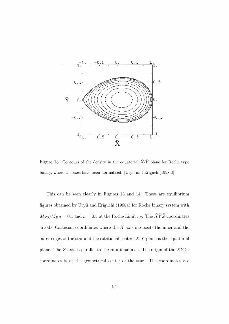
Figure 13: Contours of the density in the equatorial X-Y plane for Roche type

binary, where the axes have been normalised. [Uryu and Eriguchi(1998a)]

This can be seen clearly in Figures 13 and 14. These are equilibrium

figures obtained by Uryu and Eriguchi (1998a) for Roche binary system with

MNS/MBH = 0.1 and n = 0.5 at the Roche Limit rR. The XY Z-coordinates

are the Cartesian coordinates where the X axis intersects the inner and the

outer edges of the star and the rotational center. X-Y plane is the equatorial

plane. The Z axis is parallel to the rotational axis. The origin of the XY Z-

coordinates is at the geometrical center of the star. The coordinates are

95

normalised by

R0 = (Rout −Rin)/2 (150)

where Rout and Rin are distances from the rotational axis to the outermost

and innermost edges of the star respectively. The difference between two

subsequent density contours for each quantity is 1/10 of the difference be-

tween maximum to minimum value.

Figure 14: Contours of the density in the meridional X-Z plane for Roche type

binary, where the axes have been normalised. [Uryu and Eriguchi(1998a)]

96

Figure 16 is the corresponding figures for the IRR-type binary at the

Roche Limit, r = rR, p = 0.1 and n = 0.5. Comparing each of these figures,

Figure 15: Contours of the density in the equatorial plane for IRR-type binary,

with p = 0.1 and n = 0.5. [Uryu and Eriguchi(1998a)]

a difference is detected in the shape, with the Roche-type being more prolate

and the IRR-type less prolate.

97

Figure 16: Contours of the density in the meridional X-Z plane for IRR-type

binary, with p = 0.1 and n = 0.5. [Uryu and Eriguchi(1998a)]

The difference in shape between the Roche-type and IRR type is more

clearly seen in the comparison for the figures in the Y -Z plane for the Roche

type ( Figure 17) and the IRR-type ( Figure 18) binaries.

98

Figure 17: Contours of the density in the meridional Y -Z plane for Roche type

binary, with p = 0.1 and n = 0.5. [Uryu and Eriguchi(1998a)]

99

Figure 18: Contours of the density in the meridional Y -Z plane for the IRR-type

binary, with p = 0.1 and n = 0.5. [Uryu and Eriguchi(1998a)]

100

In a subsequent paper, Uryu and Eriguchi (2000) include the shape of the

surface of the model for the gaseous component of the IRR binary system

with r = rR, p = 0.1 and n = 0.5. We include this figure here as Figure 19 .

Figure 19: Surface shape of the gaseous component of the IRR binary system with

n = 0.5 and MNS/MBH = 0.1 polytropes. [Uryu and Eriguchi(2000)]

101

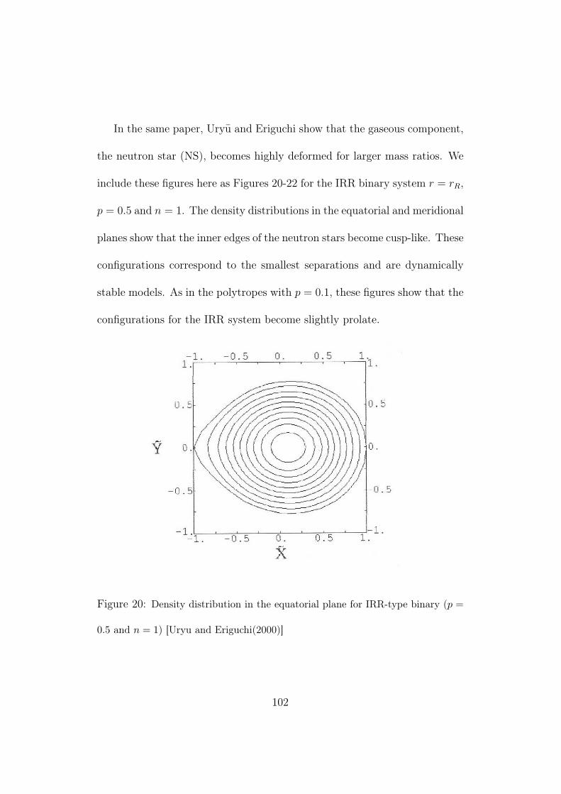
In the same paper, Uryu and Eriguchi show that the gaseous component,

the neutron star (NS), becomes highly deformed for larger mass ratios. We

include these figures here as Figures 20-22 for the IRR binary system r = rR,

p = 0.5 and n = 1. The density distributions in the equatorial and meridional

planes show that the inner edges of the neutron stars become cusp-like. These

configurations correspond to the smallest separations and are dynamically

stable models. As in the polytropes with p = 0.1, these figures show that the

configurations for the IRR system become slightly prolate.

Figure 20: Density distribution in the equatorial plane for IRR-type binary (p =

0.5 and n = 1) [Uryu and Eriguchi(2000)]

102

Figure 21: Density distribution in the meridional X-Z plane for IRR-type binary

(p = 0.5 and n = 1) [Uryu and Eriguchi(2000)]

103

Figure 22: Density distribution in the meridional Y -Z plane for IRR-type binary

(p = 0.5 and n = 1) [Uryu and Eriguchi(2000)]

4.4 Black Hole- Neutron Star Binaries in Full General

Relativity

Most of the attention in the study of compact binaries, has been on dou-

ble binaries : Binary Neutron Stars, (BNS or NSNS), and Binary Black

Holes, (BBH or BHBH). Both fully general realitivistic gravitation as well

as physically realistic equations of state have been included in recent treat-

104

ments of NSNS mergers (Shibata, Tanigichi and Uryu, 2005 and Shibata and

Taniguchi,2006). Progress on the numerical evolution of merging BHBH bi-

naries has been rapid, with Pretorius (2005) performing the stable merger

of two equal mass black holes, through the implementation of generalised

harmonic coordinates. The study of NSBH binaries has enjoyed less atten-

tion, albeit that they are expected to represent a significant proportion of

compact mergers visible in gravity waves and NSBH mergers are predicted to

be one of the most likely progenitors for short gamma-ray bursts (SGRBs).

For the research that has been conducted on NSBH binaries, the majority

has been performed in Newtonian gravity. The scenario based on the tidal

approximation studies may be incorrect as gravitational radiation reaction

and gravititional effects of NS to the orbital motion are ignored.

The reason that research into NSBH binaries has lagged behind those of

double binaries is simply the high costs of computer simulations, together

with the high costs of developing the appropriate computational infrastuc-

ture. This necessitates the development of a framework which admits the

use of approximations, thus dratically reducing the computational resources

needed. Stationary states of NSBH binary systems provide models just prior

to coalescence. Relativistic astrophysicists have tried to solve equilibrium

configurations of highly deformed close binary star systems by devising nu-

105

merical schemes for the binaries. The expected observational data of the GW

detectors will be compared against the theoretical results for the ISCO. These

will provide a large amount of information about the macroscopic quantities

of mass and spin of the neutron star as well as microscopic characters such

as the EOS and the viscosity (Cutler, et al. 1993; Shibata 1997 ; Baumgarte

et al. 1997, 1998a, 1998b ; Bonazzola, Gourgoulhon and Marck 1997).

Simulating coalescing binary systems, requires that initial data be pro-

duced that both satisfy the Einstein constraint equations and are as phys-

ically relevant as possible. The initial configurations are then evolved for-

ward in time. Most of the initial data for coalescing binaries depend on the

quasiequilibrium (QE) hypothesis, which assumes that the objects are on

exact closed circular orbits. Whilst no closed orbits can exist for those sys-

tems in general relativity, this is a good approximation for large separations

(Grandclément 2006). Research into binary neutron stars (BNS) using this

approximation, have been done by Baumgarte et al. 1998a, 1998b; Usui,

Uryu and Eriguchi 2000; Uryu and Y. Eriguchi 2000; Gourgoulhon et al.

2001. The QE approach has also been applied to the binary black hole system

(BBH) by Pfeiffer, Teukolsky and Cook 2000; Gourgoulhon, Grandclément

and Bonazzola 2002; Grandclément, E. Gourgoulhon and S. Bonazzola 2002

and Caudill 2006. Whilst the quasiequilibrium approximation is a good one

106

for large separation, it becomes less accurate as the distance between the

compact objects decrease. Eventually the approximation breaks down neces-

sitating the use of full dynamical simulations. Recently, Bishop et al. (2005),

made a first step in this direction in a relativistic context. Their approach

showed that the initial spurious GW signal resulting from the approxima-

tions in the calculation of the initial data are rapidly radiated away. As a

result, the NSBH relaxes to a quasi-equilibrium state with an approximate

orbital motion of the NS which has been followed only for a small fraction

of an orbit. They have developed and implemented a numerical relativity

code(within the characteristic framework) for evolving a star in close orbit

around a Schwarzschild black hole. The conservative formulation of the hy-

drodynamics, provides procedures for determining initial data. The study

does not take into account variations of the initial matter data, such as the

shape or size of the star, which would occur if tidal distortion were allowed.

A similar approach to Bishop et al., (2005), is used by Sopuerta, Sper-

hake and Laguna, (2006). They treat the problem in full general relativity,

by ’freezing’ the hydrodynamics of their neutron star. For large black hole-

to-neutron star mass ratios the approximation is valid if in addition the

dynamical timescales related with the deformation of the neutron star are

much bigger than the orbital timescales. In their hydro-without-hydro ap-

107

proximation they freeze most of the hydrodynamical degrees of freedom and

evolve only a finite number of them with their attention focussed on the

radiation-reaction effects in the orbit. The reduction of the degrees of free-

dom avoids the use of hyrodynamical computations. In this approximation

scheme, the internal and external motions, which are generally coupled, are

separated. The former motion consists of the evolution of the parameters

describing the deformations of the matter distributions due to the tidal de-

formations, for instance. The latter motion consists of the orbital motion of

a reference point in the matter distribution (a relativistic generalisation to

the Newtonian concept of centre of mass).

First simulations of a head-on collision of a neutron star and a black hole

of comparable mass in full General Relativity have been conducted by Loffler,

Rezzolla, and Ansorg (2006). They do not set any limitations on the mass

ratio between the black hole and the neutron star, nor on the position of the

black hole, whose apparent horizon is entirely contained within the compu-

tational domain. For a prototypical binary system with mass ratio 6, they

find that although a tidal disruption is evident, the neutron star is accreted

promptly and entirely into the black hole. They also discuss a new approach

for obtaining initial data for mixed binary systems and include an extraction

of the gravitational wave signal produced in their study.

108

Taniguchi et al. (2007a, 2007b) have pursued a systematic approach to de-

veloping increasingly realistic models of BHNS binaries in quasiequilibrium

circular orbits. Their first studies (Faber et al. 2006; Baumgarte, Skoge,

and Shapiro 2004; Taniguchi et al. 2005) assumed extreme mass ratios, i.e.

mBH ≫ mNS. From a computational point of view, this is a very natural first

step. However, binaries with comparable masses are much more interesting

from the perspective of ground-based gravitational wave observations and

for the launching of SGRBs. They have extended their results to the case

of comparable-mass BHNS binaries Taniguchi et al. (2006, 2007a, 2007b).

They adopt a polytropic equation of state and focus on irrotational neu-

tron star configurations as well as approximately nonspinning black holes.

In order to ascertain the ISCO they try to locate turning points along both

the binding energy and total angular momentum curves. They also identify

the formation of cusps on the neutron star surface, indicating the onset of

tidal disruption. By comparing critical binary separations for different mass

ratios and neutron star compactions they distinguish those regions of param-

eter space that will lead to a tidal disruption of the neutron star from those

that will result in the plunge into the black hole of a neutron star more or

less intact, albeit distorted by tidal forces. They also estimate the energy

spectrum of the outgoing gravitational radiation emitted during the inspiral

109

phase for these binaries.

Other recent work includes that of Tsokaros and Uryu (2007) and Shibata and

Taniguchi (2007). Tsokaros and Uryu (2007) present a new numerical method

to construct binary black hole - neutron star initial data. The method uses

three spherical coordinate patches. Shibata and Taniguchi (2007) system-

atically perform the merger simulation of black hole-neutron star (BH-NS)

binaries in full general relativity, focusing on the case where the NS is tidally

disrupted. BH-NS binaries in a quasicircular orbit are prepared with initial

conditions in which the BH is modeled by a nonspinning moving puncture.

They investigate the binary for varying mass ratios and separation differ-

ences. They also present gravitational waveforms during the inspiral, tidal

disruption of the NS, and subsequent evolution of the disrupted material.

The amplitude of gravitational waves is found to decrease quickly after the

onset of tidal disruption.

110

5 Observation and Detection

5.1 Population Synthesis

Currently no black hole-neutron star binary systems have been confirmed.

So far, 8 double neutron stars (DNS) have been observed (Stairs 2004).

Over the last three decades, population synthesis studies (Lattimer and

Schramm 1976; Narayan, Piran and Shemi 1991; Tutukov and Yungelson

1993; Lipunov, Postnov and Prokhorov 1997; Portegies Zwart and Yungel-

son 1998; Belczýnski and Bulik 1999; Kalogera et al. 2001) have indicated

that the rate of NSBH mergers is comparable to that of double neutron star

binaries, and is on the order of 10−6 to 10−5 per year per galaxy. However,

there is some controversy about the rates at which NSBH mergers do occur.

Bethe and Brown (1998) argued that NSBH should merge about an order

of magnitude more frequently than DNS, while a recent study by Pfahl et

al. (2005) comes to the conclusion that the number of NSBH systems in the

Galaxy should be below 1 % of the number of double neutron star systems.

In order for NSBH binaries to become both an astronomical and physical

reality, evidence must be obtained that these configurations can be and have

been produced. The current situation is not too dissimilar to what it was

111

with neutron stars, after their theoretical possibilty had been proposed by

in 1934, by Zwicky and Baade in their paper Supernovae and Cosmic Rays.

The first theoretical model was only published in 1939 by Oppenheimer and

Volkoff, whilst the discovery of pulsars by Bell and Hewish took place in

1967. Hulse and Taylor (1975) discovered the first binary pulsar B1913+16

in 1975. This last discovery has, in turn, provided the first evidence for

the existence of gravitational radiation (Taylor and Weisberg 1982). This

DNS has also become valuable in testing general relativity in the strong-field

regime (Taylor and Weisberg 1989).

112

Authors NS + NS NS + BH BH + BH

[yr−1] [yr−1] [yr−1]

Tutukov and Yungelson (1993) 3 × 10−4 2 × 10−5 1 × 10−6

van den Heuvel and Lorimer (1996) 8 × 10−6

Lipunov et al. (1997) 3 × 10−5 2 × 10−6 3 × 10−7

Portegies Zwart and Yungelson (1998) 2 × 10−5 10−6

Bethe and Brown (1998) 10−5 2 × 10−4

Nelemans et al. (2001) 2 × 10−5 4 × 10−6

Voss and Tauris (2003) 2 × 10−6 6 × 10−7 10−5

O’Shaughnessy et al. (2005) 7 × 10−6 1 × 10−6 1 × 10−6

de Freitas Pacheco et al. (2006) 2 × 10−5

Table 4: Population synthesis calculations of merger rates of compact binaries

by various groups.

113

5.2 Gravitational Waves

According to the theory of general relativity, as formulated by Einstein (1916,

1918), the force of gravity is due to curvature of spacetime caused by the

presence of massive objects. The curvature is more pronounced the greater

the mass of the object, which in turn increases the gravity. The motion of

massive objects in spacetime produces changes to the curvature and if this

motion occurs in a paticular way, ripples in the curvature of spacetime can

be produced, which are referred to as gravitational waves. These waves are

produced for accelerating masses, provided that the motion is not spheri-

cally or cylindrically symmetrical. The finite speed of light and gravitational

influence is crucial to the existence of gravitational radiation. Mathemati-

cally, for gravitational radiation to occur, the second time derivative of the

quadrupole moment (or the l-th time derivative of the l-th multipole mo-

ment) of the stress-energy tensor (of an isolated system) must be non-zero.

For this reason we do not expect gravitational radiation from an isolated non-

spinning object moving at constant speed nor from a spherical star pulsating

spherically. However, two masses orbiting each other will produce gravita-

tional radiation. From any standard text on gravitation such as (Misner,

Thorne and Wheeler 1973), the quadrupole approximation to the Einstein

114

field equations give :

h ≈ (G/c4)Q/r (151)

where Q is the second time derivative of the source’s quadrupole moment

and r is the distance of the source from the Earth. We also see from (Misner,

Thorne and Wheeler 1973) that : The corresponding power loss for two

orbiting masses M1 and M2 with separation R is given by

P =dE

dt= −32G4

πc5(M1M2)

2 (M1 +M2)

R5(152)

For the Earth-Sun system, this power loss is only about 300 watts. Compare

this with the electromagnetic radiation of the sun of about 3.86× 1026 watts

or to the kinetic energy of the Earth orbiting the Sun of about 2.7 × 1033

joules. The scenario is very different for close compact binaries such as a

NSBH binary.

Electromagnetic radiation forms the basis for much of our present under-

standing of the universe. Gravitational waves are set to revolutionise that

understanding in that they are significantly different from electromagnetic

waves. The following table compares them in an astronomical context.

115

Electromagnetic Waves Gravitational Waves

typical sources of electromagnetic

waves are stellar athmospheres, ac-

cretion discs and clouds of interstel-

lar dust, none of which emit signifi-

cant gravitational waves.

sources are collisions and mergers

of black holes and other compact

objects and emit very little elec-

tromagnetic radiation; the cores of

supernovae which are hidden from

electromagnetic view by dense lay-

ers of surrounding stellar gas.

propagate through spacetime as os-

cillating fields of coexisting electric

and magnetic fields.

propagate as oscillations of the ’fab-

ric’ of spacetime itself.

are almost always incoherent super-

positions of emission from individ-

ual electrons, atoms, or molecules.

produced by coherent, bulk motions

of huge amounts of mass-energy - ei-

ther material mass, or the energy of

vibrating, nonlinear spacetime cur-

vature.

116

wavelengths of electromagnetic

waves are small compared to

their sources (gas clouds, stellar

atmospheres, accretion disks, ...),

so from the waves we can make

pictures of the sources.

wavelengths of cosmic gravitational

waves are comparable to or larger

than their coherent, bulk-moving

sources, so we cannot make pictures

from them. Instead, the gravita-

tional waves are like sound; they

carry, in two independent wave-

forms, a stereophonic, symphony-

like description of their sources.

easily absorbed, scattered, and dis-

persed by matter.

travel nearly unscathed through all

forms and amounts of intervening

matter.

frequencies range from about 107

Hz upwards by around 20 orders of

magnitude.

frequencies should range from

around 104 Hz downwards by about

20 orders of magnitude.

information brought to us by elec-

tromagnetic waves show us the ther-

modynamic state of optically thin

concentrations of matter.

gravitational waves will show us de-

tails of the bulk motion of dense

concentrations of energy.

117

The frequency range of the gravitational waves may be broken into four

frequency bands :

• The Extremely Low Frequency Band (ELF)

range : 10−15 to 10−18 Hz.

The measured anisotropy of the cosmic microwave background radia-

tion places strong limits on gravitational wave strengths and may, in

fact, have detected waves.

The only waves expected in this band are relics of the big bang.

• The Very Low Frequency Band (VLF).

range : 10−7 to 10−9 Hz.

The only expected strong sources in this band are processes in the very

early universe such as the big bang, phase transitions of the vacuum

states of quantum fields, and vibrating or colliding defects in the struc-

ture of spacetime, such as monopoles, cosmic strings, domain walls,

textures, and combinations thereof.

• The Low-Frequency Band (LF).

range : 10−4 to 1 Hz. Joseph Taylor and others have achieved remark-

able gravity-wave sensitivities by the timing of millisecond pulsars.

118

The Laser Interferometer Space Antenna, LISA will operate in this fre-

quency range.

This is the band of massive black holes (M 1000 to 108M.) in the dis-

tant universe, and of other hypothetical massive exotic objects (naked

singularities, soliton stars), as well of as binary stars (ordinary, white

dwarf, neutron star, and black hole)

• The High-Frequency Band (HF).

range : 1 to 104 Hz.

Earth-based gravitational-wave detectors such as LIGO, VIRGO and

TAMA operate in this frequency range. This is the band of stellar-mass

black holes (M 1 to 1000M. and of other conceivable stellar-mass exotic

objects (naked singularities and boson stars) in the distant universe,

as well as of supernovae, pulsars, and coalescing and colliding neutron

stars. Early universe processes should also have produced waves at

these frequencies, as in the ELF, VLF, and LF bands.

5.3 Gravitational Wave Detection by Interferometers

From general relativity, a gravitational wave has two linear polarisations.

These polarisations each have an associated gravitational-wave field which

119

oscillates in time and propagates at the speed of light. As each wave passes

through any object it produces tidal forces. For objects that are compar-

itively small in relation to the wavelength of these waves, the forces have

quadrapolar patterns relative to the object’s center. These patterns are

shown in Figure 12.

Figure 23: The lines of force associated with the two polarizations of a gravita-

tional wave. [From Ref. Abramovici et. al. (1992)]

From the force patterns characterised by the orientation of the axis, the

polaristaions have derived the names ’plus’(+) and ’cross’ (×). Each of the

gravitational wave fields are in turn named h+ and h×.

The Weber bar, a large, solid piece of metal with electronics attached to

detect any vibrations was the first type of gravitational wave detector. Pass-

ing gravitational waves “ring up” the bar at its resonant frequency, which

would basically amplify the wave naturally. Nearby supernova may be strong

120

enough to be seen without resonant amplification. Modern forms of the We-

ber bar are still operated, cryogenically cooled, with superconducting quan-

tum interference devices to detect the motion. However they are not sensitive

enough to detect anything but extremely powerful gravitational waves.

Currently, gravitational wave detectors consist of a laser interferometer

with four masses hanging from vibration-isolated supports with an optical

system to monitor the separations between the masses. Figure 12 illustrates

such a detection sytem.

Figure 24: Schematic diagram of a laser interferometer gravitational wave detector.

[From Ref. Abramovici et. al. (1992)]

The device consists of two long arms at right angles to each other meeting

each other in such a manner as to form an ’L shape’. A mass is placed at

each end of the long arms of the ’L shape’, whilst two masses are placed

121

near each other at the corner of the ’L’. The arm lengths are approximately

equal, with L1 ≃ L2 = L. As a gravitational wave (with high frequencies in

comparison to the masses’ ∼ 1Hz pendulum frequency) passes through the

detector, the masses are pushed back and forth relative to each other. This

results in a change in the arm-length difference, i.e. ∆L ≡ L1−L2. Through

laser interferometry that change is monitored. The variations in the output

of the photodiode (the output of the interferometer) is directly proportional

to ∆L. If the gravitaional waves are arriving from above or below the device

and the axes of the + polarisation coincide with the arm’s directions, then it

is the waves’ + polarisation that will drive the massses. We may then write

:

∆L(t)

L= h+(t). (153)

In general, though, it is more likely that the interferometer’s output is a

linear combination of the two wave fields :

∆L(t)

L= F+h+(t) + F×h× ≡ h(t). (154)

h(t) is referred to as the gravitational wave-strain acting on the detector.

Reliable detection of gravitational waves requires the operation of at least

two detectors in coincidence - if the signals coincide with those of a distant

detector, local perturbations can be ruled out. In order to obtain the full

information about the gravitational waves (source position, polarization),

122

data from at least four detectors have to be compared. For a NSBH bi-

nary’s inspiral and coalescence, two gravitational waves are produced, one

for each polarisation. The waveform can be divided into three parts. The

first, the inspiral waveform is emitted before tidal distortions become no-

ticeable; the second, the coalesence waveform is emitted during distortion,

disruption and/or merger; and the third, the ringdown waveform is due to

the excitation of quasi-normal modes of the black hole.

5.4 Currently Operational Ground-based Laser Inter-

ferometers

• LIGO

The Laser Interferometer Gravitational-Wave Observatory (LIGO) is

a US Project consisting of two detectors (4km). LIGO operates two

gravitational wave observatories in unison: the LIGO Livingston Ob-

servatory in Livingston, Louisiana and the LIGO Hanford Observatory,

on the Hanford Nuclear Reservation located near Richland, Washing-

ton. These sites are separated by 3,002 kilometers. Since gravitational

waves are expected to travel at the speed of light, this distance corre-

sponds to a difference in gravitational wave arrival times of up to ten

123

milliseconds. Using triangulation, the difference in arrival times can

restrict the location of the source of the wave in the sky. Each obser-

vatory supports an L-shaped ultra high vacuum system, measuring 4

kilometers on each side. Up to five interferometers can be set up in

each vacuum system.

• VIRGO

The VIRGO collaboration was set up between Italian and French re-

search teams. The Virgo detector for gravitational waves consists

mainly in a Michelson laser interferometer made of two orthogonal arms

being each 3 kilometers long. Multiple reflections between mirrors lo-

cated at the extremities of each arm extend the effective optical length

of each arm up to 120 kilometers. The frequency range of Virgo extends

from 10 to 6,000 Hz. This range as well as the very high sensitivity

should allow detection of gravitational radiation produced by super-

novae and coalescence of binary systems in the milky way and in outer

galaxies, for instance from the Virgo cluster.

• GEO 600

Of all the large interferometric gravitational-wave detectors, the Ger-

man/British project GEO600 is the only one which uses dual recycling.

GEO600, with an interferometric gravitational-wave detector of arm

124

length 600 m, is in northern Germany close to Hannover. GEO600 in-

corporates an externally modulated fourfold delay-line Michelson inter-

ferometer giving a round-trip optical length of 2400 m. Power recycling

increases the light power inside the interferometer to a level of about 10

kW. The use of both power and signal recycling will yield a sensitivity of

the same order of magnitude as the first stages of the other large-scale

gravitational-wave detectors LIGO and VIRGO. High signal recycling

factors allow the sensitivity to be increased at a chosen frequency while

reducing the bandwidth of the detector. This gives an advantage over

broad-band detectors in detecting narrow-band periodic sources such

as pulsars. The 25 cm diameter mirrors will be suspended as double

pendulums from a platform supported by vibration-reduction systems.

The passive filtering properties of this system sufficiently reduce the

seismic noise in the frequency range of interest, i.e. 50 - 1000 Hz.

Between 2002 and 2006 GEO600 participated in several data runs in

coincidence with the LIGO detectors and is now gradually approaching

design sensitivity.

• TAMA 300

The Japanese project has an interferometric gravitational-wave detec-

tor of arm length 300 m. TAMA operations began with much success

125

in 1999, soon achieving world’s-best sensitivity and the longest accu-

mulated data set during its runs in 2000 and 2001. With the start of

the LIGO science run in 2002, TAMA aggressively joined the effort,

helping to forge the international collaboration of coincidence analysis

by scheduling operation time and sharing analysis methods and data.

5.5 Future Plans for Gravitational Wave Detectors

• Advanced LIGO

As the initial LIGO interferometers start to put new limits on gravita-

tional wave signals, the LIGO Lab, the LIGO Scientific Collaboration,

and international partners are proposing Advanced LIGO to improve

the sensitivity by more than a factor of 10. This new detector, to be

installed at the LIGO Observatories, will replace the present detector

once it has reached its goal of a year of observation, and will transform

gravitational wave science into a real observational tool. It is antic-

ipated that this new instrument will see gravitational wave sources

possibly as often as daily, with excellent signal strengths, allowing de-

tails of the waveforms to be read off and compared with theories of

neutron stars, black holes, and other highly relativistic objects. The

126

improvement of sensitivity will allow the one-year planned observation

time of initial LIGO to be equaled in just several hours.

The change of more than a factor of 10 in sensitivity comes also with

a change in the bandwidth of high sensitivity, and the ability to tune

the instrument for specific astrophysical sources. This will allow Ad-

vanced LIGO to look at the inspiral, coalescence, and ringdown of pairs

of black holes up to 50 solar masses, and to pinpoint periodic signals

from the many known pulsars which radiate in the range from 500-

1000 Hertz. A program of testing and practice installation will allow

the new detectors to be brought on-line with a minimum of interruption

in observation. The design of the instrument has come from scientists

throughout the 40-institution, 400-person LIGO Scientific Collabora-

tion, an international group which carries out both instrument devel-

opment and scientific data analysis. Observations will start in 2013.

• LCGT

The Large-scale Cryogenic Gravitational-wave Telescope, LCGT, is the

next generation interferometer now under proposal in Japan. This

powerful new instrument has a sensitivity comparable to the Advanced

LIGO design and a far-reaching sky coverage complementary to that

of other gravitational-wave detectors. The unique design of LCGT

127

is its use of a cryogenic system to suppress thermal noise. Sapphire

was chosen for the substrate material because of its optical thermal

conductivity and measured high Q values at low temperatures.

• LISA

As the first dedicated space-based gravitational wave observatory, LISA

will detect waves generated by binaries within our Galaxy, the Milky

Way, and by massive black holes in distant galaxies. Although gravi-

tational wave searches in space have previously been made, they were

conducted for short periods by planetary missions that had other pri-

mary science objectives. Some current missions are using microwave

Doppler tracking to search for gravitational waves. However, LISA

will use an advanced system of laser interferometry for detecting and

measuring them. And, LISA will directly detect the existence of grav-

itational waves, rather than inferring it from the motion of celestial

bodies, as has been done previously. Additionally, LISA will make its

observations in a low-frequency band that ground-based detectors can’t

achieve. Note that this difference in frequency bands makes LISA and

ground detectors complementary rather than competitive. This range

of frequencies is similar to the various types of electromagnetic wave-

lengths detected in astronomy, such as ultraviolet and infrared. Each

128

provides different information. In space, LISA won’t be affected by

the environmental noise that affects ground detectors on Earth’s sur-

face. Due to earthquakes and other vibrations, ground detectors can

only make observations at frequencies above 1 hertz. However, other

environmental factors will impact LISA. Such factors include the drift

of the spacecraft, charging of the test masses, and buffeting by the so-

lar wind. Making these small disturbances negligible is a technological

challenge of the mission. Meeting this challenge will help to ensure the

detection of gravitational waves. LISA is expected to be operational

by 2015.

5.6 Gamma-Ray Bursts

The first gamma-ray burst(GRB) was detected on the 2nd of July 1967 by

the US Vela nuclear test detection satellites. The discovery of GRBs was con-

firmed by many later space missions, including Apollo and the Soviet Venera

probes. Many speculative theories about these events were presented, most of

which involved nearby Galactic sources. However, there were no major new

advancements until the launch in 1991 of the Compton Gamma Ray Obser-

vatory and its Burst and Transient Source Explorer (BATSE) instrument, an

129

extremely sensitive gamma-ray detector. Among the crucial pieces of infor-

mation provided by this instrument were that gamma-ray bursts are isotropic

(that is, not biased towards any particular direction on the sky such as the

Galactic plane or Galactic center), ruling out nearly all Galactic origins; and

that they fall into two apparently distinct categories, short-duration, hard-

spectrum bursts (“short bursts”) and long-duration, soft-spectrum bursts

(“long bursts”). Short bursts are typically less than two seconds in dura-

tion and are dominated by higher-energy photons; long bursts are typically

more than two seconds in duration and dominated by lower-energy photons.

The separation is not absolute and the populations do overlap observation-

ally, but the distinction suggested two different classes of progenitors. There

is now almost universal agreement in the astrophysics community that the

long-duration bursts are associated with the deaths of massive stars in a

specific kind of supernova-like event commonly referred to as a collapsar.

While the astrophysical community has yet to settle on a single, uni-

versally favored model for the progenitors of the short-duration events, the

general preferred model is the merger of two compact objects as a result of

gravitational inspiral: two neutron stars, or a neutron star and a black hole.

A revolution in GRB astronomy is in progress today, largely as a result of

130

the successful launch of NASA’s Swift satellite, which combines a sensitive

gamma-ray detector with the ability to slew on-board X-ray and optical

telescopes to the direction of a new burst in under one minute. Among

the discoveries so far are the first discoveries of short burst afterglows and

vast amounts of data on the behavior of GRB afterglows at early times in

their evolution, even before the GRB itself (that is, the gamma-ray emission)

has stopped, and the discovery of huge X-ray flares appearing from minutes

to days after the end of the GRB. Additional discoveries are being made

constantly, and as such, the study of GRBs is one of the most dynamic in all

of astrophysics.

131

6 Conclusions

It has been nearly a century since the theory of relativity was first postu-

lated by Einstein. Even before this theory was fully formulated (Einstein

1916, 1918), it became clear to Einstein and others that the theory would

have to predict gravitational waves. Almost immediately after formulating

the General Theory of Relativity, Einstein worked out the basic properties

of those waves. Detection of these waves has been elusive, primarily due to

the difficulty in creating the technology to do so. Over the next few years,

the sensitivity of terrestrial-based detectors will reach levels of expected de-

tection. Close binary systems such as the neutron star black hole binary, are

considered as the primary targets for the forthcoming field of gravitational

wave astronomy. For compact objects such as a neutron star and a black hole

in a binary configuration, the emission of gravitational waves completely con-

trols the orbital evolution, which eventually leads to the coalescence of the

components. It is extremely difficult to complete analytical calculations of

these gravitational waves and so numerical investigations remain the only

viable option in the final stages of evolution. This is in itself is a challenging

task. For a neutron star in the vicinity of a black hole, gravitational waves

are generated due to the quadrupole moment of the star-black hole system

132

changing in time. By computing the stellar shape and structure along its mo-

tion due to the time-varying deformation, we can construct quasi-statically

evolutionary sequences of the inspiraling neutron star. In so doing we can at-

tempt to evolve the star until the last few moments before merger, where the

nonlinear character of the gravitational and tidal effects become important.

This will enable us to prepare initial conditions for numerical simulations of

the merging of the binary neutron star black hole in full general relativity.

Apart from this, the problem of tidal deformation in itself is an interesting

problem. Analytical solutions exist for various binary configurations mainly

in Newtonian gravity. Providing an analytical solution for the tidal deforma-

tion of a neutron star in the vicinity of a black hole, fully taking into account

general relativistic effects, is unlikely to occur in the near future, if at all.

133

Appendices

A The Interior Potential of Homoeiodal Shells

A homoeoid is a shell bounded by two similar concentric ellipsoids in which

strata of equal density are also ellipsoids that are concentric with and similar

to the bounding ellipsoids.

We first state a theorem due to Newton and its corollary :

Theorem 1 (Newton’s Theorem) The attraction at any internal point

of a homogeneous homoeoid is zero.

Corollary The theorem is true for any heterogeneous homoeoid in which

the strata of equal density are ellipsoids concentric with and similar to the

bounding ellipsoids.

The following theorem also follows from Newton’s Theorem.

Theorem 2 The constant potential inside a homogeneous homoeoidal shell

enclosed between the ellipsoids with the semi-axes ai and qai, where

134

a1 ≤ a2 ≤ a3 and q < 1 is given by

B =1

2Gρ(1 − q2)

∫

S

r2dω (155)

where r is the radius vector drawn from the centre to a point on the surface

(S) of the outer bounding ellipsoid defined by

3∑

i=1

(x2

i

a2i

) = 1 (156)

Proof. From Newton’s Theorem, the potential is constant throughout the

interior and equal to its value at the centre.

Now, consider an elementary cone of solid angle dω, with its vertex at the

centre, the contribution to B by the frustrum of the cone intercepted by the

homoeoid is

∫ r2

r1

Gρrdωdr = Gρdω

[

r2

2

]r2

r1

=1

2Gρ(r2

2 − r2

1)dw (157)

where, r22 and r2

1 are the radii of the outer and inner surfaces of the ho-

moeoid in the direction of the cone.

Now, r1 = qr2

135

So, B =∫

S1

2Gρ(r2

2 − q2r22)dω

Hence,

B =1

2Gρ(1 − q2)

∫

S

r2dω (158)

which is the constant potential inside a homogeneous homoeoidal shell en-

closed between the ellipsoids with the semi-axes ai and qai.

The mass of our homoeiodal shell is given by :

M =4

3πa1a2a3(1 − q3) × ρ (159)

giving

ρ =M

4

3πa1a2a3

.1

(1 − q3)(160)

hence

B =1

2GM

4

3πa1a2a3

.1 − q2

(1 − q3)

∫

s

r2dω (161)

Now,

limq→1

1 − q2

(1 − q3)= limq→1

(1 − q2)′

(1 − q3)′

= limq→1

−2q

−3q2

=2

3

136

So, for fixed M , as q → 1, we get

B =GM

4πa1a2a3

∫

s

r2dω (162)

Now,

x1 = r sin θ cosχ (163)

x2 = r sin θ sinχ (164)

x3 = r cos θ (165)

But,

1 =3∑

i=1

(

x2i

a2i

)

=x2

1

a21

+x2

2

a22

+x2

3

a23

=r2 cos2 θ

a23 + r2 sin2 θ

(

cos2 χ

a21

+sin2 χ

a22

)

∴1

r2=

cos2 θ

a23

+ sin2 θ

(

cos2 χ

a21

+sin2 χ

a22

)

(166)

(167)

We make the substitution : t = tanχ

137

with,

dt = sec2 χdχ

t2 =sin2 χ

cos2 χ

dχ = cos2 χdt

We can then write :

dχ[

cos2 θa2

3

+ sin2 θ(

cos2 χa2

1

+ sin2 χa2

2

)]−1

= dt[

cos2 θcos2 χ.a2

3

+ sin2 θ(

1

a2

1

+ sin2 χcos2 χ.a2

2

)]−1

= dt[

(sin2 θ + cos2 θ) cos2 θcos2 χ.a2

3

+(

sin2 θa2

1

+ t2. sin2 θ

a2

2

)]−1

= dt[

sin2 θa2

1

+ cos2 θa2

3

+ t2(

sin2 θa2

2

+ cos2 θa2

3

)]−1

138

Now, with 0 ≤ χ ≤ π and 0 ≤ θ ≤ π , we have :

∫

S

r2dω = 8

∫ π2

0

∫ π2

0

sin θdθdχ

cos2 θa2

3

+ sin2 θ(

cos2 χa2

1

+ sin2 χa2

1

) (168)

Making the substitution, t = tanχ, we get by symmetry:

∫

S

r2dω = 8

∫ 1

2

0

∫ π2

0

dθ sin θdt

[

sin2 θa2

1

+ cos2 θa2

3

+ t2(

sin2 θa2

2

+ cos2 θa2

3

)] (169)

But,

∫

∞

0

dx

a2 + x2=

π

2a

so,

∫

∞

0

dx

a2 + b2x2=

π

2ab

∴

∫

S

r2dω = 4π

∫ π2

0

sin θdθ[

(

sin2 θa2

1

) 1

2

+ cos2 θa2

3

×(

sin2 θa2

2

+ cos2 θa2

3

) 1

2

] (170)

Then, multiplying the RHS by( 1

cos2 θ)

( 1

cos2 θ), we get :

139

∫

S

r2dω = 4π

∫ π2

0

(

1

cos2 θ

)

sin θdθ[

(a1a3)−1 (tan2 θa23 + a2

1)1

2 × (a2a3)−1 (tan2 θa23 + a2

2)1

2

]

(171)

Now, we take the transformation :

u = a2

3 tan2 θ

with,

du = 2a2

3 tan θ sec2 θdθ

= 2a2

3 sin θ sec3 θdθ

Hence,

∫

S

r2dω = 2πa1a2

∫

du[

sec θ.(

a2

1 + u) 1

2 +(

a2

2 + u) 1

2

)−1

(172)

Now,

sec θ =(

1 + tan2 θ) 1

2

140

a3 sec θ =(

a2

3 + u) 1

2

Then,

∫

S

r2dω = 2πa1a2a3

∫

∞

0

du[

(

a2

1 + u) 1

2 ×(

a2

2 + u) 1

2 ×(

a2

3 + u) 1

2

]−1

= 2πa1a2a3

∫

∞

0

du

∆(173)

where,

∆2 =[(

a2

1 + u) (

a2

2 + u) (

a2

3 + u)]

(174)

or∫

S

r2dω = 2πL (175)

with

L = a1a2a3

∫

∞

0

du

∆(176)

Now, we introduce li(i = 1, 2, 3), which are the direction cosines of the radius

vector r joining the centre of the ellipsoid to a point on its surface, with :

3∑

i=1

l2i = 1 (177)

141

li = cosαi (178)

=xi − x′id

(179)

d =

[

3∑

i=1

(xi − x′i)2

]1

2

(180)

Next we consider,∫

Sr2l2i dω.

Taking i = 3 first, we get :

∫

S

r2l23dω =

∫

S

r2 cos2 θdω

= 2πa1a2a3

∫

∞

0

cos2 θdω

∆

But,

cos2 θ =1

sec2 θ=

(

1 + tan2 θ)−1

= a2

3

(

a2

3 + u)−1

So,

∫

S

r2l23dω = 2πa1a2a3

∫

∞

0

a23du

∆ (a23 + u)

= 2πa2

3A3 (181)

142

where

A3 = a1a2a3

∫

∞

0

du

∆ (a23 + u)

(182)

By symmetry we can generalise.

∴

∫

S

r2l2i dω = 2πa2

iAi (183)

with

Ai = a1a2a3

∫

∞

0

du

∆ (a2i + u)

(184)

But,

∫

S

r2dω =∑

3

i=1

∫

Sr2l2i dω = 2πL

∴

3∑

i=1

a2

iAi = L (185)

Now,

∂L

∂a3

=∂

∂a3

[

a1a2a3

∫

∞

0

du

∆

]

143

= a1a2

∫

∞

0

du

∆+ a1a2a3

[

∂

∂a3

∫

∞

0

du

∆

]

(186)

But,

∆ =[

(

a2

1 + u) 1

2

(

a2

2 + u) 1

2

(

a2

3 + u) 1

2

]

∴∂

∂a3

∫

∞

0

du

∆=

∫

∞

0

du∂

∂a3

[

(

a2

1 + u)−

1

2

(

a2

2 + u)−

1

2

(

a2

3 + u)−

1

2

]

=

∫

∞

0

du(

a2

1 + u)−

1

2

(

a2

2 + u)−

1

2 (−1

2)(

a2

3 + u)−

3

2 (2a3)

(187)

Thus,

∂L

∂a3

= a1a2

∫

∞

0

du

∆− a1a2a

2

3

∫

∞

0

du

∆ (a23 + u)

= a1a2

∫

∞

0

du

∆− a3A3

(188)

144

We can then write

A3 = − 1

a3

∂L

∂a3

+a1a2

a3

∫

∞

0

du

∆

= − 1

a3

∂L

∂a3

+L

a23

(189)

(190)

This can be generalised to :

Ai =L

a2i

− 1

ai

∂L

∂ai

(191)

So,3∑

i=1

1

(a2i + u)

=2

∆

d∆

du(192)

We have

3∑

i=1

Ai =3∑

i=1

(

a1a2a3

∫

∞

0

du

∆ (a2i + u)

)

= 2a1a2a3

∫

∞

0

d∆

∆2

145

=

[−2a1a2a3

∆

]∞

0

But we can write

∆ = a1a2a3

[(

1 +u

a21

)(

1 +u

a22

)(

1 +u

a23

)] 1

2

Since ua2

1

≥ 0 we have ∆min = a1a2a3. Then,

[−2a1a2a3

∆

]∞

0

=

[

0 − −2a1a2a3

∆

]

= 2 (193)

i.e.3∑

i=1

Ai = 2 (194)

we have

∫

S

r2dω = 2πL

Differentiating w.r.t. ai, we get

∫

s

r

(

∂r

∂ai

)

dω = π

(

∂L

∂ai

)

(195)

146

Now,

1

r2=

cos2 θ

a23

+ sin2 θ

(

cos2 χ

a21

+sin2 χ

a21

)

=l23a2

3

+l21a2

1

+l22a2

2

∴1

r2=

3∑

j

=l2ja2

j

(196)

Differentiating w.r.t ai gives

− 2

r3

(

∂r

∂ai

)

= −2l2ia2

i

∴

(

∂r

∂ai

)

=

(

1

a3i

)

r3l2i (197)

Substituting

∫

S

(

1

a3i

)

r4l2i dω = π

(

∂L

∂ai

)

∴

∫

S

r4l2i dω = πa3

i

(

∂L

∂ai

)

(198)

147

The standard incomplete integrals are

for the first kind

E (ψ, χ) =

∫ χ

0

(

1 − sin2 ψ sin2 χ) 1

2 dχ (199)

and for the second kind

F (ψ, χ) =

∫ χ

0

(

1 − sin2 ψ sin2 χ)−

1

2 (200)

with the definitions :

sinψ =

(

a21 − a2

2

a21 − a2

3

)1

2

(201)

cosχ =a3

a1

=(

1 − e2) 1

2 (202)

where e =(

1 − a2

3

a2

1

) 1

2

148

We can also write :

cosψ =

(

a22 − a2

3

a21 − a2

3

)1

2

(203)

and

sinχ =

(

1 − a23

a21

)1

2

= e (204)

Now,

A1 =2a2a3

a21 sin3 χ sin2 ψ

[F (ψ, χ) − E (ψ, χ)] (205)

A2 =2a2a3

a21 sin3 χ sin2 ψ cos2 ψ

[

E (ψ, χ) − F (ψ, χ) cos2 ψ − a3

a2

sin2 ψ sinχ

]

(206)

A3 =2a2a3

a21 sin3 χ cos2 ψ

[

a2

a3

sinχ− E (ψ, χ)

]

(207)

For the special; case a1 = a2 > a3, we have A1 = A2

149

i.e.

(F − E) =

(

1

cos2 ψ

)[

E − F cos2 ψ − a3

a1

sin2 ψ sinχ

]

(208)

⇐⇒ cos2 ψ (F − E) =

[

E(

cos2 ψ + sin2 ψ)

− F cos2 ψ − a3

a1

sin2 ψ

]

= − (F − E) cos2 ψ +[

E −(

1 − e2) 1

2 e]

sin2 ψ

⇐⇒ 2 cos2 ψ (F − E) = sin2 ψ[

E −(

1 − e2) 1

2 e]

∴ (F − E) =

(

1

2

)

sin2 ψ

cos2 ψ

[

E −(

1 − e2) 1

2 e]

(209)

Hence,

A1 =(a3/a1)

sin3 χ

(

1

cos2 ψ

)

[

E −(

1 − e2) 1

2 e]

=(1 − e2)

1

2

e3.

(

1

cos2 ψ

)

[

E −(

1 − e2) 1

2 e]

150

∴ A1 =

[

E.(1 − e2)

1

2

e3− (1 − e2)

e2

]

(

1

cos2 ψ

)

(210)

We next wish to find the potential of a homogeneous ellipsoid at an interior

point. We first construct an elementary cone of solid angle dω with its vertex

at xi The contribution to the potential at xi by the matter included between

the generators of the cone is given by :

dB = 1

2Gρ (R2

1 +R22) dω

where R1 and R2 are the heights of the two half-cones diverging from xi.

Integrating over all solid angles, noting that each elementary cone will be

counted twice, we get :

B =1

4Gρ

∫

(

R2

1 +R2

2

)

dw (211)

If the apex of the cone is at xi then the axis of the cone intersects the ellipsoid

at :

151

xi + liR1 and xi + liR2

where li are the direction cosines of the radius vector r , drawn from the

centre of the ellipsoid parallel to the elementary cone considered.

Since these points lie on the ellipsoid, it is clear that R1 and R2 are the

roots of the equation :3∑

i=1

(

xi + liR

ai

)2

= 1 (212)

i.e. R2∑

3

i=1

l2ia2

i

+ 2R∑

3

i=1

xilia2

i

+(

∑

3

i=1

x2

i

a2

i

− 1)

= 0

so, we get on multiplying by r2 :

aR2 + bR + c = 0 (213)

where we have written :

a = 1

b = 2r2

3∑

i=1

xilia2

i

c = r2

(

3∑

i=1

x2i

a2i

− 1

)

152

The roots of this equation are R1 and R2.

So,

(R1 +R2) = − b

a

= −b

= −2r2

(

3∑

i=1

xilia2

i

− 1

)

substituting for each of the roots in the quadratic equation above gives :

R2

1 + bR1 + c = 0

R2

2 + bR2 + c = 0

Adding we get :

R2

1 +R2

2 + b (R1 +R2) + 2c = 0

Substituting for (R1 +R2):

(

R2

1 +R2

2

)

− b2 + 2c = 0

∴ R2

1 +R2

2 = b2 − 2c

= 4r4

(

3∑

i=1

xilia2

i

)2

+ 2r2

(

1 −3∑

i=1

x2i

a2i

)

153

Then, we can write :

B =1

2Gρ

∫

s

2r4

(

3∑

i=1

xilia2

i

)2

+ r2

(

1 −3∑

i=1

x2i

a2i

)

dω

Now,∫

r2dω = 2πL

and∫

r4l2i dω = πa3i

∂L∂ai

So,

B =1

2Gρ

∫

s

3∑

i=1

[

(

2r4l2i)

(

x2i

a4i

)

+ r2 − r2

a2i

x2

i

]

=1

2Gρ

3∑

i=1

[(

πa3∂L

∂ai

)(

2x2i

a4i

)

+ (2πL) −(

2πL

a2i

)

x2

i

]

= πGρ3∑

i=1

[

x2

i

(

1

ai

∂L

∂ai

− L

a2i

)]

+ L

But Ai = La2

i

− 1

ai

(

∂L∂ai

)

So, B = πGρ[

L−∑

3

i=1Aix

2i

]

Now by definition,

154

Wij =∫

vρxi

∂B∂xjdx

We have

∂B

∂xj

=∂

∂xj

[

πGρ

(

L−3∑

l=1

Alx2

l

)]

(214)

= πGρ(−2)3∑

j=1

Alxlδlj (215)

= −2πGρ3∑

j=1

Ajxj (216)

Then,

WπGρ

= −2∫

vρ∑

3

j=1Ajxjdx

But,

Iij =∫

vρxixjdx

Consequently,

Wij

πGρ= −2AiIij (217)

155

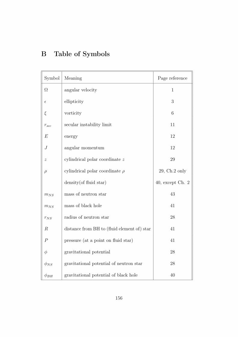
B Table of Symbols

Symbol Meaning Page reference

Ω angular velocity 1

ǫ ellipticity 3

ξ vorticity 6

rsec secular instability limit 11

E energy 12

J angular momentum 12

z cylindrical polar coordinate z 29

ρ cylindrical polar coordinate ρ 29, Ch.2 only

density(of fluid star) 40, except Ch. 2

mNS mass of neutron star 43

mNS mass of black hole 41

rNS radius of neutron star 28

R distance from BH to (fluid element of) star 41

P pressure (at a point on fluid star) 41

φ gravitational potential 28

φNS gravitational potential of neutron star 28

φBH gravitational potential of black hole 40

156

Symbol Meaning Page reference

x position vector of fluid element 41

B gravitational potential 41

W potential energy associated with the grav-

itational potential energy

45

u velocity of fluid element 41

I moment of inertia 44

I kinetic energy of system 44

p mass ratio p = mNS

mBH31

Q mass ratio Q = 1

p= mBH

mNS31

q ratio of radii q = r1

r2

135

ai semi-axes of ellipsoid 134

ω solid angle dω of an elementary cone with

its vertex at the centre

135

r radius of body 6

G Universal Gravitational Constant 29

zc Critical radius ??

157

C Abbreviations Used

Abbreviation Meaning

BBH Binary Black Hole

BH Black Hole

BHNS Black Hole - Neutron Star

BNS Binary Neutron Star

DNS Double Neutron Star

ELF Extremely Low Frequency (Band)

EOS Equation of State

GR General Relativity

GRB Gamma-Ray Bursts

GW Gravitational Wave

HF High-Frequency (Band)

ISCO Innermost Stable Circular Orbit

LF Low-Frequency (Band)

LIGO Laser Interferometer Gravitational Wave Observatory

LISA Laser Interferometer Space Antenna

NS Neutron Star

NSBH Neutron Star - Black Hole

VLF Very Low Frequency (Band)

158

D Journal Abbreviations

Abbreviation Journal

arXiv ArXiv e-prints

astro.ph ArXiv Astrophysics e-prints

gr.qc ArXiv General Relativity and Quantum Cosmology e-prints

A&A Astronomy and Astrophysics

ApJ Astrophysical Journal

ApJS Astrophysical Journal Supplement Series

ApL Astrophysical Letters

CQGra Classical and Quantum Gravity

IJMPD International Journal of Modern Physics D

MNRAS Monthly Notices of the Royal Astronomical Society

NIMPA Nuclear Instruments and Methods in Physics Research A

PNAS Proceedings of the National Academy of Science

PhRvD Physical Review D

PhRvL Physical Review Letters

PNAS Proceedings of the National Academy of Science

PThPh Progress of Theoretical Physics

PASJ Publications of the Astronomical Society of Japan

159

List of Figures

1 Distortion . . . . . . . . . . . . . . . . . . . . . . . . . . . . . 29

2 Critical Case . . . . . . . . . . . . . . . . . . . . . . . . . . . . 29

3 Disruption . . . . . . . . . . . . . . . . . . . . . . . . . . . . . 30

4 Critical states for Q = 4, Q = 7, Q = 9, Q = 10 . . . . . . . . . . . 34

5 Contour Plots for φ . . . . . . . . . . . . . . . . . . . . . . . . . 35

6 Roche figures for p = 0.1 and z0 = 7 . . . . . . . . . . . . . . . . 36

7 Roche figure for mBH = 10M⊙, mNS = 1.4M⊙, rNS = 15km, z0 =

200km . . . . . . . . . . . . . . . . . . . . . . . . . . . . . . . 37

8 Equilibrium Figures of a Roche Ellipsoid . . . . . . . . . . . . . . 58

9 Equilibrium Sequences for Roche-type binaries . . . . . . . . . . . 85

10 Equilibrium Sequences for IRR-type binaries . . . . . . . . . . . . 89

11 Surface Shape for Roche-type binary . . . . . . . . . . . . . . . . 90

160

12 Equilibrium Sequences for Roche-type binaries . . . . . . . . . . . 91

13 Contours of the density in the equatorial X-Y plane for Roche

type binary, where the axes have been normalised. [Uryu and

Eriguchi(1998a)] . . . . . . . . . . . . . . . . . . . . . . . . . . 95

14 Contours of the density in the meridional X-Z plane for Roche

type binary, where the axes have been normalised. [Uryu and

Eriguchi(1998a)] . . . . . . . . . . . . . . . . . . . . . . . . . . 96

15 Contours of the density in the equatorial plane for IRR-type binary,

with p = 0.1 and n = 0.5. [Uryu and Eriguchi(1998a)] . . . . . . . 97

16 Contours of the density in the meridional X-Z plane for IRR-type

binary, with p = 0.1 and n = 0.5. [Uryu and Eriguchi(1998a)] . . . 98

17 Contours of the density in the meridional Y -Z plane for Roche type

binary, with p = 0.1 and n = 0.5. [Uryu and Eriguchi(1998a)] . . . 99

18 Contours of the density in the meridional Y -Z plane for the IRR-

type binary, with p = 0.1 and n = 0.5. [Uryu and Eriguchi(1998a)] 100

161

19 Surface shape of the gaseous component of the IRR binary sys-

tem with n = 0.5 and MNS/MBH = 0.1 polytropes. [Uryu and

Eriguchi(2000)] . . . . . . . . . . . . . . . . . . . . . . . . . . . 101

20 Density distribution in the equatorial plane for IRR-type binary

(p = 0.5 and n = 1) [Uryu and Eriguchi(2000)] . . . . . . . . . . . 102

21 Density distribution in the meridional X-Z plane for IRR-type bi-

nary (p = 0.5 and n = 1) [Uryu and Eriguchi(2000)] . . . . . . . . 103

22 Density distribution in the meridional Y -Z plane for IRR-type bi-

nary (p = 0.5 and n = 1) [Uryu and Eriguchi(2000)] . . . . . . . . 104

23 The lines of force associated with the two polarizations of a gravi-

tational wave. [From Ref. Abramovici et. al. (1992)] . . . . . . . 120

24 Schematic diagram of a laser interferometer gravitational wave de-

tector. [From Ref. Abramovici et. al. (1992)] . . . . . . . . . . . 121

162

List of Tables

1 Critical radii for given mass ratios . . . . . . . . . . . . . . . . 32

2 Selected equilibrium figures from Chandrasekhar (1969) . . . . 57

3 Equilibrium Sequences of the REs and the IRREs with p = 0.1

and a/mNS = 3. . . . . . . . . . . . . . . . . . . . . . . . . . 83

4 Population synthesis calculations of merger rates of compact

binaries by various groups. . . . . . . . . . . . . . . . . . . . . 113

163

References

Abramovici, A., et al., 1992. LIGO: The Laser Interferometer Gravitational-

Wave Observatory. Science, 256(5055), 325.

Aizenman, M. L., 1968. The Equilibrium and the Stability of the Roche-

Riemann Ellipsoids. ApJ., 153, 511.

Arun, K. G., 2006. Parameter estimation of coalescing supermassive black

hole binaries with LISA. PhRvD, 74, 024025.

Baade, W. and Zwicky, F., 1934. Cosmic rays from super-novae. PNAS,

20, 259.

Baker, J.G., Centrella, J., Choi, D.I., Koppitz, M. and van Meter, J., 2006.

Binary black hole merger dynamics and waveforms. PhRvD, 73, 104002.

Baker, J., Campanelli, M., Lousto, C. O. and Takahashi, R., 2002. Mod-

eling gravitational radiation from coalescing binary black holes. PhRvD, 65,

124012.

164

Baker, J., Brugmann, B., Campanelli, M., Lousto, C. O. and Takahashi,R.,

2001. Plunge Waveforms from Inspiralling Binary Black Holes PhRvL, 87,

121103.

Baumgarte, T. W., 2000. Innermost stable circular orbit of binary black

holes. PhRvL, 62(2), 024018.

Baumgarte, T. W., Cook, G. B., Scheel, M. A., Shapiro, S. L. and Teukolsky,

S. A. 1997. Binary Neutron Stars in General Relativity: Quasiequilibrium

Models. PhRvL, 79(7), 1182.

Baumgarte, T. W., Cook, G. B., Scheel, M. A., Shapiro, S. L. and Teukolsky,

S. A. 1998a. Stability of relativistic neutron stars in binary orbit. PhRvD,

57, 6181.

Baumgarte, T. W., Cook, G. B., Scheel, M. A., Shapiro, S. L. and Teukolsky,

S. A. 1998b. General relativistic models of binary neutron stars in quasiequi-

librium. PhRvD, 57, 7299.

Baumgarte, T. W. and Shapiro, S. L. 2003. Numerical Relativity and Com-

165

pact Binaries. Physics Report, 376, 41.

Baumgarte, T. W., Skoge, M. L. and Shapiro, S. L. 2004. Black hole-neutron

star binaries in general relativity: Quasiequilibrium formulation. PhRvD, 70,

064040.

Belczynski, K., and Bulik, T., 1999. The effect of supernova natal kicks

on compact object merger rate. A&A, 346, 91.

Bethe, H. and Brown, G., 1998. Evolution of Binary Compact Objects That

Merge. ApJ, 506(2), 780.

Berti, E., Iyer, S. and Will, C. M., 2007. A post-Newtonian diagnosis of

quasiequilibrium configurations of neutron star-neutron star and neutron

star-black hole binaries. eprint arXiv:0709.2589.

Berti, E., Iyer, S. and Will, C. M., 2006. Eccentricity content of binary

black hole initial data. PhRvD, 74, 061503.

Bildsten, L. and Cutler, C., 1992. Tidal Interactions of Inspiraling Com-

pact Binaries. ApJ, 400, 175.

166

Bishop, N. T., Gomez, R., Lehner, L., Maharaj, M. and Winicour, J., 2005.

Characteristic initial data for a star orbiting a black hole. PhRvD, 72,

024002.

Blanchet, L., Damour, T., Iyer, B. R., Will, C. M. and Wiseman, A. G.,

1995. Gravitational radiation damping of compact binary systems to second

post- Newtonian order. PhRvL, 74(18), 3515.

Blanchet, L., 2002. Innermost circular orbit of binary black holes at the

third post-Newtonian approximation. PhRvD, 65(12), 4009.

Bonazzola, S., Gourgoulhon, E. and Marck, J.-A., (1998). Numerical ap-

proach for high precision 3D relativistic star models. PhRvD, 58(10), 104020.

Bonazzola, S., Gourgoulhon, E. and Marck, J.-A., 1999. Numerical Models

of Irrotational Binary Neutron Stars in General Relativity. PhRvL, 82(5),

892.

Bradaschia, C. et al., 1990. The VIRGO Project: A wide band antenna

for gravitational wave detection. NIMPA, 289(3), 518.

167

Buonanno, A., Cook, G. B. and Pretorius, F., 2007. Inspiral, merger, and

ring-down of equal-mass black-hole binaries. PhRvD, 75, 124018.

Buonanno, A. Damour, T., 2000. Transition from inspiral to plunge in bi-

nary black hole coalescences. PhRvD, 62, 064015.

Campanelli, M., Lousto, C.O., Marronetti, P. and Zlochower, Y., 2006. Ac-

curate Evolutions of Orbiting Black-Hole Binaries without Excision. PhRvL,

96, 111101.

Carter, B. and Luminet, J. P. 1982. Pancake detonation of stars by black

holes in galactic nuclei. Nature, 296, 211.

Carter, B. and Luminet, J.-P. 1983. Tidal compression of a star by a large

black hole. I Mechanical evolution and nuclear energy release by proton cap-

ture. A&A, 121(1), 97.

Carter, B. and Luminet, J.-P. 1985. Mechanics of the affine star model.

MNRAS, 212, 23.

168

Carter, B. and Luminet, J.-P. 1986. Dynamics of an affine star model in

a black hole tidal field. ApJS, 61, 219.

Caudill, M., Cook, G. B., Grigsby, J. D. and Pfeiffer, H. P., 2006. Cir-

cular orbits and spin in black-hole initial data. PhRvD, 74, 064011.

Chandrasekhar, S., 1932. Some remarks on the state of matter in the in-

terior of Stars. Zeitschrift für Astrophysik, 5(5), 321.

Chandrasekhar, S., 1963. The virial theorem in general relativity in the

post newtonian approximation. PNAS, 49(5), 608.

Chandrasekhar, S., 1965. The post newtonian Equation of hydrodynam-

ics in general relativity. ApJ, 142(4), 1488.

Chandrasekhar, S., 1967. An Introduction to the Study of Stellar Struc-

ture. New York: Dover

Chandrasekhar, S., 1969. Ellipsoidal Figures of Equilibrium. New Haven:

Yale University Press.

169

Cook, G. B. 1994. Three-dimensional initial data for the collision of two

black holes. II. Quasicircular orbits for equal-mass black holes. PhRvD,

50(8), 5025.

Cutler, C. et al., 1993. The last three minutes: Issues in gravitational-wave

measurements of coalescing compact binaries. PhRvL, 70(20) 2984.

Damour, T., 2007. Black Hole and Neutron Star Binaries: Theoretical Chal-

lenges. eprint arXiv:0705.3109v1.

Jaranowski, P. and Schafer, G., 2000. On the determination of the last sta-

ble orbit for circular general relativistic binaries at the third post-Newtonian

approximation. PhRvD, 62, 084011.

Davies, M.B., Levan, A.J. and King, A., 2005. The ultimate outcome of

black hole - neutron star mergers. MNRAS, 356(1), 54.

de Freitas Pacheco, J.A., Regimbau, T., Vincent, S., and Spallicci, A., 2006.

Expected Coalescence Rates of Ns - Ns Binaries for Laser Beam Interferom-

eters. IJMPD, 15, 235.

170

Duez, M. D., Baumgarte, T.W., Shapiro, S. L., Shibata, M. and Uryu, K.,

2002. Comparing the inspiral of irrotational and corotational binary neutron

stars. PhRvD, 65, 024016.

Eriguchi, Y. and Hachisu, I., 1983. Gravitational Equilibrium of a Multi-

Body Fluid System. PThPh, 70(6), 1534.

Faber, J. A., Baumgarte, T. W., Shapiro, S. L. and Taniguchi, K., 2006. Gen-

eral Relativistic Binary Merger Simulations and Short Gamma-Ray Bursts.

ApJ, 641(2), L93.

Faber, J. A., Baumgarte, T. W., Shapiro, S. L., Taniguchi, K. and Rasio, F.

A., 2006. Dynamical evolution of black hole-neutron star binaries in general

relativity: Simulations of tidal disruption. PhRvD, 73, 024012.

Faber, J. A., Grandclement, P. and Rasio, F. A., 2004. Mergers of irro-

tational neutron star binaries in conformally flat gravity. PhRvD, 69, 124036.

Faber, J. A., Grandclement, P., Rasio, F. A. and Taniguchi, K., 2002. Mea-

suring Neutron-Star Radii with Gravitational-Wave Detectors. PhRvL, 89,

231102.

171

Faber, J. A.and Rasio, F. A., 2002. Post-Newtonian SPH calculations of

binary neutron star coalescence. III. Irrotational systems and gravitational

wave spectra. PhRvD, 65, 084042

Faber, J. A.and Rasio, F. A., 2000. Post-Newtonian SPH calculations of

binary neutron star coalescence: Method and first results. PhRvD, 62(6),

064012.

Fishbone, L.G., 1973. The Relativistic Roche Problem. I. Equilibrium The-

ory for a Body in Equatorial, Circular Orbit around a Kerr Black Hole. ApJ,

185, 43.

Gourgoulhon, E., Grandclement, P., Taniguchi, K., Marck, J.-A. and Bonaz-

zola, S., 2001. Quasiequilibrium sequences of synchronized and irrotational

binary neutron stars in general relativity: Method and tests. PhRvD, 63,

064029.

Gourgoulhon, E., Grandclement, P. and Bonazzola, S. 2002. Quasiequi-

librium sequences of synchronized and irrotational binary neutron stars in

general relativity: Method and tests. PhRvD, 65, 044020.

172

Grandclement, P., Gourgoulhon, E. and Bonazzola, S., 2002. Binary black

holes in circular orbits. II. Numerical methods and first results. Phys. Rev.

D, 65, 044021.

Grandclement, P., 2006. Accurate and realistic initial data for black hole

- neutron star binaries. PhRvD, 74, 124002, [Erratum-ibid. 2007. D 75,

129903].

Hachisu I., 1986. A versatile method for obtaining structures of rapidly rotat-

ing stars. II - Three-dimensional self-consistent field method. ApJS, 62, 461.

Hachisu I. and Eriguchi Y., 1984a. Fission of dumbbell equilibrium and

binary state of rapidly rotating polytropes. PASJ, 36, 239.

Hachisu I. and Eriguchi Y., 1984b, Binary fluid star PASJ, 36, 259.

Hilditch, R. W., 2001. An introduction to close binary stars. Cambridge:

Cambridge University Press.

Hulse, R.A., and Taylor, J.H., 1975. Discovery of a pulsar in a binary system.

173

PhRvL, 195, L51.

Ishii, M., Shibata, M. and Mino, Y., 2005. Black hole tidal problem in

the Fermi normal coordinates. PhRvD, 71, 044017.

Ivanov, P.B. and Novikov, I.D., 2001. A New Model of a Tidally Disrupted

Star. ApJ, 549, 467.

Kalogera, V., Kim, C., Lorimer, D. R., Burgay, M., D’Amico, N., Possenti,

A., Manchester, R. N., Lyne, A. G., Joshi, B. C., McLaughlin, M. A., Kramer,

M., Sarkissian, J. M. and Camilo, F., 2004. The Cosmic Coalescence Rates

for Double Neutron Star Binaries ApL, 601, L179.

Kalogera, V., Narayan, R., Spergel, D.N., and Taylor, J.H., 2001. The Coa-

lescence Rate of Double Neutron Star Systems. ApJ, 556, 340.

Kidder, L. E., Will C. M. and Wiseman A. G., 1992. Innermost stable

orbits for coalescing binary systems of compact objects. CQGra, 9(9), L125.

Kidder, L. E., Will C. M. and Wiseman A. G., 1993. Coalescing binary

systems of compact objects to (post)5

2 -Newtonian order. III. Transition from

174

inspiral to plunge. PhRvD, 47,(8), 3281.

Kippenhahn,R. and Weigert, A., 1991. Stellar structure and evolution. Berlin:

Springer.

Kluzniak, W. and Lee, W.H., 1998.Simulations of Binary Coalescence of

a Neutron Star and a Black Hole. ApJ, 494, L53.

Kochanek, C. S., 1992. Coalescing binary neutron stars. ApJ, 398, 234.

Kopal, Z., 1959. Close Binary Systems. London: Chapman and Hall.

Kopal, Z., 1978. Dynamics of Close Binary Systems. Dordrecht: Reidel.

Kosovichev, A. G. and Novikov, I. D., 1992. Non-linear effects at tidal

capture of stars by a massive black hole. I - Incompressible affine model.

MNRAS, 258(4), 715.

Lai, D., 1996. Tidal Stablization of Neutron Stars and White Dwarfs. PhRvL,

76(26), 4878.

175

Lai D., Rasio F. A. and Shapiro S. L., 1993a. Hydrodynamic instability

and coalescence of close binary systems. ApJ, 406(2), L63.

Lai D., Rasio F. A. and Shapiro S. L., 1993b. Ellipsoidal figures of equi-

librium - Compressible models. ApJS, 88, 205.

Lai D., Rasio F. A. and Shapiro S. L., 1994a. Hydrodynamic instability

and coalescence of binary neutron stars. ApJ, 420, 811.

Lai D., Rasio F. A. and Shapiro S. L., 1994b. Equilibrium, stability, and

orbital evolution of close binary systems. ApJ, 423, 344.

Lai, D., Rasio, F.A. and Shapiro, S.L., 1994c. Hydrodynamics of rotat-

ing stars and close binary interactions: Compressible ellipsoid models. ApJ,

437, 742.

Lai, D. and Wiseman, A.G., 1996. Innermost stable circular orbit of in-

spiraling neutron-star binaries: Tidal effects, post-Newtonian effects, and

the neutron-star equation of state. PhRvD, D54(6), 3958.

Lattimer, J. M. and Schramm, D. N., 1976. The tidal disruption of neu-

176

tron stars by black holes in close binaries. ApJ, 210, L549.

Lee, W.H., 2000. Newtonian hydrodynamics of the coalescence of black holes

with neutron stars - III. Irrotational binaries with a stiff equation of state.

MNRAS, 318(2), 606.

Lee, W.H., 2001. Newtonian hydrodynamics of the coalescence of black holes

with neutron stars - IV. Irrotational binaries with a soft equation of state

MNRAS, 328(2), 583.

Lee, W.H. and Kluzniak, W., 1999. Newtonian Hydrodynamics of the Coa-

lescence of Black Holes with Neutron Stars. I. Tidally Locked Binaries with

a Stiff Equation of State. ApJ, 526(1), 178.

Lee, W.H. and Kluzniak, W., 1999. Newtonian hydrodynamics of the co-

alescence of black holes with neutron stars - II. Tidally locked binaries with

a soft equation of state. MNRAS, 308(3), 780.

Lipunov, V., Postnov, K., and Prokhorov, M., 1997. Formation and co-

alescence of relativistic binary stars: the effect of kick velocity. MNRAS,

288(1), 245.

177

Loffler, F., Rezzolla, L. and Ansorg, M., 2006. Numerical evolutions of a

black hole-neutron star system in full general relativity: Head-on collision.

PhRvD, 74, 104018.

Lombardi J. C., Rasio F. A. and Shapiro S. L., 1997. Post-Newtonian models

of binary neutron stars. PhRvD, 56(6), 3416.

Luminet, J.-P. and Carter, B., 1986. Dynamics of an affine star model in a

black hole tidal field. ApJS, 61, 219.

Marronetti, P., Mathews, G. J. and Wilson, J. R., 1998. Binary neutron-

star systems: From the Newtonian regime to the last stable orbit. PhRvD,

58, 107503.

Mashhoon, B., 1975. ApJ, On tidal phenomena in a strong gravitational

field. 197, 705.

Miller, M., 2001. General Relativistic Initial Data for the Binary Black Hole

/ Neutron Star System in Quasicircular Orbit. eprint arXiv:gr-qc/0106017v1.

178

Misner, C.W., Thorne, K.S. and Wheeler, J.A., 1973. Gravitation. San

Francisco: Freeman.

Mora, T. and Will, C. M., 2002. Numerically generated quasiequilibrium

orbits of black holes: Circular or eccentric? PhRvD, 66, 101501(R).

Mora, T. and Will, C. M., 2004. Post-Newtonian diagnostic of quasiequi-

librium binary configurations of compact objects. PhRvD, 69, 104021.

Motl, P.M., Tohline, J.E. and Frank, J., 2002. Numerical Methods for the

Simulation of Dynamical Mass Transfer in Binaries. ApJS, 138(1), 121.

Narayan, R., Piran, T. and Shemi, A., 1991. Neutron star and black hole

binaries in the Galaxy. ApJ, 379(2), L17.

Narlikar, J.V., 1993. Introduction to Cosmology. Cambridge: Cambridge

University Press.

Narlikar, J.V., 1996. The Lighter Side of Gravity. Cambridge: Cambridge

University Press.

179

Nelemans, G., Portegies Zwart, S.F., Verbunt, F., and Yungelson, L.R., 2001.

Population synthesis for double white dwarfs. II. Semi-detached systems:

AM CVn stars. A&A, 368, 939.

Nduka, A., 1971. The Roche Problem in an Eccentric Orbit. ApJ, 170,

131.

Ori, A. and Thorne, K.S., 2000. Transition from inspiral to plunge for a

compact body in a circular equatorial orbit around a massive, spinning black

hole. PhRvD, 62(12), 124022.

O’Shaughnessy, R., Kim, C., Fragos, T., Kalogera, V., and Belczynski, K.,

2005. ConstrainingPopulation Synthesis Models via the Binary Neutron Star

Population. ApJ., 633, 1076.

Padmanabhan, T., 1993. Structure Formation in the Universe. Cambridge:

Cambridge University Press.

Paczynsky B., 1986. Gamma-ray bursters at cosmological distances ApJ,

308(2), L43.

180

Paczynsky B. and P. J. Wiita, 1980. Thick accretion disks and supercrit-

ical luminosities. A&A, 88, 23.

Pfahl, E., Podsiadlowski, P. and Rappaport, S. 2005. Relativistic Binary

Pulsars with Black Hole Companions. ApJ, 628, 343.

Pfeiffer, H.P. Teukolsky, S.A. and Cook, G.B., 2000. Quasicircular orbits

for spinning binary black holes. PhRvD, 62, 104018.

Poisson, E. and Will, C.M., 1995. Gravitational waves from inspiraling

compact binaries: Parameter estimation using second-post-Newtonian wave-

forms. PhRvD, 52(2), 848.

Portegies Zwart, S.F., 1998. Gamma-Ray Binaries: Stable Mass Transfer

from a Neutron Star to a Black Hole. ApJ, 503, L53.

Portegies Zwart, S.F. and Yungelson, L.R., 1998. Formation and evolution

of binary neutron stars. A&A, 332, 173.

Postnov, K.A. and Yungelson, L.R., 2006. The Evolution of Compact Binary

Star Systems. Living Reviews in Relativity, 9(6).

181

Pretorius, F., 2006. Simulation of binary black hole spacetimes with a har-

monic evolution scheme. CQGra, 23, S529.

Pretorius, F., 2005. Evolution of Binary Black-Hole Spacetimes. PhRvL,

95(12) 121101.

Price, R.H. and Pullin, J., 1994. Colliding black holes: The close limit.

PhRvL, 72(21), 3297.

Rantsiou, E., Kobayashi, S., Laguna, P. and Rasio, F., 2007. Mergers of

Black Hole - Neutron Star binaries. I. Methods and First Results. eprint

arXiv:astro.ph/0703599.

Rasio, F. A. and Shapiro S. L., 1994. Hydrodynamics of binary coalescence.

1: Polytropes with stiff equations of state. ApJ, 432, 242.

Rasio F. A. and Shapiro S. L., 1996. in Compact Stars in Binaries, pro-

ceedings of IAU Symposium 165, eds. van Paradijs J., van den Heuvel E. P.

J., Kuulkers E., Dordrecht: Kluwer Academic Publishers.

182

Rosswog, S., 2005. On the viability of neutron star black hole binaries as

central engines of gamma-ray bursts. eprint arXiv:astro-ph/0505007v1.

Rosswog, S., Speith,R. and Wynn, G. A., 2004. Accretion dynamics in neu-

tron star - black hole binaries. MNRAS, 351,(4), 1121.

Shapiro S. L. and Teukolsky S. A., 1983. Black Holes, White Dwarfs and

Neutron Stars. New York: Wiley.

Shibata, M., 1996. Relativistic Roche-Riemann Problems around a Black

Hole. PThPh, 96,(5), 917.

Shibata M., 1997. Numerical study of synchronized binary neutron stars

in the post-Newtonian approximation of general relativity. PhRvD, 55,(10),

6019.

Shibata, M. and Sasaki, M., 1998. Innermost Stable Circular Orbits around

Relativistic Rotating Stars. PhRvD, 58, 104011.

Shibata, M. and Taniguchi, K., 2007. Merger of black hole and neutron

star in general relativity: Tidal disruption, torus mass, and gravitational

183

waves. PhRvD, submitted, [preprint: arXiv:0711.1410].

Shibata, M. and Taniguchi, K., 2006. Merger of binary neutron stars to

a black hole: Disk mass, short gamma-ray bursts, and quasinormal mode

ringing. PhRvD, 73, 064027.

Shibata, M., Taniguchi, K. and Uryu, K., 2005. Merger of binary neutron

stars with realistic equations of state in full general relativity. PhRvD, 71(8),

084021.

Shibata, M. and Uryu, K. 2007. Merger of black hole neutron star bina-

ries in full general relativity. CQGra, 24(12) S125.

Shibata, M. and Uryu, K., 2006. Merger of black hole-neutron star bina-

ries: Nonspinning black hole case. PhRvD, 74, 121503(R).

Shibata, M. and Uryu, K. 2001. Computation of gravitational waves from

inspiraling binary neutron stars in quasiequilibrium circular orbits: Formu-

lation and calibration. PhRvD, 64, 104017.

Sopuerta, C. F., Sperhake, U. and Laguna, P. 2006. Hydro-without-hydro

184

framework for simulations of black hole neutron star binaries. CQGra, 23,(16),

S579.

Stairs, I.H., 2004. Pulsars in Binary Systems: Probing Binary Stellar Evolu-

tion and General Relativity. Science, 304(5670), 547.

Taniguchi, K., Baumgarte, T. W., Faber, J. A. and Shapiro, S. L., 2007a.

Relativistic black hole-neutron star binaries in quasiequilibrium: effects of

the black hole excision boundary condition. PhRvD, submitted, [preprint

arXiv:0710.5169v1].

Taniguchi, K., Baumgarte, T. W., Faber, J. A. and Shapiro, S. L., 2007b.

Quasiequilibrium black hole-neutron star binaries in general relativity. PhRvD,

75, 084005.

Taniguchi, K., Baumgarte, T. W., Faber, J. A. and Shapiro, S. L., 2006.

Quasiequilibrium sequences of black hole - neutron star binaries in general

relativity. PhRvD, 74, 041502(R).

Taniguchi, K., Baumgarte, T. W., Faber, J. A. and Shapiro, S. L., 2005.

Black hole-neutron star binaries in general relativity: Effects of neutron star

185

spin. PhRvD, 72, 044008.

Taniguchi K. and Nakamura T., 1996. Innermost Stable Circular Orbit of

Coalescing Neutron Star-Black HoleBinary. PThPh, 96,(4), 693.

Taniguchi, K. and Nakamura, T., 2000a. Almost Analytic Solutions to Equi-

librium Sequences of Irrotational Binary Polytropic Stars for n = 1. PhRvL,

84,(4), 581.

Taniguchi, K. and Nakamura, T., 2000b. Equilibrium sequences of irrota-

tional binary polytropic stars: The case of double polytropic stars. PhRvD,

62, 044040.

Taniguchi, K. and Shibata, M., 1997. Solving the Darwin problem in the

first post-Newtonian approximation of general relativity PhRvD, 56, 798.

Taylor, J. H. and Weisberg, J. M., 1982. A new test of general relativity

- Gravitational radiation and the binary pulsar PSR 1913+16. ApJ, 253(1),

908.

Taylor, J. H. and Weisberg, J. M., 1989. Further experimental tests of rela-

186

tivistic gravity using the binary pulsar PSR 1913 + 16. ApJ, 345(1), 434.

Todhunter, I., 1873. A History Of The Mathematical Theories Of Attrac-

tion And The Figure Of The Earth From The Time Of Newton To That Of

Laplace. London: MacMillan and Company.

Tsokaros, A.A. and Uryu, K., 2007. Numerical method for binary black

hole/neutron star initial data: Code Test. PhRvD, 75(4), 044026.

Tutukov, A. V. and Yungelson, L. R., 1993. The merger rate of neutron

star and black hole binaries. MNRAS, 260(3), 675.

Uryu, K. and Eriguchi, Y., 1996. Existence of non-axisymmetric polytropes

sustained by internal motions. MNRAS, 282(2), 653.

Uryu, K. and Eriguchi, Y., 1998a. Stationary structures of irrotational binary

systems: Models for close binary systems of compact stars. ApJ, 118(2), 563.

Uryu, K. and Eriguchi, Y., 1998b. Stationary states of irrotational binary

neutron star systems and their evolution as a result of gravitational wave

emission. MNRAS, 296(1), L1.

187

Uryu, K. and Eriguchi, Y., 1998c. Incompressible fluid binary systems with

internal flows - models of close binary neutron star systems with spin. MN-

RAS, 299(2), 575.

Uryu, K. and Eriguchi, Y., 1999. Newtonian Models for black hole-gaseous

star close binary systems. MNRAS, 303(2) 329.

Uryu, K. and Eriguchi, Y., 2000. New numerical method for constructing

quasiequilibrium sequences of irrotational binary neutron stars in general rel-

ativity. PhRvD, 61, 124023.

Uryu, K., Shibata, M. and Eriguchi, Y., 2000. Properties of general rel-

ativistic, irrotational binary neutron stars in close quasiequilibrium orbits:

Polytropic equations of state. PhRvD, 62, 104015.

Usui, F., Uryu, K. and Eriguchi, Y., 2000. New numerical scheme to com-

pute three-dimensional configurations of quasiequilibrium compact stars in

general relativity: Application to synchronously rotating binary star systems.

PhRvD, 61, 024039.

188

Vallisneri, M., 2000. Prospects for Gravitational - Wave Observations of Neu-

tron - Star Tidal Disruption in Neutron Star - Black Hole Binaries. PhRvL,

84(16), 3519.

van den Heuvel, E.P.J. and Lorimer D.R., 1996. On the galactic and cosmic

merger rate of double neutron stars. MNRAS, 283, L37.

Voss, R., and Tauris, T.M., 2003. Galactic distribution of merging neu-

tron stars and black holes - Prospects for short gamma-ray burst progenitors

and LIGO/VIRGO. MNRAS, 342, 1169.

Wiggins, P and Lai, D., 2000. Tidal Interaction between a Fluid Star and a

Kerr Black Hole in Circular Orbit. ApJ, 532, 1.

Wilson, J. R. and Mathews, G. J., 1995. Instabilities in Close Neutron Star

Binaries. PhRvL, 75, 4161.

189