Tight Gas Reservoir Dynamic Reserve Calculation with

Tight Gas Reservoir Dynamic Reserve Calculationwith Modi�ed Flowing Material Balance MethodJie He

Northwest UniversityXiangdong Guo

Yanchang Oil�eld Oil and Gas Exploration CompanyHongjun Cui

Yanchang Oil�eld Oil and Gas Exploration CompanyKaiyu Lei

Yanchang Oil�eld Oil and Gas Exploration CompanyYanyun Lei

Yanchang Oil�eld Oil and Gas Exploration CompanyLin Zhou

Northwest UniversityQinghai Liu

Northwest UniversityYushuang Zhu ( [email protected] )

Northwest UniversityLinyu Liu

Northwest University

Research Article

Keywords: Dynamic reserve, Flowing material Balance, Tight gas reservoir, Yan’an Gas �eld, Ordos Basin

Posted Date: June 23rd, 2021

DOI: https://doi.org/10.21203/rs.3.rs-616580/v1

License: This work is licensed under a Creative Commons Attribution 4.0 International License. Read Full License

https://doi.org/10.21203/rs.3.rs-616580/v1

mailto:[email protected]

https://doi.org/10.21203/rs.3.rs-616580/v1

https://creativecommons.org/licenses/by/4.0/

Tight gas reservoir dynamic reserve calculation with modified flowing material 1

balance method 2

Jie He1, Xiangdong Guo2, Hongjun Cui2, Kaiyu Lei2, Yanyun Lei2, Lin Zhou1, Qinghai Liu1, 3

Yushuang Zhu1, Linyu Liu1 4

1. State Key Laboratory of Continental Dynamics/Department of Geology, Northwest University, 5

Xi’an, 710069, China; 6

2. No. 1 Gas Production Plant, Yanchang Oilfield Oil and Gas Exploration Company, Yan’an 7

716000, China; 8

Corresponding author: Yushuang Zhu, Professor, Doctoral Supervisor, Northwest University, 9

China. E-mail address: [email protected]. 10

Abstract: The determination of dynamic reserves of gas well is an important basis for 11

rational production allocation and development of a single well. The commonly used 12

flow material balance method (FMB method) uses the slope of the curve of wellhead 13

pressure and cumulative production after stable production of gas well to replace the 14

slope of the curve of average formation pressure and cumulative production to 15

calculate the controlled reserves of single well. However, based on the theoretical 16

calculation, the FMB method ignores the change of natural gas compression 17

coefficient, viscosity and deviation coefficient in the production process. After 18

considering these changes, the slope of the curve of the relationship between bottom 19

hole pressure and cumulative production and the slope of the curve of the relationship 20

between average formation pressure and cumulative production are not equal. In order 21

to solve this problem, the influence of pressure on each parameter is considered, and 22

the equation of modified flowing material balance method is derived. The application 23

of Yan'an gas field in Ordos Basin shows that: compared with the results of the 24

material balance method, the result of the flow material balance method is smaller, 25

and the maximum error is 58.816%. The consequence of the modified mobile material 26

balance method is more accurate, and the average error is 2.114%, which has good 27

applicability. This study provides technical support for an accurate evaluation of 28

dynamic reserves of tight gas wells in Yan'an gas field, and has important guiding 29

significance for economic and efficient development of gas reservoir. 30

Keywords: Dynamic reserve; Flowing material Balance; Tight gas reservoir; Yan’an 31

Gas field; Ordos Basin 32

0 Introduction 33

Yan'an gas field, located in the southeast of Yishan slope in Ordos Basin, is a typical 34

tight sandstone gas reservoir with the characteristics of low permeability, strong 35

heterogeneity, strong stress sensitivity and complex percolation mechanism(Li and 36

Qiao, 2012). Pressure measurement and variable production often occur in the process 37

of production test and development, so it is difficult to calculate the dynamic reserves 38

of gas wells in this gas field. 39

At present, the main methods for calculating dynamic reserves including material 40

balance method, the production decline method, production accumulation method, 41

elastic two-phase method and so on(Chen and Che, 2011; Shults, 2020). Among them, 42

the establishment of the material balance method is relatively easy, and only needs 43

high-pressure property data and production data, the calculation method is relatively 44

simple(Cheng et al., 2005; Yang et al., 2019). Therefore, this method has become a 45

commonly used one for dynamic analysis of gas reservoirs and is widely used in 46

various gas reservoirs at home and abroad. 47

When there is no data such as bottom hole pressure, the material balance method 48

cannot calculate the dynamic reserves of gas wells. In order to solve this problem, 49

Mattar put forward the flowing material balance method, which is analyzed from the 50

point of view of percolation mechanics (Yang et al., 2019; Yin et al., 2019). For a 51

closed gas reservoir, after the gas well is produced relatively stable for a certain 52

period of time, the pressure wave is transmitted to the outer boundary of the formation, 53

and gas seepage enters a pseudo steady state(Huang et al., 2015). As showed in the 54

figure (Fig. 1), the pressure drop curve will be some parallel curves, and the formation 55

pressure drop is almost equal to the bottom hole flow pressure drop in the same period 56

of time(He et al., 2019). When gas wells are produced with stable production, there is 57

a stable conversion relationship between bottom hole flow pressure and wellhead 58

casing pressure, Mattar et al proposed that wellhead casing pressure and bottom hole 59

flow pressure replace formation pressure in generalized material balance respectively: 60

1pc ci

i

GP P

Z Z G

Formula (1) 61

1wf wfi p

i

P P G

Z Z G

Formula (2) 62

63

Fig. 1 Diagram of pseudo-steady-state production of gas well 64

The flowing material balance method does not take into account the effect of pressure 65

on the viscosity and compression coefficient of gas, that is, it is considered that the 66

viscosity and compression coefficient of natural gas remain unchanged(Yu et al., 67

2012). However, when the formation pressure of the reservoir is low and the 68

production pressure difference is large, the assumption is not valid, so there is an error 69

in the calculation(Han et al., 2019; Zhang et al., 2013b; Zhong et al., 2012). 70

In order to solve the above problems, a modified FMB method is proposed in this 71

study, in which the influence of pressure on the viscosity and compression coefficient 72

of gas is considered, and the modified flowing material balance equation is derived. 73

Taking the tight gas reservoir in Yanchang Oilfield in Ordos Basin as an example, the 74

flow material balance method before and after correction is compared and analyzed, 75

and the accuracy of the modified flow material balance method is verified. 76

1 Method 77

1.1 Property of natural gas 78

1.1.1 Viscosity of natural gas 79

The viscosity of natural gas is different from that of liquid. Under the condition of low 80

pressure, the viscosity of natural gas increases with the increase of temperature(Yao et 81

al., 2015). However, when the pressure is greater than 10MPa, the viscosity of natural 82

gas decreases at first and then increases with the increase of temperature. However, 83

whether under low pressure or high pressure, the viscosity of natural gas increases 84

with the increase of pressure. When there is non-hydrocarbon gas in natural gas, the 85

viscosity often increases. 86

The experimental determination of natural gas is difficult, so reservoir engineers 87

usually use relevant empirical formulas to calculate(Wei et al., 2017). Through 10 88

natural gas samples (Table. 1) under the condition of temperature 352 K and pressure 89

30MPa, the viscosity is calculated, and the pressure-viscosity diagram is drawn based 90

on the calculated results, as showed in figure (Fig. 2). 91

1.1.2 Deviation coefficient of natural gas 92

The deviation coefficient of natural gas refers to the ratio of the real volume to the 93

ideal volume of the same mass gas under a certain temperature and pressure(Wei et al., 94

2017). Through the data of 10 gas samples, we can get the relationship between Z at 95

different temperatures, as showed in figure (Fig. 3). When the pressure is lower than 96

15MPa, Z decreases with the increase of pressure, and then increases with the 97

increase of temperature. 98

actual idealZ V V 99

Fig. 2 P-μ curve of natural gas

Fig. 3 P-Z curve of natural gas

1.1.3 Compression coefficient of natural gas 100

The compression coefficient of natural gas refers to the change of unit volume with 101

pressure under the condition of constant temperature(Nie et al., 2018). For ideal gas, 102

Z=1, therefore, Cg=1/P(Zhang et al., 2013a). 103

1g

T

VC

V p

104

According to the data of 10 samples, the relationship of P~Cg at different 105

temperatures can be obtained, as showed in figure (Fig. 4): the compression coefficient 106

of gas decreases with temperature and pressure, and is less affected by temperature. 107

1.1.4 Volume coefficient of natural gas 108

The volume of natural gas is measured under the surface standard conditions, so it is 109

necessary to convert the volume of natural gas measured under the surface conditions 110

to the volume under the formation conditions(LIU, 2009; Nie et al., 2018). This 111

conversion coefficient is the volume coefficient of natural gas. The volume coefficient 112

of natural gas is defined as the actual volume occupied by a certain molar amount of 113

gas under formation conditions, divided by the volume occupied by the same molar 114

amount of gas underground standard conditions, the calculation formula is as follows: 115

Rg

sc

VB

V 116

According to the data of 10 samples, the relationship of P~Bg at different 117

temperatures can be obtained, as shown in figure (Fig. 5): the volume coefficient of 118

natural gas decreases with the increase of pressure and increases with the increase of 119

temperature. 120

Fig. 4 P-Cg curve of natural gas

Fig. 5 P-Bg curve of natural gas Table. 1 Composition analysis data of 10 groups of natural gas samples 121

Gas composition Sample

1 2 3 4 5 6 7 8 9 10

C1 95.04 95.96 95.18 94.45 95.41 95.72 95.62 95.31 96.00 96.06

C2 0.47 0.59 0.44 0.53 0.45 0.49 0.68 0.55 0.50 0.55

C3 0.03 0.07 0.03 0.03 0.03 0.03 0.05 0.04 0.04 0.04

n-C4 0.03 0.07 0.05 0.04 0.05 0.03 0.16 0.13 0.12 0.13

i-C4 0 0.007 0 0 0 0 0 0 0 0

n-C5 0 0 0 0 0 0 0 0 0 0

i-C5 0 0 0 0 0 0 0 0 0 0

C6 0 0 0 0 0 0 0 0 0 0

C7+ 0 0 0 0 0 0 0 0 0 0

CO2 3.84 2.68 3.66 4.33 3.06 2.83 3.04 3.34 2.83 2.63

He 0 0 0 0 0 0 0 0 0 0

H2 0 0 0 0 0 0 0 0 0 0

H2S 0 0 0 0 0 0 0 0 0 0

N2 0.589 0.621 0.641 0.624 1.01 0.902 0.56 0.725 0.596 0.679

O2 0 0 0 0 0 0 0 0 0 0

Relative density(T=20℃) 0.60 0.59 0.60 0.60 0.59 0.59 0.59 0.59 0.59 0.59

Density (T=20℃)(kg/m3) 0.72 0.71 0.72 0.73 0.71 0.71 0.71 0.72 0.71 0.71

Low calorific value (T=20℃)(MJ/kg) 44.63 46.01 44.81 44.03 45.23 45.60 45.61 45.12 45.84 46.02

High calorific value (T=20℃)(MJ/kg) 49.54 51.06 49.73 48.87 50.20 50.61 50.62 50.09 50.88 51.08

Total 100.00 100.00 100.00 100.00 100.00 100.00 100.11 100.09 100.08 100.09

1.2 FMB method 122

For the gas reservoir produced by circular, closed and central vertical well, when the 123

development stage enters the pseudo steady state, it can be obtained(Xin et al., 2018): 124

g g wf gwf gwf wf

P P

P u C Z P u c Z

G G

Formula (3) 125

In the FMB method, it is assumed that the pressure has no effect on the viscosity and 126

compression coefficient of natural gas, that is: 127

g g gwf gwfu c u c Formula (4) 128

And then get: 129

wf wf

P P

P ZP Z

G G

Formula (5) 130

Therefore, when the gas reservoir reaches pseudo steady state, /p

P Z G: is parallel 131

to /wf wf p

P Z G: in Cartesian coordinate system. According to the /wf wf

P Z and 132

pG data in production, the data points showing a straight line trend are fitted, and 133

then a parallel line is made through the /i i

P Z point, and the intercept of the parallel 134

line on the p

G coordinate is the dynamic reserve i

G . 135

1.3 Modified FMB method 136

According to the experimental data, the composition and experimental conditions of 137

gas are shown in the table (Table. 1) as shown. The experimental results are shown in 138

figures (Fig. 2, Fig. 3, Fig. 4, Fig. 5). It can be seen that the viscosity, compression 139

coefficient and deviation factor of natural gas change obviously with pressure. 140

141

Fig. 6 P－g g

u c curve of natural gas in Yan'an gas field 142

The relationship between μgCg and pressure can be obtained from the experimental 143

data. As shown in figure (Fig. 6), it can be seen that the hypothetical formula (4) is not 144

valid, that is, the viscosity and compression coefficient of natural gas vary with 145

pressure. 146

As can be seen from the figure (Fig. 6): 147

g g gwf gwfu c u c Formula (6) 148

Combined with the formula (3), (6), and then get: 149

wf wf

P P

P Z P Z

G G

Formula (7) 150

It can be seen that the absolute value of the slope of the /wf wf p

P Z G: line is greater 151

than that of the /p

P Z G: line, and the lower the formation pressure is, the greater 152

the production pressure difference is, and the greater the difference between them is. 153

Therefore, reserves determined by the FMB method are smaller than the real reserves. 154

In order to reduce the calculation error of gas well reserves, the FMB method must be 155

modified. 156

By deforming the formula (3), and then get: 157

g g wf wf

P Pgwf gwf

P Z u C P Z

G Gu c

g Formula (8) 158

It is assumed that in any short period at the initial stage of pseudo steady state, pss

P 159

and wf pss

p represent the average formation pressure and bottom hole flow pressure 160

at the initial stage of pseudo steady state, respectively, g g gwf gwf

u c u c . In 161

the pseudo steady state, the average formation pressure and bottom hole flow pressure 162

decrease at the same speed, so it can be considered that remains basically 163

unchanged. At the same time, λ can be calculated by the wf pss

P values of g g

u c and 164

pssP at the initial stage of pseudo steady state. In addition, after the gas well starts 165

production, it will soon reach a pseudo steady state, so there is little difference 166

between the original formation pressure and the average initial formation pressure 167

pssP of the pseudo steady state. In the pseudo steady state, λ can be calculated from 168

the following formula: 169

pss i

wf wf

g g g gg g P p

gwf gwf g g g gP pss P pss

u C u Cu C

u c u C u C

Formula (9) 170

And then get: 171

wf wf

P P

P Z P Z

G G

g 172

Based on the above process, application steps of the modified FMB method are as 173

follows (Fig. 7). 174

(1) according to the g g

p u c: relation curve. g gpi

u c and wf pss

g gp

u c

are 175

determined, the formula (3-13) is determined, and the R is calculated. 176

(2) using the bottom hole flow pressure and cumulative production data, draw the 177

/wf wf p

P Z G: curve, linearly fit the data points showing a linear trend, and determine 178

the fitting straight line slope m . 179

(3) calculate the m , and take this slope as the slope and make a straight line over 180

/i i

P Z , and the intercept of the straight line on the Abscissa is the reserves determined 181

by the modified FMB method (modified iG ). 182

(4) similarly, the wellhead casing pressure cP is used to replace the bottom hole flow 183

pressure wf

P . 184

185

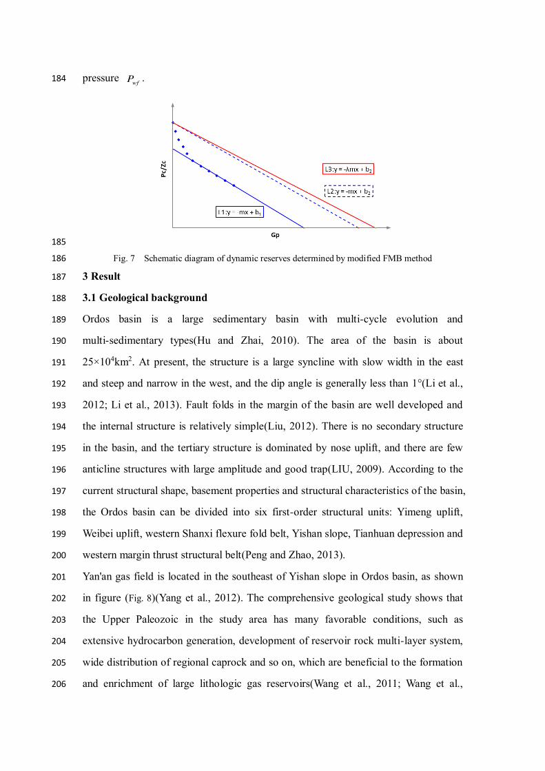
Fig. 7 Schematic diagram of dynamic reserves determined by modified FMB method 186

3 Result 187

3.1 Geological background 188

Ordos basin is a large sedimentary basin with multi-cycle evolution and 189

multi-sedimentary types(Hu and Zhai, 2010). The area of the basin is about 190

25×104km2. At present, the structure is a large syncline with slow width in the east 191

and steep and narrow in the west, and the dip angle is generally less than 1°(Li et al., 192

2012; Li et al., 2013). Fault folds in the margin of the basin are well developed and 193

the internal structure is relatively simple(Liu, 2012). There is no secondary structure 194

in the basin, and the tertiary structure is dominated by nose uplift, and there are few 195

anticline structures with large amplitude and good trap(LIU, 2009). According to the 196

current structural shape, basement properties and structural characteristics of the basin, 197

the Ordos basin can be divided into six first-order structural units: Yimeng uplift, 198

Weibei uplift, western Shanxi flexure fold belt, Yishan slope, Tianhuan depression and 199

western margin thrust structural belt(Peng and Zhao, 2013). 200

Yan'an gas field is located in the southeast of Yishan slope in Ordos basin, as shown 201

in figure (Fig. 8)(Yang et al., 2012). The comprehensive geological study shows that 202

the Upper Paleozoic in the study area has many favorable conditions, such as 203

extensive hydrocarbon generation, development of reservoir rock multi-layer system, 204

wide distribution of regional caprock and so on, which are beneficial to the formation 205

and enrichment of large lithologic gas reservoirs(Wang et al., 2011; Wang et al., 206

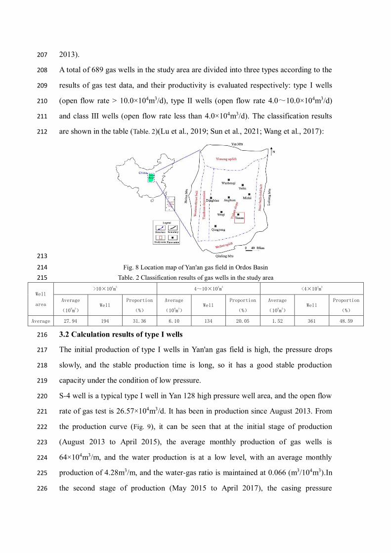
2013). 207

A total of 689 gas wells in the study area are divided into three types according to the 208

results of gas test data, and their productivity is evaluated respectively: type Ⅰ wells 209

(open flow rate > 10.0×104m3/d), type Ⅱ wells (open flow rate 4.0～10.0×104m3/d) 210

and class Ⅲ wells (open flow rate less than 4.0×104m3/d). The classification results 211

are shown in the table (Table. 2)(Lu et al., 2019; Sun et al., 2021; Wang et al., 2017): 212

213

Fig. 8 Location map of Yan'an gas field in Ordos Basin 214

Table. 2 Classification results of gas wells in the study area 215

Well

area

>10×104m3 4～10×10

4m3 <4×10

4m3

Average

（108m3）

Well Proportion

（%）

Average

（108m3）

Well Proportion

（%）

Average

（108m3）

Well Proportion

（%）

Average 27.94 194 31.36 6.10 134 20.05 1.52 361 48.59

3.2 Calculation results of type I wells 216

The initial production of type I wells in Yan'an gas field is high, the pressure drops 217

slowly, and the stable production time is long, so it has a good stable production 218

capacity under the condition of low pressure. 219

S-4 well is a typical type I well in Yan 128 high pressure well area, and the open flow 220

rate of gas test is 26.57×104m3/d. It has been in production since August 2013. From 221

the production curve (Fig. 9), it can be seen that at the initial stage of production 222

(August 2013 to April 2015), the average monthly production of gas wells is 223

64×104m3/m, and the water production is at a low level, with an average monthly 224

production of 4.28m3/m, and the water-gas ratio is maintained at 0.066 (m3/104m3).In 225

the second stage of production (May 2015 to April 2017), the casing pressure 226

decreases rapidly, the oil pressure decreases rapidly, the monthly water production is 227

higher, and the monthly gas production decreases rapidly. In the third stage of 228

production (May 2017 to April 2020), the monthly gas production and monthly water 229

production are kept at a low level, casing pressure is about 7MPa, and the oil pressure 230

is about 8MPa. Up to now, the cumulative gas production of S-4 well is 231

3633.775×104m3 and the cumulative water production is 356.67m3. 232

Fig. 9 S-4 well production curve

Fig. 10 S-4 calculation results of dynamic reserves

Using production data and wellhead casing pressure, draw Pc/Zc~Gp curve, as shown 233

in figure (Fig. 10). The linear fitting is carried out for the data points showing a 234

straight line trend, and the slope of the straight line is -0.0024. The slope of the 235

straight line passes through the Pi/Zi point as a straight line, and the intercept on the 236

Abscissa is 0.8737×108m8, which is the dynamic reserve of S-4 well determined by 237

the FMB method. 238

The calculation results show that -λ=-0.6387, -λm=-0.0015. Taking -λm as the slope 239

and making a straight line through the Pi/Zi point, the intercept on the Abscissa is 240

1.3980×108m8, which is the dynamic reserve of well S-4 determined by the modified 241

FMB method. 242

3.3 Calculation results of type Ⅱ wells 243

The test production of type II wells in the study area is between 4.0×104m3/d and 244

10.0×104m3/d, and the pressure drops rapidly, accounting for 20.048% of the number 245

of wells in the whole area. 246

S-5 well is a typical type Ⅱ well in Yan 128 high pressure well area (Fig. 11). 190 days 247

of trial production operation was carried out in S-5 well from November 19, 2009 to 248

May 27, 2010, and 70 days of pressure recovery test was carried out from May 27 to 249

August 7, 2010. The open flow rate of gas test in this well is 4.7045×104m3/d, and the 250

original formation pressure is 25.872 MPa. The production starts at 1.5×104m3/d. Due 251

to the large pressure fluctuation in the trial production process, the gas production is 252

difficult to be stable, and the working system is adjusted, the daily gas production is 253

gradually reduced to about 1×104m3/d, and the daily water production is 0.1～1.8 254

m3/d. After the gas production is reduced to 1×104m3/d, the oil pressure decreases 255

from 14.41MPa to 12.36MPa, a decrease of 2.05 MPa, and the oil pressure decreases 256

at a rate of 0.051MPa/d, which shows that the production is basically stable. Up to 257

April 2020, the cumulative gas production is 3471.62×104m3 and the cumulative 258

water production is 490.25m3. 259








the FMB method. 265




FMB method. 269

3.4 Calculation results of type Ⅲ wells 270

The initial production of type Ⅲ wells in the study area is low, about 35×104m3/m, 271

and the current production is 20×104m3/m. It has a certain stable production capacity 272

under the condition of low pressure. If the allocation of production is reduced, it can 273

be produced steadily for a long time. 274

S-6 well is a typical type Ⅲ well in this area, and the open flow rate of gas test is 275

8.944×104m3/d. It has been in production since June 2013. From the production curve 276

(Fig. 13), it can be seen that at the initial stage of production (June 2013 to December 277

2014), the average monthly production of gas wells is 50×104m3/m, the water 278

production is at a low level, the average monthly production is 3.02m3/m, and the 279

water-gas ratio is maintained at 0.060 (m3/104m3). In the second stage of production 280

(from January 2015 to June 2018), the casing pressure decreased rapidly and the 281

monthly gas production remained unchanged. In the third stage of production (July 282

2018 to April 2020), the monthly gas production decreases rapidly, the monthly water 283

production increases rapidly, the casing pressure is kept at about 8.5MPa, and the oil 284

pressure is maintained at about 7.8MPa. Up to now, the cumulative gas production of 285

S-6 is 2580.92×104m3, and the cumulative water production is 237.55m3. 286








the FMB method. 292




FMB method. 296

4 Discussion 297

Compared with the FMB method, the material balance method uses the average 298

formation pressure data measured after shut-in for a long time, so its calculation result 299

is more real and reliable(Fan et al., 2012; GAO et al., 2009). 300

4.1 Method verification 301

In order to verify the accuracy of the calculation results of the modified FMB method, 302

as shown in the table (Table. 3), using the measured formation pressure at different 303

stages of the production of the three wells, the scatter diagram between the cumulative 304

gas production and the measured Pzag Z is drawn (Fig. 15, Fig. 16, Fig. 17). 305

By linear fitting these discrete data points, the dynamic reserves of single well 306

calculated by three kinds of well material balance method can be obtained(Xu et al., 307

2014; Xu et al., 2016). ① The dynamic reserve of single well in S-4 is 308

1.3849×108m8 calculated by material balance method. By comparing the above 309

calculation results, the error of FMB method is 36.91%, and the error of modified 310

FMB method is 0.95% (Table. 4, Fig. 18).②The dynamic reserve of single well in S-5 311

is 1.1864×108m8 calculated by material balance method. By comparing the above 312


FMB method is 1.80 % (Table. 4, Fig. 18).③The dynamic reserve of single well in S-6 314

is 1.0086×108m8 calculated by material balance method. By comparing the above 315


FMB method is 1.00 % (Table. 4, Fig. 18). 317

Through the above calculation results (Fig. 18), compared with the material balance 318

method, the calculation result of the FMB method is generally small, with an average 319

error of 33.95%; the error of the modified FMB method is small, with an average of 320

1.25%(Li et al., 2018). Therefore, it can be concluded that when there is a lack of 321

measured pressure data, the calculation result of the modified FMB method is more 322

accurate than that of the FMB method. 323

Table. 3 Measured pressure in three wells 324

Time S4 S5 S6

Gp(104m3) P(MPa) P/Z Gp(104m3) P(MPa) P/Z Gp(104m3) P(MPa) P/Z

201312 268.355 18.800 20.567 135.008 18.923 20.727 216.712 18.713 20.515

201406 434.815 18.276 20.018 265.966 18.386 20.091 450.907 18.281 20.023

201412 787.525 17.918 19.589 431.721 18.147 19.893 546.945 17.644 19.321

201506 1211.685 17.617 19.152 720.386 17.578 19.273 767.195 17.980 19.659

201512 1522.465 16.668 18.186 990.256 17.360 18.988 971.055 16.738 18.231

201606 1836.965 16.488 17.915 1278.196 16.565 18.069 1200.765 16.678 18.048

325

Fig. 15 calculation of dynamic reserves by pressure drop method



Fig. 18 Calculation error of dynamic reserves

Table. 4 Calculation results of FMB method and modified FMB method 326

Well MBA(104m3) Mobile MBA(104m3) Error(%) Modified Mobile MBA(104m3) Error(%)

S4 13848.68 8737.50 36.91 13980.00 0.95

S5 11864.04 8065.38 32.02 11650.00 1.80

S6 10086.19 6764.52 32.93 9985.71 1.00

Average 11932.97 7855.80 33.95 11871.90 1.25

4.2 Application 327

Three dynamic reserve methods are used to calculate 31 typical gas wells in the study 328

area, and the results are shown in the table (Table. 5). The average reserves calculated 329

by the material balance method and the FMB method are 1.2731×108m8 and 330

0.6794×108m8, respectively. The minimum error is 28.499%, the maximum is 331

58.816%, and the average is 44.536%. The average error of the modified FMB 332

method is 1.3008×108m8, the minimum error is 1.290%, the maximum value is 333

3.063%, and the average is 2.114%. It is worth noting that the single wells with large 334

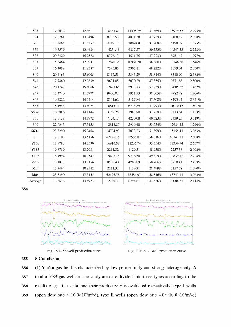
errors in the calculation results of the modified FMB method are S-56 and S-60-1. 335

Combined with the production data of two wells, S-56 well was put into production in 336

June 2013 (Fig. 19), and the shut-in state appeared intermittently from June 2013 to 337

December 2016, the pressure recovery state was in a short time, which reflected that 338

the formation pressure and casing pressure drop in the early stage of production were 339

relatively small, and the gas production per unit pressure drop was relatively 340

large(Mattar et al., 2006). Because there is no intermittent shut-in in the later stage of 341

production, the law of monthly gas production verifies this theory. Therefore, it can be 342

concluded that the early shut-in leads to the large dynamic reserves of a single well. 343

Similarly, the S-60-1 well was put into production in July 2015 (Fig. 20), and the 344

intermittent shut-in occurred in the later stage of production, and the production law 345

of the gas well could not fully reflect the real state of the gas well, resulting in a large 346

calculation error. 347

It can be seen that the great change in the production system of gas wells will affect 348

the accuracy of the calculation results of the modified FMB method, especially the 349

shut-in for a long time before calculating the pressure drop gas production at a certain 350

time. Therefore, time data points with relatively stable production should be selected 351

as far as possible to calculate the dynamic reserves of a single well. 352

Table. 5 Calculation results of three dynamic reserve methods 353

WELL

Initial wellhead

casing

pressure(MPa)

Pseudo steady

wellhead casing

pressure(MPa)

MBA Mobile MBA Modified Mobile MBA

Reserves

(104m3)

Reserves

(104m3) Error(%)

Reserves

(104m3) Error(%)

S1 15.8462 12.8592 7153.74 4282.75 40.133% 7342.40 2.637%

S12 17.1079 13.4597 14160.04 6336.27 55.252% 14370.62 1.487%

S14 18.7003 12.8507 10602.13 5843.84 44.881% 10833.20 2.179%

S15 17.3198 14.2056 12111.63 8659.90 28.499% 12334.85 1.843%

S16 18.0042 14.2344 12881.02 6668.23 48.232% 13183.31 2.347%

S18 20.9695 14.9531 9300.99 5114.52 45.011% 9482.64 1.953%

S19 19.1588 13.4765 15158.98 7982.84 47.339% 15426.74 1.766%

S2 16.6048 12.7247 4488.28 2515.88 43.946% 4560.57 1.611%

S20 20.9194 15.9530 23281.23 11621.87 50.081% 23693.58 1.771%

S23 17.2632 12.3611 18463.87 11508.79 37.669% 18979.53 2.793%

S24 17.8761 13.3496 8295.53 4831.38 41.759% 8488.67 2.328%

S3 15.3464 11.4357 4419.17 3009.09 31.908% 4498.07 1.785%

S36 16.7579 13.4424 14231.18 9857.57 30.733% 14547.33 2.222%

S37 20.8429 15.2572 8776.13 4631.75 47.223% 8951.42 1.997%

S38 15.3464 12.7981 17870.36 10961.70 38.660% 18146.58 1.546%

S39 16.4099 11.9387 7545.85 3907.11 48.222% 7699.04 2.030%

S40 20.4163 15.6005 8117.51 3343.29 58.814% 8310.90 2.382%

S41 17.7460 12.0839 9631.05 5070.29 47.355% 9871.88 2.500%

S42 20.1747 15.6066 12423.66 5933.73 52.239% 12605.25 1.462%

S47 15.4740 11.0778 9600.02 5951.53 38.005% 9782.98 1.906%

S48 19.7822 14.7414 8301.62 5187.84 37.508% 8495.94 2.341%

S53 18.1943 13.6024 10815.71 6273.89 41.993% 11010.45 1.801%

S53-1 16.5886 14.4144 3168.25 1987.80 37.259% 3213.64 1.433%

S56 17.5138 14.1972 7124.17 4230.08 40.623% 7339.25 3.019%

S60 22.6343 17.3155 12818.85 5956.40 53.534% 12984.22 1.290%

S60-1 23.8290 15.3464 14704.97 7073.23 51.899% 15155.41 3.063%

S8 17.9103 13.5156 62126.78 25586.07 58.816% 63747.11 2.608%

Y170 17.9788 14.2530 16910.98 11236.74 33.554% 17356.94 2.637%

Y185 19.8759 13.2931 2211.32 1129.31 48.930% 2257.58 2.092%

Y196 18.4994 10.9542 19406.76 9736.50 49.829% 19839.12 2.228%

Y202 18.1875 13.3156 8538.40 4208.89 50.706% 8750.41 2.483%

Min 15.3464 10.9542 2211.32 1129.31 28.499% 2257.58 1.290%

Max 23.8290 17.3155 62126.78 25586.07 58.816% 63747.11 3.063%

Average 18.3638 13.6973 12730.33 6794.81 44.536% 13008.37 2.114%

354


Fig. 20 S-60-1 well production curve

5 Conclusion 355

(1) Yan'an gas field is characterized by low permeability and strong heterogeneity. A 356

total of 689 gas wells in the study area are divided into three types according to the 357

results of gas test data, and their productivity is evaluated respectively: type Ⅰ wells 358

(open flow rate > 10.0×104m3/d), type Ⅱ wells (open flow rate 4.0～10.0×104m3/d) 359

and class Ⅲ wells (open flow rate less than 4.0×104m3/d). 360

(2) Through theoretical calculation and numerical simulation, it is found that the 361

viscosity of natural gas increases rapidly with the increase of pressure, the 362

compression coefficient of natural gas decreases at first (P<15MPa) and then 363

increases with the increase of pressure (P>15MPa), and increases with the increase of 364

temperature. Under the condition of low pressure, the compression coefficient and 365

volume coefficient of natural gas decrease rapidly with the increase of pressure and 366

increase with the increase of temperature. 367

(3) Considering the viscosity, compression coefficient and deviation coefficient of 368

natural gas, the FMB method is modified, and the calculation method and steps are 369

given at the same time. 370

(4) Verified by the production data of three types of typical gas wells, the results show 371

that compared with the calculation results of the material balance method, the average 372

error of the FMB method is 33.95%, and the average error of the modified FMB 373

method is 1.25%. 374

(5) The new method is used to calculate the dynamic reserves of 31 gas wells in the 375

study area. the results show that the great change of the production system of gas 376

wells will affect the accuracy of the modified FMB method, especially the shut-in for 377

a long time before the pressure drop gas production is calculated at a certain time, so 378

the points with relatively stable production should be selected as far as possible to 379

calculate the dynamic reserves of a single well. 380

Remarks 381

Z: Deviation coefficient of natural gas； 382

Vactual: The volume of a real gas, m3; 383

Videal: The volume of ideal gas, m3; 384

Cg: Natural gas compression coefficient； 385

Bg: Volume coefficient of natural gas； 386

VR: Underground volume of natural gas, m3； 387

Vsc: Volume of natural gas under surface conditions, m3； 388

cP : Wellhead casing pressure, MPa； 389

ciP : Original wellhead casing pressure, MPa； 390

wfP : Bottom hole flow pressure, MPa； 391

wfiP : Original bottom hole flow pressure, MPa。 392

pG : Cumulative gas production, 104m3； 393

P : Average formation pressure, MPa； 394

wfp : Bottom hole flow pressure, MPa； 395

Z : Deviation coefficient of natural gas under average formation pressure； 396

wfZ : Deviation coefficient of natural gas under bottom hole flow pressure； 397

gu : Viscosity of natural gas under average formation pressure, mPa·s； 398

gwfu : Viscosity of natural gas under bottom hole flow pressure, mPa·s； 399

gC : Compression coefficient of natural gas under average formation pressure, MPa-1； 400

gwfC : Compression coefficient of natural gas under bottom hole flow pressure, MPa-1。 401

pssP : Average formation pressure at the initial stage of pseudo steady state, MPa； 402

wf pssP : Bottom hole flow pressure at the initial stage of pseudo steady state, MPa； 403

iP : Original formation pressure, MPa； 404

gu : Viscosity of natural gas, mPa·s； 405

gC : Compression coefficient of natural gas, MPa-1； 406

: g g gwf gwfu c u c 。 407

Acknowledgement 408

This study was supported by the National Major Project 409

(2017ZX05008-004-004-001). The authors would like to thank the editors and 410

anonymous reviewers for their valuable suggestions for this paper. 411

Author contributions 412

Hongjun Cui, Lin Zhou and Qinghai Liu performed the experiments. Jie He, 413

Xiangdong Guo and Kaiyu Lei wrote the main manuscript. Yushuang Zhu and Linyu 414

Liu advised the students and corrected the manuscript. All authors reviewed the 415

manuscript. 416

Competing interests 417

The authors declare no competing interests. 418

Reference 419

Chen, G. and Che, X., 2011. Domain Material Balance Method for Low Permeability Gas-Oil Reservoir 420

by Depletion Drive Process. Xinjiang Petroleum Geology, 32(2): 157-159. 421

Cheng, S., Li, J., Li, X., Yang, F. and Wang, Y., 2005. Estimation of Gas Well Dynamic Reserves by 422

Integration of Material Balance Equation with Binomial Productivity Equation. Xinjiang 423

Petroleum Geology, 26(2): 181-182. 424

Fan, X., Liu, B., Bao, J., Kui, M. and Cao, J., 2012. Dynamic Analysis of Influencing Factors of Reserves in 425

the Sebei 1 Gas Field. Natural Gas Geoscience, 23(5): 939-943. 426

GAO, Q.-f., Dang, Y.-q., LI, J.-t., Yang, S.-b. and Shen, S.-f., 2009. Dynamic Reserves Calculation and 427

Evaluation of Sebei Gas Field in Qaidam Basin. Xinjiang Petroleum Geology, 30(4): 499-500. 428

Han, G. et al., 2019. Determination of pore compressibility and geological reserves using a new form 429

of the flowing material balance method. Journal of Petroleum Science and Engineering, 172: 430

1025-1033. 431

He, Z., Li, S., Zhang, F., Zhang, Q. and Li, B., 2019. Application of Dynamic Reserve Analysis in the 432

Recovery of Fault-Block Water Invasion Reservoir. Special Oil & Gas Reservoirs, 26(6): 98-102. 433

Hu, W. and Zhai, G., 2010. Practice and sustainable development of oil and nature gas exploration and 434

development in Ordos Basin. Engineering Science, 12(5): 64-72. 435

Huang, Q. et al., 2015. Study on theoretical basis of "flowing" material balance. Reservoir Evaluation 436

and Development, 5(5): 30-33,49. 437

Li, S. and Qiao, D., 2012. Current situation of tight sand gas in China. In: Q.J. Xu, H.H. Ge and J.X. Zhang 438

(Editors), Natural Resources and Sustainable Development, Pts 1-3. Advanced Materials 439

Research, pp. 85-+. 440

Li, X. et al., 2018. Correlation between per-well average dynamic reserves and initial absolute open 441

flow potential (AOFP) for large gas fields in China and its application. Petroleum Exploration 442

and Development, 45(6): 1088-1093. 443

Li, Y., Zhong, J., Li, X., Xu, J. and Chen, X., 2012. Characteristics of lower Jurassic tight sandstone gas 444

reservoirs in Baka area of Tuha Basin. Special Oil & Gas Reservoirs, 19(2): 29-32,136. 445

Li, Z., Jiang, Z., Pang, X., Li, F. and Zhang, B., 2013. Genetic Types of the Tight Sandstone Gas Reservoirs 446

in the Kuqa Depression,Tarim Basin,NW China. Earth Science, 38(1): 156-164. 447

Liu, R., 2012. Discussion on the Dynamic Reserve Calculation in Early Development Stage of Gas 448

Reservoir. Special Oil & Gas Reservoirs, 19(5): 69-72. 449

LIU, X.-h., 2009. A discussion on several key parameters of gas reservoir dynamic reserves calculation. 450

Natural Gas Industry, 29(9): 71-74. 451

Lu, K. et al., 2019. Dynamic reserves calculated by linear relationship in the early development of 452

water-drive gas reservoir. Lithologic Reservoirs, 31(1): 153-158. 453

Mattar, L., Anderson, D. and Stotts, G., 2006. Dynamic material balance - oil- or gas-in-place without 454

shut-ins. Journal of Canadian Petroleum Technology, 45(11): 7-10. 455

Nie, X., Chen, J. and Yuan, S., 2018. Experimental Study on Stress Sensitivity Considering Time Effect 456

for Tight Gas Reservoirs. Mechanika, 24(6): 784-789. 457

Peng, S. and Zhao, W., 2013. The adaptability study for developing tight gas reservoirs using horizontal 458

wells. In: L. Zheng et al. (Editors), Applied Materials and Technologies for Modern 459

Manufacturing, Pts 1-4. Applied Mechanics and Materials, pp. 614-617. 460

Shults, O., 2020. Method for calculating material balance of complex process flowcharts. Journal of 461

Mathematical Chemistry, 58(6): 1281-1290. 462

Sun, H. et al., 2021. A material balance based practical analysis method to improve the dynamic 463

reserve evaluation reliability of ultra-deep gas reservoirs with ultra-high pressure. Natural 464

Gas Industry B. 465

Wang, J. et al., 2011. Characteristic of Tight Sandstone Gas Reservoir in Tuha Basin and Its Exploration 466

Target. Xinjiang Petroleum Geology, 32(1): 14-17. 467

Wang, M., Fan, Z., Luo, W., Song, H. and Ding, J., 2017. Error Analysis of Dynamic Reserve Calculation 468

in Multi-Layer Loose Sandstone Gas Reservoir. Special Oil & Gas Reservoirs, 24(6): 100-106. 469

Wang, Y. et al., 2013. Comparison of Ordos and Foreign Similar Basins and Prediction for Mesozoic Oil 470

Reserves in Ordos Basin. Geoscience, 27(5): 1244-1250. 471

Wei, X. et al., 2017. New geological understanding of tight sandstone gas. Lithologic Reservoirs, 29(1): 472

11-20. 473

Xin, C., Wang, Y., Xu, Y., Shi, L. and Du, Y., 2018. Tight Gas Reservoir Dynamic Reserve Calculation with 474

Modified Flowing Material Balance. Special Oil & Gas Reservoirs, 25(2): 95-98. 475

Xu, M., Ran, Q., Li, N. and Shen, G., 2014. Effect of Sealed Boundary on Fluid Flow in Fractured Well in 476

Deformable Tight Gas Reservoir. Special Oil & Gas Reservoirs, 21(5): 92-94. 477

Xu, Y., Adefidipe, O. and Dehghanpour, H., 2016. A flowing material balance equation for two-phase 478

flowback analysis. Journal of Petroleum Science and Engineering, 142: 170-185. 479

Yang, H., Fu, J., Liu, X. and Meng, P., 2012. Accumulation conditions and exploration and development 480

of tight gas in the Upper Paleozoic of the Ordos Basin. Petroleum Exploration and 481

Development, 39(3): 295-303. 482

Yang, X., Lei, Y., Ma, D., Wang, L. and Wen, H., 2019. Application of new method of calculating dynamic 483

reserves in Bohai Oilfield. Fault Block Oil & Gas Field, 26(3): 329-332. 484

Yao, J. et al., 2015. Gas Control Factors and Evaluation Application of Tight Sandstone Gas Reservoirs. 485

Well Logging Technology, 39(4): 482-485,490. 486

Yin, W., Wu, Y. and Yu, J., 2019. Key Influencing Factor Analysis of the SEC Dynamic Reserve in Liaohe 487

Oilfield. Special Oil & Gas Reservoirs, 26(2): 86-90. 488

Yu, X., Liu, H., Cao, J. and Pang, J., 2012. The Research on Material Balance Considering In-Seam and 489

Intrabed Water. In: X. Zhou and Z.Z. Lei (Editors), Fluid Dynamic and Mechanical & Electrical 490

Control Engineering. Applied Mechanics and Materials, pp. 420-+. 491

Zhang, L., Zhang, L., Jiang, B. and Liu, H., 2013a. The method of dynamic reserves prediction for a 492

constant volume gas reservoir. In: G. Li and C. Chen (Editors), Applied Mechanics and 493

Materials I, Pts 1-3. Applied Mechanics and Materials, pp. 456-+. 494

Zhang, L., Zhang, L., Zhang, J., Lan, F. and Deng, P., 2013b. Calculation methods of the dynamic 495

reserves for gas wells in a low-permeability gas reservoir. In: X. Tang, W. Zhong, D. Zhuang, C. 496

Li and Y. Liu (Editors), Progress in Environmental Protection and Processing of Resource, Pts 497

1-4. Applied Mechanics and Materials, pp. 3243-+. 498

Zhong, H., Zhou, J., Li, Y., Pu, H. and Tan, Y., 2012. Dynamic reserve calculation of single well of low 499

permeability gas reservoir based on flowing material balance method. Lithologic Reservoirs, 500

24(3): 108-111. 501

502

Documents

Tight Gas Reservoir Dynamic Reserve Calculation with