Tighter Security Proofs for GPV-IBE in the

Quantum Random Oracle Model

Shuichi Katsumata*†, Shota Yamada†, and Takashi Yamakawa‡

*The University of Tokyoshuichi katsumata@it.k.u-tokyo.ac.jp

†National Institute of Advanced Industrial Science and Technology (AIST)yamada-shota@aist.go.jp

‡NTT Secure Platform Laboratoriesyamakawa.takashi@lab.ntt.co.jp

November 20, 2018

Abstract

In (STOC, 2008), Gentry, Peikert, and Vaikuntanathan proposed the first identity-basedencryption (GPV-IBE) scheme based on a post-quantum assumption, namely, the learningwith errors (LWE) assumption. Since their proof was only made in the random oracle model(ROM) instead of the quantum random oracle model (QROM), it remained unclear whetherthe scheme was truly post-quantum or not. In (CRYPTO, 2012), Zhandry developed newtechniques to be used in the QROM and proved security of GPV-IBE in the QROM, henceanswering in the affirmative that GPV-IBE is indeed post-quantum. However, since the generaltechnique developed by Zhandry incurred a large reduction loss, there was a wide gap betweenthe concrete efficiency and security level provided by GPV-IBE in the ROM and QROM.Furthermore, regardless of being in the ROM or QROM, GPV-IBE is not known to have atight reduction in the multi-challenge setting. Considering that in the real-world an adversarycan obtain many ciphertexts, it is desirable to have a security proof that does not degradewith the number of challenge ciphertext.

In this paper, we provide a much tighter proof for the GPV-IBE in the QROM in thesingle-challenge setting. In addition, we also show that a slight variant of the GPV-IBEhas an almost tight reduction in the multi-challenge setting both in the ROM and QROM,where the reduction loss is independent of the number of challenge ciphertext. Our proofdeparts from the traditional partitioning technique and resembles the approach used in thepublic key encryption scheme of Cramer and Shoup (CRYPTO, 1998). Our proof strategyallows the reduction algorithm to program the random oracle the same way for all identitiesand naturally fits the QROM setting where an adversary may query a superposition of allidentities in one random oracle query. Notably, our proofs are much simpler than the one byZhandry and conceptually much easier to follow for cryptographers not familiar with quantumcomputation. Although at a high level, the techniques used for the single and multi-challengesetting are similar, the technical details are quite different. For the multi-challenge setting,we rely on the Katz-Wang technique (CCS, 2003) to overcome some obstacles regarding theleftover hash lemma.

Keywords. Identity-based encryption, quantum random oracle models, LWE assumption,tight security reduction, multi-challenge security.

1

Contents

1 Introduction 31.1 Background . . . . . . . . . . . . . . . . . . . . . . . . . . . . . . . . . . . . . . . . 31.2 Our Contribution . . . . . . . . . . . . . . . . . . . . . . . . . . . . . . . . . . . . . 41.3 Technical Overview . . . . . . . . . . . . . . . . . . . . . . . . . . . . . . . . . . . . 41.4 Discussion. . . . . . . . . . . . . . . . . . . . . . . . . . . . . . . . . . . . . . . . . 81.5 Related Work . . . . . . . . . . . . . . . . . . . . . . . . . . . . . . . . . . . . . . . 9

2 Preliminaries 102.1 Quantum Computation . . . . . . . . . . . . . . . . . . . . . . . . . . . . . . . . . 102.2 Pseudorandom Function. . . . . . . . . . . . . . . . . . . . . . . . . . . . . . . . . . 112.3 Identity-Based Encryption . . . . . . . . . . . . . . . . . . . . . . . . . . . . . . . . 122.4 Background on Lattices . . . . . . . . . . . . . . . . . . . . . . . . . . . . . . . . . 13

3 Tightly Secure Single Challenge GPV-IBE 163.1 Construction . . . . . . . . . . . . . . . . . . . . . . . . . . . . . . . . . . . . . . . 163.2 Correctness and Parameter Selection . . . . . . . . . . . . . . . . . . . . . . . . . . 173.3 Security Proof in ROM . . . . . . . . . . . . . . . . . . . . . . . . . . . . . . . . . 183.4 Security Proof in QROM . . . . . . . . . . . . . . . . . . . . . . . . . . . . . . . . 21

4 (Almost) Tightly Secure Multi-Challenge IBE 244.1 Randomness Extraction . . . . . . . . . . . . . . . . . . . . . . . . . . . . . . . . . 244.2 Construction . . . . . . . . . . . . . . . . . . . . . . . . . . . . . . . . . . . . . . . 264.3 Correctness and Parameter Selection . . . . . . . . . . . . . . . . . . . . . . . . . . 274.4 Security Proof in ROM . . . . . . . . . . . . . . . . . . . . . . . . . . . . . . . . . 284.5 Security Proof in QROM . . . . . . . . . . . . . . . . . . . . . . . . . . . . . . . . 31

2

1 Introduction

1.1 Background

Shor [Sho94] in his breakthrough result showed that if a quantum computer is realized, then almostall cryptosystems used in the real world will be broken. Since then, a significant amount of studieshave been done in the area of post-quantum cryptography, whose motivation is constructingcryptosystems secure against quantum adversaries. Recently in 2016, the National Institute ofStandards and Technology (NIST) initiated the Post-Quantum Cryptography Standardization,and since then post-quantum cryptography has been gathering increasingly more attention.

Random Oracles in Quantum World. In general, security proofs of practical cryptographicschemes are given in the random oracle model (ROM) [BR93], which is an idealized model wherea hash function is modeled as a publicly accessible oracle that computes a random function.Boneh et al. [BDF+11] pointed out that the ROM as in the classical setting is not reasonablewhen considering security against quantum adversaries, since quantum adversaries may computehash functions over quantum superpositions of many inputs. Considering this fact, as a reasonablemodel against quantum adversaries, they proposed a new model called the quantum random oraclemodel (QROM), where a hash function is modeled as a quantumly accessible random oracle. Asdiscussed in [BDF+11], many commonly-used proof techniques in the ROM do not work in theQROM. Therefore even if we have a security proof in the ROM, we often require new techniquesto obtain similar results in the QROM.

Identity-based Encryption in QROM. Identity-Based Encryption (IBE) is a generalizationof a public key encryption scheme where the public key of a user can be any arbitrary stringsuch as an e-mail address. The first IBE scheme based on a post-quantum assumption is theone proposed by Gentry, Peikert and Vaikuntanathan (GPV-IBE) [GPV08], which is based onthe learning with errors (LWE) assumption [Reg05]. To this date, GPV-IBE is still arguably themost efficient IBE scheme that is based on a hardness assumption that resists quantum attacks.However, since their original security proof was made in the ROM instead of the QROM, it wasunclear if we could say the scheme is truly post-quantum. Zhandry [Zha12b] answered this inthe affirmative by proving that the GPV-IBE is indeed secure in the QROM under the LWEassumption, hence truly post-quantum, by developing new techniques in the QROM.

Tight Security of GPV-IBE. However, if we consider the tightness of the reduction, the securityproof of the GPV-IBE by Zhandry [Zha12b] does not provide satisfactory security. Specifically,GPV-IBE may be efficient in the ROM, but it is no longer efficient in the QROM. In general, acryptographic scheme is said to be tightly secure under some assumption if breaking the securityof the scheme is as hard as solving the assumption. More precisely, suppose that we proved that ifthere exists an adversary breaking the security of the scheme with advantage ε and running time T ,we can break the underlying assumption with advantage ε′ and running time T ′. We say that thescheme is tightly-secure if we have ε′/T ′ ≈ ε/T . By using this notation, Zhandry gave a reductionfrom the security of GPV-IBE to the LWE assumption with ε′ ≈ ε2/(QH + QID)4 and T ′ ≈T + (QH +QID)2 · poly(λ) where QH denotes the number of hash queries, QID denotes the numberof secret key queries, λ denotes the security parameter, and poly denotes some fixed polynomial.Though the reduction is theoretically interesting, the meaning of the resulting security bound ina realistic setting is unclear. For example, if we want to obtain 128-bit security for the resultingIBE, and say we had ε = 2−128, QH = 2100, QID = 220, then even if we ignore the blowup forthe running time, we would have to start from at least a 656-bit secure LWE assumption, whichincurs a significant blowup of the parameters. Indeed, Zhandry left it as an open problem to give

3

a tighter reduction for the GPV-IBE.

Multi-Challenge Tightness. The standard security notion of IBE considers the setting wherean adversary obtains only one challenge ciphertext. This is because security against adversariesobtaining many challenge ciphertexts can be reduced to the security in the above simplified setting.However, as pointed out by Hofheinz and Jager [HJ12], tightness is not preserved in the abovereduction since the security degrades by the number of ciphertexts. Therefore tightly secure IBEin the single-challenge setting does not imply tightly secure IBE in the multi-challenge setting.On the other hand, in the real world, it is natural to assume that an adversary obtains manyciphertexts, and thus tight security in the multi-challenge setting is desirable. However, there isno known security proof for the GPV-IBE or its variant that does not degrade with the numberof challenge ciphertexts even in the classical setting.

1.2 Our Contribution

We provide much tighter security proofs for the GPV-IBE in the QROM in the single-challengesetting. Furthermore, we provide a multi-challenge tight variant of GPV-IBE that is secure bothin the ROM and QROM. In the following, we describe the tightness of our security proofs byusing the same notation as in the previous section.

• In the single-challenge setting, we give a reduction from the security of GPV-IBE to theLWE assumption with ε′ ≈ ε and T ′ = T + (QH + QID)2 · poly(λ). If we additionallyassume quantumly secure pseudorandom functions (PRFs), then we further obtain a tighterreduction, which gives ε′ ≈ ε and T ′ = T + (QH + QID) · poly(λ). This is the first securityproof for GPV-IBE whose security bound does not degrade with QH or QID even in theclassical setting. We note that the same security bound can be achieved without assumingPRFs in the classical ROM.

• We give a slight variant of GPV-IBE scheme whose multi-challenge security is reduced tothe LWE assumption with ε′ = ε/poly(λ) and T ′ ≈ T + (QH + QID + Qch)2 · poly(λ) whereQch denotes the number of challenge queries. If we additionally assume quantumly securePRFs, then we further obtain a tighter reduction. Namely, ε′ is the same as the above, andT ′ = T + (QH +QID +Qch) ·poly(λ). This is the first variant of the GPV-IBE scheme whosesecurity bound does not degrade with Qch even in the classical setting. We note that thesame security bound can be achieved without assuming PRFs in the classical ROM.

Moreover, our security proofs are much simpler than the one by Zhandry [Zha12b]. In his work, heintroduced new techniques regarding indistinguishability of oracles against quantum adversaries.Though his techniques are general and also useful in other settings (e.g., [Zha12a]), it involvessome arguments on quantum computation, and they are hard to follow for cryptographers whoare not familiar with quantum computation. On the other hand, our proofs involve a minimalamount of discussions about quantum computation, and our proofs are done almost similar tothe counterparts in the classical ROM.

1.3 Technical Overview

GPV-IBE. First, we briefly describe the GPV-IBE [GPV08], which is the main target of thispaper. A master public key is a matrix A ∈ Zn×mq and a master secret key is its trapdoorTA ∈ Zm×m, which enables one to compute a short vector e ∈ Zmq such that Ae = u given anarbitrary vector u ∈ Znq . A private key skID for an identity ID ∈ ID is a short vector e ∈ Zmq

4

such that Ae = uID where uID = H(ID) for a hash function H : ID → Znq , which is modeled as

a random oracle. A ciphertext for a message M ∈ 0, 1 consists of c0 = u>IDs + x + Mbq/2e andc1 = A>s + x. Here s is a uniformly random vector over Znq and x,x are small “noise” termswhere each entries are sampled from some specific Gaussian distribution χ. Decryption can bedone by computing w = c0 − c>1 eID ∈ Zq and deciding if w is closer to 0 or to bq/2e modulo q.

Security Proof in Classical ROM. The above IBE relies its security on the LWE assumption,

which informally states the following: given a uniformly random matrix [A|u] ← Zn×(m+1)q and

some vector b ∈ Zm+1q , there is no PPT algorithm that can decide with non-negligible proba-

bility whether b is of the form [A|u]>s + x′ for some s ← Znq and x′ ← χm+1, or a uniformlyrandom vector over Zm+1

q , i.e., b ← Zm+1q . Below, we briefly recall the original security proof

in the classical ROM given by Gentry et al. [GPV08] and see how the random oracle is used bythe reduction algorithm. The proof relies on a key lemma which states that we can set H(ID)and e in the “reverse order” from the real scheme. That is, we can first sample e from somedistribution and program H(ID) := Ae so that their distributions are close to uniformly randomas in the real scheme. In the security proof, a reduction algorithm guesses i ∈ [Q] such that theadversary’s i-th hash query is the challenge identity ID∗ where Q denotes the number of hashqueries made by the adversary. Then for all but the i-th hash query, the reduction algorithmprograms H(ID) in the above manner, and for the i-th query, it programs the output of H(ID∗)to be the vector u contained in the LWE instance that is given as the challenge. Specifically,the reduction algorithm sets the challenge user’s identity vector uID∗ as the random vector ucontained in the LWE instance. If the guess is correct, then it can embed the LWE instance intothe challenge ciphertexts c∗0 and c∗1; in case it is a valid LWE instance, then (c∗0, c

∗1) is properly set

to (u>ID∗s + x+ Mbq/2e,A>s + x) as in the real scheme. Therefore, the challenge ciphertext canbe switched to random due to the LWE assumption. After this switch, M is perfectly hidden andthus the security of GPV-IBE is reduced to the LWE assumption. Since the reduction algorithmprograms the random oracle in the same way except for the challenge identity, this type of proofmethodology is often times referred to as the “all-but-one programming”.

Security Proof in QROM in [Zha12b]. Unfortunately, the above proof cannot be simplyextended to a proof in the QROM. The reason is that in the QROM, even a single hash querycan be a superposition of all the identities. In such a case, to proceed with the above all-but-one programming approach, the reduction algorithm would have to guess a single identity outof all the possible identities which he hopes that would be used as the challenge identity ID∗ bythe adversary. Obviously, the probability of the reduction algorithm being right is negligible,since the number of possible identities is exponentially large. This is in sharp contrast with theROM setting, where the reduction algorithm was allowed to guess the single identity out of thepolynomially many (classical) random oracle queries made by the adversary. Therefore, the all-but-one programming as in the classical case cannot be used in the quantum case. To overcome thisbarrier, Zhandry [Zha12b] introduced a useful lemma regarding what he calls the semi-constantdistribution. The semi-constant distribution with parameter 0 < p < 1 is a distribution overfunctions from X to Y such that a function chosen according to the distribution gives the samefixed value for random p-fraction of all inputs, and behaves as a random function for the rest ofthe inputs. He proved that a function according to the semi-constant distribution with parameterp and a random function cannot be distinguished by an adversary that makes Q oracle querieswith advantage greater than 8

3Q4p2. In the security proof, the reduction algorithm partitions the

set of identities into controlled and uncontrolled sets. The uncontrolled set consists of randomly

5

chosen p-fraction of all identities, and the controlled set is the complement of it. The reductionalgorithm embeds an LWE instance into the uncontrolled set, and programs the hash values forthe controlled set so that the decryption keys for identities in the controlled set can be extractedefficiently. Then the reduction algorithm works as long as the challenge identity falls inside theuncontrolled set and all identities for secret key queries fall inside the controlled set (otherwiseit aborts). By appropriately setting p, we can argue that the probability that the reductionalgorithm does not abort is non-negligible, and thus the security proof is completed. Though thistechnique is very general and useful, a huge reduction loss is inherent as long as we take the abovestrategy because the reduction algorithm has to abort with high probability. It may be useful topoint out for readers who are familiar with IBE schemes in the standard model that the abovetechnique is conceptually very similar to the partitioning technique which is often used in thecontext of adaptively secure IBE scheme in the standard model [Wat05, ABB10, CHKP10]. Thereason why we cannot make the proof tight is exactly the same as that for the counterparts inthe standard model.

Our Tight Security Proof in QROM. As discussed above, we cannot obtain a tight reductionas long as we use a partitioning-like technique. Therefore we take a completely different approach,which is rather similar to that used in the public key encryption scheme of Cramer and Shoup[CS98], which has also been applied to the pairing-based IBE construction of Gentry [Gen06].The idea is that we simulate in a way so that we can create exactly one valid secret key for everyidentity. Note that this is opposed to the partitioning technique (and the all-but-one programmingtechnique) where the simulator cannot create a secret key for an identity in the uncontrolled set.To create the challenge ciphertext, we use the one secret key we know for that challenge identity.If the adversary can not tell which secret key the ciphertext was created from and if there arepotentially many candidates for the secret key, we can take advantage of the entropy of the secretkey to statistically hide the message.

In more detail, the main observation is that the secret key e, i.e. a short vector e such thatAe = u, retains plenty of entropy even after fixing the public values A and u. Therefore, byprogramming the hash value u of an identity, we can easily create a situation where the simulatorknows exactly one secret key out of the many possible candidates. Furthermore, the simulatorknowing a secret key eID∗ such that AeID∗ = uID∗ , can simulate the challenge ciphertext bycreating c∗0 = e>ID∗c

∗1 + Mbq/2e and c∗1 = A>s + x. Here, the key observation is that we no

longer require the LWE instance (uID∗ ,u>ID∗s + x) to simulate the challenge ciphertext. Though

the distribution of c∗0 simulated as above is slightly different from that of the real ciphertext dueto the difference in the noise distributions, we ignore it in this overview. In the real proof, weovercome this problem by using the noise rerandomization technique by Katsumata and Yamada[KY16]. Then we use the LWE assumption to switch c∗1 to random. Finally, we argue thate>ID∗c

∗1 is almost uniform if the min-entropy of eID∗ is high and c∗1 is uniformly random due to the

leftover hash lemma. Therefore, all information of the message M is hidden and thus the proof iscompleted.

Finally, we observe that the above proof naturally fits in the QROM setting. The crucialdifference from the partitioning technique is that in our security proof we program the randomoracle in the same way for all identities. Therefore even if an adversary queries a superpositionof all identities, the simulator can simply quantumly perform the programming procedure for thesuperposition. Thus the proof in the classical ROM can be almost automatically converted intothe one in the QROM.

Tight Security in Multi-Challenge Setting. Unfortunately, the above idea does not extendnaturally to the tightly-secure multi-challenge setting. One can always prove security in the multi-

6

challenge setting starting from a scheme that is single-challenge secure via a hybrid argument,however, as mentioned by Hofheinz and Jager [HJ12], this type of reduction does not preservetightness. A careful reader may think that the above programming technique can be extendedto the multi-challenge setting, hence bypassing the hybrid argument. We briefly explain whythis is not the case. Informally, in the above proof, the reduction algorithm embeds its givenLWE instance (A,A>s+x) into the challenge ciphertext by creating (c∗0 = e>ID∗c

∗1 +Mbq/2e, c∗1 =

A>s+x), where eID∗ is the secret key of the challenge user uID∗ . Therefore, since the c∗1 componentof every ciphertext is an LWE instance for the same public matrix A, to simulate multiple challengeciphertexts in the above manner, the reduction algorithm must be able to prepare a special type ofLWE instance (A, A>s(k) +x(k)k∈[N ]), where N = poly(λ) is the number of challenge ciphertextqueried by the adversary. It can be easily seen that this construction is tightly-secure in the multi-challenge setting with the same efficiency as the single-challenge setting, if we assume that thisspecial type of LWE problem is provided to the reduction algorithm as the challenge. However,unfortunately, we still end up losing a factor of N in the reduction when reducing the standardLWE problem to this special LWE problem. In particular, we only shifted the burden of havingto go through the N hybrid arguments to the assumption rather than to the scheme. As one mayhave noticed, there is a way to bypass the problem of going through the N hybrid argumentsby using conventional techniques (See [Reg05, Reg10]) of constructing an unlimited number offresh LWE instances given a fixed number of LWE instances. However, this techniques requiresthe noise of the newly created LWE instances to grow proportionally to the number of createdinstances. In particular, to create the above special LWE instance from a standard LWE instance,we require the size of the noise x(k) to grow polynomially with N , where recall that N can bean arbitrary polynomial. Hence, although we can show a tightly secure reduction in the multi-challenge setting, for the concrete parameters of the scheme to be independent of N , we needto assume the LWE assumption with super-polynomial modulus size to cope with the super-polynomial noise blow up. This is far more inefficient than in the single-challenge setting wherewe only had to require an LWE assumption with polynomial modulus size.

To overcome this problem, we use the “lossy mode” of the LWE problem. It is well knownthat the secret vector s is uniquely defined given an LWE instance (A,A>s + x) for large enoughsamples. A series of works, e.g., [GKPV10, BKPW12, AKPW13, LSSS17] have observed that ifwe instead sample A from a special distribution that is computationally indistinguishable fromthe uniform distribution, then (A,A>s + x) leaks almost no information of the secret s, hencethe term “lossy mode”. This idea can be leveraged to prove (almost) tight security of the abovesingle-challenge construction, where the reduction loss is independent of the number of challengeciphertext. A first attempt of using this idea is as follows: During the security proof of the GPV-IBE, we first change the public matrix A to a lossy matrix A and generate the secret keys andprogram the random oracle in the same way as before. To create the challenge ciphertexts, thereduction algorithm honestly samples s(k), x(k), x(k) and sets (c∗0 = u>ID∗s

(k)+x(k)+M(k)bq/2e, c∗1 =

A>s(k)+x(k)). Now, it may seem that owing to the lossy mode of LWE, we can rely on the entropyof the secret vector s(k) to argue that c∗0 is distributed uniformly random via the leftover hashlemma. The main difference between the previous single-challenge setting is that we can rely onthe entropy of the secret vector s(k) rather than on the entropy of the secret key eID∗ . Since eachchallenge ciphertext is injected with fresh entropy and we can argue statistically that a singlechallenge ciphertext is not leaking any information on the message, the reduction loss will beindependent of the number of challenge ciphertext query N .

Although the above argument may seem correct at first glance, it incurs a subtle but a fatalflaw, thus bringing us to our proposed construction. The problem of the above argument is how

7

we use the leftover hash lemma. To use the lemma correctly, the vector uID∗ viewed as a hashfunction is required to be universal. This is true in case uID∗ is set as AeID∗ , where A ← Zn×mq

and eID∗ is sampled from some appropriate distribution. However, this is not true anymore oncewe change A to a lossy matrix A, since A now lives in an exponentially small subset of Zn×mq ,

and uID∗ is no longer universal. Specifically, we can no longer rely on the entropy of s(k) tostatistically hide the message. To overcome this problem, our final idea is to use the Katz-Wang[KW03] technique. Specifically, we slightly alter the encryption algorithm of GPV-IBE to outputthe following instead:

c0 = u>ID||0s + x0 + Mbq/2e, c1 = u>ID||1s + x1 + Mbq/2e, and c2 = A>s + x,

where uID||b = H(ID||b) for b ∈ 0, 1. During the security proof, the reduction algorithm setsuID||0 and uID||1 so that one of them is uniformly random over Znq and the other is constructedas AeID. Then, for the ciphertext cb corresponding to the uniformly random vector uID||b, wecan correctly use the leftover hash lemma to argue that cb statistically hides the message M. Bygoing through one more hybrid argument, we can change both c0, c1 into random values that areindependent of the message M. Note that instead of naively using the Katz-Wang technique, byreusing the c2 component, the above GPV-IBE variant only requires one additional element in Zqcompared to the original GPV-IBE. Furthermore, in the actual construction, we do not requirethe noise terms x0, x1 in c0, c1 since we no longer rely on the LWE assumption to change c0, c1

into random values. Our construction and security reduction does not depend on the number ofchallenge ciphertext query N and in particular, can be proven under the LWE assumption withpolynomial modulus size. In addition, due to the same reason as the single-challenge setting, ourclassical ROM proof can be naturally converted to a QROM proof.

1.4 Discussion.

Similar Techniques in Other Works. The idea to simulate GPV-IBE in a way so that wecan create exactly one valid secret key for every secret key query is not new. We are aware of fewworks that are based on this idea. Gentry, Peikert and Vaikuntanathan [GPV08] mentioned thatby using this technique, they can prove the security of the GPV-IBE in the standard model basedon a non-standard interactive variant of the LWE (I-LWE) assumption which requires a hashfunction to define. Here since the hash function is given to the adversary, a quantum adversarymay query quantum states to the hash functions on its own. Therefore, in addition with thefact that the I-LWE assumption is made in the standard model, the statement made by [GPV08]would hold in the QROM as well. However, they only gave a sketch of the proof, and did not givea formal proof. Alwen et al. [ADN+10] use the idea to construct an identity-based hash proofsystem (IB-HPS) based on the mechanism of GPV-IBE. We note that they assume the modulusq to be super-polynomial. Outside the context of identity-based primitives, Applebaum et al.[ACPS09] and Bourse et al. [BDPMW16] provide an analysis of rerandomizing LWE sampleswhich can be seen as a refinement of the idea mentioned in [GPV08]. [ACPS09] constructs aKDM-secure cryptosystem based on the LWE problem and [BDPMW16] shows a simple methodfor constructing circuit private fully homomorphic encryption schemes (FHE) based on the lattice-based FHE scheme of Gentry et al. [GSW13]. Both of their analysis only requires the modulusq to be polynomial. In summary, though similar ideas have been used, all of the previous worksare irrelevant to tight security or the security in the QROM.

On Parameter-Tightness of Our Schemes. In the above overview, we focused on the tightnessof the security proof. Here, we provide some discussions on how the parameters compare to the

8

original GPV-IBE scheme [GPV08]. For the single challenge setting, our parameters are only asmall factor worse than the GPV-IBE scheme. This is because the only difference is using thenoise rerandomization technique of [KY16], which only slightly degrades the noise-level.1 For themulti-challenge setting, the situation is more different. In this case, the parameters are muchworse than the original (single-challenge secure) GPV-IBE scheme. This is because we have to gothrough the lossy-mode of LWE which requires for larger parameters. The concrete parametersare provided in Sec. 4.3.

Relation to CCA-Secure PKE. By applying the Canetti-Halevi-Katz transformation [CHK04]to our single-challenge-secure IBE scheme, we obtain a public key encryption (PKE) scheme secureagainst chosen ciphertext attacks (CCA) that is tightly secure in the single-challenge setting underthe LWE assumption in the QROM. We note that Saito et al. [SXY18] already proposed sucha PKE scheme in the single-challenge setting that is more efficient than the scheme obtained bythe above transformation.

On Running Time of Reductions. In the above overview, we ignore the running time ofreductions. Though it seems that the above described reductions run in nearly the same time asthe adversaries, due to a subtle problem of simulating random oracles against quantum adversaries,there is a significant blowup by a square factor of the number of queries the adversaries make.In the classical ROM, when we simulate a random oracle in security proofs, we usually samplea random function in a lazy manner. That is, whenever an adversary queries a point that hasnot been queried before, a reduction algorithm samples a fresh randomness and assigns it as ahash value for that point. However, this cannot be done in the QROM because an adversary mayquery a superposition of all the inputs in a single query. Therefore a reduction algorithm has tosomehow commit to the hash values of all inputs at the beginning of the simulation.

Zhandry [Zha12b] proved that an adversary that makes Q queries cannot distinguish a randomfunction and a 2Q-wise independent hash function via quantum oracle accesses. Therefore we canuse a 2Q-wise independent hash to simulate a random oracle. However, if we take this method,the simulator has to evaluate a 2Q-wise independent hash function for each hash query, and thisis the reason why the running time blowups by Ω(Q2).

One possible way to avoid this huge blowup is to simulate a random oracle by a PRF secureagainst quantum accessible adversaries. Since the time needed to evaluate a PRF is some fixedpolynomial in the security parameter, the blowup for the running time can be made Q · poly(λ)which is significantly better than Ω(Q2). However, in order to use this method, we have toadditionally assume the existence of quantumly secure PRFs. Such PRFs can be constructed basedon any quantumly-secure one-way function [Zha12a], and thus they exist if the LWE assumptionholds against quantum adversaries. However, the reduction for such PRFs are non-tight and thuswe cannot rely on them in the context of tight security. Our suggestion is to use a real hashfunction to implement PRFs and to assume that it is a quantumly secure PRF. We believe thisto be a natural assumption if we are willing to idealize a hash function as a random oracle. (Seealso the discussion in Sec. 2.2.)

1.5 Related Work

Schemes in QROM. Boneh et al. [BDF+11] introduced the QROM, and gave security proofsfor the GPV-signature [GPV08] and a hybrid variant of the Bellare-Rogaway encryption [BR93]

1 Our parameter selection in the main body may seem much worse compared to GPV-IBE, but this is onlybecause we choose the parameters conservatively. Specifically, we can set the parameters to be only slightly worsethan GPV-IBE by setting them less conservatively as in [GPV08]. Please, see end of Sec. 3.2 for more details.

9

in the QROM. We note that their security proof for the GPV-signature is tight. Zhandry [Zha12b]proved that GPV-IBE and full-domain hash signatures are secure in the QROM. Targhi and Unruh[TU16] proposed variants of Fujisaki-Okamoto transformation and OAEP that are CCA securein the QROM. Jiang et al. [JZC+18] gave tighter security proofs for some variants of Fujisaki-Okamoto transformation. Some researchers studied the security of the Fiat-Shamir transform inthe QROM [ARU14, Unr15, Unr17]. Unruh [Unr14b] proposed a revocable quantum timed-releaseencryption scheme in the QROM. Unruh [Unr14a] proposed a position verification scheme in theQROM. Recently, some researchers studied tight securities in the QROM. Alkim et al. [ABB+17]proved that the signature scheme known as TESLA [BG14] is tightly secure under the LWEassumption. Saito et al. [SXY18] proposed a tightly CCA secure variant of the Bellare-Rogawayencryption. Kiltz et al. [KLS18] gave a tight reduction for the Fiat-Shamir transform in theQROM.Tightly Secure IBEs. The first tightly secure IBE scheme from lattices in the single chal-lenge setting and in the standard model was proposed by Boyen and Li [BL16]. Recently, theyextended their results to the multi-challenge setting [BL18]. While both constructions are the-oretically interesting and elegant, they are very inefficient and requires LWE assumption withsuper-polynomial approximation factors. As for the construction from bilinear maps, the firsttightly secure IBE from standard assumptions in the single challenge setting and in the randomoracle model was proposed by Katz and Wang [KW03]. Coron [Cor09] gave a tight reduction fora variant of the original Boneh-Franklin IBE [BF01]. Later, the first realization in the standardmodel was proposed by Chen and Wee [CW13]. In the subsequent works, it is further extendedto the multi-challenge setting [HKS15, AHY15, GDCC16]. They are efficient but are not secureagainst quantum computers.

2 Preliminaries

Notations. For n ∈ N, denote [n] as the set 1, · · · , n. For a finite set S, we let U(S) denote theuniform distribution over S. For a distribution D and integer k > 0, define (D)k as the distribution∏i∈[k]D. For a distribution or random variable X we write x ← X to denote the operation of

sampling a random x according to X. For a set S, we write s← S as a shorthand for s← U(S).Let X and Y be two random variables over some finite set SX , SY , respectively. The statisticaldistance ∆(X,Y ) between X and Y is defined as ∆(X,Y ) = 1

2Σs∈SX∪SY |Pr[X = s]− Pr[Y = s]|.The min-entropy of a random variable X is defined as H∞(X) = − log(maxx Pr[X = x]), wherethe base of the logarithm is taken to be 2 throughout the paper. For a bit b ∈ 0, 1, b denotes 1−b.For sets X and Y, Func(X ,Y) denotes the set of all functions from X to Y. For a vector v ∈ Rn,denote ‖v‖ as the standard Euclidean norm. For a matrix R ∈ Rn×n, denote ‖R‖ as the lengthof the longest column and ‖R‖GS as the longest column of the Gram-Schmidt orthogonalizationof R.

2.1 Quantum Computation

We briefly give some backgrounds on quantum computation. We refer to [NC00] for more details.A state |ψ〉 of n qubits is expressed as

∑x∈0,1n αx |x〉 ∈ C2n where αxx∈0,1n is a set of

complex numbers such that∑

x∈0,1n |αx|2 = 1 and |x〉x∈0,1n is an orthonormal basis on C2n

(which is called a computational basis). If we measure |ψ〉 in the computational basis, then theoutcome is a classical bit string x ∈ 0, 1n with probability |αx|2, and the state becomes |x〉.An evolution of quantum state can be described by a unitary matrix U , which transforms |x〉 to

10

U |x〉. A quantum algorithm is composed of quantum evolutions described by unitary matricesand measurements. We also consider a quantum oracle algorithm, which can quantumly accessto certain oracles. The running time Time(A) of a quantum algorithm A is defined to be thenumber of universal gates (e.g., Hadamard, phase, CNOT, and π/8 gates) and measurementsrequired for running A. (An oracle query is counted as a unit time if A is an oracle algorithm.)Any efficient classical computation can be realized by a quantum computation efficiently. Thatis, for any function f that is classically computable, there exists a unitary matrix Uf such thatUf |x, y〉 = |x, f(x)⊕ y〉, and the number of universal gates to express Uf is linear in the size ofa classical circuit that computes f .

Quantum random oracle model. Boneh et al. [BDF+11] introduced the quantum randomoracle model (QROM), which is an extension of the usual random oracle model to the quantumsetting. Roughly speaking, the QROM is an idealized model where a hash function is idealizedto be a quantumly accessible oracle that simulates a random function. More precisely, in securityproofs in the QROM, a random function H : X → Y is uniformly chosen at the beginning ofthe experiment, and every entity involved in the system is allowed to access to an oracle that isgiven

∑x,y αx,y |x, y〉 and returns

∑x,y αx,y |x,H(x)⊕ y〉. We denote a quantum algorithm A that

accesses to the oracle defined as above by A|H〉. In the QROM, one query to the random oracle iscounted as one unit time. As in the classical case, we can implement two random oracles H0 andH1 from one random oracle H by defining H0(x) := H(0||x) and H1(x) := H(1||x). More generally,we can implement n random oracles from one random oracle by using the blog nc-bit prefix of aninput as indices of random oracles.

As shown by Zhandry [Zha12b], a quantum random oracle can be simulated by a family of2Q-wise independent hash functions against an adversary that quantumly accesses the oracle atmost Q times. As a result, he obtained the following lemma.

Lemma 1. ([Zha12b, Thereom 6.1].) Any quantum algorithm A making quantum queries torandom oracles can be efficiently simulated by a quantum algorithm B, which has the same outputdistribution, but makes no queries. Especially, if A makes at most Q queries to a random oracleH : 0, 1a → 0, 1b, then Time(B) ≈ Time(A) + Q · T 2Q-wise

a,b where T 2Q-wisea,b denotes the time to

evaluate a 2Q-wise independent hash function from 0, 1a to 0, 1b.

The following lemma was shown by Boneh et al. [BDF+11]. Roughly speaking, this lemmastates that if an oracle outputs independent and almost uniform value for all inputs, then it isindistinguishable from a random oracle even with quantum oracle accesses.

Lemma 2. ([BDF+11, Lem. 3].) Let A be a quantum algorithm that makes at most Q oraclequeries, and X and Y be arrbitrary sets. Let H be a distribution over Func(X ,Y) such that whenwe take H← H, for each x ∈ X , H(x) is identically and independently distributed according to adistribution D whose statistical distance is within ε from uniform. Then for any input z. we have

∆(A|RF〉(z),A|H〉(z)) ≤ 4Q2√ε

where RF← Func(X ,Y) and H← H.

2.2 Pseudorandom Function.

We review the definition of quantum-accessible pseudorandom functions (PRFs) [BDF+11].

11

Definition 1 (Quantum-accessible PRF). We say that a function F : K×X → Y is a quantum-accessible pseudorandom function if for all quantum polynomial time adversaries A, its advantagedefined below is negligible:

AdvPRFA,F (λ) :=∣∣∣Pr

[A|RF〉

(1λ)

= 1]− Pr

[A|F (K,·)〉(1λ) = 1

]∣∣∣where RF← Func(X ,Y) and K ← K.

Zhandry [Zha12a] proved that some known constructions of classical PRFs including the tree-based construction [GGM86] and lattice-based construction [BPR12] are also quantum-accessiblePRFs. However, these reductions are non-tight, and thus we cannot rely on these results whenaiming for tight security. Fortunately, we can use the following lemma which states that we canuse a quantum random oracle as a PRF similarly to the classical case.

Lemma 3. ([SXY18, Lem. 2.2]) Let ` be an integer. Let H : 0, 1`×X → Y and H′ : X → Y betwo independent random functions. If an unbounded time quantum adversary A makes a queryto H at most QH times, then we have∣∣∣Pr[A|H〉,|H(K,·)〉(1λ) = 1 | K ← 0, 1`]− Pr[A|H〉,|H′〉(1λ) = 1]

∣∣∣ ≤ QH · 2−`+1

2 .

2.3 Identity-Based Encryption

Syntax. We use the standard syntax of IBE [BF01]. Let ID be the ID space of the scheme. If acollision resistant hash function CRH : 0, 1∗ → ID is available, one can use an arbitrary stringas an identity. An IBE scheme is defined by the following four algorithms.

Setup(1λ)→ (mpk,msk): The setup algorithm takes as input a security parameter 1λ and outputsa master public key mpk and a master secret key msk.

KeyGen(mpk,msk, ID)→ skID: The key generation algorithm takes as input the master public keympk, the master secret key msk, and an identity ID ∈ ID. It outputs a private key skID. Weassume that ID is implicitly included in skID.

Encrypt(mpk, ID,M)→ C: The encryption algorithm takes as input a master public key mpk, anidentity ID ∈ ID, and a message M. It outputs a ciphertext C.

Decrypt(mpk, skID, C)→ M or ⊥: The decryption algorithm takes as input the master public keympk, a private key skID, and a ciphertext C. It outputs the message M or ⊥, which meansthat the ciphertext is not in a valid form.

Correctness. We require correctness of decryption: that is, for all λ, all ID ∈ ID, and all M inthe specified message space,

Pr[Decrypt(mpk, skID,Encrypt(mpk, ID,M)) = M] = 1− negl(λ)

holds, where the probability is taken over the randomness used in (mpk,msk) ← Setup(1λ),skID ← KeyGen(mpk,msk, ID), and Encrypt(mpk, ID,M).

Security. We now define the security for an IBE scheme Π. This security notion is defined by thefollowing game between a challenger and an adversary A. Let CTSam(·) be a sampling algorithmthat takes as input a master public key of the scheme and outputs an element in the ciphertextspace.

- Setup. At the outset of the game, the challenger runs Setup(1λ) → (mpk,msk) and gives mpkto A. The challenger also picks a random coin coin ← 0, 1 and keeps it secretly. After given

12

mpk, A can adaptively make the following two types of queries to the challenger. These queriescan be made in any order and arbitrarily many times.

Secret Key Queries. If A submits ID ∈ ID to the challenger, the challenger returns skID ←KeyGen(mpk,msk, ID).

Challenge Queries. If A submits a message M∗ and an identity ID∗ ∈ ID to the challenger,the challenger proceeds as follows. If coin = 0, it runs Encrypt(mpk, ID∗,M∗) → C∗ and givesthe challenge ciphertext C∗ to A. If coin = 1, it chooses the challenge ciphertext C∗ from thedistribution CTSam(mpk) as C∗ ← CTSam(mpk) at random and gives it to A.

We prohibit A from making a challenge query for an identity ID∗ such that it has alreadymade a secret key query for the same ID = ID∗ and vice versa.

- Guess. Finally, A outputs a guess coin for coin. The advantage of A is defined as

AdvIBEA,Π(λ) =

∣∣∣∣Pr[coin = coin]− 1

2

∣∣∣∣ .We say that Π is adaptively-anonymous secure, if there exists efficiently sampleable distributionCTSam(mpk) and the advantage of any PPT A is negligible in the above game. The term anony-mous captures the fact that the ciphertext does not reveal the identity for which it was sent to.(Observe that CTSam(mpk) depends on neither of ID∗ nor M∗.)

Single Challenge Security. We can also consider a variant of the above security definitionwhere we restrict the adversary to make the challenge query only once during the game. Wecall this security notion “single challenge adaptive anonymity”, and call the notion without therestriction “multi challenge security”. By a simple hybrid argument, we can show that thesedefinitions are in fact equivalent in the sense that one implies another. However, the proof thatthe former implies the latter incurs a huge security reduction loss that is linear in the numberof challenge queries. Since the focus of this paper is on tight security reductions, we typicallydifferentiate these two notions.

Remark 1. We say that an IBE scheme is stateful if the key generation algorithm has to recordall previously issued secret keys, and always outputs the same secret key for the same identity.By the technique by Goldreich [Gol86], a stateful scheme can be converted to a stateless one (inwhich the key generation algorithm need not remember previous executions) by using PRFs. SincePRFs exist in the QROM without assuming any computational assumption as shown in Lem. 3,if we make the key size of PRFs sufficiently large, this conversion hardly affects the tightness.Therefore in this paper, we concentrate on constructing tightly secure stateful IBE schemes forsimplicity.

2.4 Background on Lattices

A (full-rank-integer) m-dimensional lattice Λ in Zm is a set of the form ∑

i∈[m] xibi|xi ∈ Z,where B = b1, · · · ,bm are m linearly independent vectors in Zm. We call B the basis of thelattice Λ. For any positive integers n,m and q ≥ 2, a matrix A ∈ Zn×mq and a vector u ∈ Znq , we

define Λ⊥(A) = z ∈ Zm|Az = 0 mod q, and Λ⊥u (A) = z ∈ Zm|Az = u mod q.Gaussian Measures. For an m-dimensional lattice Λ, the discrete Gaussian distribution over Λwith center c and parameter σ is defined asDΛ,σ,c(x) = ρσ,c(x)/ρσ,c(Λ) for all x ∈ Λ, where ρσ,c(x)is a Gaussian function defined as exp(−π‖x−c‖2/σ2) and ρσ,c(Λ) =

∑x∈Λ ρσ,c(x). Further for an

m-dimensional shifted lattice Λ + t, we define the Gaussian distribution DΛ+t,σ with parameter

13

σ as the process of adding the vector t to a sample from DΛ,σ,−t. Finally, we call D a B-boundeddistribution, if all the elements in the support of D have absolute value smaller than B.

Discrete Gaussian Lemmas. The following lemmas are used to manipulate and obtain mean-ingful bounds on discrete Gaussian vectors.

Lemma 4 (Adopted from [GPV08], Lem. 5.2). Let n,m, q be positive integers such that m ≥2n log q and q a prime. Let σ be any positive real such that σ ≥

√n+ logm. Then for all but

2−Ω(n) fraction of A ∈ Zn×mq , we have that the distribution of u = Ae mod q for e ← DZm,σ is

2−Ω(n)-close to uniform distribution over Znq . Furthermore, for a fixed u ∈ Znq , the conditionaldistribution of e← DZm,σ, given Ae = u mod q is DΛ⊥u (A),σ.

The following lemma is obtained by combining Lem. 4.4 in [MR07] and Lem. 5.3 in [GPV08].

Lemma 5 ([MR07], [GPV08]). Let σ > 16√

log 2m/π and u be any vector in Znq . Then, for allbut q−n fraction of A ∈ Zn×mq , we have that

Prx←D

Λ⊥u ,σ(A)

[‖x‖ > σ√m] < 2−(m−1).

The following lemma can be obtained by a straightforward combination of Lem. 2.6, Lem. 2.10,and Lem. 5.3 in [GPV08] (See also [PR06, Pei07]).

Lemma 6 ([PR06, Pei07, GPV08]). Let σ > 16√

log 2m/π and u be any vector in Znq . Then, forall but q−n fraction of A ∈ Zn×mq , we have

H∞(DΛ⊥u (A),σ) ≥ m− 1.

The following is a useful lemma used during the security proof. It allows the simulator tocreate new LWE samples from a given set of LWE samples (i.e., the LWE challenge provided tothe simulator) for which it does not know the associating secret vector.2 We would like to notethat the following lemma is built on top of many previous results [Reg05, Pei10, BLP+13] and isformatted in a specific way to be useful in the security proof for LWE-based cryptosystems.

Lemma 7 (Noise Rerandomization, [KY16], Lem. 1). Let q, `,m be positive integers and r apositive real satisfying r > Ω(

√n). Let b ∈ Zmq be arbitrary and z chosen from DZm,r. Then there

exists a PPT algorithm ReRand such that for any V ∈ Zm×` and positive real σ > s1(V), theoutput of ReRand(V,b + z, r, σ) is distributed as b′ = V>b + z′ ∈ Z`q where the distribution of z′

is within 2−Ω(n) statistical distance of DZ`,2rσ.

Sampling Algorithms. The following lemma states useful algorithms for sampling short vec-tors from lattices. In particular, the second preimage sampler is the exact gaussian sampler of[BLP+13], Lem. 2.3.

Lemma 8. ([GPV08, MP12, BLP+13]) Let n,m, q > 0 be integers with m > 3ndlog qe.

− TrapGen(1n, 1m, q)→ (A,TA): a PPT algorithm that outputs a matrix A ∈ Zn×mq and a full-

rank matrix TA ∈ Zm×m, where TA is a basis for Λ⊥(A), the distribution of A is 2−Ω(n)-closeto uniform and ‖TA‖GS = O(

√n log q).

2 Compared to [KY16] our choice of parameter is more conservative since we consider 2−Ω(n) statistical distancerather than 2−ω(logn).

14

− SamplePre(A,TA,u, σ) : a PPT algorithm that, given a matrix A ∈ Zn×mq , a basis TA ∈ Zm×m

for Λ⊥(A), a vector u ∈ Znq and a Gaussian parameter σ > ‖TA‖GS ·√

log(2m+ 4)/π, outputs

a vector e ∈ Zm sampled from a distribution 2−Ω(n)-close to DΛ⊥u (A),σ.

− SampleZ(σ) : a PPT algorithm that, given a Gaussian parameter σ > 16(√

log 2m/π), outputsa vector e ∈ Zm sampled from a distribution 2−Ω(n)-close to DZm,σ.

Hardness Assumptions. We define the Learning with Errors (LWE) problem introduced byRegev [Reg05].

Definition 2 (Learning with Errors). For integers n = n(λ),m = m(n), a prime q = q(n) > 2, anerror distribution χ = χ(n) over Z, and a quantum polynomial time algorithm A, the advantagefor the learning with errors problem LWEn,m,q,χ of A is defined as follows:

AdvLWEn,m,q,χA =

∣∣∣Pr[A(A,A>s + z

)= 1]− Pr

[A(A,w + z

)= 1]∣∣∣

where A ← Zn×mq , s ← Znq , w ← Zmq , z ← χm. We say that the LWE assumption holds if

AdvLWEn,m,q,χA is negligible for all quantum polynomial time algorithm A.

The (decisional) LWEn,m,q,DZ,αq for αq > 2√n has been shown by Regev [Reg05] via a quantum

reduction to be as hard as approximating the worst-case SIVP and GapSVP problems to withinO(n/α) factors in the `2-norm in the worst case. In the subsequent works, (partial) dequantu-mization of the reduction were achieved [Pei09, BLP+13].

We also define the LWE assumption against adversaries that can access to a quantum randomoracle as is done by Boneh et al. [BDF+11].

Definition 3 (Learning with Errors relative to Quantum Random Oracle). Let n, m, q and χbe the same as in Def. 2, and a, b be some positive integers. For a quantum polynomial timealgorithm A, the advantage for the learning with errors problem LWEn,m,q,χ of A relative to aquantum random oracle is defined as follows:

AdvLWEn,m,q,χA,QROa,b

(λ) =∣∣∣Pr

[A|H〉

(A,A>s + z

)= 1]− Pr

[A|H〉

(A,w + z

)= 1]∣∣∣

where A← Zn×mq , s← Znq , w ← Zmq , z← χm, H← Func(0, 1a, 0, 1b). We say that the LWE

assumption relative to an (a, b)-quantum random oracle holds if AdvLWEn,m,q,χA,QROa,b

(λ) is negligible for

all quantum polynomial time algorithm A.

It is easy to see that the LWE assumption relative to a quantum random oracle can be reducedto the LWE assumption with a certain loss of the time for the reduction by Lem. 1. Alternatively,if we assume the existence of a quantumly-accessible PRF, then the reduction loss can be madesmaller. Namely, we have the following lemmas.

Lemma 9. For any n, m, q, χ, a, b, and a quantum polynomial time algorithm A making atmost Q oracle queries, there exists a quantum polynomial time algorithm B such that

AdvLWEn,m,q,χA,QROa,b

(λ) = AdvLWEn,m,q,χB (λ)

and Time(B) ≈ Time(A) + Q · T 2Q-wisea,b where T 2Q-wise

a,b denotes the time to evaluate a 2Q-wise

independent hash function from 0, 1a to 0, 1b.

15

Lemma 10. Let F : K × 0, 1a → 0, 1b be a quantumly-accessible PRF. For any n, m, q, χ,a, b and a quantum polynomial time algorithm A making at most Q oracle queries, there existsquantum polynomial time algorithms B and C such that

AdvLWEn,m,q,χA,QROa,b

(λ) ≤ AdvLWEn,m,q,χB (λ) + AdvPRFC,F (λ)

and Time(B) ≈ Time(A) +Q · TF and Time(C) ≈ Time(A) where TF denotes the time to evaluateF .

In this paper, we give reductions from the security of IBE schemes to the LWE assumptionrelative to a quantrum random oracle. Given such reductions, we can also reduce them to theLWE assumption or to the LWE assumption plus the security of quantumly-accessible PRFs byLem. 9 or 10, respectively. The latter is tighter than the former at the cost of assuming theexistence of quantumly-accessible PRFs.

Remark 2. A keen reader may wonder why we have to require the extra assumption on the exis-tence of PRFs when we are working in the QROM, since as we mentioned earlier in Sec. 2.2, itseems that we can use a QRO as a PRF. The point here is that during the security reduction, thesimulator (which is given the classical LWE instance) must simulate the QRO query to the adver-sary against the LWE problem relative to a quantum random oracle query, hence, the simulatoris not in possession of the QRO. Note that the reason why we are able to use the QRO as a PRFas mentioned in Rem. 1 is because the simulator is aiming to reduce the LWE problem relative toa quantum random oracle query to the IBE scheme. Specifically, in this case the simulator canuse the QRO provided by its challenge to simulate a PRF.

3 Tightly Secure Single Challenge GPV-IBE

In this section, we show that we can give a tight security proof for the original GPV-IBE [GPV08]in the single-challenge setting if we set the parameters appropriately. Such proofs can be given inboth the classical ROM and QROM settings.

3.1 Construction

Let the identity space ID of the scheme be ID = 0, 1`ID , where `ID(λ) denotes the identity-length. Let also H : 0, 1`ID → Znq be a hash function treated as a random oracle during securityanalysis. The IBE scheme GPV is given as follows. For simplicity, we describe the scheme as astateful one. As remarked in Rem. 1, we can make the scheme stateless without any additionalassumption in the QROM.

Setup(1λ): On input 1λ, it first chooses a prime q, positive integers n,m, and Gaussian parametersα′, σ, where all these values are implicitly a function of the security parameter λ. Theprecise parameter selection is specified in the following section. It then runs (A,TA) ←TrapGen(1n, 1m, q) to generate a matrix A ∈ Zn×mq with a trapdoor TA ∈ Zm×m such that‖TA‖GS ≤ O(n log q). Then it outputs

mpk = A and msk = TA

KeyGen(mpk,msk, ID): If skID is already generated, then this algorithm returns the same skID.Otherwise it computes uID = H(ID) and samples eID ∈ Zm such that

AeID = uID mod q

16

using eID ← SamplePre(A,TA,uID, σ). It returns skID = eID as the secret key.

Enc(mpk, ID,M): To encrypt a message M ∈ 0, 1, it first samples s ← Znq , x ← DZm,α′q andx← DZ,α′q. Then it sets uID = H(ID) and computes

c0 = u>IDs + x+ Mbq/2e, c1 = A>s + x.

Finally, it outputs the ciphertext C = (c0, c1) ∈ Zq × Zmq .

Dec(mpk, skID, C): To decrypt a ciphertext C = (c0, c1) with a secret key skID, it computesw = c0 − c>1 eID ∈ Zq and outputs 0 if w is closer to 0 than to bq/2e modulo q. Otherwise itoutputs 1.

3.2 Correctness and Parameter Selection

The following shows correctness of the above IBE scheme.

Lemma 11 (Correctness). Suppose the parameters q, σ, and α′ are such that

σ > ‖TA‖GS ·√

log(2m+ 4)/π, α′ < 1/8σm.

Let eID ← KeyGen(A,TA, ID), C ← Enc(A, ID′,M ∈ 0, 1) and M′ ← Dec(A, eID, C). If ID = ID′,then with overwhelming probability we have M′ = M.

Proof. When the Dec algorithm operates as specified, we have

w = c0 − e>IDc1 = Mbq/2e+ x+ e>IDx︸ ︷︷ ︸error term

.

By Lem. 8 and the condition posed on the choice of σ, we have that the distribution of eIDis 2−Ω(n) close to DΛ⊥u (A),σ. Therefore, by Lem. 5, we have |x| ≤ α′q

√m, ‖x‖ ≤ α′q

√m, and

‖eID‖ ≤ σ ·√m except for 2−Ω(n) probability. Then, the error term is bounded by

|x+ e>IDx| ≤ |x|+ ‖eID‖ · ‖x‖ ≤ 2α′qσm.

Hence, for the error term to have absolute value less than q/4, it suffices to choose q and α′ as inthe statement of the lemma.

Parameter Selection. For the system to satisfy correctness and make the security proof work,we need the following restrictions. Note that we will prove the security of the scheme under theLWE assumption whose noise rate is α, which is lower than α′ that is used in the encryptionalgorithm.

- The error term is less than q/4 (i.e., α′ < 1/8mσ by Lem. 11)

- TrapGen operates properly (i.e., m > 3n log q by Lem. 8)

- Samplable from DΛ⊥u (A),σ (i.e., σ > ‖TA‖GS ·√

log(2m+ 4)/π = O(√n logm log q) by Lem. 8),

- σ is sufficiently large so that we can apply Lem. 4 and 6 (i.e., σ >√n+ logm, 16

√log 2m/π),

- We can apply Lem. 7 (i.e., α′/2α >√n(σ2m+ 1)),

- LWEn,m,q,DZ,αq is hard (i.e., αq > 2√n).

17

To satisfy these requirements, for example, we can set the parameters m, q, σ, α, α′ as follows:

m = n1+κ, q = 10n3.5+4κ, σ = n0.5+κ,

α′q = n2+2κ, αq = 2√n,

where κ > 0 is a constant that can be set arbitrarily small. To withstand attacks running intime 2λ, we may set n = Ω(λ). In the above, we round up m to the nearest integer and q tothe nearest largest prime. We remark that though the above parameter is worse compared to theoriginal GPV-IBE scheme, this is due to our conservative choice of making the statistical errorterms appearing in the reduction cost 2−Ω(n) rather than the standard negligible notion 2−ω(log λ).The latter choice of parameters will lead to better parameters, which may be as efficient as theoriginal GPV-IBE.

3.3 Security Proof in ROM

The following theorem addresses the security of GPV in the classical ROM setting. Our analysisdeparts from the original one [GPV08] and as a consequence results in a much tighter reduction.

Theorem 1. The IBE scheme GPV is adaptively-anonymous single-challenge secure in the ran-dom oracle model assuming the hardness of LWEn,m,q,DZ,αq . Namely, for any classical PPT ad-versary A making at most QH random oracle queries to H and QID secret key queries, there existsa classical PPT algorithm B such that

AdvIBEA,GPV(λ) ≤ AdvLWEn,m,q,DZ,αqB (λ) + (QH +QID) · 2−Ω(n)

andTime(B) = Time(A) + (QH +QID) · poly(λ).

Proof of Theorem 1. Let CTSam(mpk) be an algorithm that outputs a random element fromZq × Zmq and A be a classical PPT adversary that attacks the adaptively-anonymous securityof the IBE scheme. Without loss of generality, we make some simplifying assumptions on A.First, we assume that whenever A queries a secret key or asks for a challenge ciphertext, thecorresponding ID has already been queried to the random oracle H. Second, we assume that Amakes the same query for the same random oracle at most once. Third, we assume that A doesnot repeat secret key queries for the same identity more than once. We show the security of thescheme via the following games. In each game, we define Xi as the event that the adversary Awins in Gamei.

Game0 : This is the real security game. At the beginning of the game, (A,TA)← TrapGen(1n, 1m, q)is run and the adversary A is given A. The challenger then samples coin ← 0, 1 and keeps itsecret. During the game, A may make random oracle queries, secret key queries, and the challengequery. These queries are handled as follows:

• When A makes a random oracle query to H on ID, the challenger chooses a random vectoruID ← Znq and locally stores the tuple (ID,uID,⊥), and returns uID to A.

• When the adversaryA queries a secret key for ID, the challenger computes eID = SamplePre(A,TA,uID, σ)and returns eID to A.

• When the adversary makes the challenge query for ID∗ and a message M∗, the challengerreturns (c0, c1)← Encrypt(mpk, ID,M) if coin = 0 and (c0, c1)← CTSam(mpk) if coin = 1.

18

At the end of the game, A outputs a guess coin for coin. Finally, the challenger outputs coin. Bydefinition, we have

∣∣Pr[X0]− 12

∣∣ =∣∣Pr[coin− coin]− 1

2

∣∣ = AdvIBEA,GPV(λ).

Game1 : In this game, we change the way the random oracle queries to H are answered. WhenA queries the random oracle H on ID, the challenger generates a pair (uID, eID) by first samplingeID ← DZm,σ and setting uID = AeID. Then it locally stores the tuple (ID,uID,⊥), and returns uID

to A. Here, we remark that when A makes a secret key query for ID, the challenger returns e′ID ←SamplePre(A,TA,uID, σ), which is independent from eID that was generated in the simulation ofthe random oracle H on input ID. Note that in this game, we only change the distribution of uID

for each identity. Due to Lem. 4, the distribution of uID in Game2 is 2−Ω(n)-close to that of Game1

except for 2−Ω(n) fraction of A since we choose σ >√n+ logm. Therefore, the statistical distance

between the view of A in Game1 and Game2 is 2−Ω(n) +QH · 2−Ω(n) < QH · 2−Ω(n). Therefore, wehave

∣∣Pr[X1]− Pr[X2]∣∣ = QH · 2−Ω(n).

Game2 : In this game, we change the way secret key queries are answered. By the end of thisgame, the challenger will no longer require the trapdoor TA to generate the secret keys. When Aqueries the random oracle on ID, the challenger generates a pair (uID, eID) as in the previous game.Then it locally stores the tuple (ID,uID, eID) and returns uID to A. When A queries a secret keyfor ID, the challenger retrieves the unique tuple (ID,uID, eID) from local storage and returns eID.

For any fixed uID ∈ Znq , let e(1)ID,uID

and e(2)ID,uID

be random variables that are distributed accordingto the distributions of skID conditioning on H(ID) = uID in Game1 and Game2, respectively.

Due to Lem. 8, we have ∆(e(1)ID,uID

, DΛ⊥u (A),σ) ≤ 2−Ω(n). On the other hand, due to Lem. 4, we

have ∆(e(2)ID,uID

, DΛ⊥u (A),σ) ≤ 2−Ω(n). Since A obtains at most QID user secret keys skID, we have∣∣Pr[X1]− Pr[X2]∣∣ = QID · 2−Ω(n).

Game3 : In this game, we change the way the matrix A is generated. Concretely, the challengerchooses A← Zn×mq without generating the associated trapdoor TA. By Lem. 8, this makes only

2−Ω(n)-statistical difference. Since the challenger can answer all the secret key queries withoutthe trapdoor due to the change we made in the previous game, the view of A is altered onlynegligibly. Therefore, we have

∣∣Pr[X2]− Pr[X3]∣∣ = 2−Ω(n).

Game4 : In this game, we change the way the challenge ciphertext is created when coin = 0. Recallin the previous games when coin = 0, the challenger created a valid challenge ciphertext as inthe real scheme. In this game, to create the challenge ciphertext for identity ID∗ and message bitM∗, the challenger first retrieves the unique tuple (ID∗,uID∗ , eID∗) from local storage. Then thechallenger picks s← Znq , x← DZm,αq and computes v = A>s + x ∈ Zmq . It then runs

ReRand([eID∗ |Im],v, αq,α′

2α)→ c′ ∈ Zm+1

q

from Lem. 7, where Im is the identity matrix with size m. Let c′0 ∈ Zq denote the first entry ofc′ and c1 ∈ Zmq denote the remaining entries of c′. Finally, the challenger outputs the challengeciphertext as

C∗ = (c0 = c′0 + M∗bq/2e, c1). (1)

We now proceed to bound |Pr[X3]−Pr[X4]|. We apply the noise rerandomization lemma (Lem. 7)with V = [eID∗ |Im], b = A>s and z = x to see that the distribution of c′ is negligibly close tothe following:

c′ = V>b + x′ =(A · [eID∗ |Im]

)>s + x′ = [uID∗ |A]>s + x′

19

where the distribution of x′ is 2−Ω(n)-close to DZm+1,α′q. Here, the last equality follows fromAeID∗ = uID∗ and we can appropriately apply the noise rerandomization lemma since we have thefollowing for our parameter selection:

α′/2α >√n(σ2m+ 1) ≥

√n(‖eID∗‖2 + 1) ≥

√n · s1([eID∗ |Im]),

where the second inequality holds with 1− 2−Ω(n) probability. It can be seen that the challengeciphertext is distributed statistically close to that in Game3. Therefore, we may conclude that∣∣Pr[X3]− Pr[X4]

∣∣ = 2−Ω(n).

Game5 : In this game, we further change the way the challenge ciphertext is created when coin = 0.If coin = 0, to create the challenge ciphertext the challenger first picks b ← Zmq , x ← DZm,αqand computes v = b + x ∈ Zmq . It then sets V = [eID∗ |Im] and runs the ReRand algorithm as inGame3. Finally, it sets the challenge ciphertext as in Eq. (1). We claim that

∣∣Pr[X4] − Pr[X5]∣∣

is negligible assuming the hardness of the LWEn,m,q,DZ,αq problem. To show this, we use A toconstruct an LWE adversary B as follows:

B is given a problem instance of LWE as (A,v = b + x) ∈ Zn×mq × Zmq where x ← DZm,αq.

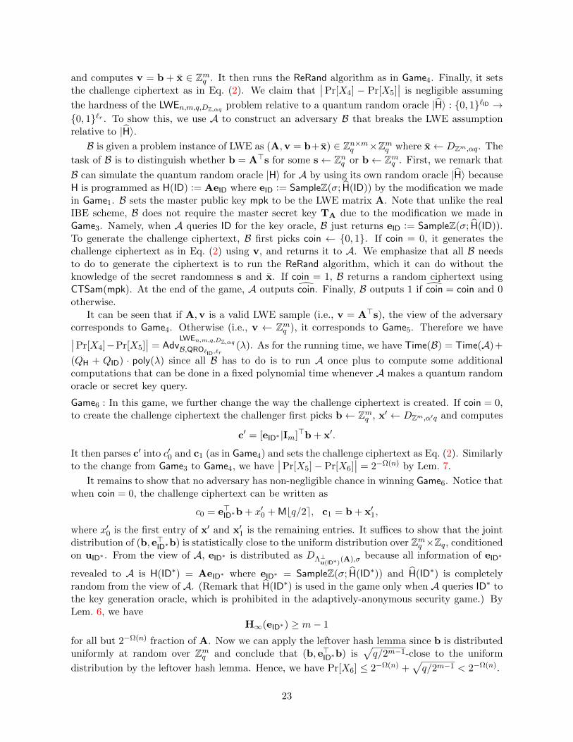
The task of B is to distinguish whether b = A>s for some s← Znq or b← Zmq . B sets the masterpublic key mpk to be the LWE matrix A. Note that unlike the real IBE scheme, B does notrequire the master secret key TA due to the modification we made in Game3. To generate thechallenge ciphertext, B first picks coin← 0, 1. If coin = 0, it generates the challenge ciphertextas in Eq. (1) using v, and returns it to A. We emphasize that all B needs to do to generate theciphertext is to run the ReRand algorithm, which it can do without the knowledge of the secretrandomness s and x. If coin = 1, B returns a random ciphertext using CTSam(mpk). At the end

of the game, A outputs coin. Finally, B outputs 1 if coin = coin and 0 otherwise. It can be seenthat if A,v is a valid LWE sample (i.e., v = A>s), the view of the adversary corresponds toGame4. Otherwise (i.e., v← Zmq ), it corresponds to Game5. We therefore conclude that assumingthe hardness of LWEn,m,q,DZ,αq problem we have

∣∣Pr[X4]− Pr[X5]∣∣ = negl.

Game6 : In this game, we change the way the challenge ciphertext is created once more. If coin = 0,to create the challenge ciphertext the challenger first picks b← Zmq , x′ ← DZm,α′q and computes

c′ = [eID∗ |Im]>b + x′.

It then parses c′ into c′0 and c1 (as in Game4) and sets the challenge ciphertext as Eq. (1). Similarlyto the change from Game3 to Game4, we have

∣∣Pr[X5]− Pr[X6]∣∣ = 2−Ω(n) by Lem. 7.

It remains to show that no adversary has negligible chance in winning Game6. Notice thatwhen coin = 0, the challenge ciphertext can be written as

c0 = e>ID∗b + x′0 + Mbq/2e, c1 = b + x′1,

where x′0 is the first entry of x′ and x′1 is the remaining entries. It suffices to show that the jointdistribution of (b, e>ID∗b) is negligibly close to the uniform distribution over Zmq ×Zq, conditionedon uID∗ . From the view of A, eID∗ is distributed as DΛ⊥uID∗

(A),σ. By Lem. 6, we have

H∞(eID∗) ≥ m− 1

for all but 2−Ω(n) fraction of A. Now we can apply the leftover hash lemma since b is distributeduniformly at random over Zmq and conclude that (b, e>ID∗b) is

√q/2m−1-close to the uniform

distribution. Hence, we have Pr[X6] ≤ 2−Ω(n) +√q/2m−1 < 2−Ω(n).

Therefore, combining everything together, the theorem is proven.

20

3.4 Security Proof in QROM

As we explained in the introduction, our analysis in the ROM can be easily be extended to theQROM setting. We can prove the following theorem that addresses the security of the GPV-IBEscheme in the QROM setting. The analysis here is different from that by Zhandry [Zha12b], whogave the first security proof for the GPV-IBE scheme in the QROM setting and our analysis hereis much tighter.

Theorem 2. The IBE scheme GPV is adaptively-anonymous single-challenge secure assumingthe hardness of LWEn,m,q,DZ,αq in the quantum random oracle model. Namely, for any quantumadversary A making at most QH queries to |H〉 and QID secret key queries, there exists a quantumalgorithm B making QH +QID quantum random oracle queries such that

AdvIBEA,GPV(λ) ≤ AdvLWEn,m,q,DZ,αqB,QRO`ID,`r

(λ) + (Q2H +QID) · 2−Ω(n)

andTime(B) = Time(A) + (QH +QID) · poly(λ)

where `r denotes the length of the randomness for SampleZ.

Proof of Theorem 2. Let CTSam(mpk) be an algorithm that outputs a random element fromZq × Zmq and A be a quantum adversary that attacks the adaptively-anonymous security of theIBE scheme. Without loss of generality, we can assume that A makes secret key queries on thesame identity at most once. We show the security of the scheme via the following games. In eachgame, we define Xi as the event that the adversary A wins in Gamei.

Game0 : This is the real security game for the adaptively-anonymous security. At the beginningof the game, the challenger chooses a random function H : 0, 1`ID → Znq . Then it generates(A,TA) ← TrapGen(1n, 1m, q) and gives A to A. Then it samples coin ← 0, 1 and keeps itsecret. During the game, A may make (quantum) random oracle queries, secret key queries, anda challenge query. These queries are handled as follows:

• When A makes a random oracle query on a quantum state∑

ID,y αID,y |ID〉 |y〉, the challengerreturns

∑ID,y αID,y |ID〉 |H(ID)⊕ y〉.

• WhenAmakes a secret key query on ID, the challenger samples eID = SamplePre(A,TA,uID, σ)and returns eID to A.

• When Amakes a challenge query for ID∗ and a message M∗, the challenger returns (c0, c1)←Encrypt(mpk, ID,M) if coin = 0 and (c0, c1)← CTSam(mpk) if coin = 1.

At the end of the game, A outputs a guess coin for coin. Finally, the challenger outputs coin. Bydefinition, we have

∣∣Pr[X0]− 12

∣∣ =∣∣Pr[coin− coin]− 1

2

∣∣ = AdvIBEA,GPV(λ).

Game1 : In this game, we change the way the random oracle H is simulated. Namely, the challengerfirst chooses another random function H← Func(0, 1`ID , 0, 1`r). Then we define H(ID) := AeIDwhere eID := SampleZ(σ; H(ID)), and use this H throughout the game. For any fixed ID, the dis-tribution of H(ID) is identical and its statistical distance from the uniform distribution is 2−Ω(n)

for all but 2−Ω(n) fraction of A due to Lem. 4 since we choose σ >√n+ logm . Note that in this

game, we only change the distribution of uID for each identity, and the way we create secret keys are

21

unchanged. Then due to Lem. 2, we have∣∣Pr[X0]−Pr[X1]

∣∣ = 2−Ω(n)+4Q2H

√2−Ω(n) = Q2

H ·2−Ω(n).

Game2 : In this game, we change the way secret key queries are answered. By the end of thisgame, the challenger will no longer require the trapdoor TA to generate the secret keys. WhenA queries a secret key for ID, the challenger returns eID := SampleZ(σ; H(ID)). For any fixed

uID ∈ Znq , let e(1)ID,uID

and e(2)ID,uID

be random variables that are distributed according to thedistributions of eID conditioning on H(ID) = uID in Game1 and Game2, respectively. Due to

Lem. 8, we have ∆(e(1)ID,uID

, DΛ⊥uID(A),σ) ≤ 2−Ω(n). On the other hand, due to Lem. 4, we have

∆(e(2)ID,uID

, DΛ⊥uID(A),σ) ≤ 2−Ω(n). Since A obtains at most QID user secret keys eID, we have∣∣Pr[X1]− Pr[X2]∣∣ = QID · 2−Ω(n).

Game3 : In this game, we change the way the matrix A is generated. Concretely, the challengerchooses A← Zn×mq without generating the associated trapdoor TA. By Lem. 8, the distribution

of A differs at most by 2−Ω(n). Since the challenger can answer all the secret key queries withoutthe trapdoor due to the change we made in the previous game, the view of A is altered only by2−Ω(n). Therefore, we have

∣∣Pr[X2]− Pr[X3]∣∣ = 2−Ω(n).

Game4 : In this game, we change the way the challenge ciphertext is created when coin = 0. Recallin the previous games when coin = 0, the challenger created a valid challenge ciphertext as in thereal scheme. In this game, to create the challenge ciphertext for identity ID∗ and message bit M∗,the challenger first computes eID∗ := SampleZ(σ; H(ID∗)) and uID∗ := AeID∗ . Then the challengerpicks s← Znq , x← DZm,αq and computes v = A>s + x ∈ Zmq . It then runs

ReRand([eID∗ |Im],v, αq,α′

2α)→ c′ ∈ Zm+1

q

from Lem. 7, where Im is the identity matrix with size m. Let c′0 ∈ Zq denote the first entry ofc′ and c1 ∈ Zmq denote the remaining entries of c′. Finally, the challenger outputs the challengeciphertext as

C∗ = (c0 = c′0 + M∗bq/2e, c1). (2)

We now proceed to bound |Pr[X3]−Pr[X4]|. We apply the noise rerandomization lemma (Lem. 7)with V = [eID∗ |Im], b = A>s and z = x to see that the following equation holds:

c′ = V>b + x′ =(A · [eID∗ |Im]

)>s + x′ = [uID∗ |A]>s + x′

where x′ is distributed according to a distribution whose statistical distance is at most 2−Ω(n)

from DZm+1,α′q. Here, the last equality follows from AeID∗ = uID∗ and we can appropriately applythe noise rerandomization lemma since we have the following for our parameter selection:

α′/2α >√n(σ2m+ 1) ≥

√n(‖eID∗‖2 + 1) ≥

√n · s1([eID∗ |Im]),

where the second inequality holds with 1 − 2−Ω(n) probability. It therefore follows that thestatistical distance between the distributions of the challenge ciphertext in Game3 and Game4 isat most 2−Ω(n). Therefore, we may conclude that

∣∣Pr[X3]− Pr[X4]∣∣ = 2−Ω(n).

Game5 : In this game, we further change the way the challenge ciphertext is created when coin = 0.If coin = 0, to create the challenge ciphertext the challenger first picks b ← Zmq , x ← DZm,αq

22

and computes v = b + x ∈ Zmq . It then runs the ReRand algorithm as in Game4. Finally, it setsthe challenge ciphertext as in Eq. (2). We claim that

∣∣Pr[X4] − Pr[X5]∣∣ is negligible assuming

the hardness of the LWEn,m,q,DZ,αq problem relative to a quantum random oracle |H〉 : 0, 1`ID →0, 1`r . To show this, we use A to construct an adversary B that breaks the LWE assumptionrelative to |H〉.B is given a problem instance of LWE as (A,v = b+ x) ∈ Zn×mq ×Zmq where x← DZm,αq. The

task of B is to distinguish whether b = A>s for some s← Znq or b← Zmq . First, we remark that

B can simulate the quantum random oracle |H〉 for A by using its own random oracle |H〉 becauseH is programmed as H(ID) := AeID where eID := SampleZ(σ; H(ID)) by the modification we madein Game1. B sets the master public key mpk to be the LWE matrix A. Note that unlike the realIBE scheme, B does not require the master secret key TA due to the modification we made inGame3. Namely, when A queries ID for the key oracle, B just returns eID := SampleZ(σ; H(ID)).To generate the challenge ciphertext, B first picks coin ← 0, 1. If coin = 0, it generates thechallenge ciphertext as in Eq. (2) using v, and returns it to A. We emphasize that all B needsto do to generate the ciphertext is to run the ReRand algorithm, which it can do without theknowledge of the secret randomness s and x. If coin = 1, B returns a random ciphertext usingCTSam(mpk). At the end of the game, A outputs coin. Finally, B outputs 1 if coin = coin and 0otherwise.

It can be seen that if A,v is a valid LWE sample (i.e., v = A>s), the view of the adversarycorresponds to Game4. Otherwise (i.e., v ← Zmq ), it corresponds to Game5. Therefore we have∣∣Pr[X4]−Pr[X5]

∣∣ = AdvLWEn,m,q,DZ,αqB,QRO`ID,`r

(λ). As for the running time, we have Time(B) = Time(A)+

(QH + QID) · poly(λ) since all B has to do is to run A once plus to compute some additionalcomputations that can be done in a fixed polynomial time whenever A makes a quantum randomoracle or secret key query.

Game6 : In this game, we further change the way the challenge ciphertext is created. If coin = 0,to create the challenge ciphertext the challenger first picks b← Zmq , x′ ← DZm,α′q and computes

c′ = [eID∗ |Im]>b + x′.

It then parses c′ into c′0 and c1 (as in Game4) and sets the challenge ciphertext as Eq. (2). Similarlyto the change from Game3 to Game4, we have

∣∣Pr[X5]− Pr[X6]∣∣ = 2−Ω(n) by Lem. 7.

It remains to show that no adversary has non-negligible chance in winning Game6. Notice thatwhen coin = 0, the challenge ciphertext can be written as

c0 = e>ID∗b + x′0 + Mbq/2e, c1 = b + x′1,

where x′0 is the first entry of x′ and x′1 is the remaining entries. It suffices to show that the jointdistribution of (b, e>ID∗b) is statistically close to the uniform distribution over Zmq ×Zq, conditionedon uID∗ . From the view of A, eID∗ is distributed as DΛ⊥

u(ID∗)(A),σ because all information of eID∗

revealed to A is H(ID∗) = AeID∗ where eID∗ = SampleZ(σ; H(ID∗)) and H(ID∗) is completelyrandom from the view of A. (Remark that H(ID∗) is used in the game only when A queries ID∗ tothe key generation oracle, which is prohibited in the adaptively-anonymous security game.) ByLem. 6, we have

H∞(eID∗) ≥ m− 1

for all but 2−Ω(n) fraction of A. Now we can apply the leftover hash lemma since b is distributeduniformly at random over Zmq and conclude that (b, e>ID∗b) is

√q/2m−1-close to the uniform

distribution by the leftover hash lemma. Hence, we have Pr[X6] ≤ 2−Ω(n) +√q/2m−1 < 2−Ω(n).

23

Therefore, combining everything together, the theorem is proven.

4 (Almost) Tightly Secure Multi-Challenge IBE

In this section, we propose an IBE scheme that is (almost) tightly secure in the multi-challengesetting. The security of the scheme is proven both in the classical ROM and QROM settings. Ourconstruction is obtained by applying the Katz-Wang [KW03] technique to the original GPV-IBEscheme. Since the proofs require some previous results on random extractions and lossy modeLWE, we first review them below.

4.1 Randomness Extraction

We recap some definitions and results on randomness extraction. As we have already intro-duced in the preliminaries, the min-entropy of a random variable X was defined as H∞(X) =− log(maxx Pr[X = x]). A similar notion called the average min-entropy, as introduced by Dodiset al. [DORS04], is defined as follows:

H∞(X|I) = − log(Ei←I [2−H∞(X|I=i)]).

The average min-entropy corresponds to the optimal probability of guessing X, given knowledge ofI. Min-entropy is a rather fragile notion, since a single high-probability element can ruin the min-entropy of an otherwise good distribution. Therefore, it is often more beneficial to work with theε-smooth min-entropy introduced by Renner and Wolf [RW04], which considers all distributionsthat are ε-close to X, but which has higher entropy:

Hε∞(X) = max

Y : ∆(X,Y )≤εH∞(Y ).

Similarly, a smooth version of average min-entropy can be defined as follows:

Hε∞(X|I) = max

(Y,J): ∆((X,I),(Y,J))≤εH∞(Y |J).

We recall the definition of universal hash functions and provide an elementary construction ofthem that will be used in our construction of multi-insatnce secure IBE schemes.

Definition 4 (Universal Hash Functions). A family of functions H = h : X → Dh is calleda family of universal hash functions, if for all x, x′ ∈ X with x 6= x′, we have Prh←H[h(x) =h(x′)] ≤ 1

|D| .

Fact 1. Let q > 2. Let H = u : Znq → Zqu∈Znq be a family of hash functions, where u(s) is

defined as u(s) = u>s mod q. Then, H is a family of universal hash functions.

The following lemma gives a lower bound for the smooth average min-entropy of some randomvariable when partial related information is leaked.

Lemma 12 ([AKPW13], Lem. 2.4). Let X, Y , and Z be correlated random variables and Zbe some set such that Pr[Z ∈ Z] ≤ ε and |Z| ≤ 2z. Then, for any ε′ > 0, Hε+ε′

∞ (X|(Y,Z)) ≥Hε′∞(X|Y )− z.

24

The following is a generalization of the leftover hash lemma due to [DORS04]. Here, weprovide the smoothed-variant of the lemma. Roughly, this relates to the number of extractablebits that look nearly uniform to the adversary who knows some value that is ε-close to the randomvariable I.

Lemma 13 (Generalized Leftover Hash Lemma). Let H = h : X → D be a family of universalhash functions. Let X be an independent random variable with values in X , let I be any randomvariable. Then, for any ε ≥ 0, we have

∆((h, h(X), I), (h, U(D), I

)≤ 2ε+

1

2·√

2−Hε∞(X|I) · |D|.

Proof. Let (Y, J) be random variables such that

(Y, J) = arg max(Y,J): ∆((X,I),(Y,J))≤ε

H∞(Y |J).

Here, note that we have ∆(I, J) ≤ ε. Then,

∆((h, h(X), I), (h, U(D), I

)≤∆

((h, h(X), I), (h, h(Y ), J)

)+ ∆

((h, h(Y ), J), (h, U(D), J)

)+ ∆

((h, U(D), J), (h, U(D), I)

)≤2ε+

1

2·√

2−H∞(Y |J) · |D| (3)

In the above derivation, Eq. (3) follows from the standard generalized leftover hash lemma of[DORS04] and the definition of smooth average min-entropy. This completes the proof.

Lossy Mode for LWE. It is well known that the secret vector s ∈ Znq is uniquely defined (with all

but negligible probability) given an LWE instance (A,A>s+x) ∈ Zn×mq ×Zmq when A is uniformlychosen from Zn×mq for sufficiently large m. On the other hand, if we sample A from a specialdistribution which is computationally indistinguishable from the uniform distribution over Zn×mq ,

then the pair (A,A>s + x) leaks almost no information of the secret s. Since the LWE problemof this version does not reveal much information about the secret s, this instance is often referredto as the “lossy mode”. A series of works, e.g., [GKPV10, BKPW12, AKPW13, LSSS17] haveinvestigated the lossy nature of the problem. We first formally describe the procedure SampleLossyto sample A in the lossy mode. Let n, m, ` be positive integers, and χ be a distribution over Z.

SampleLossy(n,m, `, χ) : It samples C ← U(Zn×`q ), B ← U(Z`×mq ), and F ← χn×m, and outputsA = CB + F.

It is easy to see that A in the lossy mode is indistinguishable from random under the LWEassumption by a standard hybrid argument.

Lemma 14. For any quantum polynomial time algorithm A, there exists a quantum polynomialalgorithm B such that∣∣Pr[A(A0) = 1]− Pr[A(A1) = 1]

∣∣ ≤ n · AdvLWE`,m,q,χmB (λ)

and Time(B) ≈ Time(A) where A0 ← Zn×mq and A1 ← SampleLossy(n,m, `, χ). If A has access

to a quantum random oracle from 0, 1a to 0, 1b, then the right hand side is replaced by n ·Adv

LWE`,n,q,χB,QROa,b

(λ), and the number of quantum random oracle queries by A and B are the same.

25

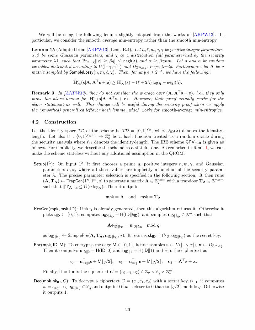
We will be using the following lemma slightly adapted from the works of [AKPW13]. Inparticular, we consider the smooth average min-entropy rather than the smooth min-entropy.

Lemma 15 (Adapted from [AKPW13], Lem. B.4). Let n, `,m, q, γ be positive integer parameters,α, β be some Gaussian parameters, and χ be a distribution (all parameterized by the securityparameter λ), such that Prx←χ[|x| ≥ βq] ≤ negl(λ) and α ≥ βγnm. Let s and e be randomvariables distributed according to U([−γ, γ]n) and DZm,αq, respectively. Furthermore, let A be amatrix sampled by SampleLossy(n,m, `, χ). Then, for any ε ≥ 2−λ, we have the following:.

Hε∞(s|A,A>s + e) ≥ H∞(s)− (`+ 2λ) log q − negl(λ).

Remark 3. In [AKPW13], they do not consider the average over (A,A>s + e), i.e., they onlyprove the above lemma for Hε

∞(s|A,A>s + e). However, their proof actually works for theabove statement as well. This change will be useful during the security proof when we applythe (smoothed) generalized leftover hash lemma, which works for smooth-average min-entropies.

4.2 Construction

Let the identity space ID of the scheme be ID = 0, 1`ID , where `ID(λ) denotes the identity-length. Let also H : 0, 1`ID+1 → Znq be a hash function treated as a random oracle duringthe security analysis where `ID denotes the identity-length. The IBE scheme GPVmult is given asfollows. For simplicity, we describe the scheme as a stateful one. As remarked in Rem. 1, we canmake the scheme stateless without any additional assumption in the QROM.

Setup(1λ): On input 1λ, it first chooses a prime q, positive integers n,m, γ, and Gaussianparameters α, σ, where all these values are implicitly a function of the security param-eter λ. The precise parameter selection is specified in the following section. It then runs(A,TA)← TrapGen(1n, 1m, q) to generate a matrix A ∈ Zn×mq with a trapdoor TA ∈ Zm×msuch that ‖TA‖GS ≤ O(n log q). Then it outputs

mpk = A and msk = TA

KeyGen(mpk,msk, ID): If skID is already generated, then this algorithm returns it. Otherwise itpicks bID ← 0, 1, computes uID‖bID = H(ID‖bID), and samples eID‖bID ∈ Zm such that

AeID‖bID = uID‖bID mod q

as eID‖bID ← SamplePre(A,TA,uID‖bID , σ). It returns skID = (bID, eID‖bID) as the secret key.

Enc(mpk, ID,M): To encrypt a message M ∈ 0, 1, it first samples s← U([−γ, γ]), x← DZm,αq.Then it computes uID‖0 = H(ID‖0) and uID‖1 = H(ID‖1) and sets the ciphertext as

c0 = u>ID‖0s + Mbq/2e, c1 = u>ID‖1s + Mbq/2e, c2 = A>s + x.

Finally, it outputs the ciphertext C = (c0, c1, c2) ∈ Zq × Zq × Zmq .

Dec(mpk, skID, C): To decrypt a ciphertext C = (c0, c1, c2) with a secret key skID, it computesw = cbID−c>2 eID‖bID ∈ Zq and outputs 0 if w is closer to 0 than to bq/2e modulo q. Otherwiseit outputs 1.

26

4.3 Correctness and Parameter Selection

The following shows correctness of the above IBE scheme.

Lemma 16 (Correctness). Suppose the parameters q, σ, and α are such that

σ > ‖TA‖GS ·√

log(2m+ 4)/π, α < 1/4σm.

Let eID‖bID ← KeyGen(A,TA, ID), C ← Enc(A, ID′,M ∈ 0, 1) and M′ ← Dec(A, eID‖bID , C). IfID = ID′, then with overwhelming probability we have M′ = M.

Proof. When the Dec algorithm operates as specified, we have

w = cbID − e>ID‖bIDc2 = Mbq/2e+ e>ID‖bIDx︸ ︷︷ ︸error term

.

By Lem. 8 and the condition posed on the choice of σ, we have that the distribution of eID‖bID is

2−Ω(n) close to DΛ⊥uID‖bID(A),σ. Therefore, by Lem. 5, we have ‖x‖ ≤ αq

√m, and ‖eID‖bID‖ ≤ σ ·

√m

except for 2−Ω(n) probability. Then, the error term is bounded by

|e>ID‖bIDx| ≤ ‖eID‖bID‖ · ‖x‖ ≤ αqσm.

Hence, for the error term to have absolute value less than q/4, it suffices to choose q and α as inthe statement of the lemma.

Parameter Selection. For the system to satisfy correctness and make the security proof work,we need the following restrictions. Note that we will prove the security of the scheme underLWE`,m,q,χm , where ` is specified in the following.

- The error term is less than q/4 (i.e., α < 1/4mσ by Lem. 16)

- TrapGen operates properly (i.e., m > 3n log q by Lem. 8)

- Samplable from DΛ⊥uID‖bID(A),σ (i.e., σ > ‖TA‖GS ·

√log(2m+ 4)/π = O(

√n logm log q) by

Lem. 8),

- LWE`,n,q,χ is hard so that we can use the lossy mode in the proof by Lem. 14 (i.e., χ = DZ,2√`),

- σ is sufficiently large so that we can apply Lem. 4 (i.e., σ >√n+ logm),

- we can apply to Lem. 15 in the proof (i.e., α > βγnm for β such that Prx←χ[|x| ≥ βq] ≤ negl(λ)),

- we can apply the generalized leftover hash lemma (Lem. 13) in the proof (i.e., n log(2γ)− (`+3λ) log q ≥ log q + Ω(n)).

To satisfy these requirements, for example, we can set the parameters `, n,m, q, σ, α, β, γ as follows:

n = 25`, m = n1+κ, σ = n0.5+κ, q = 5n5.5+3κ,

αq = n4+κ, βq = n, γ = n,

where κ > 0 is a constant that can be set arbitrarily small. To withstand attacks running in time2λ, we may set ` = Ω(λ). In the above, we round up m to the nearest integer and q to the nearestlargest prime. As the case with the single-challenge setting, if we make the more aggressive choiceof using the negligible notion 2−ω(log λ), we will be able to obtain better parameter selections.

27

4.4 Security Proof in ROM

We can (almost) tightly prove the security of our IBE scheme GPVmult both in the classical ROMand QROM settings. The following theorem addresses the security of GPVmult in the classicalROM setting.

Theorem 3. The IBE scheme GPVmult is adaptively-anonymous multi-challenge secure assumingthe hardness of LWE`,m,q,χ in the random oracle model, where χ = DZ,αq. Namely, for any classicalPPT adversary A making at most QH queries to H, Qch challenge queries, and QID secret keyqueries, there exists a classical PPT algorithm B such that

AdvIBEA,GPVmult(λ) ≤ 3n · Adv

LWE`,m,q,DZ,αqB (λ) + (QH +QID +Qch) · 2−Ω(n)

andTime(B) = Time(A) + (QH +QID +Qch) · poly(λ).

Proof of Theorem 3. Let CTSam(mpk) be an algorithm that outputs (c0, c1, c2) such that c0 ← Zq,c1 ← Zq, and c2 = A>s + x for s ← U([−γ, γ]) and x ← DZm,αq. Let also A be a classical PPTadversary that attacks the (multi-challenge) adaptively-anonymous security of the IBE scheme.Without loss of generality, we make some simplifying assumptions on A. First, we assume thatwhenever A queries a secret key or asks for a challenge ciphertext, ID‖0 and ID‖1 for the corre-sponding ID has already been queried to the random oracle H. We also assume that whenever Aqueries H on input ID‖b, it also queries H on input ID‖b as well. Furthermore, we assume thatA makes the same query for the random oracle or secret key oracle at most once. We show thesecurity of the scheme via the following games. In each game, we define Xi as the event that theadversary A wins in Gamei.

Game0 : This is the real security game. At the beginning of the game, (A,TA)← TrapGen(1n, 1m, q)is run and the adversary A is given A. The challenger then samples coin ← 0, 1 and keeps itsecret. During the game, A may make random oracle queries, secret key queries, and challengequeries. These queries are handled as follows:

• When A queries the random oracle H on ID‖0 and ID‖1, the challenger samples uID‖0 ← Znqand uID‖1 ← Znq and returns uID‖0 and uID‖1.

• When A queries a secret key for ID, the challenger first computes bID ← 0, 1 and returnseID‖bID = SamplePre(A,TA,uID‖bID , σ) to A where uID‖bID is the vector chosen during thesimulation of the random oracle.

• When the adversary makes the challenge query for ID∗ and a message M∗, the challengerreturns (c0, c1, c2) ← Encrypt(mpk, ID∗,M∗) if coin = 0 and (c0, c1, c2) ← CTSam(mpk) ifcoin = 1. It then returns C∗ = (c0, c1, c2) to A.

At the end of the game, A outputs a guess coin for coin. Finally, the challenger outputs coin. Bydefinition, we have

∣∣Pr[X0]− 12

∣∣ =∣∣Pr[coin− coin]− 1

2

∣∣ = AdvIBEA,GPVmult(λ).

Game1 : In this game, we change the game so that bID is chosen when A queries the random oracleH on input ID‖0 and ID‖1 rather than when A queries a secret key for ID. It is clear that this isonly a conceptual change and we have Pr[X0] = Pr[X1].

Game2 : In this game, we change the way the random oracle queries to H are answered. WhenA queries H on inputs ID‖0 and ID‖1, the challenger first samples bID ← 0, 1 as specified

28

in the previous game. Then, it generates a pair (uID‖bID , eID‖bID) by first sampling eID‖bID ←DZm,σ and setting uID‖bID = AeID‖bID . It also samples uID‖bID ← Znq . Then it locally stores

the tuples (ID‖bID,uID‖bID ,⊥) and (ID‖bID,uID‖bID ,⊥), and returns uID‖0 and uID‖1 to A. Here,we remark that when A makes a secret key query for ID, the challenger returns e′ID‖bID ←SamplePre(A,TA,uID‖bID , σ), which is independent from eID‖bID that was generated in the sim-ulation of the random oracle H on input ID‖0 and ID‖1. Note that in this game, we onlychange the distribution of uID‖bID for each identity. Due to Lem. 4, the distribution of uID‖bIDin Game2 is 2−Ω(n)-close to that of Game1 except for 2−Ω(n) fraction of A since we chooseσ >

√n+ logm. Therefore, the statistical distance between the view of A in Game1 and Game2

is 2−Ω(n) +QH · 2−Ω(n) < QH · 2−Ω(n). Therefore, we have∣∣Pr[X1]− Pr[X2]

∣∣ = QH · 2−Ω(n).

Game3 : In this game, we change the way secret key queries are answered. By the end of thisgame, the challenger will no longer require the trapdoor TA to generate the secret keys. When Aqueries H on ID‖0 and ID‖1, the challenger generates a pair (uID‖bID , eID‖bID) and uID‖bID as in the

previous game. Then it locally stores the tuple (ID‖bID,uID‖bID , eID‖bID) and (ID‖bID,uID‖bID ,⊥),and returns uID‖bID and uID‖bID to A. When A queries a secret key for ID, the challenger retrievesthe unique tuple (ID‖bID,uID‖bID , eID‖bID) from local storage and returns eID‖bID . For any fixed

uID‖bID ∈ Znq , let e(2)ID‖bID and e

(3)ID‖bID be random variables that are distributed according to the

distributions of skID‖bID conditioning on H(ID‖bID) = uID‖bID in Game2 and Game3, respectively.

Due to Lem. 8, we have ∆(e(2)ID‖bID , DΛ⊥uID‖bID

(A),σ) ≤ 2−Ω(n). On the other hand, due to Lem. 4, we

have ∆(e(3)ID‖bID , DΛ⊥uID‖bID

(A),σ) ≤ 2−Ω(n). Since A obtains at most QID user secret keys, we have∣∣Pr[X2]− Pr[X3]∣∣ = QID · 2−Ω(n).

Game4 : In this game, we change the way the matrix A is generated. Concretely, the challengerchooses A← Zn×mq without generating the associated trapdoor TA. By Lem. 8, this makes only

2−Ω(n)-statistical difference. Since the challenger can answer all the secret key queries withoutthe trapdoor due to the change we made in the previous game, the view of A is altered onlynegligibly. Therefore, we have

∣∣Pr[X3]− Pr[X4]∣∣ = 2−Ω(n).

Game5 : In this game, we change A to the lossy mode (See Lem. 15). We claim that∣∣Pr[X4] −

Pr[X5]∣∣ is negligible assuming the hardness of the LWE`,m,q,DZ,αq problem. To show this, we use

A to construct an adversary B′ that distinguishes random A from that in lossy mode. This canbe done by a straightforward reduction since B′ does not require the master secret key TA tosimulate the game due to the modification we made in Game3. We therefore by Lem. 14 conclude

that there exists B such that∣∣Pr[X4]− Pr[X5]

∣∣ = n · AdvLWE`,m,q,DZ,αqB (λ).

Game6 : In this game, we change the way the challenge ciphertexts are generated. Recall thatby our assumption, A makes queries for H on inputs ID∗‖0 and ID∗‖1 before making a challengequery for identity ID∗. When A makes a challenge query for (ID∗,M∗) it samples a ciphertext asC∗ ← CTSam(mpk) and returns C∗ to A if coin = 1. If coin = 0, it generates the ciphertext as

cbID∗ = u>ID∗‖bID∗ s + M∗bq/2e, cbID∗ ← Zq, c2 = A>s + x.

for s← U([−γ, γ]), where bID∗ is generated when the hash queries for ID∗‖0 and ID∗‖1 were made.It then rearranges the terms if necessary and returns (c0, c1, c2) to A.

We argue that the view of A is statistically close to that in the previous game. To prove this,we make a hybrid argument over all the challenge ciphertexts and change cbID∗ to be random one-by-one (when coin = 0). To conclude, it suffices to show that each ciphertext cbID∗ is distributed

29

2−Ω(n) close to the uniform distribution over Zq. Specifically, for each ciphertext, for any ε′ = 2−λ,we have

Hε′∞(s|A, cbID∗ , c2) ≥ Hε′

∞(s|A, c2)− log q

≥ H∞(s)− (`+ 2λ+ 1) log q − negl(λ)

= n log(2γ)− (`+ 3λ) log q

≥ log q + Ω(n)

where the first inequality follows by applying Lem. 12 with Z = Zq and ε = 0, the secondinequality follows from Lem. 15, and the last inequality follows from our parameter choice. Thisimplies that ∆(uID∗‖bID∗ ,u

>ID∗‖bID∗

s, |A, cbID∗ , c2) ≤ 2−Ω(n) for uID∗‖bID∗ ← Znq by Lem. 13 together

with Fact 1. Therefore, we have∣∣Pr[X5]− Pr[X6]

∣∣ = Qch · 2−Ω(n).

From Game7 to Game10 in the following, we undo the changes we added from Game2 to Game5.

Game7 : In this game, A is sampled as A ← Zn×mq . Similarly to the change from Game 4 to

Game 5, there exists B such that we have∣∣Pr[X6]− Pr[X7]

∣∣ = n · AdvLWE`,m,q,DZ,αqB (λ).

Game8 : In this game, A is sampled with a trapdoor as (A,TA)← TrapGen(1n, 1m, q). Similarlyto the change from Game 3 to Game 4, we have

∣∣Pr[X7]− Pr[X8]∣∣ = 2−Ω(n).

Game9 : In this game, we change the way secret key queries are answered. When A makes a secretkey query for ID, the challenger returns e′ID‖bID ← SamplePre(A,TA,uID‖bID , σ), where bID and uID

are chosen when random oracle queries on ID‖0 and ID‖1 are made. Similarly to the change fromGame 2 to Game 3, we have

∣∣Pr[X8]− Pr[X9]∣∣ = QH · 2−Ω(n).

Game10 : In this game, we change the way the random oracle queries to H are answered. When Aqueries the random oracle on ID‖0 and ID‖1, the challenger samples uID‖0,uID‖1 ← Znq and locallystores the tuples (ID‖0,uID‖0,⊥) and (ID‖1,uID‖1,⊥), and returns uID‖0 and uID‖1 to A. TheseuID‖0 and uID‖1 are also used when answering the secret key queries. Similarly to the change from

Game 1 to Game 2, we have∣∣Pr[X10]− Pr[X9]

∣∣ = QH · 2−Ω(n).

Because of the changes we introduced in Game7 to Game10, we can add the following change.

Game11 : In this game, we change the way the challenge ciphertexts are generated. When Amakes a challenge query for (ID∗,M∗), it returns a random ciphertext if coin = 1. If coin = 0, itgenerates the ciphertext as

cbID∗ ← Zq, cbID∗ = u>ID∗‖bID∗ s + M∗bq/2e, c2 = A>s + x.

for s← Znq , where bID∗ is generated when the hash queries for ID∗‖0 and ID∗‖1 were made. It thenrearranges the terms if necessary and returns (c0, c1, c2) to A. We claim that this change is onlyconceptual. Note that the distribution of the ciphertexts in this game corresponds to that in theprevious game, if we were to flip the value of bID∗ for every challenge identity ID∗. However, sinceA never makes a secret key query for ID∗ and uID∗‖0 and uID∗‖1 are sampled from exactly the samedistribution, the value of bID∗ is information theoretically hidden from A. This implies that thedistributions are the same in this and the previous game. Therefore, we have Pr[X11] = Pr[X10].

Game12 : In this game, we further change the way the challenge ciphertexts are generated. WhenA makes a challenge query for (ID∗,M∗), it returns a ciphertext sampled from CTSam(mpk) ifcoin = 1. If coin = 0, it generates the ciphertext as

cbID∗ ← Zq, cbID∗ ← Zq, c2 = A>s + x.

30

for s ← Znq and x ← DZm,αq. It then returns (c0, c1, c2) to A. We claim that the change isunnoticed by A assuming the LWE assumption. This can be shown by adding changes to Game11

that are almost the same as those we introduced from Game2 to Game6. The only difference isthat cbID∗ is always sampled as cbID∗ ← Zq here. By the similar analysis, there exists B such that

we have |Pr[X11]− Pr[X12]| ≤ n · AdvLWE`,m,q,DZ,αqB′ (λ) + (QH +QID +Qch) · 2−n.

Finally, we observe that the challenge ciphertexts are sampled from CTSam(mpk) regardlessof whether coin = 0 or 1. Therefore, we have Pr[X12] = 1/2. Putting things together, the theoremreadily follows.

4.5 Security Proof in QROM

As we explained in the introduction, our analysis in the ROM can be easily extended to the QROMsetting. Specifically, we prove the following theorem that addresses the security of GPVmult in theQROM.

Theorem 4. The IBE scheme GPVmult is adaptively-anonymous multi-challenge secure assumingthe hardness of LWE`,m,q,χ in the quantum random oracle model, where χ = DZ,αq. Namely, forany quantum polynomial time adversary A making at most QH quantum random oracle queries,Qch challenge queries, and QID secret key queries, there exists a quantum polynomial time algo-rithm B making at most 3QH + 2QID + 6Qch quantum random oracle queries such that

AdvIBEA,GPVmult(λ) ≤ 3n · Adv

LWE`,m,q,DZ,αqB,QRO`ID+2,max`r,(blog qc+n)×n

(λ) + (QH +QID +Qch) · 2−Ω(n)

andTime(B) = Time(A) + (QH +QID +Qch) · poly(λ)

where `r denotes the length of the randomness for SampleZ.

Proof of Theorem 4. Let CTSam(mpk) be an algorithm that outputs (c0, c1, c2) such that c0 ← Zq,c1 ← Zq, and c2 = A>s + x for s ← U([−γ, γ]) and x ← DZm,αq. Let also A be a quantumadversary that attacks the (multi-challenge) adaptively-anonymous security of the IBE scheme.Without loss of generality, we can assume that A makes secret key queries on the same identityat most once.

Game0 : This is the real security game. At the beginning of the game, the challenger chooses arandom function H ← Func(0, 1`ID+1,Znq ), which is used to simulate the random oracle. Thechallenger generates (A,TA) ← TrapGen(1n, 1m, q) and the adversary A is given A. The chal-lenger then samples coin← 0, 1 and keeps it secret. During the game, A may make (quantum)random oracle queries, secret key queries, and challenge queries. These queries are handled asfollows:

• When A makes a random oracle query on a quantum state∑

ID,b,y αID,b,y |ID‖b〉 |y〉, then thechallenger returns

∑ID,b,y αID,b,y |ID‖b〉 |H(ID‖b)⊕ y〉.

• When A makes a secret key query on ID, the challenger first chooses bID ← 0, 1, computesuID‖bID = H(ID‖bID), and returns eID‖bID = SamplePre(A,TA,uID‖bID , σ) to A.

• When A makes the challenge query for ID∗ and a message M∗, the challenger returns(c0, c1, c2) ← Encrypt(mpk, ID∗,M∗) if coin = 0 and (c0, c1, c2) ← CTSam(mpk) if coin = 1.It then returns C∗ = (c0, c1, c2) to A.

31

At the end of the game, A outputs a guess coin for coin. Finally, the challenger outputs coin. Bydefinition, we have

∣∣Pr[X0]− 12

∣∣ =∣∣Pr[coin− coin]− 1

2

∣∣ = AdvIBEA,GPVmult(λ).

Game1 : In this game, we change the way bID is chosen in simulations of secret key queries. Namely,in this game, the challenger first picks a random function H′ ← Func(0, 1`ID , 0, 1). When Amakes a secret key query ID, the challenger uses bID = H′(ID) instead of randomly choosing it.We remark that an oracle access to H′ is not given to A. Since H′(ID) is an independently anduniformly random bit for all ID, we have Pr[X0] = Pr[X1].

Game2 : In this game, we change the way the random oracle H is simulated. Namely, thechallenger first chooses additional random functions H0 ← Func(0, 1`ID , 0, 1`r) and H1 ←Func(0, 1`ID , 0, 1(blog qc+n)×n). Let ι : 0, 1(blog qc+n)×n → Znq denote a natural embedding

function. More precisely, it is given (a1, ..., an) ∈ 0, 1(blog qc+n)×n as an input, and outputs (a1

mod q, ..., an mod q)T where ai denotes a positive integer whose binary representation is ai. Itis easy to see that if we sample (a1, ..., an) ← 0, 1(blog qc+n)×n, then the statistical distance be-tween the distribution of ι(a1, ..., an) and the uniform distribution over Znq is 2−Ω(n). Then thechallenger defines H as follows:

H(ID‖b) :=

AeID‖b If b = H′(ID)

ι(H1(ID)) Otherwise(4)

where eID‖b := SampleZ(σ; H0(ID)). We remark that oracle accesses to H0 and H1 are not givento A. For any fixed ID, for the case of b 6= H′(ID), the distribution of H(ID‖b) is identical forall ID and its statistical distance from the uniform distribution is 2−Ω(n) as remarked above.For the case of b = H′(ID), the distribution of H(ID‖b) is identical for all ID and its statis-tical distance from the uniform distribution is 2−Ω(n) for all but 2−Ω(n) fraction of A due toLem. 4 since we choose σ >

√n+ logm. Then due to Lem. 2, we have

∣∣Pr[X1] − Pr[X2]∣∣ =

2−Ω(n) + 4Q2H

√2−Ω(n) + 4Q2

H

√2−Ω(n) = Q2

H · 2−Ω(n).

Game3 : In this game, we change the way secret key queries are answered. By the end of thisgame, the challenger will no longer require the trapdoor TA to generate the secret keys. WhenA queries a secret key for ID, the challenger returns (bID, eID) where bID = H′(ID) and eID‖bID :=

SampleZ(σ; H0(ID)). Since bID is unchanged from the previous game, we only have to provethat the distribution of eID‖bID differs negligibly from that in the previous game. For any fixed

uID‖bID ∈ Znq , let e(2)ID‖bID and e

(3)ID‖bID be random variables that are distributed according to the

distributions of eID‖bID conditioning on H(ID‖bID) = uID‖bID in Game2 and Game3, respectively.

Due to Lem. 8, we have ∆(e(2)ID‖bID , DΛ⊥uID‖bID

(A),σ) ≤ 2−Ω(n). On the other hand, due to Lem. 4,

we have ∆(e(3)ID‖bID , DΛ⊥uID‖bID

(A),σ) ≤ 2−Ω(n). Since A obtains at most QID user secret keys eID, we

have∣∣Pr[X2]− Pr[X3]

∣∣ = QID · 2−Ω(n).

Game4 : In this game, we change the way the matrix A is generated. Concretely, the challengerchooses A← Zn×mq without generating the associated trapdoor TA. By Lem. 8, the distribution

of A differs at most by 2−Ω(n). Since the challenger can answer all the secret key queries withoutthe trapdoor due to the change we made in the previous game, the view of A is altered only by2−Ω(n). Therefore, we have

∣∣Pr[X3]− Pr[X4]∣∣ = 2−Ω(n).

Game5 : In this game, we change A to the lossy mode (See Lem. 15). We claim that∣∣Pr[X4] −

Pr[X5]∣∣ is negligible assuming the hardness of the LWE`,n,q,DZ,αq problem relative to a quantum

32

random oracle |H〉 : 0, 1`ID+2 → 0, 1max`r,(blog qc+n)×n. For this purpose, we construct analgorithm B′ that distinguishes uniform A and that in the lossy mode relative to |H〉. As remarkedin Sec. 2.1, we can implement three independent quantum random oracles |H′〉 : 0, 1`ID → 0, 1,|H0〉 : 0, 1`ID → 0, 1`r , and |H1〉 : 0, 1`ID → 0, 1(blog qc+n)×n by using |H〉. Therefore weassume that B′ can access to three random oracles |H′〉, |H0〉 and |H1〉.B′ is given a matrix A, and its task is to distinguish whether A← Znq or A← SampleLossy(n,m, `, χ).

First, we remark that B′ can simulate the quantum random oracle |H〉 by using its own randomoracles |H′〉, |H0〉 and |H1〉 because |H〉 is programmed based on these three oracles by the modifi-cation made in Game2. B′ sets the master public key to be the LWE matrix A. Note that unlikethe real IBE scheme, B′ does not require the master secret key TA due to the modification wemade in Game4. Namely, when A queries ID for the secret key oracle, B′ just returns (bID, eID‖bID)

where bID = H′(ID) and eID‖bID := SampleZ(σ; H0(ID)). When A makes a challenge query for(ID∗,M∗), it samples a ciphertext as C∗ ← CTSam(mpk) if coin = 1, and honestly generates aciphertext as C∗ ← Encrypt(mpk, ID∗,M∗) if coin = 0, and returns C∗ to A. At the end of the

game, A outputs coin. Finally, B outputs 1 if coin = coin and 0 otherwise.It can be seen that if A ← Zn×mq the view of the adversary corresponds to Game5, and if

A ← SampleLossy(n,m, `, χ) the view of the adversary corresponds to Game6. Therefore we canbound

∣∣Pr[X5] − Pr[X6]∣∣ by the distinguishing advantage of B′, which makes at most 3QH +

2QID + 6Qch quantum random oracle queries. As for the running time, we have Time(B′) =Time(A) + (QH + QID + Qch) · poly(λ) since all B′ has to do is to run A once plus to computesome additional computations that can be done in a fixed polynomial time whenever A makes anyquery. Then by Lem. 14 we conclude that there exists B such that we have

∣∣Pr[X4]− Pr[X5]∣∣ =

n · AdvLWE`,m,q,DZ,αqB,QRO`ID+2,max`r,(blog qc+n)×n

(λ) and the running time of B is almost the same as that of B′.

Game6 : In this game, we change the way the challenge ciphertexts are generated. When A makesa challenge query for (ID∗,M∗), it samples a ciphertext as C∗ ← CTSam(mpk) and returns C∗ toA if coin = 1. If coin = 0, it generates the ciphertext as

cbID∗ = u>ID∗‖bID∗ s + M∗bq/2e, cbID∗ ← Zq, c2 = A>s + x.

for s ← U([−γ, γ]), where bID∗ = H′(ID∗). It then rearranges the terms if necessary and returns(c0, c1, c2) to A.

We argue that the view of A is statistically close to that in the previous game. To prove this,we make a hybrid argument over all the challenge ciphertexts and change cbID∗ to be random one-by-one (when coin = 0). To conclude, it suffices to show that each ciphertext cbID∗ is distributed

2−Ω(n) close to the uniform distribution over Zq. Specifically, for each ciphertext, for any ε′ = 2−λ,we have

Hε′∞(s|A, cbID∗ , c2) ≥ Hε′

∞(s|A, c2)− log q

≥ H∞(s)− (`+ 2λ+ 1) log q − negl(λ)

= n log(2γ)− (`+ 3λ) log q

≥ log q + Ω(n)

where the first inequality follows by applying Lem. 12 with Z = Zq and ε = 0, the secondinequality follows from Lem. 15, and the last inequality follows from our parameter choice. Thisimplies that ∆(uID∗‖bID∗ ,u

>ID∗‖bID∗

s, |A, cbID∗ , c2) ≤ 2−Ω(n) for uID∗‖bID∗ ← Znq by Lem. 13 together

with Fact 1. Therefore, we have∣∣Pr[X5]− Pr[X6]

∣∣ = Qch · 2−Ω(n).

33

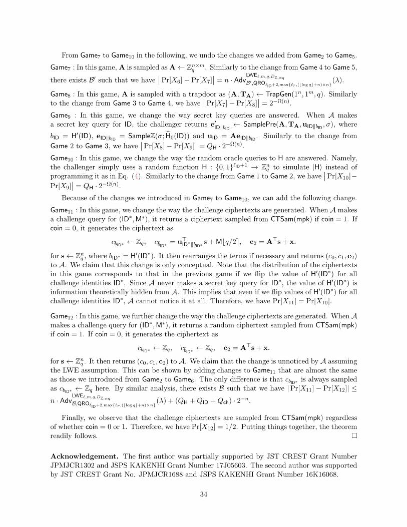
From Game7 to Game10 in the following, we undo the changes we added from Game2 to Game5.

Game7 : In this game, A is sampled as A← Zn×mq . Similarly to the change from Game 4 to Game 5,

there exists B′ such that we have∣∣Pr[X6]− Pr[X7]

∣∣ = n · AdvLWE`,m,q,DZ,αqB′,QRO`ID+2,max`r,(blog qc+n)×n

(λ).

Game8 : In this game, A is sampled with a trapdoor as (A,TA)← TrapGen(1n, 1m, q). Similarlyto the change from Game 3 to Game 4, we have

∣∣Pr[X7]− Pr[X8]∣∣ = 2−Ω(n).

Game9 : In this game, we change the way secret key queries are answered. When A makesa secret key query for ID, the challenger returns e′ID‖bID ← SamplePre(A,TA,uID‖bID , σ), where

bID = H′(ID), eID‖bID = SampleZ(σ; H0(ID)) and uID = AeID‖bID . Similarly to the change from

Game 2 to Game 3, we have∣∣Pr[X8]− Pr[X9]

∣∣ = QH · 2−Ω(n).

Game10 : In this game, we change the way the random oracle queries to H are answered. Namely,the challenger simply uses a random function H : 0, 1`ID+1 → Znq to simulate |H〉 instead ofprogramming it as in Eq. (4). Similarly to the change from Game 1 to Game 2, we have

∣∣Pr[X10]−Pr[X9]

∣∣ = QH · 2−Ω(n).

Because of the changes we introduced in Game7 to Game10, we can add the following change.

Game11 : In this game, we change the way the challenge ciphertexts are generated. When A makesa challenge query for (ID∗,M∗), it returns a ciphertext sampled from CTSam(mpk) if coin = 1. Ifcoin = 0, it generates the ciphertext as

cbID∗ ← Zq, cbID∗ = u>ID∗‖bID∗ s + Mbq/2e, c2 = A>s + x.

for s← Znq , where bID∗ = H′(ID∗). It then rearranges the terms if necessary and returns (c0, c1, c2)to A. We claim that this change is only conceptual. Note that the distribution of the ciphertextsin this game corresponds to that in the previous game if we flip the value of H′(ID∗) for allchallenge identities ID∗. Since A never makes a secret key query for ID∗, the value of H′(ID∗) isinformation theoretically hidden from A. This implies that even if we flip values of H′(ID∗) for allchallenge identities ID∗, A cannot notice it at all. Therefore, we have Pr[X11] = Pr[X10].

Game12 : In this game, we further change the way the challenge ciphertexts are generated. WhenAmakes a challenge query for (ID∗,M∗), it returns a random ciphertext sampled from CTSam(mpk)if coin = 1. If coin = 0, it generates the ciphertext as

cbID∗ ← Zq, cbID∗ ← Zq, c2 = A>s + x.

for s← Znq . It then returns (c0, c1, c2) to A. We claim that the change is unnoticed by A assumingthe LWE assumption. This can be shown by adding changes to Game11 that are almost the sameas those we introduced from Game2 to Game6. The only difference is that cbID∗ is always sampledas cbID∗ ← Zq here. By similar analysis, there exists B such that we have |Pr[X11] − Pr[X12]| ≤n · Adv

LWE`,m,q,DZ,αqB,QRO`ID+2,max`r,(blog qc+n)×n

(λ) + (QH +QID +Qch) · 2−n.

Finally, we observe that the challenge ciphertexts are sampled from CTSam(mpk) regardlessof whether coin = 0 or 1. Therefore, we have Pr[X12] = 1/2. Putting things together, the theoremreadily follows.

Acknowledgement. The first author was partially supported by JST CREST Grant NumberJPMJCR1302 and JSPS KAKENHI Grant Number 17J05603. The second author was supportedby JST CREST Grant No. JPMJCR1688 and JSPS KAKENHI Grant Number 16K16068.

34

References

[ABB10] Shweta Agrawal, Dan Boneh, and Xavier Boyen. Efficient lattice (h) ibe in thestandard model. In EUROCRYPT, pages 553–572. Springer, 2010. 6

[ABB+17] Erdem Alkim, Nina Bindel, Johannes A. Buchmann, Ozgur Dagdelen, EdwardEaton, Gus Gutoski, Juliane Kramer, and Filip Pawlega. Revisiting TESLA inthe quantum random oracle model. In PQCrypto, pages 143–162. Springer, 2017.10

[ACPS09] Benny Applebaum, David Cash, Chris Peikert, and Amit Sahai. Fast cryptographicprimitives and circular-secure encryption based on hard learning problems. InCRYPTO, pages 595–618. Springer, 2009. 8

[ADN+10] Joel Alwen, Yevgeniy Dodis, Moni Naor, Gil Segev, Shabsi Walfish, and DanielWichs. Public-key encryption in the bounded-retrieval model. In EUROCRYPT,pages 113–134. Springer, 2010. 8

[AHY15] Nuttapong Attrapadung, Goichiro Hanaoka, and Shota Yamada. A framework foridentity-based encryption with almost tight security. In ASIACRYPT, pages 521–549. Springer, 2015. 10

[AKPW13] Joel Alwen, Stephan Krenn, Krzysztof Pietrzak, and Daniel Wichs. Learning withrounding, revisited. In CRYPTO, pages 57–74. Springer, 2013. 7, 24, 25, 26

[ARU14] Andris Ambainis, Ansis Rosmanis, and Dominique Unruh. Quantum attacks onclassical proof systems: The hardness of quantum rewinding. In FOCS, pages 474–483. IEEE, 2014. 10

[BDF+11] Dan Boneh, Ozgur Dagdelen, Marc Fischlin, Anja Lehmann, Christian Schaffner,and Mark Zhandry. Random oracles in a quantum world. In Eurocrypt, pages41–69. Springer, 2011. 3, 9, 11, 15

[BDPMW16] Florian Bourse, Rafael Del Pino, Michele Minelli, and Hoeteck Wee. Fhe circuitprivacy almost for free. In CRYPTO, pages 62–89. Springer, 2016. 8

[BF01] Dan Boneh and Matt Franklin. Identity-based encryption from the weil pairing. InCRYPTO, pages 213–229. Springer, 2001. 10, 12

[BG14] Shi Bai and Steven D. Galbraith. An improved compression technique for signaturesbased on learning with errors. In CT-RSA, pages 28–47, 2014. 10

[BKPW12] Mihir Bellare, Eike Kiltz, Chris Peikert, and Brent Waters. Identity-based (lossy)trapdoor functions and applications. In EUROCRYPT, pages 228–245. Springer,2012. 7, 25

[BL16] Xavier Boyen and QinYi Li. Towards tightly secure lattice short signature andid-based encryption. In ASIACRYPT(2), pages 404–434. Springer, 2016. 10

[BL18] Xavier Boyen and Qinyi Li. Almost tight multi-instance multi-ciphertext identity-based encryption on lattices. In ACNS, pages 535–553. Springer, 2018. 10

35

[BLP+13] Zvika Brakerski, Adeline Langlois, Chris Peikert, Oded Regev, and Damien Stehle.Classical hardness of learning with errors. In STOC, pages 575–584, 2013. 14, 15

[BPR12] Abhishek Banerjee, Chris Peikert, and Alon Rosen. Pseudorandom functions andlattices. In EUROCRYPT, pages 719–737. Springer, 2012. 12

[BR93] Mihir Bellare and Phillip Rogaway. Random oracles are practical: A paradigm fordesigning efficient protocols. In CCS, pages 62–73. ACM, 1993. 3, 9

[CHK04] Ran Canetti, Shai Halevi, and Jonathan Katz. Chosen-ciphertext security fromidentity-based encryption. In EUROCRYPT, pages 207–222. Springer, 2004. 9

[CHKP10] David Cash, Dennis Hofheinz, Eike Kiltz, and Chris Peikert. Bonsai trees, or howto delegate a lattice basis. In EUROCRYPT, pages 523–552. Springer, 2010. 6

[Cor09] Jean-Sebastien Coron. A variant of boneh-franklin ibe with a tight reduction in therandom oracle model. Designs, Codes and Cryptography, 50(1):115–133, 2009. 10

[CS98] Ronald Cramer and Victor Shoup. A practical public key cryptosystem provably se-cure against adaptive chosen ciphertext attack. In CRYPTO, pages 13–25. Springer,1998. 6

[CW13] Jie Chen and Hoeteck Wee. Fully,(almost) tightly secure ibe and dual system groups.In CRYPTO, pages 435–460. Springer, 2013. 10

[DORS04] Yevgeniy Dodis, Rafail Ostrovsky, Leonid Reyzin, and Adam Smith. Fuzzy ex-tractors: How to generate strong keys from biometrics and other noisy data. InEUROCRYPT, pages 523–540. Springer, 2004. 24, 25

[GDCC16] Junqing Gong, Xiaolei Dong, Jie Chen, and Zhenfu Cao. Efficient ibe with tightreduction to standard assumption in the multi-challenge setting. In ASIACRYPT,pages 624–654. Springer, 2016. 10

[Gen06] Craig Gentry. Practical identity-based encryption without random oracles. InEUROCRYPT, pages 445–464. Springer, 2006. 6

[GGM86] Oded Goldreich, Shafi Goldwasser, and Silvio Micali. How to construct randomfunctions. J. ACM, 33(4):792–807, 1986. 12

[GKPV10] Shafi Goldwasser, Yael Kalai, Chris Peikert, and Vinod Vaikuntanathan. Robust-ness of the learning with errors assumption. ICS, pages 230–240, 2010. 7, 25

[Gol86] Oded Goldreich. Two remarks concerning the goldwasser-micali-rivest signaturescheme. In CRYPTO, pages 104–110. Springer, 1986. 13

[GPV08] Craig Gentry, Chris Peikert, and Vinod Vaikuntanathan. Trapdoors for hard latticesand new cryptographic constructions. In STOC, pages 197–206. ACM, 2008. 3, 4,5, 8, 9, 14, 16, 18

[GSW13] Craig Gentry, Amit Sahai, and Brent Waters. Homomorphic encryption from learn-ing with errors: Conceptually-simpler, asymptotically-faster, attribute-based. InCRYPTO, pages 75–92. Springer, 2013. 8

36

[HJ12] Dennis Hofheinz and Tibor Jager. Tightly secure signatures and public-key encryp-tion. In CRYPTO, pages 590–607. Springer, 2012. 4, 7

[HKS15] Dennis Hofheinz, Jessica Koch, and Christoph Striecks. Identity-based encryptionwith (almost) tight security in the multi-instance, multi-ciphertext setting. In PKC,pages 799–822. Springer, 2015. 10

[JZC+18] Haodong Jiang, Zhenfeng Zhang, Long Chen, Hong Wang, and Zhi Ma. Ind-cca-secure key encapsulation mechanism in the quantum random oracle model, revisited.In CRYPTO, pages 96–125. Springer, 2018. 10

[KLS18] Eike Kiltz, Vadim Lyubashevsky, and Christian Schaffner. A concrete treatment offiat-shamir signatures in the quantum random-oracle model. In EUROCRYPT III,pages 552–586. Springer, 2018. 10

[KW03] Jonathan Katz and Nan Wang. Efficiency improvements for signature schemeswith tight security reductions. In Computer and Communications Security, pages155–164. ACM, 2003. 8, 10, 24

[KY16] Shuichi Katsumata and Shota Yamada. Partitioning via non-linear polynomial func-tions: more compact ibes from ideal lattices and bilinear maps. In ASIACRYPT,pages 682–712. Springer, 2016. 6, 9, 14

[LSSS17] Benoıt Libert, Amin Sakzad, Damien Stehle, and Ron Steinfeld. All-but-many lossytrapdoor functions and selective opening chosen-ciphertext security from lwe. InCRYPTO, pages 332–364. Springer, 2017. 7, 25

[MP12] Daniele Micciancio and Chris Peikert. Trapdoors for lattices: Simpler, tighter,faster, smaller. In EUROCRYPT, pages 700–718. Springer, 2012. 14

[MR07] Daniele Micciancio and Oded Regev. Worst-case to average-case reductions basedon gaussian measures. SIAM J. Comput., 37(1):267–302, 2007. 14

[NC00] Michael A. Nielsen and Isaac L. Chuang. Quantum Computation and QuantumInformation. Cambridge University Press, 2000. 10

[Pei07] Chris Peikert. Limits on the hardness of lattice problems in ell p norms. InConference on Computational Complexity, pages 333–346. IEEE, 2007. 14

[Pei09] Chris Peikert. Public-key cryptosystems from the worst-case shortest vector prob-lem. In STOC, pages 333–342. ACM, 2009. 15

[Pei10] Chris Peikert. An efficient and parallel gaussian sampler for lattices. In CRYPTO,pages 80–97. Springer, 2010. 14

[PR06] Chris Peikert and Alon Rosen. Efficient collision-resistant hashing from worst-caseassumptions on cyclic lattices. In TCC, pages 145–166. Springer, 2006. 14

[Reg05] Oded Regev. On lattices, learning with errors, random linear codes, and cryptog-raphy. In STOC, pages 84–93. ACM Press, 2005. 3, 7, 14, 15

[Reg10] Oded Regev. The learning with errors problem. Invited survey in CCC, 2010. 7

37

[RW04] Renato Renner and Stefan Wolf. Smooth renyi entropy and applications. In In-ternational Symposium on Information Theory – ISIT, pages 233–233. IEEE, 2004.24

[Sho94] Peter W. Shor. Algorithms for quantum computation: Discrete logarithms andfactoring. In FOCS, pages 124–134. IEEE, 1994. 3

[SXY18] Tsunekazu Saito, Keita Xagawa, and Takashi Yamakawa. Tightly-secure key-encapsulation mechanism in the quantum random oracle model. In EUROCRYPTIII, pages 520–551. Springer, 2018. 9, 10, 12

[TU16] Ehsan Ebrahimi Targhi and Dominique Unruh. Post-quantum security of thefujisaki-okamoto and OAEP transforms. In TCC II, pages 192–216. Springer, 2016.10

[Unr14a] Dominique Unruh. Quantum position verification in the random oracle model. InCRYPTO II, pages 1–18. Springer, 2014. 10

[Unr14b] Dominique Unruh. Revocable quantum timed-release encryption. In EUROCRYPT,pages 129–146. Springer, 2014. 10

[Unr15] Dominique Unruh. Non-interactive zero-knowledge proofs in the quantum randomoracle model. In EUROCRYPT II, pages 755–784. Springer, 2015. 10

[Unr17] Dominique Unruh. Post-quantum security of fiat-shamir. In ASIACRYPT I, pages65–95. Springer, 2017. 10

[Wat05] Brent Waters. Efficient identity-based encryption without random oracles. In EU-ROCRYPT, pages 114–127. Springer, 2005. 6

[Zha12a] Mark Zhandry. How to construct quantum random functions. In FOCS, pages679–687. IEEE, 2012. 4, 9, 12

[Zha12b] Mark Zhandry. Secure identity-based encryption in the quantum random oraclemodel. In CRYPTO, pages 758–775. Springer, 2012. 3, 4, 5, 9, 10, 11, 21

38