Tightly Coupled Integrated Inertial and Real-Time-KinematicPositioning Approach Using Nonlinear Observer

Jakob M. Hansen1, Tor Arne Johansen1 and Thor I. Fossen1

Abstract— Tightly coupled integration of inertial measure-ments and raw global navigation satellite measurements usinga nonlinear observer is proposed for real-time-kinematic ap-plications. The position, linear velocity and attitude estimatesof a rover is aided by global pseudo-range and carrier-phasemeasurements from the rover and a base station. The tightintegration is achieved using a modular observer design, wherethe attitude observer with gyro bias estimate is based ona nonlinear complementary filter. Two translational motionobservers estimating position and linear velocity using single-or double-differenced range measurements, respectively, arepresented. The range measurements include pseudo-range andcarrier-phase measurements from the satellite constellation torover and base station, where the integer ambiguity resolutionis estimated as part of the nonlinear observer state vector. Thefeedback interconnection of the observer systems is shown tobe exponentially stable. The proposed observers are tested withan unmanned aerial vehicle simulator.

I. INTRODUCTION

Vehicle navigation is often based on data from InertialMeasurement Units (IMUs) supplying inertial informationsuch as acceleration and angular velocity of the vehicle.Integration of the measurements allows for estimation ofposition, linear velocity and attitude of the vehicle, whichcan be further enhanced by use of aiding sensors, e.g.a magnetometer or a Global Navigation Satellite System(GNSS) receiver.

One method for INS/GNSS integration is the looselycoupled architecture, where a kinematic model is used tointegrate INS to position while correcting it with GNSSposition data. Another approach is the tightly coupled ar-chitecture where range measurements from a GNSS systemis used instead of position estimates for aiding. The primarydifference between the loosely and tightly coupled systems isthat the GNSS measurements are moved from the position-domain to the range-domain, see [1].

The accuracy of GNSS measurements suffer from signaldisturbances e.g. in the ionosphere and troposphere wherethe signal path can be obstructed due to shifts in magneticfield or atmospheric density. These disturbances can, tosome extend, be modeled based on local and solar weatherforecasts. Using multi-frequency receivers it is possible toestimate and compensate for ionospheric delay, section 8.6in [2], however these receivers are presently not widely useddue to their high price. Another approach for counteringthe atmospheric disturbances is to utilize a dual receiver

1Centre for Autonomous Marine Operations and Systems, Departmentof Engineering Cybernetics, Norwegian University of Science and Technol-ogy, 7491 Trondheim, Norway (e-mail: jakob.mahler.hansen@itk.ntnu.no,tor.arne.johansen@itk.ntnu.no, thor.fossen@ntnu.no)

configuration, where two receivers are placed close to eachother obtaining GNSS measurements from the same satelliteconstellation. In this case environmental disturbances areconsidered to be the same for the two receivers. With aknown position of the reference receiver, often called basestation, and a short baseline to the rover (vehicle) the signaldisturbances can be canceled.

Using the raw measurements from the satellite receiver, i.e.carrier-phase, pseudo-range or Doppler frequency measure-ments, tight integration with the inertial measurements allowfor an increase in precision, e.g. [1]. Multiple approaches fortight integration using Kalman filters have been proposed.Potential enhancements for tightly coupled integration onsmall unmanned aerial vehicles (UAVs) are listed in [3]. AKalman filter method using GPS velocity estimates insteadof carrier-phase measurements is proposed in [4]. An ex-tended Kalman filter integrating pseudo-ranges and Dopplermeasurements with a low-cost inertial sensor is proposedin [5] for assisting the phase-lock-loop tracking. [6] usetime-differenced carrier-phase measurements to eliminate theambiguities. The time-differenced approach was also appliedin [7] where an attitude determination system was designedusing a Kalman filter and a single-receiver configuration. In[8] the advantages of augmenting precise point positioningwith inertial measurements in a dual-frequency receiverconfiguration is investigated. The Kalman filter is based onlinear approximation of the nonlinear measurement model,where a need for higher order accuracy was investigated in[9], but found to be negligible for tightly coupled systems.A comparative study of loosely, tightly and ultra-tightlycoupled systems was investigated by [10] using a wide rangeof inertial sensor grades, and the GIGET tool. A tightlycoupled system utilizing a GPS compass for effective integerambiguity search was investigated by [11], using a low-costmulti-antenna setup. In [12] a new and faster method forinteger ambiguity resolution is proposed, which is confirmedwith experimental measurements.

Integration of inertial measurements and global positionmeasurements have been researched extensively, tradition-ally in filters as the extended Kalman filter [1], [2], andrecently with nonlinear observers [13], [14]. The advan-tages of the nonlinear observers compared to the widelyused extended Kalman filter are the reduced computationalworkload, proven stability qualities and reduced need forlinearization of the system model. An advantage of usingraw satellite measurements is that the solution is no longerdependent of the unknown properties of the Kalman filter inthe GNSS receiver supplying position estimates.

2016 American Control Conference (ACC)Boston Marriott Copley PlaceJuly 6-8, 2016. Boston, MA, USA

978-1-4673-8681-4/$31.00 ©2016 AACC 5511

The main contributions of the present paper are two non-linear translational motion observers utilizing as injection theerror between measured and estimated single- and double-differenced range measurements from the satellite constel-lation to rover and base station. For the single-differencedmethod the receiver clock error needs to be estimated,whereas this term is canceled for the double-differencedapproach. Where various Kalman filters for tightly coupledintegration have been put forward, and several nonlinearobservers have been proposed for loosely coupled GNSS/INSintegration, tight integration using nonlinear observers hasonly recently been proposed, [15] and [16], [17], [18], [19].The motivation is reduced computational load and moretransparent conditions for stability and region of attraction.

The problem will be stated formally in Section II, followedby the Real-Time-Kinematic (RTK) positioning approach inSection III, introducing the raw GNSS measurements. InSection IV and V the nonlinear observers will be introduced,while Section VI presents the method used for integerambiguity resolution. In Section VII some implementationand time scale considerations are presented. A case study isconducted in Section VIII presenting data from a simulatedunmanned aerial vehicle (UAV). The paper is concluded inSection IX.

II. PROBLEM STATEMENT

The objective of this paper is to estimate position, linearvelocity and attitude (PVA) of a vehicle by tightly coupledintegration of inertial measurements in the Body frameaided by range measurements from satellites. The satel-lite measurements include pseudo-range and carrier-phasemeasurements, obtained from the satellite broadcasts. Thenonlinear observer is based on [15], with several extensionssuch that the position estimate is computed as a moving-baseline RTK solution with fixed or real valued integerambiguities and known base station position. The raw satel-lite signal measurements are obtained at two locations: astationary (or slightly moving) base station and a movingrover. Estimation of the rover PVA as well as the baseline,i.e. the vector (displacement) between rover and base station,are of interest. The coordinate frames used will be denotedwith b for Body-frame and e for Earth-Centered-Earth-Fixed-frame. Here the rover and base station will be signified bythe indicators r and s, respectively.

The kinematic model of the rover and base station aredescribed by:

per = ve

r , (1)ve

r =−2S(ωeie)v

er + f e +ge(pe

r), (2)

qeb =

12

qeb⊗ ω

bib−

12

ωeie⊗qe

b, (3)

bb = 0, (4)pe

s = 0, (5)

where per , ve

r and qeb denote the position, linear velocity

and attitude of the rover, with the attitude represented as aunit quaternion expressed in the Earth-Centered-Earth-Fixed(ECEF) frame. The base station position, pe

s , is assumed to

be constant (or, in practice slowly time-varying). The specificforce is denoted f e, while the gravitational vector, ge, isa function of the rover position. The angular velocity andassociated rate gyro bias are denoted; ωb

ib and bb, expressedin the Body-frame, while the angular velocity of the Earthwith respect to the Earth-Centered Inertial (ECI) frame isdenoted ωe

ie. The skew-symmetric matrix of a vector isdenoted S(·) (see (B.14)–(B.15) [2]), while the Hamiltonquaternion product is denoted ⊗. A real valued vector,x ∈R3, can be expressed as a quaternion with zero real partdenoted as x = [0;x].

A. Measurement Assumptions

Determining the position of a vehicle using RTK requirestwo receivers, separated by a baseline. The RTK principleis based on the assumption that the ionospheric and tro-pospheric disturbances for the two receivers are identical,thereby making it possible to cancel them out by sharing theobtained satellite data between the two receivers.

In the literature the carrier-phase measurements can befound with unit of meters or cycles. In the following ϕ willdenote the carrier-phase measurement in meters, with ϕ =λϕcycles being the conversion from cycles to meters, whereλ is the wavelength of the signal.

The range measurements from the ith satellite are:

ρri = ψ

ri +β

r + εri , (6)

ϕri = ψ

ri +Nr

i λ +βr + er

i , (7)

where ψri is the geometric range from the ith satellite to

the rover, i.e. ψri = ‖pe

r− pei ‖2. Nr

i is the integer ambiguity,β r is the receiver clock range error, er

i and εri are covering

systematic environmental errors arising from the ionosphereand troposphere. The receiver clock range error is expressedas, β := c∆c, with c being the wave propagation speed and ∆cbeing the clock bias, between satellite and receiver clocks. Inaddition, there are smaller errors such as receiver noise that isnot explicitly included. When expressing the measurementsat the base station the superscript r is substituted for s.

The environmental disturbances are the same for the basestation and rover receiver, er

i = esi = ei and εr

i = εsi = εi,

where the subscript denotes measurements from the ithsatellite. Effectively this requires the baseline between thetwo antennas to be less than 20 km, [1].

The following sensor measurements are assumed availablefrom the rover:

• Specific force as measured by an IMU, f bIMU = f b.

• Angular velocity with bias as measured by an IMU,ωb

ib,IMU = ωbib +bb.

• Magnetic field measurements from a magnetometer, mb.• Pseudo-ranges measurements from satellites, ρr

i .• Carrier-phase measurements from satellites, ϕr

i .

Furthermore, it is assumed that pseudo-range, ρsi , and carrier-

phase, ϕsi , measurements are available at the base station.

There should be m ≥ 5 common satellites available in thetwo constellations.

5512

The satellite positions are assumed known, which can besatisfied by obtaining the transmitted ephemeris data fromeach satellite.

The method can be easily extended to exploit range-rate(Doppler) measurements, which are not included here forsimplicity.

III. REAL-TIME-KINEMATICS POSITIONING

The single-differenced measurements between the roverand base station from the ith satellite can eliminate thecommon environmental errors:

∆ρi = ∆ψi +∆β , (8)∆ϕi = ∆ψi +∆Niλ +∆β , (9)

where ∆ρi := ρri − ρs

i , ∆ϕi := ϕri − ϕs

i , ∆N := Nri −Ns

i =[∆N1,∆N2, . . . ,∆Nm], ∆β := β r−β s, and ∆ψi := ψr

i −ψsi is

the geometric baseline between rover and base station.Elimination of the clock error ∆β can be achieved by

double-differencing the measurements using an additionalsatellite j at the same epoch:

∇∆ρi j = ∇∆ψi j, (10)∇∆ϕi j = ∇∆ψi j +∇∆Ni jλ , (11)

where ∇∆ρi j := ∆ρ j−∆ρi, ∇∆ψi j := ∆ψ j−∆ψi, ∇∆ϕi j :=∆ϕ j − ∆ϕi, and ∇∆Ni j := ∆N j − ∆Ni. It is vital that themeasurements from the two satellites at the two receivers aresimultaneous. If this is not the case the geometric distancebetween satellite and receiver will have changed betweenthe measurements making the differential measurements in-accurate. The receivers are assumed to log and time stampthe raw measurements simultaneously for all satellites in theconstellation with a fixed update rate of 1−10 Hz. Moreover,it is assumed that coinciding measurements can be found forthe two satellites at the two receivers.

In the following sections two nonlinear observers willbe introduced, based on the single- and double-differencedmeasurements. The nonlinear observer design consists oftwo parts: an attitude observer and a translational motionobserver.

IV. NONLINEAR OBSERVER - SINGLE-DIFFERENCED

Estimating the rover attitude represented as the rotationbetween ECEF- and Body-frame as well as the gyro biasis achieved by the nonlinear attitude observer given in [20],[15], [21]:

˙qeb =

12

qeb⊗(

ωbib,IMU −

¯bb + ¯σ)− 1

2ω

eie⊗ qe

b, (12)

˙bb = Proj(−kIσ ,‖bb‖2 ≤Mb), (13)

σ = k1vb1×R(qe

b)T ve

1 + k2vb2×R(qe

b)T ve

2, (14)

where Proj(·, ·) is the projection function limiting theestimate to a sphere with constant radius Mb. The magneticfield of the Earth is denoted me, while k1, k2 and kI arepositive constants chosen sufficiently large. The vectors vb

1and vb

2 are two vectors in the Body-frame with corresponding

vectors ve1 and ve

2 in the ECEF-frame. The vectors can beconsidered in various forms, but will here be:

vb1 =

f bIMU

‖ f bIMU‖2

,vb2 =

mb

‖mb‖2× vb

1,

ve1 =

f e

‖ f e‖2,ve

2 =me

‖me‖2× ve

1.

The specific force estimate is supplied by the translationalmotion observer, inspired by [15]:

˙per = ve

r +m

∑i=1

(K pρ

i eρ,i +K pϕ

i eϕ,i), (15)

˙ver =−2S(ωe

ie)ver + f e +ge(pe

r)

+m

∑i=1

(Kvρ

i eρ,i +Kvϕ

i eϕ,i),

(16)

ξ =−R(qeb)S(σ) f b

IMU +m

∑i=1

(Kξ ρ

i eρ,i +Kξ ϕ

i eϕ,i

), (17)

f e = R(qeb) f b

IMU +ξ , (18)

˙ps =m

∑i=1

(Ksρ

i eρ,i +Ksϕ

i eϕ,i), (19)

∆˙β =

m

∑i=1

(Kβρ

i eρ,i +Kβϕ

i eϕ,i

), (20)

∆˙N =

m

∑i=1

(KNρ

i eρ,i +KNϕ

i eϕ,i

). (21)

The clock error, ∆β , is assumed to be the same for allsatellites, i.e. ∆β ∈ R1. The receiver errors are assumed todominate the clock range error diminishing the need forindividual estimation for each satellite.

The single-differenced ambiguities, ∆N, are initiallytreated as real valued when estimated in (21), where SectionVI will describe how the estimates are fixed to integervalues for increased precision. The observer structure issimilar to [15], with altered injection terms and addition ofbase station position and integer ambiguity estimation. Theinjection terms are the errors in single-differenced pseudo-range and carrier-phase, defined as: eρ,i := ∆ρi − ∆ρi andeϕ,i := ∆ϕi−∆ϕi. The estimated terms are determined as:

∆ρi = ∆ψi +∆β , ∆ϕi = ∆ψi +∆Niλ +∆β , (22)

where the geometric range difference estimate is:

∆ψi = ‖ per− pe

i ‖2−‖ pes− pe

i ‖2.

The measurement errors can be expressed as:

eρ,i = ‖per− pe

i ‖2−‖ per− pe

i ‖2−‖pes− pe

i ‖2

+‖pes− pe

i ‖2 +∆β ,(23)

eϕ,i = eρ,i +∆Niλ . (24)

The state estimation error vector is introduced as, x =[pr, vr, f , ps,∆β ,∆N]T , with pr := pe

r − per , vr := ve

r − ver ,

f := f e− f e, ps := pes− pe

s , ∆β :=∆β−∆β , ∆N :=∆N−∆N,where ξ is replaced with f by combination of (17) and (18).The measurement errors are linearized leaving:

eρ,i =Cρ,ix+h.o.t., (25)eϕ,i =Cϕ,ix+h.o.t., (26)

5513

where the higher order terms (h.o.t.) are neglected inthe observer gain selection, [15]. The measurement matri-ces are given by their rows Cρ,i = [ci,0,0, ci,1,0m], andCϕ,i = [ci,0,0, ci,1,λ1i,m] for i = 1,2, . . . ,m, with 1i,m =[0, . . . ,1, . . . ,0] having a non-zero ith element, and ci andci defined in Appendix A:

ci =pe

r− pei

‖per− pe

i ‖2, ci =−

pes− pe

i‖ pe

s− pei ‖2

, (27)

The error dynamics can be expressed as, [14], [15]:˙x = (A−KC) x+θ1(t, x)+θ2(t,χ)+θ3(t, x), (28)

where θ1(t, x) := [0,θ12(t, x),0,0,0] with θ12(t, x) =−S(ωe

iex2 +(ge(per)− ge(pe

r − x1)) and θ2(t,χ) as given in[14] where it was shown that ‖θ2(t,χ)‖2 ≤ γ3‖χ‖2 for somepositive constant γ3. Here χ is the combined variable χ :=[r;b] consisting of the vector part of the quaternion, r, andthe gyro bias. The last term in (28) is defined as θ3(t, x) =λK[0;∆N] + h.o.t.. The time-varying observer gains of thetranslational motion observer, K∗i , must satisfy A−KC beingstable where:

A =

0 I3 0 0 0 00 0 I3 0 0 00 0 0 0 0 00 0 0 0 0 00 0 0 0 0 00 0 0 0 0 0

,K =

K pρ

1 . . . K pρm K pϕ

1 . . . K pϕm

Kvρ

1 . . . Kvρm Kvϕ

1 . . . Kvϕm

Kξ ρ

1 . . . Kξ ρm Kξ ϕ

1 . . . Kξ ϕm

Ksρ

1 . . . Ksρm Ksϕ

1 . . . Ksϕm

Kβρ

1 . . . Kβρm Kβϕ

1 . . . Kβϕm

KNρ

1 . . . KNρm KNϕ

1 . . . KNϕm

and C is a time-varying matrix with 2m rows; C :=

[Cρ,1; . . . ;Cρ,m;Cϕ,1; . . . ;Cϕ,m]. It should be noted that theconstellation and number of available satellites can changewith every epoch.

Observability of the system (28) is ensured with a suffi-cient number of satellites, and the vectors ve

1 and ve2 not being

co-linear. An accurate initialization procedure is proposed in[15]. As shown in [15] this leads to exponential stabilitywith semi-global region of attraction with respect to attitudeinitialization error when K is the gain matrix and P thecovariance matrix determined by solving the time-varyingRiccati equation, see Section VII.

V. NONLINEAR OBSERVER - DOUBLE-DIFFERENCED

An alternative observer is proposed based on the same ob-server structure as the single-differenced observer in SectionIV, using double-differenced measurements. One advantageis that the estimation of the clock error is no longer required,making the state vector smaller compared to the single-differenced observer. With the attitude observer describedby (12)–(14) as before, the double-differenced translationalmotion observer is proposed as:

˙per = ve

r +m−1

∑j=1

(K pρ

j eρ,m j +K pϕ

j eϕ,m j

), (29)

˙ver =−2S(ωe

ie)ver + f e +ge(pe

r)

+m−1

∑j=1

(Kvρ

j eρ,m j +Kvϕ

j eϕ,m j

),

(30)

ξ =−R(qeb)S(σ) f b

IMU

+m−1

∑j=1

(Kξ ρ

j eρ,m j +Kξ ϕ

j eϕ,m j

),

(31)

f e = R(qeb) f b

IMU +ξ , (32)

˙pes =

m−1

∑j=1

(Ksρ

j eρ,m j +Ksϕ

j eϕ,m j

), (33)

∇∆˙N =

m−1

∑j=1

(KN p

j eρ,m j +KNϕ

j eφ ,m j

). (34)

The double-differenced integer ambiguities comprises avector one element smaller than the single-differenced am-biguity vector, and will initially be treated as real valued,i.e. ∇∆N ∈ Rm−1. The injection terms are the errors indouble-differenced pseudo-range and carrier-phase, definedas: eρ,m j := ∇∆ρm j−∇∆ρm j and eϕ,m j := ∇∆ϕm j−∇∆ϕm j.The estimated terms are determined as:

∇∆ρm j = ∇∆ψm j, ∇∆ϕm j = ∇∆ψm j +∇∆Nm jλ , (35)

with the double-differenced geometric range, ∇∆ψm j, being:

∇∆ψm j = ‖per− pe

j‖2−‖ per− pe

m‖2−‖ pes− pe

j‖2

+‖pes− pe

m‖2.

The injection terms can be expressed as:

eρ,m j = ‖per− pe

j‖2−‖per− pe

m‖2−‖pes− pe

j‖2 +‖pes− pe

m‖2

−‖ per− pe

j‖2 +‖ per− pe

m‖2 +‖pes− pe

j‖2−‖ pes− pe

m‖2,

eϕ,m j = eρ,m j +∇∆Nm jλ .

Defining the state vector x := [pr, vr, f , ps,∇∆N]T , with∇∆Nm j := ∇∆Nm j − ∇∆Nm j and state substitution as forthe single-differenced observer. The linearized measurementerrors are:

eρ,m j =Cρ,m j x+h.o.t., (36)eϕ,m j =Cϕ,m j x+h.o.t., (37)

where Cρ,m j = [cm j,0,0, cm j,0] and Cϕ,m j =[cm j,0,0, cm j,λ1 j,m−1], see Appendix B:

cm j =pe

r− pej

‖ per− pe

j‖2− pe

r− pem

‖per− pe

m‖2,

cm j =−pe

s− pej

‖ pes− pe

j‖2+

pes− pe

m

‖pes− pe

m‖2.

The error dynamics for the double-differenced approach is:

˙x = (A−KC) x+θ1(t, x)+θ2(t,χ)+θ3(t, x), (38)

where the perturbation terms are defined as for the single-differenced case, with the exclusion of the rows for the ∆β

state. The time-varying observer gains of the translationalmotion observer, K∗j , must satisfy A − KC being stablewhere:

A =

0 I3 0 0 00 0 I3 0 00 0 0 0 00 0 0 0 00 0 0 0 0

,K =

K pρ

1 . . . K pρ

m−1 K pϕ

1 . . . K pϕ

m−1Kvρ

1 . . . Kvρ

m−1 Kvϕ

1 . . . Kvϕ

m−1

Kξ ρ

1 . . . Kξ ρ

m−1 Kξ ϕ

1 . . . Kξ ϕ

m−1Ksρ

1 . . . Ksρ

m−1 Ksϕ

1 . . . Ksϕ

m−1KNρ

1 . . . KNρ

m−1 KNϕ

1 . . . KNϕ

m−1

and C is a time-varying matrix with 2m− 2 rows; C :=[Cρ,m,1; . . . ;Cρ,m,m−1;Cϕ,m,1; . . . ;Cϕ,m,m−1]. The gain and co-variance matrix are found from the time-varying Riccatiequation, see Section VII. Following the results of [15] theequilibrium point of the observer is exponentially stable with

5514

a semi-global region of attraction with respect to attitudeinitialization error. The observer can be initialized with theprocedure proposed in [15].

VI. INTEGER AMBIGUITY

The two proposed observers treat the ambiguity estimatesas real valued, ∆Ni and ∇∆Ni j, which can be improved uponby fixing the ambiguities to integers. Fixing the ambiguitiescan be done in several ways, here the focus will be on the"Fix and hold" method, [1].

The ambiguity resolution approach requires at least fivesatellites to be tracked simultaneous by the rover and basestation, i.e. m≥ 5. The ambiguities are considered as a com-bined variable, e.g. ∆N :=

[∆N1;∆N2; . . . ;∆Nm

]expressing

the ambiguity vector.The initial ambiguity vector estimates for the single-

and double-differenced observers can be determined fromsubtraction of (8)–(9) and (10)–(11):

∆N =1λ(∆ϕ−∆ρ) , (39a)

∇∆N =1λ(∇∆ϕ−∇∆ρ) , (39b)

where ∆ϕ , ∆ρ , ∇∆ϕ and ∇∆ρ are combined variables ofthe single- and double-differenced range measurements.

These equations can be used for estimating the ambiguitiesby averaging over the differences for each epoch over aperiod of time. The drawback is extended initial computationtime for ambiguity estimation. Here (39) will be used as aninitial estimate of the ambiguities, determined for every newsatellite in the constellation. The initialization should also beused if a satellite is re-introduced to the constellation after aperiod of blockage or loss of lock.

The observer will estimate the real-valued ambiguities aspart of the state vector, updating the estimates with everyepoch. The real valued estimates can then be tested forconvergence to an integer value by searching through integersets to minimize, [1] (here shown for the double-differencedobserver):

s2N =

(∇∆N−∇∆N

)T P−1N(∇∆N−∇∆N

), (40)

where ∇∆N is a vector of candidate integer values, and theambiguity error covariance matrix is denoted PN > 0. Thesearch space of the integers, ∇∆N, is determined as:

S :=

∇∆N ∈ Zm−1|∇∆N− crσN ≤ ∇∆N ≤ ∇∆N + crσN,

where σN is the variance of the integer estimates determinedas the square root of the diagonal elements of PN , i.e.σN =

√diag(PN). The constant cr denotes the size of the

confidence interval, where in the following, assuming normaldistribution, cr := 3.29 for 99.9% confidence interval.

After evaluation of (40) the smallest and second smallestvalue of s2

N,i, respectively called Ω1 and Ω2 are used totest if a candidate set is sufficiently close to the estimatedambiguities. This is done by testing whether Ω1 is far enoughfrom other solutions to make it stand out:

Ω2Ω−11 ≥ tN

If the ratio is greater than some threshold, the testis accepted and the integer candidate corresponding to

Ω1 is chosen as the fixed ambiguity estimate, ∇∆N :=[∇∆Nm,1;∇∆Nm,2; . . . ;∇∆Nm,m−1

]. This test is performed for

every epoch and will use all the present ambiguities inthe decision. It is therefore not possible to fit part of theambiguity vector to integer value and leaving some as real-valued.

Since the search space for the integer ambiguity resolutioninitially will be too large to be computationally feasible, theinteger evaluation will only be carried out when the searchspace is smaller than some limit, e.g. 100 000 possibilities,which is determined by σN .

VII. IMPLEMENTATION CONSIDERATIONS

The translational motion observers are discretized usingthe Corrector-Predictor method presented in [22], where theobserver is divided into a linear corrector part consistingof the injection terms and a nonlinear predictor part. Thepredictor part is implemented at IMU sampling frequencypredicting the states between satellite measurements, whichupdates the slower corrector part. The attitude observeris implemented at IMU sampling frequency using Eulerintegration.

The implementation is divided into three time-scales:• IMU: The attitude observer and the predictor part of the

translational motion observer are implemented at IMUfrequency, becoming the fastest time scale.

• GNSS: The corrector part of the translational motionobserver is driven by the frequency of raw measure-ments from the satellites. Estimation of the satellitepositions have to be available for every iteration of theraw measurements. These can be estimated using thebroadcasted ephemeris data.

• Gains: The line-of-sight vectors of the satellites areslowly time-varying and the gain matrix K of thetranslational motion observer can therefore be updatedon the slowest time scale. To save computational effortthe observer gains can be determined every few minutesinstead of at GNSS receiver frequency, [15].

The gain matrices and covariance matrix, can be determinedby solving the discrete time-varying Riccati equation:

Pk|k−1 = AdPk−1|k−1ATd +QT , (41)

Kk = Pk|k−1CT (CPk|k−1CT +R)−1

, (42)

Pk|k = (In−KkC)Pk|k−1 (In−KkC)+KkRKTk , (43)

where Ad is the discretized A matrix, using sample rateequal to the GNSS frequency. The system order is denoted n.The state and measurement covariance matrices are denotedQ> 0 and R> 0. The R matrix consists of diagonal elementsof the range noise variance. The observer is tuned using theparameters in Q, which describes the anticipated variance ofthe process noise. The elements corresponding to positionand linear velocity in Q matrix are often beneficial to keepsmall to obtain smooth estimates, whereas the specific forceelement can be chosen larger. It is vital that the elementcorresponding to the clock bias is chosen sufficiently largesuch that the estimates can converge fast.

5515

The covariance matrix of the ambiguities, PN , is the sub-matrix of the state covariance matrix, P, found as the (m−1)× (m−1) lower right part of P (or m×m for the single-differenced observer).

VIII. SIMULATION EXAMPLE

A simulation study is carried out to compare the perfor-mance of the two proposed translational motion observers.The UAV simulator presented in [23] is used with anAerosonde type UAV.

The differenced pseudo-range and carrier-phase measure-ments are created from (8) and (9) at a frequency of5 Hz, with added noise. The noise is a first order Markovprocess, with time constant of 60 s, where white noise withstandard deviation of 5 m is low-pass filtered into pseudo-range and carrier-phase measurement noise. The rover andbase station measurements experiences the same Markovnoise to simulate the same ionosphere and troposphere. Anadditional, smaller white noise have been added to the rovermeasurements, with variances of 0.10 m and 0.001 m, tosimulate receiver noise on pseudo-range and carrier-phasemeasurements. The geometric distance ∆ψi is computedusing the known satellite and receiver positions given inTable I.

In the simulations the satellite velocities will be assumedconstant, making the satellite paths linear instead of curved,which is a realistic condition only for a short period of timebut keeps the simulation simple. A scenario consisting ofa stationary base station and the UAV moving in a counter-clockwise motion in the local xy-plane with a radius of 650 mis simulated.

The accelerometer, magnetometer and gyroscope measure-ments are simulated with a frequency of 400 Hz, wherewhite noise have been added with standard deviations of0.0015 m/s2, 0.45 mGauss, and 0.16 deg/s, correspondingto the noise specification similar to an Analog Devices 16488IMU.

The observer gains are determined by solving adiscrete Riccati equation using the matrices given inSections IV and V, and R = blkdiag(0.10Im,0.001Im)and Q = blkdiag(0I3,10−5I3,2.5 · 10−3I3,0I3,1000,10−2Im),where the 13th element is only used in the single-differencedobserver. Furthermore, Mb = 0.0087, k1 = 0.8, k2 = 0.2, kI =0.004, and λ = 0.1903 m. The single-differenced observeris sensitive towards the initial value of ∆β and thereforeneeds a good initial estimate, which can be found as; ∆β0 ≈∆ρ0 = ρr

i,0− ρsi,0, being the initial pseudo-range difference

measurement.The estimation errors with real valued and fixed ambigu-

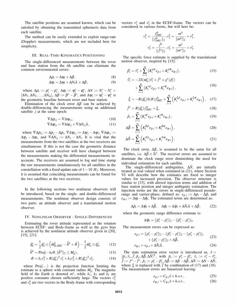
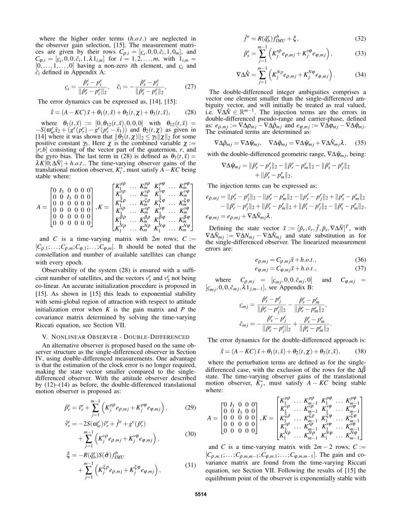
ities are depicted in Fig. 1, for single-difference, and Fig. 2for double-differenced.

Within 10 seconds the errors are smaller than 10cm. How-ever a small stationary error is present due to measurementnoise. The performance of the four observers are comparable,where the double-differenced observer has a better basestation estimate. The sinusoidal effect on the rover estimatesis caused by the chosen flight path. To showcase the expected

0 20 40 60 80 100 120-0.1

0

0.1

Err

or x

(m

)

0 20 40 60 80 100 120-0.1

0

0.1

Err

or y

(m

)

0 20 40 60 80 100 120

Time (s)

-0.1

0

0.1

Err

or z

(m

)

Fig. 1. Position errors of single-difference observer with real valued (red)and fixed ambiguities (blue). Base station error in dashed lines and rovererror in solid lines. The noise free simulation is shown with black dashedlines.

0 20 40 60 80 100 120-0.1

0

0.1

Err

or x

(m

)

0 20 40 60 80 100 120-0.1

0

0.1

Err

or y

(m

)

0 20 40 60 80 100 120

Time (s)

-0.1

0

0.1

Err

or z

(m

)

Fig. 2. Position errors of double-difference observer with real valued(magenta) and fixed ambiguities (yellow). Base station error in dashed linesand rover error in solid lines. The noise free simulation is shown with blackdashed lines.

effect a case without any noise is included in Fig. 1 and Fig.2 as black lines. It is evident that the observers with fixedintegers follow the sinusoidal effect best. No such effect ispresent during a straight flight path.

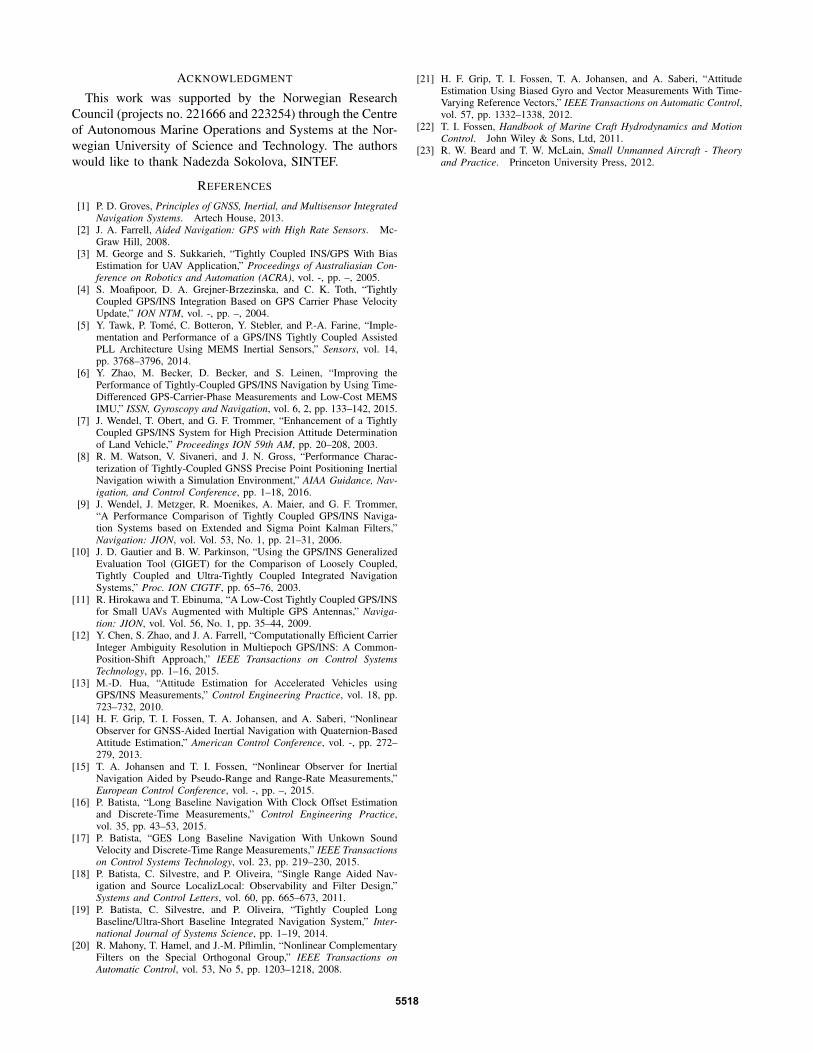
As an example of the real valued ambiguity errors, theestimation of ∆N11 and ∇∆N1,11 is depicted in Fig. 3. Similarbehavior is seen for the other satellites.

The ambiguities are fixed before 30s. The small differencebetween the four observer estimates is due to the real valuedambiguities being close to the true fixed value.

IX. CONCLUSIONS

Two nonlinear translational motion observers were pro-posed for estimating position, linear velocity and attitudeusing tightly coupled INS/GNSS integration in a dual GNSS-

5516

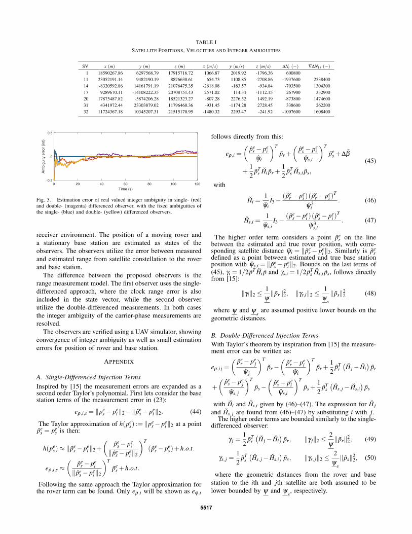
TABLE ISATELLITE POSITIONS, VELOCITIES AND INTEGER AMBIGUITIES

SV x (m) y (m) z (m) x (m/s) y (m/s) z (m/s) ∆Ni (−) ∇∆N1 j (−)1 18590267.86 6297568.79 17915716.72 1066.87 2019.92 -1796.36 600800 -

11 23052191.14 9482190.19 8876630.61 654.73 1108.85 -2708.86 -1937600 253840014 -8320592.86 14161791.19 21076475.35 -2618.08 -183.57 -934.84 -703500 130430017 9289670.11 -14108222.35 20708751.43 2571.02 114.34 -1112.15 267900 33290020 17875487.82 -5874206.28 18521323.27 -807.28 2276.52 1492.19 -873800 147460031 4341972.44 23303879.02 11796460.36 -931.45 -1174.28 2728.45 338600 26220032 11724367.18 10345207.31 21515170.95 -1480.32 2293.47 -241.92 -1007600 1608400

0 20 40 60 80 100 120

Time (s)

-0.5

0

0.5

Am

bigu

ity e

rror

(in

t)

Fig. 3. Estimation error of real valued integer ambiguity in single- (red)and double- (magenta) differenced observer, with the fixed ambiguities ofthe single- (blue) and double- (yellow) differenced observers.

receiver environment. The position of a moving rover anda stationary base station are estimated as states of theobservers. The observers utilize the error between measuredand estimated range from satellite constellation to the roverand base station.

The difference between the proposed observers is therange measurement model. The first observer uses the single-differenced approach, where the clock range error is alsoincluded in the state vector, while the second observerutilize the double-differenced measurements. In both casesthe integer ambiguity of the carrier-phase measurements areresolved.

The observers are verified using a UAV simulator, showingconvergence of integer ambiguity as well as small estimationerrors for position of rover and base station.

APPENDIX

A. Single-Differenced Injection TermsInspired by [15] the measurement errors are expanded as asecond order Taylor’s polynomial. First lets consider the basestation terms of the measurement error in (23):

eρ,i,s = ‖pes− pe

i ‖2−‖ pes− pe

i ‖2. (44)

The Taylor approximation of h(pes) := ‖pe

s− pei ‖2 at a point

pes = pe

s is then:

h(pes)≈ ‖ pe

s− pei ‖2 +

(pe

s− pei

‖ pes− pe

i ‖2

)T

(pes− pe

s)+h.o.t.

eρ,i,s ≈(

pes− pe

i‖ pe

s− pei ‖2

)T

pes +h.o.t.

Following the same approach the Taylor approximation forthe rover term can be found. Only eρ,i will be shown as eϕ,i

follows directly from this:

eρ,i =

(pe

r− pei

ψi

)T

pr +

(pe

s− pei

ψs,i

)T

pes +∆β

+12

pTr Hi pr +

12

pTs Hs,i ps,

(45)

with

Hi =1ψi

I3−(pe

r− pei )(pe

r− pei )

T

ψ3i

. (46)

Hs,i =1

ψs,iI3−

(pes− pe

i )(pes− pe

i )T

ψ3s,i

. (47)

The higher order term considers a point per on the line

between the estimated and true rover position, with corre-sponding satellite distance ψi = ‖pe

r − pei ‖2. Similarly is pe

sdefined as a point between estimated and true base stationposition with ψs,i = ‖pe

s− pei ‖2. Bounds on the last terms of

(45), γi = 1/2 pT Hi p and γs,i = 1/2pTs Hs,i ps, follows directly

from [15]:

‖γi‖2 ≤1ψ‖ pr‖2

2, ‖γs,i‖2 ≤1

ψs

‖ ps‖22 (48)

where ψ and ψs

are assumed positive lower bounds on thegeometric distances.

B. Double-Differenced Injection TermsWith Taylor’s theorem by inspiration from [15] the measure-ment error can be written as:

eρ,i j =

( per− pe

j

ψ j

)T

pr−(

per− pe

iψi

)T

pr +12

pTr(H j− Hi

)pr

+

( pes− pe

j

ψs, j

)T

ps−(

pes− pe

iψs,i

)T

ps +12

pTs(Hs, j− Hs,i

)ps

with Hi and Hs,i given by (46)–(47). The expression for H jand Hs, j are found from (46)–(47) by substituting i with j.

The higher order terms are bounded similarly to the single-differenced observer:

γ j =12

pTr(H j− Hi

)pr, ‖γ j‖2 ≤

2ψ‖ pr‖2

2, (49)

γs, j =12

pTs(Hs, j− Hs,i

)ps, ‖γs, j‖2 ≤

2ψ

s

‖ps‖22, (50)

where the geometric distances from the rover and basestation to the ith and jth satellite are both assumed to belower bounded by ψ and ψ

s, respectively.

5517

ACKNOWLEDGMENT

This work was supported by the Norwegian ResearchCouncil (projects no. 221666 and 223254) through the Centreof Autonomous Marine Operations and Systems at the Nor-wegian University of Science and Technology. The authorswould like to thank Nadezda Sokolova, SINTEF.

REFERENCES

[1] P. D. Groves, Principles of GNSS, Inertial, and Multisensor IntegratedNavigation Systems. Artech House, 2013.

[2] J. A. Farrell, Aided Navigation: GPS with High Rate Sensors. Mc-Graw Hill, 2008.

[3] M. George and S. Sukkarieh, “Tightly Coupled INS/GPS With BiasEstimation for UAV Application,” Proceedings of Australiasian Con-ference on Robotics and Automation (ACRA), vol. -, pp. –, 2005.

[4] S. Moafipoor, D. A. Grejner-Brzezinska, and C. K. Toth, “TightlyCoupled GPS/INS Integration Based on GPS Carrier Phase VelocityUpdate,” ION NTM, vol. -, pp. –, 2004.

[5] Y. Tawk, P. Tomé, C. Botteron, Y. Stebler, and P.-A. Farine, “Imple-mentation and Performance of a GPS/INS Tightly Coupled AssistedPLL Architecture Using MEMS Inertial Sensors,” Sensors, vol. 14,pp. 3768–3796, 2014.

[6] Y. Zhao, M. Becker, D. Becker, and S. Leinen, “Improving thePerformance of Tightly-Coupled GPS/INS Navigation by Using Time-Differenced GPS-Carrier-Phase Measurements and Low-Cost MEMSIMU,” ISSN, Gyroscopy and Navigation, vol. 6, 2, pp. 133–142, 2015.

[7] J. Wendel, T. Obert, and G. F. Trommer, “Enhancement of a TightlyCoupled GPS/INS System for High Precision Attitude Determinationof Land Vehicle,” Proceedings ION 59th AM, pp. 20–208, 2003.

[8] R. M. Watson, V. Sivaneri, and J. N. Gross, “Performance Charac-terization of Tightly-Coupled GNSS Precise Point Positioning InertialNavigation wiwith a Simulation Environment,” AIAA Guidance, Nav-igation, and Control Conference, pp. 1–18, 2016.

[9] J. Wendel, J. Metzger, R. Moenikes, A. Maier, and G. F. Trommer,“A Performance Comparison of Tightly Coupled GPS/INS Naviga-tion Systems based on Extended and Sigma Point Kalman Filters,”Navigation: JION, vol. Vol. 53, No. 1, pp. 21–31, 2006.

[10] J. D. Gautier and B. W. Parkinson, “Using the GPS/INS GeneralizedEvaluation Tool (GIGET) for the Comparison of Loosely Coupled,Tightly Coupled and Ultra-Tightly Coupled Integrated NavigationSystems,” Proc. ION CIGTF, pp. 65–76, 2003.

[11] R. Hirokawa and T. Ebinuma, “A Low-Cost Tightly Coupled GPS/INSfor Small UAVs Augmented with Multiple GPS Antennas,” Naviga-tion: JION, vol. Vol. 56, No. 1, pp. 35–44, 2009.

[12] Y. Chen, S. Zhao, and J. A. Farrell, “Computationally Efficient CarrierInteger Ambiguity Resolution in Multiepoch GPS/INS: A Common-Position-Shift Approach,” IEEE Transactions on Control SystemsTechnology, pp. 1–16, 2015.

[13] M.-D. Hua, “Attitude Estimation for Accelerated Vehicles usingGPS/INS Measurements,” Control Engineering Practice, vol. 18, pp.723–732, 2010.

[14] H. F. Grip, T. I. Fossen, T. A. Johansen, and A. Saberi, “NonlinearObserver for GNSS-Aided Inertial Navigation with Quaternion-BasedAttitude Estimation,” American Control Conference, vol. -, pp. 272–279, 2013.

[15] T. A. Johansen and T. I. Fossen, “Nonlinear Observer for InertialNavigation Aided by Pseudo-Range and Range-Rate Measurements,”European Control Conference, vol. -, pp. –, 2015.

[16] P. Batista, “Long Baseline Navigation With Clock Offset Estimationand Discrete-Time Measurements,” Control Engineering Practice,vol. 35, pp. 43–53, 2015.

[17] P. Batista, “GES Long Baseline Navigation With Unkown SoundVelocity and Discrete-Time Range Measurements,” IEEE Transactionson Control Systems Technology, vol. 23, pp. 219–230, 2015.

[18] P. Batista, C. Silvestre, and P. Oliveira, “Single Range Aided Nav-igation and Source LocalizLocal: Observability and Filter Design,”Systems and Control Letters, vol. 60, pp. 665–673, 2011.

[19] P. Batista, C. Silvestre, and P. Oliveira, “Tightly Coupled LongBaseline/Ultra-Short Baseline Integrated Navigation System,” Inter-national Journal of Systems Science, pp. 1–19, 2014.

[20] R. Mahony, T. Hamel, and J.-M. Pflimlin, “Nonlinear ComplementaryFilters on the Special Orthogonal Group,” IEEE Transactions onAutomatic Control, vol. 53, No 5, pp. 1203–1218, 2008.

[21] H. F. Grip, T. I. Fossen, T. A. Johansen, and A. Saberi, “AttitudeEstimation Using Biased Gyro and Vector Measurements With Time-Varying Reference Vectors,” IEEE Transactions on Automatic Control,vol. 57, pp. 1332–1338, 2012.

[22] T. I. Fossen, Handbook of Marine Craft Hydrodynamics and MotionControl. John Wiley & Sons, Ltd, 2011.

[23] R. W. Beard and T. W. McLain, Small Unmanned Aircraft - Theoryand Practice. Princeton University Press, 2012.

5518