Embed Size (px)
Citation preview

Tilburg University
Econometric models of child mortality dynamics in rural Bangladesh
Saha, U.R.
Publication date:2012
Link to publication
Citation for published version (APA):Saha, U. R. (2012). Econometric models of child mortality dynamics in rural Bangladesh. Tilburg: CentER,Center for Economic Research.
General rightsCopyright and moral rights for the publications made accessible in the public portal are retained by the authors and/or other copyright ownersand it is a condition of accessing publications that users recognise and abide by the legal requirements associated with these rights.
- Users may download and print one copy of any publication from the public portal for the purpose of private study or research - You may not further distribute the material or use it for any profit-making activity or commercial gain - You may freely distribute the URL identifying the publication in the public portal
Take down policyIf you believe that this document breaches copyright, please contact us providing details, and we will remove access to the work immediatelyand investigate your claim.
Download date: 23. Jul. 2019

Econometric Models of Child Mortality
Dynamics in Rural Bangladesh
Unnati Rani Saha


Econometric Models of Child Mortality
Dynamics in Rural Bangladesh
Proefschrift
ter verkrijging van de graad van doctor aan Tilburg University op gezag van de rector magnificus,
prof. dr. Ph. Eijlander, in het openbaar te verdedigen ten overstaan van een door het college voor
promoties aangewezen commissie in de aula van de Universiteit op
vrijdag 10 februari 2012 om 12.15 uur door
Unnati Rani Saha
Geboren op 15 maart 1966 te Narayanganj, Bangladesh

Promotor:
prof. dr. A.H.O. van Soest
Commissieleden:
prof. dr. F.M.P. Vermeulen
dr. G.E. Bijwaard
dr. K.G. Carman
dr. S. Padmadas

Acknowledgements
Working as a Ph.D. student in Tilburg University was a magnificent as well as a
challenging experience for me. In all these years, many people were directly and indirectly
instrumental in shaping my academic career. It was hardly possible for me to thrive in my
doctoral work without the precious support of all these people. Here is a small tribute to those
people behind the screen who helped me to make my dream come true.
First of all, I wish to thank my respected supervisor Arthur van Soest for introducing me to the
world of econometric modeling and its application on demographic research. Here, I would like
to refer to the article of Bhalotra and Van Soest (2006), which I read in 2006 and was my key
impetus to learn econometric models. After long email discussions during February-March 2007
Arthur invited me as a visiting researcher in Tilburg University. During that period, I shared my
research ideas with Arthur and developed a concept note, and presented my research findings in
the Department of Econometrics and Operations Research. I then also applied for a Ph.D.
position in the CentER Graduate School.
I got accepted and joined the CentER Graduate School in September 2007. Since then Arthur
taught me and guided me continuously for four years in order to accomplish my goal of writing a
dissertation. It was only due to his valuable guidance, cheerful enthusiasm and ever-friendly
nature that I was able to complete my research work facing so many constraints. He has
enlightened me through his wide knowledge of econometric modeling technique and his deep
intuitions about where it should go and what is necessary to get there, and to make consistency of
references and text. I am ever grateful to him.
I wish to express my gratitude to Dr. Govert E. Bijwaard, senior researcher of the Netherlands
Interdisciplinary Demographic Institute (NIDI) for his open mind to deliberately transferring his
programming skill duration analysis and valuable suggestions. The fifth chapter of my thesis is
co-authored with him.
I have greatly enjoyed these days in Tilburg and gained a lot of experience on econometric
modeling technique, writing and publishing in high dimensional scientific journals. I strongly
believe that “to become successful, one has to have will and skill–but the will must be stronger
than the skill” as opined by Paulo Chilo. My “will” helped me to make more contacts and
achieve success in my life.
“Look at the sky. We are not alone. The whole universe is friendly
to us and conspires only to give the best to those who dream and
work” A.P.J. Abdul Kalam, ex-president of India
I got my mental strength through reading the above quote. The society from where I come is
highly patriarchal, almost non-cooperative for female higher education. The essence of the above
quote inspired me to hold my head high against all odds. A big thank you to my husband Uttam
Kumar Saha who allowed me to get higher education.
I wish to thank the people of the Human Resources office, the secretariat of the Department of
Econometrics & Operations Research and CentER Graduate Office of Tilburg University for all
administrative help. From the bottom of my heart I wish to thank Korine Bor who was always
willing to help me.
I deeply appreciate Dr. Peter Kim Streatfield, head of Demographic and Health Surveillance
Systems (HDSS), Matlab, International Centre for Diarrhoel Disease Research, Bangladesh
(ICDDR,B) for providing the data for my Ph.D. research. I am grateful to Dr. Carel van Mels
for his kind recommendation to get permission for using HDSS data in my dissertation. I am
grateful to all donors who continuously support ICDDR,B.

v
I am obliged to Dr. Charles P. Larson, former head of the Health Systems and Infectious
Diseases (HSID) Division, ICDDR,B for recommending me for availing study leave to
accomplish my dissertation at Tilburg University. I deeply express my gratitude to the staff of
Human Resources, Training & Development of ICDDR,B for all administrative help. Finally, I
greatly express my gratitude to Dr. Alejandro Cravioto, executive director of ICDDR,B for
granting me study leave from November, 2007 till date.
In my personal note I wish to thank Dr. Radheshyam Bairagi, former senior scientist, ICDDR,B
and Dr. Abbas Uddin Bhuyia, deputy executive director, ICDDR,B who always inspired me with
their mails.
I am grateful to all: mentors, teachers, friends, colleagues, family members, relatives and well
wishers and to none other than the Almighty.
I wish to thank my mother Suruchi Bala Saha who always encourages me to achieve more and
more education. I dip my head with respect to my father Nirmal Chandra Saha’s eternal soul
whom I have lost in 1994. I acknowledge my daughters Uditi’s and Rittika’s patience,
understanding and acceptance for their mom’s education for which they had to compromise a lot
in their life.
I bow my head in gratitude for all those who inspired me in accomplishing this impossible job.

vi
Contents
Acknowledgements
1 Introduction 1
1.1 Background ……………………………………………………………………………….1
1.2 The Matlab Area ………………………………………………………………………….2
1.3 Health Systems in Matlab, Bangladesh …………………………………………………..3
1.4 Methodological issues and data …………………………………………………………..3
1.5 Research issues …………………………………………………………………………...4
Annex ……………………………………………………………………………………..6
2 Infant Death Clustering in Families 8
2.1 Introduction ……………………………………………………………………………...8
2.2 Background ……………………………………………………………………………...9
2.3 Data …………………………………………………………………………………….11
2.3.1 Health and Demographic Surveillance System, Matlab …………………………11
2.3.2 Study sample …………………………………………………………………….12
2.3.3 Variables and descriptive statistics ……………………………………………...12
2.4 Model specification ……………………………………………………………………14
2.5 Estimation results ………………………………………………………………………16
2.6 Alternative specifications and robustness checks ……………………………………...18
2.7 Discussion and conclusion ……………………………………………………………..19
Tables …………………………………………………………………………………..22
Graphs ………………………………………………………………………………….26
Annex …………………………………………………………………………………..27
3 Childhood Mortality and Reproductive Behaviour: Causal Analysis 29
3.1 Introduction ………………………………………………………………………….29
3.2 Overview of causal mechanisms …………………………………………………….30
3.3 Literature review …………………………………………………………………….32
3.4 Policy implications …………………………………………………………………..33
3.5 Data ………………………………………………………………………………….33
3.5.1 Study sample …………………………………………………………………33
3.5.2 Variables and descriptive statistics …………………………………………..34
3.6 Model specification ………………………………………………………………….35
3.7 Estimation results ……………………………………………………………………39
3.8 Simulations ………………………………………………………………………….42
3.9 Discussion and Conclusion ………………………………………………………….45
Tables ………………………………………………………………………………..48
Graphs ……………………………………………………………………………….53
4 Family Planning Practice and Infant Mortality 55
4.1 Introduction …………………………………………………………………………..55
4.2 Data …………………………………………………………………………………...57
4.2.1 ICDDR,B area and interventions ……………………………………………….57
4.2.2 Study sample ……………………………………………………………………58
4.2.3 Variables and descriptive statistics ……………………………………………..58
4.3 Model …………………………………………………………………………………60
4.4 Estimation results ……………………………………………………………………..64
4.5 Simulations …………………………………………………………………………...67
4.6 Alternative model specifications ……………………………………………………...69
4.7 Discussion and conclusion ……………………………………………………………70
Tables …………………………………………………………………………………73
Graphs ………………………………………………………………………………...76
Annex …………………………………………………………………………………77

vii
5 Cause-specific Neonatal Deaths 78
5.1 Introduction ……………………………………………………………………………. 78
5.2 Background ……………………………………………………………………………..79
5.3 Data ……………………………………………………………………………………..81
5.3.1 Causes of death …………………………………………………………………...81
5.3.2 Socio-demographic variables ……………………………………………………..82
5.3.3 Distribution of causes of deaths …………………………………………………..82
5.3.4 Cumulative incidence of cause-specific death …………………………................83
5.4 Modeling ………………………………………………………………………………..83
5.5 Estimation results ……………………………………………………………………….85
5.5.1 Communicable versus Non-communicable diseases: Covariate effects ………….85
5.5.2 CDs and NCDs: Unobserved heterogeneity……………………………………….87
5.5.3 Model with four causes of death: Covariate effects ………………………………87
5.5.4 Model with four causes of death: Unobserved heterogeneity …………………….89
5.5.5 Cumulative incidences functions …………………………………………………89
5.6 Discussion and conclusion……………………………………………………………....90
Tables …………………………………………………………………………………...94
Graphs …………………………………………………………………………............100
Annex ………………………………………………………………………………….103
6 Summary and conclusion …………………………………………………………………104
Bibliography …..........................................................................................................................106

Chapter 1
Introduction
Health transition is an important aspect of demographic change and a complex process
comprising demographic, epidemiological and health care transitions. It is manifested in rising
life expectancy at birth due to changes in the fertility, mortality and morbidity profile of a
population. Demographic transition brings down birth and death rates and changes the age
structure; epidemiological transition reflects changes in the causes of death, from infectious
(pandemic) diseases to non-communicable (degenerative, human-made) diseases (Caldwell et al.
1990; Omran 1982). However, the causal mechanisms of demographic changes are unclear. The
focus of my thesis is to uncover these causal mechanisms, and to quantify the epidemiological
shifts over time, taking into account phenomena that hamper a straightforward empirical analysis,
such as competing risks, observed and unobserved confounding factors, and reverse causality.
This analysis may influence policy development in countries such as Bangladesh, whose ability
to meet Millennium Development Goal 4 (see United Nations 2001) is currently in doubt.
1.1 Background
According to demographic transition theory, there is a strong correlation between childhood
mortality and fertility. Empirical evidence has shown that a decline in childhood mortality is
often a prerequisite for fertility decline (Chowdhury et al. 1976; Matthiesson and McCann 1978;
Pritchett 1994; Wolpin 1997). Other studies have emphasized the reverse direction of this
causation, e.g., high fertility and the close birth-spacing associated with it cause an increase in
child mortality (Cleland and Sathar 1984; Curtis et al. 1993). Yet another set of studies
emphasized that the analysis of the direction of causality with birth interval data is hampered by
the close interrelations between child mortality and fertility (Zimmer 1979; Santow and Bracher
1984).
Family planning is also related to health transition in multifaceted ways. Through family
planning practice, a couple can decide the time of birth, the time span between two births, and
the (maximum) number of children they want to have. Thus, once family size declines, there is
an added incentive to ensure the survival of children. In the developing world, some success is
evident in reducing child death in small families (see for example, Caldwell and Caldwell 1978).
Family planning practice can also avoid births at extreme age and at short intervals, which have
detrimental effects on child mortality. Yet another set of arguments posit that if the society is not

2
overly concerned with the sexual purity of its women, it is more likely to permit girls to go to
school and even to stay there when they reach puberty, which in turn will inevitably transfer
more family resources towards children and ultimately towards wives (Caldwell 1993).
There is a large literature on the determinants of childhood mortality in developing
countries, focusing on, for example, the fact that children of very young mothers or mothers with
little or no schooling are at higher risk. Moreover, demographic data from many countries have
revealed that child deaths are clustered within families. See, for example, Das Gupta (1990) for
India, Gubhaju (1985) for Nepal, Guo and Rodriguez (1992) and Guo (1993) for Guatemala,
Curtis et al. (1993) and Sastry (1997) for Brazil, or Madise and Diamond (1995) for Malawi. It is
argued by demographers that this small fraction of deaths may be a product of infectious disease
or biological differences, but probably most of the explanation lies in different levels of family
care or interaction with the health system.
However, with the available explanation and the evidence of correlated sibling death, the
causal relationship of child deaths and fertility, and epidemiological transition, the empirical
literature is indeed limited on areas such as the causal mechanisms in the relationship between
fertility and mortality, or how to accommodate the correlation with sibling death at an aggregate
level or at the level of causes of death (see for example, DaVanzo et al. 2008; Yeakey et al. 2009;
Bhatia 1989). These particular issues form the focus of four separate papers included in my
thesis.
1.2 The Matlab Area
Matlab Thana is an administrative region in the Chandpur district of Bangladesh. Matlab is
located about 55 km southeast of Dhaka, the capital city of Bangladesh. The climate is sub-
tropical with three seasons: monsoon, cool-dry and hot-dry. The average annual rainfall of 2159
mm is concentrated in the monsoon season extending from June to September. Being flat and
low-lying it is subject to annual flooding by many canals and rivers which cross the area. The
population density is about 1,100 per km2
residing in 142 villages. The area is a typical rural
river delta area of Bangladesh. Almost 90% of the population are Muslims and the great majority
of the remainder are Hindus; all of them speak Bangla. The principle economic activities are
agriculture and fishing. For most dwellings, roof material is tin (95%), while in 30% tin was used
for wall material. Travel within Matlab Thana and between the villages is mostly by foot or
rickshaw or country boat, particularly during the monsoon season.
Since 1963, the ICDDR,B Centre for Health and Population Research, formally Cholera
Research Laboratory, has been implementing a health related research programme. The health
and Demographic Surveillance System (HDSS), formally Demographic Surveillance System
(DSS), is one of the major components of this field programme. Since 1966, the HDSS has been
maintaining the registration of births, deaths, and migration, in addition to carrying out periodical
censuses in 149 villages 70 in ICDDR,B area and 79 in the comparison area (so called
Chapter 1: Introduction
3
government area). Due to river erosion, 7 villages disappeared from the comparison area in 1987,
leaving 142 villages in the HDSS. In 2000, 3 of the 70 villages of ICDDR,B area were
transferred to the comparison area. A map is given in the Annex.
1.3 Health Systems in Matlab, Bangladesh
In 1977, the International Centre for Diarrhoeal Disease Research, Bangladesh (ICDDR,B)
started to provide extensive maternal-child health and family planning (MCH/FP) services, in
addition to existing government health services, in half (70 villages) of the Health and
Demographic Surveillance System (HDSS) area, called the ICDDR,B area. The other half (79
villages), the comparison area, continued to receive only the standard government health services.
The MCH/FP project includes provision of domiciliary family planning services, simple nutrition
education, tetanus toxoid immunization for pregnant women (which was modified in 1981 to
include all women of reproductive age), community-based oral rehydration therapy, and measles
immunization. These services were introduced incrementally phase by phase (see Annex, Table
1). In the ICDDR,B area, there are several ICDDR,B sub-centres providing treatment for minor
illnesses and basic emergency obstetric care (EOC), and a permanent hospital that provides
treatment for diarrhoeal diseases. In order to understand the way in which better health services
shape child health, I analyze the data from the area with the better health care services in addition
to the government health services (ICDDR,B area), as well as the data from an area with
standard government health services only (the comparison area - a typical rural area of
Bangladesh).
1.4 Methodological issues and data
The primary focus of my dissertation is to apply an econometric approach to empirical research
on child mortality dynamics in Bangladesh. In econometrics, the assumptions of the underlying
population model are couched in terms of correlations, conditional expectations, and conditional
variances-covariances, or conditional distributions, can usually be given behavioral content. In
demographic research, the application of econometrics can bring greater insight into the
behavioral context than can mere quantitative measures. Several researchers, such as Bongaarts
(1987) or DaVanzo et al. (2008), saw the importance of investigating and disentangling the
various causal and non-causal relationships between birth-spacing, fertility decisions and
childhood mortality, in countries in demographic transition such as Bangladesh.
In social sciences research, we very often fail to include potential observed covariates in
the model, which might lead to an unobserved heterogeneity (unobserved variability) in the
response variable. This is a common phenomenon for cross section or panel data: observations
for the same unit are influenced by the same (shared) unit-specific time invariant unobserved
heterogeneity. Thus, while the major concern of statistical modeling is to explain the variability
in the response variable in terms of the effects of observed covariates, called ‘observed
heterogeneity’, failing to be able to include all relevant covariates due to data limitations leads to
4
unobserved heterogeneity. This needs to be accounted for in the analyses to obtain unbiased
estimates.
Causal analysis (investigating cause and effect) is an important aspect of econometrics.
Utilizing this concept in demographic research, part of my thesis investigates the bi-causal
relationship between fertility and mortality, and for example, how birth spacing shapes this
relationship. I also use the concept of state dependence as used in the labor economics literature
on unemployment to investigate for example, the clustering of deaths of siblings. Since
decisions are inherently dynamic and sequential, the static models often employed to study
variables such as mortality and fertility can produce misleading estimates (Wolpin 1997;
Rosenzweig and Wolpin 1988). The main motivation for this thesis is to follow the modelling
framework of Arulampalam and Bhalotra (2006) and Bhalotra and van Soest (2008) in order to
account for the dynamics and the simultaneous nature of mortality-birth spacing and fertility
sequencing decisions, and for endowments (persistent mother-specific traits), modeled as
unobserved heterogeneity components within families. A recent study on investigating the causal
impact of fertility timing on education also noted the importance of such dynamic models when
decisions are sequential (see Stange 2011).
All four papers on which the chapters are based, aim to analyze information on
individuals (child level information) and families (mother level information) over the period
1982-2005. In the second and third chapters, information on the complete pregnancy history of a
mother is used, for example, live births, deaths and several indicators of socioeconomic status,
are recorded for the population of about 220,000 people in the Matlab Health and Demographic
Surveillance System (HDSS) area, split into ICDDR,B and comparison area. In the fourth
chapter, the modelling framework used in the third chapter is extended by including the mother’s
contraceptive use status after each birth. The fifth chapter uses the birth history of each mother
and their live births, neonatal deaths and socio economic indicators. In this chapter, data obtained
on both complete and incomplete birth histories are used, because birth spacing is not the
primary interest of analysis. Although, it remains important to include birth spacing in the list of
explanatory variables, it is avoided because of endogeneity problems making the modeling more
complicated. It remains a topic for further research.
1.5 Research issues
The research theme of my dissertation is common and has long been of interest to demographers.
Apart from previous research on this issue, using several advanced econometric techniques to
answer the related research questions in all chapters, I have worked jointly with co-authors and
developed four separate but related papers. All chapters of my dissertation are based on papers
except the introduction in the first chapter, and the overall summary and conclusion in the last
chapter. In the second chapter, we investigate sibling death clustering in families and use of
better health services. We use an existing modeling framework distinguishing two explanations
for death clustering: (observed and unobserved) heterogeneity across families, and a causal
“scarring” effect of infant mortality of one child on the survival chances of the next child.

Chapter 1: Introduction
5
In the third chapter, to distinguish causal mechanisms from unobserved heterogeneity and
reverse causality, we used dynamic panel data techniques, building on recent work by Bhalotra
and van Soest (2008). This model incorporates various causal mechanisms as well as unobserved
heterogeneity, exploiting the sequence of all births and deaths to a mother to accommodate the
correlations between the mortality risks of consecutive children and birth intervals. We compare
the results in a treatment area (the ICDDR,B area) with extensive health services and a
comparison area with the standard health services provided by the government.
In the fourth chapter, we analyze the effect of family planning on child survival, which
remains an important issue but is not straightforward, because of several mechanisms linking
family planning, birth intervals, total fertility, and child survival. This study uses a dynamic
model jointly explaining infant mortality, whether contraceptives are used after each birth, and
birth intervals. Infant mortality is determined by the preceding birth interval and other covariates
(such as socio-economic status). Decisions about using contraceptives after each birth are driven
by similar covariates, survival status of the previous child, and the family’s gender composition.
Birth spacing is driven by contraceptive use and other factors.
In the fifth chapter, we focus on explaining cause-specific neonatal mortality and employ
a competing risks model, incorporating both observed and unobserved heterogeneity and
allowing the heterogeneity terms for the various causes to be correlated. We employ a
proportional hazard model with a piecewise constant baseline hazard.

6
Annex
Source: HDSS, Matlab, volume 35; Registration of health and demographic events 2002;
Scientific report number 91.
Note: Government area is referred as comparison area in this thesis.

Chapter 1: Introduction
7
Note: The Table is copied from LeGrand and Phillips 1996.
Chapter 2
Infant death clustering in families: magnitude,
causes, and the influence of better health services,
Bangladesh 1982–20051
2.1 Introduction
We report on an analysis of infant mortality in Bangladesh that focused on explaining the
phenomenon of death clustering within families. The study used dynamic panel-data models that
distinguished between two explanations of death clustering: (observed and unobserved)
heterogeneity across families, and state dependence - a causal 'scarring' effect of the death of one
infant on the survival chances on the next born child. Arulampalam and Bhalotra (2006, 2008)
applied the logit version of this model to Indian data, while Omariba et al. (2008) used a similar
probit model to analyse infant mortality in Kenya. Our study was the first to apply this type of
model to Bangladesh.
Child mortality in Bangladesh remains an important issue. Under-five mortality declined
sharply during the last decades of the previous century, but the reduction is levelling off and
child mortality is not declining fast enough to meet Millennium Development Goal 4 of reducing
under-five mortality by two-thirds between 1990 and 2015 (see United Nations 2001). Thus
further reduction of child mortality remains a significant challenge. As in most developing
countries, infant deaths (deaths before the age of twelve months) form the largest part of under-
five mortality and therefore deserve special attention. Moreover, as for many other countries,
data for Bangladesh reveal clear evidence of infant death clustering: the proportion of children
who die in infancy is much larger among children whose previous sibling also died in infancy
than among children whose sibling survived; see, for example, Swenson (1978), Koenig et al.
1 This chapter is joint work with Arthur van Soest, Tilburg University and published as Saha and van Soest (2011).
This paper has been presented in the Health & Labour Group seminar, Tilburg University, International Union for
the Scientific Study of Population (IUSSP) 2009, Marrakesh, Morocco, and published in the Journal of Population
Studies, November, 2011. We thank seminar participants, three anonymous referees and chief editor of Population
Studies Journal for helpful suggestions and insightful comments.

Chapter 2: Sibling death clustering
9
(1990), Zenger (1993), Majumder et al. (1997), or Alam and David (1998). Understanding the
causes of infant death clustering may give insight into how multiple deaths in a family could be
prevented, and may thus contribute to the goal of reducing infant and child mortality.
Our study was based on prospective panel-data from 1982 to 2005 on mothers and
children from the Matlab region, a rural area located 60 km southeast of Dhaka. Two sets of
villages were covered: an intervention area with non-standard health services, and a (control)
area with standard government-provided health care facilities. We expected the differences
between the two areas to reveal the effects of additional health care services on infant mortality
and death clustering.
2.2 Background
The large literature on the determinants of infant mortality in developing countries includes
reports of studies from many countries showing that child deaths are clustered within families.
See, for example, Das Gupta (1990) for India, Gubhaju (1985) for Nepal, Guo and Rodriguez
(1992) and Guo (1993) for Guatemala, Curtis et al. (1993) and Sastry (1997) for Brazil, or
Madise and Diamond (1995) for Malawi. Explanations of this phenomenon of death clustering
are discussed extensively in, for example, Omariba et al. (2008, Section 2), and we summarize
them only briefly here.
First, the clustering may be due to observed and unobserved characteristics of the mother,
the family, or the local community; examples are adverse genetic traits, maternal health
problems, inability to take care of the child, or environmental factors such as unsafe water supply
or limited access to health care. All these factors may increase the risk for all children in a given
family. It is also evident that death clustering is more pronounced among women of higher parity
(Zaba and David 1996).
Second, death-clustering may be due to a causal effect of the death of one child on the
survival chances of later siblings, an effect described as '(positive) scarring' (Arulampalam and
Bhalotra 2006). One possible mechanism is that a child’s death leaves the mother depressed and
that this affects the next child’s health in the womb or in infancy (on the 'depression hypothesis',
see Steer et al. 1992 or Rahman et al. 2004). Another possible positive scarring mechanism is the
'replacement hypothesis': women whose child dies have their next birth sooner than they would
have done otherwise, resulting in closely-spaced pregnancies that may lead to the health of the
next born child being affected by nutritional depletion (see, e.g., Hobcraft et al. 1983). There
might also be 'negative scarring' mechanisms': a reduced risk of infant death following the death
of a sibling's death in infancy, owing to learning effects or to reduced competition for family
resources (Alam 1995).
The older studies often attribute death clustering to socio-demographic covariates: either
a causal scarring effect (the previous sibling’s survival status being included as a covariate), or
unobserved family-level or community-level heterogeneity (with family-specific or community-
10
specific effects). A good example is Zenger (1993), who estimates models with either scarring
or unobserved heterogeneity, but not both. Some studies include both unobserved heterogeneity
and scarring (Guo 1993; Curtis et al. 1993; Sastry 1997; Bolstad and Manda 2001), but without
accounting for the (bias induced by) potential correlation between the unobserved heterogeneity
term and the previous child’s survival-status dummy.
A major innovation was the study by Arulampalam and Bhalotra (2006), which explains
infant mortality with an econometric dynamic panel-data model that at the same time also
captures unobserved heterogeneity and the causal positive or negative scarring mechanisms (also
referred to as 'state dependence' if panel data are used). Their model accounts for the endogeneity
of previous sibling-survival status, thus avoiding the potential bias in previous studies.
Arulampalam and Bhalotra (2006, 2008) applied this model to data for India and Omariba et al.
(2008) used a similar model for Kenya. These studies all find positive scarring effects of varying
sizes. For example, Arulampalam and Bhalotra (2008, Table 2) present separate estimates for 15
Indian states and find that, keeping other factors constant, infant death of the previous sibling
increases the likelihood of infant death by between 2.2 percentage points (West Bengal and
Punjab; two of the richest states) and 9.2 percentage points (Haryana). For Kenya, Omariba et al.
(2008, p. 324) find a scarring effect of 4.8 percentage points. Since these estimates do not control
for the length of the preceding birth interval, the estimated scarring effects include the effect
through the birth interval (death of a child speeds up birth of the next child, and a shorter birth
interval increases mortality risk). Arulampalam and Bhalotra (2008, Table 4) also present
estimates with the preceding birth interval kept constant, which are estimates of the effects of
scarring mechanisms that do not work through the birth interval. These estimates are still
positive and in most cases significant, but 30 to 50 per cent smaller than the scarring effect, not
controlling for preceding birth interval length. Bhalotra and van Soest (2008) extended this
model by allowing birth intervals and fertility decisions to be endogenous to mortality. Keeping
birth intervals constant, they find a scarring effect on neonatal mortality (death in the first month
after birth) of 4.16 percentage points (p. 282).
The existing literature on child mortality includes a number of papers that focus on
Bangladesh. A paper by Hale et al. (2006) used the same source of data that we used. They find
that about 20 per cent of the differences in infant and child mortality between the intervention
area and the comparison area can be explained by differences in reproductive behaviour (birth
intervals, parity), and attribute the remaining part to differences in the quality of health services.
In another paper, DaVanzo et al. (2007) analyse not only infant and child mortality but also
stillbirths, miscarriages, and induced abortion. They conclude that mothers with a preceding non-
live birth should receive counselling and monitoring. DaVanzo et al. (2008) find that shorter
birth intervals are followed by higher mortality and conclude that some of their results are
consistent with nutritional depletion of the mother and others with sibling competition. They also
find support for mother-specific unobserved heterogeneity. They recommend that future research
should use models that can disentangle these mechanisms. None of the preceding studies on
Bangladesh use the dynamic panel-data models of Arulampalam and Bhalotra (2006, 2008) or

Chapter 2: Sibling death clustering
11
Omariba et al. (2008) to account properly for the various explanations of death clustering. Our
study was directed at doing so.
Previous studies that used dynamic panel-data models are based on Demographic Health
Surveys (DHS), for either India or Kenya. The samples were cross-sections of mothers who
retrospectively reported their complete birth histories. Rich background information on, for
example, the family’s socio-economic status or the facilities in the area of residence was
available, but only at the time of the survey. If these variables were used to explain infant
mortality, the variables measured at the time of the survey were used as proxies for the same
(unobserved) variables at the time of childbirth, which is why the existing studies used only
background variables that were less likely to change over time. Our data were different: data
were collected prospectively, avoiding possible recall error in birth and death histories and
survival bias caused by mothers’ mortality (Rosenblum 2009). Several variables were measured
around the time of childbirth (like the father’s occupational status and access to piped water; see
also Section 3). Moreover, we knew whether women moved and could therefore select a sample
of individuals who lived permanently in the same geographic area.
2.3 Data
2.3.1 Health and Demographic Surveillance System, Matlab
Since 1966, the International Centre for Diarrhoeal Disease Research, Bangladesh (ICDDR,B)
has maintained a Health and Demographic Surveillance System (HDSS) in Matlab, a rural area
located 60 km southeast of Dhaka. All the following data are recorded in this area for the
complete population of about 220,000 people: births, deaths, causes of death, pregnancy histories,
migration in and out of the area, marriages, divorces, and several indicators of socioeconomic
status. The same data source has been used in many other studies of child mortality in
Bangladesh, such as the studies of Bairagi et al. (1999), Majumder et al. (1997), Hale et al.
(2006), Razzaque et al. (2007), and DaVanzo et al. (2007, 2008).
The ICDDR,B started the Maternal Child Health and Family Planning Programme
(MCH-FP) project in October 1977 in half of the HDSS area, formerly known as the MCH-FP
area and currently as the ICDDR,B area. In this half of the HDSS area additional health services
were provided and additional data were collected on a range of health indicators. In the other half
of the area, known as the comparison area, the usual programme of the Government of
Bangladesh was maintained. Health and demographic data have been collected systematically in
both halves of the HDSS area at regular household visits (every two weeks until January 1998
and once every month since then). In both halves, child mortality declined over time, though it
was always smaller in the ICDDR,B area than in the comparison area. In 2005, the under-five
mortality rates were 45.3 and 60.2 per thousand live births in the ICDDR,B area and the
comparison area, respectively (ICDDR,B 2006). At each birth, the child is registered and the
mother answers several questions about previous pregnancies. This yields the required
information for all children whose births takes place in the HDSS area. If a woman migrates out
12
of the HDSS area, gives birth outside it, but migrates back within five years of the child being
born, the child is still registered (birth date, survival status, etc.) as resident in the HDSS area.
Otherwise, the child’s records are not registered in HDSS and the information for the mother is
incomplete. The child records make it possible to construct the sex (of each child born in the
area), birth order, date of birth, and mother’s age at birth.
In addition to monthly surveillance surveys, periodic surveys took place in 1982, 1996
and 2005 to collect socio-economic variables at the household and community level, such as
source of drinking water, education and occupation of household members. Similar information
was collected at marriage or migration into the HDSS area. We used the socio-economic
information to construct several additional time-varying covariates at (approximately) the time of
childbirth. The most important of these were source of drinking water (a dummy for access to
piped water) and father’s occupation. The change in access to piped water was especially
substantial over time owing to the large-scale installation of piped water, initiated by the United
Nations, after 1990.
2.3.2 Study sample
We combined the health and demographic surveillance system data from 70 villages in the
ICDDR,B area and 79 villages in the comparison area, from 1 July 1982 until 31 December 2005
(the study period). Data from before 1 July 1982 are not (yet) available for research. The
complete data set has records on about 63,000 mothers, with more than 165,000 child births –
including live singleton births, multiple births, and stillbirths. For this study we eliminated
mothers with multiple births as such children face much higher odds of dying, requiring a
separate analysis, as documented in the demographic literature. We also deleted mothers with
incomplete live birth information, usually due to migration out of Matlab during the period under
study. Moreover, we discarded stillbirths. Finally, we excluded the children of three villages
which shifted from the ICDDR,B area to the comparison area in 2000. This sample selection
procedure leads to working samples of 31,968 children and 13,232 mothers in the ICDDR,B area
and 32,366 children and 11,856 mothers in the comparison area.
2.3.3 Variables and descriptive statistics
The dependent variable infant death (yit) was 1 if the child was observed to die before the age of
12 months and 0 otherwise. One of our main interests was in the effect of the lagged dependent
variable yit-1, the infant survival status of the preceding sibling. The other explanatory variables
were included in xit. They included birth order of the child (t), sex of the child, and age of
mother at the time of birth of the child; education of the mother was captured by dummy
variables for the level of education attained: no education (the omitted category), some primary
education, or at least some secondary education. The mother’s education level may have been a
proxy for her ability to take good care of her children but may also have been a proxy for the
family’s socio-economic status. Education and occupation of the father also reflected the
family’s socio-economic status. The father’s occupation was captured by a dummy for day
labourers, a low socio-economic status occupation.

Chapter 2: Sibling death clustering
13
Following Arulampalam and Bhalotra (2006), birth intervals were not included in the
main specification. Our estimates of the effect of scarring therefore included the potential effect
through replacement—if infant death reduced the time until the next conception owing to a
desire to replace the child that was lost, and a short birth interval increased the probability of
infant death (see, e.g., Hobcraft et al. 1983), we could conclude that this was one mechanism that
led to positive 'scarring'. In an alternative specification (Section 7), we added the preceding birth
interval as a separate covariate. The mother’s birth cohort also entered the model, giving insight
into the trend of scarring over time. Another family-level covariate was religion: following
Bhalotra et al. (2010a,b), who find that in Muslims in India have lower mortality probabilities
than otherwise similar Hindus, we included a dummy for Muslims. More than 80 per cent of the
mothers in our sample were Muslims, the others were mainly Hindus. To control for
environmental factors, we included a dummy for access to running drinking-water (a dummy for
piped drinking water/tubewell), and the distance to the nearest health facility (defined as a sub-
centre or ICDDR,B hospital in the ICDDR,B area, or an Upazila Health Complex in the
comparison area). (The health facilities offer emergency obstetric care, antenatal care, delivery,
referral and contraceptive services, counselling on side effects of contraceptive use, and health
education. In addition, children suffering from malnutrition and children with minor illnesses are
treated, while children with severe illnesses are referred to a hospital.)
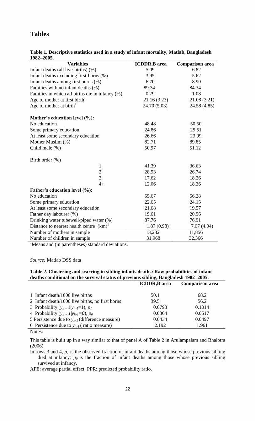
Table 1 presents sample means of the explanatory variables by area (percentages of
outcome 1 for dummy variables). The average number of children born per mother is 2.42 in the
ICDDR,B area and 2.73 in the comparison area; 19 per cent of families have more than three
children in the ICDDR,B area, compared with 29 per cent in the comparison area (these figures
are not reported in the Table). No differences between areas are observed in the mother’s average
age at birth. On average, mothers have lower education in the comparison area than in the
ICDDR,B area. In the comparison area, mothers less often have access to the more hygienic
sources of drinking water (tubewell/filter) and live much farther away from the nearest health
facility (7.1 versus 1.9 kilometres).
In the ICDDR,B area, 5.09 per cent of all live births result in infant death; 10.66 per cent
of all families experience at least one infant death and 0.79 per cent lose all their children in
infancy. Infant mortality among first-borns (6.70 per cent) is substantially higher than among
higher birth orders (3.95 per cent). In the comparison area, infant death is more common: 6.82
per cent of all children—8.90 per cent among first-borns; 5.62 per cent among higher birth
orders. Of all families, 15.66 per cent experienced at least one infant death and 1.08 per cent lost
all their children. Figure 1 presents the infant mortality rates by year of birth for both areas. It
shows a decreasing trend in both areas until the late nineties. The infant mortality rate has always
been higher in the comparison area than in the treatment area.
14
Table 2 shows the raw probabilities of infant death conditional on the survival status of
the preceding sibling. Explaining this was one of the primary goals of this study. The probability
of infant death is 4.34 percentage points (7.98 versus 3.64 per cent) if the preceding sibling dies
as an infant in the ICDDR,B area, and 4.97 percentage points in the comparison area (10.14
versus 5.17 per cent ). In other words, the likelihood of infant death is 2.2 (ICDDR,B area) or
twice as high (comparison area) if the preceding sibling dies than if it survives.
2.4 Model specification
The econometric model we used, which is similar to the models used by Arulampalam and
Bhalotra (2006, 2008) and Omariba et al. (2008), incorporates both scarring (state dependence)
and the potentially confounding effects of unobserved inter-family heterogeneity. The model
explains death during infancy of child t in family i. State dependence refers to whether the
survival status of the previous child (t-1) in the same family (i) has an influence on the survival
chances of the next child (t).
Let there be Ti children born alive in family i (i=1, 2,…,N – the number of families or
mothers in the sample); t=1, 2,…,Ti denotes birth order. For t>1, the unobserved propensity to
experience infant death yit* is specified as
yit* = x'itβ + γyit-1 + αi + uit , t=2,…, Ti (1)
The observed infant death outcome yit = 1 if the child’s propensity for death crosses a
threshold normalized to zero, that is, if yit* > 0; otherwise, if yit* ≤ 0, yit = 0 and the child does
not die in infancy. xit is a vector of strictly exogenous observed explanatory variables and β a
vector of coefficients; αi captures unobserved heterogeneity at the mother level, which remains
the same for all births of a given mother, accounting for all unobservable time-invariant
characteristics influencing the child’s propensity to die. The coefficient γ is associated with state
dependence. (In principle child t could die in infancy before child t-1 does, violating the
sequence of events assumed in our model. This never happens in our data and is therefore
ignored.) As in Omariba et al. (2008), the errors uit are assumed to follow a standard normal
distribution, independent of each other and of xis, s=1,…,Ti. In robustness checks in Section 7,
we also report results with logistic errors (following Arulampalam and Bhalotra 2006, 2008).
The model assumes that the history of infant deaths among older children other than the
immediately preceding child has no direct effect on yit*. For example, if child t-2 died in infancy,
in our model this will affect the risk of death of child t-1 and, thereby, also the risk of death of
child t, but there is no direct effect on death of child t. This is the first-order Markov assumption
(Zenger 1993; Arulampalam and Bhalotra 2006).
With the above specification, the conditional probability of death for infant t of mother i, given
yit-1, xit, and αi, is given by:
P[yit=1| yit-1, xit, αi ] = Φ [(x'itβ + γyit-1 + αi)], (2)

Chapter 2: Sibling death clustering
15
where Φ denotes the standard normal cumulative density. The joint conditional probability of the
observed sequence of binary outcomes is given by:
P(yi1,…….…., yi,T(i) | αi, xi1, …, xiT(i))
= P(yiT(i)|yiT(i)-1, αi, xiT(i))
× P(yi,T(i)-1|yi,T(i)-2, αi, xi,T(i)-1)
........................................
× P(yi2|yi1, αi, xi2) P(yi1| αi, xi1) (3)
Using the sequence above requires specifying P(yi1|αi,xi1) (the 'initial condition problem' in
dynamic models with unobserved heterogeneity; see Heckman, 1981; alternative approaches are
compared in a simulation study by Arulampalam and Stewart 2009 who conclude that the
various estimators perform similarly well).
Modelling the outcome of the first child is especially relevant because the first child shares
unobservable traits αi with its younger siblings. Without unobserved heterogeneity (αi=0 for all
i), the initial observation could be treated as exogenous, and equation (1) could be estimated
using the sample of second and further children only. Since the correlation between αi and yit-1
that makes yit-1 endogenous in equation (1) is probably positive, ignoring it would probably lead
to overestimation of γ (Fotouhi, 2005). This is why we specify a separate equation for mortality
of the first-born child. This equation has the same form as for equation (1) and is given by
yi1*= x'i1π + θαi + ui1 (4)
with the same assumptions for the error term ui1 as for the other uit. The auxiliary parameters π
and θ are estimated jointly with the parameters of interest. Exogeneity of first-child survival
corresponds to θ=0, which can be tested in a standard way. Equation (4) implies that the
conditional probability of infant death for the first-born child is given by:
P(yi1=1|αi, xi1) = Φ [x'i1π + θαi] (5)
Combining equations (1) and (4) gives the following conditional probability of an observed
sequence of binary outcomes yi1,…, yiT(i) for all children of family i:
P(yi1,yi2, ...yiT(i) |xiT(i),…, ,xi1, αi) =
Φ{(x'i1π + θαi)(2yi1–1)}Πt=2,…,T(i){Φ(x'itβ+γyit-1+αi)(2yit–1)} (6)

16
We assume that αi is normally distributed with mean 0 and variance σα2, independent of all xit
and uit , t=1,…,Ti . The likelihood contribution for family i is then given by
Li = ∫ P (yi1,yi2,...yiT(i)|xiT(i),…,xi1,α)ƒ(α) dα (7)
Where ƒ(α) is the density of N(0,σα2). The integral in (7) can be computed numerically
using Gauss-Hermite quadrature (Butler and Moffitt 1982). We used the Stata code of Stewart
(2007) to obtain the maximum likelihood estimates, based on 32 quadrature points.
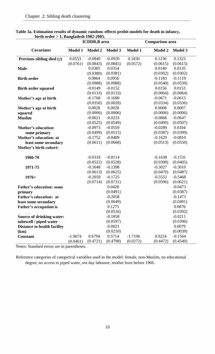
2.5 Estimation results
The estimates of several versions of the model are presented in Table 3a (equation (1), for birth
orders larger than 1) and Table 3b (equation (4), for first-borns). In Model 1, the only
explanatory variable is infant survival status of the previous sibling (yit-1); Model 2 adds child
and mother-level factors, and Model 3 also adds environmental and father-specific factors. We
estimated several model specifications, including models with dummies for birth order and
mother’s age at birth, and present the models that gave the best fit to the data, which is why some
background variables enter as dummies and others as continuous variables.
The estimates of γ for Model 1 imply that the death of the preceding sibling has a positive
significant effect on the probability of infant death in the comparison area, whereas a positive but
insignificant effect is found in the ICDDR,B area.
The partial effect of yit-1 on P[yit=1| yit-1, xit, αi ] can be derived from the estimates by
constructing counterfactual outcome probabilities p0, p1, fixing yit-1 at 0 and 1, evaluated at the
overall means of the exogenous variables and for αi = 0; the difference between p1 and p0 can
be interpreted as the average partial effect (APE); the ratio p1/p0 is the predicted probability ratio
(PPR) (Stewart 2007, p.522). Both are indicators of state dependence. In Model 1, the APE is
2.12 percentage points in the comparison area and 0.42 percentage points in the ICDDR,B area
(see Table 4). In terms of PPR, the likelihood of infant death is about 41 per cent greater if the
older sibling dies at infancy in the comparison area and about 12 per cent in the ICDDR,B area.
In the comparison area, including child and mother-level variables reduces the estimate
of γ and its significance level (Model 2); adding the father’s characteristics (Model 3) leads to a
small increase of γ and its significance level. In the ICDDR,B area, adding the regressors in
Models 2 and 3 leads to small negative and insignificant estimates of the scarring effect. In fact,
in the ICDDR,B area all three models find an insignificant scarring effect. Apparently, the
positive correlation between survival of consecutive children in the raw data (Table 2, lines 5 and
6) can be explained by observed and unobserved heterogeneity, leaving no significant role for
scarring. This may also mean that positive and negative scarring effects eliminate each other.
The predicted probability ratios (PPR) in Table 4 show that according to Model 3, the
likelihood of infant death in the comparison area is 29 per cent higher if the previous child dies at
infancy than if it survives. This effect is smaller than the estimate of Model 1, owing to the

Chapter 2: Sibling death clustering
17
inclusion of the covariates. Comparing the estimated scarring effect of 1.52 percentage points
with the differential of 4.97 percentage points in the raw data shows that in the comparison area,
scarring explains about one third of within-family clustering of infant deaths. The remaining part
is explained by observed and unobserved heterogeneity.
The estimates of θ in Table 3b can be used to test whether the initial outcome (infant
survival of the first child) can be treated as exogenous. If θ=0, the unobservables in equation (4)
would be uncorrelated with the unobservables in the main equation (1) and there would be no
need to estimate jointly the main equation (1) and the equation for the initial outcome (equation
(4)) (see Stewart, 2007, or Arulampalam and Bhalotra, 2006). The null hypothesis θ=0 is firmly
rejected for all our models in both areas. This confirms the importance of accounting for the
initial condition.
In Model 3, the proportion of the total unsystematic variance that is attributable to
family-level unobservables i is estimated to be 8.1 per cent in the comparison area and 22.2 per
cent in the ICDDR,B area (Table 3b). The null hypothesis of no family-level unobservables is
decisively rejected in both areas for all models, but unobserved heterogeneity plays a much
larger role in the ICDDR,B area than in the comparison area.
The other covariates often play different roles in the two areas and for first-born and non-
first-born children. Among first-born children, sons are more likely to die than daughters in both
areas, but the difference in the comparison area is smaller than in the ICDDR,B area. No
significant sex differences are observed for higher-birth orders. This is consistent with the results
of a study by Waldron (1983), who finds that infant mortality is inherently larger for boys than
for girls, but that this outcome can be reversed by environmental disadvantages for female
children. These environmental factors may be reduced by the extensive health services in the
ICDDR,B area.
In the ICDDR,B area, the probability of infant death has a U-shaped relationship with the
mother’s age at the time of childbirth, with a minimum at about age 30. In the comparison area,
the pattern is similar for first-born children but there is no evidence of increasing death
probabilities at older ages for higher-birth orders. The mother’s birth-cohort dummies indicate
significantly lower infant mortality probabilities for younger cohorts in both areas for first-born
and higher birth orders. This is probably because of a time trend in hygienic circumstances and
health technology, in line with the declining trends in Figure 1 and the findings of Arulampalam
and Bhalotra (2008). On the other hand, Omariba et al. (2008) found no significant effect of the
mother’s birth cohort.
In both areas, education of the mother significantly reduces the risk of infant mortality for
the first child, but not for higher birth orders once the father’s education is also controlled for
(Model 3). On the other hand, education of the father significantly reduces infant mortality of
higher birth orders but not of first-born children. Both education variables are measures of the
family’s socio-economic status, and the general conclusion is that higher socio-economic status

18
implies lower mortality. The third indicator of (low) socio-economic status is a dummy
indicating whether the father is a day labourer. As expected, it has a significantly positive effect
on mortality for higher birth orders, a finding similar to that of D’Souza and Bhuiya (1982); this
may reflect the association between high mortality and poor socio-economic conditions with
insecure household income. Mosley and Chen (1984) also relate this to the stable availability of a
basic minimum food supply of a variety sufficient to ensure adequate amounts of nutrients.
Those who used tubewell or pipe water as a source of drinking water are less likely to see
their children die in infancy, but this finding is significant for higher birth orders in the ICDDR,B
area only. The distance to the nearest health facility has a significantly positive effect on infant
mortality in the comparison area, and the effect is particularly pronounced for first-born children.
That no significant effect is found in the ICDDR,B area may be due to the fact that almost all
families live rather close to a health facility in that area.
A formal way to compare the results in the ICDDR,B area and the comparison area is
presented in the Annex to this chapter. Here the differential in mortality between the two areas is
decomposed into a part that can be ascribed to differences in the distribution of the covariates
and a residual part (ascribed to differences in parameters).
2.6 Alternative specifications and robustness checks
To analyse the sensitivity of our results to several specification choices, we estimated several
alternative models. Table 5 summarizes the main results, focusing on the estimates of the
scarring effect (γ). The first row reproduces the results from our benchmark model, Model 3 in
the previous section. To show the (upward) bias on the scarring effect when unobserved
heterogeneity is discarded, Row 2 presents the results of a simplified model without unobserved
heterogeneity. As expected, this leads to much higher estimates of the scarring effect: ignoring
unobserved heterogeneity implies that infant death clustering owing to unobserved heterogeneity
will incorrectly be attributed to scarring. This is exactly consistent with the explanation of
Arulampalam and Bhalotra (2006) for the necessity of incorporating both unobserved
heterogeneity and scarring in the same model (see also Section 2).
Row 3 adds the log birth interval as an additional regressor to the benchmark model. It
has a strong and significant negative effect on mortality, consistent with the existing literature.
Adding it leads to a smaller estimate of the scarring effect, which now has a different
interpretation: since birth intervals are kept constant, the scarring effect no longer includes the
(positive) effect through replacement and depletion (see Section 2). In other words, the
difference between the scarring effects in the benchmark model and the effects of the model with
the birth interval can be interpreted as an estimate of the effect through the mechanism that infant
mortality speeds up the next birth, and a faster next birth leads to a higher mortality risk. For the
comparison area, the estimated scarring effect in row 3 is virtually zero, so that the complete
scarring effect in the benchmark model works through the birth interval. For the ICDDR,B area,

Chapter 2: Sibling death clustering
19
the effect in row 3 is significantly negative, suggesting an effect of sibling competition or
learning (see Section 2).
Since Arulampalam and Bhalotra (2006, 2008) used logistic errors while Omariba et al.
(2008) used standard normal errors, we wanted to investigate the sensitivity of the results to this
choice. Row 4 replaces the normally distributed errors in the benchmark model by logistic errors.
The parameter estimates change owing to a different normalization (the variance of the error
terms is now π2/3 instead of 1), but significance levels and marginal effects are similar to those in
the benchmark model. This also applies to the other parameters of the model (details available on
request). Still, the estimated scarring parameter in the comparison area changes from marginally
significant (at the 5 per cent level) to marginally insignificant (p-value 0.062). In terms of log
likelihood, the probit model fits slightly better than the logit model, which is why we used probit
as the benchmark.
Finally, to obtain more efficient estimates, we combined the samples for the two areas,
tested whether the coefficients in the two areas were significantly different, and imposed equality
for sets of coefficients where supported by the test. This gives a more parsimonious version of
the model (which is not rejected against the benchmark model by a likelihood ratio test). The
final row of the table shows that the efficiency gain in the estimates of the scarring parameter
(which is significantly different in the two areas) is quite small. The standard errors and point
estimates hardly change compared to the benchmark.
In additional estimations, we also investigated interactions of the scarring effect with
other covariates (results not reported in the Table), but this did not lead to additional insights. For
example, interactions of the dummy for infant mortality of the previous child with educational
dummies were all insignificant, thus offering no evidence that scarring effects differ by
education level.
2.7 Discussion and conclusion
We analysed the determinants of infant mortality in Bangladesh in areas with and without health
services beyond the standard services provided by the government. We used recently developed
methods to account for heterogeneity across families as well as state dependence in infant
mortality. Our methods thus accounted for competing explanations for the stylized fact that a
child has a higher probability of death if the previous child of the same mother had died.
Separating the causal effect from unobserved heterogeneity has important implications for policy
in this area and for research on the inter-relationships of family behaviour and mortality. Indeed,
we find that controlling for unobserved heterogeneity is necessary to prevent substantial
overestimation of the causal 'scarring' effect of the death in infancy of the previous child.
We find that in the comparison area, the likelihood of infant death is almost 29 per cent
greater if the older sibling dies in infancy than if it survives. Adding the birth interval to the
model suggests that this scarring effect can be fully attributed to a mechanism that works through

20
birth intervals: infant death leads to a shorter next birth interval (replacement) and a shorter birth
interval increases mortality risk (nutritional depletion). In the ICDDR,B area, the same
mechanism plays a similar but smaller role, perhaps because of better health services and more
information on contraceptives and health risks. Moreover, it is offset by an effect of learning or
sibling competition in the opposite direction. The difference between scarring effects in the two
areas is consistent with the finding of Arulampalam and Bhalotra (2008) that (positive) scarring
is weaker in more developed regions.
Unobserved time-persistent heterogeneity among mothers captures 22 per cent of the
total unsystematic variation in infant deaths in the ICDDR,B area, compared to only 8 per cent in
the comparison area. An explanation may be that some mothers who receive health information
are better at exploiting this than others, so that additional health information increases
heterogeneity. Another explanation might be that the ICDDR,B area is divided into four sub-
regions ('blocks'), with interventions such as vaccinations phased out at different times in
different blocks, so that different children benefit differently from these interventions; dummies
for whether specific interventions were introduced at the time of birth were not significant,
however, so that this explanation could not be confirmed. Echoing the results of Hale et al.
(2006), we do find that the effect of the mother’s birth cohort is stronger in the ICDDR,B area
than in the comparison area, possibly reflecting the advantages of introducing extensive health
services in the ICDDR,B area.
Estimating the model for the higher educated mothers only (results not reported) suggests
that the mother-specific variation in infant deaths is 16 per cent greater among mothers with
secondary or higher education than for the complete ICDDR,B sample. This finding confirms the
prediction that “the new interventions will tend to increase the inequality since they will initially
reach those who are already better off” (Victora et al. 2001; Razzaque et al. 2007). On the other
hand, in the comparison area, greater unobserved heterogeneity is observed among mothers with
no education level, possibly owing to variation in innate ability (Das Gupta 1990).
Our findings confirm the general result that low socio-economic status increases the risk
of infant death, but we find some remarkable and policy-relevant differences between first-born
and later-born children. For the first-born, the mother’s education seems particularly important,
suggesting that it is particularly difficult for low educated first-time mothers to create a healthy
environment for a newborn child. At the time of first birth, education may improve the women’s
autonomy and decision making; a woman’s autonomy is lowest when she is a young mother, and
education helps women to overcome the barriers imposed by low autonomy in a traditional
society (Das Gupta 1990). For higher birth orders where competition among siblings for scarce
resources matters, the father’s education seems more important, possibly as an indicator of the
family’s general socio-economic status. A longer distance to the nearest health facility leads to
higher mortality in the comparison area and this effect is more pronounced for the first-born
child than for children of higher birth order, possibly reflecting the social taboos restricting the
mobility of younger mothers. The effect of safe drinking water in the ICDDR,B area—a finding

Chapter 2: Sibling death clustering
21
unique among studies of death clustering—is consistent with the discussion in the background
section.
We believe our findings can contribute to the formulation of effective policies targeted at
achieving the fourth millennium development goal of reducing under-five mortality. The
differences between the two areas highlight the important role of extensive maternal and child
health interventions: the kind of extensive health services and health information available in the
ICDDR,B area. Of particular note is the fact that in the ICDDR,B area we find some families that
appear to have learnt from the experience of infant death in the past how to reduce the
probability of the death of the next child. On the other hand, the finding that unobserved
heterogeneity in the ICDDR,B area is much greater than in the comparison area implies that not
everyone benefits equally from the health interventions, which suggests that policies that
increase equity in the use of interventions may help to reduce infant mortality further.
22
Tables
Table 1. Descriptive statistics used in a study of infant mortality, Matlab, Bangladesh
1982–2005.
Variables ICDDR,B area Comparison area
Infant deaths (all live-births) (%) 5.09 6.82
Infant deaths excluding first-borns (%) 3.95 5.62
Infant deaths among first borns (%) 6.70 8.90
Families with no infant deaths (%) 89.34 84.34
Families in which all births die in infancy (%) 0.79 1.08
Age of mother at first birth1 21.16 (3.23) 21.08 (3.21)
Age of mother at birth1
24.70 (5.03) 24.58 (4.85)
Mother’s education level (%):
No education 48.48 50.50
Some primary education 24.86 25.51
At least some secondary education
26.66 23.99
Mother Muslim (%) 82.71 89.85
Child male (%) 50.97 51.12
Birth order (%)
1 41.39 36.63
2 28.93 26.74
3 17.62 18.26
4+ 12.06 18.36
Father’s education level (%):
No education 55.67 56.28
Some primary education 22.65 24.15
At least some secondary education 21.68 19.57
Father day labourer (%) 19.61 20.96
Drinking water tubewell/piped water (%) 87.76 76.91
Distance to nearest health centre (km)1 1.87 (0.98) 7.07 (4.04)
Number of mothers in sample 13,232 11,856
Number of children in sample 31,968 32,366 1Means and (in parentheses) standard deviations.
Source: Matlab DSS data
Table 2. Clustering and scarring in sibling infants deaths: Raw probabilities of infant
deaths conditional on the survival status of previous sibling, Bangladesh 1982–2005.
ICDDR,B area Comparison area
1 Infant death/1000 live births 50.1 68.2
2 Infant death/1000 live births, no first borns 39.5 56.2
3 Probability (yit = 1|yit-1=1), p1 0.0798 0.1014
4 Probability (yit = 1|yit-1=0), p0 0.0364 0.0517
5 Persistence due to yit-1 (difference measure)
(row 3- row 4), APE
0.0434 0.0497
6 Persistence due to yit-1 ( ratio measure)
(row 3/row 4), PPR
2.192 1.961
Notes:
This table is built up in a way similar to that of panel A of Table 2 in Arulampalam and Bhalotra
(2006).
In rows 3 and 4, p1 is the observed fraction of infant deaths among those whose previous sibling
died at infancy; p0 is the fraction of infant deaths among those whose previous sibling
survived at infancy.
APE: average partial effect; PPR: predicted probability ratio.
Chapter 2: Sibling death clustering
23
Table 3a. Estimation results of dynamic random–effects probit models for death in infancy,
birth order > 1, Bangladesh 1982-2005.
Covariates
ICDDR,B area Comparison area
Model 1 Model 2 Model 3 Model 1 Model 2 Model 3
Previous sibling died (γ) 0.0553
(0.0761)
-0.0840
(0.0843)
-0.0920
(0.0845)
0.1830
(0.0572)
0.1236
(0.0615)
0.1323
(0.0615)
Male 0.0385
(0.0380)
0.0354
(0.0381)
0.0140
(0.0302)
0.0135
(0.0302)
Birth order 0.0864
(0.0988)
0.0956
(0.0988)
-0.1183
(0.0540)
-0.1119
(0.0539)
Birth order squared -0.0149
(0.0133)
-0.0152
(0.0133)
0.0156
(0.0064)
0.0153
(0.0064)
Mother’s age at birth -0.1768
(0.0350)
-0.1690
(0.0028)
-0.0671
(0.0334)
-0.0615
(0.0336)
Mother’s age at birth
squared
0.0028
(0.0006)
0.0028
(0.0006)
0.0008
(0.0006)
0.0007
(0.0006)
Muslim -0.0621
(0.0525)
-0.0233
(0.0549)
-0.0866
(0.0490)
-0.0647
(0.0507)
Mother’s education:
some primary
-0.0973
(0.0499)
-0.0559
(0.0515)
-0.0289
(0.0387)
0.0104
(0.0399)
Mother’s education: at
least some secondary
-0.1752
(0.0611)
-0.0489
(0.0668)
-0.1629
(0.0513)
-0.0810
(0.0550)
Mother’s birth cohort:
1966-70 -0.0318
(0.0522)
-0.0114
(0.0528)
-0.1638
(0.0398)
-0.1531
(0.0405)
1971-75 -0.1648
(0.0613)
-0.1398
(0.0625)
-0.3027
(0.0470)
-0.3010
(0.0487)
1976+ -0.2059
(0.0714)
-0.1725
(0.0731)
-0.5552
(0.0596)
-0.5468
(0.0621)
Father’s education: some
primary
0.0428
(0.0491)
-0.0473
(0.0387)
Father’s education: at
least some secondary
-0.2058
(0.0649)
-0.1473
(0.0491)
Father’s occupation is
day labourer
0.1275
(0.0516)
0.0876
(0.0392)
Source of drinking water:
tubewell / piped water
-0.1858
(0.0597)
-0.0211
(0.0396)
Distance to health facility
(km)
-0.0021
(0.0210)
0.0079
(0.0039)
Constant -1.9674
(0.0461)
0.6794
(0.4721)
0.5714
(0.4798)
-1.7106
(0.0272)
0.0224
(0.4472)
-0.1564
(0.4540)
Notes: Standard errors are in parentheses.
Reference categories of categorical variables used in the model: female, non-Muslim, no educational
degree, no access to piped water, not day labourer, mother born before 1966.
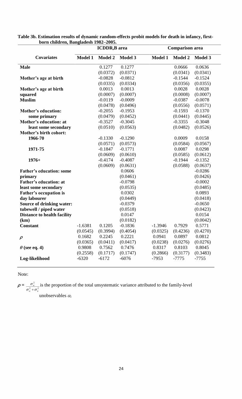
24
Table 3b. Estimation results of dynamic random-effects probit models for death in infancy, first-
born children, Bangladesh 1982–2005.
Covariates
ICDDR,B area Comparison area
Model 1 Model 2 Model 3 Model 1 Model 2 Model 3
Male 0.1277
(0.0372)
0.1277
(0.0371)
0.0666
(0.0341)
0.0636
(0.0341)
Mother’s age at birth -0.0828
(0.0335)
-0.0812
(0.0334)
-0.1544
(0.0356)
-0.1524
(0.0355)
Mother’s age at birth
squared
0.0013
(0.0007)
0.0013
(0.0007)
0.0028
(0.0008)
0.0028
(0.0007)
Muslim -0.0119
(0.0478)
-0.0009
(0.0496)
-0.0387
(0.0556)
-0.0078
(0.0571)
Mother’s education:
some primary
-0.2055
(0.0479)
-0.1953
(0.0452)
-0.1593
(0.0441)
-0.1370
(0.0445)
Mother’s education: at
least some secondary
-0.3527
(0.0510)
-0.3045
(0.0563)
-0.3355
(0.0482)
-0.3048
(0.0526)
Mother’s birth cohort:
1966-70 -0.1330
(0.0571)
-0.1290
(0.0573)
0.0009
(0.0584)
0.0158
(0.0567)
1971-75 -0.1847
(0.0609)
-0.1771
(0.0610)
0.0087
(0.0585)
0.0298
(0.0612)
1976+ -0.4174
(0.0609)
-0.4087
(0.0631)
-0.1944
(0.0588)
-0.1352
(0.0637)
Father’s education: some
primary
0.0606
(0.0461)
-0.0286
(0.0426)
Father’s education: at
least some secondary
-0.0798
(0.0535)
-0.0002
(0.0485)
Father’s occupation is
day labourer
0.0302
(0.0449)
0.0893
(0.0418)
Source of drinking water:
tubewell / piped water
-0.0379
(0.0518)
-0.0650
(0.0423)
Distance to health facility
(km)
0.0147
(0.0182)
0.0154
(0.0042)
Constant -1.6381
(0.0545)
0.1205
(0.3994)
-0.1836
(0.4054)
-1.3946
(0.0325)
0.7929
(0.4236)
0.5771
(0.4270)
0.1682
(0.0365)
0.2245
(0.0411)
0.2221
(0.0417)
0.0941
(0.0238)
0.0897
(0.0276)
0.0812
(0.0276)
θ (see eq. 4) 0.9808
(0.2558)
0.7562
(0.1717)
0.7476
(0.1747)
0.8317
(0.2866)
0.8103
(0.3177)
0.8045
(0.3483)
Log-likelihood -6320 -6172 -6076 -7953 -7775 -7755
Note:
= 22
2
u
is the proportion of the total unsystematic variance attributed to the family-level
unobservables i

Chapter 2: Sibling death clustering
25
Table 4. Average predicted probabilities of infant death given previous sibling’s survival status,
Bangladesh 1982–2005.
Probabilities
ICDDR,B area Comparison area
Model 1 Model 2 Model3 Model 1 Model 2 Model 3
P1 0.0406 0.0335 0.0321 0.0730 0.0678 0.0681
P0 0.0364 0.0394 0.0384 0.0518 0.0536 0.0530
APE: p1- p0 0.0042 -0.0059 -0.0063 0.0212 0.0141 0.0152
PPR: p1/p0 1.116 0.850 0.836 1.410 1.263 1.286
Notes: p1 is computed using the estimated marginal predicted probability of yit for each observation
under the condition that the previous sibling died (yit-1 = 1), averaged over all observations (with t
>1). Similarly, p0 is obtained setting yit-1 = 0.
APE: average partial effect; PPR, predicted probability ratio.
Table 5. Scarring parameter (γ) and log likelihoods of alternative specifications of models
estimating infant mortality, Bangladesh 1982–2005.
ICDDR,B area Comparison area
Estimate of γ
(standard
error)
Log likelihood Estimate of γ
(standard error)
Log
likelihood
Benchmark model
(Table 3, Model 3)
-0.092
(0.084)
-6153.10 0.132*
(0.061)
-7755.52
No unobserved
heterogeneity
0.296**
(0.051)
-6173.83 0.276**
(0.044)
-7757.00
With log birth
interval
-0.181*
(0.082)
-6145.42 -0.009
(0.069)
-7742.60
Logit model -0.140
(0.151)
-6153.11 0.230
(0.123)
-7757.88
Joint estimation
both areas
-0.037
(0.074)
-13,922.75+
0.121
(0.062)
Notes:
*p–value < 0.05; ** p–value < 0.01
+: log likelihood of joint model, imposing equality of 22 slope coefficients in the two areas.
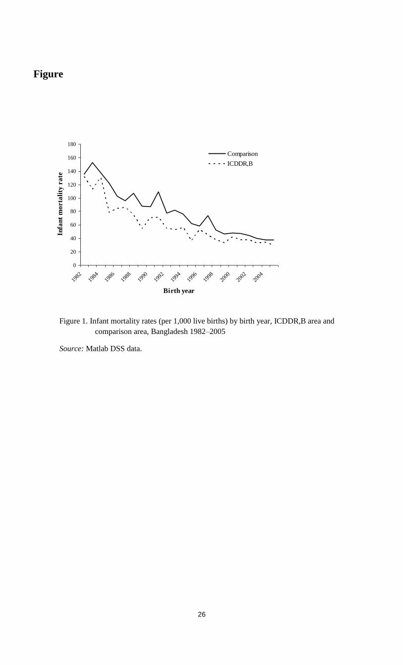
26
Figure
0
20
40
60
80
100
120
140
160
180
1982
1984
1986
1988
1990
1992
1994
1996
1998
2000
2002
2004
Birth year
Infa
nt
mo
rta
lity
ra
te
Comparison
ICDDR,B
Figure 1. Infant mortality rates (per 1,000 live births) by birth year, ICDDR,B area and
comparison area, Bangladesh 1982–2005
Source: Matlab DSS data.

Chapter 2: Sibling death clustering
27
Annex
Decomposing the Difference between Areas
The aggregate prediction of the infant mortality rate according to model 3 for all children (first
born as well as others) is about 49 per thousand live births in the ICDDR,B area and 67 per
thousand live births in the comparison area, a difference of 18 per thousand live births. We
analyze the gap between the two areas using the common technique of decomposing differences
in mean levels into those due to different observable characteristics or “endowments” and those
due to different effects of characteristics or “coefficients” (Blinder 1973; Oaxaca 1973). In the
standard case of a linear model the technique requires coefficient estimates from linear
regressions for the outcome of interest and sample means of the independent variables used in
the regressions. Adjustments for the case of a nonlinear model such as our binary choice model
were introduced by Fairlie (2005) and Yun (2004).
Here we follow the decomposition methodology proposed by Yun (2004) for the probit
model (binary dependent variable), which can straightforwardly be extended to the dynamics
random effects probit model taking into account of the initials conditions and the unobserved
heterogeneity. The ‘aggregate’ or ‘overall’ mean difference in infant mortality between the two
areas ICDDR,B (group A) and comparison (group B) can be decomposed as follows:
( ) ( )
( ) ( )
A B A A A A B A A B
B A A B B B B B
Y Y X X
X X
(1)
The means are taken over either all first born children or all higher birth orders of all
mothers in each area and over the random effects. We have used shorthand notation, dropping
indexes i and t and combining expressions for the first born child and the second and higher birth
orders. For example, AX includes itx as well as 1ity for t>1, A denotes either (for birth
order 1) or ( , ) (for higher birth orders), and or 1 for birth order equal to 1 or larger
than 1, respectively.
The first component in the decomposition in equation (1) is the “endowment” or
“composition effect”, the part of the difference explained by differences in (observed and
unobserved) characteristics of in the two samples. The second is the residual difference keeping
characteristics constant. To estimate the two components, we replace the parameters by the
estimates for Model 3 in Table 3 for the treatment area (A) or the comparison area (B). This is
referred to as decomposition 1. We also present the results in the reverse order, i.e., taking the
comparison area as group A and the treatment area as group B (and adding minus signs for

28
comparability), which we refer to as decomposition 2. The unobserved heterogeneity terms are
replaced by random draws from their estimated normal distributions.
To understand which characteristics contribute to explaining the mortality difference between the
two regions, we also performed the so-called detailed decomposition, again following Yun
(2004). For this purpose, equation (1) is rewritten as follows:
1
1
( ) ( )
( ) ( )
i ki
A B x A A A A B A A B
i
i ki
B A A B B B B B
i
Y Y W X X
W X X
(2)
Where the “weights” are given by
iW =
i ii
A B A
A B A
X X
X X
and
iW =
i i i
A B B
A B B
X
X
, so that
ki
i
i
xW1
=
ki
i
iW1
=1.
We focus on the contribution of each variable to the endowment effect, the first part in
(2). We present the results for the second part for completeness, but we do not have a good
interpretation for these in our context.
The bottom rows of the two panels in Table A give the results of the overall
decomposition (for Model 3) (“Total”). For the first born child, almost two thirds of the mortality
gap is explained by characteristics according to both decomposition 1 and decomposition 2 (16.3
or 17.0 per one thousand live births, of a total gap of 24.9 per thousand live births). The detailed
composition shows that this is almost completely due to the variable distance to the nearest
health facility. This variable has a strong (negative) effect on survival chances and the distances
are much larger in the comparison area than in the treatment area.
For higher birth orders, differences in characteristics explain a smaller part of the total
gap and the results are sensitive to which of the two decompositions is used. According to
decomposition 2, the endowment effect is about one third of the total effect (5 out of the total
gap of 15 per thousand live births) and again this is mainly driven by the distance to the nearest
health facility, though mother’s age at birth also plays a role: mortality falls with age of the
mother at birth, and mothers in the treatment area are somewhat older, on average. According to
decomposition 1, however, the difference in distance to a health facility hardly plays a role. The
reason is that this is now weighted by the coefficient estimate for the distance variable in the
treatment area, which is small and insignificant. Accordingly, decomposition 1 also attributes a
much smaller contribution to all observed differences in characteristics (1.5 out of 15).
Chapter 3
Reproductive Behaviour and Infant Deaths:
Causal Analysis2
3.1 Introduction
According to the demographic transition theory, there is a strong correlation between childhood
mortality and fertility. Empirical evidence has shown that a decline in childhood mortality is
often a prerequisite for fertility decline (Chowdhury et al. 1976; Matthiesson and McCann 1978;
Pritchett 1994; Wolpin 1997). Other studies have emphasized the reverse direction of this
causation, e.g., high fertility and the close birth-spacing associated with it cause an increase in
child mortality (Cleland and Sathar 1984; Curtis et al. 1993). Yet another set of studies
emphasized that the analysis of the direction of causality with birth interval data is hampered by
the close interrelations between child mortality and fertility (Zimmer 1979; Santow and Bracher
1984).
Studies have emphasized that the observed associations between child mortality, birth
spacing, and fertility can be due to various causal mechanisms, but may also be explained by
common unobserved factors that drive the various processes. From the point of view of policies
aimed at optimal birth spacing, reducing mortality, and reducing fertility, it is crucial to identify
the importance of the various causal mechanisms and alternative explanations. If associations
reflect spurious correlation or reverse causation, then the implications for policy design can be
dramatically altered (Moffitt 2005). Ben-Porath (1976, p. S168) already argued that in micro
data, associations may not reflect causal effects but may be spurious and reflect left-out variables
operating simultaneously on fertility and mortality. In addition, a recent study conducted by
DaVanzo and her colleagues (DaVanzo et al. 2008) in Matlab emphasized the importance for
joint analysis including interval lengths and mortality, allowing for correlated risks among
different births to the same mother.
To achieve this latter goal, we use a panel data model similar to the one introduced by
Bhalotra and van Soest (2008). This model incorporates various causal mechanisms as well as
2 This chapter is joint work with Arthur van Soest, Tilburg University. This paper has been presented in the Statistics
and Econometrics seminar, Tilburg University. We thank seminar participants and members of the committee for
helpful comments and suggestions.

30
unobserved heterogeneity, exploiting the sequence of all births and deaths to a mother to
accommodate the correlations between mortality risks of consecutive children and birth intervals.
Equations driving the processes of infant mortality, birth spacing, and fertility are estimated
jointly to account for the various sources of endogeneity. Each of the equations incorporates a
mother specific unobserved heterogeneity term. The estimates of the causal parameters therefore
remain consistent in the presence of reverse causality or unobserved heterogeneity. The model
has an equation for mortality (neonatal mortality in Bhalotra and van Soest; infant mortality in
our study), for the birth interval, and for the decision to have another birth. Mortality depends on,
among other things, the length of the preceding birth interval (for birth orders higher than one),
age of the mother, gender of the child, socio-economic status of the family, religion, and an
unobserved mother specific effect. The decision whether to have another child or not and the
birth interval after a given birth until the next birth in turn depend on gender and survival status
of previously born children, age of the mother, socio-economic status, religion, and unobserved
mother-specific effects. The three mother-specific unobserved effects are allowed to be
correlated to capture the possibility of common unobserved factors driving the various processes.
The model is estimated with maximum likelihood, accounting for all the correlations and for
censoring in the birth spacing equation (fertility may be incomplete at the end of the observation
window).
In contrast to Bhalotra and van Soest (2008), who uses retrospective data from the Indian
Demographic and Health Survey, we use prospective data from the Demographic and Health
Surveillance System, Matlab, Bangladesh, following mothers residing in the study area over time.
This has the advantage that several covariates, such as indicators of socio-economic status and
environmental factors such as availability of drinking water) are observed at the relevant points
in time when children are born (rather than at survey time in the retrospective data). Moreover, it
avoids recall error in, for example, the dates when children were born. A second feature that is
specific to our data is that the study area is randomly split into villages with standard government
provided health services: the comparison area and villages with additional extensive health
services, such as more health clinics and regular visits of health officers: the ICDDR,B area or
treatment area (Bhatia 1983; Van Ginneken et al. 1998). Comparing the model estimates for the
two areas gives insight in how the extensive health services influence affect birth spacing,
mortality, and fertility and the various relations between these processes.
3.2 Overview of causal mechanisms
According to the classical demographic transition theory, child mortality affects fertility in two
ways: physiological/biological changes and behavioral/replacement effects. The physiological
effect can be explained by the fact that breastfeeding is interrupted with a child death, and
consequently, the postpartum infecundable period is shortened (Van Ginneken 1974; Mondot-
Bernard 1977; Knodel 1978). As a result under ineffective use or non-use of contraception, the
mother is able to conceive the next child sooner, leading to a shorter birth interval and, possibly,
higher fertility. The effect of child mortality on birth intervals is closely linked to the influence
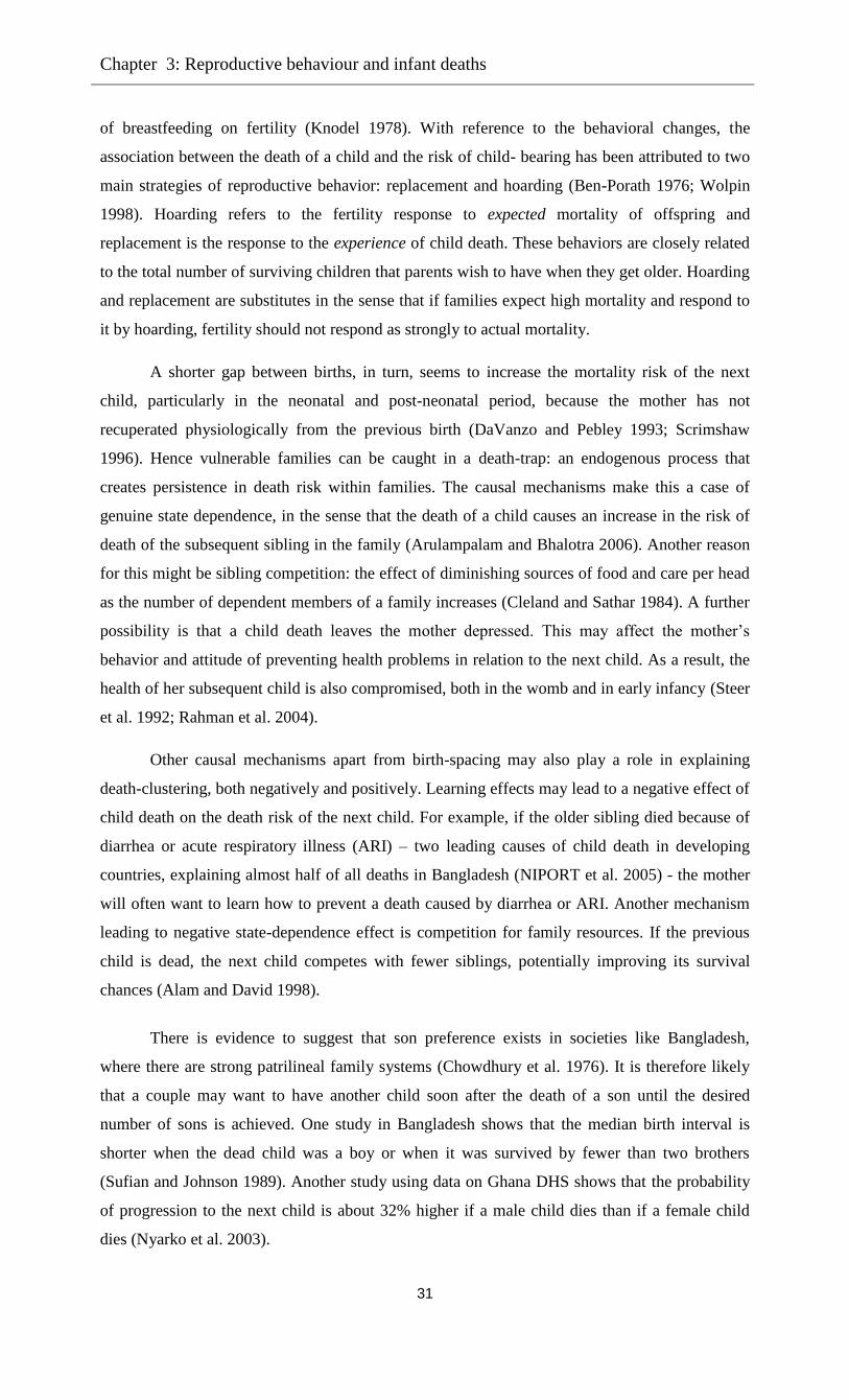
Chapter 3: Reproductive behaviour and infant deaths
31
of breastfeeding on fertility (Knodel 1978). With reference to the behavioral changes, the
association between the death of a child and the risk of child- bearing has been attributed to two
main strategies of reproductive behavior: replacement and hoarding (Ben-Porath 1976; Wolpin
1998). Hoarding refers to the fertility response to expected mortality of offspring and
replacement is the response to the experience of child death. These behaviors are closely related
to the total number of surviving children that parents wish to have when they get older. Hoarding
and replacement are substitutes in the sense that if families expect high mortality and respond to
it by hoarding, fertility should not respond as strongly to actual mortality.
A shorter gap between births, in turn, seems to increase the mortality risk of the next
child, particularly in the neonatal and post-neonatal period, because the mother has not
recuperated physiologically from the previous birth (DaVanzo and Pebley 1993; Scrimshaw
1996). Hence vulnerable families can be caught in a death-trap: an endogenous process that
creates persistence in death risk within families. The causal mechanisms make this a case of
genuine state dependence, in the sense that the death of a child causes an increase in the risk of
death of the subsequent sibling in the family (Arulampalam and Bhalotra 2006). Another reason
for this might be sibling competition: the effect of diminishing sources of food and care per head
as the number of dependent members of a family increases (Cleland and Sathar 1984). A further
possibility is that a child death leaves the mother depressed. This may affect the mother’s
behavior and attitude of preventing health problems in relation to the next child. As a result, the
health of her subsequent child is also compromised, both in the womb and in early infancy (Steer
et al. 1992; Rahman et al. 2004).
Other causal mechanisms apart from birth-spacing may also play a role in explaining
death-clustering, both negatively and positively. Learning effects may lead to a negative effect of
child death on the death risk of the next child. For example, if the older sibling died because of
diarrhea or acute respiratory illness (ARI) – two leading causes of child death in developing
countries, explaining almost half of all deaths in Bangladesh (NIPORT et al. 2005) - the mother
will often want to learn how to prevent a death caused by diarrhea or ARI. Another mechanism
leading to negative state-dependence effect is competition for family resources. If the previous
child is dead, the next child competes with fewer siblings, potentially improving its survival
chances (Alam and David 1998).
There is evidence to suggest that son preference exists in societies like Bangladesh,
where there are strong patrilineal family systems (Chowdhury et al. 1976). It is therefore likely
that a couple may want to have another child soon after the death of a son until the desired
number of sons is achieved. One study in Bangladesh shows that the median birth interval is
shorter when the dead child was a boy or when it was survived by fewer than two brothers
(Sufian and Johnson 1989). Another study using data on Ghana DHS shows that the probability
of progression to the next child is about 32% higher if a male child dies than if a female child
dies (Nyarko et al. 2003).

32
Observed clustering in infant or child mortality of successive children may be due to birth
interval effects but also to some other factors. Most studies of birth spacing and childhood
mortality do not appropriately control for whether the previous child died or survived as well as
unobserved heterogeneity. Exceptions are Arulampalam and Bhalotra (2006) in India and
Omariba et al. (2008) in Kenya. Findings from these studies reveal that the causal effect of
previous mortality is overestimated when unobserved heterogeneity is not accounted for.
3.3 Literature review
Several researchers have investigated the relationship between child mortality and fertility,
especially in developing countries, and have demonstrated firm evidence of an increased
probability of pregnancy among women who lost their child (for example, Harrington 1971;
Chowdhury et al. 1976; Ben-Porath 1976; Park et al. 1998). In Bangladesh, Chowdhury et al.
find that infant death shortened median birth interval from 37.2 to 24.1 months. A study in
Ghana shows that the death of the previous child shortens the length of interval by 11 months
and confirms that the parity progression ratio is higher if an infant dies than if it survives
(Nyarko et al. 2003). Ben-Porath (1976) studied Jewish women born in Asia or Africa and a
group of women born in Europe or America or Israel and found significant replacement effects.
Bhalotra and van Soest (2008) suggest that for every neonatal death in India, 0.37 extra children
are born.
On the other hand, studies investigating effects of birth-spacing on mortality have
observed a close association between a short preceding birth-interval and mortality (Zenger
1993; Guo 1993; Miller et al. 1992; Koenig et al. 1990; Alam and David 1998), and this
association has been observed to be stronger when the preceding sibling survived compared to
when it died (Zenger 1993; Koenig et al. 1990; Alam and David 1998). This may imply that the
birth interval effect on mortality is confounded by the association between the mortality risks of
successive births. In Bangladesh Demographic and Health Survey 2007 (NIPORT et al. 2008)
the percentage of births that occur within a very short interval (less than 18 months) is six times
higher for children whose prior sibling died than for those whose prior sibling survived.
Multivariate analyses with large datasets from a number of different settings suggest that birth-
intervals of at least three years are associated with better health outcomes for children (Conde-
Agudelo et al. 2006; DaVanzo et al. 2004; Rutstein 2005).
Based on Matlab data, DaVanzo et al. (2008) report how detrimental effects of short birth
intervals vary by pregnancy outcomes. For mortality in the first week of a child’s life, they find
that birth interval effects are greater if the sibling born at the beginning of the birth interval died
than if it survived. After one month, however, the effects are greater if the previously born
sibling was still alive. Their findings are in the line with the maternal depletion hypothesis and
with sibling competition. However, in their analysis they did not account for endogeneity in the
birth spacing or for correlated risks of death among different births of the same mother. In their
Chapter 3: Reproductive behaviour and infant deaths
33
conclusions they emphasized that this remains a significant area for future research using Matlab
data, and this is in essence the contribution of this paper.
3.4 Policy implications Understanding the mechanisms of causality will help policymakers to determine how to allocate
limited resources for effective interventions. For example, scarring effects can explain that the
death of a previous child increases the death risk of the next child. In the patriarchal society of
Bangladesh where son preference is very high (Chowdhury et al. 1990), it is expected that the
scarring effects are higher if the deceased child was a boy and the index child is a daughter. If
this appears to be the case, policymakers can pay more attention to a gender discrepancies
campaign at the national level or can launch a female empowerment program, educating females
up to a certain level. Another example can be derived from the relationship between birth-
spacing and child mortality, especially neonatal or post-neonatal mortality, due to mother’s
depletion. If this is important, policy makers can focus on birth-intervals and start campaigning
to promote a minimum birth-interval that will enable mothers to recuperate physiologically from
child birth and prepare them for future births.
Furthermore, if we find that mother-specific effects are important, this may suggest that
women who have experienced the loss of a child will be at higher risk of losing a second or third
child. It can also help us to understand how a particular intervention (e.g. safe drinking-water)
affects other components of health. For example, safe drinking-water was supplied to reduce
childhood mortality but in reducing child mortality it also may help to lower the total fertility
rate and hence may, in turn, also increase the birth-spacing between two births, giving more
insight in how these particular mechanisms work.
3.5 Data
3.5.1 Study sample
Since 1966 ICDDR,B maintained a Health and Demographic Surveillance System (HDSS) in
Matlab, aiming to support the Health and Family Planning programme in Bangladesh. Matlab is
an area located in 60 km southeast of Dhaka in which all births, deaths, causes of deaths (through
verbal autopsy), pregnancy histories, migrations in and out of the area, marriages, divorces, and
several indicators of socioeconomic status are recorded for the complete population of about
220,000 people.3 The HDSS data on the timing of pregnancy outcomes and deaths are thought to
be of very high quality because they have been collected during regular visits (every two weeks
until the late 1990s and every month since then) by well-trained female community health
workers (CHWs; see, e.g., D’Souza 1981 or van Ginneken et al. 1998). We combined the health
and demographic surveillance system data from 70 villages in the ICDDR,B area and 79 villages
3 For details on surveillance system, see chapter 2 or Saha and van Soest (2011).

34
in the comparison area obtained from 1 July, 1982 until 31 December, 2005 (the study period).
Data from before 1 July 1982 have not (yet) been made available for research.
The complete data set has records on about 63,000 mothers, with more than 165,000 child
births – including live singleton births, multiple births, and still births. For our purposes, we
selected a subsample of mothers without multiple births4
and with complete5
live birth
information who were continuously living in the Matlab area since the birth of their first child.
This implies that we deleted mothers who migrated out of Matlab during the period under study.
Moreover, we discarded stillbirths.6 Finally, we have excluded the children born in three
villages which shifted from the ICDDR,B area to the comparison area in 2000. This leads to
working samples of 31,968 children and 13,232 mothers in the ICDDR,B area and 32,366
children and 11,856 mothers in the comparison area.
3.5.2 Variables and descriptive statistics
Table 1 presents sample means (percentages of outcome 1 for dummy variables) by area. In the
ICDDR,B area, 5.09 percent of all live births resulted in infant death; 10.66 percent of all
families experienced at least one infant death and 0.79 percent lost all their children in infancy.
The percent of infant death among first born is 6.70, substantially higher than among children of
higher birth order (3.95 percent). In the comparison area, infant death was more common: 6.82
percent of all children where 8.90 percent among first born; 5.62 percent among higher birth
orders. Of all families, 15.66 per cent experienced at least one infant death and 1.08 per cent lost
all their children. About 20.6% birth intervals are shorter than or equal to 24 months in the
comparison area, compared to about 12.9 % in the ICDDR,B area.
The average number of children born per mother is 2.42 in the ICDDR,B area and 2.73 in
the comparison area; 19 percent of families had more than three children in the ICDDR,B area,
compared to 29 percent in the comparison area (not reported in the table). No differences
between areas are observed in the mother’s average age at birth. Mothers have a somewhat lower
education level in the comparison area than in the ICDDR,B area, on average. In the comparison
area, mothers less often have access to the more hygienic source of drinking water
(tubewell/filter) and live much farther away from the nearest health facility (7.1 kilometres on
average, compared to 1.9 kilometres in the ICDDR,B area).
Figure 1, based upon non-parametric regressions of infant mortality on the preceding
birth interval, depicts a sharp decline in infant mortality rates when birth intervals increase in
both ICDDR,B and comparison area. At short birth intervals, the probability of infant death is
4 We eliminated multiple births as children of a multiple birth face much higher odds of dying requiring a separate
analysis, as has been documented in the demographic literature. 5 To have a mother’s complete birth information during the study period we have calculated parity (total number of
live births) from the pregnancy history variables. We have checked parity and birth dates of all children. For
example, if a mother has parity four, this means this mother has had four live births, so the birth dates of four
children should be available in the file and this mother will appear four times as giving birth. If this was not the case
(e.g., if a child was born outside of the Matlab area or before study period or deleting multiple births may caused
incomplete birth information of a mother), we have deleted all children’s records of this mother. 6 One reason why we eliminated stillbirths is that gender, an important covariate in our analysis, is missing for
stillbirths. We define birth intervals as intervals between reported dates of live births, ignoring stillbirths in between
live births

Chapter 3: Reproductive behaviour and infant deaths
35
highest, and it falls with birth interval length until an interval length of about 4.5 years
(exp(4)=54 months). Particularly in the ICDDR,B area, the survival chances are quite stable and
even seem to increase a little when birth intervals increase beyond 4.5 years. This pattern is in
line with the wide demographic literature on this issue; see, for example, Figure 1 in Bhalotra
and van Soest (2008).
Figures 2 and 3 show the distributions of the log birth interval by survival status of the
previous child and gender in the ICDDR,B area and the comparison area. In both areas, there is a
large difference in the distributions of the birth interval after infant death and after infant survival.
This difference is much larger than the difference in the Indian state Uttar Pradesh found by
Bhalotra and van Soest (2008, Figure 2). In the ICDDR,B area, the median birth intervals are 20
months after an infant death and 48 months otherwise (averages are 23 and 51 months). They are
17 and 37 months (averages are 22 and 42 months) in the comparison area. However, no
significant difference is observed in these distributions by survival status and gender.
3.6 Model Specification
In this section we present the econometric model. This is similar to the model in Bhalotra and
van Soest (2008; see also their online appendix for details), but we do not incorporate local
community effects (although this would be a straightforward extension, in principle; as a
consequence, our standard errors may be somewhat underestimated).
The endogenous variables in the model are the following, with i denoting a mother and
t=1,..,Ti denoting her consecutive live births:
itM : Infant mortality dummy: 1 if child t dies; 0 if it survives the first twelve months after birth.
itF : Decision to have another child (1) or not (0).
itB : Log birth interval preceding birth of child t (t>1 only)
The sequence of events underlying the structure of the model, is illustrated in the following time
line:
1iF 2iF 3iF 4iF
---+--------------+--------------+----------------+----- 1iM 2iB 2iM 3iB 3iM 4iB 4iM
We do not explain the timing of the first birth. The first event we explain is infant
survival of the first born child 1iM . The second is the decision to have more children ( 1 1iF ) or
not ( 1 0iF ); this decision is never observed directly, but if a second birth is observed we know
that 1 1iF . If not, this can be because 1 0iF or because the next birth interval is too long in the
sense that it exceeds the observation window or the woman’s fertile age (set to 45 years).

36
If 1 1iF and if the birth interval is not too long, we observe the birth interval 2iB . The
second born child can die during infancy or survive, etc.: the sequence of events continues until
the mother decides not to have more children ( 0iTF ) or at the end of her fertile period (age 45)
or the observation window (December 2005).
The model we use is recursive in the sense that each dependent variable may depend on
outcomes realized earlier in the sequence of events, but not on future outcomes. Moreover, each
outcome may depend on unobserved factors common to all children of a given mother, treated as
unobserved individual (mother specific) effects. We use probit equations for the binary outcomes
(infant mortality of each child; fertility decision after each birth) and a regression equation for
the continuous outcomes (log birth intervals). Below we discuss the equations for the various
outcomes in detail.
Infant mortality
The specification is similar to that in Bhalotra and van Soest (2008). For higher birth orders,
a dynamic probit equation with (random) mother specific effects is used. The explanatory
variables include the preceding birth intervals and variables related to the mother’s age at birth,
which is a function of previous birth intervals: For child t (t=2,…,Ti) of mother i, the equation is
Mit* =Xit βm + Zitγm + mi + umit (1)
Mit=1 if Mit*>0 and Mit=0 if Mit
*≤0
Here itX contains (functions of) the strictly exogenous variables, such as gender of the
child, socio-economic status indicators of the household (mother’s and father’s education, etc.)
and characteristics of the village where the household resides. Zit is the vector of explanatory
variables that are functions of previous outcomes (and are therefore not strictly exogenous),
including the preceding log birth interval Bit, (functions of) age of the mother at birth t and,
following the literature on scarring (see, for example, Arulampalam and Bhalotra 2006), survival
status of the previous child Mit-1. The mother specific unobserved heterogeneity term mi
captures unobservable time invariant characteristics influencing the infant mortality risk of all
children in the family. The error term umit captures idiosyncratic health shocks specific to child t.
We assume that the mitu follow a standard normal distribution, independent of each other and of
all covariates, and that mi is normally distributed with mean 0 and variance 2
m independent of
all umit and itX (but not of Zit).
For mortality of the first child, a separate equation is needed, since in this case there is
neither a preceding birth interval nor a preceding mortality outcome. Age at first birth is assumed
to be strictly exogenous (and included in 1iX ). The equation for the first child’s infant mortality is
then given by:
Mi1* =Xi1 β
1 + θmi + umi1 (2)

Chapter 3: Reproductive behaviour and infant deaths
37
Mi1=1 if Mi1*>0 and Mi1=0 if Mi1
*≤0
Here β1 and θ are (auxiliary) parameters to be estimated and the error term umi1 is
assumed to satisfy the same assumptions as the other umit .
Birth-spacing
For a mother who has given births to iT children, we observe the exact log durations in
between two consecutive births 2ib ,….,iT ib preceding births 2,....., iT . We model these intervals
using the following equation:
itb = bitX + b
it bZ + bi + bitu (3)
Here itX denotes the vector of strictly explanatory variables, as before.7 b
itZ includes
survival status of the preceding sibling and family composition variables (functions of the
numbers of surviving girls and boys). The unobserved heterogeneity term bi captures
unobserved time invariant characteristics of the mother (or her household or village) influencing
the birth interval. The error term bitu captures idiosyncratic errors. We assume that the bitu
follow a normal distribution, independent of each other and of all covariates, and that bi is
normally distributed independent of all bitu and itX (but not of b
itZ ).
Fertility decisions and right censoring
There is right-censoring in the data since some mothers will not have completed their
fertility at the time of the survey. After the end of the observation window (ultimo 2005), some
mothers will still have another birth, and others will not. In principle, this could be captured by
the model as it is described until now, with a birth interval after the last observed birth that lasts
longer than till the end of 2005. Following Bhalotra and van Soest (2008), however, the model fit
can be improved substantially by adding a separate equation reflecting the possible decisions to
stop having children after each birth. This improves the fit since it can explain why some
mothers who are still of reproductive age have no more births long before the end of the
observation window. (We assume that women older than 45 years are no longer of reproductive
age - an age beyond which very few births are observed in our data.) Without the additional
equation, this would have to be explained by a very long birth interval.
The equation determining whether the woman continues to have children after birth t
(Fit=1) or not (Fit=0) is specified as follows:
*
itF = fitX + f
it fZ +fi +
fitu (4)
itF = 1 if *
itF >0 and itF = 0 if 0* itF
7 Another determinant of birth spacing would be the use of contraceptives. We do not include this in Xit since it is
not observed in the comparison area. Moreover, it may well be correlated with the unobservables in the model and
therefore endogenous. Chapter 4 introduces an extension of the model of the current chapter where contraceptive use
is modeled as an additional dependent variable. The current model can be seen as a semi-reduced form of this
model. If, for example, infant mortality reduces the next birth interval because contraceptives are not used, then in
the current model, this will be part of the effect of infant mortality on birth spacing.

38
As before, itX denotes the vector of strictly exogenous explanatory variables. The vector f
itZ
includes survival status of the preceding sibling and family composition variables (based upon
the number of surviving girls and boys). The mother specific unobserved heterogeneity term fi
captures unobservable time invariant characteristics influencing the fertility decision after each
child birth and the term fitu captures idiosyncratic errors. We assume that the errors
fitu are
standard normally distributed, independent of each other and of all covariates. The mother
specific unobserved heterogeneity terms fi are normally distributed with mean 0 and variance
2
f , independent of all fitu and itX .
The outcome itF is observed only partially. If birth t is not the last birth (t<Ti) then we
know that the mother has decided not to stop having children, so that itF = 1. But if t=Ti, she may
have decided to stop having children ( itF = 0), but it may also be the case that the next birth
interval extends beyond reproductive age or the end of the observation window ( itF = 1 and right
censoring).
Confounding unobserved factors are controlled for by allowing arbitrary correlations
amongst fi, mi, and bi. We will assume they are drawn from a three-dimensional normal
distribution with zero mean and an arbitrary covariance matrix, independent of the itX and of all
the idiosyncratic error terms ufit, umit, and ubit.
The equations of this model (equations (1)-(4)) are estimated jointly using simulated
maximum likelihood. Conditional on the random mother specific effects, the likelihood
contribution of a given mother can be written as a product of univariate normal probabilities and
densities over all births following the order of observed events (see the time line) and accounting
for the right censoring. The actual likelihood contribution is the expected value of the conditional
likelihood contribution, with the expected value taken over the three unobserved mother specific
random effects fi, mi, and bi. This three-dimensional integral is approximated using (smooth)
simulated ML: Independent standard normal errors are drawn, and transformed into draws of the
random effects using the parameters of the random effects distribution; the conditional likelihood
contribution is then computed for each set of draws and the mean across R independent draws is
taken. If R with the number of mothers N, this gives a consistent estimator; if draws are
independent across households and R faster than N, the estimator is asymptotically
equivalent to exact ML (see, for example, Hajivassiliou and Ruud 1994). To reduce the sampling
variance in the simulations, we used Halton draws (see Train 2003). The results we present are
based on R=100 and we got very similar results for larger values of R.
We have checked the sensitivity of our parameter estimates for the number of the draws
(comparing with different values of R) and the nature of the draws (using Halton draws with
different seeds) and always got very similar results. This estimation procedure is quite similar to
Chapter 3: Reproductive behaviour and infant deaths
39
the one used by Bhalotra and van Soest (2008); see also their online appendix for details and the
likelihood contributions.
3.7 Estimation results
Mortality equation
The estimates of the mortality equation are given in Table 2.8 Figures 4 and 5 are presented to
help and interpret the parameters on lagged mortality, the log birth interval and its square, and
the interaction of lagged mortality with the log birth interval. These figures sketch, for the two
areas, the estimated mortality risk as a function of the birth interval separately for the cases
where the previous child died and did not die during infancy, with other covariates set to their
mean values. In the ICDDR,B area, the interaction term and lagged mortality are both
significant. The significantly positive interaction term is in contrast with Bhalotra and van
Soest’s finding, but it is consistent with other studies (Conde-Agudelo et al. 2006; Whitworth
and Stephenson 2002). For a given length of the birth interval, the “state dependence” effect of
lagged mortality depends on the magnitude of the interval. For short birth intervals, state the
mortality risk is larger if the previous sibling survived than if it died (negative state dependence),
but for long birth intervals the difference changes sign (positive state dependence). This result is
consistent with sibling competition for scarce family resources which are particularly needed
when children are still very young. For long birth intervals, sibling competition plays much less
of a role and other mechanisms such as depression due to the previous infant’s death (cf.
Bhalotra and van Soest 2008) may still matter. In the ICDDR,B area, for the case where the
previous sibling did not die, the mortality risk falls with the birth interval until about the mean
interval length and then flattens out. Surprisingly, a quite different pattern is found when the
previous sibling died – in this case the mortality risk seems to increase with the birth interval
length. Perhaps this is due to the relatively small number of observations and the rather small
mortality risk in this case.
In the comparison area, the difference between the two curves is much smaller, and the
mortality risk is consistently larger if the previous sibling survived than if it died (keeping the
birth interval and other covariates and unobserved mother specific factors constant). This could
reflect a learning effect but since the difference is statistically insignificant, we should probably
not make too much of this. Both mortality risks in the comparison area are essentially falling
with birth interval length, flattening out only after more than 50 months, much beyond the
median birth interval length.
The estimated coefficients on the other covariates are in line with those in chapter 2 or
Saha and van Soest (2011).The mother’s age at birth has a significantly U-shaped effect in the
ICDDR,B area with a minimum at about 30 years of age, whereas it is insignificant in the
comparison area. Mortality risk is also U-shaped in birth order, but this is significant in the
8 Results of the equation for mortality of the first child are not given in this chapter; they are very similar to those
reported in chapter 2 or Saha and van Soest (2011).

40
comparison area only. The gender of the child is insignificant in both areas, implying that any
forms of possible son preference have no notable effect on the infant mortality risk.
Mother’s schooling is insignificant once the father’s schooling is controlled for (it is
significant for the mortality risk of the first born child – see chapter 2 or Saha and van Soest
2011). On the other hand, secondary schooling of the father significantly reduces infant mortality
of higher birth orders in both areas. The dummy indicating whether the father is a day labourer,
an index of lower occupational and socio-economic status, has a significant positive effect on
mortality in both areas. The distance to the nearest health facility has a significant positive effect
on infant mortality in the comparison area for higher order births, and the effect is even stronger
for the first born child. The fact that distance plays no significant role in the ICDDR,B area is
probably due to the fact that almost all families live rather close to a health facility in that area
(see chapter 2 or Saha and van Soest 2011).
Those who used tube well or pipe water as a source of drinking water are less likely to
see their children die in infancy, but this finding is significant for higher birth orders in the
ICDDR,B area only. Over the various birth cohorts (the reference mother is born before 1966),
mortality decreases sharply in the comparison area, while in the ICDDR,B area, the decreasing
trend seems to level off for the younger cohorts.
Birth interval equation
Table 3 reports the estimates of the birth spacing equation. The dependent variable is log birth
interval and thus the interpretation of the parameter estimates is in terms of percentage changes
in the expected length of the birth interval. Death at infancy of the previous child shortens the
subsequent birth interval by about 49% (exp(-0.6741)-1) in the ICDDR,B area and by about 46%
in comparison area, consistent with the replacement hypothesis and existing findings (e.g.
Chowdhury et al. 1976; Bhalotra and van Soest 2008). The size of the effect is much larger than
in Bhalotra and van Soest (2008). The effects of the surviving boys and girls variables are
consistent with son preference: In both areas, having at least one boy has a stronger positive
effect on the birth interval than having a girl. The same applies to each additional boy. For
example, in the ICDDR,B area, the ceteris paribus difference between the next birth interval of
families with one boy and one girl is 6.5% (exp(0.1726-0.1099)). Comparing families with two
boys and one girl and with one boy and two girls, it is 6.7% (exp(0.0978-0.0325)).
Birth intervals shorten with birth order (see for example, Miller et al., 1992). They are
longer for the younger birth cohorts of mothers, which may explain part of the reduction in
fertility over time. Mothers educated up to primary level have significantly longer intervals than
mothers with no education, and this positive effect of education is even more pronounced for
mothers with some secondary level education. In the ICDDR,B area, birth-spacing is hump-
shaped in maternal age at previous birth with a maximum at about 35 years. In the comparison
area, birth interval length essentially increases with the mother’s age at the previous birth over
the whole reproductive age range. This result is in line with the negative effect of maternal age
Chapter 3: Reproductive behaviour and infant deaths
41
on the hazard rate of another conception found by Rahman and DaVanzo (1993, Table 2).
Mothers in more developed villages with drinking water from a tube well or pipe water tend to
have longer birth intervals.
Fertility equation
Table 4 presents estimates of the probability of having another child after each birth. In both
areas, the most important variables in this equation are the family composition variables. Having
at least one son or at least one daughter substantially and significantly reduce the probability to
have further children, and the size of the effect is much larger in the comparison area than in the
ICDDR,B area. There is no son preference in this respect in either area. On the other hand, if we
consider the number of sons and daughters given there is at least one of each, we do find
evidence of son preference: Each additional son substantially reduces the desire to have more
children substantially (though less than the first girl), but additional girls have a much smaller
effect (significant in the comparison area; small, insignificant, and of the wrong sign in the
ICDDR,B area.
Fertility falls with the level of education of both mother and father, with mother’s
education having a larger effect. In both areas, Muslim families show a higher tendency to
continue fertility than their non-Muslim counterparts. The desire for continued fertility falls with
birth order in both areas (keeping family composition and other variables constant). Younger
mothers at birth are less likely to continue fertility than older mothers. There are strong cohort
differences in the comparison area where the younger cohorts less often want more children, but
these cohort effects do not exist in the ICDDR,B area. Mothers in villages with access to tube
well or pipe water as a source of drinking water are less likely to continue their fertility. In the
comparison area, we also find that families living farther away from a health centre have a larger
probability to have another child. These results are in line with a negative relation between socio-
economic status and fertility. This is not the case for the result on the father’s occupational
status: in both areas we find that day labourers have smaller chances to have more children.
Unobserved heterogeneity
The estimates of the covariance matrix of the three unobserved heterogeneity terms are given in
Table 5. The heterogeneity terms in all three equations are statistically significant but smaller
than the idiosyncratic errors. The mother specific heterogeneity terms in the mortality equation
explain about 23% (0.3014/(1+0.3014)) in the ICDDR,B area and about 6% (0.0625/(1+0.0625))
in the comparison area of the total unsystematic variation in infant mortality. For the birth
spacing equation the idiosyncratic noise terms have estimated standard deviation 0.442 in the
ICDDR,B area and 0.436 in the comparison area, and the unobserved heterogeneity terms
explain 8.1% of the unsystematic variation in birth intervals in the ICDDR,B area. The small
correlations between unobserved heterogeneity in the mortality and birth interval equations
suggest that hoarding does not play much of a role in either area – hoarding would predict that
women who know their children have high mortality risk tend to have shorter birth intervals in

42
order to be able to achieve their desired family size even if some children die, and to the extent
this is not captured by observed covariates, this would imply a negative correlation between mi,
and bi.
The heterogeneity terms in the fertility equation explain about 70% (comparison area)
and 44% (ICDDR,B area) of total unsystematic variation. In both areas, a large negative
correlation is observed between unobserved heterogeneity in both the birth interval and fertility
equations, suggesting that mothers who desire many children also tend to use shorter birth
intervals. This is consistent with the target fertility model of Wolpin (1978) and also in line with
the finding of Bhalotra and van Soest (2008). The correlation between the individual effects in
the mortality equation and the fertility equation is positive but not significant in the ICDDR,B
area (the point estimate is 0.386 but rather imprecise), but significantly negative in the
comparison area. We do not have a good explanation for this.
3.8 Simulations
To illustrate the importance of the various causal mechanisms between birth spacing, fertility,
and infant mortality, we performed some simulations, in a similar way as the simulations in
Bhalotra and van Soest (2008, Table 3). These simulations illustrate the main feature of our joint
model: the fact that it incorporates various mechanisms that lead to associations between
planning, birth spacing, fertility, and mortality outcomes, accounting for the effects of
endogeneity in the timing of births (and therefore also age at birth etc.), birth intervals, and
mortality risks.
The simulations use the covariates (including, for example, date of first birth) as observed
for each mother in the actual sample. We then generated, for each mother in the sample,
unobserved heterogeneity terms, error terms, and new outcomes (the dependent variables in our
model) using the estimated parameters of each equation. The outcomes were generated
recursively, using the timing of the events as sketched in Section 3.6. For example, for a given
mother, we take the date of first birth as given and first generate the mortality outcome of the
first child (using equation (2)). Given simulated mortality, we then generated the fertility
decision after the first birth (equation (4)). If the fertility decision is positive, we then generate a
birth interval, and update calendar time and age of the mother at her second birth. Given these
variables, other covariates, and the previous mortality outcome, we then generate the mortality
outcome of the second born child, etc. In this way we generate complete birth spacing, mortality,
and fertility patterns for all mothers in the sample. To reduce simulation variance, this is repeated
25 times for each mother.9
Table 6 shows the results of some simulations based upon the estimated models for the
two areas. It is important to note that we have checked the simulated means with the actual
9 The simulations take the parameter estimates as given. In principle, it would be possible to compute a standard
error for each simulation outcome by repeating the simulations for other draws of the model parameters from their
estimated (asymptotic) distribution but this would require a substantial computational effort.

Chapter 3: Reproductive behaviour and infant deaths
43
means and found very close each other. They illustrate the estimated importance of some of the
mechanisms incorporated in the model, such as the effects of mortality on birth intervals and
fertility, and the importance of state dependence and hoarding, similar as in Table 3 in Bhalotra
and van Soest (2008). Column 1 summarizes the outcomes according to the benchmark
simulation where all mechanisms that are incorporated in the model are active. As expected
(unless the model would fit the data quite poorly), this column reproduces some features of the
raw data, such as the differentials in infant mortality rates and median birth intervals between the
two areas.
The other columns present percentage deviations from the benchmark for scenarios in
which some behavioural or non-behavioural mechanisms are “switched off.” Column 2 switches
off the replacement effects of infant mortality on both birth intervals and the probability of
having another child: while the estimates show that families respond to infant mortality by
shortening the next birth intervals and increasing the number of births, this simulation produces
the counterfactual outcomes that would arise if families would space their births and plan the
number of births as if every child survived its infancy. The results in column 2 show that this
increases median birth interval length by 5.9% and 6.3% in the two areas, consistent with other
studies (see for example Chowdhury et al. 1976, pp. 259; Bhalotra and van Soest 2008, p.286).
In other words, the replacement effect on the birth intervals reduces birth interval lengths by
5.9% and 6.3% in the two areas.
The replacement effect on the total number of births is larger in comparison area than in
the ICDDR,B area (2.18%), mainly because the response of fertility decisions to the family
composition variables is larger in the comparison area (Table 4). In the comparison area, the total
replacement effect as a result of the infant mortality rate of 68.5 per 1000 live births is an
increase in the number of births by 3.72% (37.2 births per 1000 births) that is, 0.54 births for
every infant that died. In the ICDDR,B area, it is 2.18/5.18=0.42 births for every infant that died.
Because of the longer birth intervals and the reduction in fertility, eliminating the replacement
effects also has an indirect effect on infant mortality: it falls by 0.3% (0.14 per 1000 live births)
in the ICDDR,B and by 3.6% (2.45 per 1000 live births) in the comparison area. In other words,
replacement effects are responsible for a negligible fraction of all infant deaths in the ICDDR,B
area and for a somewhat larger fraction of infant deaths in the comparison area.
Column 3 shows what happens if the direct effect of mortality of the previous child on
survival chances is eliminated. (It does not eliminate replacement effects.) Since this direct effect
was negative in both areas, eliminating it increases infant mortality: by 4.85% (2.51 infant deaths
per 1000 live births) in the ICDDR,B area and by 1.56% (1.07 per 1000 live births) in the
comparison area, in line with the larger state dependence effect in the ICDDR,B area. As
discussed in the previous section, learning effects can explain this negative state dependence
mechanism: if a mother experiences a child death due to diarrhoea or ARI then this mother often
may want to learn how to prevent the death of her next child caused by diarrhoea or ARI.

44
Sibling’s competition is another phenomenon that also explains negative state dependence
because if the previous child is dead, the next child competes with fewer siblings, potentially
improving its survival chances. Because of replacement behaviour, the larger infant mortality
rates indirectly also shorten birth intervals and increase total fertility. In the ICDDR,B area, but
these indirect effects are very small.
Hoarding implies that families respond to expected child mortality by adjusting birth
spacing and family planning behaviour. In our model this leads to a correlation between
unobserved heterogeneity terms in the mortality equation on the one hand and the birth spacing
and fertility equations on the other hand. In the simulation presented in column 4, we eliminate
these correlations, taking out the part of mother specific unobserved heterogeneity in birth
intervals and fertility decisions that is correlated with the unobserved heterogeneity term in the
mortality equation (so that the variance of the unobserved heterogeneity terms fi, and bi is also
reduced). Since this does not change the average values of mi, and bi, the direct effects on birth
intervals and total fertility are very small. In the ICDDR,B area, the estimated correlation
between fi, and mi was positive, implying that mothers with high risk births tend to have higher
fertility. Eliminating this correlation therefore reduces the number of high risk births (and
increases the number of low risk births), so that infant mortality falls. Column 4 shows that the
estimated reduction is 2.26%, or 0.18 infant deaths per 1000 live births. In the comparison area,
the estimated covariance structure is very different (with a negative correlation between mi and
fi) and the effect on mortality has the opposite sign. The increased infant mortality rate also
leads to a modest increase in total fertility, due to replacement (cf. column 2).
The final simulation (column 5) illustrates the importance of son preference in family
planning. We suppress son preference by simulating counterfactual birth spacing and fertility
decisions assuming that families behave as if all their children were boys. This would lengthen
the median birth interval by 3.9% in the ICDDR,B area and by 3.1% in the comparison area, and
it would reduce total fertility by 3.4% in the ICDDR,B area and by 5.7% in the comparison area.
Although these behavioural changes would reduce the infant mortality rates for higher order
births, the ultimate effect on the infant mortality rate is positive. This is due to a composition
effect: since the number of higher order births is reduced, the weight of relatively risky first
births in the total infant mortality rate is increased.
3.9 Discussion and conclusion
We jointly analyze infant mortality, birth spacing, and total fertility of children in a rural
area in Bangladesh, using longitudinal data from the Health and Demographic Surveillance
System (HDSS) in Matlab, Bangladesh. While Bangladesh has experienced a sharp decline in
under-five mortality and total fertility during the past decades, further reducing both child
mortality and total fertility remains an important concern, with the aim to achieve the United
Nations Millennium Development Goals 4 and 5 (UNDP 2003). To distinguish causal
mechanisms from unobserved heterogeneity and reverse causality, we use dynamic panel data
Chapter 3: Reproductive behaviour and infant deaths
45
techniques, building on recent work by Bhalotra and van Soest (2008). We compare the pattern
of the results in a treatment area with extensive health services and a comparison area with the
standard health services provided by the government.
Controlling for birth spacing, unobserved heterogeneity, and a large set of socio-economic
and cultural covariates, we find negative state dependence in both areas and this relationship is
significant in the ICDDR,B area. This finding is unique among studies of infant mortality. For
example, in Matlab, Bangladesh, Alam and David (1998) find higher risks in sibling’s death if
previous sibling died at same age (either neonatal or post-neonatal period). DaVanzo et al. (2008)
using the similar data sets find higher mortality risks among siblings in the post-neonatal period,
though they also find negative state dependence in the neonatal period (explained by the sibling
competition hypothesis). In India, Arulampalam and Bhalotra find that, keeping other factors
constant, infant death of the previous sibling increases the likelihood of infant death by between
2.2 percent points (West Bengal and Punjab; two of the richest states) and 9.2 percent points
(Haryana). In Kenya, Omariba et al. (2008) find a positive scarring effect of 4.8 percent points.
These studies do not control for birth intervals. In chapter 2 or Saha and van Soest (2011, Table
5), we also found negative state dependence when keeping preceding birth intervals constant, but
the negative effect is about two to three times larger in the current study, which emphasize the
importance of allowing for the endogeneity of birth-spacing in the model.
Even though they have shorter birth intervals and higher fertility, Muslims exhibit lower
mortality in both ICDDR,B and comparison area, similar to what is found for India (Bhalotra et
al., 2010a,b). It suggests that there may be something different about women who have higher
mortality but lower fertility for example desired fertility. If this analysis could be restricted to
birth order two then probably we would able to see a relationship (as expected) between
mortality, fertility and religion. Cultural beliefs and practice might be a leading cause of such
higher mortality risks among Hindus because Hindu women in rural Bangladesh during their
births live in a poorly constructed (mainly thatches) house, and are not given warm clothes for
baby and mother (personal observation).
Our simulation results enhance learning effects in ICDDR,B area, and this finding
supports Ben-Porath’s view that learning process at work in the sequential framework when
experiencing mortality affects expected mortality. Ignoring the direct effect of lagged mortality
on mortality of next child (learning effects/sibling competition) increases mortality by 4.9% in
ICDDR,B area and by 1.6% in comparison area. We also find evidence of causal effects in both
directions: a short preceding birth interval reduces survival chances of infants, and an infant
death shortens the time until the next birth (replacement behaviour), and also increases the
probability of next birth. As a result of replacement 0.54 births of all births are born for every
infant death (and 0.51 births survive the first 12 months) in the comparison area whereas in the
ICDDR,B area 0.42 children are replaced for every infant death.

46
There is no evidence of hoarding in the sense that frailty would be negatively correlated
with fecundity (see small correlation in Table 6). This finding indicates that there is no evidence
that a mother who knows that her child is at relatively large risk of infant death anticipates this
by reducing the length of next birth interval. Similar finding is observed in other study in India
(Bhalotra and van Soest, 2008).
In both areas, higher mortality risks are observed after long birth intervals after an infant
death, which suggests that after an infant death and a long interval the mother may behave (both
physiologically and behaviorally) as a first born mother (see Conde-Agudelo et al. 2006). This
risk is large in ICDDR,B area. It might be the case also that long intervals disproportionately
affect some mothers who are at the end of their reproductive span; analyzing this is left for future
research. Furthermore, the finding in ICDDR,B revealed reduced mortality risks at shorter birth
intervals while a mother experienced previous infant death and this finding contrasts other
findings (for example, DaVanzo et al. 2008). The current study reveals the birth intervals
minimizing the mortality risk are about 50 months in ICDDR,B area and 60 months in the
comparison area for the majority of cases where the previous child did not die during infancy.
Estimates of fertility behaviour are consistent with son-preference where having more
surviving boys significantly reduces the probability of having a next child and this effect is
strong in the comparison area. This finding is revealed comparing the coefficients of lagged
mortality and number of surviving boys and girls in the fertility equation. According to literature
we expect son preference in a population that has access to contraception and higher levels of
contraceptive use (see Rahman and DaVanzo 1993).
Those who used tube well or pipe water as a source of drinking water are less likely to
see their children die in infancy, and in turn decreases fertility and increases birth spacing,
reflects social multiplier effects and an advantage of simultaneous modeling approach. This
finding is unique in this study and guidance for policies to enhance safe drinking water. We find
evidence that mortality risks altered with reproductive behaviour and by socio-economic
indicators for example age at birth, birth-spacing and maternal education, they have implications
for the advice that should given women about pregnancy spacing, age at birth. Indeed, this
advice is more important for the women with low socio-economic status (e.g., illiterate couple,
and less access to hygienic environment).
Concerning policies targeted at achieving the fourth millennium development goal to
reduce under-five mortality, our findings highlight the important role of extensive maternal and
child health interventions: comprehensive health infrastructure, providing extensive health
services and health information in the ICDDR,B area, strengthens learning effects that can
reduce mortality risk in the ICDDR,B area. Indeed, it is worthwhile to mention that the effect of
interventions in the ICDDR,B area may have spilled over into the comparison area over the
period (LeGrand and Phillips, 1996). Thus, it is important to conduct a similar analysis in other

Chapter 3: Reproductive behaviour and infant deaths
47
areas of Bangladesh where perhaps we can expect positive scarring. In line with our companion
paper (Saha and van Soest 2011), the finding in this paper also suggests (large unobserved
heterogeneity in ICDDR,B area) for implementing policies that increase equity in interventions
may help to further reduction in infant mortality.
The main goal of this study is to explore the causal mechanisms between infant deaths
and total fertility, and how birth spacing shapes this relationship. We compared the pattern of
this relationship between two areas and found several significant different differences,
suggesting that one model for both areas would be too restrictive.10
In a decomposition analysis
in chapter 2 (Annex), we found that the nearest health facilities contributes substantially to
explaining the existing differences in infant mortality between the two areas, suggesting that the
extensive maternal and health interventions in the ICDDR,B area help to explain these
differences (also see Hale et al., 2006). We also tried using dummies for whether specific
interventions were introduced at the time of birth, but these were not significant.
10
Of course we could also combine the two areas and allow for interactions where necessary (according to tests). In
chapter 2 we performed such a joint analysis but we found hardly any efficiency gain. Since the interactions also do
not help to make interpretation easier, we did not pursue this here.

48
Tables
Table 1. Descriptive statistics, Matlab, 1982-2005.
Variables ICDDR,B area Comparison area
Infant deaths (all live-births) (%) 5.09 6.82
Infant deaths excluding first-borns (%) 3.95 5.62
Infant deaths among first borns (%) 6.70 8.90
Families with no infant deaths (%) 89.34 84.34
Families in which all births die in infancy (%) 0.79 1.08
Preceding birth interval in months (%)
<=24 months 12.93 20.65
25-36 months 19.92 32.73
>=37 months 67.14 46.63
Age of mother at first birth* 21.16 (3.23) 21.08 (3.21)
Age of mother at birth* 24.70 (5.03) 24.58 (4.85)
Mother’s education level (%):
No education 48.48 50.50
Some primary education 24.86 25.51
At least some secondary education
26.66 23.99
Mother Muslim (%) 82.71 89.85
Child male (%) 50.97 51.12
Birth order (%)
1 41.39 36.63
2 28.93 26.74
3 17.62 18.26
4+ 12.06 18.36
Father’s education level (%):
No education 55.67 56.28
Some primary education 22.65 24.15
At least some secondary education 21.68 19.57
Father day labourer (%) 19.61 20.96
Drinking water tubewell/piped water (%) 87.76 76.91
Distance to health facility (km) *
1.87 (0.98) 7.07(4.04)
Number of mothers in sample 13,232 11,856
Number of children in sample 31,968 32,366 *: Means and standard deviations (in parentheses).
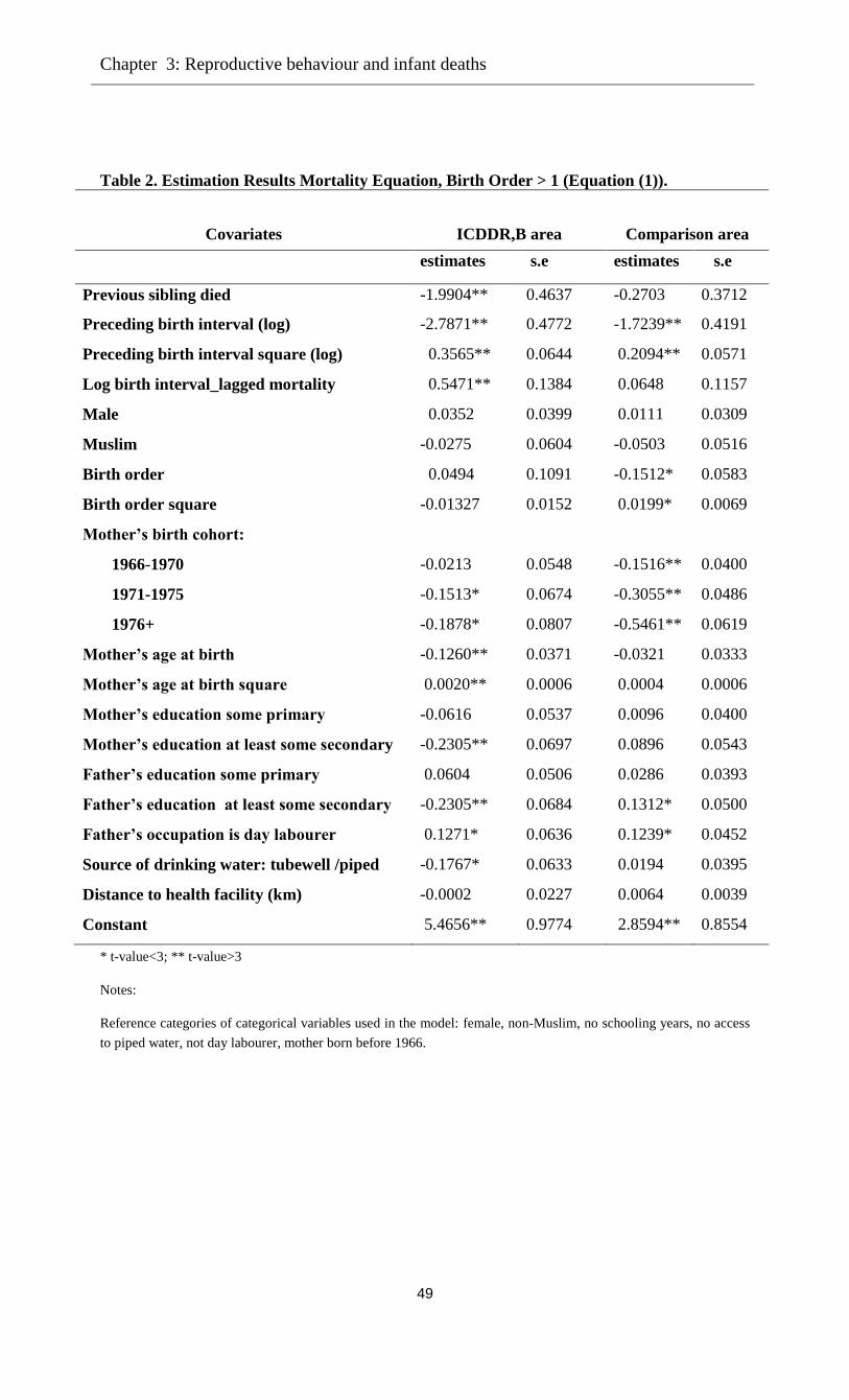
Chapter 3: Reproductive behaviour and infant deaths
49
Table 2. Estimation Results Mortality Equation, Birth Order > 1 (Equation (1)).
Covariates
ICDDR,B area
Comparison area
estimates s.e estimates s.e
Previous sibling died -1.9904** 0.4637 -0.2703 0.3712
Preceding birth interval (log) -2.7871** 0.4772 -1.7239** 0.4191
Preceding birth interval square (log) 0.3565** 0.0644 0.2094** 0.0571
Log birth interval_lagged mortality 0.5471** 0.1384 0.0648 0.1157
Male 0.0352 0.0399 0.0111 0.0309
Muslim -0.0275 0.0604 -0.0503 0.0516
Birth order 0.0494 0.1091 -0.1512* 0.0583
Birth order square -0.01327 0.0152 0.0199* 0.0069
Mother’s birth cohort:
1966-1970 -0.0213 0.0548 -0.1516** 0.0400
1971-1975 -0.1513* 0.0674 -0.3055** 0.0486
1976+ -0.1878* 0.0807 -0.5461** 0.0619
Mother’s age at birth -0.1260** 0.0371 -0.0321 0.0333
Mother’s age at birth square 0.0020** 0.0006 0.0004 0.0006
Mother’s education some primary -0.0616 0.0537 0.0096 0.0400
Mother’s education at least some secondary -0.2305** 0.0697 0.0896 0.0543
Father’s education some primary 0.0604 0.0506 0.0286 0.0393
Father’s education at least some secondary -0.2305** 0.0684 0.1312* 0.0500
Father’s occupation is day labourer 0.1271* 0.0636 0.1239* 0.0452
Source of drinking water: tubewell /piped -0.1767* 0.0633 0.0194 0.0395
Distance to health facility (km) -0.0002 0.0227 0.0064 0.0039
Constant 5.4656** 0.9774 2.8594** 0.8554
* t-value<3; ** t-value>3
Notes:
Reference categories of categorical variables used in the model: female, non-Muslim, no schooling years, no access
to piped water, not day labourer, mother born before 1966.
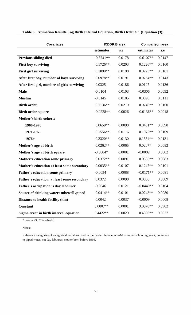
50
Table 3. Estimation Results Log Birth Interval Equation, Birth Order > 1 (Equation (3)).
Covariates
ICDDR,B area
Comparison area
estimates s.e estimates s.e
Previous sibling died -0.6741** 0.0178 -0.6107** 0.0147
First boy surviving 0.1726** 0.0203 0.1226** 0.0160
First girl surviving 0.1099** 0.0198 0.0723** 0.0161
After first boy, number of boys surviving 0.0978** 0.0191 0.0764** 0.0143
After first girl, number of girls surviving 0.0325 0.0186 0.0197 0.0136
Male -0.0104 0.0103 -0.0306 0.0092
Muslim -0.0145 0.0105 0.0090 0.0111
Birth order 0.1136** 0.0219 0.0746** 0.0160
Birth order square -0.0228** 0.0026 -0.0136** 0.0018
Mother’s birth cohort:
1966-1970 0.0659** 0.0098 0.0461** 0.0090
1971-1975 0.1556** 0.0116 0.1072** 0.0109
1976+ 0.2320** 0.0130 0.1554** 0.0131
Mother’s age at birth 0.0262** 0.0065 0.0207* 0.0082
Mother’s age at birth square -0.0004* 0.0001 -0.0002 0.0002
Mother’s education some primary 0.0372** 0.0091 0.0565** 0.0083
Mother’s education at least some secondary 0.0035** 0.0107 0.1247** 0.0101
Father’s education some primary -0.0054 0.0088 -0.0171** 0.0081
Father’s education at least some secondary 0.0372 0.0098 0.0066 0.0089
Father’s occupation is day labourer -0.0046 0.0121 -0.0440** 0.0104
Source of drinking water: tubewell /piped 0.0414** 0.0101 0.0243** 0.0080
Distance to health facility (km) 0.0042 0.0037 -0.0009 0.0008
Constant 3.0807** 0.0801 3.0370** 0.0982
Sigma error in birth interval equation 0.4422** 0.0029 0.4356** 0.0027
* t-value<3; ** t-value>3
Notes:
Reference categories of categorical variables used in the model: female, non-Muslim, no schooling years, no access
to piped water, not day labourer, mother born before 1966.
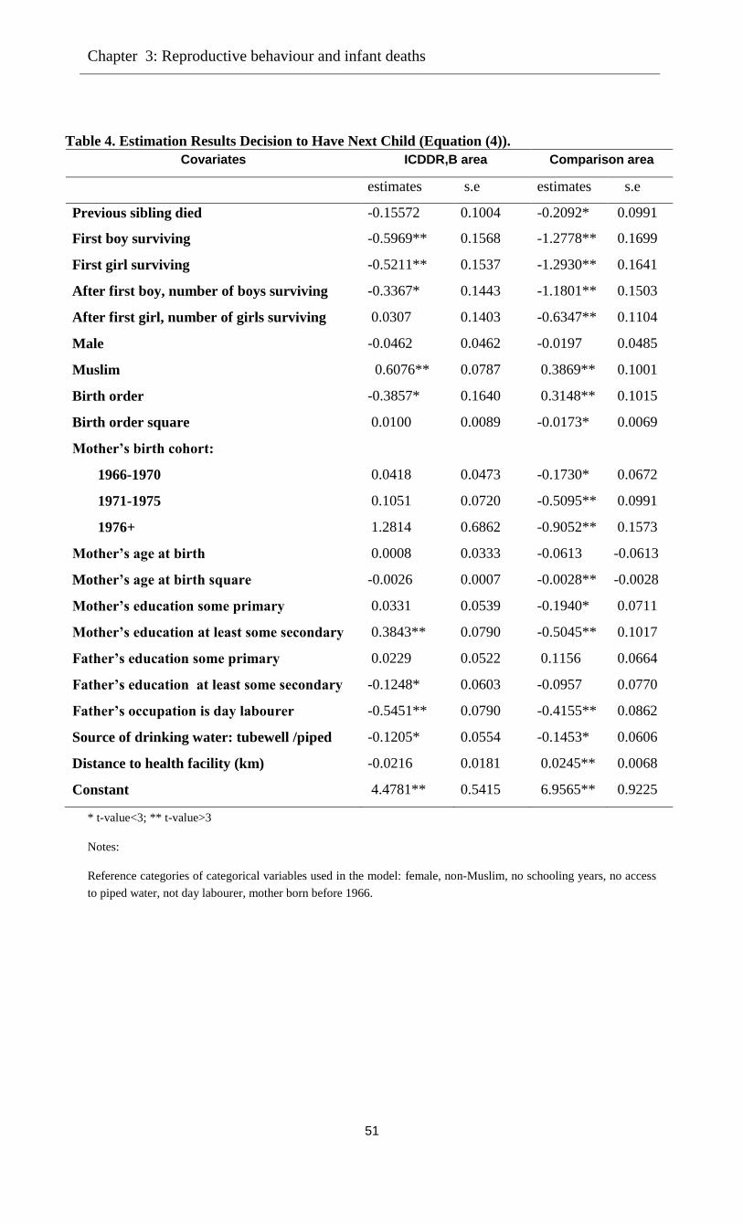
Chapter 3: Reproductive behaviour and infant deaths
51
Table 4. Estimation Results Decision to Have Next Child (Equation (4)).
Covariates ICDDR,B area Comparison area
estimates s.e estimates s.e
Previous sibling died -0.15572 0.1004 -0.2092* 0.0991
First boy surviving -0.5969** 0.1568 -1.2778** 0.1699
First girl surviving -0.5211** 0.1537 -1.2930** 0.1641
After first boy, number of boys surviving -0.3367* 0.1443 -1.1801** 0.1503
After first girl, number of girls surviving 0.0307 0.1403 -0.6347** 0.1104
Male -0.0462 0.0462 -0.0197 0.0485
Muslim 0.6076** 0.0787 0.3869** 0.1001
Birth order -0.3857* 0.1640 0.3148** 0.1015
Birth order square 0.0100 0.0089 -0.0173* 0.0069
Mother’s birth cohort:
1966-1970 0.0418 0.0473 -0.1730* 0.0672
1971-1975 0.1051 0.0720 -0.5095** 0.0991
1976+ 1.2814 0.6862 -0.9052** 0.1573
Mother’s age at birth 0.0008 0.0333 -0.0613 -0.0613
Mother’s age at birth square -0.0026 0.0007 -0.0028** -0.0028
Mother’s education some primary 0.0331 0.0539 -0.1940* 0.0711
Mother’s education at least some secondary 0.3843** 0.0790 -0.5045** 0.1017
Father’s education some primary 0.0229 0.0522 0.1156 0.0664
Father’s education at least some secondary -0.1248* 0.0603 -0.0957 0.0770
Father’s occupation is day labourer -0.5451** 0.0790 -0.4155** 0.0862
Source of drinking water: tubewell /piped -0.1205* 0.0554 -0.1453* 0.0606
Distance to health facility (km) -0.0216 0.0181 0.0245** 0.0068
Constant 4.4781** 0.5415 6.9565** 0.9225
* t-value<3; ** t-value>3
Notes:
Reference categories of categorical variables used in the model: female, non-Muslim, no schooling years, no access
to piped water, not day labourer, mother born before 1966.

52
Table 5. Mother specific unobserved heterogeneity.
Mortality Birth interval Fertility
ICDDR,B area
Covariance matrix
Mortality 0.301**
Birth interval -0.012 0.017**
Fertility 0.189 -0.099** 0.793**
Correlation matrix
Mortality 1
Birth interval -0.167 1
Fertility 0.386 -0.856** 1
Comparison area
Covariance matrix
Mortality 0.063**
Birth interval -0.0002 0.007**
Fertility -0.188** -0.088** 2.306**
Correlation matrix
Mortality 1
Birth interval -0.012 1
Fertility -0.495** -0.698** 1 ** t-value>3
Table 6. Simulations.
ICDDR,B area 1 2 3 4 5
Infant mortality 51.8/1000 -0.27 4.85 -2.26 1.63
Median birth interval
(months)
43.12 5.87 -0.20 0.70 3.87
Number of births (fertility) 2.43 -2.20 0.01 -0.20 -3.32
Number of survivors 2.31 -2.18 -0.26 -0.08 -3.40
Comparison area
Infant mortality 68.5/1000 -3.57 1.560 2.208 0.43
Birth interval (months) 35.95 6.30 -0.20 -0.10 3.15
Number of births (fertility) 2.75 -3.72 -0.35 0.73 -5.68
Number of survivors 2.56 -3.47 -0.46 0.57 -5.71
Notes: Column 1 presents simulated outcomes for the benchmark model. Columns 2-5 show percentage deviations
from the benchmark outcomes that arise when selected mechanisms are “switched off” as follows:
Column 2: no effect of infant mortality on birth interval or probability of having another child
Column 3: no direct effect of lagged mortality on mortality
Column 4: no correlation between unobserved heterogeneity in mortality equation and other equations (no hoarding)
Column 5: birth spacing and family planning as if all children are boys (no gender preference in birth intervals or
probability of having another child)
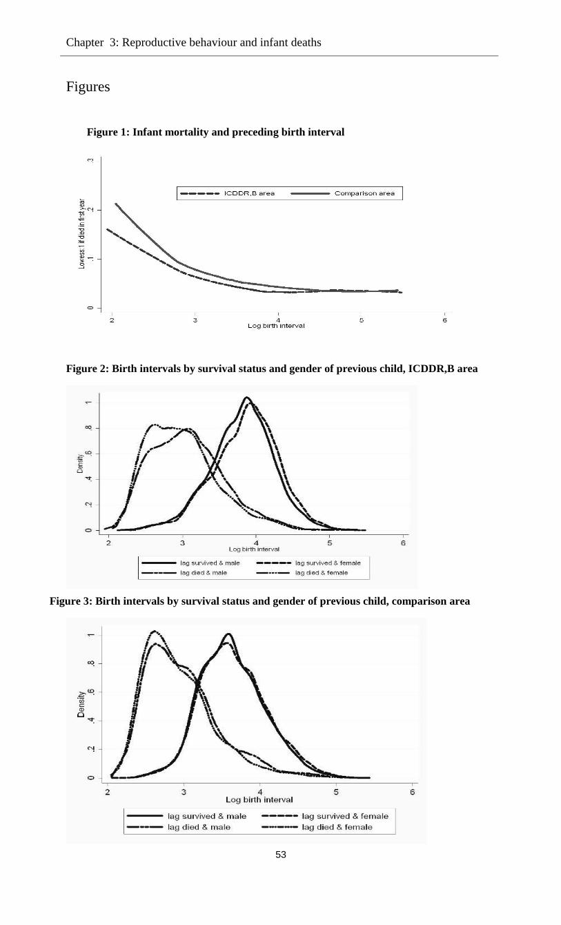
Chapter 3: Reproductive behaviour and infant deaths
53
Figures
Figure 1: Infant mortality and preceding birth interval
Figure 2: Birth intervals by survival status and gender of previous child, ICDDR,B area
Figure 3: Birth intervals by survival status and gender of previous child, comparison area
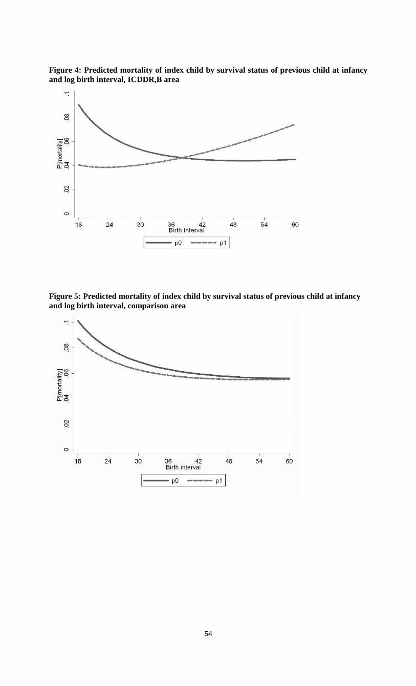
54
Figure 4: Predicted mortality of index child by survival status of previous child at infancy
and log birth interval, ICDDR,B area
Figure 5: Predicted mortality of index child by survival status of previous child at infancy
and log birth interval, comparison area

Chapter 4
Does Family Planning Reduce Infant Mortality?
Evidence from Surveillance Data in Matlab,
Bangladesh11
4.1 Introduction
Family planning programs were initiated for the wellbeing of mother and child. The mechanisms
involved relate to family-building patterns like short birth intervals, young (or relatively old) age
of the mother at birth, and many births in a short time period. Births that occur at the extremes of
maternal age or are preceded by very short birth intervals are at higher mortality risk, as is
widely discussed in the demographic literature (see for example, Haaga 1989; Alam and David
1998; Arulampalam and Bhalotra 2006; Omariba et al. 2008; DaVanzo et al. 2008). Through
family planning practice a couple can decide the time of birth, the time span between two births,
and the (maximum) number of children they want to have. Contraceptive use is a means of
family planning and if it leads to a reduction in the proportion of births at these high risks then
infant mortality in the population would decline if the level of contraceptive use rises.
Several studies conducted in Bangladesh (and the Matlab region in particular) reveal that
the percentage of lower–order births has increased with rising contraceptive use (for example,
Koenig et al. 1992; LeGrand and Phillips 1996). By reducing the number of infants born,
contraceptive use can enhance the chances for survival: It can, for example, avoid contamination
of infectious diseases among closely spaced siblings or reduce siblings’ competition for scarce
resources such as parental time allocated to child care or the availability of food. Potter (1988)
emphasized that proportionally greater reduction of fertility among women whose reproductive
health status is poor and the change in family relationships and parenting practices may be
crucial ways in which family planning can favourably affect infant mortality.
However, while the theoretical acceptance is wide, empirical evidence on the conjecture
that family planning reduces infant mortality is rare. The magnitude of such an effect is also in
question. Demographers have different views about the favourable effects of family planning on
infant mortality and this thus remains an important issue for further investigation (for reviews see
Bongaarts 1987; Trussell 1988; Potter 1988; LeGrand and Phillips 1996). Different explanations
11
This chapter is joint work with Arthur van Soest, Tilburg University. This paper has been presented in the
international conference Population Association of America (PAA) 2011, Washington, D.C, USA. We thank the
conference participants and members of committee for their helpful comments and suggestions.
56
are documented in the literature. Bongaarts argues that the direct effects of contraceptive use on
mother’s age at birth, birth interval and the number of higher order births are largely offset by the
rise in the proportion of high-risk first births, so that the net effect of contraceptive use on infant
mortality is small. Secondly, he argues that many of the apparent effects of child-bearing patterns
on child mortality are correlated with other factors (see Hobcraft et al. 1985), which needs to be
taken into account in the analysis. Several researchers disagree with Bongaarts’s first argument.
For example, Trussell (1988) argues that Bongaart’s analysis is likely to mislead policy makers
because the fraction of first births automatically rises due to the total fertility decline, so that the
total infant mortality rate at aggregate level is a misleading measure of child health. He
emphasizes the need of taking into account the artificial inflation of first-borns when measuring
the impact of family planning on infant mortality at the aggregate level. He also argues that the
mortality reducing effect of family planning is important among women who use contraception
to space their births or to eliminate unwanted high order births.
A recent review conducted by Yeakey et al. (2009) emphasizes the policy relevance of
studying the behavioural pathways linking contraceptive use to birth spacing and timing of births
and to perinatal and infant mortality. They reviewed fourteen studies, which all find that the use
of contraceptives is protective against short birth intervals. This review also points out
methodological flaws of the existing studies, which could undermine the accepted rationale for
expanding family planning programs to help deliver the maternal and child health benefits of
birth spacing. Existing studies typically use retrospective birth-history data collected in cross-
sectional surveys, potentially introducing recall bias and heaping of birth intervals at six-month
intervals. A few studies investigated either ever-use or never-use of contraceptives by mothers,
not considering the timing of contraceptive use in relation to births.
According to this review none of the existing studies used randomized controlled trials to
test the effect of contraceptive use on the outcome of interest-infant mortality. Implementing
such a design would require not only a very large sample size, but also monitoring continuous
episodes of contraceptive use, pregnancies, conceptions, completion of pregnancies, and the
morbidity and mortality outcomes of mother and child at least one year postpartum. Indeed, in
this regard it seems that an observational design is perhaps inevitable as a feasible alternative.
Ideally such a design should be implemented prospectively. Thus, the use of the prospective data
from Matlab Bangladesh might be a good alternative for randomized controlled trials (see for
example Phillips et al. 1982). Several studies using Matlab data investigated the determinants of
infant mortality (DaVanzo and Starbird 1991; Hale et al. 2006; DaVanzo et al. 2007, 2008).
However, these studies do not assess explicitly the magnitude of the effect of contraceptive use.
Taking into account limitations of all fourteen studies, and in line with the emphasized
importance of taking into account correlation and unobserved heterogeneity (Hobcraft et al. 1985;
LeGrand and Phillips 1996), the review of Yeakey et al. (2009) concludes that more rigorous
modelling is needed, preferably on the basis of longitudinal prospective data. This is exactly
where the current study aims to contribute.
Chapter 4: Family planning practice and infant deaths
57
In the Matlab ICDDR,B area community health workers through their monthly routine
visits record episodes of contraceptive use, pregnancies, conceptions, and the morbidity and
mortality outcomes for all children until five years old. Therefore, using longitudinal prospective
data from Matlab known to be of exceptional accuracy and completeness, this study first
investigates the effects of infant death and other factors (such as socio-economic status or gender
composition of the household) on subsequent contraceptive use, and second, the effects of
contraceptive use after a birth on birth intervals and infant mortality. Our main analysis is based
upon a model with three parts: an equation explaining infant mortality, a model part that explains
whether contraceptives are used after a child is born, and an equation explaining birth intervals.
(Sterilization is not considered since the mothers in our sample did not initiate sterilization.)
Infant mortality is determined by covariates reflecting socio-economic status, age of the mother,
gender of the child, etc., but also by the length of the preceding birth interval. The decision to use
contraceptives is driven by similar covariates, but also by survival status of the previous child
and the family’s gender composition. Birth spacing is driven by contraceptive use and other
factors.
Each part of the model also incorporates unobserved mother specific heterogeneity, and
the various unobserved heterogeneity terms are allowed to be correlated, so that the estimates of
the parameters reflecting the causal effects are consistent under general assumptions about the
nature of heterogeneity. This makes the model similar in spirit to a recently developed model for
birth spacing, fertility, and neonatal mortality in Bhalotra and van Soest (2008). Furthermore, we
perform simulations aimed at uncovering the linkage between contraceptive use, birth spacing
and infant mortality, taking into account the effect of an increasing fraction of first- born children
on the aggregate infant mortality rate.
4.2 Data
4.2.1 ICDDR,B area and interventions
The International Centre for Diarrheal Disease Research, Bangladesh (ICDDR,B) started the
Maternal Child Health and Family Planning (MCH-FP) programme in October 1977 in half of
the health and demographic surveillance system (HDSS) area in Matlab to assess the extent to
which maternal and child health and family planning services can reduce fertility and mortality
in a rural population. In this area, formerly known as MCH-FP area and currently as ICDDR,B
area, additional health services were provided and data were collected on events like births,
deaths, causes of deaths, marriage, divorce, migration-in, migration-out, family planning practice,
and a range of health indicators, for a population of 89,350 from 70 villages. The other half of
the Matlab area remained under the standard government health systems and is known as
comparison area, with a population of 85,596 from 79 villages. The large population of the
ICDDR,B area with different levels of intensity and coverage and the relative isolation of
villages permitted the designation of four treatment blocks where special services are offered,
and of contiguous comparison areas in which demographic dynamics are monitored but the

58
contraceptive-use history data are absent. The data from the comparison area therefore cannot be
used for the purpose of analysis in this paper.
Data have been collected systematically through regular household visits (once every two
weeks until January 1998, and once every month since then). These data, in combination with
ICDDR,B population censuses and surveys, permit the evaluation of health and family planning
services with a degree of accuracy that is rare in low-income settings (LeGrand and Phillips
1996). Analysis of levels and trends and a comparison between the ICDDR,B area and the
comparison area shows clear evidence that the MCH-FP intervention reduces fertility and under-
five mortality (see for example, LeGrand and Phillips 1996; Hale et al. 2006; DaVanzo et al.
2007, 2008).
4.2.2 Study sample
We analyse a sample of 31,968 singleton live births and 13,232 mothers who
continuously lived and gave all their births in the ICDDR,B area. The data cover the period July
1982 to December 2005; the data before 1982 are not (yet) available for this type of research. A
similar set of data was used in several companion papers like Saha and van Soest (2011), but this
is the first time we also consider the contraceptive use data available after each birth.
4.2.3 Variables and descriptive statistics
The dependent variables in our models are the length of each time interval between births,
a dummy for using contraceptives after each birth, and a dummy for infant mortality of each
child born alive. The covariates include birth order of the child, gender of the child, and age of
the mother at the time of birth of the child; education of the mother is captured by dummy
variables; this may proxy the mother’s ability to take good care of her children but may also
proxy the family’s socio-economic status. Education and occupation of the father also reflect the
family’s socio-economic status. Another family level covariate is religion, which is included
because contraceptive practice may vary between the two groups. In Matlab, different patterns of
fertility behaviour are observed by religion (Huffman et al. 1987). To control for environmental
factors, we include a dummy for access to running drinking water (a dummy for piped drinking
water / tube well), and the distance to the nearest health facility (defined as a sub-centre or
ICDDR,B hospital).
The average number of children born per mother is 2.42 and 82.7 percent of all mothers
in the sample are Muslims. The mean age of mothers at birth is respectively 24.7 years, and the
average birth interval is about 48 months with standard deviation 23 months, and about 11
percent birth intervals are shorter than 24 months. 48 percent of all mothers never attended
school. On average, mothers residing within 2 kilometres of distance to a health facility and 88
percent of all mothers have access to running water (tube well/pipe water).
During the observation period (July 1982-December, 2005), mothers used contraceptives
after about 84 percent of all 31,968 child births. In 11 percent of all cases they did not use

Chapter 4: Family planning practice and infant deaths
59
contraceptives, and about in 4.8 percent of all cases the information on contraceptive use was
missing (see Figure 1). The missing observations occur for the most recent births because it is
too early to observe contraceptive use status. The average duration of contraceptive use is about
31.4 months with a standard deviation 27.9 months. In about 12 percent of all cases, mothers
started using contraceptives more than one year after the previous birth (see Figure 1). In about
55 percent of all cases, they started using contraceptives earlier than 12 months after the previous
birth and continued until more than 12 months after birth (see Figure 1). These are the cases
where mothers were using contraceptives exactly one year after their previous birth.
Among users, 20.67 percent used pills, 46.63 percent used injections, 4.74 percent used
IUD, 11.06 percent used condoms, 0.43 percent used sterilization and 0.81 percent used a
traditional method.
Table 1 shows that there is a clear positive relationship between contraceptive use and
birth interval length. The birth interval until a next birth is about 53 percentage points (from 24
percent to 77 percent) more likely to be longer than 36 months if a mother uses contraceptives at
any time after birth (irrespective of starting time and continuation). There is some variation
between the birth interval and the contraceptive method used: using injections or condoms is
associated with longer birth intervals than using other methods (pill, traditional, IUD; not shown
in the Table).
The bivariate relationships between the socioeconomic variables and contraceptive use
and infant mortality are given in Table 2. The results are in line with expectations; for example,
first births, shorter preceding time intervals between births, mothers younger than 20, and
illiterate mothers are particularly disadvantaged in terms of child survival, and also in
contraceptive use. For most covariates, the association with child mortality is opposite to that
with using contraceptives, but there are some exceptions. For example, although contraception is
higher among Hindu than among Muslim families, it is evident that infant mortality is also
higher among Hindus. The latter is in line with findings for India; see Bhalotra et al. (2010a,b).
Finally, Table A1 in the annex gives a more detailed picture of the associations between
contraceptive use and infant mortality of successive children. First, it shows that contraceptive
use after a given birth is much less common when the child that is born dies during its infancy
than when it survives its infancy (the contraceptive use rates are 46.4% (=617/1331*100%) and
83.4%, respectively. Second, the infant mortality rate among children born after an interval
during which contraceptives have been used is much smaller than the infant mortality rate among
births not preceded by contraceptive use (34.0 versus 62.2 per 1000 births). A possible
explanation may be that contraceptive use helps to avoid short birth intervals and short intervals
lead to larger mortality risk, but alternative explanations are possible, such as common observed
or unobserved factors driving mortality and family planning decisions. The econometric model
will disentangle these various explanations.

60
4.3 Model
The model explains infant mortality (that is, whether the child survives its first twelve months or
not) of each child born, contraception decisions after each live birth, intervals between live
births, and fertility decisions. It builds on the model of Bhalotra and van Soest (2008) but adds
the decisions to use contraceptives or not. To be precise, the endogenous variables in the model
are the following, with i denoting a mother and t=1,..,Ti denoting consecutive live births:
itM : Infant mortality dummy: 1 if child t dies; 0 if it survives the first twelve months after birth.
itC : Contraceptive use dummy: 1 if mother i uses contraception after giving birth to child t; 0
otherwise.
itF : Decision to have another child (1) or not (0).
itB : Log birth interval preceding birth of child t (t>1 only)
The sequence of events, which is the basis for the dynamic structure of the model, is illustrated
in the following time line:
1 1,i iC F 2 2,i iC F 3 3,i iC F 4 4,i iC F
---+--------------+--------------+----------------+----- 1iM 2iB 2iM 3iB 3iM 4iB 4iM
We do not explain the timing of the first birth (or the decision to use contraceptives
before the first birth. The first event we explain is infant survival of the first born child 1iM . The
second is the decision to use contraceptives or not at any time after birth 1 and (if there is a
second birth) before birth 2 ( 1iC ). The information on the exact timing of contraceptive use
(starting and ending date) is not very reliable, which is why we only explain the binary decision.
Since contraception usually starts at least one year after a live birth, it is a good approximation to
treat this variable as an event that takes place when infant mortality of the latest born child is
already known. At the same time, the mother also may decide not to have any more children
( 1iF ); this decision is never observed directly, but if a next birth is observed we know that 1 1iF .
If 1 1iF , a next birth will take place, and if it takes place before the end of the survey
window, we observe the birth interval 2iB . The second born child can die during infancy or
survive, etc.: the sequence of events continues until the mother decides not to have more children
( 0iTF ) or at the end of the observation period (December 2005).
The model we use is recursive in the sense that each dependent variable may depend on
outcomes realized earlier in the sequence of events, but not on future outcomes. Moreover, each
outcome may depend on unobserved factors common to all children of a given mother, treated as
unobserved individual effects. We use probit equations for the binary outcomes and a regression

Chapter 4: Family planning practice and infant deaths
61
equation for the continuous outcomes. Below we discuss the equations for the various outcomes
in detail.
Infant mortality
The equation for infant mortality is similar to that in Bhalotra and van Soest (2008). For
higher birth orders, a dynamic probit equation with random mother specific effects is used,
where the regressors include the preceding birth intervals and variables like the mother’s age at
birth, which is a function of previous birth intervals: For child t (t=2,…,Ti) of mother i, the
equation is
Mit* =Xit βm + Zitγm + mi + umit (1)
Mit=1 if Mit*>0 and Mit=0 if Mit
*≤0
Here itX contains (functions of) the strictly exogenous variables, such as gender of the child,
socio-economic status indicators of the household (mother’s and father’s education, etc.) and
characteristics of the village where the household resides. Zit denotes the vector of explanatory
variables that are functions of previous outcomes (and are therefore not strictly exogenous). It
includes the preceding log birth interval Bit, but also (functions of) age of the mother at birth t
and, following the literature on scarring (see, for example, Arulampalam and Bhalotra 2006),
survival status of the previous child Mit-1. The mother specific unobserved heterogeneity term
mi captures unobservable time invariant characteristics influencing the propensity do die of all
children in the family. The error term umit captures idiosyncratic health shocks specific to child t.
We assume that the mitu follow a standard normal distribution, independent of each other and of
all covariates, and that mi is normally distributed with mean 0 and variance 2
m independent of
all umit and itX (but not of Zit).
For mortality of the first child, a separate equation is needed, since in this case there is no
preceding birth interval and no preceding mortality outcome. Age at first birth is assumed to be
strictly exogenous and can therefore be included in 1iX . The equation for infant mortality of child
1 is then given by:
Mi1* =Xi1 β
1 + θmi + umi1 (2)
Mi1=1 if Mi1*>0 and Mi1=0 if Mi1
*≤0
Here β1 and θ are additional parameters to be estimated and the error term umi1 is assumed to
satisfy the same assumptions as the other umit .
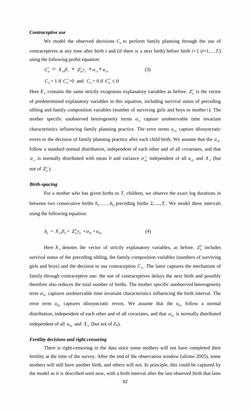
62
Contraceptive use
We model the observed decisions itC to perform family planning through the use of
contraceptives at any time after birth t and (if there is a next birth) before birth t+1 (t=1,…,Ti)
using the following probit equation:
*
itC = citX + c
it cZ + ci + citu (3)
itC = 1 if *
itC >0 and itC = 0 if 0* itC
Here itX contains the same strictly exogenous explanatory variables as before. c
itZ is the vector
of predetermined explanatory variables in this equation, including survival status of preceding
sibling and family composition variables (number of surviving girls and boys to mother i ). The
mother specific unobserved heterogeneity terms ci capture unobservable time invariant
characteristics influencing family planning practice. The error terms citu capture idiosyncratic
errors to the decision of family planning practice after each child birth. We assume that the citu
follow a standard normal distribution, independent of each other and of all covariates, and that
ci is normally distributed with mean 0 and variance 2
c independent of all citu and itX (but
not of c
itZ ).
Birth-spacing
For a mother who has given births to iT children, we observe the exact log durations in
between two consecutive births 2ib ,….,iT ib preceding births 2,....., iT . We model these intervals
using the following equation:
itb = bitX + b
it bZ + bi + bitu (4)
Here itX denotes the vector of strictly explanatory variables, as before. b
itZ includes
survival status of the preceding sibling, the family composition variables (numbers of surviving
girls and boys) and the decision to use contraception itC . The latter captures the mechanism of
family through contraceptive use: the use of contraceptives delays the next birth and possibly
therefore also reduces the total number of births. The mother specific unobserved heterogeneity
term bi captures unobservable time invariant characteristics influencing the birth interval. The
error term bitu captures idiosyncratic errors. We assume that the bitu follow a normal
distribution, independent of each other and of all covariates, and that bi is normally distributed
independent of all bitu and itX (but not of Zit).
Fertility decisions and right censoring
There is right-censoring in the data since some mothers will not have completed their
fertility at the time of the survey. After the end of the observation window (ultimo 2005), some
mothers will still have another birth, and others will not. In principle, this could be captured by
the model as it is described until now, with a birth interval after the last observed birth that lasts

Chapter 4: Family planning practice and infant deaths
63
longer than till the end of 2005. Following Bhalotra and van Soest (2008), however, the model fit
can be improved substantially by adding a separate equation reflecting the possible decisions to
stop having children after each birth. The reason why this improves the fit is essentially that it
can explain why some mothers who are still of reproductive age have no more births long before
the end of the observation window. (We will assume that women are no longer of reproductive
age when they reach age 45, an age beyond which very few births are observed in our data).
Without the additional equation, this would have to be explained by a very long birth interval.
The equation determining whether the woman continues to have children after birth t
(Fit=1) or not (Fit=0) is specified as follows:
*
itF = fitX +
f
it fZ +fi +
fitu (5)
itF = 1 if *
itF >0 and itF = 0 if 0* itF
As before, itX denotes the vector of strictly exogenous explanatory variables. The vector f
itZ
includes survival status of the preceding sibling and family composition variables (based upon
the number of surviving girls and boys). The mother specific unobserved heterogeneity term fi
captures unobservable time invariant characteristics influencing the fertility decision after each
child birth. The term fitu captures idiosyncratic errors. We assume that the errors
fitu are standard
normally distributed, independent of each other and of all covariates. The mother specific
unobserved heterogeneity terms fi are normally distributed with mean 0 and variance
2
f ,
independent of all fitu and itX .
The outcome itF is observed only partially. If birth t is not the last birth (t<Ti) then we
know that the mother has decided not to stop having children, so itF = 1. But if t=Ti, it is possible
that she has decided to stop having children ( itF = 0), but it may also be the case that the next
birth interval extends beyond the end of the observation window ( itF = 1 and right censoring).
Note that we have neither included contraceptive use as an explanatory variable for the
decision to continue fertility, nor the fertility choice as a factor driving contraceptive use. This is
because we see these two decisions as taken jointly (and at the same point in time), as illustrated
on the time line at the beginning of this section. It is clear that the two decisions are related but
modelling the mechanics of the decision process is beyond the scope of this study. Instead, we
model two decisions in a reduced form type of way, not including the other decision on the right
hand side.12
Confounding unobserved factors are controlled for by allowing arbitrary correlations
amongst fi, mi, bi, and ci. We will assume they are drawn from a four-dimensional normal
distribution with zero mean and an arbitrary covariance matrix, independent of the itX and all the
idiosyncratic error terms.
12
One might argue that this implies that the error terms in equations (5) and (3) should be correlated. This is an
extension we leave for future work.
64
The five equations of this model (including the initial mortality equation) are estimated
jointly using simulated maximum likelihood. Conditional on the random mother specific effects,
the likelihood contribution of a given mother can be written as a product of univariate normal
probabilities and densities over all births following the order of observed events as indicated on
the time line sketched above and accounting for the possibility of right censoring. Since mother
specific effects are unobserved, the actual likelihood contribution is the expected value of the
conditional likelihood contribution, with the expected value taken over the four random effects.
This is a four-dimensional integral, which is approximated using (smooth) simulated ML:
Multivariate errors drawn from N(0,I4) are transformed into draws of the random effects using
the parameters of the random effects distribution; the conditional likelihood contribution is then
computed for each draw and the mean across R independent draws is taken. If R with the
number of mothers N, this gives a consistent estimator; if draws are independent across
households and R faster than N, then the estimator is asymptotically equivalent to exact ML
(see, for example, Hajivassiliou and Ruud 1994). To reduce the sampling variance in the
simulations, we used Halton draws (see Train 2003). The results we present are based on R=50.
We checked the sensitivity of our parameter estimates for the number of the draws (comparing
with larger R) and the nature of the draws (using Halton draws with different seeds) and always
got very similar results, as in chapter 3. The estimation procedure is very similar in spirit to the
one used by Bhalotra and van Soest (2008); see also their online appendix for details.
4.4 Estimation results
Table 3 reports the parameter estimates, using the benchmark definition of contraceptive use.
The estimates of the specification with an alternative definition of the contraceptive use dummy
are presented in Table A2 in the appendix. In the discussion in this section we focus on the
benchmark specification; the results in Table A2 will be discussed in Section 6. The top panel of
the Table presents the estimates of the parameters in the four main equations; the bottom panel
shows the estimates of the covariance structure of the unobserved heterogeneity terms. Estimates
for the static equation for mortality of the first child are available upon request; they are very
similar to those in Saha and van Soest (2011).
Contraceptive use
The estimates in the contraceptive use equation are in line with existing results on the
determinants of contraceptive use in rural Bangladesh; see for example, Koenig et al. (1992) or
Rahman et al. (1992). Acceptance of contraception is significantly (at the 5 percent level) higher
among Hindus than among Muslims, in line with the bivariate relation in Table 2. The estimated
difference in the probability to use contraceptives keeping other observed and unobserved
characteristics constant is about 1.7 percentage points.13
Contraceptive use is increasing in both
maternal and paternal education, with larger effects of paternal education. The strong association
13
Estimated marginal effects (keeping other observed and unobserved characteristics constant) for the average
observation are about 0.19 times the corresponding parameter estimate.

Chapter 4: Family planning practice and infant deaths
65
with parental education levels is in line with Rahman et al. (1992, Table 1), while Koenig et al.
(1992, Table 3) find a much weaker relation with maternal education in the ICDDR,B area. If the
father is a day-labourer, however, contraceptive use is significantly more likely, which is not in
line with the bivariate relationship in Table 2. Perhaps these families have a larger tendency to
postpone having more children until the socio-economic position of the breadwinner improves.
The likelihood of contraceptive use is increasing in the mother’s age at birth, a common pattern
in developing country data. Mothers of later birth cohorts exhibit a significantly increasing trend
of contraceptive use.
The death of the last born child at infancy substantially reduces the likelihood of
contraceptive use (by about 17 percentage points in the benchmark specification), in line with the
replacement hypothesis that families want to replace a lost child. This is widely regarded in the
demographic literature (for example, see Rahman et al. 1992 or Bhalotra and van Soest 2008).
The effects of the numbers of surviving boys and girls are consistent with son preference: having
at least one boy has a somewhat stronger (positive) effect on the decision to use contraceptives
than having at least one girl (the marginal effects are about 10.0 and 8.4 percentage points), and
each additional son in the family increases the likelihood of contraceptive use more than each
additional daughter (with, for the average observation, about 6.7 and 3.4 percentage points,
respectively). Similar conclusions concerning son preference in family planning have been
drawn in other studies for Bangladesh (see for example, Rahman et al. 1992; Koenig et al. 1992).
Birth intervals
The parameter estimates in the log birth-spacing equation show that, keeping constant
other factors including the decision to use contraceptives at any time after the previous birth,
birth intervals tend to be shorter for high birth orders, which is consistent with the stylized fact
that short birth intervals are associated with high fertility. Mothers with more education
consistently have longer birth intervals. Birth spacing is increasing in maternal age. In more
developed villages with piped/tube well water, birth intervals are longer.
As expected, using contraceptives leads to a large and significant increase in the space
between births – it increases the interval by around 60 percent (exp(0.495)-1)*100%). On the
other hand, keeping contraceptive use and other factors constant, death at infancy of the previous
child shortens the subsequent interval between births by 43 percent (exp(-0.55)-1)*100%), in line
with the replacement hypothesis. The effects of the surviving numbers of boys and girls are again
consistent with son preference: having a boy increases the birth interval by twice as much as
having a girl, and each additional boy has a much larger effect than each additional girl. These
findings are consistent with the earlier findings in the contraceptive equation. These results show
that the decision to use contraceptives and the length of the birth interval conditional on the
decision to use contraceptives (which will depend upon starting and ending date of contraceptive
use, which are not explicitly modelled) are both determined by similar family planning
considerations.

66
Infant mortality
The parameter estimates in the mortality equation in Table 3 are largely in line with the
general conclusions about the determinants of infant mortality in developing countries (see
Bhalotra and van Soest 2008; Omariba et al. 2008) and our findings in chapter 2 or in Saha and
van Soest (2011). A difference compared to our earlier study (chapter 2) is that we find that the
effect of lagged mortality on the probability of infant death of the index child is negative but
insignificant, where in chapter 2(Table 5) this effect was negative and significant at the 5 percent
level when the birth interval was controlled for as an exogenous covariate. This small and
insignificant parameter estimate suggests that a negative learning effect is compensated by a
positive scarring effect through, for example, depression induced by the previous infant’s death.
We allow for a nonlinear relation between birth intervals and infant mortality. The estimates
imply that mortality risk falls with the length of the birth interval over most of the relevant range
of birth intervals (until about 57 months), a finding which is in line with the existing literature
(see, for example, Rutstein, 2005, or Conde-Agudelo et al., 2006). Taking account of the
nonlinear relation between birth spacing and infant death, we find that at the average birth
interval length, an increase of the birth interval by 10 percent reduces mortality by about 0.11%-
points. Since the effect of contraceptive use on the log birth interval is about 0.495, this implies
that, for the average observation, using contraceptives reduces the mortality probability by about
5.4 deaths per 1000 live births.
Fertility
The final column of Table 3 presents the estimates of the auxiliary fertility equation
explaining whether, after each birth and mortality outcome, a family decides to have another
birth or not. Fertility falls with the level of education of both mother and father, with mother’s
education having the larger effect. Muslims show a higher tendency to continue fertility than
their Hindu counterparts, and this finding is consistent with contraception differentials by
religion. It is less clear why, keeping other factors constant, the probability to have another birth
is highest among the youngest birth cohort of mothers and increases with the mother’s age at
previous birth. In villages with access to running water (tube well or piped water) mothers are
less likely to continue their fertility. The family composition variables again show evidence of
son preference in family planning, consistent with the findings in both the contraceptive use and
the birth spacing equation.
Unobserved heterogeneity
The bottom panel of Table 3 describes the estimated covariance structure of the
unobserved heterogeneity terms. (The covariance matrix is specified as ΛΛ’ for a positive semi-
definite lower triangular matrix Λ; the estimated auxiliary parameters are not presented to save
space) Unobserved mother specific heterogeneity is large and significant in the contraceptive and
fertility equations, reflecting 33 percent and 44 percent (denoted in the table by ρ), of the total
unsystematic variation (for given values of the observed covariates and endogenous explanatory
variables in each equation), compared to only 7 percent in the mortality and birth interval
equations.
Chapter 4: Family planning practice and infant deaths
67
We find a large negative correlation between the unobserved heterogeneity terms in the
fertility and contraceptive use equations, and between the fertility and birth spacing equations.
This suggests that, keeping observed factors constant, mothers who desire more children are less
likely to use contraceptives (corr ),( cifi = -0.73), and anticipate this by reducing birth-spacing
(corr ),( fibi = -0.76). This is consistent with target fertility models discussed in, for example,
Wolpin (1997). The negative correlation of the unobserved heterogeneity terms in the mortality
and contraceptive equations (-0.31) suggests that mothers whose children have relatively high
mortality risks respond to this by planning more children and not using contraceptives. This
interpretation contradicts, however, the (modest) positive correlation between unobserved
heterogeneity terms in the mortality and birth spacing equations (+0.21).
4.5 Simulations
To illustrate the importance of family planning for birth spacing, fertility, and infant mortality,
we performed some simulations, in a similar way as the simulations in Bhalotra and van Soest
(2008, Table 3) and as in chapter 3. These simulations show the benefits of family planning
programs that delay second births through lengthening birth intervals and avoid high risk births
in the young birth cohorts of mother. It illustrates the main novelty of our approach – the fact
that our model incorporates various mechanisms that lead to associations between family
planning, birth spacing, fertility, and mortality outcomes, accounting for the effects of
endogeneity in contraceptive use decisions, timing of births (and therefore also age at birth etc.),
birth intervals, and mortality risks.
The simulations use the covariates (including, for example, date of first birth) as observed
for each mother in the actual sample. We then generated, for each mother in the sample,
unobserved heterogeneity terms, error terms, and new outcomes (the dependent variables in our
model) using the estimated parameters of each equation. The outcomes were generated
recursively, using the timing of the events as sketched in Section 4.3. For example, for a given
mother, we take the date of first birth as given and first generate the mortality outcome of the
first child (using equation (2)). Given simulated mortality, we then generated the contraceptive
use decision and the fertility decision after the first birth (equations (3) and (5)). If the fertility
decision is positive, we then generate a birth interval, and update calendar time and age of the
mother at the second birth. Given these variables and the other covariates and the previous
mortality outcome, we then generate the mortality outcome of the second born child, etc. In this
way we generate complete contraceptive use, fertility, and mortality patterns for each mother in
the sample. To reduce simulation variance, this is repeated 25 times for each mother.14
Column 1 summarizes the simulation outcomes according to a benchmark simulation
where all mechanisms at work in the estimated model are active. This simulation reproduces the
14
The simulations take the parameter estimates as given. In principle, it would be possible to compute a standard
error for each simulation outcome by repeating the simulations for other draws of the model parameters from their
estimated (asymptotic) distribution but this would require a substantial computational effort.

68
means in the raw data, showing that the model is able to reproduce these basic features of the
data. This simulation also reproduces the substantial difference between mortality of first born
children (simulated at 67.2 per 1000 live births) and mortality of higher order births (39.6 per
1000 births on average; 40.4, 37.9, 39.0, 42.2 and 46.8 per 1,000 live births for birth orders 2, 3,
4, 5 and 6, respectively).
The other columns present the deviations from the benchmark considering the two
hypothetical extreme cases of contraceptive use: in column 2, everyone is always assumed to use
contraceptives. In column 3, no contraceptives are used at all. The latter is a more dramatic
change compared to the benchmark than the former, since in the benchmark simulation
contraceptives are used in 88.6 percent of all cases.
The simulation in column 2 shows that, according to our model estimates, if
contraceptives were used after each birth, the average birth interval length would increase by
about four months. Since short birth intervals are then more often avoided, it would also reduce
the mortality risk of higher order births. The estimated reductions in mortality of children of birth
order two and higher would be substantial: 7.9 percent for all birth orders of 2 and higher. It is
particularly large for birth order 2 with a reduction of 9.2 percent (3.7 per 1000 live births – from
40.4 to 36.7; these figures are not shown in the table). The longer birth intervals would also
reduce total fertility, by about 2.4 percent. This implies that the weight of first born children in
the total infant mortality rate will increase. Since the infant mortality risk for first born children
is higher than for higher birth orders (and since contraceptives do not affect this mortality rate),
this composition effect tempers the favourable effect of contraceptives on survival chances of
higher order births: the total infant mortality rate still falls compared to the benchmark situation,
but by much less than the mortality rate for higher birth orders.
Results by maternal education level (not shown in the table) show that the benefits of
complete contraceptive use would be particularly large for the lowest socio-economic status
group, mothers without any education. This is because they have the lowest contraceptive use in
the benchmark situation (84.4% compared to 88.6% for the complete sample) but also because
they have shorter birth intervals and the most vulnerable children (their infant mortality rate
among children of birth order 2 and higher is 49.5 per 1000 births in the benchmark situation,
compared to 39.6 per 1000 for the complete sample). If everyone would use contraceptives after
each birth, birth interval lengths in the no education group would increase by 6 months on
average, and infant mortality among higher order births would fall by 8.7% (compared to 7.9%
for the complete sample). Their total infant mortality rate would fall by 3.2% (2.9% for the
whole sample).
The simulation in column 3 indicates that, if contraceptives were never used after any
birth, the average birth interval length would shorten by more than 13 months, and this would
raise the mortality risks in higher order births by 10.6 percent (from 39.6 to 43.8 per 1000 live
births). Particularly for second order births the effect would be large (6.3 per 1000). The shorter
birth intervals lead to an increase of the total fertility rate by 19.3 percent, implying that the

Chapter 4: Family planning practice and infant deaths
69
weight of first born children in the total infant mortality rate will fall. This leads to a negative
composition effect on the total infant mortality rate, that almost completely compensates for the
rise in mortality of higher order births – the total infant mortality rate increases by 1.6 percent
only (from 51.2 to 52.1 per 1000 live births) compared to the benchmark situation.
4.6 Alternative model specification
Table A2 presents the estimation results for the alternative definition of the contraceptives use
dummy – considering whether a mother uses contraceptives at a specific point in time: exactly
12 months after a given birth. Most of the parameter estimates are similar to those in Table 3, but
there are exceptions, particularly, as expected, in the coefficients of the contraceptives equation.
Muslim mothers are much less likely to use contraceptives after exactly one than Hindu mothers
and the difference is now significant at the 5 percent level. Contraceptive use after one year also
increases significantly with birth order. On the other hand, mother’s education plays a much
smaller role than in Table 3. The effect of lagged mortality is still somewhat stronger than in
Table 3, but, unexpectedly, the effects of the family composition variables (surviving boys and
girls) are much smaller and less significant. These variables still have the expected strong and
significant effects on birth intervals and fertility decisions, but not on the decision to use
contraceptives at the chosen specific point in time.
The effect of contraceptive use defined in this alternative way on birth spacing remains
positive and significant, but is much smaller than in Table 3 (0.341 instead of 0.495), suggesting
that contraceptive use after exactly 12 months does not capture the full effect of contraception
decisions on birth spacing; this is the main reason why we prefer the definition of using
contraceptives at any time instead of the alternative.
Table 5 gives the results of the simulations discussed in the previous section for the
estimated model in Table A2, using the alternative dummy on contraceptive use. The benchmark
simulation predicts that contraceptives are used at exactly one year after birth in 58 percent of all
cases. The other outcomes of the benchmark simulation are similar to those in Table 4 and
reproduce the corresponding statistics in the sample.
The simulation in column 2 of Table 5 shows that, according to our alternative model
estimates, if everyone always used contraceptives at one year after each birth, the average birth
interval length would increase by about 7.5 months. The effect seems larger than in Table 5, but
that is because the change from not using to using contraceptives affects many more cases now
(42 percent rather than 12 percent). As a consequence, mortality of children of birth orders two
and higher would fall by 6.9 percent (from 39.4 to 36.7 per 1000 live births). Again, the
reduction is relatively high for second order births (8.2 percent; not shown in the table). The
longer birth intervals would reduce total fertility by about 6.0 percent. This implies that the
weight of first born children in the total infant mortality rate will increase. This composition
effect tempers the favourable effect of contraceptives on survival chances of higher order births

70
if the total infant mortality rate is considered: the total infant mortality rate falls by only 1.5
percent (from 51.0 to 50.3 per 1000 live births) compared to the benchmark situation.
Column 3 of Table 5 gives the simulation results when no one would use contraceptives
one year after birth. The average birth interval length would fall by about 5.7 months. As a
consequence, mortality of children of birth orders two and higher would rise by a modest 1.4
percent (3.8 percent for children of birth order 2, but smaller effects for higher birth orders),
while total fertility would increase by 8.6 percent. This induces a negative composition effect on
total infant mortality including first children since the weight of relatively vulnerable first born
children falls. This composition effect is larger than the direct effect through birth intervals so
that the sum of the two effects is also negative: total infant mortality falls by 1.1 percent
compared to the benchmark situation.
4.7 Discussion and conclusion
Several studies using Matlab data investigated the determinants of infant mortality (DaVanzo
and Starbird 1991; Hale et al. 2006; DaVanzo et al. 2007 and 2008). However, these studies did
not assess explicitly the magnitude of the effect of family planning programs on birth intervals
and thereafter on infant mortality. The major motivation of our current study is the conclusion
drawn by Bongaarts (1987) and a recent review paper by Yeakey et al. (2009). We use the
prospective pregnancy-history data from Matlab, Bangladesh where community health workers
(CHWs) through their monthly routine visit record episodes of contraceptive use, pregnancies,
conceptions, and morbidity and mortality outcomes for mothers and children younger than five.
Exploiting dynamic econometric panel data modelling, our analysis allows for taking into
account endogeneity of birth intervals in the mortality equation, reverse causality of mortality
and fertility (probability of having further birth), and identifies the causal effect of contraceptive
use on birth intervals.
The covariate effects on infant mortality, contraceptive use, and birth intervals are
generally in line with expectations and associations observed in the existing demographic
literature. Some remarkable findings are: contraceptive use after a given birth is likely to
increase the length of log birth intervals by about 60 percent Feeding this effect in the mortality
equation shows that it is also likely to reduce the effects of maternal depletion in child births. We
find evidence of son preference in both contraceptive use decisions and log birth interval choices
conditional on using contraceptives or not.
Contraceptive use may be related to breastfeeding, since breastfeeding also can delay a
new pregnancy. The effects of breastfeeding on birth intervals and childhood deaths in the
literature are mixed; see, e.g., Smith (1985) and Retherford et al. (1989). We have investigated
the associations of breastfeeding with birth intervals and, surprisingly, found no significant
differences in birth spacing by breastfeeding status. However, a large and significant difference
in birth spacing by contraceptive use status exists and this difference does not vary by breast
feeding status. This finding is in line with van Ginneken (1974) who found that lactation is less
Chapter 4: Family planning practice and infant deaths
71
adequate as a birth spacing method than modern contraceptives. Still, it can be seen as a
limitation of our study that we did not explicitly incorporate breastfeeding in our model.
Our findings are in line with the argument of Bongaarts (1987) that the direct effects of
contraceptive use on mortality are largely offset due to changes in the composition of births by
age, birth order, and birth interval, particularly the rise in the proportions of high-risk first births
(see also Hale et al. 2009). These effects are disentangled in the simulation analysis. It shows
that, as Bongaarts argued, the net effect of family planning on reducing total infant mortality is
small. At the same time, the results confirm the favourable effects of family planning programs
on child survival for second and higher birth orders that work through birth spacing – and our
simulations imply that further increase of contraceptive use has the potential or reducing infant
mortality among second and higher order births by about 7.9 percent. (11 infant deaths per 1000
live births). This leads to the policy implication that strengthening family planning programs
helps to reduce infant mortality. Since this is particularly the case for lower socio-economic
groups, it also improves equity across socio-economic groups.
In our analysis, the date of the first birth is given and not explained. Children of very
young mothers (age at birth less than 20 years) have a much larger risk of infant mortality and
thus it remains important for further study to analyze how contraceptive use plays a role in
increasing age at first birth. This information will be important for strengthening family planning
programs for newly married couples. Increasing the age at first birth may also lead to fertility
reductions through reducing the total reproductive span of women, something that is already on
the policy agenda.
Our current analysis has several other limitations. Due to availability of data we could not
model the decision to discontinue the use of contraceptives and the births that are due to such
discontinuation or failure of the contraceptive method. That these events are common in
Bangladesh is known from contraceptive use history data (see Steele and Diamond 1999; Bairagi
et al., 2000; Saha et al., 2004). Saha et al. (2004), for example, estimate that about 50% of all
mothers discontinue using a contraceptive method within two years of initiating it, and
discontinuation is particularly large for pills and condoms. Different rates are found in other
studies that use the calendar data from the Bangladesh Demographic and Health Surveys
(BDHS), where injection users are more likely to discontinue than pill or condom users. This is
possible because the method mix observed in the nationally representative BDHS is different
from that of Matlab. A study conducted in Matlab by Bairagi et al. (2000) found that the
cumulative probability of first method failure within one year of method acceptance during
1990-1994 was, for example, 12.9% for pills and 22.0% for condoms. Our alternative
specification is a first crude attempt to take account of how long contraceptives are used instead
of just whether they are used or not. Future research can look at the timing in more detail.
Moreover, our model uses one dummy of contraceptive use and does not distinguish
between the various methods, avoiding the need to complicate the model further with the choice

72
of method in an already intricate model. Modelling the choice of the type of contraceptives may
give more insight in the effectiveness of method-mix in lengthening birth intervals, and thus
seems interesting topic for future research.
Finally, it would be interesting to extend the current analysis to a setting without
extensive health and family planning services such as the comparison area in Matlab. This can
disentangle the effects of family planning programs on the duration of birth intervals and on
infant mortality in a society where only government health services are available and
contraceptive use is less prevalent.
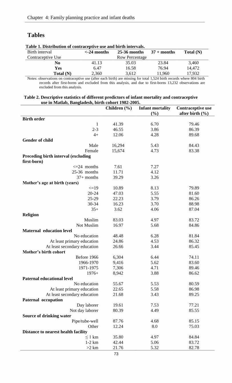
Chapter 4: Family planning practice and infant deaths
73
Tables
Table 1. Distribution of contraceptive use and birth intervals.
Birth interval <-24 months 25-36 months 37 + months Total (N)
Contraceptive Use Row Percentage
No 41.13 35.03 23.84 3,460
Yes 6.47 16.58 76.94 14,472
Total (N) 2,360 3,612 11,960 17,932 Notes: observations on contraceptive use (after each birth) are missing for total 1,524 birth records where 804 birth
records after first-borns and excluded from this analysis, and due to first-borns 13,232 observations are
excluded from this analysis.
Table 2. Descriptive statistics of different predictors of infant mortality and contraceptive
use in Matlab, Bangladesh, birth cohort 1982-2005.
Children (%) Infant mortality
(%)
Contraceptive use
after birth (%)
Birth order
1 41.39 6.70 79.46
2-3 46.55 3.86 86.39
4+ 12.06 4.28 89.68
Gender of child
Male 16,294 5.43 84.43
Female 15,674 4.73 83.38
Preceding birth interval (excluding
first-born)
<=24 months 7.61 7.27
25-36 months 11.71 4.12
37+ months 39.29 3.26
Mother’s age at birth (years)
<=19 10.89 8.13 79.89
20-24 47.03 5.55 81.60
25-29 22.23 3.79 86.26
30-34 16.23 3.70 88.98
35+ 3.62 4.06 87.04
Religion
Muslim 83.03 4.97 83.72
Not Muslim 16.97 5.68 84.86
Maternal education level
No education 48.48 6.28 81.84
At least primary education 24.86 4.53 86.32
At least secondary education 26.66 3.44 85.45
Mother’s birth cohort
Before 1966 6,304 6.44 74.11
1966-1970 9,416 5.62 83.60
1971-1975 7,306 4.71 89.46
1976+ 8,942 3.88 86.62
Paternal educational level
No education 55.67 5.53 80.59
At least primary education 22.65 5.58 86.98
At least secondary education 21.68 3.43 89.25
Paternal occupation
Day laborer 19.61 7.53 77.21
Not day laborer 80.39 4.49 85.55
Source of drinking water
Pipe/tube-well 87.76 4.68 85.15
Other 12.24 8.0 75.03
Distance to nearest health facility
≤ 1 km 35.80 4.97 84.84
1-2 km 42.44 5.06 83.72
>2 km 21.76 5.32 82.78

74
Table 3: Estimation Results.
Variable Contraceptive use Log birth space Infant mortality Prob (next birth)
Panel A parameter s.e parameter s.e parameter s.e Parameter s.e
Male -0.070 0.041 0.002 0.010 0.025 0.037 -0.031 0.045
Muslim -0.092* 0.042 -0.008 0.010 -0.023 0.052 0.602** 0.064
Birth order 0.057 0.071 0.084** 0.018 0.064 0.103 -0.072 0.086
Birth order square -0.011 0.010 -0.019** 0.002 -0.007 0.014 0.005 0.009
Mother’s age at birth (years)/10 0.005* 0.002 0.003** 0.001 -0.012** 0.003 -0.001 0.003
Mother’s age at birth/10 square 0.230** 0.047 0.048** 0.012 0.193** 0.060 0.228** 0.059
Maternal education level
At least primary education 0.116** 0.037 0.027** 0.008 -0.047 0.047 0.024 0.050
At least secondary education 0.181** 0.045 0.043** 0.010 -0.023 0.060 -0.366** 0.071
Mother’s birth cohort
1966-1970 0.565** 0.038 -0.007 0.009 -0.026 0.047 0.033 0.046
1971-1975 1.208** 0.0467 0.017 0.011 -0.133* 0.058 0.007 0.064
1976+ 1.841** 0.057 0.052** 0.012 -0.159* 0.069 0.574* 0.258
Paternal educational level
At least primary education 0.200** 0.037 -0.024* 0.008 0.056 0.044 -0.011 0.050
At least secondary education 0.291** 0.041 -0.024* 0.009 -0.205** 0.059 -0.129* 0.056
Father is day labourer 0.194** 0.052 -0.022 0.011 0.131* 0.055 -0.508** 0.064
No tubewell/piped water 0.052 0.037 0.031** 0.009 -0.163* 0.056 -0.100 0.053
Distance to health centre (in km) -0.009 0.015 0.006 0.003 0.005 0.020 -0.018 0.017
Lagged contraceptive use 0.495** 0.010
lagged infant mortality -0.880** 0.060 -0.554** 0.016 -0.020 0.072 -0.139 0.089
First boy surviving 0.528** 0.062 0.126** 0.016 -0.955** 0.105
First girl surviving 0.440** 0.063 0.085** 0.016 -0.873** 0.096
After first boy, # of boys surviving 0.353** 0.056 0.079** 0.015 -0.678** 0.085
After first girl, # of girls surviving 0.178** 0.052 0.027 0.015 -0.298** 0.072
Preceding log birth interval -1.586** 0.373
Preceding birth interval square 0.196** 0.052
Constant -0.226 0.293 2.899** 0.073 3.131** 0.750 4.472** 0.462
Panel B
Ρ 0.328 0.067 0.066 0.435
Correlation (row1) 0.184 -0.306 -0.727
Correlation (row2) -0.764
Correlation (row3) 0.205 -0.153
Notes: * 2 < t-value < 3; ** t-value ≥ 3
Reference category: gender is female, religion is Muslim, mother and father have no education, father is not day-labourer,
source of drinking water is tube-well/pipewater, and mother’s birth cohort before 1966.

Chapter 4: Family planning practice and infant deaths
75
Table 4. Simulation results.
Column 1 Column 2 Column
3 Benchmark Contraceptive
use
Contraceptive non-
use Birth interval 43.82 months +4.13 months -13.25 months
Number of births (fertility) 2.37 -2.43% +19.36%
Number of survivors 2.25 -2.28% +19.26%
For all children
Infant mortality 51.3/1000 -2.88% +1.62%
For children after first born
Infant mortality 39.6/1000 -7.86% +10.61%
Note: column1: Outcomes benchmark simulation, columns 2 and 3: deviations from the benchmark simulation if everyone uses
contraceptives (column 2) or noone uses contraceptives (column 3)
Table 5. Simulation results (alternative definition of contraceptives use).
Column 1 Column 2 Column 3
Benchmark Contraceptive use Contraceptive non-
use Birth interval 43.43 months +7.53 months -5.67 months
Number of births (fertility) 2.41 -6.01 % +8.65 %
Number of survivors 2.28 -5.93 % +8.72 %
For all children
Infant mortality (%) 51.0/1000 -1.48 % -1.13 %
For children after first born
Infant mortality (%) 39.4/1000 -6.89 % +1.44 %
Note: column1: Outcomes benchmark simulation, columns 2 and 3: deviations from the benchmark simulation if
everyone uses contraceptives (column 2) or noone uses contraceptives (column 3)

76
Figure
Note: 0 = non-use
1 = start one year after birth or later
2 = start within one year after birth and continue until more than one year after birth
3 = start within one year after birth and stop before one year after birth
4 = missing
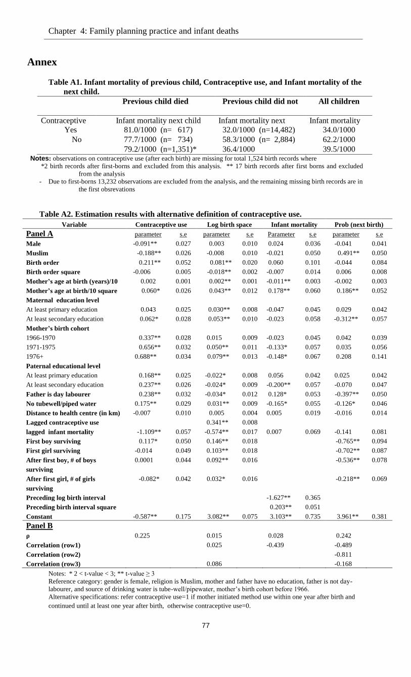
Chapter 4: Family planning practice and infant deaths
77
Annex
Table A1. Infant mortality of previous child, Contraceptive use, and Infant mortality of the
next child.
Previous child died
(n=1,353)
Previous child did not
die
(n= 17,383)
All children
(n=18,736)
Contraceptive
use
Infant mortality next child Infant mortality next
child
Infant mortality
next child Yes 81.0/1000 (n= 617) 32.0/1000 (n=14,482) 34.0/1000
No 77.7/1000 (n= 734) 58.3/1000 (n= 2,884) 62.2/1000
Total
79.2/1000 (n=1,351)* 36.4/1000
(n=17,366)**
39.5/1000 Notes: observations on contraceptive use (after each birth) are missing for total 1,524 birth records where
*2 birth records after first-borns and excluded from this analysis. ** 17 birth records after first borns and excluded
from the analysis
- Due to first-borns 13,232 observations are excluded from the analysis, and the remaining missing birth records are in
the first obsrevations
Table A2. Estimation results with alternative definition of contraceptive use.
Variable Contraceptive use Log birth space Infant mortality Prob (next birth)
Panel A parameter s.e parameter s.e Parameter s.e parameter s.e
Male -0.091** 0.027 0.003 0.010 0.024 0.036 -0.041 0.041
Muslim -0.188** 0.026 -0.008 0.010 -0.021 0.050 0.491** 0.050
Birth order 0.211** 0.052 0.081** 0.020 0.060 0.101 -0.044 0.084
Birth order square -0.006 0.005 -0.018** 0.002 -0.007 0.014 0.006 0.008
Mother’s age at birth (years)/10 0.002 0.001 0.002** 0.001 -0.011** 0.003 -0.002 0.003
Mother’s age at birth/10 square 0.060* 0.026 0.043** 0.012 0.178** 0.060 0.186** 0.052
Maternal education level
At least primary education 0.043 0.025 0.030** 0.008 -0.047 0.045 0.029 0.042
At least secondary education 0.062* 0.028 0.053** 0.010 -0.023 0.058 -0.312** 0.057
Mother’s birth cohort
1966-1970 0.337** 0.028 0.015 0.009 -0.023 0.045 0.042 0.039
1971-1975 0.656** 0.032 0.050** 0.011 -0.133* 0.057 0.035 0.056
1976+ 0.688** 0.034 0.079** 0.013 -0.148* 0.067 0.208 0.141
Paternal educational level
At least primary education 0.168** 0.025 -0.022* 0.008 0.056 0.042 0.025 0.042
At least secondary education 0.237** 0.026 -0.024* 0.009 -0.200** 0.057 -0.070 0.047
Father is day labourer 0.238** 0.032 -0.034* 0.012 0.128* 0.053 -0.397** 0.050
No tubewell/piped water 0.175** 0.029 0.031** 0.009 -0.165* 0.055 -0.126* 0.046
Distance to health centre (in km) -0.007 0.010 0.005 0.004 0.005 0.019 -0.016 0.014
Lagged contraceptive use 0.341** 0.008
lagged infant mortality -1.109** 0.057 -0.574** 0.017 0.007 0.069 -0.141 0.081
First boy surviving 0.117* 0.050 0.146** 0.018 -0.765** 0.094
First girl surviving -0.014 0.049 0.103** 0.018 -0.702** 0.087
After first boy, # of boys
surviving
0.0001 0.044 0.092** 0.016 -0.536** 0.078
After first girl, # of girls
surviving
-0.082* 0.042 0.032* 0.016 -0.218** 0.069
Preceding log birth interval -1.627** 0.365
Preceding birth interval square 0.203** 0.051
Constant -0.587** 0.175 3.082** 0.075 3.103** 0.735 3.961** 0.381
Panel B
ρ 0.225 0.015 0.028 0.242
Correlation (row1) 0.025 -0.439 -0.489
Correlation (row2) -0.811
Correlation (row3) 0.086 -0.168
Notes: * 2 < t-value < 3; ** t-value ≥ 3
Reference category: gender is female, religion is Muslim, mother and father have no education, father is not day-
labourer, and source of drinking water is tube-well/pipewater, mother’s birth cohort before 1966.
Alternative specifications: refer contraceptive use=1 if mother initiated method use within one year after birth and
continued until at least one year after birth, otherwise contraceptive use=0.
Chapter 5
Cause-specific neonatal deaths: levels, trend and
determinants in Rural Bangladesh, 1987-200515
5.1 Introduction
Of the 130 million children born alive each year worldwide, about four million die in the first
four weeks after birth. 99% of these deaths occur in low and middle income countries; 4% occur
in Bangladesh (Lawn et al. 2005). Achieving the fourth Millennium Development Goal (MDG-4)
of reducing under-5 child mortality by two-thirds between 1990 and 2015 remains one of the
United Nations’ global priorities (United Nations 2001). The recent trends in mortality suggest
that without substantial reductions in neonatal mortality, MDG-4 will not be achieved (Lawn et
al. 2005). Global reviews suggest that almost 60% of childhood deaths can be prevented by
increasing the coverage of existing newborn and child health interventions (Jones et al. 2003).
The information on causes of neonatal and child death is important here, since - it can be used to
prioritize and to increase the effectiveness of disease-specific interventions (Baqui et al. 2001;
Lawn et al. 2006).
Reducing neonatal mortality is a particularly important issue in Bangladesh. Although
child mortality rates in Bangladesh declined sharply during the last decades of the previous
century, the reduction is slowed down particularly in the neonatal period. Among child deaths,
those that occur during the first month represent an increasing proportion. Estimates based upon
the Bangladesh Demographic and Health Survey (BDHS) suggest that 70% of all under-five
deaths occur in the first year of life and 80% of these occur in the neonatal period (see Figure 1).
It is therefore a significant challenge to reduce neonatal mortality in order to meet MDG-4 of
reducing under-five mortality from 133 per 1,000 live births to two-thirds between 1990 and
2015. This study analyzes the levels and the trend of cause-specific neonatal deaths in
Bangladesh and associated risk factors, both observed and unobserved. The findings may help to
design policies that reduce neonatal mortality in Bangladesh in particular, but also are potentially
relevant for many other countries in the developing world.
15
This chapter is joint work with Arthur van Soest, Tilburg University and Govert E. Bijwaard, Netherlands
Interdisciplinary Demographic Institute (NIDI). We thank the members of committee for their valuable comments
that helped to improve the paper.
Chapter 5. Cause-specific neonatal deaths
79
We estimate a flexible competing risks model of causes of death until 28 days after birth
(neonatal deaths), considering children who survive the neonatal period as censored observations.
Our modelling approach is more flexible than in many existing studies of determinants of causes
of deaths. It combines a piecewise constant baseline hazard with proportionality assumptions
concerning the influence of observed and unobserved risk factors for each cause of death. The
model allows the unobserved heterogeneity components in the hazard rates for the various causes
of death to be correlated.
Our estimations are based upon prospective panel data from the Matlab region in
Bangladesh, following mothers and children over time from 1987 until 2005. Two sets of
villages are covered: an intervention area with non-standard health services (International Centre
for Diarrhoeal Disease Research, Bangladesh or ICDDR,B area), and an area with standard
government-provided health care facilities (comparison area); the differences between the two
areas give insight into how the additional health care services shape the child health
epidemiology over the period.
5.2 Background
The disease structure of neonatal deaths is different from that of post-neonatal deaths or deaths
of children older than one year (Bhatia 1989). Neonatal deaths are associated with biological
characteristics of the mother and with problems during pregnancy and child birth, which can be
improved by targeted interventions such as tetanus toxoid to pregnant women, nutrition
education, and increasing use of antenatal care, or by ensuring safe delivery. On the other hand,
socio-economic and programmatic factors that focused on reducing post-neonatal and child
deaths become more important during the post-neonatal period, when deaths are more often
caused by infectious diseases or accidents. For example, it is obvious that immunization of the
children or oral rehydration therapy will not prevent deaths during the neonatal period. It is,
therefore, more useful to work with separate models for the determinants of competing risks of
neonatal and post-neonatal death. In this study, we only consider the neonatal period.
In many countries, information on causes of death is not available. Verbal autopsy (VA)
is a tool used in a retrospective interview with family members about the circumstances of a
death to ascertain the underlying cause of death (Chen et al. 1980; Bhatia 1989; Baqui et al 2001;
Karar et al. 2009). The interview is usually held 22 days after the date of death with the mother,
or a close relative or neighbour in absence of the mothers (Karar et al. 2009). VA is not often
used because it can be prohibitively expensive or difficult. The Health and Demographic
Surveillance System (HDSS) of ICDDR,B in Matlab, Bangladesh, however, routinely records all
births, deaths and causes of deaths through VA for a total population of about 220,000
(ICDDR,B 2006). It also incorporates information on several indicators of socioeconomic status
of each household. The Matlab HDSS plays an important role in providing accurate information
on vital events (e.g. births, deaths) and causes of death that are not often available in many
resource-constrained setups.

80
In 1977, ICDDR,B started to provide extensive maternal-child health and family planning
(MCH/FP) services, in addition to existing government health services, in half of the HDSS area
called ICDDR,B area. The other half, called the comparison area, continued to get only the
standard government health services. The MCH/FP project includes provision of domiciliary
family planning services, simple nutrition education, tetanus toxoid immunization for pregnant
women (which was modified in 1981 to include all women of reproductive age), community-
based oral rehydration therapy, and measles immunization. These services were introduced
incrementally phase by phase (Phillips et al 1984). In the ICDDR,B area there are several
ICDDR,B sub-centres providing treatment for minor illnesses and, basic emergency obstetric
care (EOC), and a permanent hospital that provides treatment for diarrhoeal diseases. In order to
understand the way in which better health services shape child health, we analyze the data from
the area with the better health care services in addition to the government health services
(ICDDR,B area) as well as the data from an area with standard government health services only
(the comparison area - a typical rural area of Bangladesh).
Most of the studies of cause-specific neonatal deaths in developing countries, including
those in Matlab, Bangladesh, reported neonatal mortality rates by age-group, giving insight in
when and why the child deaths occur (Chen et al. 1980; Bhatia 1989; Baqui et al. 2001; Lawn et
al. 2006; Karar et al. 2009; Chowdhury et al. 2010). The trends in mortality, however, reveal that
factors other than the health and family planning interventions influence the levels of mortality in
the ICDDR,B and comparison areas (Bhatia 1989). To strengthen the targeting of interventions,
it may therefore be important to analyze what characterizes families and children at risk of
neonatal death due to various causes. In other words, what are the underlying factors that are
associated with cause-specific deaths? Our study contributes to answering this question.
The analysis of cause-specific death is related to the concept of competing risks
(Cornfield 1957; Fine and Gray 1999; Coviello and Boggess 2004). In a competing risk situation,
the analysis of one specific cause of death has to account for competing causes of death. For
example, in one study it was found that the probability of a female developing cancer at some
point during her life has increased by 25 per cent over a seven years period, but the largest part
of this increase was accounted for by decreases in other causes of mortality (Goldberg et al.
1956). To our knowledge, our study is the first that applies this type of model to neonatal
mortality Bangladesh.
Duration models are often used in demographic and epidemiological research where the
events to be modelled are associated with time, such as time till marriage, time from marriage till
birth of the first child, or time till death (Cox 1959; Heckman et al. 1985). Analyzing the
duration to competing causes of death leads to knowledge about when (time) and why (disease
types) deaths occur, which is useful for targeting policies of early prevention.
Studies of child deaths have shown that survival chances of several children in a family
are correlated and that variation in death risks across families remains after controlling for
Chapter 5. Cause-specific neonatal deaths
81
observed covariates (such as age of mother at birth, gender of the child, or race), and can be
attributed to unobserved family level heterogeneity. Examples are adverse genetic traits, inability
to take care of the child (behavioural factors), or (unobserved) environmental factors (Mosley
and Chen 1984; DasGupta 1990; Arulampalam and Bhalotra 2006).This is also relevant for
specific causes of death. For example, if a mother has a propensity to give birth to children with
too low birth weight, it may well happen that all births to this same mother expose too low
weight at birth (genetic traits). Furthermore, closely spaced births of the same mother may be
affected by infectious diseases of siblings (disease contamination) or environmental factors such
as unsafe water supply or limited access to health care. Finally, as emphasized by DasGupta
(1990), some mothers may be less resourceful in caring for their child than others, reflecting a
behavioural effect.
5.3 Data We combined the HDSS data of all live births and deaths of children for the ICDDR,B and
comparison area obtained between 1987 and 2005. The data set has records of 107,367 singleton
live births (57,830 from the comparison area and 49,837 from the ICDDR,B area) and 4,047
neonatal deaths and their causes (2,446 from the comparison area and 1,601 from the ICDDR,B
area). Data on education of both mother and father, occupation of the father, and source of
drinking water were obtained from the 1996 and 2005 census. For our purposes, we model the
two areas separately.16
5.3.1 Causes of death
Since 1966 HDSS has recorded data on causes of death, with particular emphasis on child and
maternal deaths. Before 1987, the cause of death was assigned by the health assistant, but from
1987 onwards the death form was revised and read by physicians who assigned a cause of death.
A single three-digit code was selected from a list of 97 possible codes derived from the ‘basic
tabulation list’ of the World Health Organization International Classification of Diseases,
Injuries and Causes of Death (World Health Organization 1977). The death of a child often has
more than one cause. The assignment of cause of death followed a hierarchical process whereby
certain diagnoses were viewed as more certain than others, and thus given priority as primary
and underlying cause of death. The assignment of causes of death is described details in the
literature (see for example, Fauveau et al. 1994; Adjuik et al. 2006; Lawn et al. 2006; Karar et al.
2009; Ronsmans et al. 2010).
For our statistical analysis, to reduce the sampling error resulting from small numbers, the
causes of neonatal deaths are first recoded into two categories (1) communicable diseases (CDs):
acute respiratory infections, diarrhoea, dysentery, sepsis, meningitis, hepatitis, chicken pox, and
16
Our primary interest of this research is to investigate the trends, pattern and determinants of epidemiological shifts
in the ICDDR,B area and the comparison area. Some efficiency could possibly be gained by analyzing the two areas
jointly, but this would also require at least some interactions of covariates with an area dummy (similar to one of the
sensitivity checks in chapter 2). We tried this but encountered convergence problems.

82
neonatal tetanus or Extended Program on Immunization (EPI) related diseases and other viral
diseases, (2) non-communicable diseases (NCDs): preterm delivery/low birth weight(LBW),
deaths related to neonatal conditions (birth asphyxia, birth trauma/cord haemorrhage, congenital
abnormality, neonatal infections, obstetric complications of new born, sudden infant death,
unspecified neonatal death and miscellaneous neonatal deaths). Second, for an analysis at a more
disaggregate level, exits due to non-communicable diseases (NCDs) of neonatal deaths were split
into three categories: (1) LBW: preterm delivery/low birth weight, (2) NCs: deaths related to
neonatal conditions (BA: birth asphyxia, CA: congenital abnormality or birth trauma/cord
haemorrhage, NEO: neonatal related other conditions, OBSCOMP: obstetric complications), (3)
Other (sudden infant death/unspecified or miscellaneous). See Table 1 in the annex for further
details.
5.3.2 Socio-demographic variables
The covariates in the model refer to gender of the child, child birth cohorts (1987-1992, 1993-
1999 or 2000-2005), religion of the family (Muslim or Hindu), dummies for birth order,
education of the parents, employment status of the mother and occupation of the father (day
labourer or not), source of drinking water (piped water or not), the mother’s age at birth, and the
distance to the nearest health facility. Maternal education is a proxy of child care skills and the
ability to use modern health care services. Both paternal education and occupation are considered
here as household socioeconomic indicators. The birth cohort of child can capture the time trends
of cause-specific mortality risks. The distance variable captures the availability of health services,
and sources of drinking water the environmental effects. Birth order variables are included to
capture sibling effects on the risks of cause specific mortality. Summary statistics of these
variables are presented in Table 1.
5.3.3 Distribution of causes of deaths
Table 2 depicts the percentage distribution of causes of neonatal death in the neonatal period (0-
28 days). Of all neonatal deaths recorded in Matlab during 1987-2005, deaths due to NCDs
comprised 87% and 78% in the ICDDR,B and comparison areas, respectively. The specific
types of NCDs demonstrate that prematurity or low birth weight is a leading cause of death,
followed by deaths ‘unable to specify’. Among deaths due to CDs, the majority were due to
acute respiratory infections (10.79 and 15.35 percent).
Figures 2 and 3 demonstrate that over the period 1987-2005, the fraction of neonatal
deaths due to prematurity or low birth weight decreased, particularly in the ICDDR,B area. The
fraction of deaths due to miscellaneous causes (sudden infant death, unable to specify, other
disorders originated in the perinatal period etc.) also fell over time. Figures 4 and 5 show that
deaths due to acute respiratory infections form an inreasing share of death due to communicable
diseases in the comparison area, with neonatal tetanus or EPI related deaths disapprearing in
both areas.
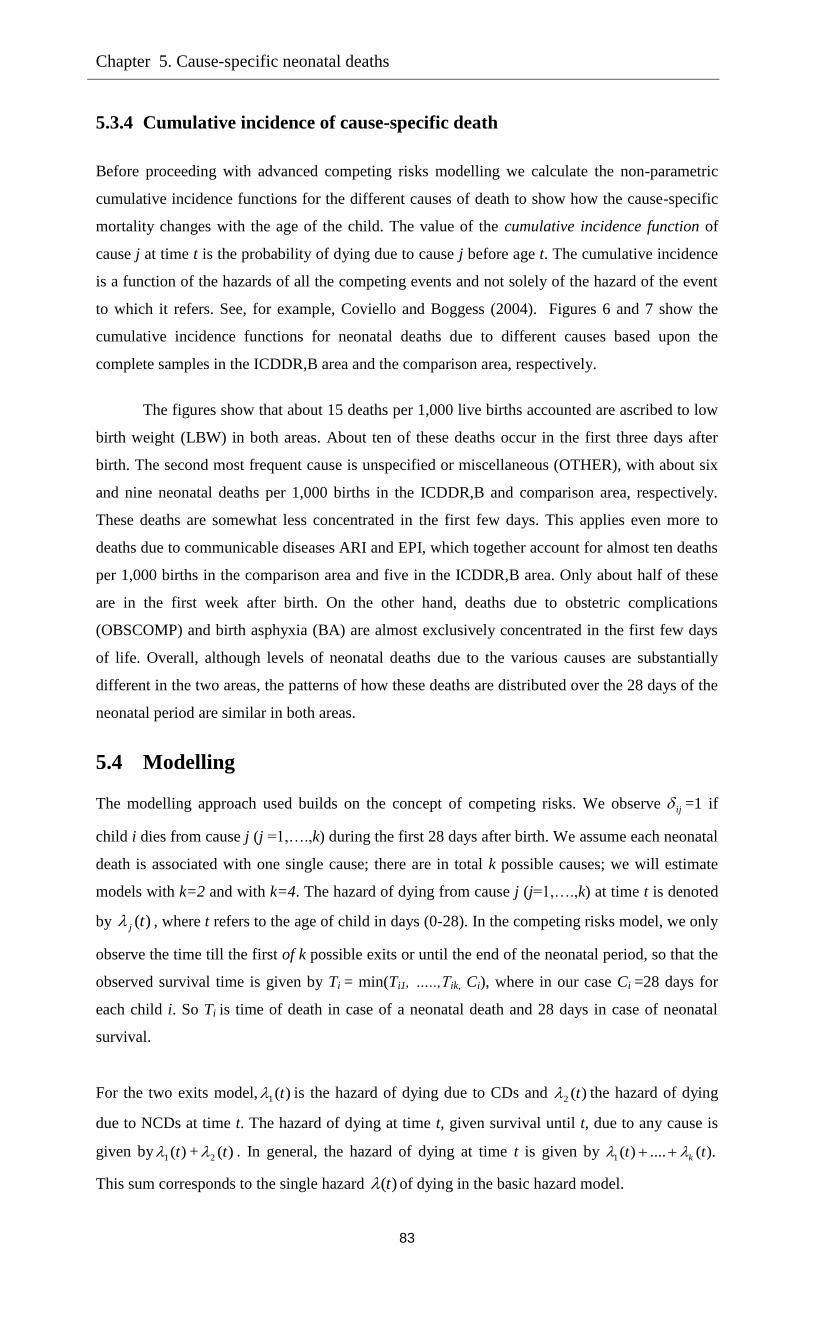
Chapter 5. Cause-specific neonatal deaths
83
5.3.4 Cumulative incidence of cause-specific death
Before proceeding with advanced competing risks modelling we calculate the non-parametric
cumulative incidence functions for the different causes of death to show how the cause-specific
mortality changes with the age of the child. The value of the cumulative incidence function of
cause j at time t is the probability of dying due to cause j before age t. The cumulative incidence
is a function of the hazards of all the competing events and not solely of the hazard of the event
to which it refers. See, for example, Coviello and Boggess (2004).
Figures 6 and 7 show the
cumulative incidence functions for neonatal deaths due to different causes based upon the
complete samples in the ICDDR,B area and the comparison area, respectively.
The figures show that about 15 deaths per 1,000 live births accounted are ascribed to low
birth weight (LBW) in both areas. About ten of these deaths occur in the first three days after
birth. The second most frequent cause is unspecified or miscellaneous (OTHER), with about six
and nine neonatal deaths per 1,000 births in the ICDDR,B and comparison area, respectively.
These deaths are somewhat less concentrated in the first few days. This applies even more to
deaths due to communicable diseases ARI and EPI, which together account for almost ten deaths
per 1,000 births in the comparison area and five in the ICDDR,B area. Only about half of these
are in the first week after birth. On the other hand, deaths due to obstetric complications
(OBSCOMP) and birth asphyxia (BA) are almost exclusively concentrated in the first few days
of life. Overall, although levels of neonatal deaths due to the various causes are substantially
different in the two areas, the patterns of how these deaths are distributed over the 28 days of the
neonatal period are similar in both areas.
5.4 Modelling
The modelling approach used builds on the concept of competing risks. We observe ij =1 if
child i dies from cause j (j =1,….,k) during the first 28 days after birth. We assume each neonatal
death is associated with one single cause; there are in total k possible causes; we will estimate
models with k=2 and with k=4. The hazard of dying from cause j (j=1,….,k) at time t is denoted
by )(tj , where t refers to the age of child in days (0-28). In the competing risks model, we only
observe the time till the first of k possible exits or until the end of the neonatal period, so that the
observed survival time is given by Ti = min(Ti1, …..,Tik, Ci), where in our case Ci =28 days for
each child i. So Ti is time of death in case of a neonatal death and 28 days in case of neonatal
survival.
For the two exits model, )(1 t is the hazard of dying due to CDs and )(2 t the hazard of dying
due to NCDs at time t. The hazard of dying at time t, given survival until t, due to any cause is
given by )(1 t + )(2 t . In general, the hazard of dying at time t is given by 1( ) .... ( ).kt t
This sum corresponds to the single hazard ( )t of dying in the basic hazard model.

84
The hazard rates are specified as the following mixed proportional hazards (see for example
Manton et al. 1981 or Lancaster 1979):
0( | , ) ( )exp( ) , 1,...,j j j j jt x v t x v j k (1)
The hazard rates are functions of time t, explanatory variables which in our case do not vary
over the neonatal period (child, mother and community level observed characteristics), and time
constant mother-specific heterogeneity jv . The explanatory variables x are assumed to enter
through linear indexes , 1,..., .jx j k Time dependence is incorporated with a piecewise
constant baseline hazard0 ( ) :j t for each cause of death j (j=1,…,k), we have )(0 tj =
0
1
exp( ) exp( ) ( )H
j hj h
h
I t
with )(tI h = 1[ ]h hI t t t , the indicator function for the interval 1[ , ]h ht t ,
and t 0 = 0, tH
= 28 days. Any duration dependence can be approximated arbitrarily closely by
increasing the number of intervals. We experimented with several partitions of [0, 28] into
several intervals and found the best model performance for the H=5 intervals [0,1), [1,2), [2-3),
[3,7) and [7,28]. For identification we need to restrict one of the hj (h=1,…,H) to zero for each j.
We choose . Thus, 0 j determines the hazard in the last interval. The other hj determine
the ratio of the hazard in each interval compared to this last interval. The baseline hazard at
1[ , )h ht t t is higher than the baseline hazard for a duration of ht t if 0h and lower if
0h .
Our emphasis is on the specification of unobserved heterogeneity , 1,...jv j k , capturing
unobserved factors that affect survival of a child. Ignoring these factors may bias the parameter
estimates. In principle, unobserved heterogeneity can be child specific, mother specific, or
community specific. Following several existing studies emphasizing the role of mother specific
heterogeneity or ‘frailty,’ (Sastry 1997; Arulampalam and Bhalotra 2006) we model mother
specific heterogeneity only. The unobserved heterogeneity terms 0jv are time-independent and
independent of observed characteristics x. Many different choices for the distribution of the
unobserved heterogeneity exist. One issue is that the unobserved heterogeneity terms jv of
different causes of death j can be correlated. To address this we adopt a two factor loading model,
with two independent fundamental factors 1W and 2W both having a discrete distribution on {-
1,1}. This implies that
v j = exp( 11Wj + 22Wj ) , j=1,…,k (2)
Let W= ( 1W , 2W )' and let A be the matrix of factor loadings with rows A j =( 1j , 2j ). Then
the covariance matrix of the logarithms of the unobserved heterogeneity terms , ...,1( )kv v v is
given by V(ln(v)) = AV(W)A'. One additional restriction is needed for identification, we choose
12 =0. The probabilities for the discrete distributions for 1W , 2W are Pr( 1W = -1)= 1p and

Chapter 5. Cause-specific neonatal deaths
85
Pr(2W = -1)=
2p . We assume for both 1p and
2p a logit form, i.e. 1p = e
θ1/(1+ e
θ1) and
2p =
eθ2
/(1+ eθ2
) and we estimate the θ’s. Thus, for example, for our model with two exits (CDs and
NCDs) the unobserved heterogeneity terms have the following distribution:
1 2 2 22 1 2
1 2 2 22 1 2
1 2 2 22 1 2
1 2 2 22 1 2
(ln , ln ) ;
(ln , ln ) (1 );
(ln , ln ) (1 ) ;
(ln , ln ) (1 )(1 ).
P v v p p
P v v p p
P v v p p
P v v p p
The parameters can be estimated jointly with maximum likelihood in Stata; details on the
likelihood function are available upon request. The covariance matrix of the unobserved
heterogeneity terms can be estimated ex post, since it is a function of model parameters. This
also applies to the total survival and cumulative incidence functions. The total survival function
conditional on observed and unobserved heterogeneity is
= Pr
= exp (3)
The cumulative incidence function of cause j is the probability of dying due to cause j before age
t. In section 3, we have already presented the empirical cumulative incidence functions for
various causes for the complete samples in the two areas. Based upon the model, we can also
estimate the cumulative incidence functions for specific mothers, that is, conditional on observed
and unobserved heterogeneity. They are given by:
= (4)
Integrating out the observed and unobserved heterogeneity, we can also obtain the total survival
and cumulative incidence functions. Note that the sum of all cumulative incidence functions at a
given age is equal to one minus the total survival function at that age, i.e.
.
5.5 Estimation results
5.5.1 Communicable versus Non-communicable diseases: Covariate effects
Tables 3 and 4 present the estimation results for the models distinguishing two causes of death
(non-communicable (NCDs) and communicable diseases (CDs)) in the ICDDR,B area and the
comparison area, respectively. Tables 5 and 6 present the results for the same models with four
causes of death, distinguishing CDs and three types of NCDs: low birth weight (LBW), neonatal
related conditions (NCs), and unspecified/other (Other). We focus on the competing risk model
introduced in the previous section, controlling for observed covariates in all the hazards and for
mother specific unobserved heterogeneity terms that are allowed to be correlated across causes.
For comparison, Tables 3 and 4 also present the parameter estimates of standard hazard models
without unobserved heterogeneity for each cause of death separately (“traditional model”; first
column in each table). In general, the estimated effects of the covariates are similar in the
traditional model and in the full model, in terms of sign, size, and significance level. Allowing

86
for a general form of unobserved heterogeneity therefore has very little effect on the estimated
duration dependence (the coefficients in the baseline intensity) or the estimated effects of the
exogenous variables.
Tables 3 and 4 show that, in both areas, male children are more likely to die of CDs or
NCDs than female children in similar families and circumstances. The gender differences are
larger and more significant in the ICDDR,B area, and, in relative terms, larger for CDs than for
NCDs. The magnitude of the differences is substantial. For example, in the ICDDR,B area, the
chances of dying of a communicable disease on a given day in the neonatal period are about 70%
higher (exp(0.54)-1)*100%) for a boy than for a girl (ceteris paribus). For a reference individual
this is a difference of about 11 deaths per 1,000 over the complete neonatal period.
Religion, father’s occupation and distance to the nearest health facility play no significant
role in the ICDDR,B area. In the comparison area, however, a child is significantly more likely
to die due to a CDs if the mother is Hindu (rather than Muslim), if the father is a day labourer, or
if the distance to the nearest health facility is larger. The latter also applies to NCDs. It seems
plausible that distance to the nearest health facility is more important in the comparison area than
in the ICDDR,B area, since distances are much larger in the comparison area (cf. Table 1),
making limited access to a health facility a more common concern there (Bhatia 1981).
A higher education level of the mother significantly reduces the NCDs hazard in both
areas, whereas it has a negative but insignificant effect on death due to CDs. On average, if the
mother is educated up at least secondary level this reduces the number of deaths per 1,000 live
births due to NCDs on the first day after birth by 9 in the ICDDR,B area and by 14 in the
comparison area.
In line with the demographic literature, first born children and children born to mothers
aged less than 20 years old are at higher risk of neonatal mortality compared to the reference
categories (20-24 years old mother and higher order births). The differences are much larger and
more significant for NCDs than for CDs. In the ICDDR,B area, there is some evidence that
children of older mothers (age 25 and older) have a lower risk of dying from CDs than the
benchmark category (ages 20-24). There are no significant differences amongst birth orders 2 or
higher.
A decreasing trend of neonatal death is observed in both CDs and NCDs in both areas,
but it is not always significant. The degree of decline is strongest for CDs in the comparison area,
where the risk has fallen substantially in the period 2000-2005. In the ICDDR,B area, there has
been a significant reduction in the risk due to NCDs from the first to the second time period
considered (a reduction of more than 25% from 1987-1992 to 1993-1999). In the comparison
area, a similar reduction occurred a few years later.
A monotonically decreasing pattern trend is observed in the baseline intensity of dying
due to NCDs in both areas: the hazard of dying is largest on the day of birth and already much

Chapter 5. Cause-specific neonatal deaths
87
lower one day after birth, and decreases further during the neonatal period. On the other hand,
the pattern is quite different for communicable diseases, for which the hazard declines much less
during the first week (and even increases from day 0 to day 1). This difference is in line with
Figures 6 and 7, where we already saw that deaths due to CDs less often occurred on the first few
days after birth.
5.5.2 CDs and NCDs: Unobserved heterogeneity
The bottom panels of Tables 3 and 4 show that there is evidence of unobserved heterogeneity in
both areas. In the ICDDR.B area, the covariance between the (mother specific) unobserved
heterogeneity terms in the two competing hazards is significantly positive, implying a correlation
coefficient of 0.28. In the comparison area the implied correlation is 0.66, but the estimated
covariance is not significant. In both areas, only one of the variances is significantly different
from zero, suggesting that it is hard to identify the covariance structure of the unobserved
heterogeneity terms, possibly due to the fact that, fortunately, neonatal death due to each of the
specific causes is not such a common event and more than one neonatal death in the same family
is rare.
5.5.3 Model with four causes of death: Covariate effects
In order to get a better understanding of the deaths due to NCDs, we also split NCDs into three:
(1) low birth weight (LBW); (2) neonatal conditions (NCs) which includes CA, NEO, BA,
OBSCOMP; and (3) Other: sudden infant deaths/ unspecified or miscellaneous (miscellaneous:
with a range of 27-30 cases in each area). Together with CDs, this gives four different causes of
neonatal death. The results of these models for the complete model allowing for correlated
unobserved heterogeneity in all four hazard rates are reported in Tables 5 and 6 for the ICDDR,B
area and the comparison area, respectively. (Results of the corresponding traditional models
generally give similar effects for the covariates; details are available upon request from the
authors.) In general, the effects of many covariates are quite different for the three causes of
death due to non-communicable diseases, showing that treating these causes separately is
worthwhile.
The disadvantage for boys in NCDs that we already found in Tables 3 and 4 can be
attributed to their larger vulnerability to NCs and, in the ICDDR,B area, to death due to low birth
weight. We find no significant difference between boys and girls for the category “Other.” As in
Table 3, no significant religion difference is found in the ICDDR,B area. In the comparison area,
however, a child born to a Hindu mother is not only more likely than an otherwise similar child
from a Muslim mother to die from a communicable disease, but is also more vulnerable to death
related to NCs.
In both areas, higher education of the mother substantially reduces the risk of death due to
LBW. The effects of mother’s education on the other causes of death are much weaker, though
some are still significant at the 5% level. Children born to very young mothers (age less than 20

88
years) are more likely to die due to LBW and due to “other” causes in both areas. The effects of
birth order show that first born children are at higher risk of death due to any cause than higher
order births. The differences are large, sometimes more than a factor two; the only exception is
death due to CDs in the ICDDR,B area where birth order appears to play no role.
Some of the results for the father’s education level and type of occupation seem puzzling
at first sight. In particular, we find that children of fathers with primary education rather than no
education have higher risk to die because of NCs in both areas, and the effect is significant at the
5% level (but not at 1%). Moreover, if the father is a day labourer, this reduces the risk to die
from NCDs in the ICDDR,B area, whereas being a day labourer is a negative index of socio-
economic status. The finding that death due to NCs is positively associated with socio-economics
status is in line, however, with data from the nationally representative BDHS 2004 (NIPORT et
al. 2005), which show that deaths due to birth asphyxia are more common amongst mothers with
higher education. An existing study (Chowdhury et al. 2010) suggests this may be related to
delivery at a health centre instead of at home, and this finding is in line with large unobserved
heterogeneity for deaths due to NCs and increased institutional delivery (which includes mainly
birth asphyxia/neonatal infections and delivery complications) in the ICDDR,B area.17
On the
other hand, secondary education of the father reduces the risk to die from “other” causes in the
comparison area, and in the same area, being a day labourer increases the risk of death due to
CDs (as in Table 4), as expected.
Lack of access to running water has the expected effect of increasing mortality due to
CDs in the ICDDR,B area. It also increases the risk of dying from LBW. On the other hand, it
has no significant effects in the comparison area. In the comparison area, a larger distance to the
nearest health centre increases the risk of CDs related death (as in Table 4) and of LBW related
death. As in Table 3, it has no significant effect in the ICDDR,B area where distances are smaller.
In both areas, we find substantial differences among cohort effects for different causes of death.
In particular, the risk of NCs related death has increased in 2000-2005 compared to 1987-1999,
while the risk of dying from the other causes has fallen. Particularly for the “other” category
(which includes sudden infant deaths, among others) the reduction in the period 2000-2005 is
remarkably large in both areas.
The baseline intensities of dying due to LBW, NCs, and other non-communicable
diseases follow similar patterns, which are also similar to the patterns in Tables 3 and 4 for all
NCDs combined: the risk is very high on the first day of life, and reduces quickly after a few
days. The pattern is quite different from that for non-communicable diseases, for which the
hazard shows a much less clear duration dependence pattern over the neonatal period, as we
already saw in Tables 3 and 4.
17
A study in Matlab revealed that 19% of births took place in ICDDR,B facilities, 4% occurred in other (public and
private) facilities, 2.6 births were attended by ICDDR,B midwives at home, and the remaining deliveries took place
at home (Anwar et al. 2004). However, according to BDHS 2004, nationally 90% of all births took place at home,
which is comparable with our comparison area, a typical rural area of Bangladesh with the usual standard health
facilities.

Chapter 5. Cause-specific neonatal deaths
89
5.5.4 Model with four causes of death: Unobserved heterogeneity
We find some evidence of unobserved heterogeneity: two of the four variances are significant in
the ICDDR,B area and one in the comparison area. Moreover, in the ICDDR,B area, the
covariance between the unobserved heterogeneity terms in the hazards for communicable
diseases and low birth weight related deaths is significant at the 1% level. The other covariances
are insignificant at the 5% level. Still, at least in the ICDDR.B area, the covariance matrix of the
unobserved heterogeneity terms seems easier to estimate in this model than in the model with
only two causes of death – we no longer find the very large standard error found for NCDs in
Table 3. This suggests that this large standard error might be due to aggregation of rather
different causes of death. (That this problem does not arise in the comparison area may be
because of the larger death rates there.)
5.5.5 Cumulative incidences functions
The cumulative incidence functions corresponding to the models with four causes of death for
the benchmark cases are shown in Figures 8 (ICDDR,B area) and 9 (comparison area). These
rates are substantially different from the rates for the complete sample (see Figures 6 and 7),
since the socio-economic characteristics of the benchmark case are not representative for the
sample average. The patterns over time confirm what we concluded from the baseline hazards in
Tables 5 and 6: they are much steeper in the first few days for the various types of non-
communicable diseases than for communicable diseases. At each point of time, the cumulative
number of deaths due to LBW is larger than the numbers for all three other causes. In the
ICDDR,B area, about 16 deaths per 1,000 live births are due to LBW within one day after birth,
rising to about 28 per 1,000 after 28 days. The patterns over time are similar in the two areas, but
the levels are not: the hazards for CDs and for “other” NCDs are much larger in the comparison
area than in the ICDDR,B area.
Figures 10 and 11 show the same cumulative incidence functions as Figures 8 and 9, but
now for a benchmark birth in the period 2000-2005 instead of 1987-1992. The epidemiological
shifts are similar in the two areas. In both areas, the largest difference between the two time
periods is the significant reduction of the number of deaths due to LBW, about 12 per 1,000 in
the ICDDR,B area and 8 per 1,000 in the comparison area during the whole neonatal period, and
concentrated in the first few days after birth. On the other hand, the number of deaths due to
NCs surprisingly increases substantially in the period 2000-2005, by about 5-6 deaths per 1,000
live births compared to the reference period 1987-1992. In the competing risks situation, the
decrease of deaths due to LBW is perhaps partly substituted by an increase of deaths due to
neonatal infections or obstetric complications at birth.

90
5.6 Discussion and conclusion
This study analyzes causes of neonatal death, derived from open-ended death history data
reported by the mother or a close relative or neighbour (in absence of the mother) and recorded
by non-medically trained field workers. Three physicians independently reviewed all death
records and reached consensus. The uniform death registration form and assessment of causes of
death by physicians during 1987-2005 is an important strength for the comparison the patterns of
causes of death over the years. This Verbal Autopsy method was recommended by WHO to
attain the reliable epidemiological data on mortality (Fauveau at el. 1994; Bryce et al. 2005).
During 1987-2005, recorded neonatal mortality per 1,000 live births was 32.3 in the
ICDDR,B area (which, in addition to government services, gets high quality health care services)
and 42.3 in the comparison area (with standard government services). In Bangladesh, the
national neonatal mortality rate is about 41 per 1,000 live births (BDHS, 2004) and this rate is
close to the rate of comparison area, a typical setup in rural Bangladesh.
A remarkable success is the reduction in the number of neonatal deaths due to neonatal
tetanus or EPI, which mainly explains the reduction of total neonatal mortality in ICDDR,B area,
and which is well noticed in other studies (Bhatia 1989; Baqui et al. 2001). This is supported by
the cause-of-death data, indicating that mortality rates due to neonatal tetanus were 1.0% and
5.9% per 1,000 live births in ICDDR,B and comparison areas, respectively. During the study
period, low birth weight was the foremost leading cause of neonatal deaths in both ICDDR,B and
comparison area. Our findings are in agreement with global findings pointing at preterm birth or
low birth weight as a major cause of neonatal death in the world and particularly in Bangladesh
(Lawn et al. 2006).
On the other hand, death related to NCs - mainly neonatal infections or obstetric
complications - became a primary cause of neonatal death in both areas in 2000-2005 (see also,
Chowdhury et al., 2010). Compared to the 1987-1992 period, for otherwise similar children, the
hazard to die due to NCs increased by about 77% in the ICDDR,B area and 46% in the
comparison area. The increase in this rate in the ICDDR,B area is remarkable. As indicated in an
earlier study, the absence of appropriate antenatal, intra-partum, and postnatal care in both areas
takes an unnecessary toll on infant lives, which could easily be prevented with appropriate
interventions (Bhatia 1989; Bari et al. 2002; Bang et al. 2005; Velaphi and Pattinson 2007).
Although a downward trend since 1993 is observed in neonatal death due to NCDs in
both areas, this decline is faster in the ICDDR,B area, specifically for deaths due to LBW. This
finding can be related to the large scale nutrition programs in the ICDDR,B area, which attempt
to improve nutrition of pregnant mothers with the goal of increasing birth weight (see
www.icddrborg/what-we-do/health-programmes/nutrition). Since villages in the comparison area
are contiguous to those in the ICDDR,B area, spill-over effects of these programs, changing
information and behaviour in the comparison area also, may explain why mortality due to LBW
has also significantly declined in the comparison area (Phillips et al. 1988).
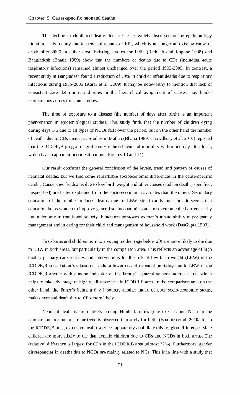
Chapter 5. Cause-specific neonatal deaths
91
The decline in childhood deaths due to CDs is widely discussed in the epidemiology
literature. It is mainly due to neonatal tetanus or EPI, which is no longer an existing cause of
death after 2000 in either area. Existing studies for India (Reddiah and Kapoor 1988) and
Bangladesh (Bhatia 1989) show that the numbers of deaths due to CDs (including acute
respiratory infections) remained almost unchanged over the period 1993-2005. In contrast, a
recent study in Bangladesh found a reduction of 79% in child or infant deaths due to respiratory
infections during 1986-2006 (Karar et al. 2009). It may
be noteworthy to mention that lack of
consistent case definitions and rules in the hierarchical assignment of causes may hinder
comparisons across time and studies.
The time of exposure to a disease (the number of days after birth) is an important
phenomenon in epidemiological studies. This study finds that the number of children dying
during days 1-6 due to all types of NCDs falls over the period, but on the other hand the number
of deaths due to CDs increases. Studies in Matlab (Bhatia 1989; Chowdhury et al. 2010) reported
that the ICDDR,B program significantly reduced neonatal mortality within one day after birth,
which is also apparent in our estimations (Figures 10 and 11).
Our result confirms the general conclusion of the levels, trend and pattern of causes of
neonatal deaths, but we find some remarkable socioeconomic differences in the cause-specific
deaths. Cause-specific deaths due to low birth weight and other causes (sudden deaths, specified,
unspecified) are better explained from the socio-economic covariates than the others. Secondary
education of the mother reduces deaths due to LBW significantly and thus it seems that
education helps women to improve general socioeconomic status or overcome the barriers set by
low autonomy in traditional society. Education improves women’s innate ability in pregnancy
management and in caring for their child and management of household work (DasGupta 1990).
First-borns and children born to a young mother (age below 20) are more likely to die due
to LBW in both areas, but particularly in the comparison area. This reflects an advantage of high
quality primary care services and interventions for the risk of low birth weight (LBW) in the
ICDDR,B area. Father’s education leads to lower risk of neonatal mortality due to LBW in the
ICDDR,B area, possibly as an indicator of the family’s general socioeconomic status, which
helps to take advantage of high quality services in ICDDR,B area. In the comparison area on the
other hand, the father’s being a day labourer, another index of poor socio-economic status,
makes neonatal death due to CDs more likely.
Neonatal death is more likely among Hindu families (due to CDs and NCs) in the
comparison area and a similar trend is observed in a study for India (Bhalotra et al. 2010a,b). In
the ICDDR,B area, extensive health services apparently annihilate this religion difference. Male
children are more likely to die than female children due to CDs and NCDs in both areas. The
(relative) difference is largest for CDs in the ICDDR,B area (almost 72%). Furthermore, gender
discrepancies in deaths due to NCDs are mainly related to NCs. This is in line with a study that

92
finds that infant mortality is inherently larger for boys than for girls, but that this can be reversed
by environmental disadvantages for female children. (Waldron 1983; Chowdhury et al. 2010).
The influence of such environmental factors can be reduced by the extensive health services in
the ICDDR,B area. This finding gives an insight of what causes gender discrepancies in child
deaths compared to an earlier study which only revealed overall improvement of female child
survival in the ICDDR,B area (Datta and Bairagi 2000).
No significant gender difference is
observed for neonatal deaths due to LBW in the ICDDR,B area, perhaps since nutrition programs
in ICDDR,B area diminished the excess deaths due to malnutrition among female children,
where earlier studies reported excess female deaths (Bhuiya et al. 1986; Fauveau et al. 1991).
Keeping constant socioeconomic indicators (parental education and occupation) in the
model, the risks for first-borns and children of young mothers remain significantly higher than
for others, probably pointing at a role of physiological factors rather than socio-economic factors
(Bhatia 1989).
An additional contribution of our study is to allow for a flexible form of unobserved
heterogeneity. We could not include some potentially relevant covariates, such as use of
antenatal care and birth practice, which might lead to unobserved variation in the outcomes of
our interest. Unobserved heterogeneity in death due to LBW may reflect the importance of extra
attention to warmth, feeding and prevention or early treatment of infections (Conde-Agudelo et
al. 2003). Point estimates of large unobserved heterogeneity in the hazards of NCs (mainly
neonatal related infections or obstetric complications) suggest disadvantages or mistreatment of
modern health technology or lack in quality of care. For example, unnecessary administration of
oxytocics to augment labour in child birth or inadequate foetal monitoring by health workers
increased neonatal deaths significantly (Bari et al. 2002; Bang et al. 2005;Velaphi and Pattinson
2007).
Our findings highlight the role of maternal and child health interventions for child
survival, particularly tetanus toxoid immunization for pregnant women, nutrition programs, and
high coverage health services (distance to health centre and information dissemination). Death
due to EPI has been eliminated, but in order to achieve MDG-4 of reducing child mortality,
strategies targeting acute respiratory diseases remain necessary.
For further reduction of neonatal mortality due to low birth weight it is important to add
strategies to ensure equitable utilization of services by various socio-economic groups to the
existing programs, such as for low educated mothers, and particularly for their first pregnancy.
On the other hand, the finding that unobserved heterogeneity in the ICDDR,B area is much
larger for deaths due to NCs than in the comparison area suggests more death tolls because of
poor quality of institutional delivery and in foetus monitoring. It also may mean that not
everyone benefits equally from the health interventions, so that policies that increase quality and
equity in interventions may help to further reduce neonatal mortality.

Chapter 5. Cause-specific neonatal deaths
93
Tables
Table 1. Summary statistics of explanatory variables.
Variable ICDDR,B area Comparison area
Gender of index child
Male 50.78 50.76
Child’s birth cohort
Before 1993 32.86 36.53
1993-1999 34.63 34.26
2000-2005 32.51 29.22
Birth order
1 30.97 26.65
2-3 43.07 38.23
4 + 25.96 35.12
Religion: Hindu 14.67 8.91
Mother’s education
No education 49.00 53.10
Primary education 25.15 25.05
At least secondary education 25.86 21.85
Mother’s age at birth
<20 12.19 11.54
20-24 33.31 33.13
25-29 28.55 28.39
30 + 25.94 17.8
Father’s education
No education 57.26 58.72
Primary education 21.70 23.00
At least secondary education 21.04 18.28
Father’s occupation
Day labourer 15.75 18.37
Source of drinking water
No tube-well/pipewater 25.31 24.10
Distance to health centre 1.86 (0.96) 7.29 (3.96) Note: Percentages of outcome 1 for all dummy variables; mean and standard deviation (in parentheses) for continuous
variables.
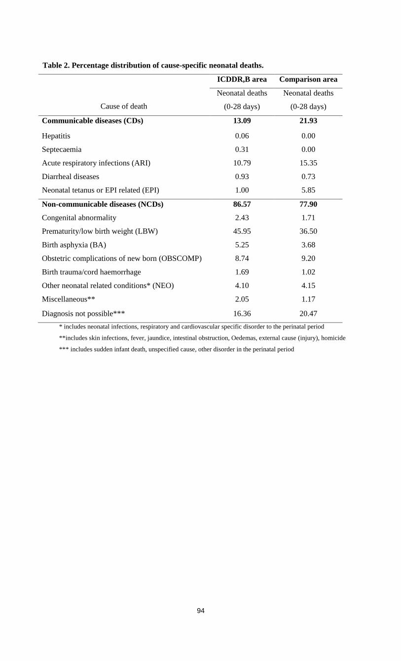
94
Table 2. Percentage distribution of cause-specific neonatal deaths.
Cause of death
ICDDR,B area Comparison area
Neonatal deaths
(0-28 days)
Neonatal deaths
(0-28 days)
Communicable diseases (CDs) 13.09 21.93
Hepatitis 0.06 0.00
Septecaemia 0.31 0.00
Acute respiratory infections (ARI) 10.79 15.35
Diarrheal diseases 0.93 0.73
Neonatal tetanus or EPI related (EPI) 1.00 5.85
Non-communicable diseases (NCDs) 86.57 77.90
Congenital abnormality 2.43 1.71
Prematurity/low birth weight (LBW) 45.95 36.50
Birth asphyxia (BA) 5.25 3.68
Obstetric complications of new born (OBSCOMP) 8.74 9.20
Birth trauma/cord haemorrhage 1.69 1.02
Other neonatal related conditions* (NEO) 4.10 4.15
Miscellaneous** 2.05 1.17
Diagnosis not possible*** 16.36 20.47
* includes neonatal infections, respiratory and cardiovascular specific disorder to the perinatal period
**includes skin infections, fever, jaundice, intestinal obstruction, Oedemas, external cause (injury), homicide
*** includes sudden infant death, unspecified cause, other disorder in the perinatal period
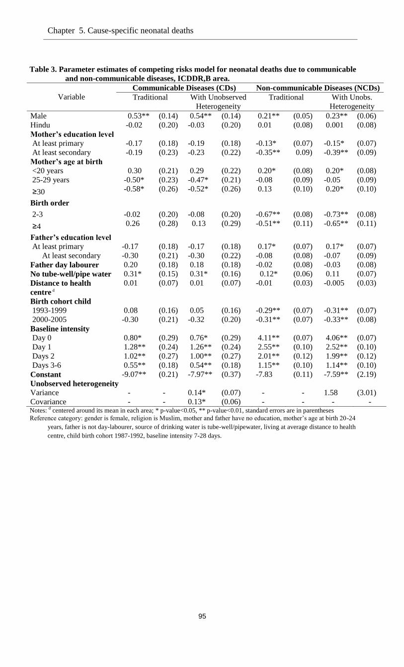
Chapter 5. Cause-specific neonatal deaths
95
Table 3. Parameter estimates of competing risks model for neonatal deaths due to communicable
and non-communicable diseases, ICDDR,B area.
Variable Communicable Diseases (CDs) Non-communicable Diseases (NCDs)
Traditional With Unobserved
Heterogeneity
Traditional With Unobs.
Heterogeneity
Male 0.53** (0.14) 0.54** (0.14) 0.21** (0.05) 0.23** (0.06)
Hindu -0.02 (0.20) -0.03 (0.20) 0.01 (0.08) 0.001 (0.08)
Mother’s education level
At least primary -0.17 (0.18) -0.19 (0.18) -0.13* (0.07) -0.15* (0.07)
At least secondary -0.19 (0.23) -0.23 (0.22) -0.35** 0.09) -0.39** (0.09)
Mother’s age at birth
<20 years 0.30 (0.21) 0.29 (0.22) 0.20* (0.08) 0.20* (0.08)
25-29 years -0.50* (0.23) -0.47* (0.21) -0.08 (0.09) -0.05 (0.09)
≥30 -0.58* (0.26) -0.52* (0.26) 0.13 (0.10) 0.20* (0.10)
Birth order
2-3 -0.02 (0.20) -0.08 (0.20) -0.67** (0.08) -0.73** (0.08)
≥4 0.26 (0.28) 0.13 (0.29) -0.51** (0.11) -0.65** (0.11)
Father’s education level
At least primary -0.17 (0.18) -0.17 (0.18) 0.17* (0.07) 0.17* (0.07)
At least secondary -0.30 (0.21) -0.30 (0.22) -0.08 (0.08) -0.07 (0.09)
Father day labourer 0.20 (0.18) 0.18 (0.18) -0.02 (0.08) -0.03 (0.08)
No tube-well/pipe water 0.31* (0.15) 0.31* (0.16) 0.12* (0.06) 0.11 (0.07)
Distance to health
centre d 0.01 (0.07) 0.01 (0.07) -0.01 (0.03) -0.005 (0.03)
Birth cohort child
1993-1999 0.08 (0.16) 0.05 (0.16) -0.29** (0.07) -0.31** (0.07)
2000-2005 -0.30 (0.21) -0.32 (0.20) -0.31** (0.07) -0.33** (0.08)
Baseline intensity
Day 0 0.80* (0.29) 0.76* (0.29) 4.11** (0.07) 4.06** (0.07)
Day 1 1.28** (0.24) 1.26** (0.24) 2.55** (0.10) 2.52** (0.10)
Days 2 1.02** (0.27) 1.00** (0.27) 2.01** (0.12) 1.99** (0.12)
Days 3-6 0.55** (0.18) 0.54** (0.18) 1.15** (0.10) 1.14** (0.10)
Constant -9.07** (0.21) -7.97** (0.37) -7.83 (0.11) -7.59** (2.19)
Unobserved heterogeneity
Variance - - 0.14* (0.07) - - 1.58 (3.01)
Covariance - - 0.13* (0.06) - - - - Notes:
d centered around its mean in each area; * p-value<0.05, ** p-value<0.01, standard errors are in parentheses
Reference category: gender is female, religion is Muslim, mother and father have no education, mother’s age at birth 20-24
years, father is not day-labourer, source of drinking water is tube-well/pipewater, living at average distance to health
centre, child birth cohort 1987-1992, baseline intensity 7-28 days.
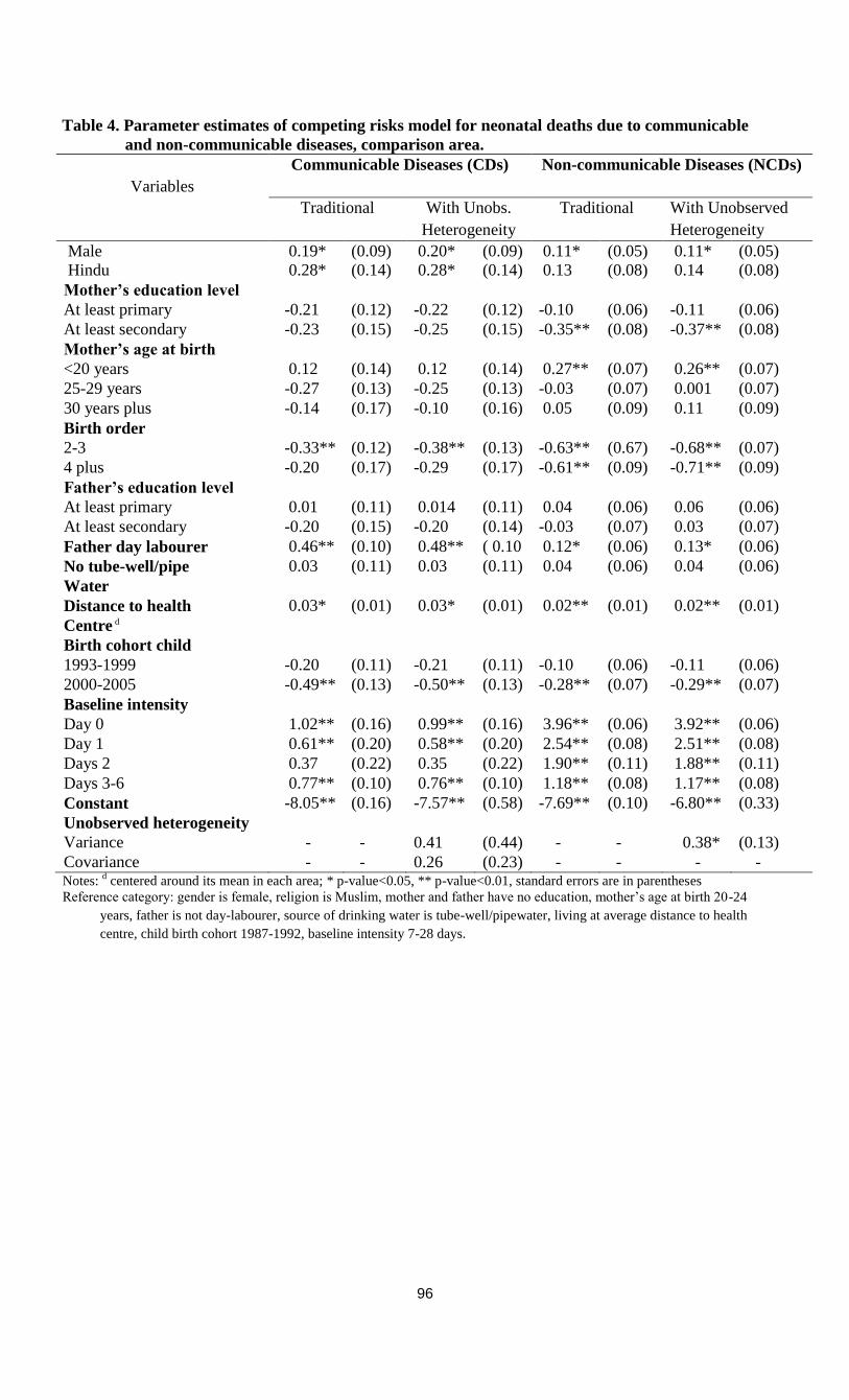
96
Table 4. Parameter estimates of competing risks model for neonatal deaths due to communicable
and non-communicable diseases, comparison area.
Variables
Communicable Diseases (CDs) Non-communicable Diseases (NCDs)
Traditional With Unobs.
Heterogeneity
Traditional With Unobserved
Heterogeneity
Male 0.19* (0.09) 0.20* (0.09) 0.11* (0.05) 0.11* (0.05)
Hindu 0.28* (0.14) 0.28* (0.14) 0.13 (0.08) 0.14 (0.08)
Mother’s education level
At least primary -0.21 (0.12) -0.22 (0.12) -0.10 (0.06) -0.11 (0.06)
At least secondary -0.23 (0.15) -0.25 (0.15) -0.35** (0.08) -0.37** (0.08)
Mother’s age at birth
<20 years 0.12 (0.14) 0.12 (0.14) 0.27** (0.07) 0.26** (0.07)
25-29 years -0.27 (0.13) -0.25 (0.13) -0.03 (0.07) 0.001 (0.07)
30 years plus -0.14 (0.17) -0.10 (0.16) 0.05 (0.09) 0.11 (0.09)
Birth order
2-3 -0.33** (0.12) -0.38** (0.13) -0.63** (0.67) -0.68** (0.07)
4 plus -0.20 (0.17) -0.29 (0.17) -0.61** (0.09) -0.71** (0.09)
Father’s education level
At least primary 0.01 (0.11) 0.014 (0.11) 0.04 (0.06) 0.06 (0.06)
At least secondary -0.20 (0.15) -0.20 (0.14) -0.03 (0.07) 0.03 (0.07)
Father day labourer 0.46** (0.10) 0.48** ( 0.10
)
0.12* (0.06) 0.13* (0.06)
No tube-well/pipe 0.03 (0.11) 0.03 (0.11) 0.04 (0.06) 0.04 (0.06)
Water
Distance to health 0.03* (0.01) 0.03* (0.01) 0.02** (0.01) 0.02** (0.01)
Centre d
Birth cohort child
1993-1999 -0.20 (0.11) -0.21 (0.11) -0.10 (0.06) -0.11 (0.06)
2000-2005 -0.49** (0.13) -0.50** (0.13) -0.28** (0.07) -0.29** (0.07)
Baseline intensity
Day 0 1.02** (0.16) 0.99** (0.16) 3.96** (0.06) 3.92** (0.06)
Day 1 0.61** (0.20) 0.58** (0.20) 2.54** (0.08) 2.51** (0.08)
Days 2 0.37 (0.22) 0.35 (0.22) 1.90** (0.11) 1.88** (0.11)
Days 3-6 0.77** (0.10) 0.76** (0.10) 1.18** (0.08) 1.17** (0.08)
Constant -8.05** (0.16) -7.57** (0.58) -7.69** (0.10) -6.80** (0.33)
Unobserved heterogeneity
Variance - - 0.41 (0.44) - - 0.38* (0.13)
Covariance - - 0.26 (0.23) - - - - Notes:
d centered around its mean in each area; * p-value<0.05, ** p-value<0.01, standard errors are in parentheses
Reference category: gender is female, religion is Muslim, mother and father have no education, mother’s age at birth 20-24
years, father is not day-labourer, source of drinking water is tube-well/pipewater, living at average distance to health
centre, child birth cohort 1987-1992, baseline intensity 7-28 days.
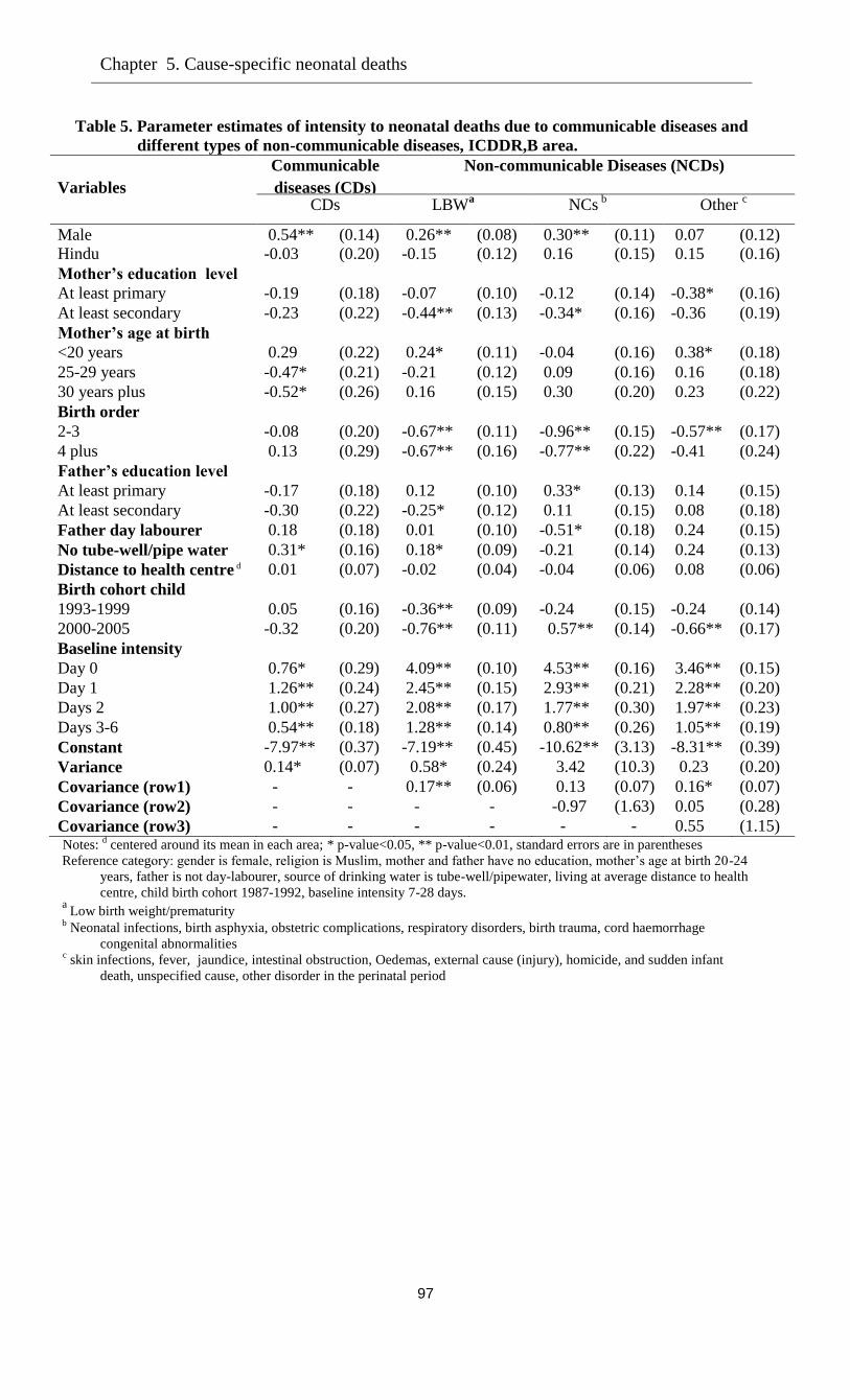
Chapter 5. Cause-specific neonatal deaths
97
Table 5. Parameter estimates of intensity to neonatal deaths due to communicable diseases and
different types of non-communicable diseases, ICDDR,B area.
Variables
Communicable
diseases (CDs)
Non-communicable Diseases (NCDs)
CDs
LBWa NCs
b
Other c
Male 0.54** (0.14) 0.26** (0.08) 0.30** (0.11) 0.07 (0.12)
Hindu -0.03 (0.20) -0.15 (0.12) 0.16 (0.15) 0.15 (0.16)
Mother’s education level
At least primary -0.19 (0.18) -0.07 (0.10) -0.12 (0.14) -0.38* (0.16)
At least secondary -0.23 (0.22) -0.44** (0.13) -0.34* (0.16) -0.36 (0.19)
Mother’s age at birth
<20 years 0.29 (0.22) 0.24* (0.11) -0.04 (0.16) 0.38* (0.18)
25-29 years -0.47* (0.21) -0.21 (0.12) 0.09 (0.16) 0.16 (0.18)
30 years plus -0.52* (0.26) 0.16 (0.15) 0.30 (0.20) 0.23 (0.22)
Birth order
2-3 -0.08 (0.20) -0.67** (0.11) -0.96** (0.15) -0.57** (0.17)
4 plus 0.13 (0.29) -0.67** (0.16) -0.77** (0.22) -0.41 (0.24)
Father’s education level
At least primary -0.17 (0.18) 0.12 (0.10) 0.33* (0.13) 0.14 (0.15)
At least secondary -0.30 (0.22) -0.25* (0.12) 0.11 (0.15) 0.08 (0.18)
Father day labourer 0.18 (0.18) 0.01 (0.10) -0.51* (0.18) 0.24 (0.15)
No tube-well/pipe water 0.31* (0.16) 0.18* (0.09) -0.21 (0.14) 0.24 (0.13)
Distance to health centre d 0.01 (0.07) -0.02 (0.04) -0.04 (0.06) 0.08 (0.06)
Birth cohort child
1993-1999 0.05 (0.16) -0.36** (0.09) -0.24 (0.15) -0.24 (0.14)
2000-2005 -0.32 (0.20) -0.76** (0.11) 0.57** (0.14) -0.66** (0.17)
Baseline intensity
Day 0 0.76* (0.29) 4.09** (0.10) 4.53** (0.16) 3.46** (0.15)
Day 1 1.26** (0.24) 2.45** (0.15) 2.93** (0.21) 2.28** (0.20)
Days 2 1.00**
*
(0.27) 2.08** (0.17) 1.77** (0.30) 1.97** (0.23)
Days 3-6 0.54** (0.18) 1.28** (0.14) 0.80** (0.26) 1.05** (0.19)
Constant -7.97** (0.37) -7.19** (0.45) -10.62** (3.13) -8.31** (0.39)
Variance 0.14* (0.07) 0.58* (0.24) 3.42 (10.3) 0.23 (0.20)
Covariance (row1) - - 0.17** (0.06) 0.13 (0.07) 0.16* (0.07)
Covariance (row2) - - - - -0.97 (1.63) 0.05 (0.28)
Covariance (row3) - - - - - - 0.55 (1.15) Notes:
d centered around its mean in each area; * p-value<0.05, ** p-value<0.01, standard errors are in parentheses
Reference category: gender is female, religion is Muslim, mother and father have no education, mother’s age at birth 20-24
years, father is not day-labourer, source of drinking water is tube-well/pipewater, living at average distance to health
centre, child birth cohort 1987-1992, baseline intensity 7-28 days. a
Low birth weight/prematurity b Neonatal infections, birth asphyxia, obstetric complications, respiratory disorders, birth trauma, cord haemorrhage
congenital abnormalities c skin infections, fever, jaundice, intestinal obstruction, Oedemas, external cause (injury), homicide, and sudden infant
death, unspecified cause, other disorder in the perinatal period
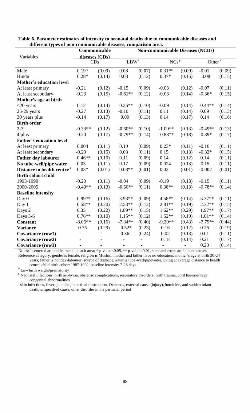
98
Table 6. Parameter estimates of intensity to neonatal deaths due to communicable diseases and
different types of non-communicable diseases, comparison area.
Variables
Communicable
diseases (CDs)
Non-communicable Diseases (NCDs)
CDs
LBWa NCs b Other
c
Male 0.19* (0.09) 0.08 (0.07) 0.31** (0.09) -0.01 (0.09)
Hindu 0.28* (0.14) 0.03 (0.12) 0.37* (0.15) 0.08 (0.15)
Mother’s education level
At least primary -0.21 (0.12) -0.15 (0.09) -0.03 (0.12) -0.07 (0.11)
At least secondary -0.23 (0.15) -0.61** (0.12) -0.03 (0.14) -0.36* (0.15)
Mother’s age at birth
<20 years 0.12 (0.14) 0.36** (0.10) -0.09 (0.14) 0.44** (0.14)
25-29 years -0.27 (0.13) -0.10 (0.11) 0.11 (0.14) 0.09 (0.13)
30 years plus -0.14 (0.17) 0.09 (0.13) 0.14 (0.17) 0.14 (0.16)
Birth order
2-3 -0.33** (0.12) -0.60** (0.10) -1.00** (0.13) -0.49** (0.13)
4 plus -0.20 (0.17) -0.79** (0.14) -0.88** (0.18) -0.39* (0.17)
Father’s education level
At least primary 0.004 (0.11) 0.10 (0.09) 0.23* (0.11) -0.16 (0.11)
At least secondary -0.20 (0.15) 0.03 (0.11) 0.15 (0.13) -0.32* (0.15)
Father day labourer 0.46** (0.10) 0.11 (0.09) 0.14 (0.12) 0.14 (0.11)
No tube-well/pipe water 0.03 (0.11) 0.17 (0.09) 0.024 (0.13) -0.15 (0.11)
Distance to health centre d 0.03* (0.01) 0.03** (0.01) 0.02 (0.01) -0.002 (0.01)
Birth cohort child
1993-1999 -0.20 (0.11) -0.04 (0.09) -0.19 (0.13) -0.15 (0.11)
2000-2005 -0.49** (0.13) -0.50** (0.11) 0.38** (0.13) -0.78** (0.14)
Baseline intensity
Day 0 0.99** (0.16) 3.93** (0.09) 4.58** (0.14) 3.37** (0.11)
Day 1 0.58** (0.20) 2.53** (0.12) 2.81** (0.19) 2.32** (0.15)
Days 2 0.35 (0.22) 1.89** (0.15) 1.62** (0.29) 1.97** (0.17)
Days 3-6 0.76** (0.10) 1.15** (0.12) 1.52** (0.19) 1.01** (0.14)
Constant -8.05** (0.16) -7.34** (0.40) -9.20** (0.43) -7.79** (0.44)
Variance 0.35 (0.29) 0.52* (0.23) 0.16 (0.12) 0.26 (0.19)
Covariance (row1) - - 0.36 (0.24) 0.02 (0.13) 0.01 (0.11)
Covariance (row2) - - - - 0.18 (0.14) 0.21 (0.17)
Covariance (row3) - - - - - - 0.20 (0.14) Notes:
d centered around its mean in each area; * p-value<0.05, ** p-value<0.01, standard errors are in parentheses
Reference category: gender is female, religion is Muslim, mother and father have no education, mother’s age at birth 20-24
years, father is not day-labourer, source of drinking water is tube-well/pipewater, living at average distance to health
centre, child birth cohort 1987-1992, baseline intensity 7-28 days. a
Low birth weight/prematurity b Neonatal infections, birth asphyxia, obstetric complications, respiratory disorders, birth trauma, cord haemorrhage
congenital abnormalities c skin infections, fever, jaundice, intestinal obstruction, Oedemas, external cause (injury), homicide, and sudden infant
death, unspecified cause, other disorder in the perinatal period
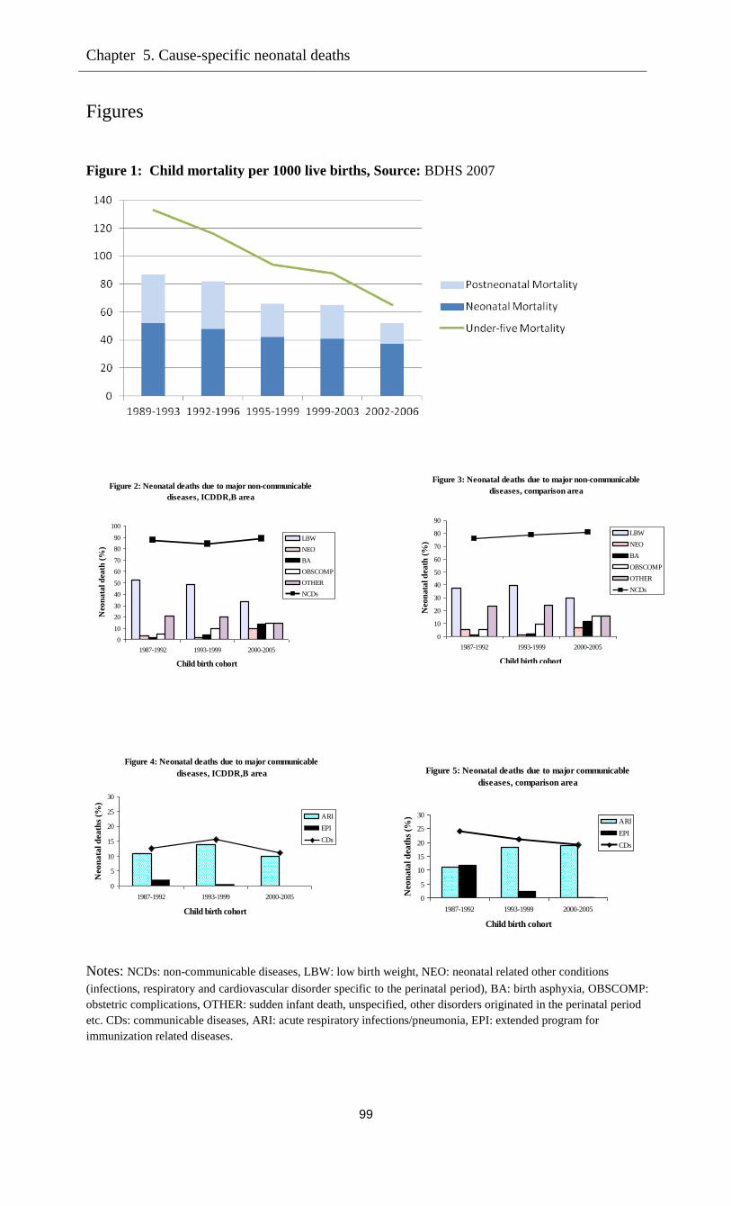
Chapter 5. Cause-specific neonatal deaths
99
Figures
Figure 1: Child mortality per 1000 live births, Source: BDHS 2007
Figure 2: Neonatal deaths due to major non-communicable
diseases, ICDDR,B area
0
10
20
30
40
50
60
70
80
90
100
1987-1992 1993-1999 2000-2005
Child birth cohort
Neo
na
tal d
eath
(%
)
LBW
NEO
BA
OBSCOMP
OTHER
NCDs
Figure 4: Neonatal deaths due to major communicable
diseases, ICDDR,B area
0
5
10
15
20
25
30
1987-1992 1993-1999 2000-2005
Child birth cohort
Neo
na
tal d
ea
ths
(%)
ARI
EPI
CDs
Notes: NCDs: non-communicable diseases, LBW: low birth weight, NEO: neonatal related other conditions
(infections, respiratory and cardiovascular disorder specific to the perinatal period), BA: birth asphyxia, OBSCOMP:
obstetric complications, OTHER: sudden infant death, unspecified, other disorders originated in the perinatal period
etc. CDs: communicable diseases, ARI: acute respiratory infections/pneumonia, EPI: extended program for
immunization related diseases.
Figure 3: Neonatal deaths due to major non-communicable
diseases, comparison area
0
10
20
30
40
50
60
70
80
90
1987-1992 1993-1999 2000-2005
Child birth cohort
Neo
nata
l d
eath
(%
)
LBW
NEO
BA
OBSCOMP
OTHER
NCDs
Figure 5: Neonatal deaths due to major communicable
diseases, comparison area
0
5
10
15
20
25
30
1987-1992 1993-1999 2000-2005
Child birth cohort
Neo
na
tal d
eath
s (%
)
ARI
EPI
CDs
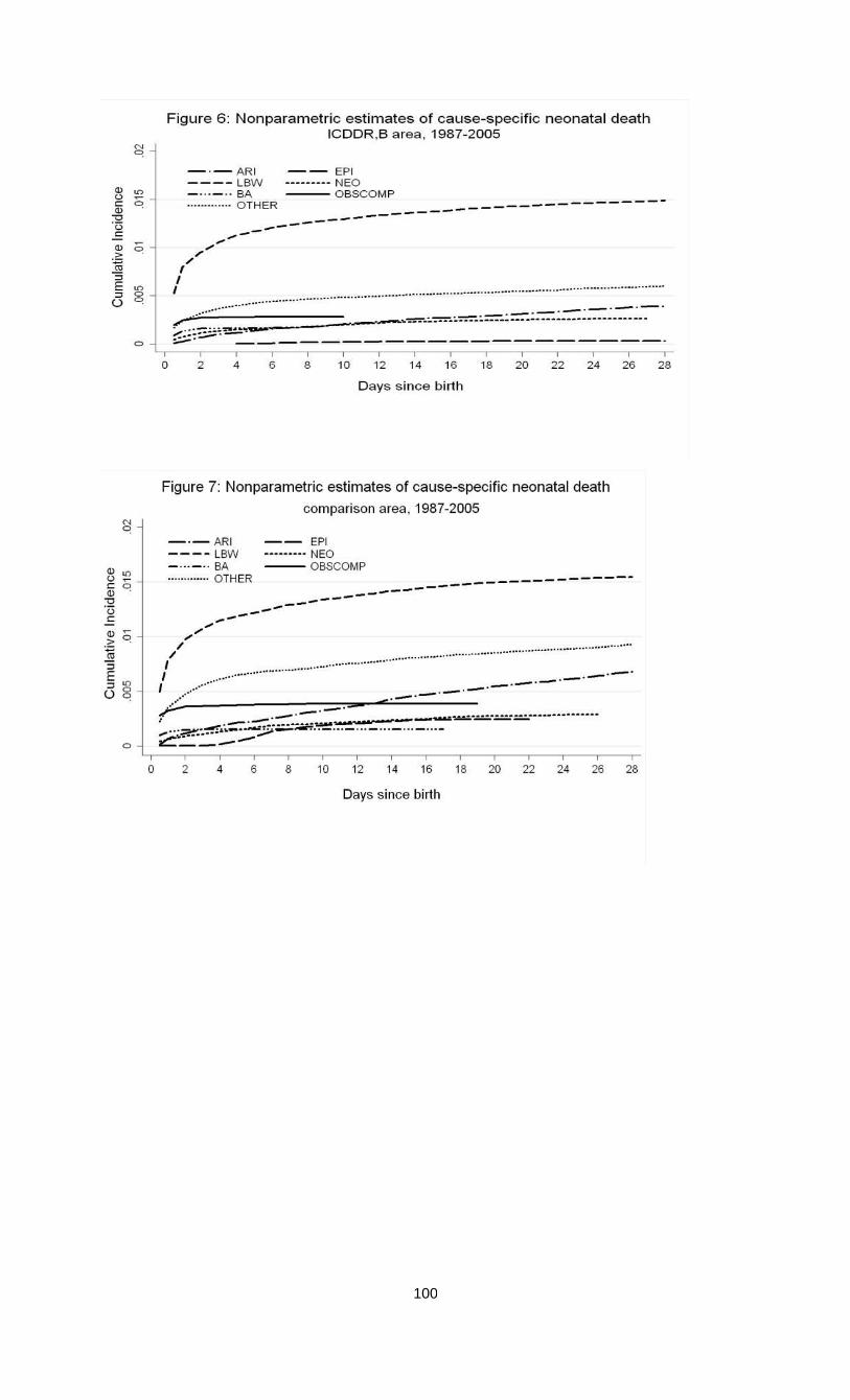
100
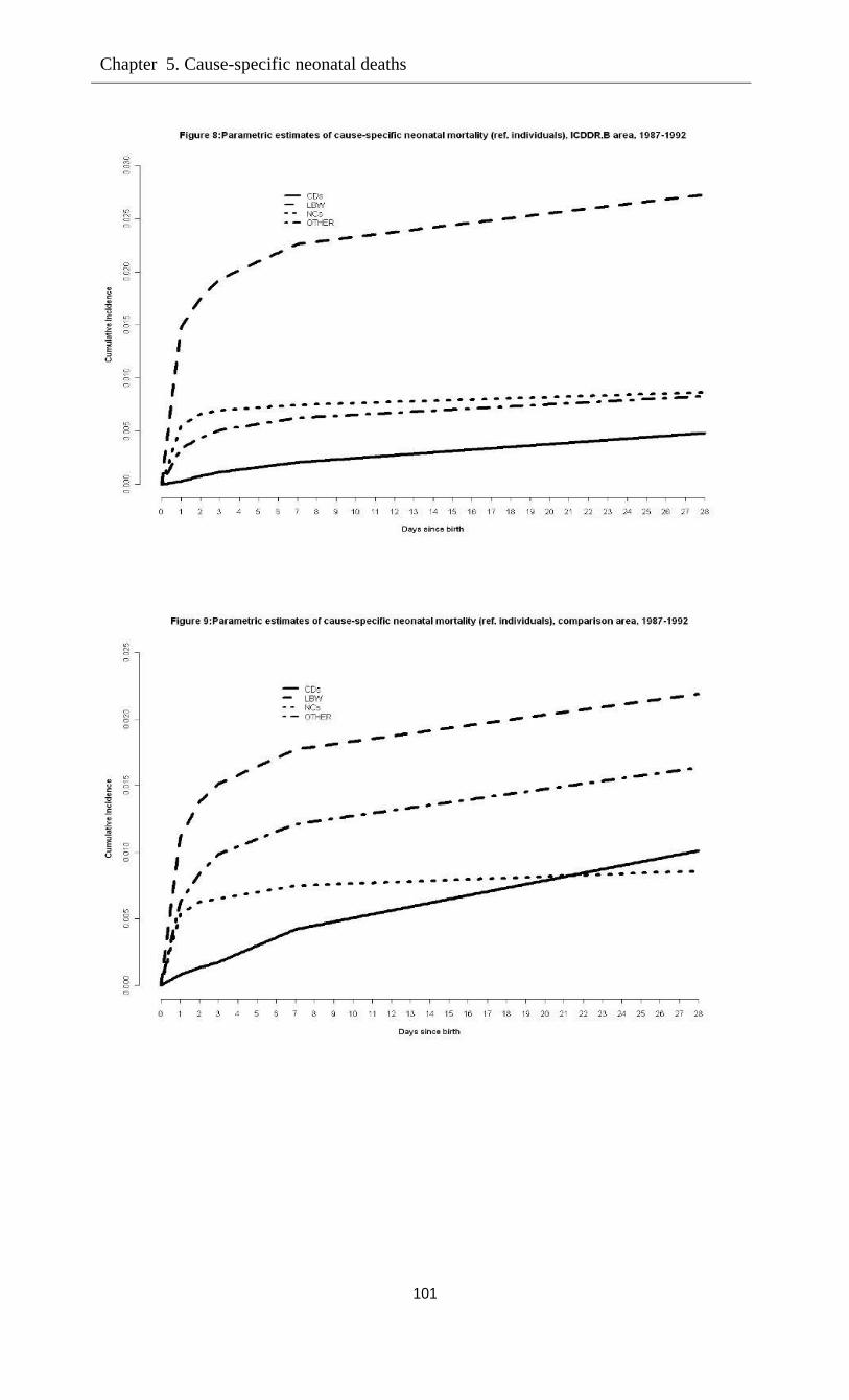
Chapter 5. Cause-specific neonatal deaths
101
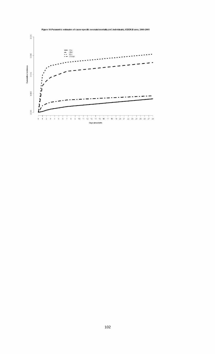
102

Chapter 5. Cause-specific neonatal deaths
103
Annex
Table A1: Assignment of causes of neonatal death, 1987-2005, HDSS, Matlab, Bangladesh.
Codes (ICD9, ICD10)
Labels of code
Categories used (Table 2)
Categories used
(Table 5 & 6)
190, 192, 193,452,458,P05,P07 Preterm delivery/low birth
weight
Low birth weight (LBW) LBW
454,P21 Birth asphyxia Birth asphyxia (BA)
NCs
457, 456, P22-P29, P35,P36,P51,P76,P80 infections, respiratory and
cardiovascular disorder specific
to the perinatal period
Neonatal related conditions
(NEO)
449, Q01, Q02, Q03,Q24, Q35,Q37,
Q42,Q45,Q89
Congenital abnormalities Congenital abnormalities
(CA)
453, P15 Birth trauma Birth trauma
451,P00,P01,P02,P03 Obstetric complications OBSCOMP
P59 Haemorragic Haemorragic
P90-P96 Other disorders originated in
the perinatal period
unspecified
OTHER
990,998,999,R34,R95,R96,R99 Unspecified causes
R95,450,459 Sudden death
K75, W75,X91,
293,344,420,460,461,552,555,559,691,738
,
Other specific Other specific
010,013,014 Acute watery diarrhoea,
dysentery, acute non-watery
diarrhoea
Diarrhoea, dysentery
CDs
038, 046 Septicamia, viral hepatitis Septicemia, hepatitis
321, 325,328,191 Pneumonia, ALRI, Pneumonia
with diarrhoea, Pneumonia
severe
ARI
A41,B01,G03,J11,J18, A03 Other bacterial diseases, viral
infections characterized by skin
and mucous membrane lesions
ARI
456 EPI EPI

Chapter 6
Summary and conclusion
Child mortality in Bangladesh remains an important issue. Under-five mortality declined sharply
during the last decades of the previous century, but the reduction is levelling off and child
mortality is not declining fast enough to meet the Millennium Development Goal 4 of reducing
under-five mortality by two-thirds between 1990 and 2015 (see United Nations 2001), so the
further reduction of child mortality remains a significant challenge. Several hypotheses
concerning possible causal mechanisms that increase or reduce child mortality were tested in the
four papers included in the thesis.
The second chapter analysed infant mortality in Bangladesh, focusing on explaining death
clustering within families, using prospective data from Matlab, Bangladesh, split into areas with
and without extensive health services (the area covered by the International Centre for
Diarrhoeal Disease Research: ICDDR,B and the comparison area, respectively). The modelling
framework distinguished between two explanations of death clustering: (observed and
unobserved) heterogeneity across families and a causal 'scarring' effect of the death of one infant
on the survival chances of the next to be born. Keeping observed and unobserved characteristics
constant, scarring was observed in the comparison area only. There the likelihood of infant death
is about 29 per cent greater if the previous sibling died in infancy than otherwise. This effect
mainly works through birth intervals: infant deaths are followed by shorter birth intervals, which
increases the risk of infant death for the next child.
In the third chapter, using the same data sets as in first paper, we jointly analyzed infant
mortality, birth spacing, and the probability of having another birth. To distinguish causal
mechanisms from unobserved heterogeneity and reverse causality, this paper exploited dynamic
panel data techniques, building on recent work by Bhalotra and van Soest (2008). The results are
comparable between a treatment area with extensive health services and a comparison area with
the standard health services provided by the government.
The results demonstrate that death at infancy of the previous child shortens the
subsequent length of birth space by 49% in the ICDDR,B area and 46% in comparison area. As a
result of replacement, every infant death in the comparison area leads to 0.54 births on average
(and 0.51 births survive the first 12 months). In the ICDDR,B area, each infant death leads to
0.42 replacement births. The effects of the numbers of (surviving) boys and girls are consistent
with son preference: having more surviving boys has a stronger positive effect on the birth
interval than having more girls, though both effects are significant. Not having any surviving
boys or girls leads to the shortest birth interval. Simulations on the basis of the estimated models

105
show how fertility and mortality can be reduced by, for example, breaking the causal link that
leads to a short interval after a child has died.
In the fourth chapter, we investigated the causal role of contraceptive use on birth spacing
and thereby on infant mortality. Using the same data set on the ICDDR,B area (since information
on contraceptives is only available in that area), this paper extends the modelling framework
used in the third chapter. The analysis is based on a three-part model: an equation explaining
infant mortality, a model explaining whether contraceptives are used after a child is born (and if
so, for how long), and an equation explaining birth intervals. Infant mortality is determined by
covariates reflecting socio-economic status and other background characteristics, but also by the
length of the preceding birth interval. Decisions about contraceptives are driven by similar
covariates, but also by the survival status of the previous child and the family’s gender
composition. Birth spacing is driven by contraceptive use and other factors. Each part of the
model incorporates unobserved mother specific heterogeneity. Results confirm the favourable
effects of family planning programmes on child survival for second and higher birth orders that
work through birth spacing. Our results imply that if family planning programmes would be
expanded so that everyone would use contraceptives after each birth, a 7.9% reduction in infant
mortality could be achieved – a reduction of 11 infant deaths per 1000 live births. This leads to
the policy implication that strengthening family planning programs helps to reduce infant
mortality.
The fifth chapter reports the underlying epidemiology of neonatal child deaths, taking
into account the competing risks of neonatal deaths. A competing risk duration model is used
incorporating both observed and unobserved mother specific heterogeneity, and assuming
heterogeneity terms across various causes can be correlated. The results confirm the general
conclusion on levels, trends and patterns of causes of neonatal deaths in the existing literature,
but also reveal some remarkable socioeconomic differences in the risks of cause-specific deaths.
Deaths due to low birth weight and other causes (sudden infant death, unspecified or specified)
are better explained by the socio-economic covariates than deaths due to neonatal infections or
obstetric complications.
The analysis in this thesis highlights the role of maternal and child health interventions
(particularly tetanus toxoid immunization for pregnant women, nutrition programs, and high
coverage health services / reduced distance to the nearest health centre). Policies that increase
quality and equity in births may help to further reduce neonatal mortality.

106
Bibliography
Adjuik, M., Smith, T., Clark, S., Todd, J., Garrib, A., Kinfu, Y., Kahn, K., Mola, M., Ashraf, A.,
Masanja, H., Adazu, U., Sacarlal, J,, Alam, N., Maria, A., Gbangou, A., Mwageni, E., &
Binka, F. (2006). Cause-specific mortality rates in sub-Saharan Africa and Bangladesh.
Bulletin of World Health Organization, 84: 181-188.
Alam, N. (1995). Birth spacing and infant and early childhood mortality in a high fertility area of
Bangladesh: Age–dependent and interactive effects. Journal of Biosocial Science, 27: 393-
404.
Alam, N. & David, P.H. (1998). Infant and child mortality in Bangladesh: Age-specific effects of
previous child’s death. Journal of Biosocial Science, 30: 333-348.
Anwar, I., Killewo, J., Chowdhury, M.E., & Dasgupta, S.K. (2004). Bangladesh: Inequalities in
utilization of maternal health care services – Evidence from Matlab. Discussion paper,
Number 2, Dhaka: Health, Nutrition and Population.
Arulampalam, W. & Bhalotra, S. (2006). Sibling death clustering in India: State dependence
versus unobserved heterogeneity. Journal of the Royal Statistical Society A, 169: 829-848.
Arulampalam, W. & Bhalotra, S. (2008). The linked survival prospects of siblings: Evidence
from the Indian states. Population Studies, 62: 171-190.
Arulampalam, W. & Stewart, M.B. (2009). Simplified implementation of the heckman estimator
of the dynamic probit model and a comparison with alternative estimators. Oxford Bulletin of
Economics and Statistics, 71: 659-681.
Bairagi, R., Sutradhar, S.C., & Alam, N. (1999). Levels, trends and determinants of child
mortality in Matlab, Bangladesh, 1966–1994. Asia-Pacific Population Journal, 14: 51–68.
Bairagi, R., Islam, M.M., & Barua, M.K. (2000). Contraceptive failure: Levels, trends and
determinants in Matlab, Bangladesh. Journal of Biosocial Science, 32: 107-123.
Bang, A.T., Bang, R.A., Baitule, R.B., Reddy, H.M., & Deshmukh, M.D. (2005). Management
of birth asphyxia in home deliveries in rural Gadchiroli: The effect of two types of birth
attendants and of resuscitating with mouth-to-mouth, tube-mask or bag-mask. Journal of
Perinatology, 25(Suppl): S82-S91.
Bari, W., Chowdhury, R.I., Islam, M.A., Chakraborty, N., & Akhter, H.A. (2002). The
differentials and determinants of perinatal mortality in rural Bangladesh. European Journal of
Contraception and Reproductive Health Care, 7: 216-222.
Baqui, A.H., Sabir. A.A., Begum. N., Arifeen. S.E., Mitra. S.N., & Black, R.E. (2001). Causes of
childhood deaths in Bangladesh: An update. Acta Paediatrica, 90: 682-690.
Ben-Porath, Y. (1976). Fertility response to child mortality: Micro data from Israel. The Journal
of Political Economy, l84: S163-S178.
Bhalotra, S. & van Soest, A. (2008). Birth spacing, fertility and neonatal mortality in India:
Dynamics, frailty and fecundity. Journal of Econometrics, 143: 274-290.
Bhalotra, S., Valente, C., & van Soest, A. (2010a). Religion and childhood death in India. In:
Basant, R. and Sharif, A. (eds.). Handbook of Muslims in India. Delhi: Oxford University
Press: 123-165.
Bhalotra, S., Valente, C., & van Soest, A. (2010b). The puzzle of Muslim
advantage in child survival in India. Journal of Health Economics, 29: 191-204.

107
Bhatia, S. (1981). Traditional childbirth practices: Implications for a rural MCH program.
Studies in Family Planning, 12: 66-75.
Bhatia, S. (1983). Contraceptive users in rural Bangladesh - a time trend analysis. Studies in
Family Planning, 14: 20-28.
Bhatia, S. (1989). Patterns and causes of neonatal and postneonatal mortality in rural Bangladesh.
Studies in Family Planning, 20: 136-146.
Bhuiya, A., Zimicki, S., & D`Souza, S. (1986). Socioeconomic differentials in child nutrition and
morbidity in a rural area of Bangladesh. Journal of Tropical Pediatrics, 32: 17-23.
Blinder, A. S. (1973). Wage discrimination: Reduced form and structural estimates.
Journal of Human Resources, 8: 436–455.
Bolstad, W. M. & Manda, S.O. (2001). Investigating child mortality in Malawi using family and
community random effects: A bayesian analysis. Journal of the American Statistical
Association, 96: 12-19.
Bongaarts, J. (1987). Does family planning reduce infant mortality? Comment. Population and
Development Review, 13: 323-334.
Bryce, J., Cynthia, B.P., Shibuya, K., & Black, R.E. (2005). WHO child health epidemiology
reference group, WHO estimates of the causes of death in children. Lancet, 365: 1147-1152.
Butler, J. S. & Moffitt, R. (1982). A computationally efficient quadrature procedure for the one-
factor multinomial probit model. Econometrica, 50: 761-764.
Caldwell, J.C. (1993). Health transition: The cultural, social and behavioural determinants of
health in the Third World. Social Science & Medicine, 36: 125-135.
Caldwell, J.C. & Caldwell, P. (1978). The achieved small family: Early fertility transition in an
African city. Studies in Family Planning, 9: 2-18.
Caldwell, J.C., Findley, S., Caldwell, P., Santow, G., Cosford, W., Braid, J., & Broers-Freeman,
D. (eds). (1990). What we know about health transition: The cultural, social and behavioural
determinants of health. Volumes 2, Canberra: Australian National University.
Chen, L.C., Rahman, M., & Sarder, A.M. (1980). Epidemiology and causes of death among
children in a rural area of Bangladesh. International Journal of Epidemiology, 9: 25-33.
Chowdhury, A.K.M., Khan, A.R. & Chen, L. (1976). The effect of child mortality experience on
subsequent fertility: In Pakistan and Bangladesh. Population Studies, 30: 263-278.
Chowdhury, H.R., Thompson, S., Ali, M., Alam, N., Yunus, M., & Streatfield, P.K. (2010).
Causes of neonatal deaths in a rural subdistrict of Bangladesh: Implications for intervention.
Journal of Health Population Nutrition, 28: 375-382.
Chowdhury, M.K. & Bairagi, R. (1990). Son preference and fertility in Bangladesh. Population
and Development Review, 16: 749-757.
Cleland, J. & Sathar, Z.A. (1984). The effect of birth spacing on childhood mortality in Pakistan.
Population Studies, 38: 401-418.
Conde-Agudelo, A.,Belizan, J.M., & Diaz-Rossello, J. (2003). Kangaroo mother care to reduce
morbidity and mortality in low birth weight infants (Cochrane Review). In: The Cochrane
Library. Issue 4, Oxford: Update Software.
Conde-Agudelo, A., Rosas-Bermudez, A., & Kafury-Goeta, A.C. (2006). Birth spacing and risk
of adverse perinatal outcomes: a meta-analysis. Journal of the American Medical Association,
295: 1809-1823.
108
Cornfield, J. (1957). The estimation of the probability of developing a disease in the presence of
competing risks. Disease Probability, 47: 601-607.
Coviello, V. & Boggess, M. (2004). Cumulative incidence estimation in the presence of
competing risks. The Stata Journal, 4: 103-112.
Cox, D.R. (1959). The analysis of exponentially distributed life-times with two types of failures.
Journal of the Royal Statistical Society B, 21: 411-421.
Curtis, S.L., Diamond, I. & McDonald, J.W. (1993). Birth interval and family effects on
postneonatal mortality in Brazil. Demography, 30: 33-43.
DasGupta, M. (1990). Death clustering, mothers’ education and the determinants of child
mortality in rural Punjab. India Population Studies, 44: 489-505.
Datta, A.K., & Bairagi, R. (2000). Improvement in female survival: A quite revolution in
Bangladesh. Asia Pacific Population Journal, 15: 19-40.
DaVanzo, J. & Starbird, E.H. (1991). Correlates of short interbirth intervals in Peninsular
Malaysia: Their pathways of influence through breastfeeding and contraceptive use. Studies in
Family Planning, 22: 241-254.
DaVanzo, J. & Pebley, A.R. (1993). Maternal depletion and child survival in Guatemala and
Malayasia. Santa Monica: Rand Corporation.
DaVanzo, J., Razzaque, A., Rahman, M., & Hale, L. (2004). The effects of birth spacing on
infant and child mortality, pregnancy outcomes, and maternal morbidity and mortality in
Matlab, Bangladesh. Santa Monica: Rand Corporation.
DaVanzo, J., Hale, L., Razzaque, A., & Rahman, M. (2007). Effects of interpregnancy interval
and outcome of the preceding pregnancy on pregnancy outcomes in Matlab, Bangladesh.
British Journal of Obstetrics and Gynaecology, 114: 1079-1087.
DaVanzo, J., Hale, L., Razzaque, A., & Rahman, M. (2008). The effects of pregnancy spacing on
infant and child mortality in Matlab, Bangladesh: How they vary by the type of pregnancy
outcome that began the interval. Population Studies, 62: 131-154.
D’Souza, S. (1981). A population laboratory for studying disease processes and mortality- the
demographic surveillance system, Matlab Comilla, Bangladesh. Rural Demography, 8: 29-51.
D’Souza, S. and A. Bhuiya. (1982). Socioeconomic mortality differentials in a rural area of
Bangladesh. Population and Development Review, 8: 753-769.
Fairlie, R.W. (2005). An Extension of the blinder-oaxaca decomposition technique to logit and
probit models. Journal of Economic and Social Measurement, 30: 305-316.
Fauveau, V., Koenig, M.A., & Wojtyniak, B. (1991). Excess female deaths among rural
Bangladeshi children: An examination of cause-specific mortality and morbidity.
International Journal of Epidemiology, 20: 729-735.
Fauveau, V., Wojtyniak, B., Chowdhury, H.R.,& Sarder, A.M. (1994). Assessment of cause of
death in the Matlab Demographic Surveillance System. In: Fauveau V (eds.). Matlab:
Women, Children and Health. Dhaka: International Centre for Diarrhoeal Diseases Research:
65-86.
Fine, J.P. & Gray, R.J. (1999). A proportional hazards model for the subdistribution of a
competing risk. Journal of the American Statistical Association, 94: 496-509.
Fotouhi, A. R. (2005). The initial condition problem in longitudinal binary process: A simulation
study. Simulation Modelling Practice and Theory, 13: 566-583.

109
Goldberg, I.D., Lovin, M.L., Gerhardt, P.R., Handy, V.H., & Cashman, R.E. (1956). The
probability of developing cancer. Journal of the National Cancer Institute, 17: 155-173.
Gubhaju, B. B. (1985). The effect of previous child death on infant and child mortality in rural
Nepal. Studies in Family Planning, 16: 231-236.
Guo, G. (1993). Use of sibling data to estimate family mortality effects in Guatemala.
Demography, 30: 15-32.
Guo, G. & Rodriguez, G. (1992). Estimating a multivariate proportional hazard model via the
EM algorithm, with an application to child survival in Guatemala. Journal of the American
Statistical Association, 87: 969-976.
Haaga, J. G. (1991). Mechanisms for the association of maternal age, parity, and birth spacing
with infant health. Santa Monica: RAND Corporation.
Hale, L., DaVanzo, J., Razzaque, A., & Rahman, M. (2006). Why are infant and child mortality
rates lower in the MCH-FP area of Matlab, Bangladesh? Studies in Family Planning, 37: 281-
292.
Hale, L., DaVanzo, J., & Razzaque, A. (2009). Which factors explain the decline in infant and
child mortality in Matlab, Bangladesh? Journal of Population Research, 26: 3-20.
Hajivassiliou, V. A., & Ruud, P.A.(1994). Classical estimation methods for LDV models using
simulation. In: Robert F. Engle and Daniel L. McFadden (eds.). Handbook of Econometrics.
Volume IV, Amsterdam: North-Holland: 2384-2438.
Harrington, J.A. (1971). The effect of high infant and childhood mortality on fertility: The west
African case. Concerned Demography, 3: 22-35.
Heckman, J.J. (1981). The incidental parameters problem and the problem of initial conditions in
estimating a discrete time – discrete data stochastic process. In: C.F. Manski and D.,
McFadden (eds.). Structural Analysis of discrete data with econometric applications.
Cambridge: MIT Press: 114-178.
Heckman, J.J., Holtz, J., & Walker, J.R. (1985). New evidence on the timing and spacing of
births. American Economic Review, 75: 179-184.
Hobcraft, J. N., McDonald, J.W., & Rutstein, S.O. (1983). Childspacing effects on infant and
early child mortality. Population Index, 49: 585-618.
Hobcraft, J. N., McDonald, J.W., & Rutstein, S.O. (1985). Demographic determinants of infant
and early child mortality: A comparative analysis. Population Studies, 39: 363-385.
Huffman, S. L., Kathleen, F., Hubert A. A., & Streble, P. (1987). Nutrition and fertility in
Bangladesh: Breastfeeding and post partum amenorrhoea. Population Studies, 41: 447-462.
ICDDR,B Centre for Health and Population Research, Dhaka, Bangladesh. (2006). Health and
Demographic Surveillance System-Matlab: Registration of health and demographic events
2004. Scientific Report 93.
Jones, G, Steketee, R., Black, R., Bhutta, Z., & Morris, S. (2003). How many child deaths can
we prevent this year? Lancet, 362: 65-71.
Karar, Z.A., Alam, N., & Streatfield, P.K. (2009). Epidemiological transition in rural Bangladesh,
1986-2006. Global Health Action, DOI:10.3402/gha.v2i0.1904.
Knodel, J. (1978). European populations in the past: Family-level relations. In: S.H. Preston
(eds.). The effects of infant and child mortality on fertility. New York: Population Division,
United Nations.

110
Koenig, M.A., Phillips, J.F., Campbell, O.M., & D’Souza, S. (1990). Birth intervals and
childhood mortality in rural Bangladesh. Demography, 27: 251-265.
Koenig, M. A., Rob, U., Khan, M.A., Chakraborty, J., & Fauveau, V. (1992). Contraceptive use
in Matlab, Bangladesh in 1990: Levels, trends, and expectations. Studies in Family Planning,
23: 352-364.
Lancaster, T. (1979). Econometric methods for the duration of unemployment. Econometrica, 47:
939-956.
Lawn, J.E., Cousens, S., & Zupan, J. (2005). 4 million neonatal deaths: When? Where? Why?
Lancet, 365: 891-900.
Lawn, J.E., Wilczynska, K., & Cousens, S.N. (2006). Estimating the causes of 4 million neonatal
deaths in the year 2000. International Journal of Epidemiology, 35: 706-718.
LeGrand, T.K. & Phillips, J.F. (1996). The effect of fertility reductions on infant and child
mortality: Evidence from Matlab in rural Bangladesh. Population Studies, 50: 51-68.
Madise, N.J. & Diamond, I. (1995). Determinants of infant mortality in Malawi: An analysis to
control for death clustering within families. Journal of Biosocial Science, 27: 95-106.
Majumder, A. K., May, M., & Pant, P.D. (1997). Infant and child mortality determinants in
Bangladesh: Are they changing? Journal of Biosocial Science, 29: 385-399.
Manton, K.G., Stallard, E., & Vaupel, J. W. (1981). Methods for the mortality experience of
heterogeous populations. Demography, 18: 389-410.
Matthiesson, P.C., & McCann, J.C. (1976). The role of mortality in the European fertility
transition: Aggregate-level relations. In: S.H. Preston (ed.). The effects of infant and child
mortality on fertility. New York: Academic Press: 47-68.
Miller, J.E., Trussell, J., Pebley, R.A., & Vaughan, B. (1992). Birth spacing and child mortality
in Bangladesh and Philippines. Demography, 29: 305-318.
Moffitt, R. (2005). Remarks on the analysis of causal relationships in population research.
Demography, 42: 91-108.
Mondot-Bernard, J.M. (1977). Relationships between fertility, child Mortality and nutrition in
Africa. Tentative analysis. Technical papers, Paris: Development Centre of OECD.
Mosley, W.H. & Chen, L.C. (1984). An analytical framework for the study of child survival in
developing countries. Population Development Review, 10(Suppl.): 25-45.
National Institute of Population Research and Training (NIPORT), Mitra and Associates, and
ORC Macro. (2005). Bangladesh Demographic Health Survey 2004. Dhaka, Bangladesh and
Calverton, Maryland [USA].
National Institute of Population Research and Training (NIPORT), Mitra and Associates, and
ORC Macro. (2008). Bangladesh Demographic Health Survey 2007. Dhaka, Bangladesh and
Calverton, Maryland [USA].
Nyarko, P., Madise, N.J., & Diamond, I. (2003). Child loss and fertility behaviour in Ghana.
Southampton, UK: Social Statistics Research Centre, S3RI Application and Policy Working
Paper, A03/08, p. 25.
Oaxaca, R. (1973). Male-female wage differentials in urban labor markets. International
Economic Review, 14: 693–709.
Omariba, D. W. R., Fernando R., & Roderic, B. (2008). Correlated mortality of siblings in
Kenya: The role of state dependence. Demographic Research, 18: 311-336.
111
Omran, A.R. (1982). Epidemiological transition: Theory. In: Ross J.A. (eds.). International
Encyclopedia of Population. Volume 1, New York: The Free Press: 172-75.
Park, C.B., Islam, M.A., Chakraborty, N., & Kantner, A. (1998). Partitioning the effect of infant
and child death on subsequent fertility: An exploration in Bangladesh. Population Studies, 52:
345-356.
Phillips, J.F., Simmons, R., Chakraborty, J., & Chowdhury, A.I. (1984). Integrating health
services into an MCH-FP program: Lessons from Matlab, Bangladesh. Studies in Family
Planning, 15: 153-161.
Phillips, J.F., Simons, R., Koenig, M.A., & Chakraborty, J. (1988). Determinants of reproductive
change in a traditional society: Evidence from Matlab, Bangladesh. Studies in Family
Planning, 19: 313-334.
Phillips, J. F., Wayne, S. S., Shushum, B., Rahman, M., & Chakraborty, J. (1982). The
demographic impact of the family planning-health services project in Matlab, Bangladesh.
Studies in Family Planning, 13: 131-140.
Potter, J. E. (1988). Does family planning reduce infant mortality? Comment. Population and
Development Review, 14: 179-187.
Pritchett, H.L. (1994). Desired fertility and the impact of population policies. Population and
Development Review, 20: 1-55.
Rahman, M., Akbar, J., Phillips, J.F., & Becker, S. (1992). Contraceptive use in Matlab,
Bangladesh: The role of gender preference. Studies in Family Planning, 23: 229-242.
Rahman, M. & DaVanzo J. (1993). Gender preference and birth spacing in Matlab, Bangladesh.
Demography, 30: 315-332.
Rahman, A., Iqbal, Z., Bunn, J., Lovel, H., & Harrington, R. (2004). Impact of maternal
depression on infant nutritional status and illness: A cohort study. Archives of General
Psychiatry, 61: 946-952.
Razzaque, A., Streatfield, P.K., & Gwatkin, D.R. (2007). Does health intervention improve
socioeconomic inequalities of neonatal, infant and child mortality? Evidence from Matlab,
Bangladesh. International Journal for Equity in Health, 6: 1-7.
Reddiah,V.P. & Kapoor, S.K. (1988). Acute respiratoty infection in rural under-fives. Indian
Journal of Pediatrics, 55: 424-426.
Retherford, R.D., Choe, M.K., Shyam, T., & Gubhaju, B.B. (1989). To what extent does
breastfeeding explain birth-interval effects on early childhood mortality? Demography, 26:
439-450.
Ronsmans, C., Chowdhury, M.E., DasGupta, S.K., Ahmed, A., & Koblinsky, M. (2010). Effect
of parent’s death on child survival in rural Bangladesh: A cohort study. Lancet, 375: 2024-
2030.
Rosenblum, D. (2009). Economic causes of sex discrimination in India, PhD thesis. Yale
University.
Rosenzweig, M.R. & Wolpin, K.I. (1988). Heterogeneity, intrafamily distribution, and child
health. Journal of Human Resources, 23: 437-461.
Rutstein, S. (2005). Effects of preceding birth and pregnancy intervals on child mortality and
nutritional status in less developed countries: Evidence from the demographic and health
surveys. International Journal of Gynecology and Obstetrics, 89: S7-S24.
112
Saha, U.R., Kamal, N., & Bairagi, R. (2004). Discontinuation of contraceptives and method
switching in rural Bangladesh. Sharing Population and Development Research across South
and West Asia. Fifth Annual Research Conference Proceedings, 14-16 December, 2004.
Saha, U.R. & van Soest A. (2011). Infant death clustering in families: Magnitude, causes, and the
influence of better health services, Bangladesh 1982-2005. Population Studies, 65: 273-287.
Santow, G., & Bracher M. D. (1984). Child death and time to the next birth in Central Java.
Population Studies, 38: 241-53.
Sastry, N. (1997). Family-level clustering of childhood mortality risk in Northeast Brazil.
Population Studies, 51: 245-261.
Scrimshaw, N. (1996). Nutrition and health from womb to tomb. Nutrition Today, 31: 55-67.
Smith, D. P. (1985). Breastfeeding, contraception, and birth intervals in developing countries.
Studies in Family Planning, 16: 154-163.
Stange, K. (2011). A longitudinal analysis of the relationship between fertility timing and
schooling. Demography, 48: 931-956.
Steele, F. & Diamond, I. (1999). Contraceptive switching in Bangladesh. Studies in Family
Planning, 30: 315-328.
Steer, R. A., Scholl, T.O., Hediger, M.L., Fischer, R.L. (1992). Self-reported depression and
negative pregnancy outcomes. Journal of Clinical Epidemiology, 45: 1093-1099.
Stewart, M. B. 2007. The interrelated dynamics of unemployment and low-wage employment.
Journal of Applied Econometrics, 22: 511-531.
Sufian, A. J. M., & Johnson, N.E. (1989). Son preference and child replacement in Bangladesh:
A new look at the child survival hypothesis. Journal of Biosocial Science, 21: 207-16.
Swenson, I. (1978). Early childhood survivorship related to the subsequent interpregnancy
interval and outcome of the subsequent pregnancy. Journal of Tropical Pediatrics, 24: 103-
106.
Train, K.E. (2003). Discrete choice methods with simulation. Cambridge: Cambridge University
Press.
Trussell, J. (1988). Does family planning reduce infant mortality? Comment. Population and
Development review, 14: 171-178.
UNDP (2003). Millennium development goals: A compact among nations to end human poverty.
Human development report 2003.
United Nations (2001). General Assembly, 56th
session. Road map towards the implementation
of the United Nations millennium declaration: Report of the Secretary-General. New York:
United Nations (UN document no. A/56/326).
Van Ginneken, J. K. (1974). Breastfeeding as a birth spacing method. Studies in Family
Planning, 5: 201-206.
Van Ginneken, J.K., Bairagi, R., Francisco, A. De, Sarder, A.M., & Vaughan, P. (1998). Health
and demographic surveillance in Matlab: Past, present, and future. Scientific Publication
Number 72.
Velaphi, S. & Pattinson, R. (2007). Avoidable factors and causes of neonatal deaths from
perinatal asphyxia-hypoxia in South Africa: National perinatal survey. Annals of Tropical
Paediatrics: International Child Health, 27: 99-106.

113
Victora, C. G., Barros, F. C., & Vaughan. J. P. (2001). The impact of health interventions on
inequalities: Infant and child health in Brazil. In: D. A. Leon and G. Walt (eds.). Poverty,
Inequality and Health: An International Perspective. Oxford: Oxford University Press: 125-
136.
Waldron, I. (1983). Sex differences in human mortality. Social Science & Medicine, 17: 321-33.
Whitworth, A. & Stepheson, R. (2002). Birth spacing, sibling rivalry and child mortality in India.
Social Science & Medicine, 55: 2107-2119.
Wolpin, K.I. (1978). An economic analysis of crime and punishment in England and Wales.
Journal of Political Economy, 86: 815-840.
Wolpin, K. I. (1997). Determinants and consequences of the mortality and health of infants and
children. In: M. Rosenzweig and O. Stark, (eds.). Handbook of Population and Family
Economics. Vol. 1A, Amsterdam: North Holland: 483-557.
Wolpin, K.I. (1998). The impact of infant and child mortality risk on fertility. In: Committee on
Population, National Research Council (eds.). From Death to Birth. Washington, D.C.:
National Academy Press: 74-111.
World Health Organization. (1977). Manual of the international statistical classification of
diseases, injuries, and causes of death. 9th
revision. Geneva: World Health Organization.
Yeakey, M.P., Muntifering, C.J., Ramachandran, D.V., Myint, Y., Creanga, A.A. & Tsui. A.O.
(2009). How contraceptive use affects birth intervals: Results of a literature review. Studies in
Family Planning, 40: 205-214.
Yun, M.S. (2004). Decomposing differences in the first moment. Economics Letters, 82: 275-280.
Zaba, B. & David, P.H. (1996). Fertility and the distribution of child mortality risk among
women: An illustrative analysis. Population Studies, 50: 263–278.
Zenger, E. (1993). Siblings’ neonatal mortality risks and birth spacing in Bangladesh.
Demography, 30: 477-488.
Zimmer, B.G. (1979). Consequences of the number and spacing of pregnancies on outcome. and
of pregnancy outcome on spacing. Social Biology, 26: 161-78.