Tim McGraw Baba Vemuri Evren Ozarslan¨ Yunmei Chen …web.ics.purdue.edu/~tmcgraw/papers/mcgraw_variational_2009.pdf · 2 MCGRAW,VEMURI,OZARSLAN,CHEN AND MARECI¨ gradient directions

Manuscript submitted to Website: http://AIMsciences.orgAIMS’ JournalsVolume X, Number 0X, XX 200X pp. X–XX

VARIATIONAL DENOISING OF DIFFUSION WEIGHTED MRI

Tim McGraw

West Virginia UniversityMorgantown, WV 26506, USA

Baba Vemuri

University of FloridaGainesville, FL 32601, USA

Evren Ozarslan

National Institutes of Health

Bethesda, MD 20892, USA

Yunmei Chen

University of FloridaGainesville, FL 32601, USA

Thomas Mareci

University of Florida

Gainesville, FL 32601, USA

(Communicated by the associate editor name)

Abstract. In this paper, we present a novel variational formulation for restor-

ing high angular resolution diffusion imaging (HARDI) data. The restorationformulation involves smoothing signal measurements over the spherical do-main and across the 3D image lattice. The regularization across the lattice is

achieved using a total variation (TV) norm based scheme, while the finite ele-ment method (FEM) was employed to smooth the data on the sphere at each

lattice point using first and second order smoothness constraints. Examplesare presented to show the performance of the HARDI data restoration schemeand its effect on fiber direction computation on synthetic data, as well as on

real data sets collected from excised rat brain and spinal cord.

1. Introduction. Observing the directional dependence of water diffusion in thenervous system can allow us to infer structural information about the surround-ing tissue. Axonal membranes and myelin sheath present a barrier to moleculesdiffusing in directions perpendicular to the white matter fiber bundles whereas indirections parallel to the fibers, the diffusion process is less restricted [10]. This re-sults in anisotropic diffusion that can be observed using magnetic resonance (MR)measurements by the utilization of magnetic field gradients [47]. In general, theacquired MR signal depends on the strength and the direction of these diffusion sen-sitizing gradients. Repeated measurements of water diffusion in tissue with varying

2000 Mathematics Subject Classification. Primary: 92C55; Secondary: 62H35.Key words and phrases. Diffusion MRI, denoising.

This research was in part supported by NIH EB7082 to BCV.

1

2 MCGRAW,VEMURI,OZARSLAN,CHEN AND MARECI

gradient directions provide a means to quantify the level of anisotropy as well as todetermine the local fiber orientation within the tissue.

In a series of publications, Basser and colleagues [6, 7, 8] have formulated animaging modality called “diffusion tensor MRI (DT-MRI or DTI)” that employs asecond order, positive definite, symmetric diffusion tensor to represent the local tis-sue structure. They have proposed several rotationally invariant scalar indices thatquantify different aspects of water diffusion observed in tissue, similar to different“stains” used in histological studies [4]. Under the hypothesis that the preferredorientations of water diffusion will coincide with the fiber directions, one can deter-mine the directionality of neuronal fiber bundles. This fact has been exploited togenerate fiber-tract maps that yield information on structural connections in human[8, 34, 38, 22] as well as rat brains [42, 63, 55, 40, 39] and spinal cords [54].

Figure 1. The effect of fiber orientation heterogeneity on diffu-sion MR measurements. (a) Isosurfaces of the Gaussian probabilitymaps assumed by DTI overlaid on fractional anisotropy maps com-puted from the diffusion tensors. (b) Probability profiles computedusing the diffusion orientation transform (DOT) from HARDI dataoverlaid on generalized anisotropy (GA) maps. Both schemes per-form well when there is only one orientation (top left portions ofboth panels). HARDI based method is able to resolve fiber cross-ings whereas DTI yields an averaged profile.

Despite its apparent success, DT-MRI has significant shortcomings when thetissue of interest has a complicated geometry. This is due to the relatively simpletensor model that assumes a unidirectional —if not isotropic— local structure. Inthe case of orientational heterogeneity, DT-MRI technique is likely to yield incorrectfiber directions, and artificially low anisotropy values. This is due to the Gaussianmodel implicit in DTI that allows only one preferred direction for water diffusion.In order to overcome these difficulties several approaches have been taken. Q-space imaging, a technique commonly used to examine porous structures [13], hasbeen suggested as a possible solution [59]. However this scheme requires stronggradient strengths and long acquisition times [5], or significant reduction in theresolution of the images. Q-space imaging requires many images to be acquiredsince the space of diffusion encoding gradients is sampled on a 3D lattice. As amore viable alternative Tuch et al. have proposed to do the acquisition such thatthe diffusion sensitizing gradients sample the surface of a sphere [53, 52]. In thishigh angular resolution diffusion imaging (HARDI) method, one does not have tobe restricted to the tensor model and instead, it is possible to calculate diffusion

VARIATIONAL DENOISING OF DW-MRI 3

coefficients along many directions. This method does not require more powerfulhardware systems than those required by DT-MRI. Several groups have alreadyperformed HARDI acquisitions in clinical settings and have reported 43 to 126different diffusion weighted images acquired in 20 to 40 minutes of total scanningtime [30, 52, 33] indicating the feasibility of the high angular resolution scheme asa clinical diagnostic tool.

In Figure 1, we present a matrix of simulated voxels showing renderings of DTI-based estimates of orientation and HARDI-based orientation estimates computedusing the scheme we present in Section 2.1. The orientation heterogeneity is evi-dent from the HARDI-based renderings at each voxel since HARDI measurementscan resolve multiple dominant directions of molecular diffusion in a voxel, a lack-ing feature of DTI. Since the HARDI data acquisition is very nascent, not manytechniques of processing the HARDI data have been reported in literature. In thefollowing section we will review the recently reported techniques of HARDI datadenoising, which may be done prior to further analysis or visualization.

1.1. Review. We will first briefly describe the physics of acquisition and thenpoint to various recent restoration techniques followed by methods for computinganisotropy measures from HARDI. This will be followed by an overview of ourmethod.

1.1.1. Physics of Diffusion MR and HARDI Acquisition. The random process ofdiffusion of water molecules is described by the diffusion displacement PDF pt(r).This is the probability that a given molecule has a diffusion displacement of rafter time t. The relation between the measured MR signal, and the diffusiondisplacement PDF is given by [13]

pt(r) =

∫

S(q)

S0exp(−2π iq · r) dq , (1)

where S(q) is the MR signal when a diffusion gradient pulse of strength G andduration δ is applied yielding the wave vector q = γδG where γ is the gyromagneticratio for protons. S0 is the image acquired with no diffusion encoding gradientapplied. The above formula indicates that water displacement probabilities aresimply the Fourier transform of S(q)/S0. It is the orientational modes of pt(r) thatare taken to be the underlying fiber directions.

The HARDI processing proceeds by acquiring diffusion weighted images withmany diffusion encoding gradient directions, effectively sampling a spherical shell ofthe q-space (the space of diffusion encoding gradients) as described by Tuch [51]. Itis desired that this sampling minimize the average angle between gradient directionsso that the diffusion signal may be accurately reconstructed. The gradient directionfor each image has been chosen to correspond to the vertices of an icosahedron whichhas been repeatedly subdivided. Our data sets include diffusion-weighted imagesacquired with the application of diffusion gradients along 81 or 46 directions inaddition to one image with no diffusion weighting. Since the process of diffusionis known to have antipodal symmetry [30], we need to sample only one of thehemispheres in q-space.

1.1.2. Restoration. Processing of HARDI data sets has received increased attentionlately and a few researchers have reported their results in literature. The use ofspherical harmonic expansions have been quite popular in this context since theHARDI data primarily consists of scalar signal measurements on a sphere located


at each lattice point on a 3D image grid. Tuch et al. [53, 52] developed the HARDIacquisition and processing and later Frank [30] showed that it is possible to usethe spherical harmonics expansion of the HARDI data to characterize the local ge-ometry of the diffusivity profiles. Although elimination of odd-ordered terms andthe truncation of the Laplace series provide some level of smoothing, there is nodiscussion of smoothing the data across the lattice points. Chen et al. [20] finda regularized spherical harmonic expansion by solving a constrained minimizationproblem. However the expansion is a truncated spherical harmonic expansion oforder four, restricting the level of complexity that can be modeled using this ap-proach. In [33], Jansons and Alexander described a new statistic, persistent angularstructure, which was computed from the samples of a 3D function. In this case,the function described displacement of water molecules in each direction. The goalin their work was to resolve voxels containing one or more fibers. However, therewas no discussion on how to restore the noisy HARDI data prior to resolution ofthe fiber paths. More recently, Descoteaux et al., [23, 24], proposed an analyti-cal solution to the reconstruction of the diffusion orientation distribution function(ODF). They model the signal using a spherical harmonic function of order eightand fit this model to the noisy data using a regularization constraint involving theLaplace-Beltrami operator for smoothing the HARDI data over the sphere of di-rections at each voxel. Their analytic form for the ODF reconstruction requires anumerical solution to a linear system and they do not consider regularization acrossthe 3D lattice which can be important in order to obtain a piecewise smooth repre-sentation of the given HARDI data. Wiest-Daessle et al. [62, 61] described severalvariants of non-local mean denoising applied to diffusion MRI. The approach whichis applicable to HARDI involved considering the dataset as a vector-valued image,however this approach does not respect the directional relationship among the im-ages. Assemlal et al. also employ only spatial regularization approaches to robustlydetermine the diffusion ODF [1] and PDF [2] fields. Savadjiev et al. [46] formulatea novel spatial regularization in terms of the underlying 3D curves which representneuronal fibers.

In contrast to HARDI denoising, DT-MRI denoising has been more popular andnumerous techniques exist in literature. For sampling of the techniques used todenoise DT-MRI, we refer the reader to [50, 17, 60, 57, 58, 19, 27, 9, 28, 3, 32].Most of these works use a linearized Stejskal-Tanner equation [47] describing theMR signal decay with the exception of Wang et al., [57, 58]. Using the Stejskal-Tanner equation as is, is quite important in preserving the accuracy of the restoreddata and this was shown in the experiments in [58]. Another important constraintin the DTI restoration is the positive definiteness of the tensors, in this context,work in [18] introduced an elegant differential geometric framework to achieve thesolution. The work in [57, 58] and [60] chose alternative methods to impose thepositive definiteness of the restored tensor fields namely, a linear algebraic and aPDE-based method respectively. Approaches to filtering based on the Riemanniangeometry of the manifold of symmetric positive-definite matrices have been reported[31, 14].

1.2. Overview of Our Modeling Scheme. In this section we present a noveland effective variational formulation that will directly estimate a smooth signalS(θ, φ) and the probability distribution of the water molecule displacement over all


directions p(θ, φ), given the noisy measurement

S(θ, φ) = S0 exp(−bD(θ, φ)) + η(θ, φ) , (2)

where S is the signal measurement taken on a sphere of constant gradient magnitudeover all (θ, φ), b is the diffusion weighting factor, D(θ, φ) is the apparent diffusivityas a function of the direction expressed by the polar and azimuthal angles on thesphere and η(θ, φ) is Rician noise. The noise is due to additive Gaussian noisecorrupting the complex-valued k-space measurements. However, for high signal-to-noise ratios we may consider η to be Gaussian distributed. A variational formulationfor denoising using a data constraint based on the Rician likelihood was givenby Basu et al. [9]. However, this leads to a highly nonlinear evolution equationsince it involves the ratio of two Bessel functions. A modification to the non-localmeans algorithm which can handle Rician noise was presented by Descoteaux et al.[25]. However, neither of these approaches address smoothing over the sphericaldomain. In contrast, Clarke et al. [21] propose a robust method for estimatingfiber orientation distributions in the presence of Rician noise, but they do notconsider smoothness constraints over the voxel lattice. In this work we will assumea high SNR so that the Gaussian additive noise is a good assumption. Since weare performing high-field ex-vivo experiments, we can acquire many images and useaveraging to increase the SNR so that this assumption is valid.

The variational principle involves smoothing S values over the sphere and acrossthe 3D image lattice. The key factor that complicates this problem is that the do-main of the data at each voxel in the lattice is a sphere. One may use the level-settechniques developed by Tang et al., [48] to achieve this smoothing. However, whendata sets are large, it becomes computationally impractical to apply the level-settechnique at each voxel independently to restore these scalar-valued measurementson the sphere. Alternative approaches to solving variational problems over non-planar domains have been described in recent literature. Cecil et al. [15] proposeseveral numerical approaches to dealing with discontinuous derivatives due to peri-odic boundaries encountered when solving problems on S1 and S2. Liu et al. [37]proceed by finding a conformal mapping from the surface to the plane, then solvingthe problem in the 2D parameter space. Bogdanova et al. [12] presented explicitformulations of differential operators on parametric surfaces in terms of the Rie-mannian metric. Since our input data are sparsely distributed over a triangulatedsphere (gradient directions are computed by subdividing an icosahedron, we simplyuse the spherical triangles as our computational domain. We arrive at a computa-tionally efficient solution to this problem by using the finite element method (FEM)on the sphere and choosing local basis functions for the data restoration. Unlikethe reported work on spherical harmonic basis expansion of the diffusivity functionon the sphere [29, 43, 20], the FEM basis functions have local support and are morestable to perturbations due to noise in the data. From the denoised data we willcompute a probability, pt(θ, φ), of molecular diffusion over a sphere of directions.

The rest of this paper is organized as follows: Section (2) contains a variationalformulation of the HARDI denoising problem including smoothing the scalar signalover a sphere of directions at each 3D lattice point and across lattice points, com-putation of probability of water molecular diffusion over the sphere of directionsand several measures of anisotropy computed from the field of probability densities.In section (3), we present several experimental results depicting the performance ofour algorithms on synthetically generated and real data sets. Finally, we conclude


in section (4). Appendices A and B contain the details of the finite element basisused and the element as well as the global equations.

2. Formulation of the HARDI restoration. Normally, the diffusion weightedimages are quite noisy especially when acquired using large field gradients. One canreduce some amount of noise by signal averaging for each gradient direction used.However, this by itself does not preserve the details in the data. We now present avariational formulation for effective denoising of the HARDI data.

2.1. Variational Smoothing. We propose a membrane-spline deformation energyminimization for smoothing the measured image S(x, θ, φ). The variational principlefor estimating a smooth S(x, θ, φ) is given by

minS

E(S) =µ

2

∫

Ω

∫

S2

|S(x, θ, φ) − S(x, θ, φ)|2dS dx

+

∫

S2

‖∇(θ,φ)S‖2dS dx +

∫

Ω

g(x)‖∇xS‖dx (3)

where Ω is the domain of the image lattice and S2 is the sphere on which the signalmeasurements are specified at each voxel. The first term of Equation (3) is a datafidelity term which makes the solution to be close to the given data. The degree ofdata fidelity can be controlled by the input parameter µ. The second term is a regu-larization constraint enforcing smoothness of the data over the spherical domain ateach voxel. The minimizer of this energy term is a membrane spline over the spherewhich is in Sobolev space H1(S2) [49]. The third term is another regularization termwhich causes the solution to be piecewise smooth over the spatial domain (the 3Dvoxel lattice). The minimizer of this TV norm is in the space BV (R3), functions ofbounded variation [35]. g(x) inhibits smoothing across discontinuities in S over thelattice. More on this in section (2.3). The choice of membrane spline smoothnessover S2 is motivated by the partial volume effect in MRI. The signal at each voxelis the average over a volume much larger than a single axonal fiber. Within thisvolume there may be fibers of varying orientation and regions of isotropy. Thoughthe diffusivity function may be nearly discontinuous over S2 at a point near a fiberbundle, it is highly unlikely for the volume average to be so. For this reason, we donot use TV norm minimization over the spherical domain.

2.2. Finite Element Method based smoothing of S(θ, φ). We will considera deformation energy functional which is a weighted combination of the thin-platespline energy and the membrane spline energy, which is commonly used in computervision literature for smoothing scalar-valued data in ℜ3 (see McInerney et al., [41],Lai et al., [36]). In our case, the data at each voxel is an image on the sphere,S(θ, φ), so the problem is inherently 2 dimensional.

The diffusion-encoding gradient directions are taken as the vertices of a subdi-vided icosahedron, to achieve a nearly uniform sampling of gradient directions overthe sphere. We map this piecewise planar approximation of the sphere to the globalFEM coordinate system (u, v) by setting (u = θ, v = φ) for each gradient direc-tion. This domain is triangulated so each face of the subdivided icosahedron willhave a corresponding triangle in the (u, v) domain. A periodic boundary conditionis imposed so that S(2π, v) = S(0, v). The area element in the (u, v) domain isdu dv = sin φdθdφ. A similar mapping was used by McInerney & Terzopoulos [41]and Vemuri and Guo [56] for finite elements over a spherical domain.


Note that, after mapping, the data can be seen as a height field over the (u, v)plane. The smoothness of the height function, z(u, v), will be enforced by thesmoothing functional

Ep =

∫ ∫

Ω

(α(|zu|2 + |zv|2) + β(|zuu|2 + 2|zuv|2 + |zvv|2))du dv. (4)

The weight on the membrane term is α and the weight on the thin-plate term is β.Once we have computed a smooth z(u, v), the result will then be mapped back tothe image on the sphere, S(θ, φ).

The data energy due to virtual work of the data forces, f , and virtual displace-ment, z, is

Ed = −∫ ∫

Ω

z(u, v)f(u, v)du dv. (5)

By the principal of virtual work, the spline system is in equilibrium when the totalwork done by all forces is zero for all virtual displacements.

The restoration of S(θ, φ) at each voxel is formulated as the energy minimization

minS

E(S) = minS

(Ep(S) + Ed(S)), (6)

with ∇Ep(S) = −∇Ed(S) defining the equilibrium condition of the system.We use polynomial shape functions, Ni, as a basis for the unknown smooth

approximation, z, of the data over the u, v plane. We may write z as

z(u, v) =

n∑

i=1

qiNi(u, v) = Nq (7)

where N is a (1 × n) row vector, and q is a column vector of nodal variables.The domain, Ω, is partitioned into triangular elements, Ωj , each with their own

local shape functions. The shape functions, in terms of local (barycentric) coordi-nates are given in Appendix A. For each element j, we have,

z(u, v) = Nj(u, v)qj (8)

for (u, v) ∈ Ωj . In the rest of this section we will derive linear equations for the

element potential energies, Ejp, and data energies, Ej

d, in terms of the coefficients

qj . Finally, we will assemble a global linear system, and solve for q. This will allowus to evaluate z(u, v) using Equation 7.

The global potential energy is the sum of the energies of each finite element,

Ep =∑

j

Ejp (9)

where the local potential energy function for each element is given by

Ejp =

∫ ∫

Ωj

(α|zju|2 + α|zj

v|2 + β|zjuu|2 + 2β|zj

uv|2 + β|zjvv|2)du dv. (10)

The element strain vector (given by Dhatt and Touzot [26]) is

ǫj =

zju

zjv

zjuu

zjuv

zjvv

(11)


Figure 2. Data forces are applied at each vertex in the triangu-lated domain.

which may be rewritten as

ǫj =

(N1)u . . . (Nn)u

(N1)v . . . (Nn)v

(N1)uu . . . (Nn)uu

(N1)uv . . . (Nn)uv

(N1)vv . . . (Nn)vv

qj = Bqj (12)

where we have defined B as the (5 × n) matrix of derivatives of the nodal basisfunctions. We can then rewrite the element potential (strain) energy as

Ejp =

∫ ∫

Ωj

ǫjT Dǫjdu dv (13)

where we define

D =

α 0 0 0 00 α 0 0 00 0 β 0 00 0 0 2β 00 0 0 0 β

, (14)

the diagonal matrix containing the membrane and thin-plate spline weighting fac-tors. We have the option of finding solutions in the space H1 by setting β = 0, orin H2 by making β > 0. In general, the parameter values depend on the angularresolution of the underlying signal. Making the values too high may smooth outsalient details, and setting the values too low may result in fitting the spline tothe noise. In practice we determine the values empirically by processing syntheticdatasets.

Since qj is constant over each element we can derive the element stiffness matrix,K, in terms of D and B giving us the element strain energy as,

Ejp =

∫ ∫

Ωj

qjT BjT DBjqjdu dv = qjT Kjqj . (15)

We will model the data constraint as springs pulling z(u, v) toward the measuredvalues z0(u, v), as illustrated in Figure(2). The force at each point will obey f =k(z − z0), where k is the spring constant. For small displacements the springconstant, k = µ

2 where µ is the data constraint coefficient from Equation (3).


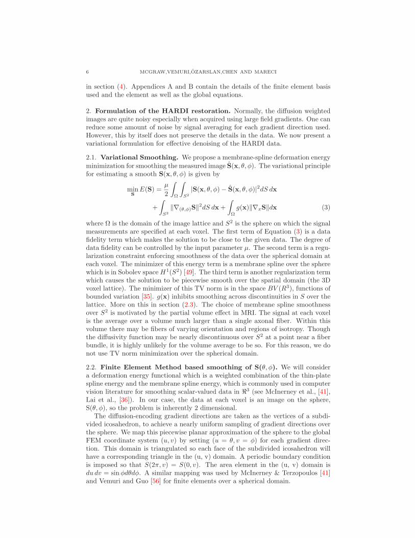
The element deformation energy due to virtual displacement z(u, v) is given by

Ejd = −

∫ ∫

Ωj

Njqjk(Njqj − z0) du dv. (16)

We can split the deformation energy into two terms : Ejd = qjT (Fjqj − f j) by

defining

Fj = −k

∫ ∫

Ωj

NjT Nj du dv (17)

and

f j = k

∫ ∫

Ωj

NjT z0 du dv. (18)

We may now balance the deformation energy and data energy by solving the fol-lowing linear system:

(Kj + Fj)qj = f j . (19)

The global linear system for smoothing the entire mesh may be obtained by ap-propriately summing the local element matrices, as detailed in Appendix B. Theglobal system is symmetric, and has a sparse banded structure with 18 nonzerodiagonal bands. Since the global matrix is positive-definite, an efficient solution toq is obtained via Cholesky factorization.

2.3. Spatial smoothing of S(x). We are now ready to describe the smoothing ofthe data across the 3D lattice. There are many existing methods that one can applyto this problem as discussed earlier. Smoothing the raw vector-valued data, S(x),is posed as a variational principle involving a first order smoothness constraint onthe solution to the smoothing problem. Note that the data at each voxel are mmeasurements of S over a sphere of directions and can be assembled into a vectorafter the smoothing on the spherical coordinate domain has been accomplished. Wepropose a weighted TV-norm minimization for smoothing this vector-valued imageS. This smoothing scheme reduces the effect of inter-region blurring, a drawbackGaussian convolution and isotropic diffusion suffer. Our method is a modified ver-sion of the work in Blomgren et. al., [11]. The novelty here lies in the choice of theweighting i.e., the coupling term between the channels. The variational principle forestimating a smooth S(x) is given by

minS

E(S) =

∫

Ω

(g(x)

m∑

i=1

‖∇Si‖ +µ

2

m∑

i=1

(Si − Si)2)dx (20)

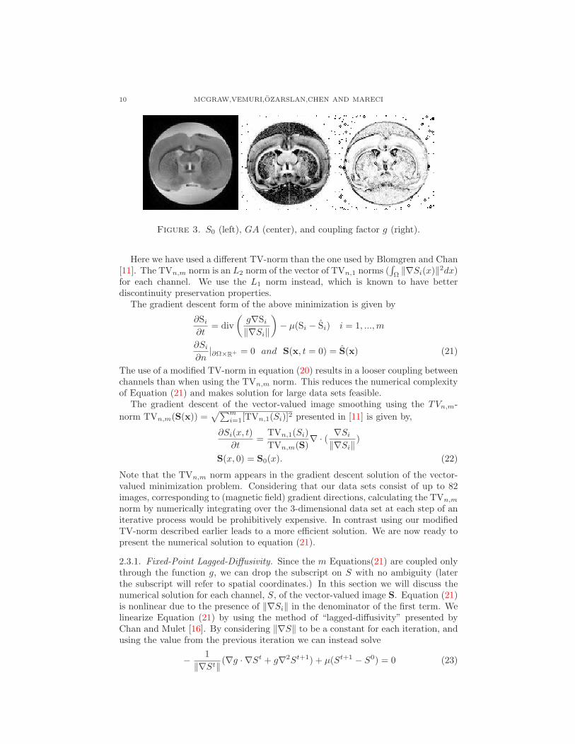
where, Ω is the image domain, µ is a regularization factor and m is the number ofimages. The first term here is the regularization constraint on the solution to have acertain degree of smoothness. The second term in the variational principle makes thesolution faithful to the data in the L2 sense. We have used the coupling functiong(x) = 1/(1 + ||∇GA(x)||2) for smoothing HARDI, where GA is the generalized

anisotropy index defined in Ozarslan et al., [45] and is computed from the varianceof normalized diffusivity. For a more detailed discussion on GA, we refer the readerto [45]. This selection criterion preserves edges in anisotropy while smoothing therest of the data. This anisotropy measure is chosen since it can be computed withoutexplicitly computing the ODF, and it is our goal to smooth the data prior to ODFcomputation. An image of the coupling term for a typical slice is shown in Figure(3).


Figure 3. S0 (left), GA (center), and coupling factor g (right).

Here we have used a different TV-norm than the one used by Blomgren and Chan[11]. The TVn,m norm is an L2 norm of the vector of TVn,1 norms (

∫

Ω‖∇Si(x)‖2dx)

for each channel. We use the L1 norm instead, which is known to have betterdiscontinuity preservation properties.

The gradient descent form of the above minimization is given by

∂Si

∂t= div

(

g∇Si

‖∇Si‖

)

− µ(Si − Si) i = 1, ...,m

∂Si

∂n|∂Ω×R

+ = 0 and S(x, t = 0) = S(x) (21)

The use of a modified TV-norm in equation (20) results in a looser coupling betweenchannels than when using the TVn,m norm. This reduces the numerical complexityof Equation (21) and makes solution for large data sets feasible.

The gradient descent of the vector-valued image smoothing using the TVn,m-

norm TVn,m(S(x)) =√

∑mi=1[TVn,1(Si)]2 presented in [11] is given by,

∂Si(x, t)

∂t=

TVn,1(Si)

TVn,m(S)∇ · ( ∇Si

‖∇Si‖)

S(x, 0) = S0(x). (22)

Note that the TVn,m norm appears in the gradient descent solution of the vector-valued minimization problem. Considering that our data sets consist of up to 82images, corresponding to (magnetic field) gradient directions, calculating the TVn,m

norm by numerically integrating over the 3-dimensional data set at each step of aniterative process would be prohibitively expensive. In contrast using our modifiedTV-norm described earlier leads to a more efficient solution. We are now ready topresent the numerical solution to equation (21).

2.3.1. Fixed-Point Lagged-Diffusivity. Since the m Equations(21) are coupled onlythrough the function g, we can drop the subscript on S with no ambiguity (laterthe subscript will refer to spatial coordinates.) In this section we will discuss thenumerical solution for each channel, S, of the vector-valued image S. Equation (21)is nonlinear due to the presence of ‖∇Si‖ in the denominator of the first term. Welinearize Equation (21) by using the method of “lagged-diffusivity” presented byChan and Mulet [16]. By considering ‖∇S‖ to be a constant for each iteration, andusing the value from the previous iteration we can instead solve

− 1

‖∇St‖ (∇g · ∇St + g∇2St+1) + µ(St+1 − S0) = 0 (23)


Here the superscript denotes iteration number. Equation (23) can be recast in theform

−∇2St+1 +µ‖∇St‖

gSt+1 =

µ‖∇St‖S0 + ∇g · ∇St

g. (24)

We now discretize the above equation in the following.

2.3.2. Discretized Equations. To write Equation (24) as a linear system (ASt+1 =f t), we discretize the Laplacian and gradient terms. Using central differences forthe Laplacian we have

∇2St+1 = St+1x−1,y,z + St+1

x,y−1,z + St+1x,y,z−1

− 6St+1x,y,z + St+1

x+1,y,z + St+1x,y+1,z + St+1

x,y,z+1 (25)

We define the standard central differences to be

∆xS =1

2(Sx+1,y,z − Sx−1,y,z)

∆yS =1

2(Sx,y+1,z − Sx,y−1,z)

∆zS =1

2(Sx,y,z+1 − Sx,y,z−1) (26)

We can rewrite Equation (24) in discrete form using the definitions in Equation (26)

−Sx−1,y,z − Sx,y−1,z − Sx,y,z−1

+(6 +µ√

(∆xSt)2+(∆ySt)2+(∆zSt)2

g)Sx,y,z

−Sx+1,y,z − Sx,y+1,z − Sx,y,z+1

= 1g(µS0

√

(∆xSt)2 + (∆ySt)2 + (∆zSt)2

+∆xg∆xSt + ∆yg∆ySt + ∆zg∆zSt) (27)

This results in a sparse linear system. The matrix of coefficients of St+1 has 7nonzero bands, and is given by

6 + µ‖∇St‖0

g0−1 . . . −1 . . . −1 . . .

−1 6 + µ‖∇St‖1

g1−1 . . . −1 . . . −1

0 −1 6 + µ‖∇St‖2

g2−1 . . . −1 . . .

. . .. . .

. . .. . .

. . . . . .. . .

. (28)

The matrix in Equation (28) is symmetric and diagonally dominant. We employthe conjugate gradient descent to solve this system. The solution of Equation (28)represents one fixed-point iteration. This iteration is continued until |St−St+1| < c,where c is a small prespecified tolerance.

2.4. Computing Probabilities. The probability in Equation (1) can now be eval-uated by computing the quantity S(q)/S0 and performing the FFT. If the sig-nal, S, is assumed to decay mono-exponentially from the origin of q-space (whereS(0) = S0), one can interpolate the signal values for arbitrary q. It is then pos-sible to extrapolate (using the monoexponential decay model) from the sphericalcoordinate locations to grid points in cartesian space and then perform the FFT onthis extrapolated data. The result is a probability of water molecule displacementover a small time constant. Since the quantity of interest is primarily the direc-tion of water displacement, one can integrate out the radial component of pt(r) to


get pt(θ, φ). This is commonly referred to as the diffusion orientation distributionfunction or simply ODF. Computing the ODF with this method is computationallyexpensive since it requires a 3D FFT at each voxel, and then a numerical integrationfor each direction. For the sake of efficiency, we will compute a probability profile(not the ODF), which will make processing large datasets feasible. This probabilityprofile, written as pt(r, θ, φ) quantifies the probability that a water molecule diffuses

through a sphere of fixed radius, r. A more detailed treatment by Ozarslan et al.can be found in [44]. This scheme provides a fast way to calculate the orientationprofiles. In our implementation we have evaluated the series given in [44] up tol = 6 terms since the reconstructed surfaces have very simple shapes which can beaccurately represented using a truncated spherical harmonics series, and r0 was setto 17.5µm. An alternative approach is to use the Funk-Radon Transform proposedby Tuch [51], however this introduces smoothing due to a spherical convolution stepwhich would make evaluation of our denoising algorithm more difficult.

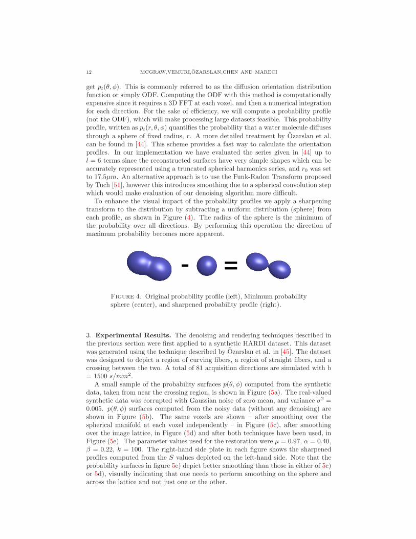
To enhance the visual impact of the probability profiles we apply a sharpeningtransform to the distribution by subtracting a uniform distribution (sphere) fromeach profile, as shown in Figure (4). The radius of the sphere is the minimum ofthe probability over all directions. By performing this operation the direction ofmaximum probability becomes more apparent.

Figure 4. Original probability profile (left), Minimum probabilitysphere (center), and sharpened probability profile (right).

3. Experimental Results. The denoising and rendering techniques described inthe previous section were first applied to a synthetic HARDI dataset. This datasetwas generated using the technique described by Ozarslan et al. in [45]. The datasetwas designed to depict a region of curving fibers, a region of straight fibers, and acrossing between the two. A total of 81 acquisition directions are simulated with b= 1500 s/mm2.

A small sample of the probability surfaces p(θ, φ) computed from the syntheticdata, taken from near the crossing region, is shown in Figure (5a). The real-valuedsynthetic data was corrupted with Gaussian noise of zero mean, and variance σ2 =0.005. p(θ, φ) surfaces computed from the noisy data (without any denoising) areshown in Figure (5b). The same voxels are shown – after smoothing over thespherical manifold at each voxel independently – in Figure (5c), after smoothingover the image lattice, in Figure (5d) and after both techniques have been used, inFigure (5e). The parameter values used for the restoration were µ = 0.97, α = 0.40,β = 0.22, k = 100. The right-hand side plate in each figure shows the sharpenedprofiles computed from the S values depicted on the left-hand side. Note that theprobability surfaces in figure 5e) depict better smoothing than those in either of 5c)or 5d), visually indicating that one needs to perform smoothing on the sphere andacross the lattice and not just one or the other.


Table 1. Error between ground-truth probabilities p and proba-bilities computed from restored synthetic data when SNR = 14.

Method µ(d(p, p)) σ(d(p, p))p = No Restoration 0.9409 0.2516

p = FEM Restoration 0.5540 0.1997p = TV Restoration 0.2840 0.2129

p = FEM + TV Restoration 0.1889 0.1748p = TV + FEM Restoration 0.2128 0.1631

Table 2. Error between ground-truth probabilities p and proba-bilities computed from restored synthetic data when SNR = 5.

Method µ(d(p, p)) σ(d(p, p))p = No Restoration 2.7461 0.3432

p = FEM Restoration 1.1848 0.2424p = TV Restoration 0.9175 0.1903

p = TV + FEM Restoration 0.4970 0.2046p = FEM + TV Restoration 0.6552 0.1984

From Figure (5b), it can be seen that the noise has a large influence on thesmoothness of the distribution. As expected from the variational formulation, thespikes of noise present in the raw data have been smoothed while preserving theoverall shape of the S profile. This smoothness is evident in the computed proba-bility profiles as well.

A quantitative evaluation can be obtained by comparing the distributions com-puted from the smoothed data with the ground-truth by using the square root ofJ-divergence (symmetrized KL-divergence) as a measure. This divergence is definedas

d(p, q) =√

J(p, q) (29)

where

J(p, q) =1

2

n∑

i=1

p(θi, φi) logp(θi, φi)

q(θi, φi)+ q(θi, φi) log

q(θi, φi)

p(θi, φi)(30)

In Table (1) we compare the distances, d(p, p), between the densities computedfrom the original synthetic data, (p), and the unrestored data, the data restoredonly using the FEM method, the data restored using only the TV-norm minimiza-tion, and the data restored using both techniques. For each technique, the meandistance, µ(d(p, p)), between the densities in corresponding voxels and the standarddeviation, σ(d(p, p)), is presented. As evident from Table (1), the TV restorationhas superior performance over the FEM technique in terms of the mean error. Thecombination of techniques has a lower mean error and standard deviation of theerror than either the L2-norm based or the TV-norm based restoration. Note alsothat the error achieved by applying smoothing over the sphere prior to smoothingover the voxel lattice is lower than when the order is reversed. Since TV-normminimization can be seen as a nonlinear diffusion process, performing the denois-ing in this order propagates smoothed intensities within homogeneous regions. Insubsequent experiments we perform the denoising in this order.


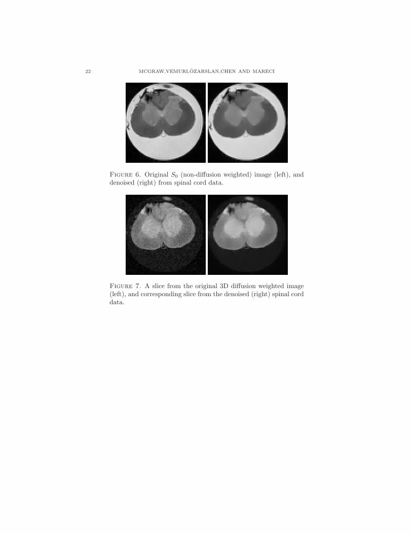
The denoising algorithm was applied to a dataset consisting of one non-diffusionweighted image and 46 diffusion weighted images of a rat spinal cord. Our data wereacquired using a 14.1 Tesla (600 MHz) Bruker Avance Imaging spectrometer systemwith a diffusion weighted spin echo pulse sequence. Imaging parameters were : TR= 1400 ms, TE = 25 ms, Delta = 17.5 ms, delta = 1.5 ms, bhigh = 1500s/mm2,blow = 0s/mm2, diffusion gradient strengths = 0 mT/m with 28 averages weremeasured for b = 0s/mm2 and diffusion gradient strengths = 733s/mm2 with 7averages were measured for each of the 46 diffusion weighting-gradient directions.The 46 directions were derived from the tessellation of a hemisphere. The image fieldof view was 4.3×4.3×12mm3, acquisition matrix was 72×72×40. The approximateSNR for the S0 and diffusion weighted images were 58 and 50 respectively. Theparameter values used for the restoration were µ = 0.97, α = 0.02, β = 0.0, k = 1.0.

Axial slices before and after denoising are shown for the non-diffusion weightedimage in Figure (6) and one diffusion weighted image in Figure (7). The ring-ing artifacts visible near the sample boundary in Figure (6) have been noticeablydecreased. Note that the edges in the image have been well preserved.

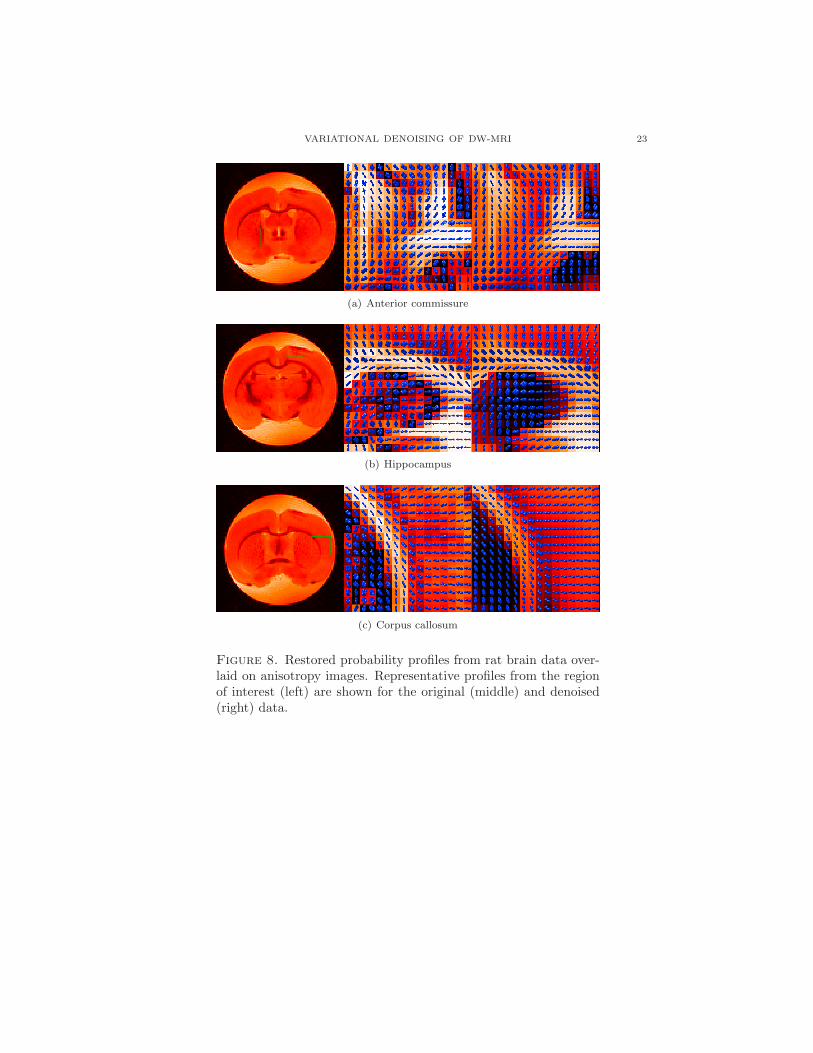
Figures (8) and (9) show restored probability profiles from rat brain and spinalcord datasets. The brain data were acquired using a 17.6 Tesla (750 MHz) BrukerAvance Imaging spectrometer system with a diffusion weighted spin echo pulsesequence. Imaging parameters were : TR = 2000 ms, TE = 28 ms, Delta = 17.8ms, delta = 2.2 ms, bhigh = 1500s/mm2, blow = 0s/mm2, 6 averages for each ofthe 81 diffusion weighting-gradient directions. The 81 directions were derived fromthe tessellation of a hemisphere. The image field of view was 150 × 150 × 300µm3,acquisition matrix was 100×100×60. The approximate SNR for the S0 and diffusionweighted images were 206 and 177 respectively.

Figure (8b) shows a detail from the rat hippocampus. The piecewise smoothingbehavior of the algorithm is evident within the anisotropic hippocampus region.This region has been smoothed independently of the more isotropic surroundingregions. The spherical smoothing term has also suppressed some peaks of the dis-tribution which were probably due to noise in the acquired data. Figure (8c) showsa detail from the rat corpus callosum. The data dependent coupling term in therestoration algorithm has permitted intraregion smoothing within the corpus callo-sum while preventing interregion smoothing. Note that the fiber directions withinthe corpus callosum have been well preserved.

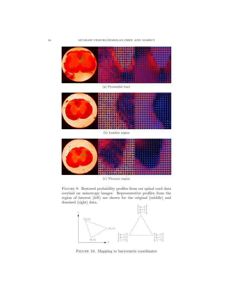
Figure (9) shows details from the rat spinal cord dataset. Here the noise reductioncan be seen to enhance the coherence of structures in the inner core of grey matter.

The data were processed by a MATLAB implementation of the algorithm run-ning on a system with Intel Quad Core QX6700 2.66 GHz CPU and 4 GB RAM.The computation times for the finite element smoothing over the sphere dependson the number of diffusion-encoding gradient directions in the image acquisition.For the spinal cord data with 46 directions the time was 0.018 seconds per voxel,and for the brain dataset with 81 directions the time was 0.038 seconds per voxel.The computation time for the TV-norm minimization problem for each diffusionweighted image depends on the size of the acquisition matrix. For the spinal cordthe resolution was 72 × 72 × 40 and the computation time per image was 28.3 sec-onds. For the brain dataset the resolution was 100 × 100 × 60 and computationrequired 82.4 seconds per image.


Table 3. Gauss-Radau weights

i ri wii ξi ai

1 0.0469100770 0.1184634425 0.0398098571 0.10079419262 0.2307653449 0.2393143353 0.1980134179 0.20845066723 0.5 0.2844444444 0.4379748102 0.26046339164 0.7692346551 0.2393143353 0.6954642734 0.24269359425 0.9530899230 0.1184634425 0.9014649142 0.1598203766

4. Conclusion. In this paper, we presented a new variational formulation forrestoring HARDI data and an FEM technique for implementing the restoration.Our formulation of the HARDI restoration involves two types of smoothness con-straints. The first is smoothness over the spherical domain of acquisition directions,and the second is smoothness between neighboring voxels in the Cartesian domain.The smoothing technique is capable of preserving discontinuities in the data. Thiswas demonstrated on synthetic and real anatomical data. By using J-divergence as ameasure of distance between distribution, we were able to show quantitatively thatthe combination of restoration techniques performs better than either techniquealone.

Appendix A.

Local Element Coordinates. We now present the coordinate system for thelocal elements. For local elements, triangular elements are used with a barycentriccoordinate system (γ, ξ, η). Each coordinate is in the range [0, 1] and γ + ξ + η = 1for points on the triangle.

The global coordinates, (u, v), can be computed from the local coordinates by[

uv

]

=

[

u1 − u0 u2 − u0

v1 − v0 v2 − v0

] [

ξη

]

+

[

u0

v0

]

. (31)

The Jacobian, J, of the transformation between coordinate systems is defined by

[

dudv

]

=

[

∂u∂ξ

∂u∂η

∂v∂ξ

∂v∂η

]

[

dξdη

]

= J

[

dξdη

]

. (32)

Integrals over the (u, v) domain to be converted to integrals over the local (ξ, η)domain by

∫ ∫

Ωj

f(u, v)du dv =

∫ ∫

Ωj

f(u(ξ, η), v(ξ, η)) det(J)dξ dη. (33)

Using the Gauss-Radau quadrature rules given in [26], we can approximate theintegral in Equation (33) by the summation

5∑

i=1

5∑

j=1

wiiwjjf(u(ξj , ηi,j), v(ξj , ηi,j)) det(J) (34)

where ηi,j = ri(1 − ξj), wjj = aj(1 − ξj), ξj , and wii are given in Table 3.


Derivatives over (u, v) can be written in terms of local coordinates by applyingthe chain rule:

∂N

∂u=

∂N

∂ξ

∂ξ

∂u+

∂N

∂η

∂η

∂u

∂N

∂v=

∂N

∂ξ

∂ξ

∂v+

∂N

∂η

∂η

∂v. (35)

The partial derivatives of ξ and η with respect to u and v can be computed byinverting the Jacobian

[

dξdη

]

=

[

∂ξ∂u

∂ξ∂v

∂η∂u

∂η∂v

] [

dudv

]

= J−1

[

dudv

]

. (36)

The inverse of J is given by

J−1 =1

det(J)

[

v2 − v0 −(u2 − u0)−(v1 − v0) u1 − u0

]

. (37)

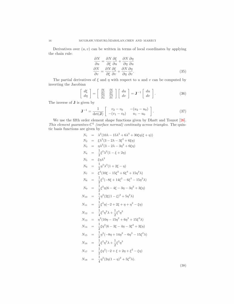
We use the fifth order element shape functions given by Dhatt and Touzot [26].This element guarantees C1 (surface normal) continuity across triangles. The quin-tic basis functions are given by

N1 = λ2(10λ − 15λ

2 + 6λ3 + 30ξη(ξ + η))

N2 = ξλ2(3 − 2λ − 3ξ

2 + 6ξη)

N3 = ηλ2(3 − 2λ − 3η

2 + 6ξη)

N4 =1

2ξ2λ

2(1 − ξ + 2η)

N5 = ξηλ2

N6 =1

2η2λ

2(1 + 2ξ − η)

N7 = ξ2(10ξ − 15ξ

2 + 6ξ3 + 15η

2λ)

N8 =1

2ξ2(−8ξ + 14ξ

2− 6ξ

3− 15η

2λ)

N9 =1

2ξ2η(6 − 4ξ − 3η − 3η

2 + 3ξη)

N10 =1

4η2(2ξ(1 − ξ)2 + 5η

2λ)

N11 =1

2ξ2η(−2 + 2ξ + η + η

2− ξη)

N12 =1

4ξ2η2λ +

1

2ξ3η2

N13 = η2(10η − 15η

2 + 6η3 + 15ξ

2λ)

N14 =1

2ξη

2(6 − 3ξ − 4η − 3ξ2 + 3ξη)

N15 =1

2η2(−8η + 14η

2− 6η

3− 15ξ

2λ)

N16 =1

4ξ2η2λ +

1

2ξ2η3

N17 =1

2ξη

2(−2 + ξ + 2η + ξ2− ξη)

N18 =1

4η2(2η(1 − η)2 + 5ξ

2λ).

(38)


The quintic shape functions have nodal variables which can be written in termsof local or global coordinates as,

qξ,η =

zzξ

zη

zξξ

zξη

zηη

,qu,v =

zzu

zv

zuu

zuv

zvv

. (39)

The local and global nodal variables are related to each other by

qu,v =

1 0 0 0 0 00 ξu ηu 0 0 00 ξv ηv 0 0 00 0 0 ξ2

u 2ξuηu η2u

0 0 0 ξuξv (ξuηv + ηuξv) ηuηv

0 0 0 ξ2v 2ξvηv η2

v

qξ,η. (40)

Appendix B.

Global Matrices. We wish to construct global matrices so that the energy balanceover the entire FEM mesh is given by the linear system

Kq = f (41)

where K is a (6n × 6n) matrix since we have 6 variables per node.We will consider the simple case of 2 elements. Expanding the element Equa-

tion(19) in terms of nodal variables for element 0 we get

K00,0 K0

0,1 K00,2

K01,0 K0

1,1 K01,2

K02,0 K0

2,1 K02,2

q00

q01

q02

=

f00

f01

f02

, (42)

and for element 1 we have

K13,3 K1

3,2 K13,1

K12,3 K1

2,2 K12,1

K11,3 K1

1,2 K11,1

q13

q12

q11

=

f13

f12

f11

. (43)

where each qjl is a (6 × 1) column vector of nodal variables. We expand each Kj

to be (6n× 6n) by inserting rows and columns of zeros corresponding to each nodeof the mesh. Also expand f j to (6n × 1). The global K and q are obtained bysumming the expanded matrices from each element in the mesh. For our 2 elementexample we have

K00,0 K0

0,1 K00,2 0

K01,0 K0

1,1 + K11,1 K0

1,2 + K11,2 K1

1,3

K02,0 K0

2,1 + K12,1 K0

2,2 + K12,2 K1

2,3

0 K13,1 K1

3,2 K13,3

q00

q01

q02

q03

=

f00

f01 + f1

1

f02 + f1

2

f03

. (44)

Acknowledgements. All MRI data was obtained at the Advanced Magnetic Res-onance Imaging and Spectroscopy (AMRIS) facility in the McKnight Brain Instituteat the University of Florida. This research was supported in part by the grant NIHEB7082 to BCV and by Siemens Corporate Research (Princeton, NJ). We wish tothank Sara Berens and Robert Yezierski for providing the spinal cord sample andRon Hayes for the brain.


REFERENCES

[1] H-E. Assemlal, D. Tschumperle, and L. Brun, Fiber tracking on HARDI data using robustODF fields, in ”IEEE International Conference on Image Processing” (2007), 344–351.

[2] H.-E. Assemlal, D. Tschumperle, and L. Brun, Robust variational estimation of pdf functionsfrom diffusion MR signal, in ”Computational Diffusion MRI Workshop held at the MedicalImage Computing and Computer-Assisted Intervention” (2008), 1–8.

[3] S.P. Awate and R.T. Whitaker, Feature-preserving MRI denoising: A nonparametric empir-ical bayes approach, IEEE Transactions on Medical Imaging 26 (2007), 1242–1255.

[4] P. J. Basser, New histological and physiological stains derived from diffusion-tensor MR im-ages, Ann. N Y Acad. Sci. 820 (1997), 123–138.

[5] P. J. Basser, Relationships between diffusion tensor and q-space MRI, Magn. Reson. Med. 47

(2002), 392–397.[6] P. J. Basser, J. Mattiello, and D. Le Bihan, MR diffusion tensor spectroscopy and imaging,

Biophys. J. 66 (1994), 259–267.[7] P. J. Basser, J. Mattiello, and D.Le Bihan, Estimate of the effective self-diffusion tensor from

the NMR spin echo, J. Magn. Reson. B (1994), 247–254.

[8] P. J. Basser, S. Pajevic, C. Pierpaoli, J. Duda, and A. Aldroubi, In vivo fiber tractographyusing DT-MRI data, Magn. Reson. Med. 44 (2000), 625–632.

[9] S. Basu, T. Fletcher, and R. Whitaker, Rician noise removal in diffusion tensor MRI., in“Medical Image Computing and Computer-Assisted Intervention”, (2006), 117–125.

[10] C. Beaulieu and P. S. Allen, Determinants of anisotropic water diffusion in nerves, Magn

Reson Med 31 (1994), 394–400.[11] P. Blomgren and T. F. Chan, Color TV: total variation methods for restoration of vector-

valued images, IEEE Transactions on Image Processing 7 (1998), 304–309.

[12] I. Bogdanova, X. Bresson, J.P. Thiran, and P. Vandergheynst, Scale space analysis and activecontours for omnidirectional images, IEEE Transactions On Image Processing 16 (2007),

1888–1901.[13] P.T. Callaghan, “Principles of Nuclear Magnetic Resonance Microscopy”, Clarendon Press,

Oxford, 1991.

[14] C.A. Castano-Moraga, C. Lenglet, R. Deriche, and J. Ruiz-Alzola, A Riemannian approachto anisotropic filtering of tensor fields, Signal Processing 87 (2007), 263–276.

[15] T. Cecil, S. Osher, and L. Vese, Numerical methods for minimization problems constrainedto S1 and S2, Journal of Computational Physics 198 (2004), 567–579.

[16] T. Chan and P. Mulet, On the convergence of the lagged diffusivity fixed point method in total

variation image restoration, SIAM Journal on Numerical Analysis 36 (1999), 354–367.[17] C. Chefd’hotel, D. Tschumperle, R. Deriche, and O. Faugeras, Regularizing flows for con-

strained matrix-valued images, Journal of Mathematical Imaging and Vision 20 (2004), 147–162.

[18] C. Chefd’hotel, D. Tschumperle, R. Deriche, and O. D. Faugeras, Constrained flows of matrix-

valued functions: Application to diffusion tensor regularization, European Conference onComputer Vision 1 (2002), 251–265.

[19] B. Chen and E.W. Hsu, Noise Removal in Magnetic Resonance Diffusion Tensor Imaging,Magnetic Resonance In Medicine 54 (2005), 393–401.

[20] Y. Chen, W. Guo, Q. Zeng, X. Yan, F. Huang, H. Zhang, G. He, B. C. Vemuri, and Y. Liu,

Estimation, smoothing, and characterization of apparent diffusion coefficient profiles fromhigh angular resolution DWI., in “Computer Vision and Pattern Recognition”, (2004), 588–

593.[21] R. A. Clarke, P. Scifo, G. Rizzo, F. DellAcqua, G. Scotti, and F. Fazio, Noise correction on

Rician distributed data fibre orientation estimators, IEEE Transactions Medical Imaging 27

(2008), 1242–1251.[22] T. E. Conturo, N. F. Lori, T. S. Cull, E. Akbudak, A. Z. Snyder, J. S. Shimony, R. C.

McKinstry, H. Burton, and M. E. Raichle, Tracking neuronal fiber pathways in the living

human brain, Proc. Natl. Acad. Sci. 96 (1999), 10422–10427.[23] M. Descoteaux, E. Angelino, S. Fitzgibbons, and R. Deriche, A fast and robust odf estimation

algorithm in q-ball imaging, in “International Symposium on Biomedical Imaging: From Nanoto Macro”, (2006), 81–84.

[24] M. Descoteaux, E. Angelino, S. Fitzgibbons, and R. Deriche, Regularized, fast, and robust

analytical Q-ball imaging, Magnetic Resonance In Medicine 58 (2007), 497–510.

http://www.ams.org/mathscinet-getitem?mr=MR2463092&return=pdf





[25] M. Descoteaux, N. Wiest-Daessle, S. Prima, C. Barillot, and R. Deriche, Impact of rician

adapted non-local means filtering on HARDI, in “Medical Image Computing and Computer-Assisted Intervention”, (2008), 122–130.

[26] G. Dhatt and G. Touzot, “The Finite Element Method Displayed”, Wiley, New York, 1984.

[27] C. Feddern, J. Weickert, B. Burgeth, and M. Welk, Curvature-Driven PDE Methods forMatrix-Valued Images, International Journal of Computer Vision 69 (2006), 93–107.

[28] P. Fillard, V. Arsigny, X. Pennec, and N. Ayache, Clinical DT-MRI estimation, smoothingand fiber tracking with log-Euclidean metrics, IEEE Transactions on Medical Imaging 26

(2007), 1472–1482.

[29] L. R. Frank, Anisotropy in high angular resolution diffusion-weighted MRI, Magn Reson Med45 (2001), 935–939.

[30] L. R. Frank, Characterization of anisotropy in high angular resolution diffusion-weightedMRI, Magn Reson Med 47 (2002), 1083–1099.

[31] Y. Gur and N. Sochen, Denoising tensors via lie group flows, Variational, Geometric, and

Level Set Methods in Computer Vision 3752 (2005), 13–24.[32] G. Hamarneh and J. Hradsky, Bilateral Filtering of Diffusion Tensor Magnetic Resonance

Images, IEEE Transactions On Image Processing 16 (2007), 2463–2475.

[33] K. M. Jansons and D. C. Alexander, Persistent angular structure: new insights from diffusionmagnetic resonance imaging data, Inverse problems 19 (2003), 1031–1046.

[34] D. K. Jones, A. Simmons, S. C. R. Williams, and M. A. Horsfield, Non-invasive assessmentof axonal fiber connectivity in the human brain via diffusion tensor MRI, Magn. Reson. Med.42 (1999), 37–41.

[35] E. Fatemi L. Rudin, S. Osher, Nonlinear total variation based noise reduction algorithms,Physica D 60 (1992), 259–268.

[36] S.-H. Lai and B. C. Vemuri, Physically based adaptive preconditioning for early vision., IEEETrans. Pattern Anal. Mach. Intell. 19 (1997), 594–607.

[37] L. Lui, Y. Wang, and TF Chan, Solving PDEs on manifold using global conformal param-

eterization, in “Variational, Geometric, and Level Set Methods in Computer Vision: ThirdInternational Workshop”, (2005), 307–319.

[38] N. Makris, A. J. Worth, A. G. Sorensen, G. M. Papadimitriou, O. Wu, T. G. Reese, V. J.Wedeen, and et al, Morphometry of in vivo human white matter association pathways withdiffusion-weighted magnetic resonance imaging, Ann. Neurol. 42 (1999), 951–962.

[39] T. McGraw, B. C. Vemuri, Y. Chen, M. Rao, and T. Mareci, DT-MRI denoising and neuronalfiber tracking, Medical Image Analysis 8 (2004), 95–111.

[40] T. McGraw, B.C. Vemuri, Z. Wang, Y. Chen, M. Rao, and T. Mareci, Line integral con-volution for visualization of fiber tract maps from DTI, in “Medical Image Computing andComputer-Assisted Intervention”, (2002), 615–622.

[41] T. McInerney and D. Terzopoulos, A dynamic finite element surface model for segmenta-tion and tracking in multidimensional medical images with application to cardiac 4D image

analysis, Comp. Med. Imag. Graph. 19 (1995), 69–83.[42] S. Mori, B. J. Crain, V. P. Chacko, and P. C. M. van Zijl, Three-dimensional tracking of axonal

projections in the brain by magnetic resonance imaging, Ann. Neurol. 45 (1999), 265–269.

[43] E. Ozarslan and T. H. Mareci, Generalized diffusion tensor imaging and analytical relation-

ships between diffusion tensor imaging and high angular resolution diffusion imaging, MagnReson Med 50 (2003), 955–965.

[44] E. Ozarslan, T. M. Shepherd, B. C. Vemuri, S. J. Blackband, and T. H. Mareci, Resolu-tion of complex tissue microarchitecture using the diffusion orientation transform (DOT),

NeuroImage 31 (2006), 1086–1103.

[45] E. Ozarslan, B. C. Vemuri, and T. H. Mareci, Generalized scalar measures for diffusion MRIusing trace, variance and entropy, Magn Reson Med 53 (2005), 866–876.

[46] P. Savadjiev, J. S. W. Campbell, G. B. Pike, and K. Siddiqi, 3d curve inference for diffusionMRI regularization and fibre tractography, Medical Image Analysis 10 (2006), 799–813.

[47] E. O. Stejskal and J. E. Tanner, Spin diffusion measurements: Spin echoes in the presence

of a time-dependent field gradient, J. Chem. Phys. 42 (1965), 288–292.[48] B. Tang, G. Sapiro, and V. Caselles, Diffusion of general data on non-flat manifolds via har-

monic maps theory: The direction diffusion case, International Journal of Computer Vision

36 (2000), 149–161.[49] D. Terzopoulos, Regularization of inverse visual problems involving discontinuities, IEEE

Transactions on Pattern Analysis and Machine Intelligence 8 (1986), 413–242.




[50] D. Tschumperle and R. Deriche, Variational frameworks for DT-MRI estimation, regulariza-

tion and visualization, International Conference on Computer Vision (2003), 116–121.[51] D. S. Tuch, Q-ball imaging, Magn Reson Med. 52 (2004), 1358–1372.[52] D. S. Tuch, T. G. Reese, M. R. Wiegell, and V. J. Wedeen, Diffusion MRI of complex neural

architecture, Neuron 40 (2003), 885–895.[53] D. S. Tuch, R. M. Weisskoff, J. W. Belliveau, and V. J. Wedeen, High angular resolution diffu-

sion imaging of the human brain, Proc. of the 7th Annual Meeting of ISMRM (Philadelphia,PA), 1999, p. 321.

[54] B. C. Vemuri, Y. Chen, M. Rao, T. McGraw, Z. Wang, and T. Mareci, Fiber tract mapping

from diffusion tensor MRI, in “Proceedings of the IEEE Workshop on Variational and LevelSet Methods”, (2001), 81–88.

[55] B. C. Vemuri, Y. Chen, M. Rao, Z. Wang, T. McGraw, T. Mareci, S. J. Blackband, andP. Reier, Automatic fiber tractography from DTI and its validation, in “IEEE Intl. Symp. onBiomedical Imaging”, (2002), 501–504.

[56] B. C. Vemuri and Y. Guo, Snake pedals: Compact and versatile geometric models withphysics-based control, IEEE Trans. Pattern Anal. Mach. Intell. 22 (2000), 445–459.

[57] Z. Wang, B. C. Vemuri, Y. Chen, and T. H. Mareci, A constrained variational principle for

direct estimation and smoothing of the diffusion tensor field from DWI., in “InformationProcessing in Medical Imaging”, (2003), 660–671.

[58] Z. Wang, B. C. Vemuri, Y. Chen, and T. H. Mareci, A constrained variational principlefor direct estimation and smoothing of the diffusion tensor field from complex DWI, IEEETransactions on Medical Imaging 23 (2004), 930–939.

[59] V. J. Wedeen, T. G. Reese, D. S. Tuch, M. R. Weigel, J. G. Dou, R.M. Weiskoff, andD. Chessler, Mapping fiber orientation spectra in cerebral white matter with Fourier transform

diffusion MRI, in “Proc. of the 8th Annual Meeting of ISMRM”, 2000, 82.[60] J. Weickert and T. Brox, Diffusion and regularization of vector- and matrix-valued images,

Contemporary Mathematics 313 (2002), 251–268.

[61] N. Wiest-Daessle, S. Prima, P. Coupe, S. P. Morrissey, and C. Barillot, Rician noise removalby non-local means filtering for low signal-to-noise ratio MRI: Applications to DT-MRI, in

“Medical Image Computing and Computer-Assisted Intervention”, (2008), 171–179.[62] N. Wiest-Daessle, S. Prima, P. Coupe, S.P. Morrissey, and C. Barillot, Non-local means vari-

ants for denoising of diffusion-weighted and diffusion tensor MRI, Medical Image Computing

and Computer-Assisted Intervention 4792 (2007), 344.[63] R. Xue, P. C. M. van Zijl, B. J. Crain, H. Solaiyappan, and S. Mori, In vivo three-dimensional

reconstruction of rat brain axonal projections by diffusion tensor imaging, Magn. Reson. Med.42 (1999), 1123–1127.

Received xxxx 20xx; revised xxxx 20xx.

E-mail address: [email protected]






(a) Original synthetic data

(b) Added Gaussian noise, σ2 = 0.005,

SNR = 14

(c) Manifold smoothing with α = 0.01

(d) Lattice smoothing with µ = 0.95 (e) Manifold smoothing followed byLattice smoothing

(f) Added Gaussian noise, σ2 = 0.04,

SNR = 5(g) Manifold smoothing with α = 0.01

(h) Lattice smoothing with µ = 0.95 (i) Manifold smoothing followed by

Lattice smoothing

Figure 5. Simulations from a 64×64 synthetic high angular reso-lution diffusion image, subsampled for display purposes. The signalprofiles, S(θ, φ), are shown on the left side of each panel whereasthe probability profiles are provided on the right. Results frommanifold smoothing using FEM, lattice smoothing using TV-normminimization, and a combination of the two techniques are shownfor noisy data.


Figure 6. Original S0 (non-diffusion weighted) image (left), anddenoised (right) from spinal cord data.

Figure 7. A slice from the original 3D diffusion weighted image(left), and corresponding slice from the denoised (right) spinal corddata.


(a) Anterior commissure

(b) Hippocampus

(c) Corpus callosum

Figure 8. Restored probability profiles from rat brain data over-laid on anisotropy images. Representative profiles from the regionof interest (left) are shown for the original (middle) and denoised(right) data.


(a) Pyramidal tract

(b) Lumbar region

(c) Thoracic region

Figure 9. Restored probability profiles from rat spinal cord dataoverlaid on anisotropy images. Representative profiles from theregion of interest (left) are shown for the original (middle) anddenoised (right) data.

u

v

(u0, v0)

(u1, v1)

(u2, v2)

ξ0 = 0η0 = 0γ0 = 1

ξ1 = 1η1 = 0γ1 = 0

ξ2 = 0η2 = 1γ2 = 0

Figure 10. Mapping to barycentric coordinates

Documents

Tim McGraw Baba Vemuri Evren Ozarslan¨ Yunmei Chen …web.ics.purdue.edu/~tmcgraw/papers/mcgraw_variational_2009.pdf · 2 MCGRAW,VEMURI,OZARSLAN,CHEN AND MARECI¨ gradient directions