Embed Size (px)
Citation preview

Time as a Trade Barrier
By DAVID L. HUMMELS AND GEORG SCHAUR*
A large and growing share of international trade is carried on
airplanes. We model firms’ choice between exporting goods using
fast but expensive air cargo and slow but cheap ocean cargo. This
choice depends on the price elasticity of demand and the value that
consumers attach to fast delivery and is revealed in the relative
market shares of firms who air and ocean ship. We use US imports
data that provide rich variation in the premium paid for air
shipping and in time lags for ocean transit to identify these
parameters and extract consumer’s valuation of time. By exploiting
variation across US entry coasts we are able to control for selection
and for unobserved shocks to product quality and variety that affect
market shares. We estimate that each day in transit is equivalent to
an ad-valorem tariff of 0.6 to 2.1 percent and that the most time-
sensitive trade flows are those involving parts and components
trade. Our estimates are useful for understanding the impact of
sharp declines in air cargo prices on the composition and
organization of trade, and also useful for assessing the economic
impact of policies that raise or lower time to trade such as security
screening of cargo, port infrastructure investment, or streamlined
customs procedures.
* Hummels: Purdue University and NBER, 100 S. Grant Street, West Lafayette, IN 47907 (email:
[email protected]). Schaur: The University of Tennessee, 916 Volunteer Blvd., Knoxville, TN 37996 (email:

[email protected]). For many helpful comments and discussions we thank seminar audiences at NBER, EIIT, Midwest
Meetings, The World Bank, the Universities of Michigan, Maryland, Colorado, Purdue, Virginia Tech, Indiana University,
Rotterdam and the Minneapolis Fed, and are especially indebted to Jason Abrevaya, Andrew Bernard, Bruce Blonigen,
Alan Deardorff, Pinelopi Goldberg, James Harrigan, Tom Hertel, Pete Klenow, Christian Vossler, Kei-Mu Yi, and two
anonymous referees. We are grateful for funding under NSF Grant 0318242, and from the Global Supply Chain
Management Initiative. All errors remain our own. The authors have received consulting fees from US Agency for
International Development, through the consulting firm Nathan and Associates, for providing calculations related to this
paper. Specifically, the estimates of “time costs” developed in an early draft of this paper were used to calculate the tariff
equivalent of port delays in various countries. None of the funding sources or interested parties reviewed this paper prior to
its circulation.
Moving traded goods over long distances takes time. Ocean-borne cargo
leaving European ports takes an average of 20 days to reach US ports and 30 days
to reach Japan. Air borne cargo requires only a day or less to most destinations,
but it is also much more expensive. In 2005, goods imported into the US faced per
kilogram charges for air freight that were, on average, 6.5 times higher than ocean
freight charges.
Despite the expense, a large and growing fraction of world trade travels by air.
From 1965-2004, worldwide use of air cargo grew 2.6 times faster than use of
ocean cargo.1 In 2000, airborne trade for the US amounted to 36 percent of
import value and 58 percent of export value for countries outside North America.2
In sum, airplanes are fast, expensive, and increasingly important to trade. In this
paper we examine two hypotheses suggested by these facts: lengthy shipping
times impose costs that impede trade and firms engaged in trade exhibit
significant willingness-to-pay to avoid these costs.
What are these time costs? Lengthy shipping times impose inventory-holding
and depreciation costs, which could include literal spoilage (fresh produce or cut
1 Hummels (2007) calculates that worldwide use of airborne cargo (measured in kg-km) grew 11.7 percent per year
from 1965-2004 compared to 4.4 percent per year for ocean cargo. The much shorter sample of US imports that we employ in the empirical section shows a growing share of air shipments from 1991 to 2000, after which the air share falls through
2005 (see Figure 1). 2
Cristea et al (2011) provide systematic data on trade by transport mode for many countries in 2004. For example, in
2004, air cargo as a share of export value was 29 percent for the UK, 42 percent for Ireland, and 51 percent for Singapore; 22 percent of Argentine and 32 percent of Brazilian imports were airborne
flowers), or rapid technological obsolescence for goods such as consumer
electronics. Timeliness is potentially important in the presence of demand
uncertainty.3 Long lags between ordering and delivery require firms to commit to
product specifications and quantities supplied before uncertain demand is
resolved. Rapid transport on airplanes can allow firms to shorten response times
and use late arriving information.
Time costs may be magnified in the presence of multi-stage global supply
chains. Inventory-holding and depreciation costs for early-stage value-added
accrue throughout the duration of the production chain, and demand uncertainty
can ripple throughout upstream stages. Perhaps most importantly, the absence of
key components due to late arrival or quality defects can idle an entire assembly
plant, making the ability to ship rapidly worth potentially many times the value of
the components being transported.4
In this paper we examine the modal choice decisions of firms engaged in trade
and use the trade-off between fast and expensive air transport versus slow and
inexpensive ocean shipping to identify the value of time saving. In the model
consumers have preferences over goods that are differentiated along both
horizontal and quality dimensions, and slow delivery reduces consumers’
perception of product quality. Producers can improve perceived quality by paying
a premium to air ship. Unit shipping costs imply that the air freight premium,
measured in ad-valorem terms, is decreasing in product prices. That is, high price
firms incur a smaller increase in delivered prices when they upgrade perceived
quality using airplanes, and are more likely to air ship goods, while low price
firms are more likely to employ ocean shipping.
3 See Aizenman (2004), Evans and Harrigan (2005), and Hummels and Schaur (2010) and the appendix for details.
4 Harrigan and Venables (2006) argue that this is an important force driving economic agglomeration, but firms need
not cluster geographically if long distances can be rapidly bridged with airplanes.

Consumers’ valuation of time is then revealed in the relative revenues of the
two types of firms. Purchases of air shipped varieties are decreasing in proportion
to the premium paid to air ship, and, conditional on prices, increasing in
proportion to consumers’ valuation of time. This revenue shifting will be
strongest when demand is more price elastic and when the time delays are
greatest. A consumer buying goods from a nearby exporter may be unwilling to
pay the air premium to save a few days in transit, but that same consumer will pay
the air premium if the exporter is many weeks of ocean travel away. By
combining our estimates of these two effects we can extract the price-equivalent
of the consumers’ valuation of each day of delay.
To estimate this model we use data on US imports from 1991-2005 that allow
us to construct, for air and ocean modes, measures of revenues, prices, shipping
costs, and numbers of shipments that are specific to each exporting country x HS
6 digit product x US entry coast x year. We combine this with a detailed ocean
shipping schedule for all ocean vessels worldwide that provides us with shipping
times for each exporter x US entry coast. We then relate relative (air/ocean)
revenues to relative prices, relative shipping costs and time delays. We exploit
variation in the price/speed trade off across countries, products, entry coast and
time in order to identify consumers’ willingness to pay for time savings.
The rich structure of the data allows us to address problems related to selection,
the extensive margin expansion of trade, and unobserved characteristics of
exporters and products including quality differentiation and inland or port
infrastructure. High trade costs induce firms to select out of markets so that
regressions of export sales on trade costs incorporate both this selection effect and
an extensive margin (number of firms trading) response to the costs. We control
for selection with a two-step estimator that uses the exporter’s sales to the world
(less the US) for each product x year to predict the probability that it will sell that
product to the US. We control for the extensive margin using data on the number

of shipments so that the normalized dependent variables are akin to average sales
per firm.
A recent literature emphasizes the importance of quality differentiation in trade,
where quality is typically measured either as price variation or as a residual of
quantity demanded controlling for prices. Unlike this literature we have an
explicit measure of one aspect of quality, timely delivery, for which we directly
estimate consumers’ valuation. In addition, we employ various fixed effect
estimators to provide strong controls for unobserved quality and variety (the
number of firms shipping a good) that affect relative revenues.
In the most robust treatment we exploit variation across US entry coasts.
European ocean cargoes arriving on the US west coast must traverse the Panama
Canal and take 10-14 days longer to arrive than those reaching the east coast (and
vice versa for Asia). We can then hold fixed hold fixed unobservables that are
specific to an exporter x product x time and exploit this quirk of geography to
generate variation across US coasts in the relative share of air shipping as a
function of relative time delays, and relative freight prices. This allows us to
control for unobserved quality variation in a manner that is considerably more
general than what is found in the literature on estimating import demand
elasticities or in the literature on quality and trade. It also permits us to hold fixed
the characteristics of exporters – their geography, income, infrastructure – that
may affect usage of air shipments.
We find that air/ocean revenues are high when the air freight premium is low,
and when shipment lags are long. In the pooled specifications we estimate that
each day in transit is worth from 0.6 to 2.1 percent of the value of the good. We
also estimate the model separately for each End-Use category and find
considerable heterogeneity across products in time sensitivity. The most striking
result from the disaggregated product regressions is that parts and components
have a time sensitivity that is 60 percent higher than other goods.
While our estimates are based on transport modal choice, they are informative
about many policies and sources of technological change that speed goods to
market. For example, imposing strict port security procedures could significantly
slow the flow of goods into the domestic market, while investing in more efficient
port infrastructure may allow goods to reach their destinations more quickly and
boost trade.5
Our estimates also have implications for changing patterns of trade and the
international organization of production. In the post-war era, world trade has
grown much faster than output with typical explanations attributing this growth to
declining tariffs and improved technology (information and transportation). To
the extent that time is a barrier to trade, declines in air shipping prices may help
explain both aggregate trade growth and a shift toward trade in especially time
sensitive goods or forms of production organization. As an example, an important
recent feature of trade is especially rapid growth in the fragmentation of
production. Our estimates show that parts and components are among the most
time sensitive products. This suggests that the rapid declines in air transport
costs, and the corresponding reduction in the cost of time-saving, may be
responsible for the growth of time and coordination-intensive forms of
integration.
The paper proceeds as follows. Section I models the firm’s choice of shipping
mode and generates predictions for relative export revenues. Section II describes
the data and specification issues in estimation. Section III provides results.
Section IV concludes. An appendix available online provides further detailed
description of the related literature, model derivations, sample construction, and
robustness checks.
5 Employing aggregate data and a different methodology Djankov et al (2010) identify the cost of a day’s delay in
inland transit in terms of trade value. Their cost estimates are similar to ours in magnitude. This suggests that the cost of
delay is similar whether it occurs on land or sea, even though there is no technical reason for why the two different approaches should deliver the same estimate.

I. Theory
In our data we see exporter-by-product trade flows into the U.S. disaggregated
by transportation mode -- air and ocean vessel. In many instances, data for a
single trade flow indicates that both air and ocean modes were used in the same
time period. For other flows, only air or ocean are employed in a single time
period, with modal choice varying across exporters, products, and years. We
provide a simple theoretical structure that yields these outcomes in order to
organize our analysis of modal use and its implications for the value of time
savings.
We focus on US import demands within a narrow product category. All
variables below are product specific, so we suppress product and destination
superscript for notational ease, reintroducing it where appropriate in the empirical
section. Import demand is CES across varieties, summed across export locations j
and across firms z within each location j,
1/
z z
j jj iU q
1 /
where is the elasticity of substitution between goods and
exp( )z z z
j j jdays is a price-equivalent demand shifter that depends on a
firm z, location j-specific quality, z
j , and a term exp( )z
jdays that captures the
consumer disutility of slow delivery.
This formulation of demand is similar to the literature on quality in trade,
including Hallak (2006), Hummels-Klenow (2005), and Hallak-Schott (2011),
with the exception that these papers treat all elements of quality as unobservable.
In contrast, we measure timeliness as an important measurable component of

quality. Time in transit, ( ) jdays z , depends on exporter location because of
differences in distance to the import market and infrastructure quality, but also on
the endogenous choice of firm z to pay a premium for timely delivery.
With real expenditures on product k given by E, demands for firm z from
exporter j, selling at a delivered price *z
jp are
(1) *
= .exp( )
z
jz
j z z
j j
pq E
days
Other things equal, a consumer gets more utility from a good that arrives sooner
rather than later, which is expressed by increasing demand for that good. A 1%
price reduction raises demand by %, and a 1 day reduction in delivery times
raises demand by . That is, the time valuation parameter translates days of
delay into a price (or tariff) equivalent form, and the elasticity of substitution
translates this into the quantity of lost sales.
Turning to the production side of the model, the firm z marginal cost of
delivering a product from export location j to the market via mode m=air,ocean is
m
jz g , where z is the marginal cost of production (potentially correlated with
unobserved quality z
j ) and m
jg is a shipping charge proportional to the quantity,
not the value shipped (see Hummels-Skiba 2004 for evidence on this point). Air
shipping is more expensive than ocean shipping, A O
j jg g .
The firm pays fixed costs FC at the beginning of the period and commits to a
mode of transportation. The firm charges prices that are a markup over marginal
costs, * ( ) /z m
j jp z g . Multiplying by the quantity demanded from (1) and
subtracting fixed and variable costs yields

(2) ( ) ( ) /
( ) =1 exp( )
m m
j jm
j z m
j j
z g z gz E FC
days
To determine the optimal transport mode the firm compares the profitability of
air versus ocean shipping. The firm chooses air if ( ) > ( )a o
j jz z . Taking logs of
(2), assuming that airborne cargoes can reach their destination in one day, and
simplifying implies
(3) (1 ) ln( ) ln( ) 1 > 0a o o
j j jz g z g days
Equation (3) shows that a firm trades the greater expense of air shipping against
the improved “quality” of a product that arrives 1o
jdays earlier. Long ocean
shipping times are more likely to induce a switch to air shipping when consumers
attach greater value to timeliness, and when goods are closer substitutes. The
latter effect operates because we have defined in price equivalent terms in
order to measure the effect of timeliness on quantities shipped. Higher elasticities
of substitution translate into larger quantity effects.
The additive form of shipping costs also implies that modal choice depends on
marginal costs of production. Since >a o
j jg g , using air shipping always results in
a higher delivered price, but the magnitude of this difference -- the impact that the
air shipping premium has on delivered prices -- is decreasing in marginal costs of
production. To see the intuition, suppose a pair of shoes can be shipped by air for
$11 or by ocean for $1. The air freight premium doubles the price of $9 shoes but
increases the price of $99 shoes by only 10 percent. Ceteris paribus, higher value
goods will be more likely to use air shipping.

Exporting occurs if for the optimal mode, profits from exporting exceed fixed
costs, or
(4) (1 ) ln( ) ln ( ) lnm m
j j jz g days FC
This defines a selection equation indicating whether or not a particular location
successfully exports a product to the importer and appears in the data.
From this, we can derive two cases that correspond to modal-use patterns in the
data. For a single firm it will be optimal to choose either air or ocean shipping.
As we show in the online appendix, it is straightforward to derive a probit model
from equation (3) relating the probability of air shipment to relative shipping
prices and days in transit. If all variables are observed we can extract consumers’
valuation of time saving from that model. However, this case poses two
significant challenges for estimation: we do not observe shipping costs for the
transport mode not chosen and we cannot control for unmeasured product quality
variation.
Consider a second case. National trade data aggregates over multiple firms.
Suppose we have two firms from exporter j with different marginal costs such that
one firm (denoted “o”) ocean ships and the other (denoted “a”) air ships. Firm o
generates export revenues inclusive of shipping charges
(5)
11
* = ( )exp( ) 1
o o o
j jo o
j j
r E z gdays
and similarly for firm a. Writing the revenue equation (5) in relative terms we
can transform the expressions so that all variables are observable in the data
(details available in the online appendix). Denoting origin prices as m
jp , and ad-

valorem shipping costs as = 1 /m m m
j j jf g p we have an expression for revenues
(exclusive of shipping costs).
(6) ( )
ln ( 1) (1 ) ln ln ln( )
a a a a
j j j jo
jo o o o
j j j j
r z p f vdays
r z p f v
Equation (6) captures a trade-off similar to that in equation (3), only expressed
in revenue rather than probability terms. Consumers view goods from the two
firms as imperfect substitutes, and alter their relative purchases as a function of
relative price and relative quality. We identify this in the data as a tradeoff –
ocean shipped goods have lower costs but are perceived by consumers to be of
lower quality because they arrive days or weeks later than an air shipped good.
The cost difference induces larger movements in revenues when is large (the
goods are close substitutes). Time delays induce larger movements in revenues
when is large and consumers have a higher valuation for timeliness, .
Combining estimates of and we can extract consumers’ willingness to pay
for timely delivery. Finally, we account for the possibility that consumers may
also perceive a quality difference between the two types of firms that is unrelated
to timeliness. This appears as the last term in equation (6). We discuss this, and
the endogeneity of ad-valorem shipping charges, at length in Section II.
Equation (6) generalizes to the case of many firms. Let m
jN denote the number
of firms of type m
jz , and write aggregate revenues ( )m
jR z as an aggregation over
all firms that export using mode m6. In relative terms, aggregate revenues are
6 We show in the online appendix that equation (7) is a second order approximation of a model in which heterogenous
firms draw marginal costs z from a distribution as in Melitz (2003). In that case the mass (number) of firms in each mode
adjusts continuously in response to changes in time delays and shipping costs, and the included variables for cost and quality are weighted averages over the firms in each mode

(7) ( ) ( )
= ( 1) (1 ) ln ln ln( ) ( )j
a a a a a a a
j j j j j j jo
jo o o o o o o
j j j j j j
R z N r z p f v Ndays
R z N r z p f v N
The distinction between revenues per firm and revenues aggregated over m
jN
firms displays the potential importance of a modal extensive margin – defined not
as the number of firms exporting but the number of firms within an industry that
export using a given mode of transportation.
II. Data and Specifications
A. Data
We employ data from the U.S. Imports of Merchandise database, 1991-2005,
with sample construction details reported in the appendix. When taking equations
(6) and (7) to the data, an observation is an HS6 digit good k (roughly 5000
distinct products), exported from country j, arriving at US coast c (c=west, east),
via mode m (m=air,ocean) in year t. We have quantities (in kg), the total value of
the shipments (in US$), shipping charges (US$), and number of distinct shipment
records for each j-k-c-t trade flow.
Table 1 reports data on the use of air shipment in our sample. Over all
observations, air revenues represent 28 percent of import value7, with higher
shares for Europe (39 percent) and Asia (27 percent) than for other regions. This
primarily represents differences in the product composition of trade across
regions, as 52 percent of capital goods and 31 percent of consumer goods are air
shipped, with smaller numbers elsewhere. The automotive category has the
7 This is considerably smaller than the 33 percent share of air shipments in non-North American imports. The
difference comes from dropping inland shipments from our estimation sample.

lowest air share (2 percent) because finished cars are rarely air shipped, but has
higher air shares if we focus more narrowly on parts and components within
automotive. Looking over all product codes that contain some parts and
components trade, the air share is 41 percent.
A modest degree of aggregation allows us to compare revenues, prices, and
shipping costs for very similar products coming from the same exporter that
nevertheless use different shipping modes. Table 1 shows that in the sample as a
whole we observe “mode mixing observations” – both air and ocean shipping
employed – for trade equal to 75 percent of total import value. The mixing
observations are much more common in Asia and Europe than in other regions,
again reflecting product composition. Mode mixing is less common for food (50
percent) and industrial supplies (36 percent), but in other categories ranges from
85 to 92 percent of trade. Of note, the air share of trade for the mode mixing
observations is similar to the air share of trade over all observations. This
indicates that trade omitted from our mode mixing observations is roughly
balanced between observations using only air and using only ocean shipments.
Figure 1 shows the time series on the use of air shipping in the sample. Air
revenues as a share of imports rise steadily until 2000, after which they fall. This
pattern is found when using all observations, or only mode mixing observations,
and it is found within every regional and product group listed in Table 1. That is
to say, the large changes in air usage in our sample are not due to compositional
change in what is traded but reflect within group changes. The pattern is also
consistent with movements in cargo prices in this period, as the cost of air
shipping fell until 2000, then rose sharply. These facts suggest that this is an ideal
period for identifying modal substitution in the data and the extent to which
higher air shipping prices trade off against more rapid delivery times.
Table 1 also reports on the premia paid to air ship goods. For each jkct
observation we calculate air freight costs relative to ocean freight costs, both on a

per weight and an ad-valorem basis. We calculate the air premium per kg as a
ratio, /A O
jckt jcktg g , and report the median value over all observations within the
group. For All Imports, air freight costs per kilogram are at the median 6.46 times
higher than ocean freight costs per kilogram. We calculate the ad-valorem air
premium as a difference, A O
jckt jcktf f , and again report the median value over all
observations within the group. For All Imports, the median ad-valorem air
premium is 5 percent. That is, ocean shipping costs are equivalent to a 3 percent
tariff and air shipping costs are equivalent to an 8 percent tariff, so the use of air
cargo raises delivered prices for the median good by 5 percentage points. There is
significant variation in the extent of these premia. Considering all jckt
observations in our sample, at the 90th percentile air freight costs per kg are 27
times higher than ocean freight, and the ad-valorem air premia reaches a hefty 34
percent.
The remaining variable needed is ocean shipping time to the US, which we
derive from a master shipping schedule of all vessel movements worldwide
provided by the Port2Port Evaluation Tool. In some of our specifications we
exploit cross-exporter variation, while in others we exploit within exporter
variation across entry coasts. We display transit times in Figure 2. The horizontal
axis measures the total transit time to the US, averaging over coasts, while the
vertical axis measures the difference between transit times to the east coast and
west coast for a given exporter. Total transit time varies enormously across
countries, from as little as a few days to as many as 48 days for some African
exporters. A key point here is that, due to quirks of geography, the shipment time
difference to the US coasts varies considerably across countries. For Latin
America countries there is a minimal difference (0-4 days) in travel time to east
and west coast, European shipments arrive on the east coast 10-14 days before the

west coast, and some Asian shipments arrive on the east coast up to 14 days after
the west coast.
B. Specification
We can now rewrite equation (7) in terms of observable and unobservable
components, providing subscripts to reflect the exporter j, product k, time t and
coast c variation that we will exploit in the data.
(8)
ln (1 ) ln ln 1 ,
where ln ln
A A A A
jktc jktc jktc jktc O
jc jktcO O O O
jktc jktc jktc jktc
A A
jktc jktc
jktc jktcO O
jktc jktc
p q p fdays
p q p f
N
N
At its most general, we will exploit variation across all dimensions (exporter j-
product k –coast c-time t) of the data. In other specifications we experiment with
different combinations of fixed effects to control for unobservable components in
the errors. In our baseline regressions we pool over all HS6 industries, which
implies that the key elasticities ( , ) are identical across all products, and in
others estimate parameters specific to each end-use category.
Recalling equation (4), we only observe exports if profits net of fixed costs are
positive for some firms. Firms could be selected out of the sample because they
have high marginal costs of production, face high shipping costs or fixed costs of
exporting, or because they are selling a time sensitive good and their exports take
a long time to travel to the US.
We use a two-step selection model. In the first stage we use the volume of j's
exports of k at time t to markets other than the US to indicate the latent
profitability of jkt exports to the US. For example, suppose Germany has a

comparative advantage in machine tools. Then Germany will export a high
volume of machine tools to the rest of the world and it will be more likely that
machine tool exports to the US will be sufficiently profitable to exceed fixed costs
of trade. We also include (the log of) ocean transit times in the selection equation
as we are independently interested in how time affects the probability of a
shipment to the US occurring.
Revenues per firm (6) and revenues aggregated over firms (7) may behave
differently in the model if there is an active modal extensive margin, that is, if the
number of firms of each type changes in response to model variables. How the
modal extensive extensive margin adjusts in the data is not immediately clear, and
it is not a margin that has been contemplated in the literature. Helpman, Melitz
and Rubinstein (2008), for example, examine whether at least one firm from any
industry successfully exports to a given destination at a point in time. With a
continuum of firms spanning all of manufacturing activity, it seems highly likely
that some firms are close to the point where small changes in costs induce
selection in and out of the market.
In contrast, we employ data that are highly disaggregated (by exporter, HS6
product, entry coast and time) so there may be few firms involved in any jkct
trade flow. If none of those firms is close to indifferent between modes, then we
will not see switching in response to small cost shocks. In this case, a judicious
use of fixed effects can absorb the modal extensive margin.
Our second strategy supposes that firms within a given jkc trade flow switch
modes over time in response to cost shocks so that fixed effects estimators will be
insufficient to absorb the modal extensive margin. Here we use data on the
number of shipments for a jkct observation to control for the number of firms
participating in the market. Note that having multiple shipments for a jkct
observation could reflect multiple shipments by the same firm (during different
months within the year or to customers in different customs districts within the

US), or it could reflect distinct shipments by multiple firms. Using the latter
interpretation, the shipment count variable becomes a useful proxy for the number
of firms participating in the market.
Starting from equation (7), we divide revenues by shipments. Provided that the
number of shipments is a useful proxy for the number of firms, we now have an
expression for the average revenues per firm that has eliminated the modal
extensive margin problem. Rewriting estimating equation (8) with this adjustment,
we have
(9)
/
ln (1 ) ln ln 1 ,/
where ln
A A A A A
jktc jktc jktc jktc jktc O
jc jktcO O O O O
jktc jktc jktc jktc jktc
A
jktc
jktc jktcO
jktc
p q N p fdays
p q N p f
C. Prices and Unmeasured Quality
The standard concern with including prices in a demand equation is that there
are components of the error terms that are correlated with quantities demanded
and with prices. Recalling equation (8), the error term jktc contains unobservable
components m
jktc and m
jktcN . These terms reflect demand shifters that are jktc and
mode m specific and potentially correlated with regressors of interest, while the
remaining term jktc is uncorrelated with regressors. It is not feasible to construct
instruments for prices that are jktcm varying, and so we use the rich panel
structure of the data to account for the unobserved components of the demand
equation.
In what follows we refer to “quality” but this should be read as any demand shifter
that is potentially correlated with prices. For example, in specification (8) that uses

revenues as a dependent variable we are treating the m
jktcN extensive margin terms as
if they were quality, so one can substitute the phrase “variety and quality”
everywhere “quality” appears in the discussion. In specification (9) using relative
revenues per shipment as a dependent variable we will eliminate the m
jktcN terms by
dividing both sides of the equation by a proxy for m
jktcN .
The appropriate fixed effect estimators to use depend on the structure of the
error term. For example, if quality does not vary across modes for a given
exporter-product-time, expressing the revenue equation in shares eliminates the
relative qualities from the expression, or / =1,a o
jktc jktc =jktc jktc . No fixed
effects are needed as OLS provides a consistent estimator.
Next suppose that quality varies across modes in an exporter-specific manner
(i.e. the ratio of air/ocean quality is consistently high for German firms and low
for Brazilian firms), but assume that the ratio of air/ocean qualities is time
invariant and the same for each product and coast. In this case quality for mode m
can be decomposed as =m m
jktc j jktcv . Expressing in shares eliminates the exporter-
time-specific term, leaving an error of = ln /a o
jktc j j jktc . Inclusion of
exporter fixed effects eliminates the remaining problematic correlation. A similar
line of argument can be used to motivate the use of commodity, exporter and time
effects singly and in combination to eliminate residual variation in quality.
Our most robust estimator exploits coastal variation in the data. Suppose that
an exporter experiences quality change over time that is product specific and
where the degree of quality change is systematically related to modal choice. For
example, Germany rapidly innovates in machine tool quality and new innovations
are more likely to be airborne than older and more standardized products. To deal

with this case we write quality differences as =m m
jktc jkt cv and exploit the presence
of coastal variation in the data, so that = ln /a o
jktc jkt jkt jktc
Here we employ jkt fixed effects and identify relevant parameters by exploiting
cross-coast variation in all relevant variables. To see how this would work, our
firms in the German machine tool industry have customers on the US East and
West coasts. When selling to West coast customers ocean cargo must traverse the
Panama Canal and requires 14 days longer than for shipments to the East Coast.
This yields variation across coasts in the relative share of air shipping, relative
time delays, and relative freight prices.
The ability to exploit variation in modal shares across coasts allows us to
control for unobserved quality variation in a manner that is considerably more
general than what is found in the literature on estimating import demand
elasticities or in the literature on quality and trade. As an ancillary benefit, the use
of exporter, exporter-product, and exporter-product-time fixed effects controls for
many variables that may affect the likelihood of or revenues from air shipping.
This could include the exporter’s level of development, delays associated with
customs clearance, the quality of their infrastructure (in absolute terms or
infrastructure for air relative to ocean shipping), or quirks of geography (being
land-locked or having significant inland production).
D. Unit Values as Prices and the Endogeneity of Ad-Valorem Freight Rates
In our data, the quantity measure is kilograms, and “prices” are values per
kilogram. Kilograms are not always a unit of quantity that is sensible from a
utility perspective, which can create problems when using these “prices” to
estimate demand equations. To see this, define prices p and shipping costs g in
terms of a quantity unit q that enters the utility function and is consistent across
firms and shipping modes. We construct unit value prices as the ratio of total

value and total kilograms shipped. ˆ = / /p pq wq p w , where = kg /w q is a
measure of product bulk.
Shipping firms set prices per kilogram ˆ = /g g w , which means that the price of
shipping per q varies with product bulk (w). We can rewrite the optimization
problem and equation (8) keeping in mind the translation between q and kg.
/
ln (1 ) ln ln 1 ,/
A A A A A
jktc jktc jktc jktc jktc O
j jktcO O O O O
jktc jktc jktc jktc jktc
p q p w fdays
p q p w f
The unit value “price” terms now reflect differences in the bulk factor. If the bulk
factor varies across firms within a product category, then high bulk firms will
choose to ocean ship and low bulk firms will air ship. This implies unit values
differences will overstate price differences, and the coefficient on unit values will
be biased toward zero even if we have perfectly controlled for unobserved quality
variation.8 For this reason, we will use the coefficients on relative freight prices
and not unit value differences to identify .
A potential concern is that freight prices are endogenous. This could arise
because ad-valorem freight rates, f, are constructed by dividing per unit shipping
charges by prices. Or it could be that the unit shipping charges themselves are
responsive to the quantities shipped.
Hummels et al (2009) show that the major cause of endogeneity in ad-valorem
freight prices is differences in the prices of products shipped. This is not a
concern in the present context for two reasons. As we have just discussed, unit
values ˆ = /p p w depend on prices and bulk, and high bulk translates into higher
8 Suppose that prices per (utility-relevant) quantity unit were the same for two firms but bulk and value per kg differ
across firms in a way that shifts some goods to boats and some to planes. Since the unit value difference, in and of itself, is irrelevant to the consumer there should be no response of modal choice to unit value differences.

shipping costs both in per unit and ad-valorem terms. That is, variation in bulk
provides an independent source of variation in relative freight prices that
identifies the elasticity of substitution. Of course, unit value differences between
modes also reflect true price variation and not merely differences in bulk. Were
we to omit unit values from the regression, or were the regression to omit
important quality variation, this could potentially bias the coefficients on freight
charges. However, the regressions explicitly include unit values and employ fixed
effects to remove quality variation as a source of differences in relative demands.
A secondary concern is that unit shipping charges, g, are themselves
endogenous to quantities shipped. For example, exporters that trade higher
quantities of goods will invest in better transportation infrastructure, and there
will be more entry by transport providers on densely traded routes. As Hummels
et al (2009) show, these scale effects are characteristics of trade routes (i.e.
particular exporter-importer combinations) and are much stronger when
considering thinly traded developing country routes, not densely traded routes
involving the US. Since we employ only US imports data and employ fixed
effects that remove exporter-specific variation, these scale differences are
differenced out or swept into constants.
However, for the sake of completeness we experiment with instrumenting
strategies for freight rates. Finding instruments that vary across jkct observations
is difficult. However, if the regessors are sequentially exogenous such that their
lags are not systematically related with the contemporaneous disturbance, then
lagged variables are valid instruments. The instrumental variable assumption is
that past freight rates are correlated with contemporaneous freight rates, but they
do not significantly explain today’s relative revenues.

III. Results
To summarize the discussion to this point, we have shown that consumers who
value time savings will trade off the higher cost of air shipping against the higher
implicit quality of a good that arrives several days earlier. The precise value
consumers attach to time savings can be extracted by estimating the parameters in
that tradeoff using equations (8) and (9) along with various fixed effects. The
coefficient on relative freight prices identifies consumer sensitivity to price
changes, , and the coefficient on days in transit identifies the quality-reducing
effect of shipment delays, measured in terms of reduced quantities sold, .
Combining the two yields the price or tariff-equivalent of the time delay, .
A. Baseline Specification
We begin with estimates that do not condition on selection and pool over all
products. Pooling in this way maximizes available observations and yields
parameters that are observation weighted average of the commodity level
response. We provide commodity specific parameter estimates below. Table 2
reports the results for the relative revenue equation (8) with different sets of fixed
effects, and standard errors clustered on exporters. Across all five columns, we
see two clear patterns: increased ocean shipment times induce substitution toward
air shipping, and high relative freight prices for air shipping induce substitution
toward ocean shipping. Table 2 also shows that the coefficient on unit values
ranges from small and negative to small and positive. This is consistent with our
discussion in Section II.D noting that unit values are not prices and that variation
in freight rates, not unit values, a more reliable measure of the price elasticity of
demand.

Consumers valuation of timeliness is constructed as the ratio of two
coefficients: ocean days divided by relative freight prices, and the standard errors
are constructed using the Delta Method. We estimate that time sensitivity
ranges from 0.003 for the OLS estimates to .021 for the fixed effects that exploit
differences across coasts for a given exporter-product-time period. At the high
end this implies that one additional day in transit is equivalent to a 2.1 percent
tariff.
There are significant differences in magnitudes across the specifications and so
it is worth understanding where those differences come from. Across the
specifications the number of observations changes depending on the requirements
of the fixed effects. The most pronounced change comes in the coast-differenced
specification because it requires that we observe air and ocean shipments to both
coasts for a given exporter-HS6 product. However, if we apply specifications 1-4
to the sample for column 5 we get very little change in the results.
Rather, the coefficient pattern reveals the importance of controlling for
unobserved heterogeneity. As increasingly stringent fixed effects absorb
progressively more variation, the estimated price elasticity of demand falls and
the impact of transit time on the relative revenues increases. The most
pronounced change in transit days comes once we introduce exporter fixed effects
(singly, or in combination with other FE). Across countries there are likely
unobserved differences in the relative quality of airport and ocean port
infrastructure. There may also be unobserved differences across countries in
inland shipment costs and inland transit time that primarily affect ocean
shipments. This variation is removed from our data, leaving identification of the
days in transit variable to come from differences across countries in shipping time
to the US east versus west coast. If these unobserved country characteristics
change over time they will still plague specifications in columns 2-4, but they will
be eliminated in column 5.

There is a pronounced change in the freight coefficient (the price elasticity of
demand) when we include commodity fixed effects (additively, or interacted with
other FE). Some commodities are more likely to be air shipped than others due to
physical characteristics such as perishability or weight and size and this
unobserved information is absorbed by the commodity effect. Rather than
identifying this coefficient across variation in dissimilar goods (the small air
freight premium and high air shares for electronics compared to the large air
freight premium and low air share for bulky furniture), the commodity FE
columns identify the coefficient from freight cost variation across different source
countries and time periods for a given HS6 product.
A final reason we may see differences across the columns is heterogeneity in
product quality and variety across observations. In our discussion of specification
issues in Section II we indicated many possible dimensions of quality
heterogeneity that are controlled for across the different specifications in Table 2.
What we see here is consistent with the view that the OLS estimates overstate the
response of relative quantities to relative freight prices differences because of that
unobserved heterogeneity. To understand the direction of the bias, suppose that
air shipped goods are higher quality than ocean shipped goods, and that higher
quality goods have lower ad-valorem freight rates (following the discussion of per
unit freight charges in Section II.D). In the absence of fixed effects that control
for quality this generates a negative correlation between quality and relative
freight rates, and the omitted variable bias is towards finding a larger negative
effect. More stringent fixed effects eliminate the bias. A similar argument can be
used to explain why an endogenous production fragmentation response to low air

shipping costs would yield the coefficient pattern in Table 2, with the most
stringent fixed effects eliminating bias.9
B. Accounting for Selection and the Extensive Margin
The revenue specifications in Table 2 estimate equation (8) assuming that the
modal extensive margin, the relative number of firms employing ocean and air
transport for a given jkct observation, is uncorrelated with the regressors after
including various fixed effects. This is a reasonable approach if the modal
extensive margin exhibits little within variation, but it is problematic if firms
substitute between modes in response to cost shocks. We address this case by
estimating equation (9) using revenues per shipment as a dependent variable. If
the number of shipments is a good proxy for the number of firms operating in
each mode, then our dependent variable measures average revenues per firm.
Table 3 provides estimates of equation (9) with various fixed effects, and shows
the same sign pattern as Table 2: high relative air freight prices reduce relative air
revenues, and longer transit times raise relative air revenues. Our estimates of
range from 0.004 to 0.006 (one day is equivalent to a 0.6 percent tariff). Notably,
all coefficient estimates are smaller than in Table 2. This suggests that high air
freight prices and long transit times lower both the number of shipments and
revenues per shipments, and the smaller estimates in Table 3 are due to
eliminating the number of shipments channel. We also see more consistency
across the columns in Table 3, in contrast to Table 2. This suggests that the
number of shipments is an important source of unobserved heterogeneity removed
9 Suppose firms fragment production when air freight costs are low, and fragmentation leads to a rise in air shipping. If
we do not control for the extent of fragmentation, we will see a larger response of air shipping quantities to air shipping
costs. Stringent fixed effects control for characteristics of exporters-products-time, including demand for air shipping arising from fragmentation. This lowers the estimated price elasticity and raises estimates of time values.

by the Table 2 fixed effects. In Table 3 they are differenced out of the dependent
variable and so the fixed effects have less impact on the estimates.
In understanding the economics behind Tables 2 and 3, the key question is what
the number of shipments are actually capturing. One view of the data is that we
are capturing an active modal extensive margin. As we lower air freight prices or
increase shipping times we see higher air revenues, and some of this response
takes the form of firms switching from ocean to air shipping. When we control
for this channel we identify a per firm revenue response and so the estimated
elasticities in Table 3 correspond more closely to the parameters from the model.
This interpretation is consistent with the Helpman, Melitz, and Rubinstein (2008)
argument that ignoring the effect of trade costs on the extensive margin will tend
to overstate their impact at the firm level.
An alternative view is that changes in the number of shipments do not reflect
firms switching between modes, but instead reflect changes in the number of
shipments made by a fixed set of firms. Consider how a single exporting firm
might respond to a cost shock that boosts demand for its products. It might make
shipments to customers in several different customs districts instead of one, or
ship every month rather than every quarter. This shows up in the data as a rise in
the number of shipments. In this case, calculating revenues per shipment as in
Table 3 eliminates an important channel through which a single firm could see
enhanced revenue. The shipment frequency response could be especially
important for time sensitive goods, as firms ship small quantities daily rather than
aggregating a larger quantity of goods before shipping. We have no way of
distinguishing which of these views is correct, and think the truth lies somewhere
in the middle, that is, with per day time costs somewhere between 0.6 and 2.1
percent ad-valorem.
There is another extensive margin potentially at work in these data, the
possibility that high costs and long shipping times could cause a country to have
zero exports to the US in a particular product. To address this we employed a 2
stage Heckman selection estimator. As detailed in Section II, in the first stage we
predict the probability that exporter j has positive sales of product k to the US at
time t using two variables: j’s exports of k to the rest of the world at time t,
ROW
jktX and (log) average ocean days for exporter j to the US coasts. We then
include the inverse Mills ratio in the second stage of the specifications used in
Tables 2 and 3.10
In the first stage we estimate
P( 0) 0.134ln 0.425ln 3.435054
(.004)*** (.004)*** .013 ***
US ROW
jkt j jktX DAYS X
The value of country j’s exports of product k to the rest of the world excluding
the US is an excellent predictor of the probability of observing those same exports
to the US. As such, this first stage is of independent interest for future studies that
might desire a selection variable that operates at the exporter-product-time level.
Long transit times are negatively correlated with the likelihood of exporting to the
US, with a coefficient of -0.134 and a marginal effect (at the means) of -0.024.
The first stage is not a fully specified model of the exporting decision but taking
the marginal effect at face value we can calculate the impact of a reduction in
shipping times on the probability of seeing trade. Reducing the shipping time
from 23 days (about the average trip length from East Asia to the US)to 20 days
(about the trip length from Europe to the US) increases the probability of any one
product from 27.5 percent to 28.2 percent.
10 We do not include the coast-differenced specification. Our selection variables generate an inverse Mills ratio with
jkt variation but it does not vary across coasts for a given exporter-product-time. When we difference all variables across
coasts, the Mills ratio is eliminated. Put another way, once we control for exporter-product-time effects in the coast differencing estimation we have no variation left to predict selection into the sample.
When we include the selection effect in the second stage of the estimate, the
inverse Mills ratio is correlated with relative revenues and relative revenues per
shipment. However, the coefficients of interest are very similar to those found in
Table 2 and 3. (Full results available in the appendix). Taken together this
suggests that the selection correction does affect relative revenues, but is not
correlated with the variables of interest once we have included other controls in
the estimation.
C. Additional Robustness Checks
Table 4 reports a set of additional robustness checks. For brevity we report
only the coast-differenced specification using relative revenues and relative
revenues per shipment (similar to column 5 from Tables 2 and 3), and do not
include the Heckman correction. Results are similar with other specifications.
In our main specifications we estimate a linear effect in transit time, which
treats an increase from 6 to 7 days the same as an increase from 26 to 27 days.
However, at sufficiently long horizons consumers may be indifferent to marginal
changes in delivery time. In columns 1 and 2 we experiment with a quadratic in
transit time, and find that delays have diminishing impact at longer time horizons.
At the sample mean of 23 days (about the average travel time for Asia), our
estimated effects match those from Tables 3 and 4: ad-valorem time costs of 2.3
percent per day (for revenues), and 0.7 percent per day (for revenues per
shipment). At 34 days of travel time (about the average for Africa, the most
temporally distant region) the effect just reaches zero.11
In our main sample we trimmed outlying observations for relative prices and
relative freight rates, and dropped products in which the average air share for an
11 Note that these estimates do not rely on the full range of transit time (from 3 to 48 days) in the data, but instead fit
the quadratic on the variation in coast-differenced transit time shown in Figure 2.

HS code was less than 1% or greater than 99%. In columns 3 and 4 of Table 6 we
include all these dropped observations. We find somewhat larger estimates on
transit days, smaller estimates on freight prices and larger estimated values for
time sensitivity.
In Section II we discussed how our fixed effects specifications account for
possible sources of endogeneity in freight rates. For completeness we also
experiment with using lagged values as instruments. In columns 5 and 6 we
instrument the current period freight rate with its first lag, and to examine the
impact of dynamics, we also include the lagged dependent variable and
instrument for today’s freight rate with the second lag of the freight rate. The
conclusion is the same for both dependent variables. Compared to the baseline
estimates reported in Tables 2 and 3, we find somewhat higher elasticities for the
freight rate variables, somewhat smaller coefficients on days in transit, but the
fundamental message is unchanged.12
It may be that movements in commodity prices or quality over time affect the
decision to air ship. While coast differencing eliminates this effect for each
exporter, it does so at the cost of significantly cutting the sample. In columns 7
and 8 we allow for separate exporter effects and product x time effects to
eliminate this source of variation while retaining a larger sample. We find time
values similar to previous specifications. (Including only year effects in each of
the specification also has no effect.) We also experimented with with re-
estimating our main specifications on sub-samples of the data (e.g. using only
observations from Europe and Asia) or allowing slope coefficients to vary across
sub-samples (by exporter income, by year, by season within each year). While
intercepts varied over these sample cuts, indicating differences in the average
reliance on air shipment, we found no significant changes in slope coefficients
12 We also experimented with dropping observations with very low ocean quantities to account for the possibility that
shippers charge higher rates when firms cannot fill containers. Results are unchanged.

relative to results reported in Tables 2 and 3. There were, however, significant
differences across product categories, a point we take up in the next section.
One concern is that goods do not appear in our sample unless they are imported,
and are both air and ocean shipped. As a consequence we will lose goods that
have no time sensitivity (and so are only ocean shipped), and goods that have
extreme time sensitivity (and so are only air shipped, or only produced locally). It
is not obvious whether the balance of these effects raise or lower the aggregate
sensitivity of trade to time delays. A possible hint can be found in Table 1 and
Figure 1. Mode-mixing occurs in 75 percent of trade by value, and the air share
of imports is only slightly higher for mode-mixing observations than for imports
as whole while the time series behavior is the same. This suggests that goods left
out of our sample are balanced between air only and ocean only cargo.
One way to check selection on timeliness is to examine production of “local”
goods to see if goods that are time sensitive but too expensive to air ship are more
likely to be produced at home. Unfortunately, US domestic output data is too
aggregated to be of use. An alternative is to examine the kinds of goods imported
from Mexico and Canada since these can reach the US market very quickly
without the added cost of air shipping. We calculate the North American share of
imports of good k at time t and include this as a control in our estimates from
Tables 2 and 3, both in levels and interacted with days. Goods with a high North
American import share have a smaller intercept and the interaction with transit
days is positive and significant. In the coast differenced specification, increasing
the North American share from 0 to 1 increases time sensitivity from 0.02 to
0.024 for the revenue specification and from 0.005 to 0.01 for the revenue per
shipment specification. (Full details in the appendix.) From this we conclude that
when goods are highly time sensitive but too heavy to air ship, they are produced
within North America and are more likely to be selected out of our sample and
produced locally.

Goods will not be in our sample if firms do not mix modes. As a final
robustness check we experimented with a probit estimation based on data in
which only a single transport mode was chosen. The estimation is based directly
on equation (3), and is conceptually similar to the relative revenue specification,
except that here we estimate the probability that air shipping is chosen as a
function of freight prices and transit time. Details of the derivation and
specification are reported in the appendix. We find coefficients with the same
sign pattern as those in Tables 3-6 and using point estimates, time effects of
similar magnitude. However, the estimated effect of shipment time is not
statistically significant once we cluster standard errors. We attribute this loss in
precision to three factors: losing information about the quantity of sales in the
dependent variable; the inability to incorporate rich controls for quality
heterogeneity in the demand equation; and the need to estimate rather than
observe shipping costs for the transport mode not chosen.
D. Estimating the Value of Time by Commodity
The specifications above allow for heterogeneity in the intercepts, but impose
homogenous slope coefficients across broad product groups. In other words, we
assume that all product categories have the same modal use response to changes
in freight prices and to time delays. This has the advantage of maximizing
available observations and sources of variation but at the cost of losing potentially
interesting information about how time values differ across commodities.
To examine heterogeneity in the coefficient estimates we grouped products by
End-Use Category and re-estimated equations (8) and (9) separately for each,
using Exporter x HS6 fixed effects. We report results for 1-digit End Use
groupings in Table 5. Focusing on relative revenues, equation (8), we find that
results are qualitatively similar to Table 2 across all groups. However, we find

substantially higher time values for Automotive Goods (.043, that is, one day is
equal to a 4.3 percent ad-valorem tariff) and for Foods and Beverages (.031).
When we examine relative revenues per shipment to control for the modal
extensive margin, equation (9), we see similar sign patterns, but much more
dispersion in the estimates. Here the high time value categories are Automotive
(.013) and Capital Goods (.009), with much lower estimates for Consumer Goods
and Industrial Supplies (.004), and an (insignificant) negative estimate on both
transit days and time value for Foods and Beverages. Above we highlighted two
alternative stories (firms changing modes, or firms changing the number of
shipments to reach a greater number of customers) for the more modest
coefficients found when using equation (9). What seems likely in the case of
Foods and Beverages, where storability is particularly important, is that firms
respond to long shipment times by making more frequent shipments on airplanes.
Once we control for this channel there is no remaining response in terms of
revenues per shipment.
The one-digit End Use categories are still fairly broad and we next group
products at the most disaggregated End-Use Category and re-estimate equations
(8) and (9) separately for each, using Exporter x HS6 fixed effects. When
estimating equation (8), the mean over the individual group estimates shows an
average time sensitivity of about 0.02, which is very similar to Table 2, column
4.13 However, there is significant heterogeneity in the coefficient estimates, with
some values insignificantly different from zero and other time values ranging as
high as .072 or one day being worth 7.2 percent ad-valorem (Full results
available in the appendix).
As we disaggregate we face a tradeoff – greater flexibility in allowing the
model to fit different coefficients for different product categories versus the
13 This is to be expected, as the pooled estimates in Table 3 are a consistent estimate of the average impact over
products (see Zellner, 1969; Pesaran and Smith, 1995).

possibility of greater imprecision due to the reduced number of observations from
which to identify those coefficients. The question is then whether coefficient
heterogeneity reflects true variation in response parameters or noise.
A possible indication that these estimates reflect true variation can be found in
Djankov, Freund, and Pham (2010). They used time cost estimates taken from an
earlier draft of this paper and showed that countries with long customs delays
experienced relatively sharp reductions in exports for goods that exhibited the
highest time sensitivity.
To get at this issue more systematically, we focus on two characteristics of
products that seem especially relevant for timeliness: perishability, and whether
the product is a manufactured intermediate input. To capture these characteristics
we drill down to the HS-10 digit level and identify product descriptions that
contain the word “fresh” (for perishability) or “parts” or “components” (for
intermediate inputs). We then calculate, for each exporter-HS6-time observation
the value share of HS-10 products containing those words, and include this
variable both independently and interacted with transit time.14
Results are reported in Table 6. Focusing on revenues per shipment there are
two interesting findings. First note that a higher “fresh” share increases the use of
air shipment, but does not significantly interact with transit days. A likely
explanation is that products like “fresh fish” are so time sensitive that any delay
longer than a few days ruins the product. The effect shows up entirely in a higher
use of air shipment for all exporters, regardless of ocean transit time to the US.
There is a very different pattern with parts and components. An increase in the
parts and components share of trade for a given exporter-HS6 product results in a
sharp increase in the time sensitivity of that trade. Comparing a product with zero
14 Recall that our observations are at the level of HS-6digit products and that we include exporter - hs6 fixed effects.
By using the movements in the shares of the HS-10 digit products we induce changes over time for a given exporter-hs6 that can be used to identify differences in the coefficient.

component share to one that is 100 percent components raises time sensitivity by
60 percent.
III. Conclusion
Airplanes are fast, expensive, and carry a large and rising share of world trade.
In this paper we model substitution between the use or air and ocean cargo in
trade and show how to extract consumers’ willingness to pay for time savings
from that choice. Our estimates control for selection into trade, for unobserved
variation in quality, for endogeneity of freight charges, and for extensive margin
changes in the sets of firms participating in trade by mode. We estimate that each
day in transit is worth 0.6 to 2.1 percent of the value of the good, and that long
transit delays significantly lower the probability that a country will successfully
export a good. Our estimates vary over goods, with especially high time
sensitivity exhibited in end use categories motor vehicles and parts, and capital
goods, and in HS classifications with high shares of parts and components.
Comparing a product with zero component share to one with a 100 percent
component share raises time sensitivity by 60 percent.
This last result connects two important changes in patterns of international
specialization and trade. In the last several decades the cost of air cargo has
dropped an order of magnitude, and the use of air cargo has risen 2.6 times faster
than ocean cargo. At the same time there has been a sharp rise in intermediate
input trade as firms fragment production across multiple locations. While many
products are time sensitive due to inventory holding costs, perishability, rapid
technological obsolence, and uncertain demand, these problems are magnified in
the presence of fragmentation. It seems reasonable to conclude that the sharp
reduction in the cost of linking far flung production sites through fast moving
airplanes has been an important factor in growing fragmentation worldwide.

Finally, our results are relevant to the increased emphasis on trade facilitation –
identifying regulatory or other nontariff barriers to trade – in trade negotiations
and among aid and development groups such as USAID and the World Bank.
Many efforts to facilitate trade, such as streamlining customs procedures or
improving port infrastructure, generate benefits measured in days saved. With
our estimates of the value of each day saved one can then calculate the monetary
benefits of these initiatives and how they compare to the cost incurred.
REFERENCES
Aizenman, Joshua. 2004. “Endogenous Pricing to Market and Financing Costs.”
Journal of Monetary Economics, 51(4): 691-712.
Cristea, Anca, David L. Hummels, Laura Puzello, and Misak Avetisyan. 2011.
“Trade and the Greenhouse Gas Emissions from International Freight
Transport” Journal of Environmental Economics and Management, 65: 153-
173.
Djankov, Simeon, Caroline Freund, Cong S. Pham. 2010. “Trading on Time.” The
Review of Economics and Statistics, 92(1): 166-173.
Evans, Carolyn L., and James Harrigan. 2005. “Distance, Time, and
Specialization: Lean Retailing in General Equilibrium.” American Economic
Review, 95 (1): 292-313.
Hallak, Juan Carlos. 2006. “Product Quality and the Direction of Trade.” Journal
of International Economics, 68(1): 238-265.
Hallak, Juan C., and Peter Schott. 2011. “Estimating Cross Country Differences in
Product Quality.” Quarterly Journal of Economics, 126(1): 417-474
Harrigan, James. 2010. “Airplanes and Comparative Advantage.” Journal of
International Economics, 82(2): 181-194.

Harrigan, James, and Anthony J. Venables. 2006. “Timeliness and
Agglomeration”
Journal of Urban Economics, 59: 300-316.
Helpman, Elhanan, Marc Melitz, and Yona Rubinstein. 2008. “Estimating Trade
Flows: Trading Partners and Trading Volumes.” The Quarterly Journal of
Economics, 123(2): 441-487.
Hummels, David L. 2007a. “Transportation Costs and International Trade In the
Second Era of Globalization.” Journal of Economic Perspectives, 21: 131-154.
Hummels, David L., and Pete Klenow. (2005), “The Variety and Quality of a
Nation’s Exports” American Economic Review, 95(3): 704-723.
Hummels, David L., Volodymyr Lugovskyy, and Alexandre Skiba. 2009. “The
Trade Reducing Effects of Market Power in International Shipping” Journal of
Development Economics, 89(1): 84-97.
Hummels, David L., and Georg Schaur. 2010. “Hedging Price Volatility using
Fast Transport”, Journal of International Economics, 82(1): 15-25.
Khandelwal, Amit. 2010. “The Long and Short of Quality Ladders” Review of
Economic Studies, 77(4): 1450-1476.
Melitz, Marc J., 2003. “The impact of trade on intra-industry reallocations and
aggregate industry productivity.” Econometrica, 71(6):1695-1725
Pesaran, Hashem M., and Roland P. Smith. 1995. “Estimating long-run
Relationships from Dynamic Heterogenous Panels,” Journal of Econometrics,
68(1): 79-113.
Schott, Peter. 2004. “Across-Product versus Within-Product Specialization in
International Trade.” Quarterly Journal of Economics, 119(2): 647-678.
Zellner, Arnold. 1969. “On the Aggregation Problem: A New Approach to a
Troublesome Problem.” in K.A. Fox et al., eds., Economic Models, Estination
and Risk Programming: Essays in Honor of Gerhard Tintner, Springer-Verlag,
Berlin, 365-378.
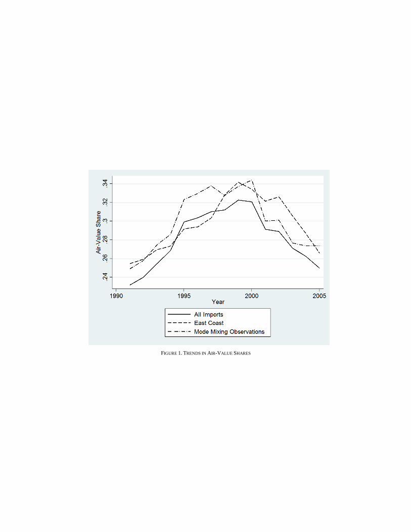
FIGURE 1. TRENDS IN AIR-VALUE SHARES

FIGURE 2. TRANSIT TIMES

TABLE 1—VARIATION IN AIR AND TRADE SHARES ACROSS COMMODITY GROUPS AND REGIONS
All Observations Mode Mixing Observations Median Air Premium
Group Share
Of Imports
Air
Share
Share of
Group Imports
Air
Share
Value Weight
All Imports: 1.00 .28 .75 .30 .05 6.46
Region:
Central America .03 .13 .60 .14 .03 3.25
South America .06 .12 .33 .21 .06 4.91
Europe .28 .39 .73 .38 .03 5.88
Asia .59 .27 .85 .28 .08 7.73
Australia/Oceania .01 .18 .48 .23 .04 6.00
Africa .04 .10 .15 .11 .08 5.42
End Use Categories:
Food .04 .04 .50 .06 .14 7.11
Industrial Supplies .23 .09 .36 .14 .07 8.90
Capital Goods .28 .52 .89 .52 .02 6.77
Automotive .12 .02 .92 .02 .06 7.58
Consumer Goods .30 .31 .86 .24 .06 5.20
Other .02 .80 .95 .80 -.01 7.70
Product Group:
Components .12 .41 .94 .39 .04 6.45
Fresh .01 .23 .49 .23 .17 5.55
Notes: Air Premium Value = = (1+air charge/air value)-(1+vessel charge/vessel value). Air Premium
Weight= =(air charge/air weight)/(vessel charge/vessel weight). A mode mixing observation is a
HS6 Exporter Year Coast observation that shows positive air and ocean values.
Source: Author calculations.
TABLE 2—REVENUE SPECIFICATION
(1) (2) (3) (4) (5)
Log Rel. Price -.078 -.074 .027 .009 .067 (.027)*** (.020)*** (.011)** (.009) (.014)***
Log Rel. Freight Cost -6.46 -5.823 -3.346 -2.673 -3.301
(.355)*** (.299)*** (.136)*** (.113)*** (.196)***
Transit Days .018 .045 .049 .060 .069
(.008)** (.010)*** (.014)*** (.017)*** (.018)***
Tau .003 .008 .015 .022 .021 (.001)** (.002)*** (.004)*** (.007)*** (.006)***
Fixed Effects None Exporter Exporter Exporter Coast +HS6 HS6 Differenced
Obs. 528977 528976 528721 513424 244530 R-Squared .121 .157 .356 .571 .159
Notes: Estimation of equation (8). Dependent Variable: log(air revenue/ocean revenue). Standard errors are robust and
clustered by exporter. Regressions include a constant.
*** Significant at the 1 percent level.
** Significant at the 5 percent level.
* Significant at the 10 percent level.
TABLE 3—REVENUE PER SHIPMENT SPECIFICATION
(1) (2) (3) (4) (5)
Log Rel. Price .037 .039 .038 .046 .070 (.005)*** (.004)*** (.006)** (.006)*** (.007)***
Log Rel. Freight Cost -1.861 -1.900 -1.584 -1.509 -1.554
(.094)*** (.081)*** (.077)*** (.075)*** (.095)***
Transit Days .008 .011 .008 .009 .010
(.002)*** (.002)*** (.002)*** (.002)*** (.002)***
Tau .004 .006 .005 .006 .006 (.0008)** (.001)*** (.001)*** (.001)*** (.001)***
Fixed Effects None Exporter Exporter Exporter Coast +HS6 HS6 Differenced
Obs. 528977 528976 528721 513424 244530 R-Squared .049 .057 .144 .351 .041
Notes: Estimation of equation (9). Dependent Variable: log(air revenue per shipment/ocean revenue per shipment).
Standard errors are robust and clustered by exporter. Regressions include a constant.
*** Significant at the 1 percent level.
** Significant at the 5 percent level.
* Significant at the 10 percent level.

TABLE 4—ROBUSTNESS CHECKS
(1) (2) (3) (4) (5) (6) (7) (8)
Dep. Variable
In Log:
Revenue Revenue
per Ship.
Revenue Revenue
per Ship.
Revenue Revenue
per Ship.
Revenue Revenue
per Ship.
Log Rel. .066 .070 .040 .064 -.042 .037 .038 .046 Price (.013)*** (.007)*** (.013)*** (.007)*** (.034) (.020)* (.012)*** (.007)***
Log Rel. -3.147 -1.532 -2.488 -1.242 -5.796 -2.763 -3.52 -1.619
Freight Cost
(.233)*** (.094)*** (.186)*** (.091)*** (.828)*** (.480)*** (.149)*** (.075)***
Transit .225 .032 .077 .012 .028 .007 .051 .009
Days (.038)*** (.005)*** (.020)*** (.002)*** (.0006)*** (.0003)*** (.015)*** (.002)***
Transit -.003 -.0005
Days Squared (.001)*** (.0001)***
Lag Dep. .648 .383
Variable (.004)*** (.004)***
Lag Freight 1.446 .776
Cost (.189)*** (.115)***
Tau .023 .007 .031 .010 015 005 (.005)*** (.0009)*** (.010)*** (.002)*** (.004)*** (.001)***
Fixed Coast
Differenced
Coast
Differenced
Coast
Differenced, IV Exporter
HS6 Year
Y
Effects
Obs. 244530 244530 321744 321744 110754 110754 505252 505252 R-Squared .21 .045 .153 .045 .353 .143
Notes: Standard errors in columns 1-4 are robust and clustered by exporter. The panel IV in columns 5 and 6 was
implemented using Stata’s xtivreg command which does not accommodate robust or clustered standard errors. The first
stage R2 for columns 5 and 6 are 0.43 and 0.42. In both IV regressions the instrument for the contemporaneous log relative freight rate is the second lag of the log relative freight rate. In both first stage regressions the instrument significantly
predicts the endogenous variable and the F test rejects the null hypothesis that the instruments don’t have a joint impact on
the endogenous variable. Regressions include a constant.
*** Significant at the 1 percent level.
** Significant at the 5 percent level.
* Significant at the 10 percent level.

TABLE 5—TIME COSTS BY END-USE GROUP
End Use: Foods
Beverages
Indust.
Supplies
Capital
Goods
Auto-
motive
Consumer
Goods
Log Revenue Specification: (1) (2) (3) (4) (5)
Log Rel. Price -.026 -.087 .072 .021 .016
(.034) (.011)*** (.016)*** (.030) (.013)
Log Rel. -1.522 -2.539 -3.132 -1.643 -2.969
Freight Cost (.208)*** (.125)*** (.319)*** (.241)*** (.126)***
Transit Days .048 .062 .063 .071 .058
(.010)*** (.013)*** (.014)*** (.015)*** (.023)**
Tau .031 .024 .020 .043 .019
(.008)*** (.006)*** (.006)*** (.011)*** (.008)**
Obs. 12065 143860 138079 18527 211155
R-Squared .61 .552 .568 .498 .562
Log Revenue per Shipment Specification:
(6) (7) (8) (9) (10)
Log Rel. Price .047 -.042 .117 .077 .046
(.028)* (.007)*** (.010)*** (.014)*** (.010)***
Log Rel. -.784 -1.647 -1.463 -.897 -1.619
Freight Cost (.103)*** (.079)*** (.188)*** (.094)*** (.094)***
Transit Days -.004 .007 .013 .012 .007
(.003) (.003)** (.004)*** (.002)*** (.003)**
Tau -.005 .004 .009 .013 .004
(.004) (.002)** (.002)*** (.003)*** (.002)**
Obs. 12065 143860 138079 18527 211155
R-Squared .452 .365 .348 .354 .324
Notes: Estimation of equations (8) and (9) by product subsamples. Standard errors are robust and clustered by exporter.
Regressions include a constant.
*** Significant at the 1 percent level.
** Significant at the 5 percent level.
* Significant at the 10 percent level.
TABLE 6—TIME COSTS BY PRODUCT CHARACTERISTICS
(1) (2) (3) (4)
Dependent Variable: Log Revenue Log Revenue per Shipment
Log Rel. Price .009 .009 .046 .046 (.009) (.009) (.006)*** (.006)***
Log Rel. Freight Cost -2.676 -2.676 -1.510 -1.510
(.114)*** (.114)*** (.075)*** (.075)***
Transit Days .060 .060 .008 .009
(.017)*** (.017)*** (.002)*** (.002)***
Component Share .122 -.054
(.094) (.036)
Component Share Days Days
-.002 .004
(.005) (.002)***
Fresh Share .697 .306
(.391)* (.137)**
Fresh Share Days
-.037 -.010
(.018)** (.007)
Tau (Share=0) .023 .023 .005 .006
(.007)*** (.007)*** (.001)*** (.001)***
Tau (Share=1) .022 .009 .008 -.0006
(.006)*** (.005) (.001)*** (.004)
Obs. 512012 512012 512012 512012 R-Squared .571 .571 .352 .352
Notes: Estimation of equations (8) and (9) by product characteristics. Standard errors are robust and clustered
by exporter. Regressions include a constant.
*** Significant at the 1 percent level.
** Significant at the 5 percent level.
* Significant at the 10 percent level.