Worcester Polytechnic InstituteDigitalCommons@WPI

Mechanical Engineering Faculty Publications Department of Mechanical Engineering

1-1-1985

Time Average Holography in Vibration AnalysisRyszard J. PryputniewiczWorcester Polytechnic Institute, rjp@wpi.edu

Follow this and additional works at: http://digitalcommons.wpi.edu/mechanicalengineering-pubsPart of the Mechanical Engineering Commons

This Article is brought to you for free and open access by the Department of Mechanical Engineering at DigitalCommons@WPI. It has been acceptedfor inclusion in Mechanical Engineering Faculty Publications by an authorized administrator of DigitalCommons@WPI.

Suggested CitationPryputniewicz, Ryszard J. (1985). Time Average Holography in Vibration Analysis. Optical Engineering, 24(5), 843-848.Retrieved from: http://digitalcommons.wpi.edu/mechanicalengineering-pubs/40

Time average holography in vibration analysis

Ryszard J. PryputniewiczWorcester Polytechnic InstituteDepartment of Mechanical EngineeringCenter for Holographic Studies

and Laser TechnologyWorcester, Massachusetts 01609

Abstract. This paper deals with the quantitative interpretation of time - averageholograms of vibrating objects. It is shown that the images obtained duringreconstruction of such holograms are modulated by a system of fringes de-scribed by the square of the zero -order Bessel function of the first kind. Aprocedure for quantitative interpretation of these fringes is describedand illustrated with examples. The experimental results, obtained directly fromthe time- average holograms, show good agreement with the exact solution ofthe differential equation of motion based on the beam theory andwith the modeshapes determined by the finite element modeling of the vibrating beam.

Subject terms: holographic interferometry; time -average holography; quantitative inter-pretation of holograms; vibrating objects; Jo fringes; finite element method; cantileverbeam; mode shape.

Optical Engineering 24(5), 843 -848 (September /October 1985).

CONTENTS1. Introduction2. Recording and reconstruction of time -average holograms3. Interpretation of time -average holograms4. Quantitative interpretation of time -average holograms of a canti-

lever beam5. Experimental setup6. Experimental results7. Conclusions8. References

1. INTRODUCTIONTransverse vibrations of beams are of primary interest in manyengineering applications. However, the conventional methods, bothanalytical and experimental, are rather limited when it comes tovibration analysis. In general, the analytical methods, including thefinite element techniques, require accurate knowledge of boundaryconditions and material properties. The experimental methods, onthe other hand, are invasive and frequently take into considerationonly a few points on the studied structure. The results obtained fromanalysis of these limited data are then "extrapolated" to predict thedynamic behavior of the structure. Also, as the vibration frequencyincreases, the corresponding displacement amplitude decreases, andmeasurement of vibrational characteristics of objects becomes diffi-cult when using conventional instrumentation. In 1965, however, themethod of hologram interferometry was invented ' and providedmeans for rapid, direct measurement of vibrational characteristics ofobjects in their full field of view.

Invited Paper HI-111 received Dec. 4, 1984; revised manuscript received Feb. 8, 1985;accepted for publication May 31, 1985; received by Managing Editor June 24, 1985.a 1985 Society of Photo -Optical Instrumentation Engineers.

Depending on the particular application, holographic interfero-grams may be recorded using one of the following techniques2: (i)double- exposure hologram interferometry, (ii) real -time holograminterferometry, (iii) time -average hologram interferometry. Thetime -average technique can be further subdivided into (i) strobo-scopic time -average hologram interferometry and (ii) "continuous"time -average hologram interferometry. Each of the above techniqueshas certain advantages over the others in specific vibration mea-surement applications. Regardless of the technique used, however,the fringe patterns observed during reconstructions of the hologramsrelate directly to changes in the object's position and/ or shape thatoccurred while the holograms were being recorded.3

Of particular interest to the discussions presented in this paper isthe technique of "continuous" time -average hologram interferome-try, which is popularly known as just time -average holography. Inthe following sections, the fundamental concept of time -averageholography is presented, interpretation of the resulting fringe pat-terns is outlined and illustrated with examples, and applications tothe finite element analysis of the vibrating beams are shown.

2. RECORDING AND RECONSTRUCTION OF TIME -AVERAGE HOLOGRAMSIn time -average hologram interferometry, a single holographicrecording of an object undergoing a cyclic vibration is made using,for example, the two -beam off -axis setup shown in Fig. 1. With the(continuous) exposure time long in comparison to one period of thevibration cycle, the hologram effectively records an ensemble ofimages corresponding to the time average of all positions of a vibrat-ing object. During reconstruction of such a hologram, interferenceoccurs between the entire ensemble of images, with the imagesrecorded near zero velocity (i.e., maximum displacement) contribut-

OPTICAL ENGINEERING / September /October 1985 / Vol. 24 No. 5 / 843

Time average holography in vibration analysis

Ryszard J. PryputniewiczWorcester Polytechnic Institute Department of Mechanical Engineering Center for Holographic Studies

and Laser Technology Worcester, Massachusetts 01609

Abstract. This paper deals with the quantitative interpretation of time-average holograms of vibrating objects. It is shown that the images obtained during reconstruction of such holograms are modulated by a system of fringes de­ scribed by the square of the zero-order Bessel function of the first kind. A procedure for quantitative interpretation of these fringes is described and illustrated with examples. The experimental results, obtained directly from the time-average holograms, show good agreement with the exact solution of the differential equation of motion based on the beam theory and with the mode shapes determined by the finite element modeling of the vibrating beam.

Subject terms: holographic interferometry; time-average holography; quantitative inter­ pretation of holograms; vibrating objects; J0 fringes; finite element method; cantilever beam; mode shape.

Optical Engineer ing 24(5)f 843-848 (September/October 1985).

CONTENTS1. Introduction2. Recording and reconstruction of time-average holograms3. Interpretation of time-average holograms4. Quantitative interpretation of time-average holograms of a canti­

lever beam5. Experimental setup6. Experimental results7. Conclusions8. References

1. INTRODUCTIONTransverse vibrations of beams are of primary interest in many engineering applications. However, the conventional methods, both analytical and experimental, are rather limited when it comes to vibration analysis. In general, the analytical methods, including the finite element techniques, require accurate knowledge of boundary conditions and material properties. The experimental methods, on the other hand, are invasive and frequently take into consideration only a few points on the studied structure. The results obtained from analysis of these limited data are then "extrapolated" to predict the dynamic behavior of the structure. Also, as the vibration frequency increases, the corresponding displacement amplitude decreases, and measurement of vibrational characteristics of objects becomes diffi­ cult when using conventional instrumentation. In 1965, however, the method of hologram interferometry was invented 1 and provided means for rapid, direct measurement of vibrational characteristics of objects in their full field of view.

Invited Paper HI-111 received Dec. 4, 1984; revised manuscript received Feb. 8, 1985; accepted for publication May 31, 1985; received by Managing Editor June 24, 1985. © 1985 Society of Photo-Optical Instrumentation Engineers.

Depending on the particular application, holographic interfero- grams may be recorded using one of the following techniques 2 : (i) double-exposure hologram interferometry, (ii) real-time hologram interferometry, (iii) time-average hologram interferometry. The time-average technique can be further subdivided into (i) strobo- scopic time-average hologram interferometry and (ii) "continuous" time-average hologram interferometry. Each of the above techniques has certain advantages over the others in specific vibration mea­ surement applications. Regardless of the technique used, however, the fringe patterns observed during reconstructions of the holograms relate directly to changes in the object's position and/ or shape that occurred while the holograms were being recorded. 3

Of particular interest to the discussions presented in this paper is the technique of "continuous" time-average hologram interferome­ try, which is popularly known as just time-average holography. In the following sections, the fundamental concept of time-average holography is presented, interpretation of the resulting fringe pat­ terns is outlined and illustrated with examples, and applications to the finite element analysis of the vibrating beams are shown.

2. RECORDING AND RECONSTRUCTION OF TIME- AVERAGE HOLOGRAMS

In time-average hologram interferometry, a single holographic recording of an object undergoing a cyclic vibration is made using, for example, the two-beam off-axis setup shown in Fig. 1. With the (continuous) exposure time long in comparison to one period of the vibration cycle, the hologram effectively records an ensemble of images corresponding to the time average of all positions of a vibrat­ ing object. During reconstruction of such a hologram, interference occurs between the entire ensemble of images, with the images recorded near zero velocity (i.e., maximum displacement) contribut-

OPTICAL ENGINEERING / September/October 1985 / Vol. 24 No. 5 / 843

Downloaded From: http://opticalengineering.spiedigitallibrary.org/ on 09/18/2012 Terms of Use: http://spiedl.org/terms

PRYPUTNIEWICZ

BEAMSPLITTER

LENS -PIN HOLEASSEMBLY

(2 PLACES)

HOLOGRAMMIRROR

(3 PLACES)

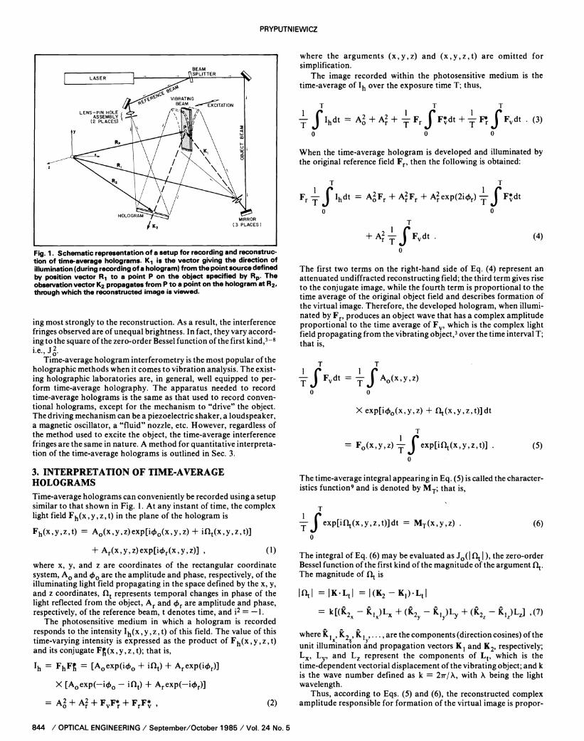
Fig. 1. Schematic representation of a setup for recording and reconstruction of time - average holograms. K1 is the vector giving the direction ofillumination (during recording of a hologram) from the point source definedby position vector R1 to a point P on the object specified by Rp. Theobservation vector K2 propagates from P to a point on the hologram at R2,through which the reconstructed image is viewed.

ing most strongly to the reconstruction. As a result, the interferencefringes observed are of unequal brightness. In fact, they vary accord-ing to the square of the zero -order Bessel function of the first kind,3 -9i.e., J.

Time -average hologram interferometry is the most popular of theholographic methods when it comes to vibration analysis. The exist-ing holographic laboratories are, in general, well equipped to per-form time -average holography. The apparatus needed to recordtime -average holograms is the same as that used to record conven-tional holograms, except for the mechanism to "drive" the object.The driving mechanism can be a piezoelectric shaker, a loudspeaker,a magnetic oscillator, a "fluid" nozzle, etc. However, regardless ofthe method used to excite the object, the time -average interferencefringes are the same in nature. A method for quantitative interpreta-tion of the time -average holograms is outlined in Sec. 3.

3. INTERPRETATION OF TIME -AVERAGEHOLOGRAMSTime -average holograms can conveniently be recorded using a setupsimilar to that shown in Fig. 1. At any instant of time, the complexlight field Fh(x , y , z , t) in the plane of the hologram is

Fh(x,y,z,t) = Ao(x,y,z)exp[i00(x,y,z) + iflt(x,y,z,t)]

+ Ar(x,y,z)eXp[i4r(x,y,z)] , (1)

where x, y, and z are coordinates of the rectangular coordinatesystem, Ao and 00 are the amplitude and phase, respectively, of theilluminating light field propagating in the space defined by the x, y,and z coordinates, flt represents temporal changes in phase of thelight reflected from the object, Ar and Or are amplitude and phase,respectively, of the reference beam, t denotes time, and i2 = -1.

The photosensitive medium in which a hologram is recordedresponds to the intensity Ih(x , y , z , t) of this field. The value of thistime -varying intensity is expressed as the product of Fh(x,y,z,t)and its conjugate Ft(x,y,z,t); that is,

Ih = FhFt = [Aoexp(i<po + iílt) + Arexp(icr)]

X [Aoexp( -i4o - Mt) + Arexp( -itr)]

= Aó + Ai + FvF . + FrF*v , (2)

844 / OPTICAL ENGINEERING / September /October 1985 / Vol. 24 No. 5

where the arguments (x,y,z) and (x,y,z,t) are omitted forsimplification.

The image recorded within the photosensitive medium is thetime -average of Ih over the exposure time T; thus,

¡T ¡T fT

,II-, J Ihdt = Aó + AT + .'-r Fr J F*dt -f- ,'-r F( Fvdt . (3)

o o o

When the time -average hologram is developed and illuminated bythe original reference field Fr, then the following is obtained:

Fr .l-r Ihdt = AFT + Aq.Fr + A; exp(2i0r) .1T. Ft,dt

o o

¡T+ Ai lI-. J Fvdt

0

(4)

The first two terms on the right -hand side of Eq. (4) represent anattenuated undiffracted reconstructing field; the third term gives riseto the conjugate image, while the fourth term is proportional to thetime average of the original object field and describes formation ofthe virtual image. Therefore, the developed hologram, when illumi-nated by Fr, produces an object wave that has a complex amplitudeproportional to the time average of Fv, which is the complex lightfield propagating from the vibrating object,3 over the time interval T;that is,

T

T1

Fvdt

o

T1

= T Ao(x,y,z)

X exp[ick(x,y,z) -- Sl(x,y,z,t)]dt

1

= Fo(x,y,z) T exp[iHt(x,y,z,t)]0

(5)

The time -average integral appearing in Eq. (5) is called the character-istics function9 and is denoted by MT; that is,

1T fexp[i1k(xy,zt)]dt = MT(x,y,z)o

(6)

The integral of Eq. (6) may be evaluated as Jo (I Sgt I ), the zero -orderBessel function of the first kind of the magnitude of the argument DI.The magnitude of DI is

Intl = IKLtI = I(K2 - Ki)LtI

= k[(K2x - Ki.)Lx + (K2Y - K1)Ly + (K22 - K,Z)Lz] ,(7)

where K i K2x, K i ..... are the components (direction cosines) of theunit illumination Ind propagation vectors Ki and K2, respectively;Lx, L. and Lx represent the components of Lt, which is thetime -dependent vectorial displacement of the vibrating object; and kis the wave number defined as k = 2a/ X, with X being the lightwavelength.

Thus, according to Eqs. (5) and (6), the reconstructed complexamplitude responsible for formation of the virtual image is propor-

PRYPUTNIEWICZ

BEAM _, \\SPLITTER

Fig. 1. Schematic representation of a setup for recording and reconstruc­ tion of time-average holograms. K 1 is the vector giving the direction of illumination (during recording of a hologram) from the point source defined by position vector RT to a point P on the object specified by Rp . The observation vector K2 propagates from P to a point on the hologram at R2, through which the reconstructed image is viewed.

ing most strongly to the reconstruction. As a result, the interference fringes observed are of unequal brightness. In fact, they vary accord­ ing to the square of the zero-order Bessel function of the first kind, 3-8 i.e.,J2.

Time-average hologram interferometry is the most popular of the holographic methods when it comes to vibration analysis. The exist­ ing holographic laboratories are, in general, well equipped to per­ form time-average holography. The apparatus needed to record time-average holograms is the same as that used to record conven­ tional holograms, except for the mechanism to "drive" the object. The driving mechanism can be a piezoelectric shaker, a loudspeaker, a magnetic oscillator, a "fluid" nozzle, etc. However, regardless of the method used to excite the object, the time-average interference fringes are the same in nature. A method for quantitative interpreta­ tion of the time-average holograms is outlined in Sec. 3.

3. INTERPRETATION OF TIME-AVERAGE HOLOGRAMSTime-average holograms can conveniently be recorded using a setup similar to that shown in Fig. 1. At any instant of time, the complex light field Fh(x,y,z,t) in the plane of the hologram is

Fh(x,y,z,t) = A0 (x,y,z)exp[i4>0(x,y,z) + iHt(x,y,z,t)]

+ Ar(x,y,z)exp[i<£r(x,y,z)] (1)

where x, y, and z are coordinates of the rectangular coordinate system, A0 and $0 are the amplitude and phase, respectively, of the illuminating light field propagating in the space defined by the x, y, and z coordinates, Ht represents temporal changes in phase of the light reflected from the object, Ar and <f> T are amplitude and phase, respectively, of the reference beam, t denotes time, and i2 = 1.

The photosensitive medium in which a hologram is recorded responds to the intensity Ih(x,y,z,t) of this field. The value of this time-varying intensity is expressed as the product of Fh(x,y,z,t) and its conjugate Fg(x,y,z,t); that is,

= [A0 exp(i00 + int) + Ar exp(i0r)]

(2)

X [A0 exp(-i«0 - iHt) + Ar exp(-i4>r)]

A 2 + A? + FVF* + FrF* ,

where the arguments (x,y,z) and (x,y,z,t) are omitted for simplification.

The image recorded within the photosensitive medium is the time-average of 1^ over the exposure time T; thus,

i i

= A*+A?+ y'Fr jF'dt+yF? J*Fv dt . (3)

When the time-average hologram is developed and illuminated by the original reference field Fr, then the following is obtained:

Fr Y J\dt = A2pr + A2r Fr + A?exp(2i4>r) y § F*dt

(4)

The first two terms on the right-hand side of Eq. (4) represent an attenuated undiffracted reconstructing field; the third term gives rise to the conjugate image, while the fourth term is proportional to the time average of the original object field and describes formation of the virtual image. Therefore, the developed hologram, when illumi­ nated by Fr, produces an object wave that has a complex amplitude proportional to the time average of Fv, which is the complex light field propagating from the vibrating object, 3 over the time interval T; that is,

X exp[i</>0 (x,y,z) +

T

= F0 (x,y,z) Y J exp[int(x,y,z,t)] . (5)

The time-average integral appearing in Eq. (5) is called the character­ istics function 9 and is denoted by MT; that is,

i

Y J= MT (x,y,z) . (6)

The integral of Eq. (6) may be evaluated as J0 (| (\ \ ), the zero-order Bessel function of the first kind of the magnitude of the argument f^. The magnitude of fy is

,(7)

=|K-Lt | =|(K2 -K,)-Lt |

= k[(K2x - K lx)Lx + (K2y - K ly)Ly

where Kj ,K2 ,Kj ,..., are the components (direction cosines) of the unit illumination and propagation vectors Kj and K 2, respectively; Lx , Ly, and Lz represent the components of L t , which is the time-dependent vectorial displacement of the vibrating object; and k is the wave number defined as k = 27T/X, with X being the light wavelength.

Thus, according to Eqs. (5) and (6), the reconstructed complex amplitude responsible for formation of the virtual image is propor-

844 / OPTICAL ENGINEERING / September/October 1985 / Vol. 24 No. 5

Downloaded From: http://opticalengineering.spiedigitallibrary.org/ on 09/18/2012 Terms of Use: http://spiedl.org/terms

TIME AVERAGE HOLOGRAPHY IN VIBRATION ANALYSIS

tional to Fo. MT, while the corresponding intensity Ih(x, y, z) of thereconstructed image is

Iim(x,Y,z) = [F0(x,y,z)]2 [MT(x,y,z)]2 = AoJo(Iflto (8)

Equation (8) shows that the virtual image obtained during recon-struction of a time -average hologram is modulated by a system offringes described by the square of the zero -order Bessel function ofthe first kind. Thus, for nontrivial value of Ao, centers of the darkfringes will be located at those points on the object's surface whereJo(I fZt I ) equals zero.

The images formed during reconstruction of time -average holo-grams of cosinusoidal motions are modulated according to the varia-tions of J. The Jo fringes differ from the cosinusoidal fringesobtained in conventional double- exposure hologram interferometry.One of these differences is that the zero -order fringe is much brighterthan the higher order Jo fringes, while all cosinusoidal fringes,regardless of their order, show equal brightness. Furthermore, thezero -order fringes represent the stationary points on the vibratingobject and thus allow easy identification of nodes. The brightness ofother fringes, as well as their spacing, decreases with increasing fringeorder and can be directly related to the mode shapes.

Representative application of Eqs. (1) to (8) in quantitative inter-pretation of transverse vibrations of a cantilever beam is discussed inSec. 4.

4. QUANTITATIVE INTERPRETATION OF TIME -AVERAGE HOLOGRAMS OF A CANTILEVER BEAMIn this representative example, the cantilever beam was rigidly fixedat the lower end, while its upper end was free. Cosinusoidal excita-tion was applied to the free end by means of a loudspeaker. Theexcitation was always set in such a way that the beam motion was inthe direction parallel to the z -axis of the rectangular coordinatesystem. That is, for this case, Eq. (7) became

IHtI = k(K2Z- R1)Lz , (9)

wherefrom the vibration amplitude Lz was determined to be

LZ =27r(K2 - K,) IRt

(10)

Z Z

The goal of the analysis was to determine Lz as a function of positionon the vibrating beam, which gave the mode shape. However, beforethis could be done, the quantity (K2Z -K iZ) has to be evaluated forevery point of interest on the vibrating object.

For the case of retroreflective illumination and observation,parallel to the z -axis, the quantity (K2Z - KIZ) has the maximumvalue of 2. For any other geometry, where the directions of illumina-tion and observation are not parallel to the z -axis, the quantity(K2 - KI ) will always be less than 2. Its actual magnitude willdepénd on The magnitudes of angles that the directions of Ki and K2make with the direction of L. That is, for every case when directionsof illumination and observation deviate from being parallel to thedirection of motion, the Lz, as computed from Eq. (10), will alwaysbe greater than for the retroreflective case for the same order of the Jofringe.3

5. EXPERIMENTAL SETUPThe cantilever beam used in this study was rigidly fixed at the bottomand free at the top. Its length was 160 mm (6.3 in.); it was 28.58 mm(1.125 in.) wide and 3.18 mm (0.125 in.) thick. The cantilever beam,made of 6061 -T6 aluminum, was excited acoustically at its free end.The origin of the right- handed coordinate system was located at thefixed end of the cantilever beam with the positive z -axis pointingtoward the hologram. The time -average holograms of the vibratingcantilever beam were recorded using the experimental setup shown

o TIME -AVERAGE HOLOGRAMS

BEAM THEORY

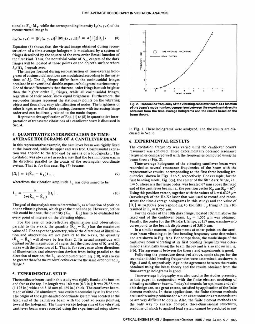
Fig. 2. Resonance frequency of the vibrating cantilever beam as a functionof the beam's mode number: comparison between the experimental resultsobtained from the time- average holograms and the results based on thebeam theory.

in Fig. 1. These holograms were analyzed, and the results are dis-cussed in Sec. 6.

6. EXPERIMENTAL RESULTSThe excitation frequency was varied until the cantilever beam'sresonance was achieved. These experimentally obtained resonancefrequencies compared well with the frequencies computed using thebeam theory (Fig. 2).

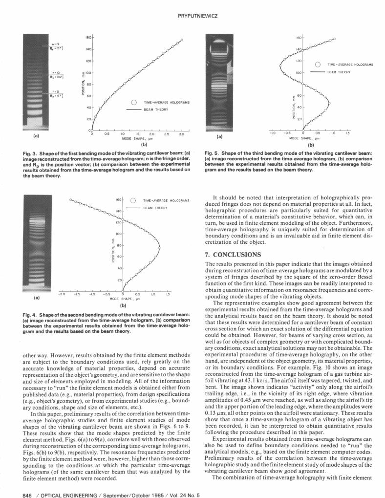
Time- average holograms of the vibrating cantilever beam wererecorded at several resonance frequencies of the beam with therepresentative results, corresponding to the first three bending fre-quencies, shown in Figs. 3 to 5, respectively. For example, for thefirst bending mode, Fig. 3(a), the center of the fifth dark fringe, i.e.,n = 5, where n is the fringe order, was located 67 mm above the fixedend of the cantilever beam; i.e., the position vector Rp was Rp = 67 j.Using this position vector, together with the values of X = 0.6328µm(wavelength of the He -Ne laser that was used to record and recon-struct the time -average holograms in this study) and the value ofIntl = 14.93092 (corresponding to the fifth Jo fringe),3 Eq. (10)resulted in Lz = 0.757 µm.

For the center of the 10th dark fringe, located 102 mm above thefixed end of the cantilever beam, Lz = 1.557 µm was obtained.Finally, the center for the 19th dark fringe, at 157 mm, was shown tocorrespond to the beam's displacement of 3.010 µm.

In a similar manner, displacements at other points on the canti-lever beam vibrating at its first bending frequency were determinedand are shown in Fig. 3(b). For comparison, the mode shape of thecantilever beam vibrating at its first bending frequency was deter-mined analytically using the beam theory and is also shown in Fig.3(b). The agreement between the theory and experiments is good.

Following the procedure described above, mode shapes for thesecond and third bending frequencies were determined, as shown inFigs. 4 and 5, respectively. Again the agreement between the resultsobtained using the beam theory and the results obtained from thetime -average holograms is good.

Time -average holography was also used in the studies presentedin this paper in conjunction with the finite element modeling ofvibrating cantilever beams. Today's demands for optimum and reli-able design are, to a great extent, satisfied by application of the finiteelement methods. In these applications, the finite element methodsare used to solve problems for which exact solutions are nonexistentor are very difficult to obtain. Also, the finite element methods arethe only way to analyze complex three -dimensional structures,response of which to applied load system cannot be predicted in any

OPTICAL ENGINEERING / September /October 1985 / Vol. 24 No. 5 / 845

TIME AVERAGE HOLOGRAPHY IN VIBRATION ANALYSIS

0 - IT* T, while the corresponding intensity I h (x,y,z) of thetionaltoF 0 -M reconstructed image is

I im(x,y,z) - [F 0 (x,y,z)]2[MT(x,y,z)] 2 - (8)

Equation (8) shows that the virtual image obtained during recon­ struction of a time-average hologram is modulated by a system of fringes described by the square of the zero-order Bessel function of the first kind. Thus, for nontrivial value of A Q , centers of the dark fringes will be located at those points on the object's surface where J0(|nt |)equalszero.

The images formed during reconstruction of time-average holo­ grams of cosinusoidal motions are modulated according to the varia­ tions of J 2 . The J0 fringes differ from the cosinusoidal fringes obtained in conventional double-exposure hologram interferometry. One of these differences is that the zero-order fringe is much brighter than the higher order JQ fringes, while all cosinusoidal fringes, regardless of their order, show equal brightness. Furthermore, the zero-order fringes represent the stationary points on the vibrating object and thus allow easy identification of nodes. The brightness of other fringes, as well as their spacing, decreases with increasing fringe order and can be directly related to the mode shapes.

Representative application of Eqs. ( 1 ) to (8) in quantitative inter­ pretation of transverse vibrations of a cantilever beam is discussed in Sec. 4.

4. QUANTITATIVE INTERPRETATION OF TIME- AVERAGE HOLOGRAMS OF A CANTILEVER BEAMIn this representative example, the cantilever beam was rigidly fixed at the lower end, while its upper end was free. Cosinusoidal excita­ tion was applied to the free end by means of a loudspeaker. The excitation was always set in such a way that the beam motion was in the direction parallel to the z-axis of the rectangular coordinate system. That is, for this case, Eq. (7) became

|nt | =

wherefrom the vibration amplitude L was determined to be

2jr(K, - K.-|ftt l

(9)

(10)

The goal of the analysis was to determine Lz as a function of position on the vibrating beam, which gavejthe mode shape. However, before this could be done, the quantity (K2z KI Z) has to be evaluated for every point of interest on the vibrating object.

For the case of retroreflective illumination and observation, parallel to the z-axis, the quantity (K2z KI Z) has the maximum value of 2. For any other geometry, where the directions of illumina­ tion and observation are not parallel to the z-axis, the quantity (K 2 Kj ) will always be less than 2. Its actual magnitude will depend onfaie magnitudes of angles that the directions of Kj and K 2 make with the direction of L. That is, for every case when directions of illumination and observation deviate from being parallel to the direction of motion, the LZ , as computed from Eq. (10), will always be greater than for the retroreflective case for the same order of the J Q fringe. 3

5. EXPERIMENTAL SETUPThe cantilever beam used in this study was rigidly fixed at the bottom and free at the top. Its length was 160 mm (6.3 in.); it was 28.58 mm (1.125 in.) wide and 3.18 mm (0.125 in.) thick. The cantilever beam, made of 6061-T6 aluminum, was excited acoustically at its free end. The origin of the right-handed coordinate system was located at the fixed end of the cantilever beam with the positive z-axis pointing toward the hologram. The time-average holograms of the vibrating cantilever beam were recorded using the experimental setup shown

TIME-AVERAGE HOLOGRAMS

BEAM THEORY

345

MODE NUMBER

Fig. 2. Resonance frequency of the vibrating cantilever beam as a function of the beam's mode number: comparison between the experimental results obtained from the time-average holograms and the results based on the beam theory.

in Fig. 1. These holograms were analyzed, and the results are dis­ cussed in Sec. 6.

6. EXPERIMENTAL RESULTSThe excitation frequency was varied until the cantilever beam's resonance was achieved. These experimentally obtained resonance frequencies compared well with the frequencies computed using the beam theory (Fig. 2).

Time-average holograms of the vibrating cantilever beam were recorded at several resonance frequencies of the beam with the representative results, corresponding to the first three bending fre­ quencies, shown in Figs. 3 to 5, respectively. For example, for the first bending mode, Fig. 3(a), the center of the fifth dark fringe, i.e., n = 5, where n is the fringe order, was located 67 mm above the fixed end of the cantilever beam; i.e., the position vector R p was R p = 67 j. Using this position vector, together with the values of A = 0.6328 pm (wavelength of the He-Ne laser that was used to record and recon­ struct the time-average holograms in this study) and the value of |nt | = 14.93092 (corresponding to the fifth J0 fringe), 3 Eq. (10) resulted in LZ = 0.757 jum.

For the center of the 10th dark fringe, located 102 mm above the fixed end of the cantilever beam, LZ = 1.557 jitm was obtained. Finally, the center for the 19th dark fringe, at 157 mm, was shown to correspond to the beam's displacement of 3.010 /zm.

In a similar manner, displacements at other points on the canti­ lever beam vibrating at its first bending frequency were determined and are shown in Fig. 3(b). For comparison, the mode shape of the cantilever beam vibrating at its first bending frequency was deter­ mined analytically using the beam theory and is also shown in Fig. 3(b). The agreement between the theory and experiments is good.

Following the procedure described above, mode shapes for the second and third bending frequencies were determined, as shown in Figs. 4 and 5, respectively. Again the agreement between the results obtained using the beam theory and the results obtained from the time-average holograms is good.

Time-average holography was also used in the studies presented in this paper in conjunction with the finite element modeling of vibrating cantilever beams. Today's demands for optimum and reli­ able design are, to a great extent, satisfied by application of the finite element methods. In these applications, the finite element methods are used to solve problems for which exact solutions are nonexistent or are very difficult to obtain. Also, the finite element methods are the only way to analyze complex three-dimensional structures, response of which to applied load system cannot be predicted in any

OPTICAL ENGINEERING / September/October 1985 / Vol. 24 No. 5 / 845

Downloaded From: http://opticalengineering.spiedigitallibrary.org/ on 09/18/2012 Terms of Use: http://spiedl.org/terms

(a)

160

140

120

E 100

2O 80F

2 o

40

o

PRYPUTNIEWICZ

O TIME-AVERAGE HOLOGRAMS

BEAM THEORY

as LO 1.5 2.0MODE SHAPE, ym

(b)

2.5 3.0

Fig. 3. Shape of the first bending mode of the vibrating cantilever beam: (a)image reconstructed from the time -average hologram; n is the fringe order,and Rp is the position vector; (b) comparison between the experimentalresults obtained from the time -average hologram and the results based onthe beam theory.

(a)

160

190

TIME- AVERAGE HOLOGRAMS

BEAM THEORY

120

100

EE

80ó

t75 60o

40

20

-2.0 .5 .O -0.5 0 0.5MODE SHAPE, Vm

(b)

Fig. 4. Shape of the second bending mode of the vibrating cantilever beam:(a) image reconstructed from the time - average hologram, (b) comparisonbetween the experimental results obtained from the time - average holo-gram and the results based on the beam theory.

_I -I .0 1.5

other way. However, results obtained by the finite element methodsare subject to the boundary conditions used, rely greatly on theaccurate knowledge of material properties, depend on accuraterepresentation of the object's geometry, and are sensitive to the shapeand size of elements employed in modeling. All of the informationnecessary to "run" the finite element models is obtained either frompublished data (e.g., material properties), from design specifications(e.g., object's geometry), or from experimental studies (e.g., bound-ary conditions, shape and size of elements, etc.).

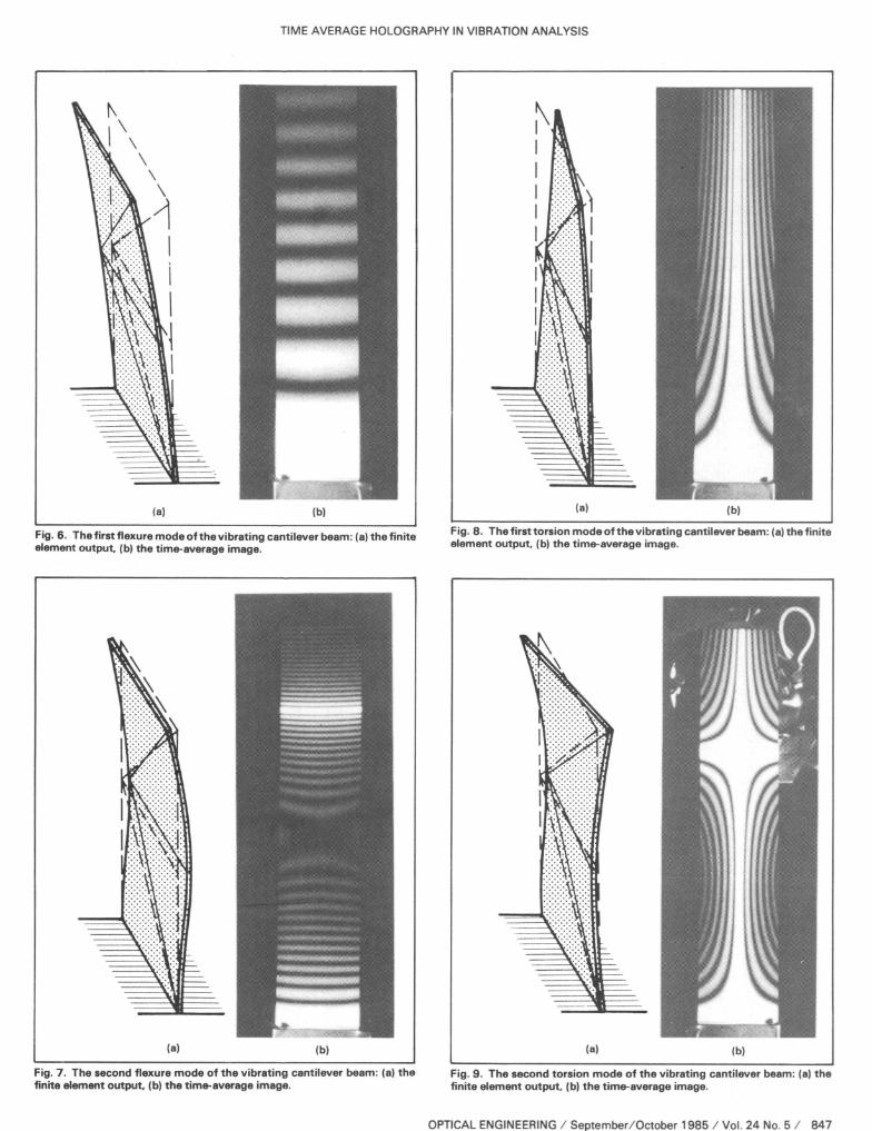
In this paper, preliminary results of the correlation between time -average holographic studies and finite element studies of modeshapes of the vibrating cantilever beam are shown in Figs. 6 to 9.These results show that the mode shapes predicted by the finiteelement method, Figs. 6(a) to 9(a), correlate well with those observedduring reconstruction of the corresponding time -average holograms,Figs. 6(b) to 9(b), respectively. The resonance frequencies predictedby the finite element method were, however, higher than those corre-sponding to the conditions at which the particular time -averageholograms (of the same cantilever beam that was analyzed by thefinite element method) were recorded.

846 / OPTICAL ENGINEERING / September /October 1985 / Vol. 24 No. 5

(a)

1601-

140

O TIME - AVERAGE HOLOGRAMS

BEAM THEORY

60E

40

on

-1.0 -0.5 0 05MODE SHAPE, pm

(b)

Fig. 5. Shape of the third bending mode of the vibrating cantilever beam:(a) image reconstructed from the time - average hologram, (b) comparisonbetween the experimental results obtained from the time -average holo-gram and the results based on the beam theory.

It should be noted that interpretation of holographically pro-duced fringes does not depend on material properties at all. In fact,holographic procedures are particularly suited for quantitativedetermination of a material's constitutive behavior, which can, inturn, be used in finite element modeling of the object. Furthermore,time -average holography is uniquely suited for determination ofboundary conditions and is an invaluable aid in finite element dis-cretization of the object.

7. CONCLUSIONSThe results presented in this paper indicate that the images obtainedduring reconstruction of time -average holograms are modulated by asystem of fringes described by the square of the zero -order Besselfunction of the first kind. These images can be readily interpreted toobtain quantitative information on resonance frequencies and corre-sponding mode shapes of the vibrating objects.

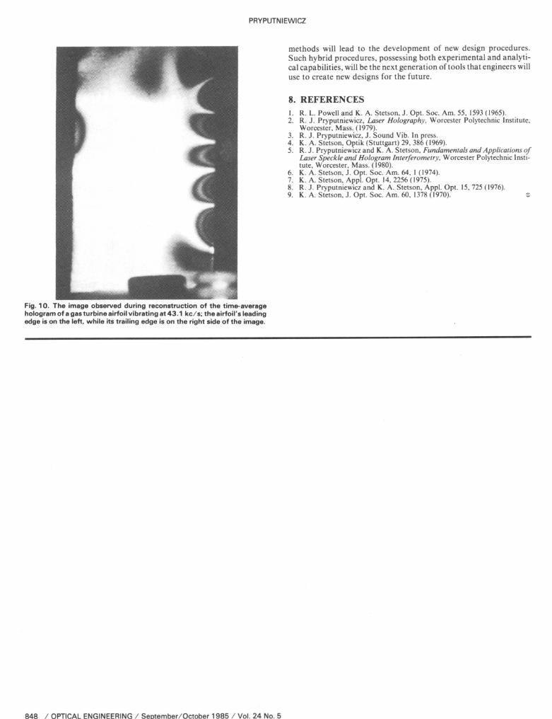
The representative examples show good agreement between theexperimental results obtained from the time -average holograms andthe analytical results based on the beam theory. It should be notedthat these results were determined for a cantilever beam of constantcross section for which an exact solution of the differential equationcould be obtained. However, for beams of varying cross section, aswell as for objects of complex geometry or with complicated bound-ary conditions, exact analytical solutions may not be obtainable. Theexperimental procedures of time- average holography, on the otherhand, are independent of the object geometry, its material properties,or its boundary conditions. For example, Fig. 10 shows an imagereconstructed from the time -average hologram of a gas turbine air-foil vibrating at 43.1 kc/ s. The airfoil itself was tapered, twisted, andbent. The image shown indicates "activity" only along the airfoil'strailing edge, i.e., in the vicinity of its right edge, where vibrationamplitudes of 0.45 µm were reached, as well as along the airfoil's tipand the upper portion of the leading edge, where the amplitudes were0.13µm; all other points on the airfoil were stationary. These resultsshow that once a time -average hologram of a vibrating object hasbeen recorded, it can be interpreted to obtain quantitative resultsfollowing the procedure described in this paper.

Experimental results obtained from time -average holograms canalso be used to define boundary conditions needed to "run" theanalytical models, e.g., based on the finite element computer codes.Preliminary results of the correlation between the time -averageholographic study and the finite element study of mode shapes of thevibrating cantilever beam show good agreement.

The combination of time -average holography with finite element

PRYPUTNIEWICZ

TIME-AVERAGE HOLOGRAMS

BEAM THEORY

1.0 1.5 2.0

MODE SHAPE, ym

(b)

Fig. 3. Shape of the first bending mode of the vibrating cantilever beam: (a) image reconstructed from the time-average hologram; n is the fringe order, and R p is the position vector; (b) comparison between the experimental results obtained from the time-average hologram and the results based on the beam theory.

Q TIME-AVERAGE HOLOGRAMS

BEAM THEORY

-1.0 -0.5 0 0.5 1.0 1.5

MODE SHAPE, pm

(b)

Fig. 5. Shape of the third bending mode of the vibrating cantilever beam: (a) image reconstructed from the time-average hologram, (b) comparison between the experimental results obtained from the time-average holo­ gram and the results based on the beam theory.

Q TIME-AVERAGE HOLOGRAMS

BEAM THEORY

Fig. 4. Shape of the second bending mode of the vibrating cantilever beam: (a) image reconstructed from the time-average hologram, (b) comparison between the experimental results obtained from the time-average holo­ gram and the results based on the beam theory.

other way. However, results obtained by the finite element methods are subject to the boundary conditions used, rely greatly on the accurate knowledge of material properties, depend on accurate representation of the object's geometry, and are sensitive to the shape and size of elements employed in modeling. All of the information necessary to "run" the finite element models is obtained either from published data (e.g., material properties), from design specifications (e.g., object's geometry), or from experimental studies (e.g., bound­ ary conditions, shape and size of elements, etc.).

In this paper, preliminary results of the correlation between time- average holographic studies and finite element studies of mode shapes of the vibrating cantilever beam are shown in Figs. 6 to 9. These results show that the mode shapes predicted by the finite element method, Figs. 6(a) to 9(a), correlate well with those observed during reconstruction of the corresponding time-average holograms, Figs. 6(b) to 9(b), respectively. The resonance frequencies predicted by the finite element method were, however, higher than those corre­ sponding to the conditions at which the particular time-average holograms (of the same cantilever beam that was analyzed by the finite element method) were recorded.

It should be noted that interpretation of holographically pro­ duced fringes does not depend on material properties at all. In fact, holographic procedures are particularly suited for quantitative determination of a material's constitutive behavior, which can, in turn, be used in finite element modeling of the object. Furthermore, time-average holography is uniquely suited for determination of boundary conditions and is an invaluable aid in finite element dis­ cretization of the object.

7. CONCLUSIONSThe results presented in this paper indicate that the images obtained during reconstruction of time-average holograms are modulated by a system, of fringes described by the square of the zero-order Bessel function of the first kind. These images can be readily interpreted to obtain quantitative information on resonance frequencies and corre­ sponding mode shapes of the vibrating objects.

The representative examples show good agreement between the experimental results obtained from the time-average holograms and the analytical results based on the beam theory. It should be noted that these results were determined for a cantilever beam of constant cross section for which an exact solution of the differential equation could be obtained. However, for beams of varying cross section, as well as for objects of complex geometry or with complicated bound­ ary conditions, exact analytical solutions may not be obtainable. The experimental procedures of time-average holography, on the other hand, are independent of the object geometry, its material properties, or its boundary conditions. For example, Fig. 10 shows an image reconstructed from the time-average hologram of a gas turbine air­ foil vibrating at 43.1 kc/ s. The airfoil itself was tapered, twisted, and bent. The image shown indicates "activity" only along the airfoil's trailing edge, i.e., in the vicinity of its right edge, where vibration amplitudes of 0.45 urn were reached, as well as along the airfoil's tip and the upper portion of the leading edge, where the amplitudes were 0.13 jitm; all other points on the airfoil were stationary. These results show that once a time-average hologram of a vibrating object has been recorded, it can be interpreted to obtain quantitative results following the procedure described in this paper.

Experimental results obtained from time-average holograms can also be used to define boundary conditions needed to "run" the analytical models, e.g., based on the finite element computer codes. Preliminary results of the correlation between the time-average holographic study and the finite element study of mode shapes of the vibrating cantilever beam show good agreement.

The combination of time-average holography with finite element

846 / OPTICAL ENGINEERING / September/October 1985 / Vol. 24 No. 5Downloaded From: http://opticalengineering.spiedigitallibrary.org/ on 09/18/2012 Terms of Use: http://spiedl.org/terms

TIME AVERAGE HOLOGRAPHY IN VIBRATION ANALYSIS

Fig. 6. The first flexure mode of the vibrating cantilever beam: (a) the finiteelement output, (b) the time -average image.

Fig. 7. The second flexure mode of the vibrating cantilever beam: (a) thefinite element output, (b) the time -average image.

(a) (b)

Fig. 8. The first torsion mode of the vibrating cantilever beam: (a) the finiteelement output, (b) the time- average image.

Fig. 9. The second torsion mode of the vibrating cantilever beam: (a) thefinite element output, (b) the time -average image.

OPTICAL ENGINEERING / September /October 1985 / Vol. 24 No. 5 / 847

TIME AVERAGE HOLOGRAPHY IN VIBRATION ANALYSIS

(b)

Fig. 6. The first I lexure mode of the vibrating cantilever beam: (a) the finite element output, (b) the time-average image.

Fig. 8. The first torsion mode of the vibrating cantilever beam: (a) the finite element output, (b) the time-average image.

Fig. 7. The second flexure mode of the vibrating cantilever beam: (a) the finite element output (b) the time-average image.

Fig. 9. The second torsion mode of the vibrating cantilever beam: (a) the finite element output, (b) the time-average image.

OPTICAL ENGINEERING / September/October 1985 / Vol. 24 No. 5 / 847Downloaded From: http://opticalengineering.spiedigitallibrary.org/ on 09/18/2012 Terms of Use: http://spiedl.org/terms

PRYPUTNIEWICZ

Fig. 10. The image observed during reconstruction of the time -averagehologram of a gas turbine airfoil vibrating at 43.1 kc /s; the airfoil's leadingedge is on the left, while its trailing edge is on the right side of the image.

methods will lead to the development of new design procedures.Such hybrid procedures, possessing both experimental and analyti-cal capabilities, will be the next generation of tools that engineers willuse to create new designs for the future.

8. REFERENCESI. R. L. Powell and K. A. Stetson, J. Opt. Soc. Am. 55, 1593 (1965).2. R. J. Pryputniewicz, Laser Holography, Worcester Polytechnic Institute,

Worcester, Mass. (1979).3. R. J. Pryputniewicz, J. Sound Vib. In press.4. K. A. Stetson, Optik (Stuttgart) 29, 386 (1969).5. R. J. Pryputniewicz and K. A. Stetson, Fundamentals and Applications of

Laser Speckle and Hologram Interferometry, Worcester Polytechnic Insti-tute, Worcester, Mass. (1980).

6. K. A. Stetson, J. Opt. Soc. Am. 64, I (1974).7. K. A. Stetson, Appt. Opt. 14, 2256 (1975).8. R. J. Pryputniewicz and K. A. Stetson, Appl. Opt. 15, 725 (1976).9. K. A. Stetson, J. Opt. Soc. Am. 60, 1378 (1970).

848 / OPTICAL ENGINEERING / September /October 1985 / Vol. 24 No. 5

PRYPUTNIEWICZ

methods will lead to the development of new design procedures, Such hybrid procedures, possessing both experimental and analyti­ cal capabilities, will be the next generation of tools that engineers will use to create new designs for the future.

8. REFERENCES1. R. L, Powell and K. A. Stetson, J. Opt. Soc. Am. 55, 1593 (1965).2. R. J. Pryputniewicz, Laser Holography, Worcester Polytechnic Institute,

Worcester, Mass. (1979).3. R. J. Pryputniewicz, J. Sound Vib. In press.4. K. A. Stetson, Optik (Stuttgart) 29, 386 (1969).5. R. J. Pryputniewicz and K. A. Stetson, Fundamentals and Applications of

Laser Speckle and Hologram Interferometry, Worcester Polytechnic Insti­ tute, Worcester, Mass. (1980).

6. K. A. Stetson, J. Opt. Soc. Am. 64, 1 (1974).7. K. A. Stetson, Appl. Opt. 14, 2256 (1975).8. R. J. Pryputniewicz and K. A. Stetson, Appl. Opt. 15, 725 (1976).9. K. A. Stetson, J. Opt. Soc. Am. 60, 1378 (1970). 3

Fig. 10. Trie image observed during reconstruction of the time-average hologram of a gas turbine airfoil vibrating at 43.1 kc/s; the airfoil's leading edge is on the left, while its trailing edge is on the right side of the image.

848 / OPTICAL ENGINEERING / September/October 1985 / Vol. 24 No. 5Downloaded From: http://opticalengineering.spiedigitallibrary.org/ on 09/18/2012 Terms of Use: http://spiedl.org/terms