Embed Size (px)
Citation preview

Time Dependent Density Functional TheoryAn introduction
Francesco Sottile
LSI, Ecole Polytechnique, PalaiseauEuropean Theoretical Spectroscopy Facility (ETSF)
Palaiseau, 7 February 2012
Francesco Sottile (ETSF) Time Dependent Density Functional Theory Palaiseau, 7 February 2012 1 / 32

Outline
1 Introduction: why TD-DFT ?
2 (Just) A bit of Formalism - The Boring PartTDDFT: the FoundationLinear Response Formalism
3 TDDFT in practice:The ALDA: Achievements and ShortcomingsThe Quest for the Holy FunctionalNew Frontiers
4 Perspectives and Resources
Francesco Sottile (ETSF) Time Dependent Density Functional Theory Palaiseau, 7 February 2012 2 / 32

Outline
1 Introduction: why TD-DFT ?
2 (Just) A bit of Formalism - The Boring PartTDDFT: the FoundationLinear Response Formalism
3 TDDFT in practice:The ALDA: Achievements and ShortcomingsThe Quest for the Holy FunctionalNew Frontiers
4 Perspectives and Resources
Francesco Sottile (ETSF) Time Dependent Density Functional Theory Palaiseau, 7 February 2012 3 / 32
Outline
1 Introduction: why TD-DFT ?
2 (Just) A bit of Formalism - The Boring PartTDDFT: the FoundationLinear Response Formalism
3 TDDFT in practice:The ALDA: Achievements and ShortcomingsThe Quest for the Holy FunctionalNew Frontiers
4 Perspectives and Resources
Francesco Sottile (ETSF) Time Dependent Density Functional Theory Palaiseau, 7 February 2012 4 / 32
Outline
1 Introduction: why TD-DFT ?
2 (Just) A bit of Formalism - The Boring PartTDDFT: the FoundationLinear Response Formalism
3 TDDFT in practice:The ALDA: Achievements and ShortcomingsThe Quest for the Holy FunctionalNew Frontiers
4 Perspectives and Resources
Francesco Sottile (ETSF) Time Dependent Density Functional Theory Palaiseau, 7 February 2012 5 / 32
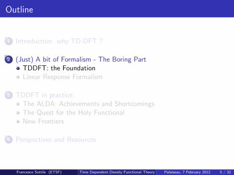
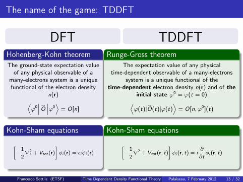
The name of the game: TDDFT
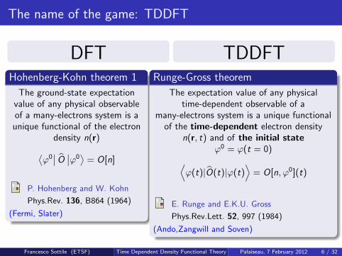
DFT TDDFTHohenberg-Kohn theorem 1
The ground-state expectationvalue of any physical observableof a many-electrons system is aunique functional of the electron
density n(r)⟨ϕ0∣∣ O ∣∣ϕ0
⟩= O[n]
P. Hohenberg and W. Kohn
Phys.Rev. 136, B864 (1964)
(Fermi, Slater)
Runge-Gross theorem
The expectation value of any physicaltime-dependent observable of a
many-electrons system is a unique functionalof the time-dependent electron density
n(r, t) and of the initial stateϕ0 = ϕ(t = 0)⟨
ϕ(t)|O(t)|ϕ(t)⟩
= O[n, ϕ0](t)
E. Runge and E.K.U. Gross
Phys.Rev.Lett. 52, 997 (1984)
(Ando,Zangwill and Soven)
Francesco Sottile (ETSF) Time Dependent Density Functional Theory Palaiseau, 7 February 2012 6 / 32
The name of the game: TDDFT
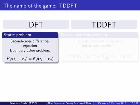
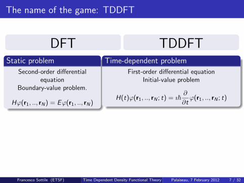
DFT TDDFTStatic problem
Second-order differentialequation
Boundary-value problem.
Hϕ(r1, .., rN) = Eϕ(r1, .., rN)
Time-dependent problem
First-order differential equationInitial-value problem
H(t)ϕ(r1, .., rN ; t) = ı~∂
∂tϕ(r1, .., rN ; t)
Francesco Sottile (ETSF) Time Dependent Density Functional Theory Palaiseau, 7 February 2012 7 / 32
The name of the game: TDDFT
DFT TDDFTStatic problem
Second-order differentialequation
Boundary-value problem.
Hϕ(r1, .., rN) = Eϕ(r1, .., rN)
Time-dependent problem
First-order differential equationInitial-value problem
H(t)ϕ(r1, .., rN ; t) = ı~∂
∂tϕ(r1, .., rN ; t)
Francesco Sottile (ETSF) Time Dependent Density Functional Theory Palaiseau, 7 February 2012 7 / 32

The name of the game: TDDFT
Runge-Gross theorem
The expectation value of any physicaltime-dependent observable of a many-electrons
system is a unique functional of thetime-dependent electron density n(r, t) and of
the initial state ϕ0 = ϕ(t = 0)⟨ϕ(t)|O(t)|ϕ(t)
⟩= O[n, ϕ0](t)
E. Runge and E.K.U. Gross
Phys.Rev.Lett. 52, 997 (1984)
Francesco Sottile (ETSF) Time Dependent Density Functional Theory Palaiseau, 7 February 2012 8 / 32
The name of the game: TDDFT
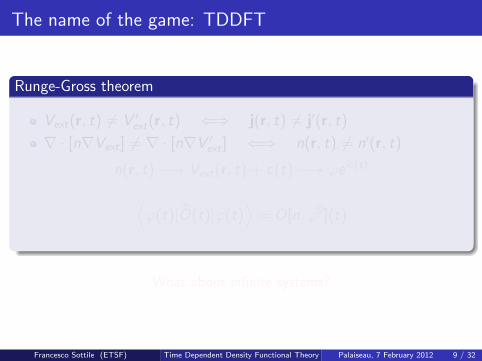
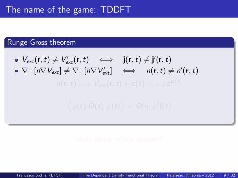
Runge-Gross theorem
Vext(r, t) 6= V ′ext(r, t) ⇐⇒ j(r, t) 6= j′(r, t)
∇ · [n∇Vext ] 6= ∇ · [n∇V ′ext ] ⇐⇒ n(r, t) 6= n′(r, t)
n(r, t) −→ Vext(r, t) + c(t) −→ ϕe ic(t)⟨ϕ(t)|O(t)|ϕ(t)
⟩= O[n, ϕ0](t)
What about infinite systems?
Francesco Sottile (ETSF) Time Dependent Density Functional Theory Palaiseau, 7 February 2012 9 / 32

The name of the game: TDDFT
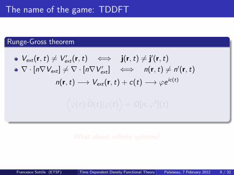
Runge-Gross theorem
Vext(r, t) 6= V ′ext(r, t) ⇐⇒ j(r, t) 6= j′(r, t)
∇ · [n∇Vext ] 6= ∇ · [n∇V ′ext ] ⇐⇒ n(r, t) 6= n′(r, t)
n(r, t) −→ Vext(r, t) + c(t) −→ ϕe ic(t)⟨ϕ(t)|O(t)|ϕ(t)
⟩= O[n, ϕ0](t)
What about infinite systems?
Francesco Sottile (ETSF) Time Dependent Density Functional Theory Palaiseau, 7 February 2012 9 / 32
The name of the game: TDDFT
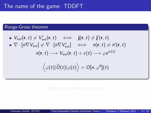
Runge-Gross theorem
Vext(r, t) 6= V ′ext(r, t) ⇐⇒ j(r, t) 6= j′(r, t)
∇ · [n∇Vext ] 6= ∇ · [n∇V ′ext ] ⇐⇒ n(r, t) 6= n′(r, t)
n(r, t) −→ Vext(r, t) + c(t) −→ ϕe ic(t)⟨ϕ(t)|O(t)|ϕ(t)
⟩= O[n, ϕ0](t)
What about infinite systems?
Francesco Sottile (ETSF) Time Dependent Density Functional Theory Palaiseau, 7 February 2012 9 / 32
The name of the game: TDDFT
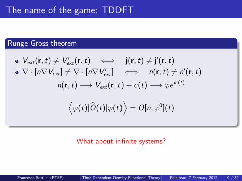
Runge-Gross theorem
Vext(r, t) 6= V ′ext(r, t) ⇐⇒ j(r, t) 6= j′(r, t)
∇ · [n∇Vext ] 6= ∇ · [n∇V ′ext ] ⇐⇒ n(r, t) 6= n′(r, t)
n(r, t) −→ Vext(r, t) + c(t) −→ ϕe ic(t)⟨ϕ(t)|O(t)|ϕ(t)
⟩= O[n, ϕ0](t)
What about infinite systems?
Francesco Sottile (ETSF) Time Dependent Density Functional Theory Palaiseau, 7 February 2012 9 / 32
The name of the game: TDDFT
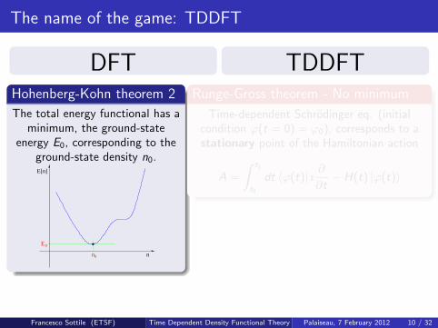
DFT TDDFTHohenberg-Kohn theorem 2
The total energy functional has aminimum, the ground-state
energy E0, corresponding to theground-state density n0.
n
E[n]
n0
0E
Runge-Gross theorem - No minimum
Time-dependent Schrodinger eq. (initialcondition ϕ(t = 0) = ϕ0), corresponds to astationary point of the Hamiltonian action
A =
∫ t1
t0
dt 〈ϕ(t)| ı ∂∂t− H(t) |ϕ(t)〉
Francesco Sottile (ETSF) Time Dependent Density Functional Theory Palaiseau, 7 February 2012 10 / 32
The name of the game: TDDFT
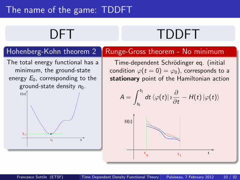
DFT TDDFTHohenberg-Kohn theorem 2
The total energy functional has aminimum, the ground-state
energy E0, corresponding to theground-state density n0.
n
E[n]
n0
0E
Runge-Gross theorem - No minimum
Time-dependent Schrodinger eq. (initialcondition ϕ(t = 0) = ϕ0), corresponds to astationary point of the Hamiltonian action
A =
∫ t1
t0
dt 〈ϕ(t)| ı ∂∂t− H(t) |ϕ(t)〉
tt 1t
0
H[t]
Francesco Sottile (ETSF) Time Dependent Density Functional Theory Palaiseau, 7 February 2012 10 / 32
The name of the game: TDDFT
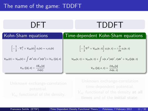
DFT TDDFTKohn-Sham equations
[−
1
2· ∇2
i + Vtot (r)
]φi (r) = εiφi (r)
Vtot (r) = Vext (r)+
∫dr′v(r, r′)n(r′)+Vxc ([n], r)
Vxc ([n], r) =δExc [n]
δn(r)
Time-dependent Kohn-Sham equations
[−
1
2∇2 + Vtot (r, t)
]φi (r, t) = i
∂
∂tφi (r, t)
Vtot (r, t) = Vext (r, t) +
∫v(r, r′)n(r′, t)dr′ + Vxc ([n]r, t)
Vxc ([n], r, t) =δAxc [n]
δn(r, t)
Unknown exchange-correlationpotential.
Vxc functional of the density.
Unknown exchange-correlationtime-dependent potential.
Vxc functional of the density at alltimes and of the initial state.
Francesco Sottile (ETSF) Time Dependent Density Functional Theory Palaiseau, 7 February 2012 11 / 32
The name of the game: TDDFT
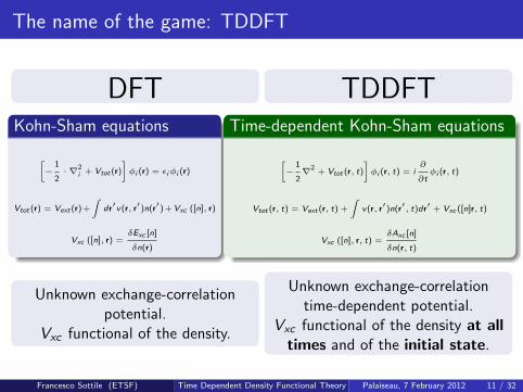
DFT TDDFTKohn-Sham equations
[−
1
2· ∇2
i + Vtot (r)
]φi (r) = εiφi (r)
Vtot (r) = Vext (r)+
∫dr′v(r, r′)n(r′)+Vxc ([n], r)
Vxc ([n], r) =δExc [n]
δn(r)
Time-dependent Kohn-Sham equations
[−
1
2∇2 + Vtot (r, t)
]φi (r, t) = i
∂
∂tφi (r, t)
Vtot (r, t) = Vext (r, t) +
∫v(r, r′)n(r′, t)dr′ + Vxc ([n]r, t)
Vxc ([n], r, t) =δAxc [n]
δn(r, t)
Unknown exchange-correlationpotential.
Vxc functional of the density.
Unknown exchange-correlationtime-dependent potential.
Vxc functional of the density at alltimes and of the initial state.
Francesco Sottile (ETSF) Time Dependent Density Functional Theory Palaiseau, 7 February 2012 11 / 32
The name of the game: TDDFT
Demonstrations, further readings, etc.
R. van LeeuwenInt.J.Mod.Phys. B15, 1969 (2001)
Vxc ([n], r, t) =δAxc [n]
δn(r, t)
δVxc ([n], r, t)
δn(r′, t ′)=
δ2Axc [n]
δn(r, t)δn(r′, t ′)
Causality-Symmetry dilemma
Francesco Sottile (ETSF) Time Dependent Density Functional Theory Palaiseau, 7 February 2012 12 / 32
The name of the game: TDDFT
DFT TDDFTHohenberg-Kohn theoremThe ground-state expectation value
of any physical observable of amany-electrons system is a uniquefunctional of the electron density
n(r)⟨ϕ0∣∣∣ O ∣∣∣ϕ0
⟩= O[n]
Kohn-Sham equations
[−1
2∇2
i + Vtot(r)
]φi (r) = εiφi (r)
Runge-Gross theoremThe expectation value of any physical
time-dependent observable of a many-electronssystem is a unique functional of the
time-dependent electron density n(r) and of theinitial state ϕ0 = ϕ(t = 0)⟨ϕ(t)|O(t)|ϕ(t)
⟩= O[n, ϕ0](t)
Kohn-Sham equations
[−1
2∇2 + Vtot(r, t)
]φi (r, t) = i
∂
∂tφi (r, t)
Francesco Sottile (ETSF) Time Dependent Density Functional Theory Palaiseau, 7 February 2012 13 / 32
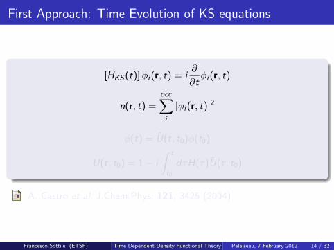
First Approach: Time Evolution of KS equations
[HKS(t)]φi (r, t) = i∂
∂tφi (r, t)
n(r, t) =occ∑i
|φi (r, t)|2
φ(t) = U(t, t0)φ(t0)
U(t, t0) = 1− i
∫ t
t0
dτH(τ)U(τ, t0)
A. Castro et al. J.Chem.Phys. 121, 3425 (2004)
Francesco Sottile (ETSF) Time Dependent Density Functional Theory Palaiseau, 7 February 2012 14 / 32
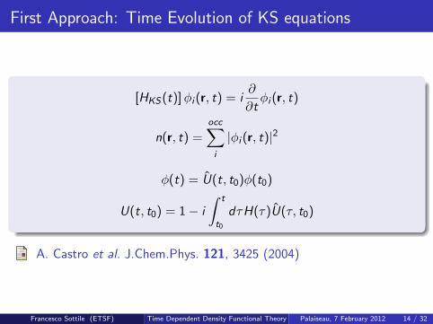
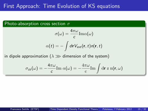
First Approach: Time Evolution of KS equations
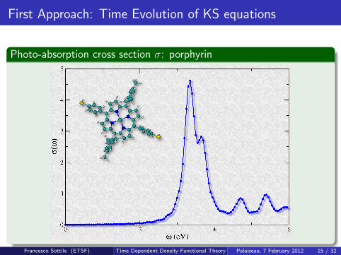
Photo-absorption cross section σ
σ(ω) =4πω
cImα(ω)
α(t) = −∫
drVext(r, t)n(r, t)
in dipole approximation (λ≫ dimension of the system)
σzz(ω) = −4πω
cIm α(ω) = −4πω
cIm
∫dr z n(r, ω)
Francesco Sottile (ETSF) Time Dependent Density Functional Theory Palaiseau, 7 February 2012 15 / 32
First Approach: Time Evolution of KS equations
Photo-absorption cross section σ: porphyrin
Francesco Sottile (ETSF) Time Dependent Density Functional Theory Palaiseau, 7 February 2012 15 / 32
First Approach: Time Evolution of KS equations
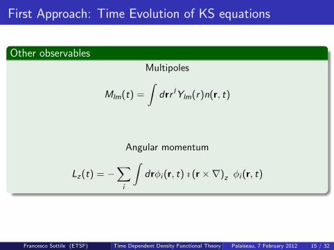
Other observables
Multipoles
Mlm(t) =
∫drr lYlm(r)n(r, t)
Angular momentum
Lz(t) = −∑i
∫drφi (r, t) ı (r ×∇)z φi (r, t)
Francesco Sottile (ETSF) Time Dependent Density Functional Theory Palaiseau, 7 February 2012 15 / 32
First Approach: Time Evolution of KS equations
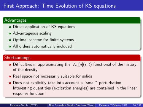
Advantages
Direct application of KS equations
Advantageous scaling
Optimal scheme for finite systems
All orders automatically included
Shortcomings
Difficulties in approximating the Vxc [n](r, t) functional of the historyof the density
Real space not necessarily suitable for solids
Does not explicitly take into account a “small” perturbation.Interesting quantities (excitation energies) are contained in the linearresponse function!
Francesco Sottile (ETSF) Time Dependent Density Functional Theory Palaiseau, 7 February 2012 16 / 32
Outline
1 Introduction: why TD-DFT ?
2 (Just) A bit of Formalism - The Boring PartTDDFT: the FoundationLinear Response Formalism
3 TDDFT in practice:The ALDA: Achievements and ShortcomingsThe Quest for the Holy FunctionalNew Frontiers
4 Perspectives and Resources
Francesco Sottile (ETSF) Time Dependent Density Functional Theory Palaiseau, 7 February 2012 17 / 32
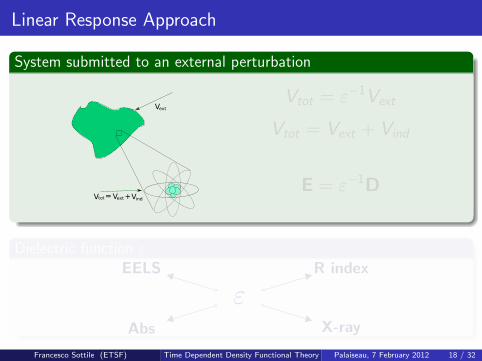
Linear Response Approach
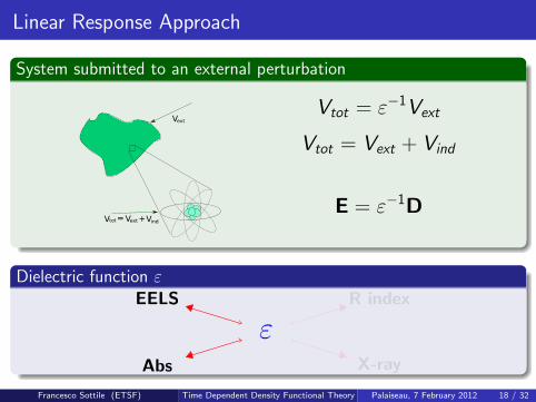
System submitted to an external perturbation
Vtot = ε−1Vext
Vtot = Vext + Vind
E = ε−1D
Dielectric function ε
Abs
EELS
εX-ray
R index
Francesco Sottile (ETSF) Time Dependent Density Functional Theory Palaiseau, 7 February 2012 18 / 32
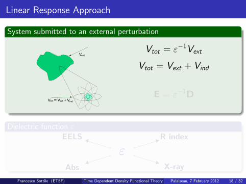
Linear Response Approach
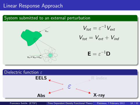
System submitted to an external perturbation
Vtot = ε−1Vext
Vtot = Vext + Vind
E = ε−1D
Dielectric function ε
Abs
EELS
εX-ray
R index
Francesco Sottile (ETSF) Time Dependent Density Functional Theory Palaiseau, 7 February 2012 18 / 32

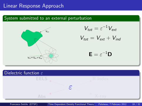
Linear Response Approach
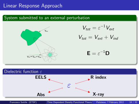
System submitted to an external perturbation
Vtot = ε−1Vext
Vtot = Vext + Vind
E = ε−1D
Dielectric function ε
Abs
EELS
εX-ray
R index
Francesco Sottile (ETSF) Time Dependent Density Functional Theory Palaiseau, 7 February 2012 18 / 32
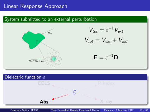
Linear Response Approach
System submitted to an external perturbation
Vtot = ε−1Vext
Vtot = Vext + Vind
E = ε−1D
Dielectric function ε
Abs
EELS
εX-ray
R index
Francesco Sottile (ETSF) Time Dependent Density Functional Theory Palaiseau, 7 February 2012 18 / 32
Linear Response Approach
System submitted to an external perturbation
Vtot = ε−1Vext
Vtot = Vext + Vind
E = ε−1D
Dielectric function ε
Abs
EELS
εX-ray
R index
Francesco Sottile (ETSF) Time Dependent Density Functional Theory Palaiseau, 7 February 2012 18 / 32
Linear Response Approach
System submitted to an external perturbation
Vtot = ε−1Vext
Vtot = Vext + Vind
E = ε−1D
Dielectric function ε
Abs
EELS
εX-ray
R index
Francesco Sottile (ETSF) Time Dependent Density Functional Theory Palaiseau, 7 February 2012 18 / 32
Linear Response Approach
System submitted to an external perturbation
Vtot = ε−1Vext
Vtot = Vext + Vind
E = ε−1D
Dielectric function ε
Abs
EELS
εX-ray
R index
Francesco Sottile (ETSF) Time Dependent Density Functional Theory Palaiseau, 7 February 2012 18 / 32
Linear Response Approach
System submitted to an external perturbation
Vtot = ε−1Vext
Vtot = Vext + Vind
E = ε−1D
Dielectric function ε
Abs
EELS
εX-ray
R index
Francesco Sottile (ETSF) Time Dependent Density Functional Theory Palaiseau, 7 February 2012 18 / 32
Linear Response Approach
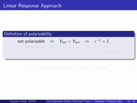
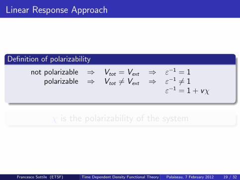
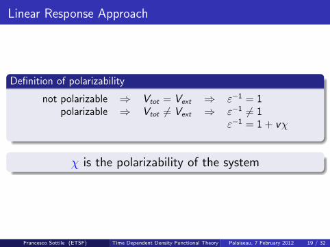
Definition of polarizability
not polarizable ⇒ Vtot = Vext ⇒ ε−1 = 1polarizable ⇒ Vtot 6= Vext ⇒ ε−1 6= 1
ε−1 = 1 + vχ
χ is the polarizability of the system
Francesco Sottile (ETSF) Time Dependent Density Functional Theory Palaiseau, 7 February 2012 19 / 32

Linear Response Approach
Definition of polarizability
not polarizable ⇒ Vtot = Vext ⇒ ε−1 = 1polarizable ⇒ Vtot 6= Vext ⇒ ε−1 6= 1
ε−1 = 1 + vχ
χ is the polarizability of the system
Francesco Sottile (ETSF) Time Dependent Density Functional Theory Palaiseau, 7 February 2012 19 / 32
Linear Response Approach
Definition of polarizability
not polarizable ⇒ Vtot = Vext ⇒ ε−1 = 1polarizable ⇒ Vtot 6= Vext ⇒ ε−1 6= 1
ε−1 = 1 + vχ
χ is the polarizability of the system
Francesco Sottile (ETSF) Time Dependent Density Functional Theory Palaiseau, 7 February 2012 19 / 32
Linear Response Approach
Definition of polarizability
not polarizable ⇒ Vtot = Vext ⇒ ε−1 = 1polarizable ⇒ Vtot 6= Vext ⇒ ε−1 6= 1
ε−1 = 1 + vχ
χ is the polarizability of the system
Francesco Sottile (ETSF) Time Dependent Density Functional Theory Palaiseau, 7 February 2012 19 / 32
Linear Response Approach
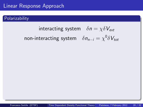
Polarizability
interacting system δn = χδVext
non-interacting system δnn−i = χ0δVtot
Francesco Sottile (ETSF) Time Dependent Density Functional Theory Palaiseau, 7 February 2012 20 / 32

Linear Response Approach
Polarizability
interacting system δn = χδVext
non-interacting system δnn−i = χ0δVtot
Single-particle polarizability
χ0 =∑ij
φi (r)φ∗j (r)φ∗i (r′)φj(r′)
ω − (εi − εj)
hartree, hartree-fock, dft, etc.
G.D. Mahan Many Particle Physics (Plenum, New York, 1990)
Francesco Sottile (ETSF) Time Dependent Density Functional Theory Palaiseau, 7 February 2012 20 / 32

Linear Response Approach
Polarizability
interacting system δn = χδVext
non-interacting system δnn−i = χ0δVtot
χ0 =∑ij
φi (r)φ∗j (r)φ∗i (r′)φj(r′)
ω − (εi − εj)
i
unoccupied states
occupied states
j
Francesco Sottile (ETSF) Time Dependent Density Functional Theory Palaiseau, 7 February 2012 20 / 32
Linear Response Approach
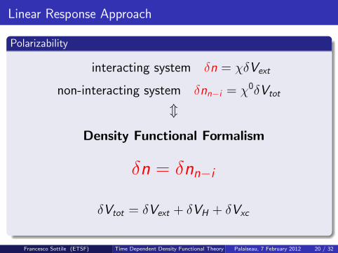
Polarizability
interacting system δn = χδVext
non-interacting system δnn−i = χ0δVtot
m
Density Functional Formalism
δn = δnn−i
δVtot = δVext + δVH + δVxc
Francesco Sottile (ETSF) Time Dependent Density Functional Theory Palaiseau, 7 February 2012 20 / 32

Linear Response Approach
Polarizability
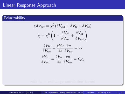
χδVext = χ0 (δVext + δVH + δVxc)
χ = χ0
(1 +
δVH
δVext+δVxc
δVext
)δVH
δVext=δVH
δn
δn
δVext= vχ
δVxc
δVext=δVxc
δn
δn
δVext= fxcχ
with fxc = exchange-correlation kernel
Francesco Sottile (ETSF) Time Dependent Density Functional Theory Palaiseau, 7 February 2012 21 / 32
Linear Response Approach
Polarizability
χδVext = χ0 (δVext + δVH + δVxc)
χ = χ0
(1 +
δVH
δVext+δVxc
δVext
)δVH
δVext=δVH
δn
δn
δVext= vχ
δVxc
δVext=δVxc
δn
δn
δVext= fxcχ
with fxc = exchange-correlation kernel
Francesco Sottile (ETSF) Time Dependent Density Functional Theory Palaiseau, 7 February 2012 21 / 32

Linear Response Approach
Polarizability
χδVext = χ0 (δVext + δVH + δVxc)
χ = χ0
(1 +
δVH
δVext+δVxc
δVext
)δVH
δVext=δVH
δn
δn
δVext= vχ
δVxc
δVext=δVxc
δn
δn
δVext= fxcχ
χ = χ0 + χ0 (v + fxc)χwith fxc = exchange-correlation kernel
Francesco Sottile (ETSF) Time Dependent Density Functional Theory Palaiseau, 7 February 2012 21 / 32
Linear Response Approach
Polarizability
χδVext = χ0 (δVext + δVH + δVxc)
χ = χ0
(1 +
δVH
δVext+δVxc
δVext
)δVH
δVext=δVH
δn
δn
δVext= vχ
δVxc
δVext=δVxc
δn
δn
δVext= fxcχ
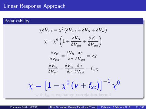
χ =[1− χ0 (v + fxc)
]−1χ0
with fxc = exchange-correlation kernel
Francesco Sottile (ETSF) Time Dependent Density Functional Theory Palaiseau, 7 February 2012 21 / 32
Linear Response Approach
Polarizability
χδVext = χ0 (δVext + δVH + δVxc)
χ = χ0
(1 +
δVH
δVext+δVxc
δVext
)δVH
δVext=δVH
δn
δn
δVext= vχ
δVxc
δVext=δVxc
δn
δn
δVext= fxcχ
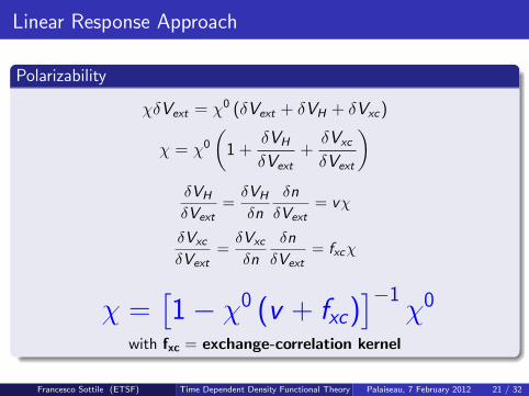
χ =[1− χ0 (v + fxc)
]−1χ0
with fxc = exchange-correlation kernel
Francesco Sottile (ETSF) Time Dependent Density Functional Theory Palaiseau, 7 February 2012 21 / 32
Linear Response Approach
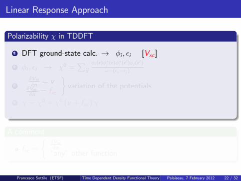
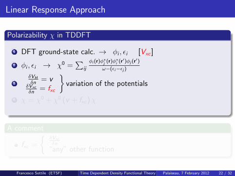
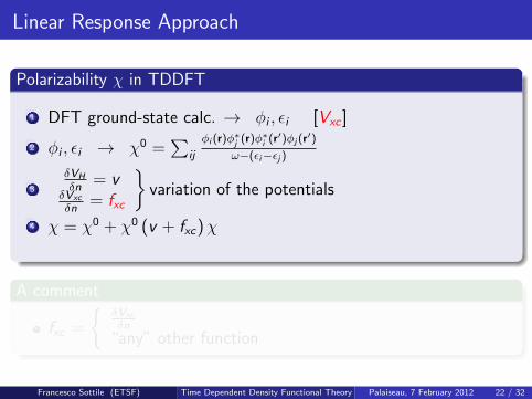
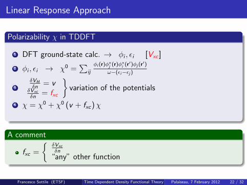
Polarizability χ in TDDFT
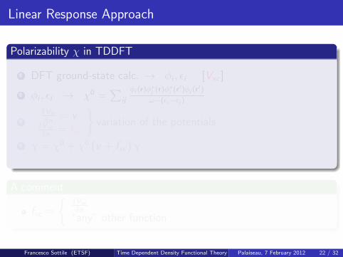
1 DFT ground-state calc. → φi , εi [Vxc ]
2 φi , εi → χ0 =∑
ij
φi (r)φ∗j (r)φ
∗i (r′)φj (r
′)
ω−(εi−εj )
3
δVH
δn= v
δVxc
δn= fxc
variation of the potentials
4 χ = χ0 + χ0 (v + fxc)χ
A comment
fxc =
δVxc
δn“any” other function
Francesco Sottile (ETSF) Time Dependent Density Functional Theory Palaiseau, 7 February 2012 22 / 32
Linear Response Approach
Polarizability χ in TDDFT
1 DFT ground-state calc. → φi , εi [Vxc ]
2 φi , εi → χ0 =∑
ij
φi (r)φ∗j (r)φ
∗i (r′)φj (r
′)
ω−(εi−εj )
3
δVH
δn= v
δVxc
δn= fxc
variation of the potentials
4 χ = χ0 + χ0 (v + fxc)χ
A comment
fxc =
δVxc
δn“any” other function
Francesco Sottile (ETSF) Time Dependent Density Functional Theory Palaiseau, 7 February 2012 22 / 32
Finite systems
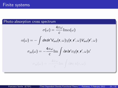
Photo-absorption cross spectrum
σ(ω) =4πω
cImα(ω)
α(ω) = −∫
drdr′Vext(r, ω)χ(r, r′, ω)Vext(r′, ω)
σzz(ω) = −4πω
cIm
∫drdr′zχ(r, r′, ω)z′
σzz(ω) = −4πω
cIm
∫drz n(r, ω)
Francesco Sottile (ETSF) Time Dependent Density Functional Theory Palaiseau, 7 February 2012 23 / 32
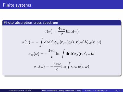
Finite systems
Photo-absorption cross spectrum
σ(ω) =4πω
cImα(ω)
α(ω) = −∫
drdr′Vext(r, ω)χ(r, r′, ω)Vext(r′, ω)
σzz(ω) = −4πω
cIm
∫drdr′zχ(r, r′, ω)z′
σzz(ω) = −4πω
cIm
∫drz n(r, ω)
Francesco Sottile (ETSF) Time Dependent Density Functional Theory Palaiseau, 7 February 2012 23 / 32

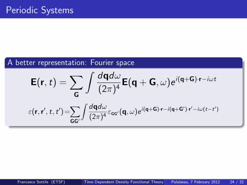
Periodic Systems
A better representation: Fourier space
E(r, t) =∑
G
∫dqdω
(2π)4E(q + G, ω)e i(q+G)·r−iωt
ε(r, r′, t, t ′)=∑GG′
∫dqdω
(2π)4εGG′(q, ω)e i(q+G)·r−i(q+G′)·r′−iω(t−t′)
Francesco Sottile (ETSF) Time Dependent Density Functional Theory Palaiseau, 7 February 2012 24 / 32
Periodic Systems
A better representation: Fourier space
E(r, t) =∑
G
∫dqdω
(2π)4E(q + G, ω)e i(q+G)·r−iωt
ε(r, r′, t, t ′)=∑GG′
∫dqdω
(2π)4εGG′(q, ω)e i(q+G)·r−i(q+G′)·r′−iω(t−t′)
Francesco Sottile (ETSF) Time Dependent Density Functional Theory Palaiseau, 7 February 2012 24 / 32
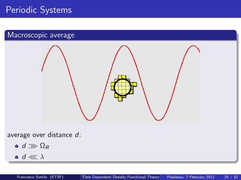
Periodic Systems
Macroscopic average
average over distance d :
d ≫ ΩR
d ≪ λ
Francesco Sottile (ETSF) Time Dependent Density Functional Theory Palaiseau, 7 February 2012 25 / 32

Periodic Systems
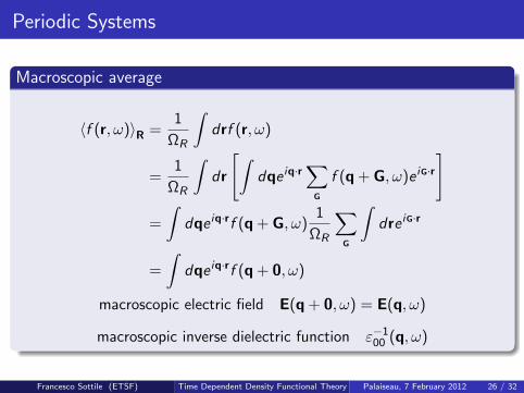
Macroscopic average
〈f (r, ω)〉R =1
ΩR
∫drf (r, ω)
=1
ΩR
∫dr
[∫dqe iq·r
∑G
f (q + G, ω)e iG·r
]
=
∫dqe iq·rf (q + G, ω)
1
ΩR
∑G
∫dre iG·r
=
∫dqe iq·rf (q + 0, ω)
macroscopic electric field E(q + 0, ω) = E(q, ω)
macroscopic inverse dielectric function ε−100 (q, ω)
Francesco Sottile (ETSF) Time Dependent Density Functional Theory Palaiseau, 7 February 2012 26 / 32

Periodic Systems
Macroscopic average
〈f (r, ω)〉R =1
ΩR
∫drf (r, ω)
=1
ΩR
∫dr
[∫dqe iq·r
∑G
f (q + G, ω)e iG·r
]
=
∫dqe iq·rf (q + G, ω)
1
ΩR
∑G
∫dre iG·r
=
∫dqe iq·rf (q + 0, ω)
macroscopic electric field E(q + 0, ω) = E(q, ω)
macroscopic inverse dielectric function ε−100 (q, ω)
Francesco Sottile (ETSF) Time Dependent Density Functional Theory Palaiseau, 7 February 2012 26 / 32
Absorption coefficient
General solution of Maxwell’s equation
in vacuum E(x , t) = E0eiω(x/c−t)
in a medium E(x , t) = E0eiω(Nx/c−t)
Francesco Sottile (ETSF) Time Dependent Density Functional Theory Palaiseau, 7 February 2012 27 / 32

Absorption coefficient
General solution of Maxwell’s equation
in vacuum E(x , t) = E0eiω(x/c−t)
in a medium E(x , t) = E0eiω(Nx/c−t)
Francesco Sottile (ETSF) Time Dependent Density Functional Theory Palaiseau, 7 February 2012 27 / 32

Absorption coefficient
General solution of Maxwell’s equation
in vacuum E(x , t) = E0eiω(x/c−t)
in a medium E(x , t) = E0eiω(Nx/c−t)
complex (macroscopic) refractive index N
N =√εM = ν + iκ ; D = εME
absorption coefficient α (inverse distance∣∣ |E(x)|2|E0|2 = 1
e )
α =ωImεMνc
Francesco Sottile (ETSF) Time Dependent Density Functional Theory Palaiseau, 7 February 2012 27 / 32
Absorption coefficient
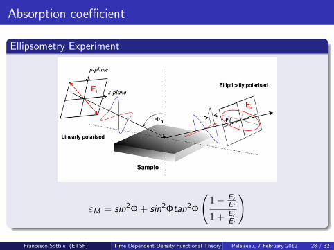
Ellipsometry Experiment
εM = sin2Φ + sin2Φtan2Φ
(1− Er
Ei
1 + ErEi
)
Francesco Sottile (ETSF) Time Dependent Density Functional Theory Palaiseau, 7 February 2012 28 / 32
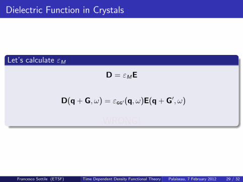
Dielectric Function in Crystals
Let’s calculate εM
D = εME
WRONG!
Francesco Sottile (ETSF) Time Dependent Density Functional Theory Palaiseau, 7 February 2012 29 / 32
Dielectric Function in Crystals
Let’s calculate εM
D = εME
D(q + G, ω) = εGG′(q, ω)E(q + G′, ω)
WRONG!
Francesco Sottile (ETSF) Time Dependent Density Functional Theory Palaiseau, 7 February 2012 29 / 32
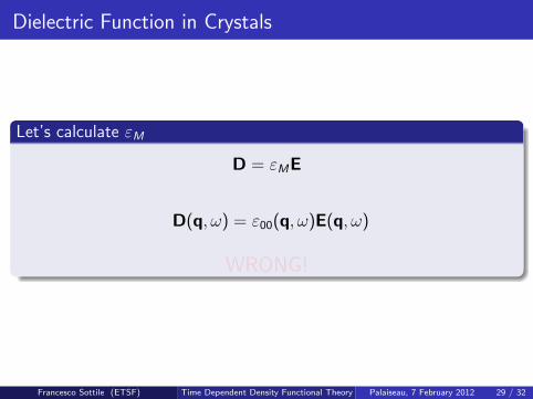
Dielectric Function in Crystals
Let’s calculate εM
D = εME
D(q, ω) = ε00(q, ω)E(q, ω)
WRONG!
Francesco Sottile (ETSF) Time Dependent Density Functional Theory Palaiseau, 7 February 2012 29 / 32
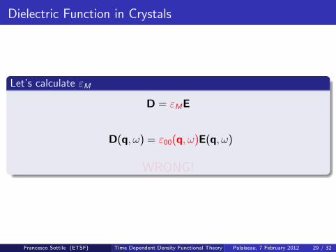
Dielectric Function in Crystals
Let’s calculate εM
D = εME
D(q, ω) = ε00(q, ω)E(q, ω)
WRONG!
Francesco Sottile (ETSF) Time Dependent Density Functional Theory Palaiseau, 7 February 2012 29 / 32

Dielectric Function in Crystals
Let’s calculate εM
D = εME
D(q, ω) = ε00(q, ω)E(q, ω)
WRONG!
Francesco Sottile (ETSF) Time Dependent Density Functional Theory Palaiseau, 7 February 2012 29 / 32
Dielectric Function in Crystals
Let’s calculate εM
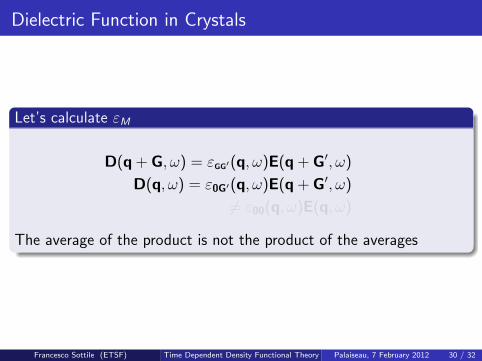
D(q + G, ω) = εGG′(q, ω)E(q + G′, ω)
D(q, ω) = ε0G′(q, ω)E(q + G′, ω)
6= ε00(q, ω)E(q, ω)
The average of the product is not the product of the averages
Francesco Sottile (ETSF) Time Dependent Density Functional Theory Palaiseau, 7 February 2012 30 / 32
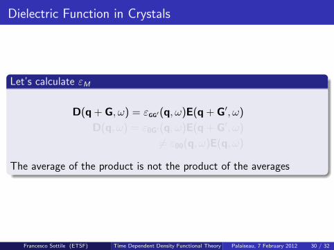
Dielectric Function in Crystals
Let’s calculate εM
D = εME
E(q + G, ω) = ε−1GG′(q, ω)D(q + G′, ω)
E(q + G, ω) = ε−1G0(q, ω)D(q, ω)
E(q, ω) = ε−100 (q, ω)D(q, ω)
εM =1
ε−100
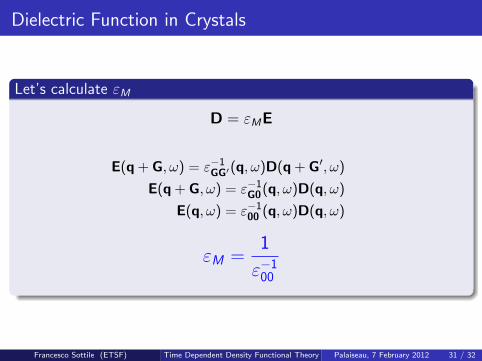
Francesco Sottile (ETSF) Time Dependent Density Functional Theory Palaiseau, 7 February 2012 31 / 32
Dielectric Function in Crystals
Let’s calculate εM
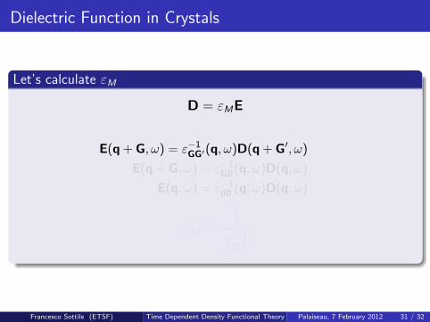
D = εME
E(q + G, ω) = ε−1GG′(q, ω)D(q + G′, ω)
E(q + G, ω) = ε−1G0(q, ω)D(q, ω)
E(q, ω) = ε−100 (q, ω)D(q, ω)
εM =1
ε−100
Francesco Sottile (ETSF) Time Dependent Density Functional Theory Palaiseau, 7 February 2012 31 / 32
Dielectric Function in Crystals
Let’s calculate εM
D = εME
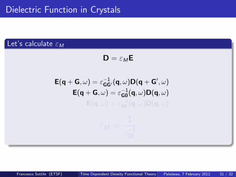
E(q + G, ω) = ε−1GG′(q, ω)D(q + G′, ω)
E(q + G, ω) = ε−1G0(q, ω)D(q, ω)
E(q, ω) = ε−100 (q, ω)D(q, ω)
εM =1
ε−100
Francesco Sottile (ETSF) Time Dependent Density Functional Theory Palaiseau, 7 February 2012 31 / 32
Dielectric Function in Crystals
Let’s calculate εM
D = εME
E(q + G, ω) = ε−1GG′(q, ω)D(q + G′, ω)
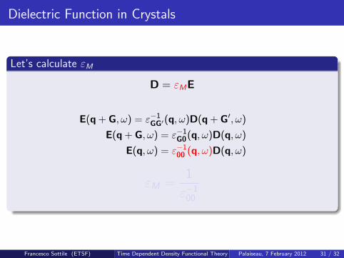
E(q + G, ω) = ε−1G0(q, ω)D(q, ω)
E(q, ω) = ε−100 (q, ω)D(q, ω)
εM =1
ε−100
Francesco Sottile (ETSF) Time Dependent Density Functional Theory Palaiseau, 7 February 2012 31 / 32
Dielectric Function in Crystals
Let’s calculate εM
D = εME
E(q + G, ω) = ε−1GG′(q, ω)D(q + G′, ω)
E(q + G, ω) = ε−1G0(q, ω)D(q, ω)
E(q, ω) = ε−100 (q, ω)D(q, ω)
εM =1
ε−100
Francesco Sottile (ETSF) Time Dependent Density Functional Theory Palaiseau, 7 February 2012 31 / 32
Dielectric Function in Crystals
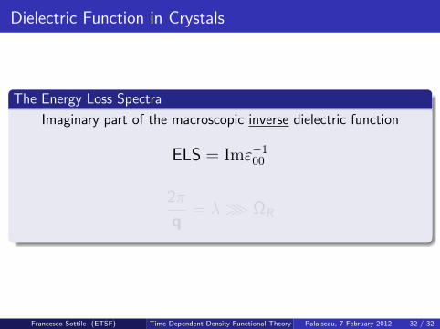
The Energy Loss Spectra
Imaginary part of the macroscopic inverse dielectric function
ELS = Imε−100
2π
q= λ≫ ΩR
Francesco Sottile (ETSF) Time Dependent Density Functional Theory Palaiseau, 7 February 2012 32 / 32
Dielectric Function in Crystals
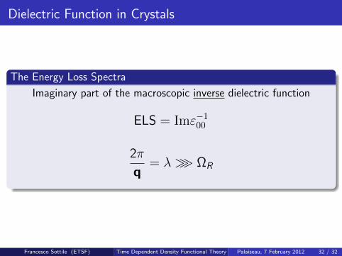
The Energy Loss Spectra
Imaginary part of the macroscopic inverse dielectric function
ELS = Imε−100
2π
q= λ≫ ΩR
Francesco Sottile (ETSF) Time Dependent Density Functional Theory Palaiseau, 7 February 2012 32 / 32
Dielectric Function in Crystals
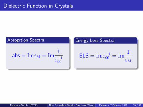
Absoprtion Spectra
abs = ImεM = Im1
ε−100
Energy Loss Spectra
ELS = Imε−100 = Im
1
εM
Francesco Sottile (ETSF) Time Dependent Density Functional Theory Palaiseau, 7 February 2012 33 / 32
Dielectric Function in Crystals
Question
ε00 is not the macroscopic dielectric functionWhat is it then ?
ε00 is the macroscopic dielectric function ...without local fields.
Francesco Sottile (ETSF) Time Dependent Density Functional Theory Palaiseau, 7 February 2012 34 / 32
Dielectric Function in Crystals
Question
ε00 is not the macroscopic dielectric functionWhat is it then ?
ε00 is the macroscopic dielectric function ...without local fields.
Francesco Sottile (ETSF) Time Dependent Density Functional Theory Palaiseau, 7 February 2012 34 / 32

Dielectric Function in Crystals
Question
ε00 is not the macroscopic dielectric functionWhat is it then ?
ε00 is the macroscopic dielectric function ...without local fields.
Francesco Sottile (ETSF) Time Dependent Density Functional Theory Palaiseau, 7 February 2012 34 / 32
Solids
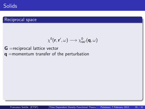
Reciprocal space
χ0(r, r′, ω) −→ χ0GG′(q, ω)
G =reciprocal lattice vectorq =momentum transfer of the perturbation
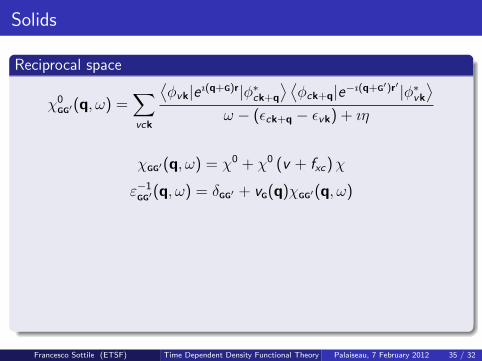
S.L.Adler, Phys.Rev 126, 413 (1962); N.Wiser Phys.Rev 129, 62 (1963)
Francesco Sottile (ETSF) Time Dependent Density Functional Theory Palaiseau, 7 February 2012 35 / 32
Solids
Reciprocal space
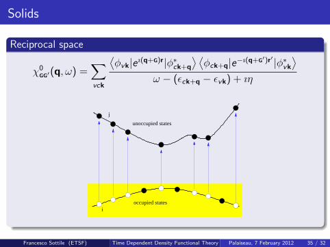
χ0GG′(q, ω) =
∑vck
⟨φvk|eı(q+G)r|φ∗ck+q
⟩ ⟨φck+q|e−ı(q+G′)r′|φ∗vk
⟩ω − (εck+q − εvk) + ıη
i
unoccupied states
occupied states
j
S.L.Adler, Phys.Rev 126, 413 (1962); N.Wiser Phys.Rev 129, 62 (1963)
Francesco Sottile (ETSF) Time Dependent Density Functional Theory Palaiseau, 7 February 2012 35 / 32
Solids
Reciprocal space
χ0GG′(q, ω) =
∑vck
⟨φvk|eı(q+G)r|φ∗ck+q
⟩ ⟨φck+q|e−ı(q+G′)r′|φ∗vk
⟩ω − (εck+q − εvk) + ıη
χGG′(q, ω) = χ0 + χ0 (v + fxc)χ
ε−1GG′(q, ω) = δGG′ + vG(q)χGG′(q, ω)
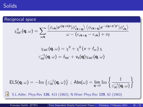
ELS(q, ω) = −Imε−100 (q, ω)
; Abs(ω) = lim
q→0Im
1
ε−100 (q, ω)
S.L.Adler, Phys.Rev 126, 413 (1962); N.Wiser Phys.Rev 129, 62 (1963)
Francesco Sottile (ETSF) Time Dependent Density Functional Theory Palaiseau, 7 February 2012 35 / 32

Solids
Reciprocal space
χ0GG′(q, ω) =
∑vck
⟨φvk|eı(q+G)r|φ∗ck+q
⟩ ⟨φck+q|e−ı(q+G′)r′|φ∗vk
⟩ω − (εck+q − εvk) + ıη
χGG′(q, ω) = χ0 + χ0 (v + fxc)χ
ε−1GG′(q, ω) = δGG′ + vG(q)χGG′(q, ω)
ELS(ω) =− limq→0
Imε−100 (q, ω)
; Abs(ω) = lim
q→0Im
1
ε−100 (q, ω)
S.L.Adler, Phys.Rev 126, 413 (1962); N.Wiser Phys.Rev 129, 62 (1963)
Francesco Sottile (ETSF) Time Dependent Density Functional Theory Palaiseau, 7 February 2012 35 / 32
Solids
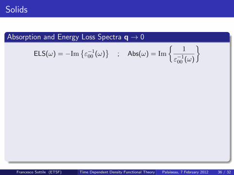
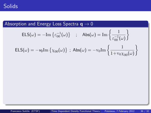
Absorption and Energy Loss Spectra q→ 0
ELS(ω) = −Imε−100 (ω)
; Abs(ω) = Im
1
ε−100 (ω)
ELS(ω) = −v0 Imχ00(ω)
; Abs(ω) = −v0 Im
χ00(ω)
χ = χ0 + χ0 (v + fxc)χ
χ = χ0 + χ0 (v + fxc) χ
vG =
vG ∀G 6= 00 G = 0
Exercise
Im
1
ε−100
= −v0Im
χ00
Francesco Sottile (ETSF) Time Dependent Density Functional Theory Palaiseau, 7 February 2012 36 / 32
Solids
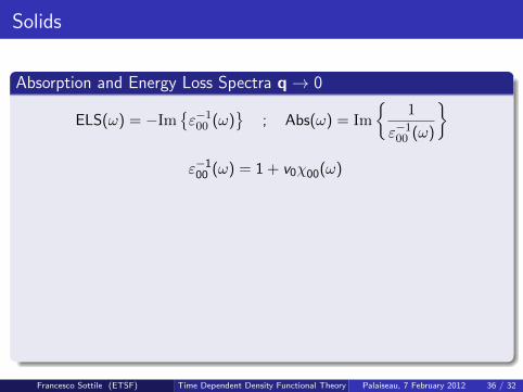
Absorption and Energy Loss Spectra q→ 0
ELS(ω) = −Imε−100 (ω)
; Abs(ω) = Im
1
ε−100 (ω)
ε−100 (ω) = 1 + v0χ00(ω)
ELS(ω) = −v0 Imχ00(ω)
; Abs(ω) = −v0 Im
χ00(ω)
χ = χ0 + χ0 (v + fxc)χ
χ = χ0 + χ0 (v + fxc) χ
vG =
vG ∀G 6= 00 G = 0
Exercise
Im
1
ε−100
= −v0Im
χ00
Francesco Sottile (ETSF) Time Dependent Density Functional Theory Palaiseau, 7 February 2012 36 / 32
Solids
Absorption and Energy Loss Spectra q→ 0
ELS(ω) = −Imε−100 (ω)
; Abs(ω) = Im
1
ε−100 (ω)
ELS(ω) = −v0Imχ00(ω)
; Abs(ω) = −v0Im
1
1+v0χ00(ω)
ELS(ω) = −v0 Im
χ00(ω)
; Abs(ω) = −v0 Im
χ00(ω)
χ = χ0 + χ0 (v + fxc)χ
χ = χ0 + χ0 (v + fxc) χ
vG =
vG ∀G 6= 00 G = 0
Exercise
Im
1
ε−100
= −v0Im
χ00
Francesco Sottile (ETSF) Time Dependent Density Functional Theory Palaiseau, 7 February 2012 36 / 32

Solids
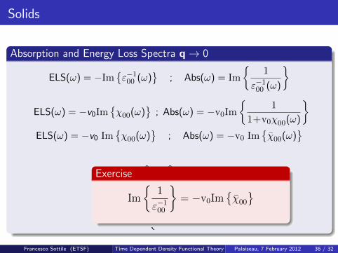
Absorption and Energy Loss Spectra q→ 0
ELS(ω) = −Imε−100 (ω)
; Abs(ω) = Im
1
ε−100 (ω)
ELS(ω) = −v0Imχ00(ω)
; Abs(ω) = −v0Im
1
1+v0χ00(ω)
ELS(ω) = −v0 Im
χ00(ω)
; Abs(ω) = −v0 Im
χ00(ω)
χ = χ0 + χ0 (v + fxc)χ
χ = χ0 + χ0 (v + fxc) χ
vG =
vG ∀G 6= 00 G = 0
Exercise
Im
1
ε−100
= −v0Im
χ00
Francesco Sottile (ETSF) Time Dependent Density Functional Theory Palaiseau, 7 February 2012 36 / 32
Solids
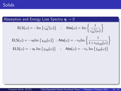
Absorption and Energy Loss Spectra q→ 0
ELS(ω) = −Imε−100 (ω)
; Abs(ω) = Im
1
ε−100 (ω)
ELS(ω) = −v0Imχ00(ω)
; Abs(ω) = −v0Im
1
1+v0χ00(ω)
ELS(ω) = −v0 Im
χ00(ω)
; Abs(ω) = −v0 Im
χ00(ω)
χ = χ0 + χ0 (v + fxc)χ
χ = χ0 + χ0 (v + fxc) χ
vG =
vG ∀G 6= 00 G = 0
Exercise
Im
1
ε−100
= −v0Im
χ00
Francesco Sottile (ETSF) Time Dependent Density Functional Theory Palaiseau, 7 February 2012 36 / 32

Solids
Abs and ELS (q→ 0) differs only by v0
ELS(ω) = −Imε−100 (ω)
; Abs(ω) = Im
1
ε−100 (ω)
ELS(ω) = −v0 Im
χ00(ω)
; Abs(ω) = −v0 Im
χ00(ω)
χ = χ0 + χ0 (v + fxc)χ
χ = χ0 + χ0 (v + fxc) χ
vG =
vG ∀G 6= 00 G = 0
microscopic components
Francesco Sottile (ETSF) Time Dependent Density Functional Theory Palaiseau, 7 February 2012 37 / 32
Solids
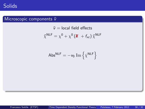
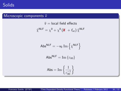
Microscopic components v
v = local field effects
χNLF = χ0 + χ0 (vX + fxc) χNLF
AbsNLF = −v0 ImχNLF
AbsNLF = Im ε00
Abs = Im
1
ε−100
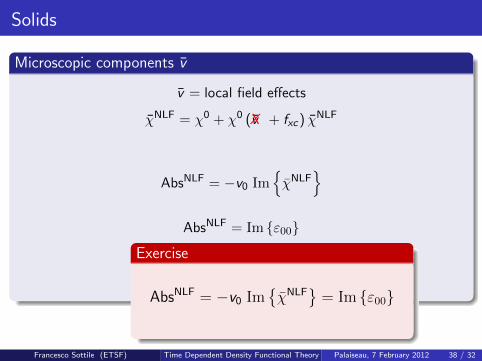
Exercise
AbsNLF = −v0 ImχNLF
= Im ε00
Francesco Sottile (ETSF) Time Dependent Density Functional Theory Palaiseau, 7 February 2012 38 / 32
Solids
Microscopic components v
v = local field effects
χNLF = χ0 + χ0 (vX + fxc) χNLF
AbsNLF = −v0 ImχNLF
AbsNLF = Im ε00
Abs = Im
1
ε−100
Exercise
AbsNLF = −v0 ImχNLF
= Im ε00
Francesco Sottile (ETSF) Time Dependent Density Functional Theory Palaiseau, 7 February 2012 38 / 32

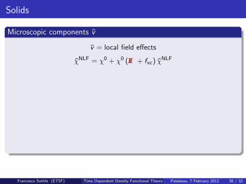
Solids
Microscopic components v
v = local field effects
χNLF = χ0 + χ0 (vX + fxc) χNLF
AbsNLF = −v0 ImχNLF
AbsNLF = Im ε00
Abs = Im
1
ε−100
Exercise
AbsNLF = −v0 ImχNLF
= Im ε00
Francesco Sottile (ETSF) Time Dependent Density Functional Theory Palaiseau, 7 February 2012 38 / 32
Solids
Microscopic components v
v = local field effects
χNLF = χ0 + χ0 (vX + fxc) χNLF
AbsNLF = −v0 ImχNLF
AbsNLF = Im ε00
Abs = Im
1
ε−100
Exercise
AbsNLF = −v0 ImχNLF
= Im ε00
Francesco Sottile (ETSF) Time Dependent Density Functional Theory Palaiseau, 7 February 2012 38 / 32
Solids
Microscopic components v
v = local field effects
χNLF = χ0 + χ0 (vX + fxc) χNLF
AbsNLF = −v0 ImχNLF
AbsNLF = Im ε00
Abs = Im
1
ε−100
Exercise
AbsNLF = −v0 ImχNLF
= Im ε00
Francesco Sottile (ETSF) Time Dependent Density Functional Theory Palaiseau, 7 February 2012 38 / 32
Outline
1 Introduction: why TD-DFT ?
2 (Just) A bit of Formalism - The Boring PartTDDFT: the FoundationLinear Response Formalism
3 TDDFT in practice:The ALDA: Achievements and ShortcomingsThe Quest for the Holy FunctionalNew Frontiers
4 Perspectives and Resources
Francesco Sottile (ETSF) Time Dependent Density Functional Theory Palaiseau, 7 February 2012 39 / 32
TDDFT in practice
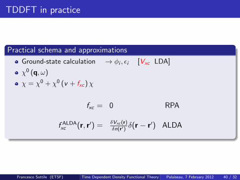
Practical schema and approximations
Ground-state calculation → φi , εi [Vxc LDA]
χ0 (q, ω)
χ = χ0 + χ0 (v + fxc)χ
fxc = 0 RPA
f ALDAxc (r, r′) = δVxc (r)δn(r′)
δ(r − r′) ALDA
Francesco Sottile (ETSF) Time Dependent Density Functional Theory Palaiseau, 7 February 2012 40 / 32
Outline
1 Introduction: why TD-DFT ?
2 (Just) A bit of Formalism - The Boring PartTDDFT: the FoundationLinear Response Formalism
3 TDDFT in practice:The ALDA: Achievements and ShortcomingsThe Quest for the Holy FunctionalNew Frontiers
4 Perspectives and Resources
Francesco Sottile (ETSF) Time Dependent Density Functional Theory Palaiseau, 7 February 2012 41 / 32
ALDA: Achievements and Shortcomings
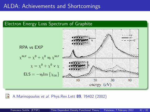
Electron Energy Loss Spectrum of Graphite
RPA vs EXP
χNLF = χ0 + χ0 v0 χNLF
χ = χ0 + χ0 v χ
ELS = −v0Imχ00
A.Marinopoulos et al. Phys.Rev.Lett 89, 76402 (2002)
Francesco Sottile (ETSF) Time Dependent Density Functional Theory Palaiseau, 7 February 2012 42 / 32
ALDA: Achievements and Shortcomings
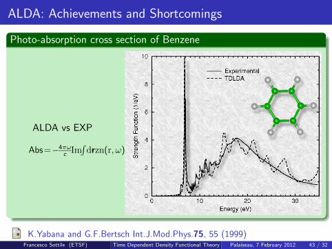
Photo-absorption cross section of Benzene
ALDA vs EXP
Abs=−4πωc Im
∫drzn(r, ω)
K.Yabana and G.F.Bertsch Int.J.Mod.Phys.75, 55 (1999)Francesco Sottile (ETSF) Time Dependent Density Functional Theory Palaiseau, 7 February 2012 43 / 32
ALDA: Achievements and Shortcomings
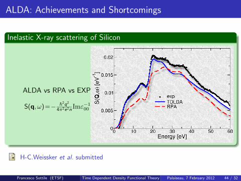
Inelastic X-ray scattering of Silicon
ALDA vs RPA vs EXP
S(q, ω)=− ~2q2
4π2e2n Imε−100
H-C.Weissker et al. submitted
Francesco Sottile (ETSF) Time Dependent Density Functional Theory Palaiseau, 7 February 2012 44 / 32
ALDA: Achievements and Shortcomings
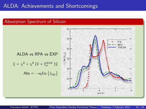
Absorption Spectrum of Silicon
ALDA vs RPA vs EXP
χ = χ0 + χ0 (v + f ALDAxc )χ
Abs = −v0Imχ00
Francesco Sottile (ETSF) Time Dependent Density Functional Theory Palaiseau, 7 February 2012 45 / 32
ALDA: Achievements and Shortcomings
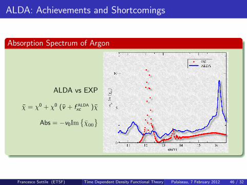
Absorption Spectrum of Argon
ALDA vs EXP
χ = χ0 + χ0 (v + f ALDAxc )χ
Abs = −v0Imχ00
Francesco Sottile (ETSF) Time Dependent Density Functional Theory Palaiseau, 7 February 2012 46 / 32

ALDA: Achievements and Shortcomings
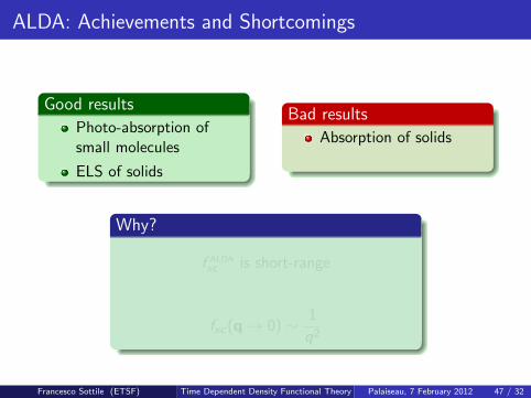
Good results
Photo-absorption ofsmall molecules
ELS of solids
Bad results
Absorption of solids
Why?
f ALDAxc is short-range
fxc(q→ 0) ∼ 1
q2
Francesco Sottile (ETSF) Time Dependent Density Functional Theory Palaiseau, 7 February 2012 47 / 32
ALDA: Achievements and Shortcomings
Good results
Photo-absorption ofsmall molecules
ELS of solids
Bad results
Absorption of solids
Why?
f ALDAxc is short-range
fxc(q→ 0) ∼ 1
q2
Francesco Sottile (ETSF) Time Dependent Density Functional Theory Palaiseau, 7 February 2012 47 / 32

ALDA: Achievements and Shortcomings
Good results
Photo-absorption ofsmall molecules
ELS of solids
Bad results
Absorption of solids
Why?
f ALDAxc is short-range
fxc(q→ 0) ∼ 1
q2
Francesco Sottile (ETSF) Time Dependent Density Functional Theory Palaiseau, 7 February 2012 47 / 32
ALDA: Achievements and Shortcomings
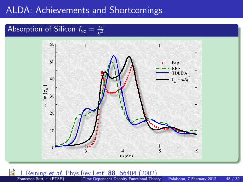
Absorption of Silicon fxc = αq2
L.Reining et al. Phys.Rev.Lett. 88, 66404 (2002)Francesco Sottile (ETSF) Time Dependent Density Functional Theory Palaiseau, 7 February 2012 48 / 32
Outline
1 Introduction: why TD-DFT ?
2 (Just) A bit of Formalism - The Boring PartTDDFT: the FoundationLinear Response Formalism
3 TDDFT in practice:The ALDA: Achievements and ShortcomingsThe Quest for the Holy FunctionalNew Frontiers
4 Perspectives and Resources
Francesco Sottile (ETSF) Time Dependent Density Functional Theory Palaiseau, 7 February 2012 49 / 32

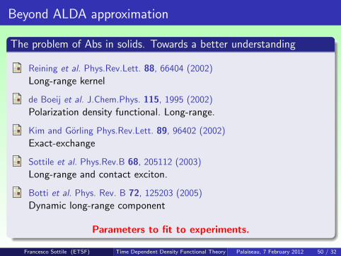
Beyond ALDA approximation
The problem of Abs in solids. Towards a better understanding
Reining et al. Phys.Rev.Lett. 88, 66404 (2002)
Long-range kernel
de Boeij et al. J.Chem.Phys. 115, 1995 (2002)
Polarization density functional. Long-range.
Kim and Gorling Phys.Rev.Lett. 89, 96402 (2002)
Exact-exchange
Sottile et al. Phys.Rev.B 68, 205112 (2003)
Long-range and contact exciton.
Botti et al. Phys. Rev. B 72, 125203 (2005)
Dynamic long-range component
Parameters to fit to experiments.
Francesco Sottile (ETSF) Time Dependent Density Functional Theory Palaiseau, 7 February 2012 50 / 32
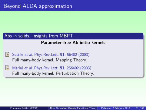
Beyond ALDA approximation
Abs in solids. Insights from MBPT
Parameter-free Ab initio kernels
Sottile et al. Phys.Rev.Lett. 91, 56402 (2003)
Full many-body kernel. Mapping Theory.
Marini et al. Phys.Rev.Lett. 91, 256402 (2003)
Full many-body kernel. Perturbation Theory.
Francesco Sottile (ETSF) Time Dependent Density Functional Theory Palaiseau, 7 February 2012 51 / 32
The Mapping Theory
The idea
BSE works ⇒
we get the ingredients of the BSEand we put them in TDDFT
Francesco Sottile (ETSF) Time Dependent Density Functional Theory Palaiseau, 7 February 2012 52 / 32
The Mapping Theory
The idea
L(1234) = L0GW(1234) + L0GW(1256) [v −W ] L(7834)
χ(12) = χ0(12) + χ0(13) [v + fxc ]χ(42)
fxc =(χ0
GW
)−1GGWGG
(χ0
GW
)−1× still apply GW√
solve 2-point eq. for χ (rather than L)
Francesco Sottile (ETSF) Time Dependent Density Functional Theory Palaiseau, 7 February 2012 53 / 32
The Mapping Theory
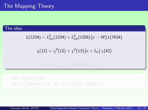
The idea
L(1234) = L0GW(1234) + L0GW(1256) [v −W ] L(7834)
χ(12) = χ0(12) + χ0(13) [v + fxc ]χ(42)
fxc =(χ0
GW
)−1GGWGG
(χ0
GW
)−1× still apply GW√
solve 2-point eq. for χ (rather than L)
Francesco Sottile (ETSF) Time Dependent Density Functional Theory Palaiseau, 7 February 2012 53 / 32

The Mapping Theory
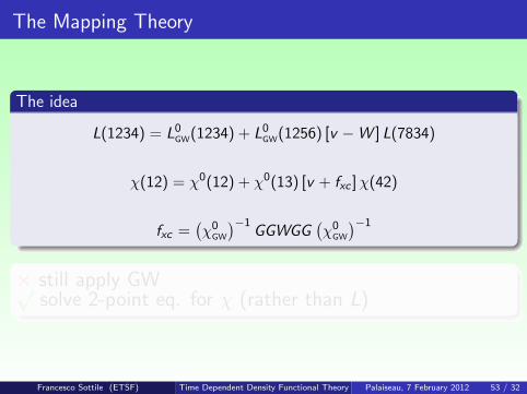
The idea
L(1234) = L0GW(1234) + L0GW(1256) [v −W ] L(7834)
χ(12) = χ0(12) + χ0(13) [v + fxc ]χ(42)
fxc =(χ0
GW
)−1GGWGG
(χ0
GW
)−1× still apply GW√
solve 2-point eq. for χ (rather than L)
Francesco Sottile (ETSF) Time Dependent Density Functional Theory Palaiseau, 7 February 2012 53 / 32
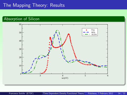
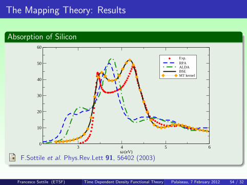
The Mapping Theory: Results
Absorption of Silicon
3 4 5 6ω (eV)
0
10
20
30
40
50
60
Exp.RPAALDA
Francesco Sottile (ETSF) Time Dependent Density Functional Theory Palaiseau, 7 February 2012 54 / 32

The Mapping Theory: Results
Absorption of Silicon
3 4 5 6ω (eV)
0
10
20
30
40
50
60
Exp.RPAALDABSE
Francesco Sottile (ETSF) Time Dependent Density Functional Theory Palaiseau, 7 February 2012 54 / 32
The Mapping Theory: Results
Absorption of Silicon
3 4 5 6ω (eV)
0
10
20
30
40
50
60
Exp.RPAALDABSEMT kernel
F.Sottile et al. Phys.Rev.Lett 91, 56402 (2003)
Francesco Sottile (ETSF) Time Dependent Density Functional Theory Palaiseau, 7 February 2012 54 / 32

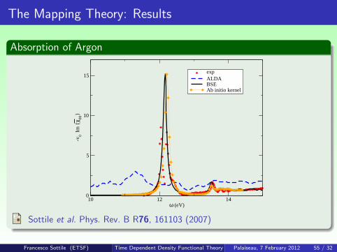
The Mapping Theory: Results
Absorption of Argon
10 12 14ω (eV)
0
5
10
15-v
0 I
m
χ 00
expALDABSE
Francesco Sottile (ETSF) Time Dependent Density Functional Theory Palaiseau, 7 February 2012 55 / 32
The Mapping Theory: Results
Absorption of Argon
10 12 14ω (eV)
0
5
10
15-v
0 I
m
χ 00
expALDABSEAb initio kernel
Sottile et al. Phys. Rev. B R76, 161103 (2007)
Francesco Sottile (ETSF) Time Dependent Density Functional Theory Palaiseau, 7 February 2012 55 / 32
The Mapping Theory: Results
Tested also on absorption of SiO2, DNA bases, Ge-nanowires,RAS of diamond surface, and EELS of LiF.
Marini et al. Phys.Rev.Lett. 91, 256402 (2003).
Bruno et al. Phys.Rev.B 72 153310, (2005).
Palummo et al. Phys.Rev.Lett. 94 087404 (2005).
Varsano et al. J.Phys.Chem.B 110 7129 (2006).
Francesco Sottile (ETSF) Time Dependent Density Functional Theory Palaiseau, 7 February 2012 56 / 32
Spectra of simple systems
TDDFT is the method of choice√
Absorption spectra of solids and simple molecules√
Electron energy loss spectra√
Refraction indexes√
Inelastic X-ray scattering spectroscopy
Francesco Sottile (ETSF) Time Dependent Density Functional Theory Palaiseau, 7 February 2012 57 / 32
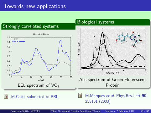
Towards new applications
Strongly correlated systems
0
0.2
0.4
0.6
0.8
1
1.2
1.4
1.6
0 10 20 30 40 50 60ω [eV]
Monoclinic Phase
EXPTDDLA
EEL spectrum of VO2
M.Gatti, submitted to PRL
Biological systems
Abs spectrum of Green FluorescentProtein
M.Marques et al. Phys.Rev.Lett 90,
258101 (2003)
Francesco Sottile (ETSF) Time Dependent Density Functional Theory Palaiseau, 7 February 2012 58 / 32
Outline
1 Introduction: why TD-DFT ?
2 (Just) A bit of Formalism - The Boring PartTDDFT: the FoundationLinear Response Formalism
3 TDDFT in practice:The ALDA: Achievements and ShortcomingsThe Quest for the Holy FunctionalNew Frontiers
4 Perspectives and Resources
Francesco Sottile (ETSF) Time Dependent Density Functional Theory Palaiseau, 7 February 2012 59 / 32
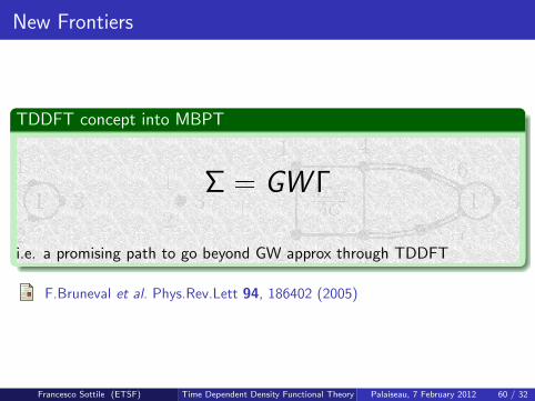
New Frontiers
TDDFT concept into MBPT
Σ = GW Γ
i.e. a promising path to go beyond GW approx through TDDFT
F.Bruneval et al. Phys.Rev.Lett 94, 186402 (2005)
Francesco Sottile (ETSF) Time Dependent Density Functional Theory Palaiseau, 7 February 2012 60 / 32
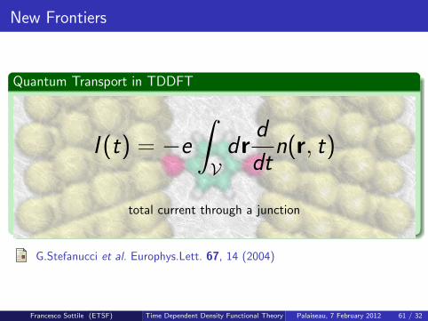
New Frontiers
Quantum Transport in TDDFT
I (t) = −e∫Vdr
d
dtn(r, t)
total current through a junction
G.Stefanucci et al. Europhys.Lett. 67, 14 (2004)
Francesco Sottile (ETSF) Time Dependent Density Functional Theory Palaiseau, 7 February 2012 61 / 32
New Frontiers
Let’s go back to Ground-State
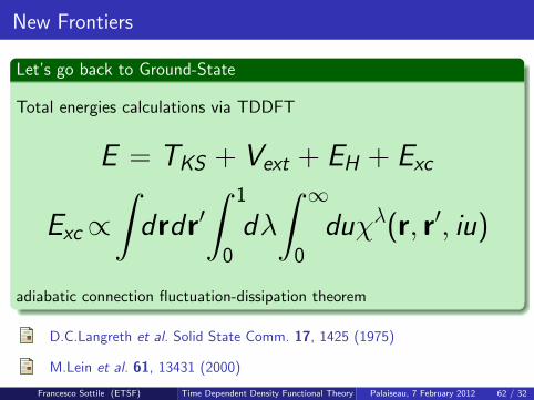
Total energies calculations via TDDFT
E = TKS + Vext + EH + Exc
Exc∝∫drdr′
∫ 1
0
dλ
∫ ∞0
duχλ(r, r′, iu)
adiabatic connection fluctuation-dissipation theorem
D.C.Langreth et al. Solid State Comm. 17, 1425 (1975)
M.Lein et al. 61, 13431 (2000)
Francesco Sottile (ETSF) Time Dependent Density Functional Theory Palaiseau, 7 February 2012 62 / 32

Outline
1 Introduction: why TD-DFT ?
2 (Just) A bit of Formalism - The Boring PartTDDFT: the FoundationLinear Response Formalism
3 TDDFT in practice:The ALDA: Achievements and ShortcomingsThe Quest for the Holy FunctionalNew Frontiers
4 Perspectives and Resources
Francesco Sottile (ETSF) Time Dependent Density Functional Theory Palaiseau, 7 February 2012 63 / 32
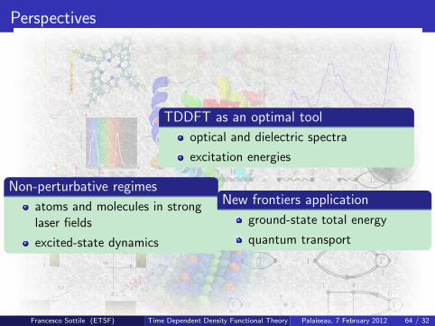
Perspectives
TDDFT as an optimal tool
optical and dielectric spectra
excitation energies
Non-perturbative regimes
atoms and molecules in stronglaser fields
excited-state dynamics
New frontiers application
ground-state total energy
quantum transport
Time-Dependent Density Functional Theory Springer (2006)
Francesco Sottile (ETSF) Time Dependent Density Functional Theory Palaiseau, 7 February 2012 64 / 32
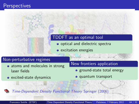
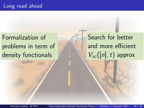
Long road ahead
Formalization of
problems in term of
density functionals
Search for better
and more efficient
Vxc([n], t) approx
Problems
charge transfer systems
double excitations
efficient calculation for solids
Francesco Sottile (ETSF) Time Dependent Density Functional Theory Palaiseau, 7 February 2012 65 / 32
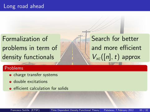
Resources
Codes (more or less) available for TDDFT
Octopus (Marques,Castro,Rubio) -(real space, real time) - finite systems
- GPL
http://www.tddft.org/programs/octopus/
DP (Olevano,Reining,Sottile) - (reciprocal space, frequency domain) -
solides and finite systems - Academic Free License
http://theory.polytechnique.fr/codes/dp/dp.html
Self (Marini) - (reciprocal space, frequency domain)
Fleszar code
Rehr (core excitations)
TDDFT (Bertsch)
VASP, SIESTA, ADF, TURBOMOLE
TD-DFPT (Baroni)
Francesco Sottile (ETSF) Time Dependent Density Functional Theory Palaiseau, 7 February 2012 66 / 32


![Density Functional Theory investigation for Sodium atom on … · 2020-04-01 · case is the spatially dependent electron density [3]. Hence the name density functional theory comes](https://img.pdfslide.net/doc/110x75/5f5af946a114d867551012c7/density-functional-theory-investigation-for-sodium-atom-on-2020-04-01-case-is.jpg)


![Excited states from time-dependent density functional theorykieron/dft/pubs/EBF07.pdfOn the other hand, time-dependent density functional theory (TDDFT)[11{15] applies the same philosophy](https://img.pdfslide.net/doc/110x75/600933e833b2a871117fcf79/excited-states-from-time-dependent-density-functional-theory-kierondftpubsebf07pdf.jpg)