Journal o f Statistical Physics, Vol. 68, Nos. 5/6, 1992

Time-Dependent Thermodynamic Properties of the Ising Model from Damage Spreading

Sharon C. Glotzer, 1 Peter H. Poole, 1 and N a e e m Jan 2

Received February 7, 1992

The relationship between damage spreading and static thermodynamic proper- ties in the Ising model developed by Coniglio et al. is here extended to include time-dependent thermodynamic quantities. We exploit this new result to measure the time-dependent spin correlation function from damage spreading in the Ising model with heat bath and Glauber dynamics. Until now, only static thermodynamic quantities have been correctly determined from damage spreading, and even then, only with heat bath dynamics. We also show that there are significant differences between the kinetics of damage spreading as found in heat bath and Glauber dynamics.

KEY WORDS: Ising problems; dynamics; damage spreading.

1. I N T R O D U C T I O N

Damage spreading is a useful method for detecting the onset of so-called chaotic behavior in cellular automata/1-3) and has also been applied to thermal systems evolving via nondeterministic dynamics./4 23) The damage spreading method consists of starting with two systems, identical in all respects apar t from some localized initial perturbation, and noting the distance between the systems in configurat ion space as the systems evolve with the same rules and constraints. In this way, the sites which are correlated at a specific instant to a given site as the damage evolves to its equilibrium state can be directly pinpointed. In the Ising model, Coniglio e t al. ~8~ (referred to in the following as C A H J ) observed that there were two types of damage possible, and that static thermodynamic properties are

1Center for Polymer Studies and Physics Department, Boston University, Boston, Massachusetts 02215.

2 Physics Department, St. Francis Xavier University, Antigonish, Nova Scotia, Canada B2G 1CO.

895

822/68/5-6-15 0022-4715/92/0900-0895506.50/0 �9 1992 Plenum Publishing Corporation

896 Glotzer e t al.

related to the difference between the probabilities for finding each type of damage.

In this paper we extend the formalism of CAHJ and relate the time evolution of this "damage difference" to the time-dependent spin correla- tion function. We make three points:

1. There exists an exact relation between the quantities measured in damage spreading and time-dependent thermodynamic properties.

2. Damage spreading correctly gives thermodynamic properties for dynamics other than heat bath. That this should be true was proven by CAHJ, but it has never (to our knowledge) been confirmed in simulation, a fact which has perhaps generated the false impression that damage spreading is only related to thermodynamic properties in the special case of heat bath dynamics. An underlying purpose of the present work is to emphasize that damage spreading is a general tool that may be applied to any lattice system of binary variables (and perhaps to a wider class of systems) using any dynamics.

3. We show in the last section that damage spreading is not simply a new way to evaluate properties that can be measured by other means. We will describe fundamental differences in the way that damage spreads in Glauber dynamics as compared to heat bath dynamics. This is important because it shows that damage spreading can be used to probe the microscopic process of the propagation of correlations as seen in a par- ticular dynamics, and that two dynamics that give the same equilibrium thermodynamic results may carry out this process in starkly different ways.

2. RELATION BETWEEN D A M A G E SPREADING A N D THE T I M E - D E P E N D E N T SPIN CORRELATION FUNCTION

In this section we establish a general relationship between the damage spreading process and the time-dependent spin correlation function C(i, t), defined as the probability for a spin at site i at time t to be in the same state as that of the spin at the origin at time t = 0.

Consider a computer simulation of a large Ising system of linear size 2L + 1 in dimension d. The system is in equilibrium at temperature T and is subject to an external magnetic field h. (For concreteness, we address here the Ising model, but note that all of the formalism that we develop in this section applies to any lattice system of binary variables with a well- defined distribution of equilibrium states.) In general we consider the system to be in an arbitrary initial equilibrium spin configuration {a } and to evolve via some arbitrary dynamical rules which keep it in equilibrium.

We now select an equilibrium configuration {o-} of the system, and

Damage Spreading 897

call this the configuration at t = 0. At time t = 0 we clone the system into two identical copies A and B. System A is then modified by permanently fixing its central spin (at site i = 0) to its value at t = 0 for all subsequent evolution of A. System B is not altered. Systems A and B are then each evolved. In general, the two systems may be evolved with different dynamics and/or using different sequences of random numbers to update their spins. As the systems are evolved, their respective spin configurations, initially identical, may become different due to the constraint on the central spin in A. "Damage spreading" is the specific process by which these configurations become different over time, as monitored by a spin-by-spin comparison of the two systems as they evolve.

To quantify the comparison of the spin configurations of A and B, we adopt the following terminology. Define ~r,A(t) to be the value of the spin variable at site i in system A at time t. The value of this spin can be either 1 o r - 1 . The permanently fixed central spin in A then has the value a~ ( t )=~J (0 ) for all t~>0. Call d+-(i,t) the probability to find the following kind of damage at site i at time t: that aA(t)=a~(0) while a ~ ( t ) = - a J ( 0 ) . Similarly, do+(i, t) is the probability to find a~(t) = --aoA(0) and a~(t)= aA(0). Following CAHJ, we can then define the following quantity, which we call the "time-dependent damage difference":

Fo(i, t ) - d ~ (i, t ) -do+(i , t) (2.1)

The subscript 0 indicates that the kind of damage, i.e., either (+ - ) or ( - +) , is determined with respect to the value of the fixed central spin in A.

Let us now define two quantities ~A(t) and ~ ( t ) from which we can construct a function that will give the probabilities d ~ - ( i , t) and d o +(i, t) when averaged over the configurations generated during the simulation. For this purpose, note that when there is (+ - ) damage at site i at time t, the quantity

1 A A gA(t) = 5~o (0)[ao (0) + ~ ( t ) ] (2.2)

is unity, while

1 A A B ~ ( t ) = ~ o (0)[ao (0) + ~i (t)] (2.3)

is zero. Similarly, when there is ( - + ) damage at i at time t, ~ ( t ) = 0 and ~ ( t ) = 1. As desired, the values of the quantities defined in Eqs. (2.2)-(2.3) can therefore be averaged to evaluate

d~- (i, t )= (~A(t)[1 - - ~ ( t ) ] ~ o (2.4)

898

and

Glotzer et aL

d o + (i, t) = <~f(t)[1 - ~za(t)] >0 (2.5)

where <.-. >o denotes an average over an ensemble of systems, each of which is produced by the damage spreading process after a time t, as described above. Substituting (2.4) and (2.5) into (2.1) gives

to( i , t )= ( r c A ( t ) [ I - rCf(t)] >0-- (TCf(t)[ l -- 7C~(t)] >0 (2.6)

or, equivalently,

Fo(i, t ) = <~A(t) > o -- <nf(t)>o (2.7)

Note that, from (2.2)-(2.3),

<T[~(t)> - - _1 1 A O~(I) o-2+~<~ >o (2.8)

and

1 A < ~f(t)>o = �89 + ~<Oo (o) of(t)>o (2.9)

Invoking the condition that a~(0)= o~(t) for all t in (2.8) allows us to rewrite this quantity at a single time, thereby removing the time-dependent character of this quantity: in equilibrium, (o~(t)oA(t)>o is constant with respect to time and equal to the time-independent quantity A A (OOOi >o" The condition that aoS(0)= oA(0), applied to (2.9), removes explicit reference to system A. These conditions together transform (2.8)-(2.9) into

< T c A ( t ) > o = � 8 9 l a a ~<%ai >o (2.10)

and

<~f(t)>o = �89 �89 of(t)>o (2.11)

Substition into (2.7) gives

to(i, t)= �89 <~JOf >o- <o((O) of(t)>o] (2.12a)

We now relate the average ( . . . >o, in which a spin is fixed in A, to the usual unconstrained ensemble average, denoted by <. . . >. Since there are no constrained spins in B and the second term in (2.12a) refers only to B, we can trivially replace ( . . . >o with ( . - . > in that term. Since the first term is a static term, we can apply the time-independent argument given in CAHJ. Their analysis shows that the strength of the static correlation between the central site and the site i, when the central spin is fixed during

Damage Spreading 899

the time average over the trajectory in phase space generated by the dynamics, is proportional to the strength of the static correlation when the central spin is not fixed. In CAHJ, because they always fix the central spin "up," a constant of proportionality is needed to account for the fact that they therefore only sample a fraction of phase space. Since our damage definition allows the central spin to be fixed either "up" or "down" in accordance with the spin state equilibrium probabilities, we can avoid this prefactor by averaging over independent trajectories. Hence, in the present analysis, the average strength of the static correlation to the central site is exactly the same regardless of whether or not the central spin is fixed. We therefore conclude that for the purpose of measuring the static correlation function, which is calculated from A a (~roa ~ ), the constrained ensemble average is an equivalent representation of the unconstrained ensemble average. Consequently, we rewrite (2.12a) as

Co(i, t )= �89 ) - (~g(0) a f ( t ) ) ] (2.12b)

Furthermore, since each term refers to an independent system, we can drop the superscripts A and B. We have, finally,

Fo(i, t )= l [ ( a o a i ) - (ao(0) ~ i ( t ) ) ] (2.12c)

In this notation, the time-dependent correlation function is defined as

(,7o(O) o-~(t)) - (,~)~ C(i, t )= ( a 2 ) _ (~r) 2 (2.13)

whereas the time-independent correlation function C(i, O) is just the value of C(i, t) at t = O:

( a o O ' i ) - ( o - ) ~ C(i, 0 ) - ( -~--k--g~-g (2.14)

Using (2.12)-(2.14), we can therefore form the final relation

2Fo(i , t) C(i, t)= C(i, 0) ( a 2 ) _ Qr)2 (2.15)

Note from (2.12c) that as t o o o, (a0(0) a i ( t ) ) - - , ( a ) 2, so that Fo(i, t) becomes a constant Fo(i, oo) with respect to time, which is propor- tional to the static correlation function C(i, 0). In this limit, C(i, t) = 0, and the relation in (2.15) reduces to

2Fo(i, oo ) C(i, 0 ) - (o.2) _ (o.) 2 (2.16)

900 Glotzer et al.

which is similar in form to a relation derived for static quantities in CAHJ. The important difference between the result in (2.15) and (2.16), and the result in CAHJ, is that we have used a modified definition of damage. In CAHJ, the damage is defined with respect to a central spin which is always permanently fixed "up" in the A system at t = 0, regardless of its original orientation; in this work, the central spin in A is fixed permanently to be in whatever spin state it happens to be in at t = 0. In order to derive a time- dependent relation for damage spreading, we found it more convenient to consider this latter, modified definition.

It is also important to note that at no point in the above analysis was it required that the systems A and B be evolved with the same dynamics, or random number sequences. Yet it is found that it is still an advantage to do so, since this procedure ensures that all damage arises solely from the initial damage. Other sources of differences between the two systems are suppressed when identical updating schemes are used. This is an advantage because, as we will show in the last section, comparing how damage spreads in different Monte Carlo algorithms, when the damage is due solely to the initial damage, provides a very sensitive test of the differences between two such dynamics. However, even though it is therefore customary to use the same updating scheme in both of the cloned systems in a damage spreading study, it is important to remember that this is not necessary for evaluating thermodynamic quantities from the measurement of damage.

3. D A M A G E S P R E A D I N G IN HEAT BATH A N D G L A U B E R D Y N A M I C S

In this section, we describe a damage spreading study of the d = 2 Ising model evolving via both heat bath and Glauber dynamics. Specifi- cally, we calculate the time-dependent spin correlation functions as defined in (2.13) at criticality, both directly and via the damage difference Fo(i, t) for both dynamics. The purpose is to confirm that the analysis in Section 2 is correct, i.e., that we can in fact obtain time-dependent thermodynamic properties from damage spreading, and, as motivated in the Introduction, we want to demonstrate that in general, damage spreading also correctly gives thermodynamic properties for a dynamics other than heat bath.

The difference between these two dynamics appears in the way that individual spins are updated during a timestep. In heat bath dynamics, a spin at site i is set "up" with a probability given by

exp(Jhi) P~P - (3.1)

exp( - Jk i ) + exp(Jh,)

Damage Spreading 901

where J = J/kB T, J is the ferromagnetic interaction energy between nearest neighbor spins, kB is Boltzmann's constant, and T is temperature, and h i i = Z j aj, where the sum is taken over nearest neighbors of i only. In Glauber dynamics, spins are flipped with a probability given by

nip _ e x p ( - J a i h i ) Pi - (3.2)

exp(Jaihi) + exp(-Jcr ihi)

where cr i is the value of the spin at site i. For both dynamics, the computational scheme is as follows. We

simulate a two-dimensional Ising model at T = T c in a system of linear size 2 L + 1=31. After equilibrating for a sufficient number of Monte Carlo time steps (MCS), we make a copy of the system, giving two identical spin lattices A and B. Damage is initiated at t = 0 by permanently fixing the central spin in lattice A. The simulation is then continued using the same random numbers to update corresponding sites on the two lattices. Since we have damaged the central site, the damage will spread through the system starting from the center.

To measure Fo(i, t), each time a site is updated after t = 0 a variable associated with the site i and time t is assigned a value according to the state of the damage on that site at that time: + 1 if the site is damaged (+ - ), - 1 if the site is damaged ( - + ), and 0 if there is no damage. After many realizations (i.e., begin with a new equilibrated system, clone, initiate damage, and observe for a time t) of the damage spreading from the central site, each starting from different equilibrium spin configurations, an estimate for Fo(i, t) is obtained by averaging the value of the variable associated with site i at time t over all of the realizations performed. For the heat bath system, 13,635 realizations were performed, while for the Glauber system, 29,654 realizations were performed. In addition, Fo(i, t) for the set of sites at a distance r from the origin can be averaged to give Fo(r, t). For comparison, the spin correlation function C(r, t) is also found directly by calculating the usual thermal averages, as indicated in (2.13).

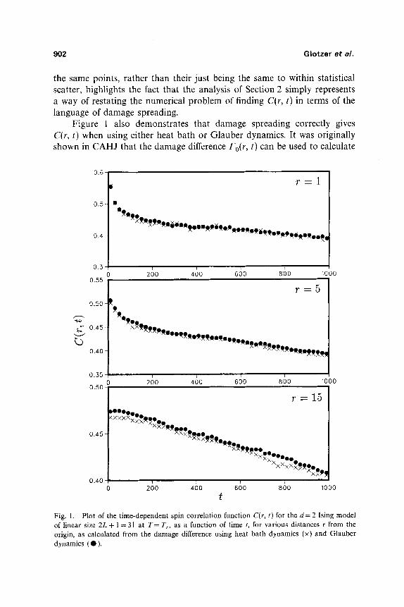
The results of these simulations are shown in Fig. 1, where for both dynamics C(r, t) is plotted as a function of time t, for several values of the distance from the origin r. We find first that for both heat bath and Glauber dynamics, the values calculated for C(r, t) from the damage dif- ference F(r, t) are identical to those values obtained directly from the spin states. The values plotted in Fig. 1 were found from the damage difference via (2.15), where system A was used to calculate C(i, 0); the points for C(r, t) found directly via (2.13), using system B only, fall on exactly the same points. This correspondence confirms the analysis of the previous section. Indeed, given that the two ways of calculating C(r, t) give exactly

902 Glotzer et al.

the same points, rather than their just being the same to within statistical scatter, highlights the fact that the analysis of Section 2 simply represents a way of restating the numerical problem of finding C(r, t) in terms of the language of damage spreading.

Figure 1 also demonstrates that damage spreading correctly gives C(r, t) when using either heat bath or Glauber dynamics. It was originally shown in CAHJ that the damage difference Fo(r, t) can be used to calculate

0 6

0 5

0 4

r = l

I I

0 . 5 0 2 0 0 4 0 0 6 0 0 8 0 0 1 0 0 0

0 . 5 5 ~"

o.50 ~ r = 5

i iit " . ~ . '"xx,,,,.,...,,,.,,,..,..,.,. 0 . 5 5 ! ~ ~ ~ ,

0 2 0 0 4 0 0 6 0 0 8 0 0 1 0 0 0 0 . 5 0 -

0 . 4 5 -

0.40

r = 15 DQOO~-- <xxx~OOmoo

A X X ~ X O 0 X x x ~ o o o _

•215215 ~ x X x x x ~ o o _

XX~q

0 200 400 600 800 1000

t

Fig. 1. Plot of the time-dependent spin correlation function C(r, t) for the d = 2 Ising model of linear size 2 L + 1 = 3 1 a t T = To, as a f u n c t i o n o f t i m e t, for various distances r from the origin, as calculated from the damage difference using heat bath dynamics (x) and Glauber dynamics ( �9 ).

Damage Spreading 903

thermodynamic quantities for any dynamics, but to our knowledge, this is the first demonstration of the validity of damage spreading for measuring thermodynamic quantities when a dynamics other than heat bath has been used. The reason that heat bath is used almost exclusively in damage spreading studies is that, as shown in CAHJ, in heat bath dynamics there is no possibility of ever generating ( - + ) damage, and therefore d o + (i, t) is always zero for all i and t. In this circumstance, (2.1) reduces to

Fo(i, t ) = do ~ (i, t) (3.3)

For heat bath dynamics, then, the damage difference Fo(i, t) is trivially equal to the "damage sum" f20(i, t), defined as

(2o(i , t ) = d g - ( i , t) + do+(i, t) (3.4)

This damage sum is simply related to the average number of damaged spins in the system (H(t)) :

( e ( t ) ) =y~ ~0(i, t) (3.5) i

a quantity known both as the "average total damage" and the "average Hamming distance." In general, the damage sum is easier to calculate than the damage difference, since it does not require a discrimination of what type of damage is on a particular site. Heat bath dynamics has typically been the dynamics of choice in damage spreading studies because in heat bath dynamics, since Fo(i, t)= s t), the damage sum can also be used to calculate thermodynamic data, and an instantaneous image of the damage represents an image of the specific sites correlated to the central damaged site. However, as we will show in the next section, we have found that comparing how damage spreads in different dynamics offers a sensitive way to explore how such dynamics differ.

We note that a systematic deviation in C(r, t) between heat bath and Glauber dynamics seems to exist near the boundary (see Fig. 1, r = 15). This may indicate a difference in the way that boundary and/or lattice effects manifest themselves in the different dynamics.

We also note that we have measured the damage difference with the appropriate boundary conditions to find the magnetization as suggested in CAHJ. For T< Tc with Glauber dynamics, we find values of the magnetization within numerical error of those obtained from the exact solution of Onsager. This again confirms that damage spreading gives the correct thermodynamic properties of the Ising model even when using Gtauber dynamics.

904 Glotzer e t al.

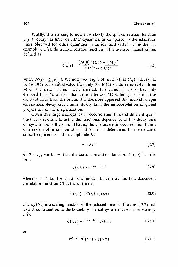
Finally, it is striking to note how slowly the spin correlation function C(r, t) decays in time for either dynamics, as compared to the relaxation times observed for other quantities in an identical system. Consider, for example, Ca4(t), the autocorrelation function of the average magnetization, defined as

(M(O) M(t)) - ( M ) 2 C.M(t) = ( M 2 ) _ ( M ) 2 (3.6)

where M(t)= Zi cry(t). We note (see Fig. 1 of ref. 21) that Ca4(t) decays to below 10% of its initial value after only 500 MCS for the same system from which the data in Fig. 1 were derived. The value of C(r, t) has only dropped to 85% of its initial value after 500 MCS, for spins one lattice constant away from the origin. It is therefore apparent that individual spin correlations decay much more slowly than the autocorrelation of global properties like the magnetization.

Given this large discrepancy in decorrelation times of different quan- tities, it is relevant to ask if the functional dependence of this decay time on system size is the same. That is, the characteristic decorrelation time of a system of linear size 2L + 1 at T = Tc is determined by the dynamic critical exponent z and an amplitude K:

~ KL: (3.7)

At T = To, we know that the static correlation function C(r, 0) has the form

C(r,O)~r -{a 2+.~ (3.8)

where r/= 1/4 for the d = 2 Ising model. In general, the time-dependent correlation function C(r, t) is written as

C(r, t ) ~ C(r, O)f(t/r) (3.9)

wheref(t/T) is a scaling function of the reduced time t/r. If we use (3.7) and restrict our attention to the boundary of a subsystem at L = r, then we may write

C(r, t )~ r (a-2+")f(t/rZ) (3.10)

o r

ra- 2 +"C(r, t )~ f ( t / r z) (3.11)

Damage Spreading 905

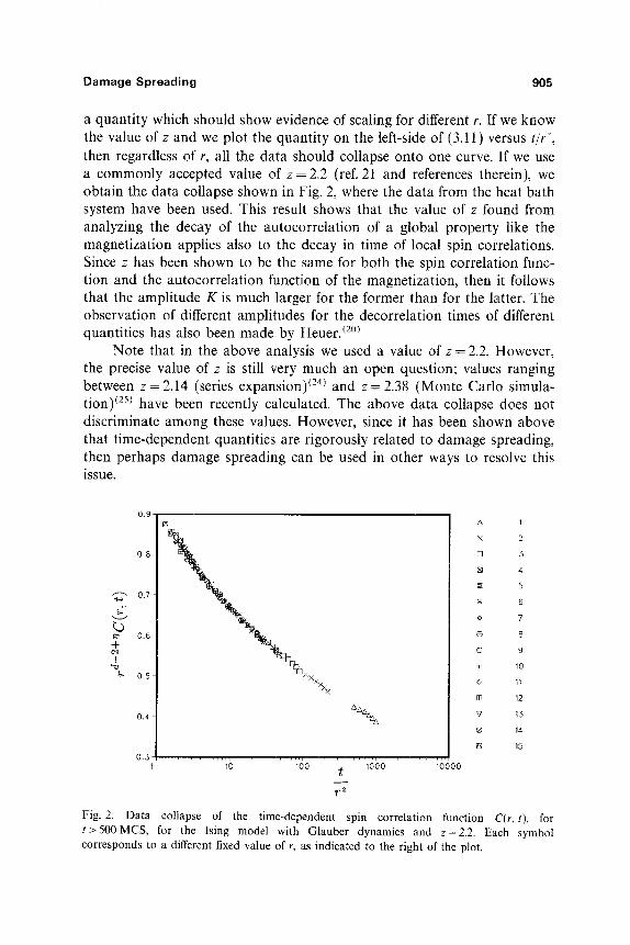
a quantity which should show evidence of scaling for different r. If we know the value of z and we plot the quantity on the left-side of (3.11) versus t/r z, then regardless of r, all the data should collapse onto one curve. If we use a commonly accepted value of z = 2.2 (ref. 21 and references therein), we obtain the data collapse shown in Fig. 2, where the data from the heat bath system have been used. This result shows that the value of z found from analyzing the decay of the autocorrelation of a global property like the magnetization applies also to the decay in time of local spin correlations. Since z has been shown to be the same for both the spin correlation func- tion and the autocorrelation function of the magnetization, then it follows that the amplitude K is much larger for the former than for the latter. The observation of different amplitudes for the decorrelation times of different quantities has also been made by Heuer. (2~

Note that in the above analysis we used a value of z = 2.2. However, the precise value of z is still very much an open question; values ranging between z = 2.14 (series expansion) (24) and z = 2.38 (Monte Carlo simula- tion) (25) have been recently calculated. The above data collapse does not discriminate among these values. However, since it has been shown above that time-dependent quantities are rigorously related to damage spreading, then perhaps damage spreading can be used in other ways to resolve this issue.

0.9-

0 .8

0.7 �84

~" 0.6 +

0 . 5 -

0.4

0.3 ........ E ........ , ........ , ........

10 100 ~ 1000 1 0 0 0 0

/ , z

I

x 2

[] 3

[] 4

5

6

@' 7

| 8

o 9

+ 10

o I~

[] 12

v 13

| 14

[] 15

Fig. 2. Data collapse of the time-dependent spin correlation function C(r,t), for t>500MCS, for the Ising model with Glauber dynamics and z=2.2. Each symbol corresponds to a different fixed value of r, as indicated to the right of the plot.

906 Glotzer e t al.

4. THE MICROSCOPIC PROCESS OF D A M A G E SPREADING

In simulating thermal systems, various dynamics are often used inter- changeably because they give the same equilibrium results. For example, Swendsen-Wang, Kawasaki, heat bath, and Glauber dynamics are com- mon Monte Carlo computer algorithms used to simulate the Ising model. In choosing a particular dynamics, practicalities such as computational speed and efficiency can dictate the choice of algorithm as long as one is interested only in static equilibrium phenomena, such as measuring the susceptibility, specific heat, or critical exponents.

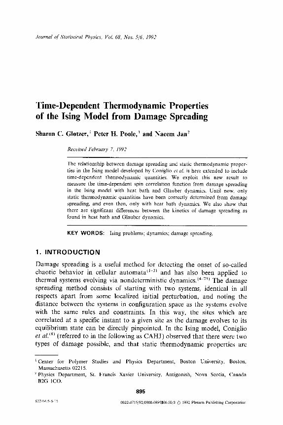
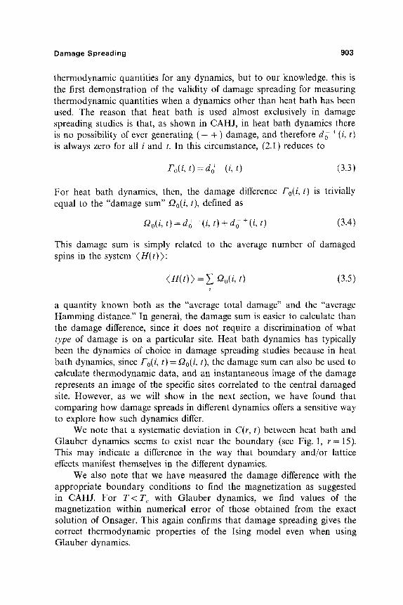
Fig. 3.

t~.

va

(a)

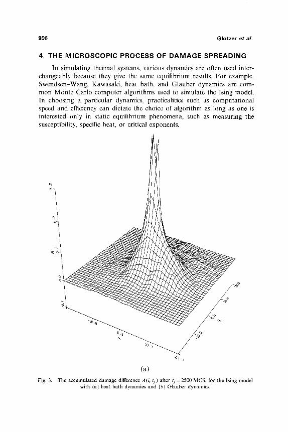
The accumulated damage difference A(i, tj) after If-- 2500 MCS, for the Ising model with (a) heat bath dynamics and (b) Glauber dynamics.

Damage Spreading 907

w.

1 Q . Q ~

~0, 0

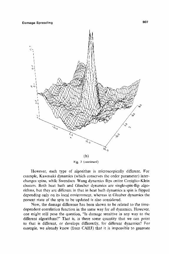
(b) Fig. 3 (continued)

However, each type of algorithm is microscopically different. For example, Kawasaki dynamics (which conserves the order parameter) inter- changes spins, while Swendsen-Wang dynamics flips entire Coniglio-Klein clusters. Both heat bath and Glauber dynamics are single-spin-flip algo- rithms, but they are different in that in heat bath dynamics a spin is flipped depending only on its local environment, whereas in Glauber dynamics the present state of the spin to be updated is also considered.

Now, the damage difference has been shown to be related to the time- dependent correlation function in the same way for all dynamics. However, one might still pose the question, "Is damage sensitive in any way to the different algorithms?" That is, is there some quantity that we can point to that is different, or develops differently, for different dynamics? For example, we already know (from CAHJ) that it is impossible to generate

908 Glotzer e t al.

( - + ) damage with heat bath dynamics, while both types of damage are possible with Glauber dynamics. This can be understood by examining the probabilities with which spins are either flipped or put "up" in Glauber or heat bath dynamics, respectively.

By similar consideration of the conspiracy of updating probabilities, we can understand the following observations:

1. In a Glauber system, where one can have both (+ - ) and ( - + ) damage, ( - + ) damage cannot be created at a site unless that site was damaged in the previous time step and surrounded by both + and - spins.

2. Damage tends to generate its own kind: (+ - ) damage tends to generate more ( + - ), while ( - + ) tends to generate more ( - + ). Because of this, damage spreads through a Glauber system in somewhat separate but contiguous patches of ( + - ) and ( - + ) damage.

3. At any time, damage may heal, but in a Glauber system it is more likely for damage to generate even more damage than to heal, compared with heat bath. The result is that damage is more robust in Glauber dynamics than it is in heat bath, and spreads through the system more quickly.

4. In both dynamics, damage tends to spread at the cluster bound- aries, and remains constant when isolated inside a large Ising cluster; when the cluster boundary diffuses toward the damage patch, the damage undergoes a growth spurt until it runs out of boundary again. This phenomenon seems even more pronounced in heat bath systems, and may contribute to the slow diffusion of the damage through the system at the critical point. Furthermore, this phenomenon may in fact be related to the "metastability" observed by Stanley etal. in Glauber systems. (5) They observed that, at To, damage sometimes got "stuck" and remained frozen for thousands of time steps before spreading again. Since we now know that damage prefers a cluster boundary to spread, this metastability may have been nothing more than a reflection of the time it takes for cluster boundaries to diffuse at To.

5. The most striking difference between the kinetics of damage spreading in Glauber and heat bath is that with Glauber dynamics the damage diffuses through the system much more quickly than in heat bath. Figures 3a and 3b show A(i, tF), the accumulated value of Fo(i, t), defined a s

1 tz A(i, t f ) = t ~ F~ t) (4.1)

t = 0

Damage Spreading 909

Figures 3a and 3b are surface plots of A(i, ts) for a heat bath and Glauber system, respectively, in which the damage spreading in both systems was initiated from the same equilibrium spin configuration and evolved for t~=2500 MCS. We see from these pictures that after 2500 MCS, the damage has long since reached the edges of the Glauber system, but just barely so in the heat bath system. In fact, the characteristic time for the damage to reach the boundary appears to scale linearly with system size L in Glauber dynamics, (22) but scales in the heat bath system (21) as L z. In the heat bath system, because the actual damage is the correlation function, the damage [and hence A(i, tf)] must be zero anywhere C(r, t) is zero. There- fore, the structure of the correlation function emerges smoothly in the center of the heat bath system without influencing regions farther from the center until necessary. In the Glauber system the damage quickly spreads over the whole system, but only gives information about the correlation function within a distance from the origin commensurate with how far the actual spin correlation information has spread in the given time. The conse- quence of this is surprising: These two dynamics propagate correlations with the same time dependence on system size, but in two totally different ways. For example, we know that at early times the correlation function far from the center must be zero. However, there are two ways for this to be true from the point of view of the damage difference: Fo(i, t) may be identically zero in all damage configurations or may average to zero over the ensem- ble of damage configurations. Indeed, in heat bath dynamics, where the damage has not yet reached the outer regions of the system, the correlation function, and therefore A(i, tr), are identically zero. On the other hand, in Glauber dynamics, where both types of damage reach the boundaries rather quickly, the correlation function must average to zero around the fluctuations indicated in Fig. 3b. This serves to emphasize the importance of studying the damage difference when asking thermodynamic questions: in general, the damage sum tells us nothing about the flow of information through the system.

5. C O N C L U S I O N S

We have extended the formalism of CAHJ, which relates damage to thermodynamic quantities, to include time-dependent phenomena. We are in general thus able to observe the spread of correlations in spin systems as visualized by damage spreading. We also observe that the time-depen- dent spin correlation function decays with a characteristic time which is much longer than the characteristic decay time of the magnetization

910 Glotzer et al.

autocorrelation function. A surprising feature of damage spreading is that the microscopic spreading process is very different for heat bath and Glauber dynamics.

A C K N O W L E D G M E N T S

We thank A. Coniglio, H. Gould, G. Huber, W. Klein, K. MacIsaac, P. Slinky, H.E. Stanley, D. Stauffer, and P. Tamayo for their damaging insights. Also, we acknowledge the cooperation of the Boston University Center for Computational Science and the Boston University Academic Computing Center. This work was funded in part by grants from NSF and NSERC of Canada.

REFERENCES

1. S. A. Kaufmann, J. Theor. Biol. 22:437 (1969); Sci. Am. (1991). 2. D. Stauffer, Phil Mag. B 56:901 (1987). 3. S. C. Glotzer, D. Stauffer, and S. Sastry, Physica A 164:1 (1990). 4. U. M. S. Costa, J. Phys. A: Math. Gen. 20:L583 (1987). 5. H. E. Stanley, D. Stauffer, J. Kertesz, and H. J. Herrmann, Phys. Rev. Lett. 59:2326 (1987). 6. G. Le Caer, J. Phys. A 22:L647 (1989); Physica A 159:329 (1989). 7. B. Derrida and G. Weisbuch, Europhys. Lett. 4:657 (1987). 8. A. Coniglio, L. de Arcangelis, H. J. Herrmann, and N. Jan, Europhys. Lett. 8:315 (1989). 9. L. de Arcangelis, H. J. Herrmann, and A. Coniglio, J. Phys. A- Math. Gen. 23:L265 (1990).

10. A. U. Neumann and B. Derrida, J. Phys. (Paris) 49:1647 (1988). 11. L. de Arcangelis, A. Coniglio, and H. J. Herrmann, Europhys. Lett. 9:749 (1989). 12. A. Coninglio, in Correlations and Connectivity, H.E. Stanley and N. Ostrowsky, eds.

(Kluwer, Dordrecht, 1990). 13. H. R. da Cruz, U. M. S. Costa, and E. M. F. Curado, J. Phys. A: Math. Gen. 22:L651

(1989). 14. A. M. Mariz, H. J. Herrmann, and L. de Arcangelis, J. Stat. Phys. 59:1043 (1990). 15. D. Stauffer, Physica A 162:27 (1990). 16. A. M. Mariz and H. J. Herrmann, J. Phys. A: Math. Gen. 22:L1081 (1989). 17. O. Golinelli and B. Derrida, J. Phys. (Paris) 49:1663 (1988). 18. S. S. Manna, J. Phys. (Paris) 51:1261 (1990). 19. M. N. Barber and B. Derrida, J. Stat. Phys. 51:877 (1988). 20. H. O. Heuer, Phys. Worm 1992 (January):23; and preprints. 21. P. H. Poole and N. Jan, J. Phys. A: Math. Gen. 23:L453 (1990). 22. S. C. Glotzer and N. Jan, Physica A 173:325 (1991). 23. H. J. Herrmann, in The Monte Carlo Method in Condensed Matter Physics, K. Binder, ed.

(Springer-Verlag, Berlin, 1991). 24. J. D. Reger, private communication. 25. N. Jan and D. L. Hunter, private communication.