Time-domain numerical computation of noise reduction …aancl.snu.ac.kr/aancl/research/International Journal/[2003... · Time-domain numerical computation of noise reduction by

JOURNAL OFSOUND ANDVIBRATION

www.elsevier.com/locate/jsvi

Journal of Sound and Vibration 268 (2003) 385–401

Time-domain numerical computation of noise reduction bydiffraction and finite impedance of barriers

Chang Woo Lim, Cheolung Cheong, Seong-Ryong Shin, Soogab Lee*

Institute of Advanced Aerospace Technology, School of Mechanical and Aerospace Engineering, Seoul National

University, Seoul 151-742, South Korea

Received 25 June 2001; accepted 21 November 2002

Abstract

A new time-domain numerical method is presented for the estimation of noise reduction by thediffraction and finite impedance of barriers. High order finite difference schemes conventionally used forcomputational aeroacoustics, and time-domain impedance boundary conditions are utilized for thedevelopment of the time-domain method. Compared with other methods, this method can be applied moreeasily to the problems related to nonlinear noise propagation such as impulsive noise and broadband noise.Linearized Euler equations in Cartesian co-ordinates are considered and solved numerically. Straight andT-shaped barriers with and without surface admittance are calculated. In order to assess the accuracy ofthis time-domain method, comparison with the results of SYSNOISE software (Ver. 5.3) are made. Thereare very good agreements between the results of the present time-domain numerical method and theboundary element method of the SYSNOISE software.r 2002 Elsevier Science Ltd. All rights reserved.

1. Introduction

The increasing magnitude and types of noise generated by road traffic in modern city life havearoused much interest in the problem of noise pollution, initiating the development of numericaltechniques and simulations concerned with noise reduction measures. One of the simplest andmost effective measures in open space is a suitably shaped and placed absorbing acoustic barrier.Many methods have been presented to predict the performance of the noise barriers. They can beclassified into three categories, namely, scale-model or full-scale experiments, theoreticalapproaches, and wave-based numerical methods.

ARTICLE IN PRESS

*Corresponding author. School of Mechanical and Aerospace Engineering, Seoul National University, San 56-1,

Shilim-Dong, Kwanak-Gu, Seoul 151-742, South Korea. Tel.: +82-2-880-7384; fax: +82-2-887-2662.

E-mail address: [email protected] (S. Lee).

0022-460X/03/$ - see front matter r 2002 Elsevier Science Ltd. All rights reserved.

doi:10.1016/S0022-460X(02)01534-1

Experimental approaches are often used to solve the practical problems including atmosphericconditions and complex interactions. Scholes et al. [1] performed an experiment with full-scalebarriers on grass-covered ground. May and Osman [2] examined a number of new barrier modelspromising improved performance using a 1/16 scale model experiment. Experimental approaches,however, are more expensive than analytic and numerical methods.

Numerous theoretical techniques have been developed for the prediction of the performance ofthe noise barriers. Many of them are based on geometrical ray theory and the diffraction theory ofacoustic waves extended from the optical diffraction theory. These techniques are based on energymethods and thus ignore phase difference. One of the simplest and most widely used methods isMaekawa’s empirical diffraction model [3] that provides the insertion loss due to a thin-wallbarrier in terms of the Fresnel number. Kawai et al. [4] developed a simple, approximateexpression for Bowman and Senior’s formula, which is based on Macdonald’s rigorous solution,again by using the Fresnel number. Pierce [5], Jonasson [6] and Tolstoy [7] improved moresophisticated mathematical methods for determining the barrier diffraction caused by a two-dimensional angle or a polygonal line. Kurze and Anderson [8] and Kurze [9] discussed the use ofKeller’s geometrical theory for the asymptotic form of the counterpart of Sommerfeld’s solutionfor determining the diffraction of complex barrier shapes in the shadow zone. L’Esperance [10]proposed a simple method for estimating the insertion loss of a finite-length barrier. Jonasson [11],Chessell [12] and Isei [13] proposed methods for calculating the noise reduction of a barrier on theground of finite impedance. Lam and Roberts [14] introduced a method for the calculation of theacoustic energy loss produced by the insertion of simple, finite-length, three-dimensional acousticbarriers. These theoretical approaches, however, cannot deal with the barriers of complexgeometry causing multi-diffraction effects.

Common numerical approaches to estimate barrier performance are wave-based numericalmethods such as the finite element method (FEM) and the boundary element method (BEM). Thewave-based methods solve wave equations, i.e., the Helmholtz equation and thus exactly modelreflection, diffraction and phase interference in the sound field around barriers. Filippi andDumery [15] and Terai [16] developed a boundary integral equation technique to analyze thescattering of sound waves by thin rigid screens in the unbounded regions. Seznec [17] andHothersall et al. [18] solved two-dimensional diffraction problems for rigid barriers above a rigidplane and absorbing barriers above an impedance plane, respectively. Duhamel and Sergent [19]calculated a sound pressure around the acoustic barrier of an arbitrary cross-section placed overthe absorbing rigid ground, and compared the obtained numerical results with the experimentaldata. Morgan et al. [20] assessed the influence of the shape and absorbent surface of railway noisebarriers, using a two-dimensional boundary element model. More recently, Jean et al. [21]computed the efficiency of noise barriers, considering the different source types such as pointsources, coherent and incoherent line sources. BEM, however, has some difficulties in solving theproblems that include the propagation of broadband or nonlinear noise.

The objective of this paper is to develop a time-domain numerical method as an alternativenumerical tool for the prediction of the barrier’s efficiency. One of the significant advantages oftime-domain methods over frequency-domain methods is that the problems containing broad-band-noise or nonlinear noise propagation can be handled relatively easily.

In contrast to the computational fluid dynamics (CFD) that has advanced to a fairly maturestate, computational aeroacoustics (CAA) has only recently come forth as a separate area of

ARTICLE IN PRESS

C.W. Lim et al. / Journal of Sound and Vibration 268 (2003) 385–401386

study. Aeroacoustics problems are governed by the same equations as aerodynamics, but acousticwaves have their own characteristics that make their computation more challenging. Acousticwaves are intrinsically unsteady, and their amplitudes are several order smaller than the mean flowof the very high frequency. Distances from the noise source to the boundary of the computationdomain are also usually quite long. Thus, to ensure that computed solutions are uniformlyaccurate over such long propagation distances, numerical schemes must be free of numericaldispersion, dissipation and anisotropy. To satisfy these requirements, a high order numericalscheme in both space and time is generally required for CAA. Recent reviews of CAA by Tam [22]and Wells and Renaut [23] have discussed various numerical schemes currently popular in CAA.These include many compact and non-compact optimized schemes such as the family of highorder compact differencing schemes of Lele [24] and dispersion relation preserving (DRP) schemeof Tam and Webb [25]. Recently, impedance boundary conditions in time domain were suggestedby Tam and Auriault [26]. These boundary conditions are the equivalent of the frequency-domainimpedance boundary conditions. High order finite difference schemes optimized in wave numberspace, and time-domain impedance boundary conditions are utilized for the development of a newtime-domain method.

The outline of this paper is as follows. The new time-domain numerical method, which consistsof the high order finite difference scheme and the impedance boundary condition, will bediscussed in Section 2. Numerical results for several barriers with locally reacting surface will bepresented in Section 3. In order to assess the accuracy of the time-domain numerical results,computational results will be compared with the numerical results of BEM obtained fromSYSNOISE software (Ver. 5.3).

2. Time-domain numerical methods

2.1. Optimized finite difference schemes

Two-dimensional linearized Euler equations, governing the propagation of small acousticdisturbances, may be written in a dimensionless form where the reference quantities are Dx for thelength scale, c (ambient sound speed) for the velocity scale, therefore Dx=c for the time scale, r

N

for the density scale, and rN

c2 for the pressure scale. The dimensionless linearized Eulerequations are as follows:

@U

@tþ

@E

@xþ

@F

@y¼ Q; ð1Þ

where

U ¼

r

u

v

p

2666437775; E ¼

u

p

0

u

2666437775; F ¼

v

0

p

v

2666437775; Q ¼

S1

S2

S3

S4

26664

37775:

The vector Q of Eq. (1) represents acoustic sources. The linearized Euler equations in Cartesianco-ordinates are solved by the DRP finite difference scheme. In the wave propagation theory, it is

ARTICLE IN PRESS

C.W. Lim et al. / Journal of Sound and Vibration 268 (2003) 385–401 387

well known that the propagation characteristics of waves, governed by the linear system of partialdifferential equations, is determined completely by the dispersion relations. The DRP scheme isdesigned so that the dispersion relation of the finite difference scheme is the same as that of theoriginal partial differential equations. A seven-point stencil DRP scheme is utilized for spatialdiscretization. The resolution of the spatial discretization is often represented by the minimumpoints-per-wavelength needed to resolve a wave reasonably. The minimum points-per-wavelengthof a seven-point DRP scheme is 5.4 when using the criterion jkDx � %kDxjp0:005 where k and %krepresent the wave numbers of the partial differential equations and finite difference equations,respectively. Optimized 4-level time discretization (Adams–Bashford method) is used as theexplicit time marching scheme [23]. The DRP scheme, just as all the other high order finitedifference schemes, induces short-wavelength spurious numerical waves. These spurious waves areoften generated at the computation boundaries and interfaces by non-linearity. They are thepollutants of the numerical solutions. When the excessive amount of spurious waves is produced,it does not lead only to the quality degradation of the numerical solutions, but also to numericalinstability in many instances. To obtain high-quality time-domain numerical solutions, dampingis, therefore, essential to eliminate the spurious numerical waves of short wavelength. Aconventional method to do this is to add artificial selective damping terms to finite differenceequations. Damping terms were designed to eliminate only the short waves proven by Tam et al.[27]. The discretized forms of Eq. (1) using the 7-point stencil DRP scheme, the explicit optimized4-level time-marching scheme, and the artificial selective damping terms can be expressed in thefollowing forms:

KðnÞl;m ¼ �

1

Dx

Xj

ajEðnÞlþj;m �

1

Dy

Xj

ajFðnÞl;mþj

�L

Dx

1

R eDx

Xj

djUðnÞlþj;m �

L

Dy

1

R eDy

Xj

djUðnÞl;mþj þ Q

ðnÞl;m; ð2Þ

and

Unþ1l;m;k ¼ Un

l;m;k þ DtX3

j¼0

bjKðn�jÞl;m;k : ð3Þ

The last two terms in Eq. (2) are the artificial damping terms, where dj is the coefficient ofdamping stencils and R eD is the mesh Reynolds number ðR eDx ¼ cDx=naÞ that only has thecomputational meaning.

2.2. Boundary conditions

2.2.1. Farfield boundary conditionFor high-quality computed solutions, farfield boundary conditions must sufficiently transmit

outgoing disturbances so that they exit from the computational domain without reflection. Wavesin the linearized Euler equations are classified into three categories: acoustic, entropy and vorticitywaves having distinct wave propagation characteristics, respectively. The acoustic wave consistsof all the physical variables and has its own velocity, u þ c (mean flow velocity+speed of sound).The entropy wave consists of the density fluctuation alone while the vorticity wave consists of the

ARTICLE IN PRESS


velocity fluctuation alone. Since the latter two waves do not have their own velocity, they onlymove downstream frozen at the mean flow velocity. Without the mean flow velocity, only theacoustic wave goes through the boundary of the computational domain. Therefore, radiationboundary conditions for the acoustic wave are derived from asymptotic solutions of the linearizedEuler equations. These radiation boundary conditions are applied and their equations are asfollows:

1

VðyÞ@

@tþ

@

@rþ

1

2r

� r

u

v

p

2666437775 ¼ 0; ð4Þ

where V ðyÞ ¼ c0½M cos yþ ð1 � M2 sin2 yÞ1=2� , r ¼ffiffiffiffiffiffiffiffiffiffiffiffiffiffiffix2 þ y2

p:

2.2.2. Wall boundary condition with finite impedance

2.2.2.1. Modelling of impedance. Impedance is defined as the ratio of the acoustic pressure, p tothe acoustic velocity component, vn normal to the treated surface:

Z ¼ p=vn; ð5Þ

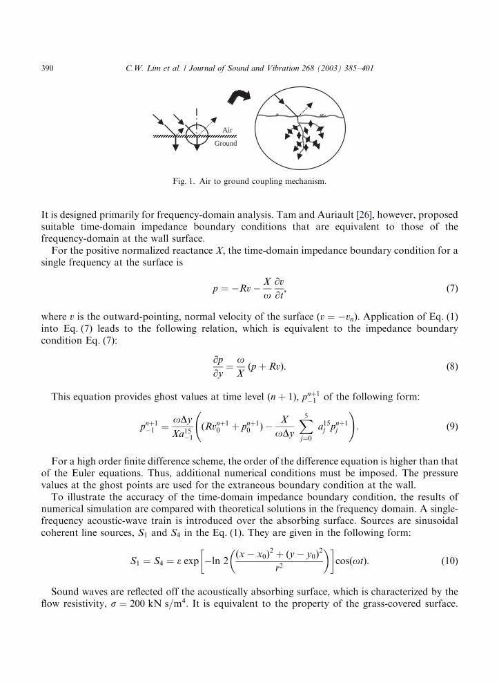
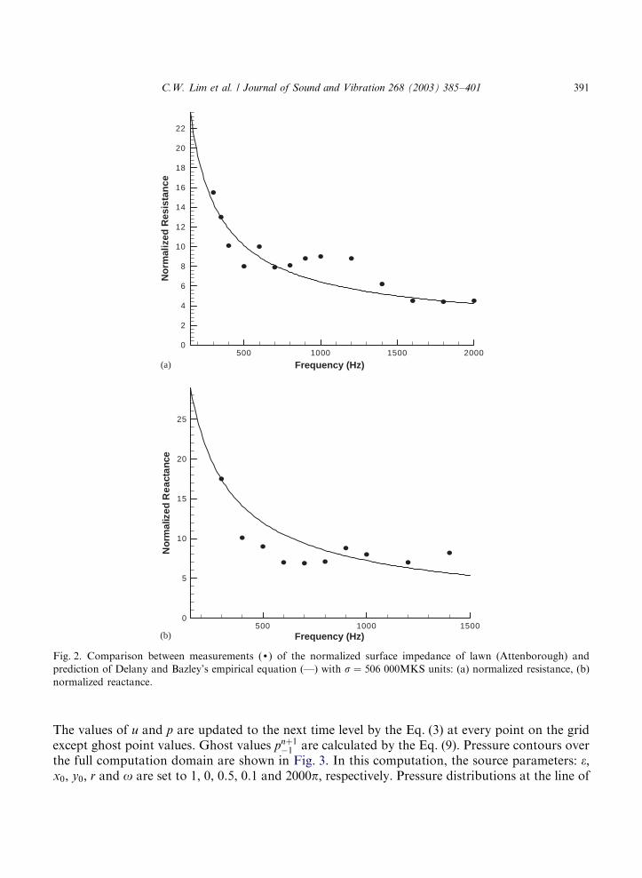
where vn is positive when pointing into the surface. The impedance is determined by a complexquantity, Z ¼ R0 þ iX 0: The use of a complex quantity is needed to account for the damping andphase shift imparted on sound waves by the acoustically treated surface. Theoreticalinvestigations [28,29] have improved the understanding of the influence of the finite impedancesurface. For example, soil is not rigid and impervious, but consists of grains of various shapes andsizes. The gaps between grains form pores that are filled with air and/or water. The sound wavesimpinging on the porous ground surface are partly reflected. Some of the sound energy penetratesinto the ground along the air-filled pores, vibrates grains and dissipates due to the viscous frictionand thermal exchanges. This mechanism is indicated in Fig. 1. In this work, the model of Delanyand Bazley [28] is used to calculate the impedance of surface. The normal surface impedancenormalized with respect to characteristic impedance of air ðr0cÞ can be expressed in terms of thedimensionless parameter, r0f =s: Here, r0 ðkg=m3Þ is the density of air, f (Hz) the frequency, ands ðN s=m4Þ the specific flow resistivity per unit thickness of the material. Delany and Bazley alsoshowed that these relations are useful for the calculation of the impedance boundary effect. TheDelany and Bazley’s empirical relation for the fibrous sound absorbing material can be expressedas follows:

Z2

r0c¼ 1þ 0:0571

r0f

s

� �0:754

þi0:0870r0f

s

� �0:732

: ð6Þ

Fig. 2 shows the comparison between the empirical model Eq. (6) of s ¼ 506 kN s=m4 and themeasurement data [29] for a lawn. There are good agreements in the normalized resistance andreactance, respectively.

2.2.2.2. Impedance wall boundary conditions. Assuming that the sound field consists of a singlefrequency o (o > 0), the pressure and velocity fields of sound waves can be expressed as pðx; tÞ ¼R e½ #pðxÞeiot� and vðx; tÞ ¼ R e½#vðxÞeiot�: The normalized impedance is defined as Z=r0c ¼ R þ iX :

ARTICLE IN PRESS


It is designed primarily for frequency-domain analysis. Tam and Auriault [26], however, proposedsuitable time-domain impedance boundary conditions that are equivalent to those of thefrequency-domain at the wall surface.

For the positive normalized reactance X, the time-domain impedance boundary condition for asingle frequency at the surface is

p ¼ �Rv �X

o@v

@t; ð7Þ

where v is the outward-pointing, normal velocity of the surface ðv ¼ �vnÞ: Application of Eq. (1)into Eq. (7) leads to the following relation, which is equivalent to the impedance boundarycondition Eq. (7):

@p

@y¼

oX

ðp þ RvÞ: ð8Þ

This equation provides ghost values at time level ðn þ 1Þ; pnþ1�1 of the following form:

pnþ1�1 ¼

oDy

Xa15�1

ðRvnþ10 þ pnþ1

0 Þ �X

oDy

X5

j¼0

a15j pnþ1

j

!: ð9Þ

For a high order finite difference scheme, the order of the difference equation is higher than thatof the Euler equations. Thus, additional numerical conditions must be imposed. The pressurevalues at the ghost points are used for the extraneous boundary condition at the wall.

To illustrate the accuracy of the time-domain impedance boundary condition, the results ofnumerical simulation are compared with theoretical solutions in the frequency domain. A single-frequency acoustic-wave train is introduced over the absorbing surface. Sources are sinusoidalcoherent line sources, S1 and S4 in the Eq. (1). They are given in the following form:

S1 ¼ S4 ¼ e exp �ln 2ðx � x0Þ

2 þ ðy � y0Þ2

r2

� � �cosðotÞ: ð10Þ

Sound waves are reflected off the acoustically absorbing surface, which is characterized by theflow resistivity, s ¼ 200 kN s=m4: It is equivalent to the property of the grass-covered surface.

ARTICLE IN PRESS

Air

Ground

Fig. 1. Air to ground coupling mechanism.


The values of u and p are updated to the next time level by the Eq. (3) at every point on the gridexcept ghost point values. Ghost values pnþ1

�1 are calculated by the Eq. (9). Pressure contours overthe full computation domain are shown in Fig. 3. In this computation, the source parameters: e;x0; y0; r and o are set to 1, 0, 0.5, 0.1 and 2000p; respectively. Pressure distributions at the line of

ARTICLE IN PRESS

(a) Frequency (Hz)

Frequency (Hz)

No

rmal

ized

Res

ista

nce

500 1000 1500 20000

2

4

6

8

10

12

14

16

18

20

22

(b)

No

rmal

ized

Rea

ctan

ce

500 1000 15000

5

10

15

20

25

Fig. 2. Comparison between measurements (d) of the normalized surface impedance of lawn (Attenborough) and

prediction of Delany and Bazley’s empirical equation (—) with s ¼ 506 000MKS units: (a) normalized resistance, (b)

normalized reactance.


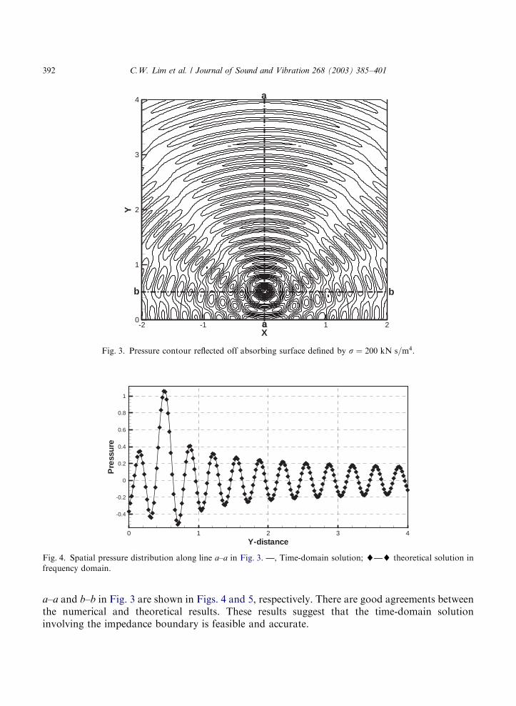
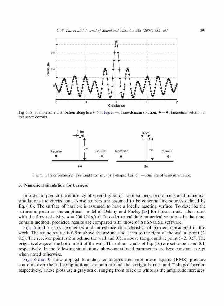
a–a and b–b in Fig. 3 are shown in Figs. 4 and 5, respectively. There are good agreements betweenthe numerical and theoretical results. These results suggest that the time-domain solutioninvolving the impedance boundary is feasible and accurate.

ARTICLE IN PRESS

X

Y

-2 -1 0 1 20

1

2

3

4

b b

a

a

Fig. 3. Pressure contour reflected off absorbing surface defined by s ¼ 200 kN s=m4:

Y-distance

Pre

ssu

re

0 1 2 3 4

-0.4

-0.2

0

0.2

0.4

0.6

0.8

1

Fig. 4. Spatial pressure distribution along line a–a in Fig. 3. —, Time-domain solution; ~—~ theoretical solution in

frequency domain.


3. Numerical simulation for barriers

In order to predict the efficiency of several types of noise barriers, two-dimensional numericalsimulations are carried out. Noise sources are assumed to be coherent line sources defined byEq. (10). The surface of barriers is assumed to have a locally reacting surface. To describe thesurface impedance, the empirical model of Delany and Bazley [28] for fibrous materials is usedwith the flow resistivity, s ¼ 200 kN s=m4: In order to validate numerical solutions in the time-domain method, predicted results are compared with those of SYSNOISE software.

Figs. 6 and 7 show geometries and impedance characteristics of barriers considered in thiswork. The sound source is 0.5m above the ground and 1.9m to the right of the wall at point (2,0.5). The receiver point is 2m behind the wall and 0.5m above the ground at point (�2, 0.5). Theorigin is always at the bottom left of the wall. The values e and r of Eq. (10) are set to be 1 and 0.1,respectively. In the following simulations, above-mentioned parameters are kept constant exceptwhen noted otherwise.

Figs. 8 and 9 show applied boundary conditions and root mean square (RMS) pressurecontours over the full computational domain around the straight barrier and T-shaped barrier,respectively. These plots use a gray scale, ranging from black to white as the amplitude increases.

ARTICLE IN PRESS

X-distance

Pre

ssur

e

-2 -1 0 1 2

0

0.4

0.8

Fig. 5. Spatial pressure distribution along line b–b in Fig. 3. —, Time-domain solution; ~—~, theoretical solution in

frequency domain.

Source Receive

0.1m

2m Source Receiver

0.5m

2m

(a) (b)

Fig. 6. Barrier geometry: (a) straight barrier, (b) T-shaped barrier. —, Surface of zero-admittance.


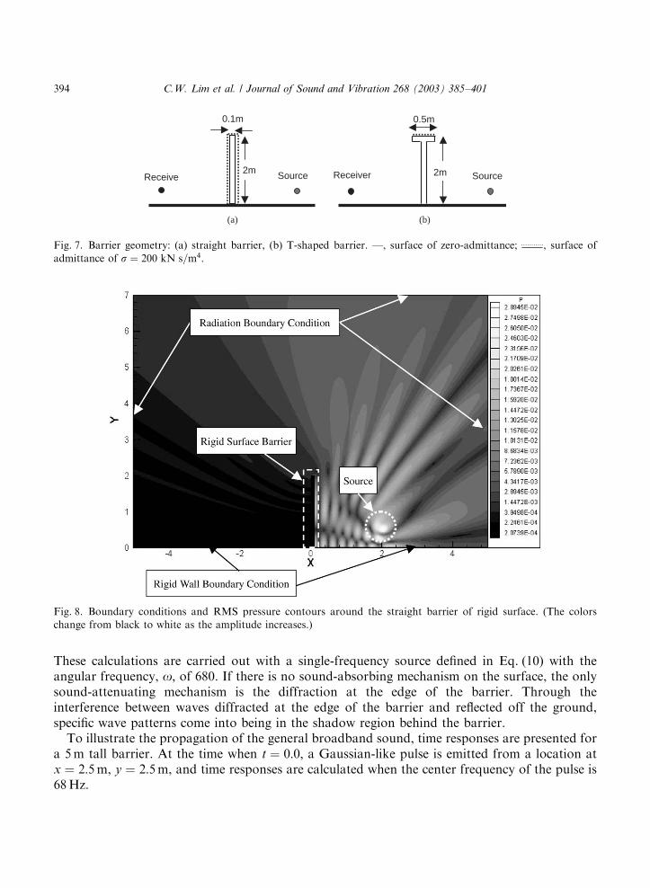
These calculations are carried out with a single-frequency source defined in Eq. (10) with theangular frequency, o; of 680. If there is no sound-absorbing mechanism on the surface, the onlysound-attenuating mechanism is the diffraction at the edge of the barrier. Through theinterference between waves diffracted at the edge of the barrier and reflected off the ground,specific wave patterns come into being in the shadow region behind the barrier.

To illustrate the propagation of the general broadband sound, time responses are presented fora 5m tall barrier. At the time when t ¼ 0:0; a Gaussian-like pulse is emitted from a location atx ¼ 2:5m, y ¼ 2:5m, and time responses are calculated when the center frequency of the pulse is68Hz.

ARTICLE IN PRESS

Source Receive

0.1m

2m Source Receiver

0.5m

2m

(a) (b)

Fig. 7. Barrier geometry: (a) straight barrier, (b) T-shaped barrier. —, surface of zero-admittance; , surface of

admittance of s ¼ 200 kN s=m4:

Fig. 8. Boundary conditions and RMS pressure contours around the straight barrier of rigid surface. (The colors

change from black to white as the amplitude increases.)


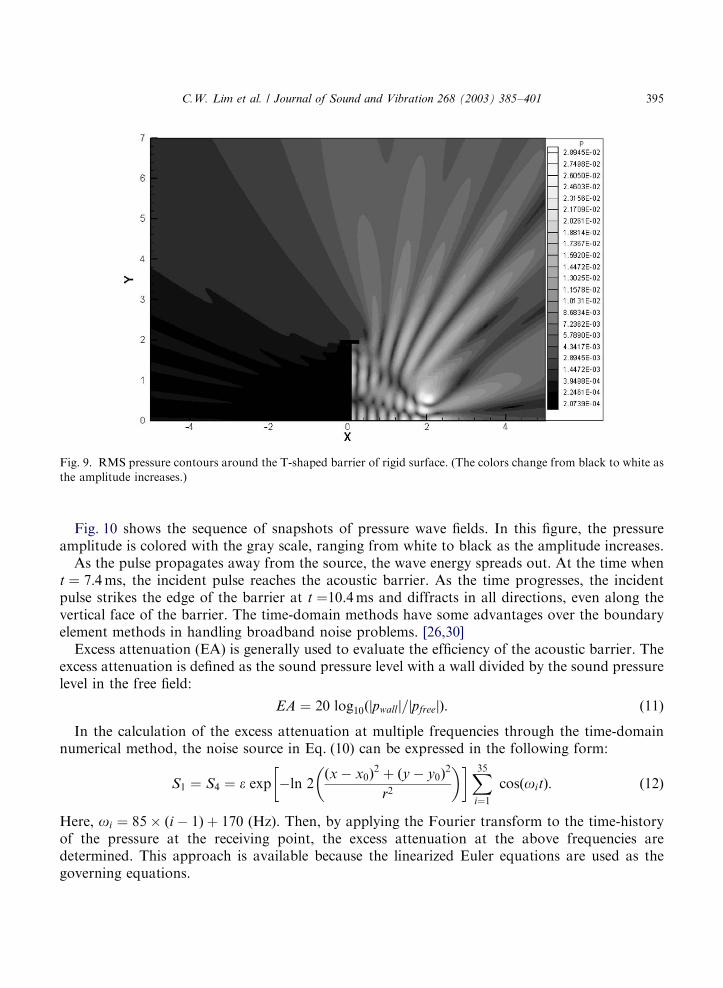
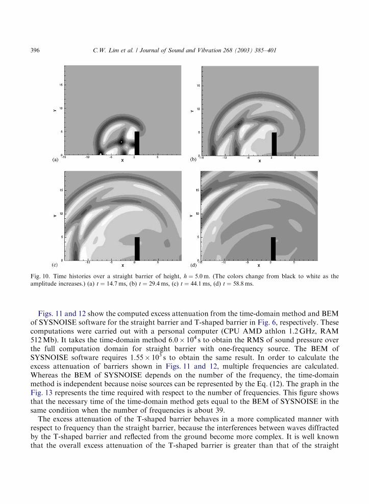
Fig. 10 shows the sequence of snapshots of pressure wave fields. In this figure, the pressureamplitude is colored with the gray scale, ranging from white to black as the amplitude increases.

As the pulse propagates away from the source, the wave energy spreads out. At the time whent ¼ 7:4ms, the incident pulse reaches the acoustic barrier. As the time progresses, the incidentpulse strikes the edge of the barrier at t ¼10.4ms and diffracts in all directions, even along thevertical face of the barrier. The time-domain methods have some advantages over the boundaryelement methods in handling broadband noise problems. [26,30]

Excess attenuation (EA) is generally used to evaluate the efficiency of the acoustic barrier. Theexcess attenuation is defined as the sound pressure level with a wall divided by the sound pressurelevel in the free field:

EA ¼ 20 log10ðjpwall j=jpfreejÞ: ð11Þ

In the calculation of the excess attenuation at multiple frequencies through the time-domainnumerical method, the noise source in Eq. (10) can be expressed in the following form:

S1 ¼ S4 ¼ e exp �ln 2ðx � x0Þ

2 þ ðy � y0Þ2

r2

� � �X35i¼1

cos oitð Þ: ð12Þ

Here, oi ¼ 85 ði � 1Þ þ 170 (Hz). Then, by applying the Fourier transform to the time-historyof the pressure at the receiving point, the excess attenuation at the above frequencies aredetermined. This approach is available because the linearized Euler equations are used as thegoverning equations.

ARTICLE IN PRESS

Fig. 9. RMS pressure contours around the T-shaped barrier of rigid surface. (The colors change from black to white as

the amplitude increases.)


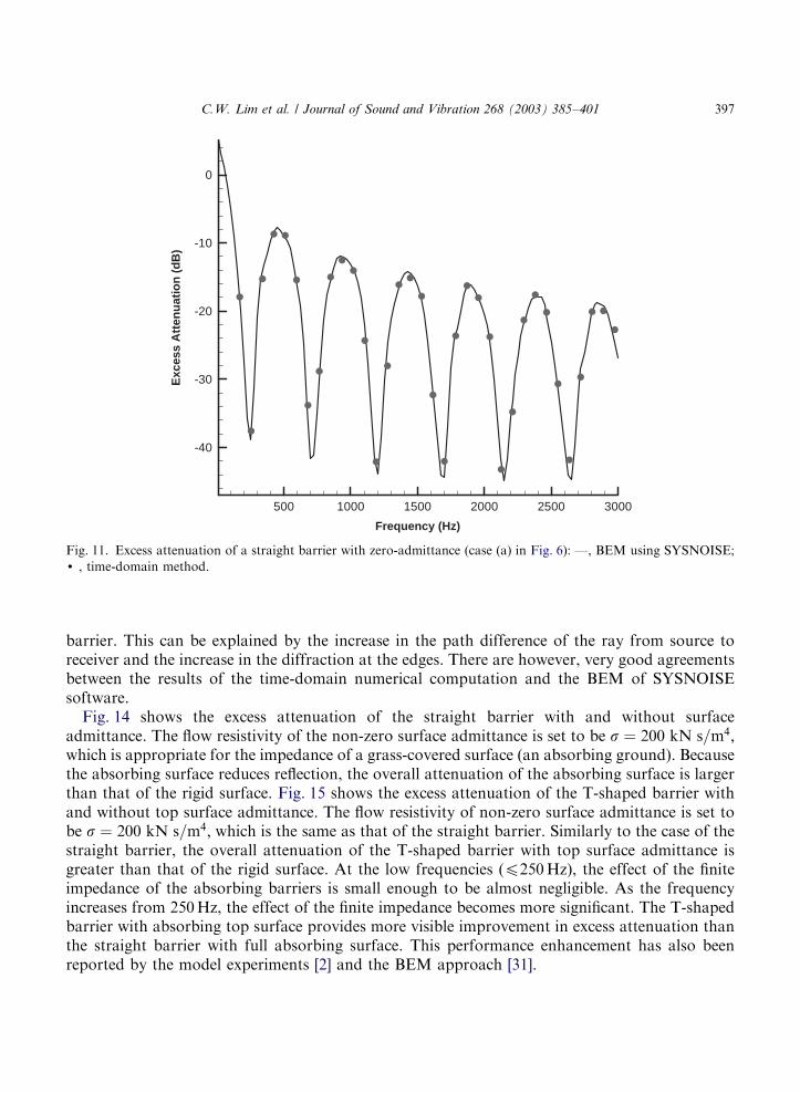
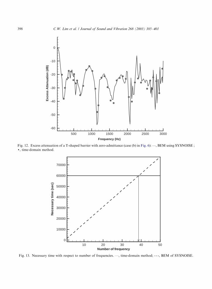
Figs. 11 and 12 show the computed excess attenuation from the time-domain method and BEMof SYSNOISE software for the straight barrier and T-shaped barrier in Fig. 6, respectively. Thesecomputations were carried out with a personal computer (CPU AMD athlon 1.2GHz, RAM512Mb). It takes the time-domain method 6.0 104 s to obtain the RMS of sound pressure overthe full computation domain for straight barrier with one-frequency source. The BEM ofSYSNOISE software requires 1.55 103 s to obtain the same result. In order to calculate theexcess attenuation of barriers shown in Figs. 11 and 12, multiple frequencies are calculated.Whereas the BEM of SYSNOISE depends on the number of the frequency, the time-domainmethod is independent because noise sources can be represented by the Eq. (12). The graph in theFig. 13 represents the time required with respect to the number of frequencies. This figure showsthat the necessary time of the time-domain method gets equal to the BEM of SYSNOISE in thesame condition when the number of frequencies is about 39.

The excess attenuation of the T-shaped barrier behaves in a more complicated manner withrespect to frequency than the straight barrier, because the interferences between waves diffractedby the T-shaped barrier and reflected from the ground become more complex. It is well knownthat the overall excess attenuation of the T-shaped barrier is greater than that of the straight

ARTICLE IN PRESS

Fig. 10. Time histories over a straight barrier of height, h ¼ 5:0 m: (The colors change from black to white as the

amplitude increases.) (a) t ¼ 14:7 ms; (b) t ¼ 29:4 ms; (c) t ¼ 44:1 ms; (d) t ¼ 58:8 ms:


barrier. This can be explained by the increase in the path difference of the ray from source toreceiver and the increase in the diffraction at the edges. There are however, very good agreementsbetween the results of the time-domain numerical computation and the BEM of SYSNOISEsoftware.

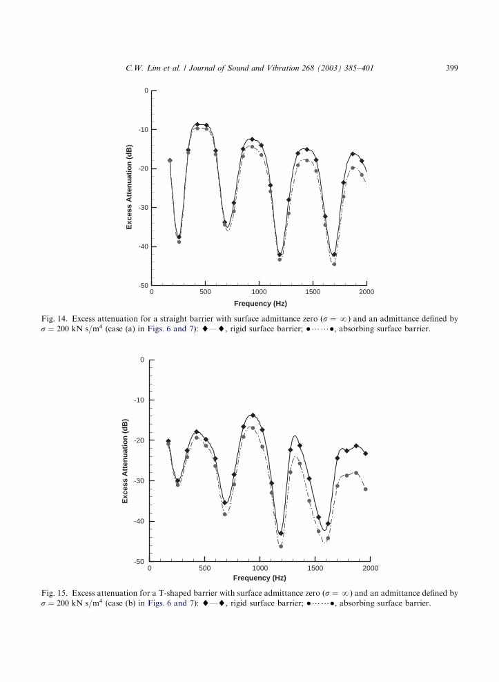
Fig. 14 shows the excess attenuation of the straight barrier with and without surfaceadmittance. The flow resistivity of the non-zero surface admittance is set to be s ¼ 200 kN s=m4;which is appropriate for the impedance of a grass-covered surface (an absorbing ground). Becausethe absorbing surface reduces reflection, the overall attenuation of the absorbing surface is largerthan that of the rigid surface. Fig. 15 shows the excess attenuation of the T-shaped barrier withand without top surface admittance. The flow resistivity of non-zero surface admittance is set tobe s ¼ 200 kN s=m4; which is the same as that of the straight barrier. Similarly to the case of thestraight barrier, the overall attenuation of the T-shaped barrier with top surface admittance isgreater than that of the rigid surface. At the low frequencies (p250Hz), the effect of the finiteimpedance of the absorbing barriers is small enough to be almost negligible. As the frequencyincreases from 250Hz, the effect of the finite impedance becomes more significant. The T-shapedbarrier with absorbing top surface provides more visible improvement in excess attenuation thanthe straight barrier with full absorbing surface. This performance enhancement has also beenreported by the model experiments [2] and the BEM approach [31].

ARTICLE IN PRESS

500 1000 1500 2000 2500 3000

-40

-30

-20

-10

0

Frequency (Hz)

Exc

ess

Att

enu

atio

n (

dB

)

Fig. 11. Excess attenuation of a straight barrier with zero-admittance (case (a) in Fig. 6): —, BEM using SYSNOISE;

d , time-domain method.


ARTICLE IN PRESS

Frequency (Hz)

Exc

ess

Att

enu

atio

n (

dB

)

500 1000 1500 2000 2500 3000

-60

-50

-40

-30

-20

-10

0

Fig. 12. Excess attenuation of a T-shaped barrier with zero-admittance (case (b) in Fig. 6): —, BEM using SYSNOISE ;

d, time-domain method.

Number of frequency

Nec

essa

ry t

ime

(sec

)

10 20 30 40 500

10000

20000

30000

40000

50000

60000

70000

Fig. 13. Necessary time with respect to number of frequencies. —, time-domain method; - - -, BEM of SYSNOISE.


ARTICLE IN PRESS

Frequency (Hz)

Exc

ess

Att

enu

atio

n (

dB

)

0 500 1000 1500 2000-50

-40

-30

-20

-10

0

Fig. 15. Excess attenuation for a T-shaped barrier with surface admittance zero ðs ¼ NÞ and an admittance defined by

s ¼ 200 kN s=m4 (case (b) in Figs. 6 and 7): ~—~, rigid surface barrier; �??�; absorbing surface barrier.

0 500 1000 1500 2000-50

-40

-30

-20

-10

0

Frequency (Hz)

Exc

ess

Att

enu

atio

n (

dB

)

Fig. 14. Excess attenuation for a straight barrier with surface admittance zero ðs ¼ NÞ and an admittance defined by

s ¼ 200 kN s=m4 (case (a) in Figs. 6 and 7): ~—~, rigid surface barrier; �??�; absorbing surface barrier.


4. Concluding remarks

A new time-domain numerical method was proposed as a powerful numerical tool to calculatethe sound propagation around the acoustic barriers with absorbing surfaces. Through thecomparison of the computational results with those of the BEM, the accuracy of the time-domainmethod was verified.

Although the main purpose of this work is to develop the time-domain method and to validateits accuracy, it is evident that the time-domain method has some advantages over boundaryelement methods. This time-domain method can handle broadband noise problems more easily.This approach can also be applied to the problems containing nonlinear noise propagationphenomena, and especially to impulsive-noise problems. Considering the merits of the time-domain numerical method, it is clear that the method offers an alternative way to solve theproblems that the boundary element methods previously found it difficult to approach.

Future work will be aimed at applying the time-domain method to the noise barrier problemscontaining high-intensity impulsive-noise sources, in which nonlinear noise propagation areimportant and broadband noise at the receiving point is concerned.

Acknowledgements

This work was sponsored by the Research Institute of Engineering Science and Brain Korea 21Project.

References

[1] W.E. Scholes, A.C. Salvidge, J.W. Sargent, Field performance of a noise barrier, Journal of Sound and Vibration

16 (1971) 627–642.

[2] D.N. May, M.M. Osman, Highway noise barriers: new shapes, Journal of Sound and Vibration 71 (1980) 73–101.

[3] Z. Maekawa, Noise reduction by screens, Applied Acoustics 1 (1968) 157–173.

[4] T. Kawai, K. Fujimoto, T. Itow, Noise propagation around a thin half plane, Acustica 38 (1978) 313–323.

[5] A.D. Pierce, Diffraction of sound around corners and over wide barriers, Journal of the Acoustical Society of

America 55 (1974) 941–955.

[6] H.G. Jonasson, Diffraction by wedges of finite acoustic impedance with applications to depressed roads, Journal

of Sound and Vibration 25 (1972) 577–585.

[7] I. Tolstoy, Exact, explicit solutions for diffraction by hard sound barriers and seamounts, Journal of the

Acoustical Society of America 85 (1989) 661–669.

[8] U.J. Kurze, G.S. Anderson, Sound attenuation by barriers, Applied Acoustics 4 (1971) 35–53.

[9] U.J. Kurze, Noise reduction by barriers, Journal of the Acoustical Society of America 55 (1974) 504–518.

[10] A. L’Esperance, The insertion loss of finite length barriers on the ground, Journal of the Acoustical Society of

America 86 (1989) 179–183.

[11] H.G. Jonasson, Sound reduction by barriers on the ground, Journal of Sound and Vibration 22 (1972) 113–126.

[12] C.I. Chessell, Propagation of noise along a finite impedance boundary, Journal of the Acoustical Society of

America 62 (1977) 825–834.

[13] T. Isei, Absorptive noise barrier on finite impedance ground, Journal of the Acoustical Society of Japan 1 (1980)

3–10.

ARTICLE IN PRESS


[14] Y.M. Lam, S.C. Roberts, A simple method for accurate prediction of finite barrier insertion loss, Journal of the

Acoustical Society of America 93 (1993) 1445–1460.

[15] P. Filippi, G. Dumery, !Etude th!eorique et num!erique de la diffraction par un !ecran mince, Acustica 21 (1969)

343–359.

[16] T. Terai, On calculation of sound fields around three-dimensional objects by integral equation methods, Journal of

Sound and Vibration 69 (1980) 71–100.

[17] R. Seznec, Diffraction of sound around barriers: use of the boundary elements technique, Journal of Sound and

Vibration 73 (1980) 195–209.

[18] D.C. Hothersall, S.N. Chandler-Wilde, M.N. Hajmirzae, Efficiency of single noise barriers, Journal of Sound and

Vibration 146 (1991) 303–322.

[19] D. Duhamel, P. Sergent, Sound propagation over noise barriers with absorbing ground, Journal of Sound and

Vibration 218 (1998) 799–823.

[20] P.A. Morgan, D.C. Hothersall, S.N. Chandler-Wilde, Influence of shape and absorbing surface—a numerical

study of railway barriers, Journal of Sound and Vibration 217 (1998) 405–417.

[21] P. Jean, J. Defrance, Y. Gabillet, The importance of source type on the assessment of noise barriers, Journal of

Sound and Vibration 226 (1999) 201–216.

[22] C.K. Tam, Computational aeroacoustics: issues and methods, American Institute of Aeronautics and Astronautics

Journal 33 (1995) 1788–1796.

[23] V.L. Wells, R.A. Renaut, Computing aerodynamically generated noise, Fluid Mechanics 29 (1997) 161–199.

[24] S.K. Lele, Compact finite difference schemes with spectral-like resolution, Journal of Computational Physics 103

(1992) 16–42.

[25] C.K.W. Tam, J.C. Webb, Dispersion-relation-preserving finite difference schemes for computational acoustics,

Journal of Computational Physics 107 (1997) 262–281.

[26] C.K.W. Tam, L. Auriault, Time-domain impedance boundary conditions for computational aeroacoustics,

American Institute of Aeronautics and Astronautics Journal 34 (1996) 917–923.

[27] C.K.W. Tam, J.C. Webb, Z. Dong, A study of the short wave components in computational acoustics, Journal of

Computational Acoustics 1 (1993) 1–30.

[28] M.E. Delany, E.N. Bazley, Acoustical properties of fibrous absorbent materials, Applied Acoustics 3 (1976)

105–116.

[29] K. Attenborough, Acoustical impedance models for outdoor ground surfaces, Journal of Sound and Vibration 99

(1985) 521–544.

[30] Y. Ozyoruk, L.N. Long, M.G. Jones, Time-domain numerical simulation of a flow-impedance tube, Journal of

Computational Physics 146 (1998) 29–57.

[31] K. Fujiwara, D.C. Hothersall, C.H. Kim, Noise barriers with reactive surfaces, Applied Acoustics 53 (1997)

255–272.

ARTICLE IN PRESS


Documents

Time-domain numerical computation of noise reduction …aancl.snu.ac.kr/aancl/research/International Journal/[2003... · Time-domain numerical computation of noise reduction by