Embed Size (px)
Citation preview
JOURNAL OF THE MECHANICS AND PHYSICS OF SOLIDS, IN PRESS.
TIME-HARMONIC GREEN’S FUNCTION
AND BOUNDARY INTEGRAL FORMULATION FOR
INCREMENTAL NONLINEAR ELASTICITY:
DYNAMICS OF WAVE PATTERNS AND SHEAR BANDS
Davide Bigoni(1) Domenico Capuani(2)
(1)Dipartimento di Ingegneria Meccanica e Strutturale, Università di Trento, Via Mesiano 77 – 38050 Povo, Trento, Italia. Email [email protected].
(2) Dipartimento di Architettura, Università di Ferrara,
Via Quartieri 8– 44100 Ferrara, Italia. Email [email protected]
Abstract. Superimposed dynamic, time-harmonic incremental deformations are considered in an elastic, orthotropic and incompressible, infinite body, subject to plane, homogeneous –but otherwise arbitrary− deformation. The dynamic, infinite body Green’s function is found and, in addition, new boundary integral equations are obtained for incremental in-plane hydrostatic stress and displacements. These findings open the way to integral methods in incremental, dynamic elasticity. Moreover, the Green’s function is employed as a dynamic perturbation to analyse interaction between wave propagation and shear band formation. Depending on anisotropy and pre-stress level, peculiar wave patterns emerge with focussing and shadowing effects of signals, which may remain undetected by the usual criteria based on analysis of weak discontinuity surfaces.
Key words: Dynamic Green’s function, boundary integral equations, nonlinear elasticity,
shear bands, boundary element method, wave propagation, pre-stressed media, anisotropy.
1. Introduction
FINDINGS by Bigoni and Capuani (2002) pertaining to quasi-static deformation of pre-
stressed, elastic orthotropic and incompressible materials are extended in the present article to
the dynamic, time-harmonic regime. In particular, infinite-body, dynamic Green’s functions
and boundary integral equations for incremental displacements and in-plane incremental
hydrostatic stress, are obtained for small −isochoric and two-dimensional− deformation
superimposed upon a given nonlinear elastic and homogeneous strain. Due to the hypothesis
of time-harmonic deformation, the regime classification of the governing differential
equations remains identical to the quasi-static case, so that all obtained solutions lie within the
elliptic range. A perturbation in terms of a pulsating dipole can be therefore obtained and
1
JOURNAL OF THE MECHANICS AND PHYSICS OF SOLIDS, IN PRESS.
employed to analyse material instabilities arising near the boundary of ellipticity loss. The
perturbative approach is general −since it can be employed for any incrementally linear
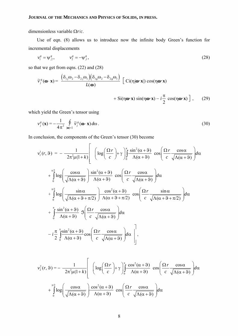
constitutive equation, dynamic loadings and inhomogeneous material (Willis, 1991)− and is
capable of revealing aspects which may remain undetected using methods for material
instabilities based on weak discontinuity surfaces (loss of ellipticity, e.g. Knowles and
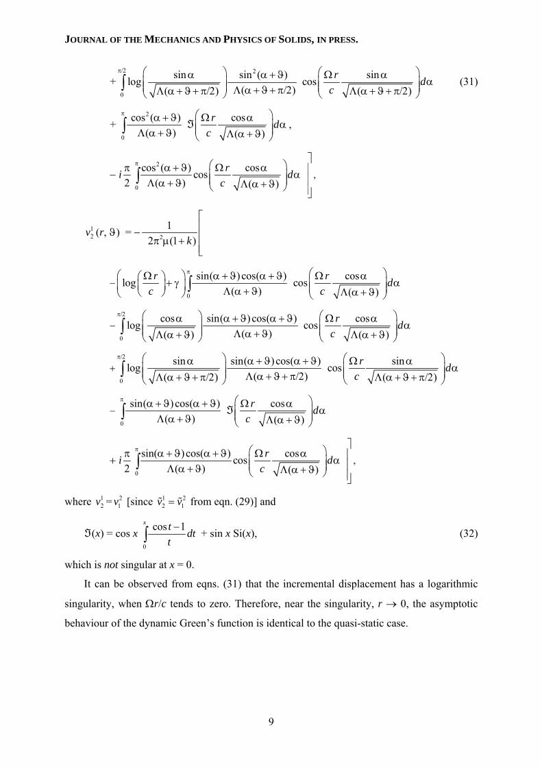
Sternberg, 1978). For instance, the perturbative approach has revealed shear band formation
for a Mooney-Rivlin material in the quasi-static case (Bigoni and Capuani, 2002, their Fig. 3),
a circumstance confirmed by the present dynamic analysis, but not detected by the
conventional approach.
Results presented in this article provide a basis for the analysis of propagation of
dynamic disturbances near the boundary of loss of ellipticity. Depending on the level of pre-
stress and anisotropy, wave patterns are shown to emerge, with focussing of signals in the
direction of shear bands. Varying the direction of the dynamic perturbation excites different
wave patterns, which tend to degenerate to families of plane waves parallel to the shear bands,
when the elliptic boundary is approached.
Another possibility related to the finding of a Green’s function is the formulation of a
boundary element technique for the solution of incremental boundary value problems. For
quasi-static deformation, this technique was proved to possess certain advantages −related for
instance to the treatment of the incompressibility constraint− with respect to other numerical
techniques, such as finite element methods (Brun et al. 2003 a, b). Now the development of
the technique in dynamics requires the finding of new boundary integral equations. While the
integral equation for incremental displacements does not formally change with respect to the
quasi-static case, a generalization is given of the integral representation for incremental in-
plane hydrostatic stress obtained by Bigoni and Capuani (2002).
The paper is organized as follows. After a brief presentation of the constitutive
framework (Section 2), the dynamic Green’s function set, composed of incremental
displacements, eqn. (31), and in-plane incremental hydrostatic stress, eqn. (40), is obtained in
Section 3. Wave patterns produced by a dynamic perturbation at different pre-stress levels are
analyzed in Section 4 and, finally, boundary integral equations for incremental displacement,
eqn. (43), and in-plane incremental hydrostatic stress, eqn. (54), are given in Section 5.
2
JOURNAL OF THE MECHANICS AND PHYSICS OF SOLIDS, IN PRESS.
2. Constitutive framework
We refer to the two-dimensional Biot (1965) constitutive framework detailed in Bigoni and
Capuani (2002) and Brun et al. (2003a). In the principal reference system of Cauchy stress
(here denoted by in-plane indices 1 and 2) and using a Lagrangean formulation of the field
equations with the current state taken as reference, the constitutive relation can be written as
= ijt& ijklvl,k + p& δij , (1)
where1ijt& is the increment of nominal stress tij, induced by the gradient of incremental
displacement vi through the fourth-order tensor ijkl and, independently, by the in-plane
hydrostatic stress increment p& . Note that tensor ijkl possesses the major symmetry ijkl =
klij and is a function of the principal components of Cauchy stress σ1 and σ2, describing the
pre-stress, and of two incremental moduli µ and *µ (which can depend arbitrarily on the
current stress and strain). It is defined by the following non-null components
1111 = −*µ2σ
− p, 1122 = 2211 = − *µ , 2222 = *µ +2σ
− p,
1212 = µ +2σ , 1221 = 2112 = µ − p, 2121 = µ −
2σ , (2)
with
σ = σ1 − σ2, 221 σ+σ
=p . (3)
The constitutive equations (1) are complemented by the incompressibility constraint
vi,i = 0. (4)
Constitutive equations (1)-(4) describe a broad class of material behaviours, including all
possible elastic incompressible material isotropic in an initial state (Biot, 1965; Brun et al.
2003a), but also materials which are orthotropic with respect to the current principal stress
directions (1 and 2). The latter situation has interesting practical applications in the field of
fiber-reinforced elastic materials. Here, loss of ellipticity may explain occurrence of different
1 The standard, indicial notation employed by Bigoni and Capuani (2002) is used throughout this paper, where a comma denotes partial differentiation, repeated indices are summed (between 1 and 2) and δij is the Kronecker
3
JOURNAL OF THE MECHANICS AND PHYSICS OF SOLIDS, IN PRESS.
failure modes, such as fiber kinking, splitting and debonding (Merodio and Pence, 2001;
Merodio and Ogden, 2002). In particular, the constitutive framework given by Merodio and
Pence (2001) and Merodio and Ogden (2002) can be given the format employed in the present
paper when the principal components of current stress are aligned normal and parallel to the
fibers. In the following, no specific assumptions will be made on the dependence of and µ
on the current state.
*µ
3. The dynamic Green’s function set
Superimposed incremental deformations upon a homogeneously pre-deformed infinite
medium are considered, produced by application of a time-harmonic point load acting at the
point x = 0 and with components 1f& (t), 2f& (t) at time t, along the principal stress axes. While
the current state of stress trivially satisfies equilibrium, the equations of motion for
superimposed disturbances are
,ij it& + = ρ , (5) ( )jf δ x&,j ttv
where δ is the two-dimensional Dirac delta function and ,t denotes the material time
derivative. In the hypothesis of time-harmonic motion with circular frequency Ω, every field
g(x, t) can be expressed as g(x) e−iΩt and eqns. (5) become
(2 *µ − µ)v1,11 + (µ −2σ )v1,22 + 1f& δ(x) = − ,1π& − ρ Ω2 v1,
(2 *µ − µ)v2,22 + (µ +2σ )v2,11 + 2f& δ(x) = − ,2π& − ρ Ω2 v2, (6)
where
π& = 11 22
2t t+& &
= p& − 1,12vσ (7)
is the increment of in-plane nominal hydrostatic stress. Note that, due to the time-harmonic
assumption, eqns. (6) are independent of time.
Introducing the stream function ψ(x1, x2) as
v1 = ψ,2 , v2 = − ψ,1, (8)
and the dimensionless pre-stress parameter
delta. Superposed dot denotes an incremental quantity.
4
JOURNAL OF THE MECHANICS AND PHYSICS OF SOLIDS, IN PRESS.
k = µ
σ2
, (9)
eqns. (6)1 and (6)2 can be combined to give
(1 + k) ψ,1111 + 2(2 ∗µµ
− 1) ψ,1122 + (1 − k) ψ,2222 + 1fµ
&δ,2 − 2f
µ
&δ,1
= − 2ρΩ
µ (ψ,11+ψ,22). (10)
It is important to realize now that, since only the principal part of a differential operator plays
a role in determining the regime classification (see for instance Renardy and Rogers, 1993),
the classification of equation (10) remains the same as for the quasi-static case.
Since the classification of governing differential equations does not change from the
quasi-static case, we remark that all results in this paper will be restricted to the elliptic
regime, defined through the condition that scalars γ1 and γ2
k+
∆±µµ
−=
⎭⎬⎫
γγ
1
21 *
2
1 , 2
**2 44 ⎟⎟⎠
⎞⎜⎜⎝
⎛µµ
+µµ
−=∆ k , (11)
are either both real and negative in the elliptic imaginary regime (EI) or a conjugate pair in
the elliptic complex regime (EC). Note that ∆ is positive in (EI) and negative in (EC).
A consequence of the above discussion is that the emergence of weakly discontinuous
surfaces corresponds in the present context to failure of ellipticity, as in the quasi-static case.
This occurs in a continuous loading path (starting from E) either when k = 1 (so that γ1 = 0) or
when ∆ = 0 (so that γ1 = γ2). The former case defines the elliptic-imaginary/parabolic
boundary, while the latter the elliptic-complex/hyperbolic boundary.
3.1 The dynamic Green’s function for incremental displacements
Taking if& = δig , eqn. (10) can be rewritten as
µ L ψg + (δ1g 2x∂⋅∂
− δ2g 1x∂⋅∂ ) δ(x) = − ρ Ω2 ∇2 ψg, (12)
where ∇2 is the Laplacian and L is the linear differential operator defined as
5
JOURNAL OF THE MECHANICS AND PHYSICS OF SOLIDS, IN PRESS.
L (⋅) = (1 + k) 41
4
x∂⋅∂ + 2(2 ∗µ
µ− 1) 2
221
4
xx ∂∂⋅∂ + (1 − k) 4
2
4
x∂⋅∂ . (13)
We follow here the procedure used by Bigoni and Capuani (2002) of employing plane wave
expansions of the functions involved (Gel’fand and Shilov, 1964; see Willis, 1973, for
applications in elasticity). In particular, the plane wave expansions of the δ function and of
the stream function ψg(x) are
δ(x) = − 241π 1| =ω|
2)( x⋅ω
ωd , ψg(x) = − 24
1π 1| =ω|
ω⋅ψ dg )(~ xω , (14)
where ω is a unit vector. Substituting representations (14) into eqn. (12) yields
( )g ′′′′ψ% +)(
ΩρωL
2
( )g ′′ψ% = 2 1 2 2 13( ) ( )
g g
Lδ ω − δ ω
⋅xω ω, (15)
where a prime denotes differentiation with respect to the variable ω⋅x and
L(ω) = 42ωµ ⎥
⎦
⎤⎢⎣
⎡γ−
ωω
⎥⎦
⎤⎢⎣
⎡γ−
ωω
+ 222
21
122
21)1( k > 0. (16)
Note that the velocity of a transverse plane wave propagating in the direction defined by the
unit vector ω is [L(ω)/ρ]1/2.
The integral of differential equation (15) with respect to the variable ω⋅x can be obtained
through variation of parameters in the form
gψ~ (ω⋅x) = ( )1 2 2 1g g
L
δ ω − δ ω
Ω ρ ( )ω Ci(η|ω⋅x|) sin(ηω⋅x) − Si(ηω⋅x) cos(ηω⋅x)
+ A1 sin(ηω⋅x) + A2 cos(ηω⋅x) + i[A3 sin(ηω⋅x) + A4 cos(ηω⋅x)], (17)
where Aj (j=1,..,4) are arbitrary constants, i = 1− , η is the wave-number (in the direction ω)
η = L
ρΩ
( )ω, (18)
and Ci and Si are the cosine integral and sine integral functions defined as
Si(x) = 0
sinx t dtt∫ , Ci(x) = γ + log x +
0
cos 1x t dtt
−∫ , (19)
where γ ≅ 0.577216 is the Euler Gamma constant.
To determine now constants Aj in eqn. (17), let us consider the far-field approximation in
6
JOURNAL OF THE MECHANICS AND PHYSICS OF SOLIDS, IN PRESS.
the variable ω⋅x of the following term
Ci(ηω⋅x) sin(ηω⋅x) − Si(ηω⋅x) cos(ηω⋅x) = − 2π cos(ηω⋅x) + O ⎟
⎠⎞
⎜⎝⎛
• xω1 , (ω⋅x → +∞). (20)
Neglecting an arbitrary harmonic solution, from eqns. (17) and (20) we get the far-field
approximation for gψ~
gψ~ (ω⋅x) = − ( )1 2 2 1g g
L2
δ ω − δ ω
ρΩ ( )ω [
2π cos(ηω⋅x) + i
2π sin(ηω⋅x)] + O ⎟
⎠⎞
⎜⎝⎛
• xω1 , (21)
which features only outgoing waves.
As a consequence of asymptotic representation (21), constants Aj remain determinate and eqn.
(17) becomes
gψ~ (ω⋅x) = ( )1 2 2 1g g
L2
δ ω − δ ω
ρΩ ( )ω [Ci(η|ω⋅x|) sin(ηω⋅x)
− Si(ηω⋅x) cos(ηω⋅x) − i2π sin(ηω⋅x)]. (22)
Introducing the polar coordinates r = |x| and ϑ of the generic point, a substitution of eqn. (22)
into the plane wave expansion (14)2 provides the stream function
ψ g (r, ϑ) = − 1c22π ρΩ 0
sin( ) cos( ) ( )
g r dc
π ⎛ ⎞α + ϑ + (1− )π/2 Ω αΞ α⎜ ⎟⎜ ⎟Λ α + ϑ Λ α + ϑ⎝ ⎠
∫ , (23)
where
Ξ(x) = sin x Ci(|x|) − cos x Si(x) − i2π sin x . (24)
Consistently with eqn. (16), the function Λ in eqn. (23) is defined as
Λ(α) = sin4α [cot2α – γ1] [cot2α – γ2] > 0, (25)
and
c = ρ+µ )1( k (26)
is the propagation speed of a transverse wave travelling parallel to x1-axis whereas
c ( )Λ α (27)
is the velocity of propagation in the direction singled out by angle α.
Note that the stream function (23) is not singular at r = 0 and it depends on ϑ and the
7
JOURNAL OF THE MECHANICS AND PHYSICS OF SOLIDS, IN PRESS.
dimensionless variable Ωr/c.
Use of eqn. (8) allows us to introduce now the infinite body Green’s function for
incremental displacements
1 ,2g gv = ψ , 2 ,1
g gv = −ψ , (28)
so that we get from eqns. (22) and (28)
)(~ x⋅ωgjv =
( )( )1 2 2 1 1 2 2 1j j g g
Lδ ω − δ ω δ ω − δ ω
( )ω[Ci(η|ω⋅x|) cos(ηω⋅x)
+ Si(ηω⋅x) sin(ηω⋅x) − i2π cos(ηω⋅x)], (29)
which yield the Green’s tensor using
gjv (x) = − 24
1π 1| =ω|
ω⋅ dv gj )(~ xω . (30)
In conclusion, the components of the Green’s tensor (30) become
11v (r, ϑ) = −
12 (1 )k2
⎡⎢⎢π µ +⎢⎣
2
0
sin ( ) coslog cos( ) ( )
r r dc c
π ⎛ ⎞⎛ ⎞Ω α + ϑ Ω α⎛ ⎞ + γ α⎜ ⎟⎜ ⎟⎜ ⎟ ⎜ ⎟Λ α + ϑ Λ α + ϑ⎝ ⎠⎝ ⎠ ⎝ ⎠∫
+2
0
cos sin ( ) coslog cos( )( ) ( )
r dc
π/2 ⎛ ⎞ ⎛α α + ϑ Ω α ⎞α⎜ ⎟ ⎜⎜ ⎟ ⎜Λ α + ϑΛ α + ϑ Λ α + ϑ⎝ ⎠ ⎝
∫ ⎟⎟⎠
+2
0
sin cos ( ) sinlog cos( )( ) ( )
r dc
π/2 ⎛ ⎞ ⎛α α + ϑ Ω αα⎜ ⎟ ⎜⎜ ⎟ ⎜Λ α + ϑ + π/2Λ α + ϑ + π/2 Λ α + ϑ + π/2⎝ ⎠ ⎝
∫⎞⎟⎟⎠
+ 2
0
sin ( ) cos( ) ( )
r dc
π ⎛ ⎞α + ϑ Ω αα⎜ ⎟⎜ ⎟Λ α + ϑ Λ α + ϑ⎝ ⎠
∫
− i2π 2
0
sin ( ) coscos( ) ( )
r dc
π ⎤⎛ ⎞α + ϑ Ω α ⎥α⎜ ⎟ ⎥⎜Λ α + ϑ Λ α + ϑ⎝ ⎠⎟
⎥⎦∫ ,
22v (r, ϑ) = −
12 (1 )k2
⎡⎢⎢π µ +⎢⎣
2
0
cos ( ) coslog cos( ) ( )
r r dc c
π ⎛ ⎞⎛ ⎞Ω α + ϑ Ω α⎛ ⎞ + γ α⎜ ⎟⎜ ⎟⎜ ⎟ ⎜ ⎟Λ α + ϑ Λ α + ϑ⎝ ⎠⎝ ⎠ ⎝ ⎠∫
+2
0
cos cos ( ) coslog cos( )( ) ( )
r dc
π/2 ⎛ ⎞ ⎛α α + ϑ Ω α ⎞α⎜ ⎟ ⎜⎜ ⎟ ⎜Λ α + ϑΛ α + ϑ Λ α + ϑ⎝ ⎠ ⎝
∫ ⎟⎟⎠
8
JOURNAL OF THE MECHANICS AND PHYSICS OF SOLIDS, IN PRESS.
+2
0
sin sin ( ) sinlog cos( )( ) ( )
r dc
π/2 ⎛ ⎞ ⎛α α + ϑ Ω αα⎜ ⎟ ⎜⎜ ⎟ ⎜Λ α + ϑ + π/2Λ α + ϑ + π/2 Λ α + ϑ + π/2⎝ ⎠ ⎝
∫⎞⎟⎟⎠
(31)
+ 2
0
cos ( ) cos( ) ( )
r dc
π ⎛ ⎞α + ϑ Ω αα⎜⎜Λ α + ϑ Λ α + ϑ⎝ ⎠
∫ ⎟⎟ ,
− i2π 2
0
cos ( ) coscos( ) ( )
r dc
π ⎤⎛ ⎞α + ϑ Ω α ⎥α⎜ ⎟ ⎥⎜Λ α + ϑ Λ α + ϑ⎝ ⎠⎟
⎥⎦∫ ,
12v (r, ϑ) = − 1
2 (1 )k2
⎡⎢⎢π µ +⎢⎣
−0
sin( )cos( ) coslog cos( ) ( )
r r dc c
π ⎛ ⎞⎛ ⎞Ω α + ϑ α + ϑ Ω α⎛ ⎞ + γ α⎜ ⎟⎜ ⎟⎜ ⎟ ⎜ ⎟Λ α + ϑ Λ α + ϑ⎝ ⎠⎝ ⎠ ⎝ ⎠∫
−0
cos sin( )cos( ) coslog cos( )( ) ( )
r dc
π/2 ⎛ ⎞ ⎛α α + ϑ α + ϑ Ω αα⎜ ⎟ ⎜⎜ ⎟ ⎜Λ α + ϑΛ α + ϑ Λ α + ϑ⎝ ⎠ ⎝
∫⎞⎟⎟⎠
+0
sin sin( )cos( ) sinlog cos( )( ) ( )
r dc
π/2 ⎛ ⎞ ⎛α α + ϑ α + ϑ Ω α ⎞α⎜ ⎟ ⎜⎜ ⎟ ⎜Λ α + ϑ + π/2Λ α + ϑ+ π/2 Λ α + ϑ + π/2⎝ ⎠ ⎝
∫ ⎟⎟⎠
− 0
sin( )cos( ) cos( ) ( )
r dc
π ⎛ ⎞α + ϑ α + ϑ Ω αα⎜ ⎟⎜ ⎟Λ α + ϑ Λ α + ϑ⎝ ⎠
∫
+ i2π
0
sin( )cos( ) coscos( ) ( )
r dc
π ⎤⎛ ⎞α + ϑ α + ϑ Ω α ⎥α⎜ ⎟ ⎥⎜Λ α + ϑ Λ α + ϑ⎝ ⎠⎟
⎥⎦∫ ,
where = [since from eqn. (29)] and 12v 2
1v 12v v=% %2
1
(x) = cos x 0
cos 1x t dtt
−∫ + sin x Si(x), (32)
which is not singular at x = 0.
It can be observed from eqns. (31) that the incremental displacement has a logarithmic
singularity, when Ωr/c tends to zero. Therefore, near the singularity, r → 0, the asymptotic
behaviour of the dynamic Green’s function is identical to the quasi-static case.
9
JOURNAL OF THE MECHANICS AND PHYSICS OF SOLIDS, IN PRESS.
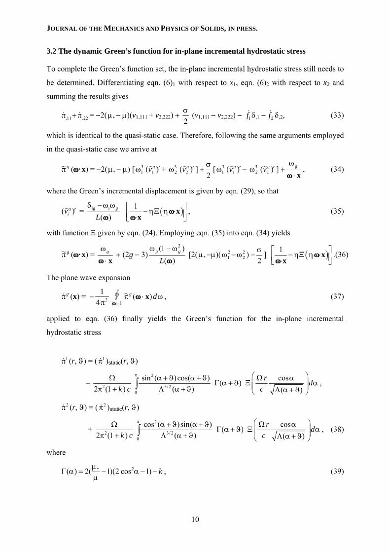
3.2 The dynamic Green’s function for in-plane incremental hydrostatic stress
To complete the Green’s function set, the in-plane incremental hydrostatic stress still needs to
be determined. Differentiating eqn. (6)1 with respect to x1, eqn. (6)2 with respect to x2 and
summing the results gives
,11π& + = −2( − µ)(v,22π& *µ 1,111 + v2,222) + 2σ (v1,111 − v2,222) − 1f& δ,1 − 2f& δ,2, (33)
which is identical to the quasi-static case. Therefore, following the same arguments employed
in the quasi-static case we arrive at
gπ~ (ω⋅x) = −2( − µ) [*µ 31ω 1( )gv ′% + 3
2ω 2( )gv ′% ] +2σ [ 3
1ω 1( )gv ′% − 32ω 2( )gv ′% ] +
x⋅
ω
ωg , (34)
where the Green’s incremental displacement is given by eqn. (29), so that
( )giv ′% =
( )ig i g
Lδ − ω ω
ω(1⎡ ⎤− ηΞ η ⋅⎢ ⎥⋅⎣ ⎦
xx
ωω
) , (35)
with function Ξ given by eqn. (24). Employing eqn. (35) into eqn. (34) yields
gπ~ (ω⋅x) = x⋅
ω
ωg + (2g − 3)
)()2
ωLgg ω−(1ω
[2( *µ −µ)( ) −21ω − 2
2ω2σ ] (1 )⎡ ⎤− ηΞ η ⋅⎢ ⎥⋅⎣ ⎦
xx
ωω
.(36)
The plane wave expansion
gπ& (x) = − 241π 1| =ω|
ω⋅π dg )(~ xω , (37)
applied to eqn. (36) finally yields the Green’s function for the in-plane incremental
hydrostatic stress
1π& (r, ϑ) = ( )1π& static(r, ϑ)
− k c2
Ω2π (1+ )
2
3/ 20
sin ( )cos( ) cos( )( ) ( )
r dc
π ⎛ ⎞α + ϑ α + ϑ Ω αΓ α + ϑ Ξ α⎜ ⎟⎜ ⎟Λ α + ϑ Λ α + ϑ⎝ ⎠
∫ ,
2π& (r, ϑ) = ( )2π& static(r, ϑ)
+ k c2
Ω2π (1+ )
2
3/ 20
cos ( )sin( ) cos( )( ) ( )
r dc
π ⎛ ⎞α + ϑ α + ϑ Ω αΓ α + ϑ Ξ α⎜ ⎟⎜ ⎟Λ α + ϑ Λ α + ϑ⎝ ⎠
∫ , (38)
where
k−−α−µµ
=αΓ )1cos2)(1(2)( 2* , (39)
10
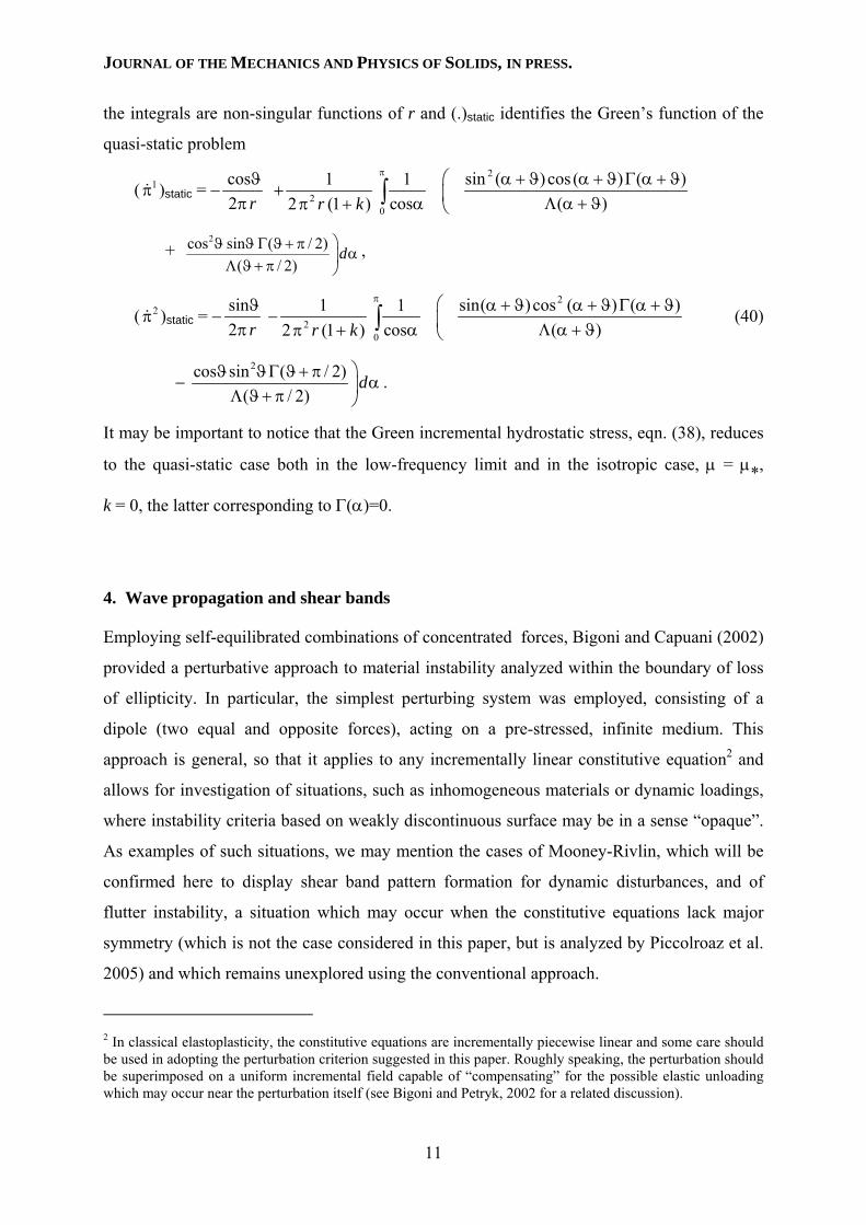
JOURNAL OF THE MECHANICS AND PHYSICS OF SOLIDS, IN PRESS.
the integrals are non-singular functions of r and (.)static identifies the Green’s function of the
quasi-static problem
( )1π& static = −rπϑ
2cos +
)1(21
2 kr +π 0
1cos
π ⎛⎜α ⎝
∫ )()()(cos)(sin 2
ϑ+αΛϑ+αΓϑ+αϑ+α
+ 2cos sin ( / 2)
( / 2)d
⎞ϑ ϑ Γ ϑ + πα⎟Λ ϑ + π ⎠
,
( )2π& static = −rπϑ
2sin −
)1(21
2 kr +π 0
1cos
π ⎛⎜α ⎝
∫ )()()(cos)(sin 2
ϑ+αΛϑ+αΓϑ+αϑ+α (40)
− 2cos sin ( / 2)
( / 2)d
⎞ϑ ϑΓ ϑ + πα⎟Λ ϑ + π ⎠
.
It may be important to notice that the Green incremental hydrostatic stress, eqn. (38), reduces
to the quasi-static case both in the low-frequency limit and in the isotropic case, µ = µ*,
k = 0, the latter corresponding to Γ(α)=0.
4. Wave propagation and shear bands
Employing self-equilibrated combinations of concentrated forces, Bigoni and Capuani (2002)
provided a perturbative approach to material instability analyzed within the boundary of loss
of ellipticity. In particular, the simplest perturbing system was employed, consisting of a
dipole (two equal and opposite forces), acting on a pre-stressed, infinite medium. This
approach is general, so that it applies to any incrementally linear constitutive equation2 and
allows for investigation of situations, such as inhomogeneous materials or dynamic loadings,
where instability criteria based on weakly discontinuous surface may be in a sense “opaque”.
As examples of such situations, we may mention the cases of Mooney-Rivlin, which will be
confirmed here to display shear band pattern formation for dynamic disturbances, and of
flutter instability, a situation which may occur when the constitutive equations lack major
symmetry (which is not the case considered in this paper, but is analyzed by Piccolroaz et al.
2005) and which remains unexplored using the conventional approach.
2 In classical elastoplasticity, the constitutive equations are incrementally piecewise linear and some care should be used in adopting the perturbation criterion suggested in this paper. Roughly speaking, the perturbation should be superimposed on a uniform incremental field capable of “compensating” for the possible elastic unloading which may occur near the perturbation itself (see Bigoni and Petryk, 2002 for a related discussion).
11
JOURNAL OF THE MECHANICS AND PHYSICS OF SOLIDS, IN PRESS.
Similarly to the quasi-static case, a time-harmonic pulsating dipole is used as a perturbing
agent, acting on a pre-stressed infinite medium. The effect of the dynamic perturbation decays
with distance, but the decay becomes slower and slower in a path (in the k vs. µ*/µ space)
towards the boundary of ellipticity. The interesting feature is represented by the deformation
patterns emerging when the loss of ellipticity is approached.
We begin with the simple example of a Mooney-Rivlin material (in our case of plane
strain deformation this material model coincides with a neo-Hookean material) for which
σ = µ0 (λ2 −λ− 2 ), = µ = *µ2
0µ(λ2 + λ− 2 ), k = 1
1
4
4
λ −λ +
, (41)
where λ > 1 is the maximum current stretch and µ0 is a shear modulus in an initial state.
Ellipticity would be lost in the above material when k = 1, corresponding to the unphysical
situation of infinite stretch [see eqn. (41)3]. For this material, shear band formation in the
sense of emergence of discontinuity surfaces remains excluded.
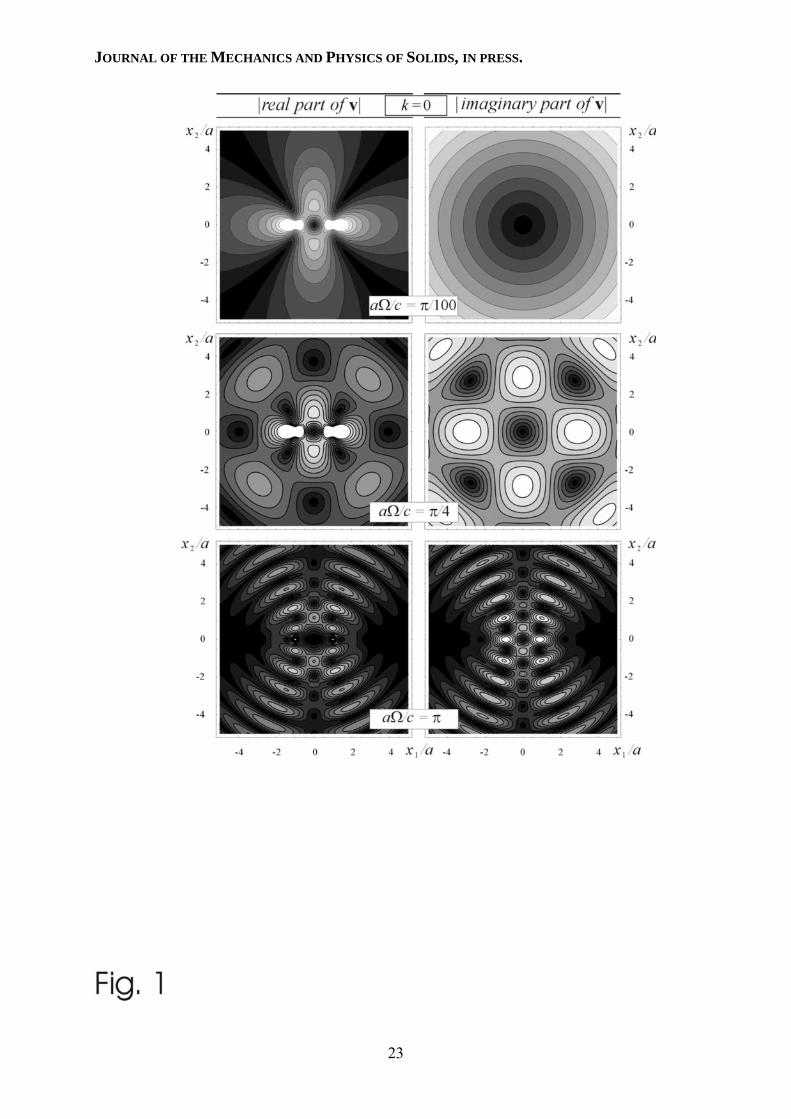
Level sets of the modulus of the real (left in the figure) and imaginary (right in the figure)
parts of the Green’s function for incremental displacements [eqn. (31) nondimensionalized
through multiplication by µ] are represented in the figures, in a region defined by the non-
dimensional coordinates x1/a and x2/a, where 2a is the distance between two unit forces
defining the dipole. Unless otherwise specified, the dipole is centred at the origin and aligned
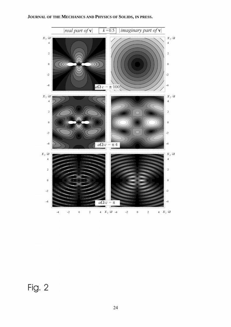
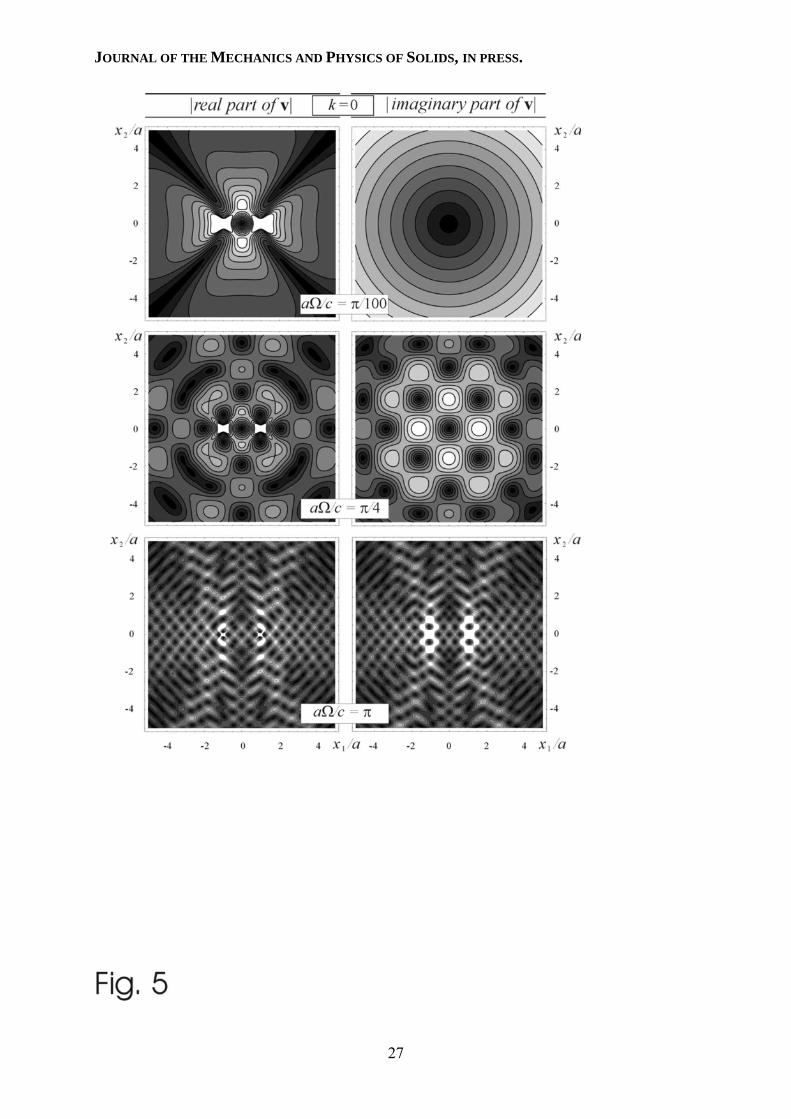
parallel to the x1-axis. Figs. 1-3, pertaining to Mooney-Rivlin material, are relative to
different values of the pre-stress parameter k. In particular, k = 0 [or λ = 1 from eqn. (41)3],
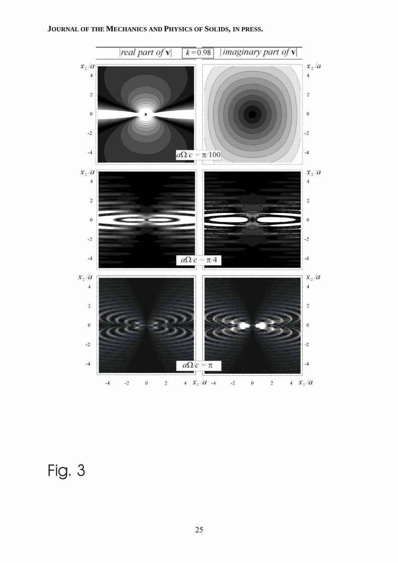
for Fig. 1; k = 0.5 [or λ ≅ 1.316 from eqn. (41)3], for Fig. 2; and k = 0.98 [or λ ≅ 3.154 from
eqn. (41)3], for Fig. 3.
In the quasi-static case, the displacement maps plotted in the dimensionless coordinates
x1/a and x2/a become independent of the dipole distance a. This is not true in the dynamic
case: the solution now depends on the dimensionless scale parameter
ca Ω =
1λπ2a , (42)
where λ1 corresponds to the wavelength of a plane wave propagating parallel to the x1-axis.
Therefore, parameter (42) can be viewed as a measure of the perturbation wavelength related
to the distance between the two forces forming the dipole.
The effects related to the changes in parameter (42) are systematically investigated, so
12
JOURNAL OF THE MECHANICS AND PHYSICS OF SOLIDS, IN PRESS.
that different parts of the same figures correspond (unless otherwise specified) to different
values of the parameter. In particular, all upper parts of Figs. 1-3 refer to a low frequency
limit, aΩ/c = π/100, so that the real part is coincident with the quasi-static solution reported
by Bigoni and Capuani (2002, their Fig. 3). The central parts of the figures correspond to
aΩ/c = π/4 and the lower parts to aΩ/c = π. Compared to Fig.1, we note anisotropy effects in
Fig. 2, where shear banding is not yet visible. However, the anisotropy dramatically affects
the propagation in Fig.3, where k = 0.98, a value relatively close to the loss of ellipticity. Here
shear band emergence interacts with wave propagation, creating a strong orientation (shear
bands become horizontal at the EI boundary) and focussing of the signal, which tends to
propagate only in the horizontal direction. The effect increases with frequency, so that at aΩ/c
= π, the width of shear bands becomes so narrow that the definition of the plot is not
sufficient to visualize displacement patterns, at least at the same scale of the other figures. In
this case, the signal almost does not propagate and therefore the displacement map remains
prevailingly dark. Specifically, according to eqn. (27), the propagation speeds in a Mooney-
Rivlin material (41) for plane waves travelling parallel to axes x1 and x2 are λ(µ0/ρ)1/2 and
(µ0/ρ)1/2/ λ, respectively. The former tends to infinity and the latter to zero when the elliptic
boundary is approached. In the particular case of aΩ/c = π/4 and k = 0.98, the wavelengths
characterizing propagation parallel to axes x1 and x2 are 8a and 0.80a, respectively. The
wavelength in the direction x2 is visible in the central part of Fig. 3 (where distance between
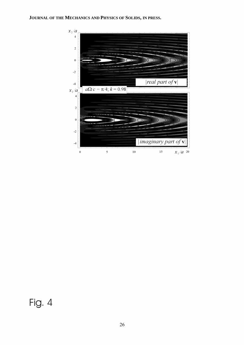
peaks correspond to one half of the wavelengths), whereas those along x1-axis become visible
in Fig. 4, which is an extension of Fig. 3 with x1/a ranging between 0 and 20. This figure
shows that wave patterns emanating from the dipole have an elliptical shape, whose aspect
ratio depends on the pre-stress parameter k. At increasing distance from the dipole, the
disturbances tend to propagate as plane waves travelling parallel to the x2-axis. Moreover, the
elliptical shapes tend to self-similarly decrease for increasing values of aΩ/c, thus explaining
the “shadowing effect” visible in the lower part of Fig. 3.
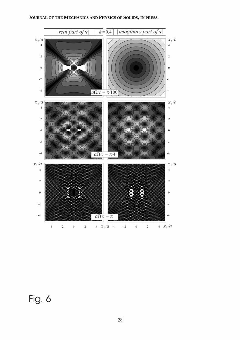
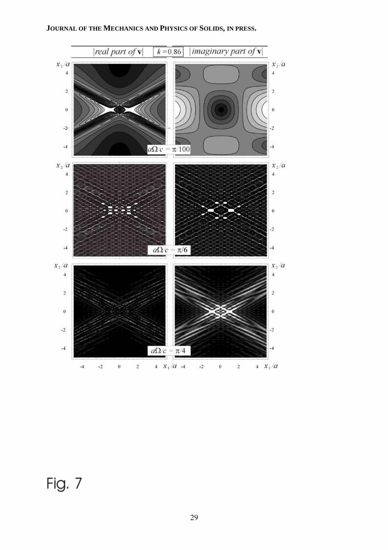
An anisotropic material with µ*/µ = 1/4 (in which failure of ellipticity occurs at k =
0.866) is considered in Figs. 5-8. The parameter k is now equal to 0 in Fig. 5, which therefore
corresponds to a orthotropic, incompressible material in the framework of the usual
infinitesimal theory of elasticity. We note that the effect of anisotropy is pretty evident, but it
is remarkably different from the situation near the boundary of loss of ellipticity, where the
13
JOURNAL OF THE MECHANICS AND PHYSICS OF SOLIDS, IN PRESS.
signal becomes localized in narrow “channels”. These are evident in Fig. 7 (corresponding to
k = 0.860), with inclination (±27.367°) corresponding to shear bands occurring at failure of
ellipticity. Fig. 6 pertains to the “intermediate” case of k = 0.4, where the pre-stress affects the
anisotropy of the material, but is still insufficient to trigger phenomena like those evidenced
near the elliptic boundary. Far from the dipole, the texture observed in the lower parts of Figs.
5 and 6 is generated by the intersection of two families of inclined wave patterns. Further, we
note that, while results relative to aΩ/c = π/100, π/4 and π are reported in Figs. 5 and 6, the
value aΩ/c = π/6 is considered in Fig. 7 instead of π since in this case the “shadowing effect”
prevails and almost nothing is visualized at the same scale of the other figures.
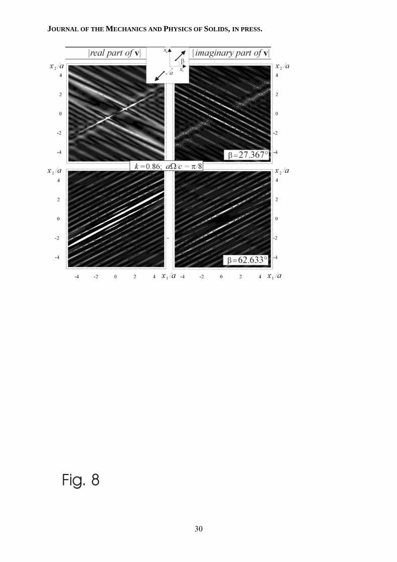
Investigation of the effects related to possible inclinations of the dipole with respect to
the principal stress reference system, also reveals interesting features (Fig. 8). We limit the
present discussion to examples pertaining to a dipole aligned parallel (β = 27.367°, Fig. 8
upper part) and orthogonal (β = 62.633°, Fig. 8 lower part) to the shear band that would occur
at the elliptic boundary. The quasi-static counterpart in the low-frequency limit may be found
in (Bigoni and Capuani, 2002, their Fig. 7). The frequency parameter aΩ/c has been selected
here equal to π/8 (upper part of the figures). It is interesting to note that a single family of
plane waves is generated in Fig. 8 (lower part), so that vibration tends to become focussed
into parallel layers.
Although restricted to plane, incompressible elasticity, it is considered unlikely that the
above conclusions are specific to the assumed constitutive model. Rather, we believe that the
above approach opens a new perspective to the analyses of material instability.
5. Integral representations for time-harmonic dynamics
For incremental problems consisting of dynamic time-harmonic deformation superimposed
upon a given homogeneous, pre-stressed (and equilibrated) state, it is possible to formulate
integral representations for incremental displacements vi and in-plane hydrostatic stress .
The procedure is strictly analogous to the quasi-static case for displacements, while it
becomes substantially different for the hydrostatic stress and yields a generalization to the
previous formulation given by Bigoni and Capuani (2002).
p&
14
JOURNAL OF THE MECHANICS AND PHYSICS OF SOLIDS, IN PRESS.
The importance of the boundary integral representations is that they provide (together
with the obtained Green’s function set) the basis for boundary element methods in nonlinear
elasticity, a possibility explored for the quasi-static case by Bigoni and Capuani (2002) and
Brun et al. (2003 a,b).
5.1 Boundary integral formulation for incremental displacements
Following the same procedure employed for the quasi-static case, but considering the
equations pertinent to the time-harmonic dynamics, one obtains for the incremental
displacement at point y of a generic body
[∫∂
−−−=B
xjigij
gjiij
gjj dlvntvntCv )()()( yxyxy && ] , (43)
where ∂B denotes the boundary of the body with outer unit normal ni; vi is the incremental
displacement; and ijt& gijt& are the incremental nominal stresses, associated with vi and ,
respectively. Finally, the matrix
giv
gjC still has the same definition as in the quasi-static case,
namely
∫∂
→−=
εε
Cxi
gij
gj dlntC )(lim
0yx& , (44)
where is a disk of radius ε centred at y. Since the dynamic Green’s function
asymptotically reduces to the quasi-static one as r → 0, the components of
εC
gjC are the same
as in the quasi-static case. For points y interior to the body, , while at a
smooth boundary point.
gjgjC δ= 2/gj
gjC δ=
5.2 Boundary integral formulation for in-plane incremental hydrostatic stress
As for the quasi-static case (Bigoni and Capuani, 2002), to establish an integral representation
for incremental hydrostatic stress we follow here a procedure which represents a
generalization of the technique employed by Ladyzhenskaya (1963) for two-dimensional
Stokes flow. In particular, a substitution of the constitutive equations (1) into the rate
equations of (time-harmonic) motion gives
hp,& = − ihkl vl,ki − ρΩ2 vh , (45)
which, used with the second gradient of (43) taken at interior points, yields
15
JOURNAL OF THE MECHANICS AND PHYSICS OF SOLIDS, IN PRESS.
∫∂
−=B
hp )(, y& nhsg xjig
snijg
snjiij dlvntvnt ])()([ ,, yxyx −−− && − ρΩ2vh . (46)
Noting that at interior points, x ≠ y, the following relationship holds
− = jhp,& nhsg
gsnjv , + ρΩ2 , (47) j
hv
where
ggg vp 1,12σ
+π= && , (48)
eqn. (46) becomes
=)(, yhp& ∫∂
−B
xghiig dlpnt )(, yx&& + ∫
∂B
nhsg + ρΩ2 , (49) xjig
snij dlvnt )(, yx −& ∫∂B
xjihij dlvnt )( yx −&
where is derived with respect to xghp,& h. By means of a procedure similar to that employed for
quasi-static deformation, the following expression for the gradient of the hydrostatic stress
increment can be obtained at a point y interior to the body
∫∫∂∂
−−=B
jiB
xghiigh vndlpntp )()( ,, yxy &&& ijkg x
ghk dlp )(, yx −&
∫∂
⎥⎦
⎤⎢⎣
⎡−
σ+µσ−−
σ−σµ−σµ+µ−µµ+
Bx
hii dlvvnv
,
211,2
111,1
2
*2** )()
2()()
2244( yxyx (50)
[ ]∫∂
−+−Ω+B
xh
hii dlpanv )()(2 yxyx &ρ ,
where 1 1 2
1 * 1,1 1,12( ) ( )a v v= µ − µ − σ + 2,1v 2,2v, . (51) 22 *2( )a = µ − µ
Let us now take if& = δigδ(x) in eqns. (6) written for the Green incremental displacement giv
and subtract the resulting eqn. (6)2, with g = 1, from eqn. (6)1, with g = 2. The following
identity results 1
1 ,2 2( ) (a p a p+ = +& 2,1)&
)
, (52)
showing that a potential W(x − y) can be introduced
, ( hh hW a p= + & , (53)
so that eqn. (50) can be integrated with respect to yh, yielding
∫∫∂∂
+−−=B
jiB
xg
iig vndlpntp )()( yxy &&& ijkg xgk dlp )(, yx −&
16
JOURNAL OF THE MECHANICS AND PHYSICS OF SOLIDS, IN PRESS.
∫∂
⎢⎣
⎡−⎟⎟
⎠
⎞⎜⎜⎝
⎛ σ−σµ−σµ+µ−µµ−
Bii vnv )(
2244 1
11,1
2
*2** yx (54)
xdlWv ⎥⎦⎤−Ω+−+− )()()
2( 22
11,2 yxyx ρσµσ ,
where ,gkp& is differentiated with respect to xk. It is worth noting that the fact that the signs of
eqn. (54) are opposite to those appearing in eqn. (50) is a consequence of integration with
respect to y. Equation (54) is an integral equation relating the in-plane hydrostatic stress
increment at interior points of the body to the boundary values of nominal traction and
displacement increments. Note that the term W contained in eqn. (54) (and which is absent in
the quasi-static counterpart) is not null even under the assumption of isotropy, µ = µ*, and
null pre-stress, k = 0. Moreover, the fact that the potential W is defined modulo an arbitrary
constant does not affect the boundary integral eqn. (54) since the flux of velocity vi through
any closed surface is null as a consequence of incompressibility.
To make eqn. (54) explicit, the expression for the potential W must be obtained. Let us
begin observing that it follows from eqn. (53) that 1 2 1 2 1
,1 ,2 * 1,1 2,2 1 2 ,12( )( ) ( )W W v v v v p p+ = µ − µ + − σ + + +& & 2 . (55)
Taking the plane wave expansion of function W
W = − 241π 1| =ω|
ω⋅ dW )(~ xω , (56)
eqn. (55) can be re-written as 1 2 1 2 1
1 2 * 1 1 2 2 1 1 2( ) 2( )( ) ( )W v v v v′ ′ω + ω = µ − µ ω + ω − σω + + +% % % % % % 2p p′ %
2⎤⎦
. (57)
Employing the incompressibility condition and the symmetry property = , eqn. (57) can
be integrated leading to
12v 2
1v
2* 2 24( )W v⎡= µ − µ ω − σ⎣
% % (ω⋅x) + log|ω⋅x|, (58)
where (ω⋅x) is given by eqn. (29). 22v%
Finally, eqn. (58) through eqn. (55) provides the potential W to be employed in the boundary
integral eqn. (54)
17
JOURNAL OF THE MECHANICS AND PHYSICS OF SOLIDS, IN PRESS.
W(r, ϑ) = − 1 log2
rc
Ωπ
− 12 (1 )k2
⎡⎢⎢π µ +⎢⎣
22*
0
4( )sin ( ) coslog cos ( )cos( ) ( )
r r dc c α
π ⎛ ⎞⎛ ⎞ µ − µ α + ϑ − σΩ Ω⎛ ⎞ + γ α + ϑ α⎜ ⎟⎜ ⎟⎜ ⎟ ⎜ ⎟Λ α + ϑ Λ + ϑ⎝ ⎠⎝ ⎠ ⎝ ⎠∫
α
/ 2 22*
0
4( )sin ( ) cos coscos ( ) log cos( ) ( ) ( )
r dc
π ⎛ ⎞ ⎛ ⎞µ − µ α + ϑ − σ α Ω α+ α + ϑ ⎜ ⎟ ⎜ ⎟⎜ ⎟ ⎜ ⎟Λ α + ϑ Λ α + ϑ Λ α + ϑ⎝ ⎠ ⎝ ⎠
∫ α
/ 2 22*
0
4( ) cos ( ) sin sinsin ( ) log cos( / 2) ( / 2) ( / 2)
r dc
π ⎛ ⎞ ⎛µ − µ α + ϑ − σ α Ω α+ α + ϑ ⎜ ⎟ ⎜⎜ ⎟ ⎜Λ α + ϑ + π Λ α + ϑ + π Λ α + ϑ + π⎝ ⎠ ⎝
∫⎞
α⎟⎟⎠
22*
0
4( )sin ( ) coscos ( )( ) ( )
r dc
π ⎛ ⎞µ − µ α + ϑ − σ Ω α+ α + ϑ α⎜ ⎟⎜ ⎟Λ α + ϑ Λ α + ϑ⎝ ⎠∫
22*
0
4( )sin ( ) coscos ( ) cos2 ( ) ( )
ri dc
σπ ⎤⎛ ⎞µ − µ α + ϑ −π Ω− α + ϑ ⎥⎜⎜Λ α + ϑ Λ α + ϑ ⎥⎝ ⎠ ⎦
∫α
α⎟⎟ . (59)
Since the potential W is defined modulo an arbitrary constant, we note that the term log(Ωr/c)
in eqn. (59) can be replaced by log r , with r denoting any dimensionless measure of distance.
In the particular case of isotropy, µ = µ*, and null pre-stress, k = 0, W reduces to
−log(Ωr/c)/(2π) and the boundary integral equation (54) with W given by eqn. (59) boils
down to that provided by Polyzos et al. (1998) and, in the quasi-static limit (ρΩ → 0), to that
obtained by Ladyzhenskaya (1963).
6. Conclusions
Time-harmonic dynamics of incremental nonlinear and incompressible elastic deformations
superimposed upon an arbitrary but homogeneous strain has been considered. The infinite-
body Green’s function set has been determined together with boundary integral equations for
incremental displacements and hydrostatic stress. These results provide the basis for boundary
element techniques in dynamic, nonlinear elasticity.
Employed as a dynamic perturbation, the Green’s function has revealed features of signal
propagation in a solid stretched until near the boundary of loss of ellipticity. Here the
propagation becomes highly localized along directions corresponding to the shear band
18
JOURNAL OF THE MECHANICS AND PHYSICS OF SOLIDS, IN PRESS.
inclinations found in the quasi-static limit. Even though this might have been anticipated, the
analytical determination of dynamic deformation maps provides a new point of view, which
for example may help in the design of filters for mechanical waves. Results presented in this
paper demonstrate that the proposed perturbative approach may become effective when
employed in, say, “non-standard situations”. In particular, we believe that the proposed
technique can be extended to a broad range of contexts, involving dynamics (for instance in
the analysis of flutter instability in a continuous medium, Piccolroaz et al. 2004),
nonhomogeneity (for instance shear bands formation in a nonuniform material) and
temperature effects (for instance analysis of adiabatic vs. isothermal shear banding).
Acknowledgements
D.B. gratefully acknowledges financial support from MURST-Cofin 2004 (Microstructural problems and models: applications in structural and civil engineering); D.C. thanks financial support from MURST-Cofin 2002 (2002084245_004).
19
JOURNAL OF THE MECHANICS AND PHYSICS OF SOLIDS, IN PRESS.
References
Bigoni, D., Capuani, D., 2002. Green’s function for incremental nonlinear elasticity: shear bands and boundary integral formulation. J. Mech. Phys. Solids 50, 471-500.
Bigoni, D., Petryk, H., 2002. A note on divergence and flutter instabilities in elastic-plastic materials. Int. J. Solids Struct. 39, 911-926.
Biot, M.A., 1965. Mechanics of Incremental Deformations. J. Wiley and Sons, New York.
Brun, M., Capuani, D., Bigoni, D. 2003 a. A boundary element technique for incremental, nonlinear elasticity. Part. I: Formulation. Comp. Meth. Appl. Mech. Eng. 192, 2003, 2461-2479.
Brun, M., Bigoni, D., Capuani, D., 2003 b. A boundary element technique for incremental, nonlinear elasticity. Part. II: Bifurcation and shear bands. Comp. Meth. Appl. Mech. Eng. 192, 2003, 2481-2499.
Gel’fand, I.M. and Shilov, G.E., 1964. Generalized Functions, vol. 1, Properties and Operations. Academic Press, New York.
Knowles, J.K., Sternberg, E. 1978. On the failure of ellipticity and the emergence of discontinuos deformation gradients in plane finite elastostatics. J. Elast. 8, 329-379.
Ladyzhenskaya, O.A., 1963. The Mathematical Theory of Viscous Incompressible Flow. Gordon and Breach, New York.
Merodio, J., Ogden, R.W., 2002. Material instabilities in fiber-reinforced nonlinearly elastic solids under plane deformation. Arch. Mech. 54, 525-552.
Merodio, J., Pence, T.H., 2001. Kink surfaces in a directionally reinforced neo-Hookean material under plane deformation: I Mechanical equilibrium. J. Elast. 62, 119-144.
Piccolroaz, A., Bigoni, D., Willis, J.R., 2005. A dynamical interpretation of flutter instability in a continuous medium. Submitted.
Polyzos, D., Tsinopulos, S.V., Beskos, D.E. 1998. Static and dynamic boundary element analysis in incompressible linear elasticity. Eur. J. Mech. A/Solids 17, 515-536.
Renardy, M., Rogers, R.C. 1993. An introduction to partial differential equations. Springer-Verlag, New York.
Willis, J.R., 1973. Self-similar problems in elastodynamics. Philosophical Trans. Royal Soc. London, Series A 274, 435-491.
Willis, J.R., 1991. Inclusions and cracks in constrained anisotropic media. In: Wu, J.J., Ting, T.C.T. and Barnett, D.M. (Eds.), Modern Theory of Anisotropic Elasticity and Applications. SIAM, Philadelphia, pp. 87-102.
20
JOURNAL OF THE MECHANICS AND PHYSICS OF SOLIDS, IN PRESS.
TIME-HARMONIC GREEN’S FUNCTION AND BOUNDARY INTEGRAL
FORMULATION FOR INCREMENTAL NONLINEAR ELASTICITY: DYNAMICS OF
WAVE PATTERNS AND SHEAR BANDS
D. Bigoni D. Capuani
FIGURE CAPTIONS Fig. 1. Level sets of the modulus of the real part (left) and imaginary part (right) of incremental displacement, for a time-harmonic pulsating dipole aligned with the x1-axis. A Mooney-Rivlin material is considered, with null pre-stress, k = 0. Effects of varying the frequency parameter aΩ/c are shown: low frequency aΩ/c = π/100 (upper part), aΩ/c = π/4 (central part) and high frequency aΩ/c = π (lower part). Fig. 2. Level sets of the modulus of the real part (left) and imaginary part (right) of incremental displacement, for a time-harmonic pulsating dipole aligned with the x1-axis. A Mooney-Rivlin material is considered, with a pre-stress k = 0.5, corresponding to a stretch λ=1.316. Effects of varying the frequency parameter aΩ/c are shown: low frequency aΩ/c = π/100 (upper part), aΩ/c = π/4 (central part) and high frequency aΩ/c = π (lower part). Fig. 3. Level sets of the modulus of the real part (left) and imaginary part (right) of incremental displacement, for a time-harmonic pulsating dipole aligned with the x1-axis. A Mooney- Rivlin material is considered, with a pre-stress k = 0.98, corresponding to a stretch λ=3.154, so that the material is near the elliptic boundary. Effects of varying the frequency parameter aΩ/c are shown: low frequency aΩ/c = π/100 (upper part), aΩ/c = π/4 (central part) and high frequency aΩ/c = π (lower part). Localized deformations are evident. Fig. 4. Level sets of the modulus of the real part (upper part) and imaginary part (lower part) of incremental displacement, for a time-harmonic pulsating dipole aligned with the x1- axis. A Mooney-Rivlin material is considered, as in the central part of Fig. 3: k = 0.98 and aΩ/c = π/4. The region x1/a ∈[0, 20] and x2/a ∈ [−5, 5] is considered. Fig. 5. Level sets of the modulus of the real part (left) and imaginary part (right) of incremental displacement, for a time-harmonic pulsating dipole aligned with the x1-axis. An anisotropic material with *µ /µ=1/4 and null pre-stress k = 0 is considered. Effects of varying the frequency parameter aΩ/c are shown: low frequency aΩ/c = π/100 (upper part), aΩ/c = π/4 (central part) and high frequency aΩ/c = π (lower part). Fig. 6. Level sets of the modulus of the real part (left) and imaginary part (right) of incremental displacement, for a time-harmonic pulsating dipole aligned with the x1-axis. An anisotropic material with /µ=1/4 and a pre-stress k = 0.4 is considered. Effects of *µ varying the frequency parameter aΩ/c are shown: low frequency aΩ/c = π/100 (upper part), aΩ/c = π/4 (central part) and high frequency aΩ/c = π (lower part).
21
JOURNAL OF THE MECHANICS AND PHYSICS OF SOLIDS, IN PRESS.
Fig. 7. Level sets of the modulus of the real part (left) and imaginary part (right) of incremental displacement, for a time-harmonic pulsating dipole aligned with the x1-axis. An anisotropic material with /µ=1/4 and a pre-stress k = 0.86 is considered near the *µ boundary of ellipticity. Effects of varying the frequency parameter aΩ/c are shown: low frequency aΩ/c = π/100 (upper part), aΩ/c = π/4 (central part) and high frequency aΩ/c = π (lower part). Localized deformations are evident. Fig. 8. Level sets of the modulus of the real part (left) and imaginary part (right) of incremental displacement, for a time-harmonic pulsating dipole inclined at angles 27.367° (upper part) and 62.633° (lower part) with respect to the x1-axis (i.e. the dipole is aligned parallel to the shear band evaluated at the elliptic boundary). An anisotropic material with /µ=1/4 and a pre-stress k = 0.86 is considered near the boundary of ellipticity and aΩ/c = π/8.
*µ
22
JOURNAL OF THE MECHANICS AND PHYSICS OF SOLIDS, IN PRESS.
23
JOURNAL OF THE MECHANICS AND PHYSICS OF SOLIDS, IN PRESS.
24
JOURNAL OF THE MECHANICS AND PHYSICS OF SOLIDS, IN PRESS.
25
JOURNAL OF THE MECHANICS AND PHYSICS OF SOLIDS, IN PRESS.
26
JOURNAL OF THE MECHANICS AND PHYSICS OF SOLIDS, IN PRESS.
27
JOURNAL OF THE MECHANICS AND PHYSICS OF SOLIDS, IN PRESS.
28
JOURNAL OF THE MECHANICS AND PHYSICS OF SOLIDS, IN PRESS.
29
JOURNAL OF THE MECHANICS AND PHYSICS OF SOLIDS, IN PRESS.
30