Time of Concentration - iowasudas.org 2 - Stormwater Section 2B-3 - Time of Concentration 2 Revised: 2013 Edition C. NRCS Velocity Method The NRCS Velocity method is described in full

2B-3

Design Manual

Chapter 2 - Stormwater

2B - Urban Hydrology and Runoff

1 Revised: 2013 Edition

Time of Concentration

A. Introduction

Time of concentration (Tc) is the time required for runoff to travel from the hydraulically most distant

point in the watershed to the outlet. The hydraulically most distant point is the point with the longest

travel time to the watershed outlet, and not necessarily the point with the longest flow distance to the

outlet.

Time of concentration is a critical component in some analysis methods for calculating peak

discharge from an area. The peak discharge occurs when all segments of the drainage area are

contributing to the runoff from the site.

There are many methods available to estimate the time of concentration including the Kirpich

formula, Kerby formula, NRCS Velocity Method, and NRCS Lag Method. The NRCS Velocity and

Lag methods are two of the most commonly used methods for determining time of concentration and

are described below.

B. Factors Affecting Time of Concentration

1. Surface Roughness: One of the most significant effects of urban development on overland flow

is the lowering of retardance to flow causing higher velocities. Undeveloped areas with very

slow and shallow overland flow (sheet flow and shallow concentrated flow) through vegetation

become modified by urban development. Flow is then delivered to streets, gutters, and storm

sewers that transport runoff downstream more rapidly. Travel time through the watershed is

generally decreased.

2. Channel Shape: In small non-urban watersheds, much of the travel time results from overland

flow in upstream areas. Typically, urbanization reduces overland flow lengths by conveying

storm runoff into a channel as soon as possible. Since channel designs have efficient hydraulic

characteristics, runoff flow velocity increases and travel time decreases.

3. Slope: Slopes may be increased or decreased by urbanization, depending on the extent of site

grading or the extent to which storm sewers and street ditches are used in the design of the water

management system. Slope will tend to increase when channels are straightened and decrease

when overland flow is directed through storm sewers, street gutters, and diversions

Urbanization usually decreases time of concentration, thereby increasing the peak discharge.

However, time of concentration can be increased as a result of ponding behind small or

inadequate drainage systems (including inlets and road culverts) or by reduction of land slope

through grading.

Chapter 2 - Stormwater Section 2B-3 - Time of Concentration


C. NRCS Velocity Method

The NRCS Velocity method is described in full detail in NRCS TR-55.

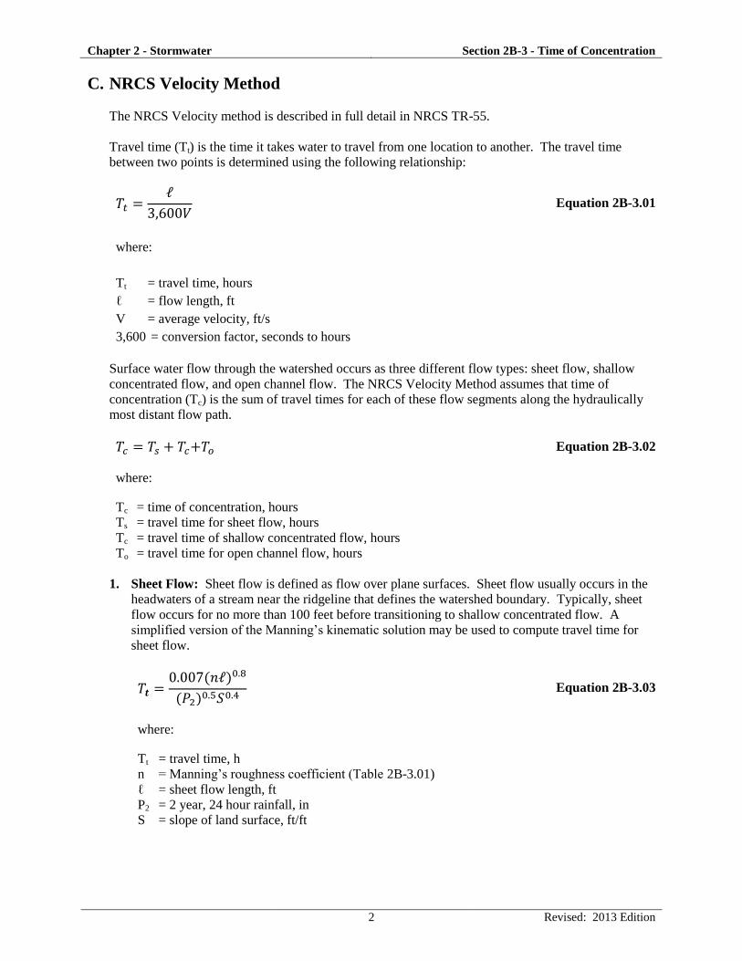
Travel time (Tt) is the time it takes water to travel from one location to another. The travel time

between two points is determined using the following relationship:

Equation 2B-3.01

where:

Tt = travel time, hours

ℓ = flow length, ft

V = average velocity, ft/s

3,600 = conversion factor, seconds to hours

Surface water flow through the watershed occurs as three different flow types: sheet flow, shallow

concentrated flow, and open channel flow. The NRCS Velocity Method assumes that time of

concentration (Tc) is the sum of travel times for each of these flow segments along the hydraulically

most distant flow path.

Equation 2B-3.02

where:

Tc = time of concentration, hours

Ts = travel time for sheet flow, hours

Tc = travel time of shallow concentrated flow, hours

To = travel time for open channel flow, hours

1. Sheet Flow: Sheet flow is defined as flow over plane surfaces. Sheet flow usually occurs in the

headwaters of a stream near the ridgeline that defines the watershed boundary. Typically, sheet

flow occurs for no more than 100 feet before transitioning to shallow concentrated flow. A

simplified version of the Manning’s kinematic solution may be used to compute travel time for

sheet flow.

Equation 2B-3.03

where:

Tt = travel time, h

n = Manning’s roughness coefficient (Table 2B-3.01)

ℓ = sheet flow length, ft

P2 = 2 year, 24 hour rainfall, in

S = slope of land surface, ft/ft



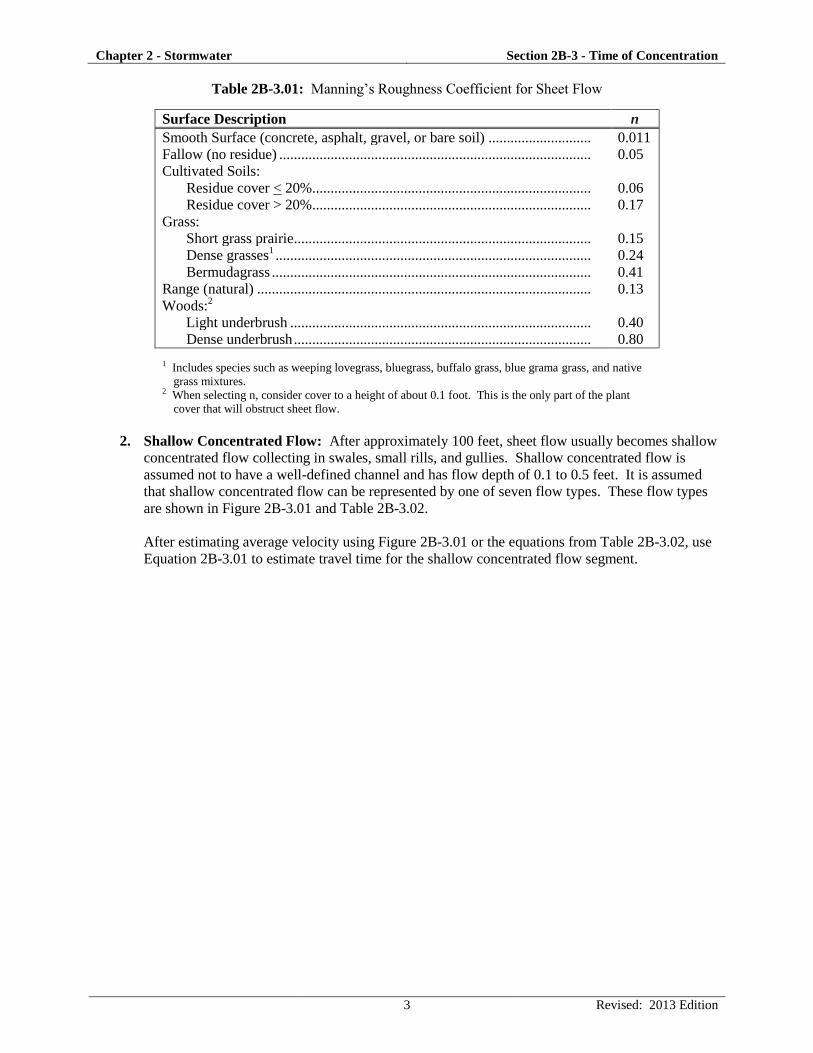
Table 2B-3.01: Manning’s Roughness Coefficient for Sheet Flow

Surface Description n

Smooth Surface (concrete, asphalt, gravel, or bare soil) ............................ 0.011

Fallow (no residue) ..................................................................................... 0.05

Cultivated Soils:

Residue cover < 20% ............................................................................ 0.06

Residue cover > 20% ............................................................................ 0.17

Grass:

Short grass prairie ................................................................................. 0.15

Dense grasses1 ...................................................................................... 0.24

Bermudagrass ....................................................................................... 0.41

Range (natural) ........................................................................................... 0.13

Woods:2

Light underbrush .................................................................................. 0.40

Dense underbrush ................................................................................. 0.80

1 Includes species such as weeping lovegrass, bluegrass, buffalo grass, blue grama grass, and native

grass mixtures. 2 When selecting n, consider cover to a height of about 0.1 foot. This is the only part of the plant

cover that will obstruct sheet flow.

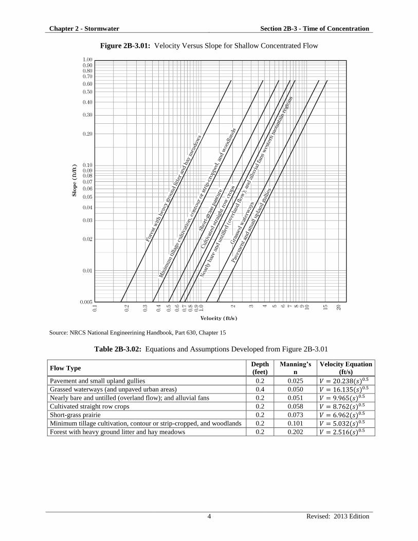
2. Shallow Concentrated Flow: After approximately 100 feet, sheet flow usually becomes shallow

concentrated flow collecting in swales, small rills, and gullies. Shallow concentrated flow is

assumed not to have a well-defined channel and has flow depth of 0.1 to 0.5 feet. It is assumed

that shallow concentrated flow can be represented by one of seven flow types. These flow types

are shown in Figure 2B-3.01 and Table 2B-3.02.

After estimating average velocity using Figure 2B-3.01 or the equations from Table 2B-3.02, use

Equation 2B-3.01 to estimate travel time for the shallow concentrated flow segment.



Figure 2B-3.01: Velocity Versus Slope for Shallow Concentrated Flow

Source: NRCS National Engineerining Handbook, Part 630, Chapter 15

Table 2B-3.02: Equations and Assumptions Developed from Figure 2B-3.01

Flow Type Depth

(feet)

Manning’s

n

Velocity Equation

(ft/s)

Pavement and small upland gullies 0.2 0.025

Grassed waterways (and unpaved urban areas) 0.4 0.050

Nearly bare and untilled (overland flow); and alluvial fans 0.2 0.051

Cultivated straight row crops 0.2 0.058

Short-grass prairie 0.2 0.073

Minimum tillage cultivation, contour or strip-cropped, and woodlands 0.2 0.101

Forest with heavy ground litter and hay meadows 0.2 0.202



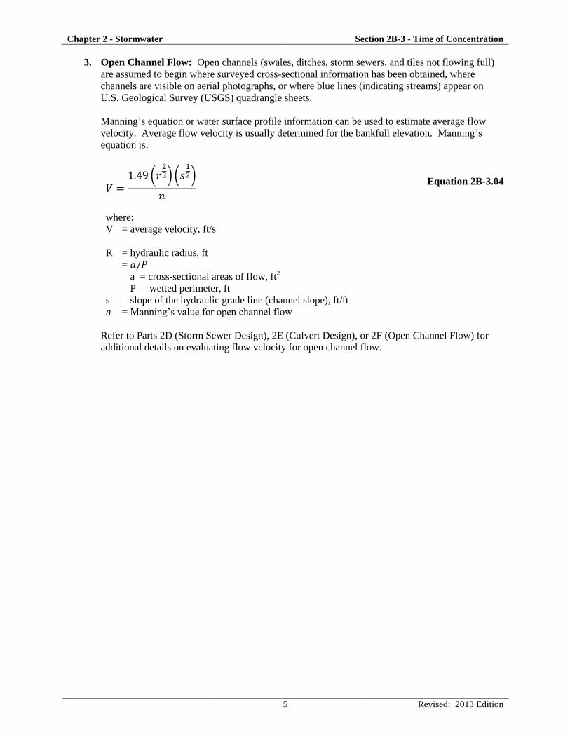
3. Open Channel Flow: Open channels (swales, ditches, storm sewers, and tiles not flowing full)

are assumed to begin where surveyed cross-sectional information has been obtained, where

channels are visible on aerial photographs, or where blue lines (indicating streams) appear on

U.S. Geological Survey (USGS) quadrangle sheets.

Manning’s equation or water surface profile information can be used to estimate average flow

velocity. Average flow velocity is usually determined for the bankfull elevation. Manning’s

equation is:

(

) (

)

Equation 2B-3.04

where:

V = average velocity, ft/s

R = hydraulic radius, ft

=

a = cross-sectional areas of flow, ft2

P = wetted perimeter, ft

s = slope of the hydraulic grade line (channel slope), ft/ft

n = Manning’s value for open channel flow

Refer to Parts 2D (Storm Sewer Design), 2E (Culvert Design), or 2F (Open Channel Flow) for

additional details on evaluating flow velocity for open channel flow.



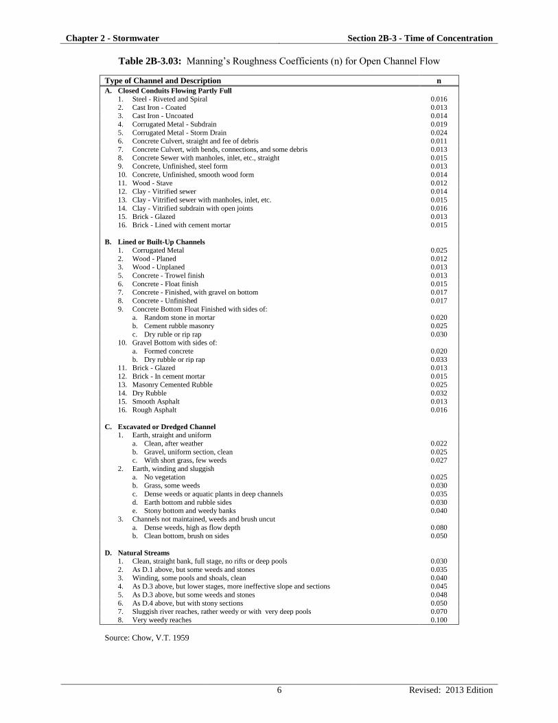
Table 2B-3.03: Manning’s Roughness Coefficients (n) for Open Channel Flow

Type of Channel and Description n

A. Closed Conduits Flowing Partly Full

1. Steel - Riveted and Spiral 0.016

2. Cast Iron - Coated 0.013 3. Cast Iron - Uncoated 0.014

4. Corrugated Metal - Subdrain 0.019

5. Corrugated Metal - Storm Drain 0.024 6. Concrete Culvert, straight and fee of debris 0.011

7. Concrete Culvert, with bends, connections, and some debris 0.013

8. Concrete Sewer with manholes, inlet, etc., straight 0.015 9. Concrete, Unfinished, steel form 0.013

10. Concrete, Unfinished, smooth wood form 0.014

11. Wood - Stave 0.012 12. Clay - Vitrified sewer 0.014

13. Clay - Vitrified sewer with manholes, inlet, etc. 0.015

14. Clay - Vitrified subdrain with open joints 0.016 15. Brick - Glazed 0.013

16. Brick - Lined with cement mortar 0.015

B. Lined or Built-Up Channels

1. Corrugated Metal 0.025

2. Wood - Planed 0.012 3. Wood - Unplaned 0.013

5. Concrete - Trowel finish 0.013

6. Concrete - Float finish 0.015 7. Concrete - Finished, with gravel on bottom 0.017

8. Concrete - Unfinished 0.017

9. Concrete Bottom Float Finished with sides of: a. Random stone in mortar 0.020

b. Cement rubble masonry 0.025

c. Dry ruble or rip rap 0.030 10. Gravel Bottom with sides of:

a. Formed concrete 0.020

b. Dry rubble or rip rap 0.033 11. Brick - Glazed 0.013

12. Brick - In cement mortar 0.015 13. Masonry Cemented Rubble 0.025

14. Dry Rubble 0.032

15. Smooth Asphalt 0.013 16. Rough Asphalt 0.016

C. Excavated or Dredged Channel 1. Earth, straight and uniform

a. Clean, after weather 0.022

b. Gravel, uniform section, clean 0.025 c. With short grass, few weeds 0.027

2. Earth, winding and sluggish

a. No vegetation 0.025 b. Grass, some weeds 0.030

c. Dense weeds or aquatic plants in deep channels 0.035

d. Earth bottom and rubble sides 0.030 e. Stony bottom and weedy banks 0.040

3. Channels not maintained, weeds and brush uncut

a. Dense weeds, high as flow depth 0.080 b. Clean bottom, brush on sides 0.050

D. Natural Streams 1. Clean, straight bank, full stage, no rifts or deep pools 0.030

2. As D.1 above, but some weeds and stones 0.035

3. Winding, some pools and shoals, clean 0.040 4. As D.3 above, but lower stages, more ineffective slope and sections 0.045

5. As D.3 above, but some weeds and stones 0.048

6. As D.4 above, but with stony sections 0.050 7. Sluggish river reaches, rather weedy or with very deep pools 0.070

8. Very weedy reaches 0.100

Source: Chow, V.T. 1959



D. NRCS Lag Method

In drainage basins where a large segment of the area is rural in character and has long hydraulic

length, the potential for retention of rainfall on the watershed increases along with travel time. Under

these conditions, the NRCS lag method may be used since it includes most of the factors to estimate

travel time and thus time of concentration.

The NRCS lag method was developed from observations of agricultural watersheds where overland

flow paths are poorly defined and channel flow is absent. However, it has been adapted to small

urban watersheds less than 2,000 acres. For situations where the lag method is used in urban areas, an

adjustment factor needs to be applied to the results to account for the effects of urbanization. This

adjustment is described in number 5 below. The method performs reasonably well for completely

paved areas, but performs poorly when channel flow (including storm sewers) is a significant part of

the time of concentration.

Lag is the delay between the time runoff from a rainfall event over a watershed begins until runoff

reaches its maximum peak. Lag is a function of the flow length of the watershed, average land slope

of the watershed, and the potential maximum retention of rainfall on the watershed.

1. Flow Length of Watershed: The flow length of the watershed, ℓ, is the length from the point of

design along the main channel to the ridgeline at the upper end of the watershed. Moving

upstream, the main channel may appear to divide into two channels at several points along its

length. The main channel is then defined as the channel that drains the greater tributary drainage

area. This same definition is used for all further upstream channel divisions until the watershed

ridgeline is reached.

Since many channels meander through their floodplains and since most designs are based on

floods that exceed channel capacity, the proper channel length to use is actually the length along

the valley; i.e., the channel meanders should be ignored.

2. Average Watershed Slope: The average watershed land slope, Y, is estimated using one of the

two methods described below. Average watershed slope is a variable, which is usually not

readily apparent. Therefore, a systematic procedure for finding slope is desirable. Several

observations or map measurements are commonly needed. Care should be taken in determining

this parameter as the time of concentration (and subsequently the peak discharge and hydrograph

shape) is sensitive to the value used for watershed slope. Best hydrologic results are obtained

when the slope value represents a weighted average for the area. Two methods for computing

slope are demonstrated in example exercises below.

3. Maximum Potential Retention: The parameter S represents the potential maximum moisture

retention of the soil and is related to soil and cover conditions of the watershed. It is empirically-

determined using the SCS curve number (CN), which is provided in Tables 2B-4.03 through 2B-

4.05 in Section 2B-4.



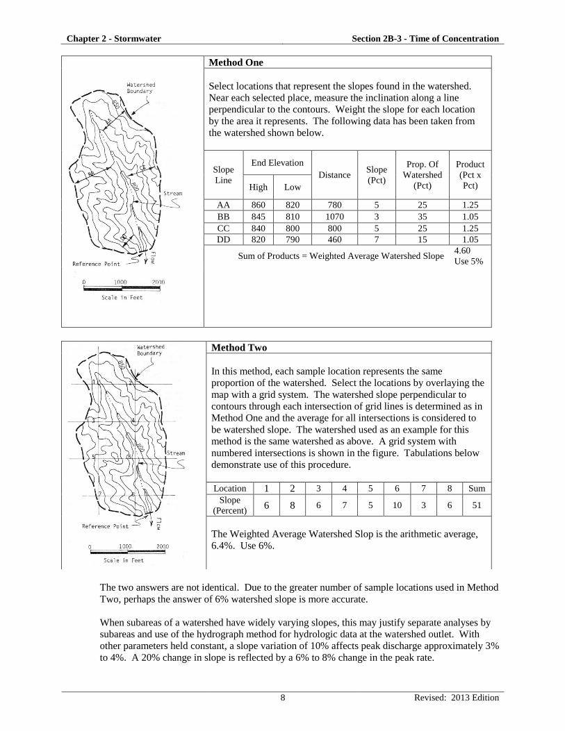
Method One

Select locations that represent the slopes found in the watershed.

Near each selected place, measure the inclination along a line

perpendicular to the contours. Weight the slope for each location

by the area it represents. The following data has been taken from

the watershed shown below.

Slope

Line

End Elevation

Distance Slope

(Pct)

Prop. Of

Watershed

(Pct)

Product

(Pct x

Pct) High Low

AA 860 820 780 5 25 1.25

BB 845 810 1070 3 35 1.05

CC 840 800 800 5 25 1.25

DD 820 790 460 7 15 1.05

Sum of Products = Weighted Average Watershed Slope 4.60

Use 5%

The two answers are not identical. Due to the greater number of sample locations used in Method

Two, perhaps the answer of 6% watershed slope is more accurate.

When subareas of a watershed have widely varying slopes, this may justify separate analyses by

subareas and use of the hydrograph method for hydrologic data at the watershed outlet. With

other parameters held constant, a slope variation of 10% affects peak discharge approximately 3%

to 4%. A 20% change in slope is reflected by a 6% to 8% change in the peak rate.

Method Two

In this method, each sample location represents the same

proportion of the watershed. Select the locations by overlaying the

map with a grid system. The watershed slope perpendicular to

contours through each intersection of grid lines is determined as in

Method One and the average for all intersections is considered to

be watershed slope. The watershed used as an example for this

method is the same watershed as above. A grid system with

numbered intersections is shown in the figure. Tabulations below

demonstrate use of this procedure.

Location 1 2 3 4 5 6 7 8 Sum

Slope

(Percent) 6 8 6 7 5 10 3 6 51

The Weighted Average Watershed Slop is the arithmetic average,

6.4%. Use 6%.



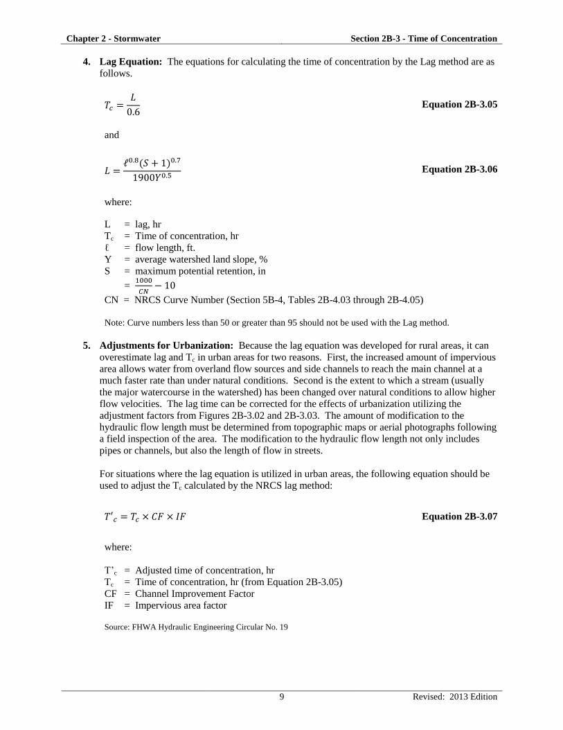
4. Lag Equation: The equations for calculating the time of concentration by the Lag method are as

follows.

Equation 2B-3.05

and

Equation 2B-3.06

where:

L = lag, hr

Tc = Time of concentration, hr

ℓ = flow length, ft.

Y = average watershed land slope, %

S = maximum potential retention, in

=

CN = NRCS Curve Number (Section 5B-4, Tables 2B-4.03 through 2B-4.05)

Note: Curve numbers less than 50 or greater than 95 should not be used with the Lag method.

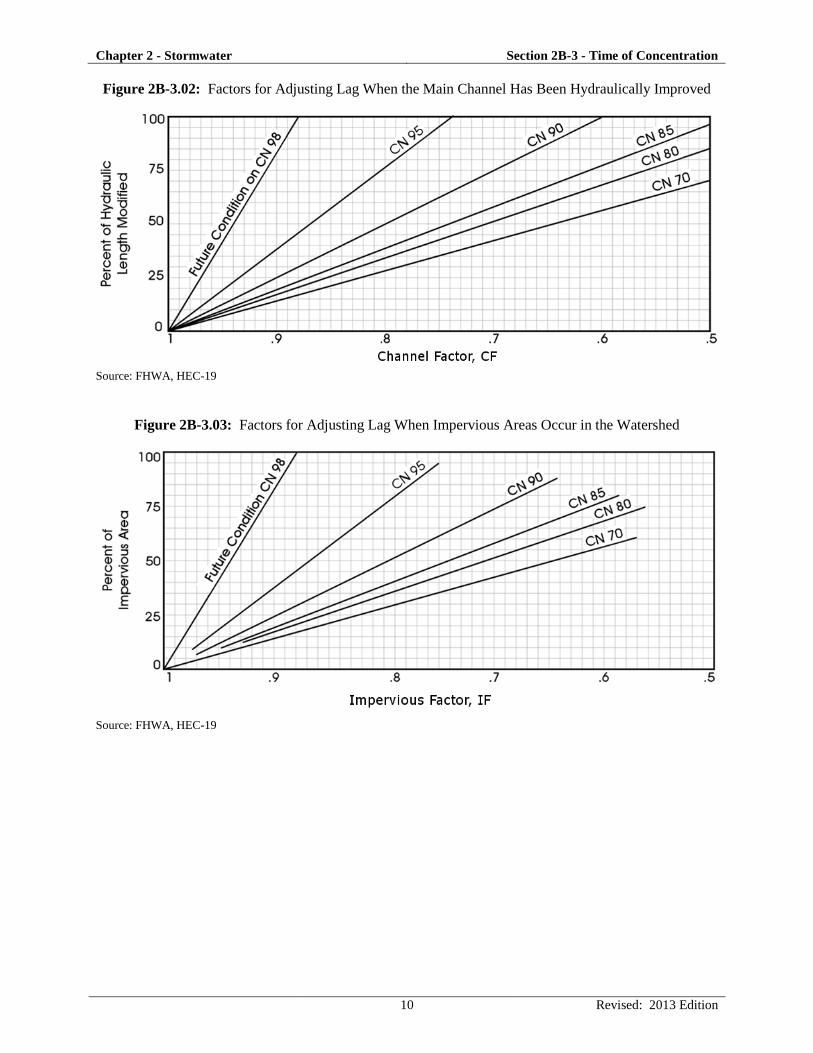
5. Adjustments for Urbanization: Because the lag equation was developed for rural areas, it can

overestimate lag and Tc in urban areas for two reasons. First, the increased amount of impervious

area allows water from overland flow sources and side channels to reach the main channel at a

much faster rate than under natural conditions. Second is the extent to which a stream (usually

the major watercourse in the watershed) has been changed over natural conditions to allow higher

flow velocities. The lag time can be corrected for the effects of urbanization utilizing the

adjustment factors from Figures 2B-3.02 and 2B-3.03. The amount of modification to the

hydraulic flow length must be determined from topographic maps or aerial photographs following

a field inspection of the area. The modification to the hydraulic flow length not only includes

pipes or channels, but also the length of flow in streets.

For situations where the lag equation is utilized in urban areas, the following equation should be

used to adjust the Tc calculated by the NRCS lag method:

Equation 2B-3.07

where:

T’c = Adjusted time of concentration, hr

Tc = Time of concentration, hr (from Equation 2B-3.05)

CF = Channel Improvement Factor

IF = Impervious area factor Source: FHWA Hydraulic Engineering Circular No. 19



Figure 2B-3.02: Factors for Adjusting Lag When the Main Channel Has Been Hydraulically Improved

Source: FHWA, HEC-19

Figure 2B-3.03: Factors for Adjusting Lag When Impervious Areas Occur in the Watershed

Source: FHWA, HEC-19



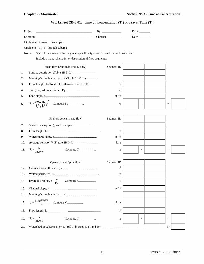
Worksheet 2B-3.01: Time of Concentration (Tc) or Travel Time (Tt)

Project _____________________________________ By _____________ Date _______

Location _____________________________________ Checked _________ Date _______

Circle one: Present Developed

Circle one: Tc Tt through subarea

Notes: Space for as many as two segments per flow type can be used for each worksheet.

Include a map, schematic, or description of flow segments.

Sheet flow (Applicable to Tc only) Segment ID

1. Surface description (Table 2B-3.01)……………………

2. Manning’s roughness coeff., n (Table 2B-3.01)…………

3. Flow Length, L (Total L less than or equal to 300’)… ft

4. Two year, 24 hour rainfall, P2……………………………. in

5. Land slope, s………………………………………………. ft / ft

6.

4.02

8.0

tsP

nL007.0T Compute Tt…………….. hr + =

Shallow concentrated flow Segment ID

7. Surface description (paved or unpaved)………………..

8. Flow length, L……………………………………………… ft

9. Watercourse slope, s……………………………………... ft / ft

10. Average velocity, V (Figure 2B-3.01)…………………… ft / s

11. V3600

LTt Compute Tt…………….. hr + =

Open channel / pipe flow Segment ID

12. Cross sectional flow area, a……………………………... ft2

13. Wetted perimeter, Pw.…………………………………….. ft

14. Hydraulic radius, wP

ar Compute r……………… ft

15. Channel slope, s………………………………………….. ft / ft

16. Manning’s roughness coeff., n…………………………...

17. n

sr49.1V

2132

Compute V……………... ft / s

18. Flow length, L……………………………………………… ft

19. V3600

LTt Compute Tt…………….. hr + =

20. Watershed or subarea Tc or Tt (add Tt in steps 6, 11 and 19)………………………………………… hr



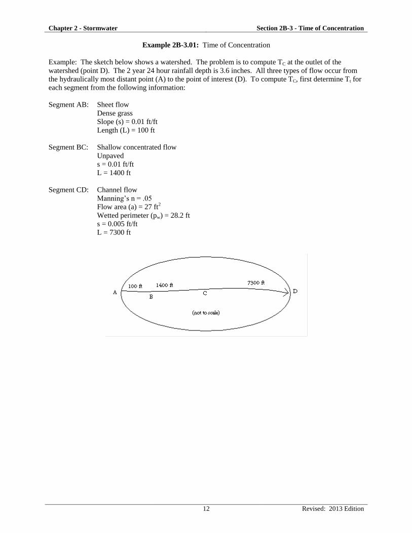
Example 2B-3.01: Time of Concentration

Example: The sketch below shows a watershed. The problem is to compute TC at the outlet of the

watershed (point D). The 2 year 24 hour rainfall depth is 3.6 inches. All three types of flow occur from

the hydraulically most distant point (A) to the point of interest (D). To compute TC, first determine Tt for

each segment from the following information:

Segment AB: Sheet flow

Dense grass

Slope (s) = 0.01 ft/ft

Length (L) = 100 ft

Segment BC: Shallow concentrated flow

Unpaved

s = 0.01 ft/ft

L = 1400 ft

Segment CD: Channel flow

Manning’s n = .05

Flow area (a) = 27 ft2

Wetted perimeter (pw) = 28.2 ft

s = 0.005 ft/ft

L = 7300 ft



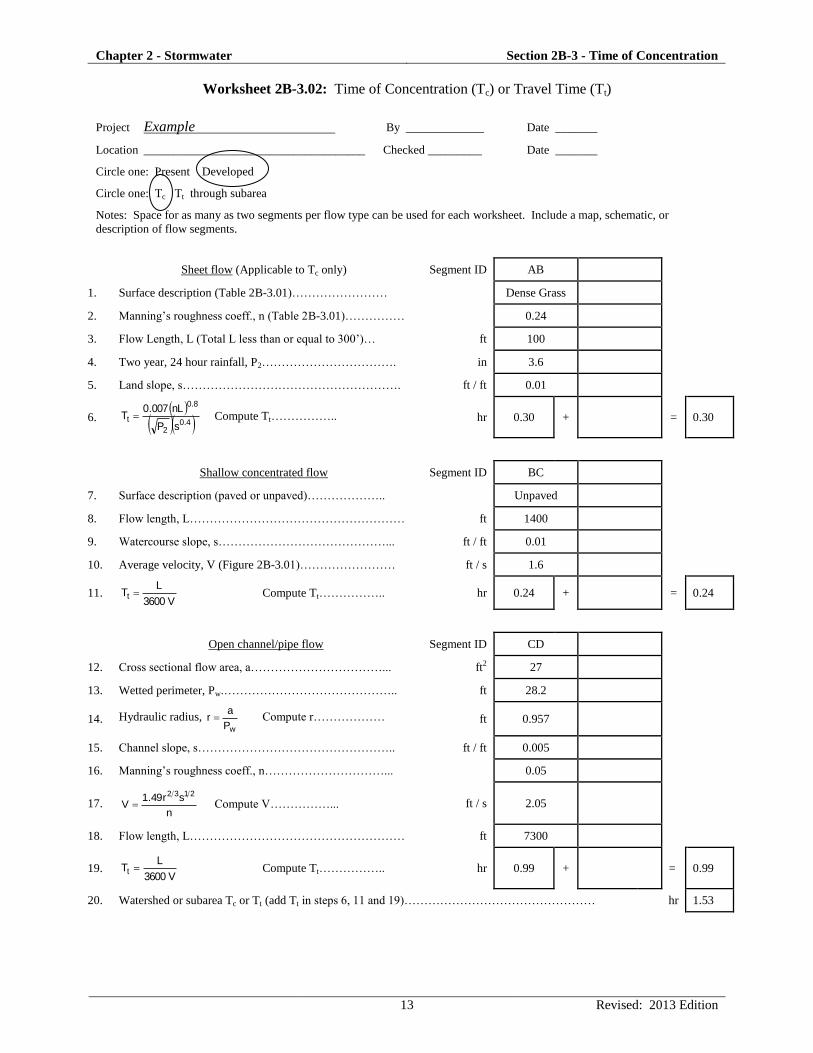
Worksheet 2B-3.02: Time of Concentration (Tc) or Travel Time (Tt)

Project Example By _____________ Date _______

Location _____________________________________ Checked _________ Date _______

Circle one: Present Developed

Circle one: Tc Tt through subarea

Notes: Space for as many as two segments per flow type can be used for each worksheet. Include a map, schematic, or

description of flow segments.

Sheet flow (Applicable to Tc only) Segment ID AB

1. Surface description (Table 2B-3.01)…………………… Dense Grass

2. Manning’s roughness coeff., n (Table 2B-3.01)…………… 0.24

3. Flow Length, L (Total L less than or equal to 300’)… ft 100

4. Two year, 24 hour rainfall, P2……………………………. in 3.6

5. Land slope, s………………………………………………. ft / ft 0.01

6.

4.02

8.0

tsP

nL007.0T Compute Tt…………….. hr 0.30 + = 0.30

Shallow concentrated flow Segment ID BC

7. Surface description (paved or unpaved)……………….. Unpaved

8. Flow length, L……………………………………………… ft 1400

9. Watercourse slope, s……………………………………... ft / ft 0.01

10. Average velocity, V (Figure 2B-3.01)…………………… ft / s 1.6

11. V3600

LTt Compute Tt…………….. hr 0.24 + = 0.24

Open channel/pipe flow Segment ID CD

12. Cross sectional flow area, a……………………………... ft2 27

13. Wetted perimeter, Pw.…………………………………….. ft 28.2

14. Hydraulic radius, wP

ar Compute r……………… ft 0.957

15. Channel slope, s………………………………………….. ft / ft 0.005

16. Manning’s roughness coeff., n…………………………... 0.05

17. n

sr49.1V

2132

Compute V……………... ft / s 2.05

18. Flow length, L……………………………………………… ft 7300

19. V3600

LTt Compute Tt…………….. hr 0.99 + = 0.99

20. Watershed or subarea Tc or Tt (add Tt in steps 6, 11 and 19)………………………………………… hr 1.53



E. References

Chow, V.T. Open Channel Hydraulics. 1959.

U.S. Department of Transportation. Hydraulic Engineering Circular No. 19: Hydrology. 1984.

USDA Natural Resource Conservation Service. National Engineering Handbook - Part 630. Chapter

15: Time of Concentration. 2010.

Documents

Time of Concentration - iowasudas.org 2 - Stormwater Section 2B-3 - Time of Concentration 2 Revised: 2013 Edition C. NRCS Velocity Method The NRCS Velocity method is described in full