Embed Size (px)
Citation preview

TIME: PERCEPTION AND DECISION-MAKING
by
Vijay Mohan K Namboodiri
A dissertation submitted to Johns Hopkins University
In conformity with the requirements for the Doctor of Philosophy
Baltimore, Maryland
February, 2015
© Vijay Mohan K Namboodiri
All Rights Reserved

ii
To Bhavadasan Bhattathiripad, my grandfather

iii
Abstract
Answering how animal brains measure the passage of time, and, make decisions about
the timing of rewards (e.g. smaller-sooner versus larger-later) is crucial for understanding
normal and clinically-impulsive behavior. This thesis attempts to further our
understanding of these questions using both experimental and theoretical approaches.
In the first part of my thesis, I developed a visually-cued interval timing task that required
rats to decide when to perform an action following a brief visual stimulus. Using single-
unit recordings and optogenetics in this task, I showed that activity generated by the
primary visual cortex (V1) embodies the target interval and instructs the decision to time
the action on a trial-by-trial basis. A spiking neuronal model of local recurrent
connections in V1 produced neural responses that predict and drive the timing of future
actions, consistent with the experimental observations. My data demonstrate that the
primary visual cortex contributes to instructing the timing of visually-cued actions.
In the second part of my thesis, I theoretically address the question of how animals and
humans perceive delays to rewards and decide about such delayed rewards. Humans, as
with other animals, decide between courses of action based on the evaluation of the
relative worth of expected outcomes. How outcome magnitude interacts with temporal
delay, however, has yet eluded a principled understanding that reconciles the breadth of
well-established behaviors in intertemporal decision-making. I first review the history of
this endeavor to rationalize decision-making regarding the domain of time, highlighting
extant theories, their limitations, and recent experimental advances. I then propose a

iv
simple theoretical solution to this problem. My theory recasts long presumed deficiencies
in observed decision-making behavior, not as flaws, but rather as signs of optimal
decision-making under experiential constraints. This new conception naturally unites the
fields of intertemporal decision-making and time perception, which have long been
recognized to be interconnected but not yet unified in a formal framework.
I extend the results of my theoretical work in the third part and show analytically that the
perception of reward magnitude, time, and subjective value change all approximately
obey Weber’s law.

v
Thesis Readers Marshall G Hussain Shuler, Ph.D., (Advisor), Assistant Professor, Dept. of Neuroscience
James J Knierim, Ph.D., Professor, Dept. of Neuroscience

vi
Preface
First and foremost, I want to thank my parents for bringing me into this world and for all
the love and support that they have provided me over the years. I am positive that if not
for their guidance, I would be far less responsible, far less motivated and far less
compassionate. I don’t think that my love, respect and gratitude for them could ever be
translated into words and hence, such an attempt will not be made. In the same breath that
I thank my parents, I would also like to thank my sister. Everything I said about my
feelings for my parents is also true about my feelings for her. Next, I would like to thank
my maternal grandfather, who always had a simple expectation from me: to be the best in
whatever I do. Regardless of whether it’s my high school class or college or a national
exam, he would always be disappointed if I wasn’t the best. Needless to say, he has been
disappointed many times. But I hope that if he was still alive, he would be proud of this
thesis. I would like to also thank all of my teachers (that taught me right from
kindergarten to graduate school) that molded me into the person I am today. I am grateful
to Steve Hsiao and King Wai Yau for believing in me and giving me the chance to be a
part of the Hopkins neuroscience family. I also am grateful to Rita Ragan and Beth Wood
Roig for all their support during my graduate school. I thank Ernst Niebur and Rudiger
von der Heydt for agreeing to take me on as a rotation student and giving me part of my
foundational research training. I would also like to thank my undergraduate research
mentor, Rohit Manchanda, for introducing me formally to the field of computational
neuroscience.

vii
I am thankful for my thesis committee members James Knierim, David Foster and Ernst
Niebur for guiding my project from its initial stages. I am, of course, especially thankful
to my mentor, Marshall Hussain Shuler, for everything that he has done for me over this
long journey. He provided me with a rich, intellectual and nurturing environment in
which I could really explore countless ideas. To me, he has been the perfect guide,
providing me with just the right mix of independence and intellectual support. This
freedom to explore my own ideas largely shaped the trajectory of my theoretical work. In
his lab, I owe so much of my early growth to Emma Roach and Camila Zold. Without
their support, my experimental work would have severely diminished in quality. I also
thank Tanya Marton and Joshua Levy for countless hours of intellectual discussions and
their scientific curiosity, rigor and support. Tanya, especially deserves special mention
for asking the right (but tough) questions that spawned my theoretical work. More
importantly, I thank Emma, Camila, Tanya and Josh for being very close friends and for
the emotional and moral support that they provided me over the years. I would also like
to thank Mitchell Datlow, Richa Gujarati, Kevin Monk and Simon Allard for their help
and support. Kevin Monk, especially, helped me with histology and infection surgeries.
I would especially like to thank Stefan Mihalas. In my first year, he was my immediate
mentor in Ernst Niebur’s lab. He has been among the strongest intellectual influence on
me in the neuroscience department. As someone entering neuroscience from an entirely
different field, his mentorship really eased my transition. He truly provided the bedrock
for my growth as a neuroscientist and has been a collaborator ever since my first year.

viii
It is my belief that no individual can lead a happy life without friends and I have been no
exception. I would like to thank all of my friends for their love and support over the
years. In addition to my lab mates named above, I would especially like to thank Karthika
Menon, Vineesh Sagar, Abhishek Tiwari, Gerald Sun, Ting Feng, Augusto Lempel,
Aneesh Donde, Chanel Matney, Naween Anand, Daria Rylkova, Arnab Kundu, Shweta
Naik, Rajiv Mathew and Sandhya Sameera. I would also like to thank all of my other
good friends for their love and support.
Last, but certainly not the least, I would like to thank my wife, Devika Krishnakumar.
Even though she entered my life only towards the end of my doctoral work, she instantly
made every day all the more enjoyable and wonderful. Not a single day has gone by since
I have known her in which she hasn’t managed to lift my mood. I would also like to
thank her lovely family for all their support.

ix
Contents
ABSTRACT ...................................................................................................................................... III
PREFACE ...................................................................................................................................... VI
CHAPTER 1. GENERAL INTRODUCTION .................................................................................... 1
1.1 TIME INTERVAL PRODUCTION .................................................................................................... 2
1.2 TEMPORAL DECISION-MAKING ................................................................................................... 9
1.3 REPRESENTATION OF SUBJECTIVE TIME ..................................................................................... 9
CHAPTER 2. PRIMARY VISUAL CORTEX EXPRESSES VISUALLY-CUED INTERVALS
INFORMING TIMED ACTIONS ..................................................................................................... 14
2.1 INTRODUCTION ........................................................................................................................ 14
2.2 RESULTS: VISUALLY-CUED TIMING BEHAVIOR ........................................................................ 17
2.3 RESULTS: NEURAL ACTIVITY CONVEYS ACTION TIMING .......................................................... 24
2.4 RESULTS: OPTOGENETIC PERTURBATION CONSISTENTLY SHIFTS TIMING ................................. 38
2.5 RESULTS: SPIKING NEURONAL MODEL & REWARD RESPONSES ............................................... 44
2.6 DISCUSSION ............................................................................................................................. 55
2.7 EXPERIMENTAL PROCEDURES .................................................................................................. 57
2.7.1 Subjects .......................................................................................................................... 57
2.7.2 Behavioral Task ............................................................................................................. 57
2.7.3 Behavioral analysis ....................................................................................................... 60
2.7.4 Neural recordings .......................................................................................................... 61
2.7.5 Analysis of neural response ........................................................................................... 63
2.7.6 Optogenetics .................................................................................................................. 70
2.7.7 Spiking neuronal model ................................................................................................. 76
CHAPTER 3. RATIONALIZING DECISION-MAKING: UNDERSTANDING THE COST AND
PERCEPTION OF TIME ................................................................................................................... 80

x
3.1 INTRODUCTION ........................................................................................................................ 80
3.1.1 History of theories of intertemporal decision-making ................................................... 81
3.2 RECENT EXPERIMENTAL AND THEORETICAL ADVANCES IN THE STUDY OF INTERTEMPORAL
DECISION-MAKING ............................................................................................................................. 94
3.2.1 Experimental advances .................................................................................................. 95
3.2.2 Theoretical advances ................................................................................................... 101
3.2.2.1 The past matters .............................................................................................................. 109
3.2.2.2 TIMERR Algorithm ........................................................................................................ 111
3.2.2.3 Expressing the TIMERR algorithm in terms of Subjective Value ................................... 118
3.2.2.4 The effect of changing the look-back time, Time, and the magnitude of accumulated reward, r, on
the valuation of given reward options. ................................................................................................. 120
3.2.2.5 When should an offered reward be forgone? ................................................................... 126
3.2.2.6 Choosing a punishment over a reward? ........................................................................... 126
3.2.2.7 Re-expressing subjective value as a discounting function, and the effect of Time. ........... 134
3.2.2.8 The Magnitude Effect ..................................................................................................... 136
3.2.2.9 The Sign Effect ............................................................................................................... 142
3.2.2.10 New perspective on the meaning of the terms in Equation (3.9) ..................................... 144
3.2.2.11 Connection to experimental data ..................................................................................... 145
3.2.2.11.1 Data from non-human animals ................................................................................... 146
3.2.2.11.2 Data from humans ...................................................................................................... 150
3.3 CONNECTION BETWEEN THEORIES OF INTERTEMPORAL DECISION-MAKING AND TIME PERCEPTION
158
3.4 IMPULSIVITY IN THE DOMAIN OF TIME ................................................................................... 177
3.5 CONCLUSION ..................................................................................................................... 180
CHAPTER 4. A TEMPORAL BASIS FOR WEBER’S LAW IN VALUE PERCEPTION ....... 183
4.1 INTRODUCTION ...................................................................................................................... 183
4.2 RESULTS ................................................................................................................................ 185
4.2.1 Contribution of time measurement error to the error in subjective value ................... 188

xi
4.2.2 Sensory measurement error of reward magnitude due to evidence accumulation ...... 194
4.2.3 Combined error due to time and magnitude measurements on subjective value ......... 203
4.3 DISCUSSION ........................................................................................................................... 208
4.4 METHODS .............................................................................................................................. 212
4.5 APPENDIX .............................................................................................................................. 213
4.5.1 A1 ................................................................................................................................ 213
4.5.2 A2 ................................................................................................................................ 214
4.5.3 A3 ................................................................................................................................ 215
CHAPTER 5. GENERAL DISCUSSION ........................................................................................ 218
BIBLIOGRAPHY ............................................................................................................................. 224
CURRICULUM VITAE ................................................................................................................... 270

xii
List of Figures
Figure 1 Visually-cued timing behavior ...................................................................... 19
Figure 2 Analysis related to Figure 1 ......................................................................... 22
Figure 3 Raster plot showing conceptual and observed neural responses ................. 26
Figure 4 Analysis related to Figure 3 ......................................................................... 27
Figure 5 Trial-by-trial correlations reflect timing and not the first lick itself: ........... 29
Figure 6 Analysis related to Figure 5 ......................................................................... 30
Figure 7 Population analysis of single unit data ........................................................ 32
Figure 8 Data related to Figure 7 ............................................................................... 34
Figure 9 Optogenetic perturbations of V1 cause a significant shift in wait times ...... 41
Figure 10 Analysis related to Figure 9 ....................................................................... 42
Figure 11 Spiking neuronal model .............................................................................. 46
Figure 12 Analysis related to Figure 11 ..................................................................... 47
Figure 13 Reward magnitude response observed in V1 .............................................. 52
Figure 14 Analysis related to Figure 13 (A-C) and to Figure 3-Figure 7(D) ............ 53
Figure 15. Modified from Figure 3 of (Blanchard et al., 2013) .................................. 98

xiii
Figure 16. Does the past matter? ............................................................................. 105
Figure 17. The effect of “looking-back” different amounts of time in evaluating
realizable session reward rates ................................................................................ 107
Figure 18. The TIMERR decision making algorithm and its graphical depiction ... 114
Figure 19. Subjective value derived from the TIMERR algorithm and graphically
depicted ..................................................................................................................... 116
Figure 20. The effect of changing the look-back time, Time, and the magnitude of
accumulated reward, R, on the valuation of given reward options .......................... 122
Figure 21. When should an offered reward be forgone? ......................................... 124
Figure 22. Choosing a punishment over a reward? ................................................. 129
Figure 23. Subjective value expressed as a discounting function, and, the effect of Time
................................................................................................................................... 131
Figure 24. The Magnitude Effect is a consequence of experientially constrained reward
rate maximization as conceptualized by TIMERR .................................................... 138
Figure 25. The “Sign Effect” as explained by the TIMERR conception, in net positive,
negative, and neutral reward environments ............................................................. 140
Figure 26. A neural accumulator circuit that implements the simple mathematical
argument (similar to BeT) presented in Section 3.3, modified from Figure 1 in (Simen et
al., 2011) ................................................................................................................... 166

xiv
Figure 27. Representation of subjective time. Reprinted from (Namboodiri, Mihalas,
Marton, et al., 2014) ................................................................................................. 170
Figure 28. Modified from Figure 3 (Gibbon et al., 1997) ......................................... 172
Figure 29 Recapping the TIMERR algorithm ........................................................... 186
Figure 30 Error in subjective value due to error in time perception ........................ 190
Figure 31 Dependence of error in subjective value on past integration interval and past
reward rate................................................................................................................ 192
Figure 32 Confirmatory simulations (see Section 4.4) of the analytical solution of an
accumulator model in which the sensory and feedback noise combine additively ... 201
Figure 33 Confirmatory simulations (see Section 4.4) of the analytical solution of an
accumulator model in which the sensory and feedback noise combine multiplicatively202
Figure 34 The error in subjective value is affected by errors in the measurement of both
delay (as shown in Figure 30) and reward magnitude ............................................. 204

1
Chapter 1. General Introduction
Animals, including humans, have evolved to accumulate food and other rewards like
water, sex, wealth, etc. Such accumulation has to be necessarily carried out over the
dimension of time. Unlike space, we cannot control our location in time. Hence, time
must play a fundamental role in our lives, especially in the decisions that we make. For
instance, if an animal is given the choice of receiving 10,000 units of food provided it
waits for 20 days without eating, it would never pick that option because the likelihood of
death in that time is near-definite. On the other hand, if that same amount of food would
be available ad-lib, it would never be forgone. Thus, time clearly affects the decisions
that animals make. Time also affects our lives in another way; specifically in the
production of timed actions. In sports, for instance, the timing of actions is often the most
important aspect in one’s skill set.
It is thus clear that the passage of time affects our lives fundamentally. Yet, in spite of
decades of research, little is known about how time is processed in the brain and how it is
included in our decisions. This thesis hopes to further our understanding of these
questions. To this end, I first investigate the general question of how animal brains
produce timed actions; specifically, I address whether primary sensory areas can have
any role in the instruction of timed behavior. Indeed, I found that the primary visual
cortex instructs the production of a timed action in a visually-cued timing task. In the
second part of my thesis, I theoretically address the question of how animals make
decisions about delayed rewards. I showed that the breadth of the decision-making

2
literature can be accounted for by a simple theory. In this theory, I propose that animals
try to maximize reward rates over finite temporal intervals. In this theory, I also derive an
expression for how time is subjectively represented by an individual, thereby addressing
the questions of temporal decision-making and time perception. Finally, I address how
errors in time perception and reward magnitude perception would affect the decisions
related to delayed rewards.
1.1 Time interval production
Animals have the ability to perceive the passage of time over several orders of
magnitude. The most recognized timing ability is colloquially referred to as the “body
clock”. The scientific term for the body clock is “circadian rhythm” (Buhusi & Meck,
2005; Buonomano, 2007). It refers to our ability to detect timescales of the order of a
day. It is widely believed that such ability does not require the specialized processing of
neurons since even plants and single-celled organisms have this ability (Mcclung, 2001).
At the other end of the spectrum, we have the ability to perceive sub-millisecond
intervals, helping us to localize a sound source (Buhusi & Meck, 2005; Buonomano,
2007; Moiseff & Konishi, 1981). This ability depends on highly specialized circuits in
the auditory pathway that have not been shown to have any role in the perception of
longer intervals (Burger, Fukui, Ohmori, & Rubel, 2011; Seidl, Rubel, & Harris, 2010).
Slightly higher on the spectrum, producing intervals of the order of tens of milliseconds
is required for motor timing (Ivry & Keele, 1989), speech generation (Schirmer, 2004)

3
and music perception (Zatorre, Chen, & Penhune, 2007). In this range, it is thought that
timing depends on the intrinsic timescales of neural processing (Buhusi & Meck, 2005;
Buonomano, 2007).
Timing of the order of hundreds of milliseconds to seconds to minutes is called as
“interval timing” and has been the focus of most studies on timing (Buhusi & Meck,
2005; Buonomano, 2007; Matell & Meck, 2000). This range is much higher than the
intrinsic timescales of neurons, but too low for the chemical mechanisms controlling
circadian rhythms. Hence, it is widely believed that time perception in this range requires
the recruitment of networks of neurons (Buhusi & Meck, 2005; Buonomano, 2007;
Matell & Meck, 2000). In this thesis, I only focus on this range of durations.
In the interval timing literature, there is a rich history of studies on how animals produce
temporal intervals. The typical tasks used for this purpose are peak/fixed interval tasks
(Lejeune & Wearden, 1991; Matell & Meck, 2004; Matell & Portugal, 2007), differential
reinforcement of low rate (DRL) tasks (Jasselette, Lejeune, & Wearden, 1990) and
temporal reproduction (Jazayeri & Shadlen, 2010). In peak/fixed interval tasks, animals
have to produce behavioral responses, for instance, a lever press, so as to obtain reward.
In fixed interval tasks, reinforcement is obtained for responses that occur after a fixed
interval has expired since the last reinforcement (Lejeune & Wearden, 1991). Responses
earlier than the fixed interval do not get reinforced. In peak interval tasks, there is an
additional trial type (called the peak trials) for which no reinforcement is provided. Thus,
the responses of animals on these peak trials are an indication of the temporal judgment
of animals. Typically, the responses of animals forms a distribution centered on the

4
criterion duration, indicating that animals learn the temporal interval (e.g. Matell &
Portugal, 2007). In DRL tasks, responses occurring after a given criterion duration from
the previous response are reinforced (i.e. inter-response time has to be greater than
criterion duration). The distribution of inter-response time is evaluated to study the
temporal judgment of animals (Jasselette et al., 1990). In temporal reproduction tasks, an
interval presented to the subject has to be immediately reproduced by the subject, with
the reproduced interval providing an estimate of temporal judgment.
The aim of the first part of this thesis is to shed some light on neural mechanisms of time
interval production in the interval timing range (~seconds). Numerous prior studies have
addressed the question of how the passage of time is represented in the animal brain
(Buhusi & Meck, 2005; Chubykin, Roach, Bear, & Shuler, 2013; Gu, Laubach, & Meck,
2013; Leon & Shadlen, 2003; Matell & Meck, 2000; Mauk & Buonomano, 2004; Meck,
1996; Merchant, Harrington, & Meck, 2013; Narayanan & Laubach, 2009; Shuler &
Bear, 2006). Early models of timing held that just like other sensory modalities such as
vision, audition etc, there are specialized regions in the brain involved in temporal
processing (Allan, 1979; Gibbon, Church, & Meck, 1984; Treisman, 1963). In other
words, these models held that there are central clocks in the brain. Support for such
models was obtained from some initial studies that showed that timing performance is
independent of whether or not the task used motor or sensory timing (Ivry & Hazeltine,
1995; Meegan, Aslin, & Jacobs, 2000). However, while such a hypothesis was intuitive,
neurophysiological evidence for it was found to be lacking (Wiener, Turkeltaub, &
Coslett, 2010). An alternative hypothesis is that timing is carried out locally or by the

5
interaction of different regions of the brain depending on task demands (Wiener, Matell,
& Coslett, 2011; Wiener et al., 2010). Some early behavioral studies supported the notion
of distributed processing. In these studies, it was found that performance on temporal
tasks combining two modalities (audition and vision) was worse than the performance on
the same tasks if the modalities were not combined (Grondin & Rousseau, 1991;
Rousseau, Poirier, & Lemyre, 1983; Westheimer, 1999). Similarly, such tasks also
demonstrated that auditory timing is better than visual timing (Grondin & Rousseau,
1991; Rousseau et al., 1983). These pieces of evidence are consistent with the idea of
locally distributed timing mechanisms. Consistent with this hypothesis, numerous
neurophysiological studies have also found evidence of temporal representations in
different regions of the brain for different tasks (Brody, Hernandez, Zainos, & Romo,
2003; Genovesio, Tsujimoto, & Wise, 2006, 2009; Jin, Fujii, & Graybiel, 2009; Leon &
Shadlen, 2003; MacDonald, Carrow, Place, & Eichenbaum, 2013; Narayanan & Laubach,
2006, 2009; Pastalkova, Itskov, Amarasingham, & Buzsaki, 2008; Shuler & Bear, 2006;
Xu, Zhang, Dan, & Poo, 2014).
The specific mechanisms of timing observed in these studies across different brain
regions were found to be different. Phenomenologically, it was found that temporal
representations of neurons fell into different categories. Some neurons represent time
using peak responses in their firing around the interval of interest (Narayanan & Laubach,
2006, 2009; Shuler & Bear, 2006). Others represent time using a ramping profile of their
firing rate (Brody et al., 2003; Leon & Shadlen, 2003; Narayanan & Laubach, 2006,
2009). Yet others use sustained modulations in firing rate during the temporal interval to

6
represent time (Narayanan & Laubach, 2006, 2009; Shuler & Bear, 2006). It has also
been found that some neurons represent time using oscillatory patterns in their firing rate
(Jacobs, Kahana, Ekstrom, & Fried, 2007; Ruskin, Bergstrom, & Walters, 1999) and that
there are cells that represent relative durations between stimuli (Genovesio et al., 2009).
Temporal representations based on the magnitude of firing rate (Genovesio et al., 2006)
and of a sequence of instances between two moments (Jin et al., 2009; MacDonald et al.,
2013; Pastalkova et al., 2008) have also been found.
The underlying mechanisms for these observations remain largely untested. However,
there have been numerous computational models attempting to explain these
observations. They can be largely classified as oscillator models (Matell & Meck, 2004;
Miall, 1989), spectral models (Grossberg & Schmajuk, 1989), accumulator models
(Simen, Balci, de Souza, Cohen, & Holmes, 2011; Simen, Balci, Desouza, Cohen, &
Holmes, 2011) or network models (Buonomano & Maass, 2009; Buonomano, 2000;
Gavornik & Shouval, 2011; Gavornik, Shuler, Loewenstein, Bear, & Shouval, 2009;
Karmarkar & Buonomano, 2007). Oscillator models employ underlying oscillations in
neuronal activity to explain temporal processing (Matell & Meck, 2004; Miall, 1989).
Spectral models use a spectrum of neurons with different intrinsic temporal properties to
generate timing (Grossberg & Schmajuk, 1989). Accumulator models are neuronal drift-
diffusion processes that integrate the passage of time using ramps in firing rates (Simen,
Balci, de Souza, et al., 2011; Simen, Balci, Desouza, et al., 2011). Network models
employ the recurrent connection properties of networks of neurons to generate stable

7
reports of interval timing (Buonomano & Maass, 2009; Buonomano, 2000; Gavornik &
Shouval, 2011; Gavornik et al., 2009; Karmarkar & Buonomano, 2007).
An interesting question regarding the generation of temporal intervals is whether even
brain regions that are specialized for other functions can perform temporal computations.
Interestingly, it was found that even a primary sensory area (the primary visual cortex, or
V1) is capable of representing temporal intervals. Specifically, it was found that in
animals expecting a reward at an average delay from a visual stimulus, neurons in V1
represent the mean delay between visual stimulus and reward (Shuler & Bear, 2006). The
specific form of this representation was different in different units. Some units
represented the mean delay using sustained modulations in their firing rate for the delay,
whereas others represented the mean delay using a peak in their firing rate around the
mean delay. Since such temporal representations are highly unexpected within a primary
sensory area specialized in visual processing, a trivial explanation for these findings
could have been that these signals merely reflect feedback from a “higher” brain region.
However, these findings could be explained using a computational model of recurrent
connections that are local to V1 (Gavornik & Shouval, 2011; Gavornik et al., 2009).
Briefly, the model posits that with training, the strength of connection between different
neurons is tuned so that a transient visual stimulus produces a reverberation that lasts for
the mean delay between a visual stimulus and reward. This learning of synaptic weights
is dependent on the reward obtained by the animal. To test whether such a local model
could explain the presence of temporal representations within V1, it was shown that the
learning depended on cholinergic projections from basal forebrain to V1 (Chubykin et al.,

8
2013). In other words, when these targeted projections to V1 are removed, neurons in V1
can no longer learn the mean delay between visual stimulus and reward, thus supporting
the notion that this learning is local to V1. Further, it was shown that even in-vitro
preparations of V1 can represent temporal intervals, much like in-vivo preparations
(Chubykin et al., 2013). Thus, even primary sensory areas can generate temporal intervals
locally. However, it was unclear whether such temporal representations can be directly
used for timing behavior.
For my thesis, I was interested in testing whether such ability of V1 to represent temporal
intervals can be used to produce timed behaviors. To this end, an appropriate timing
behavior had to be employed. The timing tasks mentioned above either require the animal
to produce multiple responses (hence producing only a coarse measure of timing)
(peak/fixed interval tasks, DRL), or, are externally cued (temporal reproduction). In order
to obtain a precise measure of the self generation of temporal intervals, in this thesis, a
novel timing task was designed, in which the delay waited by an animal until producing
an action would determine the amount of reward obtained. Specifically, the amount of
reward linearly increased until a target interval, beyond which there is no reward (Section
2.2). Well-trained rats performing this timing task presented a model system to address
whether V1 has any role in the instruction of timed behavior. In Chapter 2, I show that
neural activity in V1 can indeed contribute to instructing the production of visually-cued
timed intervals. Thus, this part of my thesis lends support to the hypothesis that neural
control of timing can be performed locally by different regions of the brain.

9
1.2 Temporal decision-making
Frequently, rewards are available only as a result of deliberate actions in their pursuit. For
instance, a hungry lion might have to decide between two areas of the forest for foraging,
one closer but with fewer prey and the other farther but with more prey. In order to be
successful in the wild, animals must have evolved an effective mechanism to make such
complex decisions, comparing between multiple options with differing magnitudes,
delays and probabilities of rewards. Humans, too, routinely make such decisions in their
day-to-day lives, to choose, for instance, between a closer but less preferred coffee shop
and a farther, but better one. In this thesis, I only consider the role of time in such
decision-making. The question of how animals (including humans) make such decisions
has been the subject of research spanning more than a century. In Chapter 3, I consider
the full history of this research to show that there is not yet a single, unified theory that
explains the role of time in decision-making. I then provide a simple conceptual
framework that is capable of explaining a variety of observations in this field. The theory
is explained in full in Chapter 3.
1.3 Representation of subjective time
In order to make decisions about delayed rewards, animals must obviously be able to
measure those delays. However, it is interesting that theories that address how animals
10
decide about delayed rewards and those that address how they measure temporal intervals
have been largely independent (G. Ainslie, 1975; Bateson, 2003; Frederick, Loewenstein,
Donoghue, & Donoghue, 2002; Gibbon, Malapani, Dale, & Gallistel, 1997; Gibbon,
1977; Killeen & Fetterman, 1988; Matell & Meck, 2000; Stephens, Kerr, & Fernández-
Juricic, 2004; Stephens & Krebs, 1986). In my theory, I attempt to bridge this gap and
show that it can explain observed correlations between intertemporal decision-making
and time perception. It also explains the co-morbidity of impulsive decision-making and
aberrant time perception (Barkley, Edwards, Laneri, Fletcher, & Metevia, 2001; Barratt,
1983; Bauer, 2001; Baumann & Odum, 2012; Berlin, Rolls, & Kischka, 2004; Berlin &
Rolls, 2004; W K Bickel & Marsch, 2001; Dougherty et al., 2003; Heilbronner & Meck,
2014; Levin et al., 1996; Pine, Shiner, Seymour, & Dolan, 2010; Reynolds &
Schiffbauer, 2004; van den Broek, Bradshaw, & Szabadi, 1992; Wittmann, Leland,
Churan, & Paulus, 2007; Wittmann & Paulus, 2008).
One of the fundamental observations in time perception is that the ability of animals to
measure temporal intervals decreases as the interval increases. In fact, it has often been
observed that the error in time perception increases linearly with the interval being timed.
This is referred to as Weber’s law or scalar timing (Allan & Gibbon, 1991; Russell M
Church & Gibbon, 1982; Gibbon et al., 1984, 1997; Gibbon & Church, 1981; Gibbon,
1977, 1992; Lejeune & Wearden, 2006; Meck & Church, 1987; J. H. Wearden &
Lejeune, 2008). While deviations from this law have been observed under some
circumstances (especially at very short and very long intervals), it is largely held as a
fundamental truth about time perception. Hence, theories of time perception are often

11
built to explain this observation (Bateson, 2003; Gibbon et al., 1997; Gibbon, 1977;
Killeen & Fetterman, 1988; Matell & Meck, 2000). A fundamental question addressed by
these theories is how time is subjectively represented in the brain, i.e. is there a consistent
relation between the subjective map of time and the objective duration that is
represented? A simple solution to the problem of why Weber’s law exists was proposed
in the late 70’s (R M Church & Deluty, 1977). This solution postulated that subjective
time is logarithmic with respect to real time. Because of this relationship, it is easy to
prove that a constant error in the representation of subjective time would result in linearly
increasing errors in real time, i.e. scalar timing. The problem with this simple solution
was that no one has been able to demonstrate experimentally that subjective time is
indeed logarithmic. Subjective time (as is referred here) means the quantitative
representation of an interval in a subject’s brain (for instance, by the firing rate of a
neuron). Of course, it must be noted that experimentally measuring subjective time is
extremely difficult since one will have to behaviorally access what is essentially, a
subjective scale. Nevertheless, early timing researchers assumed that verbal reports of the
duration of an interval represent the subjective scale (Allan, 1979). However, this
assumption was later questioned because there is no reason why the verbal estimate is
linearly related to the subjective representation of an interval. Thus, in the absence of
evidence for logarithmic representation of subjective time, subsequent theories assumed a
linear representation of time.
It is important to note that absence of evidence is not evidence of absence; it’s just more
parsimonious to assume linearity in representation when the measurement of subjective

12
time is difficult. However, in a linear scale for subjective time, how does one obtain
Weber’s law? A simple solution was proposed in 1977 by John Gibbon (Gibbon, 1977).
He proposed that the comparison of intervals is performed using the ratio of the intervals
rather than their difference. Thus, if the ratio of two intervals is sufficiently close to one,
they are deemed as equal. This solution is also unfortunately fraught with the problem
that it has not been shown that neural systems involved in such decision-making perform
such ratio comparisons. There are numerous other theories of time perception, some of
which will later be discussed in Section 3.3.
In my theory, I propose that time is subjectively represented so that the animal’s estimate
of subjective reward rate is equal to the objective change in reward rate at an instant. This
postulate will be explained in more detail later in Section 3.3. But the result of this
postulate is that I predict that the subjective representation of time is non-linear. Even
though there is no current experimental proof for this prediction (since it is difficult to
experimentally assess), this postulate naturally leads to another prediction that there will
be correlations between intertemporal decision-making and time perception (as
mentioned earlier). The latter prediction has ample experimental support (Barkley et al.,
2001; Barratt, 1983; Bauer, 2001; Baumann & Odum, 2012; Berlin et al., 2004; Berlin &
Rolls, 2004; W K Bickel & Marsch, 2001; Dougherty et al., 2003; Heilbronner & Meck,
2014; Levin et al., 1996; Pine et al., 2010; Reynolds & Schiffbauer, 2004; van den Broek
et al., 1992; Wittmann et al., 2007; Wittmann & Paulus, 2008). For a more detailed
discussion, see Chapter 3.

13
Chapter 4 examines the role of errors in time perception and reward magnitude
perception on decision-making. There, I show that my theory predicts that the errors in
decision-making will depend on the reward environment of an animal, and hence that
they will be different between animals and even within an animal across different
contexts.

14
Chapter 2. Primary visual cortex expresses visually-cued intervals informing timed actions
2.1 Introduction
The production of a behavior often requires an animal to sense the external world, make
decisions based on that information and generate an appropriate motor response
(Goldman-Rakic, 1988; Kandel, Schwartz, & Jessel, 2000; Miller & Cohen, 2001). The
canonical view of brain organization is that these functions are performed hierarchically
by sensory, association, and motor areas respectively (Felleman & Van Essen, 1991;
Kandel et al., 2000; Miller & Cohen, 2001). The role of sensory areas—especially
primary sensory areas—has long been regarded as providing a faithful representation of
the external world (Felleman & Van Essen, 1991; Goldman-Rakic, 1988; Kandel et al.,
2000; Miller & Cohen, 2001); several studies have shown that these areas convey sensory
information (Ghazanfar & Schroeder, 2006; Hubel & Wiesel, 1962, 1968; Lemus,
Hernández, Luna, Zainos, & Romo, 2010; Liang, Mouraux, Hu, & Iannetti, 2013), while
others have shown causal roles in sensory perception (Glickfeld, Histed, & Maunsell,
2013; Jaramillo & Zador, 2011; Sachidhanandam, Sreenivasan, Kyriakatos, Kremer, &
Petersen, 2013). However, this view has recently been challenged by observations that
sensory cortices represent not only stimulus features but also non-sensory information
(Ayaz, Saleem, Schölvinck, & Carandini, 2013; Brosch, Selezneva, & Scheich, 2011;
Fontanini & Katz, 2008; Gavornik & Bear, 2014; Jaramillo & Zador, 2011; Keller,

15
Bonhoeffer, & Hübener, 2012; Niell & Stryker, 2010; Niwa, Johnson, O’Connor, &
Sutter, 2012; Pantoja et al., 2007; Samuelsen, Gardner, & Fontanini, 2012; Serences,
2008; Shuler & Bear, 2006; Stanisor, Togt, Pennartz, & Roelfsema, 2013; Zelano,
Mohanty, & Gottfried, 2011). In the visual modality, it has been shown that V1 can
predict learned intervals between a stimulus and a reward (Chubykin et al., 2013; Shuler
& Bear, 2006) and that the ability to learn such intervals depends on cholinergic input
from the basal forebrain (Chubykin et al., 2013). In fact, such timing responses can be
trained even within an isolated in-vitro preparation of V1 (Chubykin et al., 2013),
demonstrating that the site of learning is local to V1. However, whether such predictive
signals (Brosch et al., 2011; Chubykin et al., 2013; Pantoja et al., 2007; Serences, 2008;
Shuler & Bear, 2006; Stanisor et al., 2013) in primary sensory areas can directly instruct
and govern behavior is unclear.
For my thesis, I developed a novel visually-cued interval timing task to address this
question. Rats performing this task must decide when to lick on a spout to obtain the
maximum water reward: licking at longer delays following the visual stimulus (up to a
target interval) results in larger reward volumes. Delays longer than the target interval
result in no reward (Figure 1). Hence, trained animals wait a stereotyped interval after the
stimulus before deciding to lick. The design of the current task was motivated to address
whether V1 activity that reflects the average delay between stimulus and reward could be
used to directly instruct the lapse of a target interval in order to time an action. As in prior
tasks, single unit recordings showed responses that represent the mean expected delay
between the stimulus and the reward; but in addition, other responses correlate with the

16
timed action on a trial-by-trial basis. Among this latter group, I found neurons that
represent a target interval from the cue as well as others that report the expiry of the
target interval, potentially informing the timing of the behavioral response. Crucially, I
show that many neural responses correlate with the timing of the action only on trials in
which the animal timed its behavioral action from the visual stimulus. In contrast, on
trials in which the action was not visually timed, the firing of the neurons did not relate to
the action, even though these trials contain the same visual stimulus and action. Further,
even when the action was visually-timed, many neurons convey information about the
timing of the action in an eye-specific manner. I further show that optogenetic
perturbation of activity in V1 during the timed interval (but after cue offset) shifts timing
behavior. My results indicate that post-stimulus activity in V1 embodies the wait interval
and governs the timing of the behavioral response. I show that a recurrent network model
of spiking neurons that evolved cue-evoked responses from those that report attributes of
the stimulus to those that predict the timing of future rewards (Gavornik & Shouval,
2011; Gavornik et al., 2009) can produce the timing of future actions. As observed
experimentally, single unit activity within this network shows trial-by-trial correlations
with the action, and a perturbation of the network activity produces a shift in the timing
of the action, confirming that a model of local recurrent connections within V1 can
explain my observations.

17
2.2 Results: Visually-cued timing behavior
To initiate a trial in my visually-cued timing task, animals enter a port (“nosepoke”)
containing a lick spout and remain so that after a random delay, a monocular visual
stimulus is presented. The reward is delivered immediately upon the first lick after the
visual stimulus. Importantly, the amount of reward obtained has a ramp profile with
respect to the time waited by animals from the visual stimulus until the first lick (“wait
time”) (Figure 1A). Early in training, the wait times of animals occur at very short lags
after the visual stimulus and are likely independent of the stimulus (see Section 2.7.2 for
details of behavioral shaping) (Figure 1C). Unlike early stages, as the animals advance to
an intermediate stage of training, their wait times begin to be stereotyped. In other words,
the cumulative distribution function (CDF) of their wait times acquires a sigmoidal
shape—indicating that their lick behavior is increasingly being timed from the visual
stimulus. In later stages of learning, the animals’ behavior shows a tighter sigmoidal
shape (Figure 1C,D) with a median greater than one second, and a low coefficient of
variation (CV) (~0.25). To ascertain whether the asymptotic wait times are near-optimal
(Balci et al., 2011), I calculated the mean wait time that leads to the maximum reward per
trial for a given coefficient of variation (Figure 1D, red dotted line). Because timing
behavior follows scalar variability (Buhusi & Meck, 2005; Buonomano, 2007; Matell &
Meck, 2004; Merchant et al., 2013), longer wait times are associated with larger
variances, such that a larger proportion of wait times exceed the target interval, receiving
no reward (Figure 2). Hence, the optimal wait time (given ramping reward to 1.5s) for a

18
CV close to 0.25 is approximately 1.1 seconds. The asymptotic wait times for the animals
were thus near-optimal (Figure 1D).

19
Figure 1 Visually-cued timing behavior
A & B. Visually-cued timing task, showing that the time waited by an animal from the
visual stimulus onset until the first lick (“wait time”) determines the reward obtained (see
2.7.2). C & D. Example performance of animals at early (brown), intermediate (orange)
and late (cyan) stages of learning, shown using cumulative-distribution-functions (C) and
a population plot (D) of asymptotic coefficient of variation (CV) with mean wait time (5
animals each). Red dotted line shows optimal behavior (see Figure 2). E-G. Raster plots
showing relation between delay from nosepoke-entry (grey) to visual stimulus (green), to
the corresponding first licks (black dots), when aligned to nosepoke entry (E, G) and

20
visual stimulus (F). Non-visually-timed trials (see text) are shown in red. This is the
session in which the neuron showed in Figure 5A was recorded.

21

22
Figure 2 Analysis related to Figure 1 (Calculation of optimality and separation of trials
into visually-timed and non-visually-timed trials)
A. Calculation of optimal wait time given a coefficient of variation (CV) is shown. For a
given value of CV and mean wait time, the probability density function of licking and the
corresponding reward density function (reward obtained at a wait time multiplied by the
probability density at that wait time) are plotted, assuming a lognormal distribution of
wait times. Thus, the average reward obtained for a given CV and mean wait time is
shown by the blue shaded area. Combinations of three different CV’s and mean wait
times are shown. For a given value of CV, this procedure is repeated for mean wait times
ranging from 0.75 s to 1.5 s (last column) so as to calculate the mean wait time that leads
to the maximum average reward on a trial (black dashed line). The resultant curve
showing optimal wait times for different CV’s is shown in Figure 1D. B. The behavior of
an example animal is shown from the first day of training to the last, showing a constant
progression towards optimality. C-E. The procedure for separating non-visually-timed
trials from visually-timed trials for the example session shown in Figure 1E-G. C. Scatter
plot of wait times on different trials with respect to the delay between nosepoke entry and
visual stimulus presentation D. The CDF of the change in R2 upon the removal of every
individual trial is shown. Every trial that showed a positive change of at least 1.5 times
the interquartile change from the median change is judged to be a non-visually-timed
trial. This threshold is shown by the dashed green line. E. New scatter plot showing the
separated trial types.

23
If these stereotyped wait times truly reflected timing from the visual stimulus, they
should have no dependence on other behavioral events (such as the nosepoke entry), as
was largely observed (Figure 1E) (since licks follow the visual stimulus). However, a
closer examination of the dependence between per-trial wait times and the corresponding
delays between the nosepoke entry and visual stimulus revealed a small, but significant,
negative correlation (R2~0.05) (an example session is shown in Figure 1F). A simple
explanation of this correlation is that a subset of trials was timed from the nosepoke entry
rather than the visual stimulus. On the few trials timed from the nosepoke, the longer the
delay from nosepoke to visual stimulus presentation, the shorter the corresponding wait
time would be from the visual stimulus. To detect such non-visually-timed trials, I
analyzed the effect of removing individual trials from the correlation, so as to identify the
trials that contributed the most to the original correlation (Figure 2). Such non-visually-
timed trials (marked with red squares in Figure 1F,G) also include trials showing outlier
wait times (wait times less than 300ms or greater than 3000ms; see 2.7.3). Aside from the
outliers, the non-visually-timed trials show a consistent delay from nosepoke-entry
independent of the visual stimulus, implying that they are likely timed from the nosepoke
entry (Figure 1G). Separating out timing signals from those that merely reflect the action
used to indicate the expiry of the timed interval is a challenge associated with studying
the neural genesis of timing (Brody et al., 2003; Namboodiri & Hussain Shuler, 2014;
Narayanan & Laubach, 2006, 2009; Xu et al., 2014). Hence, I used the above method to
separate trials containing nominally the same action (licks), based on whether or not the
actions were timed from the visual stimulus (Section 2.7.3). If activity in V1 was driven
by the action itself, it would be present on both visually-timed and non-visually-timed

24
trials. If, on the other hand, V1 instructed the timing of the action, the activity in V1
would correlate with the action only on visually-timed trials, and not on non-visually-
timed trials.
2.3 Results: Neural activity conveys action timing
Neurons that embody an interval from a visual stimulus should reflect this information in
their firing profile and can do so in different ways, including sustained responses or linear
ramps of a given duration (Figure 4A). It has been shown that neurons in V1 can
represent both 1) temporal intervals (by sustained modulations of their firing rate for the
duration of the mean delay between visual stimulus and reward (Chubykin et al., 2013;
Shuler & Bear, 2006)), and, 2) the lapse of such intervals (by a peak in firing rate
(Chubykin et al., 2013; Shuler & Bear, 2006)). If such representations are not used for the
timing of an action, there will be no trial-by-trial correlation between the neural response
and the action, as observed previously and termed “reward timing” (Chubykin et al.,
2013; Shuler & Bear, 2006) since they expressed the typical delay to reward (Figure 3A-
D shows a schematic). On the other hand, if the interval represented by such neurons is
used to instruct the timing of an action, there would be a trial-by-trial correlation between
the neural representation of the interval and the action. Conceptually, an “intervalkeeper”
neuron that represents a target interval would persistently modulate its firing rate (by
either an increase or a decrease) from the onset of the visual stimulus until the target
interval expires. Since the animal’s indication of the lapse of the interval (lick) is

25
informed by such a neuron, the lick would follow the moment at which the neuron
indicates the expiry of the target interval. On trials in which the neural response lasts
longer, the licks will be correspondingly delayed and vice-versa (Figure 3E,F). Neurons
that decode the activity of such intervalkeepers to instruct the animal to lick would
modulate their population firing rate immediately prior to the lick: the later they fire on a
trial, the later the lick occurs (Figure 3G,H). V1 neurons recorded from well-trained
animals with stereotyped timing behavior showed responses expressing these
conceptualized forms, with strong trial-by-trial correlations with the action indicating the
expiry of the timed interval (Figure 3I-L), in addition to other neurons showing reward
timing (Figure 4B). Such units that show trial-by-trial correlations with the action in their
response profile are labeled as “action units”.

26
Figure 3 Raster plot showing conceptual and observed neural responses
Shown for example neurons that measure the passage of a target interval (A,B,E,F,I,J)
and those that indicate its expiry (C,D,G,H,K,L). The target interval measured by
intervalkeepers (and thus reflected by decoders) shows trial-by-trial variability, which is
consequently reflected by the action of first lick (pink).

27
Figure 4 Analysis related to Figure 3
A. Two possible example timing signals are shown. One is a digital clock pulse, whereas
the other is a linear ramp with constant slope and threshold. Both can be used to time an
interval, even though the digital clock pulse cannot be used to continually represent the
passage of time. Hence, even neural signals that are time-invariant during an interval
(other than at onset and offset) can represent temporal intervals. Note though, that I do

28
not assert that my observed neural signals need abide by either form. B. The units that did
not show trial-by-trial correlations (n=241) were analyzed to test for reward timing
(Chubykin et al., 2013; Shuler & Bear, 2006). The reward timing analysis is explained in
2.7.5. A total of 37% units were classified as reward timing units. The CDF of reward
timing index for stimulations of contralateral and ipsilateral eyes (with respect to the
hemisphere from which the unit was recorded) are shown. The median reward timing
index of 0.11 implies that for a median wait time of one second (close to the asymptotic
wait time of animals), the median neural report of time is 1.2 seconds. This is consistent
with prior observations (Chubykin et al., 2013; Shuler & Bear, 2006). C. All 122 action
units (showing trial-by-trial correlations with action) from trained animals were manually
classified (see 2.7.5) as either intervalkeepers or decoders or both. The latency of neural
response of time and the proportions are shown for each category. The distribution of
latency of neural response of time is similar for the different categories. D. Histology
showing an electrode track in V1. The targeted location for implantation of electrodes
was 1.5 mm anterior and 4.2 mm lateral from lambda, at a depth of 1.0 mm.

29
Figure 5 Trial-by-trial correlations reflect timing and not the first lick itself:
A & B. Example units from Figure 3I,J showing that trial-by-trial correlations with first
licks are absent when they are not timed from the visual stimulus (see text).

30
Figure 6 Analysis related to Figure 5
The analysis method is shown for the example single unit shown in Figure 3J. A. The
latency at which the maximum change in firing rate for this unit (see 2.7.5 and Figure
14D) happened in visually-timed trials was 50 ms after the first lick. The quantification
of this firing rate change was done by analyzing the spike count difference in a 100 ms
bin before (red) and after (blue) the first lick. B. The corresponding spike count
histogram, i.e. histogram of number of spikes within the bin, is shown. C. The

31
bootstrapped sampling distribution of AuROC of spike counts in these two bins. D & E.
The corresponding firing properties are shown for non-visually-timed trials. F. The
sampling distribution for the difference in AuROC between visually-timed and non-
visually-timed trials. G & H. The corresponding firing properties for false first licks (see
2.7.5). I. The sampling distribution of difference in AuROC between visually-timed and
false first licks.

32
Figure 7 Population analysis of single unit data
A. 122 out of 363 units recorded from 5 trained animals show trial-by-trial correlations
with action and are labeled as “action units” (see 2.7.5). B. Of these, 31% can be
definitively classified as action timing and 6% as action feedback (see text). The others
are likely action timing units but cannot be definitively classified due to the low number
of non-visually timed licks performed by trained animals (see text). C. Histogram
showing the earliest moment at which units contain information about the action. D. 29
out of 77 action timing/feedback units show a significant difference in the action
response for both eyes (orange) (see text). E. Only 2% units show significant correlations
with action early in training, reflecting the false positive rate of my statistical test.

33

34
Figure 8 Data related to Figure 7
A. An example feedback unit with no significant difference between visually-timed and
non-visually-timed licks (top and middle panel) that also shows a significant trial-by-trial
correlation with the first lick on non-visually-timed licks (middle panel) is shown. This
unit also shows a significant trial-by-trial correlation with false first licks (bottom panel).
B. An example of an eye-specific action timing/feedback unit from the population data
shown in Figure 7D. Even though this unit shows no obvious trial-by-trial correlation
with the first lick in non-visually-timed right eye trials and hence shows a clear difference
between visually-timed and non-visually-timed trials, this difference was not statistically
significant due to only 5 trials being available for analysis in the non-visually-timed
trials. The unit does show a significant difference (p<0.001) between visually-timed and
false first licks. However, I required that both the visually-timed to non-visually-timed
comparison and the visually-timed to false first lick comparison show significant
differences. Hence, this unit was classified as an action timing/feedback unit, even
though it is unlikely to be a simple reflection of the first lick (due to eye-specificity and
significant differences in visually-timed and false first licks). C-I. All seven single units
out of 353 that were recorded early in training showing trial-by-trial correlations with the
first lick as determined by my analysis are shown. The false positive rate of my two-
leveled (each level’s false positive rate = 5%) nested analysis is lower than at least 5%.
Hence, the observed rate of trial-by-trial correlations of 7/353*100 = 2% likely reflects
false positives.

35
I quantified the correlation between neural response and action by testing whether a
neuron modulated its firing rate at fixed latencies with respect to the action (see 2.7.5).
To further test whether such an observed firing rate change truly results from timing the
action and not, alternatively, reflecting merely the past presence of the corresponding
visual stimulus (i.e. reward timing), I did a shuffle analysis that maintained the average
relationship between the stimulus and the action, but shuffled the trial-by-trial
relationship to the visual stimulus (see 2.7.5). Of a total of 363 single units recorded from
five trained animals, I found significant correlations with the action (in excess of
visually-driven correlations) in 122. These strong trial-by-trial correlations observed in
the above “action” units can arise from two possible scenarios: either the neural response
instructs the action (“action timing”) or the action instructs the neural response (“action
feedback”).
Firing rate modulations that drive the visually-cued timing of the action should be absent
when the visual stimulus is not being used to time the action—as in non-visually-timed
trials. Therefore, I tested the activity of these 122 action-correlated neurons in trials with
non-visually-timed licks. Additionally, such activity should be absent when the stimulus
is not presented prior to the animal initiating licking in the nosepoke. To address this
possibility, on some trials (“NoStim”, see 2.7.2) I withheld the presentation of the visual
stimulus, which, nevertheless, could result in licks, though not timed from a visual
stimulus. Further, entries into the nosepoke during a mandatory intertrial interval
sometimes resulted in licks (false entry licks) that also, then, were not timed from a visual
stimulus (see 2.7.3). Such licks made in the absence of visual stimuli (NoStim licks and

36
false entry licks), are referred to as “false first licks”. These false first licks afford an
additional opportunity to examine neural activity to first licks not timed from the visual
stimulus. Note however, that the occurrence of all of these non-visually timed licks
diminishes with increases in performance level.
Of the 122 “action” units, I found that 38 (labeled “action timing” units) showed a
significant difference in activity between both visually-timed and non-visually-timed
trials, as well as between visually-timed trials and false first licks (see Figure 5A,B for
examples and Figure 6 for analysis). Hence, the activity of these units cannot be
explained by the mere presence of the action. Seven units showed no significant
differences between these trial types, but showed significant responses to either the false
first licks or the non-visually-timed licks or both (see Figure 8A for an example). These
units are labeled “action feedback” units as they contain information about the first lick,
independent of whether or not it was timed from the visual stimulus. The remaining 77
units were classified as “action timing/feedback units” because they were from animals
performing an insufficient number of false first licks or nosepoke timed trials to
unambiguously classify as “action timing” or “action feedback” (see Figure 8B for an
example). This is because as animals gain more and more experience, they perform fewer
and fewer non-visually-timed or false first licks. Nonetheless, these units show
significant trial-to-trial correlations with the action and are therefore likely to be
predominantly “action timing” units, as 38 out of 45 (number of “action timing” +
number of “action feedback”) with sufficient statistical power are “action timing” (Figure
8B shows such a likely “action timing” unit). Also, note that as with any analysis, the

37
classification of trials into visually-timed and non-visually-timed may contain false
positives/negatives. Yet, the presence of such errors would but reduce my ability to
distinguish neural activity between these trial types.
Hence, consistent with the hypothesis that neural activity drives behavior when animals
time their action from cue, I find that a significant portion of units show a difference
between visually-timed trials and non-visually-timed trials. Additionally, if the action did
in fact result from the firing pattern of these neurons, their activity should contain
information about the action prior to its occurrence. In line with this prediction, I found
that the earliest latency at which “action timing” units carried information about the
action (“neural report of time”; see 2.7.5) was prior to the action (median= -50ms,
p=0.0013, one-tailed, W32=104.5, z= -3.01, Wilcoxon signed-rank test). Further, the
action feedback units showed a median neural report of time significantly later than the
median report of the timing units (median= 50ms, p=0.005, one-tailed, U=242, z=2.55,
Mann-Whitney U-test) (Figure 7C).
To further examine the 77 units that defied classification as action timing or action
feedback (due to the low number of false first licks and non-visually-timed trials
performed by highly trained animals), I reasoned as follows: should these units simply
reflect the action, there should be no difference in their responses to the action following
stimulation of either eye. Contrary to this, I found that 29 out of these 77 showed
significant differences (see 2.7.5) at the time of the action (Figure 7D), according to
which eye was stimulated in that trial. This is inconsistent with them merely reporting the
presence of the action (see Figure 8 for an example).

38
Further, I found that out of 351 single units recorded from three naïve animals early in
training (2.7.5), only seven showed significant action correlations (Figure 7E),
approximating the expected false positive rate of the test (see Figure 8C-I to see all of
these responses). This observation indicates that trial-by-trial correlation exists in V1
only after animals learn to time their licking behavior, again confirming that the response
is not simply driven by the action of licking.
2.4 Results: Optogenetic perturbation consistently shifts timing
If visual stimuli evoke responses in V1 that not only convey the presence of the stimulus,
but also instruct the timing of the action, a manipulation of neural activity in the
interceding interval between the stimulus and the action should lead to a consistent shift
in the timed behavior. In order to test this hypothesis, I measured the behavioral effect of
a brief optogenetic perturbation of ongoing activity in V1 during the wait time (see 2.7.6
and Figure 9A). This perturbation (lasting 200ms) was applied 300 ms after the visual
stimulus offset so as to minimize interference with the ability of animals to sense the
stimulus (Figure 9A-C). I confirmed that the optogenetic perturbation was able to affect
the firing properties of the network using single unit recordings in one animal (Figure
10). Should the optogenetic perturbation affect the timing of the action as hypothesized,
the entire distribution of wait times must shift, as experimentally observed (Figure 9B).
In order to quantify whether the entire CDF of wait times showed a shift, I measured the

39
shift as the “normalized absolute median percentile shift” (defined in 2.7.6; also see
Figure 10B). As a population, I found that perturbations over a range of intensities
significantly (see 2.7.6) shifted the wait time (Figure 9D) compared to fluctuations
expected by chance (p<0.001, two-tailed, bootstrapping, n=18; see Figure 10 and 2.7.6).
To test whether this shift resulted from non-specific effects of the laser, I performed the
same experiment in saline-injected animals and found no significant effect (p>0.1, two-
tailed, bootstrapping, n=19). Additionally, the effect in virally-infected (mean = 0.111)
animals was significantly higher than in saline-injected animals (mean = 0.061,
p=0.0036, two-tailed, t35=3.22, Welch’s t-test). It could potentially be argued that the
shift in timing observed due to the optogenetic perturbation is a result of the animal
treating the laser as a second visual stimulus, or of the animal becoming “confused” by
the perturbation. To examine the hypothesis that animals might treat the laser as a visual
stimulus, I assessed the probability of licking in “NoStim” trials in the presence and
absence of laser for individual animals (at maximum intensity). I found no significant
increase in licking induced by the laser in any animal (p>0.05 with Holm-Bonferroni
correction for multiple comparisons, n=30 trials in each animal, one-tailed
bootstrapping). Further, if animals treated the laser as a second visual stimulus, there is
no reason why it would speed up their timing as shown in Figure 9B. This is also
inconsistent with animals resetting their timing upon receiving the optogenetic
perturbation. To address whether the animals become “confused”, I measured the
variability in timing behavior under perturbation. I found (Figure 12I) that the
optogenetic perturbation in experimental animals did not affect the coefficient of
variation of wait times (p=0.85, two-tailed Wilcoxon signed-rank test, W18=81, z = -

40
0.1960). This implies that the animals are still timing their licks (albeit shifted) as their
actions remain consistent with scalar timing (Buhusi & Meck, 2005; Buonomano, 2007;
Matell & Meck, 2004; Merchant et al., 2013), and, that the observed shift does not merely
result from a non-specific disruption of behavior. In the next section, I show that a model
of a local recurrent network within V1 is sufficient to explain the results of my
optogenetic experiment. Taken together, these results indicate that optogenetically
perturbing V1 activity in the interceding wait time between the visual stimulus and the
action causally affects the timing of visually-cued actions.

41
Figure 9 Optogenetic perturbations of V1 cause a significant shift in wait times
A. Schematic of a trial containing the laser presentation. B & C. Example wait time
distributions on laser and no-laser trials from an animal infected with ChR2 (B) and
another infected with saline (C). D. The quantified shift in wait time, the normalized
absolute median percentile shift (this is not the ratio of shift to the median wait time, see
2.7.6 for definition), for the experimental population shows significant differences from
both control and chance levels (null). Error bars denote s.e.m. E. Histology showing
expression of ChR2 and the placement of optical fiber (cyan). Grey bar indicates the
placement of electrodes in one animal used to verify the neural perturbation.
42
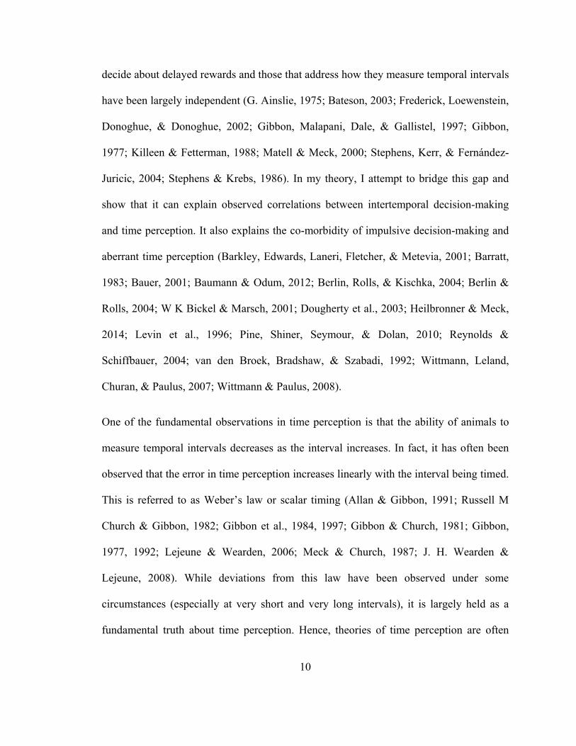
Figure 10 Analysis related to Figure 9
A-C. Quantification of shift in wait times induced by the presentation of laser (see 2.7.6).
A is reproduced from Figure 9B. My aim was to quantify the consistent shift observed
throughout the CDF, across different percentiles. To this end, I measured the shift

43
between the two distributions at each percentile and quantified the median percentile
shift, as shown in B. C. The null distribution of the normalized median percentile shift
(normalized by the interquartile range of the wait time distribution in no-laser trials) was
obtained using bootstrapping by resampling with replacement from the wait time
distribution of no-laser trials. The p value of the observed median percentile shift for this
session was calculated using a two-tailed measure (p<0.001). D-K. Single unit
recordings from one animal performed to confirm perturbations of neural activity indeed
showed that the laser (blue bar) affected neural activity across all intensities used.

44
2.5 Results: Spiking neuronal model & Reward responses
Based on these data, one can infer that V1 is involved in engendering action timing. But
what is the mechanism that gives rise to visually-cued action timing? Previous
experimental work has shown that the average delay between predictive cues and reward
(i.e. reward timing) can be locally generated within V1 (Chubykin et al., 2013). Further, a
computational model has been proposed for how such visually-cued temporal intervals
may be learned and expressed (Gavornik & Shouval, 2011; Gavornik et al., 2009).
Therefore, I and our collaborators (Marco Huertas and Harel Z Shouval) postulated that
action timing may arise from reward timing activity. To explore this possibility, we
examined whether the same local recurrent connections in V1 that give rise to reward
timing activity can also generate action timing. We reasoned that since a population of
neurons can report an average temporal interval (reward timing), a subpopulation could
be used to instruct the timing of an action, thereby expressing both reward and action
timing activity in V1. If so, would individual neurons in this subpopulation show trial-by-
trial correlations with the action despite the fact that only their aggregate activity instructs
the action? To address these questions, we modified our previous model of visually-cued
reward timing in V1 (Gavornik et al., 2009) (Figure 11A), so generating both action and
reward timing responses (see 2.7.7 for details). Individual neurons of the subpopulation
that reports the expiry of the interval and drives the action showed responses remarkably
similar to the experimental data, exhibiting significant trial-by-trial correlations with the
action (p<0.01, n=60 trials, bootstrapping) (Figure 11B). The remaining neurons

45
reflected only the average time between stimulus and reward, and not the individual
actions (Figure 12). Therefore, action timing can be derived from reward timing activity.

46
Figure 11 Spiking neuronal model
A. Schematic of the model showing the network architecture (“a” is the subpopulation
driving the action; see 2.7.7). B. Raster plot showing significant trial-by-trial correlations
with action, of example intervalkeeper (E population; p<0.001) and decoder (P
population; p=0.010) units. Each trial began 500 ms prior to visual stimulation. C. The
effect of the introduction of a “laser” perturbation in the model is shown using a CDF
plot and is quantified using its normalized median percentile shift (see 2.7.7). The
resultant significant shift in wait times (p=0.039, bootstrapping) is similar to the
population data shown in Figure 9D. Error bar is the s.e.m, as obtained using
bootstrapping. This result holds for a range of parameters in the model (Figure 12H).

47
Figure 12 Analysis related to Figure 11

48
A-C. The activity of each unit in the P population of the spiking neuronal network model
(as shown in Figure 11A) is shown for three different trials, showing action generation
(purple line) following visual stimulation (green bar) (see 2.7.7). The neurons controlling
the action are shown in purple. D-F. The summed population activity is shown for both
the action generating subpopulation (purple) and all others (black). The action is
generated at the peak of this summed activity, but even individual units show trial-by-
trial correlations with the action (as shown in Figure 11B). Importantly, the population
activity of the other neurons does not correlate with the action time, but reflects the
median reward time. G. The activity of single units that do not control the action does not
show trial-by-trial correlations with the action. Instead, these neurons represent the
median reward time. Neuron 156 is shown in upper panel and neuron 146 in the lower.
H. The range of normalized median percentile shifts observed for the model is similar to
the experimentally observed shifts across different parameters. For the experiments, the
shifts from all 18 sessions are shown. For the model, the fraction of excitatory and
inhibitory neurons activated by the laser in ascending order of observed shifts are: (10%,
20%), (5%, 10%), (8%, 10%), (9%, 20%), (10%, 10%), (6%, 10%) and (4%, 10%). I.
Individual sessions in both the experiment and the model show non-significant
differences in coefficient of variation due to the optogenetic perturbation (p>0.05 with
Holm-Bonferroni correction for multiple comparisons, two-tailed bootstrapping). The
population of shifts in CV is also not significantly different from zero for either the
experimental data (p=0.85, two-tailed Wilcoxon signed-rank test, W18=81, z = -0.1960)
or the model (p=0.19, two-tailed Wilcoxon signed-rank test, W7=3).

49

50
To test whether the above model (producing timed actions based on local recurrent
connections within a network) also explains the results of my optogenetic experiment, we
introduced a perturbation in the network mimicking the optogenetic perturbation (see
2.7.7). In order to assess whether the experimental observations can be sufficiently
explained by our model, we tested the following four questions: 1) does the perturbation
produce a shift in the distribution of wait times, 2) if so, is this a consistent shift in the
distribution, 3) is the magnitude of shift comparable to the experimental data, and, 4)
does the shifted distribution still abide by scalar timing? The answer to each question was
in the affirmative, as experimentally observed (Figure 11C and Figure 12). This confirms
that the experimentally observed shift in behavior is as expected if V1, as proposed in our
model, is instructing the timing of the action.
In order for the model to learn to predict and drive the timing of future actions, it would
need to receive a feedback signal that reflects the magnitude of reward received
(Gavornik et al., 2009) (see 2.7.7). Such primary reward responses have been reported in
auditory cortex (Brosch et al., 2011; FitzGerald, Friston, & Dolan, 2013) and
somatosensory cortex (Pleger et al., 2009; Pleger, Blankenburg, Ruff, Driver, & Dolan,
2008), but have not hitherto been reported within V1 (Weil et al., 2010). Because of the
unique design of my task in which different wait times lead to differing magnitudes of
reward, we were able to test whether the magnitude of received reward is conveyed by
the firing pattern of neurons in V1. I found that 23 units (Figure 13) showed significant
differences between rewarded and unrewarded trials in addition to showing a significant
correlation with the amount of reward received (see Figure 14 for analysis). This

51
confirms that primary reward information reaches V1, potentially permitting the
relationship between actions and rewards to be learned locally.

52
Figure 13 Reward magnitude response observed in V1
A. Example unit showing a response indicating the receipt of reward of a given
magnitude (larger the wait time, larger the reward obtained). Blue curve shows smoothed
spike counts (during 200-300ms following first lick and reward; shown by the blue bar)
for individual trials. B. 23/363 units show reward magnitude coding.

53
Figure 14 Analysis related to Figure 13 (A-C) and to Figure 3-Figure 7(D)

54
A-C. Analysis for testing reward magnitude information in V1 for the example unit
shown in Figure 13A. A. The probability histogram of spike counts (normalized for
number of trials) shows a higher firing rate in rewarded trials. B. This difference is
quantified as an AuROC and tested for significance by generating a sampling distribution
using bootstrapping (see 2.7.5). C. If the above comparison shows a significant difference
(p<0.05) between rewarded and unrewarded trials, I tested whether the spike counts
actually reflect the magnitude of reward obtained. The grey line shows the unsmoothed
spike counts on a trial with a given obtained reward magnitude; the cyan line is the best
fit linear correlation. The unit is deemed as representing reward magnitude information
only if both of these tests are significant, and if the difference in spike counts between
rewarded and unrewarded trials does not result from the difference in lick density (see
2.7.5). D. Flow chart showing the analysis of neural data for timing (see 2.7.5). The
latencies with maximum and minimum signed firing rate change are detected. An ROC
analysis detects whether a linear classified can assert the firing rates as changing at that
latency. If the firing rate change is significant, it is tested to see whether it can be
explained by reward timing, i.e. firing profile representing an average interval from the
visual stimulus. If it cannot be explained by reward timing, the activity is analyzed on
non-visually-timed trials and false first licks. If the neuron’s activity cannot be explained
by the mere presence of an action, it is classified as action timing and if it can be
explained by the action alone, it is classified as action feedback.

55
2.6 Discussion
The production of the stereotyped timing behavior observed in my visually-cued timing
task requires that the brain sense the presence of a visual stimulus, generate the
stereotyped waiting interval, and then produce the lick. The traditional view of primary
sensory cortices would assume that V1 has a role only in sensing the stimulus. However,
I show that the cue evoked responses in V1 evolve from those that merely reflect the
presence of a stimulus to those consistent with driving the timing of delayed voluntary
actions. By parsing the effect of the timed interval from the action indicating the lapse of
that interval, I show that neurons in V1 correlate with the action only when it is visually-
timed, ruling out the alternative that the correlation is merely due to the presence of the
action. This is the first time that a neural signal generating a timed action by a persistent
modulation of firing during the wait interval until action has been observed anywhere in
the cortex (Buhusi & Meck, 2005; Buonomano & Laje, 2010; Johnson, Goel, &
Buonomano, 2010; Leon & Shadlen, 2003; Matell & Meck, 2000; Merchant et al., 2013).
Prior reports of timing typically show peak responding (Shuler & Bear, 2006), ramps in
activity (Buhusi & Meck, 2005; Leon & Shadlen, 2003), oscillations (Buhusi & Meck,
2005; Matell & Meck, 2004; Merchant et al., 2013) or network representations
(Buonomano & Laje, 2010; Johnson et al., 2010). Perturbing activity in V1 during the
interceding interval indicates that V1 neurons contribute to instructing the decision of
when to lick. Note, however, that I do not claim that the timing of visually-cued actions
in this task is exclusively controlled by V1, or that other regions do not play a role. It is

56
possible that V1 might only be one of many regions that simultaneously control the
action of the timed lick in this task. In such a network of multiple controllers, assessing
whether V1 has any contribution to the instruction of timing requires perturbing its
activity. My optogenetic experiment was thus designed only to perturb the activity, rather
than silence it, since intact timing behavior under silencing may simply mean that other
regions also instruct timing or compensate for the absence of activity in V1. Perturbing
(rather than silencing) activity in V1 to show a shift in timing behavior, however, directly
addresses whether V1 itself has any role in the timing of the actions. Nevertheless, our
spiking neuronal model confirms that such control of timed actions can be performed
locally within V1 by a recurrent network of neurons. In our model, a recurrent network of
neurons was sufficient to produce timed actions, neural responses showing correlation
with the timed action, and, shifts in timing due to brief perturbations of network activity.
Interestingly, due to the unique design of my task with a continuous gradient of reward
depending on the time waited by animals, I also found primary reward responses in V1,
confirming that it does indeed receive feedback regarding the outcome of recent actions.
My data demonstrate that “higher order” decisions such as when to perform an action can
be instructed even by primary sensory areas.
My work raises the question of why a primary sensory area might be involved in the
instruction of timed actions. Since successful execution of this behavioral task merely
requires the sensation of a visual stimulus and the generation of a temporal interval prior
to motor production, an area that has the ability to sense visual stimuli and produce
temporal intervals would be capable of solving the task. Because of the metabolic cost

57
incurred from using more neurons than strictly necessary to optimally perform a task, I
posit that it may be sufficient for a primary sensory area to control highly stereotyped
actions so as to efficiently balance the trade-off between redundancy of processing,
metabolic demands, and reward maximization (Bullmore & Sporns, 2012; Namboodiri,
Mihalas, Marton, & Hussain Shuler, 2014).
2.7 Experimental Procedures
2.7.1 Subjects Animal subjects were wild-type adult male Long-Evans rats with weights between 300-
400g and age between P60-100. All experimental procedures were approved by the
Institutional Animal Care and Use Committee. The animals were singly-housed in a
vivarium with a 12 hour light/dark cycle and the experiments were conducted during the
day (light cycle).
2.7.2 Behavioral Task Prior to behavioral training, goggle posts were mounted using dental cement on the skull
of animals under sterile surgical conditions. Following a recovery period of 7-10 days,
animals were water deprived but given ad-lib access to food. Animals began behavioral
training after two days of water deprivation. During this period, they obtained water only

58
within the behavioral task in addition to brief scheduled access periods every day and a
night of free access every week.
The behavioral task was a visually-cued timing task, performed in a standard operant
chamber (Med Associates) containing a port (nosepoke) that housed a lick tube. A
behavioral session consisted of 360 trials. A nosepoke entry was required to initiate a
trial. After the nosepoke, a random delay of 0.6-1.6s expired during which the animal is
allowed to lick. At the expiry of this random delay, if the animal had not licked in the
previous 0.2-1.2s (randomly set on each nosepoke entry), the visual stimulus was
presented to either the left or the right eye (Figure 1A). If instead the animal had licked,
0.2-1.2s had to elapse without a lick for the visual stimulus to be presented. The visual
stimulus was a full field green LED-powered flash of 100ms presented using detachable
head-mounted goggles covering each eye. Entries into the nosepoke and licks were
registered using two IR emitter-receiver pairs (Med Associates). If, without having exited
the nosepoke, the rat subsequently licked following the offset of the visual stimulus, it
immediately received a water reward with a probability of 5/6. Rewarded and
unrewarded trials were randomly interleaved such that no more than 4 unrewarded trials
could be presented in a row. The reward volume was chosen depending on the wait time
as shown in Figure 1B. The reward delivery system used a solenoid (custom modified to
eliminate any operational noise) which was controlled by a microcontroller generating
sub-millisecond precision for open times. A trial ended when the rat exited the nosepoke.
An obligatory intertrial interval (ITI) of 500ms was enforced after every trial such that
the animal had to wait outside the nosepoke until its expiry. Entries into the nosepoke

59
within the ITI did not result in a visual stimulus presentation and caused a reset of the
ITI. After every 12 trials, animals were presented with a “NoStim” trial (total of 30, in
addition to 360 visual stimulus presentations). In this trial type, the animal had to wait in
the nosepoke as it would on a visual stimulus trial but instead of a light flash, no stimulus
was presented. These NoStim trials were included so as to determine whether licking
behavior was driven by and timed from the visual stimulus, as well as to assess neural
activity on trials in which a lick was registered following this NoStim event. As
mentioned in the text, licks after a NoStim or false entry to the nosepoke (during the
mandatory ITI) were combined to form the “false first licks” as shown in Figure 5A,B
and Figure 6 and Figure 8. Early in training, the following behavioral shaping was used.
On the first day of training, the animals were given a free reward on every trial 500 ms
after the corresponding nosepoke entry. If the animals did not stay in the nosepoke until
visual stimulus presentation, no further free reward was delivered on the next nosepoke
entry. The lick-free pause (shown in Figure 1A) required to deliver a visual stimulus was
set between 200-400 ms. Free rewards were then subsequently delivered only on the first
200, 100 and 20 trials respectively in the next 3 sessions. On the 4th session, the lick-free
pause requirement was increased to 200-600 ms, followed consecutively by 200-800 ms,
200-1000 ms and finally, 200-1200 ms, as they progressed in training. This resulted in
the animals licking prior to visual stimulus presentation only on a very small fraction of
trials (<10%) by the final stage. In some cases, to speed the rate at which the animals
increased their wait time, the ramp duration (wait time at which maximum reward was

60
obtained) was increased to 2 seconds. Once the median wait time increased beyond 1s,
the ramp duration was held at 1.5 seconds.
2.7.3 Behavioral analysis All analysis in this chapter was performed by custom-written scripts in MATLAB (The
Mathworks). I did not do a power analysis for the sample sizes used as there are no
reasonable estimations for the expected distributions of the various statistics measured for
this study, as the phenomenology is novel.
When parsing non-visually-timed and visually-timed trials, any trial with a wait time less
than 300 ms and a wait time greater than 3000 ms was also grouped into the category of
non-visually-timed trials (I do not necessarily know if these were timed from the
nosepoke, but it is unlikely that they were timed from the visual stimulus, and since I was
only interested in testing visually-timed trials against non-visually timed trials, these were
included along with the non-visually-timed trials). Subsequently, the effect of removing
individual trials on the R2 of the correlation between the delay from nosepoke entry to
visual stimulus presentation and the wait time was measured (whenever the original
correlation was significant). If removal of a given trial produced a reduction in
correlation that was 1.5 times the interquartile range from the median change in
correlation, it was deemed to be a non-visually-timed trial (Figure 2).
For behavioral sessions early in training, there were some additional constraints placed
on the analysis. If the coefficient of variation of the wait time distribution was greater

61
than 0.6 (very low precision), it was deemed that the animal had not yet learned to time
its licks from the visual stimulus. This happened only early in training and neural
recordings were obtained from such sessions only in the three animals shown in Figure 7.
Nevertheless, the neural analysis as discussed below was carried out to test for trial-by-
trial correlations with the action, even though, at this early stage, I could not test whether
visually-timed and non-visually-timed trials showed different neural responses.
2.7.4 Neural recordings Once the animals were deemed behaviorally-trained (at least three consecutive sessions
with median wait times greater than one second), custom-built 16-channel electrode
arrays were implanted bilaterally in V1 (targeted stereotaxic coordinates of 1.5mm
anterior and 4.2 mm lateral to lambda at a depth of 1mm) following sterile surgical
procedures.
The electrode implant surgeries were performed once the animals learned the task (at
least three consecutive sessions with median wait times greater than a second), except for
three animals for which data was acquired early in training (Figure 7E). During the
surgery, animals were anesthetized using isoflurane, had scalps shaved, were given
dexamethasone (.2mg/mL), and were placed into a stereotaxic apparatus atop a heating
pad. After swabbing the area to be incised with betadine and ethanol, a subcutaneous
injection of lidocaine (0.1mL) was administered. An incision was made and connective

62
tissue was retracted to expose the skull. The surface of the skull was dried by applying
3% hydrogen peroxide, following which six screws were uniformly placed across the
exposed skull. Bilateral craniotomies and durotomies were then made overlying the
primary visual cortex to implant custom-made movable 16-channel electrode arrays.
Following the insertion of electrodes, the ground wires were wrapped around the screws,
and a petrochemical gel was applied on the exposed surface of the brain. The entire skull
was then covered with dental cement. The animal was given a subcutaneous drug cocktail
containing an antibiotic (gentamicin, 1mg/mL) and an NSAID (flunixin, 4mg/mL).
The same parameters were used for recovery and subsequent water deprivation prior to
recordings during behavior. Experiments were continued only in the animals (n=5) that
produced usable neural recordings. No blinding or randomization of subjects was
performed as these experiments used a within-subject design.
The electrode arrays were moved down by a distance of approximately 15-60 µm on a
day, if necessary, so as to increase the yield of single unit recordings. Signal from each
electrode array was sent to headstage amplifiers, and, bandpass filtered (1-10 kHz) neural
signals were sampled at 33 kHz by commercially available hardware (Neuralynx).
Commercially available software packages were used to manually sort the waveforms
into single units (Offline Sorter, Plexon) and to visualize the timestamps (Neuroexplorer,
Nex Technologies) of these sorted units. The manual sorting was done by tracing the
boundaries of the clusters in a 3D space formed by three of the following variables:
principal components 1 and 2, valley timing, non-linear energy and peak minus valley
amplitude. Units with unstable waveforms or greater than 3% refractory period (1.5 ms)

63
violations were excluded, along with multi-unit recordings. A unit was deemed as
different from any previous recording if one of the following criteria were met: 1) no unit
was observed from the same channel on the previous session; units recorded from the
same channel on the previous day showed 2) different waveforms, or 3) different
visually-evoked response; or, 4) the electrode array was moved more than 60 µm
between the two sessions. If none were met, then the unit was deemed as a repeat. In this
case, only the first instance was counted.
For obtaining histological confirmation of electrode locations, animals were deeply
anesthetized with pentobarbital and transcardially perfused with 1x PBS followed by 4%
PFA. Brains were then harvested and stored in 4% PFA until being transferred to a
solution of 30% sucrose in PBS until time of sectioning. Brains were sectioned into 60µm
slices and mounted on gelatin-coated slides (FisherBrand). Slices were then imaged using
an inverted microscope (Zeiss Instruments). Electrode tracks were verified to be found in
V1 (see Figure 4D).
2.7.5 Analysis of neural response To test whether there were any trial-by-trial correlations between the activity of a single
unit and the first lick, I tested whether there was a significant change in firing rate locked
to the first lick in visually-timed trials, separately for left-eye-stimulated and right-eye-
stimulated trials. To this end, I checked whether a linear classifier could decode the firing
rate change between a 100 ms bin before and after a given latency from the first lick. The
latencies tested were -300 ms, -250 ms, -200 ms,…, 100 ms, and, 150 ms. I restricted the

64
decoder analysis to only the two latencies that led to the maximum and minimum signed
change in firing rate. Since I was testing only these two bins for significance, I corrected
for multiple comparisons using Bonferroni correction. Trials with less than 1 Hz of firing
in a window starting from 200 ms prior to the visual stimulus to 200 ms after the first lick
were excluded.
Once the latencies with maximum and minimum firing rate changes were identified, units
that fired less than 1 Hz in both of these bins were excluded from further analysis.
Further, only trials in which the visual stimulus turned off at least 100 ms prior to each
latency were included in the analysis for that latency. To test whether an ideal observer
can measure the change in firing rate at a given latency, I quantified the area under an
ROC curve (AuROC) formed by the spike count distributions for the 100 ms bins
flanking the latency. Another possible method was to test whether the peri-stimulus time
histogram showed a significant increase in firing rate locked to the first lick. In order to
test significance, most standard methods assume Poisson statistics of firing. However, the
units recorded in my task often violated this assumption (data not shown). Further, I was
interested in quantifying whether a downstream decoding area could tell the difference in
firing rate so as to instruct the action. For this purpose, a linear decoding strategy such as
that assumed in ROC analysis was deemed more appropriate. Additionally, I was also
interested in testing whether the change in firing rate was consistently present across
trials. This was implicitly tested by my resampling method (explained below) in which I
resampled individual trials, as opposed to individual spike counts.

65
Next, I asked two questions to ascertain whether there is a firing rate change locked to the
action of the first lick (Figure 14D). First, I asked whether there was a statistically
significant change in firing rate from that expected by chance. Second, I asked whether
this change could be completely explained by visually-evoked activity. The latter was
required to rule out changes locked to the action that did not truly result in or from the
action. The significance testing for AuROC was done by estimating the sampling
distribution using bootstrapping (Figure 14D). This was done by sampling with
replacement 18000 (= number of latencies tested×2000; so p=0 implies p<0.001 after
Bonferroni correction) times from the available pool of trials, i.e. individual trials were
resampled, including both the earlier and later bin. The p value was tested by reading off
the percentile at which chance level of 0.5 for the AuROC lay, using a two-tailed test
(Obuchowski & Lieber, 1998). If this p value was found to be less than 0.05, it means
that there was a significant change in firing rate at the corresponding latency. Further
action-timing analysis was performed only if this was true. The next step, as mentioned
above, was to test whether the observed change in firing rate could be explained by
visually-evoked activity. This was done by generating fake first lick events (not to be
confused with false first licks) for each trial, by randomly permuting the wait times. This
ensured that the mean interval between the visual stimulus and the fake first lick is
preserved, but the relationship to individual trials, being shuffled, was randomized. If
such shuffling did not affect the AuROC at the corresponding latency with respect to the
new fake first licks, then the change in firing rate was judged to have resulted from
visually-evoked activity, and not timing of, or execution of, the action. Such a procedure
was repeated 18000 times to generate the sampling distribution of AuROCobserved -

66
AuROCfakefirstlicks. The p value was read off as the percentile at which chance level of zero
lay. If this p value was also found to be less than 0.05, the neuron was deemed to show
trial-by-trial correlations with the action (“action unit”).
The next step in the action timing analysis was to determine whether the trial-by-trial
correlations between the neural activity and the action could be explained by the mere
presence of the action, or whether it required the trial to actually be timed from the visual
stimulus. To this end, I tested whether the change in firing rate observed at the given
latency was present also on non-visually-timed trials and false first licks. This was done
by conducting a two-sample version of the significance test mentioned above
(Obuchowski & Lieber, 1998) to generate sampling distributions of AuROCvisually-timed-
AuROCnon-visually-timed and AuROCvisually-timed-AuROCfalsefirstlicks, and determining the
corresponding p values (labeled p1 and p2). An example is shown in Figure 6. Further, to
test whether there were any significant trial-by-trial correlations of the activity with non-
visually-timed licks and false first licks, I repeated the same analysis that was performed
on visually-timed trials, i.e. it was tested whether there was any significant change in
firing rate at the given latency on non-visually-timed licks (labeled p3) and whether the
observed firing rate change was explained by the visually-evoked activity (labeled p4). It
was also tested to see whether there was a significant change in firing rate at the given
latency with respect to the false first licks (labeled p5).
The animals from which the neural recordings early in training were obtained were
implanted prior to any behavioral training and were also run on a reward profile that
ramped to 1 second instead of 1.5 seconds. The lowest coefficient of variation of the wait

67
times from a session with at least one single unit recorded was 0.45 across these animals,
showing that the recordings were all made in an early stage of learning. Early in training,
the earliest latency tested for trial-by-trial correlations with the action depended on the
wait time distribution (this was true also for neurons later in training, but the following
procedure later in training always resulted in the earliest latency being -300 ms). This
was done to avoid the short-latency visually-evoked activity from directly affecting
action responses. If the 25th percentile of the wait time distribution was greater than 500
ms, the earliest latency tested was -300 ms from the action. Instead, if it fell between 400
and 500 ms, the earliest latency tested was -200 ms, and if it was between 300 and 400
ms, the earliest latency tested was -100 ms and if it was between 200 and 300 ms, the
earliest latency tested was 0 ms. If the 25th percentile fell between 100 and 200 ms, the
earliest latency tested was 100 ms with respect to the action and if it was less than 100
ms, the units from that session were not analyzed for action timing.
The neural report of time for a unit was defined as the earliest latency at which it
contained any information about the action (in either left-eye or right-eye visually-timed
trials). Based on the p values obtained for the five comparisons (p1-p5) mentioned above,
the unit was subsequently classified as “action timing” or “action feedback”, or as “action
timing/feedback” if this classification could not definitively be made (owing to low
number of non-visually-timed and false first licks). Action timing units were those that
showed both p1 and p2 lower than 0.05, i.e. visually-timed licks were different from both
non-visually-timed and false first licks. Action feedback units were those that were not
action timing, but rather showed a significant change in firing rate locked either to non-

68
visually-timed licks (p3<0.05 and p4<0.05) or false first licks (p5<0.05). All remaining
units were classified as “action timing/feedback”.
A significant (p<0.05) eye difference for the action timing response on action
timing/feedback units (Figure 7D) was tested by checking whether the AuROC for the
action response was different following the stimulation of both eyes. This difference
(|AuROClefteye–AuROCrighteye|) is labeled as “eye-specificity index” in Figure 7D.
To classify units as intervalkeepers or decoders, action units (showing trial-by-trial
correlations with the action) were manually classified using the following criteria: if the
unit showed a sustained response from visual stimulus to action, it was called an
intervalkeeper. If instead, it only showed a peak modulation around the action, it was
called a decoder. If it showed both, it was called an intervalkeeper and a decoder.
For the reward timing analysis shown in Figure 4B, the following analysis was
performed. In order to test whether the firing rate showed any long-latency modulations, I
compared long-latency responses evoked by the stimulation of either eye to the baseline
firing rate observed just prior to the stimulus presentation. A window of 100 ms was used
to obtain the baseline spike counts. The activity in the first 300 ms following visual
stimulus onset was considered as a transient response, and hence, was not analyzed. I
used a sliding window of 100 ms, sliding by 50 ms, up to a maximum of 2 seconds, to
test for significant modulations of firing with respect to baseline, using an ROC analysis
(quantified by AuROC). Significance testing was done using bootstrapping, similar to the
action timing analysis. The longest streak of consecutive significant modulation was
identified, and if this streak lasted less than 300 ms, the unit was deemed as a non-reward

69
timing unit. Instead, if the unit showed significant modulation in more than 6 consecutive
bins (spanning 300 ms), the unit was deemed as a reward timing unit. In order to
determine the neural report of time, the firing profile was first classified as a sustained
excited, sustained inhibited or a peak excited or peak inhibited profile. If the longest
streak of modulation did not begin for at least 500 ms after the visual stimulus offset, the
response was classified as a peak; otherwise, it was classified as a sustained response.
The sign of the modulation determined whether it was excited or inhibited. For sustained
responses, the neural report of time was defined as the last bin that showed significant
modulation compared to the baseline, whereas for peaks, it was defined as the bin
showing maximum modulation. The reward timing index for a unit was defined as the
ratio of the difference between the neural response of time and the median wait time to
the sum of these two quantities. For instance, if the neural report of time was 1.22
seconds for a session with median wait time equaling one second, the reward timing
index will be ~0.1. This is the median reward timing observed for the population, as
shown in Figure 4B.
For analyzing primary reward responses in V1 as shown in Figure 13, the following
analysis was performed. Reward responses were quantified by testing the spike count
distribution of one of three possible bins, all starting 200 ms after the action (reward
onset) and ending at one of 300, 400 or 500 ms. All p values were corrected for multiple
comparisons using Bonferroni correction. For each bin, the spike count distribution on
rewarded trials was tested against that on unrewarded trials using AuROC. If this was
found to be significant, the response was subsequently tested to determine if there was a

70
significant correlation between the spike counts on a trial and the reward obtained. The
neuron was deemed to convey reward magnitude information only if both the above tests
were significant. Further, I also tested whether the observed difference between rewarded
and unrewarded trials resulted from a difference in licking behavior for these trial types
in the corresponding bins. To this end, I quantified the lick count and spike count on each
trial and tested whether the change in spike counts between rewarded and unrewarded
trials was linearly correlated with the corresponding change in lick counts. This was done
using bootstrapping by resampling with replacement from the available trials and
generating a sampling distribution of the slope in linear correlation. If the sampling
distribution was significantly different from zero, it was deemed that the difference in
neural activity between rewarded and unrewarded trials resulted from the difference in
lick rates on the corresponding trials. No unit tested showed such a relationship (p>0.5).
2.7.6 Optogenetics Animals were injected with either the virus containing the channelrhodopsin (ChR2)
construct (UPenn Vector Core: AAV9.CAG.ChR2-Venus.W.SV40 (Petreanu, Mao,
Sternson, & Svoboda, 2009)) or saline randomly, using sterile surgical procedures as
described below. The investigator was not blind to the identity of each animal; however
all analyses were fully automated.
Three craniotomies were made overlying primary visual cortex (V1; 1-2mm anterior, 4-
4.5mm lateral from Lambda) in order to allow for cortical infections at two depths (0.9-
1.0mm and 0.5mm ventral from dura). A nanoliter injector (Drummond Scientific) was

71
backfilled with mineral oil as well as either the virus containing the channelrhodopsin
(ChR2) construct (UPenn Vector Core: AAV9.CAG.ChR2-Venus.W.SV4049) or saline.
The injector was then lowered into the most ventral depth and KwikCast (World
Precision Instruments) was applied to the surrounding area and allowed to cure before
infusing. The pump introduced 32.2nL of infusant every 10s over 2.5 minutes for a total
volume of 483nL after which the tip was kept in place for 5 minutes to ensure that all
infusant diffused away from the tip. The injector was then raised to the more dorsal
infection site and another injection was similarly carried out. This process was repeated
for each craniotomy for a total of 12 infections delivering roughly 5.8µL of infusant
throughout cortex. Following infusions, Kwikcast was placed atop each hemisphere’s
three craniotomies, and, after curing, the skin was sutured together.
After at least a month, animals underwent a second surgery in which optical fibers were
placed at the surface of the brain bilaterally (1.5mm anterior and 4.2mm lateral to
lambda) along with goggle posts. In one experimental animal infected with ChR2,
custom-built bundles of sixteen electrodes were also implanted bilaterally at a depth of
1.0mm at the above mentioned coordinates, so as to verify that the optogenetic
perturbation indeed affected neural activity (Figure 10D-K).
For obtaining immunohistochemistry to confirm ChR2 infection, animals were perfused
and brains sectioned as described above. After sectioning, using a mini-orbital shaker,
slices were washed in 1x PBS for ten minutes three times before being blocked in
10%NDS/0.5%triton-X/PBS solution for one hour. Slices were then incubated with a
primary anti-GFP antibody (ab290, abcam) overnight at 4C. After three 10m 1xPBS

72
washes, slices were incubated with the secondary donkey anti-rabbit 488 antibody (Alexa
Fluor) to verify protein expression (see Figure 9D).
Prior to optogenetic testing, the dental cement headcap of each animal was painted black
using nail polish so as to prevent the leakage of laser light. The laser was a 473nm blue
light (Cobolt, Blues 473nm DPSS laser).
For this experiment, the ramping profile of the reward was offset by 500ms (no reward
for wait times less than 500ms; done to ensure that the bulk of first-licks fell after the
laser offset), reaching the same maximum reward volume at 1500ms. There was a 50%
probability that a given trial would result in a laser presentation lasting 200ms (300ms
after visual stimulus offset). The laser and no-laser trials were computer-generated and
randomly interleaved throughout a session of 360 trials. Laser was also presented on 50%
of the NoStim trials to test whether the laser was treated as a visual stimulus, thereby
triggering licking behavior. In each of the experimental animals (n=3), two sessions each
were run at laser intensities of 0.21, 0.69 and 1.67 mW/mm2 (measured at the tip of the
optical fiber that is placed on the surface of the brain), thereby producing 18 data points.
In one of the saline control animals (n=4), only the highest intensity was used since one
implanted optical fiber failed prior to testing the lower intensities, and in another, one last
session at 0.21 mW/mm2 could not be performed for the same reason. This resulted in a
total of 19 (6+6+2+5) data points from the saline group.
One possible way to quantify whether the optogenetic perturbation caused any significant
change in wait time is to do a Kolmogorov-Smirnov test to check for significant
differences in distributions of wait times between laser and no-laser trials. However, my

73
aim was to test whether there was a consistent shift introduced by the presence of the
laser, rather than merely testing for differences in distribution (for instance, KS test also
returns significance for significant change in variance). To this end, I defined the shift
statistic as the absolute median percentile shift (see below) and generated bootstrapped
sampling distributions for significance testing. This is also why I avoided standard
ordinal tests that simply check for differences in median.
The absolute median percentile shift was calculated thus: for the CDF of wait times, for
each percentile (i.e. 0, 1, 2, …., 99, 100 percentile), the shift in wait times between the
“laser” and “no laser” trials was measured. The absolute value of the median of this list
of one hundred data points (i.e. shifts at each percentile) was defined as the absolute
median percentile shift (see Figure 10).
There were three different statistical tests performed on this dataset, corresponding to
three different questions. In all cases, only first licks following the laser offset were
analyzed. The first question was whether, in an individual session, laser trials had a
significant shift in wait times.
To this end, the observed median percentile shift was compared against that expected by
chance. The null distribution was created by resampling with replacement from the wait
time distribution in no-laser trials and measuring the absolute median percentile shift for
each resampling. This was repeated 2000 times to calculate a two-tailed p value for the
observed median percentile shift. This resulted in 8 statistically significant shifts in the
experimental group out of a total of 18 sessions, along with 3 sessions with a p value

74
between 0.05 and 0.06. There were no significant shifts (at p>0.05) observed in the 19
sessions of the control group.
The second test was to determine whether the population of all observed absolute median
percentile shifts was significantly different from that expected by chance. As my aim was
only to test whether there was an observed shift for the group as a whole (and not to
quantify the shift for each individual laser intensity), I pooled the data from all sessions.
Since the larger the variability in the wait times, the larger the shift expected by chance
will be, the absolute median percentile shifts were normalized for each animal by
dividing it by the inter-quartile range of the wait time distribution in no-laser trials. To
test whether the population of normalized absolute median percentile shifts (n=18) was
significantly different from that expected by chance, it was compared against the
bootstrapped null distributions generated from the 18 individual sessions (using the
procedure mentioned above after normalization) and was significant in all cases
(p<0.001, one-tailed). For the purpose of Figure 9, the null distribution of one randomly
selected session was used.
The above two questions only answer whether the laser presentation led to an observable
shift in the wait time distribution in experimental animals. However, this observed shift
could be the result of non-specific effects of laser presentation. To test against this
possibility, I tested the population of normalized absolute median percentile shifts from
the experimental animals (infected with ChR2) against the saline-control animals. Since I
could not assume homoscedascity for these two populations, I performed the Welch’s t

75
test for the hypothesis that the shift in the experimental group is larger than the shift in
the control group.
In order to test whether the significant effect of the laser in the aggregate as shown in
Figure 9C was consistently present in all animals, I tested individual experimental
animals against the controls. Even under greatly reduced statistical power, I found that
two animals showed significant differences with the control group (p values of 0.01 and
0.03) with the remaining animal missing significance (p=0.11, one tailed, Welch’s t test).
In this last animal, three individual sessions showed significant shifts in wait time
distribution between laser and no-laser trials. In order to test whether the optogenetic
results were significant merely due to the duplication of data at each laser power, I also
tested the difference between the experimental and saline groups after averaging the
observed shifts at each intensity within an animal. The comparison is still significant
(p=0.0061, one-tailed, t=2.92, Welch’s t test).
To test whether the laser presentation led to an observable increase in the probability of
licking in individual experimental animals, I tested for differences in the probability of
licking in the presence and absence of laser using bootstrapping with 10,000 re-samples
with replacement. To correct for the multiple comparisons, I used Holm-Bonferroni
correction (since it is more powerful than Bonferroni correction) and found no significant
effect in any animal (p>0.05).

76
2.7.7 Spiking neuronal model The model (uploaded to ModelDB and available upon request) consisted of three
populations of spiking neurons forming a network as illustrated in Figure 11A. Two
populations, labeled E and P, contain excitatory neurons and the other, labeled I, is
formed by inhibitory neurons. All synaptic weights are denoted by the form Wij, where
the indices i and j label post- and pre-synaptic populations. The magnitudes of these
weights were learned as explained previously (Gavornik & Shouval, 2011; Gavornik et
al., 2009) so as to represent a median interval of one second. Recurrent synaptic
connections within E (WEE) and P (WPP) populations and projections between these
(WPE) had a spatial probability of connection that is Gaussian-distributed with a standard
deviation equivalent to 12 neighboring neurons, while connections between excitatory
and inhibitory populations (WIE, WEI, WIP, WPI) were sparse with a uniform 20%
probability of connection.
Neurons in each population were modeled as leaky integrate-and-fire units. The equation
for the membrane potential for neuron i is described by the differential equation
( ) ( ) ( ), , L L i E i E i I i I idVCdt
g E V g E V g E V= − + − + − (2.1)
where C is the membrane capacitance, Vi is the membrane potential; gL, gE,i and gI,i are
the conductance of the leak current, total excitatory and total inhibitory synaptic currents,
respectively, and EL, EE and EI are the corresponding reversal potential of each current.

77
To simulate the effect of optogenetic activation of neurons, we included an additional
current of the form IChR2 = gChR2,i (EChR2-Vi), where gChR2,i and EChR2 are the conductance
and reversal potential of the membrane current associated with ChR2.
Except for the leak conductance, the total synaptic conductance takes the form (e.g. for
excitation) gE,i = gE Σ Wij sj, where gE is the maximum conductance of the current, sj is
the synaptic efficacy of presynaptic synapse j and Wij is the synaptic strength. Each sj is
modeled as an exponentially decaying function that obeys the differential equation
( ) ( ) 1k kk pre
s
ds s s t tdt t
ρ δ= − + − −∑ (2.2)
where τs is the synaptic decay time constant, ρ is the fractional change in synaptic
efficacy due to the arrival of a presynaptic spike that occurs at time tpre and the sum is
over all pre-synaptic spikes; δ is the Dirac delta function.
We computed the response of the network to an initial presentation of a 100 ms long full-
field visual stimulation, represented as a train of action potentials with a constant firing
rate. The initial values of the synaptic weights WEE, WPP and WPE were obtained after
training (Gavornik & Shouval, 2011; Gavornik et al., 2009) so that the activity of the
excitatory population E exhibited an initial rise in its firing rate in response to the visual
stimulation followed by a slow decay due to reverberations within the population that
decayed to baseline 1000 ms after the stimulus on average. Changes in synaptic weights
were calculated using the Reward-Dependent Expression (RDE) rule (Gavornik et al.,

78
2009). The output from the E population, and consequently from the I population onto P,
led to a response that was qualitatively similar to the previously observed peak responses.
Once trained, the values of these synaptic weights remained constant for the rest of the
simulations.
To simulate the spontaneous activity of neurons, all three populations received feed-
forward excitatory input in the form of random Poisson distributed spike trains at a
constant frequency of 5 Hz. The addition of noise induced trial-by-trial variability in the
response of the network. Furthermore, to represent a transient visual input, excitatory
populations E and P received additional excitatory feed-forward input at a higher mean
rate, representing drive from the visual thalamus. In this network, the E population
represents “intervalkeepers” since they represent the target interval in the duration of
sustained responses triggered by the visual stimulus. The P population represents
“decoders” since they represent the moment of target interval expiry. Action neurons
were selected from the P population and consisted of 10 neurons that were spatially close
in synaptic connectivity, and thus showed a high degree of correlation. The action was
signaled when the summed firing rate of this subpopulation exceeded 15 Hz and reached
its peak value (Figure 12). Other neurons in this population, synaptically distant from
these action neurons, were thus less correlated to the action neurons and (consequently)
the time of action. Hence, they did not represent the action time, but represented the
median reward time (Figure 12).

79
For simulating the optogenetic perturbation, we modeled the activation as affecting more
inhibitory neurons than excitatory ones. This was for two reasons. First, based on the
firing patterns of the neurons recorded during optogenetic stimulation, the predominant
effect in the network is the inhibition of activity, as is observed immediately following
laser offset (Figure 10D-K). Second, the laser power decreases rapidly over depth of the
cortex and hence, the strongest activation would be in the superficial layers. In layer 1,
~90% neurons are inhibitory(Fitzpatrick, Lund, Schmechel, & Towles, 1987; Hendry,
Schwark, & Jones, 1987; Meinecke & Peters, 1987). Within the excitatory populations (E
and P), we assumed an equal split of neurons getting activated. The identity of the
neurons getting activated within each subpopulation was randomized. We found that if
inhibitory activation was twice that of excitatory activation, the network was nearly
balanced with the resulting shift in wait times being minimal. For the simulations in
Figure 11C, 9% of the excitatory neurons and 20% of the inhibitory neurons were
activated for 200 trials. The activation ratios were systematically varied, showing
perturbations similar to those observed experimentally (Figure 12).

80
Chapter 3. Rationalizing decision-making: understanding the cost and perception of time
3.1 Introduction
The question of how animals, including humans, make decisions between differently
sized rewards at differing delays (“intertemporal decision-making”) has been the subject
of at least eight decades of active research, in fields as diverse as economics, psychology,
evolutionary ecology, neuroscience and addiction. Across the spectrum of these fields,
researchers have approached this problem in myriad ways, with some proposing theories
of animal behavior and others measuring animal behavior experimentally. However, there
has not yet been significant agreement between theories and experiments. In this chapter,
I review theoretical work addressing this problem, in the context of some recent advances
in experiments and my own theoretical contributions.
In order to make decisions about delayed rewards, animals must be able to measure those
delays. Hence, the problem of “intertemporal decision-making” is intertwined with time
perception. However, theoretical and experimental work on 1) how animals measure
delays, and, 2) how they make decisions between differently delayed rewards, has been
largely non-overlapping. Nevertheless, there has been some recent work, both theoretical
and experimental, that examines the connection between how animals make
intertemporal decisions and how they perceive time. In the latter half of the chapter, I

81
therefore focus on time perception, in the context of recent experimental attempts and my
theoretical contributions to create a unified understanding of intertemporal decision-
making and time perception.
First, I will provide a historical account of theories of intertemporal decision-making.
3.1.1 History of theories of intertemporal decision-
making
The problem of intertemporal choice was first mentioned in 1834 by John Rae (Rae,
1834). In his work, he wondered about the origins of differences in wealth between
nations. Rae claimed that one of the key determinants of wealth of a nation is the nation’s
“desire of accumulation”. The desire of accumulation, according to him, was determined
by the balance between two kinds of psychological factors, one that motivates the nation
to invest and save for the future and another that derives pleasure from immediate
consumption. Thus, the idea of making decisions about delayed outcomes was framed as
the conflict between two different psychological impulses of humans (and societies).
The notion of intertemporal choices being driven by innate psychological quantities stuck
ever since John Rae and persists to this day (Warren K Bickel et al., 2007; Frederick et
al., 2002; Kalenscher & Pennartz, 2008; Madden & Bickel, 2010; McClure, Laibson,
Loewenstein, & Cohen, 2004; van den Bos & McClure, 2013). The first attempt to
mathematically formalize the treatment of such psychological factors was made a century
82
later by Paul Samuelson in 1937 (Samuelson, 1937) (but see (Bohm-Bawerk, 1889;
Fisher, 1930)) when he invented the “Discounted Utility Theory” (DUT). It is important
to point out that DUT was borne out of ideas that originated from John Rae, and thus
shared many of the same limitations. For instance, both models framed decisions as being
based on a purely subjective quantity representing self control, rather than any objective
maximization of fitness (will be discussed later). Nevertheless, it was the first simple and
mathematically tractable formulation of the problem of intertemporal choice. Briefly,
DUT states that intertemporal choices are made so as to maximize the “net discounted
utility” of the future. Here, DUT assumes that the “utility” of a reward is given by its face
value, if it were to be received immediately. For instance, the utility of $20 is $20,
irrespective of when you receive it. However, the immediate subjective value of $20
delayed by a fixed amount would be given by its “discounted utility”.
The key postulate of DUT is that the “discounted utility” of a delayed reward is
determined by an exponential discounting function, with the exponential constant—the
discount rate—determining the ability of a person to delay gratification. In simpler terms,
the discount rate measures the patience of an individual—the lower the discount rate, the
higher your patience in waiting for a reward, i.e. the longer you are willing to wait to
obtain that reward. The major simplification achieved by Samuelson was in compressing
the different psychological factors of John Rae and others into a single, measurable
parameter of self-control.

83
The other major advance made by Samuelson was in treating the utility of different future
rewards as the sum of their respective discounted utilities. This “net discounted utility”,
as mentioned earlier, was expressed as shown below.
0
Maximize ( ) ( ) ; where ( )T
ktU D t u t dt D t e−= =∫ (3.1)
Here, D(t) is the discounting function, and u(t) is the utility of a single reward received at
a delay of t. Time was assumed to be integrated up to a maximum delay of consideration,
also known as the temporal horizon of a decision, represented by T.
Samuelson’s model was simple and elegant, with its exponential form particularly
attractive, owing to similarities with the calculation of compound interest. It further
provided a single, measurable parameter of an individual’s ability to delay gratification
(viz. k). Despite all these advantages, however, Samuelson had a number of reservations
about the validity and utility of his model. Since most of these concerns were ignored by
future researchers due to its distinct advantages, I would like to point them out here, in
Samuelson’s own words.
Concern 1 (pp. 159 Samuelson, 1937): “In the first place, it is completely arbitrary to
assume that the individual behaves so as to maximize an integral of the form envisaged.
This involves the assumption that at every instant of time the individual's satisfaction
depends only upon the consumption at that time, and that, furthermore, the individual
tries to maximize the sum of instantaneous satisfactions reduced to some comparable
base by time discount.”

84
Concern 2 (pp. 160 Samuelson, 1937): “A less important point to be noted is the fact that
our equations hold only for an individual who is deciding at the beginning of the period
how he will allocate his expenditures over the period. Actually, however, as the
individual moves along in time there is a sort of perspective phenomenon in that his view
of the future in relation to his instantaneous time position remains invariant, rather than
his evaluation of any particular year (e.g. I940). This relativity effect is expressed in the
behavior of men who make irrevocable trusts, in the taking out of life insurance as a
compulsory savings measure, etc….Moreover, in the analysis of the supply of savings, it
is extremely doubtful whether we can learn much from considering such an economic
man, whose tastes remain unchanged, who seeks to maximize some functional of
consumption alone, in a perfect world, where all things are certain and synchronized.”
In sum, Samuelson wrote “any connection between utility as discussed here and any
welfare concept is disavowed”, stressing that there was no a priori reason why his model
would be a valid or normative way of describing human behavior.
Despite these strong reservations, Samuelson’s work paved the way for the exponential
model of discounting, and more generally, the idea of discounting functions, to be
ingrained into work on intertemporal choices (Benzion, Rapoport, Yagil, Science, & Mar,
1989; Fehr, 2002; Fishburn & Rubinstein, 1982; Frederick et al., 2002; Kalenscher &
Pennartz, 2008; Laibson, 1997; Lancaster, 1963; Madden & Bickel, 2010; Thaler, 1981;
van den Bos & McClure, 2013). DUT received further theoretical support in 1960 when
Koopmans showed that DUT can be derived from a set of simple axioms (Koopmans,
1960). The most important axiom was the statement (one that Samuelson recognized, as

85
mentioned above) that the intertemporal preferences of an individual are stationary over
time, i.e. if an individual prefers option 1 in a choice between option 1 and option 2, if the
delay between the two options is fixed, the individual will always prefer option 1,
independent of how much time has elapsed since the first decision was made. Like
Samuelson, Koopmans also did not argue for the normative or descriptive validity of
these axioms.
Nevertheless, further work on intertemporal choice in economics considered consistent
time preferences and stationarity as a fundamental tenet of human rationality (see
Drouhin, 2009; Fishburn & Rubinstein, 1982; Frederick et al., 2002; Koopmans, 1960;
Lapied & Renault, 2012a, 2012b; Strotz, 1956 for discussion). However, experimental
evidence repeatedly showed that this core postulate is violated by humans (G. Ainslie &
Monterosso, 2003; G. Ainslie, 1975; Benzion et al., 1989; Frederick et al., 2002; Green,
Fristoe, & Myerson, 1994; Holt, Green, & Myerson, 2003; G. Loewenstein & Prelec,
1992; McClure et al., 2004; Thaler, 1981), pigeons (G. W. Ainslie, 1974; Chung &
Herrnstein, 1967; Rachlin, Green, & Vi, 1972) and rats (Bennett, 2002; Ito & Asaki,
1982). In fact, the axiom of constant time preference can be immediately seen to be
violated by considering the following two example choices: “which would you prefer:
$100 now or $105 in a month?” and “which would you prefer: $100 in a year or $105 in a
year and one month?” It should be immediately clear that while most people prefer $105
in the second question, they prefer $100 in the first, thus violating the assumption of
stationary preferences.

86
In the face of such overwhelming evidence, there are two possible recourses to solving
the apparent contradiction: 1) change one’s definition of rationality, or, 2) state that all
the animals tested above are irrational. Many economists chose the latter option,
maintaining the axiom of stationary time preferences (and exponential discounting) as
“rational” (see Drouhin, 2009; Lapied & Renault, 2012a, 2012b for a discussion). This is
partly due to equating stationarity and time consistency (see Drouhin, 2009; Lapied &
Renault, 2012a, 2012b for a discussion), and partly due to the fact that other models of
rationality, like reward rate maximization(Bateson & Kacelnik, 1996; Stephens &
Anderson, 2001; Stephens & Krebs, 1986; Stephens, 2008), have not been successful in
explaining animal behavior.
In addition to the violation of the assumption of stationarity of choices, many other
assumptions of DUT have been shown to be violated by human behavior. For instance,
DUT assumes consumption independence—the utility of a reward does not depend on
whether or not that reward was obtained in the immediate past. This is patently false, as
surely animals can become sated over time. Consider too, for instance, that the preference
for a restaurant will obviously depend on whether or not an individual ate there for the
past five days. There are numerous other violations of DUT that are not going to be
discussed here. For a more detailed overview of these violations, see prior reviews on this
topic(Frederick et al., 2002; Kalenscher & Pennartz, 2008).
An assumption related to the stationarity axiom is that the discount factor (rate of
discounting per unit discounting) is constant over time. Behavioral scientists and
psychologists have shown that this, too, is repeatedly violated in experiments across

87
many different species (G. Ainslie & Monterosso, 2003; G. W. Ainslie, 1974; G. Ainslie,
1975; Benzion et al., 1989; Calvert, Green, & Myerson, 2010; Green et al., 1994; Holt et
al., 2003; Kobayashi & Schultz, 2008; Rachlin et al., 1972; Thaler, 1981). In fact, it was
observed experimentally in 1967 that delayed food rewards were preferred in inverse
proportion to their delay (Chung & Herrnstein, 1967). This relationship was later
mathematically reformulated within the framework of a discounting function by Ainslie
(G. Ainslie, 1975) and experimentally confirmed by numerous subsequent papers (e.g. G.
Ainslie & Monterosso, 2003; G. W. Ainslie, 1974; G. Ainslie, 1975; Benzion et al., 1989;
Calvert et al., 2010; Green et al., 1994; Holt et al., 2003; Kobayashi & Schultz, 2008;
Rachlin et al., 1972; Thaler, 1981). Specifically, this discounting function, that
approximated intertemporal choice behavior better than exponential discounting
functions, was hyperbolic in form. The animal’s choice under this conception can be
expressed mathematically as shown below:
1 max( ( ) ( )); ( )1
Choose r t D t D tkt
=+
(3.2)
where D(t) represents the discounting function, r(t) is the reward magnitude of a reward
available at delay t and k is the discounting constant.
It is important to point out that the casting of experimental observations into a
“discounting function” framework is due to the legacy of Samuelson’s work(Samuelson,
1937). In this view, the agency for the reduction in value of a reward with delay
(temporal discounting) is due completely to a psychologically-innate discounting
function. The contribution of Ainslie provided a much better descriptive model of

88
experimental data. However, the contribution was only to find that a hyperbolic
discounting function provided a better fit to experimental data than an exponential
discounting function, and not a rationale for why hyperbolic discounting would better
describe the data.
Recently, many other forms of discounting functions have been proposed that provide
even better fits to experimental data than pure hyperbolic discounting functions (al-
Nowaihi & Dhami, 2008; Green & Myerson, 2004; Killeen, 2009; Laibson, 1997;
McClure et al., 2004; Schweighofer et al., 2006; van den Bos & McClure, 2013). Among
the most prominent are quasi-hyperbolic discounting functions (Laibson, 1997) and β-δ
discounting functions (McClure et al., 2004; van den Bos & McClure, 2013).
A major limitation of the hunt for the perfect discounting function to fit experimental data
is that it provides only that—a fit to the data. It does not provide an explanation for why
animals discount delayed rewards the way they do. Further, it also cannot rationalize the
observed steepness of temporal discounting (a measure of patience, like k in DUT) of an
individual in a given reward environment. Hence, all the different discounting functions
described above are fits to the data which are assumed to originate from some innate
psychological quality. For instance, finding that β-δ discounting functions provide better
fits to experimental data has been used to infer that the brain has two separate systems
involved in processing immediate and delayed rewards, respectively. Indeed, recent
human imaging studies have shown that different areas of the brain are differentially
involved when a subject is considering an immediate or a delayed reward (McClure et al.,
2004) (see Kalenscher & Pennartz, 2008; van den Bos & McClure, 2013 for reviews).

89
A wholly different perspective to the problem of intertemporal choice, not wed to the
notion of a discounting function, can be obtained by considering the field of behavioral
ecology. In 1966, a highly influential paper was published in theoretical behavioral
ecology by MacArthur and Pianka (MacArthur & Pianka, 1966). This paper considered
how foraging animals should decide between different patches of food, if they behaved
economically. It introduced the idea that animals should forage so as to maximize their
net energy intake in the long run. Net energy intake was operationally defined as the total
reward obtained per unit time spent in obtaining it. The idea behind the postulate was
simple: obtaining a maximal rate of food intake would maximize the chances of living.
Hence, in this conception, time was not merely a component of decision-making, but the
most important dimension over which rewards needed to be accumulated.
The idea of maximizing long-term reward rates was the key thesis behind many
subsequent theories on optimal foraging (Charnov, 1976a, 1976b; B. Y. J. R. Krebs,
Erichsen, & Webber, 1977; J. R. Krebs, 1978; Pyke, Pulliam, & Charnov, 1977; Pyke,
1984). This literature is too vast to be fully considered here. For a detailed review of such
theories, see (Pyke, 1984; Stephens & Krebs, 1986). Together, these theories came to be
known as the Optimal Foraging Theory (OFT).
Mathematically, OFT’s postulate of maximizing long-term reward rates can be expressed
as:
1
1
i
i
ii
rMaximize
t
∞
=∞
=
∑
∑ (3.3)
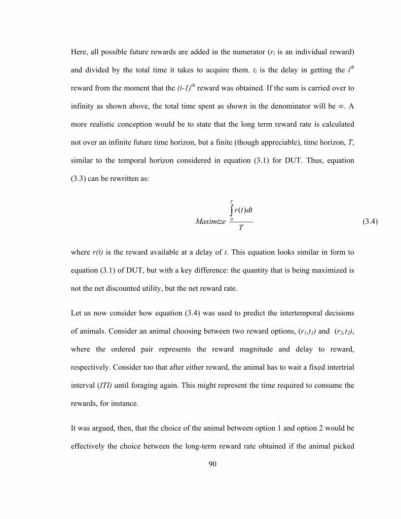
90
Here, all possible future rewards are added in the numerator (ri is an individual reward)
and divided by the total time it takes to acquire them. ti is the delay in getting the ith
reward from the moment that the (i-1)th reward was obtained. If the sum is carried over to
infinity as shown above, the total time spent as shown in the denominator will be ∞. A
more realistic conception would be to state that the long term reward rate is calculated
not over an infinite future time horizon, but a finite (though appreciable), time horizon, T,
similar to the temporal horizon considered in equation (3.1) for DUT. Thus, equation
(3.3) can be rewritten as:
0
( )
T
r t dtMaximize
T
∫ (3.4)
where r(t) is the reward available at a delay of t. This equation looks similar in form to
equation (3.1) of DUT, but with a key difference: the quantity that is being maximized is
not the net discounted utility, but the net reward rate.
Let us now consider how equation (3.4) was used to predict the intertemporal decisions
of animals. Consider an animal choosing between two reward options, (r1,t1) and (r2,t2),
where the ordered pair represents the reward magnitude and delay to reward,
respectively. Consider too that after either reward, the animal has to wait a fixed intertrial
interval (ITI) until foraging again. This might represent the time required to consume the
rewards, for instance.
It was argued, then, that the choice of the animal between option 1 and option 2 would be
effectively the choice between the long-term reward rate obtained if the animal picked

91
option 1 alone, and, the long-term reward rate obtained if the animal picked option 2
alone. Thus, the animal’s choice could be written as
max( ) ; i {1,2}i
i
rChooseITI t
∈+
(3.5)
Here, the total reward rate achieved if the animal picked only option i is the reward
magnitude of option i divided by the total effective time spent per receipt of reward.
Interestingly, a closer examination of equation (3.5), along with equation (3.2) reveals
that the choice of maximizing reward rate as expressed in (3.5) is similar to maximizing a
hyperbolically-discounted reward, with the hyperbolic constant k (Equation (3.5))
replaced by 1/ITI. Thus, it was argued that maximizing long-term reward rate underlies
the experimentally observed hyperbolic discounting function mentioned earlier. This was
the first instance wherein the agency for the decay in value of delayed rewards was not
placed on an innate discounting function, but on the need to maximize an ecologically-
relevant metric of fitness, i.e. reward rate.
Especially in the context of foraging, maximizing fitness or reward rate was a better
definition of “rational” decision-making than stationarity of time preferences. However, it
was soon obvious that while the experimental data on intertemporal decisions indicated a
hyperbolic discounting function, this function did not result from a maximization of
reward rates as considered in OFT. This was because, in experiments in which animals
were given choices between two reward options but where the total trial duration was a
constant (and not the ITI), animals did not always pick the larger reward (G. W. Ainslie,
1974; Bateson & Kacelnik, 1996; Blanchard, Pearson, & Hayden, 2013; Cardinal,

92
Pennicott, Sugathapala, Robbins, & Everitt, 2001; Grossbard & Mazur, 1986; Alex
Kacelnik & Bateson, 1996; Kalenscher et al., 2005; Kobayashi & Schultz, 2008; Louie &
Glimcher, 2010; James E Mazur, 1988; Pearson, Hayden, & Platt, 2010; Rachlin et al.,
1972; Roesch, Calu, & Schoenbaum, 2007; Stephens & Anderson, 2001; Winstanley,
Theobald, Cardinal, & Robbins, 2004). This was a direct challenge to the choice
algorithm shown in equation (3.5) since the effective time spent on either option was
equal, but the animals still did not pick the option with the larger reward magnitude.
In the face of apparent empirical rejection, behavioral ecologists proposed an alternative
decision-making algorithm within the realm of rate maximization. It was proposed that
instead of maximizing long-term reward rates, animals maximized single-trial reward
rates (Bateson & Kacelnik, 1996; Real, 1991; Stephens et al., 2004; Stephens & Krebs,
1986; Stephens, 2008). This approach has been referred to by many different names
across the literature (Bateson & Kacelnik, 1996; Real, 1991; Stephens et al., 2004;
Stephens & Krebs, 1986; Stephens, 2008), but I will refer to it by the name of Ecological
Rationality Theory (ERT), as used by (Stephens et al., 2004; Stephens, 2008). Regardless
of the name, however, all these papers propose the following choice algorithm:
max( )i
i
rChooset
(3.6)
The major difference between the predictions of equations (3.5) and (3.6) is in the
inclusion/exclusion of the various delay components into the decision. While equation
(3.5) (OFT) considers all effective intervals within a trial, ERT only considers the delay
to reward. Post-reward delays of any sort are excluded in the decision algorithm of ERT.

93
The rationale for their exclusion was that in the wild, foraging animals rarely decide
between options with differing post-reward delays associated with them. In fact, it was
argued (Stephens et al., 2004; Stephens, 2008) that typical decisions in the wild are not
even in the form of binary choices as presented above. Instead, it was argued (Stephens et
al., 2004; Stephens, 2008), that typical decisions in the wild have a “foreground-
background nature”, i.e. that a choice is presented always in the context of background
activity. Interestingly, it was shown that in laboratory tasks where such a foreground-
background structure was presented to animals, equation (3.6) resulted in long-term
reward rate maximization, as expressed in equation (3.4) (Stephens & Anderson, 2001;
Stephens, 2008). This result—that in typical foraging decisions, maximizing single-trial
reward rates is the same as maximizing long-term reward rates—provided support for the
argument that animals only maximized single-trial reward rates, and is the basis of the
name, Ecological Rationality Theory.
While ERT provided better fits to experimental data in the foraging literature than OFT
(Bateson & Kacelnik, 1996; Stephens & Anderson, 2001; Stephens, 2008), it was
nevertheless insufficient at providing quantitative fits to the experimental data collected
in standard psychological tasks involving binary choices. This was because the effective
discounting constant predicted by equation (3.6), according to a hyperbolic discounting
function, is ∞. Yet, every discounting study measured finite, non-zero discounting
constants (G. W. Ainslie, 1974; Bateson & Kacelnik, 1996; Blanchard et al., 2013;
Cardinal et al., 2001; Grossbard & Mazur, 1986; Alex Kacelnik & Bateson, 1996;
Kalenscher et al., 2005; Kobayashi & Schultz, 2008; Louie & Glimcher, 2010; James E

94
Mazur, 1988; Pearson et al., 2010; Rachlin et al., 1972; Roesch et al., 2007; Stephens &
Anderson, 2001; Winstanley et al., 2004).
In conclusion, theories from behavioral ecology that attempted to rationalize
intertemporal decision-making within the framework of reward-rate maximization failed
to provide satisfactory explanations for empirical data. Further, the theory (DUT) based
on the assumption that temporal discounting must lead to stationary time preferences, and
hence should abide by exponential discounting, is also inconsistent with experimental
observations. Only psychological models like the hyperbolic discounting model proposed
by Ainslie (G. W. Ainslie, 1974; G. Ainslie, 1975), among others (al-Nowaihi & Dhami,
2008; Green & Myerson, 2004; Killeen, 2009; Laibson, 1997; McClure et al., 2004;
Schweighofer et al., 2006; van den Bos & McClure, 2013), provided good fits to
observed data from laboratory tasks. These models, however, are not based on any
normative principle of decision-making, unlike DUT, OFT and ERT, and therefore do not
rationalize why apparent discounting functions take the shape that they do.
3.2 Recent experimental and theoretical advances in the
study of intertemporal decision-making
In this section, I will focus on recent advances in aligning theories and experiments of
intertemporal decision-making. For this purpose, I only consider normative theories and

95
models that propose principles of intertemporal decision-making. For recent descriptive
models that attempt to fit data, see the literature (al-Nowaihi & Dhami, 2008; Killeen,
2009; van den Bos & McClure, 2013).
3.2.1 Experimental advances
As was mentioned in Section 1.1, the crucial observation that invalidated the idea of
long-term reward rate maximization was the finding that animals do not include post-
reward delays in their decisions (G. W. Ainslie, 1974; Bateson & Kacelnik, 1996;
Blanchard et al., 2013; Cardinal et al., 2001; Grossbard & Mazur, 1986; Alex Kacelnik &
Bateson, 1996; Kalenscher et al., 2005; Kobayashi & Schultz, 2008; Louie & Glimcher,
2010; James E Mazur, 1988; Pearson et al., 2010; Rachlin et al., 1972; Roesch et al.,
2007; Stephens & Anderson, 2001; Winstanley et al., 2004). This meant that in a choice
between two rewards that effectively take the same time, the animals did not necessarily
choose the larger reward, hence violating the idea of reward rate maximization. It was
also found that delays common to both options, like the ITI term in Equation (3.5) did not
have an effect that matched that expected from maximizing long-term reward rates
(Bateson & Kacelnik, 1996; Logue, Smith, & Rachlin, 1985; J E Mazur, 2001; James E
Mazur, 1989; Snyderman, 1987; Stephens & Anderson, 2001).
While these observations were a severe challenge to the idea of long-term reward rate
maximization, some researchers realized that it was not a death blow (Blanchard et al.,
2013; Alex Kacelnik & Bateson, 1996; Stephens, 2002). An explanation for these
96
observed results could be that animals are not able to learn the association between the
rewards and their corresponding post-reward delays. Were they able to learn the
association between a post-reward delay and the choices presented, they could potentially
have chosen the larger option, consistent with reward rate maximization. Hence, it is not
that animals do not maximize reward rates; it is just that they do so within constraints of
evolved mechanisms of associative learning. This idea was first presented in 1996 by
Alex Kacelnik and Melissa Bateson (Alex Kacelnik & Bateson, 1996). They proposed the
following mechanistic explanation for why delays following the receipt of reward might
not be learned by animals performing standard intertemporal decision-making tasks.
In order to measure the preferences of animals between two delayed rewards, they are
first trained to learn the meaning of two conditioned stimuli (CS) (usually visual or
auditory cues) that correspond to either reward option. In other words, prior to receiving
the choices, the animals are presented with the CSs and their associated delayed rewards
and post-reward delays. Once the animals learn the meaning of both CSs, they are
presented with choice trials in which they should pick one or the other CS, so as to
receive the corresponding delayed reward. In order to learn the association between a CS
and the corresponding reward, it was argued that it makes functional sense for the
learning to be driven by the receipt of reward, so as to learn the causal relationship
between the CS and the reward (Dickinson, 1980; Alex Kacelnik & Bateson, 1996). In
this framework, the retrospective assignment of value to the CS is driven only by the
reward and not the moment of expiry of the post-reward delay. Hence, it was argued that
the reason for choice behavior being insensitive to post-reward delays was simply due to
97
the lack of its learning. For a similar mechanistic argument from reinforcement-theory,
based on neural recordings from honeybees, see (Montague, Dayan, Person, &
Sejnowski, 1995).
An indirect support to the above hypothesis was provided in 2010 when Pearson et. al.
found that presenting explicit cues to indicate the lapse of a post-reward delay made the
choice behavior of monkeys move towards long-term reward rate maximization (Pearson
et al., 2010). Specifically, they designed the CSs to be vertical bars whose length was
proportional to the net delay associated with that choice. The moment of receipt of
reward was indicated by a colored horizontal line placed at a location corresponding to
the delay to reward. The color of the reward line represented the reward magnitude.
Hence, the post-reward delays were indicated by the length of the bar following the
reward line. Crucially, as the monkeys chose an option, the other option disappeared from
the screen and the chosen option’s vertical bar started to shrink in proportion to the
passage of time. In this way, the monkeys were explicitly cued to the passage of the delay
to reward and the post-reward delay. Interestingly, the explicit cueing was sufficient to
increase the monkeys’ choice for the larger reward, thus indicating that in the presence of
explicit information of the post-reward delays, the choice behavior of monkeys accorded
better with long-term reward rate maximization.

98
Figure 15. Modified from Figure 3 of (Blanchard et al., 2013)
Behavior of 3 monkeys is shown in a task that compares their performance between a
standard intertemporal decision-making task (“std”) in which post-reward delays are
adjusted to make the trial duration constant, and a random variant of the task in which the
post-reward delays are randomly chosen for each option (“rand”). As can be seen, all
three monkeys showed similar discounting steepness across the standard and random
variant, indicating that they did not appropriately learn the relationship between the
rewards and their corresponding post-reward delays. The optimal performance of an
agent that correctly learns this relationship is shown by the black bar (“opt”), showing
that none of the monkeys are optimal.

99
Nevertheless, a direct test of the above-mentioned hypothesis would have been to test
whether animals performing intertemporal choices can associate the appropriate post-
reward delay with a given option. This is exactly what Blanchard et. al. did in 2013
(Blanchard et al., 2013). In their study, they performed three variants of the experiment
mentioned above, but without any explicit cueing of the post-reward delay. In other
words, in all their three experiments, the vertical bars only indicated the delay to reward.
In the first experiment, they compared the performance of monkeys in the standard
intertemporal choice task (with post-reward delays adjusted to have constant trial
duration) to their performance in a task where the post-reward delays were randomly
shuffled between the options. If the monkeys were able to correctly associate the post-
reward delays with their corresponding reward, their performance would be different
across these two versions. However, their results clearly indicated that monkeys failed to
associate the post-reward delays to their corresponding reward option (Figure 15).
Since the above hypothesis claims that learning is only triggered by the receipt of reward,
another prediction is that when the post-reward delays are followed by a reward, they
should be included in the decision. Blanchard et. al. confirmed this prediction in a second
experiment by presenting a small, but equal volume of reward at the end of the post-
reward delays of both options. This, too, increased the likelihood of the monkeys
choosing the larger reward.
Finally, in the third experiment, they addressed whether the monkeys’ preferences were
sensitive to the magnitude of the post-reward delay. In this experiment, they used an
equal post-reward delay for both reward options, much like a constant ITI in earlier

100
experiments, and varied it from 0s to 10s. Their results showed a clear dependence of the
discounting steepness on the duration of the post-reward delay. This is similar to the
effect of the ITI term in Equation (3.5), except that the parameter that fit the choice data
was always significantly lower than the real delay used. The reason for this discrepancy
was claimed by the authors to result from a biased measure of the post-reward delay by
the monkeys. However, it must be pointed out that prior tasks studying the effect of
intertrial intervals did not observe as clear a dependence of the discounting constant on
the ITI (Bateson & Kacelnik, 1996; Logue et al., 1985; J E Mazur, 2001; James E Mazur,
1989; Snyderman, 1987; Stephens & Anderson, 2001). Further, in many timing tasks,
animals’ perception of time is much more accurate than is required for these results to be
explained by biased time perception, i.e. animals represent intervals at least up to ten
seconds quite accurately (e.g. Buhusi & Meck, 2005; Matell & Meck, 2004). Thus, it is
likely that the reason for this discrepancy might not result fully from an inaccurate
perception of post-reward delays. For a more detailed discussion of this point, see Section
2.2.
In sum, the experiments of Blanchard et. al. (Blanchard et al., 2013) convincingly
demonstrate that the reason for insensitivity of choice behavior to post-reward delays is
the lack of ability of animals to correctly associate those delays with the corresponding
reward option. Hence, it would be incorrect to rule out theories of long-term reward rate
maximization purely on the basis of this observation. In the next section, I present a novel
theory of intertemporal decision-making which is based on reward rate maximization. I
present the theory from first principles.

101
3.2.2 Theoretical advances
Were decision-making simply the evaluation of offered reward magnitudes, the learning
of the relationship between cues and their associated reward amounts would suffice to
understand choice behavior. However, if offers are differentially displaced in time, the
simple determination of which cue connotes the greatest reward no longer suffices to
understand choice behavior should the goal of an animal be to gather the most reward
while in an environment. The reason, as previously mentioned, is that time itself has a
cost; in having chosen to pursue a larger later reward over a smaller earlier reward, the
difference in reward amount achieved must outstrip the difference in the time invested
which could otherwise be put to use in further gainful activity.
In the prior sections, I reviewed theories that contend with this issue. One such theory,
DUT, is based on the normative argument that intertemporal decisions must be stationary
in time, which, as mentioned, does not hold up to experimental scrutiny. And why, if
mechanisms of intertemporal decision-making evolved under pressures of foraging,
would stationary preferences be a better normative argument than simply the
maximization of reward rates? From an evolutionary perspective, theories based on
reward rate maximization (Stephens & Anderson, 2001; Stephens et al., 2004; Stephens
& Krebs, 1986) are more compelling, yet also do not well explain experimental data as
animals do not include post-reward delays in their decision-making. Nevertheless, the
exclusion of post-reward delays does not in itself rule out rate maximization as the goal,
as it has been shown that their disregard is a consequence of an inability to learn the
experimental contingency (Blanchard et al., 2013). Hence, my goal here is to approach

102
the problem from the point of view of reward rate maximization, as in OFT. However,
whereas OFT only considers future options inferred from the current choice as affecting
decision-making, I show that it is the past that matters to estimate the cost of time so as to
maximize long-term reward rates.
To appreciate this difference in approach, let us start with the stated goal of OFT—to
maximize long-term reward rates. As one cannot change the decisions made in the past,
what is wrong with the seemingly reasonable notion in OFT that decision-making to
maximize reward rate would be concerned only with the future, being wholly prospective
in its outlook? An obvious constraint on so seeking to maximize long-term reward is
that, in most decisions, one cannot know the future pattern of rewards beyond those
currently available. But for the sake of argument, let us ignore this constraint and
consider the case wherein an animal (or an agent) can see many choices (or trials) into the
future. Specifically, let us consider an agent that can see ten future trials with each
requiring a choice between different reward options. In order to achieve the stated goal
of OFT, the agent will now have to calculate the optimal choice path across all ten trials.
There is only one method to obtain the exact optimal solution: the agent will have to
consider all 210 possibilities to determine the option-path that leads to the highest reward
rate. In other words, on choice number 1, the agent will have to consider the effect of that
choice on all possible future choices, and so forth. Clearly, such an exact solution is
computationally intensive, with the combinatorial explosion making it infeasible for an
animal to perform this computation beyond some limited number of trials.
103
Therefore, given that the exact solution is not attainable, how could one arrive at an
approximate solution? Maximizing reward rate requires an animal to not waste time on a
given trial, if that given trial presents options that are significantly worse than the
environment as a whole. Hence, at its core, it requires the animal to be able to compare
the reward rate available on a trial with the reward rate available on the session as a
whole, so as to make an appropriate decision on that trial. A solution is to estimate the
average reward rate of the ten known trials so as to estimate the reward rate achievable in
the session as a whole. However, this is only possible under the assumption that the
future is knowable. Therefore, let us now revoke this unrealistic assumption.
If the environment is assumed to be stationary (time-independent statistics), an
approximate solution can yet be to use the past as a model to predict the immediate
future, as the correlation between the immediate past and the immediate future is likely
high. Of course this approximation would work only if the environment is stationary in
time. Let us call such an epoch of time, modeled by the animal to be stationary, as a
“session”. An example is a typical experimental session in the laboratory with
unchanging reward statistics. Hence, a simple approximate solution to maximize reward
rates over the session can be to maximize the reward rates over the time that one has
spent in the session, i.e. instead of maximizing the reward rate prospectively in the
session, maximize the reward rate achieved in the session so far. This solution contrasts
with the solution presented by OFT shown in equation (3.5) because equation (3.5)
assumed that the net reward rate for a given option is the reward rate achievable if one
chose only that option. Instead, we use the past to compare the worth of a given option to
104
the environment as a whole. This is the rationale for my theory, named Training-
Integrated Maximized Estimation of Reinforcement Rate (TIMERR). In the remainder of
this section, I formalize the above argument and show the implications it has on choice
behavior.

105
Figure 16. Does the past matter?
A) Maximizing reward rate on a trial basis. An agent (black circle) presented with offers
of reward that vary in magnitude and temporal displacement ((r1, t1) or (r2, t2)) may
decide upon a given option by calculating which offer yields the highest rate of reward in
the trial. By normalizing reward magnitudes by the times to their future acquisition,
Option 1 (red vector) in the instance given is found to have the highest trial reward rate.
Trial reward rate is depicted graphically as the slope of the vector connecting the agent in
the present moment (now) along the x-axis of time to the magnitude of future reward. B)
Maximizing session reward rate. Alternatively, an agent presented with the same offers of
reward as that in (A) may decide upon a given offer by calculating which option yields
the highest session, rather than trial-rate of reward. Session reward rate is depicted
graphically as the slope of the line connecting the agent on entry into the environment—
its “past” self (grey circle) along the x-axis of time—to the magnitude of future reward.
By normalizing the magnitude of a reward offered by the sum of the time already spent in

106
the session plus the time to its future acquisition, Option 2 (blue vector) is found to have
the highest session reward rate. C) Comparing choice behavior governed by trial reward
rate versus session reward rate. By comparing the choices made by the agents in A and B
to the same reward offers, it is apparent that decision-making governed by trial and
session rate maximization are not equivalent, as they can lead to opposite choice
behavior. Hence, if the objective is to gather the most reward while within a given
environment, the past does in fact matter, as even evidenced when only considering
elapsed time in the environment.

107
Figure 17. The effect of “looking-back” different amounts of time in evaluating
realizable session reward rates
A) No “look-back” time. Should a session-reward-rate-maximizing agent look into its
past no amount time (as potentially the case were it to have just entered into a foraging
environment) it would choose Option 1 in the depicted example, as it yields the highest
session reward rate. In this special case where Time = 0, evaluating reward options by
maximizing session reward rate is equivalent to maximizing trial reward rate. B)
Increasing Time (while decreasing the realizable session reward rates) does not affect the
option chosen until Time reaches a value, as depicted in (B), wherein the reward options
affect equivalent session reward rates. In this case, option 2 would be chosen as
frequently as option 1. Growing the time in which the agent looks back into its past
beyond this point results in a reversal of choice from Option 1 to Option 2, as depicted in

108
(C). Therefore, the setting of Time critically affects the evaluation of delayed reward
offers.

109
3.2.2.1 The past matters
An agent, as in Figure 16, presented with offers of reward that vary in magnitude and
temporal displacement ((r1, t1) or (r2, t2)), may decide upon a given option by calculating
which offer yields the highest rate of reward in the trial. By normalizing reward
magnitudes by the times to their future acquisition, Option 1 (red bar) in this instance is
found to have the highest trial reward rate. Trial reward rate is depicted graphically as
the slope of the choice vector connecting the agent in the present moment (“now”) along
the x-axis of time, to the magnitude of future reward (the slope of the red and blue
vectors). Alternatively, an agent presented with the same offers of reward may decide
upon a given offer by calculating which option yields the highest session, rather than trial
rate of reward. Session reward rate is depicted graphically as the slope of the line
connecting the agent on entry into the environment, its “past” self (grey circle) along the
x-axis of time, to the magnitude of future reward. By normalizing the magnitude of a
reward offered by the sum of the time already spent in the session plus the time to its
future acquisition, Option 2 (blue bar) is found to have the highest session reward rate
(slope of the blue vector). By comparing the choices made by the agents in A and B to
the same reward offers, it is apparent that decision-making governed by trial and session
rate maximization are not equivalent, as they can lead to opposite choice behavior.
Hence, if the objective is to gather the most reward while within a given environment, the
past does in fact matter, as even evidenced when only considering elapsed time in the
environment.

110
Hence, what it means to select a reward option that “maximizes the rate of reward”
depends, as evidenced in the prior figure, on the objective of the agent. An agent that
makes its current choice based on maximizing the session reward rate—by considering
how much time it has already spent in the environment—will outperform an agent that is
wholly prospective (without including a model of the future based on the past) in its
decision-making. Therefore, as a commonly stated goal within optimal foraging is to
gather the most reward while within an environment, the former of the two agents would
rightly be regarded as the rational of the two.
If wholly prospective decision-making is not characteristic of rational decision-making, is
exhibiting a consistency in choice behavior to the same reward options (like in DUT)?
Consider an agent (as depicted in Figure 17) that maximizes the session rate of reward.
When being presented reward options upon entering an environment, as in panel A, the
session-rate-maximizing agent selects option 1. However, if a quantity of time were to
have passed in the environment prior to the presentation of the same reward options, as
depicted in panel B, at that moment, choosing either option would be regarded as
equivalent. Indeed, were even more time to have passed in the environment prior to
presentation of the same options (as in panel C), option 2 would be selected. In all cases,
the reward options presented are the same, making choice behavior appear to be
inconsistent across the same reward offers. Only from the perspective of selecting the
option that results in the highest session reward rate can choice behavior be regarded as
actually being consistent, resulting in different reward options being selected.

111
3.2.2.2 TIMERR Algorithm
Till now, I have considered the effect of the past on the valuation of reward offers under
the special case that the agent has not acquired any (net) reward over that time. Of
course, an agent may acquire reward in its past, and, should it have done so, the amount
consumed need be taken into account in its current decision-making. Why is this so? In
the prior figure, I provide an explanation as to why “looking back” in time would and
should affect intertemporal decision-making even when the agent has not, to the present
moment, accumulated any net reward. The benefit of looking back into one’s recent
experience can be appreciated in another way, however, apart from simply the time spent
in an environment, by considering, in addition, that a notion of experienced reward rate
can be determined by normalizing the accumulated rewards harvested by the time spent
harvesting in the environment. Therefore, one looks into the past not only to appreciate
what interval reward rate should be maximized over, but to apprehend the rate of reward
as already experienced in the environment.
Consider the case where the experienced environment has been a net positive one,
meaning that the sum of acquired rewards (denoted by R) over the “look-back” time
(Time) has a positive value. Whatever the rate of reward experienced over this past look-
back interval, offers of future reward must yield a rate greater than the experienced
reward rate to ensure that the reward rate of the session increases. Therefore, looking
back serves the purpose of determining the rate of reward that one should expect of an
environment: reward options that decrease the experienced rate of return signify that
they are subpar options that should not be taken.

112
The rate of experienced reward can be incorporated into the graphical depiction as
previously given for the (special) case—wherein the rewards accumulated in the
environment sum to zero, as in Figure 17—to yield a depiction of the decision-making
algorithm in the general case where accumulated reward can take on any value, be it
positive or negative (Figure 18). As in Figure 17, the right hand y-axis in Figure 18 plots
the magnitude of future reward offers. Also as in Figure 17 (though there not labeled as
such), the left hand y-axis plots the magnitude of accumulated past reward, the value of
which the backwardly pointing grey vector terminates. Whereas in Figure 17, the
backward pointing grey vector points to a value of accumulated past reward equal to
zero, in Figure 18 it points to some positive value of accumulated past reward, R, thereby
shifting the origin of the left-hand y-axis representing accumulated past reward
downward. The rate of experienced reward (R/Time) is thus graphically depicted as the
slope of the line connecting the agent’s past self with its current self (black vector). By
depicting accumulated past rewards and future reward offers in this manner, the
relationship between the past reward rate and the offered future reward rates can be seen
to sum to yield the realizable session reward rates (the slope of the red and blue vectors).
Given known reward offers, deciding between offers is then simply a matter of
determining which opportunity yields the highest session reward rate, and, should it
exceed the experienced reward rate, choosing that reward option. Expressed another way,
offered reward rates are added to the experienced reward rates to determine session
reward rates, the largest of which (so long as it exceeds that which is already
experienced) is then selected. This can be expressed as the following choice algorithm:

113
max( )ime
r RChooset T++
(3.7)

114
Figure 18. The TIMERR decision making algorithm and its graphical depiction
The TIMERR algorithm can be understood simply as choosing the option that leads to the
highest reward rate over the experienced interval within an environment up to and
including the time to the future reward option. Reward accumulated within the
environment (R) over the time the agent looks back into its past (Time) yields the
experienced reward rate (R/Time, slope of the black vector) which is added to the reward
rate of a future option (ri, ti) to yield a realizable reward rate having chosen that option.
The agent then selects the realizable reward rate with the highest rate of return. A caveat
is that the agent may forgo an option even if it evaluates to the highest realizable reward
rate should that rate be less than the experienced reward rate (see section 2.2.5). Black
circle: the agent at the present moment of time, “now”. Grey circle: the agent’s past self
on entry into an environment at which time it has yet to accumulate any reward within it.

115
Slope of the red and blue vectors: the realizable reward rates of the reward options ((r1,t1)
(r2,t2)). Left-hand y-axis: the amount of accumulated reward in the environment from
entry into the environment until the present moment, “now”. Backward-pointing grey
vector: the magnitude of the grey vector indicates the time over which the agent looks
into its past. Its termination points to the amount of reward so far accumulated over that
interval of time. Right-hand y-axis: the magnitude of future reward options.

116
Figure 19. Subjective value derived from the TIMERR algorithm and graphically
depicted
Under the TIMERR conception, a future offer of reward of known magnitude and
temporal displacement (r2, t2) is equivalent to an offer of reward presented at the current
moment of time (r1, t1) that effectuates the same realizable session reward rates (the slope
of blue and red choice vectors), as graphically depicted above. This graphical depiction
of TIMERR, thus provides a ready visual means of apprehending the subjective value of
any outcome; it is the y-axis intercept at the present moment of time (red circle with blue
fill represents the subjective value of option1 being equivalent to the subjective value of
option 2). Therefore, as subjective value is the magnitude of reward given now that is
perceived as being equivalent to a larger later reward, the TIMERR algorithm can be

117
used to derive an expression for subjective value by setting the future reward option
(r2,t2) as equal to a present reward option (r1, t1) where t1 = 0) and solving for r1, the
subjective value of the larger later offer. The expression for subjective value, so derived,
is given in equation (3.8). Note that in this instance, reward options result in realizable
session rates of reward that exceed the experienced reward rate (slope of the black vector)
of the agent (black circle), and are accordingly positive subjective values. Were an
option to result in a realizable session rate below the experienced rate of reward, its y-
axis intercept would be negative, resulting in a negative subjective value.

118
3.2.2.3 Expressing the TIMERR algorithm in terms of
Subjective Value
Subjective value is the magnitude of reward available “now” (see Figure 19) that is
perceived as being equivalent to a larger later reward. Indeed, decision-making using the
TIMERR algorithm, rather than being a determination of session reward rate as in
Equation (3.7), can alternatively be re-conceptualized as selecting the option offering the
highest positive subjective value. In this re-conceptualization of the TIMERR algorithm,
the subjective value of a future reward option is equivalent to the magnitude of reward
given “now” that yields the same session reward rate. Therefore, the graphical depiction
of the TIMERR algorithm in the preceding figures provides a ready means of
determining the subjective value of any presented offer: subjective value is the y-
intercept of the offer’s session rate vector at the present moment of time.
Consider the options presented in Figure 19. Option 2 is a reward of magnitude, r2, set to
occur at a delay, t2, in the future. Selecting this option will yield a session reward rate
given by the slope of the blue vector. Option 1 is a reward of magnitude, r1, occurring
now (t = 0) that yields the same session reward rate as Option 2 (the slopes of the red and
blue vectors are equal). As subjective value is the magnitude of reward given now that is
regarded as equivalent to a larger later reward, setting t1 to zero and solving for r1 is
solving for the subjective value of Option 2. Therefore, by so expressing reward options
as an equality between a future offer and an offer presented now that yields the same

119
session reward rate, the decision-making algorithm of TIMERR can be used to derive the
subjective value of any reward. As shown in the figure, this can be expressed as
( , )1
est
ime
r a tSV r t tT
−=
+ (3.8)
where aest=R/Time is the past reward rate, and SV(r,t) is the subjective value of a reward of
magnitude r delayed by t.
The derivation of subjective value from the TIMERR algorithm (Figure 19, Equation
(3.8)) provides an opportunity to appreciate this deceptively simple process from a
different perspective. The subjective value of a future offer is defined, in part, by the
numerator, being the magnitude of the offered reward, r, less the amount of reward
expected to occur in lieu of taking the offer. The amount of reward expected to occur in
lieu of taking the offer is the opportunity cost, (aest t), which is determined by multiplying
the experienced rate of reward (aest = R/Time) by the time required for the offered
reward’s acquisition (t). The denominator is the explicit cost of time itself, and is notable
in that the general form it takes bears resemblance to that of typical discounting
functions, save for the fact that they have a free-fit parameter governing the steepness of
discounting in time. Here, the discounting constant (like k in Equation (3.2)) for time is
not a free-fitting parameter of uncertain biological meaning but rather is the reciprocal of
the look-back time, Time. By so expressing TIMERR in terms of subjective value, the
experienced reward rate is understood as governing opportunity cost, whereas Time
controls the steepness of temporal discounting.

120
3.2.2.4 The effect of changing the look-back time, Time,
and the magnitude of accumulated reward, r, on the
valuation of given reward options.
What then is the effect of different look-back times and magnitudes of accumulated
reward on the subjective value of given reward options? Let us first consider the effect of
the look-back time, Time, as we have in prior figures (Figure 16 & Figure 17), but from
the perspective of determining the subjective value of rewarding options. An agent, as in
Figure 20, that looks-back a relatively large amount of time into its past to calculate its
experienced rate of return in the environment regards the larger later reward option as the
option with the highest subjective value. However, if the agent’s look-back time were to
be less extensive, an intermediate value of Time exists that results in the agent regarding
the same offers as subjectively equivalent. In the particular instance given in Figure 20B,
the subjective values of option 1 and 2 are equivalent and have a value of zero, for
choosing either option would neither advance nor retard the reward rate experienced in
the environment. If Time were to be smaller still, the smaller earlier option would be
evaluated as having the greater subjective value (Figure 20C). Therefore, the amount in
which the animal looks back into its past affects choice behavior to what otherwise would
be regarded as the same reward options, as mentioned previously.
How does the amount of accumulated reward acquired by the agent over a fixed amount
of time affect the evaluation of subjective value? Consider the agent with a fixed look-
back time (Time) that is offered the same rewarding options in three different

121
environments yielding low, modest, and high (Figure 20D-F) experienced reward rates.
Having experienced a low rate of reward (Figure 20D), the offers presented are evaluated
such that larger later reward option has the highest subjective value. In the modestly
rewarding environment (Figure 20E), both offers are equivalent and have a value of zero,
as choosing either option, again, neither advances nor retards the reward rate
experienced. Finally, in the higher reward environment (Figure 20F), the same reward
options presented to the animal evaluate such that the smaller earlier option has the
greater subjective value. Therefore, as with Time, the amount of reward accumulated
(R=aestt) over that look-back time affects the evaluation of subjective value to the same
rewarding options. The significance of these effects is that ostensibly inconsistent choice
behavior may manifest from the consistent application of the TIMERR algorithm
maximizing reward acquisition.

122
Figure 20. The effect of changing the look-back time, Time, and the magnitude of
accumulated reward, R, on the valuation of given reward options
(A-C) The effect of changing Time on the valuation of a pair of known reward options ((r1,
t1), (r2, t2)) evaluates to different session rates of reward, and therefore, different choices,
such that the agent in (A) that looks back a relatively longer amount of time selects
option 2, whereas the agent in (B), looking back an intermediate amount of time regards
the options as equivalent, and finally, where the agent in (C), that looks back a brief
amount of time, selects option 1. (D-F) The effect of varying the experienced reward
rate (R= aestt) obtained from a low (D), modest (E), or high (F) reward environment, on
the valuation of the same reward options. D) When having experienced a low rate of

123
reward, the offers presented evaluate such that the larger later reward option is greatest.
E) In a more rewarding environment, both offers evaluate to the same subjective value,
being zero, as neither advances nor retards the reward rate experienced. F) In an even
more rewarding environment, the same reward options evaluate such that the larger later
reward yields the greater of the two subjective values. Parametrically changing the look-
back time, Time, or the magnitude of accumulated reward, R, is thus shown to affect the
experienced reward rate and therefore, the valuation of future reward options, thereby
determining option selection.

124
Figure 21. When should an offered reward be forgone?
A) An agent, having experienced a net positive rewarding environment, is presented with
reward options 1&2 and selects option 1 as it yields the highest session reward rate, or
equivalently, the highest subjective value (red circle). B) The same reward options
presented again to the agent, but subsequent to having obtained a higher experienced rate
than that in (A), are now forgone, as their respective realizable session reward rates are
less than the experienced reward rate, and thereby evaluate to negative subjective value.
So, despite the fact that the offer’s session reward rates are positive, the agent forgoes the
reward options presented in the instance presented, as its experience in the environment
indicates that a superior reward option is expected to occur in the future. The
environment shown here is similar to that shown in Figure 20F. Hence, even in Figure

125
20F, if the agent had an option to choose either reward or forgo both, both would be
forgone.

126
3.2.2.5 When should an offered reward be forgone?
When should reward options be foregone? TIMERR dictates that the option that yields
the highest positive subjective value is chosen, so ensuring that the most reward possible
is garnered while in the environment till now. Consider, for instance, the agent depicted
in Figure 21A, which, having experienced a net positive rewarding environment, is
presented with reward options 1&2. In this case, the agent selects option 1, in that that
option yields the highest achievable session reward rate, or equivalently, the highest
subjective value (red circle). Should the agent have experienced an even greater reward
rate (slope of black vector) after continuing to forage in the environment, as in Figure
21B, the same offers now evaluate to negative subjective values, as their session reward
rate vectors now have negative y-axis intercepts. So, despite the fact that the offer’s
session reward rates are positive, the agent should and would (if given the option) forgo
the reward options presented in this instance, as they yield session rates of reward that are
less than the experienced reward rate.
3.2.2.6 Choosing a punishment over a reward?
Presently, I have only considered intertemporal decision-making with respect to
rewarding outcomes. Of course, behaviorally significant events can be not only
rewarding but punishing as well. Faced with an option to choose a punishing or a
rewarding outcome, would an agent ever choose the punishing one? The agent in Figure
22A is presented such an option between a punishment at a short delay (r1, t1) and a

127
reward at a long delay (r2, t2). If it has experienced a net positive reward environment as
depicted, both offers in this instance evaluate to negative subjective values (as their
realizable session reward rates are lower than that of the experienced rate of reward).
Therefore, in keeping with the prior section, the agent would forgo both options.
However, should the possibility of additional trials be contingent on completing the
current one, as is often the case experimentally in forced-trial designs, selecting the early
punishment over the later reward would be optimal as it incurs the least cost. In this case,
then, an early punishment would be chosen over a later reward.
Might then a later punishment ever be selected over an earlier reward? Envision an
environment where the net accumulated reward is negative (i.e. there is an experienced
rate of punishment). As depicted in Figure 22B, an agent in such an environment, given
the options depicted between an early reward and a later punishment, would pick the later
punishment. The agent would pick the later punishment because it effectuates the
greatest positive change (greatest decrease in the rate of punishment) in the session
reward rate, thereby expressing the highest positive subjective value.
The examples in Figure 22A&B give insight into what circumstances lead to the
unintuitive selection of earlier or later punishment over a reward. What, however, is the
effect of changing the environment to a net negative one on the valuation of given offered
rewards, as in Figure 22C&D? In Figure 22C the agent is in a net neutral environment
and is given an option between two rewards that are of the same magnitude, but displaced
in time. Here, the subjective value of the early option is the greatest, as the added cost of
time diminishes the subjective value of the equally sized, later reward. However,

128
presented with the same reward options but now when having experienced a net negative
rewarding environment, the same agent selects the later over the earlier reward. Why?
In this case, it is not only the magnitude of reward that decreases the rate of punishment,
but also its associated delay; time, rather than having an associated cost, can under some
circumstances have an associated gain.
These instances, albeit unusual, are instructive in that no trial-reward-rate-maximizing
agent would ever choose to forgo a reward option (as in section 3.2.2.5), nor select the
punishment option (as in this section), nor pick a later instance of an equivalently sized
reward.

129
Figure 22. Choosing a punishment over a reward?
A) Given a net rewarding environment, outcome options between an early punishment
and a later reward may be presented to an agent such that evaluation of the outcomes
yields a higher subjective value for the early punishment. In this case, note that the
subjective values of either offer are negative, and therefore would be forgone by the

130
agent. However, if continuation of foraging for reward is contingent on making a choice
between the options at hand (as is commonly the case in forced-choice experiments), the
agent would select the early punishment as it incurs the least cost to the animal. B)
Conversely, an agent may choose a later punishment over reward were it to have been
experiencing a net negative reward (punishing) environment. In the case depicted, the
later punishment is selected as it has the highest subjective value. C&D) When might an
agent prefer a later reward of a given magnitude over an earlier reward of the same
magnitude? C&D depict the case where an agent selects the earlier reward in one case
(C; a net neutral environment) and the latter reward in another (D; a net negative
rewarding environment).

131
Figure 23. Subjective value expressed as a discounting function, and, the effect of Time
A. The realizable reward rate (the slope of the blue vectors) of an offer of magnitude, r,
starting from the present moment and arrayed at fixed intervals into the future (black
dots), is depicted for an agent that has accumulated a total reward R, over its look-back
time, Time. Red dots along the “now” y-axis indicate the subjective value of the offer at
corresponding delays (the magnitude of the offer needed now that would be treated as
subjectively equivalent to the later larger reward). Note that as the offer recedes in time,
the realizable reward rate, and therefore subjective value, correspondingly drops, but

132
diminishingly so. B. Expressing the subjective values derived in (A) in terms of a
discounting function. By replotting the subjective values of the reward option, r, across
fixed intervals of t, to their corresponding delays, the drop in subjective value of a given
offer with time can be appreciated. Note, here, that the y-axis, equivalent to that shown
in (A), is now re-expressed as subjective value per unit of offered reward. The resulting
temporal discounting function is hyperbolic in shape, according with the preponderance
of experimental observation. C. The effect of looking back more distantly into the past.
For the same offers of reward as that considered in (A), an agent looking back more
distantly into its past (but experiencing the same accumulated reward) will evaluate those
offers as having higher realizable rates of return and therefore correspondingly higher
subjective value (purple dots along the y-axis, “now”). Replotting those subjective
values as in (B), one then observes that agents that look back over greater stretches of
time into their past, treat nominally the same reward offers as being more valuable, and
therefore generate apparent discounting functions that are less steep. In short, the larger
the value of Time, the less steep apparent discounting; alternatively, the more patient the
agent. E) Discounting Function. Discounting functions convey subjective value
(SV(r,t)) of an offer as a function of time, expressed as a fraction of the offer’s outcome
magnitude. Replacing SV(r,t) for the right-hand side of equation (3.8) and then
simplifying yields the TIMERR algorithm expressed as a temporal discounting function
(Equation (3.9)). Of central importance is that the term controlling the steepness of
temporal discounting function is not a free-fit parameter of uncertain biological meaning
but rather is the reciprocal of the look back time of the animal (1/Time).

133

134
3.2.2.7 Re-expressing subjective value as a discounting
function, and the effect of Time.
The degree to which one looks back into the their past as well as the magnitude of reward
accumulated over that time have both been shown to fundamentally affect the valuation
of future rewards; yet, I have not systematically examined the effect of delaying a given
outcome on its valuation. Consider the agent in Figure 23A that has experienced a net
positive reward, R, over its look-back time, Time. If presented a reward of magnitude (r)
at the present moment of time, how does this reward’s temporal displacement into the
future affect its valuation? From the perspective of its realizable reward rate in the
environment, this rate (the slope of the blue vectors) decreases as the reward is displaced
further into the future. Equivalently, for each delay examined, the subjective value can
be calculated (Equation (3.8), see Figure 19) and appreciated graphically as the
corresponding vector’s y-intercept at the present moment of time (“now”). As a given
sized reward recedes into the future, its subjective value correspondingly drops with a
decreasing rate. Indeed, by re-plotting the subjective values to their respective delays, as
in Figure 23B, the manner by which subjective value decreases with time can more
readily be appreciated; it is in fact—when expressed as a fraction of the actual outcome
magnitude—the “temporal discounting function”. The discounting function is thus
expressed mathematically as

135
1
( , )1
est
ime
a trD r t t
T
−=
+ (3.9)
By so re-expressing subjective value, evaluation of an offer by the TIMERR algorithm
can be understood in terms of an apparent discount function. One need note, however,
that the drop with time of 1) the slope of realizable reward rate, 2) the subjective value,
and 3) the discounting function are all mathematically equivalent means of understanding
the TIMERR algorithm. So, while expressing intertemporal decision-making by
TIMERR in terms of a discounting function is of use in relating it to established notions
of discounting functions, from the perspective of the TIMERR algorithm, there is no
requirement to actually have a discounting function. As such, its observation is but a
consequence of the TIMERR algorithm rather than evidence of an entity (with agency)
that is applied to offers so as to determine their subjective value, as commonly held.
Nonetheless, the shape of the apparent discounting function that derives from the
TIMERR algorithm is hyperbolic in form, according well with the preponderance of
experimental observation (G. Ainslie & Monterosso, 2003; G. Ainslie, 1975; Kalenscher
& Pennartz, 2008; G. Loewenstein & Prelec, 1992).
An important feature of TIMERR then, is that the apparent discount function is
controlled by the amount of time that the agent looks back into its past, Time. The effect of
looking back in time on the steepness of discounting is readily apparent by comparing
Figure 23A&B to panels C&D. The longer the agent looks back, the more patient the
agent appears to be, being more willing to wait for the same magnitude of reward at a

136
greater temporal delay. Conversely, the less the agent looks back into its past, the more
impulsive, seemingly, the agent. Therefore, whereas extant models of temporal
discounting inject a free-fit parameter of unknown biological meaning so as to best
approximate experimental observation, the feature that wholly controls the steepness of
discounting in the TIMERR conception is the degree to which the agent looks back into
its past.
3.2.2.8 The Magnitude Effect
The applicability of the TIMERR conception to understanding intertemporal decision-
making rests on making an accounting for hallmark observations well established in the
behavioral literature. Above, I have ascertained that the appearance of hyperbolic
discounting would be observed in an agent that operates in a manner consistent with the
TIMERR algorithm. Since the TIMERR algorithm maximizes reward under experiential
constraints, temporal discounting that exhibits a hyperbolic form resulting from TIMERR
is not irrational, but rather reward maximizing. Might other so-called “anomalous
observations” (in economics, see (Frederick et al., 2002; Kalenscher & Pennartz, 2008;
G. Loewenstein & Prelec, 1992) for reviews) in intertemporal-decision making be
similarly predicted by the TIMERR algorithm, and if so, be shown not to be deficiencies
in, but rather signs of, rational decision-making?
One such hallmark observation is that of the “magnitude effect”, wherein the steepness of
observed temporal discounting is dependent on the magnitude of the offered reward, such

137
that larger rewards exhibit shallower discounting than smaller rewards. Might the
magnitude effect be a natural consequence of the TIMERR algorithm? As in the prior
figure, subjective value can be determined for a reward of a given magnitude that is
arrayed across temporal delays (Figure 24A), and re-plotted as a temporal discounting
function (Figure 24B). Consider, now, the subjective values for a reward half that
magnitude arrayed across the same range of delays (Figure 24C). By similarly re-plotting
subjective values, normalized to the magnitude of the offer as before, it is apparent that
the steepness of discounting decreases the larger the offered reward magnitude (Figure
24D). Therefore reward rate maximization while in an environment results in the
appearance of a discounting function that is sensitive to the magnitude of offered reward.

138
Figure 24. The Magnitude Effect is a consequence of experientially constrained reward
rate maximization as conceptualized by TIMERR
A) Realizable reward rates (the slope of blue vectors) to a reward of a given size but
arrayed in time illustrates how the rate of return decreases, diminishingly, as the reward
recedes in time. The subjective value of each offer can be found as its y-intercept at the
present moment (“now”). B) Discounting function of the temporally arrayed offer in (A).
By replotting each subjective value to its corresponding temporal interval, subjective
value is observed to decrease hyperbolically with temporal delay. C) Realizable reward

139
rates are again plotted but to a reward arrayed through time of half the magnitude as that
in (A). The subjective value of each offer is again found as its corresponding y-intercept
at the present moment (“now”). D) The discounting function of the temporally arrayed
offer in (C, purple) compared to that derived in (B, red) demonstrates that the steepness
of discounting is less steep for the larger of the two rewards, ie, the “Magnitude Effect”.
Subjective value is normalized to the reward magnitude when plotting the discounting
function.
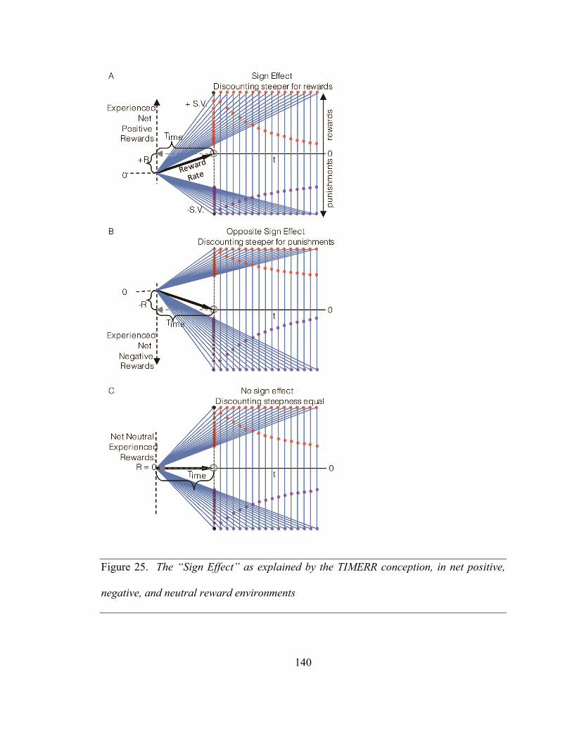
140
Figure 25. The “Sign Effect” as explained by the TIMERR conception, in net positive,
negative, and neutral reward environments
141
A. The sign-effect in a net positive reward environment. Experienced reward history
generates a bias in evaluating equivalently sized outcomes of opposite sign, leading to an
apparent discounting function for rewards that is less steep than that for punishments. B.
The “sign-effect” as predicted by TIMERR for an agent having experienced a net
negative reward environment also exhibits asymmetric discounting functions for rewards
and punishments, yet here, punishments rather than rewards discount less steeply, ie. the
sign of the sign-effect is reversed. C. The absence of a net positive or negative reward
experience leads to the absence of bias in evaluating the worth of rewards and
punishments. Under this condition, outcomes of equivalent magnitudes, be they rewards
or punishment, discount at the same rate. Therefore, given a net neutral reward
experience within an environment, the sign effect will not be observed.

142
3.2.2.9 The Sign Effect
Another so-called anomalous behavior observed in intertemporal decision-making is that
of the “sign-effect” wherein outcomes of equal magnitude but opposite sign are observed
to discount at different rates; specifically, that rewards discount more steeply than
punishments. The origins and necessary conditions of this effect are evident in the
graphical depiction of TIMERR in Figure 25A-C. Here, an agent considers rewards and
punishments of equal magnitude arrayed into the future under three different
environments: net positive (Figure 25A), net negative (Figure 25B), and net neutral
(Figure 25C) outcome environments. Within the first environment (Figure 25A), the
agent has experienced a net positive accumulation of reward, R, over its look back time,
Time, and therefore has a positive experienced rate of reward (black vector). Following
prior convention, realizable reward rates given any outcome selection are depicted as the
slope of the choice vectors (blue) connecting the agent’s past self to its future self having
chosen an option. The intersection of these choice vectors with the y-axis at the present
moment of time yields the outcomes’ respective subjective values. Re-plotting these
subjective values to their corresponding temporal delays produces the temporal
discounting functions for the positive and negative rewards (as all outcomes considered
are of unit magnitude, the y-axis of subjective value is equivalent to a y-axis of subjective
value normalized by unit outcome magnitude). The origin of the sign-effect in a net
rewarding environment is then understood as the effect of reward magnitudes
countermanding opportunity cost, while punishment magnitudes exacerbating
opportunity cost.

143
In Figure 25A, I note that the sign-effect arises due to the opposite impact of magnitude
of rewards and punishments on opportunity cost. Suppose, however, that an agent has
experienced a net negative (punishing) environment (Figure 25B). Should the sign-effect
be observed? In that outcomes of equal magnitude but opposite sign are observed to
discount at different rates, yes, a sign-effect would, under the TIMERR conception, be
observed. However, should the “sign-effect” be defined as rewards discounting more
steeply than equally sized punishment, then no. Rather, TIMERR predicts that in net
negative environments it is punishments that discount more steeply than equally sized
rewards. The sign of the “sign-effect” flips in net negative environments. Why?
Whereas in net rewarding environments there is an opportunity cost associated with any
reward in time, in net punishing environments there is an opportunity gain associated
with any punishment in time. Therefore, the origination of this sign-effect in a net
punishing environment is understood as the effect of punishment magnitudes
countermanding opportunity gain, whereas reward magnitudes combine with opportunity
gain.
What then of the sign-effect if the agent has experienced a net neutral reward
environment? In this case (Figure 25C) there is no opportunity cost/gain associated with
any reward or punishment. Therefore, rewards and punishments of equal magnitude
neither countermand not exacerbate opportunity cost, leading to discounting functions
that are equivalently steep. An important aspect, then, in determining the presence,
severity, and sign of the sign-effect is the nature of the outcome environment
experienced. In conclusion, the “sign effect” (Frederick et al., 2002; Kalenscher &

144
Pennartz, 2008; G. Loewenstein & Prelec, 1992), as the “magnitude effect” (Frederick et
al., 2002; Kalenscher & Pennartz, 2008; G. Loewenstein & Prelec, 1992), is a
consequence of experientially constrained reward rate maximization as conceptualized by
TIMERR, not a flaw in rational decision-making.
3.2.2.10 New perspective on the meaning of the terms in
Equation (3.9)
In the above sections, I have treated Time as representing the total time an agent has spent
within a session, and aest as the ratio of the total reward achieved during this time to Time.
However, real animals face at least three major constraints that limit the validity of this
interpretation: (1) their reinforcement environments are not stationary; (2) there is
increasing computational and metabolic costs associated with integrating over a long
time, and, (3) indefinitely long intervals without reward cannot be sustained by an animal
(while maintaining fitness) even if they were to return the highest long-term reward rate
(e.g., choice between 10,000,000 units of food in 100 days vs. 10 units of food in 0.1
day). Hence, I think that the duration of Time is more appropriately thought of as a “past
integration interval” over which recent reward history (aest) is estimated, instead of the
total time spent in an environment. The value of Time might in fact need to be adjusted to
the current environment so as to make optimal decisions (see Section 3.4 for a longer
discussion). Further, it must be pointed out that the past reward rate (aest) might not be as
simply estimated as the ratio of the rewards accumulated over Time, to Time. This would

145
imply that rewards obtained just beyond Time have zero contribution to the past reward
rate whereas all rewards obtained within Time contribute fully. In fact, I have shown
previously that if the updating of the past reward rate has to be done locally (without
storing every past reward’s magnitude and time of receipt in memory), the past reward
rate has to be calculated using an exponential weighting function (Namboodiri, Mihalas,
Marton, et al., 2014). Hence, since Time is the effective duration over which past reward
rates are estimated, I will refer to it from here on as the “past integration interval” and not
the “look-back time” as in prior sections.
3.2.2.11 Connection to experimental data
In this section, I review experimental data from a wide array of fields that can be
systematized by my theory. For this purpose, I treat typical human and non-human
animal experiments separately as typical human experiments differ from animal
experiments in one fundamental way: humans are often given hypothetical rewards
involving hypothetical delays. However, animals face real rewards requiring real
investments of time. I will first cover non-human animal experiments. But before
considering them separately, I will first discuss commonalities in animal and human
experiments. In both groups, hyperbolic discounting has provided better fits to data than
exponential discounting functions (e.g. G. Ainslie & Monterosso, 2003; G. W. Ainslie,
1974; G. Ainslie, 1975; Benzion et al., 1989; Calvert et al., 2010; Green et al., 1994; Holt
et al., 2003; Kobayashi & Schultz, 2008; Rachlin et al., 1972; Thaler, 1981), as predicted
by DUT (however for an exception, see (Schweighofer et al., 2006)). My theory fits with

146
this observation as Equation (3.9) predicts a temporal discounting function that is a
hyperbolic discounting function minus a constant (aestTime) that depends on the immediate
reinforcement history.
Another finding that is consistently observed across humans and non-human animals is
variability in the discounting steepness within and across individuals (G. Ainslie &
Monterosso, 2003; G. W. Ainslie, 1974; G. Ainslie, 1975; Benzion et al., 1989;
Blanchard et al., 2013; Calvert et al., 2010; Frederick et al., 2002; Green et al., 1994; Holt
et al., 2003; Jimura, Myerson, Hilgard, Braver, & Green, 2009; Kobayashi & Schultz,
2008; Myerson & Green, 1995; Odum, 2011; Pearson et al., 2010; Rachlin et al., 1972;
Richards, Zhang, Mitchell, & de Wit, 1999; Rosati, Stevens, Hare, & Hauser, 2007;
Shamosh et al., 2008; Thaler, 1981). While common accounts of such variability invoke
differences in “personality” (or other psychological/neurological) traits (Warren K Bickel
et al., 2007; Kalenscher & Pennartz, 2008; Madden & Bickel, 2010; Odum, 2011;
Richards et al., 1999; van den Bos & McClure, 2013), I ascribe it a more functional
meaning: variability across subjects reflects variability in the past integration interval,
appropriate for the individuals’ respective reward environments. Relatedly, apparent
differences between subjects may actually reflect differences in experienced past reward
rate (aest in Equation (3.9)). Nonetheless, some variability across subjects may yet lie in
subjects’ innate neural differences, independent of their environment or experience.
3.2.2.11.1 Data from non-human animals
A fundamental prediction of Equation (3.9) is that the discounting steepness will depend
on the past reward rate. This means that, for instance, when the duration between rewards

147
is increased, animals should become more tolerant to delays, since the longer the duration
between rewards, the lower the past reward rate and therefore, the lower the discounting
steepness (Figure 20). Data from (Blanchard et al., 2013) discussed in Section 3.2.1
support this prediction. As mentioned above, they observed lower levels of discounting
steepness when the post-reward delays (equal for both options in experiment 3) were
increased. Since they wished to use this observation to advance a rate-maximizing
equation such as Equation (3.5), they had to further assume that representations of post-
reward delays are biased. As discussed earlier, this is not consistent with many other
experimental results on time perception (e.g. Buhusi & Meck, 2005; Matell & Meck,
2004). A simpler explanation for their data, within a reward-rate maximizing framework
is the one I’ve proposed. Another paper that observes a similar effect in a different task is
(James E Mazur & Biondi, 2011). In their study, they found that the delay at which a
delayed reward is treated as equivalent to a standard reward of fixed magnitude and
delay, depended on the intertrial interval, again consistent with the effect of reducing past
reward rates.
Another key prediction of Equation (3.9) is the “magnitude effect”, as shown in Figure
24. Before considering experimental evidence addressing whether animals show
“magnitude effect”, note that in Figure 24, I assumed the past reward rate to be constant,
or at least equal for both reward options. Is this assumption valid in interpreting results
from experiments?
There are two kinds of experimental designs used to study “magnitude effect” in animals.
One is an “adjusting-amount” or “titration” procedure. In this design, a standard reward

148
option (with fixed delay and magnitude) is compared against an option with an
immediate reward with varying magnitudes. The magnitude of the second option is
adjusted depending on the animal’s previous choice. If the animals choose the second
option, then its magnitude is decreased and vice-versa. Discounting functions obtained
from such experiments did not show any difference in the indifference point—the
magnitude at which both options are treated equivalently—for different magnitudes of
the standard option (Calvert et al., 2010; Freeman, Green, Myerson, & Woolverton, 2009;
Green, Myerson, Holt, Slevin, & Estle, 2004; Green & Myerson, 2004; Richards,
Mitchell, de Wit, & Seiden, 1997). Therefore, these authors conclude that there is no
observable “magnitude effect”. Another kind of experimental design used to study
“magnitude effect” in animals is a “concurrent chains task” (R. C. Grace, Sargisson, &
White, 2012; R. C. Grace, 1994; R. Grace, 1999; Kinloch & White, 2013; Ong & White,
2004). In this design, animals responded to concurrently available options (keys to peck,
for instance) in a “choice phase” so as to access one of two reinforcement schedules
(different rewards at differing delays) in an “outcome phase”. In the earlier versions of
this experiment (R. Grace, 1999; Ong & White, 2004), the magnitude for both options
was equal in one block. Once preferences at that magnitude were measured, observations
were repeated for a different magnitude. In both the above types of experiments, it is
clear that when the magnitude under study was large, so was the past reward rate.
Looking back at Equation (3.9), it is evident that when the past reward rate is
proportional to the reward magnitude, the effect of the reward magnitude cancels out
such that there will be no “magnitude effect”. Interestingly, when the above authors
repeated the “concurrent chains” design with a simultaneous change of magnitude and

149
delay, they observed a “magnitude effect” in pigeons as well as humans (R. C. Grace et
al., 2012; Kinloch & White, 2013). While this result has not been explained yet, it has a
straightforward explanation in my framework: when both magnitude and delay are
changed across reinforcement schedules, the past reward rate will not be simply
proportional (aest would still show a positive correlation with r) to the reward magnitude,
as when only the magnitude was changed. Hence, the aest/r term in the numerator of
Equation (3.9) does not cancel out, revealing the “magnitude effect”.
It is important to point out that a descriptive model of discounting that has been recently
proposed (Killeen, 2009) can indeed fit the “magnitude effect” data in (R. C. Grace et al.,
2012), along with an earlier descriptive model (R. C. Grace, 1994). Interestingly,
Killeen’s additive utility model has mathematical similarities to Equation (3.9). Yet there
is no explanation for why there is an additive term in this model. In my theory, a
subtractive opportunity cost automatically emerges as a direct consequence of
experientially informed rate maximization. Precisely due to this difference, my theory
also predicts that in experimental designs where the subtractive opportunity cost term is
directly proportional to the reward magnitude, there will be no observed “magnitude
effect”. Such data cannot be explained by the additive utility model.
Another prediction of Equation (3.9) is the “sign effect”, as shown in Figure 25. This
prediction is however, methodologically challenging in animals since it is difficult to
create punishments of equal magnitudes as rewards. Nevertheless, it has strong support in
human data, as will be discussed in the next section.

150
The most important prediction, however, of Equation (3.9) is as yet untested. This is the
prediction that as the duration over which past reward rates are estimated increases (or
decreases), the steepness of temporal discounting decreases (or increases). This will
provide the direct falsifiable test of my theory. However, as discussed in the next section,
some indirect evidence from humans supports the above prediction.
3.2.2.11.2 Data from humans
As mentioned earlier, my theory, TIMERR, was developed in the context of optimal
foraging, as we hoped to find an evolutionary argument for discounting. It is in fact
derived from the same starting postulate as Optimal Foraging Theory—that animals
evolved to maximize reward rates (the key difference being that while OFT holds that
only future reward values matter, TIMERR uses the past to inform the maximization of
reward; in some sense, an algorithm for infinite-time-horizon maximization of reward
rates, as postulated in OFT, can be thought of as TIMERR with Time=∞). Hence, the
theory was developed assuming that tasks faced by animals involve real rewards which
require real investments in time. Crucially, all animal tasks that I am aware of require the
animals to invest the delay solely for the purpose of collecting an offered reward. In other
words, in animal tasks, they cannot go about their daily lives seeking other opportunities
for reward while waiting for the promised reward to become available. This is, however,
different for typical human tasks (see Frederick et al., 2002; Kalenscher & Pennartz, 2008
for a review). In typical human tasks, one is asked hypothetical questions involving
hypothetical delays. Let us consider an example: “what would you prefer: $10 in an hour
or $20 in four hours? After the chosen delay expires, we will come find you and pay you

151
the amount”. From anecdotal experience, I have observed that most people prefer $20 in
four hours. How does this vary from typical animal tasks? To see this difference, let us
now consider a different question: “what would you prefer: $10 for waiting in line for an
hour or $20 for waiting in line for four hours? If you wait for the delay, the reward
delivery is certain”. Interestingly, the choice in this question is typically the former: most
people do not want to invest the real four hours for obtaining just $20. Even more
interesting was the observation that anyone that tended to still favor the $20 was a (poor)
graduate student, or currently unemployed. This too, makes sense. If one’s hourly salary
is being cut during the wait time, a rich CEO would never wait four hours for $20,
whereas a graduate student might gladly do so because his/her opportunity cost for
waiting is close to zero. This experiment, though anecdotal, immediately makes it
intuitive that animal experiments are different from typical human experiments involving
hypothetical questions. It also intuitively explains why it is important for animals to
include opportunity costs in their decisions. TIMERR goes beyond this simple realization
only in deriving that the effective time interval over which opportunity costs are
calculated directly determines the steepness of temporal discounting, in addition to the
opportunity cost itself.
In light of this realization that opportunity costs are not directly enforced in typical
human tasks, how can TIMERR explain such data? Does Equation (3.9) apply to such
decisions? I reason that the mathematical form of Equation (3.9) would still apply to such
decisions but the meaning of the terms might be different. Specifically, I believe that Time
would still be a past integration interval, but instead of it being determined by the

152
experience of the subject, it might be determined by the hypothetical choice at hand. For
instance, when one considers choices involving delays of seconds versus choices
involving delays of hours, the past integration interval would adjust flexibly so as to
provide an appropriate time frame for the question at hand. Perhaps this underlies the
observation that when average delays are long, temporal discounting is correspondingly
shallow, compared to when the average delays are short (Carter, Meyer, & Huettel, 2010;
Frederick et al., 2002; Jimura et al., 2009; Kable & Glimcher, 2007; Kalenscher &
Pennartz, 2008; G. Loewenstein & Prelec, 1992; Luhmann, Chun, Yi, Lee, & Wang,
2008; McClure et al., 2004; Rosati et al., 2007; Schweighofer et al., 2006).
The numerator of Equation (3.9), on the other hand, has a subtractive term which reflects
the opportunity cost of waiting. Since there is no real waiting required, one might
suppose that opportunity costs may not exist in such decisions. However, the subtractive
term in the numerator of Equation (3.9) could arise due to two possible reasons: 1) even
though such choices are typically one-shot, it might be implicitly assumed that the
choices will repeat, such that an opportunity cost based on the presented options (e.g.
average reward rate of the presented options) is automatically included in the decision, or
alternatively, 2) humans could incorporate a model of linear risk into such decisions.
In the former possibility, the subjective value of a delayed reward would still be given by
Equation (3.9), but with the aest term representing the average reward rate modeled based
on the current environment (i.e. current options). A prediction of this account would be
that every option presented on a given choice will affect the decision; in a choice between
two options, adding a third decoy option worse than both should have an effect on the

153
choice even though the decoy option would never be picked. A similar observation
(though not in intertemporal decisions) is commonly known as the “decoy effect” or the
“asymmetric dominance effect” in marketing (e.g. Huber, Payne, & Puto, 1982), wherein
adding a decoy option (inferior in all respects to one option but not easily comparable to
the other) automatically shifts preference towards the option that is superior to the decoy.
For a longer discussion on how decisions between options are made in relation to the
environment, see (Ariely, 2008).
To explain the second possibility of a linear risk, let us consider an example: “you are
offered a bag of M&M’s candy containing 100 candies, available to you after 15 minutes.
However, during the 15 minutes, the bag is left open on a table in the hallway. How many
candies would you expect to receive after 15 minutes?” If one assumes that there is a
constant probability of 0.5 that everyone walking by the hallway will pick a candy each,
and one expects 20 people to walk by the hallway in 15 minutes, the expected number of
candies will be: 100 – 0.5*20*1 = 90. If the bag were left out for a time long enough that
at least 200 people are expected to pass by, the number of candies left would be zero.
Thus, the simplest model of risk involved in delaying a reward is that the offered reward
reduces in magnitude at a constant linear rate over time, i.e.
( )dr t kdt
= − (3.10)
If humans do include such a risk model in their decisions, the expected reward that can be
collected after waiting the given delay of t will be r(t)=r-kt. If they simply calculate the
net expected reward rate by dividing this quantity by the past integration interval plus the

154
delay t (just like in the earlier treatment of TIMERR), their subjective value will look like
Equation (3.9), with the linear opportunity cost term (aestt) being replaced by kt, i.e.
( , ) ; 1
0 ;
ime
r kt rSV r t tt kT
rtk
−= <
+
≥
(3.11)
Hence, the mathematical predictions from Equation (3.9) like “magnitude effect” and
“sign effect” would still hold.
There is no first principles reason for why a risk model such as the one envisaged in
Equation (3.10) would be employed by humans in these hypothetical questionnaire tasks.
Nevertheless, a similar risk model has been assumed in a recent successful descriptive
model of discounting (Killeen, 2009). Also, see my previous paper (Namboodiri,
Mihalas, Marton, et al., 2014) for more complex models of risk. Mathematically, the two
possibilities mentioned above are equivalent and result in the same predictions presented
earlier.
Numerous papers evidence “magnitude effect” (Benzion et al., 1989; Frederick et al.,
2002; Green et al., 1994; Green, Myerson, & McFadden, 1997; Thaler, 1981) and “sign
effect” (Benzion et al., 1989; Frederick et al., 2002; Thaler, 1981) in humans. This has
also been repeated using real rewards, instead of hypothetical rewards. In fact, a recent
paper using a task typically done by animals (“concurrent chains task” mentioned in
Section 3.2.2.11.1) in humans choosing between hypothetical rewards also showed a
clear “magnitude effect” (Kinloch & White, 2013). Another prediction of TIMERR is
155
that the size of the “sign effect” will be larger for smaller magnitudes (see Consequences
of the Discounting Function in the Appendix of Namboodiri et al., 2014). This too has
been observed in experiments (Benzion et al., 1989; G. Loewenstein & Prelec, 1992;
Thaler, 1981). Further, Equation (3.9) predicts that a magnitude-like effect for losses (in
net rewarding environments) will be in the opposite direction as that for gains, i.e. losses
of larger magnitudes will be discounted steeper than losses of smaller magnitudes. This
was recently tested in 2012 (Hardisty, Appelt, & Weber, 2012) and found to be true.
Yet another prediction similar to the above effects is that losses will be treated differently
depending on their magnitude (see Consequences of the Discounting Function in the
Appendix of Namboodiri et al., 2014). Specifically, a smaller loss (a loss smaller in
magnitude than the magnitude of the accumulated reward) will become even more of a
loss when delayed, whereas a larger loss becomes less of a loss with additional delay.
Such a differential treatment of losses is also widely observed in experiments (Benzion et
al., 1989; Berns et al., 2006; G. F. Loewenstein, 1987; Mackeigan, Larson, Draugalis,
Bootman, & Burns, 1993; Mischel, Grusec, & Masters, 1969; Redelmeier & Heller,
1993; Yates & Watts, 1975). The above experiments rationalize this result as resulting
from increased “anticipation” of losses (for example, see (G. F. Loewenstein, 1987)).
However, we do not have to make such ad-hoc justifications; it is a natural consequence
of reward rate maximization, as in my theory.
Another “anomalous” observation (from the perspective of DUT) is the “delay-speedup
effect” (Benzion et al., 1989; G. Loewenstein & Prelec, 1992; G. Loewenstein, 1988).
This refers to the observation that subjects expect more compensation for delaying receipt

156
of a reward (from t1 to t2) than they are willing to pay to speed it up by that same amount
(from t2 to t1). There are two potential explanations for this phenomenon. One
explanation, as previously noted by (Killeen, 2009) is that it could simply be a
consequence of recursive discounting, i.e. the subjective value of a reward delayed from
t1 to t2 is the subjective value of the reward at t1 discounted again by the additional delay
of t2-t1. Thus, a reward expected at t1 when delayed to t2 has a subjective value lower than
a reward expected at a delay of t2. I will not mathematically prove this property here for
Equation (3.9) since it is straightforward. One problem, however, with this account (and
the one presented in (Killeen, 2009)) is that if t1 were zero, there is no predicted “delay-
speedup effect”, even though experiments clearly demonstrate an effect even when t1=0
(Benzion et al., 1989; G. Loewenstein & Prelec, 1992; G. Loewenstein, 1988). Another
potential explanation is that whenever subjects are told that they have “received a reward
at time t1”, they automatically incorporate the receipt of that reward into the risk term in
Equation (3.11). This is more easily understood with the M&M’s example. The “delay”
experiment goes thusly: “imagine you have received 100 M&M’s. How many more
M&M’s should I give you such that you are willing to delay receipt by 15 minutes?”
Going back to the calculation above, if you expect that in 15 minutes, the actual number
of M&M’s you receive is 90 (since 20 people take one each at 0.5 probability), you will
require compensation for this assumed reduction as well. On the other hand, the
“speedup” experiment goes thusly: “imagine you will receive 100 M&M’s in 15 minutes.
How many are you willing to pay so as to receive it immediately?” When one evaluates
this question, it makes sense to assume that it is certain that the 100 M&M’s exist after
15 minutes (because it has not been left out in the hallway). Hence, in speeding up its

157
receipt, one only needs to pay for the pure temporal cost (and not the linear risk cost). Of
course, further experiments will be needed to test this hypothesis. Note also that both of
the above arguments make it clear that delaying a reward in multiple steps by short
delays causes it to decay faster than delaying it by the total amount all at once. This effect
has been previously observed and labeled as “subadditivity” (Read, 2001).
In sum, most human discounting tasks differ from animal tasks in a crucial aspect:
humans do not have to wait the corresponding delays. Consequently, the opportunity cost
term in TIMERR should not directly apply to these tasks. However, assuming that
humans employ a simple model of risk (constant decay) in such decisions—similar to an
assumption made previously in a successful descriptive model (Killeen, 2009)—
preserves all of the mathematical qualities of the subjective value of a delayed reward as
derived by TIMERR. Evidence collected across numerous experiments (see Kalenscher
& Pennartz, 2008; G. Loewenstein & Prelec, 1992; Madden & Bickel, 2010 for reviews)
support these predictions. Recently, there have been attempts to test humans on
discounting tasks similar to animal tasks, requiring them to wait out the delays for real
rewards (e.g. Reynolds & Schiffbauer, 2004). More work is needed to know whether
behavior in this task will reproduce the above results (Jimura et al., 2009; Krishnan-Sarin
et al., 2007; Melanko, Leraas, Collins, Fields, & Reynolds, 2009; Reynolds, Penfold, &
Patak, 2008; Reynolds, 2006; Shiels et al., 2009; Smits, Stein, Johnson, Odum, &
Madden, 2013).

158
3.3 Connection between theories of intertemporal
decision-making and time perception
As mentioned early in the Introduction, it is only natural that time perception and
intertemporal decision-making go hand-in-hand since the latter requires the former. It is
also then intuitive to assert that the former is more fundamental than the latter. In this
view, mechanisms of time perception evolved under their own evolutionary pressures,
whereas intertemporal decision-making was only as good as animals’ ability to perceive
the delays to reward. Hence, all prior attempts to connect intertemporal decision-making
and time perception have assumed time perception to be the more fundamental of the two
processes (Bateson, 2003; Cui, 2011; Gibbon, Church, Fairhurst, & Kacelnik, 1988; Alex
Kacelnik & Bateson, 1996; Kim & Zauberman, 2009; Lapied & Renault, 2012a; Ray &
Bossaerts, 2011; Takahashi, Oono, & Radford, 2008; Takahashi, 2005, 2006; Zauberman,
Kim, Malkoc, & Bettman, 2009).
The sine-qua-non of theories of time perception is their treatment of Weber’s law
(Bateson, 2003; Gibbon et al., 1997; Gibbon, 1977; Killeen & Fetterman, 1988; Matell &
Meck, 2000). Weber’s law is easily understood by considering an example. Imagine that
one is tasked with finding the longer rod among two iron rods placed in parallel from just
a glance; no measurements or realignments are allowed. If one of them were a meter and
the other two, the difference should be as clear as night and day. However, if they are a
hundred meters and a hundred and one meters long, this will be considerably more

159
difficult, even though the difference is still one meter. Essentially, Weber’s law states that
the difference between two quantities is judged relative to the quantities themselves.
Weber’s law also appears in timing: it is easier to discriminate one second from two
seconds than to discriminate one hundred seconds from one hundred and one seconds. A
mathematical statement of Weber’s law for timing goes even further. It states that the
precision of perceiving an interval decreases in direct proportion to the interval; in other
words, the error in perception of an interval grows linearly in proportion to the interval.
This relationship is more commonly known as scalar timing, and has been observed
repeatedly in experiments for humans and non-human animals (Allan & Gibbon, 1991;
Russell M Church & Gibbon, 1982; Gibbon et al., 1984, 1997; Gibbon & Church, 1981;
Gibbon, 1977, 1992; Lejeune & Wearden, 2006; Meck & Church, 1987; J. H. Wearden &
Lejeune, 2008).
Before I consider the different theories of time perception and how they explain scalar
timing, I would like to explain how scalar timing can explain non-stationary time
preferences. Recall that the most well-established result on intertemporal decision-
making is that time preferences are non-stationary. Let us reconsider the two example
questions I provided earlier to illustrate this point: “which would you prefer: $100 now or
$105 in a month?” and “which would you prefer: $100 in a year or $105 in a year and
one month?” Considering the above questions from the perspective of scalar timing, it
must be immediately clear that the month of difference in the first question is
“subjectively longer” than the month in the second question (of course, when the
numbers are specified, they should be treated as mathematically equivalent, but animals

160
must estimate such durations from experience). So essentially, even though the interval
between both rewards is constant, the further away the rewards are from the decision, the
harder it is to discriminate between the two delays. Hence, as the delays are perceived to
be more and more similar, the tendency to pick the larger reward should increase. Thus,
scalar timing can lead to non-stationary time preferences.
The above argument is the essence of numerous prior attempts to connect theories of time
perception to theories of intertemporal decision-making (Bateson, 2003; Cui, 2011;
Gibbon et al., 1988; Alex Kacelnik & Bateson, 1996; Stephens, 2002; Zauberman et al.,
2009). In fact, it has also been shown that if the perception of time were logarithmic,
which is consistent with scalar timing, an exponential discounting in subjective time is
mathematically equivalent to a hyperbolic discounting in real time (Takahashi, 2005;
Zauberman et al., 2009). Similar explanations also exist using other non-linear
representations of subjective time (Ray & Bossaerts, 2011). Thus, it has been argued that
the reason for non-stationary intertemporal preferences is because of imperfections in
time perception (Bateson, 2003; Cui, 2011; Gibbon et al., 1988; Alex Kacelnik &
Bateson, 1996; Kim & Zauberman, 2009; Lapied & Renault, 2012a; Ray & Bossaerts,
2011; Takahashi et al., 2008; Takahashi, 2005, 2006; Zauberman et al., 2009). For other
connections between time perception and intertemporal decision-making, see (Balci et
al., 2011; Balci, Freestone, & Gallistel, 2009; Staddon & Cerutti D T, 2003; Wynne &
Staddon, 1988).
Now, let us consider the different theories of time perception. All the theories considered
here pertain to interval timing, i.e. timing in the range of seconds to minutes. Further, I

161
will only consider two of the most popular theories of timing, as my major goal here is in
studying the relationship between intertemporal decision-making and time perception.
For a more thorough review of the models of timing, see the many reviews and primary
articles that have been written on this topic (Ahrens & Sahani, 2011; Almeida & Ledberg,
2010; Buhusi & Meck, 2005; Buonomano & Karmarkar, 2002; Buonomano, 2007;
Gallistel & Gibbon, 2000; Gavornik et al., 2009; Gibbon et al., 1997; Grossberg &
Schmajuk, 1989; Hass, Blaschke, Rammsayer, & Herrmann, 2008; Hass & Herrmann,
2012; Ludvig, Sutton, & Kehoe, 2008; Luzardo, Ludvig, & Rivest, 2013; Machado,
1997; Matell & Meck, 2000, 2004; Mauk & Buonomano, 2004; Meck, 1996; Merchant et
al., 2013; Miall, 1989; Rivest & Bengio Yoshua, 2011; Shankar & Howard, 2012; Simen,
Balci, de Souza, et al., 2011; Simen, Rivest, Ludvig, Balci, & Killeen, 2013; Staddon,
Chelaru, & Higa, 2002; Staddon & Higa, 1999; Teki, Grube, & Griffiths, 2011;
Treisman, 1963; Wackermann & Ehm, 2006).
The most popular theory of timing is the Scalar Expectancy Theory (SET) (Gibbon et al.,
1984; Gibbon, 1977). This theory proposes that there are three different modules working
together to time an interval. The first stage is a pacemaker that produces a continuous
pulse train that is gated on to a second, accumulator, stage upon receipt of a signal to
time. The accumulator counts the number of pulses until the end of the interval being
timed. The total number of accumulated pulses is then compared against a representation
of that interval stored in a reference memory stage. Crucially, the comparison is based on
a ratio-rule so as to achieve scalar timing. Such ratio comparisons are commonly
observed in many timing tasks (Gibbon & Fairhurst, 1994; Gibbon et al., 1997; Gibbon,

162
1992). The most important source of variability in timing (among variability in clock
speed, clock reliability, accumulation, comparator and memory) according to SET is the
variability introduced when a current duration in working memory is compared to a
remembered duration (Gibbon et al., 1984).
A major competitor to SET is the Behavioral Theory of Timing (BeT) (Killeen &
Fetterman, 1988). BeT, too, effectively uses a similar pacemaker-accumulator system.
BeT states that signals that instruct timing onset result in a series of “adjunctive
behavioral states”—a stereotyped sequence of psychological states—that indicate the
passage of time. According to BeT, animals tell time by knowing the position of their
current adjunctive state in relation to the sequence. In the simplest approximation, the
transition time between states was assumed to be exponentially distributed as resulting
from a Poisson clock, thereby making the arrival time of a given state, gamma
distributed. The core assumption of BeT is that the rate of the Poisson accumulation is
proportional to the reinforcement rate. As most timing tasks confound reinforcement rate
with the target interval (since in many tasks, rewards are received only at the end of the
intervals to be timed) (e.g. Killeen & Fetterman, 1988; Killeen, 1975) , the above
assumption means that the standard deviation of the distribution of a given adjunctive
state is proportional to the period of food delivery, thus resulting in scalar timing (Bizo et
al., 1997; Killeen & Fetterman, 1988).
I am not going to review the merits and demerits of the above theories or any of the
alternate theories of timing (Ahrens & Sahani, 2011; Almeida & Ledberg, 2010;
Creelman, 1962; Gallistel & Gibbon, 2000; Gavornik et al., 2009; Grossberg &

163
Schmajuk, 1989; Hass et al., 2008; Karmarkar & Buonomano, 2007; Ludvig et al., 2008;
Luzardo et al., 2013; Machado, 1997; Matell & Meck, 2000, 2004; Meck, 1996;
Merchant et al., 2013; Miall, 1989; Rivest & Bengio Yoshua, 2011; Shankar & Howard,
2012; Simen, Balci, de Souza, et al., 2011; Staddon et al., 2002; Staddon & Higa, 1999;
Teki et al., 2011; Treisman, 1963; Wackermann & Ehm, 2006) here. These can be found
here (Buhusi & Meck, 2005; Gibbon et al., 1997; Matell & Meck, 2000, 2004; Merchant
et al., 2013; Simen et al., 2013). However, a central consideration missing in the above is
that neither really attempts to answer the question of why Weber’s law is true; they only
address how Weber’s law is generated. Clearly, an ideal timing system, free of any noise,
should be able to precisely time any duration. A first-order deviation from this ideal
system would have a constant error in timing at any duration—not an error that increases
in proportion to the duration. So what could be the reason behind a scalar increase in
noise?
One possible solution is to postulate that animals’ timing can only be as good as the
neurons that help them to time. Since we know that neurons are inherently noisy
information processors, timing behaviors will reflect the noise-duration relationship that
neurons produce. Let us now consider the simplest assumption of noisiness in neuronal
firing, i.e. that they fire according to a Poisson process of rate λ. Assume that timing of an
interval is done by counting the number of spikes: the moment the target number of
spikes (say n) has been emitted, the interval is deemed to have expired. Hence, the
expiration of an interval is treated as the arrival time of the nth spike. For a Poisson
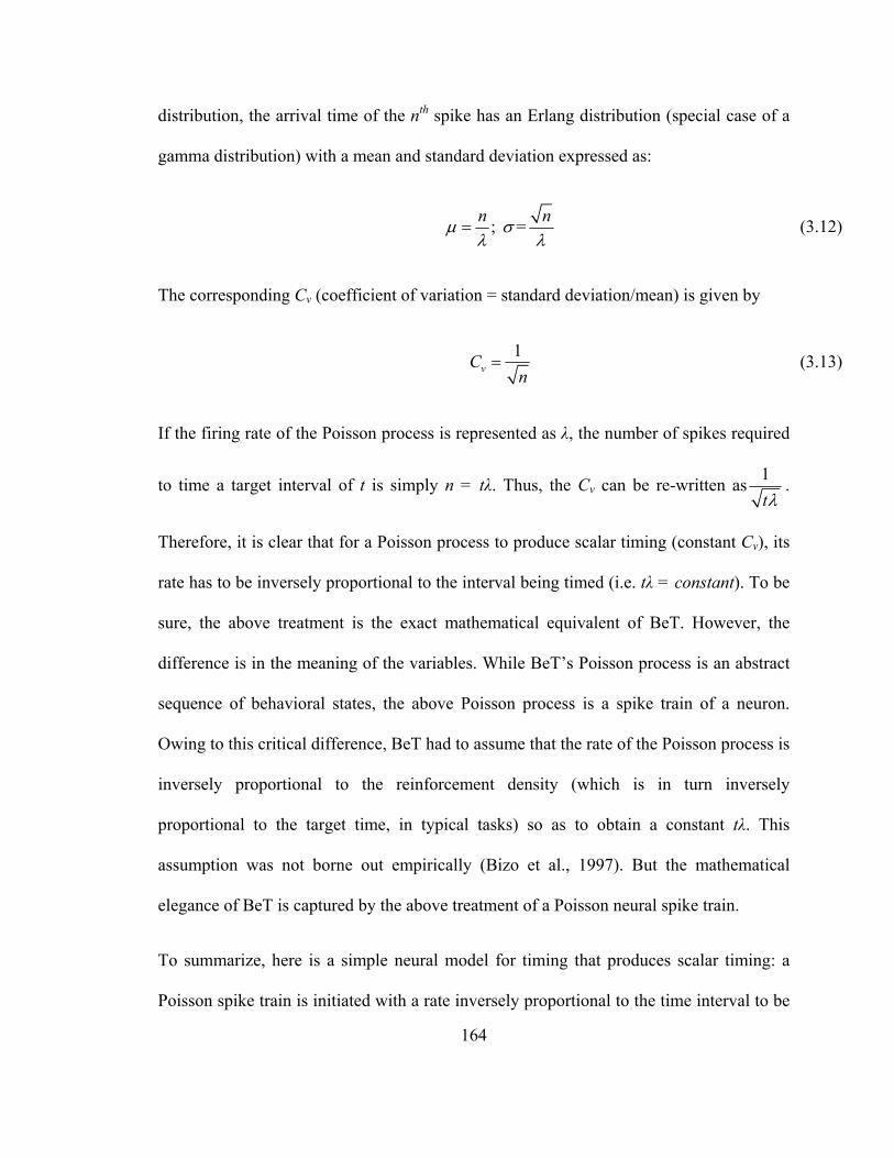
164
distribution, the arrival time of the nth spike has an Erlang distribution (special case of a
gamma distribution) with a mean and standard deviation expressed as:
; =n nμ σλ λ
= (3.12)
The corresponding Cv (coefficient of variation = standard deviation/mean) is given by
1vC
n= (3.13)
If the firing rate of the Poisson process is represented as λ, the number of spikes required
to time a target interval of t is simply n = tλ. Thus, the Cv can be re-written as 1tλ
.
Therefore, it is clear that for a Poisson process to produce scalar timing (constant Cv), its
rate has to be inversely proportional to the interval being timed (i.e. tλ = constant). To be
sure, the above treatment is the exact mathematical equivalent of BeT. However, the
difference is in the meaning of the variables. While BeT’s Poisson process is an abstract
sequence of behavioral states, the above Poisson process is a spike train of a neuron.
Owing to this critical difference, BeT had to assume that the rate of the Poisson process is
inversely proportional to the reinforcement density (which is in turn inversely
proportional to the target time, in typical tasks) so as to obtain a constant tλ. This
assumption was not borne out empirically (Bizo et al., 1997). But the mathematical
elegance of BeT is captured by the above treatment of a Poisson neural spike train.
To summarize, here is a simple neural model for timing that produces scalar timing: a
Poisson spike train is initiated with a rate inversely proportional to the time interval to be

165
timed. The interval is read out as the time to fire a constant threshold of spikes. Let us
now actually calculate some numbers to see if this model is neurally plausible. Typical Cv
values are around 0.1-0.5 in animals (e.g. Matell, Bateson, & Meck, 2006; Matell, Meck,
& Nicolelis, 2003). From Equation (3.13), the number of spikes for the threshold, n, is
approximately 11 (considering a Cv of 0.3). Since n = tλ, this means that in order to time
an interval of 11s, this neuron has to spike at 1Hz, and at 0.1Hz for an interval of 110s.
This firing rate is prohibitively low to be neurally plausible (Simen et al., 2013). Hence,
the above simple neural model which is mathematically equivalent to BeT cannot be
implemented by single neurons.
However, one could imagine the above model to be implemented by a network of
excitatory and inhibitory neurons working so as to produce a balanced integration of
Poisson-like spikes. This is exactly what was done in 2011 by Simen et. al. (Simen, Balci,
de Souza, et al., 2011). They showed that under some simple assumptions, a drift-
diffusion accumulator model of timing comprising Poisson neurons connected into
balanced excitatory and inhibitory networks can work similarly to the mathematical
model presented above. This is shown in Figure 26. In this conception, the mathematics
of BeT is a special case when there is no inhibitory input. I will not go into a more
detailed review of this model, other than to point out that while it retains most of the
mathematical elegance of BeT (and the treatment above), it differs in some quantitative
details; the distribution of the timed interval is inverse-Gaussian and not a gamma
distribution (Simen, Balci, de Souza, et al., 2011).

166
Figure 26. A neural accumulator circuit that implements the simple mathematical
argument (similar to BeT) presented in Section 3.3, modified from Figure 1 in (Simen,
Balci, de Souza, et al., 2011)
There are four different modules in the model. Bistable switches turn on upon timing
onset (“start”) to produce clock speeds adjusted to the target interval (“clock pulse
generator”). An “integrator” produces a linearly rising ramp with the passage of time.
The moment the ramp hits a threshold, a “trigger” turns on indicating the lapse of the
target interval so as to produce the corresponding behavior. Simulations of the model are
shown below to show the different clock speeds producing an inverse-Gaussian
distribution of timed intervals (Simen, Balci, de Souza, et al., 2011).

167
Hence, according to the view of the above theories, scalar timing is a consequence of
noisy information processing by neurons. It must be emphasized that the above models
and theories of timing do not postulate any direct correlations between time perception
and intertemporal decision-making. Recent experimental evidence, however, suggests
otherwise (Baumann & Odum, 2012; Wittmann et al., 2007; Wittmann & Paulus, 2008).
In fact it was found that in general, individuals with better perception of time were more
tolerant to delay (e.g. Baumann & Odum, 2012; Wittmann & Paulus, 2008) (for a more
detailed discussion of these results, see Section 4). This result is not consistent with the
proposition earlier in this section that Weber’s law underlies non-stationary time
preferences. This is because as the perception of time becomes better and the delays
between two options become better discriminated, the tendency to pick the smaller
reward should increase (compared to when the delays are judged to be similar). The
above argument clearly predicts a reduced tolerance to delay with better perception of
time, in contrast to experimental data.
In my theory, I approached the problem of time perception entirely differently. In fact, I
argued that intertemporal decision-making is the more fundamental of the two,
completely opposite to all the prior attempts to connect intertemporal decision-making
and time perception (Bateson, 2003; Cui, 2011; Gibbon et al., 1988; Alex Kacelnik &
Bateson, 1996; Kim & Zauberman, 2009; Lapied & Renault, 2012a; Ray & Bossaerts,
2011; Takahashi et al., 2008; Takahashi, 2005, 2006; Zauberman et al., 2009). I
postulated that time is subjectively represented in such a way that the subjective

168
representation of reward rate (subjective value per unit subjective time) is an accurate
reflection of the true change in expected reward rate.
Using the same symbols as in Section 2.2, this postulate can be expressed as
( , )( ) est
SV r t r aST t t
= − (3.14)
Here, ST(t) is the subjective representation of the true delay to reward t. Solving for the
subjective time, we get the following simple expression
( )1
ime
tST t tT
=+
(3.15)
where Time is the past integration interval, as mentioned in Section 2.2. It must be
emphasized that the subjective representation of the delay is not the subjective report of
the delay; it is how the interval is represented on a subjective neural scale. Figure 27
shows a plot of ST(t) with respect to the actual delay, t. From the plot, it is clear that the
ability to discriminate between intervals decreases as they increase. Further, low values
of Time lead to underproduction of time intervals in a simulated time reproduction task
(Figure 27C,D), appearing as if an internal “clock” is running faster. To see the details of
how this accumulator model works, see (Namboodiri, Mihalas, Marton, et al., 2014), but
an intuitive explanation for why there is an underproduction of intervals for low Time is as
follows: during the production phase of the reproduction task, the time is judged to have
elapsed when the accumulator hits for the first time the remembered threshold (from the
estimation phase). Since the more non-linear the dependence of ST(t) on t (i.e. the lower

169
the value of Time), the more the chance that the accumulation will hit the threshold earlier
(due to the noise in accumulation), and hence, the higher the bias towards an earlier time.

170
Figure 27. Representation of subjective time. Reprinted from (Namboodiri, Mihalas,
Marton, et al., 2014)
A. Two illustrative animals with different values of the past integration interval (Time) are
shown, along with their respective subjective representations of the rewards. B. The
subjective representation of time function as expressed in Equation (3.15) is plotted for
both cases, indicating that the ability to discriminate between the subjective
representations of 40 and 50 seconds is higher for the monkey with Time=300s. C. Results
from a simulated time reproduction task are shown using an accumulator model as
described in (Namboodiri, Mihalas, Marton, et al., 2014), demonstrating the
underproduction of long intervals. D. The underproduction of intervals, interpreted
commonly to result from a faster “clock”, is more pronounced when Time is low. Hence,
individuals with low values of Time will appear as if their internal “clocks” are faster.

171

172
Figure 28. Modified from Figure 3 (Gibbon et al., 1997)
Coefficient of variation across different timing tasks is plotted as a function of the
interval being timed.

173
We showed previously (Namboodiri, Mihalas, Marton, et al., 2014) that a noisy
accumulator model implementing the above equation leads to the following expression of
Cv
2
11 ime
ime
tcT
Cvt
kT
t⎛ ⎞+⎜ ⎟
⎝ ⎠≈ +⎛ ⎞+⎜ ⎟
⎝ ⎠ (3.16)
where c is a constant additive noise in a memory process and k represents the
accumulation noise. If c=0, the above equation implies a constant Cv plus a deviation that
decreases with the past integration interval. As the past integration interval becomes
larger and larger, the coefficient of variation is closer and closer to a constant. In other
words, timing becomes more and more scalar the larger the value of the past integration
interval (and larger the tolerance to delay in intertemporal decisions). Crucially, Equation
(3.16) predicts quantitative deviations from scalar timing, depending on the interval being
timed and the past integration interval. In fact, a review of thirty four studies in 1997 by
the creator and proponents of scalar timing (Gibbon et al., 1997) observed a Cv that
increased with the duration being timed (see Figure 28), as predicted by Equation (3.16)
(assuming constant Time across these experiments). For other studies showing an increase
in Cv at long durations, consistent with Equation (3.16), see (Bizo, Chu, Sanabria, &
Killeen, 2006; Lejeune & Wearden, 1991; Zeiler & Hoyert, 1989; Zeiler & Powell, 1994;
Zeiler, 1991), but also see (Lewis & Miall, 2009) for the opposite pattern. Nevertheless, it
must be pointed out that Equation (3.16) results from specific assumptions (e.g. Poisson-
like noise in accumulation) about the neural implementation of Equation (3.15). It is

174
possible that more detailed and realistic neural implementations might differ from the
approximation expressed in Equation (3.16).
Another key feature of temporal discrimination tasks is the point of subjective equality
(PSE)—the duration which is judged to be equidistant between two intervals to be
discriminated. SET predicts PSE to be at the geometric mean of the two intervals (Allan
& Gibbon, 1991; Gibbon et al., 1984; Gibbon, 1977). This prediction received
considerable experimental support (e.g. Allan & Gibbon, 1991; Church & Deluty, 1977;
Gibbon, 1986; Platt & Davis, 1983) and has been proposed to either result from ratio
comparisons using linear subjective time or from logarithmic subjective time (Gibbon &
Church, 1981). However, a significant number of experiments also show deviations from
the geometric mean (e.g. Kopec & Brody, 2010; J H Wearden, 1991). In fact, in a re-
analysis of some earlier data (claiming PSE at geometric mean) using a more precise
model, (Killeen, Fetterman, & Bizo, 1997) found that the PSE was found to vary between
the harmonic mean and the arithmetic mean. My theory also predicts that the PSE will be
between the harmonic and arithmetic mean depending on the past integration interval.
The lower the past integration interval, the more non-linear the representation of time
becomes and the closer the PSE gets to the harmonic mean. When the past integration
interval is very large, the PSE instead approaches the arithmetic mean. It must be pointed
out that I have not attempted to quantitatively fit the PSE observed in previous studies
because of the difficulty in knowing the value of Time across these studies. However, for a
different model that attempts to systematically explain variance in the PSE, see (Kopec &

175
Brody, 2010). See also (Balci et al., 2011) for an interesting perspective on how differing
abilities to time would dictate different values of optimal PSE.
In sum, prior theories of time perception treat time perception as independent of
intertemporal decision-making. Attempts to connect both have always treated time
perception as more fundamental, implicitly assuming that mechanisms of time perception
evolved under their own selective pressures. The most popular of these models are
accumulator models, in which scalar timing is assumed to result from different sources of
neural variability connected to the accumulation process (e.g. accumulation variability,
pacemaker variability, memory variability etc). However, in TIMERR theory, I postulate
that intertemporal decision-making is more fundamental, i.e. that animals evolved to
maximize reward rates and that scalar timing is a result of representing time subjectively
so that the subjective reward rate accurately represents the change in expected reward
rate (Equation (3.14)). This model is able to explain some experimentally-observed
deviations from Weber’s law (but fails to explain some others) as well as individual
variability in points of subjective equality in temporal discrimination experiments. More
crucially, however, according to my theory, time perception is fundamentally linked to
intertemporal decision-making: the higher the tolerance to delays, the better the
perception of time. Ours is the only current mathematical theory that can explain such
experimentally observed correlations (Barkley et al., 2001; Barratt, 1983; Bauer, 2001;
Baumann & Odum, 2012; Berlin et al., 2004; Berlin & Rolls, 2004; W K Bickel &
Marsch, 2001; Dougherty et al., 2003; Heilbronner & Meck, 2014; Levin et al., 1996;

176
Pine et al., 2010; Reynolds & Schiffbauer, 2004; van den Broek et al., 1992; Wittmann et
al., 2007; Wittmann & Paulus, 2008) systematically.
To revisit, the reason why I treated decision-making as fundamental is that while
decision-making can be clearly treated within the optimization problem of maximizing
reward rates, there is no such well-defined optimization problem for time perception (in
fact, the most optimal model would have a constant precision, independent of the
duration represented). Interestingly, while previous models that connect intertemporal
decision-making and time perception treat the psychophysical observations of time
perception (scalar timing) as a fundamental postulate, I am able to derive approximate
scalar timing from reward rate maximization. I would like to point out that the fact that
such a connection can be made does not prove that time perception indeed evolutionarily
followed the need to maximize reward rates, nor does it mean that every instance of time
perception requires decision-making (making intertemporal decisions, of course,
necessitates the measurement of time). It only suggests that maximizing reward rates
might underlie the evolutionary origin of the psychophysics of time perception.
In the next section, I focus on how variability in the past integration interval leads to
corresponding variability in intertemporal decision-making and time perception.

177
3.4 Impulsivity in the domain of time
As discussed in Section 3.2.2 and Section 3, my theory postulates that the duration over
which the past reward rate is estimated (Time) directly determines the tolerance to delays
in intertemporal decision-making (i.e. the steepness of temporal discounting) and the
non-linearity of time perception. Hence, a fundamental question is how the past
integration interval is determined. We have previously listed a set of qualitative
arguments on this issue (see "Effects of Plasticity in the Past Integration Interval" in
Appendix of Namboodiri et al., 2014) and here, I will present a brief summary of those
arguments.
An optimal value of Time will have to satisfy four criteria: (1) it should maximize the
metabolic fitness of the animal, through (2) reliable estimation of the past reward rate and
temporal delays in the environment (larger the value of Time, better the accuracy in time
perception) so as to (3) appropriately estimate the opportunity cost involved in decisions,
while (4) minimizing computational/memory costs. The essence of this optimization is
the trade-off between maximizing reward rates and minimizing metabolic costs:
integrating over long intervals in stationary environments would lead to better estimates
of opportunity costs, but lead to increased metabolic costs associated with the energy
spent by the brain in its execution. Further, when environments are non-stationary, the
problem becomes even more complicated as one will have to find the duration of history
that appropriately represents the current decisions. I will not attempt a quantitative

178
treatment of this problem here. Similar, but less general, optimization problems have
been investigated elsewhere (Behrens, Woolrich, Walton, & Rushworth, 2007; Bialek,
2005; Courville, Daw, & Touretzky, 2006; Nassar, Wilson, Heasly, & Gold, 2010;
Pearson, Heilbronner, Barack, Hayden, & Platt, 2011; Wilson, Nassar, & Gold, 2013).
I am especially interested in environments that result in low values of the past integration
interval, and consequently steep temporal discounting. This is because steep temporal
discounting has been associated with a set of behavioral disorders under the umbrella of
“impulsivity” (Evenden, 1999; Madden & Bickel, 2010). Below, I will only focus on the
aspects of impulsivity that relate to decisions in the dimension of time.
In a non-stationary environment with a high temporal frequency of instability, the
optimal Time will have to be correspondingly low so as to provide an appropriate
opportunity cost estimate for current decisions. At the other extreme, in a stationary
(stationary refers to time-independent statistics and not low variability in the reward
statistics) environment in which the variability in reward rate is very low, a low Time is
sufficient to appropriately estimate the long-term statistics. Hence, here too, since there is
diminishing benefits in integrating over longer and longer durations, the metabolic costs
will drive down Time. Another instance where Time would be low is when the reward rates
are very high. In a highly rewarding environment, any additional benefit in integrating
over long intervals would be offset by the increase in metabolic costs. Hence, I predict
that individuals living in the above reward environments will discount rewards steeply,
because steep discounting is optimal in these environments. In this conception,
abnormally-steep discounting observed in experiments is not necessarily a sign of a

179
behavioral disorder (viz. impulsivity), but could represent optimality in an individual’s
perceived reward environment. Of course, this does not mean that every instance of
abnormally-steep discounting is optimal; it could also result from aberrations in the brain
mechanisms underlying appropriate setting of Time. Such aberrations might be present in
neurobiological disorders leading to impulsive decision-making as seen, for instance, in
Parkinson’s disease (Housden, O’Sullivan, Joyce, Lees, & Roiser, 2010; Voon & Dalley,
2011; Voon et al., 2010) and schizophrenia (Avsar et al., 2013; Heerey, Robinson,
McMahon, & Gold, 2007; Strauss, Waltz, & Gold, 2014).
Since my theory also predicts that abnormally-steep temporal discounting will be
correlated with highly non-linear time perception, I would predict, for instance, that in a
highly rewarding environment in which Time is low, temporal perception would appear
sped up. This prediction may underlie anecdotal observations that “time flies when you’re
having fun”. My account would also predict that a decrease in reward rate might lead to
temporal perception appearing slowed down. This might explain some recent
observations (Galtress & Kirkpatrick, 2009; Galtress, Marshall, & Kirkpatrick, 2012;
Kirkpatrick, 2014) that cannot be explained by current timing theories (see Galtress et al.,
2012 for a discussion). I would like to point out at this stage that there are other models
that also predict a dependence of time perception on the recent history, arguing that
recently experienced temporal intervals act as a prior for time perception (e.g. (Jazayeri
& Shadlen, 2010)).
As mentioned in Section 3.3, variability in Time is also expected to underlie 1) deviations
from Weber’s law at long durations, and, 2) variations in the point of subjective equality
180
in temporal discrimination tasks. While other models ascribe such observed variability to
variability in properties of the accumulator or other neural variables (e.g. Bizo et al.,
2006; Killeen et al., 1997), I predict that variability within subjects can arise from a drive
to maximize reward rates in varied experimental settings. A strong and unique prediction
of this account is that temporal perception is correlated with intertemporal decision-
making. Experimental observations have supported this prediction (Barkley et al., 2001;
Barratt, 1983; Bauer, 2001; Baumann & Odum, 2012; Berlin et al., 2004; Berlin & Rolls,
2004; W K Bickel & Marsch, 2001; Dougherty et al., 2003; Heilbronner & Meck, 2014;
Levin et al., 1996; Pine et al., 2010; Reynolds & Schiffbauer, 2004; van den Broek et al.,
1992; Wittmann et al., 2007; Wittmann & Paulus, 2008). A stronger, yet untested,
falsifiable prediction is that causing changes in the duration over which past reward rate
is estimated leads to corresponding changes in discounting steepness and time perception.
This is the essence of my theory.
3.5 Conclusion
A rationalization of decision-making in the temporal domain has long been sought, yet an
understanding of this problem remains unfulfilled. I have identified three general reasons
why there has not yet been significant agreement between theories and experimental
observation. The first is that, ever since the first formal attempts to make a reckoning of
how humans and animals regard the cost of time, the notion of a discounting function has

181
pervaded, having been ingrained and reified not as a description of observed behavior but
rather as a thing with agency applied by the agent to determine an outcome’s subjective
value. The second is that intertemporal decision-making has not been framed as reward
rate maximization under the constraint of what is feasibly achievable by an agent given
the unknowable future. The third is that temporal discounting and time perception have
largely been treated as separate problems; when not so, intertemporal decision-making
has been regarded as subordinate to time perception rather than being fundamental.
These historical biases have combined so that the search for the perfect discounting
function, that makes a principled, concise, and full accounting of decision-making in the
time domain, has remained an elusive one.
While I posit that, for these reasons, an unresolved tension between theory and
observation exists, theories of intertemporal decision-making over nearly two centuries
have led to a sophisticated and rich understanding of this issue, from the recognition of an
interplay between the magnitude of an outcome and its cost in time, to its formalization
as a psychological conflict, and subsequently to its reframing as a maximization to
increase fitness. Nonetheless, theories from economics and behavioral ecology, whether
attempting to rationalize intertemporal decision-making within the framework of
discounted utility or of reward-rate maximization, fail to provide satisfactory
explanations for empirical data, or, in the case of descriptive modeling that provides good
fit to observation, fail to provide any normative understanding of why discounting
functions take on their apparent form. Recent experiments (Blanchard et al., 2013;
Pearson et al., 2010), however, have shown that what has been previously regarded as

182
clear evidence that animals do not maximize reward rate results from limits in their
associative learning.
Recognizing that reward rate maximization could then yet be the fundamental principle
behind intertemporal decision-making, I have derived (Namboodiri, Mihalas, Marton, et
al., 2014) from first principles a decision-making algorithm that would lead to reward-
rate maximization under experiential constraints. In this theory, we find that the duration
over which the past reward rate is integrated directly determines the tolerance to delays in
intertemporal decision-making (i.e. the steepness of temporal discounting) and the non-
linearity of time perception. Thereby, I also provide a novel theory of time perception
which can explain hallmark behavioral observations (e.g. Weber’s law, point of
subjective equality). Unique to my theory, I predict that the ability of individuals to
perceive time is correlated with their tolerance to delay in intertemporal decision-making.
Therefore, my theory suggests that aberrant timing behavior seen in a range of
cognitive/behavioral disorders can be rationalized as a consequence of aberrant
integration over experienced reward history. A fundamental test of TIMERR, then, is
assessing whether, as the duration over which past reward rates are estimated increases
(or decreases), the steepness of temporal discounting decreases (or increases). This is the
direct falsifiable test of my theory.

183
Chapter 4. A temporal basis for Weber’s law in value perception
4.1 Introduction
Weber’s law, or approximate Weber’s law, has been observed in the perception of
stimulus features such as weight (Killeen, Cate, & Tran, 1993; Weber, 1978), length
(Akre & Johnsen, 2014; Dehaene & Brannon, 2011; Droit-Volet, 2013), brightness
(Rovamo, Mustonen, & Näsänen, 1995), number (Beran, 2007; Cantlon & Brannon,
2006; Cordes, Gelman, Gallistel, & Whalen, 2001; Droit-Volet, 2013; Gallistel, 2011;
Nieder & Miller, 2003; Whalen, Gallistel, & Gelman, 1999), reward magnitude (Bateson,
Kacelnik, Road, & Ox, 1995; Alex Kacelnik & Bateson, 1996; Killeen et al., 1993), time
(Buhusi & Meck, 2005; Gibbon et al., 1984; Gibbon, 1977; Matell & Meck, 2000),
loudness (Bee, Vélez, & Forester, 2012; Forrest, 1994) etc (Akre & Johnsen, 2014). It
states that the ability to perceive a change in a quantity decreases in proportion to its
magnitude. The fact that our ability to perceive a change in a stimulus often decreases as
its magnitude increases is immediately recognized; for instance, it is more difficult to
perceive an increase of 1g if one is measuring 100g as opposed to when measuring 2g.
Weber’s law, however, states that this decrease in ability to assess magnitude is
proportional to the magnitude of the stimulus, i.e. that it is 50 times more difficult to
perceive a given change around 100g than it is to perceive the same change around 2g.
Even though there is considerable experimental support for the law, its neural or

184
evolutionary origin is unclear (Akre & Johnsen, 2014; Bueti & Walsh, 2009; Walsh,
2003). Further, since animals are often thought to make decisions so as to maximize
reward rates (thus requiring perception of reward magnitude and delays) (Balci et al.,
2011; Blanchard et al., 2013; Namboodiri, Mihalas, Marton, et al., 2014; Stephens &
Krebs, 1986), Weber’s law in the perception of reward magnitudes and delays must affect
such decisions. The mathematical properties of such effects on the decisions of animals
are, however, unclear.
In the previous chapter, I presented a theory of decision-making and time perception that
postulates that the decision of animals regarding delayed outcomes is a consequence of
reward rate maximization in a limited temporal window that includes a past integration
interval (over which experienced reward rate is estimated) and the delay to a given
reward (TIMERR) (Namboodiri, Mihalas, Marton, et al., 2014). I showed that the
decision-making algorithm resulting from this postulate automatically includes an
estimate of opportunity cost and an explicit cost of time. I further showed that it can
explain the breadth of behavioral observations on intertemporal decision-making. The
theory also postulates that time is represented subjectively such that the subjective reward
rate equals the objective change in reward rate, i.e. a subject’s estimate of the subjective
value per unit subjective time accurately represents how much the reward rate of the
current offer exceeds the experienced reward rate. Using this theory, I examine the origin
of Weber’s law in reward magnitude in this chapter and show that the perception of
reward magnitude is correlated with the perception of time, and that the subjective value
change of a delayed reward should also approximately abide by Weber’s law. I also

185
present a novel accumulator model of sensory perception that predicts approximate
Weber’s law for quantities (such as reward magnitude) that are measured over finite
sensory intervals.
4.2 Results
My main aim in this chapter is to study how errors in the subjective representation of an
interval correspondingly affect the subjective value of that reward. To this end, I first
express the subjective value of a delayed reward in terms of the subjective representation
of the delay.
The subjective value of a reward with magnitude r delayed by an interval t as calculated
in TIMERR (Figure 29) is:
( ), 1
est
ime
r a tSV r t tT
−=
+ (6.1)
where Time represents the past integration interval, i.e. the interval over which the past
reward rate (aest) is estimated. Importantly, Time is not a perceived temporal interval, but is
merely the effective interval over which the past reward rate is estimated (e.g. using an
exponential memory filter as in (Namboodiri, Mihalas, & Hussain Shuler, 2014)).

186
Figure 29 Recapping the TIMERR algorithm
The subjective value of a delayed reward (r) is calculated as the immediate reward that
produces the same total reward rate over a window including a past-integration interval
(Time) (over which experienced reward rate is calculated, aest) and the expected delay (t) to
a future reward. The figure shows a ready means to visually depict the subjective value of
a delayed reward, shown as the purple bar at time zero (“now”). Modified from
(Namboodiri, Mihalas, & Hussain Shuler, 2014) and Figure 19.

187
In the above equation, r can be thought of as the magnitude of an offered reward. But a
more rigorous definition of r is the subjective value of an immediate offered reward, i.e.
( ,0)r SV r= .
Correspondingly, the subjective representation of the delay t as expressed in TIMERR is:
( ) 1
ime
tST t tT
=+
(6.2)
Thus, the subjective representation of time is a non-linear mapping and its non-linearity is
controlled by the past integration interval. It is important to emphasize that the subjective
representation of the delay expressed above is not the subjective (verbal) report of an
interval; it can be thought of as the non-linear neural representation of an interval.
Equation (4.1) can now be re-expressed in terms of the subjective representation of time
as shown in Equation (4.2) as
( ) (( ) ( )(, ) ) )( ()1 ( )1
est est est
ime
ime
ST Sr ST t ST tSV r t a t r a t r a tt ST ttST tTT
T ST= − = − = −+
−
(6.3)
Therefore,
( ), ( ) ( )est
ime
rSV r t r a ST tT
= − + (6.4)
Thus, the discounting of a delayed reward is linear with respect to the subjective
representation of that delay. I assume here that the subjective value of a delayed reward is

188
calculated by first measuring the subjective representation of the delay and then linearly
discounting using the form expressed in Equation (4.4). This linear discounting with
respect to the subjective representation of time is a direct result of the postulate of my
theory that animals maximize reward-rates over a limited temporal window including the
past integration interval and the delay to future reward.
4.2.1 Contribution of time measurement error to
the error in subjective value
From this relation, we can now calculate the error in subjective value of a delayed reward
resulting from an error in the representation of subjective time (Figure 30). To this end,
let us denote that the just-noticeable-difference (JND) in the subjective representation
ST(t) of the delay t by δST(t), and that the error in the corresponding subjective value is
denoted by δSV(r,t). For the purpose of this section, I assume that the measurement of the
reward magnitude is noiseless. Then, as the subjective representation of the delay t
increases by its JND, the subjective value will increase by the corresponding error. This
can be expressed mathematically as:
( , ) ( , ) ( )( ( ) ( ))estime
rSV r t SV r t r a ST t ST tT
δ δ+ = − + + (6.5)
From Equations (4.5) and (4.4), we can now calculate the JND in subjective value as
( , ) ( ) ( )estime
rSV r t a ST tT
δ δ= − + (6.6)

189
The negative sign here implies that as the delay increases, the subjective value decreases,
i.e. the value is discounted.
I have previously shown that the error in the subjective representation of time is
approximately linearly related to the subjective representation of time in an accumulator
model (Namboodiri, Mihalas, Marton, et al., 2014), i.e. ( ) ( )ST t kST t cδ = + . The
contribution due to the constant term c can be thought of a constant read-out error and is
quite small except in the limit of ST(t) approaching zero. Substituting this relationship
into Equation (4.6), we get
( , ) ( )( ( ) )estime
rSV r t a kST t cT
δ = − + + (6.7)
Equation (4.7) can also be rewritten using Equation (4.4) as
( , ) ( ) ( ( , ))estime
rSV r t c a k r SV r tT
δ = − + − − (6.8)
From the above equation, it can be seen that the error in subjective value of a delayed
reward is linearly related to the drop in subjective value from time zero due to the
passage of time. Hence, Weber’s law applies to the reduction in subjective value of a
delayed reward due to its delay, i.e. to r-SV(r,t). In other words, as the delay increases
and the subjective value reduces, the error in the change of subjective value due to the
delay is proportional to the change in subjective value. Henceforth, I refer to this as
Weber’s law in value perception.

190
Figure 30 Error in subjective value due to error in time perception
Errors in measurement of the delay to a future reward results in a corresponding error in
subjective value. If the delay to the reward is perceived as earlier by the just-noticeable
difference (JND), the subjective value is perceived as being larger. This error in
subjective value is shown in the red bar and is calculated analytically in Section 4.2.1.

191
Let us now examine the effect of reducing the delay to zero. Since the negative sign in
the above equations only indicates the direction of change, I drop this sign from here on
for the calculation of noise. Thus, when t=0, both Equations (4.7) and (4.8) become
( ,0) ( )estime
rSV r c aT
δ = + (6.9)
Thus, the error in the subjective value of an immediate reward is proportional to the
magnitude of the reward. This is Weber’s law in magnitude perception resulting purely
from an error in the perception of an infinitesimally small immediate delay rather than
arising solely from magnitude measurement error as is commonly believed. Interestingly,
as the past integration interval (Time) increases—leading to an increased accuracy of time
perception (Namboodiri, Mihalas, Marton, et al., 2014)—so does the accuracy of reward
magnitude perception. This is a novel, untested prediction of the account presented here.
This temporal basis of Weber’s law for the perception of reward magnitude also predicts
that the accuracy of magnitude representation reduces when the past reward rate is high.
This too, is a novel, testable prediction and is consistent with the notion that when reward
rate is high, the need to represent rewards accurately (thus incurring greater metabolic
costs) is reduced. The above two predictions regarding the dependence of errors in
subjective value on the past integration interval and the past reward rate is depicted in
Figure 31.

192
Figure 31 Dependence of error in subjective value on past integration interval and past
reward rate

193
A. The Weber fraction of error in subjective value decreases with an increase in the past
integration interval. This is mathematically represented in Equation (4.8). Compared to
Figure 30 (represented as low Time in the graph on the right), the past integration interval
is larger in this panel, thus reducing the error in subjective value while increasing the
subjective value. The Weber fraction is thus smaller. B. The Weber fraction of error in
subjective value increases with an increase in the past reward rate. This is mathematically
represented in Equation (4.8). Compared to Figure 30 (represented as low aest in the
graph on the right), the past reward rate is larger in this panel, thus increasing the error in
subjective value while decreasing the subjective value. The Weber fraction is thus larger.

194
The above treatment indicates that noise in time perception results in reward magnitude
perception that abides by Weber’s law. Yet note that, to calculate the error in subjective
magnitude (resulting purely from the noise in the measurement of the infinitesimally-
small delay to immediate reward), I heretofore have ignored the contribution of noise in
the measurement of the reward magnitude itself. Since we do not know the relative
contributions of these sources of noise, it is possible that the source related to time might
contribute but minimally to the overall error in reward magnitude perception. Therefore,
in the next section, I present a model of sensory perception for reward magnitude, and
then calculate the resulting perceptual error.
4.2.2 Sensory measurement error of reward
magnitude due to evidence accumulation
In this section, I calculate the sensory measurement error of reward magnitude (e.g. error
in the measurement of the volume of a water reward). In some modalities, the sensory
receptor is itself thought to produce scalar noise (Donner, Hemilä, & Koskelainen, 1998;
Matthews, Fain, Murphy, & Lamb, 1990; Nieder & Miller, 2003). While this is possible
in the measurement of reward magnitude, I do not consider this simple solution here as
neural elements in the central nervous system are typically considered to approximate
Poisson processes, which have square-root noise and not linear noise (Rieke, Warland,
van Steveninck, & Bialek, 1999). Rather, I consider errors in ascribing value to a given
reward magnitude as resulting from central and not peripheral processes. While there are

195
other models for Weber’s law in sensation (Deco & Rolls, 2006; Dehaene, 2003;
Shouval, Agarwal, & Gavornik, 2013; Treisman, 1966), ours is based on the fact that the
measurement of any sensory quantity has to be carried out over time.
To this end, I assume that the sensory process for measuring the magnitude is carried out
in time over a small temporal window of sensation. This sensory window is defined as
the time over which there is a constant rate of sensory input. Hence, I assume that the net
perceived reward magnitude is proportional to the time it takes to integrate the sensory
input (e.g. when drinking water at a constant rate, the amount of water obtained is
proportional to the duration of consumption). For an alternative model of sensory
integration, see Appendix A1. In order to evaluate the noise in measurement, I assume
that this sensory integration can be described by an accumulator model similar to
previous decision-making models used for evidence accumulation (e.g. Simen et al.,
2011; Brunton et al., 2013). I further assume that the reward magnitude is represented
linearly and does not undergo a logarithmic transformation, as has been suggested for
number representation (Dehaene, 2003). In the rest of this section, I formalize this
accumulator model using a stochastic differential equation, and then analytically
calculate the time dependence of its mean and variance.
If the neural system carrying out this sensory integration were perfectly noiseless, I can
describe the accumulator model by the following differential equation
; 0t sensorydr adt t t= ≤ ≤ (6.10)

196
Here, rt represents the integrated reward magnitude at a given time. Thus, the measured
reward magnitude r will be the integrated magnitude at the end of the sensory window,
tsensory, i.e. sensorytr r= . The rate of sensory input is denoted by a.
I now relax the assumption that the sensory integration is noiseless. Noise in such an
accumulator system can result from two sources: noise in the sensory input and feedback
noise in the accumulator. I assume that the feedback is a zero mean noise resulting from
balanced excitatory/inhibitory connections, similar to many previous works (e.g. Simen
et al., 2011; Brunton et al., 2013), and that the neurons performing these computations
can all be described as Poisson point processes, i.e. the variance of each source of noise
will be proportional to the corresponding signal. Thus, the variance of the sensory input
will be proportional to the input (a) and the feedback noise will be proportional to rt. I
denote the proportionality constants as b and σ respectively.
For simplicity, I first assume that these two sources of noise are independent and
additive. Since the variance of the sum of two independent sources sum up, the net
variance can be expressed as 2 2tr b aσ + . If we consider the variance of the noise term as
constant throughout the integration, it can be represented by introducing an additional
diffusive term that approximates a Brownian motion with infinitesimal variance of
2 2tr b aσ + into Equation (4.10). Thus, the introduction of these noise sources can be
formally described by the following stochastic differential equation
2 2 ; 0t t t sensorydr adt r b a dW t tσ= + + ≤ ≤ (6.11)

197
Wt represents a standard Wiener process (Brownian motion).
I will analytically solve the time dependence for the first and second moments of the
above accumulator (shown in Equation (4.11)) so as to calculate the mean and variance at
the end of the sensory window.
Taking the expectation values on both sides of Equation (4.11), we get
; 0t sensoryd r adt t t< > = ≤ ≤ (6.12)
where <rt> represents the expectation value of rt. Since <r0>=0, we can write the solution
obtained by integrating from 0 to t as
tr at< > = (6.13)
The time evolution equation for <rt2> can similarly be calculated by applying Ito’s
product rule as
2 2 2 2 2 2 2 2 +( ) =2 2 +( ) ; 0t t t t t t t t t t sensorydr r dr dr ar dt r r b a dW adt r b a dW t tσ σ= + + + + ≤ ≤
(6.14)
Using dt2=0, dWt dt=0 and dWt2=dt and taking the expectations of both sides, we get
2 2 2 2 2 (2< . ) ; 0t t t t sensoryd r ar r b a r b a dt t tσ σ< > = > + < + + > ≤ ≤ (6.15)
Simplifying, we get
2 2 2 (( 2 ) ) ; 0t t sensoryd r a r b a dt t tσ< > = + < > + ≤ ≤ (6.16)

198
Substituting from Equation (4.13) and integrating from 0 to t with the boundary condition
of <rt=02>=0, we get
2
2 2 2 ( 2 ) ; 02t sensorytr a a b at t tσ< > = + + ≤ ≤ (6.17)
Thus, the variance of rt can be calculated as
2 2
2 2 2var( ) = - ; 02t t t sensory
a tr r r b at t tσ< > < > = + ≤ ≤ (6.18)
The coefficient of variation of rt is thus
2 2
CV( ) ; 02t sensory
br t ta at
σ= + < ≤ (6.19)
Since the measured reward magnitude is the integrated magnitude after the sensory
window, the CV of the measurement can be written as
2 2
CV( ) 2
sensory
bra at
σ= + (6.20)
Or
2 2
CV( ) 2
bra r
σ= + (6.21)
If one assumes that the rate of sensory input is a constant, the above equation shows that
except for low reward magnitudes, the CV is a constant, i.e. Weber’s law holds
approximately for reward magnitude perception. If σ2/a is large compared to b2, the

199
constant term will dominate and the CV would be almost exactly constant. These
analytical results are confirmed in numerical simulations as shown in Figure 32.
The mathematics of the accumulator shown in Equation (4.11) is quite similar to
Equation 9 in (Simen, Balci, de Souza, et al., 2011). But there are some significant
differences in the meaning of the terms. First, my model is for reward magnitude
perception, whereas theirs is for time interval production. Second, as a consequence,
while in my model the rate of sensory input is assumed to be a constant, they assume that
the rate of accumulation is tuned for the interval to be timed. For this reason, their model
can produce scalar timing only for time interval production and not for time interval
measurement/perception where the coefficient of variation decreases in inverse
proportion to the square root of the interval (similar to the second term in Equation (4.21)
).
Equations (4.11)-(4.21) assumed that the sensory input noise is additive with respect to
the feedback noise. Instead, if this noise were in fact multiplicative, Equation (4.11)
would change to
2 ; 0t t t sensorydr adt b ar dW t tσ= + ≤ ≤ (6.22)
In this case, the CV can similarly be calculated as (shown in Appendix A
( )2bCV r σ
= (6.23)
Thus, when the sensory and feedback noises multiply, the coefficient of variation is
independent of the magnitude of the sensory signal (a).

200
Again, I performed confirmatory numerical simulations of Equation (4.22), the results of
which are shown in Figure 33. Therefore, if the sensory input noise is multiplicative, the
coefficient of variation is exactly constant, thus making Weber’s law exact. Instead, if the
sensory input noise is additive, the coefficient of variation shows deviations from exact
Weber’s law at low reward magnitudes.

201
Figure 32 Confirmatory simulations (see Section 4.4) of the analytical solution of an
accumulator model in which the sensory and feedback noise combine additively
The red line shows the result of the analytical calculation as expressed in Equation (4.21),
wherein the sensory signal (a), magnitude of sensory noise (b), and the magnitude of
feedback noise (σ) are varied. The black dots show the results of numerical simulation.
The results approximate Weber’s law well but for low reward magnitudes and high
sensory noise (b).

202
Figure 33 Confirmatory simulations (see Section 4.4) of the analytical solution of an
accumulator model in which the sensory and feedback noise combine multiplicatively
The red line shows the result of the analytical calculation as expressed in Equation (4.23)
wherein the sensory signal (a), magnitude of sensory noise (b), and the magnitude of
feedback noise (σ) are varied. The black dots show the results of numerical simulation.
Here, Weber’s law is exact.
203
The accumulator model considered above is similar to the one that I previously proposed
for the representation of subjective time (Namboodiri, Mihalas, Marton, et al., 2014),
with two differences. The most important difference is that whereas subjective time is
assumed to be a non-linear transform of real time, subjective reward is assumed to be
linearly proportional to the real reward. Due to this difference, the reward magnitude
accumulator is analytically tractable, unlike the subjective time accumulator, for which
the analytical solution was approximate (Namboodiri, Mihalas, Marton, et al., 2014). The
other difference is that since the reward magnitude accumulator operates on a sensory
input (unlike the subjective time accumulator), the contribution of this sensory noise has
also been included.
4.2.3 Combined error due to time and magnitude
measurements on subjective value
We now have all the elements to calculate the error in subjective value of a delayed
reward resulting from errors in both magnitude and time measurements (Figure 34).

204
Figure 34 The error in subjective value is affected by errors in the measurement of both
delay (as shown in Figure 30) and reward magnitude
This combined error is calculated analytically in Section 4.2.3.

205
Returning to Equation (4.4), if we consider the effect of adding the JND of both r and
ST(t), we see that while adding the JND of r leads to an increase in the SV(r,t), adding the
JND of ST(t) leads to a decrease (due to temporal discounting). Since we are only
interested in the net error, so as to match the direction of change, we will consider the
effect of error in both r and ST(t) by adding the JND of r and subtracting the JND of
ST(t). Thus, we get the following equation
( , ) ( , ) ( )( ( ) ( ))estime
r rSV r t SV r t r r a ST t ST tTδδ δ δ+
+ = + − + − (6.24)
Therefore, using Equation (4.4), the error in subjective value δSV(r,t) can be written as
( ) ( )( , ) (1 ) ( ) ( )estime ime ime
ST t r r ST tSV r t r a ST tT T T
δ δδ δ δ= − + + + (6.25)
From Equation (4.4), ( , ) ( )( )(1 ) est
ime
SV r t a ST tST tT r
+− = . Therefore Equation (4.25)
becomes
( )( , ) ( ( , ) ( )) ( ) ( )est estime ime
r r r ST tSV r t SV r t a ST t a ST tr T Tδ δ δδ δ= + + + + (6.26)
For simplicity, we consider the exact form of Weber’s law to hold for the sensory
measurement of r. Therefore, we write r lrδ
= , where l is the Weber fraction.
From Equations (4.6) and (4.8), the second term in the R.H.S is equal to
( ) ( ( , ))estime
rc a k r SV r tT
+ + − , where ( ) ( )ST t kST t cδ = + .

206
Before calculating the error in subjective value at any delay, I first calculate its value for
an immediate reward, where t=0 and ST(t)=0. From Equation (4.26), this can be written
as
( ,0) ( )estime ime
r lcrSV r lr c aT T
δ = + + + (6.27)
Simplifying, we get
( ,0) ( (1 ) ) estime ime
c cSV r r l caT T
δ = + + + (6.28)
The above equation obeys Weber’s law for reward magnitude perception, resulting from
errors in both the measurement of magnitude and the measurement of the infinitesimal
delay to an immediate reward. As can be seen, the Weber fraction (slope of δSV(r,0) with
respect to r) depends on Time, the past integration interval. Thus, I predict that even within
an individual, the Weber fraction in the perception of reward magnitude (subjective value
of an immediate reward) can change depending on the context, as the past integration
interval changes. The direction of this change will be such that the better the perception
of time, the better the perception of reward magnitude. Further, as mentioned previously
after Equation (4.9), the above equation also predicts that the larger the experienced
reward rate, the larger the error in perception of reward magnitude. These are the strong
falsifiable predictions of my account.
I now calculate the error in subjective value at a given delay t due to errors in both time
and reward magnitude measurement. From Equation (4.26), I get

207
( ( ) )( , ) ( ( , ) ( )) ( ) ( ( , ))est estime ime
r lr kST t cSV r t l SV r t a ST t c a k r SV r tT T
δ += + + + + − + (6.29)
Simplifying, we get
(1 )( , ) ( ) ( , ) ( ) ( ) ( )est estime ime
lrk l cSV r t l k SV r t la ST t r k caT T
δ += − + + + + + (6.30)
Since I am interested in the noise in subjective value of a constant reward magnitude
delayed by varying amounts, if I treat r as a constant (for now), I can write (using
Equation (4.4)) ( , )( )est
ime
r SV r tST t r aT
−=
+. Grouping the terms that are proportional to SV(r,t)
separately from the other terms, the above equation becomes
(1 )( , ) ( , ) ( )est ime est imeest
est ime ime est ime
a T rk a T rkl cSV r t l k l SV r t r k l caa T r T a T r
δ + ++⎛ ⎞ ⎛ ⎞= − − + + + +⎜ ⎟ ⎜ ⎟+ +⎝ ⎠ ⎝ ⎠
(6.31)
The above equation also abides by Weber’s law. Thus, I have shown that the error in
subjective value of a given reward delayed by different amounts is proportional to the
subjective value at each given delay. Again, the Weber fraction depends on the reward
environment of the animal since it depends on r, aest and Time.
We can also similarly calculate the subjective value error at a given delay for differing
reward magnitudes. To do this, we substitute r as (using Equation (4.4))
( , ) ( )( )1est
ime
SV r t a ST tr ST tT
+=
− in a rewritten version of Equation (4.25) as shown below.

208
( ) ( ( ) )( , ) (1 ) ( ) ( ) ( )est estime ime ime ime
ST t r r lr kST t cSV r t lr c a k a ST tT T T T
δ += − + + + + + (6.32)
Thus,
( )( , ) ( ( , ) ( )) (1 ) ( ( ))est estime
c kST tSV r t l SV r t a ST t r l a c kST tT
δ += + + + + + (6.33)
Or,
( ) ( )( , ) ( , ) (1 ) ( )) ( )(1 ) ( )( ) ( )est
ime ime
c kST t c kST tSV r t SV r t l l a lST t ST t l c kST tT ST t T ST t
δ + +⎛ ⎞ ⎛ ⎞= + + + + + + +⎜ ⎟ ⎜ ⎟− −⎝ ⎠ ⎝ ⎠ (6.34)
where ( )1
ime
tST t tT
=+
.
This too abides by Weber’s law. Thus, I have also shown that the error in subjective
value at a given delay for different reward magnitudes is proportional to the subjective
value.
4.3 Discussion
Previously, I presented a general theory of intertemporal decision-making and time
perception (TIMERR) that explains many well-established observations in these fields
209
(Namboodiri, Mihalas, Marton, et al., 2014). My theory states that the decisions of
animals are a consequence of maximizing reward rates in a limited temporal window
including a past integration interval and the delay to a current reward. Interestingly, I
showed that the representation of time is also related to the past integration interval in my
framework, and that impulsive (low tolerance to delays of rewards) individuals have an
impaired perception of time. I then demonstrated that the error in perception of time is
approximately scalar, with the deviation from exact Weber’s law depending on the past
integration interval.
In this chapter, I extended the results of my prior work to consider the role of error in
time perception on the perception of reward magnitudes and the subjective values of
delayed rewards. I showed that the error in perception of the infinitesimally small delay
to an immediate reward affects the perception of reward magnitude in accordance with
Weber’s law. Since the sensory measurement of the reward must be carried out over time,
I derived Weber’s law in the sensation of reward magnitude by assuming an accumulator
model (for this sensory integration) with a Poisson feedback with balanced
excitation/inhibition. This could be the underlying reason behind the observation of
Weber’s law in the perception of reward magnitude by animals. Subsequently, I showed
that in TIMERR, the combination of errors in both time and reward magnitude
measurement on the subjective value change of a delayed reward also accords with
Weber’s law. Crucially, the Weber fractions are predicted to depend on the reward
history of the animal, thus providing a strong, falsifiable prediction of my theory, along

210
with the predicted correlation between errors in time perception and reward magnitude
estimation.
Superficially, it might be assumed that since the perception of reward magnitude abides
by Weber’s law, so should the subjective value of a delayed reward. In fact, such an
assertion has previously been made (Cui, 2011) without the recognition that this requires
a specific relation between subjective value, reward magnitude, delay to reward, and the
perception of the delay. From the analytical derivation presented above, it is evident that
Weber’s law in subjective value change is a consequence of the special forms of
discounting function (subjective value of a delayed reward divided by the subjective
value of that reward when presented immediately) and subjective time representation that
result from my theory. In fact, if one were to make the standard assumptions of 1)
Weber’s law in reward magnitude measurement, 2) a hyperbolic discounting function (G.
W. Ainslie, 1974; Cui, 2011; Frederick et al., 2002; Kalenscher & Pennartz, 2008), and,
3) linear subjective representation of time that abides by Weber’s law (Gibbon et al.,
1984; Gibbon, 1977), the resultant error in subjective value of a delayed reward is far
from proportional to the subjective value, as I show in Appendix A3.
Recent experiments have shown that the representation of reward magnitude or value is
not just dependent on the reward under consideration, but also on other available options
(Bateson, Healy, & Hurly, 2003; Huber et al., 1982; Louie, Khaw, & Glimcher, 2013). A
recent neuroeconomic model (Louie et al., 2013) employing a divisive normalization
scheme wherein each individual reward is compared against the other available options
can produce such context dependence. In light of these findings, one might question my

211
assumption of an absolute code for reward magnitude, i.e. my assumption that reward
magnitude is represented based only on the magnitude of the reward of interest. It is thus
important to point out that my theory predicts context dependent choices even under the
assumption that the reward magnitude representation is independent of the other available
options. This is because the subjective value of a reward (since every reward is
effectively a delayed reward) is affected by the animal’s estimate of its past reward rate
(Equation (4.1)). Thus, the presence of distracters affects the subjective value of a reward
due to an effect on the past reward rate in experiments involving sequential choices.
Additionally, the current options might affect one’s estimate of experienced reward rate
(Namboodiri, Mihalas, & Hussain Shuler, 2014). Further, as shown in Equations (4.9)
and (4.28), the larger the value of the past reward rate, the larger the error (Weber
fraction) in representation of a reward. Thus, my theory predicts that the larger the value
of the distracter (thereby making the past reward rate larger), the higher the errors in
deciding between two rewards, in accordance with the experimental observations shown
in (Louie et al., 2013). The key difference between my account and the divisive
normalization account (Louie et al., 2013) is that in my account, the context dependence
is due to the estimation of past reward rate, whereas in divisive normalization, the context
dependence is based only on the currently available options.
There have been prior models of how Weber’s law in reward magnitude and time
perception affects decisions of animals in the context of external variability along these
two dimensions (see Kacelnik and Bateson, 1996; Kacelnik and Brito E Abreu, 1998).
These models have been successful at explaining why animals tend to prefer variability in

212
time, but not in reward magnitude, in comparison with fixed options of the same mean
(see Kacelnik and Bateson, 1996; Kacelnik and Brito E Abreu, 1998). However, they do
not propose an origin of Weber’s law for reward magnitude or time, nor do they calculate
the net error due to both sources of noise. Unique to my theory, I predict a systematic
relationship between the reward history of animals and their perception of these
quantities.
4.4 Methods
The confirmatory simulations performed for Figure 32 and Figure 33 integrated
Equations (4.11) and (4.22) respectively using the Euler-Maruyama method. Thus, the
discrete time version of the equations used for Figure 32 and Figure 33 are respectively
2 2 (0,1)t t t tr r a t r b a t Nσ+Δ = + Δ + + Δ
(0,1)t t t tr r a t b ar t Nσ+Δ = + Δ + Δ
where N(0,1) is the standard normal distribution. The step size for integration, Δt, was set
to 0.001 units. The parameters were changed as shown in the figure legend. In each case,
the same random seed was used to initialize the simulations.
213
4.5 Appendix
4.5.1 A1
In the chapter, I assumed that the sensory integration for the measurement of reward
magnitude is carried out at a constant rate and that the net perceived magnitude is
proportional to the time of integration. Instead, it is possible to assume that the sensory
integration is carried out over a constant window and that the rate of accumulation is
proportional to the reward magnitude. This may be more appropriate when the reward
magnitude depends on the quality of the reward (juice vs. water) instead of the quantity
(more water vs. less water). In this case, under the assumption of additive independent
Poisson noise as used for the derivation of Equation (4.20), the coefficient of variation in
the integration would be exactly as shown in Equation (4.20), with the only difference
being that the perceived magnitude r would depend on a and that tsensosry would be a
constant. Hence, in this case, the coefficient of variation would be inversely proportional
to the square root of the reward magnitude, thus not obeying Weber’s law.
If instead the noises are multiplicative as assumed in Equation (4.22), the coefficient of
variation will indeed be a constant as shown in Equation (4.23), independent of the rate
of accumulation. Thus, we see that if the sensory and feedback noise were multiplicative,
Weber’s law would be exact.
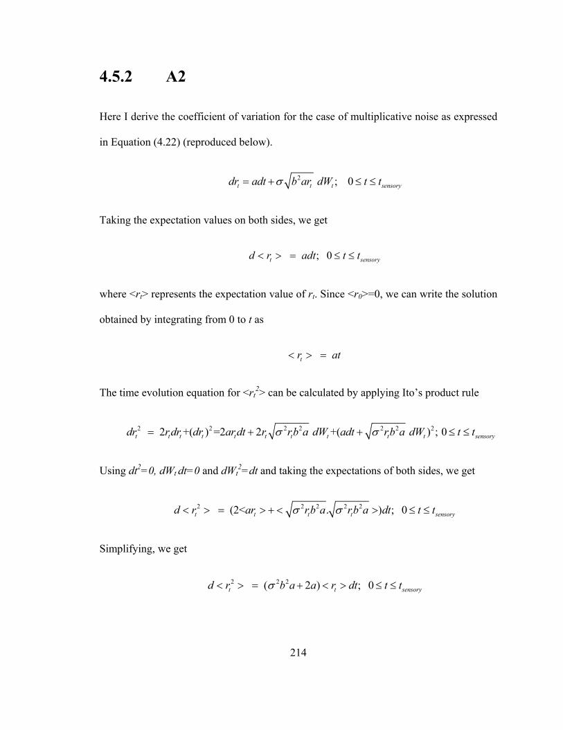
214
4.5.2 A2
Here I derive the coefficient of variation for the case of multiplicative noise as expressed
in Equation (4.22) (reproduced below).
2 ; 0t t t sensorydr adt b ar dW t tσ= + ≤ ≤
Taking the expectation values on both sides, we get
; 0t sensoryd r adt t t< > = ≤ ≤
where <rt> represents the expectation value of rt. Since <r0>=0, we can write the solution
obtained by integrating from 0 to t as
tr at< > =
The time evolution equation for <rt2> can be calculated by applying Ito’s product rule
2 2 2 2 2 2 2 2 +( ) =2 2 +( ) ; 0t t t t t t t t t t sensorydr r dr dr ar dt r rb a dW adt rb a dW t tσ σ= + + ≤ ≤
Using dt2=0, dWt dt=0 and dWt2=dt and taking the expectations of both sides, we get
2 2 2 2 2 (2< . ) ; 0t t t t sensoryd r ar rb a rb a dt t tσ σ< > = > + < > ≤ ≤
Simplifying, we get
2 2 2 ( 2 ) ; 0t t sensoryd r b a a r dt t tσ< > = + < > ≤ ≤

215
Substituting <rt>=at and integrating from 0 to t with the boundary condition of
<rt=02>=0, we get
2
2 2 2 2 ( 2) ; 02t sensorytr a b t tσ< > = + ≤ ≤
Thus, the variance of rt can be calculated as
2 2 2 2
2 2var( ) = - ; 02t t t sensory
a b tr r r t tσ< > < > = ≤ ≤
The coefficient of variation of rt is thus
2
bCV σ=
4.5.3 A3
Here, I calculate the effect of the noise in the measurement of reward magnitude and
delay on the subjective value of a delayed reward that is discounted purely
hyperbolically, with the time perception being linear and showing Weber’s law in error.
This subjective value can be written as
( , )1
rSV r tkt
=+
Since this is not a polynomial function, the JND in SV(r,t) will have to be approximated
using a Taylor series.

216
If we only consider, for now, error in time measurement, the JND for SV(r,t) can be
written as
2 2
2 3
2( , ) ....(1 ) (1 ) 2
kr k r tSV r t tkt kt
δδ δ= − + ++ +
Keeping only the first order term, we get
2( , )( , ) SV r tSV r t k t
rδ δ≈ −
Assuming Weber’s law in time perception, I can write t ctδ = . Substituting into the
above equation, we get
2( , ) ( ( , ))( , )
( , )SV r t r SV r tSV r t kc
r kSV r tδ −
≈ −
Simplifying, we get
2( , ) ( , )( , ) ( ( , )) ( , )SV r t SV r tSV r t c r SV r t cSV r t c
r rδ ≈ − − = −
where the negative sign has been ignored since I am only interested in the magnitude of
the noise. Thus, the error in subjective value of a hyperbolically-discounted reward in the
presence of scalar timing is quadratic with respect to the subjective value, to the first
order.
If I now also include the error in measurement of reward magnitude, the first order term
for δSV(r,t) can be written as

217
2( , )1 (1 )
r krSV r t tkt kt
δδ δ= ++ +
Here, the JND in time perception was decreased so as to maintain the same direction of
change as increasing the reward magnitude by its JND. If δr=lr, this can be written as
2( , )( , ) ( , ) ( , ) SV r tSV r t lSV r t cSV r t c
rδ = + −
This is also quadratic with respect to the subjective value to the first order approximation.
Therefore, even if Weber’s law held in reward magnitude and time perception, under the
common belief of hyperbolic discounting, the subjective value of a delayed reward does
not abide by Weber’s law.

218
Chapter 5. General Discussion
In this thesis, I have attempted to shed light on how animals perceive time and how they
include it in their decisions. To this end, I undertook both an experimental and a
theoretical approach. In my experimental work, I showed that even a primary sensory
area is capable of instructing the production of timed actions. This shows that the brain
does not have exclusive areas involved in sensation, decision-making and motor
production. My work also shows that individual neurons are capable of representing a
temporal interval using sustained modulations during the interval. My collaborators
showed that a model of spiking neuronal network can reproduce the essential features of
our experimental observations.
In my theoretical work, I proposed a simple unifying conceptual framework that explains
how animals make decisions about delayed rewards. It also proposes a simple model of
how time is subjectively represented in the brain. The key finding of the theory is that the
behavior of animals can be understood as the result of maximizing reward rates over
limited temporal intervals. It also assumes that the time interval over which the past
reward rate is calculated is directly related to the temporal interval over which the reward
rate maximization is performed. Interestingly, the theory shows that the interval over
which reward rate maximization is performed directly controls the “patience” (ability to
tolerate delays to rewards) of an individual. Thus, it predicts that in different
environments, the “patience” of an individual will reflect the reward statistics of the
corresponding environment. I then propose that time must be subjectively represented by

219
an individual so that the subjective reward rate equals the objective change in reward
rate. Using this postulate, I show that the subjective representation of time is non-linear
with respect to real time. Importantly, the non-linearity of this map is controlled by the
interval over which reward rate maximization is carried out. Thus, it predicts that there
will be a strong correlation between the “patience” of an individual and the non-linearity
of his/her time perception.
I then calculated the effect of noise in time perception and reward magnitude perception
on the decisions about delayed rewards. I showed that the error in change (with respect to
the subjective value when the delay was zero) of subjective value of a delayed reward is
proportional to the change of subjective value, i.e. that Weber’s law applies to value
perception. Interestingly, the magnitude of this error depends not only on the level of
neuronal noise, but also on the reward statistics of the environment. Further, I
demonstrated that accumulator models for reward magnitude perception will produce
approximate Weber’s law if there is a balanced Poisson feedback in the accumulator.
As is often the case, my work asks more questions than it answers. My experimental
work requires multiple follow-up studies to pinpoint the mechanisms behind V1’s ability
to instruct temporal production. Specifically, it would be interesting to address the
following questions:
1. Is the effect of the optogenetic stimulation dependent on the delay between the visual
stimulus and the stimulation? For the recurrent network model of V1 presented here,
it is likely that the effect of perturbation depends on its timing, even though this has
not been rigorously tested. Thus, it would be interesting to repeat my optogenetic

220
experiment with different delays to stimulation to test out specific predictions
generated by the model. Such experiments would represent additional tests of the
neuronal model.
2. Is V1 the sole instructor of timing in the task? To answer this question, the activity in
V1 will have to be suppressed in a temporally precise way. Currently, this experiment
is technically infeasible to perform in rats. In mice, where the experiment is
technically feasible, it has, however, not been shown that the visually-cued timing
task can be learned. Nevertheless, it is interesting to hypothesize the results of such an
experiment. Since it is technically possible to completely solve the timing task at the
level of V1 (as shown by the neuronal model), it is possible that the sole instructor of
timing in this task is V1. Such a solution would minimize metabolic costs since it
would require fewer number of neurons to be active than if multiple brain regions
were simultaneously controlling timing. However, such a result is inconsistent with
the redundancy in processing that is routinely observed in the brain (Bullmore &
Sporns, 2012). Thus, it is unclear how this trade-off between redundancy in
processing and metabolic cost would be solved by the brain in this task.
3. What is the network mechanism by which timing is generated in V1? A solution to
this problem is presented by the neuronal network model of V1 presented in this
thesis. However, a rigorous experimental test of this model is yet to be undertaken. A
direct test (though currently infeasible) of the model would be to test the strength of
synaptic connections across learning and to show that its development over learning
is as predicted by the model.

221
4. How do the decoder units interact with the intervalkeeper units? The exact network
model for the connections between decoders and intervalkeepers is highly interesting
to study. This is because it is interesting to know whether these connections are
formed spontaneously or through selective learning algorithms. The answer to this
question would indicate whether such network models can also be used more
generally by the brain to solve timing tasks. Experimental access to these connections
would also make it possible to selectively modulate these different network elements.
5. Is V1 also capable of learning new temporal intervals while instructing the production
of temporal intervals? One possible mechanism of behavioral control in this task is
that early in training, behavior is controlled by “higher” brain regions, whereas later
in training when behavioral timing is stereotyped, behavioral control is transferred to
V1 (and possibly other areas). If so, it is interesting to require the animal to learn a
different temporal interval after the learning of a given interval. In this instance of
learning, it would be interesting to test whether it is possible for V1 to learn the new
temporal contingency while being involved in instructing the production of temporal
intervals.
6. How is the output from V1 used to instruct the lick time? What downstream regions
receive this information and how do they process it? The answer to this would clearly
depend on whether or not V1 is the sole instructor of timing in this task. If so, it
would be interesting to test how the connection between V1 and the lick controller
develops over the course of learning. If not, it would be interesting to study how the
different regions involved in behavioral control in this task communicate with one
another and the downstream decoding area.

222
7. Are other regions in the brain capable of instructing temporal interval production in
appropriate contexts? It would be unlikely that this ability to instruct timing of actions
using sustained modulations of firing rate is special to V1. The recurrent network
model presented here could easily be present in other brain regions. Thus, it would be
interesting to test whether the results obtained here for V1 could also be obtained for
other brain regions in appropriate contexts.
The theoretical work also raises several important questions that need to be addressed.
Below is a list of such questions. This list is, by no means, exhaustive.
1. Is the time interval over which reward rate is maximized directly related to the
interval over which past reward rate is calculated? This is the direct falsifiable test of
TIMERR. Even though TIMERR is capable of explaining numerous behavioral
observations in intertemporal decision-making, whether or not it stands the test of
time will be determined by the verification of this core postulate of TIMERR.
2. Is the decision-making of animals fully described by the TIMERR algorithm?
3. What is the optimal interval over which past reward rate is estimated? How does this
depend on the statistics of the environment? Addressing this question would require
solving a much more general optimization problem than has been treated by this
thesis. It would require solving for the optimal Time that maximizes reward rate for a
given environment.
4. Is the experimentally-measured past integration interval consistent with the above
calculations?

223
5. Is the representation of subjective time non-linear? Does this non-linearity change
within a subject?
6. Is the correlation between the steepness of temporal discounting and the non-linearity
of time perception quantitatively explained by TIMERR?
7. What is the mechanism by which animal brains solve the intertemporal decision-
making problem? It would be interesting to test how the different computations
incorporated by TIMERR are solved by different regions of the brain.
8. How is subjective time neurally represented?
As can be seen, the list of unanswered questions is long. I finish this thesis with the
sincere hope that my work has at least contributed (if minimally) to our understanding of
how animals perceive time and use it in their decision-making.

224
BIBLIOGRAPHY
Ahrens, M. B., & Sahani, M. (2011). Observers exploit stochastic models of sensory
change to help judge the passage of time. Current Biology : CB, 21(3), 200–6.
doi:10.1016/j.cub.2010.12.043
Ainslie, G. (1975). Specious reward: A behavioral theory of impulsiveness and impulse
control. Psychological Bulletin, 59(4), 257–72.
Ainslie, G., & Monterosso, J. (2003). Hyperbolic discounting as a factor in addiction: A
critical analysis. In R. E. Vuchinich & N. Heather (Eds.), Choice, Behavioral
Economics and Addiction (First., pp. 35–61). Pergamon.
Ainslie, G. W. (1974). Impulse control in pigeons. Journal of the Experimental Analysis
of Behavior, 21(3), 485–9.
Akre, K. L., & Johnsen, S. (2014). Psychophysics and the evolution of behavior. Trends
in Ecology & Evolution, 29(5), 291–300. doi:10.1016/j.tree.2014.03.007
Allan, L. G. (1979). The perception of time. Perception & Psychophysics, 26(5), 340–
354. doi:10.3758/BF03204158
Allan, L. G., & Gibbon, J. (1991). Human Bisection at the Geometric Mean. Learning
and Motivation, 22, 39–58.

225
Almeida, R., & Ledberg, A. (2010). A biologically plausible model of time-scale
invariant interval timing. Journal of Computational Neuroscience, 28(1), 155–75.
doi:10.1007/s10827-009-0197-8
al-Nowaihi, A., & Dhami, S. (2008). A general theory of time discounting : The
reference-time theory of intertemporal choice (No. 08/22) (Vol. 91).
Ariely, D. (2008). Predictably Irrational: The Hidden Forces That Shape Our Decisions.
New York: HarperCollins.
Avsar, K. B., Weller, R. E., Cox, J. E., Reid, M. A., White, D. M., & Lahti, A. C. (2013).
An fMRI investigation of delay discounting in patients with schizophrenia. Brain
and Behavior, 3(4), 384–401. doi:10.1002/brb3.135
Ayaz, A., Saleem, A. B., Schölvinck, M. L., & Carandini, M. (2013). Locomotion
controls spatial integration in mouse visual cortex. Current Biology : CB, 23(10),
890–4. doi:10.1016/j.cub.2013.04.012
Balci, F., Freestone, D., & Gallistel, C. R. (2009). Risk assessment in man and mouse.
Proceedings of the National Academy of Sciences, 106(7), 2459–2463.
doi:10.1073/pnas.0906213106
Balci, F., Freestone, D., Simen, P., Desouza, L., Cohen, J. D., & Holmes, P. (2011).
Optimal temporal risk assessment. Frontiers in Integrative Neuroscience,
5(September), 56. doi:10.3389/fnint.2011.00056

226
Barkley, R. A., Edwards, G., Laneri, M., Fletcher, K., & Metevia, L. (2001). Executive
functioning, temporal discounting, and sense of time in adolescents with attention
deficit hyperactivity disorder (ADHD) and oppositional defiant disorder (ODD).
Journal of Abnormal Child Psychology, 29(6), 541–56.
Barratt, S. (1983). THE BIOLOGICAL THE SIGNIFICANCE BASIS OF
IMPULSIVENESS : OF TIMING AND RHYTHM. Personality and Individual
Differences, 4(4), 387–391.
Bateson, M. (2003). Interval timing and optimal foraging. In W. H. Meck (Ed.),
Functional and Neural Mechanisms of Interval Timing (pp. 113–141). Boca-Raton,
Florida: CRC Press.
Bateson, M., Healy, S. D., & Hurly, T. A. (2003). Context-dependent foraging decisions
in rufous hummingbirds. Proceedings. Biological Sciences / The Royal Society,
270(1521), 1271–6. doi:10.1098/rspb.2003.2365
Bateson, M., & Kacelnik, A. (1996). Rate currencies and the foraging starling: the fallacy
of the averages revisited. Behavioral Ecology, 7(3), 341–352.
doi:10.1093/beheco/7.3.341
Bateson, M., Kacelnik, A., Road, S. P., & Ox, O. (1995). Accuracy of memory for
amount in the foraging starling , Sturnus vulgaris. Animal Behaviour, 50, 431–443.

227
Bauer, L. O. (2001). Antisocial personality disorder and cocaine dependence: their effects
on behavioral and electroencephalographic measures of time estimation. Drug and
Alcohol Dependence, 63(1), 87–95.
Baumann, A. A., & Odum, A. L. (2012). Impulsivity, risk taking, and timing.
Behavioural Processes, 90(3), 408–14. doi:10.1016/j.beproc.2012.04.005
Bee, M. A., Vélez, A., & Forester, J. D. (2012). Sound level discrimination by gray
treefrogs in the presence and absence of chorus-shaped noise. The Journal of the
Acoustical Society of America, 131(5), 4188–95. doi:10.1121/1.3699271
Behrens, T. E. J., Woolrich, M. W., Walton, M. E., & Rushworth, M. F. S. (2007).
Learning the value of information in an uncertain world. Nature Neuroscience,
10(9), 1214–21. doi:10.1038/nn1954
Bennett, S. M. (2002). Preference reversal and the estimation of indifference points using
a fast-adjusting delay procedure with rats. University of Florida.
Benzion, U., Rapoport, A., Yagil, J., Science, S. M., & Mar, N. (1989). Discount Rates
Inferred from Decisions : An Experimental Study. Management Science, 35(3), 270–
284.
Beran, M. J. (2007). Rhesus monkeys (Macaca mulatta) enumerate large and small
sequentially presented sets of items using analog numerical representations. Journal
of Experimental Psychology. Animal Behavior Processes, 33(1), 42–54.
doi:10.1037/0097-7403.33.1.42

228
Berlin, H. A., & Rolls, E. T. (2004). Time perception, impulsivity, emotionality, and
personality in self-harming borderline personality disorder patients. Journal of
Personality Disorders, 18(4), 358–78. doi:10.1521/pedi.18.4.358.40349
Berlin, H. A., Rolls, E. T., & Kischka, U. (2004). Impulsivity, time perception, emotion
and reinforcement sensitivity in patients with orbitofrontal cortex lesions. Brain : A
Journal of Neurology, 127(Pt 5), 1108–26. doi:10.1093/brain/awh135
Berns, G. S., Chappelow, J., Cekic, M., Zink, C. F., Pagnoni, G., & Martin-Skurski, M.
E. (2006). Neurobiological substrates of dread. Science, 312(5774), 754–8.
doi:10.1126/science.1123721
Bialek, W. (2005). Should you believe that this coin is fair? Neurons and Cognition;
Quantitative Methods.
Bickel, W. K., & Marsch, L. a. (2001). Toward a behavioral economic understanding of
drug dependence: delay discounting processes. Addiction, 96(1), 73–86.
doi:10.1080/09652140020016978
Bickel, W. K., Miller, M. L., Yi, R., Kowal, B. P., Diana, M., & Pitcock, J. A. (2007).
Behavioral and Neuroeconomics of Drug Addiction: Competing Neural Systems and
Temporal Discounting Processes. Drug Alcohol Depend., 90(Suppl 1), S85–S91.
Bizo, L. A., Chu, J. Y. M., Sanabria, F., & Killeen, P. R. (2006). The failure of Weber’s
law in time perception and production. Behavioural Processes, 71(2-3), 201–10.
doi:10.1016/j.beproc.2005.11.006

229
Bizo, L. A., White, K. G., Harper, D., Ruske, A., Swain, N., & Rose, S. (1997). Timing
With Controlled Reinforcer Density : Implications for Models of Timing. Journal of
Experimental Psychology. Animal Behavior Processes, 23(1), 44–55.
Blanchard, T. C., Pearson, J. M., & Hayden, B. Y. (2013). Postreward delays and
systematic biases in measures of animal temporal discounting. Proceedings of the
National Academy of Sciences of the United States of America, 110(38), 15491–6.
doi:10.1073/pnas.1310446110
Bohm-Bawerk, E. von. (1889). Capital and Interest (1970th ed.). South Holland:
Libertarian Press.
Brody, C. D., Hernandez, A., Zainos, A., & Romo, R. (2003). Timing and Neural
Encoding of Somatosensory Parametric Working Memory in Macaque Prefrontal
Cortex. Cerebral Cortex, 13(11), 1196–1207. doi:10.1093/cercor/bhg100
Brosch, M., Selezneva, E., & Scheich, H. (2011). Representation of reward feedback in
primate auditory cortex. Frontiers in Systems Neuroscience, 5(February), 5.
doi:10.3389/fnsys.2011.00005
Brunton, B. W., Botvinick, M. M., & Brody, C. D. (2013). Rats and humans can
optimally accumulate evidence for decision-making. Science (New York, N.Y.),
340(6128), 95–8. doi:10.1126/science.1233912
Bueti, D., & Walsh, V. (2009). The parietal cortex and the representation of time, space,
number and other magnitudes. Philosophical Transactions of the Royal Society of

230
London. Series B, Biological Sciences, 364(1525), 1831–40.
doi:10.1098/rstb.2009.0028
Buhusi, C. V, & Meck, W. H. (2005). What makes us tick? Functional and neural
mechanisms of interval timing. Nature Reviews Neuroscience, 6(10), 755–65.
doi:10.1038/nrn1764
Bullmore, E., & Sporns, O. (2012). The economy of brain network organization. Nature
Reviews Neuroscience, 13(5), 336–49. doi:10.1038/nrn3214
Buonomano, D. V. (2000). Decoding temporal information: A model based on short-term
synaptic plasticity. The Journal of Neuroscience : The Official Journal of the Society
for Neuroscience, 20(3), 1129–41.
Buonomano, D. V. (2007). The biology of time across different scales. Nature Chemical
Biology, 3(10), 594–597.
Buonomano, D. V, & Karmarkar, U. R. (2002). How do we tell time? The Neuroscientist,
8(1), 42–51.
Buonomano, D. V, & Laje, R. (2010). Population clocks: motor timing with neural
dynamics. Trends in Cognitive Sciences, 14(12), 520–7.
doi:10.1016/j.tics.2010.09.002

231
Buonomano, D. V, & Maass, W. (2009). State-dependent computations: spatiotemporal
processing in cortical networks. Nature Reviews Neuroscience, 10(2), 113–25.
doi:10.1038/nrn2558
Burger, R. M., Fukui, I., Ohmori, H., & Rubel, E. W. (2011). Inhibition in the balance:
binaurally coupled inhibitory feedback in sound localization circuitry. Journal of
Neurophysiology, 106(April 2011), 4–14. doi:10.1152/jn.00205.2011
Calvert, A. L., Green, L., & Myerson, J. (2010). Delay discounting of qualitatively
different reinforcers in rats. Journal of the Experimental Analysis of Behavior, 93(2),
171–84. doi:10.1901/jeab.2010.93-171
Cantlon, J. F., & Brannon, E. M. (2006). Shared system for ordering small and large
numbers in monkeys and humans. Psychological Science, 17(5), 401–6.
doi:10.1111/j.1467-9280.2006.01719.x
Cardinal, R. N., Pennicott, D. R., Sugathapala, C. L., Robbins, T. W., & Everitt, B. J.
(2001). Impulsive choice induced in rats by lesions of the nucleus accumbens core.
Science (New York, N.Y.), 292(5526), 2499–501. doi:10.1126/science.1060818
Carter, R. M., Meyer, J. R., & Huettel, S. a. (2010). Functional neuroimaging of
intertemporal choice models: A review. Journal of Neuroscience, Psychology, and
Economics, 3(1), 27–45. doi:10.1037/a0018046
Charnov, E. L. (1976a). Optimal Foraging, the Marginal Value Theorem. Theoretical
Population Biology, 9(2), 129–136.

232
Charnov, E. L. (1976b). Optimal Foraging: Attack Strategy of a Mantid. The American
Naturalist, 110(971), 141–151.
Chubykin, A. A., Roach, E. B., Bear, M. F., & Shuler, M. G. H. (2013). A cholinergic
mechanism for reward timing within primary visual cortex. Neuron, 77(4), 723–35.
doi:10.1016/j.neuron.2012.12.039
Chung, S., & Herrnstein, R. J. (1967). CHOICE AND DELAY OF REINFORCEMENT.
Journal of the Experimental Analysis of Behavior, 10(1), 67–74.
Church, R. M., & Deluty, M. Z. (1977). Bisection of temporal intervals. Journal of
Experimental Psychology. Animal Behavior Processes, 3(3), 216–28.
Church, R. M., & Gibbon, J. (1982). Temporal generalization. Journal of Experimental
Psychology. Animal Behavior Processes, 8(2), 165–86.
Cordes, S., Gelman, R., Gallistel, C. R., & Whalen, J. (2001). Variability signatures
distinguish verbal from nonverbal counting for both large and small numbers.
Psychonomic Bulletin & Review, 8(4), 698–707.
Courville, A. C., Daw, N. D., & Touretzky, D. S. (2006). Bayesian theories of
conditioning in a changing world. Trends in Cognitive Sciences, 10(7), 294–300.
doi:10.1016/j.tics.2006.05.004
Creelman, C. D. (1962). Human Discrimination of Auditory Duration. Journal of the
Acoustical Society of America, 34(5), 582–593.

233
Cui, X. (2011). Hyperbolic discounting emerges from the scalar property of interval
timing. Frontiers in Integrative Neuroscience, 5(June), 24.
doi:10.3389/fnint.2011.00024
Deco, G., & Rolls, E. T. (2006). Decision-making and Weber’s law: a neurophysiological
model. The European Journal of Neuroscience, 24(3), 901–16. doi:10.1111/j.1460-
9568.2006.04940.x
Dehaene, S. (2003). The neural basis of the Weber-Fechner law: a logarithmic mental
number line. Trends in Cognitive Sciences, 7(4), 145–147.
Dehaene, S., & Brannon, E. (Eds.). (2011). Space, Time and Number in the Brain (1st
ed.). San Diego: Academic Press: Elsevier Inc.
Dickinson, A. (1980). Contemporary Animal Learning Theory. Cambridge: Cambridge
University Press.
Donner, K., Hemilä, S., & Koskelainen, a. (1998). Light adaptation of cone
photoresponses studied at the photoreceptor and ganglion cell levels in the frog
retina. Vision Research, 38(1), 19–36.
Dougherty, D. M., Bjork, J. M., Harper, A. R., Mathias, C. W., Moeller, G. F., & Marsh,
D. M. (2003). Validation of the Immediate and Delayed Memory Tasks in
Hospitalized Adolescents With Disruptive Behavior Disorders. The Psychological
Record, 53, 509–532.

234
Droit-Volet, S. (2013). Emotion and magnitude perception: number and length bisection.
Frontiers in Neurorobotics, 7(December), 24. doi:10.3389/fnbot.2013.00024
Drouhin, N. (2009). Hyperbolic discounting may be time consistent. Economics Bulletin,
29(4), 2549–2555.
Evenden, J. L. (1999). Varieties of impulsivity. Psychopharmacology, 146(4), 348–61.
Fehr, E. (2002). The economics of impatience. Nature, 415(6869), 269–72.
doi:10.1038/415269a
Felleman, D. J., & Van Essen, D. C. (1991). Distributed hierarchical processing in the
primate cerebral cortex. Cerebral Cortex, 1(1), 1–47.
Fishburn, P. C., & Rubinstein, A. (1982). Time Preference. International Economic
Review, 23(3), 677–694.
Fisher, I. (1930). The Theory of Interest. New York: Macmillan.
FitzGerald, T. H. B., Friston, K. J., & Dolan, R. J. (2013). Characterising reward outcome
signals in sensory cortex. NeuroImage, 83, 329–34.
doi:10.1016/j.neuroimage.2013.06.061
Fitzpatrick, D., Lund, J. S., Schmechel, D. E., & Towles, a C. (1987). Distribution of
GABAergic neurons and axon terminals in the macaque striate cortex. The Journal
of Comparative Neurology, 264(1), 73–91. doi:10.1002/cne.902640107

235
Fontanini, A., & Katz, D. B. (2008). Behavioral states, network states, and sensory
response variability. Journal of Neurophysiology, 100(3), 1160–8.
doi:10.1152/jn.90592.2008
Forrest, T. G. (1994). From Sender to Receiver : Propagation and Environmental Effects
on Acoustic Signals. American Zoologist, 34(6), 644–654.
Frederick, S., Loewenstein, G., Donoghue, T. O., & Donoghue, T. E. D. O. (2002). Time
Discounting and Time Preference : A Critical Review. Journal of Economic
Literature, 40(2), 351–401.
Freeman, K. B., Green, L., Myerson, J., & Woolverton, W. L. (2009). Delay discounting
of saccharin in rhesus monkeys. Behavioural Processes, 82(2), 214–8.
doi:10.1016/j.beproc.2009.06.002
Gallistel, C. R. (2011). Mental magnitudes. In S. Dehaene & E. Brannon (Eds.), Space,
Time and Number in the Brain (1st ed., Vol. 1, pp. 3–12). San Diego: Academic
Press: Elsevier Inc. doi:10.1016/B978-0-12-385948-8.00001-3
Gallistel, C. R., & Gibbon, J. (2000). Time, Rate, and Conditioning. Psychological
Review, 107(2), 289–344.
Galtress, T., & Kirkpatrick, K. (2009). Reward value effects on timing in the peak
procedure. Learning and Motivation, 40(2), 109–131.
doi:10.1016/j.lmot.2008.05.004

236
Galtress, T., Marshall, A. T., & Kirkpatrick, K. (2012). Motivation and timing: clues for
modeling the reward system. Behavioural Processes, 90(1), 142–53.
doi:10.1016/j.beproc.2012.02.014
Gavornik, J. P., & Bear, M. F. (2014). Learned spatiotemporal sequence recognition and
prediction in primary visual cortex. Nature Neuroscience, 2014(March).
doi:10.1038/nn.3683
Gavornik, J. P., & Shouval, H. Z. (2011). A network of spiking neurons that can
represent interval timing: mean field analysis. Journal of Computational
Neuroscience, 30(2), 501–13. doi:10.1007/s10827-010-0275-y
Gavornik, J. P., Shuler, M. G. H., Loewenstein, Y., Bear, M. F., & Shouval, H. Z. (2009).
Learning reward timing in cortex through reward dependent expression of synaptic
plasticity. Proceedings of the National Academy of Sciences of the United States of
America, 106(16), 6826–31. doi:10.1073/pnas.0901835106
Genovesio, A., Tsujimoto, S., & Wise, S. P. (2006). Neuronal activity related to elapsed
time in prefrontal cortex. Journal of Neurophysiology, 95(January 2006), 3281–
3285. doi:10.1152/jn.01011.2005
Genovesio, A., Tsujimoto, S., & Wise, S. P. (2009). Feature- and order-based timing
representations in the frontal cortex. Neuron, 63(2), 254–66.
doi:10.1016/j.neuron.2009.06.018

237
Ghazanfar, A. A., & Schroeder, C. E. (2006). Is neocortex essentially multisensory?
Trends in Cognitive Sciences, 10(6), 278–85. doi:10.1016/j.tics.2006.04.008
Gibbon, J. (1977). Scalar Expectancy Theory and Weber’s Law in Animal Timing.
Psychological Review, 84(3), 279–325.
Gibbon, J. (1986). The structure of subjective time: How time flies. The Psychology of
Learning and Motivation, 20, 105–135.
Gibbon, J. (1992). Ubiquity of Scalar Timing with a Poisson Clock. Journal of
Mathematical Psychology, 35, 283–293.
Gibbon, J., & Church, R. M. (1981). Time Left: Linear Versus Logarithmic Subjective
Time. Journal of Experimental Psychology: Animal Behavior Processes, 7(2), 87–
108.
Gibbon, J., Church, R. M., Fairhurst, S., & Kacelnik, A. (1988). Scalar expectancy theory
and choice between delayed rewards. Psychological Review, 95(1), 102–14.
Gibbon, J., Church, R. M., & Meck, W. H. (1984). Scalar timing in memory. In J. Gibbon
& L. Allan (Eds.), Timing and time perception (pp. 52–77). New York: New York
Academy of Sciences.
Gibbon, J., & Fairhurst, S. (1994). RATIO VERSUS DIFFERENCE COMPARATORS
IN CHOICE. Journal of the Experimental Analysis of Behavior, 62(3), 409–434.

238
Gibbon, J., Malapani, C., Dale, C. L., & Gallistel, C. R. (1997). Toward a neurobiology
of temporal cognition: advances and challenges. Current Opinion in Neurobiology,
7(2), 170–84.
Glickfeld, L. L., Histed, M. H., & Maunsell, J. H. R. (2013). Mouse primary visual cortex
is used to detect both orientation and contrast changes. The Journal of
Neuroscience : The Official Journal of the Society for Neuroscience, 33(50), 19416–
22. doi:10.1523/JNEUROSCI.3560-13.2013
Goldman-Rakic, P. S. (1988). TOPOGRAPHY OF COGNITION : Parallel Distributed
Networks in Primate Association Cortex. Annual Review of Neuroscience, 11, 137–
156.
Grace, R. (1999). The Matching Law And Amount-dependent Exponential Discounting
As Accounts Of Self-control Choice. Journal of the Experimental Analysis of
Behavior, 71(1), 27–44.
Grace, R. C. (1994). A Contextual Model of Concurrent-Chains Choice. Journal of the
Experimental Analysis of Behavior, 61(1), 113–129.
Grace, R. C., Sargisson, R. J., & White, K. G. (2012). Evidence for a magnitude effect in
temporal discounting with pigeons. Journal of Experimental Psychology. Animal
Behavior Processes, 38(1), 102–8. doi:10.1037/a0026345

239
Green, L., Fristoe, N., & Myerson, J. (1994). Temporal discounting and preference
reversals in choice between delayed outcomes. Psychonomic Bulletin & Review,
1(3), 383–389.
Green, L., & Myerson, J. (2004). A discounting framework for choice with delayed and
probabilistic rewards. Psychological Bulletin, 130(5), 769–92. doi:10.1037/0033-
2909.130.5.769
Green, L., Myerson, J., Holt, D. D., Slevin, J. R., & Estle, S. J. (2004). Discounting of
delayed food rewards in pigeons and rats: is there a magnitude effect? Journal of the
Experimental Analysis of Behavior, 81(1), 39–50. doi:10.1901/jeab.2004.81-39
Green, L., Myerson, J., & McFadden, E. (1997). Rate of temporal discounting decreases
with amount of reward. Memory & Cognition, 25(5), 715–23.
Grondin, S., & Rousseau, R. (1991). Judging the relative duration of multimodal short
empty time intervals. Perception & Psychophysics, 49(3), 245–256.
doi:10.3758/BF03214309
Grossbard, C. L., & Mazur, J. E. (1986). A comparison of delays and ration requirements
in self-control choice. Journal of the Experimental Analysis of Behavior, 45(3), 305–
315.
Grossberg, S., & Schmajuk, N. A. (1989). Neural Dynamics of Adaptive Timing and
Temporal Discrimination During Associative Learning. Neural Networks, 2, 79–
102.
240
Gu, B., Laubach, M., & Meck, W. H. (2013). Oscillatory Mechanisms Supporting
Interval Timing and Working Memory in Prefrontal-Striatal-Hippocampal Circuits.
Progress in Neurobiology.
Hardisty, D. J., Appelt, K. C., & Weber, E. U. (2012). Good or Bad , We Want it Now :
Fixed-cost Present Bias for Gains and Losses Explains Magnitude Asymmetries in
Intertemporal Choice. Journal of Behavioral Decision Making. doi:10.1002/bdm
Hass, J., Blaschke, S., Rammsayer, T., & Herrmann, J. M. (2008). A neurocomputational
model for optimal temporal processing. Journal of Computational Neuroscience,
25(3), 449–64. doi:10.1007/s10827-008-0088-4
Hass, J., & Herrmann, J. M. (2012). The neural representation of time: an information-
theoretic perspective. Neural Computation, 24(6), 1519–52.
doi:10.1162/NECO_a_00280
Heerey, E. A., Robinson, B. M., McMahon, R. P., & Gold, J. M. (2007). Delay
discounting in schizophrenia. Cognitive Neuropsychiatry, 12(3), 213–21.
doi:10.1080/13546800601005900
Heilbronner, S. R., & Meck, W. H. (2014). Dissociations between interval timing and
intertemporal choice following administration of fluoxetine, cocaine, or
methamphetamine. Behavioral Processes, 101, 123–134.
Hendry, S. H. C., Schwark, H. D., & Jones, E. G. (1987). Numbers and Proportions of
GABA-lmmunoreactive Different Areas of Monkey Cerebral Cortex Neurons in.

241
The Journal of Neuroscience : The Official Journal of the Society for Neuroscience,
7(5), 1503–1519.
Holt, D. D., Green, L., & Myerson, J. (2003). Is discounting impulsive? Behavioural
Processes, 64(3), 355–367. doi:10.1016/S0376-6357(03)00141-4
Housden, C. R., O’Sullivan, S. S., Joyce, E. M., Lees, A. J., & Roiser, J. P. (2010). Intact
reward learning but elevated delay discounting in Parkinson’s disease patients with
impulsive-compulsive spectrum behaviors. Neuropsychopharmacology, 35(11),
2155–64. doi:10.1038/npp.2010.84
Hubel, D. H., & Wiesel, T. N. (1962). RECEPTIVE FIELDS, BINOCULAR
INTERACTION AND FUNCTIONAL ARCHITECTURE IN THE CAT’S
VISUAL CORTEX. Journal of Physiology, 160, 106–154.
Hubel, D. H., & Wiesel, T. N. (1968). RECEPTIVE FIELDS AND FUNCTIONAL
ARCHITECTURE OF MONKEY STRIATE CORTEX. Journal of Physiology, 195,
215–243.
Huber, J., Payne, J. W., & Puto, C. (1982). Adding Asymmetrically Dominated
Alternatives: Violations of Regularity and the Similarity Hypothesis. Journal of
Consumer Research, 9(1), 90–98.
Ito, M., & Asaki, K. (1982). CHOICE BEHAVIOR OF RATS IN A CONCURRENT-
CHAINS SCHEDULE: AMOUNT AND DELAY OF REINFORCEMENT. Journal
of the Experimental Analysis of Behavior, 37(3), 383–392.

242
Ivry, R. B., & Hazeltine, R. E. (1995). Perception and production of temporal intervals
across a range of durations: evidence for a common timing mechanism. Journal of
Experimental Psychology: Human Perception and Performance, 21(1), 3–18.
Ivry, R. B., & Keele, S. W. (1989). Timing Functions of The Cerebellum. Journal of
Cognitive Neuroscience, I(2), 136–152.
Jacobs, J., Kahana, M. J., Ekstrom, A. D., & Fried, I. (2007). Brain oscillations control
timing of single-neuron activity in humans. The Journal of Neuroscience : The
Official Journal of the Society for Neuroscience, 27(14), 3839–3844.
doi:10.1523/JNEUROSCI.4636-06.2007
Jaramillo, S., & Zador, A. M. (2011). The auditory cortex mediates the perceptual effects
of acoustic temporal expectation. Nature Neuroscience, 14(2), 246–51.
doi:10.1038/nn.2688
Jasselette, P., Lejeune, H., & Wearden, J. H. (1990). The perching response and the laws
of animal timing. Journal of Experimental Psychology: Animal Behavior Processes,
16(2), 150–161. doi:10.1037//0097-7403.16.2.150
Jazayeri, M., & Shadlen, M. N. (2010). Temporal context calibrates interval timing.
Nature Neuroscience, 13(8), 1020–6. doi:10.1038/nn.2590
Jimura, K., Myerson, J., Hilgard, J., Braver, T. S., & Green, L. (2009). Are people really
more patient than other animals? Evidence from human discounting of real liquid

243
rewards. Psychonomic Bulletin & Review, 16(6), 1071–5.
doi:10.3758/PBR.16.6.1071
Jin, D. Z., Fujii, N., & Graybiel, A. M. (2009). Neural representation of time in cortico-
basal ganglia circuits. Proceedings of the National Academy of Sciences of the
United States of America, 106, 19156–19161. doi:10.1073/pnas.0909881106
Johnson, H. A., Goel, A., & Buonomano, D. V. (2010). Neural dynamics of in vitro
cortical networks reflects experienced temporal patterns. Nature Neuroscience,
13(8), 917–9. doi:10.1038/nn.2579
Kable, J. W., & Glimcher, P. W. (2007). The neural correlates of subjective value during
intertemporal choice. Nature Neuroscience, 10(12), 1625–33. doi:10.1038/nn2007
Kacelnik, A., & Bateson, M. (1996). Risky Theories—The Effects of Variance on
Foraging Decisions. Integrative and Comparative Biology, 36(4), 402–434.
doi:10.1093/icb/36.4.402
Kacelnik, A., & Brito E Abreu, F. (1998). Risky choice and Weber’s Law. Journal of
Theoretical Biology, 194(2), 289–98. doi:10.1006/jtbi.1998.0763
Kalenscher, T., & Pennartz, C. M. A. (2008). Is a bird in the hand worth two in the
future? The neuroeconomics of intertemporal decision-making. Progress in
Neurobiology, 84(3), 284–315. doi:10.1016/j.pneurobio.2007.11.004

244
Kalenscher, T., Windmann, S., Diekamp, B., Rose, J., Güntürkün, O., & Colombo, M.
(2005). Single units in the pigeon brain integrate reward amount and time-to-reward
in an impulsive choice task. Current Biology, 15(7), 594–602.
doi:10.1016/j.cub.2005.02.052
Kandel, E. R., Schwartz, J. H., & Jessel, T. M. (2000). Principles of Neural Science (4th
ed.). New York: McGraw-Hill.
Karmarkar, U. R., & Buonomano, D. V. (2007). Timing in the absence of clocks:
encoding time in neural network states. Neuron, 53(3), 427–38.
doi:10.1016/j.neuron.2007.01.006
Keller, G. B., Bonhoeffer, T., & Hübener, M. (2012). Sensorimotor mismatch signals in
primary visual cortex of the behaving mouse. Neuron, 74(5), 809–15.
doi:10.1016/j.neuron.2012.03.040
Killeen, P. R. (1975). On the Temporal Control of Behavior. Psychological Review,
82(2), 89–115.
Killeen, P. R. (2009). An additive-utility model of delay discounting. Psychological
Review, 116(3), 602–19. doi:10.1037/a0016414
Killeen, P. R., Cate, H., & Tran, T. (1993). Scaling pigeons’ choice of feeds: bigger is
better. Journal of the Experimental Analysis of Behavior, 60(1), 203–217.
245
Killeen, P. R., & Fetterman, J. G. (1988). A behavioral theory of timing. Psychological
Review, 95(2), 274–95.
Killeen, P. R., Fetterman, J. G., & Bizo, L. (1997). Time’s Causes. In C. M. Bradshaw &
E. Szabadi (Eds.), Advances in Psychology: Time and Behavior: Psychological and
Neurobehavioral Analyses (pp. 79–131). Amsterdam: Elsevier.
Kim, B. K., & Zauberman, G. (2009). Perception of anticipatory time in temporal
discounting. Journal of Neuroscience, Psychology, and Economics, 2(2), 91–101.
doi:10.1037/a0017686
Kinloch, J. M., & White, K. G. (2013). A concurrent-choice analysis of amount-
dependent temporal discounting. Behavioural Processes, 97, 1–5.
doi:10.1016/j.beproc.2013.03.007
Kirkpatrick, K. (2014). Interactions of timing and prediction error learning. Behavioural
Processes, 101C, 135–145. doi:10.1016/j.beproc.2013.08.005
Kobayashi, S., & Schultz, W. (2008). Influence of reward delays on responses of
dopamine neurons. The Journal of Neuroscience, 28(31), 7837–46.
doi:10.1523/JNEUROSCI.1600-08.2008
Koopmans, T. C. (1960). Stationary Ordinal Utility and Impatience. Econometrica, 28(2),
287–309.

246
Kopec, C. D., & Brody, C. D. (2010). Human performance on the temporal bisection
task. Brain and Cognition, 74(3), 262–72. doi:10.1016/j.bandc.2010.08.006
Krebs, B. Y. J. R., Erichsen, J. T., & Webber, M. I. (1977). OPTIMAL PREY
SELECTION IN THE GREAT TIT ( PARUS MAJOR ). Animal Behaviour, 25, 30–
38.
Krebs, J. R. (1978). Optimal foraging: Decision rules for predators. In J. R. Krebs & N.
B. Davies (Eds.), Behavioural Ecology: An Evolutionary Approach. Oxford:
Blackwell.
Krishnan-Sarin, S., Reynolds, B., Duhig, A. M., Smith, A., Liss, T., McFetridge, A., …
Potenza, M. N. (2007). Behavioral impulsivity predicts treatment outcome in a
smoking cessation program for adolescent smokers. Drug and Alcohol Dependence,
88(1), 79–82. doi:10.1016/j.drugalcdep.2006.09.006
Laibson, D. (1997). Golden eggs and hyperbolic discounting. The Quarterly Journal of
Economics, 112(2), 443–477.
Lancaster, K. (1963). An Axiomatic Theory of Consumer Time Preference. International
Economic Review, 4(2), 221–231.
Lapied, A., & Renault, O. (2012a). A subjective discounted utility model. Economics
Bulletin, 32(2), 1171–1179.

247
Lapied, A., & Renault, O. (2012b). An Investigation of Time Consistency for Subjective
Discontinued Utility (No. 1210). Marseille, France.
Lejeune, H., & Wearden, J. H. (1991). The Comparative Psychology of Fixed-Interval
Responding : Some Quantitative Analyses. Learning and Motivation, 22, 84–111.
Lejeune, H., & Wearden, J. H. (2006). Scalar properties in animal timing: conformity and
violations. Quarterly Journal of Experimental Psychology, 59(11), 1875–908.
doi:10.1080/17470210600784649
Lemus, L., Hernández, A., Luna, R., Zainos, A., & Romo, R. (2010). Do sensory cortices
process more than one sensory modality during perceptual judgments? Neuron,
67(2), 335–48. doi:10.1016/j.neuron.2010.06.015
Leon, M. I., & Shadlen, M. N. (2003). Representation of time by neurons in the posterior
parietal cortex of the macaque. Neuron, 38(2), 317–27.
Levin, E. D., Conners, C. K., Sparrow, E., Hinton, S. C., Erhardt, D., Meck, W. H., …
March, J. (1996). Nicotine effects on adults with attention-deficit/hyperactivity
disorder. Psychopharmacology, 123(1), 55–63.
Lewis, P. A., & Miall, R. C. (2009). The precision of temporal judgement: milliseconds,
many minutes, and beyond. Philosophical Transactions of the Royal Society of
London. Series B, Biological Sciences, 364(1525), 1897–905.
doi:10.1098/rstb.2009.0020
248
Liang, M., Mouraux, A., Hu, L., & Iannetti, G. D. (2013). Primary sensory cortices
contain distinguishable spatial patterns of activity for each sense. Nature
Communications, 4(May), 1979. doi:10.1038/ncomms2979
Loewenstein, G. (1988). Frames of mind in intertemporal choice. Management Science,
34(2), 200–214.
Loewenstein, G. F. (1987). ANTICIPATION AND THE VALUATION OF DELAYED
CONSUMPTION. The Economic Journal, 97(387), 666–684.
Loewenstein, G., & Prelec, D. (1992). Anomalies in intertemporal choice: evidence and
an interpretation. The Quarterly Journal of Economics, 107(2), 573–597.
Logue, A. W., Smith, M. E., & Rachlin, H. (1985). Sensitivity of pigeons to prereinforcer
and postreinforcer delay. Animal Learning & Behavior, 13(2), 181–186.
doi:10.3758/BF03199271
Louie, K., & Glimcher, P. W. (2010). Separating value from choice: delay discounting
activity in the lateral intraparietal area. The Journal of Neuroscience, 30(16), 5498–
5507. doi:10.1523/JNEUROSCI.5742-09.2010.Separating
Louie, K., Khaw, M. W., & Glimcher, P. W. (2013). Normalization is a general neural
mechanism for context-dependent decision making. Proceedings of the National
Academy of Sciences of the United States of America, 110(15), 6139–44.
doi:10.1073/pnas.1217854110

249
Ludvig, E. A., Sutton, R. S., & Kehoe, E. J. (2008). Stimulus representation and the
timing of reward-prediction errors in models of the dopamine system. Neural
Computation, 20(12), 3034–54. doi:10.1162/neco.2008.11-07-654
Luhmann, C. C., Chun, M. M., Yi, D.-J., Lee, D., & Wang, X.-J. (2008). Neural
dissociation of delay and uncertainty in intertemporal choice. The Journal of
Neuroscience, 28(53), 14459–66. doi:10.1523/JNEUROSCI.5058-08.2008
Luzardo, A., Ludvig, E. a, & Rivest, F. (2013). An adaptive drift-diffusion model of
interval timing dynamics. Behavioural Processes, 95, 90–9.
doi:10.1016/j.beproc.2013.02.003
MacArthur, R. H., & Pianka, E. R. (1966). On optimal use of a patchy environment. The
American Naturalist, 100(916), 603–09.
MacDonald, C. J., Carrow, S., Place, R., & Eichenbaum, H. (2013). Distinct hippocampal
time cell sequences represent odor memories in immobilized rats. The Journal of
Neuroscience : The Official Journal of the Society for Neuroscience, 33(36), 14607–
16. doi:10.1523/JNEUROSCI.1537-13.2013
Machado, A. (1997). Learning the temporal dynamics of behavior. Psychological Review,
104(2), 241–65.
Mackeigan, L. D., Larson, L. M., Draugalis, J. R., Bootman, L. J., & Burns, L. R. (1993).
Time Preference for Health Gains vs. Health Losses. Pharmacoeconomics, 3(5),
374–386.

250
Madden, G. F., & Bickel, W. K. (Eds.). (2010). Impulsivity: The behavioral and
neurological science of discounting. Washington DC: American Psychological
Association.
Matell, M. S., Bateson, M., & Meck, W. H. (2006). Single-trials analyses demonstrate
that increases in clock speed contribute to the methamphetamine-induced horizontal
shifts in peak-interval timing functions. Psychopharmacology, 188(2), 201–12.
doi:10.1007/s00213-006-0489-x
Matell, M. S., & Meck, W. H. (2000). Neuropsychological mechanisms of interval timing
behavior. BioEssays, 22(1), 94–103. doi:10.1002/(SICI)1521-
1878(200001)22:1<94::AID-BIES14>3.0.CO;2-E
Matell, M. S., & Meck, W. H. (2004). Cortico-striatal circuits and interval timing:
coincidence detection of oscillatory processes. Cognitive Brain Research, 21(2),
139–70. doi:10.1016/j.cogbrainres.2004.06.012
Matell, M. S., Meck, W. H., & Nicolelis, M. A. L. (2003). Interval timing and the
encoding of signal duration by ensembles of cortical and striatal neurons. Behavioral
Neuroscience, 117(4), 760–773. doi:10.1037/0735-7044.117.4.760
Matell, M. S., & Portugal, G. S. (2007). Impulsive responding on the peak-interval
procedure. Behavioral Processes, 74(2), 198–208.

251
Matthews, B. Y. H. R., Fain, G. L., Murphy, R. L. W., & Lamb, T. D. (1990). LIGHT
ADAPTATION IN CONE PHOTORECEPTORS OF THE SALAMANDER: A
ROLE FOR CYTOPLASMIC CALCIUM. Journal of Physiology, 420, 447–469.
Mauk, M. D., & Buonomano, D. V. (2004). The neural basis of temporal processing.
Annual Review of Neuroscience, 27, 307–40.
doi:10.1146/annurev.neuro.27.070203.144247
Mazur, J. E. (1988). Estimation of indifference points with an adjusting-delay procedure.
Journal of the Experimental Analysis of Behavior, 49(1), 37–47.
Mazur, J. E. (1989). Theories of probabilistic reinforcement. Journal of the Experimental
Analysis of Behavior, 51(1), 87–99. doi:10.1901/jeab.1989.51-87
Mazur, J. E. (2001). Hyperbolic value addition and general models of animal choice.
Psychological Review, 108(1), 96–112.
Mazur, J. E., & Biondi, D. R. (2011). Effects of time between trials on rats’ and pigeons'
choices with probabilistic delayed reinforcers. Journal of the Experimental Analysis
of Behavior, 95(1), 41–56. doi:10.1901/jeab.2011.95-41
Mcclung, C. R. (2001). Circadian Rythms in Plants. Annu. Rev. Plant Physiol. Plant Mol.
Biol., 52, 139–162.

252
McClure, S. M., Laibson, D. I., Loewenstein, G., & Cohen, J. D. (2004). Separate neural
systems value immediate and delayed monetary rewards. Science, 306(5695), 503–
7. doi:10.1126/science.1100907
Meck, W. H. (1996). Neuropharmacology of timing and time perception. Brain Research.
Cognitive Brain Research, 3(3-4), 227–42.
Meck, W. H., & Church, R. M. (1987). Cholinergic modulation of the content of
temporal memory. Behavioral Neuroscience, 101(4), 457–64.
Meegan, D. V, Aslin, R. N., & Jacobs, R. a. (2000). Motor timing learned without motor
training. Nature Neuroscience, 3(9), 860–862. doi:10.1038/78757
Meinecke, D. L., & Peters, a. (1987). GABA immunoreactive neurons in rat visual
cortex. The Journal of Comparative Neurology, 261(3), 388–404.
doi:10.1002/cne.902610305
Melanko, S., Leraas, K., Collins, C., Fields, S., & Reynolds, B. (2009). Characteristics of
psychopathy in adolescent nonsmokers and smokers: Relations to delay discounting
and self reported impulsivity. Experimental and Clinical Psychopharmacology,
17(4), 258–65. doi:10.1037/a0016461
Merchant, H., Harrington, D. L., & Meck, W. H. (2013). Neural basis of the perception
and estimation of time. Annual Review of Neuroscience, 36, 313–36.
doi:10.1146/annurev-neuro-062012-170349

253
Miall, C. (1989). The Storage of Time Intervals Using Oscillating Neurons. Neural
Computation, 1, 359–371.
Miller, E. K., & Cohen, J. D. (2001). An integrative theory of prefrontal cortex function.
Annual Review of Neuroscience, 24, 167–202. doi:10.1146/annurev.neuro.24.1.167
Mischel, W., Grusec, J., & Masters, J. C. (1969). Effects of Expected Delay Time on
Subjective Value of Rewards and Punishments. Journal of Personality and Social
Psychology, 11(4), 363–373.
Moiseff, A., & Konishi, M. (1981). NEURONAL AND BEHAVIORAL SENSITIVITY
TO BINAURAL TIME DIFFERENCES IN THE OWL. The Journal of
Neuroscience : The Official Journal of the Society for NeuroscienceJournal of
Neuroscience, 1(1), 40–48.
Montague, P. R., Dayan, P., Person, C., & Sejnowski, T. J. (1995). Bee foraging in
uncertain environments using predictive hebbian learning. Nature, 377, 725–28.
Myerson, J., & Green, L. (1995). Discounting of delayed rewards: models of individual
choice. Journal of the Experimental Analysis of Behavior, 64(3), 263–276.
Namboodiri, V. M. K., & Hussain Shuler, M. G. (2014). Report of Interval Timing or
Action? Proceedings of the National Academy of Sciences, In Print.
254
Namboodiri, V. M. K., Mihalas, S., & Hussain Shuler, M. G. (2014). Rationalizing
decision-making: understanding the cost and perception of time. Timing & Time
Perception Reviews, 1(4), 1–40.
Namboodiri, V. M. K., Mihalas, S., Marton, T. M., & Hussain Shuler, M. G. (2014). A
general theory of intertemporal decision-making and the perception of time.
Frontiers in Behavioral Neuroscience, 8(February), 61.
doi:10.3389/fnbeh.2014.00061
Narayanan, N. S., & Laubach, M. (2006). Top-down control of motor cortex ensembles
by dorsomedial prefrontal cortex. Neuron, 52(5), 921–31.
doi:10.1016/j.neuron.2006.10.021
Narayanan, N. S., & Laubach, M. (2009). Delay activity in rodent frontal cortex during a
simple reaction time task. Journal of Neurophysiology, 101(6), 2859–71.
doi:10.1152/jn.90615.2008
Nassar, M. R., Wilson, R. C., Heasly, B., & Gold, J. I. (2010). An approximately
Bayesian delta-rule model explains the dynamics of belief updating in a changing
environment. The Journal of Neuroscience, 30(37), 12366–78.
doi:10.1523/JNEUROSCI.0822-10.2010
Nieder, A., & Miller, E. K. (2003). Coding of cognitive magnitude: compressed scaling
of numerical information in the primate prefrontal cortex. Neuron, 37(1), 149–57.

255
Niell, C. M., & Stryker, M. P. (2010). Modulation of visual responses by behavioral state
in mouse visual cortex. Neuron, 65(4), 472–9. doi:10.1016/j.neuron.2010.01.033
Niwa, M., Johnson, J. S., O’Connor, K. N., & Sutter, M. L. (2012). Activity related to
perceptual judgment and action in primary auditory cortex. The Journal of
Neuroscience : The Official Journal of the Society for Neuroscience, 32(9), 3193–
210. doi:10.1523/JNEUROSCI.0767-11.2012
Obuchowski, N. A., & Lieber, M. L. (1998). Confidence intervals for the receiver
operating characteristic area in studies with small samples. Academic Radiology,
5(8), 561–71.
Odum, A. L. (2011). Delay discounting: I’m a k, you're a k. Journal of the Experimental
Analysis of Behavior, 96(3), 427–39. doi:10.1901/jeab.2011.96-423
Ong, E. L., & White, K. G. (2004). Amount-dependent temporal discounting?
Behavioural Processes, 66(3), 201–212. doi:10.1016/j.beproc.2004.03.005
Pantoja, J., Ribeiro, S., Wiest, M., Soares, E., Gervasoni, D., Lemos, N. a M., &
Nicolelis, M. a L. (2007). Neuronal activity in the primary somatosensory
thalamocortical loop is modulated by reward contingency during tactile
discrimination. The Journal of Neuroscience : The Official Journal of the Society for
Neuroscience, 27(39), 10608–20. doi:10.1523/JNEUROSCI.5279-06.2007

256
Pastalkova, E., Itskov, V., Amarasingham, A., & Buzsaki, G. (2008). Internally generated
cell assembly sequences in the rat hippocampus. Science (New York, N.Y.),
321(September), 1322–1328.
Pearson, J. M., Hayden, B. Y., & Platt, M. L. (2010). Explicit information reduces
discounting behavior in monkeys. Frontiers in Psychology, 1(December), 237.
doi:10.3389/fpsyg.2010.00237
Pearson, J. M., Heilbronner, S. R., Barack, D. L., Hayden, B. Y., & Platt, M. L. (2011).
Posterior cingulate cortex: adapting behavior to a changing world. Trends in
Cognitive Sciences, 15(4), 143–51. doi:10.1016/j.tics.2011.02.002
Petreanu, L., Mao, T., Sternson, S. M., & Svoboda, K. (2009). The subcellular
organization of neocortical excitatory connections. Nature, 457(7233), 1142–5.
doi:10.1038/nature07709
Pine, A., Shiner, T., Seymour, B., & Dolan, R. J. (2010). Dopamine, time, and
impulsivity in humans. The Journal of Neuroscience : The Official Journal of the
Society for Neuroscience, 30(26), 8888–96. doi:10.1523/JNEUROSCI.6028-09.2010
Platt, J. R., & Davis, E. R. (1983). Bisection of temporal intervals by pigeons. Journal of
Experimental Psychology: Animal Behavior Processes, 9(2), 160–70.
Pleger, B., Blankenburg, F., Ruff, C. C., Driver, J., & Dolan, R. J. (2008). Reward
facilitates tactile judgments and modulates hemodynamic responses in human
primary somatosensory cortex. The Journal of Neuroscience : The Official Journal

257
of the Society for Neuroscience, 28(33), 8161–8. doi:10.1523/JNEUROSCI.1093-
08.2008
Pleger, B., Ruff, C. C., Blankenburg, F., Klöppel, S., Driver, J., & Dolan, R. J. (2009).
Influence of dopaminergically mediated reward on somatosensory decision-making.
PLoS Biology, 7(7), e1000164. doi:10.1371/journal.pbio.1000164
Pyke, G. H. (1984). OPTIMAL FORAGING THEORY : A CRITICAL REVIEW.
Annual Review of Ecology and Systematics, 15, 523–575.
Pyke, G. H., Pulliam, H. R., & Charnov, E. L. (1977). Optimal Foraging: A selective
review of theory and tests. The Quarterly Review of Biology, 52(2).
Rachlin, H., Green, L., & Vi, A. D. (1972). Commitment, choice and self-control.
Journal of the Experimental Analysis of Behavior, 17(1), 15–22.
Rae, J. (1834). The Sociological Theory of Capital. London: Macmillan.
Ray, D., & Bossaerts, P. (2011). Positive temporal dependence of the biological clock
implies hyperbolic discounting. Frontiers in Neuroscience, 5(January), 2.
doi:10.3389/fnins.2011.00002
Read, D. (2001). Is Time-Discounting Hyperbolic or Subadditive ? Journal of Risk and
Uncertainty, 23(1), 5–32.
Real, L. A. (1991). Animal choice behavior and the evolution of cognitive architecture.
Science, 253(5023), 980–986.

258
Redelmeier, D. a., & Heller, D. N. (1993). Time Preference in Medical Decision Making
and Cost - Effectiveness Analysis. Medical Decision Making, 13(3), 212–217.
doi:10.1177/0272989X9301300306
Reynolds, B. (2006). The Experiential Discounting Task is sensitive to cigarette-smoking
status and correlates with a measure of delay dis- counting. Behavioral
Pharmacology, 17, 133–142. doi:doi:10.1097/01.fbp .0000190684.77360.c0
Reynolds, B., Penfold, P. B., & Patak, M. (2008). Dimensions of impulsive behavior in
adolescents: Laboratory behavioral assessments. Experimental and Clinical
Psychopharmacology, 16, 124–131. doi:doi:10.1037/1064- 1297.16.2.124
Reynolds, B., & Schiffbauer, R. (2004). Measuring state changes in human delay
discounting: an experiential discounting task. Behavioural Processes, 67(3), 343–56.
doi:10.1016/j.beproc.2004.06.003
Richards, J. B., Mitchell, S. H., de Wit, H., & Seiden, L. S. (1997). Determination of
discount functions in rats with an adjusting-amount procedure. Journal of the
Experimental Analysis of Behavior, 67(3), 353–66. doi:10.1901/jeab.1997.67-353
Richards, J. B., Zhang, L., Mitchell, S. H., & de Wit, H. (1999). Delay or probability
discounting in a model of impulsive behavior: effect of alcohol. Journal of the
Experimental Analysis of Behavior, 71(2), 121–43. doi:10.1901/jeab.1999.71-121
Rieke, F., Warland, D., van Steveninck, R. de, & Bialek, W. (1999). Spikes: exploring the
neural code. Cambridge, MA: The MIT Press.

259
Rivest, F., & Bengio Yoshua. (2011). Adaptive Drift-Diffusion Process to Learn Time
Intervals.
Roesch, M. R., Calu, D. J., & Schoenbaum, G. (2007). Dopamine neurons encode the
better option in rats deciding between differently delayed or sized rewards. Nature
Neuroscience, 10(12), 1615–24. doi:10.1038/nn2013
Rosati, A. G., Stevens, J. R., Hare, B., & Hauser, M. D. (2007). The evolutionary origins
of human patience: temporal preferences in chimpanzees, bonobos, and human
adults. Current Biology : CB, 17(19), 1663–8. doi:10.1016/j.cub.2007.08.033
Rousseau, R., Poirier, J., & Lemyre, L. (1983). Duration discrimination of empty time
intervals marked by intermodal pulses. Perception & Psychophysics, 34(6), 541–
548. doi:10.3758/BF03205907
Rovamo, J., Mustonen, J., & Näsänen, R. (1995). Neural modulation transfer function of
the human visual system at various eccentricities. Vision Research, 35(6), 767–74.
Ruskin, D. N., Bergstrom, D. a, & Walters, J. R. (1999). Multisecond oscillations in
firing rate in the globus pallidus: synergistic modulation by D1 and D2 dopamine
receptors. The Journal of Pharmacology and Experimental Therapeutics, 290(3),
1493–1501.
Sachidhanandam, S., Sreenivasan, V., Kyriakatos, A., Kremer, Y., & Petersen, C. C. H.
(2013). Membrane potential correlates of sensory perception in mouse barrel cortex.
Nature Neuroscience, 16(11), 1671–7. doi:10.1038/nn.3532

260
Samuelsen, C. L., Gardner, M. P. H., & Fontanini, A. (2012). Effects of cue-triggered
expectation on cortical processing of taste. Neuron, 74(2), 410–22.
doi:10.1016/j.neuron.2012.02.031
Samuelson, P. A. (1937). A Note on Measurement of Utility. Review of Economic
Studies, 4(2), 155–161.
Schirmer, A. (2004). Timing speech: a review of lesion and neuroimaging findings. Brain
Research. Cognitive Brain Research, 21(2), 269–87.
doi:10.1016/j.cogbrainres.2004.04.003
Schweighofer, N., Shishida, K., Han, C. E., Okamoto, Y., Tanaka, S. C., Yamawaki, S.,
& Doya, K. (2006). Humans can adopt optimal discounting strategy under real-time
constraints. PLoS Computational Biology, 2(11), e152.
doi:10.1371/journal.pcbi.0020152
Seidl, A. H., Rubel, E. W., & Harris, D. M. (2010). Mechanisms for adjusting interaural
time differences to achieve binaural coincidence detection. The Journal of
Neuroscience : The Official Journal of the Society for Neuroscience, 30(1), 70–80.
doi:10.1523/JNEUROSCI.3464-09.2010
Serences, J. T. (2008). Value-based modulations in human visual cortex. Neuron, 60(6),
1169–81. doi:10.1016/j.neuron.2008.10.051
Shamosh, N. a, Deyoung, C. G., Green, A. E., Reis, D. L., Johnson, M. R., Conway, A.
R. a, … Gray, J. R. (2008). Individual differences in delay discounting: relation to

261
intelligence, working memory, and anterior prefrontal cortex. Psychological
Science, 19(9), 904–11. doi:10.1111/j.1467-9280.2008.02175.x
Shankar, K. H., & Howard, M. W. (2012). A scale-invariant internal representation of
time. Neural Computation, 24(1), 134–93. doi:10.1162/NECO_a_00212
Shiels, K., Hawk, L. W., Reynolds, B., Mazzullo, R. J., Rhodes, J. D., Pelham, W. E., …
Gangloff, B. P. (2009). Effects of methylphenidate on discounting of delayed
rewards in attention deficit/hyperactivity disorder. Experimental and Clinical
Psychopharmacology, 17(5), 291–301. doi:10.1037/a0017259
Shouval, H., Agarwal, A., & Gavornik, J. (2013). Scaling of Perceptual Errors Can
Predict the Shape of Neural Tuning Curves. Physical Review Letters, 110(16),
168102. doi:10.1103/PhysRevLett.110.168102
Shuler, M. G., & Bear, M. F. (2006). Reward timing in the primary visual cortex. Science
(New York, N.Y.), 311(5767), 1606–1609. doi:10.1126/science.1123513
Simen, P., Balci, F., de Souza, L., Cohen, J. D., & Holmes, P. (2011). A model of interval
timing by neural integration. The Journal of Neuroscience, 31(25), 9238–53.
doi:10.1523/JNEUROSCI.3121-10.2011
Simen, P., Balci, F., Desouza, L., Cohen, J. D., & Holmes, P. (2011). Interval timing by
long-range temporal integration. Frontiers in Integrative Neuroscience, 5(July), 28.
doi:10.3389/fnint.2011.00028

262
Simen, P., Rivest, F., Ludvig, E. A., Balci, F., & Killeen, P. R. (2013). Timescale
Invariance in the Pacemaker-Accumulator Family of Timing Models. Timing &
Time Perception, 1(2), 159–188. doi:10.1163/22134468-00002018
Smits, R. R., Stein, J. S., Johnson, P. S., Odum, A. L., & Madden, G. J. (2013). Test-
retest reliability and construct validity of the Experiential Discounting Task.
Experimental and Clinical Psychopharmacology, 21(2), 155–63.
doi:10.1037/a0031725
Snyderman, M. (1987). Prey selection and self-control. In M. L. Commons, J. E. Mazur,
J. A. Nevin, & H. Rachlin (Eds.), Quantitative Analyses of Be- haviour, (pp. 283–
308). Hillsdale, New Jersey: Lawrence Erlbaum Asso- ciates.
Staddon, J. E. R., & Cerutti D T. (2003). Operant Conditioning. Annual Reviews in
Psychology, 54, 115–144.
Staddon, J. E. R., Chelaru, I. M., & Higa, J. J. (2002). A tuned-trace theory of interval-
timing dynamics. Journal of the Experimental Analysis of Behavior, 77(1), 105–24.
doi:10.1901/jeab.2002.77-105
Staddon, J. E. R., & Higa, J. J. (1999). Time and memory: towards a pacemaker-free
theory of interval timing. Journal of the Experimental Analysis of Behavior, 71(2),
215–51. doi:10.1901/jeab.1999.71-215
Stanisor, L., Togt, C. Van Der, Pennartz, C. M. A., & Roelfsema, P. R. (2013). A unified
selection signal for attention and reward in primary visual cortex. Proceedings of the

263
National Academy of Sciences, 110(22), 9136–9141.
doi:10.1073/pnas.1300117110/-
/DCSupplemental.www.pnas.org/cgi/doi/10.1073/pnas.1300117110
Stephens, D. W. (2002). Discrimination, discounting and impulsivity: a role for an
informational constraint. Philosophical Transactions of the Royal Society of London.
Series B, Biological Sciences, 357(1427), 1527–37. doi:10.1098/rstb.2002.1062
Stephens, D. W. (2008). Decision ecology: foraging and the ecology of animal decision
making. Cognitive, Affective & Behavioral Neuroscience, 8(4), 475–84.
doi:10.3758/CABN.8.4.475
Stephens, D. W., & Anderson, D. (2001). The adaptive value of preference for
immediacy : when shortsighted rules have farsighted consequences. Behavioral
Ecology, 12(3), 330–339.
Stephens, D. W., Kerr, B., & Fernández-Juricic, E. (2004). Impulsiveness without
discounting: the ecological rationality hypothesis. Proceedings. Biological Sciences
/ The Royal Society, 271(1556), 2459–65. doi:10.1098/rspb.2004.2871
Stephens, D. W., & Krebs, J. R. (1986). Foraging Theory. Princeton: Princeton
University Press.
Strauss, G. P., Waltz, J. a, & Gold, J. M. (2014). A review of reward processing and
motivational impairment in schizophrenia. Schizophrenia Bulletin, 40 Suppl 2(2),
S107–16. doi:10.1093/schbul/sbt197

264
Strotz, R. H. (1956). Myopia and Inconsistency in Dynamic Utility Maximization. The
Review of Economic Studies, 23(3), 165–180.
Takahashi, T. (2005). Loss of self-control in intertemporal choice may be attributable to
logarithmic time-perception. Medical Hypotheses, 65(4), 691–3.
doi:10.1016/j.mehy.2005.04.040
Takahashi, T. (2006). Time-estimation error following Weber-Fechner law may explain
subadditive time-discounting. Medical Hypotheses, 67(6), 1372–4.
doi:10.1016/j.mehy.2006.05.056
Takahashi, T., Oono, H., & Radford, M. H. B. (2008). Psychophysics of time perception
and intertemporal choice models. Physica A: Statistical Mechanics and Its
Applications, 387(8-9), 2066–2074. doi:10.1016/j.physa.2007.11.047
Teki, S., Grube, M., & Griffiths, T. D. (2011). A unified model of time perception
accounts for duration-based and beat-based timing mechanisms. Frontiers in
Integrative Neuroscience, 5(January), 90. doi:10.3389/fnint.2011.00090
Thaler, R. (1981). Some empirical evidence on dynamic inconsistency. Economics
Letters, 8, 201–207.
Treisman, M. (1963). Temporal discrimination and the indifference interval: Implications
for a model of the “internal clock.” Psychological Monographs, 77(13), 1–31.
265
Treisman, M. (1966). A statistical decision model lor sensory discrimination which
predicts Weber ’ s law and other sensory laws : Some results of a computer.
Perception and Psychophysics, 1, 203–230.
Van den Bos, W., & McClure, S. M. (2013). Towards a general model of temporal
discounting. Journal of the Experimental Analysis of Behavior, 99(1), 58–73.
doi:10.1002/jeab.6
Van den Broek, M. D., Bradshaw, C. M., & Szabadi, E. (1992). Performance of
impulsive and non-impulsive subjects on two temporal differentiation tasks.
Personality and Individual Differences, 13(2), 169–174. doi:10.1016/0191-
8869(92)90039-R
Voon, V., & Dalley, J. W. (2011). Parkinson disease: impulsive choice-Parkinson disease
and dopaminergic therapy. Nature Reviews Neurology, 7(10), 541–2.
doi:10.1038/nrneurol.2011.139
Voon, V., Reynolds, B., Brezing, C., Gallea, C., Skaljic, M., Ekanayake, V., … Hallett,
M. (2010). Impulsive choice and response in dopamine agonist-related impulse
control behaviors. Psychopharmacology, 207(4), 645–59. doi:10.1007/s00213-009-
1697-y
Wackermann, J., & Ehm, W. (2006). The dual klepsydra model of internal time
representation and time reproduction. Journal of Theoretical Biology, 239(4), 482–
93. doi:10.1016/j.jtbi.2005.08.024

266
Walsh, V. (2003). A theory of magnitude: common cortical metrics of time, space and
quantity. Trends in Cognitive Sciences, 7(11), 483–488.
doi:10.1016/j.tics.2003.09.002
Wearden, J. H. (1991). Human performance on an analogue of an interval bisection task.
The Quarterly Journal of Experimental Psychology, 43B(1), 59–81.
Wearden, J. H., & Lejeune, H. (2008). Scalar properties in human timing: Conformity
and violations. The Quarterly Journal of Experimental Psychology, 61(4), 569–587.
doi:10.1080/17470210701282576
Weber, E. H. (1978). The sense of touch (1st ed.). London: Academic Press for
Experimental Psychology Society.
Weil, R. S., Furl, N., Ruff, C. C., Symmonds, M., Flandin, G., Dolan, R. J., … Rees, G.
(2010). Rewarding feedback after correct visual discriminations has both general
and specific influences on visual cortex. Journal of Neurophysiology, 104(3), 1746–
57. doi:10.1152/jn.00870.2009
Westheimer, G. (1999). Discrimination of short time intervals by the human obesrver.
Experimental Brain Research, 129, 121–126.
Whalen, J., Gallistel, C. R., & Gelman, R. (1999). Nonverbal counting in humans: the
psychophysics of number representation. Psychological Science, 10(2), 130–137.

267
Wiener, M., Matell, M. S., & Coslett, H. B. (2011). Multiple mechanisms for temporal
processing. Frontiers in Integrative Neuroscience, 5(July), 31.
doi:10.3389/fnint.2011.00031
Wiener, M., Turkeltaub, P., & Coslett, H. B. (2010). The image of time: A voxel-wise
meta-analysis. NeuroImage, 49(2), 1728–1740.
doi:10.1016/j.neuroimage.2009.09.064
Wilson, R. C., Nassar, M. R., & Gold, J. I. (2013). A mixture of delta-rules
approximation to bayesian inference in change-point problems. PLoS Computational
Biology, 9(7), e1003150. doi:10.1371/journal.pcbi.1003150
Winstanley, C. A., Theobald, D. E. H., Cardinal, R. N., & Robbins, T. W. (2004).
Contrasting roles of basolateral amygdala and orbitofrontal cortex in impulsive
choice. The Journal of Neuroscience, 24(20), 4718–22.
doi:10.1523/JNEUROSCI.5606-03.2004
Wittmann, M., Leland, D. S., Churan, J., & Paulus, M. P. (2007). Impaired time
perception and motor timing in stimulant-dependent subjects. Drug and Alcohol
Dependence, 90(2-3), 183–92. doi:10.1016/j.drugalcdep.2007.03.005
Wittmann, M., & Paulus, M. P. (2008). Decision making, impulsivity and time
perception. Trends in Cognitive Sciences, 12(1), 7–12.
doi:10.1016/j.tics.2007.10.004

268
Wynne, C. D. L., & Staddon, J. E. R. (1988). typical delay determines waiting time on
periodic food schedules: static and dynamic tests. Journal of the Experimental
Analysis of Behavior, 2(2), 197–210.
Xu, M., Zhang, S., Dan, Y., & Poo, M. (2014). Representation of interval timing by
temporally scalable firing patterns in rat prefrontal cortex. Proceedings of the
National Academy of Sciences, 111(1), 480–485. doi:10.1073/pnas.1321314111/-
/DCSupplemental.www.pnas.org/cgi/doi/10.1073/pnas.1321314111
Yates, J. F., & Watts, R. A. (1975). Preferences for Deferred Losses. Organizational
Behavior and Human Performance, 13, 294–306.
Zatorre, R. J., Chen, J. L., & Penhune, V. B. (2007). When the brain plays music:
auditory-motor interactions in music perception and production. Nature Reviews.
Neuroscience, 8(7), 547–58. doi:10.1038/nrn2152
Zauberman, G., Kim, B. K., Malkoc, S. A., & Bettman, J. R. (2009). Discounting Time
and Time Discounting : Subjective Time Perception and Intertemporal Preferences.
Journal of Marketing Research, XLVI(August), 543–556.
Zeiler, M. D. (1991). Ecological influences on timing. Journal of Experimental
Psychology: Animal Behavior Processes, 17(1), 13–25. doi:10.1037//0097-
7403.17.1.13
Zeiler, M. D., & Hoyert, M. S. (1989). Temporal Reproduction. Journal of the
Experimental Analysis of Behavior, 52(2), 81–95.

269
Zeiler, M. D., & Powell, D. G. (1994). TEMPORAL CONTROL IN FIXED-INTERVAL
SCHEDULES. Journal of the Experimental Analysis of Behavior, 61(1), 1–9.
Zelano, C., Mohanty, A., & Gottfried, J. A. (2011). Olfactory predictive codes and
stimulus templates in piriform cortex. Neuron, 72(1), 178–87.
doi:10.1016/j.neuron.2011.08.010

270
Curriculum Vitae
VIJAY MOHAN K NAMBOODIRI
The Johns Hopkins University School of Medicine
725 N. Wolfe Street, WBSB 914
Baltimore, MD 21205
Education
2008-present The Johns Hopkins University School of Medicine; Baltimore MD
Predoctoral Candidate; Expected graduation 2015
2004-2008 Indian Institute of Technology-Bombay; Mumbai, India
B.Tech in Engineering Physics
Cumulative Performance Index: 9.22/10
Research Experience
2009-present The Johns Hopkins University School of Medicine; Baltimore MD
Thesis project: “Time: perception and decision-making”
Advisor: Marshall Hussain Shuler
May-June 2009 The Johns Hopkins University School of Medicine; Baltimore MD
“Persistence of Border-Ownership responses in primate area V2”

271
Advisor: Rudiger von der Heydt
Aug’-Dec’ 2008 The Johns Hopkins University School of Medicine; Baltimore MD
“Theoretical modeling of Local Field Potentials”
Advisor: Ernst Niebur
2007- 2008 Indian Institute of Technology-Bombay; Mumbai, India
“Computational modeling of amygdala neurons”
Advisor: Rohit Manchanda
May-July 2007 The International School for Advanced Studies; Trieste, Italy
“Free association transitions in cortical latching dynamics”
Advisor: Alessandro Treves
May-July 2006 Raman Research Institute; Bangalore, India
“Comptonization and the shaping of X-ray source spectra”
Advisor: Dipankar Bhattacharya
Jan’-April 2006 Indian Institute of Technology-Bombay; Mumbai, India
“A study of neutrino oscillations”
Advisor: Uma Sankar
Peer-reviewed Research Publications
1. Namboodiri, V.M.K., Huertas, M., Monk, K.J., Shouval, H.Z., Hussain Shuler, M.G.,

272
Visually-cued action timing in the primary visual cortex, Neuron, in press
2. Namboodiri, V.M.K., Mihalas, S.M, Hussain Shuler, M.G., Rationalizing decision-making: understanding the cost and perception of time, Timing and Time Perception, 1: 4, pp.1-40, 2014
3. Namboodiri, V.M.K., Mihalas, S.M, Hussain Shuler, M.G., A temporal basis for Weber’s law in value perception, Frontiers in Integrative Neuroscience, Vol 8, Article 79, 2014 (this is not a review and is an original theoretical article)
4. Namboodiri, V.M.K., Mihalas, S.M., Marton, T., Hussain Shuler, M.G., A General Theory of Intertemporal Decision-making and the Perception of Time, Frontiers in Behavioral Neuroscience, Vol 8, Article 61, 2014 (this is not a review and is an original theoretical article)
5. Russo, E.*, Namboodiri,V.M.K.*, Treves, A., Kropff, E., Free Association Transitions in Models of Cortical Latching Dynamics, New Journal of Physics 10, 2008. *co-first author
Non-peer reviewed publications
1. Namboodiri, V.M.K., Hussain Shuler, M.G., Report of interval timing or action?, Proceedings of the National Academy of Sciences, 111: 22, pp.E2239, 2014
Published Abstracts
1. 47th WCBR 2014 Namboodiri, V.M.K., Mihalas, S.M., Marton, T., Hussain Shuler, M.G., A General Theory of Intertemporal Decision-making and Time Perception
2. Neuroscience (SfN) 2013 856.13 Namboodiri, V.M.K., Mihalas, S.M., Marton, T., Hussain Shuler, M.G., A General Theory of Intertemporal Decision-making and the Perception of Time
Invited Talks
1. “The role of time in decision-making”, 47th WCBR 2014, Panel 34 “It’s all in the timing”, invited by Dr. Matthew Matell
2. “Primary visual cortex engenders timed actions”, Neuroscience 2014, SfN, Session 119

273
Teaching Experience
Teaching Assistant Neuroscience and Cognition II (Graduate course, Spring 2010) Nervous System I (JHU undergraduate course, Fall 2010)
Awards and Honors
1. Stood third in India in the CBSE Board Examination in the twelfth grade with total marks of 485/500 including all five subjects.
2. Was one among twenty selected candidates in India for the National Astronomy Olympiad Camp in the year 2003 held in Mumbai, India, to select the Indian contingent of three members for the International Astronomy Olympiad, 2003. Finished fourth in the nation (not officially declared).
3. Attended an Astronomy Nurture Camp in December 2005, meant to bring together members of the Indian contingents to the International Physics Olympiad and the International Astronomy Olympiad.
4. Finished college as second in the class of 2008, Engineering Physics, at a Cumulative Performance Index of 9.22.
5. Secured the seventy third rank (top 0.01%) in the All India Engineering Entrance Examination, 2004.
6. Was a member of the panel that set and judged the questions for the IIT-Bombay Physics Olympiad in the years 2007 and 2008.
Skills
• Single-unit recordings in awake behaving rodents, including building custom recording devices and performing surgeries
• Training in in-vivo optogenetics, including instrumentation and viral infection surgeries. • Proficient in MATLAB and C++. Experience with NEURON for multi-compartment modeling. • Strong quantitative/theory background. • Histology.