Journal of Statistical Physics, Vol. 83. Nos. 5/6. 1996

Time-Periodic Spatial Chaos in the Complex Ginzburg-Landau Equation

M. Bazhenov, 1 M. Rabinovich, 1" 2 and L. Rubchinsky 1-3

Received September 20, 1994; final Agust 29. 1995

The phenomenon of time-periodic evolution of spatial chaos is investigated in the frames of one- and two-dimensional complex Ginzburg-Landau equations. It is found that there exists a region of the parameters in which disordered spatial distribution of the field behaves periodically in time; the boundaries of this region are determined. The transition to the regime of spatiotemporal chaos is investigated and the possibility of describing spatial disorder by a system of ordinary differential equations is analyzed. The effect of the size of the system on the shape and period of oscillations is investigated. It is found that in the two-dimensional case the regime of time-periodic spatial disorder arises only in a narrow strip, the critical width of which is estimated. The phenomenon investigated in this paper indicates that a family of limit cycles with finite basins exists in the functional phase space of the complex Ginzburg-Landau equation in finite regions of the parameters.

KEY WORDS: Spatial disorder; complex Ginzburg-Landau equation; extended systems; nonlinear nonequilibrium medium; synchronization.

INTRODUCTION

The complex Ginzburg-Landau equation (CGLE)

O,a = a - (1 + ifl) lal2 a +(1 +is) V2a (1)

gives the simplest description of the behavior of a space-extended system near the Hopf bifurcation point. Equation (1) depends on two real

t Institute of Applied Physics, Russian Academy of Science, 603600 Nizhny Novgorod, Russia; e-mail: max@hale.appl.sci-nnov.ru.

2 Institute for Nonlinear Science, University of California at San Diego, La Jolla, California 92093-0402; e-mail: leo@gibbs.ucsd.edu, rabin@gibbs.ucsd.edu.

3 Physics Department, University of California at San Diego, La Jolla, California 92093-0402.

1165

822/83/5-6-24 0022-4715/96/0600-1165509.50/0 �9 1996 Plenum Publishing Corporation

1166 Bazhenov et al,

parameters ~ and fl and describes the spatiotemporal evolution of the field envelope, i.e., the complex order parameter a(r, t). The CGLE demonstrates a great variety of phenomena even in the one-dimensional case. These include regimes of phase and amplitude turbulence, It'4-71 hysteresis, 16"71 and spatiotemporal intermittency ~8~ (see also ref. 9 for a survey). This paper is concerned with the investigation of a new phenomenon, namely, spatial chaos periodically oscillating in time (see also ref. 1).

Equation (1) has a family of solutions in the form of plane waves

a(x, t) = (1 - Q2)t/2 exp( - k o t + iQx) (2)

where

co = Q"(o~- fl) + fl (3)

In the limiting case Q = 0 , the expression (2) and (3) give a spatially homogeneous solution with co =ft. Another important class of analytical solutions is that of hole solutions ~t~

where

a(x, t) = A ( x ) exp( - -kot + i6)(x) ) (4)

A ( x ) = ( 1 - Q2)1/2 tanh(kx) (5)

dO = - Q tanh(kx) (6)

The frequency so is related to the asymptotic wave number Q by (3). In this case, however, Q is no longer arbitrary as for the solution (2). Instead, it is determined solely by parameters c~ and fl.~t~ t Jl This is also true for the solutions of (1) in the form of a spiral wave. ~2" ttt Note that in the core of the defect (hole or spiral) the field amplitude becomes zero and the phase of the field is not determined. In the transition across the region of the core of the hole (4) the so-called phase slip occurs: c~-'~ the phase changes by in a stepwise fashion.

The remainder of the paper is as follows. Results of computer analysis of the plane of the parameters ~,fl are discussed in Section 2. The spatiotemporal dynamics of solutions to Eq. (1) in the regime of time- periodic spatial disorder is investigated in Section 3. The structural stability of this regime relative to the perturbations in the right-hand side of Eq. ( 1 ) is considered in Section 4. In Section 5 the possibility to describe the found solutions analytically is analyzed. The results obtained refer primarily to the one-dimensional case. Possible onset of regimes with an amplitude oscillating periodically in time for the 2D CGLE is discussed in Section 4.

Time-Periodic Spatial Chaos in Complex GL Equation 1167

2. THE PLANE OF THE P A R A M E T E R S

Consider Eq.(1) in a bounded domain G L = { - L ~ < x ~ < L } , 1 ,~ L < co. We seek solutions to this equation among a set of functions of class C2(Gz) which meet periodic boundary conditions at the boundary x = _+L of domain GL. We take as a basic space the Banach space 5C4(GL) of complex functions with the norm

11(ill4 = (IGL }aI4 N.y) 1/4 (7)

Note that with such a choice of the norm, the boundedness of domain GL (i.e., the condition L < ~ ) is essential because Eq. ( 1 ) has a broad class of solutions that do not belong to ~4(G~_ ) in the region G~ = { - ~ < x < ov } [ the norm (7) for these solutions is unbounded in G,~_ ].

The stability diagram for the 1D CGLE is shown in Fig. 1, where the regions corresponding to qualitatively different regimes of spatiotemporal behavior are marked. The Benjamin-Feir (BF) limit is a boundary above which all the plane waves (2) are unstable. Defect-mediated turbulence, i.e., the turbulence that leads to emergence of phase slips, exists only in the region to the right of the c u r v e A. 16) The line HS is a boundary above which the waves radiated by the hole (4) become absolutely unstableJ TM

Below the line HS but above CS, the holes are stable and the regime of "frozen disorder ''(6' 14~ is realized when the field amplitude does not change in time. Finally, below the line CS oscillatory instability of the holes arises. (15~ The curve H is a boundary above which the defect-mediated turbulence (or "amplitude turbulence") is realized for arbitrary initial conditions. The situation is more complicated below the curve H and to the right of A. As was noted in refs. 6 and 7, two attractors may coexist in this region. The first corresponds to the solutions for which large-amplitude fluctuations and phase defects (phase slips) are typicalJ a~ The second corresponds either to the solutions with a constant field amplitude (below the line BF) or to the regime of phase turbulence (above BF, but below H) when the amplitude of the field fluctuates slightly near a certain constant value while the pase is a continuous function of coordinate and may be described by the Kuramoto-Sivashinsky equation/2~ Unfortunately, there is no rigorous'criterion for the initial conditions corresponding to different types of attractors. However, one can readily distinguish them in practice. A small-amplitude attractor has a small basin of attraction and is realized only at small disturbances of the spatially homogeneous solution a(x, t)= exp( - f i t ) . The attractor corresponding to large-amplitude fluctuations, on the contrary, is realized at arbitrary initial conditions with pronounced

1168 Bazhenov e t al.

amplitude fluctuations. For example, the initial conditions containing phase defects (or phase slip) in the neighborhood of which the amplitude of the field changes from zero to unity are sure to be valid.

It was already mentioned that the holes are stable in the region between the lines HS and CS, and the temporal dynamics of the solutions is trivial: we have harmonic oscillations with frequency co [see (4)]. 2 The plane waves radiated by the holes lose their stability above the line HS and the field amplitude [a(x, t)] is no longer constant. However, in a broad region of the parameters, up to the BF line (see Fig. 1), the anharmonic changes of the filed in time are relatively slow. For these values of the parameters (the region between the lines HS and BF), a typical solution of Eq.(1) corresponding to a large-amplitude attractor contains a great number of holes well spaced apart. Thus, the solution may again be represented in the form

a(x, t)= A(x, t)exp(-icot) (8)

where the frequency co is determined by the hole solution (4) and A(x, t) is a slow function of time [the typical scale of time variations of A(x, t) is AT>> 2n/co]. The frequency co may readily be found numerically by direct measurement of fast oscillations of the real or imaginary parts of the field at a chosen point in space. Note that the slow anharmonic variations of the field are maximal near the cores of the holes and are negligible at the points far from the cores. The oscillations at these points are nearly harmonic, so it is natural to choose these points for determination of frequency co.

We will say that the system (1) demonstrates time-periodic spatial disorder if the complex amplitude A(x, t) of the field [see (8)] is a periodic function of time,

Equation (1) was investigated numerically by the pseudo-spectral method ~16~ based on FFT. We took as the initial conditions an arbitrary, spatially chaotic regime with strong amplitude fluctuations and thus investigated the solutions that belong to the large-amplitude attractor. A typical feature of the solutions corresponding to this attractor is the presence of phase defects. The open dots in Fig. 1 label the points at which the transition process is completed by the onset of the regime of spatial dis- order with a complex amplitude A(x, t) periodically oscillating in time? The regime of spatiotemporal chaos is realized above the periodicity domain. The lower boundary of the periodicity domain coincides to a good accuracy with the curves A and HS. To the left and to the right of the

2 We emphasize that we speak about the solutions belonging to the large-amplitude attractor. 3 The criteria of periodicity will be considered in Section 3.

Time-Periodic Spatial Chaos in Complex GL Equation 1169

2.5 -1 H

Fig. 1. Plane of the parameters e and ft. Presented are the Benjamin-Feir limit (BFh the boundary of the region with nonzero density of defects (A), the boundary of absolute instability of plane waves radiated by a hole (HS), the boundary of oscillatory instability of tile core of a hole (CS), and tile upper boundary of phase turbulence (H). Marked are the values of the parameters corresponding to the regimes observed: (o) spatial disorder periodically oscillating in time; (*) spatiotemporal chaos, (.) frozen disorder or spatially homogeneous regime.

periodicity domain (Fig. 1 ), the spatially homogeneous regime or "frozen disorder" is replaced by spatiotemporal chaos as the parameter ~ is increased without transition to the regime of time-periodic spatial disorder.

It is also worthy of notice that the periodicity domain depicted in Fig. 1 evidently does not cover the entire multitude of the parameter values at which such a regime may be realized because the time needed for the periodic regime to set in may be rather large (T> 104) and grows with decreasing distance to the upper boundary of the periodicity domain. The periodicity domain shown in Fig. 1 is divided into two nonintersecting sub- sets. The latter may be attributed to the difficulty in finding the points corresponding to the periodic regime. However, we failed to obtain a periodic regime at intermediate points, in spite of the great variety of initial conditions we, tried and long computation times (T~ 5 x 104).

An important problem related to the plane of the parameters con- sidered above is the dependence of the boundaries of the periodicity region on the length of the system. Calculations were performed for all the parameter values given in Fig. 1 for systems of length 2L=628 and 2L = 2000. Computer experiment verified that the results were the same in both cases. We also made calculations for the system of length 2L = 6000

1170 Bazhenov et al.

Fig. 2. Spatiotemporal plot of the real part of the field for fl = 1.15, ct = -0 .9 , and 2L = 628. The phase of the field was multiplied by e i'~' at each time step, which removed phase advance.

Fig. 3. Spatiotemporal plot of the real part of the field for fl = 1.15, ct = -1 .1 , and 2L = 628. The periodic evolution of the field in time (Fig. 2) is completely replaced by chaotic behavior as the parameters are changed.

Time-Periodic Spatial Chaos in Complex GL Equation 1171

at some points in the periodicity domain. The oscillatory period was invariant relative to the length of the system for all the considered values of parameters. Note that the characteristic spatial scale calculated by the decrease of the autocorrelation function or of the mutual information func- tion ~ 17) was AL ~ l0 ,~ 2L.

Figure 2 shows the spatiotemporal plot of the real part of the field for the values of the parameters from the periodicity domain ( f l= l .15; 0c=-0 .9 ) . For comparison, Fig. 3 presents a spatiotemporal plot of the real part of the field corresponding to the chaotic regime ( f l= l .15; ct = - 1.1). It is clearly seen that developed amplitude turbulence having a large number of holes chaotically filling domain GL occurs in both cases. Note that the spatial distribution of the holes depicted in Fig. 2 is chaotic on the whole, but contains local subsets of the structures arranged quite regularly. The time evolutions of the spatial distributions shown in Figs. 2 and 3 are different in principle. In the first case, the motion of the holes is rather complicated; it includes processes of the birth and disappearance of the structures, but it is regular in time. In the second case, the motion is

IQI 1.2

1.0

0.8

0.6

0.4- , , 26000

(a)

I I ~ I l l l I , l l , , l l l , , l l , l l l , l ~ , l l l l , I I I I L , I

26050 261 O0 26150 26200 TIME

I01 1.2

1.0

0.8

0.6

0.4- , , l l l i i I l l i l l l l i I l l l I i l l l l l l l I I I I F I I l l l I

26000 26050 26100 26150 26200

( b ) TIME

Fig. 4. The evolution of the field amplitude in time for f l = 1.15 and ct= - 0 . 9 : ( a ) at the point x~; ( b ) a t x 2 # x t . The oscillations of the field have equal periods at different points, but differ markedly in shape.

1172 Bazhenov et al.

1.0

0 .9

0 .8

0 . 7 2 1 0 0 0

(a)

1(31

L I L I I I I I I I I I I I I I I I I I I I I ; I I I I I I I I I I I I I I ~ I

21050 21100 21150 21200 TIME

1.0

0 .9

0 .8

0 .7 i i

21000

(b) Fig. 5.

1(31

; I J l l l l = , I I I l ~ l l l l l l l l l l l l l ~ l l l ; l l l l l l I 21050 21100 21150 21200

TIME

The same as in Fig. 4, but for fl = 1.25 a n d ~ = - 0 . 4 .

completely chaotic and no recursion of spatial distribution occurs. The time evolution of the field amplitude measured at different points along the x coordinate is shown in Fig. 4.

The situation is slightly different for the values of the parameters from the other subset of the periodicity domain (see Fig. 1). The amplitude distribution in this case contains a turbulent spot bordering on the constant-amplitude domain. The time evolution of the field amplitude measured at different points along the x coordinate is presented in Fig. 5.

3. FEATURES OF THE PERIODICITY REGIME

For a. more detailed analysis of the time evolution of the complex amplitude A(x, t) of the field we employ the metrics associated with the norm (7). We have

Time-Periodic Spatial Chaos in Complex GL Equation 1173

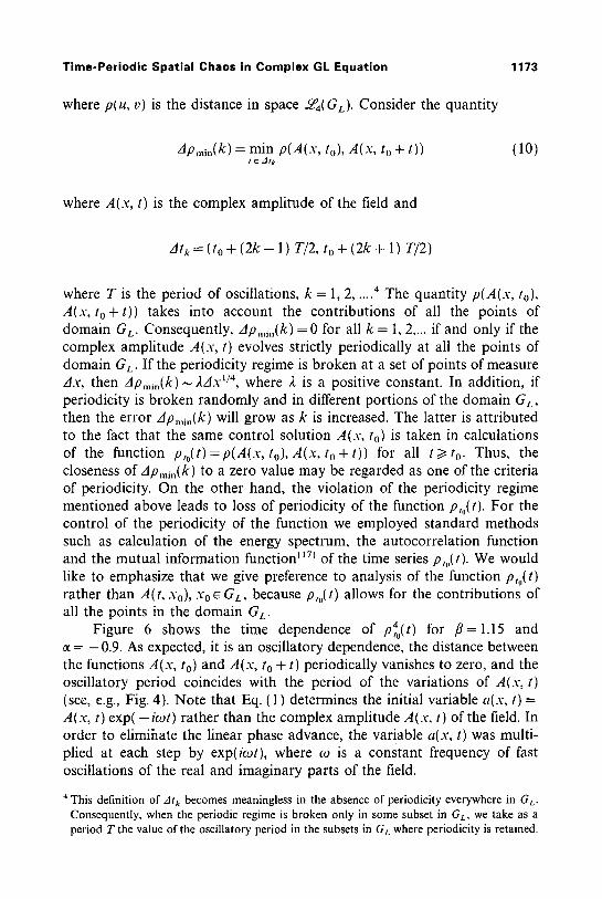
where p(u, v) is the distance in space L, e4(GL). Consider the quantity

Apmi,(k) = min p(A(x, to), A(x, t o + t)) (10) t ~ ZItk

where A(x, t) is the complex amplitude of the field and

A t ~=( t0+ ( 2 k - 1) T/2, t o + ( 2 k + 1) T/2)

where T is the period of oscillations, k = 1, 2 ..... 4 The quantity p(A(x, to), A(x, to+t)) takes into account the contributions of all the points of domain GL. Consequently, APmin(k) = 0 for all k = 1, 2 .... if and only if the complex amplitude A(x, t) evolves strictly periodically at all the points of domain GL. If the periodicity regime is broken at a set of points of measure zJx, then Apmin(k)--~ 2Ax ~/4, where 2 is a positive constant. In addition, if periodicity is broken randomly and in different portions of the domain GL, then the error APn, in(k) will grow as k is increased. The latter is attributed to the fact that the same control solution A(x, to) is taken in calculations of the function p,o(t) =p(A(x, to), A(x, to + t)) for all t >~ to. Thus, the closeness of Apmi.(k ) to a zero value may be regarded as one of the criteria of periodicity. On the other hand, the violation of the periodicity regime mentioned above leads to loss of periodicity of the function p,o(t). For the control of the periodicity of the function we employed standard methods such as calculation of the energy spectrum, the autocorrelation function and the mutual information function 117) of the time series p,,,(t). We would like to emphasize that we give preference to analysis of the function p,o(t) rather than A(t, Xo), Xo~ Gz., because p,o(t) allows for the contributions of all the points in the domain GL.

4 t Figure 6 shows the time dependence of p,0() for f l= l .15 and 0c = -0.9. As expected, it is an oscillatory dependence, the distance between the functions A(x, to) and A(x, to + t) periodically vanishes to zero, and the oscillatory period coincides with the period of the variations of A(x, t) (see, e.g., Fig. 4). Note that Eq. ( 1 ) determines the initial variable a(x, t) = A(x, t) e x p ( - icot) rather than the complex amplitude A(x, t) of the field. In order to elimihate the linear phase advance, the variable a(x, t) was multi- plied at each step by exp(icot), where 09 is a constant frequency of fast oscillations of the real and imaginary parts of the field.

4 Tiffs definition of A t k becomes meaningless in the absence of periodicity everywhere in GL. Consequently, when the periodic regime is broken only in some subset in GL, we take as a period T the value of the oscillatory period in the subsets in GL where periodicity is retained.

1174 Bazhenov et al.

Fig. 6.

10

0 26000

/0 4

26050 i l l i i

26100 TIME

l l l J , J l l I I D I ~ 1 1

26150 26200

Distance p4(A(x, to), A(x, to+ t)) versus time for /~= 1.15 and ~ = --0.9. The function p4 oscillates in time with period T ~ 4 3 .

The value of r found in experiments always has an error of A(o. The corresponding error in calculating p,u(t) will build up with increasing t, which will inevitably give Apmin(k) > 0 at sufficiently large times even if the solution of interest is strictly periodic at all points. Therefore for the control of the periodicity of the solution a(x, t) at large time intervals it is expedient to consider p(,~l(t) = p(la(x, to)l, [a(x, to + t)[). The function p(,~)(t) has the sense of the distance between the field amplitudes and does not take into account directly the phases of the compared functions. However, a(x, t) and a(x, to + t) are not arbitrary functions; instead, they are solutions of Eq. (1) and there is a definite relationship between their amplitude and phase. In the case of small-amplitude fluctuations (e.g., in the region between the neighboring hole solutions), this relationship may be represented as an algebraic dependence of field amplitude on its phase (see, e.g., ref. 2). Thus, periodic behavior of the function p(,~)(t) should also indicate the periodicity of the phase of complex amplitude A(x, t). This, however, is not a rigorous statement. In the general case, the field amplitude la(x, t)l may change periodically in time, while the phase arg(a(x, t)) does not change periodically. In this case, the function (1) P,o (t) is periodic and p,0(t) is nonperiodic. Thus, periodicity of the function (~) P,o (t) attests, strictly speaking, only to time periodicity of the field amplitude la(x, t)l [or IA(x, t)[]. We will use the quantity (~) P,0 (t) [it can be calculated more accurately than p,0(t)] for investigation of the transition from time- periodic spatial disorder to chaos as the parameters are changed.

Figure 7 shows as an example results of calculations of the energy spectrum and autocorrelation function for p(,~ i(t) at fl = 1.15 and ~ = - 0.8 for 2L=2000. These results indicate that p(,~)(t) changes periodically in time. Close analysis of the behavior of the function p(,~)(t) at large times > 1000T (where T is the oscillatory period) reveals an increase of AptS,(k)

Time-Periodic Spatial Chaos in Complex GL Equation 1175

K 300-

280

260

240

7- 2 2 0

0 100 200 300

(a)

~ 5-

0 0.0

(b)

I , [ L, L , ~ ,

o . ' s ' 1.b ' ' I . ' 5

Fig. 7. (a) Autocorrelation function K(r) and (b) energy spectrum S((2) (the zero harmonic is not indicated in the figure) calculated for p~,~ ~(t) at fl = 1.15, ~ = -0 .8 , and 2L = 2000. The calculations were performed in the time interval 12007", where T ~ 4 2 is the oscillatory period.

as k grows. 5 This indicates, as ment ioned above, that the periodici ty regime is b roken at some points. However , I~ Apm~,(k) increases ra ther slowly, for example, I 1 ~ ~1 APmin(k)/Apm~(k) < 0.05 for k ~ 1000, fl = 1.15, and ~ = - 0 . 8 . Thus the process is periodic at each t ime instant nearly at all points in the domain GL, except a set of small but nonzero measure Ax(Ax/2L ,~ 1). In this sense we "refer to the solutions as periodic everywhere in this paper.

The measure of the set of points for which there is no periodici ty increases with decreasing distance to the bounda ry of periodici ty domain

5 The function zlpmi.(k ) increases with the increase of k analogously. Figure 6 depicts the first four minima of the function p(t) only, but its analysis at large times attest to slow increase of ~Pmin(k ).

1 1 7 6 B a z h e n o v et al.

(see Fig. 1). Figure 8 gives a plot of A "(1) '1) versus cc for f l= 1.15. For - - p ' r a i n q .

c~>~ 1 we have I~ - Apm~.(l)<0.05, which indicates that the periodicity condition is met almost at all the points of domain GL. Starting from c (= -1 .025 , the value of Ap~i~(1) grows sharply and Aphid(I )~ Ap~,~x(1) ~ 50. The latter means total breaking of periodicity.

A spatiotemporal plot of the real part of the field is given in Fig. 9 for f l= 1.15 and ~ = -- 1.06. Note that, although the value of Apmin(I;~ 1 ) of about 27.4 indicates that the periodicity is broken at many points, on the whole the x versus t plots still looks like a periodic one.

The function p~,~(t) is essentially nonperiodic, has no pronounced maxima, and has a continuous energy spectrum with decaying mutual information function at the points that are referred to the region of spatiotemporal chaos in Fig. I. In addition, its correlation dimension is much greater than unity. All this indicates that A(x, t) has a complicated chaotic behavior in time for all or nearly all points in the domain GL.

The oscillatory period T of the field amplitude for the parameters from the periodicity domain is invariant to initial conditions. The time dependence of the distance between functions A(x, t o) and A'(x, to+t) corresponding to different (chaotic) initial conditions (a(x, 0) and a'(x, 0)) is shown in Fig. 10. It is well seen that this dependence is periodic, although the distance p(A(x, to), A'(x, to + t)) does not vanish to zero. The

, , ( 1 ) /

60" / - " ~ P m i n ~ 1 )

50"

40-

30"

20"

10"

�9

0 , , , ,1 . . . . I ,,', , I , , ' . . . . . . ; 0.8 0.9 1.0 1.1 1.2 1.3

Fig. 8. ApI,,l~i~(1) v e r s u s cc for fl= 1.15. In passing across the boundary of the periodicity domain, Ap~i~.(1) grows from ~0.05 (periodicity occurs ahnost everywhere) to ~50 (no periodicity).

Time-Periodic Spatial Chaos in Complex GL Equation 1177

Fig. 9. Spatiotemporal plot of the real part of the field for f l = l . 1 5 and c t = - l , 0 6 . Periodicity is broken at many points of domain Go.

latter may be caused by a constant phase difference of the oscillations A(x, t) and A'(x, t). Indeed, let a'(x, t )=a(x , t)exp(icp). Then

p(A(x, to), A(x, to + t) e ~~

=( fo [ tA(x, + IA(-,, 'o+')t 2 L

- 2 Re(A(x, to) ,4(x, t o + t) e-i*')] "- dx ) t/4 (11)

Fig. 10.

10- p 4

0 ; ~ I t i i q q i i I I J t t I ~ [ I J l t l I I I ~ l , I * t t ~ I I I I I I i i

26000 26050 26100 26150 26200 TIME

The same as in Fig. 6, but for spatial distributions corresponding to different initial conditions,

1178 Bazhenov e t al.

where ~0 is a constant value. If at the time instant t = T we have A(x, to) = A(x, to + T), then

p(A(x, to), A(x, to + T) e i~)

= [ 2 ( 1 - cos ~o ) ] ' /2 [ ~oL 114

IA(x, t0)] 4 dx (12)

Clearly, the expression (12) is not equal to zero if ~0 4: 2rtn, n =0, ___1 .....

4. STRUCTURAL STABILITY OF PERIODICITY REGIME

The results obtained indicate that the regime of time-periodic spatial disorder is stable and is realized at arbitrary initial conditions corresponding to the basin of attraction of a large-amplitude attractor (see Section 2). However, the problem of structural stability of this regime, i.e., of stability with respect to small perturbations of the right-hand side of Eq. (1), is unclear. In this connection we would like to recall ref. 12, in which the structural stability of hole solutions was investigated and it was shown that perturbations of the form + dlal4a, 6 ~ 1, may either reinforce or break the stability of such solutions, depending on their sign. Following ref. 12, we investigated the stability of the periodic regime of interest with respect to perturbations of the right-hand side of the equation of the form +d la] 4 a (where d ~ 0.0005 and ,,It ~ 0.01 is the integration step). It was found that the temporally periodic regime is structurally stable in all the considered cases. The period of oscillations is a continuous function of the right-hand side of Eq. (1), although the shape of the oscillation varies significantly with the change of the sign of perturbation.

Results of numerical simulation of a 2D CGLE also confirm the struc- tural stability of the regime of time-periodic spatial disorder considered above. We investigated a region in the form of a narrow strip L.,. x Ly(L,. ~>L;.) with periodic boundary conditions in both directions. The regime of spatiotemporal chaos that is inhomogeneous in both directions was chosen as initial conditions. We set •= 1.15 and investigated two cases: L x = 600 and L.,. = 1000 for different values of ~. It was found that, for the strip width smaller than the critical value (L~.r~29), a regime of time-periodic spatial disorder is established in the system for the values of the parameters from the periodicity region (see Fig. 1). The oscillatory period does not depend on L,. and coincides with the corresponding period found for the 1D CGLE. The field persists to be chaotic only along the x axis and is homogeneous along the 3' axis. Thus, the regime of time-periodic spatial disorder for the 2D CGLE is actually quasi-one-dimensional. The latter circumstance explains the coincidence of the oscillatory periods and

Time-Periodic Spatial Chaos in Complex GL Equation 1179

periodicity domains for the 1D and 2D CGLE. If the width of the region exceeds L.,~, r, there is no time periodicity, and the regime of spatiotemporal chaos is retained in the system.

The periodic regime described above may result from the Hopf bifur- cation of a stable spatial distribution containing a family of holes. Such a scenario looks quite probable if we consider the system (1) as a chain of coupled oscillators. In this representation, such a regime may be inter- preted as the result of complete synchronization of the oscillators having different intensities and, consequently, different oscillatory frequencies. A similar regime of synchronization for a 2D CGLE was investigated in ref. 18.

5. D I S C U S S I O N

The results of computer experiment presented above indicate that there exists a limit cycle with a finite basin of attraction in the phase space of system (I). In the general case, the phase space may have a rather com- plicated organization and contains a family of periodic trajectories of equal periods. This is also confirmed by the fact that different oscillations may be self-excited in the system at different initial conditions. The period of oscillations is actually the only parameter invariant to the length of the system and to initial conditions.

Computer experiment shows that the transition from a periodic to a chaotic regime occurs via intermittency. The time needed for the periodic excitations to set in grows with decreasing distance to the boundary of the periodicity domain, and, starting from some values of the parameters, we fail to detect periodicity. The oscillations near the boundary are periodic at some points along the x coordinate and aperiodic at the others.

Analytical description of time-periodic spatial disorder is a difficult problem. We well employ temporal periodicity in order to obtain a family of ODEs describing spatial disorder. Taking into consideration that any periodic function of period T may be expanded in the Fourier series in a complete system of orthogonal T-periodic functions, we can represent the solution a(x, t) of Eq. (1) in the form

a(x, t )= Ak(x) ~k(t) e -i'~ (13) k = O

where {~b,(t)} is a complete system of orthogonal functions of period T. One need not necessarily write the term exp(-i~ot) in an explicit form, but such a representation is quite natural if one recalls that the spatially homogeneous solution to (1) has the form a( t )= exp(-icot).

1180 Bazhenov e t al.

An approximate solution to (1) can be written as a finite series

( m I a, , , (x , t )= ~ Ak(x) tpk(t) e -i~ (11) \ k = 0

Since the solution (14) is not an exact solution of Eq. ( 1 ), the difference

Oa,,, ~ " F(a,,,) - ~ - - a , , , + (l + ifl) [a,,,[- a , , , - ( l + ioO O-a'' = Ox 2 (15)

cannot be identical to zero. Hence there arises the problem of minimizing, in a certain sense, this difference by choosing an appropriate function A t ( x ) ( k = 0 ..... m).

By using the Galerkin method, we find a system of ordinary differential equations (ODE) for the variables A~.(x):

T ( m / I_ Fk E At(x)I~k(t)e-i'~ ~s (/) ei~ dt=O, s = 0 ..... m (16)

\k=O

where ~ is a complex conjugate of ~. The function a,,,(x, t) is not an exact solution of (1), but it can be

represented as an exact solution of a reduced system aa,,,/at =Lm(S(a, , , )) , where S is the operator from the right-hand side of (1) and L,, is the operator of truncation of the Fourier series.

In passing from the series (13) to the finite series (14) the choice of a system of orthogonal T-periodic functions { ~bk(t) } becomes of fundamental significance. The system of functions of the form qJk(t)=exp(++_ikg2t), E2 = 2 n / T that is acceptable in many cases is not quite suitable here because the real oscillations observed in the system differ strongly from the harmonic ones (see Figs. 4 and 5) and a great number of harmonics must be taken into account for adequate description of the behavior of the system. Nevertheless, we can assert that for any time-periodic solution a(x, t) of Eq. (1) there exist a Galerkin approximation of a sufficiently high order which approximates this solution with preset accuracy. The approximate solution a,,,(x, t) at each fixed instant of time is described by a finite-dimensional ODE system. Consequently, at each time instant t = t 0, the spatial field distribution a(x, to) observed in numerical experiment is approximated to arbitrary accuracy by the solution of a finite-dimensional dynamical system (along x) for a,,(x, to). However, it is still to be found whether the exact solution a(x, to) is finite-dimensional.

The considerations presented on the origin of the observed phenomenon are confirmed by recent results obtained in ref. 19, where an extended system in the form of a "one-way coupled logistic lattice" was

Time-Periodic Spatial Chaos in Complex GL Equation 1181

investigated. It was revealed that spatial chaos with temporal periodicity may stably exist in a broad region of parameters, in particular, at sufficiently strong coupling. Such a regime appears to be quite natural in terms of the synchronization phenomenon since the medium is discrete and unidirectional. In this case, however, forced synchronization occurs instead of mutual synchronization of structures (or oscillators) because the coupling in the chain is unidirectional, whereas the spatial disorder is determined by the difference of intensity pulsations in each element of the chain.

AC KNOWLE DG M ENTS

This paper was made possible in part thanks to the Russian Foundation for Basic Research (project code N 94-02-03263-a) and the International Science Foundation (grant N NOU 000). M.B. highly appreciates the hospitality of the Niels Bohr Institute, where he performed part of the research described in this paper. L. R. is grateful to the International Soros Science Education Program, which awarded him a Soros Student Grant.

REFERENCES

1. M. V. Bazhenov, M. I. Rabinovich, and A. L. Fabrikant, In Proceedings of the KIT hlter- national Workshop on the Physics of Pattern Formation hi Complex Dissipative Systems, S. Kai, ed. (World Scientific, Singapore, 1992), p. 361.

2. Y. Kuramoto, Chemical Oscillations, Waves, and Turbulence, (Springer-Verlag, Berlin, 1984).

3. A. S. Newell, Lect. Appl. Math. 15:157 (1974). 4. H. Sakaguchi, Prog. Theor. Phys. 84:792 (1990). 5. L. Gill, Nonlinearity 4:1213 (1991). 6. B. I. Shraiman, A. Pumir, W. Saarloos, P. C. Hohenberg, H. Chate, and M. Holen,

Physica D 57:241 (1992). 7. M. V. Bazhenov, M. I. Rabinovich, and A. L. Fabrikant, Phys. Lett. A 163:87 (1992). 8. H. Chate, Nonlflmarity 7:185 (1994). 9. M. C. Cross and P. C. Hohenberg, Rev. Mod. Phys. 65(3):851 (1993).

10. K. Nozaki and N. Bekki, J. Phys. Soc. Jpn. 53:1581 (1984). 11. P. S. Hagan, SIAM J. Appl. Math. 42:762 (1982). 12. I. Aranson, L. Kramer, S. Popp, O. Stiller, and A. Weber, Phys. Ret,. Lett. 70:3880 (1993). 13. A. Weber, L. Kramer, I. S. Aranson, and L. Aranson, Phys. Rev. A 46:R2992 (1992). 14. H. Sakaguchi, Prog. Theor. Phys. 85:417 (1991). 15. I. Aranson, L. Kramer, and A. Weber, Phys. Rev. Lett. 72:2316 (1994). 16. S. A. Orszag, Stud. Appl. Math. 20:293 (1971). C. Canuto, M..J. Hussaini, A. Quarteroni,

and T. A. Zand, Spectral Methods fit Fhdd Dynamics (Springer, Berlin, 1988). 17. A. M. Fraser and H. L. Swinney, Phys. Rev. A 33:1134 (1986). 18. M. Bazhenov and M. Rabinovich, Physica D 73:318 (1994). 19. F. H. Willeboordse and K. Kaneko, Phys. Rev. Lett. 73:533 (1994).

822/83/5-6-25