Embed Size (px)
Citation preview

Time Resolved Laser Induced Incandescence Analysis of Metal Aerosols
by
Nigel Roshan Singh
A thesis
presented to the University of Waterloo
in fulfillment of the
thesis requirement for the degree of
Master of Applied Science
in
Mechanical and Mechatronics Engineering (Nanotechnology)
Waterloo, Ontario, Canada, 2016
© Nigel Roshan Singh 2016

ii
Author’s Declaration
I hereby declare that I am the sole author of this thesis. This is a true copy of the thesis, including any
required final revisions, as accepted by my examiners.
I understand that my thesis may be made electronically available to the public.
iii
Abstract
Synthetic nanoparticles are finding widespread adoption in a growing number of commercial and
research applications. Their size dependent properties offer researchers a variety of ranging including
targeted drug delivery, catalysis, and environmental remediation. As these materials are being adopted
into these applications, there is a pressing need for a diagnostic which allows the accurate real time
measurement of the particle size since the functionality of the nanoparticles are size dependent. Time-
resolved laser-induced incandescence (TiRe-LII) is an in situ technique which allows the non-destructive
inference of the nanoparticle size in real time. This technique was developed as a particle size diagnostic
for soot primary particles and has been modified to characterize synthetic nanoparticles. The aerosolized
nanoparticles are heated with a laser pulse to its incandescence temperature and the incandescence is
measured as the nanoparticles are allowed to thermally equilibrate with the surrounding gas. As
nanoparticles of different sizes will cool at different rates, the nanoparticle size can be inferred by
modeling the incandescence using a spectroscopic and heat transfer model.
The present work summarizes experiments conducted on aerosolized iron, silver, and
molybdenum nanoparticles using TiRe-LII analysis. This includes the spectroscopic and heat transfer
models, TiRe-LII instrument calibration and operating conditions, the nanoparticle preparation,
comparisons of the TiRe-LII derived particle sizes to existing ex situ techniques, and the associated error
analysis. The models required to interpret the TiRe-LII data, the spectroscopic and heat transfer models,
are presented with the optical and physical parameters to solve them, as well as simulate the expected
heat transfer modes of each of the nanoparticles. The calibration of the apparatus used as well as the
nanoparticle preparation, and TiRe-LII experimental measurement methods are discussed, as well as the
error bounds on the results.
A fluence study was conducted by looking at the peak temperatures measured as a function of
the fluence of the TiRe-LII instrument laser to determine the accuracy of the optical properties and to
compare the results to the trends to previous studies. The nanoparticle size and thermal accommodation
coefficient (TAC) of each of the aerosolized nanoparticle mixtures were attempted to be recovered based
on the heat transfer modes present in the TiRe-LII measurements. The aerosolized iron nanoparticles had
sufficient evaporation and conduction heat transfer modes which allowed the recovery of both the
nanoparticle size and thermal accommodations coefficient, while the aerosolized silver nanoparticles only

iv
had heat transfer due to evaporation which only allowed the recovery of the nanoparticle size, and the
aerosolized molybdenum nanoparticles only had heat transfer due to conduction which only allowed the
recovery of the nanoparticle size to TAC ratio. The molybdenum TAC was recovered by introducing the ex
situ calculated molybdenum nanoparticle size and nanoparticle size distribution, using electron
microscopy, into the models. Finally, the error bounds for the TiRe-LII measurements are presented, and
a perturbation analysis was performed due to the lack of provided error bounds on the optical and
physical properties used. It was shown that the optical properties had a significant impact on the
recovered nanoparticle size and TAC for all of the materials, while there was a lesser but non-trivial impact
on the recovered values from the nanomaterials’ physical properties.

v
Acknowledgements
I would like to thank my supervisor Dr. Kyle Daun for giving me the opportunity to become
involved in an exciting research field. I would like to thank him for his support and understanding
throughout the study.
I would like to thank the collaborators who have also helped me with the technical aspects
throughout this study. I would like to thank Mr. Navid Bizmark for his assistance with the iron nanoparticle
experiments, Mr. Robert Liang for his assistance with the silver nanoparticle experiments and Mr. Andrew
Kacheff for his valuable insight on the ex situ analysis. I would like to thank Dr. Zhongchao and Raheleh
Givehchi for access and their assistance with the TSI atomizer system.
I would like to thank my readers Dr. Kyle Daun, Dr. Ehsan Toyserkani, and Dr. Zhongchao Tan for
their time and insight for reviewing this study.
Finally, I would like to thank my family, colleagues from the Radiative Heat Transfer group
(including Josh Rasera, Noel Chester, Kamal Jhajj, Roger Tsang, Sam Grauer, Natalie Field, and Paul
Hadwin) for their assistance throughout the completion of this degree.

vi
Table of Contents
Author’s Declaration ..................................................................................................................................... ii
Abstract ........................................................................................................................................................ iii
Acknowledgements ....................................................................................................................................... v
Table of Contents ......................................................................................................................................... vi
List of Figures ............................................................................................................................................. viii
List of Tables ................................................................................................................................................. x
Nomenclature .............................................................................................................................................. xi
Chapter 1 Introduction ................................................................................................................................. 1
1.1 Motivation ........................................................................................................................................... 1
1.2 Background ......................................................................................................................................... 4
1.2.1 TiRe-LII studies on synthetic metal nanoparticles size characterization ..................................... 4
1.2.2 TiRe-LII studies on TAC ................................................................................................................. 6
1.3 Motivation of Present Work and Thesis Outline................................................................................. 7
Chapter 2 TiRe-LII Theory and Methods ..................................................................................................... 10
2.1 Spectroscopic Model ......................................................................................................................... 10
2.2 Nanoparticle Cooling Model ............................................................................................................. 12
2.3 Material Properties ........................................................................................................................... 15
2.3.1 Spectroscopic Properties ........................................................................................................... 15
2.3.2 Nanoparticle Cooling Properties ................................................................................................ 22
2.3 Nanoparticle Size and TAC Inference, and Uncertainty Quantification ............................................ 27
Chapter 3 Experimental Apparatus ............................................................................................................. 29
3.1 TiRe-LII Experimental Overview ........................................................................................................ 29
3.2 TiRe-LII Subsystem ............................................................................................................................ 31
3.3 TSI Atomizer Subsystem .................................................................................................................... 35
3.4 Ex Situ Characterization .................................................................................................................... 36
Chapter 4 Experimental Procedure............................................................................................................. 39
4.1 Nanoparticle Preparation .................................................................................................................. 39
4.1.2 Iron Nanoparticle Preparation ................................................................................................... 40
4.1.3 Silver Nanoparticle Preparation ................................................................................................. 41
4.1.4 Molybdenum Nanoparticle Preparation .................................................................................... 44
4.2 TiRe-LII Measurement Procedure ..................................................................................................... 46

vii
4.2.1 Preparation and Inspection ....................................................................................................... 46
4.2.2 Nanocolloid Synthesis and Setup ............................................................................................... 46
4.2.3 Activate TiRe-LII Apparatus ........................................................................................................ 46
4.2.3 Shut Down and Cleanup............................................................................................................. 47
4.3 Laboratory Safety .............................................................................................................................. 47
Chapter 5 Results ........................................................................................................................................ 48
5.1 Fluence and Spectroscopic Results ................................................................................................... 48
5.2 TiRe-LII Nanoparticle Size and TAC Analysis ..................................................................................... 55
5.2.1 Nanoparticle size and TAC recovery .............................................................................................. 55
5.2.2 Perturbation Analysis ..................................................................................................................... 64
Chapter 6 Conclusions and Future Work .................................................................................................... 67
References .................................................................................................................................................. 69

viii
List of Figures
Fig. 1 Magnetic response curves for iron oxide [3] ...................................................................................... 2
Fig. 2 Schematic of a TiRe-LII experimental measurement [22] ................................................................... 3
Fig. 3 Cooling curves for a simulated iron nanoparticle at different sizes.................................................... 4
Fig. 4 Experimental iron nanoparticle incandescence and calculated effective temperature. .................. 12
Fig. 5 Real and imaginary components of the refractive index for molten iron ......................................... 17
Fig. 6 E(m) values molten iron ................................................................................................................... 18
Fig. 7 Real and imaginary components of the refractive index for molten silver....................................... 19
Fig. 8 E(m) values molten silver ................................................................................................................. 20
Fig. 9 Real and imaginary components of the refractive index for molybdenum ...................................... 21
Fig. 10 E(m) values for molybdenum at different temperatures .............................................................. 22
Fig. 11 Heat transfer modes for a simulated iron nanoparticle.................................................................. 24
Fig. 12 Heat transfer modes for a simulated silver nanoparticle ............................................................... 25
Fig. 13 Heat transfer modes for a simulated molybdenum nanoparticle .................................................. 26
Fig. 14 Marginalization plot for a Fe-Ar aerosol ......................................................................................... 28
Fig. 15 Schematic of the TiRe-LII experimental apparatus [28]. ................................................................. 29
Fig. 16 Relative pressure changes during a TiRe-LII Experiment ................................................................ 31
Fig. 17 Beam profile results of a) the direct laser beam, and b) the laser beam passing through the ceramic
aperture and relay lens. ................................................................................................................. 32
Fig. 18 TiRe-LII Apparatus showing a) aperture and lens system, b) window 1, c) pyroelectric sensor ..... 33
Fig. 19 TiRe-LII Apparatus showing a) collection aperture wheel, b) density filter wheel, c) beam splitter
and the wavelength specific PMTs ................................................................................................ 34
Fig. 20 TSI atomizer subsystem, aerosolizing an iron nanocolloid ............................................................. 35
Fig. 21 Preparation of the TEM grids .......................................................................................................... 38
Fig. 22 Nanocolloids of: a) iron; b) silver; c) molybdenum ......................................................................... 40
Fig. 23 Sample TEM images of the iron nanoparticles, a) a larger nanoparticle showing the CMC coating,
b) a smaller nanoparticle. Scale bars corresponds to 50 nm in both images. ............................... 41
Fig. 24 Sample SEM image of the silver nanoparticles ............................................................................... 42
Fig. 25 Silver Nanoparticle SEM Histogram ................................................................................................ 43
Fig. 26 Sample TEM image of a molybdenum nanoparticle cluster ........................................................... 44
Fig. 27 Molybdenum Nanoparticle TEM Histogram ................................................................................... 45
ix
Fig. 28 Peak temperature vs fluence for iron nanoparticles ...................................................................... 50
Fig. 29 Comparison of the E(mlaser) from this study to the literature and Mie theory for iron ................. 51
Fig. 30 Peak temperature vs fluence for silver nanoparticles .................................................................... 52
Fig. 31 Peak temperature vs fluence for molybdenum nanoparticles ....................................................... 53
Fig. 32 Peak temperature vs fluence for silver nanoparticles for E(m)r = 0.366 and E(m)r = 1 .................. 54
Fig. 33 Plot of the experimental and modeled temperatures for the Fe-Ar aerosol .................................. 56
Fig. 34 Contour plot of the likelihood for the Fe-Ar aerosol ....................................................................... 57
Fig. 35 Iron nanoparticle colloid colour at: a) synthesis completion; b) one hour; c) six hours ................. 57
Fig. 36 Time evolution of the TAC for a Fe-Ar mixture during a TiRe-LII experiment ................................. 58
Fig. 37 Plot of the experimental and modeled temperatures for the Ag-Ar aerosol ................................. 60
Fig. 38 Contour plot of the likelihood for the Ag-Ar aerosol ...................................................................... 61
Fig. 39 Plot of the experimental and modeled temperatures for the Mo-Ar aerosol ................................ 63
Fig. 40 Contour plot of the likelihood for the Mo-Ar aerosol ..................................................................... 63
Fig. 41 Perturbation analysis results for the nanoparticle size (left) and TAC (right) for iron .................... 65
Fig. 42 (Left) Perturbation analysis results for the nanoparticle size for silver .......................................... 66
Fig. 43 (Right) Perturbation analysis results for the TAC for molybdenum ................................................ 66

x
List of Tables
Table 1 Nanoparticle Cooling Properties .................................................................................................... 23
Table 2 Laser Energy Measurements .......................................................................................................... 34
Table 3 Iron nanoparticle TiRe-LII size and TAC analysis ............................................................................ 56
Table 4 Silver nanoparticle TiRe-LII size analysis ........................................................................................ 60
Table 5 Molybdenum nanoparticle TiRe-LII TAC analysis using the TEM nanoparticle size ....................... 62
Table 6 Sensitivity analysis overview of parameters and perturbation factors ......................................... 64

xi
Nomenclature
Latin Symbols
Symbol Unit Definition
b - Observed data
C Pa Clausius-Clapeyron material constant
cg,t m·s-1 Mean thermal speed of gas molecules
cv,t m·s-1 Mean thermal speed of vapor molecules
c0 m·s-1 Speed of light in a vacuum, 3.00·108
cp J·kg-1·K-1 Specific heat capacity
cv m·s-1 Thermal speed of evaporating atoms
D m2·s-1 Diffusion coefficient
dp Nm Particle size
E J Energy
Ei J Pre-scattering energy of gas molecule
Eo J Post scattering energy of gas molecule
E(mλ) - Complex absorption function
h J·s Planck’s constant
Δhv J·atom-1 Enthalpy of vaporization
Δhv,b J·atom-1 Enthalpy of vaporization at the material boiling point
Ibλ W Blackbody radiation at wavelength λ
Jλ a.u. Incandescence at wavelength λ
K(dp,t) - Kernal of the incandescence equation
K J·atom-1 Material constant in Watson’s equation
kb J·mol-1·K-1 Boltzmann’s constant, 1.38·10-23
Kopt - Optical constant in the effective temperature equation
kλ - Imaginary component of the complex index of refraction
mg kg·mol-1 Molecular mass of a gas molecule
ms kg·atom-1 Mass of a surface atom
mv kg·atom-1 Mass of vapor atoms
Mv kg·mol-1 Molar mass of vapor

xii
mλ - Complex index of refraction
NA atoms·mol-1 Avogadro’s number
ng atoms·m-3 Gas number density
Ng atoms·s-1·m-2 Incident number flux of gas atoms
Nv atoms·s-1·m-2 Vapor molecular umber flux
nλ - Real component of complex index of refraction
P(b) - Evidence
P(b|x) - Likelihood
P(dp), P(dp,x) - Probability density of nanoparticles having size dp
P(x|b) - Posterior distribution
pg Pa Gas pressure
pg Pa Gas pressure
Ppr(x) - Prior distribution
pv Pa Vapor pressure
pv,o Pa Vapor pressure of bulk material
Qabs,λ(dp) - Absorption efficiency at wavelength λ
qcond W Conduction heat transfer
qevap W Evaporation heat transfer
qrad W Radiation heat transfer
R J·mol-1·K-1 Universal gas constant
RS J·kg-1·K-1 Specific gas constant
t ns Time
Tb K Boiling temperature
Tcr K Critical temperature
Teff K Effective temperature
Tg K Gas temperature
Tp K Particle temperature
Tp0 K Peak temperature
x - Size parameter
x - Vector of parameters of interest
xiii
Greek Symbols
Symbol Unit Definition
α - Thermal accommodation coefficient (TAC)
β - Collision efficiency
γs N·m-1 Surface tension of nanoparticle surface
λ nm Wavelength
ρ kg·m-3 Density
σj K, a.u. Standard deviation or noise in observed data
ζrot - Rotational degrees of freedom of a gas molecule
Subscripts
Subscript Definition
exp Experimental
g Gas
i Initial
i, j, k Indices
mod Modelled
o Out/final
p Particle
s Surface
v Vapor
Abbreviations
Abbreviation Definition
CMC Carboxymethyl cellulose
DLS Dynamic light scattering
MLE Maximum likelihood estimator
RSC Relative sensitivity coefficient
SEM Scanning electron microscopy
TEM Transmission electron microscopy
TiRe-LII Time-resolved laser-induced incandescence


1
Chapter 1 Introduction
1.1 Motivation
Synthetic metallic nanoparticles have found widespread adoption in a variety of disciplines due
to their unique size-dependent chemical and electromagnetic properties, many of which deviate from
their bulk counterparts. These properties have been integrated into applications that range from
environmental remediation, catalysis, optical devices, antimicrobial coatings, and chemical sensors [1].
For example, iron nanoparticles have been a potential material candidate in research for drug delivery,
environmental remediation, and catalytic processes [2], based on its size dependant magnetic properties.
The magnetic properties for iron oxide nanoparticles are demonstrated in the magnetic response curves
for particle sizes of 4-15 nm, shown in Fig. 1 [3], and this result has been incorporated into research
including medical contrast imaging materials [4] and catalysis [5]. Silver nanoparticles have been well
studied for their antimicrobial properties and have been considered as a promising candidate to combat
the evolution of antibiotic resistant bacteria [6].
It is critical that there are real time diagnostics available to provide information on whether the
nanoparticles are synthesized at the appropriate size for the desired material property or if there is an
underlying experimental issue. Gas phase synthesis is a preferred route for large scale production of
nanoparticles due to its ease with scaling up and mass production processes but a potential drawback of
these synthesis techniques is that there are limited real time diagnostics available to provide in situ
nanoparticle size and size distribution measurements to ensure the appropriate particle size or size range
are being synthesized for the intended application. While online ex situ methods, including scanning
mobility particle size characterization could provide this information, they are sometimes limited in the
aerosol applications they can be applied to due to probing restrictions. Offline ex situ methods, including
electron microscopy and surface characterization techniques such as and gas adsorption/desorption
characterization, are commonly utilized to determine the nanoparticle size and distribution
characteristics, and whether isolated nanoparticles or fractal aggregates of the primary particles are
present with the key drawbacks being this information is determined after the nanoparticle synthesis is
over, and can be time consuming.

2
Additionally, there is a demand for a diagnostic which can aid with assessing the potential impact
of synthetic nanoparticles on the environment and human health [1]. The health and safety concerns of
many nanomaterials are still not fully known as research into their impact on the environment and
organisms are limited, although there have been efforts to improve upon this knowledgebase as
nanomaterial usage increases. The literature available for iron nanoparticle toxicology has weakly
suggested that they have an adverse effects on animal cells, plant cells, and human cells [7]. Specifically,
human bronchial epithelium cells, a component of the respiratory system, were observed to die in the
presence of saline solutions with iron nanoparticles dissolved in them although there are only limited
studies on this topic [8, 9]. Research on the toxicology of silver nanoparticles have also suggested that for
oral exposure, such as in the case for aerosolized nanoparticles, the intestinal tract and liver are generally
the primary targets, although inflammation and accumulation of other organs has been observed [10].
The lack of information for silver nanoparticles is particularly concerning due to its widespread use in
-125
-75
-25
25
75
125
-10000 -8000 -6000 -4000 -2000 0 2000 4000 6000 8000 10000
M [
emu
/g]
H [Oe]
4 nm
6 nm
9 nm
15 nm
Fig. 1 Magnetic response curves for iron oxide nanoparticles at different particle sizes [3]

3
biological research and applications [1, 6, 11]. While there have been review papers identifying the health
concerns of iron and silver nanoparticle safety, or lack of research so far, there have been very limited
research on molybdenum nanoparticles as it has not seen as widespread adoption yet. While there is very
limited toxicology literature for molybdenum nanoparticles, they have been shown to reduce cellular
mitochondrial function and inducing cell plasma membrane leakage, causing irreversible cellular damage
[12].
Time-resolved laser-induced incandescence (TiRe-LII), a real time combustion diagnostic mainly
used for sizing soot primary particles [13, 14, 15], has been extended to measure synthetic zero-valent
metal nanoparticles including silver [16], iron [17, 18], molybdenum [19, 20] and silicon [21]. In a TiRe-LII
experiment, a laser pulse heats nanoparticles in a sample volume of an aerosol, and the spectral
incandescence is measured, usually at multiple wavelengths, as the aerosolized nanoparticles thermally
equilibrate with the carrier gas, shown schematically in Fig. 2 [22]. An instantaneous effective
temperature can be calculated from the measured incandescence data if the radiative properties of the
nanoparticles are known. Since smaller nanoparticles cool at a faster rate than larger ones, the
nanoparticle size distribution can be inferred by regressing the experimental effective temperature to
data generated with a heat transfer model. This model is influenced by parameters which include the
nanomaterial’s density, specific heat, radiative properties, and thermal accommodation coefficient (TAC,
0.0
0.2
0.4
0.6
0.8
1.0
0 10 20 30 40 50
J [a
.u.]
t [ns]
1064 nm Nd:YAG Laser
Detector (Jλ1
, Jλ2
)
Fig. 2 Schematic of a TiRe-LII experimental measurement [22]
4
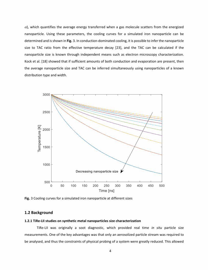
), which quantifies the average energy transferred when a gas molecule scatters from the energized
nanoparticle. Using these parameters, the cooling curves for a simulated iron nanoparticle can be
determined and is shown in Fig. 3. In conduction-dominated cooling, it is possible to infer the nanoparticle
size to TAC ratio from the effective temperature decay [23], and the TAC can be calculated if the
nanoparticle size is known through independent means such as electron microscopy characterization.
Kock et al. [18] showed that if sufficient amounts of both conduction and evaporation are present, then
the average nanoparticle size and TAC can be inferred simultaneously using nanoparticles of a known
distribution type and width.
Fig. 3 Cooling curves for a simulated iron nanoparticle at different sizes
1.2 Background
1.2.1 TiRe-LII studies on synthetic metal nanoparticles size characterization
TiRe-LII was originally a soot diagnostic, which provided real time in situ particle size
measurements. One of the key advantages was that only an aerosolized particle stream was required to
be analysed, and thus the constraints of physical probing of a system were greatly reduced. This allowed

5
TiRe-LII measurements to be performed in applications ranging from diesel internal combustion engine
[24] to larger aero-engines [25]. The sampling and size measurements of the aerosol during a TiRe-LII
experiment is within an enclosed environment since the laser module and the sample chamber are both
sealed, which is a significant advantage due to the potential health concerns of using nanoparticles.
While the heating of materials using laser pulses was not a novel concept, one the earliest
attempts to perform TiRe-LII size measurements on synthetic nanoparticles were by Vander Wal et al. in
1999 [26]. The study included TiRe-LII measurements on iron, molybdenum, titanium, and tungsten,
although the particle sizes were not recovered. This study did provide that in principle, the nanoparticle
size could be recovered if the nanoparticle cooling could be modelled accurately, which was still being
developed at the time.
An early attempt to recover the nanoparticle size was by Fillippov et al. [16], who studied ultrafine
silver, graphite, and titanium nitride nanoparticles. The nanoparticle size calculations from the TiRe-LII
measurements were erroneous as the conduction model used did not incorporate the temperature
dependent properties of the system, as well the study made the assumption that the thermal
accommodation coefficient was unity, which further research has suggested this value is not likely [27].
Furthermore, this study also reframed the determination of the nanoparticle size characteristics as solving
a Fredholm integral equation of the first kind, which is an inherently ill-posed problem but has many well
developed methods for solving and quantifying the error.
Murakami et al. [19] performed TiRe-LII measurements on molybdenum nanoparticles formed by
laser induced photolysis of Mo(CO)6 in different carrier gases. While the study was able to determine the
different aerosolized Mo nanoparticle sizes, there were several underlying issues with this study including:
the nanoparticles were assumed to be monodisperse while they are likely to be polydisperse; the study
utilised the heat transfer model from Filippov et al. [16] which made the assumption that the TAC was
unity; and material and gas properties used for the models were not temperature dependant. A reanalysis
of this study was conducted by Sipkens et al. [20] to address these deficiencies by implementing an
experimentally supported lognormal nanoparticle size distribution of g = 1.5 [18], implemented
temperature dependent properties, and attempted to recover the nanoparticle size and TAC instead of
assuming TAC = 1 and recovering only the nanoparticle size. This study showed that unlike materials such
as iron which have sufficient evaporation and conduction heat transfer modes which allow the

6
simultaneous determination of the nanoparticle size and TAC [18], the heat transfer of refractory
materials occur in the conduction only regime and the heat transfer model has the nanoparticle size and
TAC as a fixed ratio. To determine either the nanoparticle size or the TAC would require further ex situ
information, such as using electron microscopy to determine the nanoparticle size and then using that in
the model to determine the TAC.
1.2.2 TiRe-LII studies on TAC
To take into account of the TAC and how it influences TiRe-LII measurements, researchers started
determining the nanoparticle sizes from an alternative ex situ method, the preferred being transmission
electron microscopy (TEM), to determine the nanoparticle size and size distribution, and then using this
information to determine the material’s TAC. Kock et al. [18] utilised this method and attempted to
simultaneously recover the TAC and particle size from TiRe-LII measurements, based off of the lognormal
size distribution observed in TEM data of iron nanoparticles synthesized by the decomposition of Fe(CO)5
to iron nanoparticles using a hot wall reactor. It was found that the TAC was approximately 0.13 for iron
nanoparticles in both argon and nitrogen and the TiRe-LII particle sizes were consistent with the TEM
calculated sizes. The study also showed that from the TEM results, the iron nanoparticles synthesized in
argon were larger than the particles synthesized in nitrogen, which implied that the carrier gas may have
been influencing the synthesis. Similarly to Kock et al. [18], Eremin et al. [28] used both TiRe-LII and TEM
analysis to study iron nanoparticles formed by the photolysis of in argon, carbon monoxide, and helium
to study the effects of the carrier gas on the synthesis of the nanoparticles and how this affects the TiRe-
LII results. The study showed that the TAC for the iron nanoparticles changed depending on the carrier
gas used, specifically, 0.01 for helium, 0.1 for argon, and 0.2 for carbon monoxide, which supports the
claim that the direct comparison of TiRe-LII measurements from different studies is difficult since each
study is usually done using different experimental conditions.
An alternative method to calculate the TAC was proposed by Daun in 2009 [29] in which the TAC
was calculated using molecular dynamics simulations for interactions between soot and different gases,
including nitrogen, carbon monoxide, dinitrogen oxide, carbon dioxide, methane and ethane. The study
also showed that the molecular dynamics derived TAC values were consistent with the experimentally
derived TAC values. This work was extended to determine the nickel nanoparticle TAC values from both
molecular dynamics [30] and experimental data [31] but to date, accurate results have yet to be
determined.

7
While this study will focus on synthetic zero-valent metal nanoparticles, there have been further
TiRe-LII studies on metal oxides including MgO [32], TiO2 [33, 34], Fe2O3 [35], and SiO2 [36].
1.3 Motivation of Present Work and Thesis Outline
Recently, Sipkens et al. [37] successfully carried out TiRe-LII measurements on iron nanoparticles,
synthesized as a colloid and aerosolized using a pneumatic atomizer and is used as the starting point for
this study. By synthesizing the iron nanoparticles in solution and then aerosolizing with the carrier gas of
interest, the influence of the carrier gas on the synthesis of the nanoparticles is removed and allows the
TiRe-LII measurements of different aerosol mixtures to be compared directly. Some of the key limitations
of this study included: the observation of agglomeration and oxidation that occurred in solution, and
subsequent uncertainty regarding how these effects influenced TiRe-LII incandescence signals, the
experiments were limited to only iron nanoparticles and the effects of changing the laser fluence on the
temperatures observed was not investigated. Also, the iron nanoparticles only showed that this method
worked well when a sufficient amount of conduction and evaporation heat transfer is present in the
system, so the versatility materials which could also use this method is currently unexplored. This is one
of the key topics of investigation in this study by using silver which is expected to have heat transfer almost
entirely in the evaporation regime, and molybdenum which is expected to have heat transfer
predominately in the conduction regime.
The primary objectives of thesis is: to conduct TiRe-LII experiments using iron, silver, and
molybdenum nanoparticles, attempt to recover the nanoparticle size and TAC for different aerosolized
nanoparticle mixtures, determine the effects of changing the material properties used to interpret the
TiRe-LII signals, and to conduct a nanoparticle temperature study based on the laser fluence. Specifically,
this will be accomplished by building upon the experimental work of Sipkens et al. [37], starting with the
reanalysis and extension of the iron nanoparticle work including a temperature and fluence study, as well
as conducting the same experiments and analysis using silver and molybdenum nanoparticles.
Experimental TiRe-LII measurements are performed on aerosolized iron, silver, and molybdenum
nanoparticles using different carrier gases. In contrast to iron nanoparticles, silver colloids are known to
be stable in solution [1] and this also expected to be the same result for molybdenum. Colloidal solutions
of the respective nanoparticles are synthesized, aerosolized with a pneumatic atomizer using Ar, N2, and
CO2 as the carrier gases, and dried by flowing the mixture through a column of silica gel desiccant prior to
8
TiRe-LII measurement following the same procedure carried out by Sipkens et al. [37] on iron
nanoparticles. The spectral incandescence is measured at two wavelengths, and used to calculate an
effective temperature. The effects of changing laser fluence and candidate radiative properties for the
nanoparticles on the peak observed effective temperature are explored and how these changes affect the
absorption cross-section of the nanoparticles. Then heat transfer model is used to simultaneously infer
both the nanoparticle size and the TAC similarly to Sipkens et al. [37] by regressing data generated with a
heat transfer model to experimental data.
Chapter 2 provides an overview of the spectroscopic and heat transfer models, and the optical
and physical properties of the nanomaterials required to utilise these models. Specifically, the equations
used to model the incandescence, calculate the effective temperature, as well as the heat transfer mode
equations for evaporation, conduction, and radiation are presented.
Chapter 3 provides an overview of the TiRe-LII experimental apparatus required for nanoparticle
size measurements, and then further details each of the specific subsystems: the TiRe-LII subsystem and
the atomizer subsystem. A brief overview on the theory and principle of the ex situ analysis performed on
the nanoparticles in this study is also provided.
Chapter 4 discusses the synthesis methods used to prepare the nanoparticle colloids for iron,
silver, and molybdenum. The ex situ nanoparticle size and nanoparticle size distribution characterization
results from electron microscopy and dynamic light scattering are discussed. Also, the TiRe-LII
measurement procedure is also provided, including detailed steps on how the instruments are used and
the results are recorded.
Chapter 5 presents the results of the TiRe-LII measurements, as well as the fluence and peak
temperature analysis, and a comparison of the modelled spectroscopic properties to the experimentally
approximated counterparts. For iron, both the TAC and nanoparticle size could be recovered due to their
being sufficient evaporation and conduction, while the nanoparticle size could only be recovered for silver
due there only being evaporation, and only the nanoparticle size to TAC ratio could be recovered.

9
Chapter 6 summarizes the conclusions of the study and then provides recommendations for
future experiments. Specifically, further experiments which utilize credible optical and physical material
properties should be conducted.

10
Chapter 2 TiRe-LII Theory and Methods
To infer the nanoparticle size and TAC, the measured incandescence signals from a TiRe-LII
experiment are used to derive an instantaneous effective temperature, which can then be regressed with
simulated data from a heat transfer model. From this regression, an optimal nanoparticle size and TAC
pair is recovered that best reproduces the experimental data. In this chapter, the equations that are used
for the interpretation of a TiRe-LII analysis are discussed. Specifically, the spectroscopic and nanoparticle
cooling models, are introduced along with their governing equations. The statistical framework for
recovering the nanoparticle size and TAC values is presented and lastly, the TiRe-LII instrument setup and
calibration procedures are outlined.
2.1 Spectroscopic Model
The incandescence signals recorded during the TiRe-LII measurement is due to the emission from
all nanoparticle size classes that are present in the aerosol. At any instant, the spectral incandescence of
the laser-energized nanoparticles can be modeled by
0
, ,) )( ) ( ( ( , [ ( , ] () ) )p c p abs p b p p pJ t C P d d dA TQ I t d d d
(1)
where C is an instrument constant which accounts for the nanoparticle volume fraction, as well as the
collection optics geometry and photoelectric efficiency of the detectors, dp is the nanoparticle diameter,
P(dp) is the nanoparticle size distribution, Ac(dp) = dp2/4 is the cross-sectional area of the nanoparticle,
Qabs(dp,) is the spectral absorption efficiency at the detection wavelength, Ib,[(Tp(t,dp)] is the blackbody
intensity, and Tp is the nanoparticle temperature. Nanoparticles are expected to have diameters
sufficiently smaller than the detection wavelengths, the laser wavelength, and the mean free path of the
carrier gas. Consequently they emit and absorb radiation in the Rayleigh regime [38], so the absorption
efficiency is
2
, 2
14Im 4
2absQ x E x
mm
m (2)

11
where m = n + ik is the complex index of refraction, E(m) is the absorption function, and x = dp/ is
the size parameter.
Eq. (1) can be rewritten as a Fredholm integral equation of the first kind following the work by
Fillipov et al. [16]
0
) ( ,) ( ( ))( p p pK d tJ t P d d d
(3)
where all of the terms are grouped in the kernel, K(dp,t), excluding P(dp). The simulated incandescence values
depend on the size-dependent nanoparticle cooling curves, which in turn are calculated using a nanoparticle
cooling model discussed in Section 2.2. While dp could be inferred by solving Eq. (1) using incandescence
measured at a single wavelength, this procedure requires knowledge of C, which is generally not known.
Two-color (or auto-correlated) LII removes the dependence of C [39]; this procedure utilizes the spectral
incandescence measured at two wavelengths to derive an effective pyrometric temperature
1 2
2
16
0
B 2 1
1
1 2
( ) ( )1 1( ) ln
( ) ( )op
ft
e fp
J t EhcT t K
k J t E
m
m (4)
where h is Planck’s constant, c0 is the speed of light in a vacuum, kB is the Boltzmann constant, 1 and 2 are
the two detection wavelengths, Kopt = C1/C2 which the LII needs to be calibrated to account for, and
E(m2)/E(m1) is the ratio of the emission efficiencies at the detector wavelengths, also symbolized as E(m)r.
An example of TiRe-LII data is shown in Fig. 4 where the incandescence of cooling aerosolized iron
nanoparticles are measured at two wavelengths and then converted to the effective temperature.

12
From Eq. (4), calculating the effective temperature requires the ratio of the emission efficiencies at
the detector wavelengths, which by using Kirchhoff’s law, is equivalent to the spectral absorption efficiency,
defined in Eq. (2). For soot, E(m) is influenced by the fuel used and the combustion environment [38, 40],
while in nanoparticles of pure substances, the complex index of refraction should be a reasonable value to
use for the spectral absorption efficiency. This is may not work for all materials since the optical properties of
nanomaterials deviate from their bulk material properties due to the scattering of electrons [41]. Since there
are limited experimental sources which attempt to quantify this for solid high temperature and molten
nanoparticles, a dispersion model could be used instead to approximate E(m), and is discussed in Chapter 4.
2.2 Nanoparticle Cooling Model
Modeling the incandescence during nanoparticle cooling requires knowledge of Tp(dp,t), which can
be found by performing an energy balance on the energized nanoparticle as it thermally equilibrates with the
0
500
1000
1500
2000
2500
3000
3500
0.0E+00
2.0E+06
4.0E+06
6.0E+06
8.0E+06
1.0E+07
1.2E+07
0 50 100 150 200 250 300
Effe
ctiv
e Te
mp
erat
ure
[K
]
Inca
nd
esce
nce
[au
]
Time [ns]
J(442 nm)
J(716 nm)
Teff [K]
Fig. 4 Experimental iron nanoparticle incandescence and calculated effective temperature.

13
carrier gas. This energy balance sets the sensible energy equal to the nanoparticle heat transfer due to
conduction, evaporation and radiation, given by
3
, , ,6
p p
p p p cond p evap p rad p
dTq t d
dT c T qq t d t d
dt
(5)
where (Tp) and cp(Tp) are the temperature-dependent density and specific heat of the aerosolized
nanoparticle. Although radiation is the basis for the detection method, it has been shown to have a negligible
effect on the nanoparticle cooling model, when compared to the conduction and evaporation modes, and
will be omitted from the analysis [18].
The nanoparticle sizes are expected to be equal to or smaller than their mean-free path within the
carrier gas, so heat transfer occur in the free molecular regime. For example, Sipkens et al. [37] calculated the
mean-free path molecular path of CO2 to be approximately 40 nm, which is similar to the expected size range
of the nanoparticle used in the experiments. Free molecular heat conduction is given by
,2 " 2( , )4
g g t
cond p p g o i p o i
nd
cq t d E EN E d E (6)
where Ng is the incident gas number flux, ng = Pg/(kBTg) is the molecular number density of the carrier gas,
cg,t=[8kBTg/(mg)]1/2 is the mean thermal speed of the carrier gas, Pg, Tg, and mg are the carrier gas pressure,
temperature, and molecular mass, respectively, and EoEi is the average energy transfer per collision. The
latter term can be rewritten using the TAC, , which is defined as the ratio between the average energy
transfer and maximum energy transfer allowed by the Second Law of Thermodynamics
max2
2
roto i o i B p gE E kE E TT
(7)
where rot is the number of rotational degrees of freedom of the carrier gas. The monatomic gases have no
rotational modes available, so rot = 0, while the linear polyatomic gases requires rot = 2. The final form of the
heat transfer due to conduction is given by

14
,2( 24
)2
,g g t rot
cond p p p g
g
Pd T
T
cq t d T
(8)
with the appropriate value of rot used for the specific aerosolized nanoparticle mixture. The free molecular
evaporation is given by
2 " 2
4, v v
evap p v p v v p
nH d Nq t H
cd d (9)
where Hv is the heat of vaporization of the metal atoms, Nv is the vapor number flux, nv is the vapor number
density, cv is the mean thermal speed of the vapor and is the sticking coefficient. Following Sipkens et al.
[37], Hv is calculated using Watson’s equation [42]
0.38
/1v p cK T TH (10)
where K is a material constant which can be found by using the nanoparticle boiling temperature and enthalpy
of vaporization, and Tc is the critical temperature of the nanoparticle. Assuming that the molten nanoparticle
surface and its vapor above the surface are in quasi-equilibrium, the Clausius-Clapeyron equation can be used
to relate the heat of vaporization and the vapor pressure
,
1ln v
v o
p
HP C
R T
(11)
where R is the universal gas constant, and C is a material constant. Since this pressure value corresponds to a
flat interface between the two phases, this value can be further modified to account for the increased surface
energy due to nanoparticle curvature using the Kelvin equation [37]
, ex
4p
s
v v o
p s
p
pp
p pd
T
T TR
(12)
15
where Rs is the specific gas constant, and s(Tp) is the surface tension of the nanoparticle. The heat transfer
due to radiation is given by
,
2
,0
, [ ( , ), ]4
p
abs prad p b p p
dq t d Q TId t d d
(13)
where Qabs(dp,) is the spectral absorption efficiency at the detection wavelength, and Ib,[(Tp(t,dp),] is
the blackbody intensity. The spectral absorption efficiency corresponds to the incandescence calculated
for a single nanoparticle size and then integrated over all wavelengths to account for the total spectral
emission.
2.3 Material Properties
The material properties used for this analysis are presented for the spectroscopic and
nanoparticle cooling models. For the spectroscopic model, the results of the Drude model of the optical
properties are compared to the experimentally observed values reported in the literature, when possible.
The nanoparticle cooling model is then used to determine the influence of the fluence on the peak
temperatures for different aerosol mixtures, as well as to determine which heat transfer modes are
dominant.
2.3.1 Spectroscopic Properties
It is expected that for most materials considered in this study, the energized nanoparticles will exceed
their respective melting points [37], so the complex index of refraction for the molten nanoparticles should
be used when calculating E(m). There are only limited studies dedicated to quantifying the complex index
of refraction or their equivalent complex dielectric function = 1 + i2 of molten metals, and this work
utilizes the work previously published by Miller [43], Hodgson [44] and Krishnan et al. [45]. For some
metals, it may be possible to model the complex dielectric function using Drude theory [46, 47], in which
the kinetic motion of electrons are modeled as they collide with the metal’s heavier and immobile positive
ions. To model this, the complex dielectric components are given as
2 2
2 2
1 2 21
1
pn k
(14)

16
and
2
2 2 22
1
pnk
(15)
where = 2c0/ is the angular frequency of the E-M field, is the relaxation time (average time between
electron-ion and electron-neutral collisions), and p is the plasma frequency. The plasma frequency is
given by
*2 22
0
p
N e
m
(16)
where N* is the number of free electrons per unit volume, m and e are the mass and charge of an electron,
respectively, and 0 is the vacuum permittivity. Miller found that the effective carrier density N* is larger
than the density N of valence electrons, since the electron band structure above the Fermi level
disappears upon melting [43]. The relaxation time is found from the DC conductivity,
* 2
DC
N e
m
(17)
While there is interest in developing a Drude model for iron nanoparticles, a review of a previous study
by Sipkens et al. [37] revealed that the Drude parameters derived by Kobatake et al. [48] was shown to
be nonphysical and is not considered for this study. Instead, the experimentally derived spectroscopy
properties from Krishnan et al. [45], which are consistent with the values published by Miller [43], is used
in this study. The real and imaginary components of the refractive index of molten iron are shown in Fig.
5.

17
Fig. 5 Real and imaginary components of the refractive index for molten iron
The corresponding E(m) values are shown in Fig. 6, where vertical lines denote the E(m) values
at the laser wavelength used (1064 nm) and the two detection wavelengths, at 442 nm and 716 nm,
respectively. The experimental values from Krishnan et al. contained the required values for the detector
wavelengths of the TiRe-LII system, E(mnm) = 0.191 and E(mnm) = 0.103 respectively, but does not
include the laser wavelength, so a fourth order polynomial was fit (r2 = 0.9797) to the E(m) values from
Krishnan et al. [45] and extrapolated to find E(mnm) = 0.065, which is also shown in Fig. 6.
0.0
0.5
1.0
1.5
2.0
2.5
3.0
3.5
4.0
4.5
5.0
300 400 500 600 700 800 900 1000 1100
n, k
Wavelength [nm]
Krishnan n
Miller n
Krishnan k
Miller k

18
Fig. 6 E(m) values molten iron
For molten silver, the DC conductivity of 58.14103 (cm)1 and N*/N = 1.05 was used, following
Miller [43] and Krishnan et al. [45], resulting in p = 1.31751015 rad/s and = 3.782310-15 s. The real
and imaginary refractive indices obtained from Drude theory are plotted in Fig. 7.
0.00
0.02
0.04
0.06
0.08
0.10
0.12
0.14
0.16
0.18
0.20
300 400 500 600 700 800 900 1000 1100
E(m
)
wavelength [nm]
Krishnan
Krishnan (Quartic)
Miller

19
Fig. 7 Real and imaginary components of the refractive index for molten silver
The trends show good agreement with ellipsometry measurements on molten silver, which one would expect since the inter-band absorption structures present for solid metals do not exist in liquid state [43,
45, 49]. The corresponding E(m) values are plotted in Fig. 8
Fig. 8 E(m) values molten silver
. For this study the Drude derived E(m) values were selected to interpret the molten silver TiRe-LII data,
specifically, E(mnm) = 0.041 and E(mnm) = 0.015 and E(mnm) = 0.009.
0
1
2
3
4
5
6
7
8
300 400 500 600 700 800 900 1000 1100
n, k
Wavelength [nm]
Krishnan n
Miller n
Drude n
Krishnan k
Miller k
Drude k

20
Fig. 8 E(m) values molten silver
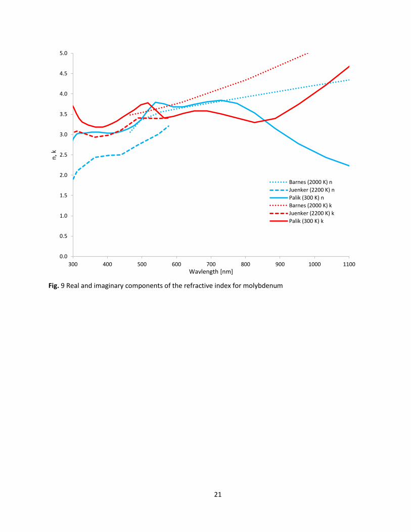
From preliminary trials it was observed that the TiRe-LII experiments on molybdenum
nanoparticles do not exceed its melting temperature (2896 K [50]), so high temperature solid state values
for the index of refraction were investigated. This is because the n, k and E(m) values depend on the
DC conductivity of the material which is directly influenced by the temperature through Drude/Hagen-
Rubens theory [38]. Experimental refractive index values were taken from Barnes on solid molybdenum
at 2000 K [51], Juenker et al. at 2200 K [52], and Palik et al. at 300 K [53] and are plotted in Fig. 9 with the
corresponding E(m) values plotted in Fig. 10. For this study the experimental E(m) values from Barnes
[51] were selected to interpret the molybdenum TiRe-LII data, specifically, E(mnm) = 0.151 and E(mnm)
= 0.097 and E(mnm) = 0.065.
0.00
0.02
0.04
0.06
0.08
0.10
0.12
0.14
0.16
0.18
0.20
300 400 500 600 700 800 900 1000 1100
E(m
)
Wavelength [nm]
Krishnan
Miller
Drude
21
Fig. 9 Real and imaginary components of the refractive index for molybdenum
0.0
0.5
1.0
1.5
2.0
2.5
3.0
3.5
4.0
4.5
5.0
300 400 500 600 700 800 900 1000 1100
n, k
Wavlength [nm]
Barnes (2000 K) n
Juenker (2200 K) n
Palik (300 K) n
Barnes (2000 K) k
Juenker (2200 K) k
Palik (300 K) k

22
Fig. 10 E(m) values for molybdenum at different temperatures
2.3.2 Nanoparticle Cooling Properties
To solve the nanoparticle cooling model outlined in section 2.2, the literature was surveyed for the
molten temperature dependent properties for iron and silver, and high temperature solid state values for
molybdenum. From preliminary tests, the peak TiRe-LII derived temperature of molybdenum nanoparticles
approaches but never exceeds its melting point, 2896 K [50], so it follows that high temperature solid state
values . Temperature dependent values could not be found for all the material properties, such as the surface
tension for molybdenum, and the next reasonable value found in the literature were used. All of the values
selected are summarized in
Table 1.
0.00
0.05
0.10
0.15
0.20
0.25
0.30
0.35
0.40
0.45
0.50
300 400 500 600 700 800 900 1000 1100
E(m
)
Wavelength [nm]
Barnes (2000 K)
Junker (2200 K)
Palik et al. (300 K)

23
Table 1 Nanoparticle Cooling Properties
a a(Tp) = (1582+0.0589·(Tp-Tm))·( 3.0+1.03·(10-3)·(Tp-Tm))
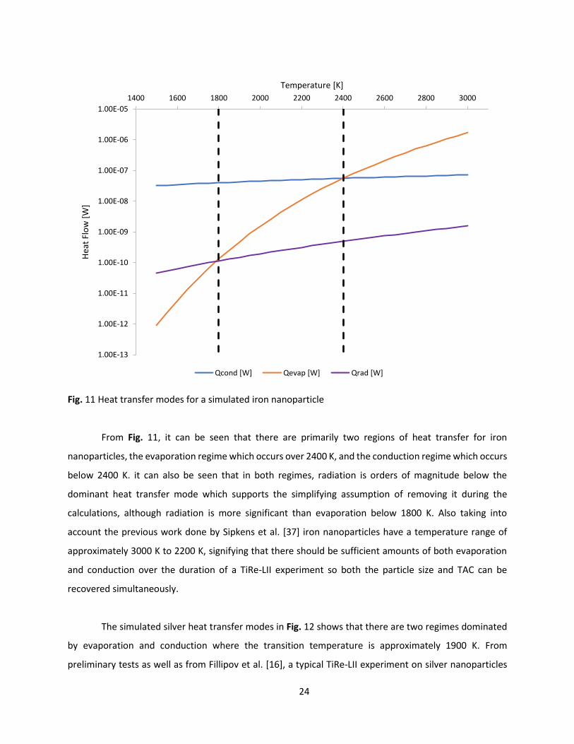
Using the physical properties listed in Table 1, Eq. (5) can be used to simulate nanoparticle cooling
data can be calculated and then used to approximate what kind of heat transfer modes should be
dominant as well as how we could modify our heat transfer model when using it to regress experimental
data to reduce our computational effort. Hypothetical 50 nm and 0.1 TAC iron, silver and molybdenum
nanoparticles were used to calculate the contribution of the conduction, evaporation and radiation heat
transfer modes between the expected TiRe-LII experiment temperature range of 1500 K to 3000 K, shown
in Fig. 11, Fig. 12, and Fig. 13 for iron, silver and molybdenum respectively.
Property Fe Ag Mo
mg [kg/mol] 0.05585 0.1080 0.9594
[kg/m3] 8171-0.64985·Tp [54] 9346-0.9067·(Tp-1234)
[55]
9100-0.6·(Tp-Tm), Tp>=Tm
9100-0.5·(Tp-Tm), Tp<Tm [50]
cp [J/(kg·K)] 835 [56] 531 [57] 56.5+0.01177·(Tp-Tm), Tp>=Tm
a(Tp)a, Tp<Tm [50]
Tm [K] 1811 [56] 1234 [55] 2896 [50]
Tb [K] 3134 [58] 2466 [59] 4913 [60]
Tcr [K] 9340 [61] 6410 [55] 14,588 [61]
Hv [J/mol] 340·(103) [58] 254·(103) [59] 582·(103) [62]
s [N/m] 1.865-(Tp-1823)·(0.35)·(10-3)
[63] 1.0994-0.0002·Tp [64] 2.11 [65]
24
Fig. 11 Heat transfer modes for a simulated iron nanoparticle
From Fig. 11, it can be seen that there are primarily two regions of heat transfer for iron
nanoparticles, the evaporation regime which occurs over 2400 K, and the conduction regime which occurs
below 2400 K. it can also be seen that in both regimes, radiation is orders of magnitude below the
dominant heat transfer mode which supports the simplifying assumption of removing it during the
calculations, although radiation is more significant than evaporation below 1800 K. Also taking into
account the previous work done by Sipkens et al. [37] iron nanoparticles have a temperature range of
approximately 3000 K to 2200 K, signifying that there should be sufficient amounts of both evaporation
and conduction over the duration of a TiRe-LII experiment so both the particle size and TAC can be
recovered simultaneously.
The simulated silver heat transfer modes in Fig. 12 shows that there are two regimes dominated
by evaporation and conduction where the transition temperature is approximately 1900 K. From
preliminary tests as well as from Fillipov et al. [16], a typical TiRe-LII experiment on silver nanoparticles
1.00E-13
1.00E-12
1.00E-11
1.00E-10
1.00E-09
1.00E-08
1.00E-07
1.00E-06
1.00E-05
1400 1600 1800 2000 2200 2400 2600 2800 3000
Hea
t Fl
ow
[W
]Temperature [K]
Qcond [W] Qevap [W] Qrad [W]

25
has a very short period of incandescence, approximately less than 100 ns which results in an approximate
temperature range from 2800 K to 2200 K. From these two observations, the assumption that TiRe-LII
experiments for silver predominantly occur in the evaporation only regime is supported so only the
nanoparticle size can be recovered since the evaporation model is not dependent on the TAC, which is
only required in the conduction model.
Fig. 12 Heat transfer modes for a simulated silver nanoparticle
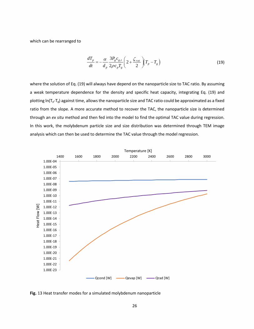
Lastly, the simulated molybdenum data in Fig. 13 clearly shows that the dominant heat transfer
mode for the entire TiRe-LII experiment range is conduction. This is consistent with previous studies work
done by Murakami et al. [19] and Sipkens et al. [20] where only the nanoparticle size and TAC ratio could
be determined due to molybdenum since Eq. (9) can be rewritten as,
3
,2 2,4 26
p p g g t rotp p p cond p p p g
g
dT cq t d T
d
d PT c T d T
Tt
(18)
1.00E-12
1.00E-11
1.00E-10
1.00E-09
1.00E-08
1.00E-07
1.00E-06
1.00E-05
1.00E-04
1400 1600 1800 2000 2200 2400 2600 2800 3000
Hea
t Fl
ow
[W
]
Temperature [K]
Qcond [W] Qevap [W] Qrad [W]
26
which can be rearranged to
,32
2 2
p g g t rotp g
p p g
PT
d
c
c T
dTT
dt
(19)
where the solution of Eq. (19) will always have depend on the nanoparticle size to TAC ratio. By assuming
a weak temperature dependence for the density and specific heat capacity, integrating Eq. (19) and
plotting ln(Tp-Tg) against time, allows the nanoparticle size and TAC ratio could be approximated as a fixed
ratio from the slope. A more accurate method to recover the TAC, the nanoparticle size is determined
through an ex situ method and then fed into the model to find the optimal TAC value during regression.
In this work, the molybdenum particle size and size distribution was determined through TEM image
analysis which can then be used to determine the TAC value through the model regression.
Fig. 13 Heat transfer modes for a simulated molybdenum nanoparticle
1.00E-23
1.00E-22
1.00E-21
1.00E-20
1.00E-19
1.00E-18
1.00E-17
1.00E-16
1.00E-15
1.00E-14
1.00E-13
1.00E-12
1.00E-11
1.00E-10
1.00E-09
1.00E-08
1.00E-07
1.00E-06
1.00E-05
1.00E-04
1400 1600 1800 2000 2200 2400 2600 2800 3000
Hea
t Fl
ow
[W
]
Temperature [K]
Qcond [W] Qevap [W] Qrad [W]
27
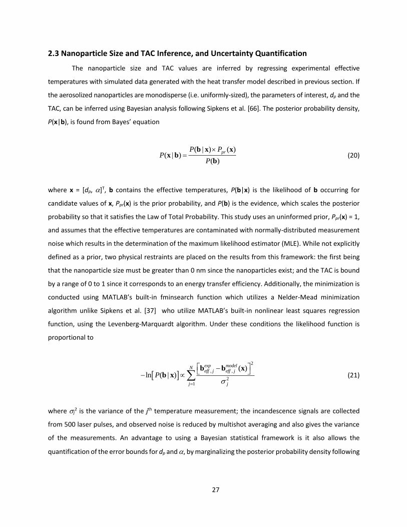
2.3 Nanoparticle Size and TAC Inference, and Uncertainty Quantification
The nanoparticle size and TAC values are inferred by regressing experimental effective
temperatures with simulated data generated with the heat transfer model described in previous section. If
the aerosolized nanoparticles are monodisperse (i.e. uniformly-sized), the parameters of interest, dp and the
TAC, can be inferred using Bayesian analysis following Sipkens et al. [66]. The posterior probability density,
P(x|b), is found from Bayes’ equation
( | ) ( )
( | )( )
prP PP
P
b x xx b
b (20)
where x = [dp, ]T, b contains the effective temperatures, P(b|x) is the likelihood of b occurring for
candidate values of x, Ppr(x) is the prior probability, and P(b) is the evidence, which scales the posterior
probability so that it satisfies the Law of Total Probability. This study uses an uninformed prior, Ppr(x) = 1,
and assumes that the effective temperatures are contaminated with normally-distributed measurement
noise which results in the determination of the maximum likelihood estimator (MLE). While not explicitly
defined as a prior, two physical restraints are placed on the results from this framework: the first being
that the nanoparticle size must be greater than 0 nm since the nanoparticles exist; and the TAC is bound
by a range of 0 to 1 since it corresponds to an energy transfer efficiency. Additionally, the minimization is
conducted using MATLAB’s built-in fminsearch function which utilizes a Nelder-Mead minimization
algorithm unlike Sipkens et al. [37] who utilize MATLAB’s built-in nonlinear least squares regression
function, using the Levenberg-Marquardt algorithm. Under these conditions the likelihood function is
proportional to
2
, ,
21
( )ln ( | )
exp modelNeff j eff j
j j
P
bx
b xb (21)
where j2 is the variance of the jth temperature measurement; the incandescence signals are collected
from 500 laser pulses, and observed noise is reduced by multishot averaging and also gives the variance
of the measurements. An advantage to using a Bayesian statistical framework is it also allows the
quantification of the error bounds for dp and , by marginalizing the posterior probability density following

28
Sipkens et al. [66], and an example of this is shown in Fig. 14, where the respective 95% error bounds are
shown as the filled in grey areas.
In addition to the quantification of the error bounds, there is an additional uncertainty assigned
to each of the nanoparticles’ physical properties as well as the operating conditions of the TiRe-LII
instrument which cannot easily be quantified. For this study, a perturbation analysis is performed for
some of the key physical parameters to determine the change, if any, from the recovered MLE solution.
Fig. 14 Marginalization plot for a Fe-Ar aerosol

29
Chapter 3 Experimental Apparatus
The TiRe-LII experimental apparatus is divided into two main subsystems: the TSI atomizer, which
is responsible for aerosolizing and drying the nanoparticles; and TiRe-LII instrument itself to laser heat the
nanoparticles and measure the incandescence. In this chapter, the operational parameters used in this
study are introduced for both subsystems. Furthermore, ex situ characterization techniques which were
used in conjunction with these subsystems, as they provide particle size measurements which can then
be compared to the TiRe-LII measurements, are also introduced and the discussed.
3.1 TiRe-LII Experimental Overview
This work uses an identical TiRe-LII experimental setup to Sipkens et al. [37] and a general
schematic is shown in entire process is depicted in Fig. 15, where the grey clusters represent the
nanoparticles, the blue clusters represent water molecules, the solid blue dots represent the carrier gas,
and the grey lines represent any residual materials from the synthesis procedure, including dispersants
and trace contaminants. In the case of the iron nanoparticles, a polymer layer is applied to the surface to
prevent the nanoparticles from oxidation and agglomeration which is assumed to be ablated during the laser
heating process, depicted as the grey lines being removed in the schematic in Fig. 15. The silver nanoparticles
use an aqueous dispersant to prevent nanoparticle agglomeration, which is removed during the aerosol
drying, while the molybdenum nanoparticles are not prepared with any dispersant.
Fig. 15 Schematic of the TiRe-LII experimental apparatus [37].

30
The TiRe-LII instrument is set up to allow an aerosolized mixture flow through the sample chamber
and then ventilated in a fume hood. When in operation, the system is completely closed which minimizes
the likelihood of the experimental area being exposed to nanoparticles. After the nanoparticles of interest
are made into a colloid, different aerosol mixtures are generated using a TSI Model 3076 pneumatic
atomizer operating in recirculation mode using the carrier gas of interest, at an inlet pressure of
approximately 200 kPa. This produces a stream of water droplets approximately 350 nm in diameter which
contains the nanoparticle of interest, any residual byproducts from the nanoparticle synthesis, and a
dispersing agent to prevent the nanoparticles from aggregating depending on the nanomaterial being
tested.
After aerosolization, the wet aerosol pass through a diffusion drier charged with a silica gel
desiccant, which removes any moisture from the aerosol. Since the residual byproducts and the dispersing
agents remain in liquid, they are also removed by the silica gel. The dried aerosol then reaches the TiRe-
LII sample chamber where the laser pulse heating occurs, and the incandescence is recorded as the
nanoparticles are allowed to thermally equilibrate with the carrier gas. The aerosolized nanoparticles
enter the sample chamber where the aerosol pressure is measured at 101.3 kPa ± 3.5 kPa using an Omega
PX409-USBH pressure transducer for the duration of a TiRe-LII experiment shown in Fig. 16, and is at room
temperature. From the schematic, the setup allows for an easy change of the motive gas which allows a
variety of different aerosol mixtures to be tested. While Sipkens et al. [37] previously utilized He, Ar, Ne,
CO, N2, CO2, and N2O for their TiRe-LII study on iron nanoparticles, this study limits the carrier gases to be
Ar, N2 and CO2.

31
Fig. 16 Relative pressure changes during a TiRe-LII Experiment
3.2 TiRe-LII Subsystem
The TiRe-LII experiment is carried out using an Artium 200 M system and was calibrated before this
study, under the supervision of Mr. Robert Sawchuk at the National Research Council of Canada. The
nanoparticles are energized using a 1064 nm Nd:YAG laser operating at 10 Hz. The nominal laser fluence is
0.2630 J/cm2 and could be adjusted by altering the flashlamp Q-switch delay with the nominal Q-switch value
being 137 µs. After the laser pulse, the energized particles thermally equilibrate with the carrier gas and the
spectral incandescence emitted during this cooling stage is measured using two photomultipliers (PMTs)
equipped with bandpass filters centered at 442 nm and 716 nm (full width at half maximum of 50 nm),
sampled every 2 ns, and for 500 laser pulses for each test.
-1.5
-1.0
-0.5
0.0
0.5
1.0
1.5
2.0
2.5
3.0
3.5
4.0
0 0.5 1 1.5 2 2.5 3
Rel
ativ
e P
ress
ure
(0
= 1
01
.3 k
Pa)
[kP
a]
Experiment Duration [hour]

32
To calibrate the TiRe-LII, first the laser was aligned such that it was following the appropriate path
through the sample chamber. This was accomplished by replacing the sample chamber with flashpaper at the
appropriate location of the target nanoparticles in the sample chamber, and then pulsing and readjusting the
position of the laser source until the beam path was correct. After the laser was aligned, the laser beam was
profiled using a Coherent USB LaserCam HR Head, to ensure that appropriate top-hat beam distribution was
observed when the ceramic aperture and relay lens are used [39]. The beam profiler was placed at the same
location of the flashpaper during the laser beam alignment and the laser was repeatedly pulsed until the laser
distribution was successfully profiled. The results of the beam profiling before and after the addition of the
ceramic aperture and relay lens are shown in Fig. 17. The first profiling was done on the direct laser beam,
Fig. 17a, which was circular with the highest intensity at the centre of the beam as expected, then the ceramic
aperture and relay lens was introduced into the beam path and profiling showed the expected top hat
distribution with a more consistent intensity profile, Fig. 17b.
Fig. 17 Beam profile results of a) the direct laser beam, and b) the laser beam passing through the ceramic aperture and relay lens.
a) b)

33
The laser energy per pulse the aerosolized nanoparticles are exposed to in the sample chamber was
measured using a pyroelectric sensor (Coherent J-25MB-IR). The sample chamber contains three
sapphire glass windows (ESCO Optics, G110040 Sapphire Circular Windows), where two of them are
responsible for decreasing the energy of the laser pulse prior to termination. The most significant
decrease occurs as the laser pulse passes through the first window which is placed between the ceramic
aperture and relay lens system and the probe area within the sample chamber. The second window is
placed between the sample chamber and a laser beam trap which terminates the incident laser pulse, and
the third window is placed between the sample chamber and the PMTs, neither contributing to any energy
loss prior to the laser beam interacting with the aerosolize nanoparticles. To accurately reproduce the
same conditions effect that the glass window has on the interaction between the laser beam and the
aerosolized nanoparticles, one window is inserted between the ceramic aperture and relay lens system
and the pyroelectric sensor, shown in Fig. 18.
The flashlamp input energy was set to 3.3 J and the laser output energy was controlled by
changing the flashlamp’s Q-switch delay value between 137 µs and 190 µs. For specific Q-switch values,
the laser was pulsed 100 times, allowing the calculation of the average output laser energy and the
respective standard deviation. The results of these measurements are summarized in Table 2. By
measuring the laser pulse interaction area with the flashpaper used during the calibration the probe area
Fig. 18 TiRe-LII Apparatus showing a) aperture and lens system, b) window 1, c) pyroelectric sensor
a) b) c)

34
in the sample chamber determined to be 2.5 mm 2.5 mm, which allows the calculation of the laser
fluence, reported in J/cm2 and this value is also included in Table 2.
Table 2 Laser Energy Measurements
The detection apparatus is shown in Fig. 19, highlighting the aperture wheel, density filter wheel
and the beam splitters and PMT. The factor calibration settings were used for the detectors and no
Q-Switch Delay [s] <Laser Energy> [mJ] Standard Deviation [mJ] Fluence [J/cm2]
137 16.57 0.13 0.2630
150 16.54 0.09 0.2625
160 16.04 0.08 0.2546
170 15.20 0.09 0.2413
175 14.69 0.10 0.2332
180 14.16 0.06 0.2248
185 13.59 0.09 0.2157
190 12.95 0.07 0.2056
Fig. 19 TiRe-LII Apparatus showing a) collection aperture wheel, b) density filter wheel, c) beam splitter and the wavelength specific PMTs
a) b) c)

35
attempts were made to perform any in-house calibration; these calibrations involved using a calibrated
light source which was used to calibrate the response observed at the PMTs. In this setup, a collection
aperture of 5 mm with no neutral density filter was used. Previous experimental work with this setup had
shown that there was an adequate signal being measured for iron nanoparticles.
3.3 TSI Atomizer Subsystem
For this study, a TSI 3076 pneumatic atomizer operating in recirculation mode was selected for
generating the aerosolized nanoparticle stream from a colloid. The nanoparticle colloid is contained in a
bottle with a modified cap fitting which is attached to the atomizer assembly block via two tubes, one
tube which the colloid is drawn into the assembly block and aerosolized and the other is to allow any
excess liquid in the assembly block to return to the stock colloid. A picture of the system aerosolizing an
iron nanocolloid, is shown in Fig. 20.
A pressurized carrier gas of interest source (200 kPa, controlled using the motive gas cylinder
regulator) is connected to the inlet of the atomizer assembly block where it forms a high velocity jet which
draws up the colloid due the Venturi effect. The liquid is atomized by the jet where the smaller
nanoparticle droplets are exhausted through the top of the atomizer and larger droplets which strike the
back wall of the atomizer and is drained back into the stock colloid bottle. According the manufacturer’s
Fig. 20 TSI atomizer subsystem, aerosolizing an iron nanocolloid

36
specifications, the number mean droplet diameter of the exhaust aerosolized nanoparticle stream is 350
nm for water based colloids. From this, the approximate nanoparticle per droplet concentration can be
determined, if the effects of dilution on the nanoparticle colloids is investigated in the future work.
After the aerosolized nanoparticles leave the atomizer assembly block, the nanoparticles are still
contained within water which may be contaminated with leftover reactants, dispersants or other trace
materials. Since the TiRe-LII cannot differentiate between the different sources responsible for the
incandescence being detected, these contaminants need to be removed. The aerosolized nanoparticles
are forced through a diffusion drier charged with an indicator based silica gel beads desiccant, which
changes colour from orange to white as the beads absorb moisture. This provides a visual indicator that
the aerosol is being dried, which is expected to draw out most of the water based contaminants. After
drying, the aerosolized nanoparticles enter the TiRe-LII sample chamber for measurements.
3.4 Ex Situ Characterization
Dynamic light scattering is a colloidal characterization technique which allows the hydrodynamic
particle size of a material to be inferred while in solution. It is a non-destructive light scattering technique
which operates on the basis that the particles undergo Brownian (or thermal) motion which can be used
to infer the diffusion coefficient of the particles and then calculate the particle size. Under dilute
conditions, particles are free to diffuse throughout the solution based on the thermal energy of the system
with the energy losses caused by the viscosity of the solvent. Smaller particles are expected to have a
larger diffusion coefficient while larger particles are expected to have a smaller diffusion coefficient due
to differences in the viscous losses as the particles move through the solvent. During DLS characterization,
a stationary laser at a fixed angle with respect to the probe area and the detector is fired into the colloid
and the scattering intensity is recorded. Qualitatively, since larger particles would have a smaller diffusion
coefficient, the scattering profile is relatively consistent throughout the experimental duration while
smaller particles move quicker, the scattering profile is expected to change rapidly. The dynamic laser
intensity measurements can then be used to determine the autocorrelation function which quantifies the
change of the laser intensity over time. While the calculation and derivation of the autocorrelation
function is outside the scope of this work, it can then be used to calculate the translational diffusion
coefficient and since the colloid is undergoing Brownian motion, the particle size can now be determined
by rearranging the Stokes-Einstein equation

37
3
bp
kd
D
T
(22)
where is the temperature of the colloid, and D is the auto correlated calculated diffusion coefficient.
The particle size is inferred from the diffusion coefficient which sets an empirical concentration limit for
colloid characterization since the particles are required to be free from the influence of the other particles
in the solution to determine the appropriate diffusion coefficient. Under moderate to high concentrations,
since the particles now in a closer proximity to each other and effectively hindering the overall mobility
of the particles, this is expected to decrease the overall laser intensity fluctuations and result in smaller
values for the diffusion coefficient which results in a larger particle size. A 1:1000 colloid to solution
(colloid + solvent) volume ratio was selected as a sufficient concentration for this study, while ideally for
a robust DLS analysis, serial dilutions of the colloid and the extrapolation to an infinitely diluted colloid
provides a more accurate analysis of the system and could be done in future experiments. It is important
to highlight that DLS treats surface modified samples, such as the iron nanoparticles used in this study, as
a single particle and cannot differentiate between the nanoparticle core and the surface coating. This
artificially increases the DLS measured sizes for iron and provides more of an upper bound on what we
could expect the nanoparticle size to be. A more compressive discussion of dynamic light scattering,
including the mathematical models and colloidal chemistry can be found in Hiemenz and Rajagopalan
[67].
Scanning electron microscopy and transmission electron microscopy are non-destructive imaging
techniques which operate by probing a sample of interest with an electron beam. While they both probe
the sample with an electron beam, their detection principles differ in that SEM looks at the intensity of
electrons produced from the sample’s surface while TEM looks at the scattering profile as electrons pass
through the sample. In SEM, the sample ejects electrons (secondary electrons) as it is bombarded by the
high energy electron beam (primary electrons) and the image is formed based on the relative amount of
secondary electrons being emitted from the different surface features of the sample. Alternatively, TEM
imaging operates on the principle of generating an image based on the electron scattering pattern as a
high energy electron beam passes through it. The key requirement for TEM characterization is that the
sample is sufficiently thin enough to allow a high energy electron to pass through it. An advantage to using
these microscopy techniques is that they also allow for compositional analysis known as energy-dispersive
X-ray spectroscopy (EDX), due to the emission of x-rays generated when core electrons are ejected from

38
the material and a higher valance electron fills their void, releasing the difference in energy in the form of
an x-ray. These electron transitions are well known for the elements and can provide information about
the presence of contaminants in the sample and their relative portions. A more compressive discussion
of electron microscopy characterization can be found in Leng [68]. Since there was no quantitative
information on the expected size range of the iron and molybdenum nanoparticles, so TEM analysis was
selected over SEM as it provided a much higher resolution, if it was required for small nanoparticle sizes.
Since there was some prior knowledge of the expected size ranges of the silver nanoparticles and high
resolution SEM had worked previously, SEM was used for this study. A main drawback to using TEM
analysis is during the sample grid preparation; when a sample of the nanocolloid is placed onto the sample
grid, there still may be some settling and agglomeration occurring while the sample dries as shown in Fig.
21, as the grids are being dried under a laboratory lamp. Also, there is usually a long period of time
between the sample preparation and the imaging which may result in a larger nanoparticle size being
measured due to oxidation of the nanoparticles as well.
For this work, a Malvern Instruments Zetasizer Nano-ZS90 instrument was used to conduct DLS
measurements on the iron nanoparticles while a Vasco DL 135 instrument equipped with a 657 nm
Nd:YAG laser, using a Padé-Laplace method was used to interpret the DLS data for the silver and
molybdenum nanoparticles (the associated error for this instrument is ±5% of the measured value). For
electron microscopy, a LEO 1550 instrument was used for the SEM analysis using the standard double
sided carbon tape as the sample adhesive, and a JEOL 2010F instrument was used for the TEM analysis
using 200-mesh copper TEM grids as the sample holders. The imageJ software package to quantify the
nanoparticle size distribution statistics for both the SEM and TEM images.
Fig. 21 Preparation of the TEM grids

39
Chapter 4 Experimental Procedure
Previous TiRe-LII experiments have relied on synthesizing nanoparticles in situ prior to laser
heating, and included using a plasma reactor [66] and photolysis [19, 20] methods. These methods have
the drawback of the carrier gas of interest interacting with the synthesis process and may result in
different nanoparticle sizes for different aerosol mixtures [20]. In this work, the nanoparticle of interest is
prepared as a colloid and then aerosolized using a pneumatic atomizer, so that the synthesis of the
nanoparticles used in TiRe-LII experiments are independent of the aerosol gas used. This method also has
the advantage of using traditional colloidal characterization techniques which allow the determination of
the nanoparticle sizes which can later be compared to the TiRe-LII derived nanoparticle size. In this
chapter, the preparation steps for all of the nanoparticle colloids used in this study are outlined, including
their synthesis procedures, and associated ex situ characterization.
4.1 Nanoparticle Preparation
Immediately before a TiRe-LII experiment is conducted, the metallic zero valent nanoparticles
were prepared in solution to minimize the effects of agglomeration and oxidation. In these types of
synthesis experiments, the metal precursor is dissolved in a solvent, usually deionized water, and mixed
with a reducing agent, the most common being sodium borohydride. A key advantage of preparing the
nanoparticles as a colloid is that it allows the convenient production of aerosol mixtures with different
carrier gases, and greater control of the concentration of the nanoparticles in the colloid. Another
advantage of using a reductive synthesis is the use of ex situ characterization techniques to compare to
the TiRe-LII derived nanoparticle sizes, including dynamic light scattering (DLS), scanning electron
microscopy (SEM) and transmission electron microscopy (TEM), similar to the work by Sipkens et al. [37].

40
4.1.2 Iron Nanoparticle Preparation
The iron nanoparticles were synthesized in solution synthesized by reducing ferrous iron ions (Fe2+)
in a solution of sodium borohydride (NaBH4) as the reducing agent and carboxymethylcellulose (CMC) to
prevent agglomeration all in deionized water (DI-H2O), following Liu et al. [69] and He and Zhao [70]. To
prepare the iron colloid, 8.29 g of iron (II) sulfate heptahydrate (FeSO4·7H2O) was dissolved in 25 mL DI-
H2O and then added to 60 mL of CMC solution (14 g/L, ca. 250 kDa) under vigorous mixing for
approximately 10 minutes to ensure the formation of the CMC-Fe2+ complex. Separately, 1.13 g of NaBH4
was dissolved in 15 mL of DI-H2O and then slowly added to the CMC-Fe2+ solution, resulting in a black
colloid, signifying the reduction of CMC-Fe2+ to CMC-Fe0.
For the DLS analysis of the iron colloid, a refractive index of n = 2.87 was used since it corresponds to
an iron nanoparticle which is surface modified with CMC polymer coating [71]. The average iron nanoparticle
size was 41.9 nm with a standard deviation of 3.3 nm, measured at approximately 20 minutes after
completion of the colloid synthesis. The colloid was retested at approximately 40 minutes from the
completion of the synthesis and showed an average nanoparticle size of 151.9 nm and a standard deviation
of 14.9 nm. While there was no apparent changes in the colour of the solution which would be an indicator
Fig. 22 Nanocolloids of: a) iron; b) silver; c) molybdenum
a) b) c)

41
of oxidation, the increase of size was then attributed to the settling and agglomeration of the iron
nanoparticles to form larger clusters.
TEM analysis was attempted on the iron colloid but the concentration of the nanoparticles was too
high to gain quantitative images to allow for a statistical analysis to determine the average nanoparticle size.
Qualitatively, iron nanoparticle sizes ranged from 50-500 nm, as shown in Fig. 23.
4.1.3 Silver Nanoparticle Preparation
The silver nanoparticles and associated SEM data were provided by Mr. Robert Liang from the
University of Waterloo. The nanoparticles were synthesized in solution using the procedure outlined by Lee
and Meisel [72]. A reflux condenser was attached to a three-necked round bottom flask, filled with 100 mL of
deionized water and kept under a nitrogen gas atmosphere. Using a glass pipette, 1.7 mL of a 1% silver nitrate
aqueous solution was added to the round bottom flask and the mixture was brought to a boil using a heating
mantle for 15 minutes. Next, 2 mL of 1% citrate solution was then added to the reaction solution with a glass
pipette, and the solution was left to reflux under vigorous mechanical stirring for one hour. The heating
mantle was turned off and the solution was allowed to cool to room temperature before being stored in an
amber glass bottle until usage.
Fig. 23 Sample TEM images of the iron nanoparticles, a) a larger nanoparticle showing the CMC coating, b) a smaller nanoparticle. Scale bars corresponds to 50 nm in both images.
b) a)

42
For the DLS analysis of the silver colloid, a refractive index of n = 0.16 was calculated for a laser
wavelength of 657 nm using the data from Rakić et al. [73]. The measurements showed two separate particle
sizes were initially recovered, centred at approximately 87 nm and 310 nm, likely due to the isolated silver
nanoparticles and larger silver nanoparticle clusters, respectively. The sample was left undisturbed for
approximately 15 minutes before retesting and two separate particle sizes were recovered again, increasing
to approximately 118 nm and 337 nm, respectively. This indicates that agglomeration of both size classes of
nanoparticles was present and may be observed in TiRe-LII experiments spanning over long periods of time.
SEM measurements was conducted on the silver nanoparticles shortly after synthesis using the
lessons learned from having too high a concentration from the iron TEM analysis. From the image analysis,
164 individual silver nanoparticles were identified and showed a particle size range spanning from 34 nm to
95 nm, with the average particle size being 65 nm and a standard deviation of 12 nm, which is smaller than
the DLS result. A sample image of the silver nanoparticles is shown in Fig. 24, which provides a good
Fig. 24 Sample SEM image of the silver nanoparticles

43
representation of the size classes observed in the colloid. From the overall distribution is shown as a histogram
in Fig. 25, using a 10 nm bin size, it can be seen that the silver nanoparticles studied showed a slightly right
skewed normal distribution.
Fig. 25 Silver Nanoparticle SEM Histogram
0
5
10
15
20
25
30
35
30-39 40-49 50-59 60-69 70-79 80-89 90-99
Freq
uen
cy [
%]
Particle Size [nm]

44
4.1.4 Molybdenum Nanoparticle Preparation
A survey of the literature revealed no convenient reductive methods to synthesize molybdenum
nanoparticles for this work with the current resources available at the time of this study. Instead,
molybdenum nanoparticles were purchased from Sigma-Aldrich Canada (product number 577987, batch
number MKBR4618V, nanopowder, <100 nm particle size (TEM), 99.8% purity) and was used without
further purification. To prepare a molybdenum colloid, 0.5 g of the nanopowder was weighed using an
analytical balance and then transferred into a vial containing 200 mL of deionized water. Unlike the other
nanoparticles used in this study, the molybdenum nanoparticles had no dispersant to prevent
agglomeration to larger particle clusters. To avoid the effects of nanoparticle agglomeration, the mixture
was ultrasonicated for approximately 15 minutes to break up larger particle clusters to smaller
nanoparticles, immediately before TiRe-LII experiments.
For the DLS analysis of the molybdenum colloid, a refractive index of n = 3.74 was selected for a laser
wavelength of 653 nm, which was the closest value available to the DLS laser value of 657 nm, using the data
from Ordal et al. [74]. Before the sample was ultrasonicated, a preliminary DLS measurement showed an
aggregated particle size of approximately 76 nm. The sample was ultrasonicated for 15 minutes before
Fig. 26 Sample TEM image of a molybdenum nanoparticle cluster
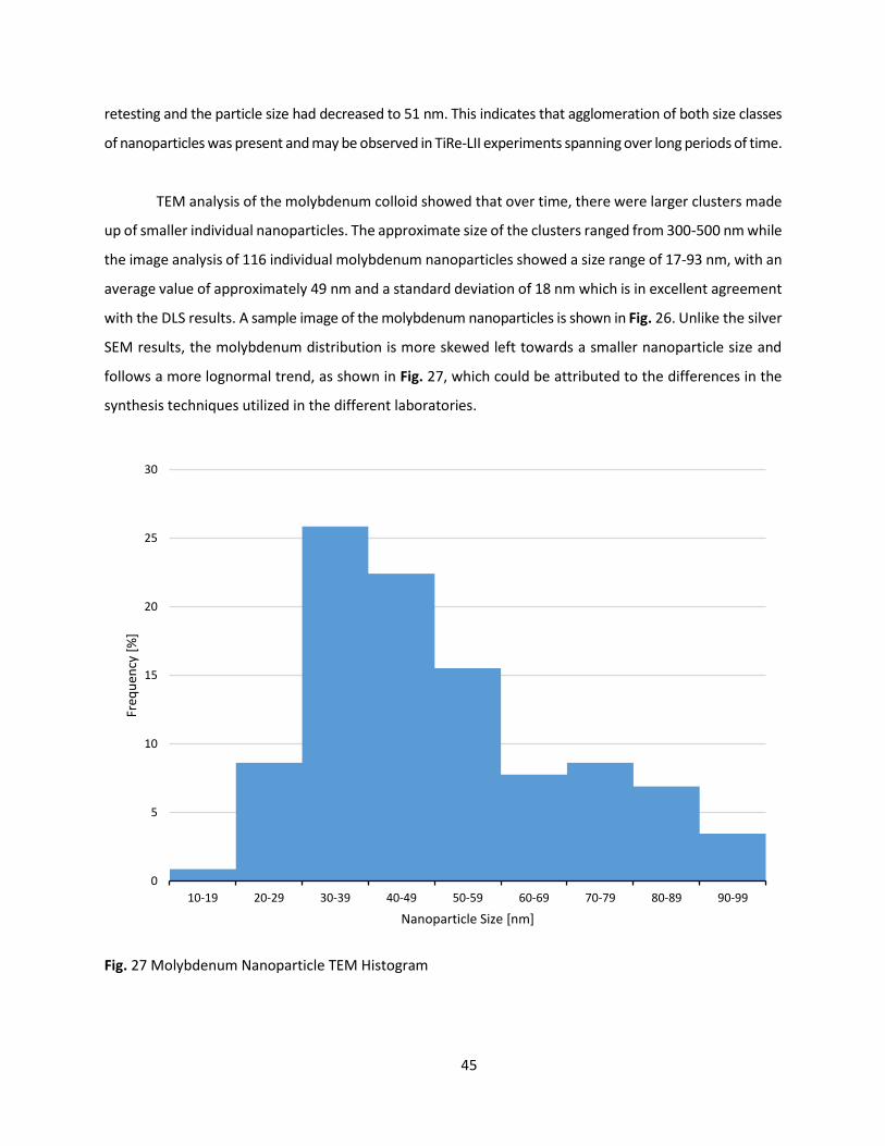
45
retesting and the particle size had decreased to 51 nm. This indicates that agglomeration of both size classes
of nanoparticles was present and may be observed in TiRe-LII experiments spanning over long periods of time.
TEM analysis of the molybdenum colloid showed that over time, there were larger clusters made
up of smaller individual nanoparticles. The approximate size of the clusters ranged from 300-500 nm while
the image analysis of 116 individual molybdenum nanoparticles showed a size range of 17-93 nm, with an
average value of approximately 49 nm and a standard deviation of 18 nm which is in excellent agreement
with the DLS results. A sample image of the molybdenum nanoparticles is shown in Fig. 26. Unlike the silver
SEM results, the molybdenum distribution is more skewed left towards a smaller nanoparticle size and
follows a more lognormal trend, as shown in Fig. 27, which could be attributed to the differences in the
synthesis techniques utilized in the different laboratories.
Fig. 27 Molybdenum Nanoparticle TEM Histogram
0
5
10
15
20
25
30
10-19 20-29 30-39 40-49 50-59 60-69 70-79 80-89 90-99
Freq
uen
cy [
%]
Nanoparticle Size [nm]

46
4.2 TiRe-LII Measurement Procedure
The following paragraphs describe the specific steps taken for each TiRe-LII measurement.
4.2.1 Preparation and Inspection
Before starting a TiRe-LII experiment, all of the gas tubing, and atomizer need to be inspected and
cleaned of any form of contamination since trace contaminants could result in false results. The TiRe-LII
setup is not designed to differentiate different incandescence sources so for example, residual soot or
previous metallic nanoparticles trapped within the apparatus may give erroneous results while testing
aerosols. All of the gas joints should be also be inspected to ensure that there are no leaks which may
result in gases and nanoparticles escaping into the breathing environment, causing potential health
concerns. To prevent this from happening, the exhaust stream from the TiRe-LII sample chamber is vented
into a nearby laboratory fumehood. The sample chamber should also be inspected for contamination
since the glass windows which are attached to it have previously been coated with the residue of the
nanoparticles that were previously tested. When the experiment is over, pressurized shop air should be
used to remove any residual nanoparticles that may have attached to the walls of any of the TiRe-LII
apparatus and associated tubing.
4.2.2 Nanocolloid Synthesis and Setup
Upon the verification of the TiRe-LII and TSI atomizer system, the nanoparticles of interest are
prepared as a colloid, and the carrier gas of interest is then used with the pneumatic atomizer to produce the
dry aerosol. First, the colloid is loaded into a 1 L bottle with a specialized cap which allows Swagelok
connections to the atomizer block. The carrier gas of interest is also connected to the atomizer block, and the
gas inlet pressure is maintained at 200 kPa using a gas cylinder regulator.
4.2.3 Activate TiRe-LII Apparatus
The TiRe-LII is then turned on, starting with the laser power source and then the PMT detector
module. After the instrument starts up the flashlamp Q-switch delay is checked using a remote keypad
attached to the laser module, and then the associated computer software is started, Artium integrated
management software (AIMS), and the appropriate experimental conditions are set, including the amount of
laser pulses per experiment and the measurement recording time. Prior to taking recording the measured
incandescence, trial runs are performed to ensure that the measured signals are not oversaturating the PMTs,
47
or to determine if the signal strength is too low, both of which are remedied by adjusting the PMT
amplification gain. When the trial measurements are within the operational limits, the signals are recorded
and then exported into Excel CSV files which contain the time-resolved incandesce signals at both detector
wavelengths. These measurements are repeated for the different aerosol mixtures as well as the fluence
study. Finally, throughout the TiRe-LII experiments, repeat measurements of the argon based aerosols are
made and then used to determine if the TiRe-LII derived nanoparticle size or TAC changes over time to infer
whether there is any type of measurement drift being caused by the nanoparticle chemistry changing,
including agglomeration and oxidation.
4.2.3 Shut Down and Cleanup
Upon completion of the TiRe-LII experiment, the instrument is shut down by first cutting off the
supply of the carrier gas of interest to the atomizer block, then the PMT detector module and laser power
source are turned off. Pressurized shop air is connected to the atomizer, and then the sample chamber to
remove any residual nanoparticles which may be trapped within the system. The remaining nanocolloid is
collected and disposed of in accordance to the laboratory disposal guidelines.
4.3 Laboratory Safety
All laboratory work in this study was conducted according to the policies outlined by the
University of Waterloo, in compliance with the workplace hazardous materials information system
regulations (WHMIS). This includes, reviewing the MSDS prior to working with any chemicals, using the
appropriate personal protective equipment (PPE) including lab coats and nitrile gloves, and the collection
and disposal of any hazardous waste. The TiRe-LII instrument utilizes a contained class 4 laser which may
cause permanent damage to the eyes, and burn skin if the appropriate precautions are not taken.
Exposure to the laser can occur only during the instrument’s calibration and maintenance since the laser
beam is kept within a sealed enclosure at all other times. To avoid potential injury when the laser
enclosure is removed, the appropriate laser glasses must be used as well as keeping the laser beam path
unobstructed when the laser is in operation.

48
Chapter 5 Results
Upon completion of a TiRe-LII experiment, the incandescence for both the nanoparticle heating
and cooling stages are recorded and then processed separately to determine the validity and application
of both the spectroscopic and heat transfer model proposed. The incandescence values are converted to
effective temperatures using two-colour pyrometry and the peak temperatures to serve as a first check
on whether the selected experimental or Drude theory derived E(m) values result in the temperatures
being physically realistic and how do these temperatures change when compared to the previous
assumption that E(m) only weakly changes as function of wavelength and can be treated as unity. The
nanoparticle cooling temperatures are used in the statistical model to recover the nanoparticle size and
TAC, when applicable. Finally the results of the nanoparticle size and TAC recovery using heat transfer
model with the selected physical parameters for the different iron, silver and molybdenum aerosol
mixtures are presented.
5.1 Fluence and Spectroscopic Results
The first component of TiRe-LII analysis is determining if there is any change in the observed peak
temperature when the laser fluence changes. In previous TiRe-LII studies conducted on soot [75], it was
expected that the observed peak TiRe-LII signal or its equivalent effective temperature to increase with
an increase of fluence until a plateau value is reached. This roughly corresponds to the sublimation
temperature, and indicates the point where additional laser energy is offset by increased heat losses
through phase change. By doing this analysis first, information could be gained to determine which heat
transfer modes will be dominant for the material being used.
The spectroscopic properties could also be validated by performing an energy balance during the
heat up stage of the TiRe-LII experiment. Following Eremin et al. [76] the complex index of refraction of
the nanoparticles at the excitation laser frequency can be inferred from the peak pyrometrically-defined
temperature found using E(m)r by performing an energy balance between the start of the laser pulse,
when the nanoparticles are at Tg, and the pyrometrically-defined peak nanoparticle temperature, Tp,max,
,max
3
6
p
in g abs cond evappqd
H HT qqT q
(22)

49
where H(Tg) and H(Tp,max) is the enthalpy of the material at Tg and Tp,max. Although Tp,max is due to a
balance between qabs, qevap, qcond, and the change in enthalpy of the nanoparticles, Eq. (20) can be
simplified by neglecting evaporation and conduction heat transfer before the peak nanoparticle
temperature is reached, in which case,
2 2 3
, 0 , 0 04laser laser laser laser
p p
abs abs
laser
abs
d dq C F Q F E F
m m (23)
where F0 is the laser fluence in units of J/cm2. Substituting Eq. (21) into Eq. (20) gives an expression for
E(mlaser),
,max
06laser
laser g p gT H T TH
FE
m (24)
where Eq. (22) could be used to approximate a lower bound estimate for E(mlaser). The following sections,
5.1.1-5.1.3, discuss the specific results for the iron, silver, and molybdenum experiments.
The peak temperatures of the iron nanoparticles were calculated using E(m)r = 0.539 taken from
Krishnan et al. [45]. The peak temperature was plotted against the laser fluence and is shown in Fig. 28
for the Ar, N2, and N2O aerosol mixtures, where the error bars correspond to one standard deviation from
the average peak temperature. At the time of testing CO2 gas was not available and was replaced with
another linear triatomic gas, N2O; from the remainder of the fluence analysis in this work and consistent
with Sipkens et al. [37], the peak temperatures calculated for each nanomaterial are independent of the
aerosol mixture being tested and which is in contrast to Eremin et al. [77] who observed that the peak
temperatures depended on the pressure and gas used in the aerosol mixture. A general trend observed
is that at the lower fluences, the measured incandescence have a very poor signal to noise ratio and the
standard deviation of the peak temperatures is significantly larger than the higher fluence measurements.
With the exception of the lowest fluence data point, all three aerosol mixtures showing an increasing peak
temperature as the fluence increases, from approximately 2750 K to 2850 K, well below the boiling point
of iron, 3134 K [58] and indicates that cooling occurs in a mixed conduction and evaporation dominant
regime. This result suggests that the energized nanoparticles is approaching the sublimation temperature
but due to the limitations with the selected TiRe-LII’s maximum fluence, further studies will be required
at higher fluences.

50
To get a lower bound estimate on E(mlaser), Eq. (22) was solved by setting the maximum
temperature equal to the boiling point, resulting in BP gH HT T
= 2026 kJ/kg taken from Desai
[56], and using F0 = 0.188 J/cm2 results in E(mlaser) = 0.479 which is significantly larger than the 0.065
value extrapolated from Krishnan et al. [45]. Sipkens et al. [37] reinterpreted from the data from Kock et
al. [18], and calculated E(mlaser) = 0.39 which is consistent with the value calculated in this study. To
provide a comparison of these results to the literature, the MLE recovered iron nanoparticle size, shown
in the next section, was used to calculate the size parameter and the E(mlaser) is plotted against the results
from Kock et al. [18], Eremin et al. [76], and the expected results from Mie theory, shown in Fig. 29. It can
be seen that all of the experimentally determined E(mlaser) values are larger than the Mie theory
calculated values, a result that requires further experiments to determine the root cause of this deviation.
Fig. 28 Peak temperature vs fluence for iron nanoparticles
2400
2500
2600
2700
2800
2900
3000
3100
0.1200 0.1400 0.1600 0.1800 0.2000 0.2200 0.2400 0.2600 0.2800
Pea
k Te
mp
erat
ure
[K
]
Fluence [J/cm2]
Ar
N2
N2O

51
Fig. 29 Comparison of the E(mlaser) from this study to the literature and Mie theory for iron
The peak temperatures of the silver nanoparticles were calculated using E(m)r = 0.366 derived
from Drude theory using the data from Krishnan et al. [45] and Miller [43]. The peak temperature was
plotted against the laser fluence and is shown in Fig. 30 for the Ar, N2, and CO2 aerosol mixtures, where
the error bars correspond to one standard deviation from the average peak temperature. All three aerosol
mixtures exhibit a maximum peak temperature of approximately 2800 K, well above silver’s boiling point
of 2466 K [59] and indicates that cooling occurs in an evaporation dominant regime. This result suggests
that they’re may be some superheating mechanism which is not being considered in the proposed models
but further investigation is required. Also, the peak temperatures are generally consistent regardless of
the fluence, unlike iron and molybdenum which show a general increase of peak temperature as the
fluence increases, but this could be attributed to the temperatures already exceeding the boiling point of
the silver nanoparticles.
0
0.1
0.2
0.3
0.4
0.5
0.6
0.001 0.01 0.1 1
E(m
Lase
r)
x = dp/
Eremin
Kock
Mie theory
Present Study

52
To get a lower bound estimate on E(mlaser), Eq. (22) was solved by setting the maximum
temperature equal to the boiling point, resulting in BP gH HT T
= 643 kJ/kg extrapolated from
Cagran et al. [57], and using F0 = 0.206 J/cm2 leads to E(mlaser) = 0.185 which is significantly larger than
the 0.017 and 0.014 values reported by Krishnan et al. [45], and Miller [43], respectively.
Fig. 30 Peak temperature vs fluence for silver nanoparticles
The peak temperatures of the molybdenum nanoparticles were calculated using E(m)r = 0.642
derived from the experimental data from Barnes at 2000 K [51]. The peak temperature was plotted against
the laser fluence and is shown in Fig. 31 for the Ar, N2, and CO2 aerosol mixtures, where the error bars
correspond to one standard deviation from the average peak temperature. Unlike the iron and silver
nanoparticles, the aerosol mixtures exhibit an increase of the calculated peak temperature as the laser
fluence increases, starting from approximately 2830 K at 0.206 J/cm2 and increasing to 2930 at 0.263
J/cm2, slightly above molybdenum’s melting point of 2896 K [50]. Due to the limitations of the TiRe-LII
instrument not being able to exceed fluences of 0.263 J/cm2, it is difficult to draw conclusions on whether
2000
2200
2400
2600
2800
3000
3200
3400
3600
0.2200 0.2250 0.2300 0.2350 0.2400 0.2450 0.2500 0.2550 0.2600 0.2650
Pea
k Te
mp
erat
ure
[K
]
Fluence [J/cm2]
Ar
N2
CO2

53
the system is approaching a steady state peak temperature as expected in soot from this experiment [75].
Another study from Eremin and Gurenstov [78] showed a possible steady-state peak temperature of
approximately 3900 K at fluences higher than 0.3 J/cm2 which is still significantly lower than the boiling
temperature of bulk molybdenum, 4913 K [60], and may require further investigation, possibly with
different particle sizes. To get a lower bound estimate on E(mlaser), Eq. (22) was solved by setting the
maximum temperature equal to the boiling point, resulting in BP gH HT T
= 10280 kJ/kg taken
from Desai [62] and using F0 = 0.206 J/cm2 in E(mlaser) = 0.038 which is consistent with the value
interpolated from Barnes [51] which is 0.065.
Fig. 31 Peak temperature vs fluence for molybdenum nanoparticles
Overall, it was shown that the E(mlaser) for iron and silver were significantly higher when
calculated using Eq. (22) using the data from the TiRe-LII experiments, when compared to the
approximated values from the data available from the literature while molybdenum is the only value that
is consistent between the TiRe-LII derived value and the value based on the literature value. Both iron and
2700
2750
2800
2850
2900
2950
3000
0.2000 0.2100 0.2200 0.2300 0.2400 0.2500 0.2600
Pea
k Te
mp
erat
ure
[K
]
Fluence [J/cm2]
Ar
N2
CO2

54
molybdenum showed an increase of the calculated peak temperatures as the laser fluence increased,
which was approaching their boiling and melting temperatures respectively, while silver showed a
consistent peak temperature well above its boiling point. From this, it is difficult to draw conclusions from
this analysis since the temperatures calculated are very sensitive to changes in the E(m) values used to
interpret the data. For example, the peak temperatures for silver is plotted again in Fig. 32 but calculated
for both E(m)r = 0.366 and E(m)r = 1, with the error bars omitted for clarity. It can be seen that the peak
temperatures calculated with E(m)r = 1 are approximately 3600-3800 K which is significantly higher than
the values calculated with E(m)r = 0.366, which is approximately 2700-2900 K. This result is consistent for
the other aerosol mixtures in this study and provides evidence for using accurate experimentally
determined E(m) values for molten metals. Since there is currently a lot of uncertainty in the optical
properties for these materials, there needs to be further research into obtaining more reliable
experimental values to minimize the error associated with using a specific E(m)r value.
Fig. 32 Peak temperature vs fluence for silver nanoparticles for E(m)r = 0.366 and E(m)r = 1
2400
2600
2800
3000
3200
3400
3600
3800
0.2200 0.2250 0.2300 0.2350 0.2400 0.2450 0.2500 0.2550 0.2600 0.2650
Pea
k Te
mp
erat
ure
[K
]
Fluence [J/cm2]
Ar
N2
CO2
Ar (Em=1)
N2 (Em=1)
CO2 (Em=1)

55
5.2 TiRe-LII Nanoparticle Size and TAC Analysis
The nanoparticle size and the TAC for each of the aerosol mixtures were attempted to be
recovered using the statistical framework previously outlined in Section 2.3. Using the peak temperature
values from section 5.1, the iron data was interpreted using a combined evaporation and conduction
model (x = [dp, TAC]T), silver with an evaporation only model (x = [dp]T), and conduction only model for
molybdenum. As previously stated, for molybdenum, the nanoparticle size to TAC ratio can only be
determined through the statistical framework, and will usually get trapped within a local minimum, so to
get useful information out of this process, the molybdenum nanoparticle size was set to the TEM
determined value of 49 nm and the TAC was recovered x = []. All three materials were expected to follow
a lognormal nanoparticle size distribution and the value of σg was selected to be 1.5 as per previous
studies [37].
5.2.1 Nanoparticle size and TAC recovery
The results for the iron nanoparticle TiRe-LII analysis are summarized in Table 3 using E(m)r =
0.539 taken from Krishnan et al. [45], and the uncertainties correspond to one standard deviation from
the measurement. From the previous sections and from previous studies [18, 37], it is expected that the
iron nanoparticle cooling occurs in the same temperature range which has sufficient heat transfer from
both conduction and evaporation, which allows for the simultaneous and as expected the model was able
to recover an optimal pair of the nanoparticle size and TAC which best fits the model to the data. The
recovered nanoparticle sizes are significantly smaller than the DLS calculated value of 41.9 nm, which
signifies that even though the model gives an excellent fit to the experimental values, there may be an
underlying deficiency in some of the material properties which is leading to this discrepancy, most of likely
being the E(m)r value. To attempt to improve upon the model fit, the E(m)r was adjusted until it was found
that E(m)r = 0.909 provided an improved fit of the modelled temperature to the experimental
temperatures, but is well above the experimental E(m)r value. The modeled and experimental
temperatures are shown in Fig. 33 for the E(m)r = 0.909 fit, and the contour plot used to determine the
uncertainty intervals is shown in Fig. 34 along with the MLE. As expected the signal to noise ratio decreases
as the measurement time increases, resulting in a poorer model fit to the data, notably at times exceeding
500 ns as shown in Fig. 33.

56
Table 3 Iron nanoparticle TiRe-LII size and TAC analysis
Gas x E(m)r = 0.539 E(m)r = 0.909
MLE Uncertainty MLE Uncertainty
Ar dp [nm] 11.0 0.07 32.7 1.9
TAC 0.091 0.002 0.24 0.03
N2 dp [nm] 10.3 0.1 29.9 1.0
TAC 0.028 0.0006 0.06 0.01
CO2 dp [nm] 10.4 0.06 29.0 1.4
TAC 0.051 0.0006 0.11 0.01
TEM dp [nm] 50-500 -
- DLS
dp [nm], 20 min 41.9 3.3
dp [nm], 40 min 151.9 14.9
Fig. 33 Plot of the experimental and modeled temperatures for the Fe-Ar aerosol

57
Fig. 34 Contour plot of the likelihood for the Fe-Ar aerosol
Throughout the experiment, there were visible changes in the colour of the iron nanocolloid,
which is attributed to the oxidation of the iron nanoparticles to iron oxide. This colour change is shown in
Fig. 35, at the synthesis completion where the mixture is homogenously black, at one hour where orange
a) b) c)
Fig. 35 Iron nanoparticle colloid colour at: a) synthesis completion; b) one hour; c) six hours

58
residue can be seen, and at approximately six hours where there is a significant amount of orange residue.
This was only observed for the iron nanoparticles as there was no apparent visual indicators for the silver
and molybdenum colloids; this should be further investigated in future experiments to determine if this
is truly the case. TiRe-LII measurements on the Fe-Ar mixture was repeated at 4 intervals over the duration
of the TiRe-LII experiment to determine if there were any changes in the TAC over time, and the results
are shown in Fig. 36. As shown, there is a gradual increase of the TAC over time, and for the second set of
measurements, there is a very large spread of TAC values calculated, with no experimental deviation from
the other sets of measurements.
Fig. 36 Time evolution of the TAC for a Fe-Ar mixture during a TiRe-LII experiment
The silver nanoparticle TiRe-LII measurements were interpreted using E(m)r = 0.366 derived from
Drude theory using the data from Krishnan et al. [45] and Miller [43], summarized in Table 4 along with
the one standard deviation error margins. From the previous sections, it is expected that the heat transfer
mode occurs in the evaporation only regime, and attempts to incorporate the conduction model in the
0.00
0.05
0.10
0.15
0.20
0.25
0.0 0.5 1.0 1.5 2.0 2.5 3.0
TAC
Time [hour]

59
interpretation of the data lead to unphysical values of the TAC being calculated. This included the TAC
being on the order of 103 in an attempt to increase the conduction model values to a comparable level to
the evaporation model. Since this is a nonphysical value as the TAC is an efficiency value bound between
0 and 1, the conduction model was disabled during this analysis. The TiRe-LII values for Ar and N2 with
each other but CO2 was noticeably smaller than the other aerosol mixtures. Also, the Ar and N2 values are
consistent with the DLS results, 87 nm, but are larger than the SEM results, 65 nm, which is consistent
with the CO2 values.
One of the key issues with silver nanoparticles and the TiRe-LII experiments, which was also
reported in the literature by Fillipov et al. [16], was that silver has poor optical properties in the visible
and infrared spectrum, and the measured incandescence values were consistent with this by exhibiting
poor signal strength. The TiRe-LII PMTs were set at their maximum operating gains which inherently
increases the magnitude of the electrical noise observed in the incandescence signals and overall,
resulting in a poor signal to noise ratio, even when the amount of measurements was increased to 500
runs per silver aerosol mixture. Another significant cause of this discrepancy is due to the fact that the
TiRe-LII measurements from this study and from the literature on silver occur on a much shorter time
scale than iron and molybdenum, at approximately < 80 ns [16] compared to over 500 ns [37, 19, 20],
respectively. Due to the poor signal to noise ratio, the incandescence signals are rarely usable after 80 ns
resulting in much less data being used to regress with the heat transfer model, and is a significant
contribution of the model’s uncertainty. This is shown in Fig. 37 where the modeled temperatures
generally capture the experimental temperatures cooling trend but fail to replicate the specific features
of the experimental data, with the associated contour plot shown in Fig. 38. The conduction model and
the TAC was used to calculate the likelihood with the evaporation model, but was still shown to have a
minimal impact on the likelihood demonstrated by the near one dimensional dependence on the
candidate nanoparticle size.

60
Table 4 Silver nanoparticle TiRe-LII size analysis
Gas x MLE Uncertainty
Ar dp [nm] 82 7
N2 dp [nm] 89 10
CO2 dp [nm] 75 8
SEM dp [nm] 65 12
DLS dp [nm], 0 min 87 4.4
dp [nm], 15 min 118 5.9
Fig. 37 Plot of the experimental and modeled temperatures for the Ag-Ar aerosol
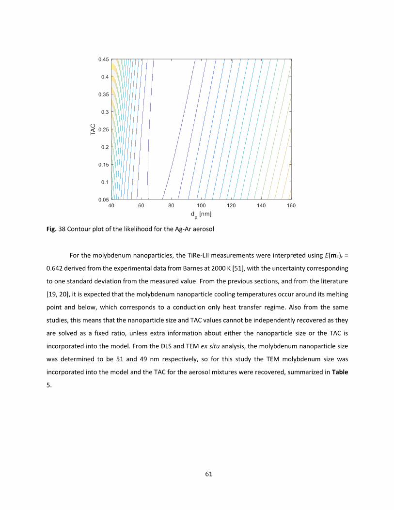
61
Fig. 38 Contour plot of the likelihood for the Ag-Ar aerosol
For the molybdenum nanoparticles, the TiRe-LII measurements were interpreted using E(m)r =
0.642 derived from the experimental data from Barnes at 2000 K [51], with the uncertainty corresponding
to one standard deviation from the measured value. From the previous sections, and from the literature
[19, 20], it is expected that the molybdenum nanoparticle cooling temperatures occur around its melting
point and below, which corresponds to a conduction only heat transfer regime. Also from the same
studies, this means that the nanoparticle size and TAC values cannot be independently recovered as they
are solved as a fixed ratio, unless extra information about either the nanoparticle size or the TAC is
incorporated into the model. From the DLS and TEM ex situ analysis, the molybdenum nanoparticle size
was determined to be 51 and 49 nm respectively, so for this study the TEM molybdenum size was
incorporated into the model and the TAC for the aerosol mixtures were recovered, summarized in Table
5.

62
Table 5 Molybdenum nanoparticle TiRe-LII TAC analysis using the TEM nanoparticle size
Gas x MLE Uncertainty
Ar TAC 0.24 0.002
N2 TAC 0.16 0.001
CO2 TAC 0.21 0.002
TEM dp [nm] 49 18
DLS dp [nm], no sonication 76 3.8
dp [nm], 15 min sonication
51 2.6
The modelled and experimental temperatures for the Mo-Ar mixture is shown in Fig. 39, where
the model only fit to the experimental temperatures outside of the anomalous cooling regime, which
occurs up to approximately 300 ns. A plot of the likelihood, calculated using the conduction model is
shown in Fig. 40, with the MLE nanoparticle size and TAC ratio labelled as the dashed line. As expected
the fixed ratio between the nanoparticle size and TAC can be seen from the almost linear arrangement of
the contour lines. This further supports that for conduction dominant TiRe-LII analysis, an ex situ method
of determining either the nanoparticle size or TAC is required to recover the other, or if there is prior
knowledge or approximate value of the expected TAC of the material being tested, the nanoparticle size
can be recovered, as the former was the case in this study.

63
Fig. 39 Plot of the experimental and modeled temperatures for the Mo-Ar aerosol
Fig. 40 Contour plot of the likelihood for the Mo-Ar aerosol

64
5.2.2 Perturbation Analysis
The recovered MLE values are contaminated with both the experimental noise as well as the
associated uncertainties of the material properties used in both the spectroscopic and heat transfer
models. Unfortunately, many of the error bounds for these parameters are not reported alongside their
associated literature values, so some of the key parameters which impact the models are identified and
perturbed to determine their impact on the recovered MLE values. These parameters and the
perturbation factor used, as a percent, are listed in Table 6.
Table 6 Sensitivity analysis overview of parameters and perturbation factors
Parameter Perturbation Factor [%]
Tg 0.5
5
cp 5
Hv 5a
Peak Temperature, Tp0 0.2
E(m)r 5
a Molybdenum does not use a conduction model so the effects of perturbing Hv are omitted
The perturbation factor is used to recalculate the MLE values for both the positive and negative
scaling of parameter of interest, and taking the average of these two values results in the parameter
induced error (PIE). The results of this analysis are shown in Fig. 41, Fig. 42, and Fig. 43 for the iron
nanoparticle size and TAC, silver nanoparticle size, and molybdenum TAC respectively. For the iron
nanoparticles this analysis was split between the nanoparticle size and TAC MLE values to see how the
parameters influence the recovered components individually. For the iron nanoparticle size, perturbing
E(m)r gave the largest deviation of approximately 46-48% , the carrier gas temperature showed almost
no influence on the nanoparticle size at <2%, and the remainder of the parameters showed a moderate
deviation from the nanoparticle size of approximately 10-20%.

65
For the silver nanoparticles, perturbing E(m)r and Hv gave the largest deviation of approximately
35-38% from the recovered nanoparticle size, the carrier gas had no observable effect with <1%, while
the peak initial temperature and the specific heat capacity showed a moderate contribution of
approximately 20%. Finally for the molybdenum nanoparticles, perturbing and cp gave the largest
deviation of approximately 21% from the recovered TAC value, while the remaining parameters deviated
approximately 10-15%. Overall, it can be seen that perturbing E(m)r results in the most significant
deviation from the recovered MLE values, although the contributions from the other parameters cannot
be neglected. It is reasonable to approximate the carrier gas temperature as the room temperature, but
the other parameters cannot be measured in real time, and accurate values with their error bounds need
Fig. 41 Perturbation analysis results for the nanoparticle size (left) and TAC (right) for iron
-20% 0% 20% 40% 60%
cp
DHv
Tg
Emr
Tp0
Parameter Induced Error
Per
turb
ed P
aram
eter
Fe-Ar Fe-N2 Fe-CO2
Tp0
E(m)r
Tg
Hv
cp
-20% 0% 20% 40% 60%
cp
DHv
Tg
Emr
Tp0
Parameter Induced Error
Per
turb
ed P
aram
eter
Fe-Ar Fe-N2 Fe-CO2
Tp0
E(m)r
Tg
Hv
cp

66
to be determined before interpreting the TiRe-LII data. Although it is not within the scope of this and
ongoing TiRe-LII studies, future work must include the accurate determination of the molten or high
temperature optical properties and temperature dependent physical properties of the materials of
interest.
Fig. 42 (Left) Perturbation analysis results for the nanoparticle size for silver Fig. 43 (Right) Perturbation analysis results for the TAC for molybdenum
-40% -20% 0% 20% 40% 60%
cp
DHv
Tg
Emr
Tp0
Parameter Induced Error
Per
turb
ed P
aram
eter
Ag-Ar Ag-N2 Ag-CO2
Tp0
E(m)r
Tg
Hv
cp
-30% -10% 10% 30%
r
cp
Tg
Emr
Tp0
Parameter Induced Error
Per
turb
ed P
aram
eter
Mo-Ar Mo-N2 Mo-CO2
Tp0
E(m)r
Tg
cp
67
Chapter 6 Conclusions and Future Work
This study was motivated by the need of developing a diagnostic which could provide real time
aerosolized nanoparticle size measurements in a safe environment. TiRe-LII is a soot diagnostic which has
been developed to conduct these nanoparticle size measurements. Previous TiRe-LII studies on synthetic
zero-valent metal nanoparticles had disadvantages including: using deficient heat transfer models, not
using the appropriate temperature dependent properties, or not being able to implement controls on the
synthesis of the nanoparticles which make comparing results between studies difficult. In this work, each
of the previous issues were addressed and the nanoparticle size and thermal accommodation coefficient
were recovered for iron, silver, and molybdenum nanoparticles, when applicable.
The heat transfer model and spectroscopic models, including the temperature dependent
material and optical properties required to interpret TiRe-LII measurements were presented and used to
simulate the heat transfer regimes for iron, silver, and molybdenum nanoparticles. It was shown that iron
has a mixture of both evaporation and conduction heat transfer modes, silver is dominated by
evaporation, and molybdenum is dominated by conduction. Next, the TiRe-LII instrument calibration and
setup was presented, including the laser alignment and energy measurements, as well as a brief discussion
on the atomizer setup and the ex situ characterization that was used to compare to the TiRe-LII
measurements. The nanoparticles were prepared as colloids instead of using previous gas based methods,
such as hot wall reactors or excimer lasers, which provided removed the previous effect that the carrier
gas had on the nanoparticle synthesis. The preparation steps for these colloids as well as their ex situ
characterization results were then presented, along with the TiRe-LII measurement procedure.
From the fluence and spectroscopic analysis, none of the calculated E(m) values for the TiRe-LII
instrument’s laser were consistent with the values approximated from the literature. Both iron and
molybdenum peak temperatures showed the expected trend of an increasing peak temperature as the
laser fluence increases while the silver nanoparticles peak temperatures were consistent for all fluences
tested, as well as, the peak temperature was significantly higher than the boiling point of silver, suggesting
a potential superheating effect that is not being accurately represented by the current models.
From the work done in this study, it was shown that the currently proposed heat transfer model
is suitable for the recovery of the nanoparticle size and TAC for iron nanoparticles, the nanoparticle size
for silver, and the nanoparticle size to TAC ratio for molybdenum. The TAC can be recovered for the

68
molybdenum nanoparticles if an ex situ derived nanoparticle size is previously determined and then used
as a known model parameter. With the associated error bounds provided, it was shown that the TiRe-LII
measured nanoparticle sizes were consistent with the ex situ nanoparticle sizes determined through
electron microscopy and dynamic light scattering. This strengthens the case that TiRe-LII could be adapted
to characterize synthetic aerosolized metal nanoparticles, provided that the spectroscopic and heat
transfer models are well developed, as well as credible optical and physical properties of the tested
nanomaterials are used.
From these results, the future studies should focus on the improvement of the error associated
with the optical and physical properties of the nanoparticles used. From the perturbation analysis, almost
all of the properties used in the model contributed a significant deviation from the TiRe-LII determined
when a small perturbation factor was applied. Ongoing experiments are attempting to address these
issues by using additional nanomaterials which may have better error bounds on their optical and physical
properties, including silicon, copper, and nickel. Also, further time evolution studies and reanalysis of the
previous work should be conducted to determine if there is any change in the nanoparticle morphology
during an experiment which have been shown to present in the TiRe-LII size measurements for iron
nanoparticles.

69
References
[1] T. M. Tolaymat, A. M. El Badaway, A. Genaidy, K. G. Scheckel, T. P. Luxton and M. Suidan, "Review -
An evidence based envionmental perspective of manufactured silver nanoparticle in sytheses and
applications: A systematic review and critical appraisal of peer-reviewed scientific papers," Sci. Total
Environ., vol. 408, no. 5, pp. 999-1006, 2010.
[2] D. C. Huber, "Synthesis, Properties, and Applicatins of Iron Nanoparticles," Small, vol. 1, no. 5, pp.
482-501, 2005.
[3] J. Park, E. Lee, N. M. Hwang, M. Kang, S. C. Kim, Y. Hwang, J. G. Park, H. J. Noh, J. Y. Kim, J. H. Park
and T. Hyeon, "One-Nanometer-Level Size-Controlled Synthesis of Monodisperse Magnetic Iron
Oxide Nanoparticles and their Structural and Magnetic Characterization," Angew. Chem. Int. Edit.,
vol. 44, no. 19, pp. 2872-2877, 2005.
[4] G. Chen, I. Roy, C. Yang and P. N. Prasad, "Nanochemistry and Nanomedicine for Nanoparticle-based
Diagnostics and Therapy," Chem. Rev., vol. 116, no. 5, pp. 2826-2885, 2016.
[5] D. Wang, T. Xie and Y. Li, "Nanocrystals: Solution-based synthesis and applications as nanocatalysts,"
Nano Research, vol. 2, no. 1, pp. 30-46, 2009.
[6] H. H. Lara, N. V. Ayala-Nunez, L. C. I. Turrent and C. R. Padilla, "Bactericidal effect of silver
nanoparticles against multidrug-resistant bacteria," World J. Microb. Biot., vol. 26, no. 4, pp. 615-
621, 2010.
[7] M. Stefaniuk, P. Oleszczuk and Y. S. Ok, "Review on nano zerovalent iron (nZVI): From synthesis to
environmental applications," Chem. Eng. J., vol. 287, pp. 618-632, 2016.
[8] T. Phenrat, T. C. Long, G. V. Lowry and B. Veronesi, "Partial Oxidation (“Aging”) and Surface
Modification Decrease the Toxicity of Nanosized Zerovalent Iron," Environ. Sci. Technol., vol. 43, no.
1, pp. 195-200, 2009.
[9] C. R. Keenan, R. Goth-Goldstein, D. Lucas and D. L. Sedlak, "Oxidative Stress Induced by Zero-Valent
Iron Nanoparticles and Fe(II) in Human Bronchial Epithelial Cells," Environ. Sci. Technol., vol. 43, no.
12, pp. 4555-4560, 2009.
[10] S. Gaillet and J. M. Rouanet, "Silver nanoparticles: Their potential toxic effects after oral exposure
and underlying mechanisms – A review," Food Chem. Toxicol., vol. 77, pp. 58-63, 2015.
70
[11] K. Sheehy, A. Casey, A. Murphy and G. Chambers, "Antimicrobial properties of nano-silver: A
cautionary approach to ionic interference," J. Colloid Interf. Sci., vol. 443, pp. 56-64, 2015.
[12] L. Braydich-Stolle, S. Hussain and M. C. Hofmann, "In Vitro Cytotoxicity of Nanoparticles in
Mammalian Germline Stem Cells," Toxicol. Sci., vol. 88, no. 2, pp. 416-419, 2005.
[13] L. A. Melton, "Soot Diagnostics Based on Laser Heating," Appl. Opt., vol. 23, no. 13, pp. 2201-2208,
1984.
[14] S. Schraml, S. Will and A. Leipertz, "Simultaneous Measurement of Soot Mass Concentration and
Primary Particle Size in the Exhaust of a DI Diesel Engine by Time-Resolved Laser-Induced
Incandescence (TIRE-LII)," SAE Paper, no. 01-0146, 1999.
[15] B. F. Kock, T. Eckhardt and P. Roth, "In-Cylinder Sizing of Diesel Particles by Time-Resolved Laser-
Induced Incandescence (TR-LII)," P. Combust. Inst., vol. 29, no. 2, pp. 2775-2782, 2002.
[16] A. V. Fillipov, M. W. Markus and P. Roth, "In-Situ Characterization of Ultrafine Particles by Laser-
Induced Incandescence: Sizing and Particle Structure Determination," J. Aerosol Sci., vol. 30, no. 1,
pp. 71-87, 1999.
[17] R. Starke, B. Kock and P. Roth, "Nano-particle Sizing by laser-Induced Incandescence (LII) in a Shock
Wave Reactor," Shock Waves, vol. 12, no. 5, pp. 351-260, 2003.
[18] B. F. Kock, C. Cayan, J. O. H. R. Knipping and P. Roth, "Comparison of LII and TEM sizing during
synthesis of iron particle chains," P. Combust. Inst., vol. 30, pp. 1689-1697, 2005.
[19] Y. Murakami, T. Sugatani and Y. Nosaka, "Laser-Induced Incandescence Study on the Metal Aerosol
Particles as the Effect of the Surrounding Gas Medium," J. Phys. Chem. A, vol. 109, no. 40, pp. 8994-
9000, 2005.
[20] T. Sipkens, G. Joshi, K. J. Daun and Y. Murakami, "Sizing of Molybdenum Nanoparticles using Time-
Resolved Laser-Induced Incandescence," J. Heat Transf., vol. 135, no. 5, 2013.
[21] T. A. Sipkens, R. Mansmann, K. J. Daun, N. Petermann, J. T. Titantah, M. Karttunen, H. Wiggers, T.
Dreier and C. Schulz, "In Situ Particle Sizing of Silicon Nanoparticles by Time-Resolved Laser-Induced
Incandescence," Appl. Phys. B, vol. 116, no. 3, pp. 623-636, 2014.
[22] N. R. Singh, T. A. Sipkens, K. J. Daun, N. Bizmark and M. Ioannidis, "Aerosolized Iron Nanoparticle
Size Measurements Using Time Resolved Laser Induced Incandescence," in 2014 CI/CS Spring
Technical Meeting, Windsor, 2014.

71
[23] K. J. Daun, G. J. Smallwood and F. Liu, "Investigation of Thermal Accommodation Coefficients in
Time-Resolved Laser-Induced Incandescence," J. Heat Trans., vol. 130, no. 12, 2008.
[24] A. Boiarciuc, F. Foucher and C. Mounaim-Rousselle, "Soot Volume Fractions and Primary Particle Size
Estimate by Means of the Simultaneous Two-Color-Time-Resolved and 2D Laser-Induced
Incandescence," Appl. Phys. B, vol. 83, no. 3, pp. 413-421, 2006.
[25] J. Black and M. Johnson, "In-Situ Laser-Induced Incandescence of Soot in an Aero-Engine Exhaust:
Comparison with Certification Style Measurements," Aerosp. Sci. Technol., vol. 14, no. 5, pp. 329-
337, 2010.
[26] R. L. Vander Wal, T. M. Ticich and J. R. West, "Laser-Induced Incandescence Applied to Metal
Nanostructures," Appl. Opt., vol. 38, no. 27, pp. 5867-5879, 1999.
[27] F. Liu, K. J. Daun, D. R. Snelling and G. J. Smallwood, "Heat Conduction from a Spherical Nano-
Particle: Status of Modelling Heat Conduction in Laser-Induced Incandescence," Appl. Phys. B, vol.
83, no. 3, pp. 355-382, 2006.
[28] A. Eremin, E. Gurentsov and C. Schulz, "Influence of the Bath Gas on the Condensation of
Supersaturated Iron Atom Vapour at Room Temperature," J. Phys. D: Appl. Phys., vol. 41, no. 5, pp.
1-5, 2008.
[29] K. J. Daun, "Thermal Accommodation Coefficients Between Polyatomic Gas Molecules and Soot in
Laser-Induced Incandescence Experiments," Int. J. Heat Mass Transfer, vol. 52, no. 21, pp. 5081-
5089, 2009.
[30] K. J. Daun, J. T. Titantah and M. Karttunen, "Molecular Dynamics Simulation of Thermal
Accommodation Coefficients for Laser-Induced Incandescence Sizing of Nickel Particles," Appl. Phys.
B, vol. 107, no. 1, pp. 221-228, 2012.
[31] J. Reimann, H. Oltmann, S. Will, C. Bassano, E. L. Lösch and S. Günther, "Laser Sintering of Nickel
Aggregates Produced from Inert Gas Condensation," in Proceedings of the World Conference on
Particle Technology, Nuremberg, Germany, 2010.
[32] T. Lehre, R. Suntz and H. Bockhorn, "Time-Resolved Two-Color LII: Size Distributions of Nano-
Particles from Gas-to-Particle Synthesis," P. Combust. Inst., vol. 30, no. 2, pp. 2585-2593, 2005.
[33] F. Cignoli, C. Bellomunno, S. Maffi and G. Zizak, "Laser-Induced Incandescence of Titania
Nanoparticles Synthesized in a Flame," Appl. Phys. B, vol. 96, no. 4, pp. 593-599, 2009.

72
[34] S. Maffi, F. Cignoli, C. Bellomunno, S. De luliis and G. Zizak, "Spectral Effects in Laser Induced
Incandescence Application to Flame-made Titania Nanoparticles," Spectrochim. Acta B, vol. 63, no.
2, pp. 202-209, 2009.
[35] B. Tribalet, A. Faccinetto, T. Dreier and C. Schultz, "Evaluation of Particle Sizes of Iron-Oxide Nano-
Particles in a Low-Pressure Flame-Synthesis Reactor by Simultaneous Application of TiRe-LII and
PMS," in 5th Workshop on Laser-induced Incandescence, Le Touquet, France, 2012.
[36] I. S. Altman, D. Lee, J. Song and M. Choi, "Experimental Estimate of Energy Accommodation
Coefficient at High Temperatures," Phys. Rev. E, vol. 64, no. 5, 2001.
[37] T. A. Sipkens, N. R. Singh, K. J. Daun, N. Bizmark and M. Ioannidis, "Examination of the Thermal
Accommodation Coefficient Used in the Sizing of Iron Nanoparticles by Time-Resolved
Laser-Induced Incandescence," Appl. Phys. B, vol. In press., 2015.
[38] M. F. Modest, Radiative Heat Transfer, 3rd Ed., San Diego: Academic Press, 2013.
[39] D. R. Snelling, G. J. Smallwood, F. Liu, O. L. Gulder and W. D. Bachalo, "A Calibration-Independent
Laser-Induced Incandescence Technique for Soot Measurement by Detecting Absolute Light
Intensity," Appl. Opt., vol. 44, no. 31, pp. 6773-6785, 2005.
[40] T. C. Bond and R. W. Bergstrom, "Light Absorption by Carbonaceous Particles: An Investigative
Review," Aerosol Sci. Tech., vol. 40, pp. 27-67, 2006.
[41] J. A. Creighton and D. G. Eadon, "Ultraviolet-Visible Absorption Spectra of the Colloidal Metallic
Elements," J. Chem Soc. Faraday Trans., vol. 87, pp. 3881-3891, 1991.
[42] K. M. Watson, "Thermodynamics of the Liquid State," Ind. Eng. Chem., vol. 35, no. 4, pp. 398-406,
1943.
[43] J. C. Miller, "Optical Properties of Liquid Metals at High Temperatures," Phil. Mag., vol. 20, no. 168,
pp. 1115-1132, 1969.
[44] J. N. Hodgson, "Infra-red Measurements of the Optical Constants of Liquid Silver," Philos. Mag., vol.
5, pp. 272-277, 1960.
[45] S. Krishnan, G. P. Hansen, R. H. Hauge and J. L. Margrave, "Spectral Emissiviites and Optical
Properties of Electromagnetrically-Levitated Liquid Metals as Functions of Temperature and
Wavelength," High Temp. Sci., vol. 29, pp. 17-52, 1990.
[46] C. F. Bohren and D. R. Huffman, Absorption and Scattering of Light by Small Particles, New York:
John Wiley & Sons, 1983.

73
[47] M. Quinten, Optical Properties of Nanoparticle Systems: Mie and Beyond, New York: John Wiley and
Sons, 2011.
[48] H. Kobatake, H. Khosroabadi and H. Fukuyama, "Normal spectral emissivity measurement of liquid
iron and nickel using electromagnetic levitation in direct current magnetic field," Met. Trans. A, vol.
43A, pp. 2466-2472, 2012.
[49] T. E. Faber, Introduction to the Theory of Liquid Metals, Cambridge, UK: Cambridge University Press,
1972.
[50] P. F. Paradis, T. Ishikawa and Y. Nosaka, "Noncontact Measurements of Thermophysical Properties
of Molybdenum at High Temperatures," Int. J. Thermophys., vol. 23, no. 2, pp. 555-569, 2002.
[51] B. T. Barnes, "Optical Constants of Incandescent Refractory Metals," J. Opt. Soc. AM, vol. 56, pp.
1546-1550, 1966.
[52] D. W. Juenker, L. J. LeBlanc and C. R. Martin, "Optical properties of some transition metals," J. Opt.
Soc. AM, vol. 58, pp. 164-171, 1968.
[53] E. D. Palik, Handbook of Optical Constants of Solids, London: Elsevier, 2012.
[54] R. S. Hixson, M. A. Winkler and M. L. Hodgdon, "Sound Speed and Thermoyhysical Properties of
Liquid Iron and Nickel," Phys. Rev. B, vol. 42, no. 10, pp. 6485-6491, 1990.
[55] A. V. Grosse and A. D. Kirshenbaum, "The temperature range of liquid lead and silver and an estimate
of their critical constants," J. Inorg. Nucl. Chem., vol. 24, pp. 739-748, 1962.
[56] P. D. Desai, "Thermodynamic Properties of Iron and Silicon," J. Phys. Chem. Ref. Data, vol. 15, no. 3,
pp. 967-983, 1986.
[57] C. Cagran, W. Wilthan and G. Pottlacher, "Enthalpy, Heat of Fusion, and Specific Electrical Resistivity
of Pure Silver, Pure Copper, and the Binary Ag-28Cu Alloy," Thermochim. Acta, vol. 445, pp. 104-110,
2006.
[58] J. A. Dean, Lange's Handbook of Chemistry, 15th ed., McGraw-Hill, 1999.
[59] F. Mafune, J.-Y. Kohno, Y. Takeda and T. Kondow, "Formation of Stable Platinum Nanoparticles by
Laser Ablation in Water," J. Phys. Chem. B , vol. 107, pp. 4218-4223, 2003.
[60] CRC Handbook of Chemistry and Physics, 96th Edition, 2015-2016, Cleveland, Ohio: CRC Press, 2015.
[61] D. A. Young and B. J. Alder, "Critical Point of Metals from the van der Waals Model," Phys. Rev. A,
vol. 3, no. 1, pp. 364-371, 1971.

74
[62] P. D. Desai, "Thermodynamic Properties of Manganese and Molybdenum," J. Phys. Chem. Ref. Data,
vol. 16, no. 1, pp. 91-108, 1987.
[63] B. J. Keene, "Review of Data for the Surface Tension of Iron and its Binary Alloys," Int. Mater. Rev.,
vol. 33, no. 1, 1988.
[64] R. Novakovic, E. Ricci, D. Giuranno and A. Passerone, "Surface and transport properties of Ag-Cu
liquid Alloys," Surf. Sci., vol. 576, pp. 175-187, 2005.
[65] H. M. Lu and Q. Jiang, "Surface Tension and Its Temperature Coefficient for Liquid Metals," J. Phys.
Chem. B, vol. 109, no. 32, pp. 15463-15468, 2005.
[66] T. A. Sipkens, R. Mansmann, K. J. Daun, N. Petermann, J. T. Titantah, M. Karttunen, H. Wiggers, T.
Dreier and C. Schulz, "In Situ Nanoparticle Size Measurements of Gas-Borne Silicon Nanoparticles by
Time-Resolved Laser-Induced Incandescence," Appl. Phys. B, vol. 116, no. 3, pp. 623-636, 2013.
[67] P. C. Hiemenz and R. Rajagopalan, Principles of Colloid and Surface Chemistry Third Edition, Revised
and Expanded, Boca Raton: CRC Press, Taylor & Francis Group, 1997.
[68] Y. Leng, Materials Characterization Introduction to Microscopy and Spectroscopic Methods,
Singapore: John Wiley & Sons (Asia) Pte Ltd, 2008.
[69] Y. Liu, S. A. Majetich, R. D. Tilton, D. S. Scholl and L. and G. V., "TCE Dechlorination Rates, Pathways,
and Efficiency of Nanoscale Iron Particles with Different Properties," Environ. Sci. Tech., vol. 39, no.
5, pp. 1338-1345, 2005.
[70] F. He and D. Zhao, "Manipulating the Size and Dispersibility of Zerovalent Iron Nanoparticles by use
of Carboxymethyl Cellulose Stabilizers," Environ. Sci. Technol., vol. 41, no. 17, pp. 6216-6221, 2007.
[71] T. Phenrat, H. J. Kim, F. Fagerlund, T. Illangasekare, R. D. Tilton and G. V. Lowry, "Particle Size
Distribution, Concentration, and Magnetic Attraction Affect Transport of Polymer-Modified Fe0
Nanoparticles in Sand Columns," Environ. Sci. Technol., vol. 43, no. 15, pp. 5079-5085, 2009.
[72] P. C. Lee and D. Meisel, "Adsorption and surfance-enhanced Raman of dyes on silver and gold sols,"
J. Phys. Chem, vol. 86, no. 17, pp. 3391-3395, 1982.
[73] A. D. Rakić, A. B. Djurišić, J. M. Elazar and M. L. Majewski, "Optical properties of metallic films for
vertical-cavity optoelectronic devices," Appl. Opt., vol. 37, no. 22, pp. 5271-5283, 1998.
[74] M. A. Ordal, R. J. Bell, R. W. Alexander, L. L. Long and M. R. Querry, "Optical properties of fourteen
metals in the infrared and far infrared: Al, Co, Cu, Au, Fe, Pb, Mo, Ni, Pd, Pt, Ag, Ti, V, and W," Appl.
Opt., vol. 24, no. 24, pp. 4493-4499, 1985.
75
[75] S. De Iuliis, F. Migliorini, F. Cignoli and G. Zizak, "Peak soot temperature in laser-induced
incandescence measurements," Appl. Phys. B, vol. 2006, pp. 397-402, 2005.
[76] A. Eremin, E. Gurentsov, E. Popova and K. Priemchenko, "Size Dependence of Complex Refractive
Index Function of Growing Nanoparticles," Appl. Phys. B, vol. 104, no. 2, pp. 289-295, 2011.
[77] A. Eremin, E. Gurentsov, E. Mikheyeva and K. Priemchenko, "Experimental Study of Carbon and Iron
Nanoparticle Vaporisation Under Pulse Laser Heating," Appl. Phys. B, vol. 112, no. 3, pp. 421-432,
2013.
[78] A. V. Eremin and E. V. Grentsov, "Sizing of Mo Nanoparticles Synthesized by Kr-F Laser Pulse Photo-
Dissociation of Mo(CO)6," Appl. Phys. A, vol. 119, pp. 615-622, 2015.