Embed Size (px)
Citation preview

TIME SAVINGS IN PRODUCT DEVELOPMENT THROUGH CONTINUOUS SIMULATION
by
Andrew H Martin
BSME, University of Pittsburgh, 2003
BAMA, St. Vincent College, 2002
Submitted to the Graduate Faculty of
School of Engineering in partial fulfillment
of the requirements for the degree of
Master of Science Industrial Engineering
University of Pittsburgh
2005

UNIVERSITY OF PITTSBURGH
SCHOOL OF ENGINEERING
This thesis was presented
by
Andrew H Martin
It was defended on
April 14, 2005
and approved by
Dr. Bopaya Bidanda, Professor, Dept. of Industrial Engineering
Dr. Rabikar Chatterjee, Professor, Katz Graduate School of Business
Thesis Advisor: Dr. Michael R. Lovell, Associate Dean for Research, Associate Professor, Dept. of Industrial Engineering
ii

TIME SAVINGS IN PRODUCT DEVELOPMENT THROUGH CONTINUOUS SIMULATION
Andrew H Martin, MS
University of Pittsburgh, 2005
Today’s fast-paced economy and complex global market has made it difficult for
manufacturing companies to maintain their competitive edge. Products being developed
today must stand apart from others, and lead the market in the way they meet customer
needs. Tools to reduce product development time have been in use for decades, but
recently new tools have become available to make significant reductions in the product
development cycle. Specifically, simulation tools are becoming very useful for saving
time in the design-build-test phase of product development.
New simulation tools that compress the product development cycle change the
way design errors are found and refined. Traditional product development would create
a design, prototype that design, and test it for failures, then repeat the process until the
performance was acceptable. A newly developed process combines CAD, CAE, and
FEA simulation tools to create an interactive feedback loop in the front part of product
development to significantly reduce development time.
DesignXplorer VT (DX-VT) uses CAD, CAE, and FEA to form an easy to operate
virtual simulation tool that can be used by engineers and designers in multiple stages of
product development. From generating innovative designs, to shedding light on how
designs can be optimized for peak performance, DX-VT has tools to make product
development easier. Using DX-VT in the concept design stage and throughout the CAE
analysis and testing stage will give designers and engineers a complete breakdown of
what design parameters need changed.
iii

I have used DX-VT to create a benchmark test of how the software can be used
for product development. I have used real world virtual prototypes from Technip Inc. to
evaluate the realistic applications of this software. To capture this process a best
practices guide was created to be a general guide on how to efficiently use Workbench
Design Modeler, Simulation, and DesignXplorer for enhancing product development.
This guide was tailored to Technip Inc. and their most recent project, the Red Hawk.
The best practices guide demonstrates how to use the Ansys Workbench software to
simulate actual components from the Red Hawk oil rig. The guide shows all the steps
and features that were required to get this real life model to solve properly. The results
of this product development process will cut development time at Technip by 1000’s of
man hours, and help in their goal to cut design costs by $2 million per project.
iv

TABLE OF CONTENTS
LIST OF TABLES............................................................................................................ vii
LIST OF FIGURES ......................................................................................................... viii
ACKNOWLEDGEMENTS.............................................................................................. xii
1.0 INTRODUCTION ....................................................................................................... 1
1.1 CUTTING PRODUCT DEVELOPMENT TIME ........................................ 2
1.1.1 Better Engineering ............................................................................ 2
1.1.2 Better Manufacturing ........................................................................ 3
1.1.3 Better Marketing ............................................................................... 4
1.1.4 Better Managing................................................................................ 4
1.1.5 Future improvement to product development................................... 5
2.0 BACKGROUND ......................................................................................................... 6
2.1 TRADITIONAL PRODUCT DEVELOPMENT CYCLE............................ 6
2.2 TRADITIONAL PROTOTYPING PHASES............................................... 8
2.2.1 Manual .............................................................................................. 8
2.2.2 Virtual ............................................................................................... 8
2.2.3 Rapid ................................................................................................. 9
2.2.4 Advantages of Virtual Prototyping ................................................. 10
2.3 HISTORY OF FEA ..................................................................................... 11
2.4 TRADITIONAL VIRTUAL PROTOTYPING PROCESS ....................... 12
3.0 A NEW VIRTUAL PROTOTYPING PROCESS..................................................... 14
v
3.1 TOOLS ARE BECOMING COMMONLY USED .................................... 16
3.2 TOOLS GIVE MORE CREATIVITY TO DESIGNERS ......................... 16
3.3 TEST IDEAS EARLY, ELIMINATE INFERIOR DESIGNS................... 18
3.4 STILL A NEED FOR RAPID PROTOTYPING ....................................... 19
4.0 RESULTS OF THIS NEW VIRTUAL PROTOTYPING PROCESS ...................... 20
5.0 ANSYS DESIDNXPLORER VT TOOLS ................................................................ 22
6.0 IMPLEMENTING SIMULATION TOOLS ............................................................. 25
7.0 TECHNIP CASE ....................................................................................................... 26
8.0 SOLUTIONS FOR TECHNIP................................................................................... 29
9.0 CONCLUSION.......................................................................................................... 34
APPENDIX....................................................................................................................... 38
vi

LIST OF TABLES
Table 1: Rapid Prototyping History [5].................................................................. 9
vii

LIST OF FIGURES
Figure 1: Product development Cycle [4] ................................................................................ 6
Figure 2: Compressed product development cycle [6]........................................................ 15
Figure 3: Feedback Loop in Early Product Development [6] ............................................. 17
Figure 4: Red Hawk model ...................................................................................................... 27
Figure 5: Gantt Chart of Original Red Hawk Project ............................................................ 28
Figure 6: Bulk Head model in Autodesk Inventor.................................................................. 30
Figure 7: Mid-surfaced Faces ................................................................................................. 31
Figure 8: Gantt Chart of reduced production time ............................................................... 35
Figure 9: Reduced engineering and design time ................................................................. 36
Figure 10: Ansys Opening Screen ......................................................................................... 39
Figure 11: Import External Geometry .................................................................................... 39
Figure 12: Generate button ..................................................................................................... 40
Figure 13: Options Button........................................................................................................ 40
Figure 14: User Interface Options .......................................................................................... 41
Figure 15: Mid-Surface button ................................................................................................ 42
Figure 16: Mid-Surface Features............................................................................................ 42
Figure 17: Mid-surfaced Faces ............................................................................................... 43
Figure 18: Surface Extension Button ..................................................................................... 44
Figure 19: Surface Extension Features ................................................................................. 44
viii

Figure 20: Additional Surface Extension Features .............................................................. 44
Figure 21: Thin/Surface Button ............................................................................................... 45
Figure 22: Thin/Surface Features........................................................................................... 46
Figure 23: Joint Button ............................................................................................................. 47
Figure 24: Joint Features ......................................................................................................... 47
Figure 25: Select Parts from Geometry Tree........................................................................ 48
Figure 26: Form New Part Button........................................................................................... 48
Figure 27: Set Parameters ...................................................................................................... 49
Figure 28: Start New Simulation ............................................................................................. 50
Figure 29: Rename Contact Based on Geometry Button ................................................... 51
Figure 30: Deleting Duplicate Contact ................................................................................... 52
Figure 31: Setting Contact Pinball Size ................................................................................. 53
Figure 32: Inserting Contact Tool ........................................................................................... 53
Figure 33: Deleting Inactive Contact...................................................................................... 54
Figure 34: Setting Material Properties ................................................................................... 54
Figure 35: Preview Mesh Button ............................................................................................ 55
Figure 36: Insert Mesh Sizing ................................................................................................. 56
Figure 37: Mesh Sizing Details ............................................................................................... 56
Figure 38: Insert Mesh Refinement........................................................................................ 57
Figure 39: Insert Mapped Face Meshing .............................................................................. 58
Figure 40: Insert Structural Loads .......................................................................................... 59
Figure 41: Insert Supports ....................................................................................................... 59
Figure 42: Insert Solution Criteria........................................................................................... 60
ix

Figure 43: Insert Solution Criteria........................................................................................... 61
Figure 44: Set Input Parameters ............................................................................................ 62
Figure 45: Set Output Parameters ......................................................................................... 62
Figure 46: Solution Settings .................................................................................................... 63
Figure 47: Solve Button............................................................................................................ 64
Figure 48: View of Total Deformation Solution..................................................................... 65
Figure 49: View of Maximum Principle Stress Solution ...................................................... 65
Figure 50: Simulation Design Report ..................................................................................... 66
Figure 51: Solution Settings .................................................................................................... 67
Figure 52: Start New DesignXplorer VT Study..................................................................... 69
Figure 53: Select Input Parameters ....................................................................................... 69
Figure 54: Parameter Details .................................................................................................. 70
Figure 55: Solve in ANSYS Button......................................................................................... 71
Figure 56: Responses Button.................................................................................................. 72
Figure 57: Response to Input Parameters ............................................................................ 72
Figure 58: Sample Generation ................................................................................................ 73
Figure 59: Goals for Input Parameters .................................................................................. 74
Figure 60: Goals for Output Parameters ............................................................................... 74
Figure 61: Sample Generation Button ................................................................................... 75
Figure 62: Candidate Designs ................................................................................................ 75
Figure 63: Best Candidate Designs ....................................................................................... 76
Figure 64: Sensitivities ............................................................................................................. 77
Figure 65: Tradeoff Plot 3D ..................................................................................................... 78
x

Figure 66: DX Reports.............................................................................................................. 79
xi
ACKNOWLEDGEMENTS
I would like to thank Dr. Michael R. Lovell for his endless generosity he has
shown to me. He has given me ample amounts of his time, resources, facilities,
contacts, and even his advice, all in an effort to make graduate school more
manageable yet exciting for myself. I also thank Dr. Rabikar Chatterjee and Dr. Jayant
Rajgopal for creating a dual masters degree program that has run so smoothly for
myself and my fellow classmates. I want to thank Dr. Lovell and Dr. Chatterjee for
focusing my graduate program only to the topics I am interested in. It is rare to find
faculty so concerned with their student’s interests.
I need to thank Jim Maher and the staff of Technip Inc. for their cooperation,
hospitality in Houston, and priceless insight into their problems with product
development. A special thank you to Chandra Sekaran, Chris Boda, Aaron Benek,
Jean-Daniel Beley, and the staff of Ansys Inc who helped me for eighteen months to
learn, develop, and use Ansys software correctly.
I dedicate this project foremost to my family. They have supported me for twenty
years of education with love, admiration, and care packages. Their approval and
encouragement has been essential to the completion of this project. They are my
biggest fans, and I appreciate and love them for it.
xii

1.0 INTRODUCTION
Today’s fast-paced economy and complex global market has made it difficult for
manufacturing companies to maintain their competitive edge. Products being developed
today must stand apart from others, and lead the market in the way they meet customer
needs. Whether the product excels in performance, value, durability, or any other
attribute, it must compel consumers to select one product over another. Even more
demanding are the time requirements necessary to develop these products. The time
to market for a product very often determines its success or failure. Tools to reduce
product development time have been in use for decades, but recently new tools have
become available to make significant reductions in the product development cycle.
Specifically, simulation tools are becoming very useful for saving time in the design-
build-test phase of product development.
In his book, The Virtual Engineer: 21st Century Product Development, Howard
Crabb remarks: “In a globally competitive environment where one lost opportunity can
sound the death knell for an entire company, getting customer-focused, innovative
designs to market fast is becoming an overriding determinant of whether a company
thrives, survives, or dies.” [1]
1

1.1 CUTTING PRODUCT DEVELOPMENT TIME
1.1.1 Better Engineering
Almost all manufacturers are under pressure to reduce time and costs in product
development, while making improvements to product quality and performance.
Managers of these firms have traditionally tried to pressure their engineering staff to be
efficient as possible in an effort to shorten the time required to create engineering
drawings, test design functionality, release products to manufacturing. All these efforts
are done because of a need to increase profits by minimizing overhead costs and
improve the return on investment.
Some of the ways that help engineers to be more efficient is to give them the
proper tools to do their job. Using the most current technology helps engineers stay
ahead of the curve of cost-effective product development. Gregory Roth, of Eaton
Corp., talks about product development tools in his paper Analysis in Action: The Value
of Early Analysis. He says:
Manufacturers have a wide range of computer-based tools available to support the product development process. Rapid prototyping systems quickly convert CAD models into physical prototype parts so users can hold, handle, fit together, and evaluate the appearance of components. Knowledge-based engineering captures technical standards, procedures, and other information in software to automate routine design tasks. Empirical testing systems utilize state-of-the-art, software-driven input equipment for duplicating real-world conditions, sensor technology for accurately measuring responses, and statistical methods for interpreting results. Solid modeling enables engineers to define parts and assemblies in 3D space and utilize this geometric and associated product data in a variety of downstream applications. CAE utilizes simulation and analysis technologies, such as finite-element analysis (FEA) used to study stress, deformation, vibration, temperature distribution, and other behavior in structures. [2]
Mr. Roth continues by talking about how these tools are used effectively in
industry:
2

These tools do not act in isolation, but rather together in supporting the product development process, much like the underlying pillars of a bridge. Each has individual tasks and defined areas, but all are necessary for the total support needed. No single tool can effectively solve the entire problem; they all must be used in conjunction with one another to shave excess time and expense from the product development process. So work performed with one tool must always be tailored in consideration of the others. Otherwise, efforts are often counterproductive, delays are introduced, and important benefits are negated. [2]
1.1.2 Better Manufacturing
Similar to the efforts in the engineering departments, manufacturing departments
have been re-organizing and streamlining production processes with an optimizing
method known as lean manufacturing. Lean production tries to eliminate waste in every
area of manufacturing. Its goal is to achieve the least possible manufacturing time,
human effort, inventory, and shop space that can still produce top quality products in an
efficient and economical manner. Popular lean manufacturing techniques have
acronyms such as JIT, TQM, MRP, and KANBAN. Since the mid 1980’s American
companies have been using these techniques to push manufacturing to the limits of
efficiency in an effort to compete in this difficult global market. Every dime and every
second that can be squeezed out of the manufacturing process helps the bottom line for
the company, and keeps them competitive. [3]
3

1.1.3 Better Marketing
More and more of today’s companies now recognize that, even though running at
peak operating efficiency is important, this alone does not guarantee success in the
marketplace. Many firms are now focusing on time to customer, because market share
can be directly related to who gets their products to buyers first. These manufacturers
see that releasing products late has a direct correlation with lost market share. With this
intense focus on getting products to customers quickly, companies need to know where
market opportunities are the biggest so that product launches are in the right place at
the right time. That is why businesses are spending large amounts of money in market
research and forecasting to determine how their products will perform in the market
place.
1.1.4 Better Managing
The way organizations are structured can have a huge impact on how efficiently
they operate, how quickly they can change direction, or how flexible they are to new
ideas. In product development teams all these issues are critical. Having good people
in a team is important, but just as important is the way managers create a team that
operates smoothly. Together each team member should feed off the others to stimulate
new ideas and pool their talents to be as efficient as possible.
Product development teams today have come a long way from how they
operated 20 years ago. Old manufacturing companies use to develop products with
departments for each function. Products would go from the marketing department to
design to development and testing and so on. The interactions between groups use to
be called throwing the product “over the wall”. A large amount of companies today are
developing products with cross functional teams. This is where members from each
4
necessary department work closely together on a product to solve problems as a
diverse team. The diversity of these teams often provides insight to problem solving
that wouldn’t be seen otherwise.
1.1.5 Future improvement to product development
With all these improvements happening in every corner of manufacturing
companies, what is left to improve that will give a company‘s products an advantage in
the market? The answer lies in the product development cycle, and how cutting edge
virtual prototyping tools can compress the time it takes to develop a product and still cut
costs from the expensive traditional product development cycle.
These tools that compress the product development cycle change the way
design errors are found and refined. The latest virtual prototyping methods combine
CAD, CAE, and FEA tools to create an interactive feedback loop in the front part of
product development. The savings from this process are significant, and will be shown
in the section: A New Virtual Prototyping Process to revolutionize Product Development
5

2.0 BACKGROUND
2.1 TRADITIONAL PRODUCT DEVELOPMENT CYCLE
The traditional product development cycle consists of stages that move a product
from conception all the way through production. Figure 1 below is a generic template
that focuses on how to develop engineered products.
Figure 1: Product development Cycle [4]
The mission statement for the cycle is generally devised by the owner and senior
management of the company. The mission statement should describe the type of
business the firm wants to enter, and what they want to objective of the company is (i.e.
customer service, profit, environmentally friendly, etc.).
The concept development stage is a very important stage for marketing. This is
where customer needs are identified, and market segments are defined. These types of
key attributes are found through several methods including identifying lead users,
analyzing competing products, etc. It is critical that this stage be well thought out, else
perfect products could be produced for customers who don’t want them , and won’t buy
them.
Mission Statement
Conceptual Development
System-Level Detailed Design
Testing and Refinement
Production Design Ramp-Up
6

Other departments also have some tasks to address in this phase. Designers
need to determine the feasibility of product concepts, and develop initial design
concepts. Manufacturing should estimate manufacturing feasibility and costs of
production. Patent issues should also be addressed to protect design concepts.
In the system level design phase, the design/engineering team has the most
responsibility. Designers work with engineers to define the major sub-systems and
interfaces for the product, redefine the initial design as more requirements or problems
arise, and generate alternate product designs that may do a better job solving the stated
requirements.
Other departments like marketing need to determine product options and ways to
extended product life. Manufacturing should start moving to identify suppliers for key
components, perform make-buy analysis of parts, and define final assembly scheme of
assemblies.
Detail Design phase is another big focus for designers and also engineers, where
they define lots of details from part geometry, to choosing materials, to even assigning
tolerances. Marketers focus on developing a marketing plan. Manufacturing gets very
involved as they design tooling, define quality assurance processes, begin procurement
of long lead tooling, and make details of the piece-part production.
The testing and Refinement phase is a large engineering task where they
perform analysis on everything from reliability testing, to life testing, to performance
testing. Engineering implements any design changes, and also obtains regulatory
approval where it is needed. Marketing develops promotional and launch materials, but
also facilitates field testing and creates a sales plan. Manufacturing has several duties
including supplier ramp-up, refining fabrication and assembly processes, train the work
force, and refining quality assurance processes.
The final stage is production ramp-up, where manufacturing begins operation of
the entire production system. This is also where engineers do analysis to test early
production output, and marketing places early production sales with key customers.
7

2.2 TRADITIONAL PROTOTYPING PHASES
2.2.1 Manual
Manual prototyping is the first phase of prototyping. This method is centuries old,
and is traditionally done by skilled craftsmen who specialize in making prototypes by
hand. These models are normally made out of wood, metal, foam, or any material that
can be molded and carved into a shape that accurately represents the concept being
modeled. Manual prototypes normally take an average of four weeks to produce. [5]
2.2.2 Virtual
The second phase of prototyping is virtual (or soft) prototyping. This describes
the process of using computer software, such as CAD/CAE/FEA, to model a design on
the computer, and then test its durability based on what the computer knows about the
models physical properties such as shape, material, and loading.
This process has become very widely used since the early 1980’s, and has
grown so swiftly that now a days just about every company who makes engineered
products uses some sort of virtual prototyping package. The functionality of this
technology has also been able to grow exponentially, due in part to advancements in
computer processing power. Personal computers today are capable of designing and
testing models that are so complex that three decades ago were not possible on the
fastest mainframes in the world. The time required to create and test these models is
also decreasing as programs are becoming more user friendly and offer more
functionality. Simple parts can be modeled and tested in just a few hours, and it doesn’t
take a Structural Analyst to get good results. [5]
8

2.2.3 Rapid
Table 1: Rapid Prototyping History [5]
Year of Inception Technology
1770 Mechanization
1946 First Computer
1952 First Numerical Control (NC) Machine Tool
1960 First commercial Laser
1961 First commercial Robot
1963 First Interactive Graphic System (early version of CAD)
1988 First commercial Rapid Prototyping System
Rapid prototyping (RP) is the third prototyping phase, and was started in the mid
1980’s, but as you can see from Table 1 there have been a lot of necessary
breakthroughs before RP could ever be conceived. Today’s RP process involves three
steps to creating a physical rapid prototype. First, a model is created on a computer
with a CAD package. The model is created with only closed surfaces, and is best dons
by using solid modeling CAD software. The second step is to convert the CAD model
into a Stereo Lithography format, or .STL file. This format approximates the surfaces of
the model into polygons, which helps the computer better analyze the curves in the
model’s surfaces. The third step is to have the computer analyze the .STL file and slice
the model into cross sections from the bottom up. In a rapid prototyping machine, these
cross sections are systematically recreated one at a time out of liquids or powders.
Each cross sectioned layer is created on top of the previous section and joined to create
a 3-D model. This process takes an average of three weeks to physically create a
relatively complex part. [5]
9

2.2.4 Advantages of Virtual Prototyping
Virtual prototyping has become very sophisticated in its recent advancements
and has become superior to the other phases of prototyping. Simulation in virtual
prototyping gives very good approximations of how models response to loads or other
environmental factors. These prototypes can contain 100’s of different materials and
then be simulated to determine how these materials will perform. Other advantages to
virtual prototyping include the ability to easily go back and change or fix design
problems without physically rebuilding any prototypes. Simulations can be re-run even
easier then the first time, because much of the setup work has already been done.
Therefore tests are easily repeated.
When making presentations or reports, virtual prototyping is very convenient
because all the results data is already on the computer and can be transferred into a
presentation or cut and pasted into a report. Colorful presentations with motion or cross
sectional views can also be utilized, by showing those results from the simulations. In
Ansys Workbench products, reports are automatically generated and are a clear format
for showing how results were obtained, and what the outcome was.
Virtual prototyping has become very necessary for manufacturing firms who need
to reduce their reliance on physical testing. For example, by using virtual prototypes,
Baker Atlas Inc. was able to reduce unnecessary hardware prototypes in the design of a
new leak proof elastomer seal for oil-well drilling instruments. These units are used in
deep wells five miles below the surface, where pressures exceed 25,000 psi and
temperatures reach 400° F. [6]
At Baker Atlas, Eyad Ammari is the mechanical engineering analyst who
developed the seal. According to Eyad, designs for several prototype seals of different
shapes and sizes would ordinarily have been molded and tested, with each iteration
taking at least six weeks. By using ANSYS Mechanical software to perform nonlinear
hyper-elastic analysis, five seal designs were studied and the best one selected.
Ammari explains: If those prototypes had been physically produced, the molding and
10

manufacturing costs for just on one project, “would have been tremendous. More
importantly, we got all this work done in about a month, including the time needed to do
reports and the usual exchange of information and change of design requirements.
Using ANSYS analytical software was considerably faster.” [6]
2.3 HISTORY OF FEA
Finite Element Analysis (FEA) was created by R. Courant in 1943. Courant
obtained approximate solutions to vibration systems by using the Ritz method of
numerical analysis and minimization of variational calculus. In 1956, a paper published
by M. J. Turner, R. W. Clough, H. C. Martin, and L. J. Topp established a broader
definition of numerical analysis. The paper focused more on the "stiffness and deflection
of complex structures". [7]
FEA has improved tremendously since its early days in the 1950s and 1960s,
where analysts were required to enter node and element locations by hand and sort
hundreds of pages of computer printouts to decode the results. Today, automation and
graphical tools make analysis much more efficient. FEA is much more user friendly in
both pre- and post-processing with enhanced features and functions, and solvers can
now handle a wider range of problems far more complex then ever before possible.
Increases in computing power has also allows inexpensive personal computers and
workstations to run problems in fractions of the time that older mainframe systems of
the past would have taken. [7]
Over the years, FEA has become the most commonly used method for studying
the stress, deformation, and other engineering parameters in mechanical parts. FEA
uses complicated mathematical equations too accurately approximately how a complex
structure reacts to a certain load or condition. FEA packages solve thousands or
millions of these equations to find a solution for a model. Handling all these equations
11

as a whole would be difficult and mostly impossible to solve manually. Instead, FEA
manages small pieces of the problem in a three step approximation technique, and then
combines the results into a final solution.
The first step is known as pre-processing, this is where a mathematical model is
created by dividing the structure into elements connected at nodes to form a mesh. In
the second step, the solver performs the actual analysis on a computer to determine the
behavior of the structure. In the third step, called post-processing, the computer
converts the analysis results from raw data into a graphical display that the user can
more easily interpret. [8]
Today’s FEA packages have made great advancements in user interfaces,
graphics, computing power, and automated features, but even with all these
improvements FEA users have to be skilled analysts. A complex model can still take a
significant amount of time to complete an analysis. For meaningful results, FEA
software requires users to know how to pre-process CAD geometry. This may include
applying proper boundary conditions, mesh densities, element types, and load types.
Users also must know how to correctly interpret output information such as deformation,
stress, and strain plots. Interpreting these results requires education and experience.
2.4 TRADITIONAL VIRTUAL PROTOTYPING PROCESS
The virtual prototyping process is an invaluable tool that helps manufacturing
companies compete in their market with speed and efficiency. FEA is one of the most
valuable of these tools as it analyzes structures for excessive stress, strain,
deformation, vibration, etc. in critical areas. Because of the value in this type of analysis,
FEA has become one of the most commonly used methods for studying structural
reliability.
12

This type of technology has been advancing in leaps and bounds since it became
well known in the 60’s and 70’s. However, even with this remarkable improvement,
experienced FEA analysts are generally in short supply because of the skills, training,
and background required. Many organizations cluster FEA analysts into centralized
groups, so the group can handle all the analysis tasks for the firm. This type of
arrangement has traditionally let to a separation between engineers and designers. As
designers finish their model, they then throw the designs “over the wall” to the analysts.
When analysts complete their results, any failures or product recommendations are
thrown back “over the wall” for the designers to address. This process of going back
and forth can waste long periods of time that companies can’t afford.
In most manufacturing companies, this swap between designers and analysts is
so slow that FEA is typically done only for critical components with possible risk of
failure. Otherwise it is used as an after thought in the final phases of product
development. In worst case scenarios engineers will use FEA if hardware has failed
somewhere during final testing or production, when fixes are already very expensive.
The conventional build-test-fail cycle can chew up large amounts of time and
effort. The act of modifying designs, getting approval, issuing engineering change
orders (ECO), and re-submitting plans, can turn into a long process of red tape that only
negatively affects companies. In addition, these new designs may be less optimal due
to quick fixes inserted hastily to meet manufacturing deadlines. These quick fixes often
result in parts being over designed with added size, weight, and materials that can hurt
the appearance and function of the product.
13

3.0 A NEW VIRTUAL PROTOTYPING PROCESS
To create a new process that compresses the product development cycle, new
tools and methods have been developed to change the way in which design errors are
found and refined. Traditional product development will create a design, prototype that
design , and test it for failures. This process can be repeated until the performance and
design of the parts are acceptable. The newly developed process combines CAD, CAE
,and FEA to create an interactive feedback loop in the front part of product
development.
The process begins as soon as a basic CAD model is developed. With that
model, a preliminary analysis is conducted where the CAD model is modified and re-
analyzed until an optimal product is found. The time spent in up-front analysis will help
reduce the number of physical prototypes so that it could be possible that the first
design built will pass all empirical tests the first time.
If analysis is performed in the early stages of product development for the
conceptual design process, engineers will be able to explore a variety of product
configurations, experiment with different materials, and perform tradeoff studies that
normally don’t happen until later in the product development cycle. By addressing these
issues early, such difficulties could be avoided later in the cycle where the issues
become more complex to fix. With these extra resources dedicated to the early stages
of design, costs during this phase will be higher than normal. The designs studied in
the conceptual phase will take longer to release, but this added time and cost is greatly
offset in later stages through savings in prototype building, testing, and fewer
engineering changes. The writers on Leveraging Simulation: The Design Innovation
14

Process shown in Figure 2 that spending this extra time in Concept design can lead to a
30% reduction in product development time. [6]
Figure 2: Compressed product development cycle [6]
This condensed product development cycle decreases the time for all later
stages in the cycle, including physical testing at the end of design. This is because the
new virtual prototyping process gives engineers added time earlier in development to
research and develop innovative concepts. Additionally, correcting problems before the
designs are sent to the build-test-redesign stage, ensures these design innovations are
carried through to the final product design.
According to Dr. David Cole, President of the Center for Automotive Research at
the Altarum Institute “The use of computer-aided engineering (CAE) and virtual
prototyping technology is critical in reducing reliance on physical prototypes, reducing
cost and shortening the overall product development process.” [6]
15

3.1 TOOLS ARE BECOMING COMMONLY USED
Dr. James Crosheck, a retired structural engineer with Deere and Company and
now head of the consulting firm Effective Engineering Solutions notes:
Until now, analysis has been done almost as an afterthought at many companies, performed apart from design and out of the product development loop. Advances in technology and processes notwithstanding, the single most important factor bringing simulation into the mainstream of product development is a radical shift in attitude. In engineering departments, simulation tools are now more commonly being regarded as an integral part of design instead of an outside service used only on a limited basis. And at the executive level, simulation is today being taken into account as part of corporate strategy in bringing more innovative products to market and more revenue to the company’s bottom line. [6]
Stefan Thomke, author of the Harvard Business Review article Enlightened
Experimentation: The New Imperative for Innovation, says “the process of
systematically testing ideas early in new product development is referred to as
“enlightened experimentation””. [9] According to Thomke, “simulation technologies
increase the number of breakthroughs by trying out a greater number of diverse ideas.”
[9]
3.2 TOOLS GIVE MORE CREATIVITY TO DESIGNERS
Stefan Thomke commented in his article: “Computer simulation doesn’t simply
replace physical prototypes as a cost-saving measure; it introduces an entirely different
16

way of experimenting that invites innovation”. [9] And later in the Article: “The rapid
feedback and the ability to see and manipulate high-quality computer images spur
greater innovation: many design possibilities can be explored in real time yet virtually, in
rapid iterations.” [9]
These tools given to designers are sometimes referred to a “first pass tools”.
The designers use the tools to do their own analysis, and in effect can save time for
designers and engineers, who can devote more time to creative facets of the product
design. These facets include exploring innovative ideas that otherwise would be
skipped in favor of more traditional designs. That is why first-pass tools are valuable in
helping point designs in the right direction. The best time to research innovative
concepts is in the early stages of product development, not the later part of the cycle. In
the later in the cycle, designs can be refined with more advanced simulation software.
In the early stages of development designers and engineers use a feedback loop
to gain insight from CAE analysis. This is shown in Figure 3, where a large design and
CAE analysis stage interact to create an innovative product that doesn’t require multiple
redesign steps.
Figure 3: Feedback Loo
Loop
p in Early Product Development [6]
17

3.3 TEST IDEAS EARLY, ELIMINATE INFERIOR DESIGNS
The cost of a change in product design increases exponentially with each stage
of development. For example, if changes cost $100 during detailed design, they will
cost $10,000 during prototype testing, $1M during production, and if a recall is issued it
could cost $100M. All for a simple change that could have been made back in the
design phase.
Often, if parts fail in the testing phase, a quick-fix may be made to the part so that
certain schedules can be met. Unfortunately, these quick-fixes are less then optimal,
and can weaken the performance of the product. Products that are over designed with
extra material to simply pass a stress test, can be cumbersome, more expensive to
produce, and the performance may not satisfy customer demands. All this hurts the
company’s chances of survival, and could be avoided with earlier simulation tests.
The use of virtual prototyping tools early in the development cycle, such as FEA,
CAE, and advanced optimization, assists engineers in developing innovative designs.
Gordon Willis, president of Vulcanworks Inc. believes: “Simulation-based design
optimization can be used in automating routine, repetitive tasks in evaluating the
influence of many different variables, leaving the engineer more time and energy to
devote to the original, creative, and inspirational parts of the product development
process,” [6]
18

3.4 STILL A NEED FOR RAPID PROTOTYPING AND PHYSICAL TESTING.
Virtual prototyping cannot be thought of as a way to eliminate physical testing.
Instead, simulation-driven product development should be used to guide the design and
decrease the number of physical testing that are done late in development. This
approach can create better physical prototypes that have less problems to address, and
can be used to verify the intended design.
19

4.0 RESULTS OF THIS NEW VIRTUAL PROTOTYPING PROCESS:
This new process has already begun to revolutionize the auto industry in the
product development of several mechanical systems. Systems such as suspensions,
engine components, steering assemblies, and body structures. Gordon Willis, president
of Vulcanworks Inc., cites benchmarks where this “design synthesis process” has
compressed development time significantly. In the redesign of an automotive body
structure to lengthen the wheelbase and raise occupant seating, for example, 720
person-days (12 people for 12 weeks) were required to complete the project compared
to only six person-days (two people for three days) using automated design synthesis.
Similarly, work on a suspension system that normally takes 60 person days was done in
only two person-days. [6]
Dr. David Cole, President of the Center for Automotive Research at the Altarum
Institute remarks, “The use of analytical methods more than doubling over the next five
years will likely translate into significant savings for automotive manufacturers and their
suppliers,” [6]. According to Cole, one manufacturer was able to cut product
development time and cost significantly by reducing the number of physical prototypes
by nearly 50 percent. The automotive industry is primarily interested in shortening the
time to market from concept to product launch. Cole says that “The key to this level of
product development time reduction is math-based engineering – the world of virtual
prototyping using modeling, analysis, and simulation.” [6]
Advancements in virtual prototyping processes have become famous, due in part
to the auto makers. Chrysler Corp. impressed television viewers with flashy computer
graphics in its advertising campaign for the 1998 Dodge Intrepid, where they affirmed
that the car was designed digitally and tested in the "virtual world" until it was "virtually
20

perfect”. Chrysler touted that the Intrepid was "the world's first car designed,
assembled, and proven on computers." Promotions like this have given fame to virtual
prototyping, and in turn has created a huge demand for software tools that will
revolutionize product development for every industry.
21

5.0 ANSYS DESIGNXLPORER VT TOOLS
Until now, virtual prototyping has been a tedious process performed only by
experienced FEA engineers and structural analysts. Virtual prototyping tools have
always been useful, but only a handful of people have been experienced enough to use
them. Companies developing virtual prototyping tools have been seeing a heavy
demand for tools that are less complicated, so that simulations can be finished faster
and done by a diverse group of users. Companies such as Ansys Inc. has seen that
customers need software that directly impacts how product development is performed,
and therefore has developed DesignXplorer-VT to help reduce time and money spent in
the product development cycle.
DesignXplorer VT (DX-VT) is used by engineers and designers in the product
development cycle for multiple tasks. From generating innovative designs not thought
of before, to shedding light on how designs can be optimized for peak performance, DX-
VT has tools to make product development easier. DX-VT and all of the Ansys
Workbench family of software has been created with a totally user friendly design. This
simulation software is one of the first available packages that is so intuitive that even
high school students are able to create useful simulations.
This powerful yet easy to operate software is perfect for the concept design stage
of product development, where concepts can be tested quickly with virtual prototyping to
see where the designs need to be modified. Using DX-VT in the concept design stage
and throughout the CAE analysis and testing stage will give designers and engineers a
complete breakdown of what design parameters need changed. The DX-VT software
even recommends new designs that will best meet the goals for the project.
22

DX-VT analyzes the response of parts and assemblies in a simulation model.
DX-VT was created from several optimization methods including Design of Experiments
(DOE). Through these methods, DT-VT uses parameters from Ansys Simulation,
Design Modeler, and various supported CAD packages as the inputs for solving an
optimization. Users are able to select input and response parameters as the main
variables used to find an optimal solution.
DX-VT uses variation technology to provide a much more efficient and timely
solution. By using mesh morphing and the Taylor series expansion approximation, DX-
VT can provide a response surface that is based on a single finite element solve. This is
done by calculating the derivatives of the FEA solve. The creates an “extended” finite
element analysis that takes longer than one FEA solve, but much less time than the
multi-solution runs that are required for a regular DX solve.
The program can quantify and graph multiple performance responses as a
function of design parameters for parts and assemblies. The response variable
changes as the input design variable is adjusted. This change can be seen in a 3-D
graphical display of the assembly.
The goal-driven optimization (GDO) feature of the software is able to generate
designs that are based on goals the user has for certain parameters. By evaluating
1000’s of sample designs all from one solution, GDO arrives at an optimal design for
what the user is interested in. For example, is a user is interested in minimizing
deformation of a design but also wants to minimize the thickness of certain parts, GDO
will find an optimal solution for these conflicting demands.
The Trade-off Study allows the user to explore the calculated response surface
of a response variable based on two competing input variables. By selecting two
competing input and one output parameter in the left column, the main window will
display a 3D plot of input and response parameters. The chart shows sample input
parameters values, and the response parameters values, which is useful to show where
response parameters reach a min, max, or more importantly inflection point. For
example, this chart would help find the ideal input parameter values to minimize Max
Principle Stress
23

The final optimized design is displayed in a 3-D parametric solid model or
through the DX-VT report, which quantifies the optimal design with values of each
design point. Plots are also produced for both the sensitivity of the design to key
variables and the trade-offs made among parameters. DX-VT features bi-directional
associatively with many popular CAD packages, which allow optimal designs to be
immediately translated into solid models with speed and accuracy. Having designs
quickly transfer into CAD models allows designs to be turned into a physical prototype
without manually the computer models needed for CNC machining or rapid prototyping.
24

6.0 IMPLEMENTING SIMULATION TOOLS
Every company is different in the way they utilize simulation tools, so there is no
clear cut method suited to fit every company. If a company is planning on implementing
new virtual prototyping and simulation tools, they should perform a self-assessment of
how they execute their product development process and where they need to improve.
During this evaluation, companies look at where simulation would add the most value.
Some companies have to realign or expand where they use their simulation tools, while
others don’t use simulation yet, and need to introduce the technology to the proper
teams.
Whichever the case may be, using virtual prototyping tools with combined links
between CAD, CAE, and FEA like Ansys DesignXplorer VT, can help propel a company
to the front of its industry. Making an investment in these type of tools can also help a
company’s long term potential. These types of investments can be easily justified with
the return of investment a company gets from savings in reduced man hours and cost of
development.
25
7.0 TECHNIP CASE
While conducting preliminary research for the topic of my thesis, I was introduced
to Jim Maher who was interested in performing virtual simulation on CAD models where
all features could be set as parameters and easily changed. Jim Maher is a chief
technical advisor for Technip Inc., and his underlying interest was in virtually designing
a complete oil rig and then changing any parameter needed to meet the performance
goals of that project. Technip could save a large amount of design time if they could
reuse existing oil rig designs and merely change parameter settings to meet the unique
demands of each project. Additionally, if Technip engineers could analyze these new
designs before extensive testing and structural analysis was performed, inferior designs
could be quickly eliminated without wasted man hours.
Technip is a world class player in engineering, technologies and construction
services for oil and gas, petrochemical and other industries. With a workforce of 19,000
people worldwide, Technip ranks among the biggest full-service engineering and
construction groups in the field of hydrocarbons and petrochemicals.
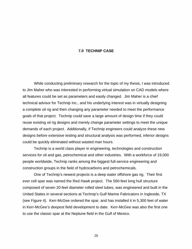
One of Technip’s newest projects is a deep water offshore gas rig. Their first
ever cell spar was named the Red Hawk project. The 560-feet long hull structure
composed of seven 20-feet diameter rolled steel tubes, was engineered and built in the
United States in several sections at Technip’s Gulf Marine Fabricators in Ingleside, TX
(see Figure 4). Kerr-McGee ordered the spar, and has installed it in 5,300 feet of water
in Kerr-McGee’s deepest field development to date. Kerr-McGee was also the first one
to use the classic spar at the Neptune field in the Gulf of Mexico.
26

Figure 4: Red Hawk model
Technip completed delivery of the Red Hawk in record time of 22 months from
contract award in September 2002. The design of the Red Hawk took approximately
57,000 man hours, half the time of previous designs (of comparable complexity)(see
Figure 5). They attributed this efficiency to three factors: keeping all the detailed
analysis work in one office instead of two, turning support structures from a ship type
structure into simple ring stiffeners, and turning complicated load cases into simple
governing criteria.
27

11 months
Figure 5: Gantt Chart of Original Red Hawk Project
In designs being created in the last three months, engineering design time has
been cut by another 50%. Complete designs for offshore oil and gas rigs over 500 feet
tall can be created in under 29,000 hours. This is now possible since Technip has
created global models that can be used as the base for each new project. The global
models can have any parameter changed quickly to meet the demands of each project.
One engineer can complete the drawings for a custom oil or gas rig in about 12 hours.
The final design just needs to be analyzed for static and dynamic loading. Now Technip
engineers are highly interested in what techniques are available to reduce their product
design time even further.
28

8.0 SOLUTIONS FOR TECHNIP
Managers at Technip were interested in trying new creative ideas for saving time
in product design, so I evaluated tools that could meet their demands and recommend
specific strategies for them to follow. With this very interesting dilemma, I began
evaluating possible solutions to meet their needs. My solution to their problem involved
a software package called DesignXplorer VT which was being developed by Ansys Inc.
I believed that this product showed significant promise for use in the Technip case. I
decided to evaluate to see if it would meet the needs of Technip.
Once a potential case study was found, I created a case study that would be very
relevant to Technip. Therefore, I selected components from the Red Hawk project to
use as a proof of concept test. I modeled an entire bulk head in Autodesk Inventor for
this test (see Figure 6). Inventor was used because it is the primary CAD software used
by Technip engineers. With this package I created CAD assembly drawings of a bulk
head that mimicked the ones used on the Red Hawk oil rig. I also set key geometry
dimensions as parameters which could be changed later.
29

Figure 6: Bulk Head model in Autodesk Inventor
Next, the completed CAD model assembly was then imported into Workbench
through Design Modeler. In Design Modeler, the mid-surfaced tool was used so that the
structure could be analyzed with shell elements, instead of the default solid elements.
Figure 7 shows a view of the mid-surfaced bulk head. Shell elements are more
accurate for solving models like this where pressure is the main loading.
30

Figure 7: Mid-surfaced Faces
I assisted Ansys Inc. in the development of the mid-surface feature through
testing and soliciting customer feedback. The mid-surface feature was not available
when I started development. My work with this project helped determine and correct
bugs that tool would cause the mid-surface feature to fail. I was able to report these
bug and recommend solutions to developers.
The bulk head model that I created for this project also became a benchmark test
for Ansys Workbench Mesher. The mesher was initially unable to process some of the
complex features in the model I created. By submitting this model to Ansys as a
benchmark test, I was able to work with developers to improve the capability of the
Workbench mesh tools to handle this model. Processing this model in the Workbench
mesher was an important priority for Ansys developers because the model was a good
representation of parts that Ansys customers would need to analyze on a regular basis.
Solving issues with model would immediately help other Ansys customers that have
similar problems.
When the simulation was complete, the model was run in Ansys DesignXplorer. I
decided to evaluate Ansys DesignXplorer because it was ideal for reusing existing oil
and gas rig designs and merely changing parameter settings to meet the unique
31

demands of each project. DX-VT analyzed several key geometry parameters, such as
wall thickness or size of support structures, to optimize the model for the most important
response parameters. One optimizing goal, for example, involved minimizing the
thickness of the inner bulk head supports, known as web stiffeners, until an idea max.
principle stress was obtained. Goal driven optimization became very quick and helpful
to perform tests like this because one solution already solved for all these possible
scenarios.
When all the analysis was completed, all the steps were captured to explain how
to repeat the process. Therefore I took procedure and made it into a best practice guide
for Technip engineers to follow (see Appendix A). The guide that shows the easiest
way for Technip, or any company needing to reduce product development time, to
virtually prototype and optimize designs with DesignXplorer software. This
demonstration shows how to design and test components for their oil rigs in a new and
innovative fashion. This best practice guide is accompanied by three interactive
demonstrations which go step by step to show how a Technip product can be analyzed
with FEA and CAE simulations to find weak points and recommend design changes to
better meet there performance needs.
The best practices guide was created to be a general guide on how to efficiently
use Workbench Design Modeler, Simulation, and DesignXplorer for enhancing product
development. This guide was tailored to Technip Inc. and their most recent project, the
Red Hawk. The best practices guide demonstrates how to use the Ansys Workbench
software to simulate actual components from the Red Hawk oil rig. The guide shows all
the steps and features that were required to get this complicated model to solve
properly.
I distributed the best practices guide to engineers at Technip, and shortly
thereafter went to Technip’s main US office in Houston, TX to train engineers on how to
use DesignXplorer, and its advanced features. While there I also made a proposal on
the value of Workbench and DesignXplorer, and how Technip will prosper from using
these tools. The training was well received by the Technip engineers. And they called
the best practice guide “invaluable” for getting them up to speed with the new
Workbench tools. After the training onsite in Texas, I have been frequently consulted as
32

a technical support advisor to the Technip engineers. They have asked me for dozens
of recommendations on how to best perform specific tests that they want to analyze.
My recommendations come from my experience and from suggestions of the Ansys
development staff, and have always proven useful to Technip.
Because of my link between Technip and Ansys, Technip engineers have
become beta testers of Ansys products. And this has proven to be a good relationship
because of how Technip pushes the software to its limits with large models, extensive
parameters, and heavy use of advanced functions. All these tough requirements from
Technip have given Ansys a clear understanding of what their customers demand from
their products. Having customers work so closely with the development of Ansys
products has been a huge help for driving the products success.
The interaction that I have made with Technip and Ansys has benefited both
companies. Technip has had a chance to pursue new product development techniques
that are very innovative for their type of products. While Ansys has seen a closer look
at what their customers software needs are. This interaction has provided active
feedback for Ansys on how there newly developed tools are working for their customers.
Technip continues to be a beta tester of the newest Ansys features, and this
relationship will hopefully last in the future to benefit both companies.
33

9.0 CONCLUSION
Through my work on the project, Technip is trying to implement DesignXplorer
VT in an effort to save 40% on design time. Based on the average salary for structural
engineers, this savings would account for up to $750K per project. DesignXplorer VT is
will be able to save time by automating repetitive processes required to do a simulation.
Also, savings will come from full integration with parameterized models from Autodesk
Inventor, where bi-directional associativity is possible. Figure 8 shows the proposed
reduced time in production, from 22 months to 18.5 months. Figure 9 is more
impressive, because it shows the decrease in design time from 11 months to 6 months.
That equals a savings of 45%.
34

Figure 8: Gantt Chart of reduced production time
35

Figure 9: Reduced engineering and design time
Technip is currently evaluating how well they can integrate Ansys Workbench
products into their product development cycle. If they incorporate my proposed ideas,
Technip will be the first in their industry to implement this type of innovative solution for
reducing product development time. Technip recognizes opportunities for DX-VT in the
Accessories department, where add on features that go on top of the oil rig platform.
These accessories tend to be more unique and innovative, and would benefit greatly if
DX-VT could help shape their design. Also, the sizes of these accessories CAD models
are well suited for the capabilities of DX-VT, so they won’t overwhelm the program by
being too large.
Engineers who are already using Ansys Workbench and DesignXplorer at Technip have
learned how by using the best practice guide I created. They commented that the guide
proved “invaluable” in getting them up to speed with learning the program, and figuring
a step by step plan to get analysis done. The technical support that I have given to the
Technip engineers has been well appreciated, and definitely used. Previously my
technical support recommendations would come from my experience and from
suggestions of the Ansys development staff. Question that Technip engineers are
36

asking recently, are more difficult than I can solve. These days I resort to forwarding
questions directly to Ansys Tech-support group, who have more experience and more
personnel to handle Technip's advanced problems.
In the future, when Technip implements these tools, the company should make a
re-evaluation of how their product development process is performing. In a fast paced
company such as Technip, it can easily take three months or more to become familiar
with the DesignXplorer tools. Therefore, after a three month trial period Technip should
evaluate what the product development bottlenecks are at that point. They should
evaluate how productive DesignXplorer has been for them, and determine what other
road blocks are slowing their product development cycle. Streamlining their process will
give them a notable advantage in their industry.
37

APPENDIX
BEST PRACTICES GUIDE
DESIGN MODELER
To get started in Design Modeler, run ANSYS Workbench and choose open
“New Geometry” in the first screen (Figure 10). This will open a new instance of Design
Modeler. Go to the top toolbar and select File > Import External Geometry File >
(Figure 11). This Import External Geometry File will allow the user to import a desired
model from Autodesk Inventor or other CAD programs. Select the desired CAD model
and click OK. The part will not appear on the screen until the user clicks Generate Part
from the toolbar (Figure 12).
38

Figure 10: Ansys Opening Screen
Figure 11: Import External Geometry
39

Figure 12: Generate button
Mid-surface Extraction
Mid-surface Extraction can be used to create shell elements out of existing solid
elements. This feature is very common when analyzing medium to thin walled
structures such as pressure vessels. To use this feature in ANSYS Workbench 9.0, the
user must turn on Beta Features. This is done by going to Tools > Options > Common
Settings > User Interface > (Figure 13). Set Show Beta Options = Yes, and click OK
(Figure 14).
Figure 13: Options Button
40

Figure 14: User Interface Options
To use the Mid-surface tool, go to Tools > Mid-surface > (Figure 15). The mid-
surfacing features will come up in the lower left toolbox. For quick mid-surfacing of all
parts, use Auto Select (Figure 16). Auto Select will ask the user to set the minimum and
maximum thresholds for determining the min and max thicknesses of geometry surfaces
that will be mid-surfaced into planes. These thresholds are important so that
Workbench does not reduce a part into a plane in the wrong (probably perpendicular)
direction. Next, set Automatic Detection to: ON, and all relevant parts will be highlighted
with one side pink and the other side purple (Figure 17). Select generate part to finish
the mid-surfacing feature.
41
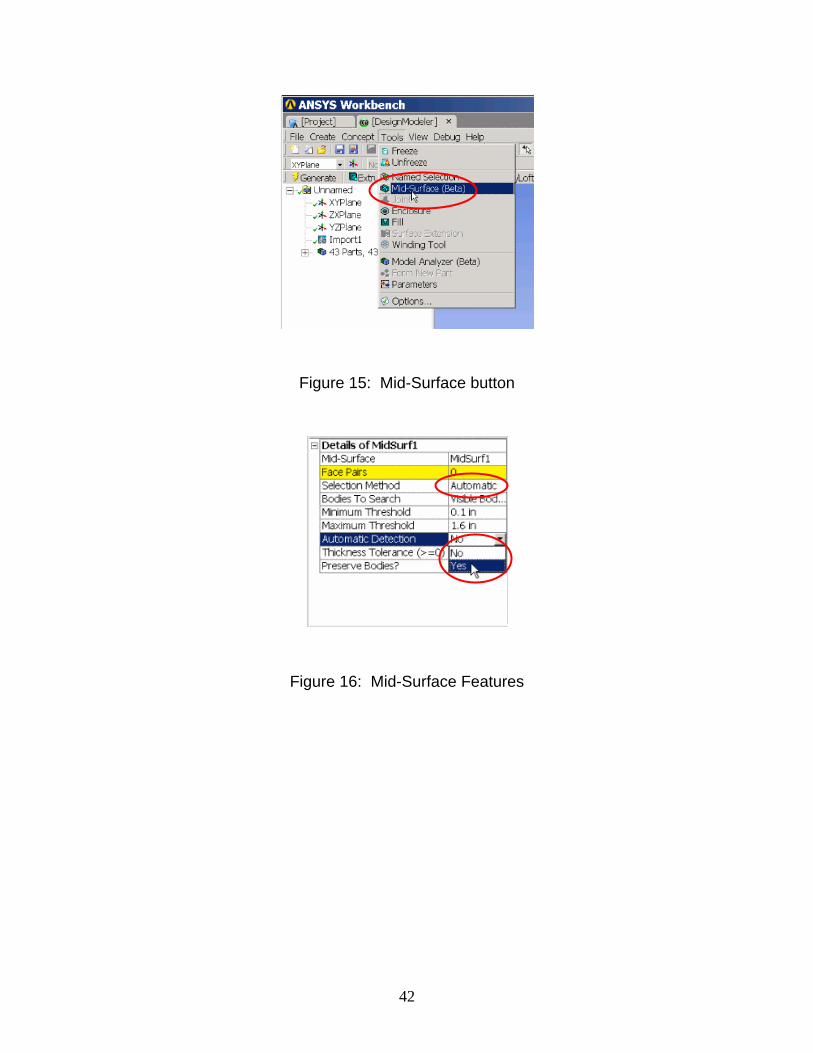
Figure 15: Mid-Surface button
Figure 16: Mid-Surface Features
42

Figure 17: Mid-surfaced Faces
Surface Extension
The Surface Extension tool is typically used after the mid-surface tool to correct
any gaps between joining surfaces where walls thinned to the mid section are no longer
touching joining surfaces, and a gap is created.
To use this tool, go to Tools > Surface Extension (Figure 18). The Surface
Extension features will come up in the lower left toolbox, where the user should click on
the Edge button (Figure 19). Next, select all edges that you wish to extend by holding
the Ctrl key and picking each edge from the geometry. It is also possible to select
multiple edges at once by holding the left mouse button down, and rolling over edges
that need to be selected. Now go back to the lower left toolbox, and select Apply on the
Edge to Extend feature. Set Extend to: To Surface (Figure 20). Then select all
surfaces to extend edges to, and then click the Target Face feature and hit Apply.
Finally, select Generate Part in the top toolbars.
43
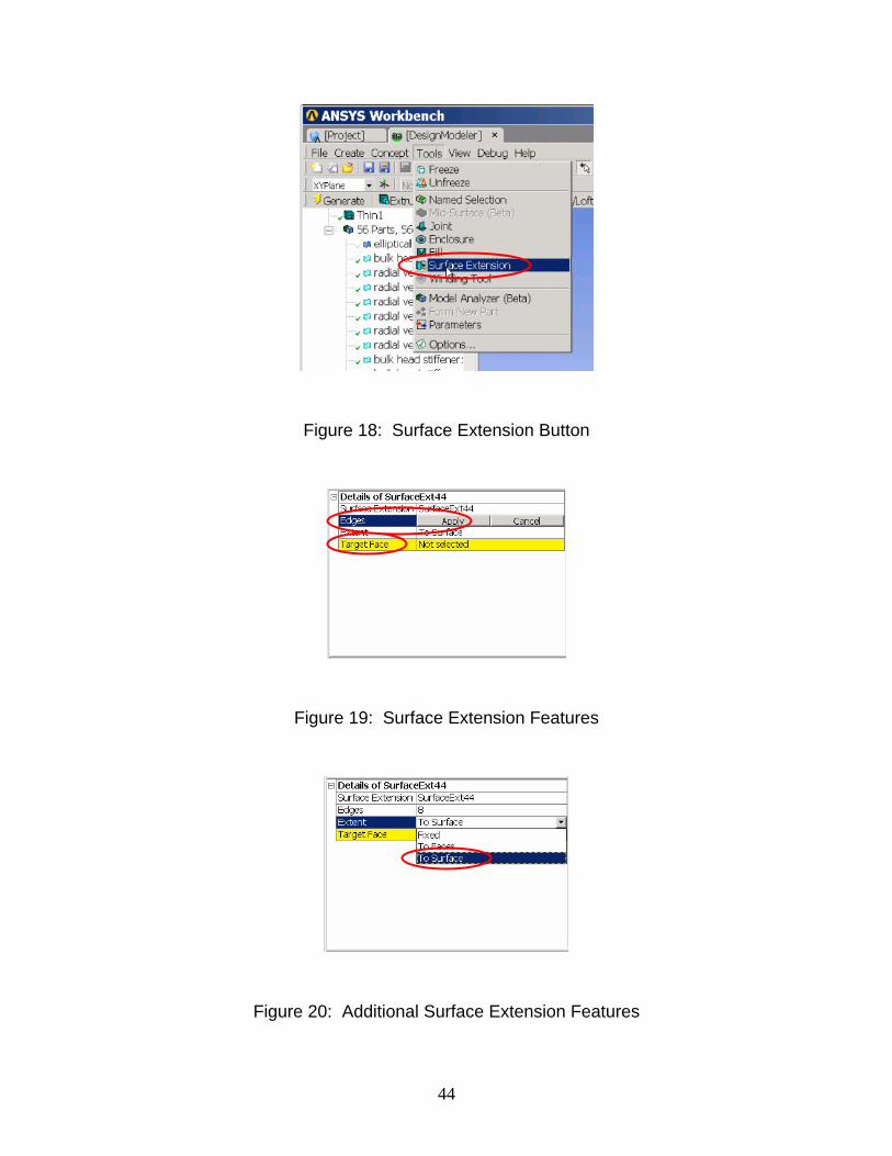
Figure 18: Surface Extension Button
Figure 19: Surface Extension Features
Figure 20: Additional Surface Extension Features
44

Thin Wall feature
The Thin Wall feature is used as an alternative operation if the geometry of a part
is too complicated for the Mid-surface tool to calculate. The Thin Wall feature reduces
the thickness of a solid part to zero. This allows ANSYS Workbench to think the solid
elements have no thickness, and can thus be treated as shell elements.
To use this Thin Wall feature, select the Thin/Surface button from the top toolbar
(Figure 21). Select the surface of geometry desired to make thin. In the lower left
toolbox change Thickness to equal zero (Figure 22). Select Generate Part in the top
toolbars to create this thin feature. This will allow parts to mesh as shell, and thickness
of shell can be determined later in simulation mode.
Figure 21: Thin/Surface Button
45

Figure 22: Thin/Surface Features
Joint feature
The Joint feature is a very helpful tool that can be used to join different parts, and
resolve possible contact problems in the simulation. If contact fails between two parts in
simulation, it might be useful to come back to Design Modeler and add joints between
the two parts. With a joint between parts, contact is not necessary to constrain these
parts to each other.
To use the Joint feature, go to Tools > Joint, and select Joint from the pull down
tab (Figure 23. In the lower left toolbox, select Target Bodies (Figure 24). Now
manually select all features that you wish to contain joints. Again, to select multiple
bodies at once, hold the left mouse button down and roll over edges that need to be
selected. Then select Apply in the Target Bodies area. All selected bodies that touch
another selected body will contain a joint at there intersection and the pair will have a
shared topology.
46
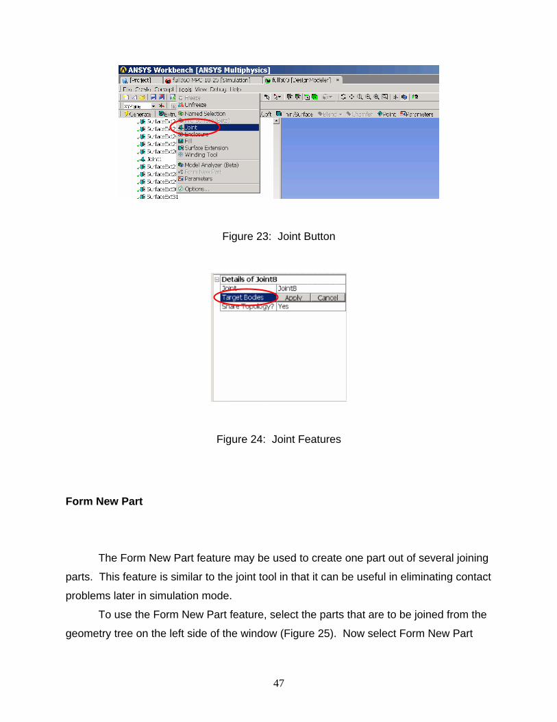
Figure 23: Joint Button
Figure 24: Joint Features
Form New Part
The Form New Part feature may be used to create one part out of several joining
parts. This feature is similar to the joint tool in that it can be useful in eliminating contact
problems later in simulation mode.
To use the Form New Part feature, select the parts that are to be joined from the
geometry tree on the left side of the window (Figure 25). Now select Form New Part
47

from Tools > Form New Part (Figure 26) after all the desired parts are chosen. A new
part will be automatically generated in the part tree.
Figure 25: Select Parts from Geometry Tree
Figure 26: Form New Part Button
48

Parameters
Parameters can be used to transfer changes in parameters from CAD program to
workbench. To make a geometry dimension or other design variable a parameters, in
the lower left window click the box to the left of each feature, which puts a “P” next to it
(Figure 27). These features will become parameters that can be varied in the
simulation or DX-VT mode.
Figure 27: Set Parameters
SIMULATION
Whence a Design Modeler file (.agdb) is created and saved, the next step is to
create a new simulation from the DM file. By going to the Project tab at the top of the
49

window, the user can click New Simulation to create new simulation from existing
geometry in the Design Modeler file (Figure 28).
Figure 28: Start New Simulation
Contact
Contact between all the bodies is automatically generated when the new
simulation is started. Although the automatic contact can be very thorough, it is
important to inspect the contact automatically selected. A good aid to this process is to
rename to contacts after the two bodies it refers to. Just right click on Contact in the
project tree on the left side of the window, and select Rename Based on Geometry
(Figure 29). Now go through the list and verify that contact between parts is correct.
50

Figure 29: Rename Contact Based on Geometry Button
There are two notable things to check for. First check that there aren’t duplicate
contacts. These are easier to find when the contact in names after the parts, and sorted
alphabetically. Delete duplicate contact regions (Figure 30). These contacts may have
been created because two bodies may have same edge-to-surface and surface-to-edge
contact point. It is only necessary to keep one of those contacts.
51

Figure 30: Deleting Duplicate Contact
The second thing to inspect the contact for is that correct parts are mating in
each contact pair. When contact is automatically generated Workbench uses a tool
called a “pinball” to determine which bodies should be in contact. Workbench puts two
bodies in contact if their distance apart is less than or equal to the size of the pinball.
However Workbench may not place contact between to bodies intended to be mating if
the gap between them is larger then the size of the pinball. The opposite of this is also
true, two bodies may be coincidently close together, but are mistakenly given a contact
point because their relation to each other was smaller than the pinball size. It is these
situations that the user needs to look for, and change the pinball size as necessary. To
change the pinball size, click on Contact in the project tree. Contact details will appear
in the lower left toolbox. The pinball size can be changed by entering a new value into
the Tolerance Value field (Figure 31).
52

Figure 31: Setting Contact Pinball Size
Another helpful tool for managing the contact for the simulation is the Contact
Tool. Simply right click on Contact in the project tree, and go to Contact > Insert >
Contact Tool (Figure 32). This tool gives the user a description of contact types, allows
user to change contact types, and allows user to delete inactive contacts (Figure 33).
All of which are good tools to use if the simulation fails for contact reasons.
Figure 32: Inserting Contact Tool
53

Figure 33: Deleting Inactive Contact
Material
Workbench offers several preset materials that can be chosen to represent each
part of the model. In addition, the user can specify the properties of their own material
they wish to use in their analysis. To select a material, click on geometry in the project
tree. Now highlight all the parts that will have the same material. Go to the lower left
toolbox, and click on Material. The user has the choice of selecting a predefined
material, creating a new material, or importing a material that has already been created
(Figure 34). The user should select one of these options for all the different parts in the
model. All parts need to be made of some type of material so that Workbench knows
how the material will react in the analysis.
Figure 34: Setting Material Properties
54

Meshing
A good mesh of the geometry can make all the difference in the world when
Simulation is trying to find a solution to the model. Key steps such as minimizing the
overall number of elements, refining the mesh around critical features, or mapping the
mesh with a standard pattern on simple bodies; all can have a large effect on the
success and accuracy of the solution. Several important modifications to the mesh will
be discussed here.
The first step for meshing is to allow Workbench to create a mesh for the user to
review. Use Preview Mesh to have Workbench generate a mesh of the model (Figure
35). For this, right click on Mesh in the project tree and click on Preview Mesh.
Workbench will automatically generate a mesh for the model based on preset criteria in
the mesher.
Figure 35: Preview Mesh Button
55

Whence the model is meshed, modifications can be made where the mesh is too
course or too fine. The tool for this is called Mesh Sizing. For this, right click on Mesh
in the project tree and click on Insert > Sizing (Figure 36). This tool refines the mesh on
selected bodies, surfaces, or edges; and makes the elements all roughly the size, which
the user specifies. The element size is set in the Element Size field in the lower left
toolbox (Figure 37). It is important to note that although this tool refines the mesh on
selected bodies, surfaces, or edges; using bodies for resizing tends to be more
successful when meshing solid bodies.
Figure 36: Insert Mesh Sizing
Figure 37: Mesh Sizing Details
56

Refinement is another tool that can be used to generally refine bodies or
surfaces to be meshed. This tool is helpful when a key feature or region wants to be
analyzed and the solution at these points needs to be most accurate and precise. To
use this tool, right click on Mesh in the project tree and click on Insert > Refinement
(Figure 38).
Figure 38: Insert Mesh Refinement
The Mapped Face Meshing tool is used to pattern the mesh in areas where the
geometry is simple and mesh symmetry is possible or preferred. Having a mapped
mesh makes the elements the same size and shape, and contain similar attributes. The
mapped mesh will also reduce the total number elements in most cases. These
features allow the Workbench solver to run faster, with less processing time required.
This feature is found under Insert > Mapped Face Meshing when one right clicks on
Mesh in the project tree (Figure 39).
57

Figure 39: Insert Mapped Face Meshing
Environment
The Environment of the simulation gives the model actions to react to. Actions
such as pressure, forces, acceleration, convection, heat flux, etc. can be used. In
addition the environment has the constraints that keep the model constrained in space.
Constraints such as fixed supports, frictionless supports, given displacements, etc. This
guide will focus on loads and supports that enable the user to do a structural analysis.
These features are only a small number of what is available in the environment section.
Loads can be inserted for the appropriate loading conditions of the model. When
doing a structural analysis, pressure loads on a surface give less local stress
concentrations then a force at a single point. To insert a pressure load right click on
Environment in the project tree, and go to Insert > Pressure (Figure 40).
58

Figure 40: Insert Structural Loads
Fixed Supports are necessary in a structural analysis to keep the model from
“flying away” when a force is applied to it. The user must insert appropriate supports to
keep model fully constrained. This is done by right clicking on Environment in the
project tree, and go to Insert > Fixed Support (Figure 41).
Figure 41: Insert Supports
59
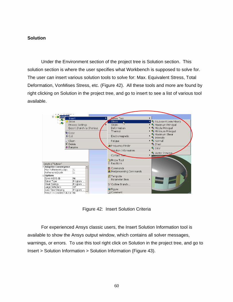
Solution
Under the Environment section of the project tree is Solution section. This
solution section is where the user specifies what Workbench is supposed to solve for.
The user can insert various solution tools to solve for: Max. Equivalent Stress, Total
Deformation, VonMises Stress, etc. (Figure 42). All these tools and more are found by
right clicking on Solution in the project tree, and go to insert to see a list of various tool
available.
Figure 42: Insert Solution Criteria
For experienced Ansys classic users, the Insert Solution Information tool is
available to show the Ansys output window, which contains all solver messages,
warnings, or errors. To use this tool right click on Solution in the project tree, and go to
Insert > Solution Information > Solution Information (Figure 43).
60

Figure 43: Insert Solution Criteria
Parameters
Parameters set in the Simulation stage of Workbench can be passed from
application to application within Ansys. The parameters allowable in Simulation include
CAD parameters and engineering parameters, such as dimensions of a part, geometry
mass, pressure, maximum stress, material properties, etc. To select parameters, there
is an empty box next to allowable parameters in the toolbox on the lower left side of the
window.
For example, to select a geometry parameter, go under the Geometry section of
the project tree, where each Geometry part is listed. Select a geometry part, and in the
lower left box there are geometry features. Click the box next to each geometry feature
that you wish to make a parameter (Figure 44). A “P” will appear in the box to show it is
set as a parameter. You may also select the box next to the solution criteria that you
with to optimize, such as shear stress, total deformation, etc. (Figure 45). A “P” will
appear in the box to show it is also set as a parameter.
61

Figure 44: Set Input Parameters
Figure 45: Set Output Parameters
62
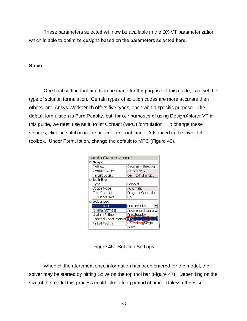
These parameters selected will now be available in the DX-VT parameterization,
which is able to optimize designs based on the parameters selected here.
Solve
One final setting that needs to be made for the purpose of this guide, is to set the
type of solution formulation. Certain types of solution codes are more accurate then
others, and Ansys Workbench offers five types, each with a specific purpose. The
default formulation is Pure Penalty, but for our purposes of using DesignXplorer VT in
this guide, we must use Multi Point Contact (MPC) formulation. To change these
settings, click on solution in the project tree, look under Advanced in the lower left
toolbox. Under Formulation, change the default to MPC (Figure 46).
Figure 46: Solution Settings
When all the aforementioned information has been entered for the model, the
solver may be started by hitting Solve on the top tool bar (Figure 47). Depending on the
size of the model this process could take a long period of time. Unless otherwise
63

specified, all analysis is done of the desktop computer where the Workbench software is
running. When the solution is finished, the used should review results for accuracy.
Solving a model is traditionally an iterative process where mistakes are found in the
solution, the input information (such as mesh detail) is corrected, and the solver is run
again.
Figure 47: Solve Button
When the solution for the model is reached, the user will be able to analyze all
the information that was solved for. Analyzing the areas of highest deflection (Figure
48) or stress (Figure 49) may prompt the designer to made design changes in those
areas of focus. Also, seeing areas of little deflection may prompt the user to subtract
material from over designed areas. If a user makes any changes to the model, they
would next re-run the simulation to verify that their changes produced acceptable
results.
64

Figure 48: View of Total Deformation Solution
Figure 49: View of Maximum Principle Stress Solution
65

Reports
A very nice feature that Workbench offers is the reports section. Workbench can
automatically generate a Design Report for the user, in which The Design Report shows
summaries of all parameters, design sets, and response charts saved as snapshots. To
generate a design report, click the Report Preview tab at the bottom of the main window
(Figure 50). You can also use Publish Report to write the report as an HTML file in a
designated directory.
Figure 50: Simulation Design Report
66

Decreasing Solving time
If the desktop computer where Workbench is installed is part of a larger Ansys
server, it is possible to run solutions on the server for faster processing. By going to
Tools > Options in the top toolbar, an Options window appears. Click on Simulation >
Solution to see where Workbench currently runs the Solver (Figure 41). In the right box
of this options window are settings to change the location of process settings. Change
these settings to the location of the server, and workbench will use that server for
processing the simulation analysis.
Figure 51: Solution Settings
67

DX-VT
DesignXplorer VT (DX-VT) is used for analyzing the response of parts and
assemblies in a simulation model. DesignXplorer was created from various optimization
methods such as Design of Experiments (DOE). Through these methods, DT-VT uses
parameters from Simulation, Design Modeler, and various supported CAD packages as
the inputs for solving an optimization. Input and response parameters are the main
variables used to find an optimal solution.
The variation technology in DesignXplorer VT helps provide a much more
efficient and timely solution to these problems. By using mesh morphing and the Taylor
series expansion approximation, DX-VT can provide a response surface that is based
on a single finite element solve. This is done by calculating the derivatives of the FEA
solve. The effect of this is an “extended” finite element analysis that takes longer than
one FEA solve, but is much shorter than the multi-solution runs that are required for a
regular DX solve.
8.3.1 Begin & Select Parameters
To run a DX-VT study, follow these steps: Begin by having a Workbench
Simulation session open with all the parameters specified. See Simulation- Parameters
above for details. Open a DX-VT study by selecting New DesignXplorer VT study from
the project tab in Workbench (Figure 42). When the DX-VT window opens, select the
input parameters from the left column that are important to this particular study (Figure
43). Input parameters normally include geometry dimensions, material properties, or
suppressed features. Response parameters are all included from those chosen in
Simulation, and could be parameters such as geometry mass, total deformation, shear
stress, etc.
68
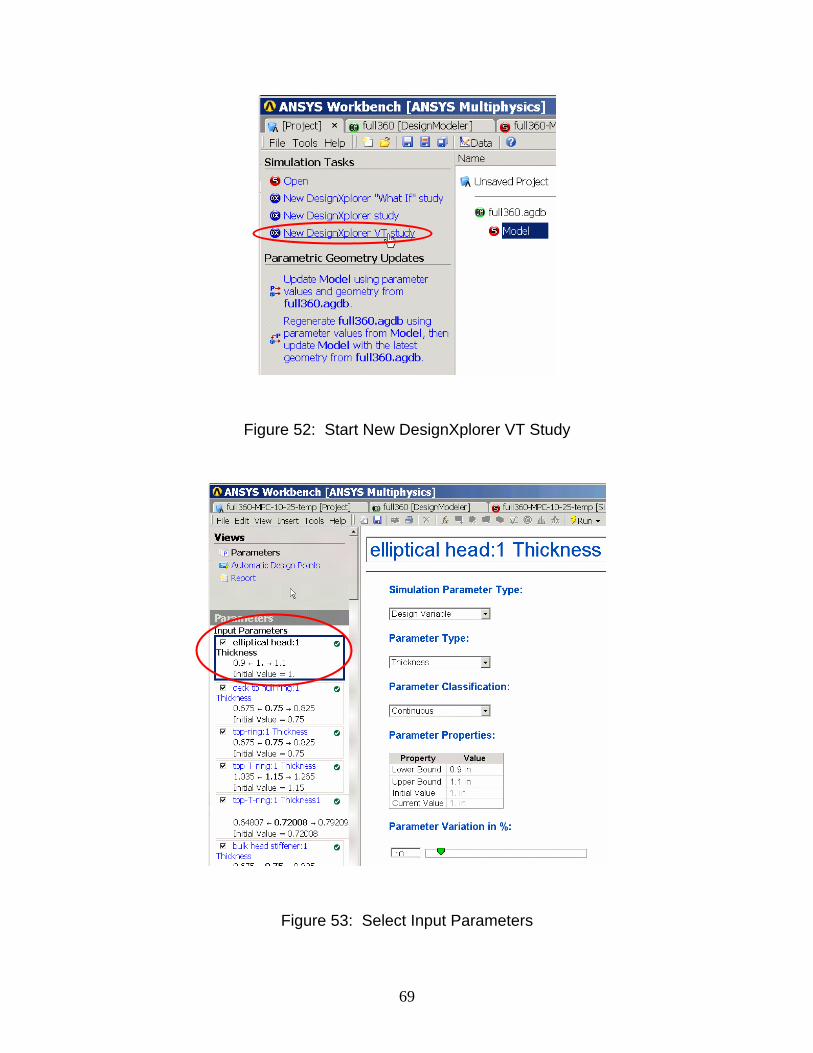
Figure 52: Start New DesignXplorer VT Study
Figure 53: Select Input Parameters
69

Define Parameter types
When selecting each parameter there are pull down tabs in the middle of the
screen to choose the proper Simulation Parameter Type, Parameter Type, and
Parameter Classification (Figure 44). The Simulation Parameter Type may a design
variable or uncertainty variable. Use design variable if you know the parameter is a key
part to the design. The Parameter Type (for geometry parameters) specifies how the
parameter is used in the part, length, angle, thickness, etc. The Parameter
Classification can be set to continuous (for continuous variation of value) or usability (for
discrete use or non-use of the parameter).
Figure 54: Parameter Details
70

Also in the main window as the last parameter setting is a place to change the
Parameter Variation. Changing this variation allows DX-VT to solve for a larger or
smaller range of values for that parameter. Larger variation ranges give more design
points to experiment with, but also increase the time it takes to reach a solution.
Run Solve in ANSYS
When the parameters are all selected and defined, run the DX-VT solve by going
to the top toolbar and selecting Run > Solve in ANSYS (Figure 45). This will perform
the ANSYS solve with variation technology so that one solution will be sufficient for
analyzing hundreds or thousands of design points.
Figure 55: Solve in ANSYS Button
Responses
After the solution has finished, new views will become available in the left column
of the window. The Response button on the left column (Figure 56) shows each
response variable, and allows the user to vary the input parameters by moving the slider
bar between the extreme points of that particular study (Figure 57). The response
variable changes as the input variable is adjusted. This change can be seen in the
graphical display of the assembly on the main section of the window.
71

Figure 56: Responses Button
Figure 57: Response to Input Parameters
72

Goal Driven Optimization
By using Goal-Driven Optimization (GDO), DesignXplorer will create multiple of
robust design points through sample generation. To generate samples, pick or enter
the number of samples in the Sample Generation box in the lower left part of the
window (Figure 58). Sample size should be based on complexity of analysis, the more
complex the model, the longer it will take to generate these samples from the solution
data. Therefore it might be time efficient for a larger model to have less samples. A
good size for completeness is 1000 samples, if the model if moderately complex (under
20,000 elements).
Figure 58: Sample Generation
The next step is to set Goals for Input and Response Parameters. In the main
window, click on each parameter that needs to be optimized in this study (Figure 59). In
the row of each parameter there are pull down lists to set Desired Value and Importance
for each parameter. In the Response Parameters a target value can also be set, which
can be very useful for certain goals such as target mass, etc (Figure 60). When all the
73
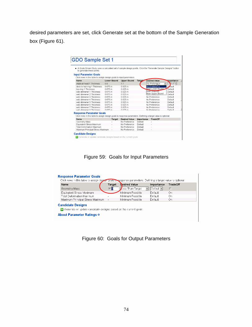
desired parameters are set, click Generate set at the bottom of the Sample Generation
box (Figure 61).
Figure 59: Goals for Input Parameters
Figure 60: Goals for Output Parameters
74

Figure 61: Sample Generation Button
When the samples have been generated click on the button under Candidate
Designs at the bottom of the main window (button reads: Generate or update designs
based on current goals) (Figure 62). Under Candidate Designs, three candidates will be
generated that rank best with the goals selected for this sample. The candidates have
each parameter listed with a number of stars or X’s bases on how well or poor each
parameter came to meeting the goal set. Choose a Candidate Design with the most
acceptable parameter attributes (Figure 63). Insert selected candidate as a soft design
by clicking the button labeled: “Insert selected as a soft design” at the bottom of the
main window (Figure 63).
Figure 62: Candidate Designs
75

Figure 63: Best Candidate Designs
Sensitivities
Under the Goal Driven Optimization bar in the left column, click Sensitivities
(Figure 64). This feature shows charts of significant input parameters. The charts show
how significant each input parameter is on any response parameter such as Total
Deformation. Click the different response parameters at the bottom of the left column to
see what input parameters affect the response parameters and by how much.
76

Figure 64: Sensitivities
Trade off study
The Trade Off Study allows the user to explore the calculated response surface
of a response variable based on two competing input variables. By selecting two
competing input and one output parameter in the left column, the main window will
display a 3D plot of input and response parameters (Figure 65). The chart shows
sample input parameters values, and the response parameters values, which is useful
to show where response parameters reach a min, max, or more importantly inflection
point. For example, this chart would help find the ideal input parameter values to
minimize Max Principle Stress.
77

Figure 65: Tradeoff Plot 3D
Reports
DesignXplorer offers a sophisticated reports section similar to those produced by
Workbench Simulation. DX-VT automatically generates a Report for the user that
summarizes: Design Parameters, Min/Max Search Results, Design Goals, Custom
Design Points, Automatic Design points, Responses, Sensitivities, Goal Driven
Optimization Sets, and Trade-off Studies to name a few. To generate this report, click
the Report button on the left column of the window (Figure 66).
78

Figure 66: DX Reports
79

BIBLIOGRAPHY
[1] Crabb, H.C. 1997. The Virtual Engineer: 21st Century Product Development. Society of Manufacturing Engineers, MI.
[2] Roth, G. Analysis In Action: The Value of Early Analysis, 7 Jan. 2005. Ansys Inc.
<http://www.ansys.com/assets/white-papers/wp_eaton.pdf> [3] Hopp, W.J., Spearman, M.L. 2001. Factory Physics: Foundations of
Manufacturing Management. McGraw-Hill, Inc., NY. [4] Ulrich, K.T., Eppinger, S.D. 1995. Product Design and Development. McGraw-
Hill, Inc., NY. [5] Chua, C.K., Leong, K.F. 1997. Rapid Prototyping: Principles & Applications in
Manufacturing. John Wiley & Sons (Asia) Pte Ltd, Singapore. [6] Leveraging Simulation: The Design Innovation Process, 7 Jan. 2005. Ansys Inc.
<http://www.ansys.com/assets/white-papers/wp_innovation.pdf> [7] Widas, P. Introduction to Finite Element Analysis, 8 Apr. 1997. Virginia Tech
Material Science and Engineering. <http://www.sv.vt.edu/classes/MSE2094_NoteBook/97ClassProj/num/widas/history.html>
[8] Enterprise-Wide Solutions: Product Design, Analysis, and Management Through
Engineering Teamwork, 7 Jan. 2005. Ansys Inc. <http://www.ansys.com/assets/white-papers/wp_ews.pdf>
[9] Thomke, S. "Enlightened Experimentation: The New Imperative for Innovation"
Harvard Business Review, Feb. 2001. [10] Urban, G.L., Hauser, J.R. 1993. Design and Marketing of New Products, 2nd
Edition. Prentice-Hall, Inc., NJ. [11] Reinerten, D.G. 1997. Managing the Design Factory: A Product Developer’s
Toolkit. THE FREE PRESS, NY.
80


![Andrew Martin - The 'X-rated' Albin Counter-gambit [Chess]](https://img.pdfslide.net/doc/110x75/55cf9dad550346d033aeaba0/andrew-martin-the-x-rated-albin-counter-gambit-chess.jpg)