Embed Size (px)
Citation preview
0
Time Series Momentum and Macroeconomic Risk
Mark C. Hutchinson Department of Accounting, Finance & Information Systems
and Centre for Investment Research University College Cork
College Road, Cork, Ireland. Tel +353 21 490 2597
Email: [email protected]
John O’Brien Department of Accounting, Finance & Information Systems
and Centre for Investment Research University College Cork
College Road, Cork, Ireland. Tel +353 21 490 1850 Email: [email protected]
This Version: 18th August 2015
JEL Classifications: G10, G19
Keywords: Time Series Momentum, Macroeconomic Risk, CTA
We are grateful to Nick Baltas, Jasmine Fang, David F. McCarthy and participants at the 2015 FMA Venice conference for helpful comments. We would also like to thank Aspect Capital Limited for financial support.
1
Time Series Momentum and Macroeconomic Risk
The time series momentum strategy has been shown to deliver consistent profitability over a long time horizon. Funds pursuing these strategies are now a component of many institutional portfolios, due to the expectation of positive returns in equity bear markets. However, the return drivers of the strategy and its performance in other economic conditions are less well understood. The authors find evidence that the returns to the strategy are connected to the business cycle. Returns are positive in both recessions and expansions, but profitability is especially high in expansions. About 40% of returns are due to time varying factor-related risk exposure, consistent with rational asset pricing theories having a role in explaining the profitability of the strategy.
2
1. Introduction
Subsequent to strong performance in the 2008 financial crisis Commodity Trading
Advisors (CTAs) pursuing time series momentum strategies have experienced large inflows
and are now a feature of many institutional investor portfolios.1 For many investors the
intuition behind including CTAs in their portfolio is primarily the expectation of high
performance during equity bear markets.2
Though choosing a strategy due to an expectation of positive performance during
these periods is reasonable, it disregards the drivers of profitability of the strategy and may
convey the idea that high returns are exclusive to equity bear markets. Unlike traditional asset
classes or other hedge fund strategies, there is scant academic evidence to date on the
interaction between the returns of time series momentum and the business cycle. While the
academic literature does show that the strategy has historically generated consistently
positive returns, and that at least a portion of time series momentum returns are due to
behavioural factors, it is a common sentiment amongst investors that performance is equity
market period specific.
In our paper, to help investors understand the drivers of profitability, we explicitly test
the connection between time series momentum strategies and the business cycle. We arrive at
four key findings. First, time series momentum portfolio returns exhibit statistically
significant differences across the business cycle. While positive in both, typically the
performance of the portfolio is higher in economic expansions than recessions. Second, we
show that though a linear macroeconomic factor model has little explanatory power, a model
which allows the coefficients to vary through time, does result in several of the
1 According to data from Barclayhedge as of the 3rd Quarter of 2014 CTA assets under management (AUM) was $312.6 billion. 2 See, for example, “Global worries forecast to boost flow of assets”, Financial Times, June 9th 2012.

3
macroeconomic factors having a statistically significant relationship with time series
momentum. Third, we show that when time series momentum portfolios are formed on either
the factor-related or asset-specific portions of financial futures returns they generate
statistically significant excess returns in both cases, with about 40 percent of returns coming
from the factor-related portion. Finally, using a new estimation approach, we find that time
series momentum generates higher returns in periods when economic uncertainty is lower.
From a practitioner’s perspective, these results show that there is a role for rational
asset pricing in explaining at least a portion of the returns to time series momentum; the
strategy is related to macroeconomic risk factors which have previously been shown to be
important in explaining the returns of both traditional and hedge fund portfolios; and perhaps
most importantly, our evidence points to how practitioners can expect performance to vary
across different future macroeconomic environments. In the next section we review the
related literature and discuss how our results link to and extend this literature.
2. Literature review
The literature on time series momentum is typically focused on the performance of
different variations of these strategies for particular markets in specific periods (see for
example Erb and Harvey (2006), Miffre and Rallis (2007) and Fuertes et al. (2010) for
commodities, and Okunev and White (2003) and Menkhoff et al. (2012) for currencies). The
evidence of these studies is generally positive on the performance of time series momentum
with positive Sharpe ratios and little correlation with traditional asset classes. Our paper
compliments Moskowitz et al. (2012) who introduce multi asset class time series momentum
to the literature. In a comprehensive study Moskowitz et al. (2012) investigate how time
series momentum relates to market movements, sentiment, and the positions of speculators;
finding evidence supporting a behavioural explanation for time series momentum
4
profitability. Our study builds upon Moskowitz et al. (2012) in that we focus on
macroeconomic factors which have been shown to be important for hedge funds and
traditional portfolios, employ methodologies which directly incorporate time variation in
factor exposures, and provide evidence that rational asset pricing may also be important in
explaining returns.
Recent evidence linking time series momentum and the broader macroeconomy
(Hutchinson and O'Brien (2014)) shows that following each of the six largest financial crises
in the last hundred years, there was an extended period where time series momentum
performance was below average. Though Hutchinson and O'Brien (2014) suggest several
explanations why the performance of the strategy might differ in different economic
conditions, unlike our study, they provide no empirical evidence connecting the strategy to
the business cycle. The present paper also addresses a gap in Hutchinson and O'Brien (2014)
by identifying the link between the business cycle and their finding that time series
momentum tends to perform below average following periods of financial crisis. Using a new
methodology, we document that uncertainty around changes in macroeconomic factors is the
transmission mechanism linking the below average returns following large global financial
crises and the business cycle.
By finding a link between the macroeconomy and time series momentum in a time
varying framework we build upon several related papers on time series and cross sectional
momentum.3 The cross sectional momentum literature finds a strong relationship between
macroeconomic factors and returns (Chordia and Shivakumar (2002)). While, to date, no one
has considered this specification for time series momentum, related literature has
3 As noted by Moskowitz et al. (2012) cross sectional momentum and time series momentum are related but different strategies. The key difference being that cross sectional momentum trading decisions are based upon the historical return of a security relative to other securities, whereas time series momentum is based upon the historical return of a security, considered independent of other securities. See Goyal and Jegadeesh (2015) for a decomposition of both strategies.
5
demonstrated the lack of explanatory power for a range of traditional factors in a linear
framework (Menkhoff et al. (2012) and Moskowitz et al. (2012)).4 We find that the
relationship between returns and macroeconomic factors is only revealed in a model which
explicitly allows for time varying exposure to risk factors. However, our conditional model
results show that a significant portion of time series momentum returns are not explained by
the macroeconomic factors.
Within the cross sectional momentum literature Conrad and Kaul (1998) argue that
profitability is due to differences in cross sectional expected returns. Illustrating this, Chordia
and Shivakumar (2002) demonstrate that when the returns of the underlying equities into are
divided into macroeconomic factor-related and asset-specific components, the majority of
cross sectional momentum profitability comes from the portion of equity returns explained by
macroeconomic factors. Contrary to this, in the first study to consider the returns of time
series momentum from this perspective, we find that the returns to our portfolios are
attributable to both the asset-specific and factor-related components of financial futures.
More recently, the hedge fund literature has linked the performance of a range of
hedge fund strategies to economic uncertainty. Bali et al. (2014) find that the sensitivity of
hedge funds to uncertainty about the economy is important in explaining the cross sectional
deviation in their performance. In the first study to apply this methodological approach to
time series momentum, our evidence suggests that time series momentum returns tend to be
higher when economic uncertainty is lower than average.
3. Data and methods
4 We acknowledge that the broad range of drivers of returns investigated by Moskowitz et al. (2012) do relate to time variation in strategy performance.
6
In this section we describe the selection of the sample period and the data used in the
analysis. The dataset consists of individual exchange traded futures contracts, synthetic
forward contracts and a range of macroeconomic variables.
3.1 Futures data
In this paper we investigate the relationship between macroeconomic variables and
the returns of the time series momentum investment strategy. As consistent monthly
macroeconomic data only becomes available from the late 1940s, we specify January 1950 as
the starting point for the analyses.5 The sample period runs to the end of September, 2014.
We split the sample into two sub-periods, January 1950 to December 1979 and January 1980
to September 2014, based around the peak of the great inflation. The first period is
characterised by high inflation and increasing interest rates, whereas from 1980 inflation fell
quickly and remained in a range of 2% to 5% for most of that period.6 In this second sub-
period interest rates fell steadily, from a high of 15.5% in 1981 to a low of 1.7% in 2012.7
Dividing the sample into these two sub-periods allows us to assess performance in different
long term interest rate cycles.
The futures data set consists of twenty one commodities, thirteen government bonds,
twenty one equity indices and currency crosses derived from nine underlying rates covering
the period from January 1949 to September 2014. The data consists of a combination of
exchange traded futures data and forward prices derived from historical data. The momentum
signals and portfolio returns are based on continuous return series. Using only exchange
traded futures contracts would limit the time frame of the study to post-1980. In order to
extend the study period backwards we follow the methodology used in other long term
5 We also use data for the twelve months prior to January 1950 to generate trading signals for the initial time series momentum portfolios. 6 Annual change in US CPI, source Federal Reserve Economic Database. 7 US Treasury 10 Year yield, source Federal Reserve Economic Database.

7
studies of time series momentum (see, for example, Hurst et al. (2012)) and combine
exchange traded prices with synthetic forwards created from the underlying instruments.
Exchange traded futures’ prices are available from Datastream from 1980 to the present. Prior
to this period, we obtain continuous return series for commodity futures from Commodity
Systems Inc. and MSCI currency data from Datastream. All older data is sourced from Global
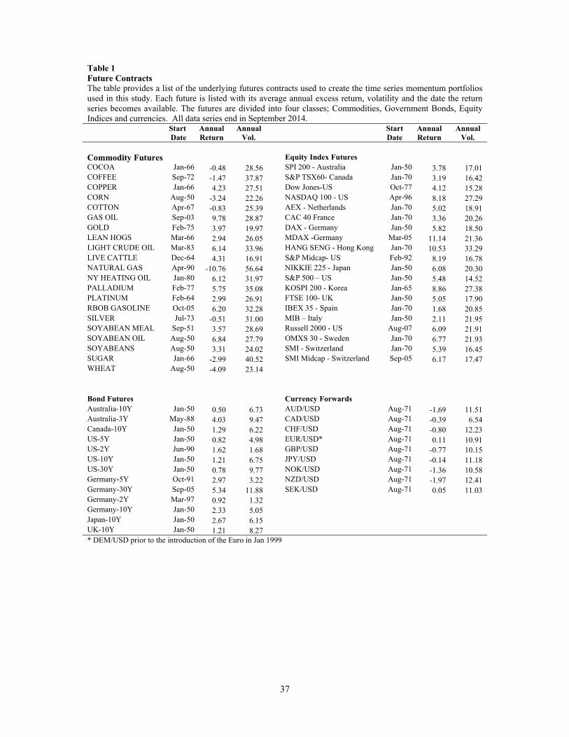
Financial Data. Table 1 shows a full list of the futures used in the study and data sources are
discussed in greater detail in Appendix A.
[Insert Table 1 here]
Where a futures contract trades on an exchange, the return series of the individual
futures contracts are combined to produce a continuous excess return series. Where futures
contracts are not available, forward prices are created by combining the underlying spot
price, yield and risk free rate. These two approaches are discussed below.
Continuous returns from futures contracts
Continuous return series are created from futures where daily price and volume data is
available. We calculate the daily excess return of the most liquid contract. This is generally
the front month or the next-nearest to delivery month. We select the most liquid contract as
follows. At time, t, the average volume over the previous three trading days is measured for
each of the live delivery dates. We select the contract with the highest volume to be recorded
as the excess return for that day. To replicate the practicalities of rolling contracts, once we
select a further delivery month, we do not allow the excess return of nearer delivery months
to be selected again.
Continuous return forward prices
8
Where exchange traded futures are not available, excess return series are created from
the underlying spot price, risk free rate and yield. The excess return from buying a forward at
the start of a month and holding it to month end, , is given by:
1/
1 (1)
where is the spot price return for the month, is the one month risk free rate, and is the
annualized yield. In order to confirm the validity of using synthetic forwards, a number of
tests were carried out where exchange traded futures returns were replaced by synthetic
forward returns. The series were typically almost perfectly correlated and in all cases results
were close to identical.
3.2 Economic data
Recent evidence has documented a strong link between macroeconomic risk and
hedge fund strategies (Bali et al. (2014)). Due to the power of these factors for hedge funds
we specify the economic factors presented in Bali et al. (2014) for all analyses.8 Consistent
with Bali et al. (2014) we use the Federal Reserve Economic Database, the Bureau of Labour
Statistics and the online data libraries of Robert Shiller and Kenneth French for economic
data. A more detailed description of the sources can be found in Appendix A. Information is
available for all eight factors from January 1950 to September 2014. We also examine the
performance of time series momentum portfolios in periods of economic expansion and
recession, based on definitions from the National Bureau of Economic Research (NBER) and
GDP data from the Federal Reserve.
3.3 Time series momentum portfolio
8 For robustness we also conducted all analyses using Chordia and Shivakumar (2002) and Chen et al. (1986) factors. The results (unreported) for all analyses, with the exception of economic uncertainty, were stronger with these alternative specifications.

9
The analyses of time series momentum in this paper are based on time series
representing the performance of the strategy across four distinct asset class sub-portfolios and
a diversified portfolio combining the four sub-portfolios.
The portfolios and their associated return series are created from the excess returns of
the instruments in the data universe. Where possible, excess returns are taken directly from
futures contracts trading on public exchanges, with the return of the most active contract,
defined as a function of trade volume, used as the excess return. Where futures exchange data
is not available for earlier periods, synthetic forward prices are created by combining the
underlying spot price, yield and risk free rate.
In creating the time series of time series momentum portfolios we use a twelve month
formation (look-back) period and a one month holding period.9 These are the most common
definitions used in the literature (see, for example, Hurst et al. (2012), Moskowitz et al.
(2012) and Baltas and Kosowski (2013)). The first step is to assign each instrument a
momentum signal, defined as
, ∑ log 1 (2)
Where, , is the momentum of instrument i at time t formed with a look back
period of k months and is the excess return of instrument i at time t - k.
The instruments are divided into four asset classes, Equity Indices, Government
Bonds, Foreign Exchange and Commodities and a time series momentum portfolio is created
for each class. Each instrument is given a weight proportional to its momentum signal and
inversely proportional to its volatility, so the size of the position is
9 Repeating the analyses using a range of different parameters, including the momentum signal defined in Hutchinson and O'Brien (2014), produces very similar results.

10
. (3)
Where is the weight of instrument i held in the portfolio at time t and is the
corresponding volatility. is the number of instruments in the asset class. This adjusts the
weights so that each sub-portfolio is allocated the same level of risk irrespective of the
number of assets in the class.10 The position is scaled by Vo, the choice of this is arbitrary, but
is set at 40% so the resulting return series have volatility levels in a range from 10% to 15%,
equivalent to those reported in the literature, allowing easier comparison (Moskowitz et al.
(2012)). The portfolio is rebalanced monthly11 so the return series for each sub-portfolio is
∑ . (4)
Where is the excess return of sub-portfolio c in time period t. The time series for
the diversified portfolio is the sum of the return series of the four sub-portfolios.12
Ex-ante volatility
We replicate the methodology of Moskowitz et al. (2012) to create the ex-ante
volatility estimates. This method uses an exponentially weighted squared daily returns model
to estimate volatility, a model similar to a univariate GARCH model. The annualised
volatility for each instrument is calculated as:
261∑ 1 (5)
The parameter is chosen so that the center of mass of the weights is 60 days, so data
from the last sixty days carries equal weight to all data up to then. The same model is used for
all instruments.
10 Risk levels are not exactly matched as we do not include correlation between assets. 11 The portfolio construction does not allow for intra-month changes in volatility. 12 In periods where there are fewer than four portfolios, returns are scaled so the diversified portfolio has constant target volatility throughout the entire sample period.
11
Transaction costs are included in the performance measures in this paper, using the
cost model described by Hurst et al. (2012), where costs are a function of asset class and
time. All returns presented are in excess of the risk free rate. In general results are presented
for three time periods: the entire sample period, January 1950 to September 2014; and two
sub-periods, January 1950 to December 1979 and January 1980 to September 2014.13
The cumulative excess return of the diversified portfolio is shown in Figure 1 and the
summary performance statistics for the diversified portfolio and the four asset class sub-
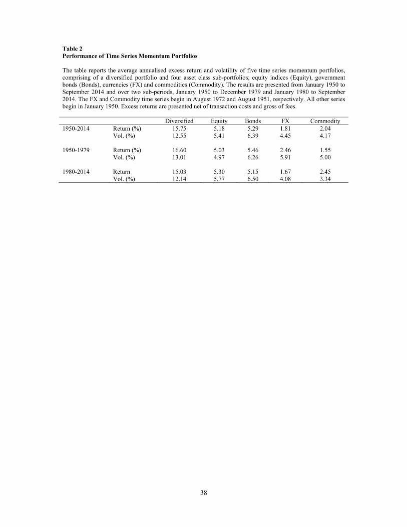
portfolios are presented in Table 2.
[Insert Figure 1 here]
[Insert Table 2 here]
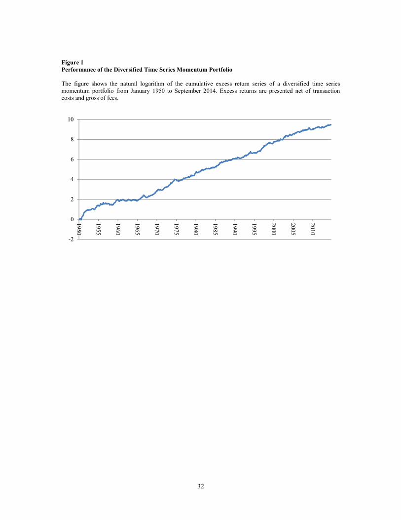
The most striking feature is the consistent excess returns generated by the time series
momentum strategy in the long run. The diversified portfolio and all sub-portfolios are
positive over the full period and both sub-periods. Over the full sample the diversified
portfolio generates a mean annualised excess return of 15.75% with a volatility of 12.55%
which translates into a Sharpe ratio of 1.25. The pattern of strong positive returns is
consistent with studies of time series momentum strategies by Moskowitz et al. (2012) for the
period 1985 to 2009 and Hurst et al. (2012) who examine an extended period from 1903 to
2012. It is also notable that there is little difference in performance for the diversified
portfolio or the Bond sub-portfolio between the two sub-periods, despite the dramatically
different interest rate regimes.
4.0 Time series momentum across the economic cycle
13 FX results do not begin until August 1972, so results reported for this asset class in the earlier sub-period are based on a relatively short sample period.
12
To examine the performance of time series momentum across the economic cycle, we
initially measure and compare the performance of time series momentum in different
economic states. The states are defined as a function of an economic or interest rate spread
variable. Each month’s return is assigned to one of the two possible states. The average
performance of the strategy in each state is calculated as the annualised mean of the pooled
excess returns for that state.
The variation in performance of time series momentum under different economic and
interest rate spread states is analysed here, first for the business cycle using two different
definitions of recession, and then by using interest rate spreads (term and default) to define
the state.
Economic states
The variation in performance of time series momentum under different economic
conditions is tested by splitting the return of the time series momentum return series
according to the contemporaneous economic state. The economy is allowed to be in one of
two states, expanding or contracting. Two definitions of economic state are used. The first
uses NBER recession definitions to define the state of the economy as contracting, with all
other periods defined as expanding. The second uses the sign of the change in GDP to define
the economic state; a positive change corresponded with an expansion and a negative change
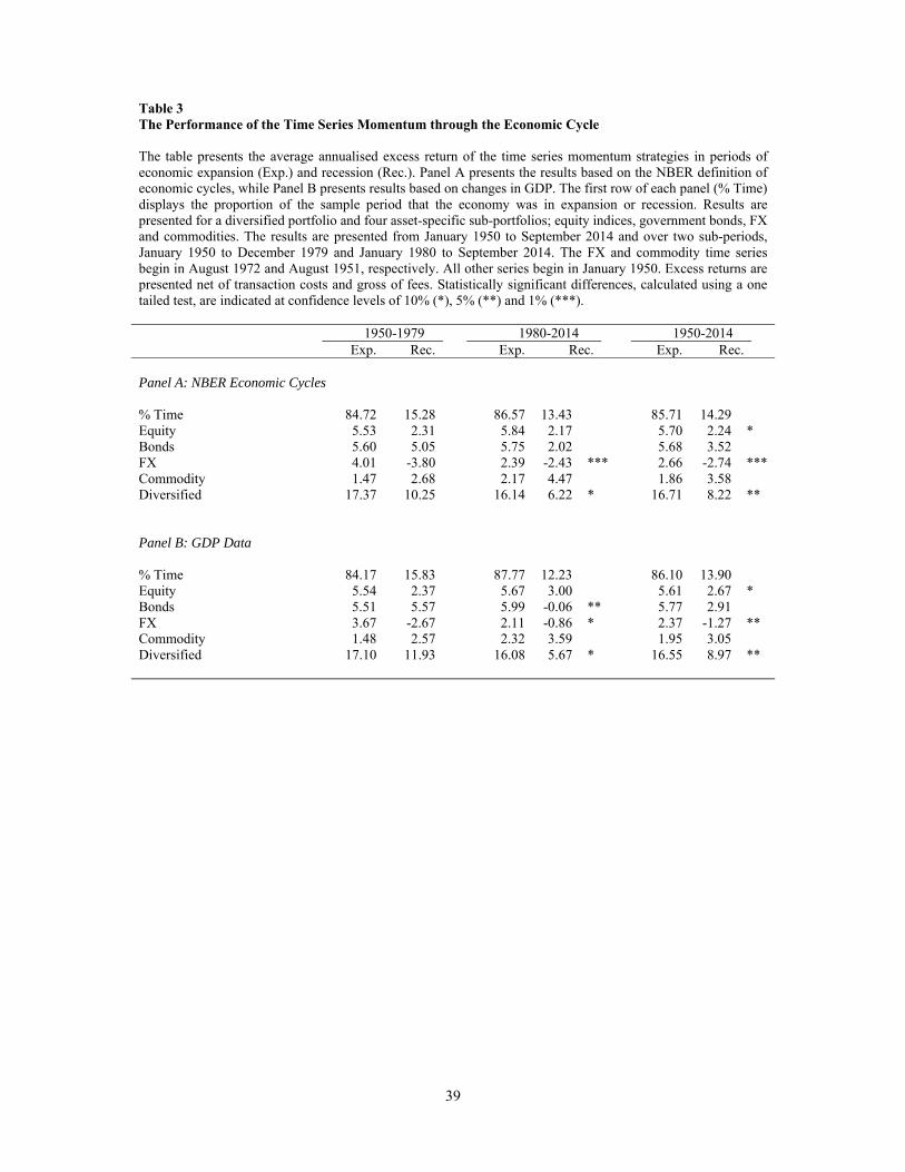
with a recession.14 The results are displayed in Table 3.
[Insert Table 3 here]
Using either definition, the economy expands in approximately 85% of months and
contracts in 15% of months, a pattern repeated in both sub-periods. Irrespective of the
14 There is overlap between four of the ten NBER recessions analysed here and four of the five post-1950 global financial crises twenty four month periods examined in Hutchinson and O'Brien (2014) , though the NBER recessions are much shorter (average peak to trough length of 11.1 months).
13
definition the results of the analysis are consistent. The diversified, equity, bond and FX
portfolios generate higher returns in periods of expansion than recession. This is seen over
both the full sample and, in general, across the sub-periods.15 Over the full period the average
performance in expansions exceeds that in recessions by a statistically significant 8.5%
(NBER) and 7.6% (GDP).
Consistent with the results of Hutchinson and O’Brien (2014) the commodity
portfolio provides an exception to this pattern, performing better in recessions than
expansions, returning 3.58% in recessions against 1.86% in expansions (NBER definition).
This result highlights the diversification benefits of commodities in a time series momentum
portfolio.
Spread states
In order to further explore the relationship between economic conditions and the
performance of times series momentum we define economic conditions using two key
interest rate spreads. These proxy for short term (term spread) and long term (default spread)
peaks and troughs in the business cycles (Fama and French (1989)). The term spread is
defined as the difference between the 10 year and three month US treasury rate and the
default spread is the difference between the BAA and AAA rated US corporate bonds.
In the following analyses, a month is defined as High (Low) if the value of the
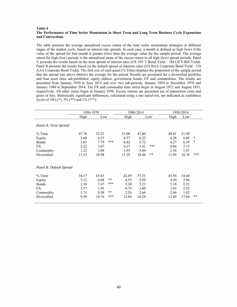
variable in that month is higher (lower) than the mean for the sample period.16 The results are
displayed in Table 4.
[Insert Table 4 here]
15 In the first sub-period bond time series momentum returns are marginally greater in expansion periods using the NBER measure (5.60% compared to 5.05%), while they are marginally smaller using the GDP measure (5.51% against 5.57%). 16 The definition of months as high (low) in a sub period is defined relative to the mean value for that sub-period. This can lead to months being defined differently depending on the sample period mean.
14
The diversified portfolio performs better in periods where the term spread is low, at
business cycle peaks. It generates a return of 18.76% in the low term spread state compared
to 11.95% in the high state over the full period, a statistically significant difference of 6.8%.
It also performs better in the low state relative to the high state in both sub-periods. In general
the sub-portfolios also outperform in the low term spread state over the full period and both
sub-periods.17
The pattern is repeated when looking at the default spread, where the time series
momentum portfolios perform better in the low state, a proxy for expansions. Here the
diversified portfolio generates a statistically significantly different return of 17.84% in the
low spread state compared to 12.69% in the high state. Again, looking at the sub-portfolios
and sub-periods, all typically perform better in the low default spread state compared to the
high state.
5.0 Economic factor model analysis
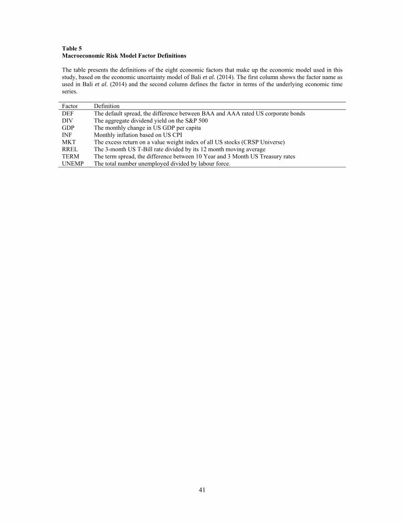
The Bali et al. (2014) model has eight economic and financial factors which have
been shown to be particularly important for hedge funds. The factors are commonly used in
literature, examples of which can be found in the models of Chen et al. (1986), Fama and
French (1989) and Chordia and Shivakumar (2002).
The term structure (TERM) and default spread (DEF) are included in all three of the
models listed above. Fama and French (1988) show that the variables track the long term and
short term business cycles, respectively. The dividend yield (DIV) is associated with mean
reversion in the stock markets and can also be interpreted as a proxy for time variation in risk
premia (Chordia and Shivakumar (2002)). The change in GDP and the level of
unemployment (UNEMP) capture current economic conditions. Short term interest rates 17 There is one exception; in the 1950 to 1979 sub-sample period the equity portfolio marginally outperforms in the high term spread state.
15
(RREL) capture both expectations about future economic activity (Chordia and Shivakumar
(2002)) and predict future equity market returns. Market returns (MKT) reflect changes in
expectations of future growth.18
The definitions of the eight factors are given in Table 5.
[Insert Table 5 here]
The ability of the economic model to explain time series momentum returns is tested
using two different sets of assumptions. First, that the relationship between the factors and the
methodologies is constant through time, a linear factor (unconditional) model and then
allowing the relationship to vary through time (conditional model).
5.1 Linear factor model
The linear factor model specifies economic factors as explanatory variables in the
regression model
r β ∑ β EF ε (6)
Where EF is the value of economic factor n at time t. N is the total number of
explanatory variables (economic factors) and r is the return of the time series momentum
portfolio in time period t. The factor model is estimated for the full sample period and the two
sub-periods. The ability of the factors to explain the returns of a time series momentum
strategy is assessed based upon the magnitude and statistical significance of the respective
regression co-efficient. A statistically significant regression coefficient is evidence of a
relationship between the returns of time series momentum and economic conditions.
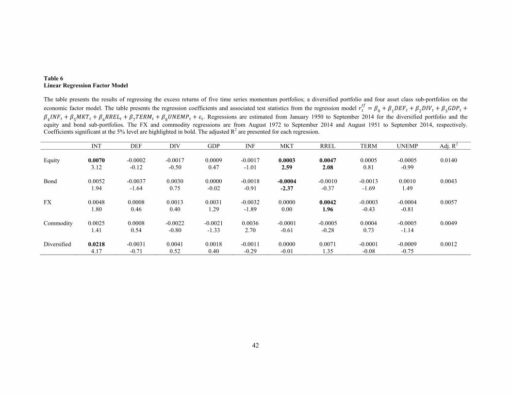
The results for the linear factor model are presented in Table 6. 18 To correct for long term trends in our extended sample period, the dividend yield factor (DIV) is measured relative to the lagged five year moving average and the short term rate (RREL) is calculated as a quotient rather than a difference.
16
[Insert Table 6 here]
The table lists the factors and their corresponding t-statistics. Consistent with
Moskowitz et al. (2012), the linear model provides little explanatory power for time series
momentum at the portfolio or sub-portfolio level. Only four, of forty, coefficients are
statistically significant. The market return factor (MKT) is significant for Equity and Bond
portfolios and the short term rate (RREL) is significant for both the Equity and FX portfolios.
At the diversified portfolio level, there is no statistically significant explanatory factor. The
inability of a linear economic factor model to explain returns is reflected in the low values
reported for the adjusted R2 measure, which range from 0.12% to 1.40%.
5.2 Conditional factor model
The explanatory power of a conditional model can vary considerably from the
unconditional (linear) specification (Griffin et al. (2003)), consequently we define a
conditional test based on the methodology used in Chordia and Shivakumar (2002) and
Griffin et al. (2003).
To allow for a time varying relationship between the time series momentum excess
returns and the macroeconomic factors, at each month, we estimate, using the current month
and prior 59 months, equation (7).19
r β ∑ β EF ε (7)
Where EF is the value of economic factor n at time t. N is the total number of
explanatory variables (economic factors) and r is the return of the time series momentum
portfolio in time period t. We utilise a minimum of 60 months of data for our regressions and
19 We use a 60 month estimation period for the conditional model and portfolio study consistent with the cross sectional momentum literature (Chordia and Shivakumar (2002)). In unreported analyses, we alternately use a 36 and 84 month estimation period. The results are very similar to those reported.
17
the t-statistics are based on Newey-West serial correlation consistent standard errors, since
the rolling regressions are subject to autocorrelation in the estimates. If the economic factors
fail to fully explain the returns from time series momentum, the intercept of the regression
model will be positive and statistically significant.
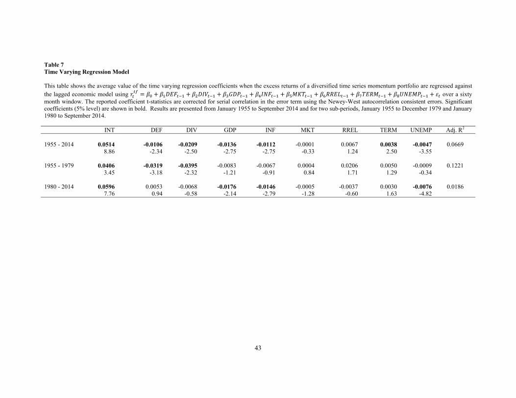
In Table 7 we report the results of estimating a conditional model which allows for
time variation - the average coefficients from the rolling five year lagged regressions and
their statistical significance. Unlike the unconditional model, six of the eight macroeconomic
factors have statistically significant coefficients for the full sample. This evidence highlights
that the conditional implementation of the model has some explanatory power for time series
momentum returns.
[Insert Table 7 here]
However, it is also noteworthy that the intercept for the model is positive and
statistically significant in all three of the periods, consistent with time series momentum
returns not being fully explained by the economic model. Later we investigate what portion
of returns is attributable to macroeconomic risk exposure.
5.3 Time series momentum and traditional asset classes
To highlight the time varying nature of the risk exposure of the time series momentum
portfolios we show the return series of time series momentum, the relationship (beta) between
these series and equity and bond markets in Figure 2. The excess total return of the S&P 500
Index is used to represent the equity market, while the excess total return of the 10 Year US
Treasury Bond at constant maturity is used as a proxy for the bond market. Each graph
displays three data series; the mean monthly return of the market factor over the prior sixty
months, the mean monthly return of the time series momentum portfolio over the same
18
period, and the beta of the time series momentum portfolio estimated relative to the relevant
financial market, again over the prior sixty months.
[Insert Figure 2 here]
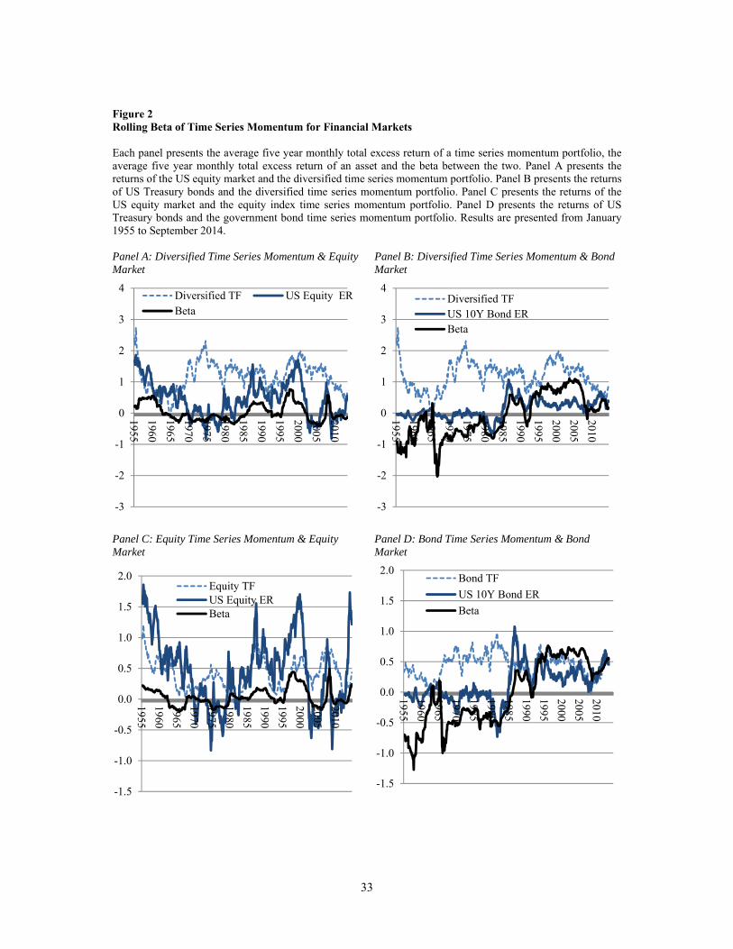
Panel A shows the relationship between the diversified time series momentum
portfolio and the equity market. Over the full period, the five year returns of the equity
market are generally positive, and during this period the beta of the diversified portfolio is on
average positive, reaching a maximum value of 0.75. The periods of negative beta, running
approximately from 1970 to 1985 correspond to a poor period of performance for the equity
market, where the return is lower than average and negative for a five year period around
1975. Two periods of negative beta occur after 2000 and coincide with falling equity markets
in the periods following the collapse of the dotcom bubble and the failure of Lehman
Brothers. Examining the relationship between the equity time series momentum portfolio and
the equity market (Panel C) produces a very similar pattern; positive betas when equity
markets are rising and negative betas when they are falling.
A similar analysis for the bond market is reported in Panel B and D. The excess return
of the bond market can be divided into two distinct periods split by the peak of the great
inflation in 1982. In the first period, bonds have a flat to small negative excess total return.
Since then the excess returns of bonds have been consistently positive. Strikingly, the returns
of the time series momentum portfolios are positive across all bond market conditions. In the
early period, both the global and bond time series momentum portfolios have a significant
negative relationship (beta) with the bond market excess return. In the later sub-period when
bond returns are positive the portfolio beta is also positive. This provides evidence that time
series momentum is profitable in rising and falling interest rate environments.
6.0 Momentum and asset-specific returns
19
Returns to the cross sectional momentum strategy have been shown to be primarily
due to the component of individual equity returns explained by macroeconomic factors
(Chordia and Shivakumar (2002)). This is important as it shows that the returns to cross
sectional momentum are in large part due to exposure to macroeconomic risk. In order to
examine if this is also the case for time series momentum, we create two alternative time
series momentum portfolios based on the decomposition of asset returns into a
macroeconomic factor-related component (factor-related returns) and an idiosyncratic
component specific to the individual asset (asset-specific returns).
This decomposition produces two return series, factor-related and asset-specific, for
each instrument. Each series is used as the basis for the creation of a set of time series
momentum portfolios using the methodology described above.
The factor-related time series momentum strategy generates a trading signal for each
futures contract from its factor-related return, whereas the asset-specific time series
momentum portfolio is built using a signal generated from the component of each futures
contract return not explained by the factor model.
The first step in this process is to decompose the returns of each futures contract into
factor-related and asset-specific components. We define the regression model to explain the
factor-related price movement following Grundy and Martin (2001) and Chordia and
Shivakumar (2002). The model is estimated for each futures contract for each month, using
the current month and prior 59 months’ returns. Estimating the model using a rolling
regression allows us to identify the time varying factor-related return.
r β , ∑ β , ∆F ε (8)
20
Where r is the excess return of futures contract i in time period t, ∆F is the change
in factor n in time period t and ε is the error term. The model has N factors. The regression
coefficients β , and β , are the coefficients for the model estimated over the period t-59 to t,
where β , is the regression intercept and β , is the regression coefficient for factor n.
The factor-related return of each instrument at time t is then estimated as
β , ∑ , ∆ (9)
Where is the factor-related return of instrument i, at time t. The corresponding
asset-specific return, , is then calculated as the difference between the excess return and
factor-related return at time t.
(10)
We then form two alternative time series momentum portfolios using, alternately,
factor-related returns and asset-specific returns (rather than raw excess returns) to generate
the trading signal.
Under this construction, if time series momentum returns are entirely due to exposure
to macroeconomic risk then only the portfolios formed on factor-related returns should yield
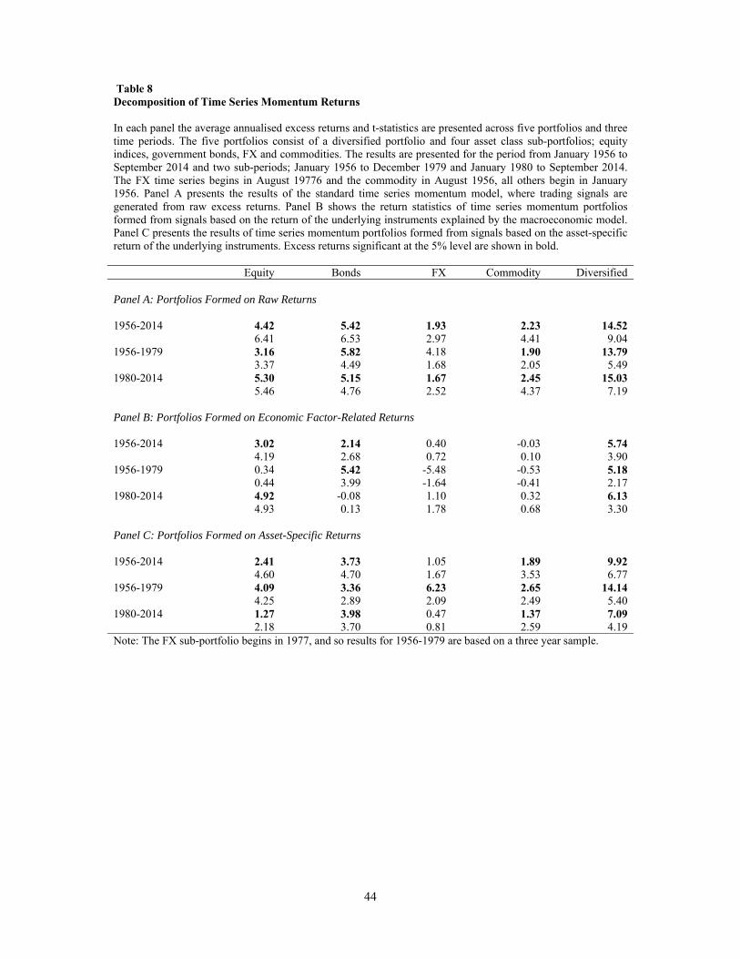
positive payoffs. The cumulative returns are reported in Figure 3 and the summary statistics
of the different portfolios are displayed in Table 8.20
[Insert Figure 3 here]
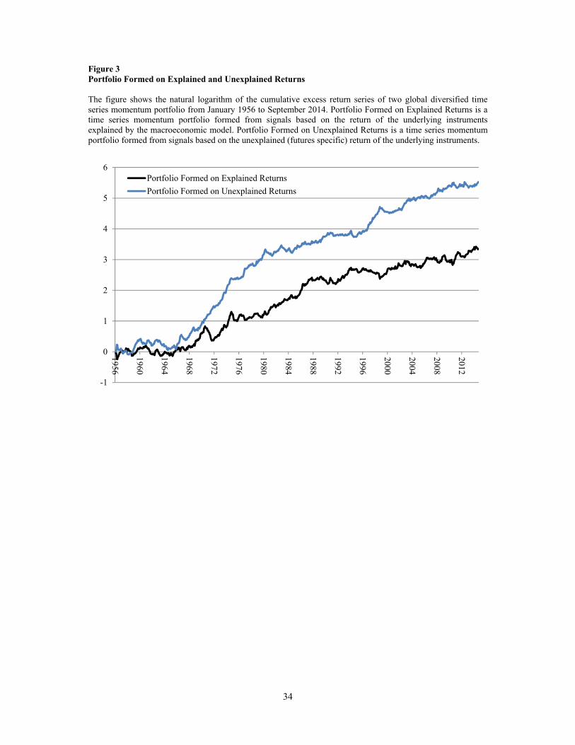
Looking first at the diversified portfolio, it can be seen that statistically significant
excess returns are generated by both sets of portfolios, factor-related (Panel B) and asset-
20 Results are reported from January 1956 as we use a 60 month period to decompose futures returns and a further 12 month formation period for the initial time series momentum signals.

21
specific (Panel C) futures returns over the full sample period and both sub-periods.21 Over the
full period, the portfolio formed on asset-specific returns generates an annual excess return of
9.92% compared to 5.74% for the portfolio formed on factor-related returns. Looking at the
results over the two sub-periods, the portfolio formed on macroeconomic factor-related
returns is consistent, with payoffs of 5.18% and 6.13% respectively. The asset-specific return
portfolio shows a different pattern, with an excess return of 14.14% in the earlier period and
7.09% since 1980.
[Insert Table 8 here]
For individual markets, all the sub-portfolios have positive returns for the asset-
specific return portfolios and in all but two cases these are statistically significant. The factor-
related portfolio returns are quite different. While the equity and bond portfolios produce
statistically positive returns over the full period, the FX return is only marginally positive and
the commodity return is close to zero. Results are more mixed over the sub-periods where,
while the majority of the returns are positive, only two are statistically significant.
7.0 Economic uncertainty
Recent evidence on time series momentum has highlighted that the performance of
the strategy tends to be below average for an extended period following financial crises
(Hutchinson and O'Brien (2014)). Separately Bali et al. (2014) present evidence that
economic uncertainty plays a role in explaining the cross sectional deviation in the
performance of hedge funds. In order to identify if macroeconomic uncertainty is the
transmission mechanism linking macroeconomic factors and the results of Hutchinson and
O'Brien (2014) we specify a model of economic uncertainty, based on Bali et al. (2014),
21 The signal generating process of the portfolios is quite different reflected in a full sample correlation coefficient of -0.06 for the diversified portfolios formed on factor and idiosyncratic returns.
22
where the time varying conditional volatility of a set of eight economic variables is used as a
proxy for economic uncertainty.
Bali et al. (2014) define economic uncertainty as being a function of the time varying
conditional volatility of the eight risk factors. The time varying conditional volatility is
estimated using a vector auto regressive process to model the economic variables and a
GARCH model to capture the asymmetric response of volatility to change in the economy.
The auto regressive model is given as:
(11)
Where is an 8x1 matrix of the values of the eight variables at time t. is an
8x1 matrix of regression constants and is an 8x8 matrix of regression coefficients. is
the matrix of regression errors at time t. After regressing the model over the time period
January 1950 to September 2014, the expected volatility of each factor is estimated using a
multivariate asymmetric GARCH model, specifically the Threshold-GARCH (TGARCH)
model of Glosten et al. (1993). The asymmetry allows different responses to positive and
negative shocks to be modelled. The TGARCH model is:
, ≡ , , (12)
, 1 , 0, 0
Where , is the expected value of the square of the error term of variable i, at
time t. This is the conditional volatility , , of the instrument. is the coefficient n of
variable i. , is a dummy variable set to one for , 0 or zero otherwise. A positive value
for indicates negative shocks cause higher volatility than positive shocks.
23
The final stage of the process combines the volatilities of the eight factors to generate
an index of economic uncertainty. The volatilities of the factors are both persistent and cross
correlated, allowing the use of principle component analysis. Following Bali et al. (2014) we
use the first principle component to generate a linear function of the eight individual time
series.
Our methodology differs from Bali et al. (2014) in two ways. Bali et al. (2014) use a
recursive estimation procedure, whereas we use a single estimation for the full time period,
which induces a look-ahead bias. The advantage of our approach is that it allows us to begin
our analysis in 1950, maximising the sample of available economic data.22 While Bali et al.
(2014) estimate all parameters simultaneously, we estimate the economic model separately
from the T-GARCH volatility model.
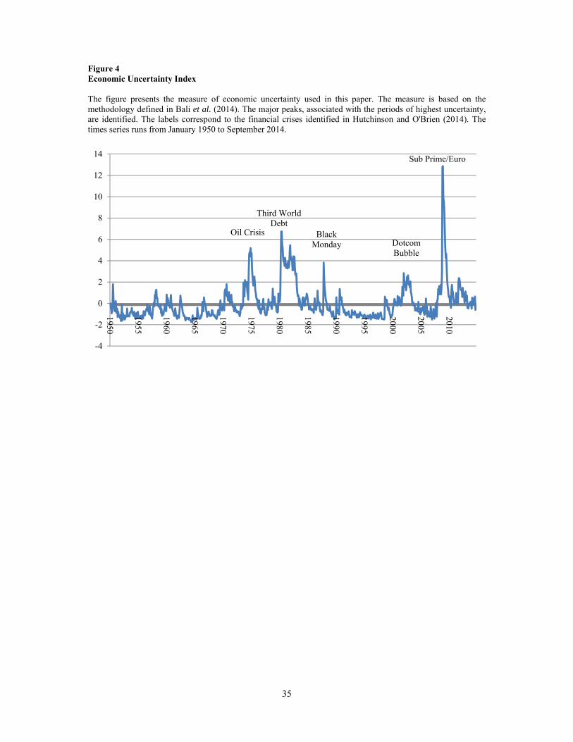
The economic uncertainty index based on Bali et al. (2014) is reported in Figure 4.
The measure varies through time, but peak economic uncertainty measured by the model
closely corresponds to the financial crises identified in Hutchinson and O'Brien (2014).
[Insert Figure 4 here]
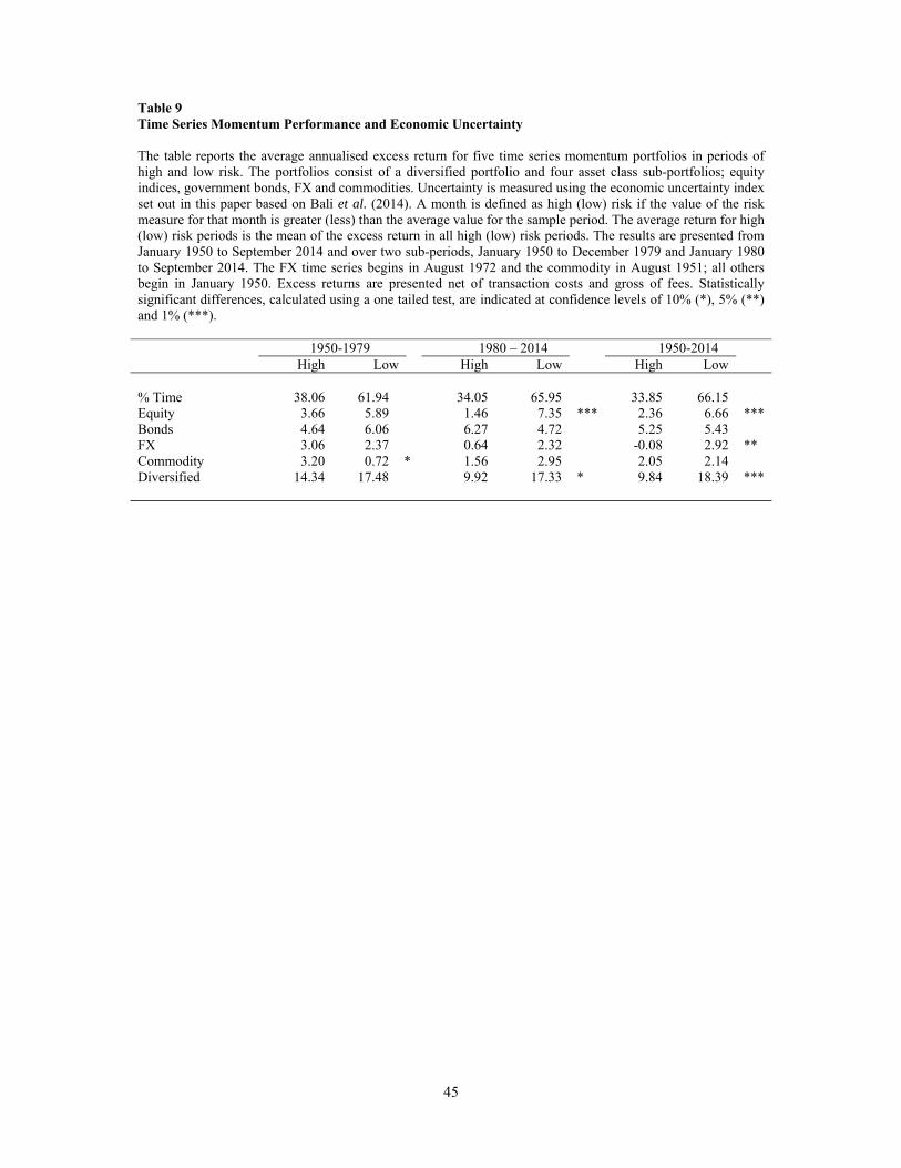
To see the impact of economic uncertainty on the performance of time series
momentum, we compare the performance in periods of high and low uncertainty over the full
period and each of the sub-periods. The markets are defined as high or low uncertainty by
comparing the level of economic uncertainty with its mean for the period.23 24 The results are
shown in Table 9.
22 The recursive estimation approach requires an extended window of data, prior to the sample period (Bali et al. (2014) use 23 years). As our economic data set begins in 1950, incorporating a similar formation period eliminates much of the first sub-sample period. 23 As the mean uncertainty is a function of the sub-period, individual months can be assigned to different states depending on the mean of the period under investigation. 24 Results are very similar when the analysis is based on the median of the series.
24
[Insert Table 9 here]
The diversified portfolio exhibits better performance in periods of below average
uncertainty for both the full sample period (18.39% against 9.84%) and both sub-periods,
(17.48% compared with 14.34% in the earlier period and 17.33% compared with 9.92% in
the later period). This pattern is evident in the equity and currency markets, over both the full
period and both sub-periods; although it should be noted the sample size for currencies is
small in the earlier period, running from 1972 to 1979.
The results for government bonds and commodities are less consistent. The
performance of the bond portfolio over the full period is marginally better when economic
uncertainty is reduced, while it performs better in low uncertainty conditions in the earlier
period and high uncertainty conditions in the later sub-period. The commodity portfolio again
shows a different pattern, with similar performance under high and low uncertainty over the
full periods and performing better in high uncertainty conditions in the first sub-period.
In order to further investigate the relationship between the returns and economic
uncertainty a series of regressions were carried out based on the model
(13)
Where is the return of the diversified time series momentum portfolio at time t,
and is the value of the economic uncertainty index at time t - l. The variable l is the
measure of the lag or lead of the uncertainty index relative to the return series. The test
statistics of the regression coefficients for a range of values of l (-18 to 18) is displayed in
Figure 5.
[Insert Figure 5 here]
25
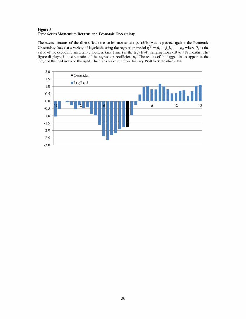
Figure 5 shows a statistically significant negative relationship between the returns to
time series momentum and the uncertainty index in the contemporaneous month and for lags
of up to six months. Following periods when economic uncertainty is low (high) the returns
of the time series momentum strategy are higher (lower) than average. Given the association
of economic uncertainty and periods following financial crises, this helps explain previous
findings that time series momentum returns are below average in the period after financial
crises (Hutchinson and O'Brien (2014)).
8. Conclusions
This article was motivated by two observations. First, CTAs have received large
inflows of capital following the 2008 financial crisis. Second, investors’ motivation for
allocating to CTAs is often due to an expectation of performance in equity bear markets,
without a consideration of performance in other market states, or the drivers of performance.
We have shown that the returns to time series momentum are connected to the business cycle.
Time series momentum earns positive returns in both expansions and recessions but the
returns are especially strong in expansions. Whether we measure the business cycle using
NBER data, GDP data or use interest rate spreads as proxies for short and long term
fluctuations, our results are consistent. Returns are statistically significantly higher by
between 5% and 8% in expansions. These findings dispel the notion that high returns to time
series momentum are specific to equity market states.
Taken together our results provide a degree of clarity on the return drivers of time
series momentum. Complementing Moskowitz et al. (2012) who document a behavioural
driver, we find that there is a role for rational price theories to explain a portion of time series
momentum profitability. We find that the returns are related to a set of macroeconomic
factors that have been shown in the literature to be important in explaining the returns of
26
traditional asset classes and hedge funds. Our results indicate that about 40 percent of the
returns of time series momentum are due to time varying exposure to these macroeconomic
variables, which are related to the business cycle. These findings are consistent with the
conclusions of Chordia and Shivakumar (2002) for cross sectional momentum, that a portion
of the profitability of momentum strategies represents compensation for bearing time varying
risk, consistent with rational asset pricing theories.
Finally, we note the interesting finding that the performance of time series momentum
improves when economic uncertainty is diminished. This result provides a link between the
finding of Hutchinson and O'Brien (2014), that time series momentum tends to perform less
well than average following periods of financial crisis, and changes in the business cycle.
Using a new methodology, we document that uncertainty is the transmission mechanism
linking changes in the macroeconomic variables and changes in the performance of time
series momentum following financial crisis.
27
Bali, T.G., Brown, S.J., Caglayan, M.O., 2014. Macroeconomic risk and hedge fund returns.
Journal of Financial Economics 114, 1-19
Baltas, A.-N., Kosowski, R., 2013. Momentum Strategies in Futures Markets and Trend-
following Funds. Paris December 2012 Finance Meeting EUROFIDAI-AFFI Paper
Chen, N.-F., Roll, R., Ross, S.A., 1986. Economic forces and the stock market. Journal of
Business, 383-403
Chordia, T., Shivakumar, L., 2002. Momentum, Business Cycle, and Time-varying Expected
Returns. Journal of Finance 57, 985-1019
Conrad, J., Kaul, G., 1998. An anatomy of trading strategies. Review of Financial Studies 11,
489-519
Erb, C.B., Harvey, C.R., 2006. The strategic and tactical value of commodity futures.
Financial Analysts Journal 62, 69-97
Fama, E.F., French, K.R., 1988. Dividend yields and expected stock returns. Journal of
Financial Economics 22, 3-25
Fama, E.F., French, K.R., 1989. Business Conditions and Expected Returns on Stocks and
Bonds. Journal of Financial Economics 25, 23-49
Fuertes, A.-M., Miffre, J., Rallis, G., 2010. Tactical allocation in commodity futures markets:
Combining momentum and term structure signals. Journal of Banking and Finance
34, 2530-2548
Glosten, L.R., Jagannathan, R., Runkle, D.E., 1993. On the Relation between the Expected
Value and the Volatility of the Nominal Excess Return on Stocks. Journal of Finance
48, 1779-1801
Goyal, A., Jegadeesh, N., 2015. Cross-Sectional and Time-Series Tests of Return
Predictability: What is the Difference? Available at SSRN 2610288
Griffin, J.M., Ji, X., Martin, J.S., 2003. Momentum Investing and Business Cycle Risk:
Evidence from Pole to Pole. Journal of Finance 58, 2515-2547
Grundy, B.D., Martin, J.S., 2001. Understanding the nature of the risks and the source of the
rewards to momentum investing. Review of Financial Studies 14, 29-78
Hurst, B., Ooi, Y.H., Pedersen, L.H., 2012. A Century of Evidence on Trend-Following
Investing. AQR Management, 1-11
Hutchinson, M.C., O'Brien, J.J., 2014. Is This Time Different? Trend Following and
Financial Crises. Journal of Alternative Investments 17, 82-102
Menkhoff, L., Sarno, L., Schmeling, M., Schrimpf, A., 2012. Currency momentum strategies.
Journal of Financial Economics 106, 660-684

28
Miffre, J., Rallis, G., 2007. Momentum strategies in commodity futures markets. Journal of
Banking and Finance 31, 1863-1886
Moskowitz, T.J., Ooi, Y.H., Pedersen, L.H., 2012. Time series momentum. Journal of
Financial Economics 104, 228-250
Okunev, J., White, D., 2003. Do momentum-based strategies still work in foreign currency
markets? Journal of Financial and Quantitative Analysis 38, 425-448
29
Appendix A: Data Sources
A.1 Equity indices
The universe of equity indices has twenty components. Fourteen of these consist of
data from developed markets, with future prices available from Datastream starting at various
dates from January 1980 and derived forward prices generated from data provided by Global
Financial Data prior to that. In each case Global Financial Data provides a total return index,
which allows the yield to be calculated. This group consists of Australia (SPI200), Canada
(TSX 60), Netherlands (AEX), France (CAC 40), Germany (DAX), Hong Kong (Hang
Seng), Korea (KOSPI 200), Japan (Nikkei 225), United States (S&P 500), United Kingdom
(FTSE 100), Spain (IBES 35), Italy (MIB), Sweden (OMX 30) and Switzerland (SMI).
The six additional indices are the three mid cap indices (Germany, Switzerland and
United States) and three alternative indices for the US (Dow Jones, Russell 2000 and
NASDAQ 100). We only include exchange traded future contract data for these indices.
A.2 Bond indices
A total of thirteen government bond indices from six countries are used. Australia (10
and 3 year), Canada (10 year), United States (2, 5, 10 and 30 year), Germany (2 ,5, 10 and 30
year), Japan (10 year) and United Kingdom (10 year). Exchange data for these is from
Datastream, starting on a variety of dates from January 1980. Data for eight of these is
extended backwards using total return indices and short term yields from Global Financial
Data.
A.3 Currencies
The universe of currency forwards consists of ten currencies. Forwards are created for
all currency pairs from spot data and short term interest rates. The spot rates are sources from
30
Datastream/MSCI from 1980 and, prior to that, from Global Financial Data. Although data is
available back to 1920, currencies are only considered for inclusion and statistics provided
from the end of the Bretton-Woods fixed rate system in 1971. The Euro and German Mark
are spliced into one time series. The currencies included are Australia, Canada, Euro
(Germany), Norway, New Zealand, Sweden, Switzerland, United Kingdom and United
States.
A.4 Commodities
Twenty one commodities are included; Copper, Gold and Silver (COMEX), Light
Crude Oil, Natural Gas, NY Heating Oil, Palladium, Platinum and RBOB Gasoline
(NYMEX), Cocoa, Coffee, Cotton, Gas Oil and Sugar (ICE), Corn, Soya Bean Oil, Soya
Bean Meal, Soya Beans and Wheat (CME) and Lean Hogs and Live Cattle (CBOT). The
commodity data is entirely based on prices of exchange traded futures. As cost of carry data
is unavailable it is not possible to accurately estimate forward prices prior to the availability
of exchange traded futures. The commodity data from 1980 was sourced from DataStream
while the earlier data was sourced from Commodity Systems Inc. (CSI). The Copper contract
consists of a combination of the medium grade copper contract traded until l988 and the high
grade copper contract traded since then, sourced from CSI and DataStream respectively.
A.5 Risk free rates
Short term interest rates are sourced from Global Financial Data due to more extensive
coverage. The one month interbank rate (LIBOR or equivalent) is the preferred rate. When
this is not available, the closest available interbank rate was used, and finally the central bank
base rate.
A.6 Economic factor model
31
Table 10 shows the data sources used for the primary data used to define the
economic factor model. All data is available from January 1950, with the exception of the
yield of the 10 Year US Treasury Bond (constant maturity), which becomes available from
1952. The first two years of this time series were back filled using the US 10 Year Treasury
Bond Yield from the same source.
[Insert Table 10 here]
32
Figure 1 Performance of the Diversified Time Series Momentum Portfolio The figure shows the natural logarithm of the cumulative excess return series of a diversified time series momentum portfolio from January 1950 to September 2014. Excess returns are presented net of transaction costs and gross of fees.
-2
0
2
4
6
8
10
1950
1955
1960
1965
1970
1975
1980
1985
1990
1995
2000
2005
2010
33
Figure 2 Rolling Beta of Time Series Momentum for Financial Markets Each panel presents the average five year monthly total excess return of a time series momentum portfolio, the average five year monthly total excess return of an asset and the beta between the two. Panel A presents the returns of the US equity market and the diversified time series momentum portfolio. Panel B presents the returns of US Treasury bonds and the diversified time series momentum portfolio. Panel C presents the returns of the US equity market and the equity index time series momentum portfolio. Panel D presents the returns of US Treasury bonds and the government bond time series momentum portfolio. Results are presented from January 1955 to September 2014. Panel A: Diversified Time Series Momentum & Equity Market
Panel B: Diversified Time Series Momentum & Bond Market
Panel C: Equity Time Series Momentum & Equity Market
Panel D: Bond Time Series Momentum & Bond Market
-3
-2
-1
0
1
2
3
4
1955
1960
1965
1970
1975
1980
1985
1990
1995
2000
2005
2010
Diversified TF US Equity ERBeta
-3
-2
-1
0
1
2
3
4
1955
1960
1965
1970
1975
1980
1985
1990
1995
2000
2005
2010
Diversified TFUS 10Y Bond ERBeta
-1.5
-1.0
-0.5
0.0
0.5
1.0
1.5
2.0
1955
1960
1965
1970
1975
1980
1985
1990
1995
2000
2005
2010
Equity TFUS Equity ERBeta
-1.5
-1.0
-0.5
0.0
0.5
1.0
1.5
2.0
1955
1960
1965
1970
1975
1980
1985
1990
1995
2000
2005
2010
Bond TF
US 10Y Bond ER
Beta
34
Figure 3 Portfolio Formed on Explained and Unexplained Returns The figure shows the natural logarithm of the cumulative excess return series of two global diversified time series momentum portfolio from January 1956 to September 2014. Portfolio Formed on Explained Returns is a time series momentum portfolio formed from signals based on the return of the underlying instruments explained by the macroeconomic model. Portfolio Formed on Unexplained Returns is a time series momentum portfolio formed from signals based on the unexplained (futures specific) return of the underlying instruments.
-1
0
1
2
3
4
5
6
1956
1960
1964
1968
1972
1976
1980
1984
1988
1992
1996
2000
2004
2008
2012
Portfolio Formed on Explained Returns
Portfolio Formed on Unexplained Returns
35
Figure 4 Economic Uncertainty Index The figure presents the measure of economic uncertainty used in this paper. The measure is based on the methodology defined in Bali et al. (2014). The major peaks, associated with the periods of highest uncertainty, are identified. The labels correspond to the financial crises identified in Hutchinson and O'Brien (2014). The times series runs from January 1950 to September 2014.
-4
-2
0
2
4
6
8
10
12
14
1950
1955
1960
1965
1970
1975
1980
1985
1990
1995
2000
2005
2010
BlackMonday
Oil Crisis
Third World Debt
Sub Prime/Euro
Dotcom Bubble
36
Figure 5 Time Series Momentum Returns and Economic Uncertainty The excess returns of the diversified time series momentum portfolio was regressed against the Economic Uncertainty Index at a variety of lags/leads using the regression model , where is the value of the economic uncertainty index at time t and l is the lag (lead), ranging from -18 to +18 months. The figure displays the test statistics of the regression coefficient . The results of the lagged index appear to the left, and the lead index to the right. The times series run from January 1950 to September 2014.
-3.0
-2.5
-2.0
-1.5
-1.0
-0.5
0.0
0.5
1.0
1.5
2.0
-18 -12 -6 0 6 12 18
Coincident
Lag/Lead
37
Table 1 Future Contracts The table provides a list of the underlying futures contracts used to create the time series momentum portfolios used in this study. Each future is listed with its average annual excess return, volatility and the date the return series becomes available. The futures are divided into four classes; Commodities, Government Bonds, Equity Indices and currencies. All data series end in September 2014. Start
Date Annual Return
Annual Vol.
Start Date
Annual Return
Annual Vol.
Commodity Futures Equity Index Futures COCOA Jan-66 -0.48 28.56 SPI 200 - Australia Jan-50 3.78 17.01 COFFEE Sep-72 -1.47 37.87 S&P TSX60- Canada Jan-70 3.19 16.42 COPPER Jan-66 4.23 27.51 Dow Jones-US Oct-77 4.12 15.28 CORN Aug-50 -3.24 22.26 NASDAQ 100 - US Apr-96 8.18 27.29 COTTON Apr-67 -0.83 25.39 AEX - Netherlands Jan-70 5.02 18.91 GAS OIL Sep-03 9.78 28.87 CAC 40 France Jan-70 3.36 20.26 GOLD Feb-75 3.97 19.97 DAX - Germany Jan-50 5.82 18.50 LEAN HOGS Mar-66 2.94 26.05 MDAX -Germany Mar-05 11.14 21.36 LIGHT CRUDE OIL Mar-83 6.14 33.96 HANG SENG - Hong Kong Jan-70 10.53 33.29 LIVE CATTLE Dec-64 4.31 16.91 S&P Midcap- US Feb-92 8.19 16.78 NATURAL GAS Apr-90 -10.76 56.64 NIKKIE 225 - Japan Jan-50 6.08 20.30 NY HEATING OIL Jan-80 6.12 31.97 S&P 500 – US Jan-50 5.48 14.52 PALLADIUM Feb-77 5.75 35.08 KOSPI 200 - Korea Jan-65 8.86 27.38 PLATINUM Feb-64 2.99 26.91 FTSE 100- UK Jan-50 5.05 17.90 RBOB GASOLINE Oct-05 6.20 32.28 IBEX 35 - Spain Jan-70 1.68 20.85 SILVER Jul-73 -0.51 31.00 MIB – Italy Jan-50 2.11 21.95 SOYABEAN MEAL Sep-51 3.57 28.69 Russell 2000 - US Aug-07 6.09 21.91 SOYABEAN OIL Aug-50 6.84 27.79 OMXS 30 - Sweden Jan-70 6.77 21.93 SOYABEANS Aug-50 3.31 24.02 SMI - Switzerland Jan-70 5.39 16.45SUGAR Jan-66 -2.99 40.52 SMI Midcap - Switzerland Sep-05 6.17 17.47 WHEAT Aug-50 -4.09 23.14 Bond Futures Currency Forwards Australia-10Y Jan-50 0.50 6.73 AUD/USD Aug-71 -1.69 11.51Australia-3Y May-88 4.03 9.47 CAD/USD Aug-71 -0.39 6.54 Canada-10Y Jan-50 1.29 6.22 CHF/USD Aug-71 -0.80 12.23 US-5Y Jan-50 0.82 4.98 EUR/USD* Aug-71 0.11 10.91US-2Y Jun-90 1.62 1.68 GBP/USD Aug-71 -0.77 10.15 US-10Y Jan-50 1.21 6.75 JPY/USD Aug-71 -0.14 11.18 US-30Y Jan-50 0.78 9.77 NOK/USD Aug-71 -1.36 10.58Germany-5Y Oct-91 2.97 3.22 NZD/USD Aug-71 -1.97 12.41 Germany-30Y Sep-05 5.34 11.88 SEK/USD Aug-71 0.05 11.03 Germany-2Y Mar-97 0.92 1.32 Germany-10Y Jan-50 2.33 5.05 Japan-10Y Jan-50 2.67 6.15 UK-10Y Jan-50 1.21 8.27 * DEM/USD prior to the introduction of the Euro in Jan 1999
38
Table 2 Performance of Time Series Momentum Portfolios The table reports the average annualised excess return and volatility of five time series momentum portfolios, comprising of a diversified portfolio and four asset class sub-portfolios; equity indices (Equity), government bonds (Bonds), currencies (FX) and commodities (Commodity). The results are presented from January 1950 to September 2014 and over two sub-periods, January 1950 to December 1979 and January 1980 to September 2014. The FX and Commodity time series begin in August 1972 and August 1951, respectively. All other series begin in January 1950. Excess returns are presented net of transaction costs and gross of fees. Diversified Equity Bonds FX Commodity 1950-2014 Return (%) 15.75 5.18 5.29 1.81 2.04 Vol. (%) 12.55 5.41 6.39 4.45 4.17 1950-1979 Return (%) 16.60 5.03 5.46 2.46 1.55 Vol. (%) 13.01 4.97 6.26 5.91 5.00 1980-2014 Return 15.03 5.30 5.15 1.67 2.45 Vol. (%) 12.14 5.77 6.50 4.08 3.34
39
Table 3 The Performance of the Time Series Momentum through the Economic Cycle The table presents the average annualised excess return of the time series momentum strategies in periods of economic expansion (Exp.) and recession (Rec.). Panel A presents the results based on the NBER definition of economic cycles, while Panel B presents results based on changes in GDP. The first row of each panel (% Time) displays the proportion of the sample period that the economy was in expansion or recession. Results are presented for a diversified portfolio and four asset-specific sub-portfolios; equity indices, government bonds, FX and commodities. The results are presented from January 1950 to September 2014 and over two sub-periods, January 1950 to December 1979 and January 1980 to September 2014. The FX and commodity time series begin in August 1972 and August 1951, respectively. All other series begin in January 1950. Excess returns are presented net of transaction costs and gross of fees. Statistically significant differences, calculated using a one tailed test, are indicated at confidence levels of 10% (*), 5% (**) and 1% (***). 1950-1979 1980-2014 1950-2014 Exp. Rec. Exp. Rec. Exp. Rec. Panel A: NBER Economic Cycles % Time 84.72 15.28 86.57 13.43 85.71 14.29 Equity 5.53 2.31 5.84 2.17 5.70 2.24 * Bonds 5.60 5.05 5.75 2.02 5.68 3.52 FX 4.01 -3.80 2.39 -2.43 *** 2.66 -2.74 *** Commodity 1.47 2.68 2.17 4.47 1.86 3.58 Diversified 17.37 10.25 16.14 6.22 * 16.71 8.22 ** Panel B: GDP Data % Time 84.17 15.83 87.77 12.23 86.10 13.90 Equity 5.54 2.37 5.67 3.00 5.61 2.67 * Bonds 5.51 5.57 5.99 -0.06 ** 5.77 2.91 FX 3.67 -2.67 2.11 -0.86 * 2.37 -1.27 **Commodity 1.48 2.57 2.32 3.59 1.95 3.05 Diversified 17.10 11.93 16.08 5.67 * 16.55 8.97 **
40
Table 4 The Performance of Time Series Momentum in Short Term and Long Term Business Cycle Expansions and Contractions The table presents the average annualised excess return of the time series momentum strategies at different stages of the market cycle, based on interest rate spreads. In each case, a month is defined as high (low) if the value of the spread for that month is greater (less) than the average value for the sample period. The average return for high (low) periods is the annualized mean of the excess return in all high (low) spread periods. Panel A presents the results based on the term spread of interest rates (US 10Y T-Bond Yield – 3M US T-Bill Yield). Panel B presents the results based on the default spread of interests rates (US BAA Corporate Bond Yield – US AAA Corporate Bond Yield). The first row of each panel (% Time) displays the proportion of the sample period that the spread was above (below) the average for the period. Results are presented for a diversified portfolio and four asset class sub-portfolios; equity indices, government bonds, FX and commodities. The results are presented from January 1950 to June 2013 and over two sub-periods, January 1950 to December 1979 and January 1980 to September 2014. The FX and commodity time series begin in August 1972 and August 1951, respectively. All other series begin in January 1950. Excess returns are presented net of transaction costs and gross of fees. Statistically significant differences, calculated using a one tailed test, are indicated at confidence levels of 10% (*), 5% (**) and 1% (***). 1950-1979 1980-2014 1950-2014 High Low High Low High Low Panel A: Term Spread % Time 47.78 52.22 53.00 47.00 48.01 51.99 Equity 5.60 4.53 4.57 6.22 4.28 6.05 * Bonds 3.03 7.79 *** 4.82 5.72 4.27 6.39 * FX 2.22 3.07 0.27 3.41 *** 0.86 3.15 Commodity 1.22 2.09 1.93 3.09 2.36 1.87 Diversified 13.33 18.98 11.59 18.44 ** 11.95 18.76 *** Panel B: Default Spread
% Time 34.17 65.83 42.69 57.31 45.56 54.44 Equity 3.12 6.04 ** 4.53 5.95 4.30 5.96 Bonds 1.36 7.67 *** 5.30 5.21 5.18 5.53 FX 3.57 1.91 0.75 2.49 1.03 2.55 Commodity 3.71 0.58 ** 2.26 2.64 2.46 1.82 Diversified 9.59 19.76 *** 12.84 16.28 12.69 17.84 **
41
Table 5 Macroeconomic Risk Model Factor Definitions The table presents the definitions of the eight economic factors that make up the economic model used in this study, based on the economic uncertainty model of Bali et al. (2014). The first column shows the factor name as used in Bali et al. (2014) and the second column defines the factor in terms of the underlying economic time series. Factor Definition DEF The default spread, the difference between BAA and AAA rated US corporate bonds DIV The aggregate dividend yield on the S&P 500 GDP The monthly change in US GDP per capita INF Monthly inflation based on US CPI MKT The excess return on a value weight index of all US stocks (CRSP Universe) RREL The 3-month US T-Bill rate divided by its 12 month moving average TERM The term spread, the difference between 10 Year and 3 Month US Treasury rates UNEMP The total number unemployed divided by labour force.
42
Table 6 Linear Regression Factor Model The table presents the results of regressing the excess returns of five time series momentum portfolios; a diversified portfolio and four asset class sub-portfolios on the
economic factor model. The table presents the regression coefficients and associated test statistics from the regression model 0 1 2 3
4 5 6 7 8 . Regressions are estimated from January 1950 to September 2014 for the diversified portfolio and the equity and bond sub-portfolios. The FX and commodity regressions are from August 1972 to September 2014 and August 1951 to September 2014, respectively. Coefficients significant at the 5% level are highlighted in bold. The adjusted R2 are presented for each regression.
INT DEF DIV GDP INF MKT RREL TERM UNEMP Adj. R2
Equity 0.0070 -0.0002 -0.0017 0.0009 -0.0017 0.0003 0.0047 0.0005 -0.0005 0.0140 3.12 -0.12 -0.50 0.47 -1.01 2.59 2.08 0.81 -0.99 Bond 0.0052 -0.0037 0.0030 0.0000 -0.0018 -0.0004 -0.0010 -0.0013 0.0010 0.0043 1.94 -1.64 0.75 -0.02 -0.91 -2.37 -0.37 -1.69 1.49 FX 0.0048 0.0008 0.0013 0.0031 -0.0032 0.0000 0.0042 -0.0003 -0.0004 0.0057 1.80 0.46 0.40 1.29 -1.89 0.00 1.96 -0.43 -0.81 Commodity 0.0025 0.0008 -0.0022 -0.0021 0.0036 -0.0001 -0.0005 0.0004 -0.0005 0.0049 1.41 0.54 -0.80 -1.33 2.70 -0.61 -0.28 0.73 -1.14 Diversified 0.0218 -0.0031 0.0041 0.0018 -0.0011 0.0000 0.0071 -0.0001 -0.0009 0.0012 4.17 -0.71 0.52 0.40 -0.29 -0.01 1.35 -0.08 -0.75
43
Table 7 Time Varying Regression Model This table shows the average value of the time varying regression coefficients when the excess returns of a diversified time series momentum portfolio are regressed against the lagged economic model using over a sixty month window. The reported coefficient t-statistics are corrected for serial correlation in the error term using the Newey-West autocorrelation consistent errors. Significant coefficients (5% level) are shown in bold. Results are presented from January 1955 to September 2014 and for two sub-periods, January 1955 to December 1979 and January 1980 to September 2014.
INT DEF DIV GDP INF MKT RREL TERM UNEMP Adj. R2
1955 - 2014 0.0514 -0.0106 -0.0209 -0.0136 -0.0112 -0.0001 0.0067 0.0038 -0.0047 0.0669 8.86 -2.34 -2.50 -2.75 -2.75 -0.33 1.24 2.50 -3.55 1955 - 1979 0.0406 -0.0319 -0.0395 -0.0083 -0.0067 0.0004 0.0206 0.0050 -0.0009 0.1221 3.45 -3.18 -2.32 -1.21 -0.91 0.84 1.71 1.29 -0.34 1980 - 2014 0.0596 0.0053 -0.0068 -0.0176 -0.0146 -0.0005 -0.0037 0.0030 -0.0076 0.0186 7.76 0.94 -0.58 -2.14 -2.79 -1.28 -0.60 1.63 -4.82
44
Table 8 Decomposition of Time Series Momentum Returns In each panel the average annualised excess returns and t-statistics are presented across five portfolios and three time periods. The five portfolios consist of a diversified portfolio and four asset class sub-portfolios; equity indices, government bonds, FX and commodities. The results are presented for the period from January 1956 to September 2014 and two sub-periods; January 1956 to December 1979 and January 1980 to September 2014. The FX time series begins in August 19776 and the commodity in August 1956, all others begin in January 1956. Panel A presents the results of the standard time series momentum model, where trading signals are generated from raw excess returns. Panel B shows the return statistics of time series momentum portfolios formed from signals based on the return of the underlying instruments explained by the macroeconomic model. Panel C presents the results of time series momentum portfolios formed from signals based on the asset-specific return of the underlying instruments. Excess returns significant at the 5% level are shown in bold. Equity Bonds FX Commodity Diversified Panel A: Portfolios Formed on Raw Returns 1956-2014 4.42 5.42 1.93 2.23 14.52 6.41 6.53 2.97 4.41 9.04 1956-1979 3.16 5.82 4.18 1.90 13.79 3.37 4.49 1.68 2.05 5.49 1980-2014 5.30 5.15 1.67 2.45 15.03 5.46 4.76 2.52 4.37 7.19 Panel B: Portfolios Formed on Economic Factor-Related Returns 1956-2014 3.02 2.14 0.40 -0.03 5.74 4.19 2.68 0.72 0.10 3.90 1956-1979 0.34 5.42 -5.48 -0.53 5.18 0.44 3.99 -1.64 -0.41 2.17 1980-2014 4.92 -0.08 1.10 0.32 6.13 4.93 0.13 1.78 0.68 3.30 Panel C: Portfolios Formed on Asset-Specific Returns 1956-2014 2.41 3.73 1.05 1.89 9.92 4.60 4.70 1.67 3.53 6.77 1956-1979 4.09 3.36 6.23 2.65 14.14 4.25 2.89 2.09 2.49 5.40 1980-2014 1.27 3.98 0.47 1.37 7.09 2.18 3.70 0.81 2.59 4.19 Note: The FX sub-portfolio begins in 1977, and so results for 1956-1979 are based on a three year sample.
45
Table 9 Time Series Momentum Performance and Economic Uncertainty The table reports the average annualised excess return for five time series momentum portfolios in periods of high and low risk. The portfolios consist of a diversified portfolio and four asset class sub-portfolios; equity indices, government bonds, FX and commodities. Uncertainty is measured using the economic uncertainty index set out in this paper based on Bali et al. (2014). A month is defined as high (low) risk if the value of the risk measure for that month is greater (less) than the average value for the sample period. The average return for high (low) risk periods is the mean of the excess return in all high (low) risk periods. The results are presented from January 1950 to September 2014 and over two sub-periods, January 1950 to December 1979 and January 1980 to September 2014. The FX time series begins in August 1972 and the commodity in August 1951; all others begin in January 1950. Excess returns are presented net of transaction costs and gross of fees. Statistically significant differences, calculated using a one tailed test, are indicated at confidence levels of 10% (*), 5% (**) and 1% (***). 1950-1979 1980 – 2014 1950-2014 High Low High Low High Low % Time 38.06 61.94 34.05 65.95 33.85 66.15 Equity 3.66 5.89 1.46 7.35 *** 2.36 6.66 *** Bonds 4.64 6.06 6.27 4.72 5.25 5.43 FX 3.06 2.37 0.64 2.32 -0.08 2.92 ** Commodity 3.20 0.72 * 1.56 2.95 2.05 2.14 Diversified 14.34 17.48 9.92 17.33 * 9.84 18.39 ***

46
Table 10 Macroeconomic Risk Model: Data Sources This table lists the sources for the data items used in the economic analyses. It includes the primary data used to derive the factors of the economic uncertainty model and the items used to define the economic cycle. All data items listed in this section are available for download from the named website. Data Item Source BAA and AAA rated US Corporate Bond Yields 3-Month US T-Bill Rate 10 Year Constant Maturity US Treasury Bond
www.federalreserve.gov/releases/h15/data.htm
The Aggregate Dividend Yield on the S&P 500 US CPI
www.econ.yale.edu/~shiller/data.htm
US GDP US GDP per capita
research.stlouisfed.org/fred2/
Excess Return on US stocks mba.tuck.dartmouth.edu/pages/faculty/ken_french/data_library.html Unemployment Rate www.bls.gov/cps/lfcharacteristics.htm
NBER Economic Cycles www.nber.org/cycles/cyclesmain.html