Embed Size (px)
Citation preview


LIBRARY
OF THE
MASSACHUSETTS INSTITUTE
OF TECHNOLOGY


MAR 7 1972

MASS. INST.

RECEiVED
dAN SI 1972
TIME-SHARING CHARACTERISTICS AND USER UTILITY
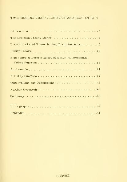
Introduction 2
The Decision Theory Model 3
Determination of Time-Sharing Characteristics 6
Utility Theory 12
Experimental Determination of a Mult i- Dimensional
irtility ^"unction 18
An Example 27
A Utility Function 34
Observations and Conclusions 44
Further Research 48
Summary 50
Bibliography 52
Appendix Al
G33892

TIME-SHARING CHAHACTEHISTICS AND USER UTILITY
by Jen-old M. Grochow
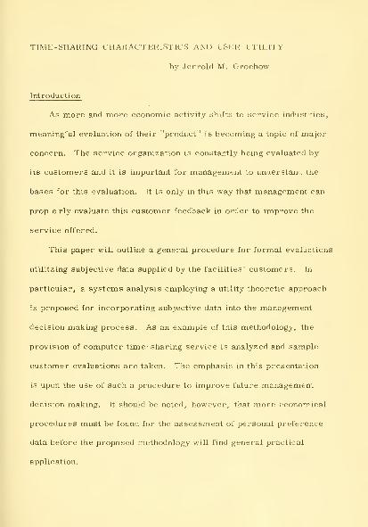
Introduction
As more and more economic activity shifts to service industries,
meaningful evaluation of their "product" is becoming a topic of major
concern. The service organization is constantly being evaluated by
its customers and it is important for management to understand the
bases for this evaluation. It is only in this way that management can
prop e rly evaluate this customer feedback in order to improve the
service offered.
This paper will outline a general procedure for formal evaluations
utilitzing subjective data supplied by the facilities' customers. In
particular, a systems analysis employing a utility theoretic approach
is proposed for incorporating subjective data into the management
decision making process. As an example of this methodology, the
provision of computer time-sharing service is analyzed and sample
customer evaluations are taken. The emphasis in this presentation
is upon the use of such a procedure to improve future management
decision making. It should be noted, however, that more economical
procedures must be found for the assessment of personal preference
data before the proposed methodology will find general practical
application.

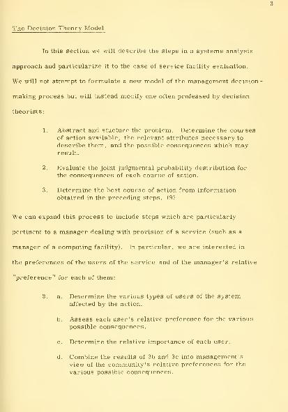
The Decision Theory Model
In this section we will describe the steps in a systems analysis
approach and particularize it to the case of service facility evaluation.
We will not attempt to formulate a new model of the management decision
making process but will instead modify one often professed by decision
theorists:
1. Abstract and stucture the problem. Determine the coursesof action available, the relevant attributes necessary to
describe them, and the possible consequences which mayresult.
2. Evaluate the joint judgmental probability destribution for
the consequences of each course of action.
3. Determine the best course of action from information
obtained in the preceding steps. (9)
We can expand this process to include steps which are particularly
pertinent to a manager dealing with provision of a service (such as a
manager of a computing facility). In particular, we are interested in
the preferences of the users of the service and of the manager's relative
"preference" for each of them:
3. a. Determine the various types of users of the systemaffected by the action.
b. Assess each user's relative preference for the various
possible consequences.
c. Determine the relative importance of each user.
d. Combine the results of 3b and 3c into management'sview of the community's relative preferences for the
various possible consequences.

If we particularize our problem to those of the computer center
manager charged with the provision of a time-sharing service, we can
now describe our model for decision making in this area:
1. a. Determine the various courses of action available to
improve service. For instance, hiring programmers,purchasing a disk drive, producing a system manual,refurbishing the computer room, etc. (This deter-
mination should take account of the various constraints
on resources such as budget or the job market. )
b. Determine the relevant attributes necessary to describethe consequences of these actions. For instance, systemavailability, reliability, response time, cost, or usability.
(These should be broken down to a level where adequatemeasures of each characteristic can be determined.For example, system availability might be measured bythe probability of a successful login, but this in itself
might have component measures relating to systemreliability and system capacity. )
c. Determine possible consequences for each course of
action. For instance, increased reliability by duplicating
equipment, decreased response time by hiring a pro-grammer (who improves the software), improved usability
by writing a new manual.
Evaluate the manager's joint judgmental probability distribution
for the magnitude of the consequences of each course of action.
How likely is it that the additional programmer will improve the
software and by how much?
a. Determine the various categories of users affected bya particular decision. For example, problem-orientedusers, students, sub-system designers, administrative
production users, etc.
b. Access each user group's preference ordering for the
various consequences of each action. (We assume that
user groups can be formed, each with a characteristic
utility function.)

c. Determine the importance of each user group (as
seen by the manager) in the particular case. Forexample, a user group dependent upon a particular
feature may be said to have a more important view-point in regard to decisions affecting that feature.
Another example would be the relatively high im-portance of student opinion in decisions affecting
computer-aided instruction or other educationaluse.
d. Combine the results of 3b and 3c to arrive at a
management preference ordering of consequences of
each of the actions.
4. Determine the best course of action from the informationobtained in the preceding steps.
These steps form the basis for the formal evaluation procedure.
In practice, management of the service facility should be able to deter-
mine, in general, relevant attributes and characteristics of the system
necessary to evaluate the consequences of any proposed action (including
the status quo) as in step lb. In the next section we show the results
of carrying out this step for the case of the time-sharing service
facility. Steps Ic, 2 and 3a must be carried out in the framework of
making a particular decision. Step 3b, however, can be performed in
some general sense by determining user preferences for different
levels of the characteristics determined in step lb. That is to say,
if we know that a user group has a low preference for a decrease in
a particular characteristic, then by implication their preference for
any action resulting in this effect will be low. The following sections
of this paper describe procedures that can be used to carry out this
analysis. A section describing the relevant concepts in decision theory
precedes the procedural description.

Determination of Time-Sharing Characteristics
Review of the literature shows a number of studies concerned
with measurement of the usefulness of time-sharing systems (4, 5, 8, 14,
15, 16, 18, 19, 20). Most simply chose system characteristics for study
on an empirical basis and did not attempt to structure or relate them to
show the analytical basis for the selection of any particular set. Miller (13),
while not specifically concerned with computing systems, does establish
a system for hierarchically relating the various system characteristics
used in his study. He. however, goes to great pains to ensure mutual
utility independence among characteristics included in the set (See
Chapter 11 of Reference 13) - something not required in this study.
The following list of time-sharing characteristics is a combina-
tion of those presented in the references indicated:
Ability to let user feel "in control"
Ability to manipulate large data bases
AccountingAvailability of terminals
BackupBatch Facility
Bulk I/O
CapacityCost
Debugging and editing systemsDocumentation
File protection, storage, and maintenance
Flexibility

Human interface
LanguagesLibrary routines
Machine independence of user programs
Output rate
Reliability
Response time
System availability
System down time
Time to learn the system
(A number of these characteristics appeared in several studies in slightly
different forms. )
Drawing upon work in a previous paper by the author (8), we will
structure these characteristics in a hierarchically related manner. On
the "top" level, the general categories of accessibility, usability, and
manageability are established. As shown in Table 1 all the characteristics
(or variants) fall either one or two levels below these general categories.
The hierarchical structure of system characteristics was deter-
mined on the basis of relatedness, importance, and inclusiveness of
the characteristics. The major divisions ( accessibility, usability,
manageability) indicated the nature of the general goals of providers of
computer service. It is possible to classify their actions in managing
as influencing one or more of these goals. The placement of system
characteristics under one of the three major headings was aided by
breaking each goal into a number of subsidiary goals (for instance.


HI
'^ ^
H m|
V. ^
o ^
OJ


accessibility into availability and approachability) which comprise
it. The choices of subsidiary goals and their placement (see Table 1>
are probably not uniquely determined but represent one possible
set which accommodates a structured listing of system character-
istics. These characteristics were analyzed for their major com-
ponent in terms of contribution towards a goal and placed in the
structure accordingly.
Establishing measures for these various characteristics is
largely a matter of determining how each system treats them. For
example, availability of terminals could be measured by the percent
of time free or by the waiting time to use them. Reliability could
be measured by the number of service interruptions (or perhaps by
the mean time between failures^ and the recovery rate of work per-
formed (or by the mean amount of work lost per failure). Data does
exist for a number of systems on parameters such as these and
user preferences for different values can be found (see below).
Such other characteristics as languages or debugging and editing
facilities, however, require both a numerical (objective) and a
qualitative (subjective) measure. Subjective measurement of these
characteristics requires user interviews ( with considerable
attention to bias elimination caused by the user's preference for
the particular value present at the time). The subject of subjective
measurement is treated in a number of papers including references
12, 13, 18, and 22.


11
In order to demonstrate the methods of utility function
determination and analysis, we will work with only two sub-goals.
While it is theoretically possible to begin an analysis of the entire
problem (that is, of all characteristics listed in Table 1), it
should be noted that only those sets of characteristics which are
expected to be affected by a particular decision (action) need
enter into the discussion. In essence, we are calculating utility
functions with certain parameter values held fixed. As will be
seen below, this technique is perfectly valid if the subject has
been properly introduced to the situation.
The two sub-goals in our analysis, availability and response
time, subsume four system characteristics:
Reliability
Capacity
Response time to trivial requests
Response time to compute-bound requests
Further, reliability has been found to be such a dominating char-
acteristic (if it is at a low value very little else matters to most
users) that we will assume it at a uniformly high level for the
remainder of our analysis. Thus, from Table 1, we see that
we will be determining utility functions with the following three
parameters:

Probability of successful login when the system is up
Real time to respond to "edit" requests
Real time to respond to "compile" request.
Table 1 indicates possible measures for a number of other characteristics
which could be used if the utility function approach were to be expanded
to many dimensions. It is felt that the characteristics chosen and
their respective measures will serve to illustrate a number of pertinent
points in the analysis. The next section deals with the theory and history
of multi-dimensional utility function assessment and will lead us into
a discussion of the actual experiments.
Utility Theory
An early paper by Yntema and Klem (24) deals with the problem of
machine evaluation of alternatives. They devise an experiment to assess
a formulation for a person's utility function involving three attributes.
The formulation was as follows:
U(x, y, z) = A + Bx + Cy + Dz + Exy + Fxz + Gyz + Hxyz (5)
This initial formulation was chosen empirically to "allow the three
attributes to interact, although only in certain restricted fashions".
The subjects in this experiment were pilots evaluating the safety
of various landing situations. The attributes under investigation were
ceiling, visibility, and the amount of fuel left on landing. They were
given a set of triples containing a particular value for each of the
attributes and told to arrange them in a preference ordering according

to the safety that the situation represented. They were told to place
chips down on a scale such that the ratio of the distances between them would
indicate the relative safety of the situations indicated on them. By
providing the pilots with chips representing the eight possible "corner"
situations (that is, the combinations of highest and lowest values of
visibilities, ceiling and fuel) the experimenters were able to evaluate the
eight constants in Equation 5. They noted that "this formula is equivalent
to a linear three-way interpolation of the kind commonly done in using
a table of a function of three variables". There was, at this time, no
justification for this functional form but a statistical analysis of machine
predictions for randomly selected triples compared very favorably with
the actual pilots' assessed safety of the situation.
Keeney, in his Master's thesis (see 9),formalized the method of
"interpolation between the corners" illustrated above. Keeney spoke of
the fact that previous discussions of multi-attributed utility functions
took the approach of assessing them as separable or additive. For two
attributes, this could be written as follows:
U(x,y) = U(x,0) +U(0,y) (6)
This functional form places constraints on the utility function that are
not often true in practice. Keeney suggests the quasi- separable utility
function as an alternative approach:
U(x,y) = U(x,0) + U(0,y) + klKx, 0)U(0, y) (7)
He then brings in the "quasi-separability assumptions" in terms of
preferences for lotteries:

< X < x=: < y < y^
(x, y) ^-vy
(x^y)
(x,y)
(0,y)
(x,rO
(x,0)
The assumptions are that there is some probability, p , such
that (x,y) for certain is indifferent to (x-'=, y) with probability p and
(0,y) with probability (1-p ). An analogous situation is shown in the
second lottery.
It is now possible to write down simple utility equations from
these two loterries to evaluate the constant k in Equation 7.
U(x,y) = p (x)U(x=.-,y) + [1 - p (x)]U(0,y) (8)
U(x,y) = p (y)U(x,y*) + [1 - p (y)U(x, 0) (9)
If we set:
U(0, 0) = U(x*,y=;0 = 1 (10)
We can then combine Equations 4 and 5 to solve for "k":
U(x,y) = U(x,0) + U(0,y)
. l-|U'x^O).U(0.y.»]„(,_„)„<„_ y,
U(x-,0)U(0,y-)
(11)

In words, the quasi-separability assumptions state that "the decision-maker's
relative preferences for different amounts of one factor are not affected
by common amounts of the other factor".
With the extension of the quasi-separability assumptions to utility
functions of three attributes, it can be shown that the formulation of
Yntema and Klem in Equation 5 is, in fact, a quasi-separable utility
function.
Later work by Keeney in his doctoral dissertation (10) formulates the
conditions for "utility independence" and shows the quasi-separability
conditions to be those of mutual utility independence. For example, an
attribute x is said to be utility independent of an attribute y if the relative
utility for values of x is independent of the value of y:
U(x,y) = C^(y) + C2(y)U(x,y^), all y (12)
It should be noted that "x utility independent of y" does not necessarily
imply "y utility independent of x". However, if both of these conditions
hold, then the utility function is separable as in Equation 7 above and
x and y are "mutually utility independent". (The conditions of utility
independence correspond to Haiffa's formulation of "strong" conditional
utility independence (17).'>
In dealing with utility functions of more than two attributes, it is
possible that attribute x is utility independent of y but not of z, or that
there be any other combination of utility independent or non-independent

variables. Kecnoy shows that it is possible to make use of any information
on utility independcuice that is available to simplify the utility func'tions.
For instance, if we have a situation where x is utility independent of
(y, z) and (y, z) is utility independent of x, then we can formulate a
utility function of vector attributes as follows:
A = (x) B = (y, z) (13)
We see immediately that our three attribute utility function, under
the above conditions, reduces to a two attribute quasi-separable utility
function with vector arguments A and B.
Keeney's work goes on to show minimal combinations of preference
curves, point utilities, or marginal utilities that can be combined with
the various conditions of utility independence in order to evaluate the
utility function over the entire space. For example, if we have a utility
function of three attributes, U(x,y, z), such that attribute x is utility
independent of (y, z) and attribute y is utility independent of (x, z), then
the complete utility function is specified by assessing six one attribute
conditional utility functions : U(x,y ,z ), U(x , y, z ), U(x ,y ,z),•^
-^o o o -^ o o • o
U(x ,y, z), U(x.^,y ,z), and U(x, y, z) for arbitrary values x , x,
y , y , and z , subject to consistent scaling on the six. The proof of
this statement follows directly from successive application of Equations 12
and 13 for the different variables. The total utility function of x, y, and
z will then be a weighted sum and product form of the six conditional
utility functions (see Reference 10, Chapter 3 for a mor-e complete

17
discussion).
l''urther statements by Keeney indicate the usefulness of the above-
mentioned techniques even under conditions of only approximate utility
independence. He shows that when Equation 12 is solved, the resulting
equation is a utility function with five degrees of freedom:
U(x,y) = U(Xq, y)[l - U(x, y^)] + U(xj, y)U(x, y^)
U(xo, yg) ' 0; U(Xj, y^) = 1 (14)
Using the techniques shown in Equation 13, we can then use this utility
function as an approximation to one with greater than two scalar attri-
butes (this is viewed as being of major importance in many operational
situations, see below).
Winkler (22) and Keeney (10) both spend significant amounts of time
discussing the procedures by which a subject should be interrogated
about his probability and utility assessments. Both stress the importance
of explaining the axioms of rational behavior and coherence. Subjects
should be made aware of any violations of these rules and given a chance
to review their assessments and remove inconsistencies.
In another work by Winkler (23), the topic of discussion is combining
the subjective probability distributions of many assessors. Various
theoretical approaches such as weighting of judgments according to the
experimenter's subjective feelings about the assessor, or according
to the subject's own feelings about his expertness in this situation.

18
are discussed. Various behavioral approaches to the problem, such
as feedback and reassessment by each subject, or group reassessment
of probabilities are also discussed. Winkler states that "the discussion
indicates that different methods may well produce varying results. Of
course, there is no correct weighting function, so it is impossible to
select ainetod because it is more nearly "correct" than other methods".
If we assume that the ultimate aim of the assessment procedure is
to make a decision about a multi-attributed situation, then the importance
of Winkler's work is in allowing us to test the sensitivity of the decision
to different weightings of subjective judgments. In the final analysis,
this work is meaningful only so far as "mechanical rules simplify the
decision-maker's problem and at the same time seem reasonable to
him."
Experimental Determination of a Multi-Dimensional Utility Function
The management decision-making procedures outlined in the
beginning of this paper hinge upon successful determination of user
utility functions. An experiment was performed to show the feasibility
of this determination for one group of users of a general purpose
time-sharing system. The experiment consisted of a series of
interviews with users to determine the minimum amount of information
necessary to formulate their utility function. The determining
factor as to what information was necessary was the utility independence
relationships that existed among the system characteristics (see the

discussion in the previous section). The data was then combined
according to the mathematical formulation of the utility function
and tested for general correctness (no statistical tests of accuracy
were made as the usefulness of these procedures does not rely upon
extreme precision of utility values).
The interview procedure consisted of several parts:
1. General determination of users' usage patterns of
the time-sharing sei-vice.
2. Introduction to basic theory of utility assessment.
3. Focusing of attention on the three attributes to be
discussed: availability, response time to trivial
requests, and response time to compute-bound
requests.
4. Determination of utility dependence relations.
5. Determination of conditional utility functions and
point utilities necessary for the calculation of the
total (three-dimensional) utility function. (Which
conditional and point utilities were needed was deter-
mined by application of mathematical utility theory.
All assessment procedures are based on the assumption that
the subject can abstract his feelings regarding the comparison of
situations which are not occurring at the present time. It is fairly easy
to show that while such assessments for situations which the subject
has experienced in the past require a good deal of care, determining

20
preference data for situations which he has not experienced becomes
increasingly difficult to validate and reproduce as the hypothetical
situation becomes more removed from the subject's experiences.
For this reason, general conversations about the types of work that
the subject performed on the time-sharing system were held prior
to any assessment procedui'es. If, for example, the subject had
never experienced extreme values of the variables to be assessed,
then efforts were made to delay further analysis until these exper-
iences occurred. Another approach to this problem would have been
to simulate certain conditions during test periods when the user was
active on the time-sharing system.
As mentioned earlier, another factor that is felt to be impor-
tant in performing judgmental assessment procedures is the intro-
duction of the subject to the theory and methodology. For this reason
some simple everyday situations were analyzed with the various
subjects before discussion of their utilities for the characteristics of
the time-sharing system. In these discussions, points were made
relating to "rationality", particularly as it pertained to the meaning
of independence of variables and the transitivity of preference state-
ments. Throughout the procedures, any inconsistancies in assessments
found were discussed with the subject to determine whether they could
be removed upon reassessment.

21
Focus was then directed to the three attributes to be con-
sidered by presenting a scenario which established their presence
as the major variables. For instance, the question of reliability
was removed from the picture by insuring that on the "experimental"
time- sharing system it was at a uniformly high level as stated above,
(as long as this situation was not too far removed from the user's
experiences it was felt that he could and would accept the assump-
tion and thus ignore reliability as influencing his preferences
V
Another example is that the features necessary for him to adequately
perform his task were assumed to be fully operable (again, it was
necessary thatthis condition not be too far removed from actuality^
In essence, we were, therefore, computing utility functions conditional
on high levels of all characteristics that were not explicitly considered.
Independence relations were determined by a series of
questions regarding the shape of various conditional utility curves.
For example, if the user asserts that his conditional utility function
for availability has one shape when response time is at a favorable
level and a fairly different shape when response time is at an un-
favorable level, then we can say that availability is not utility indepen-
dent of response time. If, on the othei- hand, the user asserts that
the shape of his conditional utility curve for one variable is indepen-
dent of the value of the second variable, then we can state that a
utility independence relation exists. The utility independence


22
relations were then used to determine a mathematical form for a
complete utility function (as shown in the section on theory^ involving
a relatively small number of conditional utility functions and point
utilities.
The final step in the procedure is the actual determination of
conditional utility functions and point utilities as indicated necessary
for the calculation of the entire utility space. If a sufficient number
of independence relations exist, the conditional utility functions to
be determined are in fact functions of only one variable. A person's
relative preferences for values of a single variable can be assessed
in several ways including the presentation of "lottery" situations and
by "fractile assessment". In the lottery assessment procedure a
typical question might appear as follows:
At the beginning of each month, you are given the
opportunity to be assured successful logins x percent of
the time, or to participate in a lottery, which gives you
a certain probability of assuring all successful logins for
the month and a certain probability of refusing you service
for the month. That is to say, we are offering guaranteed
success of login of x percent per month or the opportunity
to try for a chance at 100 percent successful logins during
the month. If you try for the chance at 100 percent success-
ful you are risking the receipt of percent. The lottery is
a fair game and we will tell you in advance what the probability
is that you will "win" (receive 100 percent successful
logins during the month). For what value of this probability
will you be indifferent between participating in the lottery
or receiving immediate assurance of x percent of successful
login?

23
This situation is presented, with discussion, for a number of
different values of x in order to determine relative preferences for
the values of the variable "probability of successful login. "It was
found, however, that a number of subjects had difficulty in placing
themselves in the "lottery" experience and for them a method of
fractile assessment was used. A typical presentation would then
be as follows:
Time-sharing service is contracted for in terms of anassures "probability of successful login". This can rangefrom percent (no service during the month) to 100 per-cent (guaranteed service at any time). What percentageof successful logins is worth the miost to you? (This maybe 100 percent or less than 100 percent if the person doesnot require guaranteed service. ) What is the maximumpercentage for which the service is useless? (This maybe above percent for people who require a minimum gradeof service. ) Now try and find a percentage for which the
service would be worth half as much as it would at the
maximum value. This is the . 5 fractile. For what peix-entage
would service be worth three quarters as much, one quarteras much, etc. ?
Since the meaning of the word "worth" is not entir-cly clear,
many subjects immediately fall into thinking about a monetary
equivalent. Since it is established that the maximum amount of


24
money ever to be paid will be no more than their current expenditure,
it is assumed that money is a reasonable proxy for worth and that its
use does not introduce any additional non-linearities in the assessment
procedures. (In general, this assumption cannot be made and tests
must be performed to determine the user's utility for different amounts
of money. What we are assuming is that these utilities are linear over
the particular range. )
In order to insure that the one-dimensional utility functions
assessed as above are in fact conditional utility functions for the ap-
propriate specific values of the other variables, the experimenter
first presented and discussed with each subject the environment (that
is, values of all other variables) in which he was being asked to assess
a one-dimensional utility function. For example, if he were asked to
assess utilities for probabilities of login (as indicated in the sample
questions above) then he would be asked to assume a response to trivial
requests and a response to compute-bound requests as suggested by the
experimenter. It can be seen, therefore, that the user must be asked
to assess a particular utility function (say for probability of login)
under a number of different sets of environmental conditions (different
values of the other variables). The total number of conditional functions
that must be assessed is determined by the types of independence:
relationships that exist between the variables. (The next section of
the paper will show an example of this assessment and will re-emphasize
these points. )


25
Finally, the user was asked to assess his utility for the eight
possible "end points" generated by the combination of the highest and
lowest values of the three variables. The method used for this assess-
ment was very similar to that of Yntema and Klem (24) mentioned above.
The eight possible end points were calculated and each was written on
a separate paper marker. The subject was given simple scale on which
to lay the markers according to their relative value to him. He was told
to place a marker so that the distance from the base line represented
his assessment of the "value" of the service quality specified by the
indicated values of the variables. He was told that if the distance from
the base line for one marker was twice the distance from the base line
for another marker, then this should indicate that the quality of the
situation represented by the first marker was twice the quality of the
situation represented by the second marker. This procedure produced
information for the determination of the total utility function by providing
scaling points and fixing origins.
It should be noted that while all of these steps could be carried
out sequentially, the experimental procedure was very iterative in
nature: for instance, if determination of a conditional utility function
showed a possibly incorrect utility independence relation, than this
part of the procedure was redone. A number of interviews were held
with selected users to ensure the validity of these results. Much general
discussion was interspersed with the assessment procedure to give the


26
users a chance to "live with" their statements, understand the implica-
tions of other assessments, etc. Although time consuming, this is an
important part of the assessment procedure. It is in this way that the
experimentor attempts to ensure that all extraneous factors are removed
from the assessment. In the next section we give an example which
shows specific utility independence relations and the calculation of a
total utility function.

27
An Example
The users interviewed were computer system application
programmers whose main tasks were the input and editing of pro-
grams (trivial requests) coupled with compilation and testing
thereof (compute-bound requests). The ratio of editing sessions
to compile and testing sessions was fairly high (about five to one'>
indicating that a lot of "desk debugging" was being done (somewhat
irrelevant to the problem, but interesting nonetheless). Initial
testing of the subjects indicated the following utility independence
relationships between two variables when the third variable was
in the relevant range:
1. RT ui (utility independent) A - Relative preferences
for trivial request response time was independent of availability.
2. RT ui RC - Relative preferences for response to
trivial requests were independent of response to compute-
bound requests.
(These both seem to make sense since response time
to editing requests was the major determinant of how
much work could be accomplished. It is suspected

28
that these may not hold for other classes of users -
especially when there is a more even balance between
trivial and compute bound requests. )
3, RC ui A - Relative preferences for compute bound
response time was independent of availability.
(This also seems reasonable, as the subjects, in
general, tended to separate preferences for the various
values of system work conditions from anything else.
This may also not hold for a less demanding user type. )
This, of course, leaves the following three pairs to be not
utility independent:
A. A not ui RT,
B. A not ui RC, and
C. RC not ui RT,
(Again these seem to make logical sense, as indicated
in the following statements. If either response has
an unfavorable value, then the relative preferences
for A may very well change as the programmer will
spend most of his time having to contend with the
unfavorable response and may not wish to log in
as badly. Also, in any particular session, the
programmer may set his relative

29
expectations for RC in terms of the RT he is experiencing -
a not uncommon practice of changing sights in view of
concurrent conditions. )
It was now possible, using similar methods to those developed by
Keeney (10), to determine exactly which conditional utility functions
and point utilities had to be determined to completely specify this class
of users' complete utility function. The following was proven:
Given the above conditions of utility independence of the three
attributes A, RT, HC, the following four utility points and seven one-
attribute conditional utility functions are sufficient to completely specif;y
U(A, RT, RC):
Point utility for (A RT RC ) and (A RT , RC ), (A, RT RC ),
(A , RT , RC ), as well as scaling points for minimum and
maximum utility.
Conditional utility functions: U(A, RT , RC ), U(A, RT , RC ),
U(A, RT RCq), U(A, RT RC ), U(A , RT, RC^), U(A^, RT^, RC),
and U(A , RT,, RC).1 1
The utility function thus obtained is as follows:
U(A, RT, RC) = |u(A, RTq, RC )
+ [U(A, RTq, RC^) - U(A, RTq, RCq)]
U(Aq, RT, RCp)
U(A RTq, RC) - U(A^,RTq,RCq)
U{A^, RTq, RC^) - U(A^,RTq,RCq)
^i\, RT^, rCq) ) Cont.

30
+^U(A, RT^, RC ) + [U(A, RT^, RC^) - U(A, RT RC )]
U(A RT RC) - 1
U(A RT RC ) - 1
U(A RT, RC )
U(A^, RT^, RC^)(15)
The complete proof of this theorem is provided as an Appendix to this
paper. The points and conditional utility functions indicated are shown
graphically in Figure 1.
The above equation is not a unique determinant of the utility function
as is shown below. The theory allows us to derive several equations,
each of which is an equivalent statement of the utility function. For
example, a slightly different derivation (see the Appendix) yields a
function that can be specified by the following point and conditional utilities
(see Figure 2):
Points: (A RT RC ), (A RT RC ), and (A RT RC ) and
scaling points.
Conditional utUity functions: U(A, RT RC^), U(A, RT^, RC^),
U(A, RT RCq), U(A, RT RC ), U(Aq, RT, RC^),
U(Aq, RT RC), andU(A^, RT^, RC)
which yield a utility equation as follows:
U(A, RT, RC) =
LI (A, \\T^, RCq)U(Aq, HT^. RC)
U(Aq, RTq, RC^)
+ U(A, KTq, RC^)IJ(Aq, RT^, RC)
U(Aq, RTy, pxy
Cont.

31
(Aj.RTq,RC^)
(Aj.RTq,RCj)
(A^,RT^,RCq)
Figxire 1
Points and one-dimensional utility functions necessary to
evaluate utility values within the cube under following utility
independence relations: RT ui A
RT ui RC
RC ui A

32
(Aj,RTq.RCJ,
(Aj,RTq,RCj)
(Aj,RTj,RCq)
RT
O-RTj^RCq)
(Aq^RTj.RCj)
Figure 2
Possible alternative requirements for calculation of utility
space having independence relations: RT ui A
RT ui RC
RC ui A

33
1 -
U(Aq, RT, RCq) )
+ ^U(A, RT , RC ) 1 -
U(A RT RC) - 1
U(A^, RT^, RCq) - 1
+ U(A, RT RC )
U(A RT RC) - 1
U(A^,RT^.RCq)
(U(A^, RT, RC^)
)
(U(A^, RT^. RC^))(16)
We can now see that the determination of a three-dimensional
utility function for this class of users has been reduced to the determination
of several (conditional) one-dimensional utility functions and point
utilities - a fairly simple assessment process for both experimenter
and subject.
By using a similar procedure for each class of users (and remembei",
we predict that this will be a numerically small number), we can
effectively determine utility functions for the entire user population.

34
A Utility Function
Figures 3 through 9 show computer generated plots of conditional
utility functions derived from Equation 15. A time-sharing user whose
main job was programming was interviewed (as described above) for
the purposes of assessing actual point and conditional utility functions
and /or determining the appropriateness of the utility independence
relationships specified. After appropriate scaling (to bring utilities
in the range to 1000), the utility space was generated. The utility
value is shown on the z coordinate and the two variable characteristics
on the X and y. The third characteristic is held fixed as indicated.
The first plot (Figure 3) shows the user's utility for various
values of response to trivial requests (RT) and response to compute
bound requests (RC) when availability is at its maximum value (100%
probability of login). As can be seen, the relative preferences for
RT (that is, a conditional utility curve for RT) is independent (has
the same shape) for all values of RC. On the other hand, it can also
be seen quite clearly that the shape of conditional utility curves for RC
vary as RT goes from its maximum to its minimum value. By noting
the relative magnitude in change of utility between one set of values
for RT and RC and another set of values, the decision-maker can
determine where the greatest marginal improvement will occur. He
might use this information to help him select the alternative which best
assured him of the appropriate changes in the values of those charac-
teristics.

35
U= 1000
U(A= 1.0, RT, RC)
U= 500
RT
|U= 750
RC^
Figure 3
Utility space calculated using data from point and conditional
utility functions in Equation 15 (three dimensional view shown
is for highest value of availability).

36
U(A = .5, RT, RC)
U= 250
RT
U= 383
U= 80
Figure 4
Conditional utility space with availability equal 50%,
RC

37
U(A=. 1. RT. RC)
U= 125
RT
7- U= 250
'~U= 250
RC
Figure 5
Conditional utility space at minimum value of availability.

38
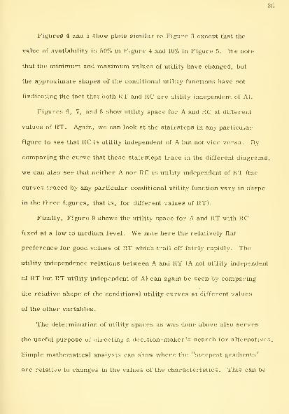
Figures 4 and 5 show plots similar to Figure 3 except that the
value of availability is 50% in Figure 4 and 10% in Figure 5. We note
that the minimum and maximum values of utility have changed, but
the approximate shapes of the conditional utility functions have not
(indicating the fact that both RT and RC are utility independent of A).
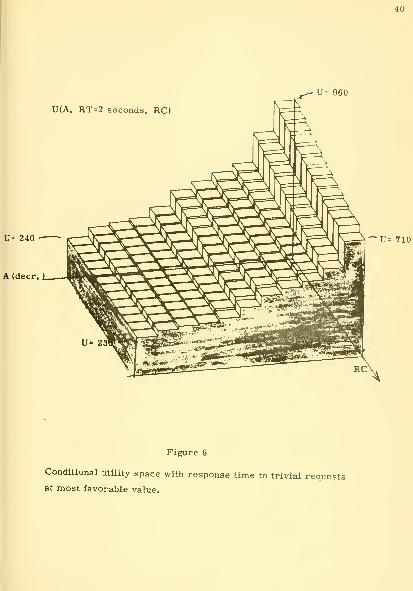
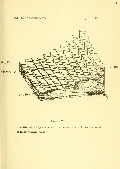
Figures 6, 7, and 8 show utility space for A and RC at different
values of RT. Again, we can look at the stairsteps in any particular
figure to see that RC is utility independent of A but not vice versa. By
comparing the curve that these stairsteps trace in the different diagrams,
we can also see that neither A nor RC is utility independent of RT (the
curves traced by any particular conditional utility function vary in shape
in the three figures, that is, for different values of RT).
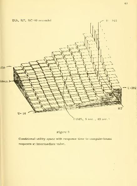
Finally, Figure 9 shows the utility space for A and RT with RC
fixed at a low to medium level. We note here the relatively flat
preference for good values of RT which trail off fairly rapidly. The
utility independence relations between A and RT (A not utility independent
of RT but RT utility independent of A) can again be seen by comparing
the relative shape of the conditional utility curves at different values
of the other variables.
The determination of utility spaces as was done above also serves
the useful purpose of directing a decision-maker's search for alternativos.
Simple mathematical analysis can show where the "steepest gradients"
are relative to changes in the values of the characteristics. This can be


39
combined with the manager's knowledge of the probable consequences
of vai-ious actions to arrive at a set of possible policies which would he
most advantageous to users of the computation facility. Further
exploratory work needs to be done in this area as well as others to
be described below.

40
U= 960
U(A, RT = 2 seconds, RC)
U- 240
A (deer,
U- 710
Figure 6
Conditional utility space with response time to trivial requests
at most favorable value.

41
U(A, RT-5 seconds. RC) U- 740
l]= 185
'^{decr. )
U= 120
— U= 490
Figure 7
Conditional utility space with response time to trivial requests
at intermediate value.


42
U(A, RT=9 seconds, RC)
.- U - 540
U- 290
U= 20 — RC
Figure 8
Conditional utility space with response time to trivial requests
at least favorable value.

43
U(A, RT, RC = 40 seconds) U - 915
U= 16
U(50%, 5 sec. . 40 sec. 1
Figure 9
Conditional utility space with response time to compute-bound
requests at intermediate value.


44
Observations and Conclusions
The experimental determination of a utility function of three
par-ameters was successfully accomplished as outlined above. This
procedure, however, as complex and time consuming as it was, is
only part of the general management decision-making process
described in the beginning of this paper. It is still necessary for
the manager to determine various possibilities for action and the
presumed affect of these actions on the characteristics of the service.
The calculation of a user's utility function is simply a tool
for prediction of what the reaction of the community will be to the
manager's decision. Since the manager is concerned with a number
of user groups and with other factors as well (such as top management
requirements, etc. ), a single utility function is only a small part of the
data needed to make a decision. If a user's utility function could only
be used in this way, then we would question whether the effort was
justified. However, it is often argued that perhaps the largest part
of any manager's time and intellectual activity is spent in the process
of "problem finding" (26). If the utility function could be used in this
area as well, it would gain additional value. Similarly, Simon (21) has
indicated that the problem solving activities of "intelligence" and
"design" occupy a proportionately larger share of the total problem
solving time and effort than does the final "choice" for a large class
of problems. We will show in the next few paragraphs how the user's

45
utility functions can be used in searching for problems and for
alternatives as well as in making a final decision. We assume
below that the utility function depicted in the preceding diagrams
represents the only user group that our h3rpothetical manager
has to deal with.
In the first case we wish to see if there is any way that
existing resources can be used to provide better services. For
example, there is a general relationship between the number of
users of a time-sharing system and the response time. If we
currently set the maximum number' of users at the value n, we
can then measure the response time to trivial requests, r.
Generally, by setting a lower value for the maximum number of
users we will achieve a decreased response time (basically, because a
smaller number of users will be demanding a smaller amount of
the total system's resources). The question is whether that is
a desirable thing to do in terms of increasing user utility, and if
so, at what point should we stop. If we look, for instance, at
Figure 9 and assume some current operating point of A ^ 50% and
HT = 5 seconds, we can then determine that moving to a point
(40%, 4 seconds) has approximately the same utility value where
(40%, 3 seconds) has a significantly higher utility value. Similarly,
moving to a point (60%, 6 seconds) has a lower utility value and
(70%, 6 seconds) has a higher utility value (although not as high

46
as (40"/(), 3 seconds)). Thus, if our present resources can be
arranged to take us to one or the other of the better operating
points (or some other operating point that has a higher utility
value), then we have improved our- overall service at no additional
cost. Similar analyses can be done for other variables as well.
Tf we now take the situation where an additional amount of
money is to be spent and the determination of which resource to
spend it on is in question, then we can again use the utility function
to help us in our decision. If we look at oui- operating point in
the overall utility surface, it should be possible to mathemati-
cally determine the direction of "steepest gradient" (fastest
increase in utility value). We can determine "feasible" directions
according to the characteristics which can be modified by the
application of further resources (we may be able to change avail-
ability to some degree, response time to trivial requests to another
degree, and response time to compute-bound requests not at all--
therefore I'uling out certain directions of moving). Finally, we can
then compute that point in the feasible r-egion which provides the
greatest utility increase (this procedure is very similar to some
used in the solution of non-linear progr-amming problems). With
the aid of the computer the mathematical manipulations may be
fairly easily performed.

47
As utility assessment procedures become more widely used
and accepted, we expect even fur-ther investigation of the use of
utility functions as major policy r-eassessment tools. We have
indicated in this papar several ways in which the use of user
determined utility functions can enter into all stages of the manage-
ment problem finding-decision making process. If further work
in this area makes it easier to extrapolate the fairly simple example
discussed above to problems involving numerous characteristics
and several groups of users (and hence, several utility functions^,
we see general applicability of these techniques. The management
of service facilities is a sufficiently important problem so as to
almost guarantee the interest of researchers and practitioner-s
alike in these areas. We look forward to the extension of this
work in the near future.

Further itesearch
The major dcterTcnt to the use of multi-ciimensional utility
calculations for management decision-making is in establishing the
reliability of the utility assessment and in the relative cost of the
assessment procedure. Management problems are characterized
by a
1. large number of relevant variables
2. small number of utility independence relations
3. large number of conditional utility curves with
thresholds, "knees", or other irregularities
all of which serve to increase the number or complexity of the utility
points or conditional functions which must be assessed in order to
specify the complete utility function. Assessment procedures current-
ly require laborious and painstaking work to ensure the validity of the
assessed values - work that, in general, must be repeated for each
service facility user being interviewed.
Research areas which would foster the acceptance of the utility
approach to complex managerial decision-making currently include:
1. "Assessment by questionnaire. " If adequate questions could
be formulated to cut down significantly on interviewer time,
utility determination could be integrated into existing manage-
ment infor-mation gather-ing procedures.

I
49
2. Machine-aided assessment. The use of conversational
graphics systems should be experimented with to give
the subject a pictorial "feel" for the meaning of his
assessments. This should help increase reliability of
assessed utilities.
3. Utility function approximation and sensitivity analysis.
The issue is establishing procedures for easily deter-
mining the dominant variables and relationships in any
problem. A side effect of this could be a decrease in
number and dimension of conditional utility functions
that must be assessed.
4. User utility equivalence determination. Ad hoc procedures
were used in this paper to determine user "classes" on
the basis of similar characteristics. More work needs
to be done to make this determination more accurate.
Correlation of membership in a class (at a given time)
with the actual work performed on the service facility
should be attempted.
5. Time variance of utility assessment. How often must a
manager reassess utilities in his user community to
ensure that his data truly reflects their preferences?
Research could be devoted to controlled experiments
over time periods relevent to the service facility in
question (six months of more in the case of computer
systems - about the length of time necessary for major

50
changes).
6. Utility functions of utility functions, fn order to better
understand the utility function of managers, we need to
investigate the properties of utility functions whose
attributes are other utility functions.
Research in these and other areas should be yielding further
insights into the use of utility functions in practice in the near future.
Summary
We are concerned with the basic problem of providing a
mechanism for decision-making regarding the provision of some
service to a population of users. Problem analysis begins by
defining a hierarchy of system characteristics and measures
of effectiveness for them. By using the methodology of utility
function assessment, it is possible to determine a multi-dimensional
utility function for each group of users.
As an example, system characteristics of a general purpose
time-sharing system were determined and several user utility
functions were assessed. The decision-maker 'the Computer Center
Manager) must then go about the task of evaluating probable changes
in the various attributes due to any action he might possibly take
and determining the relative importance (to him^ of each user-
group's utility for the action. The results of these analyses can


then be combined to evaluate a "most desirable" action.
As stated earlier, it is felt that the procedures illustrated
in this paper hold considerable promise for the future. As
management must deal with more and more complex problems
with mofe variables, more "interested parties, " and more
possible actions, use of an integrated set of procedures for
evaluation of alternatives will become more prevalent, incor--
poration of Individual preference data can only increase the
depth and breadth of management understanding.

52
Bibliography
1. ]3ctaque, N.E. and C;. A. Ciorry, "Automating Judgmental Decision
Making for a Serious Medical Problem", Management Science ,
Vol. 17, No. 8, April 1971.
2. Brown, Rex A. , "Do Managers Find Decision Theory Useful?",Harvard Business Review , May-June 1970,
3. Carbonell, Jaime 1^. , Jerome I. Elkind, and iiaymond S. Nickerson,"On the Psychological Importance of Time in a Time-SharingSystem", Human Factors , Vol. 10, No. 2, April 1968.
4. Fano, Robert N. , "The Place of Time-Sharing", Engineering
Education, April 1968.
5. Gold, Michael M. , "A Methodology For Evaluating Time-SharingComputer System Usage", Doctoral Dissertation, Sloan School
of Management, M.I.T., June 1969.
6. Good, I. J. , The Estimation of Probabilities - An Essay on
Modern Bayesian Methods , The M. I. T. Press, Cambridge,Massachusetts, 1965.
7. Greville, E. M. , "The Use of Value Functions for the Comparisonof Data Processing System Configurations". Technical ResearchReport R-70-07 , Department of Electrical Engineering, University
of Maryland.
8. Grochow, J.M. , "Architectural Implications of User Needs in
Time-Sharing Service", IEEE Convention Digest , March, 1971.
9. Keeney, R. , "Evaluating Multidimensional Situations Using AQuasi-Separable Utility Function", IEEE Trans, on Man-MachineSystems , Vol. MMS-9, 1968, pp. 25-28.
10. Keeney, R. L. , "Multi- Dimensional Utility Functions: Theory,Assessment and Application", Technical Report No. 43 , Operations
Research Center, M.I.T., October, 1969.
11. Laver, Murray, "Users' Influence On Computer Systems Design",
Datamation , October 1969.
12. Luce, R. D. and J. W. Tukey, "Simultaneous Conjoint Measurement'
Journal of Mathematical Psychology , Vol. 1, 1964, pp. 1-27.

13. Miller, J. R. , III, "The Assessment of Worth: A SystematicProcedure and Its Experimental Validation", Doctoral Dissertation,
Sloan School of Management, M.I.T, , June 1966.
14. Ness, D. N., C. R. Sprague, and G, A. Moulton, "On the
Implementation of Sophiscated Interactive Systems", Sloan SchooVof Management (M. I. T. ) Working Paper 506-71 .
15. Nickerson, Raymonds., Jerome I. Elkind, and Jaime Pi. Carbonell,
"Human Factors in the Design of Time-Sharing Computer Systems",Human Factors, Vol. 10, No. 2, April 1968.
16. Nolan, R. L. , Final Report, Advanced Computer Application
Seminar, under Prof. J. McKenney, Harvard Business School,
June 1970.
17. Raiffa, H. , "Preferences for Multi-Attributed Alternatives",
RM-5868-DOT/liC, The RAND Corporation, April 1969.
18. Reventar, R. E. , "A Study of Time-Sharing Users: Their Attitudes
and Behavior", M.S. Thesis, Sloan School of Management, M.I.T.,September 1970.
19. Simon, Herbert A. , "Reflection on Time-Sharing from a User'sPoint of View", Computer Science Research Review 1966 , CarnegieInstitute of Technology.
20. Stimler, Saul, "Some Criteria For Time-Sharing System Performance",Communications of the ACM , Vol. 12, No. 1, January 1969.
21. Winkler, R. L. , "The Assessment of Prior Distributions in
Bayesian Analysis", Journal of the American Statistical Association,
Vol. 62, 1967, pp. 776-800.
22. Winkler, R. L. , "The Quantification of Judgment: Some Methological
Suggestions", Journal of the American Statistical Association ,
Vol. 62, 1967, pp. 1105-1120.
23. Winkler, R. L. , "The Consensus of Subjective Probability Distributions'
Management Science , Vol. 15, No. 2, 1968, pp. B-61 - B-75.
24. Yntema, D. B. and L. Klem, "Telling a Computer How to Evaluate
Multi-Dimensional Situations", IEEE Trans, on Human Factors in
Electronics, Vol. HFE-6, No. 1, September 1965, pp. 3-13.


54
25. Diamond, D. S. , "A Model for Information System Design,Evaluation and Resource Allocation", Doctoral Dissertation,
Sloan School of Management, M.I.T. , June, 1969.
26. Pounds, W. F. , "The Process Of Probelm Finding", Industrial
Management Review , Vol. 11, No. 1, Fall, 1969.
27. Simon, H. A. , The New Science Of Management Decision ,
Harper & Bros. , New York, 1960.

Al
APPENDIX
The following is the proof of the fesult stated in Equation 15 in the text. We wil
show that, given the utility independence relations shown below, the utility function
U(A, RT, RC) can be evaluated by the expression in Equation 21 using only the
indicated conditional and point utilities.
Utility independence relations:
RT ui A (1)
RT ui nC (2)
RC ui A (3)
Given the definitions of utility independence and mutual utility independence given
by Keeney (10), we can write the following equations:
(4)
Using (1) and (2) above:
U(A, RT, RC) = C^(A, RC) + C2(A, RC)U(Aq, RT, RC^)
for some value of RC = RC and A = A
Using (3) above, and setting RT = RT :
U(A, RTq, RC) = D (A, RT ) + D2(A, RT^UiA^, RT^, RC) (5)
for some value of A = A
Using (3) above, and setting RT = RT :
U(A, RT , RC) - E (A, RT ) + ^2''^' l^^ )U(A RT^, liC) (6)
for some value of A ^ A
We can now set the scale by assigning
U(A^, RTq, RC^) -
U(A RT RC ) = 1
(7)
By evaluating Equation 4 with RT = RT we get
U(A, RTq, RC) = C^(A, \{C) (8)

By evaluating Equation 5 with I^C ^ HC we get
U(A, KTq, UCq) = D^(A, in^^) + D^iA, 1?Tq)U(A^, HTq, RCq) (9)
and by evaluating Equation C with KC = HC we get
U(A, RT , RC ) - E (A, RT ) + E2(A, RT ) (10)
Substituting these results into our first equations, we arrive at
U(A, HT, RC) = U(A, RTq, RO+C^CA, RC)U(Aq, RT, RC^) (11)
U(A, RT^, RC) - U(A, RT_, RC.)
H-D^iA, RTq) U(A^, RTq, RC) - U(A^, RT^, RC^) (12)
U(A, RT RC) = U(A, RT RC ) + E^CA, RT^)fj(A^, RT^, RC) - l] (13)
3y setting RT = RT in Equationll, we get an expression for C^:
U(A, RT RC) - U(A, RT , RC)C (A, RC) -
U(Aq, RT^, RCq) (14)
Similarly, we set RC = RC in Equation 12 to get an expression for D :
IKA, RT RC ) - U(A, KT HC )
D (A, RT )- —U(A^, liTp, RC^) - U(A^, 1{Tq, RCq) (15)
iC ^ RC in Equation 13 to get an ex
U(A, RT RC )- U(A, RT^, RC^)
U(A RT RCq) - 1 (16)
nmilarly, we set RC ^ RC in Equation 13 to get an expression for E^
E2(A, RT^) =

Substituting these results into our last set of equations, we get
A3
U(A, KT, KC) I) (A, \{T^, ]{C)
-[lJ(A, RT KC) - U(A, HTq, HC)]°
U(Aq, KT, RCq)
U(A^, KT^, RC^) (17)
U(A, RT^, RC) = U(A, RT^, RC )
U(A, RT RC )- U(A, RT RC )
+ kj(A RT RC) - U(A RT RC )| (18)
U(A RT RC ) - U(A RT , RC )
^ ^ i u UJ
U(A, RT RC) - U(A, RT RC )
U(A, RT RC^) - U(A, RT RC^)
U(A^, RT^, RCq) - 1
[uCA^, RT^, RC) - l]
(19)
Ne rearrange Equation 17 for convenience
U(A, RT, RC) = U(A, RT RC) 1 -
U(Aq, RT, RCq)
U(A^, RT^, RCq)
+ U(A, RT , RC)TI(A^, RT, RCp)
U(A^, RT^, RC^)(20)
slow, by simply substituting Equation 18 for U(A, RT , RC) where it appears
n Equation 20, and Equation 19 for U(A, RT RC) where it appears, we get
)ur final result
U(A, RT, RC) = )U(A, RT , RC^)
[u(A, RT HC ) - U(A, RTq, RC^)"]
U(A RTq, RC) - U(A^, PvTq. RC^)
U(A^, liT^, RC^)-U(A^, HT^, I'.C^)
C(>N

A4
; U(A , RT, RC^) \
(^ U(A^, RT^, ^*^0^ '
. (U(A, RT RC ) + [u(A, RT RC ) - U(A, RT , RC )J'
U(A RT , RC) - 1
U(A^. RT^. RCq) - 1
U(A^, RT, RC^)^__o ol)
QU(A^, RT^, RC^O(21)
It can now be seen that the following point and conditional utility relationships are
sufficient to compute the utility function U(A, RT, RC) given the independence
relations in Equations 1, 2 and 3:
Point utilities: U(A^, RT^, RC^)
U(A^, RTq, RCq)
U(A^, RTq, RC^)
U(A^, RT^, RCq)
Conditional utility functions: U(A, RTq, RCq)
U(A, RTq, RC^)
U(A, RT , RCp)
U(A, RT , RC^)
U(A RT, RCq)
U(A, RTq, RC)
U(A RT RC)
fhis set of utilities is shown pictorially in Figure 1.
In order to arrive at text Equation 16 , we simply allow A = A instead of
A^ in Appendix Equation 5 and continue the analysis from there. The point and
conditional utilities necessary to calculate the utility space from this equation are
lepicted in Figure 2.

R 14 7s

^-^^

•>A^ i t ., .
•
3 TDflD 0D3 701 ffi
3 TDflO DD3 t,7Q 517HP"
iillilllilliil--
3 TOAD DD3 b7D 541
3 TDflD 003 b70 Mfi3
3 TOaO 003 701 S4I55a-7A
3 TOflO 003 701 MMS
3 TOflO 003 b70 4T1
3 TOaO 003 701 53b•Er-7Z
3 lOflO 003 b70 5Sfl
5'^fo-7^
S<g7'72
3 lOflO 003 701 4=m