Embed Size (px)
Citation preview

Time splitting for wave equations in random media
Guillaume Bal∗ Lenya Ryzhik †
January 29, 2004
Abstract
Numerical simulation of high frequency waves in highly heterogeneous media is a challengingproblem. Resolving the fine structure of the wave field typically requires extremely small timesteps and spatial meshes. We show that capturing macroscopic quantities of the wave field,such as the wave energy density, is achievable with much coarser discretizations. We obtainsuch a result using a time splitting algorithm that solves separately and successively propagationand scattering in the simplified regime of the parabolic wave equation in a random medium.The mathematical theory of the convergence and statistical properties of the algorithm is basedon the analysis of the Wigner transforms in random media. Our results provide a step towardunderstanding time and space discretizations that are needed in order for the numerical algorithmto capture the correct macroscopic statistics of the wave energy density in a random medium.
1 Introduction
Wave propagation in highly heterogeneous media has many applications such as light in a turbulentatmosphere, microwaves in wireless communication, acoustic waves in underwater communication,and seismic waves generated by earthquakes [10, 22, 31, 32]. Numerical simulations of wave equationshave been thoroughly analyzed; see, e.g., [12, 14] for recent monographs. Most numerical techniquesare adapted to the low-to-moderate frequency regime where the size of the calculation domain isnot too large compared to the typical wavelength of the system. More recent works consider highfrequency wave propagation in the semiclassical regime, which corresponds to the high frequencyregime with slowly varying underlying media [7, 25, 26].
Comparatively little is known about high frequency wave propagation in highly heterogeneousmedia. This is the regime where the wavelength is much smaller than the overall size of the propaga-tion domain while the scale of the variations in the medium is comparable to the wavelength. Suchproblems arise in many of the aforementioned applications. There, waves fully interact with themedium and the precise numerical simulation of this interaction requires computational capabilitiesthat are usually not available. Our objective is to provide some guidelines as to how to faithfullycapture macroscopic properties of the wave propagation numerically at a minimal computationalcost. More precisely we wish to devise schemes to solve the wave equation that accurately computethe wave energy density and in particular have the correct statistical properties while not necessar-ily capturing small scale structures of the wave field. These small scale details are usually of littleimportance in practice.
In this paper we restrict ourselves to a setting that is practically useful yet much simpler thanthe full wave equation so that a complete mathematical theory can be obtained. This setting is the
∗Department of Applied Physics & Applied Mathematics, Columbia University, New York, NY 10027, USA; e-mail:[email protected]
†Department of Mathematics, University of Chicago, Chicago, IL 60637, USA; e-mail: [email protected]
1

parabolic wave approximation, which is being used and can be justified when the wave field has abeam-like structure [35]. The resulting equation has the same form as a Schrodinger equation with atime-dependent potential. Our theory can thus also be used to consider quantum wave propagationin time dependent media. We solve the parabolic equation using a time-splitting algorithm [34]. Thetime-splitting consists of separating propagation (in a homogeneous media) from interaction with theinhomogeneities of the medium (scattering). The advantage of the time splitting algorithm is thatwave propagation is easily solved in the Fourier domain, at least as far as infinite domain or domainswith periodical boundary conditions are concerned. Scattering is also easily solved as an ordinarydifferential equation at each spatial point. The time splitting algorithm to solve wave equations inthis setting is also known as the phase screen method [36, 37]. The “time” splitting algorithm forthe Schrodinger equation corresponds to a spatial discretization for the parabolic wave equation.Although our results do not extend mathematically to the full wave equation, the results we obtainfor the parabolic approximation still indicate what we may expect in the spatial discretization ofthe former.
We model the heterogeneous medium by a random potential with the correlation length l com-parable to the typical wavelength λ of the system. Both are much smaller than the propagationdistance L so that ε = l/L = λ/L � 1 is a small parameter. The relative strength of the fluctu-ations of the potential is of the order O(
√ε). This ensures a full coupling of the wave field with
the heterogeneities after propagation over distances of order O(L). We consider our problem innon-dimensional coordinates so that the propagation distance L = O(1). In the limit ε → 0 thewave energy density solves a radiative transfer equation [3, 10, 30]. This is also known as the weakcoupling regime in the mathematical physics literature [15, 33]. In order to capture all the detailsof the wavefield (in the L2 sense for instance) the time-splitting algorithm requires that the timestep Θε satisfy Θε � ε3/2. When the Strang time splitting is used [34], convergence is ensuredprovided that Θε � ε5/4. Our main result in this regime is that the time step Θε � ε ensuresthat the macroscopic wave energy density is captured correctly. More precisely, in the limit ε → 0the time splitting algorithm converges to the correct energy density of the wave field provided thatΘε � ε. Moreover taking the time step Θε = Θε with Θ > 0 fixed, we obtain that the limiting waveenergy obtained by the time splitting algorithm as ε → 0 solves a radiative transfer equation withthe scattering kernel RΘ(k,p) that depends on the parameter Θ. The correct scattering kernel isrecovered in the limit Θ → 0 while a scattering kernel that corresponds to white noise fluctuations inthe direction of propagation is obtained in the opposite limit of a large time step Θ →∞. Thereforeunless the white noise spectrum truly corresponds to the fluctuations of the medium, wave energypredicted by the time-splitting scheme solves in the limit ε → 0 a radiative transfer equation withthe wrong scattering kernel.
Our theory is based on the analysis of the Wigner transform of the wave field. Wigner transformshave been successfully used recently in the microlocal analysis (analysis in the phase space) of wavefields [3, 18, 24, 29, 30]. It turns out that the Wigner transform also satisfies an evolution equationand the aforementioned time splitting algorithm for the Wigner transform consequently converges tothe correct limiting radiative transfer equation provided that Θε � ε. We show that a modificationof the time splitting algorithm allows us to replace the latter constraint by the optimal Θε � 1.This modification however is only possible because the Wigner transform lives in the phase space.We believe that no such modification is possible directly on the time splitting algorithm for the waveequation. Moreover, the modified time-splitting algorithm does not admit as simple a solution asthe original algorithm so that its main advantage is that it allows to bypass the numerically costlyadvection step in the phase space.
Our objectives are similar to those in works on the commutativity of mesh size convergence and”small parameter” convergence, to a common limiting equation in homogenization problems. For
2

instance in [21] the small parameter is the size of the cell in a periodic domain and the mesh sizeis that of the spatial discretization. The limiting equation is a homogeneous diffusion equation.In [19] the small parameter is the mean free path in a transport equation, the mesh size thatof the spatial discretization and the limiting equation a homogeneous diffusion equation. As in theaforementioned works [25, 26], we are interested in quantities that are quadratic in the wave field andnot the wave field itself. A common feature of all these problems is that the quantities of interestmay be well approximated by macroscopic homogenized equations. That makes the existence of“almost macroscopic” numerical schemes quite natural.
The paper is organized as follows. Section 2 briefly describes the passage from the wave equationto the parabolic approximation (a Schrodinger equation) and the precise asymptotic regime we areinterested in. It also introduces the time-splitting scheme for the Schrodinger equation. Section 3introduces the Wigner transform of the wave field and presents our main result of convergence ofthe wave energy density as the wavelength ε→ 0. To underline the main aspects of the calculationof the statistics of the time splitting scheme we present in this section a formal analysis based onthe integral formulation of the Wigner transform. The rigorous justification of that analysis as wellas our assumptions on the random medium are contained in Section 4. The modified time splittingalgorithm in the phase space is presented in Section 5. Finally we discuss in Section 6 possibleextensions of our results to more general equations and discretizations. We also briefly discussapplication of our results to the numerical simulation in time reversal experiments.
Acknowledgment. This work was supported by ONR grant N00014-02-1-0089, NSF GrantsDMS-0072008 (GB) and DMS-0203537 (LR), and two Alfred P. Sloan Fellowships. This work wasmotivated by numerous discussions at the Stanford MGSS summer school. The authors also ac-knowledge the hospitality of the BIRS conference center at Banff/Lake Louise, Canada, where partof this work was completed.
2 Parabolic model for wave propagation and time splitting
Let us recall how the parabolic approximation is obtained. Wave propagation in an inhomogeneousmedium is described by the scalar wave equation for the pressure field p(ξ, t):
1c2(ξ)
∂2p
∂t2= ∆ξp. (1)
Here c(ξ) is the local sound speed and ∆ξ is the usual Laplacian operator in the spatial variableξ ∈ Rn, where n = 2, 3 in practical applications. We are interested in the numerical simulation ofp(ξ, t) when c(ξ) is highly oscillatory. The profile c(ξ) will be modeled as a given realization of arandom medium.
Very little can be obtained rigorously for the full wave equation (1) in a highly heterogeneousmedium. Its parabolic wave approximation is valid for beam-like structures. Let z-axis be thedirection of the front propagation, and let x be the orthogonal coordinates so that ξ = (z,x) ∈ R×Rd,where d = 1, 2 in practical applications. Assuming that back-scattering can be neglected, (1) canbe simplified as follows. First we introduce the complex amplitude ψ(z,x; k) implicitly through therelation
p(z,x, t) =12π
∫Reik(z−c0t)ψ(z,x; k)c0dk, (2)
where c0 is the statistical mean of the sound speed c(z,x) assumed to be constant here. Theamplitude ψ(z,x; k) at position (z,x) of waves with frequency ω = c0k satisfies the equation
∂2ψ
∂z2+ 2ik
∂ψ
∂z+ ∆xψ + k2(n2 − 1)ψ = 0, (3)
3

where the index of refraction is defined by n(z,x) = c0/c(z,x). In the beam approximation oneassumes that |ψzz| � k|ψz| which allows us to drop the first term in (3) and arrive at the parabolicequation
2ik∂ψ
∂z+ ∆xψ + k2(n2 − 1)ψ = 0. (4)
We are interested in the high frequency waves that are characterized by large values of kL � 1,where L is the overall propagation distance. We introduce the small parameter ε = (kL)−1 to modelthe typical wavelength of the system. We assume that the underlying medium has a correlationlength also of order εL and an amplitude of order
√ε. In this regime waves fully interact with the
random medium [30]. The size of the amplitude is suitably chosen so that macroscopic effects canbe observed. We rescale x and z as Lx and Lz. In these variables and with the above assumptions,the refraction index takes the form
(n2 − 1)(z,x) → −2√εV (
z
ε,xε).
Here V is a random potential with statistics independent of ε. Equation (4) becomes now dimen-sionless:
∂ψε
∂z=iε
2∆xψε −
i√εV (
z
ε,xε)ψε. (5)
We refer to [35] for additional details on the derivation and validity of the parabolic wave approxi-mation. In the sequel we use (5) as our model of wave propagation to understand the interaction ofspatial discretization (here the variable z) with an underlying random medium with fast variations.
Observe that (5) has the form of a Schrodinger equation. In the latter the z variable is replacedby time t and we obtain in a more conventional form
iε∂ψε
∂t+ε2
2∆xψε −
√εV (
t
ε,xε)ψε = 0, (6)
where ε is the Planck constant. Note that the potential in (6) oscillates both in space x and thenew ”time” variable.
We can thus view the theory below as an analysis of spatial discretization (in z) of the parabolicwave equation (5) or as a temporal discretization of the Schrodinger equation (6) with a timedependent potential. To fix notation, we treat the discretized variable as a “time” variable in thesequel.
A very classical idea to solve (6) is based on realizing that the evolution is driven by two processes,one involving dispersion in a homogeneous medium, and one characterizing interaction with theheterogeneities of the medium. One can then advance in time by treating these two processessuccessively on small intervals. This is the time splitting method [34].
Let Θε be a small time interval. We define the solution ψΘεε (nΘε) for all n ≥ 0, as an approxi-
mation to ψε(nΘε) as follows. The initial condition ψΘεε (0) = ψε(0) is known. We first solve
∂uε
∂t= Aεuε, nΘε < t < (n+ 1)Θε, n ≥ 0
uε(nΘε) = ψΘεε (nΘε),
(7)
followed by∂vε
∂t= Bε(t)vε, nΘε < t < (n+ 1)Θε, n ≥ 0
vε(nΘε) = uε((n+ 1)Θε),(8)
and finally setψΘε
ε ((n+ 1)Θε) = vε((n+ 1)Θε), n ≥ 0. (9)
4
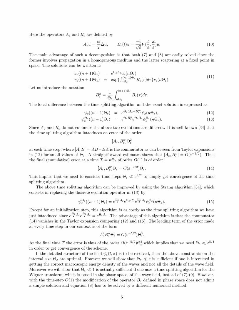
Here the operators Aε and Bε are defined by
Aεu =iε
2∆u, Bε(t)u =
−i√εV (
t
ε,xε)u. (10)
The main advantage of such a decomposition is that both (7) and (8) are easily solved since theformer involves propagation in a homogeneous medium and the latter scattering at a fixed point inspace. The solutions can be written as
uε((n+ 1)Θε) = eΘεAεuε(nΘε)vε((n+ 1)Θε) = exp{
∫ (n+1)Θε
nΘεBε(τ)dτ}vε(nΘε).
(11)
Let us introduce the notation
Bnε =
1Θε
∫ (n+1)Θε
nΘε
Bε(τ)dτ.
The local difference between the time splitting algorithm and the exact solution is expressed as
ψε((n+ 1)Θε) = eΘε(Aε+Bnε )ψε(nΘε), (12)
ψΘεε ((n+ 1)Θε) = eΘεBn
ε eΘεAεψΘεε (nΘε). (13)
Since Aε and Bε do not commute the above two evolutions are different. It is well known [34] thatthe time splitting algorithm introduces an error of the order
[Aε, Bnε ]Θ2
ε
at each time step, where [A,B] = AB−BA is the commutator as can be seen from Taylor expansionsin (12) for small values of Θε. A straightforward estimates shows that [Aε, B
nε ] = O(ε−3/2). Thus
the final (cumulative) error at a time T = nΘε of order O(1) is of order
[Aε, Bnε ]Θε = O(ε−3/2)Θε. (14)
This implies that we need to consider time steps Θε � ε3/2 to simply get convergence of the timesplitting algorithm.
The above time splitting algorithm can be improved by using the Strang algorithm [34], whichconsists in replacing the discrete evolution operator in (13) by
ψΘεε ((n+ 1)Θε) = e
Θε2
AεeΘεBnε e
Θε2
AεψΘεε (nΘε). (15)
Except for an initialization step, this algorithm is as costly as the time splitting algorithm we havejust introduced since e
Θε2
AεeΘε2
Aε = eΘεAε . The advantage of this algorithm is that the commutator(14) vanishes in the Taylor expansion comparing (12) and (15). The leading term of the error madeat every time step in our context is of the form
A2εB
nε Θ3
ε = O(ε−5/2)Θ3ε.
At the final time T the error is thus of the order O(ε−5/2)Θ2ε which implies that we need Θε � ε5/4
in order to get convergence of the scheme.If the detailed structure of the field ψε(t,x) is to be resolved, then the above constraints on the
interval size Θε are optimal. However we will show that Θε � ε is sufficient if one is interested ingetting the correct macroscopic energy density of the waves and not all the details of the wave field.Moreover we will show that Θε � 1 is actually sufficient if one uses a time splitting algorithm for theWigner transform, which is posed in the phase space, of the wave field, instead of (7)-(9). However,with the time-step O(1) the modification of the operator Bε defined in phase space does not admita simple solution and equation (8) has to be solved by a different numerical method.
5

3 Phase space energy and formal high frequency limit
We now describe what we mean by macroscopic energy density of waves and how we can computeit numerically. The dynamics of high frequency waves propagating in slowly varying media can beapproximated by WKB type expansions of the form
ψε(t,x) = A(t,x)eiS(t,x)/ε +O(ε), (16)
where the phase S and amplitude A are obtained by solving an eikonal and a transport equation,respectively [23]. In practice, the ansatz (16) is often sufficient for an accurate description of thewave field. A natural question is then to understand the size of Θε in the time splitting algorithmthat ensures that A and S are well approximated by the algorithm instead of the full wave field ψε.
However, the above expansion (16) is essentially useless in random media. The reason is that thewave field cannot be represented by one generalized plane wave of the form (16). Instead an infinitenumber of them is required because of multiple scattering. The theory of Wigner transforms in thephase space is a convenient way to overcome this difficulty and resolve the wave energy locally overall possible directions. The Wigner transform is defined as follows
Wε(t,x,k) =∫
Rd
eik·yψε(t,x−εy2
)ψ∗ε(t,x +εy2
)dy
(2π)d. (17)
Here ∗ denotes complex conjugation. The Wigner transform is thus the Fourier transform of thetwo-point correlation function of the field ψε. It roughly describes the energy density of waves attime t and position x propagating with wave vector k/ε.
Wigner transforms have been used intensively in recent years to understand high frequency wavepropagation in highly oscillatory periodic and random media [2, 18, 24, 30]. The spatial energydensity (probability density for quantum waves) is the integral of the Wigner transform over thewave vectors:
|ψε|2(t,x) =∫
Rd
Wε(t,x,k)dk. (18)
Our objective is therefore to understand how we can capture the main features of the Wignertransform (17) and then recover the physical space energy via (18). More precisely we want toobtain the critical size of Θε so that the statistical ensemble average E {Wε} (t,x,k) has the correctlimit as ε → 0. This allows us to describe the statistics of the spatial energy density withoutcapturing the detailed structure of ψε.
The rigorous analysis of the Wigner transform (17) of wave fields ψε that satisfy (6) has beenperformed in [3, 4] using the martingale technique under the assumption that V is a mean zerospatially homogeneous random potential with a two-point correlation function R(t,x):
E {V (t,x)} = 0, E {V (t,x)V (t+ s,x + y)} = R(s,y). (19)
It has been shown that in the limit ε → 0 the Wigner transform converges in probability to thesolution of the radiative transport equation
∂W
∂t+ k · ∇xW =
∫Rd
R(|p|2 − |k|2
2,p− k)(W (t,x,p)− W (t,x,k))
dp(2π)d
. (20)
Here R, the Fourier transform of the two-point correlation function, is the power spectrum of therandom process V . We extend this analysis to the case of discretized equations in time in Section 4.The main result is that with the time-step Θε = Θε the Wigner transform W ε
Θ of the solution of the
6

time-splitting scheme (7)-(9) converges as ε→ 0 to the solution of a radiative transport equation ofthe form
∂WΘ
∂t+ k · ∇xW
Θ =∫
Rd
RΘ(k,p)(WΘ(t,x,p)− WΘ(t,x,k))dp
(2π)d. (21)
The new scattering kernel RΘ(k,p) is given by (46) below. Before proceeding with a rigorous proof,we present in the rest of this section a formal but shorter path to the answer.
3.1 Radiative Transfer equation in the continuous case
First we formally derive the radiative transfer equation obtained in [3, 4] that Wε satisfies in thelimit ε→ 0. This is helpful in the understanding of the formal analysis of the semi-classical limit ofthe Wigner transform of the solution of the time-splitting scheme (7)-(9) presented in Section 3.2.
We recall that the Wigner transform (17) solves the following equation [4, 30]
∂Wε
∂t+ k · ∇xWε =
1i√ε
∫Rd
eip·x/εV (t
ε,p)
[W
(k− p
2
)−W
(k +
p2
)] dp(2π)d
. (22)
Here and in the sequel we denote the Fourier transform only in space by
f(t,p) =∫
Rd
e−ip·xf(t,x)dx, (23)
and the Fourier transform both in t and x by
f(t,p) =∫
Rd+1
e−iωt−ip·xf(t,x)dtdx. (24)
Equation (22) may be recast as
∂Wε
∂t+ k · ∇xWε =
∫Rd
Kε(t,x,k− p)Wε(t,x,p)dp, (25)
where Kε is given by
Kε(t,x,q) =1
iπd√ε
[V (
t
ε, 2q)ei2q·x/ε − V (
t
ε,−2q)e−i2q·x/ε
]. (26)
Inverting the free transport operator ∂t + k · ∇x we recast (25) as an integral equation
Wε(τ,x,k) = Wε(0,x− τk,k) +∫ τ
0
∫Kε(τ − s,x− sk,k− p)Wε(τ − s,x− sk,p)dpds. (27)
One more iteration yields
Wε(τ,x,k) = Wε(0,x− τk,k) +∫ τ
0
∫Kε(τ − s,x− sk,k− p)Wε(0,x− sk− (τ − s)p,p)dpds
+∫ τ
0
∫Kε(τ − s,x− sk,k− p)
∫ τ−s
0
∫Kε(τ − s− u,x− sk− up,p− q) (28)
×Wε(τ − s− u,x− sk− up,q)dqdudpds.
Let us now consider ensemble averaging in the above equation. We assume that the initial conditionWε(t = 0) is deterministic and that the potential V has mean zero. This implies that the secondterm on the right-hand side of (28) vanishes after ensemble averaging. To deal with the third term
7

we assume that Wε is statistically independent of the rest of the term. This step cannot be justifiedat this stage but it does provide the correct answer in the limit ε→ 0. By doing so we obtain that
E {Wε} (τ,x,k) = Wε(0,x− τk,k)
+∫ τ
0
∫ τ−s
0
∫R2d
E {Kε(τ − s,x− sk,k− p)Kε(τ − s− u,x− sk− up,p− q)}
×E {Wε} (τ − s− u,x− sk− up,q)dqdudpds.
(29)
We now have to compute the ensemble average of the product of two functions Kε. Taking theFourier transform of (19) in x → p yields
E{V (t,p)V (t+ s,q)
}= (2π)dR(s,p)δ(p + q). (30)
Straightforward algebra shows that
E {Kε(t,y,k− p)Kε(t− u,y − up,p− q)} (31)
=1πdε
R(u
ε, 2(p− k))
(e2iu(k−p)·p/ε + e−2iu(k−p)·p/ε
)(δ(k + q− 2p)− δ(k− q)).
Thus the ensemble average of the last term in (29) becomes∫ τ
0
∫ τ−s
0
∫Rd
R(u
ε, 2(p− k))
(e2iu(p−k)·p/ε + e−2iu(p−k)·p/ε
)×
(E {Wε} (τ − s− u,x− sk− up, 2p− k)− E {Wε} (τ − s− u,x− sk− up,k)
)dpdudsπdε
.
After the change of variables 2p− k → p and u→ εu, we get∫ τ
0
∫ (τ−s)/ε
0
∫Rd
dpduds(2π)d
R(u,p− k)(eiu
|p|2−|k|22 + e−iu
|p|2−|k|22
)(32)
×(E {Wε} (τ − s− εu,x− sk− εu
p + k2
,p)− E {Wε} (τ − s− εu,x− sk− εup + k
2,k)
).
Assuming that Wε is smooth in the limit ε→ 0 we thus obtain that (32) in the limit ε→ 0 yields∫ τ
0
∫Rd
R(|p|2 − |k|2
2,p− k)(E {W} (τ − s,x− sk,p)− E {W} (τ − s,x− sk,k))
dpds(2π)d
, (33)
where R(ω,p) is the power spectrum of the random potential V
R(ω,p) =∫ ∞
−∞e−iωuR(p, u)du. (34)
We replace the right side of (29) by (33) and obtain the integral equation for W , the limit of E {Wε}as ε→ 0:
W (τ,x,k) = W (0,x− τk,k) (35)
+∫ τ
0
∫Rd
R(|p|2 − |k|2
2,p− k)(W (τ − s,x− sk,p)−W (τ − s,x− sk,k))
dpds(2π)d
.
Equation (35) is nothing but the integral form of the transport equation (20). We thus obtain thatin the high frequency limit (as ε → 0) the average wave energy density is given by the solution tothe macroscopic equation (20) that no longer involves the small parameter ε.
8
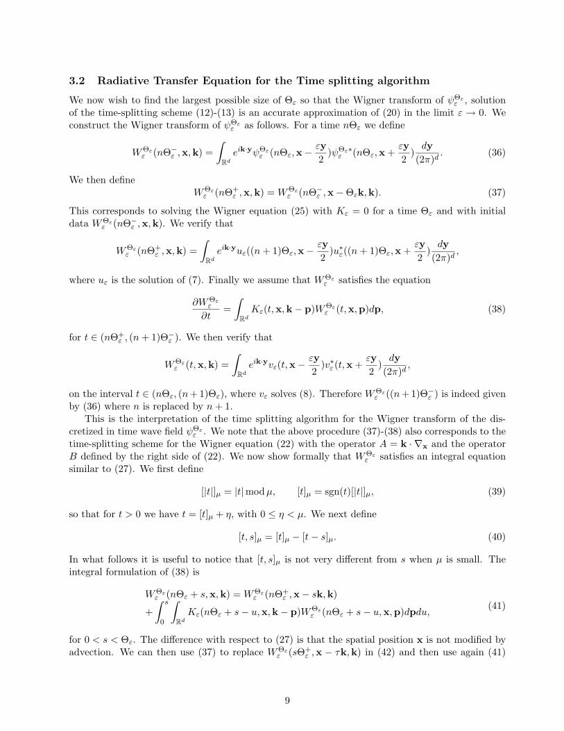
3.2 Radiative Transfer Equation for the Time splitting algorithm
We now wish to find the largest possible size of Θε so that the Wigner transform of ψΘεε , solution
of the time-splitting scheme (12)-(13) is an accurate approximation of (20) in the limit ε → 0. Weconstruct the Wigner transform of ψΘε
ε as follows. For a time nΘε we define
WΘεε (nΘ−
ε ,x,k) =∫
Rd
eik·yψΘεε (nΘε,x−
εy2
)ψΘε∗ε (nΘε,x +
εy2
)dy
(2π)d. (36)
We then defineWΘε
ε (nΘ+ε ,x,k) = WΘε
ε (nΘ−ε ,x−Θεk,k). (37)
This corresponds to solving the Wigner equation (25) with Kε = 0 for a time Θε and with initialdata WΘε
ε (nΘ−ε ,x,k). We verify that
WΘεε (nΘ+
ε ,x,k) =∫
Rd
eik·yuε((n+ 1)Θε,x−εy2
)u∗ε((n+ 1)Θε,x +εy2
)dy
(2π)d,
where uε is the solution of (7). Finally we assume that WΘεε satisfies the equation
∂WΘεε
∂t=
∫Rd
Kε(t,x,k− p)WΘεε (t,x,p)dp, (38)
for t ∈ (nΘ+ε , (n+ 1)Θ−
ε ). We then verify that
WΘεε (t,x,k) =
∫Rd
eik·yvε(t,x−εy2
)v∗ε(t,x +εy2
)dy
(2π)d,
on the interval t ∈ (nΘε, (n+ 1)Θε), where vε solves (8). Therefore WΘεε ((n+ 1)Θ−
ε ) is indeed givenby (36) where n is replaced by n+ 1.
This is the interpretation of the time splitting algorithm for the Wigner transform of the dis-cretized in time wave field ψΘε
ε . We note that the above procedure (37)-(38) also corresponds to thetime-splitting scheme for the Wigner equation (22) with the operator A = k · ∇x and the operatorB defined by the right side of (22). We now show formally that WΘε
ε satisfies an integral equationsimilar to (27). We first define
[|t|]µ = |t|modµ, [t]µ = sgn(t)[|t|]µ, (39)
so that for t > 0 we have t = [t]µ + η, with 0 ≤ η < µ. We next define
[t, s]µ = [t]µ − [t− s]µ. (40)
In what follows it is useful to notice that [t, s]µ is not very different from s when µ is small. Theintegral formulation of (38) is
WΘεε (nΘε + s,x,k) = WΘε
ε (nΘ+ε ,x− sk,k)
+∫ s
0
∫Rd
Kε(nΘε + s− u,x,k− p)WΘεε (nΘε + s− u,x,p)dpdu,
(41)
for 0 < s < Θε. The difference with respect to (27) is that the spatial position x is not modified byadvection. We can then use (37) to replace WΘε
ε (sΘ+ε ,x − τk,k) in (42) and then use again (41)
9

on the interval ((n − 1)Θε, nΘε) and keep repeating the same process downwards until time t = 0.This yields
WΘεε (τ,x,k) = WΘε
ε (0+,x− [τ ]Θεk,k)
+∫ τ
0ds
∫Rd
dpKε(τ − s,x− [τ, s]Θεk,k− p)WΘεε (τ − s,x− [τ, s]Θεk,p).
(42)
We can replace WΘεε in the integral term above by its expression in (42) and then take ensemble
average of all terms in the equation. With the same assumptions that led to (29) we get
E{WΘε
ε
}(τ,x,k) = WΘε
ε (0+,x− τk,k)
+∫ τ
0
∫ τ−s
0
∫R2d
E {Kε(τ − s,x− [τ, s]Θεk,k− p)
× Kε(τ − s− u,x− [τ, s]Θεk− [τ − s, u]Θεp,p− q)}×E
{WΘε
ε
}(τ − s− u,x− [τ, s]Θεk− [τ − s, u]Θεp,q)dqdudpds.
(43)
Following the same calculations as in the continuous case we deduce that the second term on theright-hand side in the above equation is given by∫ τ
0
∫ τ−s
0
∫Rd
dpduds(2π)d
1εR(u
ε,p− k)
(ei[τ−s,u]Θε
|p|2−|k|22ε + e−i[τ−s,u]Θε
|p|2−|k|22ε
)×
(E
{WΘε
ε
}(τ − [τ, s]Θε − [τ − s, u]Θε ,x− [τ, s]Θεk− [τ − s, u]Θεp,p)
−E{WΘε
ε
}(τ − [τ, s]Θε − [τ − s, u]Θε ,x− [τ, s]Θεk− [τ − s, u]Θεp,k)
).
(44)
Let us assume that Θε = εΘ and that WΘεε has a smooth limit so it does not oscillate at the ε scale.
Moreover we realize that as ε → 0, [τ, s]Θε → s and change variables u/ε → u. This allows us toobtain that (44) in the limit ε→ 0 converges to∫ τ
0
∫Rd
dpRΘ(k,p)(WΘ(τ − s,x− sk,k)−WΘ(τ − s,x− sk,p))dp, (45)
where the power spectrum RΘ is given by
RΘ(k,p) =∫ ∞
0du
1Θ
∫ Θ
0dτR(u,p− k)
(ei[u+τ ]Θ
|p|2−|k|22 + e−i[u+τ ]Θ
|p|2−|k|22
). (46)
We insert (45) into the right side of (43) and obtain in the limit ε→ 0 that E{WΘε
ε
}converges to
WΘ, solution of
WΘ(τ,x,k) = WΘ(0,x− τk,k) (47)
+∫ τ
0
∫Rd
dpRΘ(k,p)(WΘ(τ − s,x− sk,k)− WΘ(τ − s,x− sk,p))dp.
This is the integral form of the radiative transport equation
∂WΘ
∂t+ k · ∇xW
Θ =∫
Rd
RΘ(k,p)[WΘ(t,x,p)− WΘ(t,x,k)]dp
(2π)d. (48)
This equation is nothing but (20) with the exact power spectrum R replaced by its modification RΘ.Therefore WΘε
ε will have the correct limit E {W} provided that the power spectrum RΘ is a goodapproximation of R. It is not difficult to check that
RΘ(k,p) = R(|p|2 − |k|2
2,p− k) +O(Θ) (49)
10

as Θ → 0 since [u+ τ ]Θ = u+O(Θ). Therefore in this limit we recover the correct power spectrum,as in the radiative transport equation (20). The other limit Θ → ∞ is also quite interesting. Onefinds that
RΘ(k,p) = R(0,p− k) +O(1Θ
). (50)
The scaling Θε = εΘ thus completely characterizes the quality of the time splitting discretizationas far as getting the correct macroscopic energy limit is concerned. When Θε � ε we obtain thecorrect energy limit with an error of order Θεε
−1. When Θε ∼ ε we get a transport equation withthe wrong power spectrum. When Θε � ε we also obtain a transport equation in the limit but witha white noise power spectrum. Indeed the power spectrum R(0,p− k) is the Fourier transform of atwo point correlation function
E {V (t,x)V (t+ s,x + y)} = R(y)δ(s),
which means that potentials at different times are totally uncorrelated. This result does not cometotally as a surprise. In the time splitting algorithm averaging occurs at one spatial position in (8)since advection is shut off. When the interval over which this averaging takes place is long, correla-tions with other parts of the system are lost and one converges to a power spectrum correspondingto fluctuations with full decorrelation in time.
4 The high-frequency limit of the time-splitting scheme
In this section we analyze rigorously the passage to the limit ε → 0 in the time-splitting scheme(7)-(9). The analysis is performed in the framework of the time-splitting scheme (37)-(38) for theWigner equation that is induced by (7)-(9). In particular we justify the modified radiative equation(48) in the small ε limit.
The method of proof is based on the ideas of [3] and [4]. In those works two types of convergencesare considered depending on the a priori bounds the Wigner transform W (t,x,k) satisfies. For theWigner transform of a pure state such as defined by (17) the a priori bound is in A′(R2d) uniformlyin time, where A′(R2d) is a distribution space bigger than the space of bounded measures [3, 24].We can also assume that the initial data for the Wigner transform has a strong limit in the smallerspace L2(R2d), which implies an a priori bound in the same space uniformly in time for the Wignertransform. Such a bound can be obtained by considering a mixture of states, which correspondsto taking the initial data ψε for the Schrodinger equation random and suitably averaging over thisrandomness first. The L2 setting also appears naturally in the mathematical theory of time reversalexperiments (see [3, 4] for details and our conclusions section).
In this section we assume the latter L2 a priori bound for two reasons. First the proofs are simplerin this setting and second we show that not only does the average Wigner transform converge tothe solution of (48), but it actually converges to its deterministic limit in probability. This meansthat it is a self-averaging quantity essentially independent of the realization of the random medium.This important property in time reversal applications has received some attention recently [1, 4, 28].When the main object of interest is evolution of a pure state then the limit Wigner transform doesnot belong to L2. Theorem 4.1 below still holds but only in the sense that the expectation of theWigner transform converges to the solution of (48). The proof is similar to what we present belowwith modifications as in [3].
4.1 Assumptions on the random potential
We begin with the assumptions on the random potential V (t,x). We assume that the random fieldV (t,x) is a Markov process in t, as in [3, 4]. The Markovian hypothesis is crucial to simplify the
11
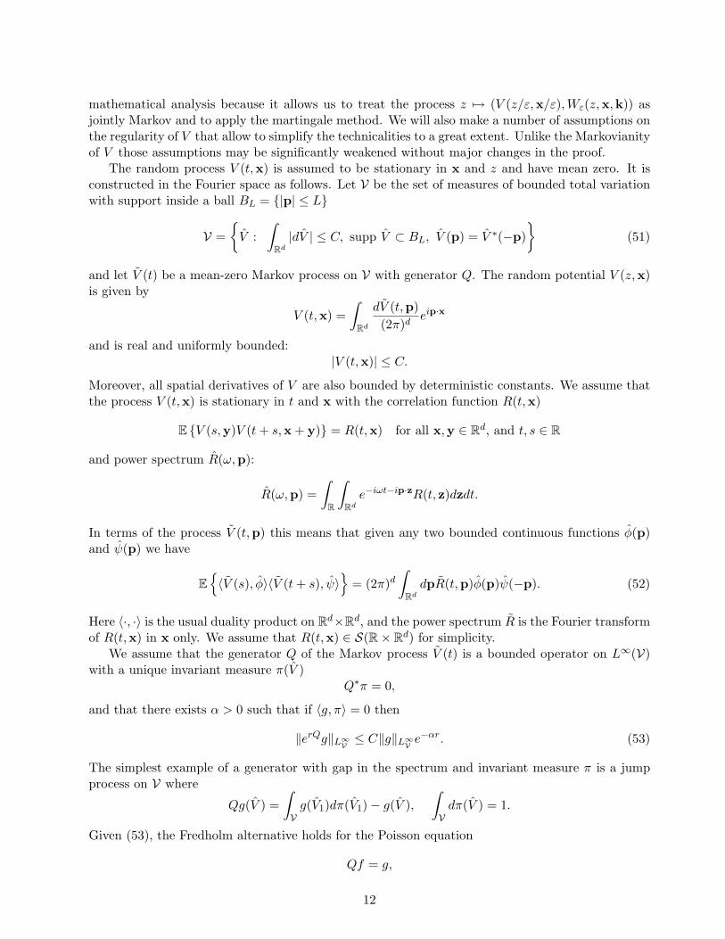
mathematical analysis because it allows us to treat the process z 7→ (V (z/ε,x/ε),Wε(z,x,k)) asjointly Markov and to apply the martingale method. We will also make a number of assumptions onthe regularity of V that allow to simplify the technicalities to a great extent. Unlike the Markovianityof V those assumptions may be significantly weakened without major changes in the proof.
The random process V (t,x) is assumed to be stationary in x and z and have mean zero. It isconstructed in the Fourier space as follows. Let V be the set of measures of bounded total variationwith support inside a ball BL = {|p| ≤ L}
V ={V :
∫Rd
|dV | ≤ C, supp V ⊂ BL, V (p) = V ∗(−p)}
(51)
and let V (t) be a mean-zero Markov process on V with generator Q. The random potential V (z,x)is given by
V (t,x) =∫
Rd
dV (t,p)(2π)d
eip·x
and is real and uniformly bounded:|V (t,x)| ≤ C.
Moreover, all spatial derivatives of V are also bounded by deterministic constants. We assume thatthe process V (t,x) is stationary in t and x with the correlation function R(t,x)
E {V (s,y)V (t+ s,x + y)} = R(t,x) for all x,y ∈ Rd, and t, s ∈ R
and power spectrum R(ω,p):
R(ω,p) =∫
R
∫Rd
e−iωt−ip·zR(t, z)dzdt.
In terms of the process V (t,p) this means that given any two bounded continuous functions φ(p)and ψ(p) we have
E{〈V (s), φ〉〈V (t+ s), ψ〉
}= (2π)d
∫Rd
dpR(t,p)φ(p)ψ(−p). (52)
Here 〈·, ·〉 is the usual duality product on Rd×Rd, and the power spectrum R is the Fourier transformof R(t,x) in x only. We assume that R(t,x) ∈ S(R× Rd) for simplicity.
We assume that the generator Q of the Markov process V (t) is a bounded operator on L∞(V)with a unique invariant measure π(V )
Q∗π = 0,
and that there exists α > 0 such that if 〈g, π〉 = 0 then
‖erQg‖L∞V≤ C‖g‖L∞V
e−αr. (53)
The simplest example of a generator with gap in the spectrum and invariant measure π is a jumpprocess on V where
Qg(V ) =∫Vg(V1)dπ(V1)− g(V ),
∫Vdπ(V ) = 1.
Given (53), the Fredholm alternative holds for the Poisson equation
Qf = g,
12
provided that g satisfies 〈π, g〉 = 0. It has a unique solution f with 〈π, f〉 = 0 and ‖f‖L∞V≤ C‖g‖L∞V
.The solution f is given explicitly by
f(V ) = −∫ ∞
0erQg(V )dr,
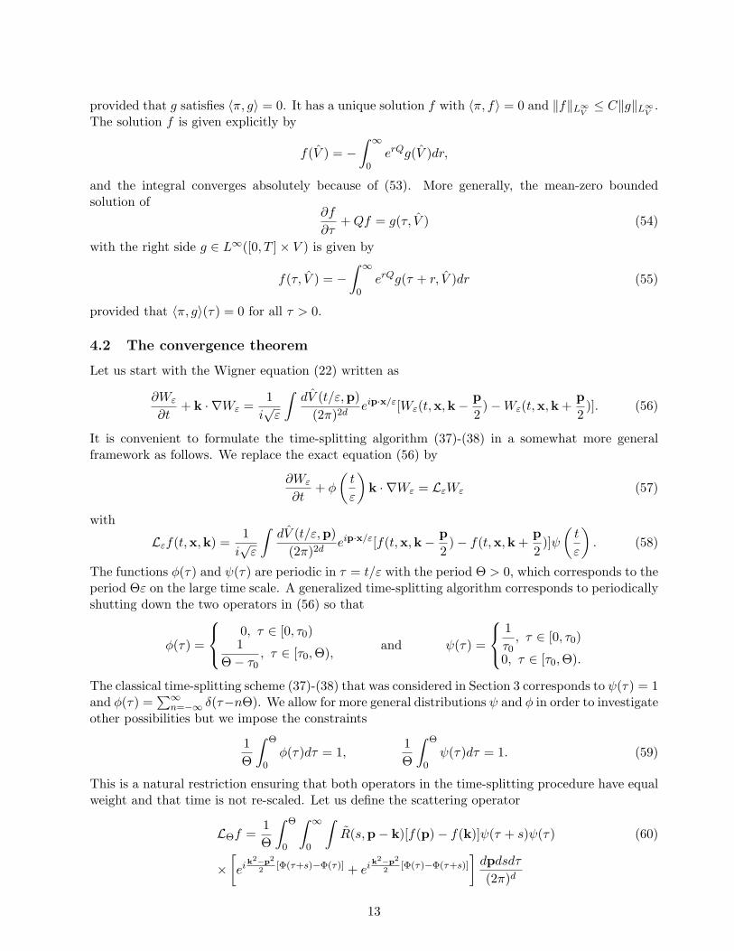
and the integral converges absolutely because of (53). More generally, the mean-zero boundedsolution of
∂f
∂τ+Qf = g(τ, V ) (54)
with the right side g ∈ L∞([0, T ]× V ) is given by
f(τ, V ) = −∫ ∞
0erQg(τ + r, V )dr (55)
provided that 〈π, g〉(τ) = 0 for all τ > 0.
4.2 The convergence theorem
Let us start with the Wigner equation (22) written as
∂Wε
∂t+ k · ∇Wε =
1i√ε
∫dV (t/ε,p)
(2π)2deip·x/ε[Wε(t,x,k−
p2
)−Wε(t,x,k +p2
)]. (56)
It is convenient to formulate the time-splitting algorithm (37)-(38) in a somewhat more generalframework as follows. We replace the exact equation (56) by
∂Wε
∂t+ φ
(t
ε
)k · ∇Wε = LεWε (57)
with
Lεf(t,x,k) =1i√ε
∫dV (t/ε,p)
(2π)2deip·x/ε[f(t,x,k− p
2)− f(t,x,k +
p2
)]ψ(t
ε
). (58)
The functions φ(τ) and ψ(τ) are periodic in τ = t/ε with the period Θ > 0, which corresponds to theperiod Θε on the large time scale. A generalized time-splitting algorithm corresponds to periodicallyshutting down the two operators in (56) so that
φ(τ) =
0, τ ∈ [0, τ0)1
Θ− τ0, τ ∈ [τ0,Θ),
and ψ(τ) =
1τ0, τ ∈ [0, τ0)
0, τ ∈ [τ0,Θ).
The classical time-splitting scheme (37)-(38) that was considered in Section 3 corresponds to ψ(τ) = 1and φ(τ) =
∑∞n=−∞ δ(τ−nΘ). We allow for more general distributions ψ and φ in order to investigate
other possibilities but we impose the constraints
1Θ
∫ Θ
0φ(τ)dτ = 1,
1Θ
∫ Θ
0ψ(τ)dτ = 1. (59)
This is a natural restriction ensuring that both operators in the time-splitting procedure have equalweight and that time is not re-scaled. Let us define the scattering operator
LΘf =1Θ
∫ Θ
0
∫ ∞
0
∫R(s,p− k)[f(p)− f(k)]ψ(τ + s)ψ(τ) (60)
×[ei
k2−p2
2[Φ(τ+s)−Φ(τ)] + ei
k2−p2
2[Φ(τ)−Φ(τ+s)]
]dpdsdτ(2π)d
13

where Φ(s) is an anti-derivative of φ:dΦdτ
= φ. Since only increments of Φ appear in our results thechoice of a particular anti-derivative is irrelevant. The main result of this section is the followingtheorem.
Theorem 4.1 Let the initial data W 0ε (x,k) for (57) converge to W0(x,k) strongly in L2(R2d). Then
the modified Wigner distribution Wε, solution of (57) converges in probability and weakly in L2(Rd)to the solution W of the modified transport equation
∂W
∂t+ k · ∇W = LΘW (61)
with the initial data W0(x,k). More precisely, for any test function λ ∈ L2(Rd) the random process
〈W,λ(t)〉 =∫
R2d
Wε(t,x,k)λ(x,k)dxdk
converges in probability to 〈W,λ〉 as ε→ 0 uniformly on finite time intervals t ∈ [0, T ].
It is instructive to consider two limiting cases: Θ → 0 and Θ → ∞ as in the discussion at theend of Section 3. The first case corresponds to time splitting with a very small time step, whenwe expect a very good approximation to the true statistics. The second arises when the time stepis very large and the oscillatory random potential has large variations inside each time step. Thenwe expect that such variations would appear as white noise. Indeed, we replace for convenienceψ → ψ(τ/Θ) and φ→ φ(τ/Θ) and observe as Θ →∞
LΘf =1Θ
∫ Θ
0
∫ ∞
0
∫R(s,p− k)[f(p)− f(k)]ψ
(τ + s
Θ
)ψ
( τΘ
)×
[ei
k2−p2
2[Φ( τ+s
Θ )−Φ( τΘ)] + ei
k2−p2
2[Φ( τ
Θ)−Φ( τ+sΘ )]
]dpdsdτ(2π)d
=∫ 1
0
∫ ∞
0
∫R(s,p− k)[f(p)− f(k)]ψ
(τ +
s
Θ
)ψ (τ)
×[ei
k2−p2
2[Φ(τ+ s
Θ)−Φ(τ)] + eik2−p2
2[Φ(τ)−Φ(τ+ s
Θ)]]dpdsdτ(2π)d
→(∫ 1
0|ψ(τ)|2dτ
) ∫R(0,p− k)[f(p)− f(k)]
dp(2π)d
.
It is interesting to observe that in the limit Θ → ∞ the scattering operator does not depend onthe choice of the function φ at all, so that advection may be carried out in any fashion. The onlydependence on the function ψ is that it controls the magnification of the scattering operator viaits L2-norm. Moreover, the scattering kernel coincides with that in (50). As we have discussedpreviously the kernel R(ω,p) that is independent of ω corresponds to the white noise limit in time.However, even in the white noise regime the correct amplification factor is obtained only if ‖ψ‖L2 = 1which together with (59) implies that ψ = 1. This means that in order to capture the correct limitin the white noise scaling one has to keep the scattering “switched on” at all times. Otherwiseinformation is lost which leads to an incorrect limit.
In the opposite limit Θ → 0 the function Φ(s) may be decomposed as
Φ(s) =∫ s
0φ
(ξ
Θ
)dξ = s+ Θ
∫ s/Θ−[s/Θ]
0(φ(ξ)− 1) dξ = s+ ΘΦ
( sΘ
),
14

where [s] is the integer part of s. The function Φ is periodic in Θ and bounded so that Φ(s) → s asΘ → 0. The same change of variables as in the case Θ →∞ shows that
LΘf →∫ 1
0dτ
∫ 1
0dζ
∫ ∞
0ds
∫dp
(2π)dR(s,p− k)[f(p)− f(k)]ψ(τ + ζ)ψ (τ)
×[ei
k2−p2
2s + e−ik
2−p2
2s
]=
∫dp
(2π)dR
(p2 − k2
2,p− k
)[f(p)− f(k)].
We see that the correct power spectrum is recovered in this limit. Therefore the time-splittingscheme (57) has the correct behavior for an arbitrary choice of the controls φ and ψ that satisfy (59)provided that the time step Θε = Θε with Θ � 1, or equivalently Θε � ε.
Another important special case arises when ψ = 1 and φ(τ) = Θ∑∞
j=−∞ δ(τ − jΘ). Thiscorresponds to the time-splitting scheme (37)-(38) when scattering is accounted for at all times whileadvection is accounted for at times t = jεΘ by the correction W (εjΘ+,x,k) = W (εjΘ−,x−εΘk,k).This is exactly the algorithm analyzed formally in Section 3. Then we have Φ(s) = Θ[s/Θ] := [s]Θand obtain the following expression for LΘ:
LΘf =1Θ
∫ Θ
0
∫ ∞
0
∫R(s,p− k)[f(p)− f(k)]
×[ei
k2−p2
2([τ+s]Θ−[τ ]Θ) + ei
k2−p2
2([τ ]Θ−[τ+s]Θ)
]dpds(2π)d
.
However, we have [τ ]Θ = 0 when 0 ≤ τ < Θ and we obtain
LΘf =1Θ
∫ Θ
0
∫ ∞
0
∫R(s,p− k)[f(p)− f(k)]
[ei
k2−p2
2[τ+s]Θ + e−ik
2−p2
2[τ+s]Θ
]dpds(2π)d
. (62)
The operator LΘ in (62) coincides with that obtained in (46) by the formal calculation and hencethe limit equation (61) is nothing but (48) in this case.
4.3 Outline of the proof
The proof of Theorem 4.1 follows the idea of the proof of the main result in [4]. Therefore we outlinethe main steps and concentrate only on the necessary modifications in the proof. First one mayshow that the family of measures Pε generated by the process Wε(t) on C([0, T ];L2(R2d)) is tight.
Lemma 4.2 The family of measures Pε is weakly compact.
The proof of this lemma is very similar to that in [4] and is omitted. It is straightforwardto verify that the L2-norm of Wε is preserved by evolution and hence Wε takes values in a ballX = {W ∈ L2 : ‖W‖L2 ≤ C}.
Lemma 4.3 The L2-norm of the modified Wigner distribution is preserved:
‖Wε(t)‖L2(R2d) = ‖Wε(0)‖L2(R2d). (63)
Let λ(t,x,k) be a fixed deterministic function. In order to identify the limit of Wε we constructa functional Gλ : C([0, T ];X) → C[0, T ] defined by
Gλ[W ](t) = 〈W,λ〉(t)−∫ t
0〈W, ∂λ
∂t+ k · ∇xλ+ LΘλ〉(s)ds (64)
and show that it is an approximate martingale. More precisely, we show that the following lemmaholds.
15

Lemma 4.4 There exists a constant C > 0 so that∣∣EPε {Gλ[W ](t)|Fs} −Gλ[W ](s)∣∣ ≤ Cλ,T
√ε (65)
uniformly for all W ∈ C([0, T ];X) and 0 ≤ s < t ≤ T .
The proof of Lemma 4.4 is based on the construction of an exact martingale Gελ[W ] that is
uniformly close to Gλ[W ] within O(√ε). Lemma 4.2 implies that there exists a subsequence εj → 0
so that Pεj converges weakly to a measure P supported on C([0, T ];X). Weak convergence of Pε
and the strong convergence (65) together imply that Gλ[W ](t) is a P -martingale so that
EP {Gλ[W ](t)|Fs} −Gλ[W ](s) = 0. (66)
Taking s = 0 above we obtain as in [3] the transport equation (61) for W = EP {W (t)} in its weakformulation. Construction of the martingale Gε
λ and the proof of Lemma 4.4 are presented in detailin Section 4.4.
The second step is to show that for every test function λ(t,x,k) the new functional
G2,λ[W ](t) = 〈W,λ〉2(t)− 2∫ t
0〈W,λ〉(s)〈W, ∂λ
∂s+ k · ∇xλ+ LΘλ〉(s)ds
is also an approximate Pε-martingale. We then obtain that EPε{〈W,λ〉2
}→ 〈W,λ〉2, which implies
convergence in probability. It follows that the limit measure P is unique and deterministic, and thatthe whole sequence Pε converges. All the modifications required in this step compared to [4] arevery similar to those in the proof of Lemma 4.4 in the construction of the martingale Gε
λ and we donot present the details in this part of the proof.
4.4 The approximate martingale
To obtain the approximate martingale property (65) and prove Lemma 4.4, one has to consider theconditional expectation of functionals F (W, V ) with respect to the probability measure Pε on thespace C([0, T ];V × X) generated by V (t/ε) and the Cauchy problem (57). The only functions weneed to consider are actually of the form F (W, V ) = 〈W,λ(V )〉 with λ ∈ L∞(V;C1([0, T ];S(R2d))).Given a function F (W, V ) let us define the conditional expectation
EPε
W,V ,t
{F (W, V )
}(τ) = EPε
{F (W (τ), V (τ))| W (t) = W, V (t) = V
}, τ ≥ t.
The weak form of the infinitesimal generator of the Markov process generated by Pε is given by
d
dhEPε
W,V ,t
{〈W,λ(V )〉
}(t+ h)
∣∣∣∣h=0
=1ε〈W,Qλ〉+
⟨W,
(∂
∂t+ φ
(t
ε
)k · ∇x +
1√εK[V ,
t
ε,xε])λ
⟩,
(67)hence
Gελ = 〈W,λ(V )〉(t)−
∫ t
0
⟨W (s),
(1εQ+
∂
∂s+ φ
(sε
)k · ∇x +
1√εK[V ,
s
ε,xε])λ(s)
⟩ds (68)
is a Pε-martingale. The operator K is defined by
K[V , τ, z]f(x, τ, z,k, V ) =1i
∫Rd
dV (p)(2π)d
eip·z[f(τ,x, z,k− p
2)− f(τ,x, z,k +
p2
)]ψ(τ). (69)
16

The generator (67) comes from equation (57) written in the form
∂Wε
∂t+ φ
(t
ε
)k · ∇xWε =
1√εK[V (
t
ε),t
ε,xε]Wε. (70)
Given a test function λ(t,x,k) ∈ C1([0, L];S) we will construct a function
λε(t,x,k, V ) = λ(t,x,k) +√ελε
1(t,x,k, V ) + ελε2(t,x,k, V ) (71)
with the correctors λε1,2(t) bounded in L∞(V;L2(R2d)) uniformly in t ∈ [0, T ]. The functions λε
1,2
will be chosen so that‖Gε
λε(t)−Gλ(t)‖L∞(V) ≤ Cλ
√ε (72)
for all t ∈ [0, T ]. Here Gελε
is defined by (68) with λ replaced by λε, and Gλ is defined by (64). Theapproximate martingale property (65) follows from this.
The functions λε1 and λε
2 are defined as follows. Let λ1(t, τ,x, z,k, V ) be the mean-zero solutionof
∂λ1
∂τ+ φ(τ)k · ∇zλ1 +Qλ1 = −1
i
∫dV (p)(2π)d
eip·z[λ(x,k− p
2)− λ(x,k +
p2
)]ψ(τ), (73)
where V (p) is fixed and independent of τ . This equation has a form similar to (54) and its solutionis given by an appropriate modification of (55):
λ1(t, τ,x, z,k, V ) =1i
∫ ∞
0esQ
∫dV (p)(2π)d
ei(p·z+(k·p)[Φ(τ+s)−Φ(τ)])
×[λ(t,x,k− p
2)− λ(t,x,k +
p2
)]ψ(τ + s)ds. (74)
The equation for λ2 is
(∂τ + φ(τ)k · ∇z +Q)λ2 = LΘλ−Kλ1 + [1− φ(τ)]k · ∇xλ. (75)
The first term on the right may be recast as(LΘλ− Lτ
Θλ)
+(Lτ
Θλ−Kλ1
).
We decompose λ2 as λ21 + λ22 + λ23, corresponding to the arising three source terms, respectively.The operator LΘ is defined by (60) while Lτ
Θ is defined by
LτΘλ = E {Kλ1} .
Before proceeding with the solution for λ2 we find the explicit form of LτΘ and verify that
LΘλ =1Θ
∫ Θ
0Lτ
Θλdτ, (76)
where Θ is the period of φ and ψ. Let us first compute LτΘλ:
LτΘλ(t, τ,x, z,k) = −1
iE
{∫dV (p)(2π)d
eip·z[λ1
(t, τ,x, z,k− p
2
)− λ1
(t, τ,x, z,k +
p2
)]ψ(τ)
}= I + I∗.
17

We have
I = −1iE
{∫dV (p)(2π)d
eip·zλ1
(k +
p2
)ψ(τ)
}
= E
{∫dV (p)(2π)d
eip·z∫ ∞
0esQ
∫dV (q)(2π)d
ei((q·z)+((k+p/2)·q)[Φ(τ+s)−Φ(τ)])
}×
[λ(k +
p2− q
2)− λ(k +
p2
+q2)]ψ(τ + s)ψ(τ)ds
=∫ ∞
0
∫R(s,p)e−i(k+p/2)·p[Φ(τ+s)−Φ(τ)][λ(k + p)− λ(k)]ψ(τ + s)ψ(τ)
dpds(2π)d
=∫ ∞
0
∫R(s,p− k)ei(k
2−p2)[Φ(τ+s)−Φ(τ)]/2[λ(p)− λ(k)]ψ(τ + s))ψ(τ)dpds(2π)d
.
Then we obtain
LτΘλ(t, τ,x,k) =
∫ ∞
0
∫R(s,p− k)[λ(t,x,p)− λ(t,x,k)]
×[ei(k
2−p2)[Φ(τ+s)−Φ(τ)]/2 + ei(k2−p2)[Φ(τ)−Φ(τ+s)]/2
]ψ(τ + s)ψ(τ)
dpds(2π)d
(77)
and (76) follows. We observe that the operators LΘ and LτΘ are independent of V and z and therefore
the function λ21 = λ21(t, τ,x,k) is also independent of these variables. It is given explicitly by
λ21(t, τ,x,k) =∫ τ
0[LΘ(t,x,k)− Lτ
Θ(t, ζ,x,k)]λ(t,x,k)dζ (78)
and is periodic in the fast variable τ . Similarly the function λ23 is also independent of V and z andis given by
λ23(t, τ,x,k) = [τ − Φ(τ)]k · ∇xλ(t,x,k). (79)
The function λ22 satisfies
∂λ22
∂τ+ φ(τ)k · ∇zλ22 +Qλ22 = Lτ
Θλ−Kλ1.
It is given explicitly by
λ22(t, τ,x, z,k, V ) = −∫ ∞
0esQ[Lτ
Θλ(t, τ+s,x,k)−Kλ1(t, τ+s,x, z+(Φ(τ+s)−Φ(τ))k,k, V )]. (80)
Using (73) and (75) we have
d
dhEPε
W,V ,t{〈W,λε〉} (t+ h)
∣∣∣∣h=0
=⟨W,
(∂
∂t+ φ
(t
ε
)k · ∇x +
1√εK[V ,
t
ε,xε] +
1εQ
)(λ+
√ελε
1 + ελε2
)⟩=
⟨W,
(∂
∂t+ k · ∇x
)λ+ LΘλ
⟩+
⟨W,
(∂
∂t+ φ
(t
ε
)k · ∇x
) (√ελε
1 + ελε2
)+√εK[V ,
t
ε,xε]λε
2
⟩=
⟨W,
(∂
∂t+ k · ∇x
)λ+ LΘλ
⟩+√ε〈W, ζλ
ε 〉
18

with
ζλε =
(∂
∂t+ φ
(t
ε
)k · ∇x
)λε
1 +√ε
(∂
∂t+ φ
(t
ε
)k · ∇x
)λε
2 +K[V ,t
ε,xε]λε
2.
The terms k ·∇xλε1,2 above are understood as differentiation with respect to the slow variable x only,
and not with respect to z = x/ε. It follows that Gελε
is given by
Gελε
(t) = 〈W (t), λε〉 −∫ t
0
⟨W,
(∂
∂t+ k · ∇x + LΘ
)λ
⟩(s)ds−
√ε
∫ t
0〈W, ζλ
ε 〉(s)ds (81)
and is a martingale with respect to the measure Pε defined on C([0, T ];X ×V). Lemma 4.4 and theestimate (65) follow from the following two lemmas.
Lemma 4.5 Let λ ∈ C1([0, T ];S(R2d)). Then there exists a constant Cλ > 0 independent of t ∈[0, T ] so that the correctors λε
1(t) and λε2(t) satisfy the uniform bounds
‖λε1(t)‖L∞(V;L2) + ‖λε
2(t)‖L∞(V;L2) ≤ Cλ (82)
and ∥∥∥∂λε1(t)∂t
+ φ
(t
ε
)k · ∇xλ
ε1(t)
∥∥∥L∞(V;L2)
+∥∥∥∂λε
2(t)∂t
+ φ
(t
ε
)k · ∇xλ
ε2(t)
∥∥∥L∞(V;L2)
≤ Cλ. (83)
Lemma 4.6 There exists a constant Cλ such that
‖K[V , t/ε,x/ε]‖L2→L2 ≤ C
for any V ∈ V and all ε ∈ (0, 1].
Proof of lemma 4.4. Observe that (82) implies that |〈W,λ〉 − 〈W,λε〉| ≤ C√ε for all W ∈ X
and V ∈ V, while (83) and Lemma 4.6 imply that for all t ∈ [0, T ]
‖ζλε (t)‖L2 ≤ C (84)
for all V ∈ V so that (65) follows from the fact that (81) is a martingale.Proof of Lemma 4.6. Lemma 4.6 follows immediately from the definition of K, the uniform
bound on the total mass of V in (51) and the Cauchy-Schwartz inequality. We have Kf = I + I∗,with
I(x,k) =1i
∫Rd
dV (p)(2π)d
eip·x/εf(x,k− p2
)ψ(t
ε
)and ∫
|I(x,k)|2 =∫
R4d
ei(p−q)·x/εf(x,k− p2
)f(x,k− q2)∣∣∣∣ψ(
t
ε
)∣∣∣∣2 dV (p)dV (q)dxdk(2π)2d
≤ C
∫|dV (p)||dV (q)|
(2π)2d‖f‖2
L2 ≤ C‖f‖2L2 .
We now prove Lemma 4.5. We will omit the t-dependence of the test function λ to simplifynotation.
Proof of Lemma 4.5. We only prove (82). Since λ ∈ S(R2d), there exists a constant Cλ sothat
|λ(x,k)| ≤ Cλ
(1 + |x|5d)(1 + |k|5d).
19

Then we obtain using (51) and (53)
|λε1(t,x,k, V )| ≤ C
∣∣∣∣∫ ∞
0esQ
∫dV (p)ei(p·z+(k·p)[Φ(t/ε+s)−Φ(t/ε)])
[λ(k− p
2)− λ(k +
p2
)]∣∣∣∣
≤ C
∫ ∞
0dre−αr sup
V
∫Rd
|dV (p)|[|λ(z,x,k− p
2)|+ |λ(z,x,k +
p2
)|]
≤ C
(1 + |x|5d)(1 + (|k| − L)5dχ|k|≥5L(k))
and the L2-bound on λ1 follows. Here L is the size of the support of V as in (51).We show next that λε
2 is uniformly bounded. Recall that λε2 = λε
21 + λε22 + λε
23 with the threeterms given by (78), (80) and (79), respectively. The L2-bound on λ23 follows immediately from thefact that |τ − Φ(τ)| ≤ C because of (59). We also note that
λ21(t, τ,x,k) =∫ τ
nΘ[LΘ(t,x,k)− Lτ
Θ(t, ζ,x,k)]λ(t,x,k)dζ (85)
where nΘ ≤ τ < (n+ 1)Θ. Moreover, we note that for all τ > 0 we have
|(LτΘλ(t, τ,x,k)| ≤ C
∫Z(p− k)[|λ(t,x,p)|+ |λ(t,x,k)|]dp, (86)
where Z(k) =∫ ∞
0|R(s,k)| and hence ‖(Lτ
Θλ(t, τ,x,k)‖L2(R2d) ≤ Cλ for all t and τ . This in turn
implies that ‖(LΘλ)(t,x,k)‖L2 ≤ Cλ so that (85) implies that λε21 is uniformly bounded in L2. We
have for λ22:
λε22(t,x,k, V ) = −
∫ ∞
0dsesQ
{Lτ
Θλ(t,t
ε+ s,x,k)− 1
i
∫Rd
dV (p)(2π)d
eip·(x/ε+(Φ(t/ε+s)−Φ(t/ε))k)
×[λ1(t,
t
ε+ s,x,
xε
+ (Φ(t
ε+ s)− Φ(
t
ε))k,k− p
2, V )
−λ1(t,t
ε+ s,x,
xε
+ (Φ(t
ε+ s)− Φ(
t
ε))k,k +
p2, V )
]ψ
(t
ε+ s
)}.
The second term above may be written as I + I∗ with
I =1i
∫Rd
dV (p)(2π)d
eip·(x/ε+(Φ(t/ε+s)−Φ(t/ε)k)λ1(t,t
ε+ s,x,
xε
+ (Φ(t
ε+ s)− Φ(
t
ε))k,k− p
2, V )
×ψ(t
ε+ s
).
This may be re-written as
I = −∫
Rd
dV (p)(2π)d
eip·(x/ε+(Φ(t/ε+s)−Φ(t/ε)k)
∫ ∞
0erQ
∫exp
{iq ·
(xε
+(
Φ(t
ε+ s
)− Φ
(t
ε
)k))
+(
Φ(t
ε+ s+ r
)− Φ
(t
ε+ s
))q ·
(k− p
2
)} [λ
(k− p
2− q
2
)− λ
(k− p
2+
q2
)]×ψ
(t
ε+ s
)ψ
(t
ε+ s+ r
)dV (q)(2π)d
dr.
20

Therefore we obtain
|λε2(t,x,k, V )| ≤ C
∫ ∞
0dse−αs
|LΘτλ(t,t
ε+ s,x,k)|+ sup
V
∫Rd
|dV (p)|∫ ∞
0dre−αr sup
V1
∫Rd
|dV1(q)|
×(|λ(x,k− p
2− q
2)|+ |λ(x,k− p
2+
q2)|+ |λ(x,k +
p2− q
2)|+ λ(x,k +
p2
+q2))]
≤ C
[supτ≥0
|Lτλ(x,k)|+ 1(1 + |x|5d)(1 + (|k| − L)5dχ|k|≥5L(k))
]and the L2-bound on λε
2 in (82) follows because of (86). The proof of (83) is very similar and isomitted.
This finishes the proof of Lemma 4.4. As explained in Section 4.3 the tightness of measures Pε
given by Lemma 4.2 implies then that the expectation E {Wε(t,x,k)} converges weakly in L2(R2d)to the solution W (t,x,k) of the transport equation for each t ∈ [0, T ]. The proof that actually Wε
converges to W (t,x,k) in probability is very similar to that in [4] with the modifications essentiallyidentical to those we made in the proof of convergence of the expectation. Hence we omit the details.
5 An efficient time splitting algorithm for the Wigner transform
5.1 A time splitting scheme for the Wigner transform
The results of the preceding sections show that Θε = ε/N with N � 1 is necessary to obtain thecorrect statistics of the wave energy density by solving the time splitting algorithm (7)-(9). However,instead of trying to calculate the wave field ψε directly one may try to compute numerically its Wignertransform Wε which provides the energy distribution in the phase space. The main disadvantageof this approach is that the latter calculation requires to solve a problem in the phase space, withtwice as many variables as in the physical domain where ψε is defined. Yet we shall see that theinterval Θε can be chosen substantially larger if one modifies the treatment of the scattering termin an appropriate manner in a time splitting scheme for the Wigner transform.
Recall that the Wigner transform satisfies the evolution equation (25). Let us consider the timesplitting algorithm for (25) that differs from (37)-(38) as follows. The advective operator k · ∇x in(25) is treated in the same way as in (38):
WΘεε (nΘ+
ε ,x,k) = WΘεε (nΘ−
ε ,x−Θεk,k). (87)
However, the scattering is accounted for differently from (38). The new scattering equation is
∂WΘεε
∂t=
∫Rd
Kε(x− (t− nΘε)k,k− p, t)WΘεε (x,p, t)dp, (88)
on t ∈ (nΘε, (n+ 1)Θε) with Kε given by (26). Note that (88) is different from (38): the kernel Kε
is taken at the point x − (t − nΘε)k instead of x. That means, roughly speaking, that we accountfor the advection of the rapidly varying part of the right side in (88) that depends on the oscillatorypotential V but we do not advect Wε inside the integral. This modification allows us to obtainthe right dynamics with much larger Θε than in previous sections because indeed Wε has a slowlyvarying limit as ε→ 0. The formal analysis of this scheme proceeds as in Section 3 and we omit the
21

tedious details. The main difference is that (44) is now replaced by∫ τ
0
∫ τ−s
0
∫Rd
dpduds1εR(u
ε,p− k)
(ei
|p|2−|k|22
u/ε + e−i|p|2−|k|2
2u/ε
)×
(E
{WΘε
ε
}(τ − [τ, s]Θε − [τ − s, u]Θε ,x− [τ, s]Θεk− [τ − s, u]Θεp,p)
−E{WΘε
ε
}(τ − [τ, s]Θε − [τ − s, u]Θε ,x− [τ, s]Θεk− [τ − s, u]Θεp,k)
).
(89)
Still assuming that E{WΘε
ε
}is sufficiently smooth in the limit ε → 0 we obtain that this term is
nothing but∫ τ
0
∫Rd
dsdpR(|p|2 − |k|2
2,p− k)(E {W} (τ − s,x− sk,p)− E {W} (τ − s,x− sk,k)), (90)
up to a term of order O(Θε + ε). This error would be of the order of O(Θε/ε + ε) in the case ofthe time splitting algorithm for ψε. This implies the following striking result: the time splittingalgorithm (87)-(88) in the limit ε→ 0 provides the exact solution of (20) with an error Θε. We canthus choose Θε independent of ε. All we need is the optimal constraint Θε � 1 for convergence.
We see that the original time splitting (7)-(9), which is equivalent to the time splitting (37)-(38)for the Wigner transform can be substantially (and optimally) improved by the algorithm (87)-(88)that still decouples advection from the scattering part. The modification is based on considering thepotential V at the correct location (x − (t − nΘε)k instead of x) during the scattering treatment.This correction is inherently posed in the phase space: the correct location is obtained wavenumberby wavenumber. This cannot be done in the physical domain and we do not believe that there aremodifications of (7)-(9) that would yield the correct statistics with Θε � 1.
However, the possibility to take a large time step comes at a price. Not only do we have to workin the phase space that has a higher dimension than the physical space but also the modified scheme(88) may be harder to solve than (38). Indeed the latter can be recast as
∂WΘεε (t,x,y)∂t
=i√ε
(V (
t
ε,xε− y
2)− V (
t
ε,xε
+y2
))WΘε
ε (t,x,y), (91)
where WΘεε (t,x,y) is the Fourier transform k → y of WΘε
ε (t,x,k). In this domain (91) is trivial tosolve and the solution of (38) is obtained by inverse Fourier transform. Since the modified algorithm(88) breaks the convolution Kε ∗WΘε
ε in the wavenumber variable, it can no longer be solved byFourier transforms. The main advantage of the modification (88) is that it allows us to bypass thenumerically costly advection that has to be performed much less often than in the time-splittingscheme (37)-(38).
5.2 Convergence of the time-splitting scheme for the Wigner equation
We analyze now convergence of the time-splitting algorithm (87)-(88) for the Wigner transform inthe small ε limit for the Wigner transform with the time-step Θ that is independent of ε. As inthe analysis in Section 4 it is convenient to introduce a somewhat more general set-up that includes(87)-(88) as a particular example. We modify (56) as follows:
∂Wε
∂t+φ(t)k ·∇xWε =
1i√ε
∫dV (t/ε,p)
(2π)deip·(x−η(t)k)/ε[Wε(t,x,k−
p2
)−Wε(t,x,k+p2
)]ψ(t). (92)
This is the analog of the modified Wigner equation (57)-(58). Once again, choosing the functions φand ψ equal to zero on alternating time intervals in (92) leads to a genuine time-splitting scheme.
22

In general the periodic functions φ and ψ are as in Section 4 with the period Θ and average equalto one. However, there is an important difference between the general time-splitting in (92) andthat in (57)-(58): now the functions φ and ψ vary on the macroscopic time-scale and not on themicroscopic one. That corresponds to taking a time-step Θ independent of ε in the time-splittingscheme. However, in order to allow for such a large time step one has to modify the oscillatory phasein the operator on the right side of (92) by means of the function η(t) that is also varying on themacroscopic scale. We choose η to be
η(t) =∫ t
0[φ(s)− 1]ds. (93)
This allows us to compensate for the large time-step by appropriately adjusting the potential Vaccounting indirectly for advection during the long time-step. This modification need not be madein the argument of the Wigner transform since the latter has a macroscopic limit. The main resultis as follows.
Theorem 5.1 Let the initial data W 0ε (x,k) for (57) converge to W0(x,k) strongly in L2(R2d). Then
the modified Wigner distribution Wε, solution of (92) converges in probability and weakly in L2(Rd)to the solution W of the modified transport equation
∂W
∂t+ φ(t)k · ∇W = ψ2(t)L0W, (94)
with the initial data W0(x,k), and with
L0f =∫R
(k2 − p2
2,k− p
)(f(x,p)− f(x,k))
dp(2π)d
. (95)
More precisely, for any test function λ ∈ L2(Rd) the random process
〈W,λ(t)〉 =∫
R2d
Wε(t,x,k)λ(x,k)dxdk
converges in probability to 〈W,λ〉 as ε→ 0 uniformly on finite time intervals t ∈ [0, T ].
Equation (94) is nothing but a time-splitting approximation with time-step Θ of the correct limitradiative transport equation (20) that has the form
∂W
∂t+ k · ∇W = L0W. (96)
In particular we obtain the correct scattering kernel for all Θ.The proof of Theorem 5.1 is very similar to that of Theorem 4.1. We only explain the necessary
modifications. One no longer needs to introduce separately the fast spatial and temporal variablesz = x/ε and τ = t/ε in the construction of the correctors. The new fast variable is z = (x−η(t)k)/εso that one formally has
∇x → ∇x +1ε∇z,
∂
∂t→ ∂
∂t− 1εη(t)k · ∇z.
With our choice (93) of η(t) equation for the corrector λ1 takes a particularly simple form
k · ∇zλ1 +Qλ1 = −1i
∫dV (p)(2π)d
eip·z[λ(x,k− p
2)− λ(x,k +
p2
)]ψ(t), (97)
23

since the function φ(t)− η(t) that would multiply the k ·∇z term on the left side is equal identicallyto one. The function λ1 is given explicitly by
λ1(x,k, z, V ) =1i
∫ ∞
0esQ
∫dV (p)(2π)d
ei(p·z+s(k·p))[λ(x,k− p
2)− λ(x,k +
p2
)]ψ(t)ds.
Then as in the proof of Theorem 4.1 the right side of the limit equation is given by:
Lλ = −1iE
{∫dV (p)(2π)d
eip·z[λ1
(k− p
2
)− λ1
(k +
p2
)]ψ(t)
}= I + I∗.
We have
I = −1iE
{∫dV (p)(2π)d
eip·zλ1
(k +
p2
)ψ(t)
}
= E
{∫dV (p)(2π)d
eip·z∫ ∞
0esQ
∫dV (q)(2π)d
ei(q·z+s(k+p2)·q)
}[λ(k +
p2− q
2)− λ(k +
p2
+q2)]ψ2(t)ds
=∫ ∞
0
∫R(s,p)e−is(k+p
2)·p[λ(k + p)− λ(k)]ψ2(t)
dpds(2π)d
=∫ ∞
0
∫R(s,p− k)eis
k2−p2
2 [λ(p)− λ(k)]ψ2(t)dpds(2π)d
.
The operator L is given by
Lλ =∫
Rd
R
(k2 − p2
2,p− k
)[λ(p)− λ(k)]ψ2(t)
dp(2π)d
. (98)
The rest of the proof of Theorem 5.1 is very similar to that of Theorem 4.1 and we omit the details.
6 Discussion and Conclusions
This paper considers the time splitting of the parabolic wave equation that models high frequencywaves propagating in highly heterogeneous media. The role of the time splitting algorithm is totreat separately and successively propagation and scattering. Our main results are the following.The time step Θε needs to be chosen much smaller than the wavelength ε (Θε � ε3/2 for the timesplitting algorithm (7)-(9) and Θε � ε5/4 for the Strang algorithm) to obtain convergence of thediscrete solution to the exact solution as ε→ 0 in the strong L2 sense. This however can be improvedwhen only the macroscopic energy density of the waves is of interest. When the time step Θε = Θε,we find that the discrete energy density converges as ε → 0 to the solution of a radiative transferequation with the scattering kernel that depends on Θ. The correct scattering kernel is recoveredonly in the limit Θ → 0 while the scattering kernel that corresponds to the (generally incorrect)white noise statistics of the random medium is obtained when Θ → ∞. This may have importantconsequences in practice as qualitative behavior of solutions of the radiative transport equationsdepends on the form of the power scattering kernel. For instance, the power spectrum R has theform τcR(τc p2−k2
2 ,p−k), where τc is temporal correlation length. It converges to δ( |p|2−|k|22 )R(p−k)
as τc →∞, that is, in the limit of a quenched medium. Then the Wigner transform solves a diffusionequation [13, 30] in the long time limit. However, there is no diffusion limit in the case of white noisescattering as energy can freely cascade to high wavenumbers |k|. Thus replacing the correct power
24

spectrum numerically by a white noise approximation may lead to quite incorrect descriptions of thewave energy, even qualitatively. We note that in the specific case where the underlying medium haswhite noise statistics, one can actually show that the correct energy density is obtained for Θε � 1.This is easily obtained in the formal calculations and requires straightforward modifications in therigorous theory.
The scaling Θε = Θε marks then the transition between correct (small Θ) and incorrect (large Θ)limits for the wave energy in the generic case. Furthermore, we show that a modified time splittingalgorithm allows us to obtain the correct statistics for Θε � 1. This algorithm, given in (87)-(88),however requires to introduce a modification in the phase space and applies to the Wigner transformof the wave field and not the wave solution itself. In this framework we observe that we can takefirst the limit ε → 0 and then Θε → 0 or vice-versa and obtain the same correct limiting equationfor the wave energy; this is to be compared to the results [19, 21] that are similar in spirit.
We would like to stress that our results are very well adapted to the calculation of time reversedwaves propagating in random media. Time reversal has received a lot of attention recently both inthe physical [16, 17, 20] and mathematical [4, 5, 6, 8, 9, 11, 27] literatures. The striking phenomenonof such time reversed waves is that they satisfy much better refocusing properties than the samewaves propagating in a homogeneous medium. We refer to [4] for a framework that is convenientto our discussion. There we find that the refocused signal ψB(ξ;x0) at a distance ξ away from thecenter x0 of the source term converges in the high frequency limit ε→ 0 to
ψB(ξ;x0) =∫
R2d
eik·(ξ−y)W (L,x0,k)ψ0(y)dydk(2π)d
, (99)
where ψ0 is the source term andW is a Wigner transform that models the time reversal experiment ona domain 0 < z < L and solves a radiative transfer equation of the form (20). Moreover, convergenceis stable in the sense that ψB is essentially independent of the realization of the random medium;see [4] for the details. The results we present in this paper show that ψB
Θε, obtained by solving the
parabolic wave equation during the whole time reversal experiment with a time splitting method,converges to the correct limit ψB as ε→ 0 provided that Θε � ε. Notice that since ψB is linear inW , the whole detailed structure of the wave field ψB is captured and not only its energy density.Similarly when Θε = Θε with Θ = O(1), one gradually passes from a correct characterization of thetime reversed signal as Θ → 0 to the generally incorrect time reversed signal one would obtain in amedium with white noise fluctuations as Θ →∞.
Let us finally discuss possible generalizations of our results to other discretizations and equations.Although no rigorous proofs are available yet in these frameworks, we believe that our results extendto the time splitting algorithm for the full wave equation (1) and to first-order hyperbolic systemsthat model more general wave propagation phenomena [18, 30]. Time splitting algorithms based onseparating propagation in homogeneous domain from scattering require us to use time steps Θε � εto get the correct wave energy unless a modified algorithm in the phase space is used directly onthe equation for the Wigner transform. A similar behavior should be expected in the discretizationof the space variables since after all the “time splitting” algorithm corresponds to a discretization ofthe z-variable for the parabolic wave equation. In order to correctly capture the interplay betweenpropagation and scattering, we believe that the typical mesh size ∆x must satisfy ∆x� ε to capturethe correct statistics of the wave energy and be much smaller to capture the detailed structure ofthe wave field. One should however be able to chose ∆x� 1 when a modified algorithm is used todirectly calculate the Wigner transform in the phase space.
25

References
[1] G. Bal, On the self-averaging of wave energy in random media, Preprint, 2003.
[2] G. Bal, A. Fannjiang, G. Papanicolaou, and L. Ryzhik, Radiative Transport in a PeriodicStructure, Journal of Statistical Physics, 95, 1999, 479–494.
[3] G. Bal, G. Papanicolaou, and L. Ryzhik, Radiative transport limit for the random Schrodingerequations, Nonlinearity, 15, 2002, 513–529.
[4] G. Bal, G. Papanicolaou, and L. Ryzhik, Self-averaging in time reversal for the parabolic waveequation, Stochastics and Dynamics, 4, 2002, 507–531.
[5] G. Bal and L. Ryzhik, Time Reversal for Classical Waves in Random Media, C. R. Acad. Sci.Paris, Serie I, 333, 2001, 1041–1046.
[6] G. Bal and L. Ryzhik, Time Reversal and Refocusing in Random Media, SIAM J. Appl. Math.,63, 2003, 1475-1498.
[7] W. Bao, S. Jin, and P. A. Markowich, On Time-Splitting spectral approximations for theSchrodinger equation in the semiclassical regime, J. Comp. Phys., 175, 2002, 487–524.
[8] C. Bardos and M. Fink, Mathematical foundations of the time reversal mirror, AsymptoticAnalysis, 29, 2002, 157–182.
[9] P. Blomgren, G. Papanicolaou, and H. Zhao, Super-Resolution in Time-Reversal Acoustics, J.Acoust. Soc. Am., 111, 2002, 230–248.
[10] S. Chandrasekhar, Radiative Transfer, Dover Publications, New York, 1960.
[11] J. F. Clouet and J.-P. Fouque, A time-reversal method for an acoustical pulse propagating inrandomly layered media, Wave Motion, 25, 1997, 361–368.
[12] G. C. Cohen, Higher-Order numerical methods for transient wave equations, Scientific Compu-tation, Springer Verlag, Berlin, 2002.
[13] R. Dautray and J.-L. Lions, Mathematical Analysis and Numerical Methods for Science andTechnology. Vol.6, Springer Verlag, Berlin, 1993.
[14] D. R. Durran, Nunerical Methods for Wave equations in Geophysical Fluid Dynamics, Springer,New York, 1999.
[15] L. Erdos and H. T. Yau, Linear Boltzmann equation as the weak coupling limit of a randomSchrodinger Equation, Comm. Pure Appl. Math., 53, 2000, 667–735.
[16] M. Fink, Time reversed acoustics, Physics Today, 50, 1997, 34–40.
[17] M. Fink, Chaos and time-reversed acoustics, Physica Scripta, 90, 2001, 268–277.
[18] P. Gerard, P. A. Markowich, N. J. Mauser, and F. Poupaud, Homogenization limits and Wignertransforms, Comm. Pure Appl. Math., 50, 1997, 323–380.
[19] F. Golse, S. Jin, and C. D. Levermore, The convergence of numerical transfer schemes indiffusive regimes. I. Discrete-ordinate method., SIAM J. Numer. Anal., 36, 1999, 1333–1369.
26
[20] W. Hodgkiss, H. Song, W. Kuperman, T. Akal, C. Ferla, and D. Jackson, A long-range andvariable focus phase-conjugation experiment in a shallow water, J. Acoust. Soc. Am., 105, 1999,1597–1604.
[21] T. Y. Hou, X. Wu, and Z. Cai, Convergence of a multiscale finite element method for ellipticproblems with rapidly oscillating coefficients, Math. Comp., 227, 1999, 913–943.
[22] A. Ishimaru, Wave Propagation and Scattering in Random Media, New York: Academics, 1978.
[23] J. B. Keller and R. Lewis, Asymptotic methods for partial differential equations: The reducedwave equation and Maxwell’s equations, in Surveys in applied mathematics, eds. J.B.Keller,D.McLaughlin and G.Papanicolaou, Plenum Press, New York, (1995).
[24] P.-L. Lions and T. Paul, Sur les mesures de Wigner, Rev. Mat. Iberoamericana, 9, 1993, 553–618.
[25] P. Markowich, P. Pietra, and C. Pohl, Numerical approximation of quadratic observables ofSchrodinger-type equations in the semi-classical limit, Numer. Math., 81, 1999, 595–630.
[26] P. Markowich, P. Pietra, C. Pohl, and H. P. Stimming, A Wigner-measure analysis of theDufort-Frankel scheme for the Schrodinger equation, SIAM J. Numer. Anal., 40, 2002, 1281–1310.
[27] G. Papanicolaou, L. Ryzhik, and K. Solna, The parabolic approximation and time reversal,Matem. Contemp., 23, 2002, 139–159.
[28] G. Papanicolaou, L. Ryzhik, and K. Solna, Self-averaging of Wigner transforms in randommedia, to appear in SIAM J. App. Math., 2003.
[29] F. Poupaud and A. Vasseur, Classical and quantum transport in random media. J. Math. PuresAppl., 82, 2003, 711–748.
[30] L. Ryzhik, G. Papanicolaou, and J. B. Keller, Transport equations for elastic and other wavesin random media, Wave Motion, 24, 1996, 327–370.
[31] H. Sato and M. C. Fehler, Seismic wave propagation and scattering in the heterogeneous earth,AIP series in modern acoustics and signal processing, AIP Press, Springer, New York, 1998.
[32] P. Sheng, Introduction to Wave Scattering, Localization and Mesoscopic Phenomena, AcademicPress, New York, 1995.
[33] H. Spohn, Derivation of the transport equation for electrons moving through random impurities,J. Stat. Phys., 17, 1977, 385–412.
[34] G. Strang, On the construction and comparison of difference schemes, SIAM J. Numer. Anal.,5, 1968, 507–517.
[35] F. Tappert, The parabolic approximation method, Lecture notes in physics, vol. 70, Wavepropagation and underwater acoustics, Springer-Verlag, 1977.
[36] B. J. Uscinski, The elements of wave propagation in random media, McGraw-Hill, New York,1977.
[37] B. J. Uscinski, Analytical solution of the fourth-moment equation and interpretation as a setof phase screens, J. Opt. Soc. Am., 2, 1985, 2077–2091.
27