Time-Variation and Structural Change in the Forward

Time-Variation and Structural Change in the Forward Discount: Implications for the Forward Rate Unbiasedness Hypothesis

by

Georgios Sakoulis and Eric Zivot* Department of Economics, University of Washington

January, 2000

This Draft:February, 2001

Abstract It is a well accepted empirical result that forward exchange rate unbiasedness is rejected in tests using the “differences regression” of the change in the logarithm of the spot exchange rate on the forward discount. The result is referred to in the International Finance literature as the forward discount puzzle. Competing explanations of the negative bias of the forward discount coefficient include the possibilities of a time-varying risk premium or the existence of “peso problems.” We offer an alternative explanation for this anomaly. One of the stylized facts about the forward discount is that it is highly persistent. We model the forward discount as an AR(1) process and argue that its persistence is exaggerated due to the presence of structural breaks. We document the temporal variation in persistence, using a time-varying parameter specification for the AR(1) model, with Markov-switching disturbances. We also show, using a stochastic multiple break model, suggested recently by Bai and Perron (1998), that for the G-7 countries, with the exception of Japan, the forward discount persistence is substantially less, if one allows for multiple structural breaks in the mean of the process. These breaks could be identified as monetary shocks to the central bank’s reaction function, as discussed in Eichenbaum and Evans (1995). Using Monte Carlo simulations we show that if we do not account for structural breaks which are present in the forward discount process, the forward discount coefficient in the “differences regression” is severely biased downward, away from its true value of 1.

* The authors would like to thank Charles Engel and the participants of the macroeconomics seminar at the New York Federal Reserve Bank for helpful comments and suggestions and Jushan Bai for generously providing the GAUSS code to estimate the multiple break models. The usual disclaimer applies.

1

1. Introduction

A recurring theme in the international finance literature is the investigation of

forward market efficiency. Starting with Bilson (1981) and Fama (1984), the regression

that most people have looked at when they test the forward rate unbiasedness hypothesis

(FRUH) is the “differences regression”:

kttktkt sfs

+++−+=∆ εβα )( , (1)

where, st is the log of the spot exchange rate, ft,k is the log of the k-period forward

exchange rate at time t, ft,k - st is the forward discount, which, under covered interest

parity, equals the interest rate differential between two countries, εt+k is the regression

error and ∆ is the difference operator. FRUH stipulates that under the joint hypothesis of

risk neutrality and rational expectations, the current forward rate is an unbiased predictor

of the future spot rate; that is, under FRUH, α = 0, β = 1, and Et(εt+1) = 0, so that a

domestic investor who invests in a foreign market cannot gain “excess returns” from

foreign currency between times t and t+k. Nevertheless, the typical finding in the

literature is that FRUH is compellingly rejected; not only the forward rate is not an

unbiased predictor of the future spot rate, but typical estimates of β in (1) are

significantly negative1. This anomalous empirical finding is so well documented that it is

referred to as the forward discount anomaly.

A large number of researchers focused on the puzzling estimates of β from (1)

and tried to explain what could be causing them to deviate from the theoretical value of 1.

Two of the competing explanations that have been put forth are discussed in Engel (1996)

and Lewis (1995). The first of these explanations was pioneered by Fama (1984). Fama

suggests that the anomaly is due to an omitted variables problem. He shows that if risk

neutrality fails, then negative estimates of β are consistent with a time-varying exchange

rate risk premium rpt, which is correlated with the forward discount so that equation (1)

is mispecified. In the case of a negative estimate of β, the covariance of the risk premium

with the expected change in the spot exchange rate must be negative and the variance of

the risk premium must be greater than the variance of the expected change. Nevertheless,

1 Froot (1990) reports an average value for β of –0.88 over 75 published studies.

2

empirical models of the risk premium thus far, have been unable to adequately address

the anomaly. Engel (1996) concludes:

“...First, empirical tests routinely reject the null hypothesis that the forward rate is a

conditionally unbiased predictor of future spot rates. Second, models of the risk premium

have been unsuccessful at explaining the magnitude of this failure of unbiasedness...”

The second explanation is based upon the idea of systematic forecast errors being

made by the foreign exchange market participants. Frankel and Froot (1987) and Froot

and Frankel (1989) show, using various measures of expectations based on survey data,

that excess returns are mainly due to systematic forecast errors and not risk premia. At

any given time, some of the market participants do not use all available information

efficiently, or in other words, they form expectations in an irrational manner. Their

behavior generates additional risk in asset prices that has a two-fold effect: First,

irrational agents earn higher expected returns because they bear higher risk. Secondly,

rational agents, being more risk-averse, are not necessarily able to drive the first group

out of the market by aggressively betting against them. In terms of equation (1), such

behavior could bias the estimate of β, if the forecast error is negatively correlated with

the forward discount.

Lewis (1989) and Lewis and Evans (1995) suggest a different reason why the

forecast error could be negatively correlated with the forward discount. They attribute

systematic errors in the presence of “learning” or “peso” problems. Briefly, the economy

undergoes infrequent regime changes, due to shocks hitting the real, as well as the

nominal side of the economy. In the case of “peso” problems, economic agents revise

their future expectations in a rational manner, while trying to incorporate in their

information set the probability of being in a different regime next period. If the

anticipated regime is not realized within the sample examined, serial correlation in the

forecast errors could be introduced in small samples. Although these models can partially

explain the puzzle, Lewis (1995) admits that a substantial amount of variability in excess

returns remains unexplained.

3

Alternatively, some authors have investigated statistical reasons for the anomaly

focussing on the time series properties of exchange rates and the forward discount in the

differences regression (1). It is well established that nominal exchange rates behave like

I(1) processes so that ∆st+k is I(0). However, one of the stylized facts about the forward

discount is that it is highly persistent. The high persistence of the forward discount means

that the differences regression is potentially “unbalanced”; that is, the amount of

persistence in the dependent variable is much less than the amount in the regressor. It is

well known that in unbalanced regressions the coefficient on the highly persistent

regressor is potentially downward biased2.

At one extreme, Crowder (1994) and Lewis and Evans (1995) have gone as far as

to conclude that the forward discount, appears to have a unit root component. This would

make (1) are regression of an I(0) variable, ∆st+k, on an I(1) variable, ft – st, and so the

least squares estimate of β converges in probability to zero. A unit root in the forward

discount, however, is unappealing for the following reason. Consider the following

decomposition, in the presence of a time-varying risk premium rpt+1 = ft – Et[st+1],

originally due to Fama (1984):

111 +++

++= tttt rpsf η (2) This equation relates today’s forward rate, ft, to next period’s spot rate, st+1, a risk

premium, rpt+1, and a rational expectations forecast error term, ηt+1. We can rewrite the

future spot rate as:

11 ++

∆+= ttt sss (3) If we substitute equation (3) into (2) and rearrange, we get

111 +++

++∆=− ttttt rpssf η (4) Equation (4) shows that the forward discount consists of three components: the change in

the spot exchange rate; the risk premium; and a rational forecast error. Since both the

change in the spot exchange rate and the forecast error are I(0), the supposed unit root 2 See Kim and Nelson (1993?) – Journal of Finance, Stambaugh (19xx?) – predictive regressions paper.

4

component of the forward discount is identified as the risk premium. A unit root risk in

the risk premia would be very hard to rationalize since standard models of time-varying

risk premia imply them to be I(0) since they depend on the time series properties of other

I(0) variables, such as the growth rate in consumption.3

More recently, models with long memory or fractional integration in the forward

discount have been put forth in an attempt to address the possible connection between the

forward discount bias and its persistence. These models include Baillie and Bollerslev

(1994, 2000), as well as Maynard and Phillips (1998) among others. Baillie and

Bollerslev (2000) model the forward discount as a mean-reverting fractionally integrated,

I(d), process , where d is the order of fractional differencing, such that the autocorrelation

function decays very slowly. They show, using Monte Carlo simulations that in this case ^β in (1) will converge to its true value of unity, very slowly. Maynard and Phillips

(1998) develop an asymptotic theory to provide theoretical justification for these results.

Together, these results in these papers suggest that the forward discount anomaly is just a

statistical artifact. It takes place exactly because the autocorrelations in the forward

discount are very persistent and the sample size fairly small. Even if the forward discount

is a biased predictor of the future spot rate, it is not possible to statistically reach a

definite conclusion, given the typical size of exchange rate samples.

The main criticism against using models of fractional integration is whether

fractionally integrated processes occur in the actual economy. Granger (1999) argues that

such processes are at very low spectral frequencies where information accumulates very

slowly. As a result long time series are required to provide estimates of d, the order of

fractional integration, which are significantly different from 0 or 1. Typical

macroeconomic series are not long enough to provide us with such evidence. Granger

advocates the use of non-linear models as plausible alternatives to fractional integration.

For example, using simulated data, as well as daily absolute returns for the S&P 500

index, Granger shows that the stochastic break model developed by Bai (1997) can

Mention what is required for the bias to be highly negative. 3 This is also the argument made in Evans and Lewis (1995). They cite Grossman and Shiller (1981), Backus, Gregory, and Zin (1989) as examples of studies of time-varying risk premia. For a complete discussion of theoretical models of foreign exchange risk premia see Engel (1995).

5

produce many of the “long memory” properties of the data. In the present context, Choi

and Zivot (2001) provide evidence that the long-memory properties of the forward

discount can be largely explained by multiple breaks in the mean of the forward discount.

Moreover, Diebold and Inoue (1999) analytically show that stochastic regime-switching

is observationally equivalent to long memory, even asymptotically, thus offering

additional evidence of the empirical relevance of such models.

Our starting point, as in Baillie and Bollerslev (1998), is an investigation into the

time series properties of the forward discount, ft - st. We start with the prior that the

forward discount does not have a unit root or long-memory and that its observed

persistence is due to structural changes that take place in the economy during the time

period of our sample. Starting with Perron (1989), it is well documented in the

econometrics literature that structural breaks could induce I(1) as well as I(d) like

behavior in observed time series. We hypothesize that the forward discount is subject to

structural breaks, and perhaps there is more than one instance of structural breaks in the

data. Such breaks could be arising from changes in monetary policy objectives of the

central banks of different countries, discrete change in policy where new initiatives take

form such as the Plaza Agreement, as well as exogenous shocks to the decision rule of

the monetary authority. For example, Eichenbaum and Evans (1995) consider three

different measurements of the latter type of shocks. Applying VAR techniques, they find

that contractionary shocks to U.S. monetary policy result in persistent increases in U.S.

interest rates and persistent decreases in the spread between foreign and U.S. interest

rates. Cushman and Zha (1997), Kim and Rubini (1995), Clarida and Gertler (1997) reach

similar conclusions when applying different monetary policy shock measures to the

foreign policy maker’s decision rule4. Eichenbaum and Evans attribute the source of

these policy shocks to political factors, factors pertaining to the views of the members of

the FOMC, as well as technical factors such as measurement error in the data available to

the FOMC.

To illustrate the evidence for structural change in the forward discount, we utilize

an AR(1) model with a time–varying autoregressive parameter and Markov-switching

4 These results, as well as the general issues concerning monetary policy shocks, are discussed in great detail in Christiano, Eichenbaum, and Evans (1998) “Monetary Policy Shocks: What Have We Learned and to What End?”

6

variance. Using data from G-7 countries, we find that the forward discount appears to be

highly persistent at the very beginning of the sample and again starting at the late 1980s,

and not before. The timing of the most noticeable changes in the time-varying coefficient

suggests the presence of multiple structural breaks. While this model captures the

temporal instability of the forward discount it does not explain its source. Based on the

idea that changes in the mean of a process can induce both parameter instability and

persistence in the AR coefficient, we estimate a stochastic multiple break model, using

the methodology developed recently by Bai and Perron (1998). Similar approaches have

been used, for instance, by Wang and Zivot (2000) in a Bayesian framework, as well as

by Garcia and Perron (1995) in a Markov-switching framework. Interestingly enough,

we find that once we account for structural breaks in the mean of the forward discount, it

is not as persistent, even after the late 1980s[e1].

Finally, we investigate, using Monte Carlo simulations, the implications of our

finding of structural change in the forward discount for the forward discount puzzle.

Assuming that the true generating process of the forward discount is given by our

stochastic break model, we construct spot and forward rates based on our estimated

parameters and test for unbiasedness using equation (1). We show that even when the

true β coefficient in (1) is equal to 1, the least squares estimate of β is significantly biased

downward. Therefore, although our modeling strategy of the forward discount is different

than that of Baillie and Bollerslev, we arrive to a similar conclusion. The forward

discount anomaly is not as bad as we think and it is, at least partly, due to the statistical

properties of the data[e2].

The plan of the paper is as follows: In Section 2 we present some stylized facts of

exchange rate data. In Section 3 we present the two alternative models design to capture

structural change in the forward discount. In section 4 we discuss the empirical results. In

section 5 we develop the Monte Carlo simulations based on the estimated parameters. We

conclude in section 6.

2. Exchange Rate data

Let st denote the log of the spot exchange rate in month t and ft denote the log of

the forward exchange rate in the same month. We consider monthly data for which the

7

maturity date of the forward contract is the same as the sampling interval, in order to

avoid modeling complications arising from overlapping data, so k = 1 in (1). Our

exchange rates are spot and forward rates which are obtained from Datastream. The data

are end of month, average of bid and ask rates, for the German Mark, French Franc,

Italian Lira, Canadian Dollar, British Pound, and Japanese Yen. Exchange rates are

expressed as the home country price of the foreign currency, where the foreign currency

is the US dollar. They span the period 1976:01-1999:01 except in the case of Japan where

they span the period 1978:07-1999:01. All logs have been multiplied by 100, so that the

final series of the forward discount and changes in the exchange rates, are expressed in

percentage differences. Figure 1 plots the forward discount, ft - st, for all the currencies.

Notice that the forward discount is much more volatile at the beginning of the sample and

especially so between 1980-83. Table 1 gives some summary statistics of the data. Spot

and forward rates behave very similarly and exhibit random walk type behavior. The

forward premiums are all highly autocorrelated. The variances of ∆st+1 and ∆ft+1 are

roughly ten times larger than the variance of the forward discount. Finally, with the

exception of France and Italy, for all currencies, ∆st+1 and ∆ft+1 are negatively correlated

with ft - st.

3. The Models

Godbout and von Norden (1995), Mark et al (1998), Mark and Wu (1998), and

Zivot (2000) among others, show that the stylized facts of the monthly exchange rate data

reported in the previous section can be captured by a simple cointegrated VAR(1) model

for yt = (ft, st)′:

ttt yy εµ +Π+=∆−1 (5)

where εt ~ iid (0, Σ) and Σ has elements σij (i, j = f, s). Under the assumption that spot

and forward rates are I(1) and cointegrated, Π has rank 1 and there exist 2× 1 vectors β

and γ such that Π = βγ’. Using the normalization γ = (1, -γs)′, (5) becomes a vector error

correction model (VECM) with equations:

,11 )( fttstfft sff εγβµ +−+=∆−−

(6a)

8

,11 )( sttstsst sfs εγβµ +−+=∆−−

(6b) Since spot and forward rates usually do not exhibit a systematic tendency to drift up or

down it may be more appropriate to restrict the intercepts in (6) to the error correction

term, so that µf = -βfµc and µs = -βsµc. Under this restriction st and ft are I(1) without

drift and the cointegrating residual, ft - γsst, is allowed to have a non-zero mean µc.

With the intercepts in (6) restricted to the error correction term, the VECM can be

solved to give a simple AR(1) model for the co-integrating residual γ′yt - µc = ft -γsst - µc.

tctstctst sfsf ηµγφµγ +−−=−−

−−

)( 11 (7) where φ = 1 + γ′β = 1 + (βf - γsβs) and ηt = γ′εt = εft - γsεst. Notice that according to (7) if

γs = 1, then the forward discount is I(0) and follows an AR(1) process and the VECM (6)

becomes[e3]

1 1 ,( )t f t t c ftf f sβ µ ε

− −

∆ = − − + (8a)

1 1 ,( )t s t t c sts f sβ µ ε− −

∆ = − − + (8b)

(8b) is exactly equation (1) which is used to test the FRUH, where β = βs.

Using similar data as that used in this paper, Zivot (2000) estimates γs using Stock

and Watson’s (1993) dynamic OLS (DOLS) and dynamic GLS (DGLS) lead-lag

estimator, and Johansen’s (1995) reduced rank MLE. The hypothesis that γs = 1 cannot

be rejected using the appropriate asymptotic t-tests. Zivot also uses various tests of the

null of no co-integration between spot and forward rates, imposing the cointegrating

vector (1,-1)′, and finds mixed evidence that ft – st is I(0[e4]).

We choose to model the forward discount as the AR(1) process that is implied

from the VECM (8). Since our purpose is to model and hopefully capture structural

change effects, we look at two different kinds of models. The first model is a hybrid of a

time-varying parameter AR(1) model and a Markov-switching model. Specifically, we

allow the autoregressive coefficient to be time varying and the error variance to be

Markov-switching. The idea here is that structural change is better captured in a

continuous framework for some of the parameters of the model, while discrete changes

9

are more appropriate for others. Plots of the estimated time-varying coefficients provide

us with information on how structural change takes place continuously over time. We

model the variance as a Markov-switching process in order to capture the stylized fact of

high and low volatility regimes in the forward discount process.

The second model is one which allows multiple stochastic structural breaks in

some of the parameters. We use this model to capture breaks in the mean of the level of

the forward discount that could potentially have two effects. First, in a regular regression

where breaks are not accounted for, they could bias the autoregressive coefficient

upward. Second, a structural break in the mean has a more natural interpretation as the

direct effect of an economic shock to the level of a process that could also explain the

temporal variation in the time-varying parameter model.

3.1 The Time-varying Coefficient with Markov-switching Variance Model

One way to model time variation in a regression coefficient is to treat it as an

unobserved component which evolves according to a transition equation. We start with

an AR(1) process for the forward discount as in (7), but assume that the autoregressive

coefficient φ is time-varying

tctttctt sfsf ηµφµ +−−=−−

−−

)( 11 (9) where µc is the mean of the process, which for the time being is assumed to be constant

over time and φt is the time-varying coefficient. We assume that φt follows a random walk

process

ttt v+=

−1φφ (10) where vt is an iid (0, σv

2) process, independent of ηt.

Engle and Watson (1987) suggest that for most economic series a unit root

specification for the evolution of the unobserved component is appropriate. Garbade

(1977) shows using Monte Carlo simulations that a random walk specification is a

parsimonious way of modeling the transition equation of regression coefficients as long

as the true parameters follows a persistent AR(1) processes.

10

To compute the high and low volatility states of the forward discount, we specify

a two-state Markov-switching representation for ηt: 2,

2 2 2, ,0 ,1

2 2,1 ,0

~ (0, )

(1 )t

t

t S

S t t

iid N

S Sη

η η η

η η

η σ

σ σ σ

σ σ

= − +

>

where the binary state variable St describing the high and low volatility states follows a

first order Markov process with transition probabilities given by:

pSS tt ===

−]1|1Pr[ 1 and qSS tt ===

−]0|0Pr[ 1

The estimates of the hyper-parameters can be obtained via maximum likelihood

estimation based on the prediction error decomposition of the log likelihood, as described

in Kim and Nelson (1999).5

3.2 Partial Structural Break Model

Although the time-varying parameter model appears to be adequate in capturing

the essential time-series properties of the forward discount, it only provides us with

information on how the forward discount behavior has changed over time. More

specifically, it tells us how the persistence has varied over time. We are interested in

finding out why the forward discount behavior has changed. We hypothesize that

structural breaks in the mean are mainly responsible for inflating the estimated

persistence. If our prior has some merit, accounting for such structural breaks should take

away what we hope to be considerable upward bias from the autoregressive coefficient.

Since it does not seem that restricting the number of different regimes is appropriate, we

turn to the class of multiple break models considered by Bai and Perron (1998), BP

hereafter.

BP consider multiple structural changes in a linear regression model, which is

estimated by minimizing the sum of squared residuals. They consider models of both

pure structural change, where all the regression coefficients are subject to change, and

partial structural change models, where only some of the coefficients are subject to

5 For details about the filter and parameter estimation, see Appendix 1.A.

11

change. Their models allow heterogeneity in the regression errors but they do not provide

methods for parametrically estimating this heterogeneity. We use the partial structural

change model, since we want to address potential the upward bias to the autoregressive

coefficient of the forward discount. This model given by:

tttjtt usfcsf +−+=−

−−)( 11φ , t = Tj-1+1,...,Tj (11)

for j = 1,...,m+1, T0 = 0 and Tm+1 = T. The process is subject to m breaks (m+1 regimes),

cj is the constant of the regression6, subject to structural change, φ is the autoregressive

coefficient of the lagged forward discount, which is not subject to structural change and

is estimated using the entire sample. (T1 ,...,Tm) are the unknown break points.

Using BP’s technique we are able to estimate the regression coefficients along

with the break points, given T observations of the forward discount. Briefly the method of

estimation is as follows7. In the case of a pure structural break model, i.e., both c and φ

change, for each possible m-partition (T1,...,Tm) the least squares estimators of c and φ are

obtained by minimizing the sum of square residuals. Then the estimated break points are

the ones for which

( )1 11

ˆ ˆ, , arg min ( , , ), ,m mm

T T S T TT T T=… …

…

(12)

where ST(T1,...,Tm) denotes the sum of squared residuals. Since the minimization takes

place over all possible partitions, the break-point estimators are global minimizers. BP

use a very efficient algorithm for estimating the break points which is based on dynamic

programming techniques. In the partial structural break model case, we can estimate the

cjs over the sub-samples defined by the break points, but the estimate of φ depends on

the optimal partition (T1,...,Tm). BP modify a recursive procedure discussed in Sargan

(1964) that makes the estimation possible.8 Briefly, they first minimize the sum of square

residuals with respect to the vector of the changing parameters, keeping φ fixed and then

minimize with respect to both the vector of changing parameters and φ. For appropriate

6 The implied mean in each regime is simply φ

µ−

=

1j

j

c.

7 Bai and Perron (2000) provide a very detailed discussion of the estimation algorithm.

12

initial values of φ, convergence to the global minimum is attained, in most cases after

only one iteration.

BP show that the break fractions TiTik /^^

= converge to their true value 0ik at a

rate T, making the estimated break fractions super-consistent. Hence, we can estimate the

rest of the parameters, which converge to their true values at rate T1/2, taking the break

dates as known. BP’s procedure allows for the estimation of the parameters and the

confidence intervals under very general conditions regarding the structure of the data and

the errors across segments. In particular, their method is robust to heterogeneous

variances of the residuals, which is the case we are interested in.

4. Empirical Results

Before we proceed discussing the results of the models presented in the previous

section it is useful to present the standard OLS results for both the differences regression

and the forward discount without accounting for structural change. Table 2a presents

OLS estimates of the differences regression (1) as well as t-statistics for the hypothesis

that β = 1. OLS estimates of an AR(1) specification of the forward discount is presented

in table 2b. Notice that the β estimates for the French Franc and the Italian Lira are

positive and are not statistically different than 1 at the 95% significance level, although

the point estimates are 0.352 and 0.518 respectively. In the case of Germany, β is

different than 1 at the 95% but not the 99% significance level. For Canada, UK, and

Japan, the point estimates as well as the t-tests confirm the usual finding of the forward

discount being a biased predictor of the change in the future spot rate. In all cases, R2 is

very small, ranging from 0.001 in the case of the French Franc, to 0.034 for the Japanese

Yen. Also notice in table 2b that for France and Italy, the forward discount appears to be

less persistent than in the other countries.

4.1 Time-Varying Parameter with Markov-Switching Variance Model

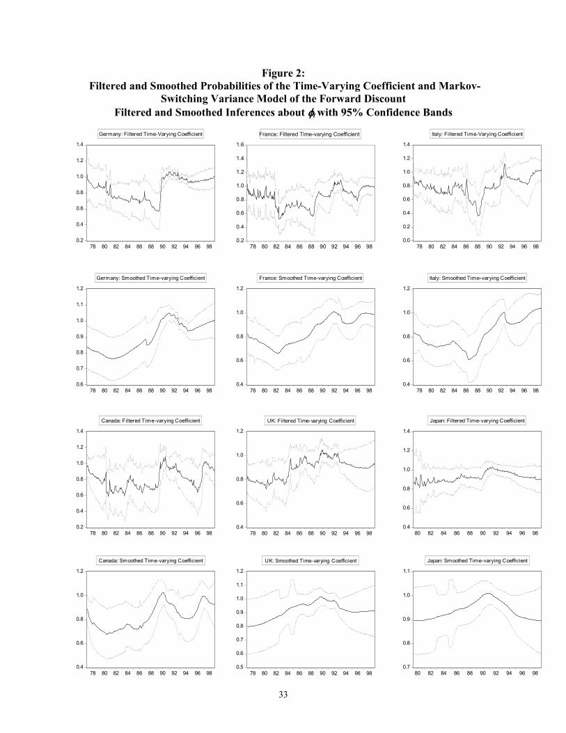
Figure 2 displays the results of the model applied to the six currencies. The

filtered inferences use information up to time t, and smoothed inferences use information 8 The complete details of the estimation technique can be found in Bai and Perron (1998) “Computation

13

from the entire sample, although all inferences are conditional on the hyper-parameters of

the model, which are estimated using the entire sample. With the exception of Japan, φt

exhibits substantial time variation. For the countries where time-variation is present, the

forward discount is not highly persistent throughout. Typically, the forward discount

starts out quite persistent at the beginning of the sample only to decline during the first

part of the 1980s, as low as 0.60 in the case of Germany for example. It becomes very

persistent again starting roughly at 1988. In all the cases considered, after that year φt

abruptly rises toward or even above unity and continues to exhibit unit-root-like behavior

until 1993. A possible interpretation for this behavior could be given along the lines of

Siklos and Granger (1996): There exist processes which are cointegrated most of the time

but not all the time. Perhaps forward and spot exchange rates fall into this category.

While this is an issue that deserves further investigation, we continue to assume

throughout the rest of the paper that spot and forward rates are and remain cointegrated

with a cointegrating vector of (1,-1)′.

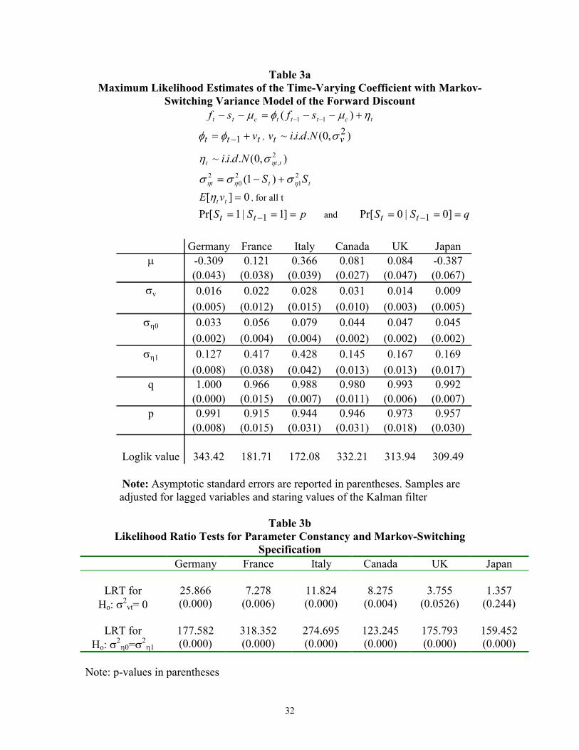
Table 3a reports the maximum likelihood estimates of the hyper-parameters.

Again, with the exception of Japan, the estimates of the variance for the time-varying

coefficient are all significant and of the same order of magnitude as the estimates of the

variance for the forward discount process in the low variance regime. The likelihood ratio

test statistics for the null hypothesis of no time variation are presented in table 3b. For

Germany, France, Italy, and Canada, the null hypothesis of parameter stability can be

rejected at the 1% level, while for the UK the same hypothesis can be rejected at the 5%

leve. However, parameter stability cannot be rejected in the case of Japan, even at the

10% level. Table 3b also presents likelihood ratio tests for the null hypothesis of constant

variance. It should be noted here that since the transition probabilities are not identified

under the null hypothesis, standard assumptions of asymptotic distribution theory do not

hold and the likelihood ratio test does not have a χ2 distribution. Hansen (1992) suggests

a computationally intensive method to determine the asymptotic distributions of the

relevant statistics. Instead, following Kim, Morley and Nelson (1999) we use a likelihood

ratio test using the critical values of Garcia (1995). Garcia derives asymptotic

distributions for a simple two-state Markov-switching model. The null hypothesis, and Analysis of Multiple Stuctural Change Models.”

14

2 20 ,0 ,1:H

η ησ σ= , is one of no Markov-switching. We compare these estimates to Garcia’s

most conservative critical values for a two-state Markov-switching mean and variance

model. He reports a critical value of 17.52 for a 1% significance level test. The

likelihood statistics for all the countries in our sample are much higher than this critical

value.

Figure 3 displays the filtered and smoothed probabilities of a low variance state.

The results are very similar across the different countries. It appears that the most volatile

state was the period during the latter part of the 1970s and the beginning of the 1980s.

Changes in monetary policy, abandonment of interest rates as an instrument and attention

to the monetary base, as well as the 1981-82 recession in the United States seem to be the

driving force. Other high volatility periods appear mostly as spikes during 1986, right

after the Plaza Accord Agreement, and again in September of 1992, when the ERM

collapsed. While we do not explicitly model possible volatility feedback effects to the

mean of the forward discount, figure 3 raises the possibility that the forward discount is

potentially subject to events that could lead to structural change.

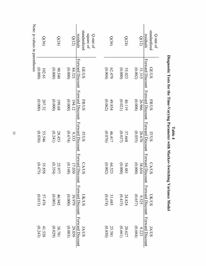
Table 4 presents some diagnostic tests for the model. We test for serial

correlation in both standardized forecast errors and the squares of the standardized

forecast errors. There is evidence of serial correlation for Germany and Canada for the

standardized forecast errors, as well as evidence of serial correlation for Germany, France

and less so UK in the square of the standardized forecast errors. This evidence suggests

that our two-state Markov-switching variance model has not captured completely the

heteroskedasticity pattern of the forward discount for these countries.9 However, the

time-varying parameter model seems to adequately capture the time series properties of

the forward discount process.

The estimates of the autoregressive coefficient provide evidence of parameter

instability, while the two distinct and persistent regimes of the variance suggest that

changes in policy could substantially affect the volatility of the forward discount. High

variance regimes are significant and are consistent with periods where policy changes are

9 We also tried a three-state Markov-switching variance specification for the countries in our sample. Although, the diagnostic tests where somewhat improved, the qualitative inferences regarding the autoregressive coefficient of the forward discount did not change. The results from the three-state specifications are available upon request.

15

in effect. The time-varying parameter model describes how the forward discount behavior

has changed over time. The next question that we are interested in addressing is why has

this behavior changed over the period of our sample. Eichenbaum and Evans (1995) show

that monetary shocks have a direct effect on the mean of the interest rate differential.

Thus in the next section we present such evidence using the Bai and Perron methodology

regarding partial multiple structural break models.

4.2 Partial Structural Break Model

Tables 5 and 6 present the results for the partial structural break models based on

(11). The determination of the existence of structural change and the selection of the

number of breaks depends on the values of various test statistics for structural change

when break dates are estimated and deserves some discussion. Let supFT(l) denote the F-

statistic for testing the null of no breaks (cj = c for all j) against the alternative of l breaks

(c1 ≠ c2 ≠ …≠ cl) where the break dates are selected according to (12). Define the double

maximum statistic )(supmaxmax 1 lFUD TLl≤≤= , where L is an upper bound on the

number of possible breaks. BP also consider a version of this statistic, denoted WDmax,

that applies weights to supFT(l) such that the marginal p-values are equal across values

of l. These statistics test the null hypothesis of no breaks against the alternative of an

unspecified number of breaks subject to a specified upper bound on the number of

breaks. Next, let supFT(l+1|l) denote the F-statistic for testing the null of l breaks against

the alternative of l+1 breaks. For this test the first l breaks are estimated and taken as

given. The statistic supFT(l+1|l) is then the maximum of the F-statistics for testing no

further structural change in the intercept against the alternative of one additional change

in the intercept when the break date is varied over all possible dates. All of these test

statistics have non-standard asymptotic distributions and BP provide the relevant critical

values.

BP (1998, 2000) suggest the following strategy for selecting the number of breaks

based on the above statistics. We first look at the UDmax or WDmax tests to see if at

least one break is present. If the null of no breaks is rejected, then the number of breaks

can be determined by looking at the sequential supFT(l+1|l) statistics. We select the

number of breaks for which the supFT(l+1|l) statistic is significant at least at the 5% level.

16

Table 5 presents the values of all the tests used to determine the number of breaks

for each country.10 In the case of Germany, the UDmax, and WDmax tests point to the

presence of multiple breaks. The supFT(l+1|l) tests suggests the use of a model with five

structural breaks since the supFT(5|4) test is significant at the 1% level. In the case of

France, the UDmax and WDmax tests reject the null hypothesis of no breaks versus the

alternative of an unknown number of breaks. The supFT(l+1|l) suggest that a model of

four breaks should be chosen over a model with three breaks. Notice that the supFT(2|1)

does not reject the null hypothesis of one break versus two. At the same time, the

supFT(l) does not reject the null of no breaks versus two but does reject the null when the

number of breaks is one, three, or four. Therefore, we estimate a model with four breaks

for France. For Japan neither the UDmax nor any of the WDmax tests point to a number

of breaks which is significantly different than zero. Hence, we do not estimate a model of

multiple structural breaks for Japan. Both the time-varying parameter model and the

stochastic break model single out Japan as the case where parameter instability, or

structural change is not statistically significant within our sample period.

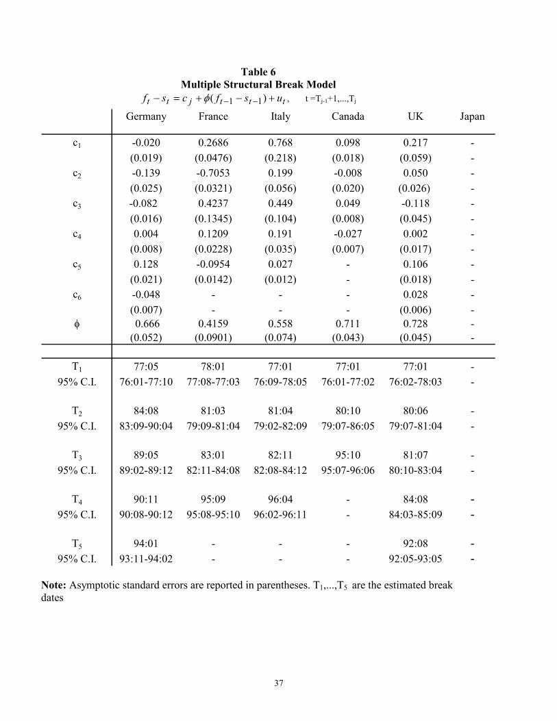
The results of the estimated break model (11) for the countries except Japan are

presented in table 6. Notice that all the point estimates of the φ coefficients across the

countries have dropped significantly compared to the estimates in table 2b, where we do

not account for structural breaks. For instance the autoregressive coefficient of the

forward discount was 0.939 for Germany and 0.907 for the UK when structural breaks

where not taken into account. The corresponding estimates are 0.666 and 0.728

respectively, when we allow for such breaks in the process.

In table 6 we also report the estimates of the break dates with their respective 95%

confidence intervals. Most of the break dates have been estimated quite accurately given

that the estimates of the confidence intervals span the period of about two years11. Also,

with the exception of the first and second break dates for Germany, the confidence

intervals do not overlap, suggesting that the number of breaks has also been estimated

accurately. Finally, most of the break dates estimated for each country are very similar to

the break dates for the rest of the countries, further attesting to the robustness of our 10 Critical values for these tests can be found in Bai and Perron (1998) 11 Because there is a lagged dependent variable in the break model (11), the adjustment after the break is gradual and depends on the value of the autoregressive coefficient.

17

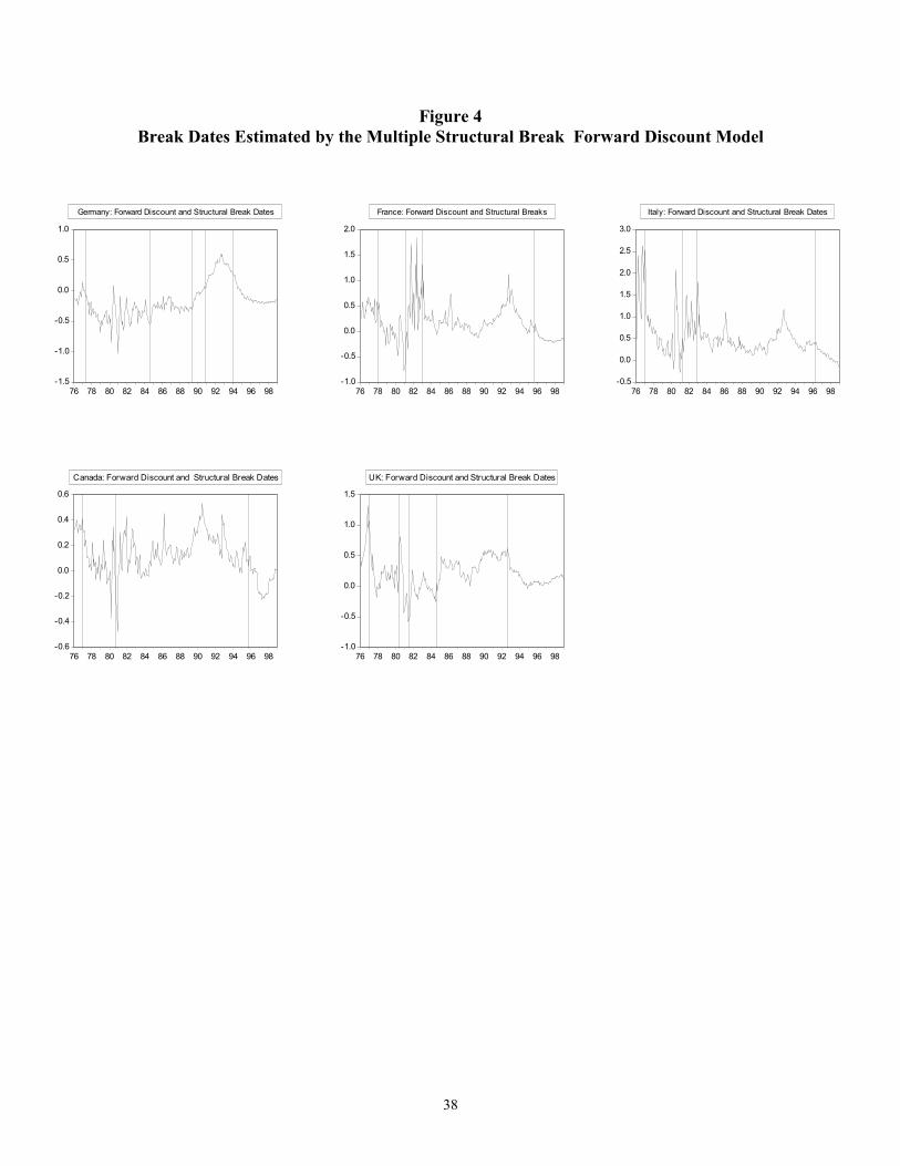
results. For all the countries, almost half of the breaks take place during the beginning of

the sample, coinciding with the first period of high volatility captured by the time-varying

coefficient model. This period is consistent with the change in the US central bank’s

policy objectives, as well as the subsequent recession of 1981-82. The break dates that

correspond to the US 1981-82 recession are identified for France, Italy, Canada, and the

UK as 1981:03, 1981:04, 1980:10, and 1981:07 respectively. Given our definition of the

exchange rate and covered interest parity, we can write:

UStttt iisf −=−

* (13)

where USti and *

ti represent the nominal interest rates in the US and the foreign country,

respectively. In all the cases, the implied unconditional means of the interest rate

differentials have changed significantly, for the duration of the regimes immediately

following the break dates.12

The final question we ask is the following: What are the implications of our

model, namely that the forward discount is not as persistent when structural breaks are

taken into account, for the forward discount puzzle? The estimate of β in equation (1) is

found consistently to be biased away from its theoretical value 1. Could our partial

structural change model explain some of this bias? In the next section we show using

Monte Carlo simulations that this is the case indeed. Although we impose FRUH, the

least squares point estimates of the coefficient turn out to be significantly biased

downward.

5. Monte-Carlo Simulations

In this section we use Monte Carlo simulations in order to assess the implications of

the presence of structural breaks in the forward discount process for FRUH. We estimate

the “differences regression” (1) and the AR(1) specification for the forward discount with

12 The estimates of the unconditional mean for France, Italy, Canada and the UK, before these breaks are –1.207, 0.450, -0.027, and –0.433 respectively. The means implied after the structural break date are 0.725, 1.015, 0.169, 0.007.

18

and without structural breaks in the mean of the forward discount. We report the

performance of the tests for whether β = 1 versus the alternatives of β ≠ 1 and β < 1 in

(1). We also report the performance of the unit root test for the autoregressive coefficient

of the forward discount. All experiments are based on 5000 replications.

5.1 Design of the Experiments

We employ an alternative yet equivalent representation of the cointegrating system

(9) as our data generating process. This representation is due to Phillips’ (1991) and is

called a triangular representation. For our purposes, the general form of the triangular

representation for yt is

,fttct usf ++= µ (12a) sttt uss +=

−1 (12b) where the vector of errors ut = (uft, ust)′ = (ft - st - µc, ∆st)′ has the VAR(1) representation

ut = Cut-1 + et where

,00

=

sC

β

φ

=

sss

sVσσ

σσ

η

ηηη

Equation (12a) models the structural co-integrating relationship and (12b) is a reduced

form relationship describing the stochastic trend in the spot rate. The VAR(1)

representation for ut implies

,1, ttfft uu ηφ +=

−

(12c) stftsst uu εβ +=

−1 (12d) Equation (12c) models the disequilibrium error (which equals the forward premium) as

an AR(1) process and (12d) allows the lagged error to affect the change in the spot rate.

Letting et = (ηt, εst)′. Note φ is the autoregressive coefficient of the forward discount and

β is the forward discount coefficient from equation (1). In our simulations we set βs = 1

so that UIP holds. In our monthly exchange rate data 0≈sησ . We calibrate forward and

19

spot exchange rates using the parameter estimates from the partial structural break model

of the forward discount reported in table 6. We also calibrate spot and forward rates

under the assumption of no break in the mean of the forward discount using the estimates

reported in table 2b. We estimate the differences regression (1), as well as the AR(1)

model of the forward discount using ordinary least squares. We also report the rejection

rates for testing that φ = 1 in the forward discount and βs = 1 in the differences regression.

Since φ = 1 is a unit root test its rejection rate really measures the power of the

augmented Dickey–Fuller test against the stationary alternative. Finally, in all the

experiments, we set the sample size, T = 250 to reflect the number of observations in our

actual data sample.

5.2 Monte Carlo Results

Tables 7 through 11 summarize the results of the Monte Carlo simulations for

each country. Notice that in the case of no structural breaks, both φ and βs are estimated

correctly. The adf test has very high power and the size of the t-test is a correct 5%. The

point estimates of βs range from 0.997 in the case of Italy, to 1.045 in the case of

Germany. The point estimates for φ are also extremely close to their true values.

When the data are generated under the assumption of structural breaks the results

of the Monte Carlo are quite different. Structural breaks, which are unaccounted for,

seem to produce two different yet interrelated results. First, the autoregressive coefficient

of the forward discount is estimated to be very high and the power of the adf test is

seriously reduced, with the exception of Italy and Canada. In both of these cases though,

the point estimates of φ are quite higher than their true values. For Germany, France and

the UK, the power of the adf test is 55.7%, 62.3%, and 25.2 % respectively.

Secondly, the point estimate of βs is seriously biased downward away from its

true value of 1. The point estimates range from 0.162 for Germany, which is the most

severe case of bias to 0.526 in the case of Canada. Moreover, the size of the t-test for the

null hypothesis of βs = 1 is distorted, forcing one to reject the null hypothesis more often

than she should. On average, at the 5% level, the two-sided t-test rejects the true null

hypothesis about 20% of the time, while the one-sided t-test’s rejection rate is even worse

at about 30%.

20

The results of the Monte Carlo simulations seem to justify our prior that the

forward premium is not as persistent as it appears to be. The presence of structural breaks

is responsible for generating I(1)-like behavior in its process, that contributes a

considerable degree of downward bias to the point estimate of β in equation (1). The

median estimate of β in our experiments is not negative, as usually is when actual

exchange rate data is estimated by least squares. Nevertheless, one would still mistakenly

reject the null hypothesis of forward rate unbiasdeness, if one did not account for the

presence of structural breaks in the forward discount.

6. Conclusion

We employ two different models of the forward discount under the prior that

structural breaks in its process could explain away the highly stylized fact of its high

persistence. The first model is a time varying parameter model with Markov-switching

variance that help us document the pattern of the persistence. We overwhemingly reject

the null hypothesis of no parameter instability for all G-7 countries with the exception of

Japan. The time varying parameter model is able to capture structural change that takes

place in a continuing fashion. The timing of the changes suggested the possibility of

structural breaks in the mean of the process. Thus, we proceed to use a stochastic partial

break model developed by Bai and Perron that explicitly allows for the incorporation and

estimation of structural breaks in the mean of a process. The stochastic break model can

be viewed as a plausible alternative to the fractionally integrated model of the forward

discount used by Baillie and Bollerslev (1998) and Maynard and Phillips (1998). We find

that breaks in the mean are present, and their timing coincides, at least for the case of the

1981-82 US recession with the types of monetary shocks reported by Eichenbaum and

Evans (1995). A contractionary shock to the US monetary policy increases the US

interest rates and, given our definition of the nominal exchange rate, also persistently

decreases the level of the forward discount which under covered interest parity is equal to

the interest rate differential of the two countries. Once these breaks are estimated, the

forward discount’s persistence is considerably lower than previously thought.

This finding has potentially important implications for what is known in the

International Finance literature as the “Forward Discount Anomaly.” In the absence of a

21

time-varying risk premium, we simulate spot and forward exchange rates under the

assumption of FRUH with and without incorporating breaks to the mean of the forward

discount. We find that when breaks are not accounted for, the least squares’ coefficient of

the forward discount in the “differences regression” is severely biased downward, away

from its theoretical value of 1. Furthermore, usual one- and two-sided t-tests suffer from

significant size distortion, forcing one to reject the null hypothesis of FRUH too often.

The forward discount puzzle is, to a considerable degree, a statistical artifact arising from

breaks in the mean of the forward discount. Since the median Monte Carlo estimates of

the forward discount coefficient in the “differences regression” are not negative, as is

usually reported when actual data is used, competing explanations of the bias may still be

valid and worth examining in light of our results. In particular, if a time-varying foreign

exchange rate risk premium does exist, what is its contribution to the bias, once structural

change has been accounted for? We hope to address this and related issues in the future.

22

APPENDIX A

Time-Varying Coefficient with Markov-Switching Variance Model13

Letting ]|Pr[ 1 iSjSp ttij ===−

with i=0,1 and j=0,1 , the Kalman filter for the

model described by equations (10) and (11) is given by:

i

ttji

tt 1|1),(

1| −−−

= ββ (A.1)

21|1

),(1| v

itt

jitt PP σ+=

−−−

(A.2)

tji

tttji

tt xy ),(1|

),(1| −−

−= βη (A.3)

2'),(1|

),(1| jt

jittt

jitt xPxf

εσ+=

−−

(A.4)

),(

1|),(

1|'),(

1|),(

1|),(

|

1 jitt

jittt

jitt

jitt

jitt fxP

−−−−

−

+= ηββ (A.5)

),(1|

),(1|

'),(1|

),(| )(

1 jittt

jittt

jitt

jitt PxfxPIP

−−−

−

−= (A.6)

where ]|[ 11| −−

Ψ≡ tttt E ββ , is the expectation of βt conditional on information up to time

t-1; Pt|t-1 is the variance of βt|t-1; ηt-1 is the forecast error and ft|t-1 is the variance of the

forecast error; yt ≡ ft - st, and xt ≡ ft-1 - st-1. Equations (A.1)-(A.4) are the prediction

equations of the Kalman Filter, while equations (A.5)-(A.6) are the updating equations.

We also need to use Hamilton’s (1989) filter which is given in the following three

steps:

Step 1: Given ]|Pr[ 11 −−

Ψ= tt iS , calculate

]|Pr[]|Pr[]|,Pr[ 11111 −−−=−−Ψ===Ψ== tttjtttt iSiSSiSjS (A.7)

where iSS tjt =−= 1|Pr[ ] is the transition probability

Step 2: Calculate the joint density of yt, St, St-1 and collapse across all possible states to

find the marginal density of yt:

13 This discussion follows Kim and Nelson (1999) “State-Space Models with Regime Switching”

23

]|,Pr[

),,|()|,,(

11

1111

−−

−−−−=

Ψ==

Ψ===Ψ=

ttt

ttttttjtt

iSjSiSjSyfiSSyf

(A.8)

Then the marginal density of yt is given by:

∑∑= =

−−=−=Ψ==Ψ

1

0

1

0111 )|,,()|(

j ittjtttt iSSyfyf

∑∑=

−−

=

−−Ψ==Ψ==

1

011

1

011 ]|,Pr[),,|(

jttt

itttt iSjSiSjSyf (A.9)

where =Ψ==−−

),,|( 11 tttt iSjSyf

),(1|

1),(1|

),(1|

21

),(1|

2 '21exp{||)2( ji

ttji

ttji

ttji

tt

T

ff−

−

−−

−

−

− ηηπ } (A.10)

Step 3: Update the joint probability of St and St-1 given yt and collapse across all possible

values of St-1:

)|(

)|,,(]|,Pr[

1

1111

−

−−

−−

Ψ

Ψ===Ψ==

tt

ttttttt yf

iSjSyfiSjS (A.11)

∑=

−Ψ===Ψ=

1

01 ]|,Pr[]|Pr[

ittttt iSjSjS (A.12)

Finally, as in Kim (1994) to complete the Kalman filter we collapse ),(|

jittβ and ),(

|ji

ttP

across all possible values for St-1:

]|Pr[

]|,Pr[1

0

),(|1

|tt

i

jittttt

jtt jS

iSjS

Ψ=

Ψ==

=

∑=

−β

β (A.13)

]|Pr[

}))((]{|,Pr[1

0

'),(||

),(||

),(|1

|tt

i

jitt

jtt

jitt

jtt

jittttt

jtt jS

PiSjSP

Ψ=

−−+Ψ==

=

∑=

−ββββ

(A.14)

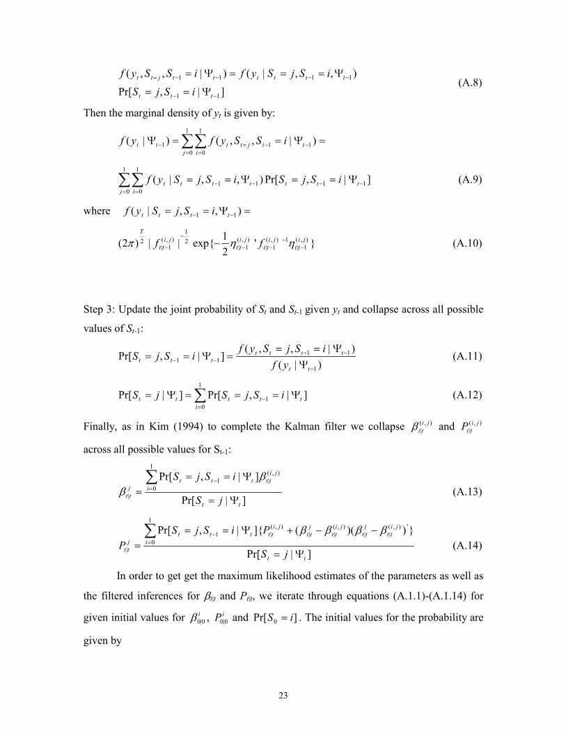
In order to get get the maximum likelihood estimates of the parameters as well as

the filtered inferences for βt|t and Pt|t, we iterate through equations (A.1.1)-(A.1.14) for

given initial values for i0|0β , iP 0|0 and ]Pr[ 0 iS = . The initial values for the probability are

given by

24

qp

pS−−

−

==

21]0Pr[ 0 and

pqqS−−

−

==

21]1Pr[ 0 (A.15)

Since βt| has no unconditional expectation under the random walk specification, we have

no choice but to make an arbitrary guess as to its initial value and then assign a very large

variance to our guess, i.e., 00|0 =iβ and ∞≈

iP 0|0 . We then use the first τ observations to

determine iττ

β | and iPττ | and use these values as the initial values for the maximum

likelihood estimation.

The filtered inferences about βt and the confidence bands based on Pt|t are given

by:

∑=

Ψ==

1

0|| ]|Pr[

j

jtttttt jS ββ (A.16)

}))(({]|Pr[ '|||||

1

0|

jtt

jtt

jtttt

jtt

jtttt PjSP ββββ −−+Ψ==∑

=

(A.17)

The parameters of the model can be estimated by:

∑+=

−Ψ=

T

tttyfl

11 )|(ln)(max

τθ

θ (A.18)

Using Kim’s (1994) smoothing algorithm, we can also obtain the smoothed

probability ]|0Pr[ TtS Ψ= . This is accomplished by iterating backward through the

following equations (conditional on St = j and St+1 = l, where j = 0,1 and l = 0,1):

]|Pr[

]|Pr[]|Pr[]|Pr[]|,Pr[

1

11

11

Tt

ttttTt

Ttt

lSjSlSjSlS

jSlS

Ψ=

==Ψ=Ψ=

=Ψ==

+

++

++

(A.19)

]|,Pr[]|Pr[1

0111 ∑

=

+++Ψ===Ψ=

lTttTt jSlSjS (A.20)

Finally, we can obtain smoothed inferences about βt conditional up to Information

T, using the smoothed probabilities given by equations (A.19)-(A.20), and iterating

backward the following two equations:

)( ),(|1|1

),(|1||

),(|

1 ljTt

lTt

ljtt

jtt

jtt

ljTt PP

+++−+=

−

ββββ (A.21)

)')()((11 ),(

|1|),(

|1|1),(

|1||),(

|

−−

++++−+=

ljtt

jtt

ljtt

lTt

ljtt

jtt

jtt

ljTt PPPPPPPP (A.22)

25

References

Bai, Jushan (1997b): “Estimating multiple breaks one at a time,” Econometric theory, 13, 315-352.

Bai, Jushan and Pierre Perron (1998): “Estimating and testing linear models with multiple

structural changes,” Econometrica, 66, 47-78. ____ (2000): “Computation and analysis of multiple structural change models,” working

paper, Department of Economics, Boston College. Baillie, Richard T. and Tim Bollerslev (1994): “The long memory of the forward

premium,” Journal of International Money and Finance, 11, 208-219. Baillie, Richard T. and Tim Bollerslev (2000): “The forward premium anomaly is not as

bad as you think Journal of International Money and Finance. Bilson, John F.0. (1981): “The ‘speculative efficiency’ hypothesis,” Journal of Business,

54, 435-51. Campbell, John Y. and Pierre Perron (1991): “Pitfalls and opportunities: What

macroeconomists should know about unit roots and cointegration,” NBER Macroeconomics Annual. MIT Press, Cambridge, MA.

Choi, K., and Zivot, E. (2001). “Long memory and structural breaks in the forward

discount,” manuscript in preparation, Department of Economics, University of Washington.

Christiano, Lawrence J., Martin Eichenbaum and Charles L. Evans (): “Monetary policy

shocks: What have we learned and to what end?” NBER, working paper 6400. Clarida, Richard and Mark Gertler (1997): “How the Bundesbank conducts Monetary

policy,” in Reducing inflation: motivation and strategy, University of Chicago Press, Chicago.

Crowder, William J. (1994): “Foreign exchange market efficiency and common

stochastic trends,” Journal of International Money and Finance, 13, 551-564. Cushman, David O. and Tao Zha (1997): “Identifying monetary policy in a small open

economy under flexible exchange rates,” Journal of Monetary Economics, 39, 4. Diebold, Francis X. and Atsushi Inoue (1999): “Long memory and structural change,”

working paper, University of Pennsylvania.

26

Dominguez, Kathryn M. (1998): “Central bank intervention and exchange rate volatility,” Journal of International Money and Finance, 17, 161-190.

Eichenbaum Martin, and Charles L. Evans (1995): “Some empirical evidence on the

effects of shocks to monetary policy on exchange rates,” The Quarterly Journal of Economics, Vo. 110, 4, 1975-1010.

Engel, Charles (1996): “The forward discount anomaly and the risk premium: A survey

of recent evidence,” Journal of Empirical Finance, 3, 123-192. Engle, R.F and M. Watson (1987): Kalman filter: applications to forecasting and rational

expectation models, Advances in Econometrics, Fifth World Congress, Vol.1,245-281.

Evans, Martin D.D. and Karen Lewis (1995): “Do long-term swings in the dollar affect

estimates of the risk premia?” Review of Financial Studies, Vol. 8, No. 3, 709-742. Fama, Eugene (1984a): “Forward and spot exchange rates,” Journal of Monetary

Economics, 14, 319-338. Froot, Kenneth A. (1990): “Short rates and expected asset returns,” working paper no.

3247, National Bureau of Economic Research, Cambridge, MA. Froot, Kenneth A. and Jeffrey A. Frankel (1989): “Forward discount bias: is it an

exchange risk premium?” Quarterly Journal of Economics, 104, 139-61. Froot, Kenneth A. and Richard H. Thaler (1990): “Anomalies: Foreign exchange,” The

Journal of Economic Perspectives, Vol. 4, 3, 179-192. Garbade, K. (1977): Two methods for examining the stability of regression coefficients,

Journal of the American Statistical Association, 72, 54-63. Garcia, Rene (1995): “Asymptotic null distribution of the likelihood ratio test in Markov

switching models”, manuscript, University of Montreal. Garcia, Rene and Pierre Perron (1996): “An analysis of the real interest rate under regime

shifts,” Review of Economics and Statistics, 78, 111-125. Godbout, Marie-Josee and Simon van Norden (1996): “Unit root tests and excess

returns,” working paper 96-10, Bank of Canada. Granger, Clive W.J. (1999): “Aspects of research strategies for time series analysis,”

presentation to the conference on New Developments in Time Series Economics, New Haven, October 99.

27

Hai, Weike, Nelson Mark and Yangru Wu (1997): “Understanding spot and forward exchange rate regressions,” Journal of Apllied Econometrics, Vol. 12, No. 6, 715-734.

Hamilton, James (1993): Time Series Analysis, Princeton University Press, Princeton, NJ. Hansen, Bruce E. (1992): “The likelihood ratio test under nonstandard conditions: testing

the Markov switching model of GNP,” Journal of Applied Econometrics, 64, 307-333.

Horvath, Michael T.K and Mark W. Watson (1995): “Testing for cointegration when

some of the cointegrating vectors are prespecified,” Econometric Theory, 11, 984-1015.

Kim, Chang-Jin and Charles R. Nelson (1999): State-space models with regime

switching, classical and Gibbs-sampling approaches with applications, MIT Press, Cambridge, Massachusetts.

Kim, Chang-Jin, James C. Morley, and Charles R. Nelson (1999): “Do changesin the

market risk premiumexplain the empirical evidence of mean reversion in stock prices?” working paper, Department of Economics, University of Washington, Seattle, WA.

Kim, Souyong and Nouriel Roubini (1995): “Liquidity and exchange rates, a structural

VAR approach,” manuscript, New York University. Lewis, Karen K. (1989): “Changing beliefs and systematic rational forecast errors with

evidence from foreign exchange,” The American Economic Review,Vol. 79, 4, 621-636.

____ (1995): Puzzles in international financial markets, Handbook of International

Economics Volume 3, Elsevier Science B.V., Amsterdam, Netherlands Mark, Nelson C. and Yangru Wu (1998): “Rethinking deviations from uncovered interest

parity: The role of covariance risk and noise,” The Economic Journal, 108, 1686-1706.

Marston, Richard C. (1995): International financial integration: A study of interest

differentials between the major industrial countries, Cambridge University Press, New York, New York.

Maynard Alex and Peter C.B. Phillips (1998): “Rethinking an old empirical puzzle:

Econometric evidence on the forward discount anomaly,'” working paper, Yale University.

28

Perron, Pierre (1989): “The great crash, the oil price shock and the unit root hypothesis,” Econometrica, 57, 1361-1401.

Phillips, Peter C.B. (1991):Optimal inference in cointegrated systems,” Econometrica,

60, 119-143. Sargan, J.D. (1964): “Wages and prices in the United Kingdom: a study in econometric

methodology,” in P.E Hart, G. Mills and J.K. Whitaker (eds.), Econometric Analysis for National Economic Planning, London: Butterworths, 25-54.

Siklos, Pierre L. and Clive W. Granger (1996): “Temporary cointegration with an

application to interest rate parity,” UCSD Discussion Paper No 96-11. Wang, Jiahui and Eric Zivot (2000): “A Bayesian time series model of multiple

structural changes in level, trend and variance,” Journal of Business and Economic Statistics.

Zivot, Eric (1999): “Cointegration and Forward and Spot Exchange Ratesforthcoming in

the Journal of International Money and Finance.

29

Figure 1 Monthly Forward Discount

Source: Datastream

-1.0

-0.5

0.0

0.5

1.0

1.5

76 78 80 82 84 86 88 90 92 94 96 98

UK/US Forward Discount

-1.5

-1.0

-0.5

0.0

0.5

1.0

76 78 80 82 84 86 88 90 92 94 96 98

GE/US Forward Discount

-1.0

-0.5

0.0

0.5

1.0

1.5

2.0

76 78 80 82 84 86 88 90 92 94 96 98

FRA/US Forward Discount

-0.5

0.0

0.5

1.0

1.5

2.0

2.5

3.0

76 78 80 82 84 86 88 90 92 94 96 98

ITA/US Forward Discount

-0.6

-0.4

-0.2

0.0

0.2

0.4

0.6

76 78 80 82 84 86 88 90 92 94 96 98

CA/US Forward Discount

-1.2

-0.8

-0.4

0.0

0.4

76 78 80 82 84 86 88 90 92 94 96 98

JA/US Forward Discount

30

T

able 1a: Summ

ary Statistics For Exchange R

ate Data

Table 1b: Sum

mary Statistics For Exchange R

ate Data

Note: ρ

1 denotes the first order autocorrelation coefficient.

Germ

an Mark

French FrancItalian Lira

∆s

t+1

∆f

t+1

ft -s

t∆

st+

1∆

ft+

1f

t -st

∆s

t+1

∆f

t+1

ft -s

t

mean

-0.164-0.157

-0.1630.080

0.0800.176

0.3190.277

0.500

sd3.325

3.3260.279

3.2353.197

0.3313.241

3.1760.432

ρ1-0.012

-0.0150.939

-0.011-0.003

0.6960.075

0.0750.791

Correla

1.0000.999

-0.0571.000

0.9960.036

1.0000.996

0.07tion

1.000-0.062

1.0000.005

1.0000.042

Matrix

1.0001.000

1.000

Canadian D

ollarBritish Pound

Japanese Yen∆

st+

1∆

ft+

1f

t -st

∆s

t+1

∆f

t+1

ft -s

t∆

st+

1∆

ft+

1f

t -st

mean

0.1490.155

0.1130.070

0.0710.215

-0.360-0.237

-0.296

sd1.379

1.3870.162

3.2893.295

0.263.670

3.7650.259

ρ1-0.088

-0.0920.839

0.0840.086

0.907-0.001

-0.0040.928

Correla

1.0000.997

-0.1541.000

0.999-0.124

1.0000.999

-0.184tion

1.000-0.171

1.000-0.131

1.000-0.189

Matrix

1.0001.000

1.000

31

Table 2a: Estimates of the Differences Regression

OLS: tttt sfs εβα +−+=∆+

)(1

German French Italian Canadian British Japanese Mark Franc Lira Dollar Pound Yen

α -0.269 0.0191 0.019 0.305 0.411 -1.031(0.240) (0.239) (0.293) (0.099) (0.239) (0.316)

t α=0 -1.12083 0.0795 0.06485 3.08081 1.71967 -3.26266(0.868) (0.468) (0.474) (0.001) (0.043) (0.000)

β -0.686 0.352 0.518 -1.304 -1.568 -2.680(0.909) (0.873) (0.484) (0.506) (0.856) (0.090)

t β=1 -1.85 -0.74 -1.00 -4.55 -3.00 -40.89(0.032) (0.229) (0.159) (0.000) (0.001) (0.000)

σ1/2

ss 3.33 3.241 3.182 1.377 3.295 3.768

R 2 0.003 0.001 0.004 0.023 0.015 0.034 Note: White heteroskedasticity-consistent standard errors in parentheses. tβ=1 denotes the two-tail t-statistic for H0: 1=β . p-values are in bold parentheses. Table 2b: Estimates of the AR(1) specification of the Forward Discount

OLS: tvtstfctstf +

−−

−+=− )11(φ

Note: White heteroskedasticity-consistent standard errors in parentheses

German French Italian Canadian British Japanese Mark Franc Lira Dollar Pound Yen

c -0.009 0.052 0.099 0.0169 0.018 -0.020(0.005) (0.016) (0.026) (0.009) (0.010) (0.008)

φ 0.939 0.698 0.797 0.840 0.907 0.928(0.028) (0.108) (0.062) (0.053) (0.038) (0.031)

σ1/2

v 0.279 0.331 0.433 0.162 0.260 0.259

R 2 0.882 0.486 0.630 0.710 0.824 0.864

32

Table 3a Maximum Likelihood Estimates of the Time-Varying Coefficient with Markov-

Switching Variance Model of the Forward Discount tctttctt sfsf ηµφµ +−−=−−

−−

)( 11

ttt v+=−1φφ , ),0(...~ 2

vt Ndiiv σ

0][ =tt vE η , for all t

pSS tt ===−

]1|1Pr[ 1 and qSS tt ===−

]0|0Pr[ 1

Note: Asymptotic standard errors are reported in parentheses. Samples are adjusted for lagged variables and staring values of the Kalman filter

Table 3b

Likelihood Ratio Tests for Parameter Constancy and Markov-Switching Specification

Germany France Italy Canada UK Japan

LRT for Ho: σ2

vt= 0 25.866 (0.000)

7.278 (0.006)

11.824 (0.000)

8.275 (0.004)

3.755 (0.0526)

1.357 (0.244)

LRT for

Ho: σ2η0=σ2

η1 177.582 (0.000)

318.352 (0.000)

274.695 (0.000)

123.245 (0.000)

175.793 (0.000)

159.452 (0.000)

Note: p-values in parentheses

ttt SS 21

20

2 )1(ηηη

σσσ +−=

),0(...~ 2,ttt Ndii

ηση

Germany France Italy Canada UK Japanµ -0.309 0.121 0.366 0.081 0.084 -0.387

(0.043) (0.038) (0.039) (0.027) (0.047) (0.067)σv 0.016 0.022 0.028 0.031 0.014 0.009

(0.005) (0.012) (0.015) (0.010) (0.003) (0.005)ση0 0.033 0.056 0.079 0.044 0.047 0.045

(0.002) (0.004) (0.004) (0.002) (0.002) (0.002)ση1 0.127 0.417 0.428 0.145 0.167 0.169

(0.008) (0.038) (0.042) (0.013) (0.013) (0.017)q 1.000 0.966 0.988 0.980 0.993 0.992

(0.000) (0.015) (0.007) (0.011) (0.006) (0.007)p 0.991 0.915 0.944 0.946 0.973 0.957

(0.008) (0.015) (0.031) (0.031) (0.018) (0.030)

Loglik value 343.42 181.71 172.08 332.21 313.94 309.49

33

Figure 2: Filtered and Smoothed Probabilities of the Time-Varying Coefficient and Markov-

Switching Variance Model of the Forward Discount Filtered and Smoothed Inferences about φφφφt with 95% Confidence Bands

0.2

0.4

0.6

0.8

1.0

1.2

1.4

78 80 82 84 86 88 90 92 94 96 98

Germany: Filtered Time-Varying Coefficient

0.0

0.2

0.4

0.6

0.8

1.0

1.2

1.4

78 80 82 84 86 88 90 92 94 96 98

Italy: Filtered Time-Varying Coefficient

0.4

0.6

0.8

1.0

1.2

78 80 82 84 86 88 90 92 94 96 98

Italy: Smoothed Time-varying Coefficient

0.4

0.6

0.8

1.0

1.2

78 80 82 84 86 88 90 92 94 96 98

France: Smoothed Time-varying Coefficient

0.6

0.7

0.8

0.9

1.0

1.1

1.2

78 80 82 84 86 88 90 92 94 96 98

Germany: Smoothed Time-varying Coefficient

0.2

0.4

0.6

0.8

1.0

1.2

1.4

78 80 82 84 86 88 90 92 94 96 98

Canada: Filtered Time-varying Coefficient

0.4

0.6

0.8

1.0

1.2

78 80 82 84 86 88 90 92 94 96 98

Canada: Smoothed Time-varying Coefficient

0.4

0.6

0.8

1.0

1.2

1.4

80 82 84 86 88 90 92 94 96 98

Japan: Filtered Time-varying Coefficient

0.7

0.8

0.9

1.0

1.1

80 82 84 86 88 90 92 94 96 98

Japan: Smoothed Time-varying Coefficient

0.4

0.6

0.8

1.0

1.2

78 80 82 84 86 88 90 92 94 96 98

UK: Filtered Time-varying Coefficient

0.5

0.6

0.7

0.8

0.9

1.0

1.1

1.2

78 80 82 84 86 88 90 92 94 96 98

UK: Smoothed Time-varying Coefficient

0.2

0.4

0.6

0.8

1.0

1.2

1.4

1.6

78 80 82 84 86 88 90 92 94 96 98

France: Filtered Time-varying Coefficient

34

Figure 3 Time-Varying Coefficient and Markov-Switching Variance Model

Filtered and Smoothed Probabilities of the Low Variance State

0.0

0.2

0.4

0.6

0.8

1.0

78 80 82 84 86 88 90 92 94 96 98

Germany: Filtered Probability of Low Variance Regime

0.0

0.2

0.4

0.6

0.8

1.0

78 80 82 84 86 88 90 92 94 96 98

France: Filtered Probability of Low Variance Regime

0.0

0.2

0.4

0.6

0.8

1.0

78 80 82 84 86 88 90 92 94 96 98

Italy: Filtered Probability of Low Variance Regime

0.0

0.2

0.4

0.6

0.8

1.0

78 80 82 84 86 88 90 92 94 96 98

Germany: Smoothed Probability of Low Variance Regime

0.0

0.2

0.4

0.6

0.8

1.0

78 80 82 84 86 88 90 92 94 96 98

France: Smoothed Probability of Low Variance Regime

0.0

0.2

0.4

0.6

0.8

1.0

78 80 82 84 86 88 90 92 94 96 98

Italy: Smoothed Probability of Low Variance Regime

0.0

0.2

0.4

0.6

0.8

1.0

78 80 82 84 86 88 90 92 94 96 98

Canada: Filtered Probability of Low Variance Regime

0.0

0.2

0.4

0.6

0.8

1.0

78 80 82 84 86 88 90 92 94 96 98

Canada: Smoothed Probability of Low Variance Regime

0.0

0.2

0.4

0.6

0.8

1.0

80 82 84 86 88 90 92 94 96 98

Japan: Filtered Probability of Low Variance Regime

0.0

0.2

0.4

0.6

0.8

1.0

78 80 82 84 86 88 90 92 94 96 98

UK: Filtered Probability of Low Variance Regime

0.0

0.2

0.4

0.6

0.8

1.0

78 80 82 84 86 88 90 92 94 96 98

UK: Smoothed Probability of Low Variance Regime

0.0

0.2

0.4

0.6

0.8

1.0

80 82 84 86 88 90 92 94 96 98

Japan: Smoothed Probabili ty of Low Variance Regime

35

Table 4

Diagnostic T

ests for the Tim

e-Varying Param

eter with M

arkov-Switching V

ariance Model

Q-stat of

standardized G

E/US

FR/U

SIT/U

SC

A/U

SU

K/U

SJA

/US

residualsForw

ard Discount

Forward D

iscountForw

ard Discount

Forward D

iscountForw

ard Discount

Forward D

iscountQ

(12)31.315

26.96620.670

38.6549.525

9.223(0.002)

(0.008)(0.055)

(0.000)(0.657)

(0.684)

Q(24)

55.02340.119

37.66854.481

24.82420.627

(0.000)(0.021)

(0.037)(0.000)

(0.415)(0.661)

Q(36)

62.47049.854

46.41764.523

31.68525.581

(0.004)(0.062)

(0.076)(0.002)

(0.674)(0.850)

Q-stat of

square ofstandardized

GE/U

S FR

/US

IT/US

CA

/US

UK

/US

JA/U

Sresiduals

Forward D

iscountForw

ard Discount

Forward D

iscountForw

ard Discount

Forward D

iscountForw

ard Discount

Q(12)

84.321194.12

9.33317.030

39.97929.859

(0.000)(0.000)

(0.674)(0.148)

(0.000)(0.003)

Q(24)

90.540199.68

28.45325.977

46.94538.781

(0.000)(0.000)

(0.241)(0.354)

(0.003)(0.029)

Q(36)

102.61207.32

53.54635.858

57.47641.520

(0.000)(0.000)

(0.030)(0.475)

(0.013)(0.243)

Note: p-values in parentheses

36

Table 5 Structural Break Tests for the Multiple Structural Break Forward Discount Model

Note: a, b, c denote 1%, 5%, and 10% levels of significance respectively

Wdmax(1%) 20.510a 32.930a 17.752a 7.934a 14.446 9.017

SupFT(2|1) 31.183a 8.579 27.040a 10.486c 5.204 13.005b

SupFT(3|2) 10.550c 38.887a 7.69 19.932a 9.22 13.005b

SupFT(4|3) 12.807c 18.462a 30.293a 10.486 14.550b 13.005b

SupFT(5|4) 29.109a 6.461 7.69 8.128 14.550b 11.691c

Decision: numberof breaks 5 4 4 3 5 0

37

Table 6 Multiple Structural Break Model

tttjtt usfcsf +−+=−−−

)( 11φ , t =Tj-1+1,...,Tj

Germany France Italy Canada UK Japan

c1 -0.020 0.2686 0.768 0.098 0.217 -(0.019) (0.0476) (0.218) (0.018) (0.059) -

c2 -0.139 -0.7053 0.199 -0.008 0.050 -(0.025) (0.0321) (0.056) (0.020) (0.026) -

c3 -0.082 0.4237 0.449 0.049 -0.118 -(0.016) (0.1345) (0.104) (0.008) (0.045) -

c4 0.004 0.1209 0.191 -0.027 0.002 -(0.008) (0.0228) (0.035) (0.007) (0.017) -

c5 0.128 -0.0954 0.027 - 0.106 -(0.021) (0.0142) (0.012) - (0.018) -

c6 -0.048 - - - 0.028 -(0.007) - - - (0.006) -

φ 0.666 0.4159 0.558 0.711 0.728 -(0.052) (0.0901) (0.074) (0.043) (0.045) -

T1 77:05 78:01 77:01 77:01 77:01 -95% C.I. 76:01-77:10 77:08-77:03 76:09-78:05 76:01-77:02 76:02-78:03 -

T2 84:08 81:03 81:04 80:10 80:06 -95% C.I. 83:09-90:04 79:09-81:04 79:02-82:09 79:07-86:05 79:07-81:04 -

T3 89:05 83:01 82:11 95:10 81:07 -95% C.I. 89:02-89:12 82:11-84:08 82:08-84:12 95:07-96:06 80:10-83:04 -

T4 90:11 95:09 96:04 - 84:08 -95% C.I. 90:08-90:12 95:08-95:10 96:02-96:11 - 84:03-85:09 -

T5 94:01 - - - 92:08 -95% C.I. 93:11-94:02 - - - 92:05-93:05 -

Note: Asymptotic standard errors are reported in parentheses. T1,...,T5 are the estimated break dates

38

Figure 4 Break Dates Estimated by the Multiple Structural Break Forward Discount Model

-1.5

-1.0

-0.5

0.0

0.5

1.0

76 78 80 82 84 86 88 90 92 94 96 98

Germany: Forward Discount and Structural Break Dates

-1.0

-0.5

0.0

0.5

1.0

1.5

2.0

76 78 80 82 84 86 88 90 92 94 96 98

France: Forward Discount and Structural Breaks

-0.5

0.0

0.5

1.0

1.5

2.0

2.5

3.0

76 78 80 82 84 86 88 90 92 94 96 98

Italy: Forward Discount and Structural Break Dates

-0.6

-0.4

-0.2

0.0

0.2

0.4

0.6

76 78 80 82 84 86 88 90 92 94 96 98

Canada: Forward Discount and Structural Break Dates

-1.0

-0.5

0.0

0.5

1.0

1.5

76 78 80 82 84 86 88 90 92 94 96 98

UK: Forward Discount and Structural Break Dates

39

Table 7 Monte Carlo Estimates of the Forward Discount and “Differences” Regressions

Germany

tftftfttct uuusf ηφµ +=++=−1,

stftststtt uuuss εβ +=+=−− 11 ,

=

2

2

325.300088.0

,00

iidNst

t

ε

η

Estimated regression: ft-st = c + φ(ft-1-st-1) + et

T = 250 Structural Breaks No Structural

Breaks c φ ADF c φ ADF

β=1 0.003 0.919 -2.92 -0.009 0.655 -6.251

φ =0.666 (0.557)b (0.995)b

Estimated regression: ∆st+1 = α + β(ft-st) + vt+1


Breaks

β=1 α β tβ=1 α β tβ=1 φ =0.666 -0.012 0.162 -1.198 0.027 1.045 -0.003

(0.217)a (0.055)a

(0.323)b (0.050)b

Note: φ

µ−

=

1c

c is the unconditional mean of the forward discount. When we estimate the

model with no structural breaks c = -0.009, the estimate from table 2b. When we estimate the model with structural breaks then c is set to the estimates given in table 6. We report the median estimates of the parameters based on 5,000 simulations. The values in parentheses indicate the empirical rejection frequency of nominal 5% two-sided testsa and one-sided testsb.

40

Table 8 Monte Carlo Estimates of the Forward Discount and “Differences” Regressions

France

tftftfttct uuusf ηφµ +=++=−1,

stftststtt uuuss εβ +=+=−− 11 ,

=

2

2

235.300214.0

,00

iidNst

t

ε

η




β=1 0.004 0.874 -2.991 0.052 0.409 -8.048

φ =0.415 (0.623)b (0.998)b



Breaks

β=1 α β tβ=1 α β tβ=1 φ =0.415 -0.005 0.143 -2.545 -0.091 1.004 -0.032

(0.719)a (0.050)a

(0.811)b (0.052)b

Note: φ

µ−

=

1c


model with no structural breaks c = 0.052, the estimate from table 2b. When we estimate the model with structural breaks then c is set to the estimates given in table 6. We report the median estimates of the parameters based on 5,000 simulations. The values in parentheses indicate the empirical rejection frequency of nominal 5% two-sided testsa and one-sided testsb.

41

Table 9

Monte Carlo Estimates of the Forward Discount and “Differences” Regressions Italy

tftftfttct uuusf ηφµ +=++=

−1, stftststtt uuuss εβ +=+=

−− 11 ,

=

2

2

241.300242.0

,00

iidNst

t

ε

η




β=1 0.144 0.728 -4.191 0.101 0.547 -7.068

φ =0.558 (0.983)b (0.999)b



Breaks

β=1 α β tβ=1 α β tβ=1 φ =0.558 -0.248 0.472 -1.087 -0.219 0.997 -0.033

(0.196)a (0.053)a

(0.288)b (0.052)b

Note: φ

µ−

=

1c



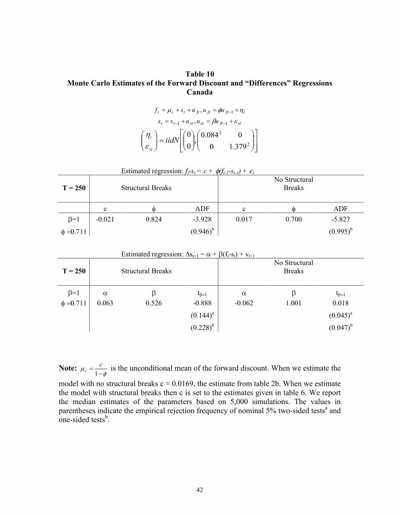
42

Table 10

Monte Carlo Estimates of the Forward Discount and “Differences” Regressions Canada



−− 11 ,

=

2

2

379.100084.0

,00

iidNst

t

ε

η




β=1 -0.021 0.824 -3.928 0.017 0.700 -5.827

φ =0.711 (0.946)b (0.995)b



Breaks

β=1 α β tβ=1 α β tβ=1 φ =0.711 0.063 0.526 -0.888 -0.062 1.001 0.018

(0.144)a (0.045)a

(0.228)b (0.047)b

Note: φ

µ−

=

1c



43

Table 11

Monte Carlo Estimates of the Forward Discount and Differences Regressions UK



−− 11 ,

=

2

2

289.300100.0

,00

iidNst

t

ε

η




β=1 0.017 0.897 -2.471 0.0187 0.717 -5.636

φ =0.728 (0.252)b (0.996)b



Breaks

β=1 α β tβ=1 α β tβ=1 φ =0.728 -0.031 0.214 -1.157 -0.064 1.019 -0.015

(0.212)a (0.048)a

(0.307)b (0.046)b

Note: φ

µ−

=

1c



Documents

Time-Variation and Structural Change in the Forward