Time-Varying Arrival Rates of Informed and …pages.stern.nyu.edu › ~rengle › EngleEasleyOharaWu.pdfJournal of Financial Econometrics, 2008, 171–207 Time-Varying Arrival Rates

Journal of Financial Econometrics, 2008, 171–207

Time-Varying Arrival Rates of Informedand Uninformed TradesDavid Easley

Cornell University

Robert F. Engle

New York University

Maureen O’Hara

Cornell University

Liuren Wu

Baruch College, CUNY

abstract

We propose a dynamic econometric microstructure model of trading, and weinvestigate how the dynamics of trades and trade composition interact withthe evolution of market liquidity, market depth, and order flow. We estimatea bivariate generalized autoregressive intensity process for the arrival rates ofinformed and uninformed trades for 16 actively traded stocks over 15 yearsof transaction data. Our results show that both informed and uninformedtrades are highly persistent, but that the uninformed arrival forecasts respondnegatively to past forecasts of the informed intensity. Our estimation generatesdaily conditional arrival rates of informed and uninformed trades, which weuse to construct forecasts of the probability of information-based trade (PIN).These forecasts are used in turn to forecast market liquidity as measured bybid-ask spreads and the price impact of orders. We observe that PINs varyacross assets and over time, and most importantly that they are correlatedacross assets. Our analysis shows that one principal component explainsmuch of the daily variation in PINs and that this systemic liquidity factor may be

We thank Mark Ready, Schmuel Baruch, and seminar participants at New York University and the 2002AFA meetings for helpful comments. Address correspondence to Robert F. Engle, Stern School of Busi-ness, New York University, 44 West 4th Street, Suite 9-62, NY 10012-1126, or e-mail: [email protected].

doi: 10.1093/jjfinec/nbn003Advance Access publication February 26, 2008C© The Author 2008. Published by Oxford University Press. All rights reserved. The online version of thisarticle has been published under an open access model. Users are entitled to use, reproduce, disseminate,or display the open access version of this article for non-commercial purposes provided that: the originalauthorship is properly and fully attributed; the Journal and Oxford University Press are attributed as theoriginal place of publication with the correct citation details given; if an article is subsequently reproducedor disseminated not in its entirety but only in part or as a derivative work this must be clearly indicated. Forcommercial re-use, please contact [email protected]

172 Journal of Financial Econometrics

important for asset pricing. We also find that PINs tend to rise before earningsannouncement days and decline afterwards. ( JEL: C51, C53, G10, G12, G14)

keywords: Arrival rates, informed trades, uninformed trades, autoregres-sive process, market depth, liquidity

A fundamental insight of the microstructure literature is that order flow is informa-tive regarding subsequent price movements. This informational role arises becauseorders arrive from both informed and uninformed traders, and market observerscan infer new information regarding the value of the asset from the compositionand existence of trades. Thus, market parameters such as volume, volatility, mar-ket depth, and liquidity are all linked in the sense that each is influenced by theunderlying order arrival processes. In this paper, we propose a dynamic econo-metric microstructure model of trading, and we investigate how the dynamicsof trades and trade composition interact with the evolution of market liquidity,market depth, and order flows.

There are many reasons why understanding market liquidity and depth areimportant. From a practical perspective, the cost of trading in a security is inex-tricably linked to these market variables, and market professionals devise tradingstrategies that explicitly incorporate these factors. From a more academic perspec-tive, understanding the evolution of liquidity and its interaction with informationflow provides insight into the price formation process as well as into more funda-mental asset pricing issues as formulated by Easley, Hvidkjaer, and O’Hara (2002),O’Hara (2003), and Acharya and Pedersen (2005). We argue in this paper that un-derstanding market parameters such as liquidity requires understanding a morebasic market variable, the order arrival process.

Our dynamic microstructure model follows Easley and O’Hara (1992) by let-ting the arrival of informed and uninformed traders dictate the order flow andthe price formulation. Different from them, however, our model explicitly allowsthe arrival rates of informed and uninformed trades to be time-varying and pre-dictable. We propose a forecasting relation for the bivariate arrival rate processwhich is analogous to the GARCH (Bollerslev 1986) specifications on volatilities.We estimate the parameters that govern the forecasting dynamics using a maxi-mum likelihood method. The likelihood function is determined by the probabilityof having a given set of buy and sell orders each day, as a function of the arrivalrate forecasts. Thus, our model specification allows us to forecast the arrival ratesof informed and uninformed orders, and then to forecast the resultant measures ofliquidity based on these order arrival processes.

Our modeling approach is a blending of model-based microstructure (see, forexample, Easley and O’Hara 1992) with the literature analyzing the econometricdeterminants of the joint dynamics between trades and prices. Examples of thelatter include Hasbrouck (1991), Dufour and Engle (2000), Engle (2000), Engle andRussell (1998), Manganelli (2000), Engle and Lange (2001), Chordia, Roll, and Sub-rahmanyam (2000, 2001a, 2001b, 2002, 2005), Chordia and Subrahmanyam (2004),Hasbrouck and Seppi (2001), and Korajczyk and Sadka (2006). In common with

EASLEY ET AL. | Informed and Uninformed Arrival Rates 173

this econometric literature, our model generates direct forecasts on market liquid-ity and depth. Different from them, however, we do not rely on exogenous dynamicspecifications of trade and price linkages. Instead, our inclusion of a GARCH-stylespecification into a microstructure model allows us to show why particular com-ponents of order imbalance matter, thus providing an econometric structure forinvestigating order flow information and its resultant effects on market liquidityand depth.

To illustrate the potential of our methodology, we estimate the dynamic modelfor 16 actively traded stocks using daily numbers of buys and sells over 15 yearsfrom January 1983 to December 1998. We find that both the informed and unin-formed order flows are highly persistent. More trade today generates more tradetomorrow by both kinds of traders. However, the uninformed arrival forecastsrespond negatively to past forecasts on the informed arrival. Informed trade ar-rival responds more to past order imbalance than it does to overall trade volumes,with the impulse responses to both variables positive and the decay exponential.Uninformed trade responds more to past uninformed trade than it does to pastinformed trade. The impulse responses suggest a slower decay to the uninformedtrading behavior.

We use the estimated model to generate forecasts on the arrival rates of in-formed and uninformed traders. Based on the arrival rate forecasts, we computeforecasts of the probability of information-based trading (PIN), which has beenshown to have explanatory power for both spreads and returns. We also use the ar-rival rate forecast to predict trading-cost relevant measures such as bid-ask spreadsand price impacts. For example, our microstructure model directly links the arrivalrates of informed and uninformed traders to the bid-ask spread, and so our arrivalrate forecasts can be used to predict bid-ask spreads. We illustrate the power of thisapproach by predicting opening spreads for a sample of stocks, and we find signif-icantly positive results for most stocks. Similarly, given the arrival rate forecasts,we can use Bayesian updating to calculate the price impact of any given sequenceof order flows. As an illustration, we define a measure of market depth we termthe half-life. This measure is defined as the number of consecutive buys neededfor the price impact to exceed half of the exogenously specified maximum impact.The half-life estimates provide a compact forecast of the market depth based onthe forecasts of arrival rates of informed and uninformed traders.

We also illustrate the value of our dynamic model of trading by showing howour estimated PINs vary around earnings announcement days. One might expectPINs to be high before earnings announcements, and low afterwards as earningsannouncements turn private information about earnings into public information.In a recent working paper, Benos and Jochec (2007) ask whether constant PINsestimated from the static model over time periods of at least 28 trading daysbefore and after earnings announcement have this property. They find that theirPIN estimates do not have the expected property. Our belief is that this occursbecause the variation in trade based on private information occurs in short periodsbefore and after announcements and using long periods to estimate PINs obscuresthis effect. Using our dynamic model, we find significant variation in PIN, in thepredicted direction, in the week or so before and after earnings announcement


days. This result suggests that with our dynamic specification PIN can be used inevent studies.

We believe that our results will have an impact in three areas of finance.First, institutional investors need to predict trading costs in order to evaluate theefficiency of alternative trading strategies. In order to do this, it is necessary topredict the price impact of hypothetical trades. Our approach allows us to doa better job of making these predictions than standard microstructure models.We provide an illustrative example in Section 4. Second, the liquidity of assets isimportant for risk management as one of the risks associated with an asset positionis the cost of reversing the position. We can predict the PIN, which in turn allowsus to forecast liquidity. Third, our more sophisticated model of PIN shows thatPINs are both autocorrelated and cross-correlated. Since PIN can be viewed as asimple measure of liquidity, our results show that liquidity covaries across assets.Acharya and Pedersen (2005) argue that liquidity risk matters for asset pricing andour PIN analysis shows that there is a systemic liquidity factor. Further, our newPINs should allow us to improve on the asset pricing results of Easley, Hvidkjaer,and O’Hara (2002).

The paper is organized as follows. We begin in Section 1 by setting out ourdynamic microstructure models. Section 2 describes the data set and our estimationprocedure. Section 3 provides our estimation results on the order arrival processes,and we examine the impulse response functions to shocks to trade imbalancesand overall volume levels. Section 4 investigates the application of the arrival rateforecasts to the prediction of bid-ask spreads and price impacts. This section alsoillustrates how to use our dynamic model of PINs in an event study. Section 5provides some diagnostic analysis of the forecasting results. Section 6 concludes.

1 MODEL FORMULATION

In this section, we propose a dynamic microstructure model of trading. We use thismodel as a vehicle to investigate how the dynamics of trades and trade compositioninteract with the evolution of market liquidity and depth. From a practical perspec-tive, portfolio managers observe the order flow of buys and sells on an asset, butnot information on what type of player is behind each order and why that playersends a particular order. The idea of building the dynamic microstructure model isto provide a theoretical base according to which portfolio managers can infer theunobservable arrival rates of different types of players from the publicly observ-able streams of buys and sells. From an academic perspective, the microstructureframework enables us to separate information risk and liquidity risk, and theirdifferent impacts on asset pricing.

To build our dynamic model, we use the model of Easley and O’Hara (1992)as our benchmark, but allow the arrival rates of different types of trades to fol-low autoregressive processes. Every day agents update their parameter estimatesbased on past information before embarking on their trading day. We can use themicrostructure model in a conditional form to construct the likelihood functionof the observed order flows. By maximizing the likelihood function, we identify


the parameters that govern the dynamic processes of the arrival rates. Using theestimated model, we can generate forecasts on the arrival rates, information flow,market liquidity, and depth.

1.1 The Static Model Benchmark

We follow Easley and O’Hara (1992) and Easley, Kiefer, and O’Hara (1996, 1997a,1997b) in modeling a market in which a competitive market maker trades a riskyasset with uninformed and informed traders. Trade occurs over discrete tradingdays and, within each trading day, trade occurs in continuous time. Informationevents occur between trading days with probability α. When these events occur,they are either bad news with probability δ, or good news with probability 1 − δ.Traders informed of bad news sell and those informed of good news buy. Weassume that orders from these informed traders follow a Poisson process with dailyarrival rate µ. Uninformed traders trade for liquidity reasons. We assume that buyand sell orders from uninformed traders each arrive at the market according toa Poisson process with daily arrival rate ε. A more extensive discussion of thisstructure can be found in Easley, Kiefer, and O’Hara (1996, 1997a, 1997b).

Under this model, the probability of observing B number of buys and S numberof sells at a given date t is given by

Pr[yt = (B, S)] = α(1 − δ)e−(µ+2ε) (µ + ε)B(ε)S

B!S!

+αδe−(µ+2ε) (µ + ε)S(ε)B

B!S!+ (1 − α)e−2ε (ε)B+S

B!S!, (1)

where yt denotes the observation vector (number of buys and sells) for day t. Theprobability can be regarded as a mixture of three Poisson probabilities, weightedby the probability of having a “good news day” α(1 − δ), a “bad news day” αδ, anda “no news day” (1 − α). The model is static in the sense that each day the arrivalsof an information event, and trades conditional on information events, are drawnfrom identical and independent distributions.

1.2 Time-Varying Arrival Rates of Trades

The benchmark model assumes constant arrival rates for both informed and un-informed traders. In reality, agents continually gain information about the tradingenvironment and consequently update their estimates of these arrival rates. Tocapture this effect econometrically, we specify how the arrival rates evolve andwhat the key information sources are about the arrival rates. With the dynamicsspecification, the arrival rates in Equation (1) become conditional arrival rate fore-casts, and the probabilities of buys and sells vary over time with the conditionalarrival rate forecasts.

1.2.1 The information content of trades. According to the benchmark mi-crostructure model, data on daily numbers of buys and sells contain important in-formation about the underlying arrival rates of informed and uninformed traders.


Let TT = S + B denote the total number of trades per day. The expected value ofthe total trades, E[TT], is equal to the sum of the Poisson arrival rates of informedand uninformed trades:

E[TT] = α(1 − δ)(ε + µ + ε) + αδ(µ + ε + ε) + (1 − α)(ε + ε) = αµ + 2ε.

Furthermore, the expected value of the trade imbalance K = S − B is givenby:

E[K ] = αµ(2δ − 1).

Hence, when the probability of bad news δ is not exactly one-half, the mean oftrade imbalance provides information on the arrival of informed trades. A moreinformative quantity is the absolute value of the trade imbalance. The expectationon absolute differences of Poisson variables takes on rather complicated forms (seeKatti 1960), but the first-order term of this expectation relates directly to the arrivalof the informed trades: E[|K |] .= αµ.

These relations provide the key information sources that agents would use toupdate their arrival rate estimates. In this paper, we model the arrival rate dynamicswith a forecasting specification that uses past values of balanced and imbalancedtrade as well as past arrival forecasts to forecast informed and uninformed arrivalrates. It seems reasonable to allow arrival rates to depend on these variables astraders can observe them and can thus condition their trading choices on this data.

1.2.2 A generalized autoregressive specification on arrival rates of trades.The arrival rate of informed trades is αµ and the arrival rate of the uninformedtrades is 2ε. We use ψ = [αµ, 2ε]� to denote the vector of the two arrival rates. Toremove any deterministic trend in arrival rates, we model the detrended arrivalrates ψi t = ψi te−gi t , i = 1, 2, as a vector stationary process, where the vector g ≡[g1, g2]� captures the growth rates of the two intensities.

In order to allow our arrival rate forecasts to depend on past observables, wespecify that the detrended arrival rate forecasts follow bivariate vector autoregres-sive process with predetermined forcing variables,

ψt = ω +p∑

k=1

�kψt−k +q−1∑j=0

� j Zt− j , (2)

where ψt denotes the detrended time-t forecast of the arrival rate vector at timet + 1, Zt ≡ [|Kt|, TTt − |Kt|]� denotes the time-t observed absolute trade imbal-ance and balanced trades, and Zi t = Zi te−gi t , i = 1, 2, denotes the detrended tradequantities. This equation is directly analogous to a GARCH equation (Bollerslev1986), where unobservable quantities (arrival rates) are modeled as a functionof observables (imbalanced and balanced trades). In principle, as in GARCH-typespecifications, we can incorporate any predetermined observables into the forecast-ing equation as long as they are informative about the informed and uninformedtrade arrivals.


To compute multistep forecasts of the arrival rates, it is necessary to forecastfuture values of Z based on the model. As a first-order approximation, Et−1[Zt]

.=ψt−1. Then, as in GARCH models, the above forecasting relation can be rewrittenas an ARMA(max[p, q ], q ) process:

ψt.= ω +

max[p,q ]∑k=1

�∗k ψt−k +

q∑j=0

� jξt− j , (3)

where

�∗k =

{�k + �k−1 if k ≤ q�k if k > q

,

and ξt ≡ Zt − Et−1[Zt].= Zt − ψt−1 denotes the forecasting error. The stationarity

of the process requires that the eigenvalues of �∗k be less than one.

For model estimation, we set p = q = 1. Adding back the time trend, we canrewrite the forecasting relation as

ψt = ω � egt + �[ψt−1 � eg] + �Zt , (4)

where � is the Hadamard product.Equation (4) forecasts the product of the parameter α and the arrival rate of

informed traders µ. However, the likelihood function needs separate inputs forthe two quantities. To separate them, we assume that α, the probability of an infor-mation event, is constant over time. In reality, informed trades could vary becauseof variations in either the arrival rate of informed traders µ or the probability ofan information event α, or both. We find it more plausible that the arrival rate ofinformed traders is time varying than that the probability of an information eventis time varying. Some information events are more important than others. We usethe time-varying arrival rate of informed traders to capture the variation in theimportance of the information events. More important information events attractmore informed traders. Nevertheless, it is possible that the probability of havingan information event also follows a stochastic process that we miss-identify asvariation in informed traders with this assumption.

1.3 Maximum Likelihood Estimation

With daily observations on the number of buys and sells, we use a maximumlikelihood method to estimate the parameters that govern the dynamics of thearrival rates of informed and uninformed trades [ω, g, �, �], the probability ofan information event α, and the probability of bad news δ. First, given initialguesses on the model parameters, we use Equation (4) to forecast the informedand uninformed trade arrival rates at each time t based on information at time(t − 1) to obtain [αµt−1, 2εt−1]. Second, conditional on the time-(t − 1) forecastsof the time-t arrival rates, we compute the time-(t − 1) conditional probability ofhaving Bt buys and St sells at time t according to the benchmark microstructure


model,

Pr[yt = (Bt , St)|Ft−1] = α(1 − δ)e−(µt−1+2εt−1) (µt−1 + εt−1)Bt (εt−1)St

Bt!St!

+αδe−(µt−1+2εt−1) (µt−1 + εt−1)St (εt−1)Bt

Bt!St!

+ (1 − α)e−2εt−1(εt−1)Bt+St

Bt!St!, (5)

whereFt−1 denotes the time-(t − 1) filtration. Equation (5) represents a direct exten-sion of Equation (1), where the constant arrival rates of informed and uninformedtraders are replaced by their conditional forecasts.

We construct the aggregate log likelihood function on the time series of buysand sells as a summation of the logarithm of the daily conditional probabilitiesgiven in (5):

L({yt}T

t=1

∣∣) =T∑

t=1

ln Pr[yt = (Bt , St)|Ft−1], (6)

where T denotes the number of daily observations and denotes the vector ofmodel parameters, ≡ [δ, α, g, ω, �, �]. We obtain the parameter estimates bymaximizing this aggregate likelihood function on the number of buys and sells.

Although the estimation procedure is straightforward, we often encounternumerical problems when performing the estimation in practice. The three com-ponents of the conditional probability in Equation (5) all have the factorials ofbuys and sells in the denominator and have the arrival rates raised to the powerof buys and sells in the numerator. As the number of buys and sells become verylarge numbers for some heavily traded stocks, the computation generates overflowerrors for both the numerator and the denominator. Furthermore, the exponentialoperation on the negative of the arrival rates can also generate underflow errorswhen the arrival rates are large.

To circumvent the numerical difficulty, we factor out a common term fromthe three components of the conditional probability, e−2εt−1 (µt−1 + εt−1)Bt+St /(B!S!),and rewrite the log likelihood function as,

L({yt}T

t=1

∣∣) =T∑

t=1

[−2εt−1 + (Bt + St) ln(µt−1 + εt−1)]

+T∑

t=1

ln[α(1 − δ)e−µt−1 xSt

t−1 + αδe−µt−1 xBtt−1 + (1 − α)xBt+St

t−1

]− ln[Bt!St!], (7)

with xt ≡ εt/(µt + εt) ∈ [0, 1]. For model estimation, we also drop the last term− ln[Bt!St!] as it does not vary with the choice of model parameters.


Our model formulation combines the strength of GARCH-type specificationsin forecasting arrival rate dynamics with a microstructure setting to generate alikelihood function that is tightly linked to the interactions between informed anduninformed traders. The GARCH specification in Equation (4) makes a static mi-crostructure model dynamic and enables a highly stylized microstructure storyto capture observed order flow behaviors. On the other hand, the microstructurebackdrop provides guidance on the forecasting dynamics specifications and in-formative observable choices. It also generates structural interpretations on theestimated model parameters.

2 DATA AND ESTIMATION

We select 16 actively traded stocks to illustrate our approach to estimating thearrival rates dynamics and forecasting trading costs.1 These stocks are Ashland(ASH), Exxon Mobil (XOM), Duke Energy (DUK), Enron (ENE), AOL Time Warner(AOL), Philip Morris (MO), ATT (T), Pfizer (PFE), Southwest Air (LUV), AMR(AMR), Dow Chemical (DOW), CitiGroup (C), JP Morgan Chase (JPM), Wal Mart(WMT), Home Depot (HD), and General Electric (GE). We choose representativestocks from a variety of industries that had high trading volume and were listedon the NYSE. The latter criterion is intended to avoid differences introduced bydifferent trading platforms. Trade data for these stocks are taken from the TAQtransactions database over 15 years for the period January 3rd, 1983, to December24th, 1998 (3891 business days). A minimum level of trading activity is necessary toextract the information changes from each day, so we exclude days when there areeither no buys or no sells. The least active stock is Enron, from which we drop 244inactive days, then JP Morgan Chase (244 days), Ashland (65 days), Duke Energy(61 days), Wal Mart (19 days), Exxon Mobil (18 days), Southwest Air (7 days),Pfizer (4 days), ATT (4 days), and Philip Morris (3 days). Furthermore, the data forAOL Time Warner, CitiGroup, and Home Depot start late. The starting dates are,respectively, September 16, 1996; October 29, 1986; and April 19, 1984.

The TAQ data provide a complete listing of quotes, depths, trades, and volumeat each point in time for each traded security. For our analysis, we require thenumber of buys and sells for each day, but the TAQ data record only transactions,not who initiated the trade. The classification problem has been dealt with in anumber of ways in the literature, with most methods using some variant on theuptick or downtick property of buys and sells. In this article, we use a techniquedeveloped by Lee and Ready (1991). Those authors propose defining trades abovethe midpoint of the bid-ask spread to be buys and trades below the midpoint ofthe spread to be sells. Trades at the midpoint are classified depending upon theprice movement of the previous trade. Thus, a midpoint trade will be a sell if themidpoint moves down from the previous trade (a downtick) and will be a buy ifthe midpoint moves up. If there is no price movement, we move back to the prior

1Fifteen of these stocks were randomly selected from the most active stocks on the NYSE. Ashland wasincluded for comparison with the results of Easley, Kiefer, and O’Hara (1997a).


price movement and use that as our benchmark. We apply this algorithm to eachtransaction in our sample to determine the daily numbers of buys and sells. Thefirst trade each day is excluded from our sample as it is determined by a differentmechanism.

We begin by analyzing the properties of the trade variables. Table 1 reportsthe summary statistics of the trade quantities Z = [|K |, TT − |K |], the number ofimbalanced and balanced trades. We observe the following features:

� Trades are increasing. The daily number of balanced trades TT − |K | growsfaster than the trade imbalance K . The estimated annual growth rate for thebalanced trade ranges from 2.4% for DOW to 94% for AOL. The growth ratefor the trade imbalance ranges from negative for XOM (−3.66%) and DOW(−1.51%) to 133% for AOL.

� The number of balanced trades is more volatile than trade imbalance. For all stocksinvestigated, the standard deviation of the balanced trades is much largerthan the standard deviation of the trade imbalance. Standard deviations aremeasured on the detrended residuals. Furthermore, the intercept of the de-trending regression is also larger for the number of balanced trades TT − |K |than for the trade imbalance |K |, implying that the number of balanced tradesdominates the total trades.

� Trades are highly persistent. Balanced trades are more persistent than the tradeimbalance. The first order autocorrelation for balanced trade ranges from0.697 to 0.953 while that for the trade imbalance ranges from 0.145 and 0.772.Autocorrelations are measured on the detrended residuals.

� Balanced trades and trade imbalances are cross-correlated. The two quantities aregenerally positively correlated. The cross-correlation coefficient between thebalanced trade TT − |K | and the trade imbalance |K | ranges from −0.004 forXOM to 0.802 for Citigroup.

The above observations suggest a level of complexity to the order arrival pro-cess that is not well captured by static models. The observations also suggest thatinformed and uninformed trade behaviors exhibit complex dynamic interactions,which are the key motivations for our dynamic specifications of the arrival rates.The observation that balanced and imbalanced trades show both serial and cross-sectional dependence indicates that the arrival rates of informed and uninformedtrades are not constant over time, but instead follow some correlated, autoregres-sive dynamics. The observation that the trades are increasing over time promptsus to also incorporate a deterministic time trend in the arrival rate dynamics spec-ification.

Using the time series of balanced and imbalanced trades on each of the 16stocks, we maximize the log likelihood defined in Equation (7) to estimate the pa-rameters that govern the dynamics of the arrival rates of informed and uninformedtrades. These estimated parameters indicate how the two arrival rates interactwith each other and how they move over time. From the estimated dynamics andobservations on order flows, we then construct arrival rate forecasts, which in turnpredict market liquidity, depth, and potential trading cost in each stock.


Table 1 Summary statistics of trading activities.

Ticker g (%) a SD Auto ρ

ASH 5.073 0.921 10.190 0.145 0.20611.495 2.721 37.044 0.809 —

XOM −3.662 3.685 47.322 0.326 –0.0046.447 5.149 197.227 0.885 —

DUK 3.743 1.551 15.216 0.224 0.18310.419 3.200 57.442 0.882 —

ENE 11.557 0.870 16.761 0.291 0.32616.285 2.812 82.516 0.908 —

AOL 133.194 2.896 131.974 0.571 0.68393.718 5.408 688.675 0.906 —

MO 14.643 2.323 83.095 0.579 0.45515.132 4.655 340.383 0.899 —

T 6.033 3.369 78.816 0.433 0.1324.495 5.808 235.872 0.815 —

PFE 13.650 2.170 76.184 0.683 0.62513.944 4.431 375.726 0.953 —

LUV 17.934 0.360 21.802 0.452 0.41618.387 2.476 88.850 0.873 —

AMR 5.503 2.071 27.079 0.267 0.3697.186 4.388 128.836 0.836 —

DOW −1.513 2.928 31.871 0.419 0.1252.394 5.121 88.271 0.697 —

C 22.445 1.482 76.227 0.772 0.80224.244 3.341 314.672 0.951 —

JPM 12.619 1.609 33.315 0.473 0.55413.800 3.778 151.941 0.898 —

WMT 11.009 2.490 58.606 0.514 0.21015.338 4.057 207.550 0.907 —

HD 21.105 1.387 57.029 0.658 0.53322.693 3.206 179.999 0.887 —

GE 10.925 2.557 57.672 0.398 0.32812.771 5.057 452.945 0.947 —

Entries report the summary statistics of the trade quantities Z = [|K |, V − |K |], where |K | = |S − B| isthe trade imbalance (difference between number of sells and buys) and TT = S + B is the total numberof trades (sells plus buys) at each day. Under each ticker, the first row reports the properties of tradeimbalance |K | while the second row reports the properties of the number of balanced trades TT − |K |.The second column (g) reports the growth rates, estimated from the following regression:

ln Zi t = a + gi t + et , i = 1, 2.

The third column (a ) reports the regression intercept estimate. The fourth column (SD) reports the stan-dard deviation of the regression residual et . The fifth column (Auto) reports the first-order autocorrelationof the residual. The last column (ρ) reports the cross-correlation between the trade imbalance |K | andthe number of balanced trades TT − |K |, measured on the detrended residuals.


Table 2 Maximum likelihood estimates for model parameters.

ASH XOM DUK ENE AOL MO ATT PFE

δ 0.5511 0.7743 0.5349 0.4816 0.5371 0.3834 0.5951 0.4482(0.0142) (0.0092) (0.0127) (0.0136) (0.0000) (0.0132) (0.0111) (0.0145)

α 0.4092 0.5266 0.4867 0.4481 0.5203 0.4922 0.4908 0.4074(0.0103) (0.0090) (0.0099) (0.0098) (0.0000) (0.0093) (0.0087) (0.0098)

g1 0.0072 0.0001 0.0471 0.0523 0.0154 0.1445 0.0078 0.1389(0.0044) (0.0043) (0.0031) (0.0041) (0.0000) (0.0009) (0.0078) (0.0014)

g2 0.0093 0.0027 0.0491 0.0537 0.1593 0.1424 0.0321 0.1388(0.0042) (0.0040) (0.0030) (0.0041) (0.0000) (0.0007) (0.0033) (0.0013)

ω1 2.1190 2.4286 2.3074 1.9913 3.0877 2.8442 0.8761 2.1160(0.0957) (0.1300) (0.0956) (0.0861) (0.0000) (0.0688) (0.1187) (0.0640)

ω2 7.8509 8.1612 7.8323 8.8338 10.1759 9.4953 5.5258 12.4808(0.5016) (0.4496) (0.4637) (0.5569) (0.0000) (0.1034) (0.4442) (0.2546)

�∗11 0.5204 0.6117 0.5046 0.5378 0.4863 0.6387 0.5042 0.5081

(0.0179) (0.0040) (0.0156) (0.0152) (0.0002) (0.0033) (0.0032) (0.0048)�∗

12 0.0348 0.0413 0.0371 0.0329 0.0666 0.0260 0.0595 0.0314(0.0028) (0.0009) (0.0025) (0.0021) (0.0000) (0.0006) (0.0013) (0.0009)

�∗21 −1.7298 −1.2705 −1.6347 −2.0162 −1.9612 −0.9257 −1.8897 −2.8179

(0.1279) (0.0339) (0.1008) (0.1351) (0.0000) (0.0262) (0.0425) (0.0909)�∗

22 1.1219 1.1360 1.1193 1.1417 1.2552 1.0549 1.2227 1.1769(0.0123) (0.0022) (0.0101) (0.0116) (0.0001) (0.0011) (0.0028) (0.0039)

�11 0.0768 0.1302 0.0913 0.0719 0.1120 0.1305 0.0926 0.0575(0.0033) (0.0024) (0.0033) (0.0028) (0.0000) (0.0025) (0.0017) (0.0015)

�12 0.0720 0.0826 0.0718 0.0646 0.0815 0.0997 0.0877 0.0482(0.0028) (0.0015) (0.0024) (0.0024) (0.0000) (0.0019) (0.0016) (0.0012)

�21 0.3022 0.4449 0.3335 0.3431 0.4376 0.3948 0.3671 0.3698(0.0067) (0.0023) (0.0057) (0.0052) (0.0000) (0.0013) (0.0013) (0.0017)

�22 0.3316 0.3590 0.3308 0.3574 0.2938 0.4627 0.4253 0.3471(0.0035) (0.0012) (0.0036) (0.0029) (0.0001) (0.0006) (0.0007) (0.0009)

L(×105) 5.9201 64.0319 9.9586 12.5957 31.3832 98.6538 112.6279 74.8664(Continued overleaf)

3 THE ARRIVAL RATE DYNAMICS

Table 2 reports the parameter estimates and the maximized log likelihood valuesfor each stock. Our focus here is on the dynamics of informed and uninformedorder flow rather than directly on the parameter estimates. We first discuss howto construct the dynamics from the parameter estimates. In the next section, weturn our attention to the impact of the dynamics on market liquidity, depth, andtrading cost analysis.

To understand how the arrival rates of the two types of trades interact witheach other and how they respond to innovations in the order flow, we rewrite thegeneralized autoregressive process as,

ψt = ω + �ψt−1 + �Zt.= ω + �∗ψt−1 + �ξt .


Table 2 (Continued).

LUV AMR DOW C JPM WMT HD GE

δ 0.2998 0.3827 0.5529 0.4275 0.5375 0.5864 0.5600 0.5008(0.0138) (0.0153) (0.0129) (0.0143) (0.0131) (0.0106) (0.0156) (0.0130)

α 0.4276 0.4707 0.4161 0.4960 0.5191 0.5814 0.3397 0.4342(0.0096) (0.0101) (0.0096) (0.0104) (0.0102) (0.0090) (0.0104) (0.0097)

g1 0.0682 0.0996 0.0486 0.0809 0.0908 0.0614 0.0759 0.1229(0.0035) (0.0039) (0.0027) (0.0042) (0.0028) (0.0013) (0.0018) (0.0022)

g2 0.0701 0.1010 0.0452 0.0848 0.0918 0.0714 0.0790 0.1233(0.0034) (0.0038) (0.0023) (0.0041) (0.0027) (0.0010) (0.0018) (0.0020)

ω1 2.0010 2.7846 2.2215 2.6584 2.9133 2.8769 2.7226 2.0085(0.0718) (0.1719) (0.1242) (0.0897) (0.0957) (0.0617) (0.0929) (0.0734)

ω2 6.7676 9.4418 10.2262 9.7331 9.4784 6.4879 10.6474 8.9251(0.2306) (0.5416) (0.4643) (0.3617) (0.3080) (0.0899) (0.1842) (0.2661)

�∗11 0.5514 −0.3745 0.5461 0.5143 0.3432 0.7717 0.4794 0.5210

(0.0085) (0.0267) (0.0071) (0.0078) (0.0086) (0.0029) (0.0048) (0.0040)�∗

12 0.0444 0.2131 0.0366 0.0577 0.0697 0.0210 0.0364 0.0301(0.0020) (0.0069) (0.0014) (0.0016) (0.0022) (0.0005) (0.0013) (0.0008)

�∗21 −1.4905 −4.5369 −1.7943 −1.7880 −2.1052 −0.4211 −2.0071 −1.9364

(0.0594) (0.1841) (0.0642) (0.0694) (0.0708) (0.0118) (0.0778) (0.0589)�∗

22 1.1461 1.7012 1.1393 1.2133 1.2219 1.0334 1.1371 1.1186(0.0068) (0.0259) (0.0054) (0.0070) (0.0074) (0.0007) (0.0033) (0.0020)

�11 0.0960 0.1202 0.0900 0.0630 0.1106 0.1370 0.0801 0.0973(0.0026) (0.0029) (0.0022) (0.0016) (0.0026) (0.0022) (0.0025) (0.0023)

�12 0.0863 0.0980 0.0716 0.0721 0.0982 0.1045 0.0727 0.0680(0.0022) (0.0023) (0.0018) (0.0017) (0.0022) (0.0017) (0.0023) (0.0016)

�21 0.3294 0.4634 0.3817 0.2637 0.3840 0.2878 0.3282 0.4300(0.0033) (0.0025) (0.0031) (0.0022) (0.0030) (0.0016) (0.0018) (0.0020)

�22 0.3478 0.4002 0.3806 0.3358 0.3677 0.3886 0.3248 0.3994(0.0018) (0.0012) (0.0014) (0.0013) (0.0016) (0.0010) (0.0010) (0.0008)

L(×105) 12.9931 29.3080 38.1600 35.0912 30.5118 53.0571 38.1229 115.8519

Entries are maximum likelihood estimates of model parameters that govern the arrival rate dynamics:

ψt = ωegt + �ψt−1eg + �Zt ,

where ψt ≡ [αµt , 2εt]� denotes time t forecasts of the arrival rates of informed and uninformed trades attime t + 1 and Z ≡ [|K |, TT − |K |]� denotes the realized trade imbalance and number of balanced tradesat time t. The autoregressive matrix is given by �∗ = � + �. In the parentheses are standard errors. Thelast row reports the log-likelihood value (L).

The second line is obtained via a linear approximation on the expectation of thebalanced and imbalanced trades. The term �∗ = � + � captures the first-orderpersistence of the arrival rate forecasts and ξt

.= Zt − ψt−1 denotes the forecastingerror, or innovation, in trading quantities. Based on this linear approximation, themultiperiod impact of a trade innovation on the arrival rate forecasts is given by


the following impulse response function:

∂Et[ψ i

t+k

]∂ξ

jt

= [(�∗)k�]i j , i, j = 1, 2; k = 0, 1, 2, . . . (8)

where [·]i j denotes the (i, j)th element of the impulse response matrix and capturesthe impact of the j th element of the shock ξ j on the ith element of the arrival rate,ψ i . In this system, the estimates on � capture the instantaneous impact of the time-t innovation on the time-t forecast of the next period’s arrival rates. In contrast,the autoregressive matrix �∗ measures the persistence of the arrival rate forecastsand determines to a large degree the multiperiod impact of the trade innovations.The whole picture of dynamics is obtained by a joint analysis of the instantaneousimpact �, the autoregressive matrix �∗, and the whole impulse response functionof each element.

3.1 The Instantaneous Impact of Trade Innovations

The instantaneous impact of trade innovations ξ on the arrival rate forecasts ψ

is captured by the � matrix. Inspecting the estimates of the � matrix in Table 2,we find that the estimates for all elements of the matrix are positive for all the 16stocks. Therefore, shocks to both balanced and imbalanced trades have positiveinstantaneous impacts on the arrival rate of both informed and uninformed agents.Further inspection shows that the estimates for the �21 and �22 elements are largerthan the estimates for the �11 and �12 estimates, indicating that both trade innova-tions have a larger impact on the arrival rate forecast of uninformed trades thanon the arrival rate forecast of informed trades. As a result, we can more effectivelyforecast the uninformed arrival rate than the informed.

The elements �11 and �21 capture the instantaneous impact of the innovation intrade imbalance |K | on the informed and uninformed arrival forecasts, respectively,holding the number of balanced trades constant. Hence, the positive coefficientsimply that given a fixed number of balanced trades, increasing trade imbalancesincrease the arrival forecasts on both informed and uninformed arrivals, potentiallybecause increasing the trade imbalance in this scenario also increases the totalnumber of trades.

On the other hand, if we hold the total number of trades constant, the instan-taneous effect of a relative increase in the trade imbalance is captured by �11 − �12

on the informed arrival forecast and by �21 − �22 on the uninformed arrival fore-cast. We find that the estimates for the difference �11 − �12 remain predominantlypositive, with only one exception in Citigroup. Thus, we conclude that a relativeincrease in the composition of the imbalanced trades also increases the arrival fore-casts of informed trades for most stocks. However, the estimates for the difference�21 − �22 have mixed signs negative for seven firms and positive for nine forms.Hence, the impact of a relative increase in the composition of imbalanced trades isambiguous on the arrival forecast of uninformed trades.

Overall, we find that an absolute increase in either balanced or imbalancedtrades increases the forecasts of both informed and uninformed arrivals. So we


Table 3 Stationarity of the dynamic arrival rate processes.

Ticker Eigenvalue 1 Eightvalue 2

ASH 0.6473 0.9950XOM 0.7464 1.0013DUK 0.6281 0.9958ENE 0.6821 0.9974AOL 0.7401 1.0014MO 0.7080 0.9855T 0.7347 0.9921PFE 0.6901 0.9950LUV 0.6996 0.9979AMR 0.3310 0.9957DOW 0.6936 0.9918C 0.7259 1.0018JPM 0.5672 0.9979WMT 0.8115 0.9936HD 0.6209 0.9956GE 0.6437 0.9959

Entries report the two eigenvalues of the estimated autocorrelation matrix�∗ = � + � for each of the 16 stocks. The eigenvalues should be less thanone for the processes to be stationary.

forecast greater arrival rates for both types of traders following an increase in tradeof either type. However, an increase in the relative composition of the imbalancedtrades while holding the total number of trades constant has a positive impact onthe arrival forecast of informed trades, but an ambiguous impact on the arrivalforecast of uninformed trades. So we forecast a greater arrival rate for informedtraders following an increase in the share of trades that are imbalanced, but thereis no clear effect of the share of imbalanced trades on the forecast of uninformedarrivals.

3.2 The Serial Dependence of Arrival Rate Forecasts

The �∗ matrix captures the first-order persistence of the vector arrival rate forecastson informed and uninformed trades. The diagonal terms of �∗ capture how thecurrent forecast is correlated with the lagged forecast of the same arrival rate. Theparameter estimates reported in Table 2 indicate that the diagonal terms of �∗ aremostly positive, indicating a trend following or herding behavior for both typesof arrival rate forecasts. Table 3 reports the eigenvalues of this impact multiplierfor the 16 stocks in our sample. Under the linear approximation, both eigenvaluesshould be less than one for the vector process to be stationary. Given the nonlin-earity inherent in the dependence of Et−1[Zt] on ψt−1, we cannot directly use theeigenvalues to determine the stationarity of the system. Nevertheless, the magni-tudes of the eigenvalues give us an approximate picture of the persistence. For all


the 16 stocks, we find that the second eigenvalue of the multiplier matrix is veryclose to one, demonstrating the extreme persistence of the system.

The dynamics of the vector arrival rate processes is further complicated bythe presence of large off-diagonal terms in �∗. In particular, the (2, 1)th elementof the impact multiplier, �∗

21, captures the impact of the previous informed ar-rival rate forecast on the current uninformed arrival rate forecast. For all 16 stocks,the estimates for �∗

21 in Table 2 are all remarkably negative. Thus, a forecastedincrease in the arrival rate of informed trades leads to a systematic decrease inour forecasts of the uninformed arrival rate. This forecasting relation is not pre-dicted by traditional microstructure models, which view the only determinantof uninformed trading as the presence of other uninformed traders. The behav-ior is more in line with models that allow discretionary behaviors for liquiditytraders, e.g., Admati and Pfleiderer (1988), Foster and Vishwanathan (1990), andLei and Wu (2000).

The impact of previous day’s uninformed order arrival forecast on today’sinformed arrival forecast is captured by the (1, 2)th element of impact multiplier,�∗

12. The estimates on �∗12 reported in Table 2 are small, and are not consistently

positive or negative across the 16 stocks. Hence, the arrival forecasts of informedtrades do not depend much on lagged forecasts on the uninformed arrivals. Thisdynamic behavior is consistent with the hypothesis that informed traders actmainly on information, and do not respond strongly to the activity of uninformedtraders.

3.3 The Multiperiod Impact of Trade Innovation

The impulse response function, defined in Equation (8), describes how a shock toone of the state variables will alter the evolution of these variables through time.Such shocks will typically decay over time but in this case there is substantial per-sistence. The impulse-response function is determined jointly by the instantaneousimpact matrix � and the impact multiplier �∗. In Figure 1, we plot the normalizedimpulse-response function for the 16 stocks in our sample, computed based onEquation (8). To compare the relative persistence of each of the four elements, wenormalize each element of the impulse-response function by the correspondingelement in � so that all elements of the impulse response are normalized to oneat the instantaneous level k = 0. The 16 stocks generate very similar persistencepatterns. In particular, the arrival rate of uninformed trades (dotted line) is muchmore persistent than the arrival rate of informed trades (solid line), with one ex-ception on AOL (the fifth panel). The persistence of cross-impacts falls betweenthe two direct impacts.

This persistent behavior of informed and uninformed trades is not unexpectedgiven that many studies have shown volume to be significantly and positivelyautocorrelated. But this result is at variance with the predictions of microstructuremodels in which trades are viewed as iid. Perhaps more importantly, the resultreveals that trade patterns are predictable across trading days.


Figure 1 The normalized impulse response function. Lines depict the impulse response functionsof the bivariate arrival rate system for the 16 companies. Each panel is for one company. In eachpanel, the solid line captures the impact of the trade imbalance |K | on the arrival of informedtrades, the dashed line captures the impact of the trade imbalance on the arrival of uninformedtrades, the dash-dotted line captures the impact of the balanced trade TT − |K | on the informedtrade arrival, and the dotted line captures the impact of the balanced trade on the uninformedarrival. For ease of comparison, we normalize all responses at k = 0 to one.

3.4 Robustness of Arrival Rate Dynamics with Respect toModel Perturbations

We have also done the estimation with a generalized autoregressive process onthe logarithm of the arrival rates instead of the arrival rates themselves. Thisspecification is analogous to the EGARCH model of Nelson (1991). The maximizedlog likelihood values from the two models are very close to one another, neithermodel consistently dominating the other model across all stocks. More importantly,parameter estimates from both models imply similar dynamic behaviors for theinformed and uninformed arrivals, showing the robustness of the results.2 For bothmodels, uninformed trades tend to be highly persistent. Uninformed order arrivalsclump together, with high-volume days more likely to follow high-volume days,and conversely. However, an increase in the forecast of informed arrival rate leads

2The estimation results for this alternative specification are available upon request.


to a decline in future forecast of the uninformed arrival rate. The informed arrivalrates also exhibit complex patterns, but the forecast of the informed arrival ratedepends little on past forecasts of the arrival rates of uninformed trades.

4 FORECASTING MARKET LIQUIDITY AND DEPTH

In addition to providing insights on how the informed and uninformed dynami-cally interact with each other, the estimation of our dynamic model also generatesdirect forecasts on the arrival rates of informed and uninformed trades. Theseforecasts are informative in predicting the market liquidity and market depth.Thus, they are useful not only for academics in better understanding the marketmicrostructure, but also for practitioners in better positioning their trades, and forrisk managers seeking to measure the risks of illiquidity.

We also use our dynamic model to generate a time series of the PIN. Thisvariable has been used in many studies to provide insight into the microstructurequestions, such as the determinants of bid-ask spreads, and asset pricing questions,such as the determinants of the cost of capital. But all prior work using PIN requiredan assumption that it was constant over a substantial period of time. So PIN couldnot be used to provide insight into short-term, transitory changes in information-based trading. Here we show how to use the time series of PINs produced byour dynamic model to investigate the effects of earnings announcements on thevariation in information-based trading.

4.1 Market Liquidity and Bid-Ask Spread

Market liquidity is often measured by the bid-ask spread: markets in which thebid-ask spread is small are interpreted as liquid markets. Our model links bid-ask spreads directly to the trade sequence and the arrival rates of informed anduninformed trades. By forecasting the arrival rates, we can predict the dynamicsof bid-ask spreads.

We start by analyzing the bid quote in response to a sell order. Under ourmodel, an application of Bayes rule shows that the probabilities of a good and abad information event conditional on a sell order at time t are given by, respectively,

Pr(good|sellt) = Prt(good)εt−1

Prt(bad)µt−1 + εt−1, Pr(bad|sellt) = Prt(bad)(εt−1 + µt−1)

Prt(bad)µt−1 + εt−1, (9)

where Prt(good) and Prt(bad) denote the prior probabilities at time t of a goodand a bad information event, respectively, and (µt−1, εt−1) denote the time-(t − 1)forecast of the arrival rates of informed and uninformed traders at time t. In acompetitive market, the bid price must provide the market maker zero expectedprofit conditional on a trade at the bid, i.e., the arrival of a sell order. Thus, thebid price should be equal to the expected value of the asset conditional on historyand on the arrival of a sell order. If we use V to denote the expected asset valueconditional on good news and V the expected value conditional on bad news, we


can derive the bid price as

bidt = Pr(good|sellt)V + Pr(bad|sellt)V + Pr(no news|sellt)V∗

= V∗ + (V − V)δ Prt(good)εt−1 − (1 − δ) Prt(bad)(εt−1 + µt−1)

Prt(bad)µt−1 + εt−1, (10)

where Pr(no news|sellt) = 1 − Pr(good|sellt) − Pr(bad|sellt) is the probability ofno information event and V∗ ≡ (1 − δ)V + δV denotes the unconditional expectedvalue of the asset.

Now, we consider the ask price for a buy order. Again, we can apply the Bayesrule to derive the probabilities of a good and a bad information event conditionalon a buy order,

Pr(good|buyt) = Prt(good)(εt−1 + µt−1)Prt(good)µt−1 + εt−1

; Pr(bad|buyt) = Prt(bad)εt−1

Prt(good)µt−1 + εt−1.

(11)

The ask price is the expected value of the asset conditional on this buy order,

askt = V∗ + (V − V)δ Prt(good)(εt−1 + µt−1) − (1 − δ) Prt(bad)εt−1

Prt(good)µt−1 + εt−1. (12)

From Equations (10) and (12), we can compute the bid-ask spread as a functionof the trade sequence and the arrival rates of informed and uninformed traders.Therefore, our forecasts on the arrival rates lead to direct forecasts on the marketliquidity as measured by bid-ask spreads.

For illustration, we consider the special case at the opening of each day t. Westart the day with the unconditional probabilities of good and bad informationevents,

Pr(good) = (1 − δ)α, Pr(bad) = δα. (13)

Plugging the unconditional priors in (13) into Equations (10) and (12), we obtainthe date-t opening bid-ask spread (OSt):

OSt = (V − V)δ(1 − δ)αµt−1

[(αµt−1 + 2εt−1)

((1 − δ)αµt−1 + εt−1)(δαµt−1 + εt−1)

]. (14)

If we further assume that δ = 1/2, i.e., bad and good news have equal probabilities,the opening bid-ask spread simplifies to

OSt = (V − V)αµt−1

αµt−1 + 2εt−1= (V − V)PINt−1, (15)

where PINt−1 ≡ αµt−1/(αµt−1 + 2εt−1) denotes the time-(t − 1) forecasted fractionof informed trades at time t that are based on information. Hence, the openingbid-ask spread is directly linked to the expected trade composition.

Our dynamic model provides conditional expectations of the arrival rates ofinformed and uninformed trades. We use the arrival rate forecasts to compute


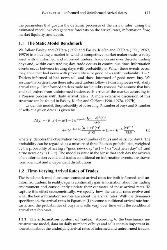
Table 4 Sample properties of the forecasts on proportion of informed trades (PIN).

Ticker Mean SD Auto Min Med Max

ASH 0.157 0.036 0.987 0.063 0.154 0.273XOM 0.121 0.025 0.951 0.045 0.114 0.213DUK 0.157 0.026 0.980 0.068 0.158 0.237ENE 0.149 0.036 0.992 0.065 0.145 0.286AOL 0.123 0.017 0.714 0.068 0.125 0.165MO 0.120 0.018 0.838 0.046 0.120 0.179T 0.110 0.012 0.831 0.053 0.109 0.161PFE 0.103 0.011 0.973 0.063 0.103 0.150LUV 0.187 0.043 0.988 0.073 0.187 0.302AMR 0.153 0.010 0.594 0.113 0.153 0.184DOW 0.103 0.011 0.808 0.056 0.103 0.158C 0.162 0.027 0.991 0.085 0.162 0.257JPM 0.140 0.017 0.838 0.058 0.141 0.198WMT 0.168 0.048 0.977 0.040 0.159 0.355HD 0.128 0.036 0.978 0.054 0.114 0.233GE 0.083 0.011 0.774 0.026 0.083 0.124

Entries report the sample average (Mean), standard deviation (SD), first-order autocorrelation (Auto),minimum (Min), median (Med), and maximum (Max) estimates on the forecasted time series of propor-tion of informed trades (PIN).

forecasts of the probability of informed trades, PIN. This conditional PIN is inter-preted as the forecast of the probability that a trade on the next day will be from aninformed agent. Then, we use these conditional PINs to predict market liquidity,exemplified by the opening bid-ask spread, using (14). The summary statistics forthe PIN forecasts are reported in Table 4.

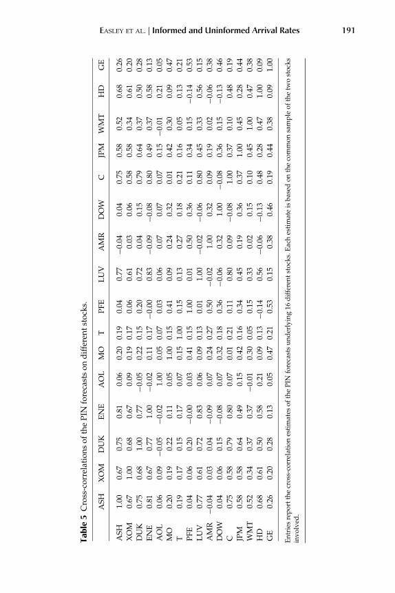
Figure 2 plots the time series of the PIN forecasts for each stock. For ease ofcomparison, we apply the same scale for all panels. We observe an obvious declinein the PIN forecasts over time for several stocks, especially during the last severalyears of our sample.

A new generation of asset pricing theories ascribe a role to liquidity. Easley,Hvidkjaer, and O’Hara (2002), O’Hara (2003), and Acharya and Pedersen (2005)differ on the measures of liquidity but agree on their importance. A simple measureof illiquidity is PIN, or the probability of informed trading. High values imply widebid-ask spreads, small market depths, and costly trading by uninformed traders.From Table 4 and Figure 2, it is clear that PIN varies across assets and over time.Although the average level of PIN is substantially different for these 16 stocks,perhaps even more important is the movement in this indicator. For each stock,the PIN estimate varies greatly over time. The minimum PIN estimates for moststocks are in single digits (in percentage points), but the maximum can well be over30 percentage points.


Tabl

e5

Cro

ss-c

orre

lati

ons

ofth

ePI

Nfo

reca

sts

ond

iffe

rent

stoc

ks.

ASH

XO

MD

UK

EN

EA

OL

MO

TPF

EL

UV

AM

RD

OW

CJP

MW

MT

HD

GE

ASH

1.00

0.67

0.75

0.81

0.06

0.20

0.19

0.04

0.77

−0.0

40.

040.

750.

580.

520.

680.

26X

OM

0.67

1.00

0.68

0.67

0.09

0.19

0.17

0.06

0.61

0.03

0.06

0.58

0.58

0.34

0.61

0.20

DU

K0.

750.

681.

000.

77−0

.05

0.22

0.15

0.20

0.72

0.04

0.15

0.79

0.64

0.37

0.50

0.28

EN

E0.

810.

670.

771.

00−0

.02

0.11

0.17

−0.0

00.

83−0

.09

−0.0

80.

800.

490.

370.

580.

13A

OL

0.06

0.09

−0.0

5−0

.02

1.00

0.05

0.07

0.03

0.06

0.07

0.07

0.07

0.15

−0.0

10.

210.

05M

O0.

200.

190.

220.

110.

051.

000.

150.

410.

090.

240.

320.

010.

420.

300.

090.

47T

0.19

0.17

0.15

0.17

0.07

0.15

1.00

0.15

0.13

0.27

0.18

0.21

0.16

0.05

0.13

0.21

PFE

0.04

0.06

0.20

−0.0

00.

030.

410.

151.

000.

010.

500.

360.

110.

340.

15−0

.14

0.53

LU

V0.

770.

610.

720.

830.

060.

090.

130.

011.

00−0

.02

−0.0

60.

800.

450.

330.

560.

15A

MR

−0.0

40.

030.

04−0

.09

0.07

0.24

0.27

0.50

−0.0

21.

000.

320.

090.

190.

02−0

.06

0.38

DO

W0.

040.

060.

15−0

.08

0.07

0.32

0.18

0.36

−0.0

60.

321.

00−0

.08

0.36

0.15

−0.1

30.

46C

0.75

0.58

0.79

0.80

0.07

0.01

0.21

0.11

0.80

0.09

−0.0

81.

000.

370.

100.

480.

19JP

M0.

580.

580.

640.

490.

150.

420.

160.

340.

450.

190.

360.

371.

000.

450.

280.

44W

MT

0.52

0.34

0.37

0.37

−0.0

10.

300.

050.

150.

330.

020.

150.

100.

451.

000.

470.

38H

D0.

680.

610.

500.

580.

210.

090.

13−0

.14

0.56

−0.0

6−0

.13

0.48

0.28

0.47

1.00

0.09

GE

0.26

0.20

0.28

0.13

0.05

0.47

0.21

0.53

0.15

0.38

0.46

0.19

0.44

0.38

0.09

1.00

Ent

ries

repo

rtth

ecr

oss-

corr

elat

ion

esti

mat

esof

the

PIN

fore

cast

sun

der

lyin

g16

dif

fere

ntst

ocks

.Eac

hes

tim

ate

isba

sed

onth

eco

mm

onsa

mpl

eof

the

two

stoc

ksin

volv

ed.


Figure 2 The time series of PIN forecasts. Lines depict the time series of the PIN forecasts fromour estimated dynamic model for each stock. PIN denotes the probability of informed trades,defined as the arrival of informed trades over the arrival of total trades. Each panel represents onestock. For ease of comparison, we apply the same scale on all panels.

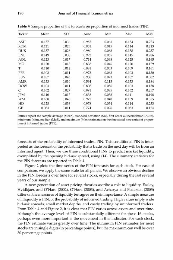
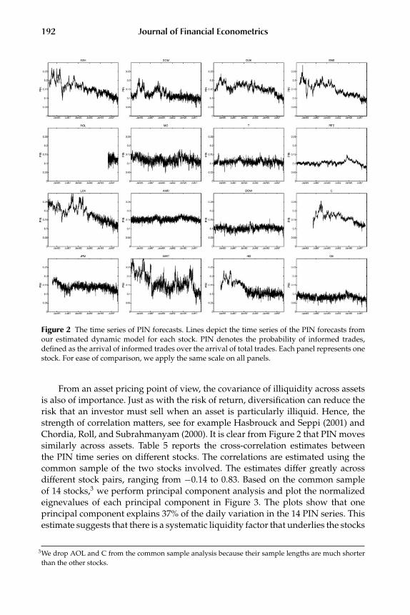
From an asset pricing point of view, the covariance of illiquidity across assetsis also of importance. Just as with the risk of return, diversification can reduce therisk that an investor must sell when an asset is particularly illiquid. Hence, thestrength of correlation matters, see for example Hasbrouck and Seppi (2001) andChordia, Roll, and Subrahmanyam (2000). It is clear from Figure 2 that PIN movessimilarly across assets. Table 5 reports the cross-correlation estimates betweenthe PIN time series on different stocks. The correlations are estimated using thecommon sample of the two stocks involved. The estimates differ greatly acrossdifferent stock pairs, ranging from −0.14 to 0.83. Based on the common sampleof 14 stocks,3 we perform principal component analysis and plot the normalizedeignevalues of each principal component in Figure 3. The plots show that oneprincipal component explains 37% of the daily variation in the 14 PIN series. Thisestimate suggests that there is a systematic liquidity factor that underlies the stocks

3We drop AOL and C from the common sample analysis because their sample lengths are much shorterthan the other stocks.


Figure 3 Percentage variation explained by each principal component of the PIN time series on14 stocks. The length of bars denotes the normalized eigenvalues of the covariance matrix of thedaily changes in the 14 time series of PIN estimates from our dynamic model. The normalizedeigenvalues can be interpreted as the percentage variation explained by each principal component.

that we estimate. While diversification can remove the idiosyncratic component ofthe liquidity risk, the systematic liquidity risk in each stock should be priced.

To examine how informative the arrival rate forecasts are in predicting theopening bid-ask spread, we run the following forecasting regression on each stock:

ln OPSt = c0 + c1 ln PINt−1 + c2 ln OPSt−1 + c3 GARCHt−1 + c4 ln Volumet−1 + et ,

(16)

where OPS denotes the percentage opening bid-ask spread of a stock, defined as

OPS ≡ 2ask − bidask + bid

, (17)

where we normalize the bid-ask spread by the average of the bid and ask level.The normalization has two purposes. First, we want to abstract from the impact ofthe scale of the quote. Second, we use the mid-quote as a proxy for the maximumimpact of the information event. The term PINt−1 denotes the time-(t − 1) forecastof the proportion of informed trades at time t. In addition to PIN, we also includethree control variables: (1) the lagged spread OPSt−1, (2) a standard GARCH(1,1)volatility estimate on the stock returns, GARCHt−1, which measures the time-(t − 1) forecast of time-t return volatility, and (3) the aggregate trading volumeat time (t − 1). We use these control variables to capture variations in the spreadthat are not explained by the proportion of informed trades. The first variablecaptures the unexplained persistence of the spread. The second variables capturesthe contribution of the price data, which can potentially reveal information aboutthe variation in the spread between the upper and lower bounds of the valuation


(V − V). The last variable captures the impact of trade size, which is absent fromour model. The significance of the estimates on c1 indicates how informative ourPIN forecasts are in predicting the opening bid-ask spread, on top of the predictionsfrom the three control variables.

Since the estimate for δ is not exactly at 1/2 for most stocks, in theory weshould use a more complicated function of arrival rates as in (14) rather thanPIN. Nevertheless, we use PIN for its simplicity and its intuitive interpretationas a measure for expected trade composition. Furthermore, several studies havegenerated the PIN estimates from the static model (based on either a rolling ora nonoverlapping window) and explored their implications. Using PIN from ourdynamic model provides a comparison with these studies.

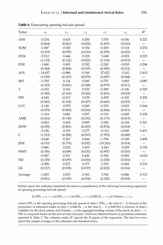
We estimate the regressions using generalized methods of moments, with theweighting matrix calculated according to Newey and West (1987) with 30 lags.Table 6 reports the slope estimates, their standard errors (in parentheses), andthe R-squares of the regressions in (16). The forecasting performance of the PINforecasts are quite remarkable. The estimates for the c1 coefficient, which capturesthe impact of the probability of informed trades, are significantly positive for all buttwo stocks. The sample average of c1 over the 16 stocks is 0.253, with an averagestandard deviation of 0.105. The strong statistical significance of the coefficientestimates are remarkable given that the arrival rate forecasts are obtained frompurely trade quantities while the opening bid-ask spread is a price behavior.

The c2 coefficient estimates on the autoregressive component are also signifi-cantly positive for all stocks, indicating that the persistence of the bid-ask spreadscannot be fully explained by the arrival rate forecasts. Furthermore, the coefficientestimates c3 on the GARCH volatility are on average positive and that on the trad-ing volume are on average negative, suggesting that the opening bid-ask spreadis higher if the previous day’s volatility is high but trading volume is low. Over-all, the regression in (16) exhibits pronounced forecasting power, with an averageR-square of 31.2%.

It is important to note that our arrival rates forecasts can be used to forecastthe bid-ask spreads under any given trade sequences. Here, we use the specificregressions on the opening bid-ask spreads to illustrate their forecasting powerand potential usefulness in forecasting the time-variation in market liquidity.

4.2 Market Depth and Price Impacts of Trade Orders

When a portfolio manager tries to purchase or liquidate a large position by sendingconsecutive buy or sell orders to the market, the price change induced by this seriesof orders could be significant. Using our dynamic microstructure framework, wecan compute the price impact of this sequence of orders as a function of the arrivalrates of informed and uninformed trades. Since we have forecasts of the arrivalrates, our dynamic model can also be used to forecast the market depth and thepotential cost of loading or unloading a position.

We use a sequence of N consecutive buy orders as an example. Let PrN−1t (good)

and PrN−1t (bad) denote the probabilities of a good and a bad information event


Table 6 Forecasting opening bid-ask spread.

Ticker c0 c1 c2 c3 c4 R2

ASH −3.234 0.625 0.200 3.576 −0.036 0.221(0.664) (0.061) (0.024) (2.453) (0.010) —

XOM −1.007 0.520 0.334 −0.205 −0.118 0.274(0.319) (0.059) (0.033) (0.399) (0.022) —

DUK −5.512 0.446 0.228 9.648 −0.018 0.229(1.133) (0.122) (0.025) (3.118) (0.013) —

ENE −1.860 0.405 0.352 −2.245 −0.010 0.206(0.364) (0.068) (0.035) (0.950) (0.012) —

AOL −14.457 −0.886 0.344 27.622 0.162 0.410(1.539) (0.167) (0.079) (2.697) (0.044) —

MO −3.705 0.124 0.285 −0.751 0.003 0.085(0.323) (0.061) (0.028) (0.579) (0.011) —

T −0.232 0.341 0.522 −0.289 −0.106 0.325(0.349) (0.103) (0.026) (0.451) (0.018) —

PFE −4.942 −0.215 0.238 6.878 −0.105 0.292(0.441) (0.102) (0.027) (0.662) (0.015) —

LUV −2.140 0.578 0.269 −0.239 −0.019 0.264(0.278) (0.069) (0.026) (0.848) (0.011) —

−1.314 0.082 0.557 −0.119 −0.068 0.339AMR (0.416) (0.138) (0.032) (0.173) (0.013) —

−0.063 0.418 0.499 0.383 −0.144 0.321DOW (0.259) (0.081) (0.025) (0.874) (0.018) —

−5.156 0.335 0.277 11.511 −0.045 0.491C (1.515) (0.289) (0.053) (1.970) (0.049) —

−0.648 0.267 0.444 −1.784 −0.108 0.400JPM (4.531) (0.170) (0.032) (19.243) (0.014) —

−3.886 0.210 0.453 4.243 0.029 0.318WMT (0.356) (0.049) (0.033) (0.987) (0.010) —

−0.587 0.531 0.420 −0.302 −0.093 0.610HD (0.329) (0.059) (0.030) (1.020) (0.010) —

−2.508 0.273 0.377 2.333 −0.065 0.214GE (0.317) (0.078) (0.037) (0.822) (0.016) —

Average −3.203 0.253 0.363 3.766 −0.046 0.312(0.821) (0.105) (0.034) (2.328) (0.018) —

Entries report the estimates (standard deviation in parentheses) of the following forecasting regressionon opening percentage bid-ask spread:

ln OPSt = c0 + c1 ln PINt−1 + c2 ln OPSt−1 + c3 GARCHt−1 + c4 ln Volumet−1 + et ,

where OPSt is the opening percentage bid-ask spread at date t, PINt−1 the time-(t − 1) forecast of theproportion of informed trades at time t, GARCHt−1 is the time-(t − 1) GARCH(1,1) forecast of time-tvolatility for the stock return, and Volumet−1 is the aggregate trading volume of the stock on date t − 1.PIN is computed based on the arrival rates forecasts, which are obtained based on parameter estimatesreported in Table 2. The columns under R2 reports the R-square of the regression. The last two rowsreport the sample averages of the estimates and standard errors.


Figure 4 The price impact of consecutive buy orders on Ashland Oil. The lines depict the normal-ized price impact curves of consecutive buys (γ N

t /δ), computed based on the arrival rate forecastson Ashland Oil from our dynamic model on three different dates, when the forecasted proportionof informed trades (PIN) is at the minimum (left panel), median (middle panel), and maximum(right panel), respectively.

conditional on N − 1 consecutive buy orders. From (12), we can derive the priceimpact of N consecutive buys as

askNt = V∗ + (V − V)γ N

t ,

where γ Nt captures the impact of N consecutive buys:

γ Nt = δ PrN−1

t (good)(εt−1 + µt−1) − (1 − δ) PrN−1t (bad)εt−1

PrN−1t (good)µt−1 + εt−1

. (18)

The probabilities PrN−1t (good) and PrN−1

t (bad) can be readily updated via Bayesrule as in (11), starting from the unconditional priors at the opening. As the numberof consecutive buy orders increases, the probability of a good information eventincreases and approaches unity while the probability of a bad information eventapproaches zero. The price impact γ N

t converges to δ, and the price converges tothe expected upper bound of the asset value V. The speed of convergence governsthe depth of the market and is determined by the arrival rate forecasts (µt−1, εt−1).

To illustrate how the arrival rate forecasts impact the market depth, we usethe first stock of our sample, Ashland Oil, as an example and consider three datesin our sample period when the PIN forecasts on Ashland are at the sample mini-mum, median, and maximum, respectively. At each of three PIN levels, we use theestimated model parameters on Ashland Oil and the arrival rate forecasts for thatdate to compute the price impacts of N consecutive buy orders (γ N

t ) according toEquation (18) and then normalize the impacts by their convergent value δ. Figure 4plots the three normalized price impact curves (γ N

t /δ) as a function of the numberof consecutive buy orders (N) at the three selected PIN levels for Ashland.

All three normalized curves start at zero with zero trade and converge toone as the stock price converges to its upper bound V with increasing number ofconsecutive buy orders. The speeds of convergence are captured by the slope of thecurves and are different under different arrival rate forecasts. During the sampleperiod, the minimum forecasted PIN for Ashland is 6.34%. Under this minimumlevel of forecasted informed trading (left panel), the market maker adjusts the askquote slowly to the order flow. It takes about 30 consecutive buy orders for the stock


price to converge to its upper bound. The market is therefore deep. In contrast, themaximum PIN forecast for Ashland is 27.27%. At this maximum level of forecastedinformed trading (right panel), the market makers adjusts the ask price quickly tothe sequence of buy orders. The price converges to its upper bound after fewer than10 consecutive buy orders. The middle panel in Figure 4 shows an intermediateprice impact curve when the forecasted proportion of arrival rates are at the medianlevel of 15.37%.

Given the estimated model parameters and the arrival rate forecasts, we canalso compute the price impact curve for N consecutive sells and for any sequenceof buys and sells. Knowledge of the price impact curve is very important forinstitutional portfolio managers in analyzing the potential trading cost and indesigning strategies for loading or unloading their positions. Our arrival rateforecasts can be used to predict the market depth and trading cost in terms of suchprice impact curves.

The price impact curve of a sequence of order flows provides the completepicture on the market depth, but it is often useful to summarize the market depthwith a more compact measure. For example, Engle and Lange (2001) define amarket depth measure VNET, which is designed to capture the net order flowassociated with a fixed price movement. The larger this net order flow is for a fixedprice movement, the deeper the market is. Based on the arrival rate forecasts, weconstruct an analogous measure of market depth: the half-life (τ1/2) of the priceimpacts for consecutive buys. Our measure is defined as the number of buys Nneeded for the normalized price impact γ N

t /δ to exceed half of its maximum impact.Intuitively, the half-life measure provides the portfolio managers an estimate onthe maximum number of buy orders he can execute for the price impact to staywithin a certain range.

Our half-life measure and VNET differ in at least two important aspects. First,VNET is defined on the excess trading volume while we are only concerned withthe net number of trades. Trade size does not play a role in our analysis. A seconddifference is that VNET implicitly assumes that the sequence of trades does notmatter, only the net trade imbalance affects prices. In our model, however, the exactsequence of trading history also plays an important role in the price movement. Wetherefore specifically define the half-life as a function of the number of consecutivebuys, not net order flows.

Figure 5 depicts three typical time series of our market depth (half-life) fore-casts for, from left to right, Ashlan, Exxon Mobil, and General Electric, respectively.For all three stocks, the market depth measured by half-life has increased in thenineties.

4.3 Informed Arrivals Before and After Earnings Announcements

We specify the arrival rates of informed and uninformed trades as a vector au-toregressive process, in which balanced and imbalanced trades act as noisy signalsabout the underlying arrival rates. The arrival of informed trades is jointly deter-mined by the arrival of traders and the arrival of information. Large informational


Figure 5 Time-varying forecasts of market depth. Lines depict three typical time series on thehalf-life (τ1/2) of the price impact of consecutive buy orders, defined as the number of consecutivebuys needed for the impact to exceed half of its maximum. The half-life is computed based onour estimated dynamic model for, from left to right, Ashland, Exxon Mobil, and General Electric,respectively.

events, such as the releases of important economic numbers and the announce-ment of corporate earnings, happen at predetermined calendar dates, generatingcalendar days effects in the information flow and in the arrival rate of informedtrades.

To study whether our arrival rate estimates capture some of the calendar dayeffects, we take corporate earnings announcements as an example and performan event study around announcement days. Specifically, we compute the aver-age PIN estimates as a function of the number of business days before and afterthe earning announcement days for each company. We obtain the announcementdates from the CompuStat. During our sample period, there are altogether 834earnings announcements for the 16 stocks. Among them, 124 happened on Mon-days, 183 happened on Tuesdays, 190 happened on Wednesdays, 229 happenedon Thursdays, and 108 happened on Fridays. We do not know the exact timing ofthe announcement. Since the announcement can happen before the open, after theclose, or during the trading hours, our measure of the number of business daysbefore and after the announcement can deviate from the true measure by one day.

The left panel of Figure 6 plots the average PIN estimates as a function ofthe number of business days before and after the earning announcement date.The solid line denotes the sample average. The two dash-dotted lines representthe one standard deviation bands on the mean estimates. The plot shows that theproportion of informed trades increases as the announcement date approaches anddeclines after the announcement. The variation is the most significant within a ±7business day window.

For comparison, we also compute the average proportion of imbalanced trades,defined as |B − S|/(B + S). If the order imbalances reveal the informed arrivalwith little noise, we would expect to observe similar average patterns. Figure 6plots the results on the proportion of imbalanced trades in the right panel. Theaverage proportions of imbalanced trades are higher than the average proportionof informed trade arrivals, potentially indicating that the imbalanced trades containmore noise than the balanced trades about the underlying arrival rates. The averageestimates of the proportion of imbalanced trades show large zig-zag variationsacross different days, with little identifiable systematic patterns. Comparing the


Figure 6 Proportion of informed arrivals and imbalanced trades before and after earnings an-nouncements. The left panel plots the average proportion of informed trade arrival rates as afunction of number of days before and after the earning announcement dates. The right panelplots the proportion of imbalanced trades. In both panels, the solid lines denote the sample aver-age over the 834 earning announcement events across the 16 stocks. The dash-dotted lines definea one-standard deviation band.

scales of the two panels reveals that the large noise-induced zig-zag variation in theright panel completely dominates the systematic pattern observed in the left panel.The difference between the highest average PIN estimate at the announcement dayand the lowest PIN estimate at seven days after the announcement is 56 basis points.By contract, the zig-zag pattern in the right panel generates differences betweenneighboring estimates as high as 153 basis points. Thus, the systematic informationabout informed and uninformed arrivals is completely buried in the large noise ofthe raw order flow numbers. The different results from the two panels highlightthe virtue of our dynamic specification in extracting useful information from thehighly noisy realizations.

In a working paper, Benos and Jochec (2007) divide each quarter in betweenthe earnings announcement days into two subsample periods. Then, they estimatethe constant arrival rates in the static model separately for the two periods. Theycompute the PIN from the two sets of estimates and find that the average PINestimate is lower before the announcement than after the announcement period.Our result shows that the PIN variation around the announcement dates happenwithin a very narrow window of ±7 days before and after the announcement.Thus estimation based on the static model using one and a half-month window isunlikely to reveal actual announcement day effects.

Several other studies have estimated the PIN measure assuming that the arrivalrates of informed and uninformed trades are constant over time. Examples includeEasley, Kiefer, and O’Hara (1996), Easley et al. (1996), Easley, O’Hara, and Paperman(1998), Easley, Hvidkjaer, and O’Hara (2002, 2005), Dennis and Weston (2001),Easley, O’Hara, and Saar (2001), Vega (2005). To accommodate the time variation ofthe arrival rates in reality, they resort to repeated calibration over different sampleperiods. The re-calibration is often performed on a quarterly or annual frequency.In this paper, by specifying a dynamic process for the arrival rates, we can capture


the daily time variation of the arrival rates, and we can do so consistently with amodel that is estimated only once over the whole sample period. Our analysis inthis section further shows that capturing the daily variation in the arrival rates canbe important in, for example, predicting opening bid-ask spreads and revealingannouncement day effects.

5 DIAGNOSTIC ANALYSIS

By blending a microstructure framework with a dynamic forecasting specification,we can infer and predict the unobservable arrival rates of informed and uninformedtrades based on the observable order flow of buys and sells. Our analysis so farhas shown the great promise of using the arrival rate forecasts to predict bid-askspreads and the price impact of a sequence of order flows, both of which aredetermining factors for trading cost analysis.

The accuracy of the arrival rate forecasts depends both on the microstruc-ture setup and on the dynamic forecasting specification. The microstructure setupdetermines the likelihood of a sequence of buys and sells whereas the dynamicspecification dictates the dynamics of the arrival rates. In this section, we performdiagnostic analysis on our dynamic microstructure model.

Based on the forecasted arrival rates of informed and uninformed trades, weforecast balanced and imbalanced trades. Therefore, one way to investigate therobustness of our specification is to check for remaining structure in the residualsof these trade forecasts. If our specification captures the data well, we shouldfind minimal structure from the following standardized forecasting residuals et ≡[e1t , e2t]�:

eit = Zi t − Et−1[Zi t]√Vart−1[Zi t]

, i = 1, 2, with Zt = [|Kt|, TTt − |Kt|].

If the model is specified correctly, each of the two standardized forecasting residualseit should be serially independent and should have zero mean and unit variance.The number of buys and sells is governed by mixtures of Poisson distributions asshown in Equation (5). We can readily compute the conditional mean and varianceof the trade quantities Zt by simulation.

Table 7 reports the summary statistics for the residuals. For each stock, thefirst row reports the properties of the standardized residual on the absolute tradeimbalance and the second row reports the properties of the standardized residualon the balanced trades. Compared to the summary statistics of the raw tradequantities Z in Table 1, the forecasting residuals show much less structure. Thesample averages of the residuals are very close to zero. The serial dependence (thefirst-order autocorrelation) is significantly smaller than that in the raw series, andin many cases are no longer significantly different from zero. The cross-correlationsbetween the two residuals are also smaller than those between the two elementsof the raw trade quantities.

Nevertheless, we can still discern some remaining structure in the residuals.For example, the standard deviation of the standardized residual of the balanced


Table 7 Summary statistics of the standardized forecasting residuals.

Ticker Mean SD Auto VR ρ

ASH −0.022 0.996 0.014 0.157 −0.1110.008 1.872 0.026 0.693 —

XOM 0.176 1.208 0.206 0.182 −0.354−0.100 2.934 0.064 0.844 —

DUK 0.073 1.179 0.090 0.184 −0.275−0.069 1.845 0.007 0.807 —

ENE 0.044 1.074 0.050 0.254 −0.186−0.024 2.081 0.025 0.837 —

AOL 0.215 1.084 −0.005 0.500 0.2330.028 6.108 0.104 0.832 —

MO 0.000 1.028 0.145 0.317 −0.026−0.101 4.122 0.096 0.865 —

T 0.204 1.182 0.280 0.140 −0.192−0.275 3.837 0.097 0.728 —

PFE 0.204 1.076 0.179 0.239 −0.033−0.098 3.439 0.095 0.919 —

LUV −0.124 0.880 0.096 0.342 −0.036−0.066 2.584 0.057 0.830 —

AMR −0.220 0.887 0.028 0.564 0.0580.057 3.233 0.042 0.703 —

DOW 0.012 1.001 0.152 0.093 −0.1100.018 2.825 0.047 0.573 —

C 0.441 0.896 0.089 0.200 0.068−0.337 4.527 0.205 0.773 —

JPM −0.025 1.038 0.085 0.387 −0.076−0.014 2.707 0.072 0.830 —

WMT 0.085 1.156 0.187 0.237 −0.236−0.177 3.132 0.089 0.867 —

HD 0.317 1.115 0.285 0.135 −0.089−0.142 3.417 0.121 0.825 —

GE 0.103 1.074 0.111 0.415 −0.1380.029 3.513 0.083 0.893 —

Average 0.093 1.055 0.124 0.272 −0.094−0.079 3.261 0.077 0.801 —

Entries report the summary statistics of standardized forecasting residuals on the absolute trade imbal-ance |K | and the balanced trade TT − |K |:

eit = Zi t − Et−1[Zi t]√Vart−1[Zi t]

, i = 1, 2, with Zt = [|Kt |, TTt − |Kt |].

“Mean” is the sample average, “SD” is the standard deviation, “Auto” is the first-order autocorrelation,“VR” is the ratio of the variance of the forecasted trade quantity Et−1[Zi t] versus the variance of therealized quantity Zt , VR = Var (Et−1[Zi t])/Var (Zi t), and “ρ” denotes the cross-correlation coefficientbetween the two residuals. For each stock, the first row reports the properties of the residual on absolutetrade imbalance and the second row reports the properties of the residual on balanced trade. The lasttwo rows report the sample averages of the statistics across the 16 stocks.


trade is systematically greater than one for all stocks. We conjecture that the biasis induced by the Poisson arrival assumptions on the informed and uninformedtraders. A Poisson distribution is natural and tractable for modeling the arrivalof traders, but a key limitation of this assumption is that the mean and varianceof a Poisson variable are controlled by a single parameter—the Poisson arrivalrate. The biases in the residuals of the balanced trades seem to indicate that theobserved distribution of the balanced trades is more dispersed than implied by themixture of Poisson distributions. If our conjecture is correct, the observed biases inthe forecasting residuals can be corrected by choosing a more flexible distributionfor the arrival of informed and uninformed traders so that we can disentangle themean and variance of the trade quantities.

To gauge the forecasting power of our dynamic systems, we also report thepercentage of variance (VR) in the two trade quantities explained by our model.The percentage variance VR is defined as the ratio of the variance of the forecastedtrade quantities over the variance of the realized trade quantities. Overall, themodel explains a larger percentage of the variation in the balanced trades thanfor the trade imbalance. This is not surprising given the inherent difficulty inforecasting informed arrivals.

As a test on our forecasting dynamics specification, we investigate whetherthe standardized residuals eit can be forecasted further by additional variables:

eit = c0 + c1 Zi(t−1) + c2 GARCHt−1 + c3 ln Volumet−1 + ηi t , (19)

where Zi(t−1) denotes the time-(t − 1) autoregressive forecasts of Zit , GARCHt−1

denotes the time-(t − 1) GARCH(1,1) forecasts of the stock return volatility, andVolumet−1 is the time-(t − 1) aggregate trading volume of the stock. In this regres-sion, we use the first variable to capture the persistence of the order flows thatis missed by our dynamic specification in Equation (4). Furthermore, we use theGARCH volatility to capture the information from the price data, and the tradingvolume to capture the information in the trade size, neither of which is accom-modated in our forecasting specification in Equation (4). A significant estimate onc1 would point to further room for improvement in our dynamics specification.Significant estimates on c2 and c3 would show that price and trade size informa-tion can also be embedded in the forecasting dynamics for the arrival rates. Asin GARCH-type models, the forecasting dynamics specification in Equation (2)can readily be extended to accommodate additional observables as long as theyare informative about the unobservable arrival rates. Thus, a diagnostic regressionlike this can be used to identify additional informational sources for the predictionof the informed and uninformed arrival rates.

We estimate Equation (19) using the generalized methods of moments, wherethe weighting matrix is calculated according to Newey and West (1987) with 30lags. Furthermore, to control the scale of the slope coefficients, we standardizeeach regressor by subtracting its sample mean and further scaling it by its samplestandard deviation. Table 8 reports the coefficient estimates and standard errors.The last column under R2 reports the R-square of the regression. For each stock, the


Table 8 Regressing the standardized forecasting residuals on additional variables.

Ticker c0 c1 c2 c3 R2

ASH −0.022 (0.020) 0.006 (0.018) −0.025 (0.016) −0.033 (0.022) 0.0020.007 (0.029) 0.064 (0.055) 0.025 (0.030) 0.038 (0.039) 0.002

XOM 0.176 (0.041) 0.217 (0.033) −0.018 (0.019) −0.193 (0.030) 0.050−0.103 (0.049) 0.095 (0.076) −0.036 (0.042) −0.012 (0.070) 0.001

DUK 0.073 (0.030) 0.086 (0.025) 0.117 (0.030) −0.035 (0.023) 0.015−0.070 (0.028) 0.041 (0.062) 0.011 (0.041) 0.051 (0.038) 0.002

ENE 0.044 (0.029) 0.071 (0.030) 0.003 (0.031) −0.093 (0.034) 0.007−0.028 (0.035) 0.004 (0.081) −0.007 (0.052) 0.095 (0.058) 0.002

AOL 0.209 (0.064) −0.042 (0.066) −0.275 (0.044) −0.252 (0.057) 0.0430.008 (0.246) 0.819 (0.595) −0.361 (0.421) −1.041 (0.463) 0.011

MO −0.001 (0.026) 0.227 (0.022) −0.015 (0.014) −0.154 (0.026) 0.039−0.107 (0.060) 0.023 (0.143) 0.028 (0.055) −0.042 (0.122) 0.000

T 0.203 (0.039) 0.302 (0.028) 0.021 (0.021) −0.122 (0.031) 0.059−0.276 (0.061) 0.256 (0.094) 0.125 (0.056) −0.170 (0.090) 0.003

PFE 0.202 (0.027) 0.271 (0.028) 0.107 (0.030) −0.068 (0.031) 0.041−0.099 (0.058) −0.000 (0.187) −0.163 (0.134) −0.091 (0.099) 0.001

LUV −0.124 (0.021) 0.105 (0.024) 0.010 (0.014) 0.025 (0.019) 0.019−0.068 (0.040) −0.037 (0.071) −0.042 (0.038) 0.066 (0.061) 0.001

AMR −0.220 (0.022) 0.012 (0.020) −0.002 (0.013) −0.075 (0.017) 0.0060.055 (0.048) 0.176 (0.088) −0.015 (0.040) −0.062 (0.071) 0.002

DOW 0.012 (0.022) 0.200 (0.041) 0.001 (0.014) −0.136 (0.020) 0.0480.019 (0.047) 0.004 (0.071) 0.040 (0.038) 0.058 (0.063) 0.001

C 0.437 (0.053) 0.140 (0.041) −0.053 (0.068) −0.094 (0.050) 0.020−0.347 (0.170) 1.291 (0.364) 1.005 (0.473) −0.165 (0.544) 0.032

JPM −0.026 (0.029) 0.087 (0.022) −0.005 (0.015) −0.103 (0.027) 0.010−0.014 (0.050) 0.086 (0.072) 0.018 (0.034) 0.023 (0.058) 0.001

WMT 0.079 (0.029) 0.206 (0.023) 0.095 (0.028) 0.015 (0.037) 0.036−0.183 (0.043) 0.060 (0.097) −0.097 (0.056) −0.064 (0.070) 0.001

HD 0.315 (0.031) 0.374 (0.041) 0.051 (0.029) −0.020 (0.030) 0.100−0.148 (0.062) 0.266 (0.105) 0.134 (0.077) −0.057 (0.093) 0.003

GE 0.098 (0.029) 0.150 (0.035) 0.025 (0.022) −0.186 (0.026) 0.0310.026 (0.053) 0.145 (0.154) 0.078 (0.064) 0.025 (0.105) 0.002

Average 0.091 (0.032) 0.151 (0.031) 0.002 (0.025) −0.095 (0.030) 0.033−0.083 (0.067) 0.206 (0.145) 0.046 (0.103) −0.084 (0.128) 0.004

Entries report the estimates and standard deviations of the following regression on the standardizedforecasting residuals:

eit = c0 + c1 Zi(t−1) + c2 GARCHt−1 + c3 ln Volumet−1 + ηi t ,

where Zi(t−1) denotes the autoregressive forecasts on Zit GARCHt−1 is the GARCH(1,1) volatility estimatefrom the stock returns, and Volumet−1 is the aggregate trading volume of the stock on date t − 1. Westandardize each regressor by subtracting its sample mean and further scaling it by its sample standarddeviation. The column under R2 reports the R-square of the regression. For each stock, the first row reportsthe properties of the residual on absolute trade imbalance and the second row reports the properties ofthe residual on balanced trade. The last two rows report the sample averages of the statistics across the16 stocks.


first row reports the regression for the residual on absolute trade imbalance andthe second row reports that for the residual on balanced trade. The last two rowsreport the sample average of the statistics across the 16 stocks. The R-squares ofthese regressions are very small, with an average of 3.3% for the imbalanced traderesidual and an average of 0.4% for the balanced trade. The small R-squares suggestthat the three additional variables add little to the forecasting of the order flows. In-specting the slope coefficient estimates, we find that on average, the autoregressiveforecast of the trade imbalance predicts positively and the trading volume predictsnegatively on the trade imbalance residual. On the other hand, none of the threevariables add significantly to the prediction of the balanced trades. On average,the intercept of the balanced residual is not statistically different from zero, either.

6 CONCLUSION

In this paper, we model the dynamics of trade arrivals in the context of the Easleyand O’Hara (1992) microstructure model. We select a sample of 16 actively tradedNYSE stocks and use 15 years of daily transaction data to illustrate how we canestimate the arrival dynamics of trades originating from informed and uninformedtraders using the daily number of buys and sells for each stock. The model is formu-lated as a point process for each type of investor where the parameter measuringthe trade intensity is conditional on past information. These conditional intensitiesare modeled as functions of past balanced and unbalanced trades allowing for timetrends and dynamic interactions.

The most immediate conclusion is our finding of strong daily autocorrelationsin all of the trade series. Not only are trades in each stock strongly autocorrelated,but the number of balanced trades is highly autocorrelated and the number ofunbalanced trades is weakly autocorrelated. As a consequence, the model impliesthat the arrival rate of uninformed trades is highly autocorrelated but that ofinformed traders is less so. Of particular interest is the observation that the arrivalrate of uninformed trades is negatively affected by the past conditional arrivalrates of informed trades. We conclude from this evidence that uninformed tradersattempt to time their trades to avoid informed traders.

A further intriguing observation is in the dynamics of the informed traders.They show only a weak response to the conditional intensity of uninformed traders,even though they could be expected to hide in the crowd of uninformed trading.This is a natural finding in models with competing informed traders who willtrade until profit is extracted from prices and then stop. Thus we conclude that itis the presence of information, rather than variation in the intensity of uninformedtrade, that determines the arrival rate of informed traders.

We also show how these insights into the behavior of informed and uninformedtraders can be used to predict other characteristics of the market. We calculateforecasts of measures of liquidity such as bid-ask spreads and market depth fromthe model estimates. We show that these forecasts are informative in predictingvariations in market liquidity. We also use our dynamic model to generate a timeseries of the probability of information-based trade (PIN). We show how to use


this time series of PINs to investigate the effects of earnings announcements on thevariation in information-based trading.

There are many potential applications for the market liquidity and depthforecasts that our dynamic microstructure model generates. From the academicperspective, understanding the evolution of liquidity and its interaction with in-formation flow provides insight into the price formation process as well as intothe more general area of asset pricing. For example, Easley, Hvidkjaer, and O’Hara(2002) use a static version of PIN forecasts to analyze whether information risk ispriced. Using our dynamic model should provide a more consistent analysis be-tween the estimated dynamics underlying the PIN forecasts and the cross-sectionalpatterns in stock returns. Most recently, Acharya and Pedersen (2005) develop anequilibrium asset pricing model with liquidity risk. They show that a security’srequired return depends on its expected liquidity as well as on the covariances ofits own return and liquidity with market return and liquidity. Our dynamic arrivalrate specifications provide evidence on how liquidity risk evolves over time andon its correlations across assets. We believe that our approach should provide avaluable starting point for further tests of the asset pricing implications of dynamicliquidity and a deeper understanding of the origins of liquidity correlations.

From a practical perspective, our model-based market liquidity and depth fore-casts should be useful for trading cost analysis, which has emerged as a valuabletool to help portfolio managers handle execution costs in implementing their trad-ing strategies. With performance typically benchmarked to some index, whethera manager is able to outperform is ever more determined by the skill with whichhe executes trades. Our dynamic microstructure model allows richer forecasts oftrading cost from hypothetical trade sequences and should be useful in allowingtraders to select strategies to minimize these costs.

Finally, from a risk management point of view, our estimates provide aforward-looking estimate of the sources of liquidation costs of a portfolio posi-tion. This should prove a useful input to calculation of the “liquidity risk” of aportfolio.

Received October 24, 2006; revised January 7, 2008; accepted January 10, 2008.

REFERENCES

Acharya, V. V., and L. H. Pedersen. (2005). “Asset Pricing with Liquidity Risk.” Journalof Financial Economics 77(2), 375–410.

Admati, A. R., and P. Pfleiderer. (1988). “A Theory of Intraday Patterns: Volume andPrice Variability.” Review of Financial Studies 1(1), 3–40.

Benos, E., and M. Jochec. (2007). “Testing the PIN Variable.” Working paper, Universityof Illinois at Urbana-Champaign, IL.

Bollerslev, T. (1986). “Generalized Autoregressive Conditional Heteroskedasticity.”Journal of Econometrics 31, 307–327.

Chordia, T., R. Roll, and A. Subrahmanyam. (2000). “Commonality in Liquidity.” Journalof Financial Eonomics 56(1), 3–28.


Chordia, T., R. Roll, and A. Subrahmanyam. (2001a). “Market Liquidity and TradingActivity.” Journal of Finance 56(2), 501–530.

Chordia, T., R. Roll, and A. Subrahmanyam. (2001b). “Trading Activity and ExpectedStock Returns.” Journal of Financial Economics 59(1), 3–28.

Chordia, T., R. Roll, and A. Subrahmanyam. (2002). “Order Imbalance, Liquidity, andMarket Returns.” Journal of Financial Economics 65(1), 111–130.

Chordia, T., R. Roll, and A. Subrahmanyam. (2005). “Evidence on the Speed of Conver-gence to Market Efficiency.” Journal of Financial Economics 76(2), 271–292.

Chordia, T., and A. Subrahmanyam. (2004). “Order Imbalance and Individual StockReturns: Theory and Evidence.” Journal of Financial Economics 72(3), 485–518.

Dennis, P. J., and J. Weston. (2001). “Who Is Informed? An Analysis of Stock Ownershipand Informed Trading.” Working paper, University of Virginia and Rice University.

Dufour, A., and R. F. Engle. (2000). “Time and the Price Impact of a Trade.” Journal ofFinance 55(6), 2467–2598.

Easley, D., S. Hvidkjaer, and M. O’Hara. (2002). “Is Information Risk a Determinant ofAsset Returns?” Journal of Finance 57(5), 2185–2221.

Easley, D., S. Hvidkjaer, and M. O’Hara. (2005). “Factoring Information into Returns.”Working paper, Cornell University and University of Maryland.

Easley, D., N. M. Kiefer, and M. O’Hara. (1996). “Cream-Skimming or Profit-Sharing?The Curious Role of Purchased Order Flow.” Journal of Finance 51(3), 811–833.

Easley, D., N. M. Kiefer, and M. O’Hara. (1997a). “The Information Content of TheTrading Process.” Journal of Empirical Finance 4(2–3), 159–185.

Easley, D., N. M. Kiefer, and M. O’Hara. (1997b). “One Day in the Life of a Very CommonStock.” Review of Financial Studies 10(3), 805–835.

Easley, D., N. M. Kiefer, M. O’Hara, and J. B. Paperman. (1996). “Liquidity, Information,and Infrequently Traded Stocks.” Journal of Finance 51(4), 1405–1436.

Easley, D., and M. O’Hara. (1992). “Time and the Process of Security Price Adjustment.”Journal of Finance 47(2), 577–605.

Easley, D., M. O’Hara, and J. Paperman. (1998). “Financial Analysts and Information-Based Trade.” Journal of Financial Markets 1(2), 175–201.

Easley, D., M. O’Hara, and G. Saar. (2001) “How Stock Splits Affect Trading: A Mi-crostructure Approach.” Journal of Financial and Quantitative Analysis 36(1), 25–51.

Engle, R. F. (2000). “The Econometrics of Ultra High Frequency Data.” Econometrica68(1), 1–22.

Engle, R. F., and J. Lange. (2001). “Predicting VNET: A Model of the Dynamics of MarketDepth.” Manuscript, New York University and Federal Reserve Board.

Engle, R. F., and J. R. Russell. (1998). “Autoregressive Conditional Duration: A NewModel for Irregularly Spaced Transaction Data.” Econometrica 66(5), 1127–1162.

Foster, D., and S. Vishwanathan. (1990). “A Theory of the Intraday Variations in Volume,Variance, and Trading Costs in Securities Markets.” Review of Financial Studies 3(4),593–624.

Hasbrouck, J. 1991. “Measuring the Information Content of Stock Trades.” Journal ofFinance 46(1), 179–208.

Hasbrouck, J., and D. J. Seppi. (2001). “Common Factors in Prices, Order Flows, andLiquidity.” Journal of Financial Eonomics 59(3), 383–411.


Katti, S. K. (1960). “Moments of Absolute Difference and Absolute Deviation of DiscreteDistributions.” Annals of Mathematical Statistics 31(1), 78–85.

Korajczyk, R. A., and R. Sadka. (2006). “Pricing the Commonality Across AlternativeMeasures of Liquidity.” Working paper, Northwestern University.

Lee, C. M. C., and M. A. Ready. (1991). “Inferring Trade Direction from Intraday Data.”Journal of Finance 46(2), 733–746.

Lei, Q., and G. Wu. (2000). “The Behavior of Uninformed Investors and Time-VaryingInformed Trading Activities.” Manuscript, University of Michigan.

Manganelli, S. (2000). “Time, Volume and Price Impact of Trades.” Manuscript, Euro-pean Central Bank, Germany.

Nelson, D. B. (1991). “Conditional Heteroskedasticity in Asset Returns: A New Ap-proach.” Econometrica 59(2), 347–370.

Newey, W. K., and K. D. West. (1987). “A Simple, Positive Semi-Definite, Heteroskedas-ticity and Autocorrelation Consistent Covariance Matrix.” Econometrica 55(3), 703–708.

O’Hara, M. (2003). “Presidential Address: Liquidity and Price Discovery.” Journal ofFinance 58(4), 1335–1354.

Vega, C. (2005). “Stock Price Reaction to Public and Private Information.” Journal ofFinancial Economics 82(1), 103–133.

Documents

Time-Varying Arrival Rates of Informed and …pages.stern.nyu.edu › ~rengle › EngleEasleyOharaWu.pdfJournal of Financial Econometrics, 2008, 171–207 Time-Varying Arrival Rates