Timed-automata abstraction of switcheddynamical systems using control invariants?

Patricia Bouyer1, Nicolas Markey1,Nicolas Perrin2,3, Philipp Schlehuber-Caissier2

1LSV – CNRS & ENS Cachan – Universite Paris-Saclay – France2Sorbonne Universites, UPMC Univ Paris 06, UMR 7222, ISIR, F-75005, Paris, France

3CNRS, UMR 7222, ISIR, F-75005, Paris, France

Abstract. The development of formal methods for control design is animportant challenge with potential applications in a wide range of safety-critical cyber-physical systems. Focusing on switched dynamical systems,we propose a new abstraction, based on time-varying regions of invariance(control funnels), that models behaviors of systems as timed automata.The main advantage of this method is that it allows for the automatedverification and reactive controller synthesis without discretizing theevolution of the state of the system. Efficient and analytic constructionsare possible in the case of linear dynamics whereas bounding funnelswith conjectured properties based on numerical simulations can be usedfor general nonlinear dynamics. We demonstrate the potential of ourapproach with three examples.

1 Introduction

Verification and synthesis are notoriously difficult for hybrid dynamical systems,i.e. systems that allow abrupt changes in continuous dynamics. For instance,reachability is already undecidable for 2-dimensional piecewise-affine maps [16],or for 3-dimensional dynamical systems with piecewise-constant derivatives [2].

To enable automated logical reasoning on switched dynamical systems, mostmethods tend to entirely discretize the dynamics, for example by approximatingthe behavior of the system with a finite-state machine. Alternatively, early workpointed out links between hybrid and timed systems [22], and several methods havebeen designed to create formal abstractions of dynamical systems that do not relyon a discretization of time. In [13], a finite maneuver automaton is constructedfrom a library of motion primitives, and motion plans correspond to timedwords. In [18, 14], switched controller synthesis and stochastic optimal control arerealized via metric temporal logic (MTL) or metric-interval temporal logic (MITL)specifications. In [25, 21], grid-based abstractions and timed automata are usedfor motion planning or to check timed properties of dynamical systems. In [27],a subdivision of the state space created from sublevel sets of Lyapunov functions

? This work has been partly supported by ERC Starting grant EQualIS (FP7-308087)and by European FET project Cassting (FP7-601148)

leads to an abstraction of dynamical systems by timed automata that enablesverification and falsification of safety properties. The same kind of abstraction isused in [26] for controller design via timed games, but the update map of thetimed games obtained is such that synthesis cannot be realized using existingtools. In [10], the state space of each mode of a piecewise-affine hybrid system isportioned into polytopes, and thanks to control laws that prevent the systemfrom exiting through a given facet, or that force the system to exit through afacet in finite time, reactive control problems can be solved as timed games ontimed automata.

Our contribution is a novel timed-automata abstraction of switched dynamicalsystems based on a particular kind of time-varying regions of invariance: controlfunnels. Recent results have shown that these invariants are very useful for robustmotion planning and control [29, 20, 19], and that funnels or similar conceptsrelated to the notion of Lyapunov stability can be used for formal verification ofhybrid systems [15, 12], and for reactive controller synthesis [11].

The paper is organized as follows: Section 2 describes how control funnels,in particular for trajectory tracking controllers, can be used to create timedtransition systems that abstract the behavior of a given switched dynamicalsystem, and as a result can potentially allow for the use of verification tools tosolve Reach-Avoid problems for this kind of systems. In Section 3, we show howthese timed transition systems can be encoded as timed automata. In Section 4,we consider the case of linear dynamics and introduce the notion of fixed-sizeLQR funnel. In Section 5, we present two examples of application and efficientalgorithms that manipulate the LQR funnels. In the first one, a timed gameis solved by the tool Uppaal-Tiga [5] for the synthesis of a controller that canreactively adjust the phase of a sine wave controlled in acceleration. In the secondexample, we show that, using our timed-automata abstraction with LQR funnelsalong constant velocity trajectories, a non-trivial solution to a pick-and-placeproblem can be computed by the model checker Uppaal [6]. In Section 6, weintroduce bounding funnels using conjectured properties, i.e. funnels obtainedwithout formal proofs, for example via numerical simulations. We then presentan example of application solving a Reach-Avoid problem for a nonlinear andnon-holonomic system, a modified version of the Dubins’ car. Section 7 concludesand presents avenues for future work.

This paper extends [9] by the introduction of bounding funnels, see Section 6,enlarging the class of dynamical systems to which our method can be appliedin practice. An example demonstrating the usefulness of bounding funnels isprovided in the same section.

2 Graphs of control funnels

2.1 Control funnels

Consider a controlled dynamical system governed by the following equation:

x = f(x, u(x, t)), (1)

2

Fig. 1. An example of control funnel for a controller tracking a reference trajectory.The dashed line is a trajectory of the controlled system in the state space. On the rightside, switching transitions between control funnels are depicted.

where x ∈ Rd is the state of the system (which can contain velocities1), t ∈ R+

is a real (clock) value corresponding to an internal controller time (without lossof generality we restrict ourselves to nonnegative time values), u : Rd×R+ → Rkis the control input function, and f is a continuously differentiable function fromRd × Rk to Rd (which ensures the uniqueness of the solution for given initialconditions). Assuming that the function u is fixed, we also use the followingnotation for Equation (1):

x = fu(x, t). (2)

It is worth noting that, since t is an internal controller time, it can have adiscontinuous evolution with discrete resets to any value in R+. However, exceptfor these resets, the controller time is assumed to continuously increase at aconstant rate (with respect to the reference real time).

A control funnel for the above dynamical system is a function F : I → 2Rd

such that I ⊆ R+ and for any solution x(t) of (2) with no reset of the controllertime t, the following property holds:

∀t1 ∈ I, ∀t2 ∈ I, (t2 > t1)⇒[x(t1) ∈ F(t1)⇒ x(t2) ∈ F(t2)

]. (3)

Equation (3) defines a property known as positive invariance, and the funnel Fcorresponds to a time-varying region of invariance.

Example 1. A typical example of a control funnel based on a trajectory trackingcontroller (that is, a control funnel asymptotically converging towards a referencetrajectory in the state space) is shown in Fig. 1.

Example 2. For a concrete example, consider the simple system whose trajec-tories are of the form e−t · x0. Then any set W ⊆ Rd defines a control funnelFW : t 7→ e−t ·w | w ∈W.1 In this paper, we mostly consider state spaces that describe the position and velocity

of systems controlled in acceleration. The continuity of trajectories in the state spaceensures that the position is always a continuously differentiable function of time.

3

The notion of funnel was popularized by Mason [23], and it usually specificallyrefers to operations that eliminate uncertainty (as is the case in the example ofFig. 1) by collapsing a large set of initial conditions into a smaller set of finalconditions (see for instance [29]). In our case, the control funnel may or may notreduce uncertainty, and it is important to note that the set F(t) does not haveto decrease in size over time. This more general concept is closer to the definitionof viability tubes [4], but we nevertheless use the term control funnel as somereduction of uncertainty is often essential to the usefulness of our abstractions.We address the computation of control funnels in Section 4, and leave them asrelatively abstract objects for now.

2.2 Formalizing the Reach-Avoid problem for controlled systems

Let us suppose that we have a finite set U of control laws u1(x, t), u2(x, t), . . . ,un(x, t) that respectively set the dynamics of a given system to x = fu1

(x, t),x = fu2

(x, t), . . . , x = fun(x, t).We say that the system can switch to the control law ui(x, t) at some state x

whenever there is t0 ∈ R+ and a solution x(t) of x = fui(x, t) with initialcondition x = x(t0). Typically, if ui(x, t) corresponds to a trajectory trackingcontroller, t0 identifies the point of the trajectory where the tracking is triggered.

Informally, the Reach-Avoid problem asks, given a finite set of control lawsas above, an initial point x0, a target zone Tf ⊆ Rd, and a zone to avoid Ω ⊆ Rd(also called obstacle), whether there exists a sequence of control-law switchesthat generates a trajectory reaching from x0 to Tf while avoiding the obstacleΩ. Several variants of this problem can be considered, that vary on the objective(for instance some tasks can be expressed as ω-regular objectives) which couldalso be solved using our approach, however we focus here on a pure reachabilitywith avoidance objective.

More formally, the Reach-Avoid problem asks for a finite sequence of timevalues t10 < t11, t20 < t21, . . . , tP0 < tP1 , a finite sequence of control laws indicesk1, . . . , kP , and a finite sequence x1, . . . , xP ∈ Tf of points in Rd, such that:

(a) for every 1 ≤ p ≤ P , if xp is the unique solution to x = fukp (x, t) with initial

condition xp(tp0) = xp−1, then xp(tp1) = xp.(b) for every 1 ≤ p ≤ P , for every tp0 ≤ t ≤ t

p1, xp(t) /∈ Ω.

Intuitively, this means that we can switch conveniently between all the con-trol laws, causing discrete changes in the system dynamics, and ensure theglobal (reachability with avoidance) objective. The continuous trajectory gen-erated by the solution above is the concatenation of the trajectory portionsxp(t) | tp0 ≤ t ≤ t

p1 for 1 ≤ p ≤ P .

2.3 Reach-Avoid objectives on graphs of control funnels

We now explain how the Reach-Avoid problem can be abstracted using timedtransition systems based on control funnels.

4

For each control law ui(x, t), we assume that we have a finite set of controlfunnels F1

i ,F2i , . . . ,F

mii , respectively defined over I1

i ⊆ R+, I2i ⊆ R+, . . . ,

Imii ⊆ R+. We assume that for every 1 ≤ i ≤ n, for every 1 ≤ j ≤ mi,

for every t ∈ Iji , it holds Fji (t)∩Ω = ∅, which means that trajectories containedin these funnels always avoid the obstacle Ω.

Consider a control law switch at position x to law ui(x, t) with clock value t0.If there exists a control funnel F ji such that t0 ∈ Iji , and x ∈ F ji (t0), then

we know that the state of the system will remain inside F ji (t) for any t > t0in Iji (as long as control law ui(x, t) is used). To always keep the system insideone of the control funnels, we can impose sufficient conditions on the switches.For instance, if the state is inside F ji (t0), and if for some future clock value t1,

there exists a control funnel F lk and t2 ∈ I lk such that F ji (t1) ⊆ F lk(t2), thenwhen the clock value is t1 we can safely switch to the control law uk(x, t) whilesetting the clock to t2. Indeed, we know that the state of the system at theswitch instant will be inside F lk(t2), and therefore it will remain inside F lk(t)after the switch. Such transitions from a funnel to another are illustrated on theright side of Fig. 1. It is worth noting that similar transitions could be achievedwith, instead of control funnels, controller specifications as introduced in [17].For some control funnels F ji and Fki associated to the same control law, it may

be the case (see Section 4) that when funnel F ji is entered at time t, then at

any time t′ ≥ t + hj→ki (where hj→ki is a constant), the state of the system is

inside Fki (t′) which is itself contained in F ji (t′). In that case, we say that the

funnel Fki hj→ki -absorbs the funnel F ji .

These rules for navigating between control funnels give to the set of controlfunnels the structure of an infinite graph, or, more precisely, of a timed transitionsystem with real-valued clocks. One of the clocks of this timed transition systemis ct, the controller clock. We add two other clocks: a global clock cg, and a localclock ch.

The funnel system TU,F associated with the family of laws U = (ui(x, t))1≤i≤nand the family of funnels F = ((F ji , I

ji ))1≤i≤n,1≤j≤mi is defined as follows.

The configurations are pairs (F ji , v) where v assigns a non-negative real value to

each of the clocks ct, cg and ch, with v(ct) ∈ Iji , and its transition set containsthree types of elements:

– the time-elapsing transitions: (F ji , v)→ (F ji , v +∆) whenever [v(ct), v(ct) +

∆] ⊆ Iji (where v + ∆ denotes the valuation that maps each clock c tov(c) +∆);

– the switching transitions : (F ji , v)→ (F lk, v′) whenever v′(cg) = v(cg), v′(ch) =

0, v(ct) ∈ Iji , v′(ct) ∈ I lk, and F ji (v(ct)) ⊆ F lk(v′(ct));

– the absorbing transitions: (F ji , v)→ (Fki , v′) whenever Fki hj→ki -absorbs F ji ,

v(ch) ≥ hj→ki , v′(ch) = 0, v′(cg) = v(cg) and v′(ct) = v(ct).

A run in this timed transition system is a finite sequence of configurations((F j0i0 , v0), (F j1i1 , v1), . . . , (F jPiP , vP )

)such that v0(ch) = v0(cg) = 0, v0(ct) ∈ Ij0i0 ,

5

Fig. 2. Run of a funnel system with three control funnels:r =

((F1

1 , v10), (F1

1 , v11), (F1

2 , v20), (F1

2 , v21), (F1

3 , v30), (F1

3 , v31), (F1

4 , v40), (F1

4 , v41)),

with: ∀1 ≤ i ≤ 4, vi0(ct) = ti0, vi1(ct) = ti1, vi0(ch) = 0, vi1(ch) = ti1 − ti0,vi1(cg) = vi0(cg) + vi1(ch), and v10(cg) = 0, and ∀2 ≤ i ≤ 4, vi0(cg) = vi−1

1 (cg).

and all the transitions (F jpip , vp) → (F jp+1

ip+1, vp+1) for 0 ≤ p < P are valid

transitions that belong to TU,F .Such a run is of total duration vP (cg), and it corresponds to a schedule of

control-law switches that results from the following rules: initially, the controllaw is set to ui0(x, t), and the controller clock ct is set to v0(ct). For every time-elapsing transition (F ji , v)→ (F ji , v+∆), the same control law ui(x, t) is kept for

a duration of ∆ time units, and for every switching transition (F ji , v)→ (F lk, v′),the control law is switched from ui(x, t) to uk(x, t), with an initialization ofthe controller clock to v′(ct). Absorbing transitions are discarded, as they justcorrespond to an instantaneous change of funnels for the same control law. Let usdenote this sequence of switches by r. Then, it is fundamental to notice that,for every x ∈ Fj0i0 (v0(ct)), if we follow the schedule of control-law switches justdescribed, then the system remains inside control funnels and reaches at the endof the run a unique point of Rd, which we denote r(x). The trajectory goingfrom x to r(x) is also uniquely defined.

The funnel system TU,F satisfies the following property:

Theorem 1. Let r =((F j0i0 , v0), (F j1i1 , v1), . . . , (F jPiP , vP )

)be a run in TU,F .

If x ∈ Fj0i0 (v0(ct)), then r(x) ∈ FjPiP (vP (ct)).

In some sense, the funnel system TU,F is a correct abstraction of trajectories that

can be generated by the set of control laws: if x0 ∈ Fj0i0 (v0(ct)) and F jPiP (vP (ct)) ⊆Tf , then such a run witnesses a solution to the Reach-Avoid problem. However,this abstraction is obviously not complete.

Example 3 (An example with obstacle). The example in Fig. 2 shows a run withthree control laws u1(x, t), u2(x, t) and u3(x, t), three control funnels F1

1 , F12

and F13 , and an obstacle in the state space. The domains of definition of the

control funnels I11 , I1

2 and I13 are such that for all α ∈ 1, 2, 3 and all t ∈ I1

α,F1α(t) does not intersect the obstacle.

6

With the previous property, any run in the corresponding funnel system leadsto a trajectory that avoids the obstacle. The example of Fig. 2, where reachingF1

1 (t41) from F11 (t10) requires a series of switches between the different control

funnels, shows the potential interest of automated verification in timed transitionsystems, as it can result in the generation of obstacle-free dynamic trajectoriesvia appropriate control law switches.

3 Reduction to timed automata

Timed automata [1] are a timed extension of finite-state automata, with a well-understood theory. They provide an expressive formalism for modelling andreasoning about real-time systems, and enjoy decidable reachability properties;much efforts have been invested over the last 20 years for the development ofefficient algorithms and tools for their automatic verification (such as the toolUppaal [6], which we use in this work).

Let C be a finite set of real-valued variables called clocks. A clock valuationover a finite set of clocks C is a mapping v : C → R+. We write RC for the setof clock valuations over C. If ∆ ∈ R+, we write v + ∆ for the clock valuationdefined by (v + ∆)(c) = v(c) + ∆ for every c ∈ C. A clock constraint over Cis a boolean combination of expressions of the form c ∼ α where α ∈ Q, and∼ ∈ ≤, <,=, >,≥. We denote by C(C) the set of clock constraints over C.We write v |= g if v satisfies g (defined in a natural way). A reset of the clocks isan element res of (Q∪⊥)C (which we may write R(C)), and if v is a valuation,its image by res, denoted res(v), is the valuation mapping c to v(c) wheneverres(c) = ⊥, and to res(c) ∈ Q otherwise.

We define a slight extension of timed automata with rational constants,general boolean combinations of clock constraints and extended clock resets;those timed automata are as expressive as standard timed automata [7], butthey will be useful for expressing funnel systems. A timed automaton is a tupleA = (L,L0, LF , C,E, Inv) where L is a finite set of locations, L0 ⊆ L is a set ofinitial locations, LF ⊆ L is a set of final locations, C is a finite set of clocks,E ⊆ L × C(C) × R(C) × L is a finite set of edges, and Inv : L → C(C) is aninvariant labelling function.

A configuration of A is a pair (`, v) ∈ L× RC such that v |= Inv(`), and thetimed transition system generated by A is given by the following two rules:

– time-elapsing transition: (`, v)→ (`, v+∆) whenever v+ δ ∈ Inv(`) for every0 ≤ δ ≤ ∆;

– switching or absorbing transition: (`, v) → (`′, v′) whenever there exists(`, g, res, `′) ∈ E such that v |= g ∧ Inv(`), v′ = res(v), and v′ ∈ Inv(`′).

A run in A is a sequence of consecutive transitions. The most fundamental resultabout timed automata is the following:

Theorem 2 ([1]). Reachability in timed automata is PSPACE-complete.

7

We consider again the family of control laws U = (ui(x, t))1≤i≤n, and the

family of funnels F = ((F ji , Iji ))1≤i≤n,1≤j≤mi , as in the previous section. For every

pair 1 ≤ i, k ≤ n, and every 1 ≤ j ≤ mi and 1 ≤ l ≤ mk, we select finitely manytuples (switch, [α, β], (i, j), γ, (k, l)) with α, β, γ ∈ Q such that [α, β] ⊆ Iji , γ ∈ I lk,

and for every t ∈ [α, β], F ji (t) ⊆ F lk(γ). This allows us to under-approximatethe possible switches between funnels. For every 1 ≤ i ≤ n, for every pair1 ≤ j, k ≤ mi, we select at most one tuple (absorb, ν, (i, j, k)) such that ν ∈ Qand Fki (t) ν-absorbs F ji (t). This allows us to under-approximate the possibleabsorbing transitions. For every 1 ≤ i ≤ n and every 1 ≤ j ≤ mi, we fix a finiteset of tuples (initial, α, (i, j)) such that α ∈ Q and x0 ∈ F ji (α). This allows usto under-approximate the possible initialization to a control funnel containingthe initial point x0. For every 1 ≤ i ≤ n and 1 ≤ j ≤ mi, we fix finitely manytuples (invariant, Si,j , (i, j)), where Si,j ⊆ Iji is a finite set of closed intervalswith rational bounds. This allows us to under-approximate the definition set ofthe funnels. Finally, for every 1 ≤ i ≤ n and 1 ≤ j ≤ mi, we fix finitely manytuples (target, [α, β], (i, j)), where α, β ∈ Q and [α, β] ⊆ Iji ∩ t | F

ji (t) ⊆ Tf.

This allows us to under-approximate the target zone. We denote by K the set ofall tuples we just defined.

We can now define a timed automaton that conservatively computes the runsgenerated by the funnel system. It is defined by AU,F,K = (L,L0, LF , C,E, Inv)with:

– L = F ji | 1 ≤ i ≤ n, 1 ≤ j ≤ mi ∪ init, stop; L0 = init; LF = stop;– C = ct, cg, ch;– E is composed of the following edges:• for every (initial, α, (i, j)) ∈ K, we have an edge (init, true, res,F ji ) in E,

with res(ct) = α and res(cg) = res(ch) = 0;

• for every (switch, [α, β], (i, j), γ, (k, l)) ∈ K, we have an edge (F ji , α ≤ ct ≤ β,res,F lk) with res(ct) = γ, res(ch) = 0 and res(cg) = ⊥;

• for every (target, [α, β], (i, j)) ∈ K, we have an edge (F ji , α ≤ ct ≤ β,res, stop) in E, with res(ct) = res(cg) = res(ch) = ⊥;

• for every (absorb, ν, (i, j, k)) ∈ K, we have an edge (F ji , ch ≥ ν, res,Fki )with res(ch) = 0 and res(ct) = res(cg) = ⊥;

– for every (invariant, Si,j , (i, j)) ∈ K, we let Inv(F ji ) ,∨

[α,β]∈Si,j (α ≤ ct ≤ β).

We easily get the following result:

Theorem 3. Let (init, v0) → (`1, v1) → · · · → (`P , vP ) → (stop, vP ) be a runin AU,F,K such that v0 assigns 0 to every clock. Then r = ((`1, v1), . . . , (`P , vP ))is a run of the funnel system TU,F that brings x0 to r(x0) ∈ Tf while avoidingthe obstacle Ω.

This shows that the reachability of stop in AU,F,K implies that there exists an ap-propriate schedule of control law switches that safely brings the system to the tar-get zone. Of course, the method is not complete, not all schedules can be obtainedusing the timed automaton AU,F,K . But if AU,F,K is precise enough, it will be pos-sible to use automatic verification techniques for dynamic trajectory generation.

8

Remark 1. We could be more precise in the modelling as a timed automaton byusing non-deterministic clock resets (while taking care of decidability issues) [7].But non-deterministic resets are not implemented in Uppaal, which is the reasonwhy we use deterministic resets only.

Remark 2. As we show with some examples in Section 5, our timed automataabstraction can be used for other types of objectives than just reachability withavoidance. In particular, the approach can be extended to take external eventsinto account (e.g. moving obstacles), by adapting our construction above usingtimed games [3]. Timed games extend timed automata with special uncontrollabletransitions whose occurrence is decided by an opponent, and cannot be forced norprevented; in this context, we look for strategies, that have to take into accountthose events and react appropriately when they occur. Moving obstacles wouldbe modelled by letting the opponent player maintain a list of bad funnels at eachtime, and a valid strategy would adapt to these choices in order to continuouslyavoid those funnels.

It is worth knowing that winning strategies can be computed in exponentialtime in timed games, and that the tool Uppaal-Tiga [5] computes winningstrategies. In Section 5.1, we give an example of application where timed gamesand Uppaal-Tiga are used. By using the model of weighted timed automata [8],one can additionnally try to minimize the number of control switches, or thetime for reaching the target.

Remark 3. The timed automaton obtained from the funnel system representsan under-approximation of all the obstacle-avoiding trajectories that the systemcan perform. Other constraints on the system, like logical specifications as in theexample of Section 5.2, can be represented by an auxiliary automaton.

4 LQR funnels

In this section we consider the particular case of linear time-invariant stabilizablesystems whose dynamics are described by the following equation:

x = Ax +Bu, (4)

where A ∈ Rd×d and B ∈ Rd×k are two constant matrices, and u ∈ Rk is thecontrol input. We also consider reference trajectories that can be realized withcontrolled systems described by Eq. (4), i.e. trajectories xref(t) for which thereexists uref(x, t) such that xref = Axref +Buref. We can combine this equationwith (4) and get x− xref = A(x− xref) +B(u− uref), which rewrites

x∆ = Ax∆ +Bu∆. (5)

To track xref, we compute u∆ as an infinite-time linear quadratic regulator(LQR, see [28]), i.e. a minimization of the cost: J =

∫∞0

(xT∆Qx∆ + uT

∆Ru∆)

dt,whereQ andR respectively are positive-semidefinite and positive-definite matrices.The solution is u∆ = −Kx∆, with K = R−1BTP and P being the unique

9

positive-definite matrix solution of the continuous-time algebraic Riccati equation:PA+ATP − PBR−1BTP +Q = 0.

The dynamics can be rewritten x∆ = (A−BK)x∆ = Ax∆, i.e.:

x = xref + A(x− xref), (6)

and the matrix A is Hurwitz, i.e. all its eigenvalues have negative real parts.Additionally, V : x∆ 7→ xT

∆Px∆ is a Lyapunov function (V (0) = 0 and for allx∆ 6= 0, it holds V (x∆) > 0 and V (x∆) < 0). The solutions of Eq. (6) can bewritten: x(t) = xref(t) + eA(t−t0)x∆(t0). Since A is Hurwitz, the term eA(t−t0)

tends to 0 exponentially fast, and the tracking asymptotically converges towardsthe reference trajectory xref(t). The Lyapunov function V can be used to definecontrol funnels as follows. For α > 0, we let:

Fα(t) = xref(t) + x∆ | V (x∆) ≤ α.

F is a control funnel defined over R: if x∆(t) = x(t) − xref(t) is a solution ofEq. (5) such that x(t1) ∈ Fα(t1), then for any t2 > t1, since V (x∆) only decreases,V (x∆(t2)) ≤ V (x∆(t1)) ≤ α, and thus x(t2) = xref(t2) + x∆(t2) ∈ Fα(t2).Fα(t) is a fixed d-dimensional ellipsoid centered at xref(t). Without going

into details, it is possible to get lower bounds on the rate of decay of V (x∆), andeffectively compute β > 0 such that, for any solution x∆(t) of Eq. (5):

∀t ∈ R,∀δt ∈ R+, V (x∆(t+ δt)) ≤ e−β.δtV (x∆(t)).

This proves that if the system is inside the control funnel Fα(t) at a giveninstant, then after letting time elapse for a duration of δt, the system will beinside the control funnel Fαe−β.δt(t). Using the terminology of Section 2.3, thiscan be equivalently stated as follows: for 0 < α′ < α, the control funnel Fα′(t)[

1β log( αα′ )

]-absorbs the control funnel Fα(t). Thanks to this property, for a given

LQR controller and a reference trajectory xref(t), we can define a finite set of fixed-size control funnels Fα0

(t),Fα1(t), . . . , Fαq(t), with α0 > α1 > · · · > αq > 0,

and absorbing transitions between them in the corresponding timed automaton.

In the remainder of the article, we will only use this kind of fixed-size controlfunnels, which we call “LQR funnels”. They are convenient because the largerones can be used to “catch” other control funnels, and the smaller ones can easilybe caught by other control funnels. Figure 3 depicts a typical sequence, wherefirst a large control funnel (in green) catches the system, then after some time,an absorbing transition can be triggered, and finally, a new transition bringsthe system to a larger control funnel (in blue) on another trajectory. Besidesthat, testing for inclusion between fixed-size ellipsoids is easy, and thereforeLQR funnels allow relatively efficient algorithms for the computation of thetuples needed for the timed-automaton reduction ((switch, [α, β], (i, j), γ, (k, l)),(invariant, Si,j , (i, j)), . . . , see Section 3).

It should be noted that the concepts of fixed-size control funnels and absorbingtransitions, introduced here for linear systems, are also suitable for general

10

Fig. 3. An absorbing transition (in green) between two switching transitions.

nonlinear systems. Lyapunov functions in general, and quadratic ones in particular,can be computed via optimization, for example with Sum-of-Squares techniquesas shown in [19]. By imposing specific constraints on the optimization, fixed-sizecontrol funnels with exponential convergence can be obtained inducing the samekind of absorbing transitions as introduced in the last paragraph.

5 Examples of application

5.1 Synchronization of sine waves

In this example, there is a unique reference trajectory: xref(t) = sin( 2πτ t),

for t ∈ [0, τ ] and τ ∈ Q, and a unique LQR controller tracking this trajectory.We define two fixed size LQR funnels F1 (the large one) and F2 (the small one)defined over [0, τ ] such that F2 γ-absorbs F1 for some γ ∈ Q. The size of F1 iscomputed so that an upper bound on the acceleration is always ensured, as longas the state of the system remains inside the control funnel.

The set F1(τ/2) contains the smaller control funnel F2(t) for a range oftime values [α, β] for some α < τ

2 ∈ Q and β > τ2 ∈ Q. This allows switching

transitions from F2 to F1 with abrupt modifications of the controller clock ct.Together with the absorbing transition and “cyclic transitions” that come fromthe equalities F1(0) = F1(τ) and F2(0) = F2(τ), it results in an abstraction bythe timed automaton shown on the left side of Fig. 4. The goal is to synchronizethe controlled signal to a fixed signal sin( 2π

τ t + ϕ0). The phase ϕ0 is initiallyunknown, which we model using an adversary: we use a new clock c′t, and anopponent transition as in the timed automaton on the right side of Fig. 4.

With these two timed automata, we can use the tool Uppaal-Tiga to synthesizea controller that reacts to the choice of the adversary, and performs adequateswitching transitions until ct = c′t. It is even possible to generate a strategythat guarantees that the synchronization can always be performed in a boundedamount of time. We show in Fig. 5 a trajectory generated by the synthesizedreactive controller. In this example, the phase chosen by the adversary is such thatit is best to accelerate the controlled signal. Therefore, the controller uses twicethe switching transition from F2 to F1 with a reset of the controller clock from αto τ/2 ( 1 and 2 in Fig. 5). Between these switching transitions, an absorbing

transition is taken to go back to the control funnel F2 ( A in Fig. 5). After the

11

Fig. 4. On the left: the timed automaton for the controlled signal (the system). On theright: the timed automaton used to model the target signal with an initially unknownphase ϕ0. The opponent transition (dashed) is the one used to set ϕ0.

1

1

2 3

2

3

,

A

Fig. 5. The reactive controller performs three switching transitions to exactly adjustits phase to that of the target signal.

first two switching transitions, the remaining gap ε between ct and c′t is smallerthan τ

2 −α, and therefore the controller waits a bit longer (until τ2 −ε) to perform

the switching transition that exactly synchronizes the two signals ( 3 in Fig. 5).This example shows that our abstraction can be used for reactive controller

synthesis via timed games. The main advantage of our approach over methodsbased on full discretization is that, since a continuous notion of time is kept inour abstraction, the reactive strategy is theoretically able to exactly synchronizethe controlled signal to any real value of ϕ0. One of our hopes is that extensionsof this result can lead to a general formal approach for signal processing.

5.2 A 1D pick-and-place problem

In this second example, we show that timed-automata abstractions based oncontrol funnels can be used to perform non-trivial planning. We propose a

12

3210 Fig. 6. The figure on theleft shows the set-up. Theblack dots correspond tothe position of the lanes.On the right are shownsome LQR funnels alongthe constant velocity ref-erence trajectories in thestate space.

one-dimensional pick-and-place scenario. The set-up consists of a linear systemcontrolled in acceleration moving along a straight line. On this line, four positionsare defined as lanes (see Fig. 6). On three of these lanes (1, 2 and 3), packagesarrive that have to be caught at the right time by the system and later deliveredto lane 0. The system has limited acceleration and velocity, and can carry atmost two packages at a time.

The LQR funnels in this example are constructed based on 12 referencetrajectories. The first four have different constant positive velocities (xiref withi ∈ 1, . . . , 4, the fastest one being x4

ref, and the slowest one x1ref). The next

four are the same trajectories with negative velocities. On each of these ref-erence trajectories, five different control funnels of constant size are defined(F ji for j ∈ 0, . . . , 4, the largest one being F0

i ). The control funnels with neg-ative constant velocity are the mirror image of those with positive velocity.Additionally, four stationary trajectories xLk

ref (with k ∈ 0, . . . , 3) at the po-sitions of the lanes are defined. The controllers associated to these trajectoriessimply stabilize the system at lane positions. For each of these trajectories asmall (j = 0) and a large (j = 1) control funnel are constructed. They aredenoted by F jLk. By construction, neighboring trajectories (e.g. x3

ref and x2ref or

x1ref and x−1

ref ) are connected, meaning that for two neighboring trajectories xiref

and xkref, ∀t ∈ Ii, ∃t′ ∈ Ik s.t. F4i (t) ⊂ F0

k (t′) (see Fig. 6). This allows the systemto reach a higher or lower velocity without the need of an explicitly definedacceleration trajectory. While the abstraction based on these control funnelsdoes not represent all the possible behaviors of the system (it is not complete),switching between different velocity references allows the system to perform agreat variety of trajectories with continuous and bounded velocity and boundedacceleration.

To fully specify the timed-automata abstraction, the tuples defining thetransition guards must be computed (see Section 3). Here, the regions of invariancedefining the funnels are identically-shaped ellipses (only translated along areference trajectory and scaled), thus the test for inclusion is computationallyvery cheap. Therefore, many points can be tested for inclusion on each trajectory,as depicted in Fig. 7, which leads to precise ranges for the switching transitions.Since the funnels are fixed sets translated along reference trajectories, knowingvelocity or acceleration bounds on these references, and using offsets in the

13

Fig. 7. In order to define the tuples(switch, [α, β], (i, j), γ, (k, l)) (see Section 3),N regularly spaced points are chosen in xk

ref

(defining the ellipses F lk(tn) for n ∈ 1, . . . , N),

and for each n, we set γ = tn, and if a pointxi

ref (t) such that Fji (t) ⊂ F l

k(γ) is found, an in-cremental search is performed to define a range[α, β] such that ∀t ∈ [α, β], Fj

i (t) ⊂ F lk(γ).

inclusion tests, we can ensure inclusion on the whole range of a switching transitionwith only a finite number of inclusion tests.

We consider an example where three packages respectively arrive on lanes 3, 2and 1 at times t1arrive = 40, t2arrive = 111 and t3arrive = 122 (corresponding equalitytests on cg can be used to refer to these moments in the timed automatonabstraction). The goal is to find a trajectory that catches all the packages anddelivers them to lane 0. At the moment of the catch (cg = tparrive), the reference xiref

tracked by the system must be exactly at the correct position (i.e. on the lane ofthe arriving package). Depending on the reference trajectory, this corresponds toa particular value of ct. We add the following constraints on the catches: an upperbound on velocity such that the system cannot be tracking x4

ref, x3ref, x

−3ref or x−4

ref

when it catches a package, and a bound on uncertainty such that the system mustbe in a small control funnel to catch a package. Using additional constructionsin our timed automaton abstraction (for example a bounded counter that keepstrack of the number of packages being carried by the system), it is easy tospecify these constraints and the objective as a reachability specification thatcan be checked by Uppaal. Uppaal outputs a timed word that corresponds tothe schedule of control-law switches and the trajectory shown on Fig. 8, whichsuccessfully catches the packages and delivers them to lane 0.

The two upper graphs of Fig. 8 show the evolution of the system in its statespace and some of the regions of invariance when taking a switching transition(colored ellipses). The green dots mark positions at which absorbing transitionstake place (F ji → F

j+1i ). Purple crosses represent a package. The lower graph

compares the evolution of the position of the real system with the reference.One can see that even though the reference velocity can only take seven differentvalues, a relatively smooth trajectory is realized. Before catching the first package,the system switches from F4

1 to F0L3 1 . It then converges to F1

L3 2 just beforethe catch. The difference between the real system position and the reference isvery small at that point in time. The system then switches to F0

−1 3 in orderto return to lane 0. It is interesting to notice that the system chooses to returnto lane 0 after having picked only one package, therefore adopting a non-greedystrategy. This is because it wouldn’t have time to perform a delivery to lane 0between the arrival of the second and third packages.

When the second package arrives on lane 2, the system catches it whilebeing in F4

−1 4 . This is again a non-trivial behavior: in order to get both thesecond and the third packages, the system has to first go a little bit further than

14

1 2 3 5

6

7

refsys

67

4

5

4

1 2

3

Fig. 8. Execution of a succeeding control strategy given as a timed word.

lane 2 so as to be able to catch the two packages without violating the limit onacceleration. A slight adjustment of the reference position 5 has to be done tocatch the third package exactly on time 6 . After that, the system performs alocal acceleration 7 to reach lane 0 as soon as possible, and delivers the twopackages.

6 Bounding funnels with conjectured properties fornonlinear systems

Many systems encountered in reality can be described as switched nonlinearsystems. In this section, we propose a method to treat this class of systems,introducing the concept of bounding funnels, and using conjectured propertiesthat are empirically verified. This approach is then used to solve a Reach-Avoidproblem for a modified version of the Dubins’ car, a nonlinear and non-holonomicsystem.

15

6.1 Introducing bounding funnels with conjectured properties

The main problem encountered when trying to construct control funnels fornonlinear systems, is the difficulty to design a control law that comes with a valid,monotonic Lyapunov function. There exist approaches for certain subclasses ofnonlinear dynamics, like semidefinite programming for polynomial Lyapunovfunctions and systems with polynomial dynamics as done in [24]. In [19], it isshown how to use sum-of-squares optimization to handle nonlinear systems byusing time-dependent polynomial approximations. It is an interesting approach,but its high computational complexity and the conservativeness introducedrestrain its usability. We propose a different approach: bounding funnels withconjectured properties. Bounding funnels enlarge the concept of regular funnels byweakening some of the required assumptions. The properties of these funnels areas hard to guarantee as the properties of regular funnels, but due to the weakenedassumptions they are more likely to be true. We propose to conjecture theseproperties based on numerical simulations. With these bounding funnels, thecontrol sequence obtained is guaranteed to satisfy a given specification providedthat the conjectures hold for the nonlinear dynamics under all circumstancesthat can occur.

Bounding funnels The concept of bounding funnels relies on a modified conceptof positive invariance, which, together with the conservative approximation ofconvergence time, makes funnels suitable for timed automata reduction. Theproperty of positive invariance described by Equation (3) (in Section 2) is closelylinked to the concept of monotonic Lyapunov functions. For general nonlinearsystems this property is very difficult to obtain. However, if a system convergesasymptotically to the origin, it also eventually stays inside any neighborhood ofthe origin. Or, to put it differently, if V ∗(x, t) is a Lyapunov function for thedynamical system x = f(x, t), then the system will also converge, possibly non-monotonically, with respect to every other Lyapunov function candidate V ′(x, t).This property is very useful since it allows us to use functions with simple levelsets, like ellipsoids, to construct our funnels, no matter what dynamical system

is treated. For a bounding funnel F ji : Iji ⊆ R+ → 2Rd

, the property of positive

invariance is weakened in the sense that to each inner funnel F ji we associate an

outer funnel FO,ji : I → 2R

d

such that the following property holds:

∀t1 ∈ Iji , ∀t2 ∈ Iji , (t2 > t1 and x(t1) ∈ Fji (t1))⇒ x(t2) ∈ FO,j

i (t2). (7)

Informally, the outer funnel, for which ∀t ∈ Iji , Fji (t) ⊆ FO,j

i (t) holds, is chosen

such that the trajectories of any initial position in F ji will not leave FO,ji .

This modification is necessary due to the possibly non-monotonic convergence.Consequently, if the actual initial state of the system is inside F ji (t0), the initial

state of the timed automaton corresponds to the associated outer funnel FO,ji . A

switching transition (see Section 3) in a bounding-funnel system has the form:

(F ji , v)→ (FO,lk , v′) whenever v′(cg) = v(cg), v

′(ch) = 0, v(ct) ∈ Iji , v′(ct) ∈ I lk,

16

and F ji (v(ct)) ⊆ F lk(v′(ct)), where FO,lk denotes the bounding funnel associated

with F lk. In some cases (for example with fixed size inner and outer funnels),there exists a minimal duration that implies convergence from the outer to theinner funnel, i.e. a constant hO,j→j

i such that F ji hO,j→ji -absorbs FO,j

i .

To put the concept of bounding funnels in perspective, a regular funnel is abounding funnel with FO,j

i (t) = F ji (t), ∀t ∈ Iji , and the absorption time hO,j→ji

equal to zero.

Conjecturing the properties As stated above, proving the convergence andthe weak positive invariance is a complex problem. Therefore we replace theformal guarantees by conjectures based on, for example, numerical simulations.This allows to use general optimization methods to simultaneously find a controllaw and suitable outer/inner funnel shapes in the sense that the outer funnelis as small as possible while achieving a good convergence time. To define theconjectures, sufficiently many initial points in F ji can be numerically evaluated,

and the convergence time hj→ki is defined as an upper bound of the maximaltime needed to arrive and stay inside Fki . The outer funnel can be taken as anellipsoid with minimized volume under the constraint that (7) must hold.

This loss of guarantees may at first seem to be a very serious drawback, as ob-taining certified behaviors is one of the main objectives of this work. Nevertheless,we argue that performing formal synthesis with such conjectured properties ofthe control laws can lead to interesting results. Indeed, after a controller has beensynthesized with our approach, if an execution fails to verify the specification,we know that it can only be because at least one conjecture does not hold andtherefore one or more properties of the bounding funnel are violated. We caneven raise flags during execution to pinpoint the faulty bounding funnel or eventhe violated conjecture itself. This structure, where the logic of the controller isproven, but some ”atomic” properties are only conjectured, is similar to formallyverified cryptographic protocols, where the security depends on how reliable somecryptographic primitives are. It helps keeping safety issues localized, and thereforemakes it easier to improve the global behavior with confidence by performingisolated tests of the validity of each funnel. Moreover, formally proven funnelsare true funnels only in the mathematical model, and therefore, as far are asruns on the real system are concerned, they are in fact conjectured as well.

6.2 Reach-Avoid problem for a modified Dubins’ car

We use the above introduced bounding funnel concept to perform path planningfor a modified Dubins’ car. A Dubins’ car is a simplified model of an automobilethat evolves on a 2D plane, its state is defined by its position (denoted by p) andits heading (denoted θp). The heading is given as the angle between the globalxg-axis and the local xc-axis of the car. The current linear velocity of the car,

17

Fig. 9. Modified Dubins’ car with controlled inputs vp and ωp, and reference trajectory(indexed by r).

denoted vp, always points in the current direction of xc, so

p =

(cos(θp)sin(θp)

)vp.

In this example we control directly the velocity vp as well as the turning

rate ωp = θp, but both control inputs must be continuous and bounded. Thestatespace of the system is the concatenation of its position with respect to globalframe and the heading: (

pθp

).

The dynamics of the system is

(p

θp

)=

vpcos(θp)vpsin(θp)

ωp

.

We impose positive upper and lower bounds on the current velocity as wellas bounds on the curvature of the resulting trajectory, so that the control lawintroduced afterwards always has to satisfy

0 < vm ≤ vp ≤ vM (8a)

−cM ≤ ωp/vp ≤ cM . (8b)

To create a (conjectured) funnel we must first define reference trajectories anda control law. For the reference trajectory we use a continuously differentiablecurve defined on an interval I ⊆ R+ denoted by(

r(t)θr(t)

)

18

satisfying the conditions2 (8). In addition the curve has to be admissible, so itmust hold that:

∀t ∈ I : r(t) =

(cos(θr(t))sin(θr(t))

)vr(t).

Every such curve can be used as a reference. The frame attached to the referencepoint is indexed by r. The angle between the global xg and the local xr axes(see Fig. 9) is denoted θr.

This nonlinear, non-holonomic dynamical system requires relatively complexcontrol laws. Therefore we propose the following scheme:(

vpωp

)=

(vrωr

)−(

α∆xcβ(∆θ + ζ tanh(γ ∆yr))

)(9)

where α, β and γ denote parameters in R+, ζ is a parameter in ]0, π/2], ∆xcthe projection of p− r onto the xc-axis, ∆yr the projection of p− r onto theyr-axis and ∆θ = θp − θr. The resulting values are then saturated to respect theconstraints in (8) (for example if vp > vM , vp = vM ; if ωp/vp > cM , ωp = cMvp).

In this control law the term ζ tanh(γ ∆yr) is introduced to cope with the errorin the orthogonal direction to the motion (∆yc), which is not directly controllabledue to the non-holonomy. We verify empirically the convergence properties ofthis control law: see Fig. 10.

For the bounding funnels we keep the ellipsoidal shaped funnels introducedin Sec. 4 and extend them with the introduction of outer funnels:

F ji (t) =

(rθr

)+

(∆r∆θr

)|V ji (∆r, ∆θr) ≤ αji

(10)

F jO,i(t) =

(rθr

)+

(∆r∆θr

)|V ji (∆r, ∆θr) ≤ αO,j

i

(11)

where V ji (∆r, ∆θr) = [∆rT, ∆θr].Pji .[∆rT, ∆θr]

T is a quadratic function defined

by the symmetric and positive matrix P ji and αO,ji ≥ αji ∈ R+ are constants

defining the size of the funnel. Note that in this example we have freely chosenthe outer funnel to be a scaled version of the inner funnel, but it is perfectlypossible to choose different shapes for P ji and PO,j

i .

The objective is to find a timed sequence of transitions between referencetrajectories that bring the system from an initial region Ω0 = F j0i0 (t0) to a final

region Ω1 = F j1i1 (t1). Requiring the model checker to supply the fastest trace (i.e.a sequence with minimum time elapsed on the global clock cg), we expect thekind of solutions as depicted in Fig. 11 for different sets of regions.

The reference trajectories used to construct the funnel system form a regulargrid: The first layer is composed of 2ND + 1 trajectories with xr parallel to xg

2 One should always choose the reference trajectory such that there exists a marginbetween the reference values and the limit imposed by (8) since otherwise theconvergence is very slow.

19

0 0.5 1 1.5 2 2.5 3-0.5

0

0.5

0 0.5 1 1.5 2 2.5 3-0.5

0

0.5

0 0.5 1 1.5 2 2.5 3-0.5

0

0.5

Fig. 10. Trajectories of the system for initial offsets in only one dimension and areference trajectory of the form r(t) = [t, 0]T, θr(t) = 0. An initial offset only in thexr-direction is corrected without inducing an error in the other components, since thisdirection is directly controllable. An initial error in the yr-direction induces an error inthe heading in order to be corrected and vice versa.

of the form

−ND ≤ i ≤ ND : xir(t) =

0i δD

0

+

tvr −ND δD00

defined on the interval Ii = [0, (2ND δD)/vr]. The other layers are formed byrotating the first layer around the θ axis, considering a 3D Cartesian representationof the statespace. We use NA such layers, each of the trajectories having the form

−ND ≤ i ≤ ND, 1 ≤ j ≤ NA : xi,jr (t) = Rθ(αj).

0i δDαj

+

tvr −ND δD00

with αj = (2πj)/NA, 1 ≤ j ≤ NA and Rθ(αj) denoting the rotation matrixcorresponding to a rotation of angle αj around the θ-axis

On each of these reference trajectories three funnels of different sizes aredefined. The funnels defined on the reference xi,jr are denoted F0

i,j (the ’large’

funnel), F1i,j (the small funnel connecting to the layer j + 1), F2

i,j (the small

funnel connecting to the layer j − 1) and FO,xi,j (the associated outer funnels).

Their respective sizes are chosen such that transitions exist from each small funnel

F1/2i,j to its direct neighbors in the same layer F0

i±1,j (on the parallel reference

trajectories) and to all the large funnels in the layer above F1i,j → F

O,0k,j+1 and

below F2i,j → F

O,0k,j−1.

20

Fig. 11. Depiction of two in-stances of the problem and an op-timal reference trajectory (solidblack line). The dashed black lineshows the qualitative evolution ofΩ0. In Problem 2 a reference tra-jectory leading directly from Ω0 toΩ1 would violate the curvature orvelocity bounds.

Fig. 12. Depiction of the first three layers of refer-ence trajectories for θi,jr = αj ∈ [0, 60, 120].

In this example, we chose ND = 12 and NA = 6 resulting in a total of25 · 7 · 3 = 525 funnels. Due to the symmetry of the funnel system the numberof available transitions can be approximated: on any reference trajectory, only

the small funnels have outgoing transitions. Each of the two small funnels F1/2i,j

is connected to the large funnels F 0i±1,j on each of the 125 possible transition

points. Furthermore there is an average of six transitions between a small funnel

F1/2i,j and any of the large funnels in the layer above (F 0

k,j+1) or below (F 0k,j−1).

So in total the automaton has 25 · 7 · 2(2 · 125 + 25 · 6) = 140.000 transitionsbetween 525 states.

This funnel system allows to conveniently switch the heading direction andspecific funnels needed to attain a certain direction can easily be added.

As pointed out above, the convergence time is approximated using numericalsimulations. In order to find a suitable ellipsoid and the corresponding control lawparameters, the following optimization is performed: we fix a priori a diagonalmatrix DL = diag(

[0.42 0.42 (80π/180)2

]) which is suited for αj+1 − αj = 60.

This diagonal matrix is rotated during optimization (parametrized via threeEuler angles) in order to minimize the convergence time to the two small funnels

21

defined on the same trajectory. The small funnels F1/2i,j have the same shape as

the funnels F0i,j+1/−1, but are scaled by the factor (80/15)2.

The optimization resulted in a minimal convergence time of 3.4 for theoptimized funnel shape and control parameters as shown in Fig. 13.

In the two examples we consider that the initial region is centered aroundθ = 45 and the desired final region is centered around θ = −45. The decisivedifference between the two problems is the distance (in xg-direction) betweenthe regions as shown in Fig. 11.

The results obtained using the funnel system described above are shown inFig. 14 and 15. The generated reference trajectories are qualitatively similar tothe optimal ones shown in Fig. 11. The resulting system trajectories satisfy thespecifications and are time-optimal (for the funnel system considered, not for thegeneral case).

As shown in this example, bounding funnels (with conjectured properties) area promising method to perform certified planning for general nonlinear systems.The advantage of this approach lies not only in the ability to treat nonlinearsystems, but also in the possibility to adapt the funnel shape with respect tothe needed convergence time without the additional constraint of monotonicconvergence.

22

Fig. 13. On the left, the trajectories for initial states distributed on the surface of theoptimized funnel shape F0 are shown. The control parameters are α = 4.43, β = 7.94,γ = 2.94 and ζ = 4.57. The dynamics induced by these parameters are denoted f(.).The second image depicts the evolution of V 0(∆r,∆θr) with the large funnel F0

being defined as V 0(∆r,∆θr) ≤ α0i = 1.0. The maximal value encountered is 1.0, so

the associated outer funnel FO,0 can be chosen equal to F0. Note that even-thoughF0(t) = FO,0(t) the convergence is highly non-monotonic. The third image shows theevolution of V 1 (red) and V 2 (blue). After a time of 3.4 all states have converged tothe small funnels F1 and F2.

23

Fig. 14. Time-optimal solution found for problem 1. At every switching transitionfrom Fi,j(τ) to FO

k,l(τ′), we distribute states over the surface of Fi,j(τ) and show their

trajectories p(t) until the next switching transition.

Fig. 15. Time-optimal solution found for problem 2.

24

7 Conclusion and future work

We have presented a timed-automata abstraction of switched dynamical systemsbased on control funnels, i.e. time-varying regions of invariance. Applying veri-fication tools (such as Uppaal) on this abstraction, one can solve Reach-Avoidproblems or more complicated problems with timing requirements. In the exampleof Section 5.2, we are able to generate a solution for a non-trivial pick-and-placeproblem. Using bounding funnels with conjectured properties, we extended ourapproach to treat nonlinear systems for which obtaining a formal certificate ofinvariance is beyond the state of the art. Synthesis of controllers that react tothe environment can be done by solving timed games, and in the example ofSection 5.1 we use Uppaal-Tiga to generate a controller that can reactively adjustthe phase of a signal controlled in acceleration.

To go further, we could be more precise in our abstraction by extendingtimed automata with more features (we already mentioned non-deterministicclock updates in Section 3, Remark 1), and study the related decidability andalgorithmic issues. We could also exploit the specific structure of the timedautomata used in our abstraction and design dedicated verification and synthesisalgorithms. Indeed, the timed automata of our model have three clocks, andthere is non-determinism for only one of them (ct). This makes us believe that wecould potentially outperform the general algorithms of Uppaal and Uppaal-Tigaand solve more complex problems. Finally, in this quest to scale our approachup to larger models and more complicated system dynamics, bounding funnelsand methods to obtain reasonable conjectures should be further investigated andexploited.

The abstraction based on conjectured properties makes it possible to increasethe confidence in the global behavior via isolated testing on each of the controllaws. Indeed, the switching behavior is proven correct as long as each individualconjecture holds. In fact, we believe that the use of conjectured properties couldserve as an interface between existing numerical and optimization methods fordynamical systems and formal verification tools.

References

1. Alur, R., Dill, D.L.: A theory of timed automata. Theor. Computer Science 126(2),183–235 (Apr 1994)

2. Asarin, E., Maler, O., Pnueli, A.: Reachability analysis of dynamical systems havingpiecewise-constant derivatives. Theor. Computer Science 138(1), 35–65 (Feb 1995)

3. Asarin, E., Maler, O., Pnueli, A., Sifakis, J.: Controller synthesis for timed automata.In: SSSC’98. pp. 469–474. Elsevier (1998)

4. Aubin, J.P.: Viability tubes. In: Modelling and Adaptive Control, pp. 27–47. Springer(1988)

5. Behrmann, G., Cougnard, A., David, A., Fleury, E., Larsen, K.G., Lime, D.:UPPAAL-Tiga: Time for playing games! In: CAV’07. LNCS, vol. 4590, pp. 121–125.Springer (Jul 2007)

6. Behrmann, G., David, A., Larsen, K.G., Hakansson, J., Pettersson, P., Yi, W.,Hendriks, M.: Uppaal 4.0. In: QEST’06. pp. 125–126. IEEE (Sep 2006)

25

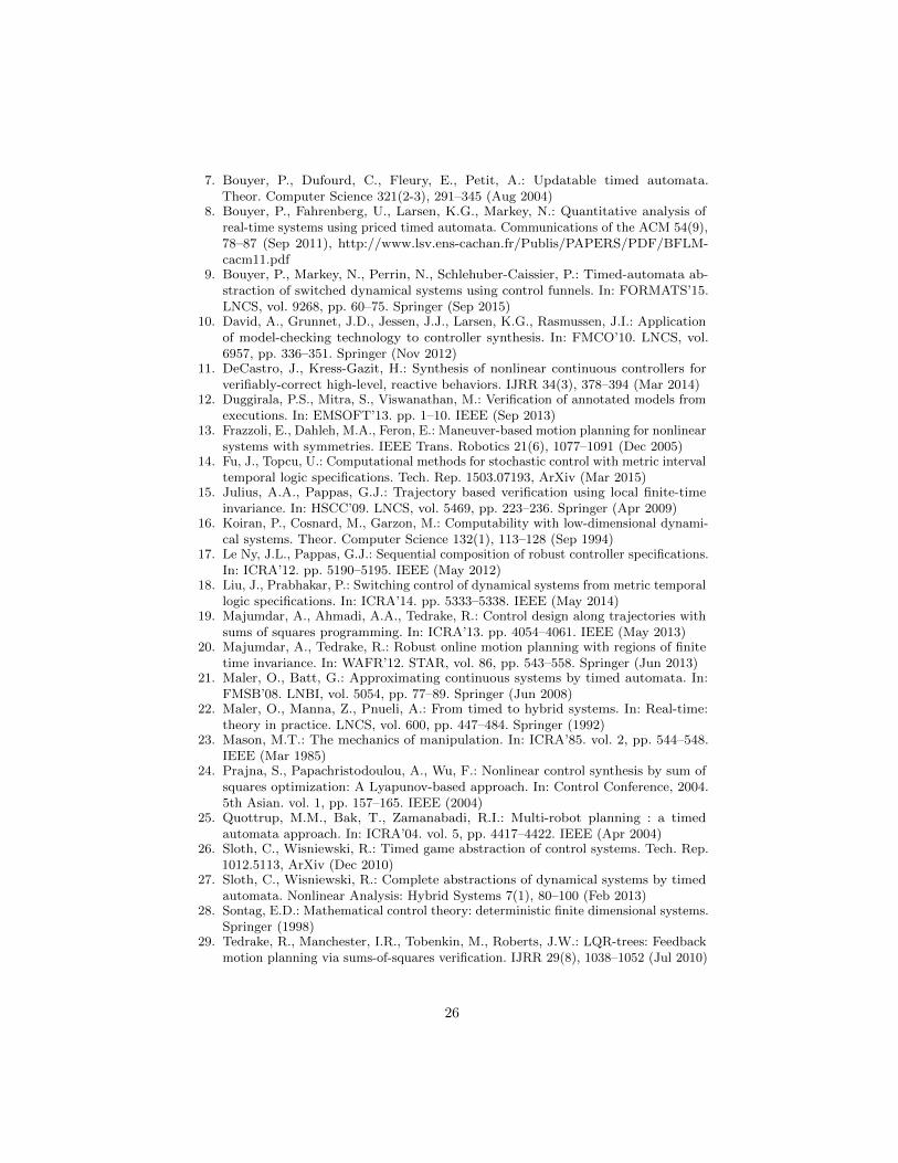
7. Bouyer, P., Dufourd, C., Fleury, E., Petit, A.: Updatable timed automata.Theor. Computer Science 321(2-3), 291–345 (Aug 2004)

8. Bouyer, P., Fahrenberg, U., Larsen, K.G., Markey, N.: Quantitative analysis ofreal-time systems using priced timed automata. Communications of the ACM 54(9),78–87 (Sep 2011), http://www.lsv.ens-cachan.fr/Publis/PAPERS/PDF/BFLM-cacm11.pdf

9. Bouyer, P., Markey, N., Perrin, N., Schlehuber-Caissier, P.: Timed-automata ab-straction of switched dynamical systems using control funnels. In: FORMATS’15.LNCS, vol. 9268, pp. 60–75. Springer (Sep 2015)

10. David, A., Grunnet, J.D., Jessen, J.J., Larsen, K.G., Rasmussen, J.I.: Applicationof model-checking technology to controller synthesis. In: FMCO’10. LNCS, vol.6957, pp. 336–351. Springer (Nov 2012)

11. DeCastro, J., Kress-Gazit, H.: Synthesis of nonlinear continuous controllers forverifiably-correct high-level, reactive behaviors. IJRR 34(3), 378–394 (Mar 2014)

12. Duggirala, P.S., Mitra, S., Viswanathan, M.: Verification of annotated models fromexecutions. In: EMSOFT’13. pp. 1–10. IEEE (Sep 2013)

13. Frazzoli, E., Dahleh, M.A., Feron, E.: Maneuver-based motion planning for nonlinearsystems with symmetries. IEEE Trans. Robotics 21(6), 1077–1091 (Dec 2005)

14. Fu, J., Topcu, U.: Computational methods for stochastic control with metric intervaltemporal logic specifications. Tech. Rep. 1503.07193, ArXiv (Mar 2015)

15. Julius, A.A., Pappas, G.J.: Trajectory based verification using local finite-timeinvariance. In: HSCC’09. LNCS, vol. 5469, pp. 223–236. Springer (Apr 2009)

16. Koiran, P., Cosnard, M., Garzon, M.: Computability with low-dimensional dynami-cal systems. Theor. Computer Science 132(1), 113–128 (Sep 1994)

17. Le Ny, J.L., Pappas, G.J.: Sequential composition of robust controller specifications.In: ICRA’12. pp. 5190–5195. IEEE (May 2012)

18. Liu, J., Prabhakar, P.: Switching control of dynamical systems from metric temporallogic specifications. In: ICRA’14. pp. 5333–5338. IEEE (May 2014)

19. Majumdar, A., Ahmadi, A.A., Tedrake, R.: Control design along trajectories withsums of squares programming. In: ICRA’13. pp. 4054–4061. IEEE (May 2013)

20. Majumdar, A., Tedrake, R.: Robust online motion planning with regions of finitetime invariance. In: WAFR’12. STAR, vol. 86, pp. 543–558. Springer (Jun 2013)

21. Maler, O., Batt, G.: Approximating continuous systems by timed automata. In:FMSB’08. LNBI, vol. 5054, pp. 77–89. Springer (Jun 2008)

22. Maler, O., Manna, Z., Pnueli, A.: From timed to hybrid systems. In: Real-time:theory in practice. LNCS, vol. 600, pp. 447–484. Springer (1992)

23. Mason, M.T.: The mechanics of manipulation. In: ICRA’85. vol. 2, pp. 544–548.IEEE (Mar 1985)

24. Prajna, S., Papachristodoulou, A., Wu, F.: Nonlinear control synthesis by sum ofsquares optimization: A Lyapunov-based approach. In: Control Conference, 2004.5th Asian. vol. 1, pp. 157–165. IEEE (2004)

25. Quottrup, M.M., Bak, T., Zamanabadi, R.I.: Multi-robot planning : a timedautomata approach. In: ICRA’04. vol. 5, pp. 4417–4422. IEEE (Apr 2004)

26. Sloth, C., Wisniewski, R.: Timed game abstraction of control systems. Tech. Rep.1012.5113, ArXiv (Dec 2010)

27. Sloth, C., Wisniewski, R.: Complete abstractions of dynamical systems by timedautomata. Nonlinear Analysis: Hybrid Systems 7(1), 80–100 (Feb 2013)

28. Sontag, E.D.: Mathematical control theory: deterministic finite dimensional systems.Springer (1998)

29. Tedrake, R., Manchester, I.R., Tobenkin, M., Roberts, J.W.: LQR-trees: Feedbackmotion planning via sums-of-squares verification. IJRR 29(8), 1038–1052 (Jul 2010)

26