Department of Information Engineering and Computer Science

Master’s Degree inComputer Science

Final Dissertation

Timed NuXmvFormal verification of synchronous timed transition systems

Supervisors StudentRoberto Sebastiani Enrico MagnagoAlessandro Cimatti

Alberto Griggio

Academic year 2017/2018

Acknowledgments

I would like to express my gratitude to the whole Embedded System unit in FBK and its headAlessandro Cimatti. He has given me the possibility to develop this master thesis and acquire a deeperknowledge on the subject of model checking with particular focus on real time systems.Other than my supervisor, Alberto Griggio, who advised and supported me during each step of thiswork, I would like to thank also the researchers Marco Roveri and Stefano Tonetta. The first for hiscontribution in the design of the newly implemented software modules and for lending me his deepknowledge of the code-base. The second one for the encoding of the interval semantic required by MTLand validation of the infinite traces representation, execution and completion.I thank all my colleagues and friends for their support and different points of view on the many issuesfaced during this thesis work. Finally a special thanks to my family in the persons of my mother Monica,my father Pierluigi and my brother Valerio.

Contents

Summary 5

I Ground work 7

1 Introduction 71.1 Formal verification of real-time systems . . . . . . . . . . . . . . . . . . . . . . . . . . 8

2 Background 92.1 Transition systems . . . . . . . . . . . . . . . . . . . . . . . . . . . . . . . . . . . . . . 92.2 Timed transition systems . . . . . . . . . . . . . . . . . . . . . . . . . . . . . . . . . . 9

2.2.1 Timed automata . . . . . . . . . . . . . . . . . . . . . . . . . . . . . . . . . . . 102.3 Propositional logic . . . . . . . . . . . . . . . . . . . . . . . . . . . . . . . . . . . . . . 10

2.3.1 Validity, satisfiability, unsatisfiability, equivalence and equi-satisfiability . . . . 112.3.2 Complexity . . . . . . . . . . . . . . . . . . . . . . . . . . . . . . . . . . . . . . 11

2.4 Temporal logics . . . . . . . . . . . . . . . . . . . . . . . . . . . . . . . . . . . . . . . . 122.4.1 LTL . . . . . . . . . . . . . . . . . . . . . . . . . . . . . . . . . . . . . . . . . . 122.4.2 MTL . . . . . . . . . . . . . . . . . . . . . . . . . . . . . . . . . . . . . . . . . . 13

2.5 Formal verification of properties . . . . . . . . . . . . . . . . . . . . . . . . . . . . . . . 142.5.1 LTL model checking . . . . . . . . . . . . . . . . . . . . . . . . . . . . . . . . . 142.5.2 Symbolic model checking . . . . . . . . . . . . . . . . . . . . . . . . . . . . . . 152.5.3 SAT/SMT based model checking . . . . . . . . . . . . . . . . . . . . . . . . . . 15

3 State of the Art 203.1 Timed automata decidability . . . . . . . . . . . . . . . . . . . . . . . . . . . . . . . . 203.2 Region automata . . . . . . . . . . . . . . . . . . . . . . . . . . . . . . . . . . . . . . . 203.3 Zones automata and DBM . . . . . . . . . . . . . . . . . . . . . . . . . . . . . . . . . . 21

4 nuXmv 234.1 Input language . . . . . . . . . . . . . . . . . . . . . . . . . . . . . . . . . . . . . . . . 23

4.1.1 Supported types . . . . . . . . . . . . . . . . . . . . . . . . . . . . . . . . . . . 234.1.2 Variables declarations . . . . . . . . . . . . . . . . . . . . . . . . . . . . . . . . 234.1.3 Define declarations . . . . . . . . . . . . . . . . . . . . . . . . . . . . . . . . . . 244.1.4 Constants declarations . . . . . . . . . . . . . . . . . . . . . . . . . . . . . . . . 244.1.5 Constraints . . . . . . . . . . . . . . . . . . . . . . . . . . . . . . . . . . . . . . 244.1.6 MODULE declarations . . . . . . . . . . . . . . . . . . . . . . . . . . . . . . . . 244.1.7 Specifications . . . . . . . . . . . . . . . . . . . . . . . . . . . . . . . . . . . . . 24

4.2 Model example . . . . . . . . . . . . . . . . . . . . . . . . . . . . . . . . . . . . . . . . 254.3 Trace simulation, execution and completion . . . . . . . . . . . . . . . . . . . . . . . . 26

4.3.1 Simulation . . . . . . . . . . . . . . . . . . . . . . . . . . . . . . . . . . . . . . . 264.3.2 Execution . . . . . . . . . . . . . . . . . . . . . . . . . . . . . . . . . . . . . . . 264.3.3 Completion . . . . . . . . . . . . . . . . . . . . . . . . . . . . . . . . . . . . . . 27

1

II Contribution 28

5 Input language extension 285.1 Definition of timed transition system . . . . . . . . . . . . . . . . . . . . . . . . . . . . 28

5.1.1 Time domain . . . . . . . . . . . . . . . . . . . . . . . . . . . . . . . . . . . . . 285.1.2 Clocks . . . . . . . . . . . . . . . . . . . . . . . . . . . . . . . . . . . . . . . . . 295.1.3 non-continuous variables . . . . . . . . . . . . . . . . . . . . . . . . . . . . . . . 295.1.4 Constraints . . . . . . . . . . . . . . . . . . . . . . . . . . . . . . . . . . . . . . 29

5.2 Specifications . . . . . . . . . . . . . . . . . . . . . . . . . . . . . . . . . . . . . . . . . 295.2.1 timed next, timed previous operators . . . . . . . . . . . . . . . . . . . . . . . . 305.2.2 at next, at last operators . . . . . . . . . . . . . . . . . . . . . . . . . . . . . . . 305.2.3 time since, time until operators . . . . . . . . . . . . . . . . . . . . . . . . . . . 30

5.3 Comparison with timed automata . . . . . . . . . . . . . . . . . . . . . . . . . . . . . . 31

6 Timed to Untimed system 326.1 variables . . . . . . . . . . . . . . . . . . . . . . . . . . . . . . . . . . . . . . . . . . . . 326.2 INIT . . . . . . . . . . . . . . . . . . . . . . . . . . . . . . . . . . . . . . . . . . . . . . 326.3 TRANS . . . . . . . . . . . . . . . . . . . . . . . . . . . . . . . . . . . . . . . . . . . . 326.4 INVAR . . . . . . . . . . . . . . . . . . . . . . . . . . . . . . . . . . . . . . . . . . . . 326.5 URGENT . . . . . . . . . . . . . . . . . . . . . . . . . . . . . . . . . . . . . . . . . . . 33

7 Timed properties verification 347.1 Property rewriting . . . . . . . . . . . . . . . . . . . . . . . . . . . . . . . . . . . . . . 34

7.1.1 next and previous operators . . . . . . . . . . . . . . . . . . . . . . . . . . . . . 347.1.2 until and since operators . . . . . . . . . . . . . . . . . . . . . . . . . . . . . . . 347.1.3 at next and at last . . . . . . . . . . . . . . . . . . . . . . . . . . . . . . . . . . 357.1.4 time since and time until . . . . . . . . . . . . . . . . . . . . . . . . . . . . . . 357.1.5 time and iota constraints . . . . . . . . . . . . . . . . . . . . . . . . . . . . . . 357.1.6 Diverging time . . . . . . . . . . . . . . . . . . . . . . . . . . . . . . . . . . . . 36

8 Timed traces 378.1 Representation . . . . . . . . . . . . . . . . . . . . . . . . . . . . . . . . . . . . . . . . 37

8.1.1 Discrete Infinite Trace . . . . . . . . . . . . . . . . . . . . . . . . . . . . . . . . 378.1.2 Timed trace . . . . . . . . . . . . . . . . . . . . . . . . . . . . . . . . . . . . . . 38

8.2 Simulation . . . . . . . . . . . . . . . . . . . . . . . . . . . . . . . . . . . . . . . . . . . 388.3 Execution . . . . . . . . . . . . . . . . . . . . . . . . . . . . . . . . . . . . . . . . . . . 388.4 Completion . . . . . . . . . . . . . . . . . . . . . . . . . . . . . . . . . . . . . . . . . . 398.5 From discrete to timed counter-example . . . . . . . . . . . . . . . . . . . . . . . . . . 40

9 Experimental evaluation 419.1 Description of the tools . . . . . . . . . . . . . . . . . . . . . . . . . . . . . . . . . . . 41

9.1.1 Uppaal . . . . . . . . . . . . . . . . . . . . . . . . . . . . . . . . . . . . . . . . . 419.1.2 ATMOC . . . . . . . . . . . . . . . . . . . . . . . . . . . . . . . . . . . . . . . . 429.1.3 LTSmin . . . . . . . . . . . . . . . . . . . . . . . . . . . . . . . . . . . . . . . . 439.1.4 Timed nuXmv . . . . . . . . . . . . . . . . . . . . . . . . . . . . . . . . . . . . 44

9.2 Benchmarks and results . . . . . . . . . . . . . . . . . . . . . . . . . . . . . . . . . . . 449.2.1 Fischer mutual exclusion algorithm . . . . . . . . . . . . . . . . . . . . . . . . . 449.2.2 Diesel generator . . . . . . . . . . . . . . . . . . . . . . . . . . . . . . . . . . . . 51

10 Conclusions 5410.1 Future work . . . . . . . . . . . . . . . . . . . . . . . . . . . . . . . . . . . . . . . . . . 54

10.1.1 Language constraints . . . . . . . . . . . . . . . . . . . . . . . . . . . . . . . . . 5410.1.2 Continuous variables . . . . . . . . . . . . . . . . . . . . . . . . . . . . . . . . . 5410.1.3 Timed CTL verification . . . . . . . . . . . . . . . . . . . . . . . . . . . . . . . 5410.1.4 Handle more complex infinite traces . . . . . . . . . . . . . . . . . . . . . . . . 55

2

10.1.5 Parameter synthesis . . . . . . . . . . . . . . . . . . . . . . . . . . . . . . . . . 55

Bibliography 55

3

4

SummaryContextThis thesis is placed in the context of formal verification of real-time systems. Most state-of-the-arttools require the real-time system to be modeled as a timed automaton. This is a well known andstudied formal representation that restricts the number of handled problem instances to a decidablefragment. The main techniques applied to solve these verification problems are described in chapter 3.This work presents an extension of the nuXmv symbolic model checker developed by the EmbeddedSystem unit in Fondazione Bruno Kessler. The tool previously supported the verification of discretefinite and infinite synchronous transition systems and it is now able to handle the verification of complextime properties on real-time systems.

MotivationsReal-time systems can be found in many technological devices and, in particular, in embedded systems.Often they are key components of safety-critical processes and devices. Some application domains are,for example, health-care, transportation and avionics. In recent years their complexity is steadilygrowing and the need for accurate and reliable systems able to ensure their quality has become evengreater. In many safety-critical domains model checking has been adopted. These techniques arecapable of fully verifying a system design against some properties. However, most state-of-the-arttechnologies available to perform this task on real-time systems suffer from limited scalability andexpressiveness with respect to properties. In particular not many of them allow to check specificationswith complex timing constraints which are fundamental for this kind of systems.

Contribution: formal verification of synchronous timed transitionsystems with dense time domainThe contribution of this thesis is the development of a new version, called Timed nuXmv, of the nuXmvmodel checker. The new software components are fully integrated in nuXmv and the new version iscompletely back-ward compatible. Timed nuXmv supports the same main functionalities supportedby nuXmv: model compilation, simulation, counter example generation, trace visualization, trace re-execution and trace completion. The following paragraphs give a high level description of how thesefeatures have been designed and implemented in Timed nuXmv.

Input language extension

The nuXmv input language has been extended with a model annotation, an additional type of variables(clock), a type modifier, a new constraint type (urgent) and four new operators are available in LinearTemporal Logic (LTL) specifications. These new constructs allow to describe timed transition systemswith continuous time semantic. The model description is parsed and compiled in the internal datastructures that have been extended to correctly represent the new elements. A more detailed descriptionof the input language of Timed nuXmv is provided in chapter 5.

Reduction to discrete infinite transition system

This work refers to time-unaware structures as discrete or untimed, while untiming is the process thatreduces a time-aware representation into an equivalent untimed one. Chapter 6 describes the untimingprocedure for Timed nuXmv models: their are reduced into an equivalent representation of a discreteinfinite transition system. Section 7.1 shows the untiming procedure applied to specifications. Theobtained untimed model with the associated specifications can be stored to file as a valid discreteSMV model. Therefore it is also possible to handle it using nuXmv without time extension. In TimednuXmv, to complete the reduction, the trace obtained on the discrete model is transformed into thecorresponding execution of the timed transition system that violates the specification. This procedureis described in section 8.5.

5

TracesnuXmv traces are able to represent only finite or lazo-shaped executions. They are not expressiveenough to represent traces of a timed transition system. In these executions the symbol representingtime does not follow these patterns: it is monotonically increasing. For this reason, in chapter 8, amore expressive trace representation, called infinite trace, is introduced. These traces allow to specifya subset of symbols whose value in loops is defined by a recurrence relation. These symbols, in thiswork, are called diverging. Timed nuXmv can show these infinite traces in all four formats that areavailable for nuXmv traces. They can also be loaded into the system from an external file.

Timed traces simulation

Timed nuXmv allows to simulate the execution of the input timed transition system. As nuXmv, itallows to choose between two possible modes: automatic and interactive. In the automatic mode anexecution of length up to a given constant it built. In the interactive mode at each step the system asksthe user to choose between a time elapse or a discrete transition, then the user is required to choosethe next state of the execution from a list of possible states. This functionality allows to inspect thepossible behaviors of a model. A detailed description is given in section 8.2.

Timed traces execution

It is also possible to check if a given execution is valid with respect to a model description. In the caseof infinite traces this implies that the loop has to be validated with respect to the diverging symbols.It is necessary to prove that the described system is allowed to repeat that loop infinitely many times,therefore that the loop of the infinite trace represents a valid infinite execution of the model. Thisproblem is encoded as a unsatisfiability problem of a SMT formula. The formula is such that it issatisfied by a model if and only if there exist an iteration number in which a transition of the loopviolates the conditions prescribed by the model. This formulation is shown and explained in section8.3.

Timed traces completion

Section 8.4 describes how the completion of partial infinite traces is performed in Timed nuXmv. Dueto the complexity class of the completion problem, in this version of Timed nuXmv, a more efficient,sound but incomplete procedure has been implemented. The system picks a possible completion andthen checks if the completed trace is a valid execution by exploiting the feature described above.

Experimental evaluationChapter 9 presents the experimental evaluation of Timed nuXmv. The software is compared to someother state-of-the-art tools on the verification of some invariant and MTL specifications on two differentkinds of models. In these benchmarks the newly implemented techniques showed good scalability interms of time and memory consumption with respect to the model size. In section 10.1 some possibledirections to further improve and extend the implemented procedures are highlighted. Particularattention is given to the constraints on the modeling and specification languages and to the kind ofinfinite behaviors that the system is able to detect and represent. For each direction some preliminaryobservations are reported.

6

Part I

Ground work

The first part of this thesis describes the theoretical background and existing tools upon which thiswork relies. Chapter 1 gives an introduction to the topic of formal verification of real-time systems andprovides some motivating examples. In chapter 2 the theoretical background required to understandthis work is introduced. First the structures used to represent a model are described, then the syntaxand semantic of the formal languages used to express specifications is defined, finally the last sectionof this chapter describes the main techniques used to perform the verification tasks. Chapter 3 brieflyreports the most relevant results on the decidability of some problems on models of real-time systems,then it describes the main verification procedures for such systems used by tools in the state of the art.Chapter 4 describes the relevant features that the symbolic model checker nuXmv supported beforethis thesis work. Particular attention is given to the input language (4.1) and to the operations ontraces (4.3). These chapters do not provide a complete description, but focus only on the aspectsthat are most relevant to this work. In particular some topics are only cited and some references areprovided for further readings.

The second and last part of this work (II) describes the actual contribution of this thesis. The addi-tional features of the modeling and specification languages are described, the reduction and verificationprocedures are explained, the supported operation on traces are shown and finally the implementedtechniques are compared with other state-of-the-art model checkers.

1. IntroductionIn engineering solving a problem often involves the design and construction of a system (hardware,software or both) to address specific tasks. An error in such systems might lead to undesirable effects.In some application domains, like space, avionics, transportation and health-care, these effects cancause heavy economic losses and physical injuries. For these reasons the definition of a developmentprocess that minimizes the probability of such events is critical. In the past there have been manyfailures of this kind, two of them are reported here as motivating examples. In 1993 a bug wasdiscovered in the Intel Pentium chip, floating point divisions in a certain range lead incorrect results.$475 million was the cost sustained by Intel to replace the defective chips [1]. Between 1982 and1985 the Therac25 radiation therapy machine was involved in at least six accidents. These machinescontained two software faults that, in some conditions, caused them to deliver a dose of beta radiationsapproximately 100 times the intended one [28].A common approach to address this issues is to perform extensive tests on a completely developedproduct. This technique has two major disadvantages: it requires a fully fledged system to be performedand, assuming the system to be deterministic, it only guarantees that it behaves correctly in thatparticular cases. In this approach mistakes made in the early stages will be detected only at the end ofthe development process. From these observations the need for tools that support the early phases ofthe development becomes evident. Over the years many formalisms to represent different points of view

7

of a system have been proposed and used in many application scenarios. These more or less formalrepresentations allow the designers to provide a model that is precise enough to highlight possibleinconsistencies and ease the review process. The modeling language should provide an abstraction asclose as possible to the application scenario in order to reduce the cost of creating such model anddecreases the probability of incurring modeling errors.For these reasons many companies and agencies, like Boeing, Airbus, ESA, NASA, Intel and RFI,integrated in their development process formal verification procedures. Moreover, also design tools likeSimulink provide formal verification features.

This thesis work is concerned with the modeling and verification of synchronous real-time systems.Real-time systems are becoming pervasive, often in the form of embedded devices; their applicationdomains range from transportation and automation in industries to economics and health-care. Overthe years their complexity has increased and people rely on them to perform critical tasks with absoluteprecision and reliability.

1.1. Formal verification of real-time systemsIn automated formal verification, given a description of the system and a property in some formallanguage, the machine is able to determine whether the system satisfies the property in all possibleexecutions; if it does not a counter-example is usually provided. There are many software products,called model checkers, that address this issue by exploiting different techniques to solve the verificationproblem and by providing different languages for describing the system and specify properties. Someexamples of such tools are: ATMOC, LTSmin, nuXmv and Uppaal.

The correctness of a real-time system depends not only on the logical result of the computationbut also on the time required to compute such result. Many safety-critical systems have hard real-time constraints; some examples are: defense and space systems, networked multimedia systems andembedded automative electronics. In this application scenario tools that allow to verify the systemdesign against its real-time requirements are fundamental to achieve a better quality and reliability ofthe final system. However, as highlighted in chapters 2 and 3, depending on the kind of constraints thisclass of verification problems quickly becomes undecidable. Most state-of-the-art techniques carefullylimit the expressiveness of their modeling languages to restrict the input models only to decidableinstances. These restrictions forbid the verification of systems with complex time behaviors that arenot expressible in such languages. It is still possible to provide a sound/correct answer in some ofthese cases, while due to the undecidability issue completeness is impossible to achieve. Increasing thenumber of behaviors for which the verification procedure is able to provide an answer, broadens theapplicability of these techniques to safety-critical domains with more complex dynamics.

This work describes how the nuXmv symbolic model checker has been extended to handle theverification of synchronous real-time systems. The new version of the tool is called Timed nuXmv.Both language and performance of the newly implemented software are compared to other relatedstate-of-the-art model checkers.

8

2. BackgroundThis chapter provides the definition of the terminology and key concepts that are used throughout thisthesis. An extensive presentation of most of the notions introduced in this chapter can be found inthe work of Baier and Katoen [5]. The chapter is organized as follows: first the formal structures usedto formally represent the systems are introduced. In particular different notations used to representtransition systems are defined. Among these, the notion of timed transition systems is central to thisthesis. Later both syntax and semantic of the most relevant formal languages used to specify propertieson these systems are explained. In the end the three main approaches used to verify such propertieson these models are presented.

2.1. Transition systemsThe formal description of the model is given as a transition system [5]. A transition system is adirected graph in which the nodes represent all possible states of the system and the edges representall possible transitions from a state to another. A subset of the nodes represents the initial states:all possible configuration from which the model can start. Every path on the graph starting from aninitial state represents a possible execution of the system and it is uniquely identified by a, possiblyinfinite, sequence of states. A state s is said to be reachable if there exist a path from an initial stateto s. States with no outgoing edges are called dead-lock states. From an automata-theoretic point ofview it is possible to borrow a slightly different terminology: the set of all possible executions of thetransition system is also called language of the automata and every execution is a word.

Two transition systems T, T ′ are said equivalent if they accept the same language:T ≡ T ′ ⇐⇒ L(T ) = L(T ′), where L is a function that given a transition system it computes itslanguage. The synchronous composition operator given two transition systems T0, T1 computes anothertransition system T such that its language L(T ) is the intersection of the languages of T0 and T1:T ..= T0 × T1 ⇐⇒ L(T ) = L(T0) ∩ L(T1). This operator is defined for each kind of transition systemand its usage is shown in the formal verification procedures.

Fair transition system A fair transition system is a transition system enriched with a set of oneor more fairness conditions. These additional constraints define a list of subsets of states. Every validexecution of the system infinitely often reaches at least one state in each one of these sets. The fair-ness conditions allow to impose progress constraints on the model executions which are not otherwiseexpressible in a transition system.

There are many different representations of transition systems, e.g. Kripke structures and Büchiautomata. They are slightly different notations to represent these objects, each of them can alsorepresent fairness conditions and has a synchronous product operator to compute the language inter-section. This work focuses on symbolic transition systems. These objects can be defined as a tripleM ..= (S, I, T ) where:

• S is a set of symbols, also called variables.• I is a propositional logic formula over the variables in S, this formula represents the set of initial

states.• T is a formula that defines the relation between the current and the next state, all transitions

that satisfy this formula are valid transitions.Sometimes they are defined using a 4-tuple M ..= (S, I,N, T ). This is an equivalent notation in whichN allows to explicitly state invariants of the transition system. The invariants can be represented inT as N ∧N ′, where N ′ refers to the next state assignments. Thus forbidding any transition startingfrom or leading to a state in which N is not satisfied.

2.2. Timed transition systemsIn discrete (or untimed) transition systems changes happen atomically and the evolution of the modelis given by a sequence of discrete steps. Timed transition systems extend discrete systems with the

9

notion of time: a new kind of variables is introduced. These variables, called clocks, keep track oftime elapses. A transition in a timed system is either a discrete step or a time elapse. During a timeelapse all discrete variables retain their values while all clock variables increase of the same amount,equal to the time elapsed.

Timed automataA timed automaton [4] is a transition system that can be represented by a finite graph in which nodesare called locations and edges represent discrete transitions. All clock variables are initialized to 0 andtime can elapse inside locations constrained by some location invariant. Every discrete transition isassociated with a guard condition and a set of clocks called reset. The automaton can perform atransition only if it satisfies the guards on such edge and when such transition is performed all clockvariables specified in its reset are set to 0.Location invariants impose progress conditions on the automaton, they forbid the system to stay inthe same location indefinitely, while guards and resets on the edges constrain its behavior.Given a set of clocks X, a clock variable x ∈ X and a rational constant c ∈ Q, let B(X) be the languagedefined by:

ϕ :: x ≤ c | c ≤ x | x < c | c < x | ϕ0 ∧ ϕ1 (2.1)

This language defines the set of clock constraints that can be expressed in a timed automaton. Noticethat it contains only conjunctions of comparisons with constants.Formally a timed automaton M is a 6-tuple M ..= (L,L0,Σ, X, I, E) where:

• L is a finite set of locations;• L0 ⊆ L is the set of initial location;• Σ is the set of labels;• X is the set of clock variables;• I : N → B(X) maps every location to its invariant condition;• E ⊆ L × B(X) × Σ × 2X × L is the set of edges, each edge has a starting location, a guard, a

label, a set of clock to be reset and a target location;The syntax l g,a,r−−−→ l′ is equivalent to (l, g, a, r, l′) ∈ E, where l, l′ ∈ L are locations, g ∈ B(X) is a

guard, a ∈ Σ is a label and r ∈ 2X is the set of clock reset by the transition.A clock interpretation µ is a function that to every clock associates a value in R, µ : X → R|X|.

The semantic of a timed automaton is a timed transition system in which states are pairs (l, µ), wherel ∈ L is a location and µ is a clock interpretation. The transitions are defined by the following rules:

• let d ∈ R+, then (l, µ)d−→ (l, µ + d) ⇐⇒ (µ |= I(l)) ∧ ((µ + d) |= I(l)); it is possible to perform

a time elapse of d in location l if the clock interpretation at the beginning and at the end of thetransition satisfies the location invariant of l.

• (l, µ)a−→ (l′, µ′) ⇐⇒ ∃(l, g, a, r, l′) ∈ E : (µ |= g) ∧ (µ′ = [r 7→ 0]µ) ∧ (µ′ |= I(l′)); it is possible to

perform a discrete transition labeled with a ∈ Σ from location l to location l′ if the current clockinterpretation µ satisfies the guard g of the transition and the clock interpretation updated bythe reset r (µ′ = [r 7→ 0]µ) satisfies the location invariant of the target state l′.

An action of a timed automaton M is a pair (t, a) where a ∈ Σ is the label of the transitiontaken by the automaton M after t ∈ R+ time units from the start of the system. A trace of a timedautomatonM is defined as a sequence of actions ξ ..= (t0, a0), (t1, a1), . . . such that ∀i ≥ 0 : ti ≤ ti+1. Arun or execution of a timed automaton M ..= (L,L0,Σ, X, I, E) over a trace ξ ..= (t0, a0), (t1, a1), . . .

is a sequence of transitions: (l0, µ0)d1−→ a1−→ (l1, µ1)

d2−→ a2−→ (l2, µ2) . . . where ∀i ≥ 1 : ti = ti−1 + di and(l0, µ0) ∈ L0. The language of the timed automaton M , written L(M), is the set of all traces ξ forwhich there exist a run of M over ξ

2.3. Propositional logicThis section gives the basic definitions of the most relevant terminology used in logic. These conceptsare then used to define temporal logics, which are the most commonly used formal notation to expressproperties on transition systems.

10

A boolean formula in propositional logic ϕ is either a constant (>, ⊥), a propositional atom or aboolean operator applied to boolean formulae.

ϕ ..= > | ⊥ | atom | ϕ0 ∧ ϕ1 | ϕ0 ∨ ϕ1 | ¬ϕ0 | ϕ0 → ϕ1

where >, ⊥ are the constants representing respectively true and false and atom is an atomicproposition: a symbol whose value is either > or ⊥. A literal is either a propositional atom orits negation. Let Atoms be a function that computes the set of atomic propositions occurring in aformula.

A total truth assignment µ over a formula ϕ is a function that to every atom in ϕ associates eithertrue or false.

µ : Atoms(ϕ)→ {>,⊥}

A partial truth assignment µ over a formula ϕ is a function that for every atom in a subset ofAtoms(ϕ) it associates either true or false.

µ : A→ {>,⊥}, A ⊆ Atoms(ϕ)

A total truth assignment µ satisfies a formula ϕ (µ |= ϕ) if and only if:• µ |= Ai ⇐⇒ µ(Ai) = > with Ai ∈ Atoms(ϕ);• µ |= ¬ϕ ⇐⇒ µ 6|= ϕ• µ |= ϕo ∧ ϕ1 ⇐⇒ (µ |= ϕ0) ∧ (µ |= ϕ1)• µ |= ϕo ∨ ϕ1 ⇐⇒ (µ |= ϕ0) ∨ (µ |= ϕ1)• µ |= ϕo → ϕ1 ⇐⇒ (µ |= ϕ0)→ (µ |= ϕ1)

A partial truth assignment satisfies a formula if all its total extensions satisfy that formula.

Validity, satisfiability, unsatisfiability, equivalence and equi-satisfiabilityA formula ϕ is said:

• valid if ∀µ : µ |= ϕ, every truth assignment satisfies the formula,• satisfiable if ∃µ : µ |= ϕ, there is at least one truth assignment that satisfies the formula,• unsatisfiable if ∀µ : µ 6|= ϕ, no truth assignment satisfies the formula.

From these definitions it follows that ϕ is valid if and only if ¬ϕ is unsatisfiable:∀µ0 : µ0 |= ϕ ⇐⇒ ∀µ1 : µ1 6|= ¬ϕ. Two formulae ϕ and φ are equivalent, written ϕ ≡ φ, if and onlyif ∀µ : (µ |= ϕ ⇐⇒ µ |= φ), while two formulae are equi-satisfiable if and only if∃µ0 : µ0 |= ϕ ⇐⇒ ∃µ1 : µ1 |= φ. Notice that if two fomulae are equivalent then they are alsoequi-satisfiable, but the converse does not hold.

Moreover, by induction on the structure of the formula, it can be shown that the following equiva-lence relationships hold for every propositional formulae ϕ0 and ϕ1:

ϕ0 ≡ ¬¬ϕ0

ϕ0 ∨ ϕ1 ≡ ¬(¬ϕ0 ∧ ¬ϕ1)

ϕ0 ∧ ϕ1 ≡ ¬(¬ϕ0 ∨ ¬ϕ1)

ϕ0 → ϕ1 ≡ ¬ϕ0 ∨ ϕ1

Complexity

Given a formula ϕ with N propositional atoms (|Atoms(ϕ)| = N) there are 2N distinct truth assign-ments. The problem of deciding whether a formula is satisfiable (is there an assignment among the 2N

that satisfies ϕ?) is a well known and studied NP-complete problem and it is usually referred to asthe SAT problem. Deciding validity and unsatisfiability of a formula are coNP-complete problemssince their language is the complementary of SAT. It is possible to check if a formula is valid bydeciding whether the negated is unsatisfiable, and a formula ϕ is unsatisfiable if and only if ϕ 6∈ SAT.

11

2.4. Temporal logicsThis section provides some background on temporal logics. They extend the syntax and semantic ofpropositional logic (2.3) with temporal operators. Many different temporal logics have been defined,some examples are: LTL[30], CTL[20], CTL*[21], MTL[26][29] and TCTL[12][13]. A survey ontemporal logics can be found in [12] and [13]. This section introduces the syntax and semantic of LTLin 2.4.1 and MTL in 2.4.2.

Temporal logic is any system of propositions qualified in terms of time, they can be categorizedin linear temporal logics and branching logics. Linear temporal logics, like LTL and MTL, considerevery execution as a single time line. Every state of a run has a single well defined successor andconsists of a path with no branches starting from an initial state. On the other hand branching logics,like CTL, CTL* and TCTL, consider multiple time lines at a time. At every step there are multiplenext states that represent all the possible choices. In this kind of logics each run consists in a directedgraph rooted at an initial state, where the children of a node represent all possible next states of thesystem.

LTLLinear Temporal Logic (LTL)[30] is a temporal logic that reasons on model executions as single timelines. It extends propositional logic with temporal operators that allow to predicate over previousand next states of these executions. In this work the version of LTL extended with past operators isconsidered.

Syntax

An atomic proposition is a LTL formula, a boolean operator applied to LTL formulae is a LTL formula,a temporal operator applied to LTL formulae is a LTL formula.

ϕ :: > | ⊥ | atom | ϕ0 ∧ ϕ1 | ϕ0 ∨ ϕ1 | ¬ϕ0 | ϕ0 → ϕ1 |Xϕ | Gϕ | Fϕ | ϕ0Uϕ1 | Y ϕ | Hϕ | Oϕ

where atom is an atomic propositional formula and >, ⊥ are the constants representing respectivelytrue and false. Notice that with respect to propositional logic (2.3) the only difference are the temporaloperators. X (next), G (globally), F (finally) and U (until) are the operators that predicate over futurestates, while Y (yesterday or previous), H (historically), O (once) and S (since) are the operators thatallow to predicate over past states.

Semantic

The semantic of propositional boolean operators remains unchanged, the semantic of temporal opera-tors is defined on a path π ..= s0, s1, . . . as follows:

• Xϕ holds at the current state si iff ϕ holds at the next step:

π, si |= Xϕ ⇐⇒ π, si+1 |= ϕ

• Gϕ holds at the current step si iff in all future states ϕ will always hold:

π, si |= Gϕ ⇐⇒ ∀j ≥ i : π, sj |= ϕ

• Fϕ holds in the current state si iff after finitely many steps the path reaches a state in which ϕholds:

π, si |= Fϕ ⇐⇒ ∃j ≥ i : π, sj |= ϕ

• ϕ0Uϕ1 holds in si iff at some point in the future ϕ1 holds and ϕ0 holds in all states from thecurrent step to that point in the future:

π, si |= ϕoUϕ1 ⇐⇒ ∃j ≥ i : π, sj |= ϕ1 ∧ ∀i ≤ k < j : π, sk |= ϕ0

12

• Y ϕ holds in the current state si iff there exist at least one previous state and at the step ϕ held:

π, si |= Y ϕ ⇐⇒ i > 0 ∧ π, si−1 |= ϕ

• Hϕ holds at state si iff in all previous steps ϕ held:

π, si |= Hϕ ⇐⇒ ∀j ≤ i : π, sj |= ϕ

• Oϕ is satisfied in the current state si iff there exists at least one state in the past in which ϕheld:

π, si |= Oϕ ⇐⇒ ∃j ≤ i : π, sj |= ϕ

• ϕ0Sϕ1 holds in si iff at some point in the past ϕ1 held and ϕ0 held in all states from that stepexcluded up to the current step:

π, si |= ϕoSϕ1 ⇐⇒ ∃j ≤ i : π, sj |= ϕ1 ∧ ∀j < k ≤ i : π, sk |= ϕ0

Notice that the following equivalence relationships between temporal operators hold:

¬Xϕ ≡ X¬ϕ¬Gϕ ≡ F¬ϕFϕ ≡ >Uϕ

similarly for past operators it can be shown that:

¬Y ϕ ≡ Y ¬ϕ¬Hϕ ≡ O¬ϕOϕ ≡ >Sϕ

A path π ..= s0, s1, . . . satisfies property ϕ if and only if the property holds in its initial state:π |= ϕ ⇐⇒ π, s0 |= ϕ. A transition system M satisfies a LTL property ϕ, written M |= ϕ if and onlyif ∀π ∈M , executions of the transition system, π |= ϕ.

MTLMetric Temporal Logic (MTL)[26][29] extends LTL (2.4.1) with bounded versions of time operators. InLTL it is possible to predicate about relative time relationships between events. Given two events, LTLallows to check whether one happens before, together or after the other. Its not possible to quantifythe amount of time elapsed between them. MTL adds this possibility: it allows to quantitativelypredicate about time by placing explicit bounds on time operators. MTL is defined on continuous timesemantic. Each execution becomes a dense sequence of configuration, therefore the semantic of theLTL operators X (next) and Y (yesterday) becomes ambiguous.

Syntax

An atomic proposition is a MTL formula, a boolean operator applied to MTL formulae is a MTLformula, a temporal operator applied to MTL formulae is a MTL formula.

ϕ :: > | ⊥ | atom | ϕ0 ∧ ϕ1 | ϕ0 ∨ ϕ1 | ¬ϕ0 | ϕ0 → ϕ1 |Gϕ | Fϕ | ϕ0Uϕ1 | Hϕ | Oϕ |ϕ0 UI ϕ1 | GIϕ | FIϕ | HIϕ | OIϕ

I :: [l, u] | (l, u] | [l, u) | (l, u) | [l,+∞) | (l,+∞)

where l and u are integer constants, +∞ represent positive infinite, atom is an atomic propositionalformula, >, ⊥ are the constants representing respectively true and false.

13

Notice that with respect to LTL (2.4.1) the only difference are the bounded temporal operators:UI , GI , FI , HI and OI and the absence of X and Y .

Semantic

The semantic of LTL and propositional operators is unchanged; the semantic of bounded temporaloperators is defined on a path π, where π(t) represents the total assignment over all symbols of themodel defined by such execution at time t ∈ R+.

For some time interval I, the bounded time operators are defined as follows:

• GIϕ holds at the current state π(t) iff ϕ holds in all configurations in the time interval I:

π(t) |= G[l, u]ϕ ⇐⇒ ∀k ∈ I : π(t+ k) |= ϕ

• FIϕ holds at the current state π(t) iff ϕ holds in a configuration in the time interval I:

π(t) |= FIϕ ⇐⇒ ∃k ∈ I : π(t+ k) |= ϕ

• ϕ0 UI ϕ1 holds at the current state π(t) iff ϕ1 holds at some point in the interval I and untilthat time ϕ0 holds:

π(t) |= ϕ0 UI ϕ1 ⇐⇒ ∃j ∈ I, j > 0 : π(t+ j) |= ϕ1 ∧ ∀t < k < j π : s(t+ k) |= ϕ0

• HIϕ holds at the current state π(t) iff ϕ held in all configurations between in I:

π(t) |= GIϕ ⇐⇒ ∀l ∈ I : π(t− k) |= ϕ

• OIϕ holds at the current state π(t) iff ϕ held in a configuration in interval I:

π(t) |= FIϕ ⇐⇒ ∃l ∈ I : π(t− k) |= ϕ

Notice that all time intervals are interpreted relatively to the time t of the current state.

2.5. Formal verification of propertiesThis section provides a brief introduction of the main techniques applied to solve the model checkingproblem: M |= ϕ. This thesis focuses on the verification of properties expressed in LTL and a fragmentof MTL. Three main approaches to model checking are shown: explicit state, symbolic and SAT/SMTbased. This work is mostly interested in the symbolic and SMT based techniques. The last approachis a category of techniques that involves procedures like: bounded model checking, K-induction andIC3.

Formal verification is concerned with proving or disproving the correctness of some system withrespect to certain specifications. A prominent approach to formal verification is model checking.Given a formal description of the system and a specification, usually expressed in logic, it performsan exhaustive exploration of the model in order to check whether the specification holds. When thespecification is violated these techniques are able to provide a representation of the model executionthat does not satisfy the property, this trace is called counter-example.

LTL model checkingThis section shows the main result used to perform LTL model checking, both in explicit state andsymbolic approaches. The verification problem is reduced to checking the language emptiness of atransition system.

Let M be a transition system and ϕ an LTL specification to be verified on M . The model checkingproblem M |= ϕ can be stated in terms of language inclusion as L(M) ⊆ L(ϕ). This implies thatL(M) ∩ L(ϕ) = ∅, where L(ϕ) is the set of all execution that do not satisfy ϕ (set complement).From the definition L(ϕ) = L(¬ϕ), substituting this in the previous formulation it is possible to

14

obtain L(M) ∩ L(¬ϕ) = ∅. Let M¬ϕ be a transition system such that L(M¬ϕ) = L(¬ϕ), thenL(M)∩L(M¬ϕ) = ∅. Since the language intersection of two transition system is equal to the languageof the automaton given by their synchronous composition: L(M ×M¬ϕ) = ∅.

In explicit state model checking these operations are performed on the graph that represents thetransition system, while in the symbolic technique SAT/SMT formulae that represent sets of statesare manipulated. This allows to avoid the creation of the explicit graph. The language emptiness inexplicit state techniques can be easily decided by performing a visit on the graph and searching for alooping path starting from an initial state and such that the loop involves at least one fair state. Insymbolic techniques the same condition can be checked by resorting to symbolic CTL model checking.

Many details have been omitted in this brief explanation, in [5] it is possible to find a completedescription of both explicit state and symbolic LTL model checking. The following section provides amore detailed description of the symbolic approach; it also highlights the main differences with respectto explicit state techniques.

Symbolic model checkingThe explicit state techniques require to explicitly create and store the transition system. The numberof configurations may be exponentially large in the number of propositional atoms of the model. Inthese cases this kind of techniques quickly become too expensive to be performed. Symbolic modelchecking [5] tries to avoid this issue by manipulating sets of states at a time. This is achieved byrepresenting them as formulae in propositional logic. In a similar way, these techniques are able tomanipulate sets of transitions represented by propositional formulae expressed in terms of current andnext state variables. It is important to notice that all logically equivalent formulae represent the sameset of states or transitions. This allows to perform all the simplifications available in propositionallogic to obtain a more compact expression. This also implies that the size of a formula is not directlyrelated to the cardinality of the set it represents.

More formally, each state of the transition system is represented by an array of boolean statevariables V ..= (x0, x1, . . . , xk). Let ξ(s) be the symbolic representation of the state s, which is a totalassignment over V . A subset of states Q ⊆ S is represented by

∨s∈Q

ξ(s) and all equivalent formulae.

Set operations are mapped by boolean operators, in particular for P,Q ⊆ S:

ξ(P ∩Q) = ξ(P ) ∧ ξ(Q)

ξ(P ∪Q) = ξ(P ) ∨ ξ(Q)

ξ(S \ P ) = ¬ξ(P )

Transitions in R ⊆ (S × S) are represented by propositional formulae over V and V ′, where V ′

is the array of boolean variables representing their values after the transition. R can be symbolicallyrepresented by all formulae equivalent to:∨

(s,s′)∈R

ξ(s, s′) ≡∨

(s,s′)∈R

ξ(s) ∧ ξ(s′)

where ξ(s) is a total assignment over V and ξ(s′) is a total assignment over V ′.

SAT/SMT based model checkingSAT/SMT based techniques are symbolic techniques that reduce the verification problem to a sat-isfiability problem. They try to exploit the advancements in SAT and SMT fields to achieve betterscalability.

The SAT problem has already been introduced in section 2.3.2. Satisfiability Modulo Theory(SMT) is the problem of deciding whether a boolean formula has at least one model with respect tocombinations of background theories (e.g. reals, uninterpreted functions, arrays and bit vectors). Inan SMT instance predicates consist of boolean expressions on some underlying theories: x − 3 < 3.5is a SMT predicate over the reals. Some examples of SMT solvers are CVC4, MathSAT, SMT-RAT,Yices and Z3.

15

Bounded model checking

In bounded model checking [10] the execution of a model M is unrolled up to k steps. A single formularepresenting all executions of length k violating the specification ϕ is built. The formal verificationtask is solved by checking if there exists a model for such formula. The assignments prescribed bythis model represent a run of length k of M that violates the specification: a counter-example. Thisprocedure is iterated for increasing values of k until a counter-example is found. BMC is only capableof falsifying properties: if a property holds this procedure will never halt. For this reason it is oftenused in combination with K-induction (2.5.3).

LetM ..= (S, I, T ) be a transition system and ϕ be a LTL formula. Let [[ϕ]]ft be the BMC expansionof ϕ from step f ∈ N to step t ∈ N without loop-backs and l[[ϕ]]ft the encoding with loop-back from tto l. This encoding is straightforward for standard boolean operators, while more attention is requiredfor temporal operators.

ϕ [[ϕ]]ft l[[ϕ]]ftp p p

¬p ¬p ¬pϕ0 ∧ ϕ1 [[ϕ0]]

ft ∧ [[ϕ1]]

ft l[[ϕ0]]

ft ∧ l[[ϕ1]]

ft

ϕ0 ∨ ϕ1 [[ϕ0]]ft ∨ [[ϕ1]]

ft l[[ϕ0]]

ft ∨ l[[ϕ1]]

ft

Xϕ0if i ≥ k : ⊥,else : [[ϕ0]]

f+1t

if i ≥ k : l[[ϕ0]]lt,

else : l[[ϕ0]]f+1t

Gϕ0 ⊥t∧

j=min(l,f)l[[ϕ0]]

jt

Fϕ0

t∨j=f

[[ϕ0]]jt

t∨j=min(l,f)

l[[ϕ0]]jt

Table 2.1: BMC encoding

Xϕ corresponds to evaluating ϕ in the next state, if such state does not exists its false. Gϕ is trueonly if there is a loop and in each state of the loop ϕ holds. Fϕ holds if there exists a state from thebeginning to the k-th that satisfies ϕ. The until temporal operators has been omitted for brevity.

The BMC procedure at every step k checks if the propositional formula

I(s0) ∧n−1∧i=0

(T (si, si+1 ∧ ϕ(si)) ∧ ¬ϕ(sn)

is satisfiable. If a model for such formula exists, then its assignments are a counter-example for propertyϕ and it is possible to conclude that the specification is violated. Notice that the encoding generates asymbolic representation of all paths of length k starting from the initial states such that at every stepbut the last one ϕ holds. As already stated, the satisfiability check is performed by calling SAT orSMT procedures. The BMC technique performs one SAT/SMT call for every k. Subsequent encodingsshare most of the clauses, this can be exploited to improve scalability and decrease the running time.

K-induction

K-induction [31] complements BMC in the sense that it is able to verify properties. This techniquesymbolically identifies all states that violate an invariant property (bad states) and tries to prove thatnone of them is reachable. In order to do this it tries to show that there exist no path of length k thatends in a bad state. As in the BMC case this is repeated for increasing values of k. The paths arecreated by going backward from the bad states, if at step k no such path exists then the specificationholds, otherwise the procedure is repeated for k + 1. Notice that checking whether one of the pathsstarts from an initial state leads exactly to the BMC formulation.

16

As for the BMC case, let M ..= (S, I, T ) be a transition system and ϕ be a LTL formula. In theK-induction encoding there are two main components: one rules out all loops∧

0≤i<j≤k¬(si = sj)

and the other one builds a symbolical representation of paths of length k ending in a bad state

k∧i=0

(T (si, si+1) ∧ ϕ(si)) ∧ ¬ϕ(sk+1).

As in the BMC case subsequent encodings share most of the formula, moreover the formula thatcreates a path of length k is shared between BMC and K-induction. For this reason these two techniquesare often applied together exploiting the sharing and incrementality of these formulae to improveperformance.

IC3

Incremental Construction of Inductive Clauses for Indubitable Correctness (IC3) is a model checkingalgorithm invented by Aaron Bradley in 2010. In its original form it was meant to solve reachabilityproblems expressed in SAT. Later works extended it to deal also with liveness, incremental reasoningand SMT formulae. Experimentally IC3 appears to be superior to any other single solver used inthe hardware model checking competition [2]. This work first provides a high level description of thealgorithm in the propositional finite state case, as described by Aaron R. Bradley in [14], then tworelevant extensions to SMT infinite state are presented.

Propositional finite stateLet S be a transition system described by I(X), T (Y,X,X ′) that represent respectively the set ofinitial states and the transition relation; X and X ′ represent current and next state variables, while Yrepresents primary input variables to the system. Let P (X) describe a set of good states. The objectiveof the IC3 algorithm is to prove that all states reachable by S are good. This is achieved by findingan inductive invariant F (X) which proves that S satisfies P [17]. F (X) must be such that:

(a) I(X) |= F (X), the initial states satisfy the invariant;

(b) F (X) ∧ T (Y,X,X ′) |= F (X ′), every state reached in one step from a state that satisfies theinvariant also satisfies it;

(c) F (X) |= P (X), from the invariant its possible to conclude P .

Its easy to notice that the conjunction of these 3 requirements on F is sufficient to conclude that Pholds in every reachable configuration.

F is built by keeping a sequence, called trace, of formulae, called frames, F0(X), F1(X), . . . , Fk(X)such that:

• F0 = I, the first formula of the trace represents the initial states of the transition system;• ∀i > 0 Fi is a set of clauses: conjunction of disjunctions;• ∀0 < i < k : Fi+1 ⊆ Fi, which implies Fi |= Fi+1;• ∀0 < i < k : Fi(X)∧T (Y,X,X ′) |= Fi+1(X

′), the symbolic representation obtained by performinga single step from a given frame is a model for the following frame;

• ∀0 ≤ i < k : Fi |= P .Each Fi symbolically represents a superset, or over-approximation, of the set of states that the

machine M can reach in i steps. Therefore the trace F0(X), F1(X), . . . , Fk(X) represents an over-approximation of all possible executions of length k.

The IC3 procedure can be split into two main phases: a blocking and a propagation phase. Duringthe blocking phase the approximation is refined by adding additional clauses. If during this operationsome frame Fi becomes such that Fi ∧ ¬P 6|= ⊥: it has a non empty intersection between the states

17

it represents and the bad states, then its possible to reconstruct a counter-example using the framesF0, . . . , Fi. The propagation phase tries to extend the trace with an additional frame Fk+1. Thisframe is generated by moving forward the clauses of the previous Fi. If during this process for somei Fi = Fi+1 holds, then a fix point has been reached and Fi is the inductive invariant that proves theproperty.

The following section gives a more detailed description on how the approximation is refined. IC3maintains a set of proof obligations, which are pairs (s, i) such that i is the step index and s is acounter-example to induction (CTI). A CTI is symbolic representation of a set of states that mightnot be reachable from the initial states and have at least one successor that either is or can reach abad state. The unreachability of s from Fi−1 is recursively proved by checking whether ¬s is relativeinductive to Fi−1: Fi−1 ∧ ¬s ∧ T |= ¬s′. This can be decided by the unsatisfiability of:

Fi−1 ∧ ¬s ∧ T ∧ s′ (2.2)

If 2.2 is unsatisfiable and s does not contain any initial state, then ¬s can be used to strengthen Fi. Inparticular ¬s is generalized into a formula g which is added to Fi. This generalized formula g must besuch that g |= ¬s and it is relative inductive to Fi−1: it also makes 2.2 unsatisfiable. Since the objectiveof this section is to provide a high level intuition on how IC3 works, the description of the generalizationprocedure is omitted. If 2.2 is satisfiable, then either s is reachable or the over-approximation Fi−1 istoo coarse grained to prove its unreachability. Let c be the symbolic representation of the set of statessuch that (Fi−1 ∧ ¬s |= c) ∧ (∃Y : c(X) ∧ T (Y,X,X ′) |= s(X ′)). The states in c are a subset of theintersection of Fi−1 and ¬s, this intersection can not be empty since 2.2 is satisfiable by hypothesis.Moreover each state in c can reach a state in s′ in one step for some assignment over the input variablesY : they are in the preimage of s. To decide whether ¬s is reachable or not it is sufficient to check ifc is reachable from Fi−2. This corresponds to trying to block the proof obligation (p, i − 1). This isrepeated recursively until either the unreachability is proved or the first frame (i = 0) is reached. Inthe latter case the generated sequence of proof obligation represents a counter example for the propertyP on S.

SMT infinite state generalizationIC3 has been generalized to be applicable to SMT problems and infinite state transition systems.While in the previous case the problem was decidable, in this case it is not, therefore completeness isimpossible to achieve.In the SMT case if formula 2.2 is satisfiable a total assignment c in the preimage of s is obtained.Depending on the theory used, cmight represent a single point in an infinite space and as a consequencelead to a high chance of divergence in the blocking phase. For this reason it is necessary to generalizec into a set of predecessors of s.

In the literature it is possible to find different techniques to solve this problem: some rely onquantifier elimination [17], others try to obtain better performance by embedding in the generalizationprocedure theory specific procedures [22] and finally implicit abstraction techniques are less dependenton the specific underlying theory [19]. The following paragraphs provide a high level overview of theIC3 SMT generalization of the last two approaches.

Theory dependent generalization Hoder and Bjørner [22] in 2012 proposed an extension ofIC3 to the SMT case by embedding in the generalization of the CTI a theory dependent component.The propositional and theory specific procedures are combined together with the objective of obtaininga SMT formula g such that g |= ¬s and Fi−1 ∧ g ∧ T ∧ ¬g′ is satisfiable (2.2). In the case of linearrational arithmetic (LRA) after the boolean generalization procedure the algorithm tries to weakeninequalities of the form t ≤ c to t ≤ c+ c′ with c′ > 0 such that the SMT formula 2.2 still holds [22].

The main drawback of this approach is the requirement of a specialized generalization procedurefor each theory.

Implicit abstraction Cimatti et alii [19] in 2016 proposed IC3-IA: an abstraction based ex-tension to the infinite state SMT case of IC3 that does not require theory specific generalization

18

procedures. S is an abstraction of the transition system S if and only if every state reachable in S hasa corresponding abstract state reachable in S. This procedure allows to reduce the size of the statespace and improve the performance of the verification procedures. The abstract state space is inducedby a set of predicates P and generated by the abstraction relation HP(X,XP) ..=

∧p∈P

xp ↔ p(X), where

xp is a boolean variable of the abstract space. The predicate abstraction of a formula ϕ with respectto P, written ϕP is computed as:

ϕP(XP) ..= ∃X,X ′ : ϕ(X), X ′ ∧HP(X,XP)

ϕP(XP, X′P) ..= ∃X,X ′ : ϕ(X,X ′) ∧HP(X,XP) ∧HP(X ′, X ′P)

(2.3)

The IC3 procedure is modified to learn clauses over predicates in the abstract space. The predicateabstraction (2.3) is used to obtain an abstract transition relation T (X,Y ′) from T (X,X ′). This relationis replaced in 2.2 leading to:

F (X) ∧ s(X) ∧ T (X,Y ′) ∧ ¬s(X ′) ∧∧p∈P

(p(X ′)↔ p(Y ′)) (2.4)

s(X) is relative inductive to F (X) if formula 2.4 is unsatisfiable. If s(X) is relative inductive theinductive strengthening procedure described for the boolean case is applied, otherwise the abstractpredecessor c can be computed from the satisfying SMT model µ as:

c ..= {p(X) | p ∈ P ∧ µ |= p(X)} ∪ {¬p(X) | µ 6|= p(X)}

Notice that it is not necessary to compute the abstract transition relation T (X,Y ′) explicitly. Itcan be done implicitly by adding the abstraction procedure to the SMT formulation.

If property P holds in the abstract transition system S, then the original property P holds in theoriginal transition system S. Otherwise an abstract counter-example π ..= s0, s1, . . . , sk is generated.This execution of S might not correspond to any execution on S, it might be spurious. This canbe verified by considering the SMT formula representing all paths of the same length of π on theoriginal model and imposing the abstraction of each step to be the abstract state prescribed by π. Ifthis formula is unsatisfiable then π is spurious, otherwise the satisfying model provides an executionπ ..= s0, . . . , sk such that every si ∈ π is the abstract representation of si ∈ π and π 6|= P . If a spuriouscounter-example is identified, the set of predicates P is updated so that at least π is removed from thelanguage of S. In the literature many possible implementations of this refinement procedure have beendeveloped. However in this work they are not discussed, a more detailed explanation of this topic canbe found in [19].

It is relevant to notice that the selection of the predicates to be considered in P greatly affects theoverall performance.

19

3. State of the ArtAfter some general considerations about the decidability of some problem on timed automata, thischapter provides a description of the main state-of-the-art approaches in the field of formal verificationof timed transition systems. Tools implementing these techniques are used in chapter 9 to evaluatethe performance of Timed nuXmv for invariant and MTL checking.

3.1. Timed automata decidability

Alur and Dill in [3] and [4] show some interesting results about the complexity of some problemson timed automata. The reachability problem and checking language emptiness of timed automataare decidable, as in the discrete case, and they belong to the PSPACE-complete class. However, inthe same publications, they show that given two timed automata M and M ′, the language inclusionproblem L(M) ⊆ L(M ′) is undecidable. Moreover, as shown in [15], it is enough to allow additiveclock constraints to the timed automata language B(X) (2.1) to make also the emptiness checkingundecidable.

3.2. Region automata

Timed automata have real valued clocks, this implies that the state space of their transition systemis infinite. Most state-of-the-art approaches build a finite state abstraction of a timed automata. Thetime behavior of the system is represented by a finite set of equivalence classes called regions. Thissection describes the main procedure used to create this finite state abstraction of the infinite timedtransition system [5].The infinite state space is split into finitely many partitions by considering each of these partitionsas an abstract state. This allows to build a finite abstract state space. Every partition representsan equivalence class over the states of the timed transition system, these states are such that theyall exhibit the same behavior in the abstract space. Notice that, from the definition of B(X) (2.1),clocks are compared only with constants and, since the model description is finite, then for each clockx there are finitely many of such values in Q. Let cx be the maximum constant to which the clockx is compared to. Given two clock interpretations µ, µ′ : X → R|X|, let bµ(x)c be the integral partof the value associated to clock x by the interpretation µ, and let frac(µ(x)) ..= µ(x)− bµ(x)c be itsfractional part. This notation allows to define the equivalence relationship over clock interpretations.µ is equivalent to µ′, written µ ≡ µ′, if and only if the following conditions hold:

1. ∀x ∈ X : bµ(x)c = bµ′(x)c∨ (µ(x) > cx∧µ′(x) > cx), for every clock the interpretations µ and µ′

either agree on the integral part or the assigned values are greater than the maximum constantcorresponding to that clock variable.

2. ∀x, y ∈ X µ(x) ≤ cx ∧ µ(y) ≤ cy : frac(µ(x)) ≤ frac(µ(y)) ⇐⇒ frac(µ′(x)) ≤ frac(µ′(y)), forall pairs of clocks that are mapped to values smaller than their respective maximum constants,the two interpretations have the same ordering of the clocks based on their fractional part. Noticethat from the previous condition these two clocks share the same integral part.

3. ∀x ∈ Xµ(x) ≤ cx : frac(µ(x)) = 0 ⇐⇒ frac(µ′(x)) = 0, one interpretation assigns a valuewith fractional part 0 (an integer) smaller than the maximum constant associated to a clock ifand only if also the other interpretation assign an integer value to the same clock. Notice that,together with the first condition, this implies that they assign the same value.

These three conditions partition the infinite clock space R|X| into finitely many equivalence classescalled regions. Their number is finite since in each model there can be only a finite number of constants.

20

x

y

0 1 2 3 40

1

2

3

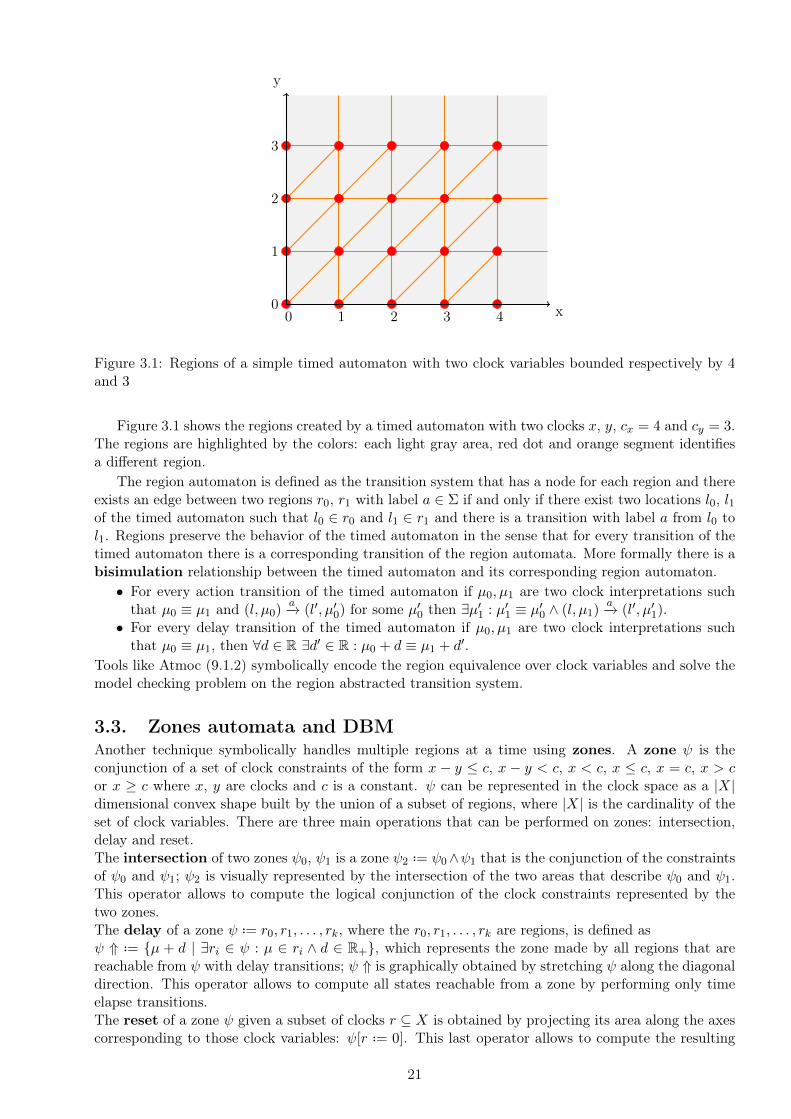
Figure 3.1: Regions of a simple timed automaton with two clock variables bounded respectively by 4and 3

Figure 3.1 shows the regions created by a timed automaton with two clocks x, y, cx = 4 and cy = 3.The regions are highlighted by the colors: each light gray area, red dot and orange segment identifiesa different region.

The region automaton is defined as the transition system that has a node for each region and thereexists an edge between two regions r0, r1 with label a ∈ Σ if and only if there exist two locations l0, l1of the timed automaton such that l0 ∈ r0 and l1 ∈ r1 and there is a transition with label a from l0 tol1. Regions preserve the behavior of the timed automaton in the sense that for every transition of thetimed automaton there is a corresponding transition of the region automata. More formally there is abisimulation relationship between the timed automaton and its corresponding region automaton.

• For every action transition of the timed automaton if µ0, µ1 are two clock interpretations suchthat µ0 ≡ µ1 and (l, µ0)

a−→ (l′, µ′0) for some µ′0 then ∃µ′1 : µ′1 ≡ µ′0 ∧ (l, µ1)a−→ (l′, µ′1).

• For every delay transition of the timed automaton if µ0, µ1 are two clock interpretations suchthat µ0 ≡ µ1, then ∀d ∈ R ∃d′ ∈ R : µ0 + d ≡ µ1 + d′.

Tools like Atmoc (9.1.2) symbolically encode the region equivalence over clock variables and solve themodel checking problem on the region abstracted transition system.

3.3. Zones automata and DBMAnother technique symbolically handles multiple regions at a time using zones. A zone ψ is theconjunction of a set of clock constraints of the form x − y ≤ c, x − y < c, x < c, x ≤ c, x = c, x > cor x ≥ c where x, y are clocks and c is a constant. ψ can be represented in the clock space as a |X|dimensional convex shape built by the union of a subset of regions, where |X| is the cardinality of theset of clock variables. There are three main operations that can be performed on zones: intersection,delay and reset.The intersection of two zones ψ0, ψ1 is a zone ψ2

..= ψ0∧ψ1 that is the conjunction of the constraintsof ψ0 and ψ1; ψ2 is visually represented by the intersection of the two areas that describe ψ0 and ψ1.This operator allows to compute the logical conjunction of the clock constraints represented by thetwo zones.The delay of a zone ψ ..= r0, r1, . . . , rk, where the r0, r1, . . . , rk are regions, is defined asψ ⇑ ..= {µ + d | ∃ri ∈ ψ : µ ∈ ri ∧ d ∈ R+}, which represents the zone made by all regions that arereachable from ψ with delay transitions; ψ ⇑ is graphically obtained by stretching ψ along the diagonaldirection. This operator allows to compute all states reachable from a zone by performing only timeelapse transitions.The reset of a zone ψ given a subset of clocks r ⊆ X is obtained by projecting its area along the axescorresponding to those clock variables: ψ[r ..= 0]. This last operator allows to compute the resulting

21

zone after the resets of a transition.The zone automaton is defined as a transition system in which states are pairs (l, ψ), where l is

a location and ψ a zone. Its transition relation is defined by:• (l, ψ) (l, ψ ⇑ ∧I(l)), where I(l) is the location invariant of l;• (l, ψ) (l′, ψ[r ..= 0] ∧ g ∧ I(l′)) if l g,a,r−−−→ l′

This definition of the zone automaton, corresponding to a timed automaton with initial state(l0, µ0), guarantees that:

• soundness: ((l0, µ0) ∗ (lf , ψf ))=⇒∃µf ∈ ψf : (l0, µ0)→∗ (lf , µf ), if a configuration is reachablein the zone automaton then there exists a corresponding reachable state in the timed automaton.

• completeness: (l0, µ0) →∗ (lf , µf )=⇒∃ψf : µf ∈ ψf ∧ ((l0, µ0) ∗ (lf , ψf )), if a configurationis reachable in the timed automaton then the corresponding zone is also reachable in the zoneautomaton.

Zones can be stored using Difference Bound Matrices (DBM). They efficiently support zones operationsand have a canonical representation. Let X0

..= X ∪ 0, where 0 is a reference clock. Every clockconstraint in a zone ψ is rewritten in the form x − y ◦ n where x, y ∈ X0 ∧ ◦ ∈ {<,≤}. ψ can berepresented in a |X0| × |X0| matrix M(ψ), where the first row and first column represent the referenceclock 0 and the others represent the other clocks in some order. Each cell of the matrix keeps trackof whether the bound is strict or not and the value of the bound itself: M(ψ)ij = (n, ◦) implies thatci − cj ◦ n for some ◦ ∈ {<,≤}.

Tools like Uppaal (9.1.1) and Opaal (9.1.3) use this kind of representation to handle to behaviorover time of the model, while the discrete development is handled using explicit state techniques. Thisimplies that the zone representation is done for each possible discrete location. For this reason thesekind of techniques usually scale well with respect to increasing time constraints. However, they areunable to manage complex discrete behavior since the number of states increases exponentially andthe explicit state representation of such systems becomes very large.

22

4. nuXmvThis work is grounded on the nuXmv model checker. nuXmv is actively maintained and used by theEmbedded System unit in Fondazione Bruno Kessler. It lies at the core of a set of other tools likeHyComp, Ocra and xSAP. It allows to analyze synchronous finite and infinite state systems. In thischapter the relevant fragment of the input language of nuXmv will be described along with its mainfunctionalities. In particular the model simulation and trace re-execution features will be presented.For a complete description please refer to the nuXmv user manual, [16] and [9].

4.1. Input languageIn this section the main constructs of the nuXmv input language will be described. For compactnessreasons this description will focus on the subset of most relevant features that are required for a betterunderstanding of the extensions and reduction technique presented in chapters 5, 6 and 7.

Supported typesBoolean Like most formal languages, nuXmv supports the boolean type which comprises thesymbolic values TRUE and FALSE.

Enumeration Enumeration types are sets of values, in particular three different types of enumera-tions are supported:

• symbolic enumeration: the elements of the set are all symbolic constants,e.g. {a, z, e, k, ya};

• integer enumeration: the elements of the set are all integer constants,e.g. {2, 6, 20, 17, -3};

• integer and symbolic enumeration: the elements of the set are either integer constants orsymbolic constants,e.g. {2, h, 20, k, -3}.

Word unsigned word[N] and signed word[N] are used to represent bit vectors of fixed lengthN. Signed vectors allow signed operations while unsigned vector allow unsigned operations. Signedwords are represented using the usual two’s complement.

Integer The domain of a variable of type integer is the whole set of integer numbers: Z. Thereforeis has an infinite discrete domain. However, in the input model it is possible to specify integer constantsonly in the range: [−232 + 1; 232 − 1].

Real The domain of a variable of type real is the whole set of rational numbers: Q. A rationalconstant can be expressed in the input model using the following syntax: f’3/4

Array Array types allow to model sequences of elements of other types. In particular it is possibleto specify the lower and upper bound for the index of the array and the type the elements in it. Theelement type can be an array type itself.

Variables declarationsVariables define the set of possible states of the model. A total assignment over the variables of amodel uniquely identifies a configuration of the system. The set of all possible configurations is thestate space. Every variable is associated to one of the types described above.

State variables State variables keep the system’s configurations, their values might change as thesystem evolves through transitions.

Input variables Input variables allow to model external inputs that are not under the control ofthe system. In particular these kind of variables allow to put labels on the transitions.

23

Frozen variables Frozen variables are variables that retain the same value for the whole modelexecution. Their initial value can be constrained in the same way of state variables. The reader maythink of fronzen variables as constant or immutable variables of other languages.

Define declarationsDefines allow to create symbols that are equivalent to another expressions. They are macros, sincewhenever a define identifier is found, it is syntactically replaced by the expression it is associated with.

Constants declarationsIn the nuXmv language it is possible to declare a set of symbolic constant that can be used in themodel description.

ConstraintsIn the following the main syntactical elements to describe a system behavior are presented.

INIT constraints INIT allows to specify the possible initial configurations of the system. Thisconstruct allows to specify symbolically the set of initial states: every state such that all the INITconstraints evaluate to TRUE is an initial state.

INVAR constraints INVAR allows to specify conditions that must be satisfied by every state of thesystem. Every INVAR constraints identifies a subset of valid states in the state space. The intersectionof all these sets is the set of valid states of the model.

TRANS constraints TRANS constraints allow to specify how the system evolves at each step. Thelanguage allows to access the value of a symbol x after the next transition using next(x). TRANSconstraints are predicates over current and next variables. The possible transitions of the systems areall pairs of current and next state that satisfy such predicates. If at a given state there are multipletransitions the system can choose any of them. Otherwise, if at a given state there are no validtransitions, such state is called deadlock state.

MODULE declarationsA MODULE allows to encapsulate a collection of declarations, constraints and specifications in a reusablecomponent that has a new identifier scope. Modules can be instantiated as normal variables and eachof these instances refers to different data structures. A module has a set of formal parameters that arematched with a set of actual parameters for each module instance. MODULE resemble the concept ofclasses of Object oriented programming languages.

SpecificationsThis section provides a brief description of the three main kinds of properties which nuXmv is able toverify. For a formal description of the semantic of the languages described in this section please referto 2.4.

Invariant specification

Invariants are propositional formulas built using standard logical and mathematical operators overcurrent and next states. An invariant specification is verified by a model if the initial states satisfysuch formula and all states that the system can reach starting from them also satisfy the formula. Ifan invariant specification does not hold nuXmv shows a trace of the model that starting from an initialstate reaches a configuration in which the invariant is falsified. This counter-example may or may notbelong to an infinite run of the system.

LTL specification

nuXmv can also check specifications expressed using Linear Temporal Logic (LTL) extended with pastoperators. A LTL property is verified by a system if such property holds in all the initial states of themodel. In LTL a single trace is considered at a time, therefore previous and next state are uniquely

24

determined. The verification procedure proves that in every such trace the specification holds. Inparticular the main LTL operators are:

• X ltl_expr : holds iff ltl_expr holds in the next state.

• G ltl_expr : holds iff for all following states ltl_expr holds.

• F ltl_expr : holds iff there exists a following state in which ltl_expr holds.

• ltl_expr1 U ltl_expr2 : holds if F ltl_expr2 holds in the current state and ltl_expr1holds in all states until the state in which ltl_expr2 holds is reached.

For the formal definition of the semantic of the LTL operators see 2.4.1.

4.2. Model exampleIn the following a simple example of nuXmv model is presented.

MODULE mainVARp0 : Philosopher(p1);p1 : Philosopher(p2);p2 : Philosopher(p3);p3 : Philosopher(p4);p4 : Philosopher(p0);

-- invariant: never happens that three or more eat together: TRUEINVARSPEC count(p0.state = eating, p1.state = eating, p2.state = eating,

p3.state = eating, p4.state = eating) < 3;

-- infinitely often if someone wants to eat then someone eventually eats.LTLSPEC G ((F (p0.state = trying | p1.state = trying | p2.state = trying |

p3.state = trying | p4.state = trying)) ->F (p0.state = eating | p1.state = eating | p2.state = eating |

p3.state = eating | p4.state = eating));

MODULE Philosopher(neighbor)VARfork : {down, mine, other};state : {thinking, trying, eating};

DEFINE eat := (state=eating)? 1 : 0;

INVAR(state = eating <-> (fork = mine & neighbor.fork = other)) &(state = thinking <-> (fork != mine & neighbor.fork != other)) &(state = trying <-> ((fork = mine & neighbor.fork != other) |(fork != mine & neighbor.fork != other))) &(neighbor.fork = other -> fork = mine)

TRANS(state = trying -> (next(state) = trying | next(state) = eating)) &(state = eating -> (next(state) = eating | next(state) = thinking)) &(state = thinking -> (next(state) = thinking | next(state) = trying)) &((state = trying & fork=down) -> (next(state) = trying & next(fork)=mine)) &((state = trying & fork=mine & neighbor.fork = down) ->

(next(state) = eating | (next(neighbor.fork) = mine & next(fork) = mine)));

This simple example describes the popular dining philosophers problem. There are four philosopherson a circular table, each of them has a shared fork at his right and one at his left. In order to eat theyneed to take both forks. In the model there are two properties. The invariant allows to verify thatit never happens that three or more philosophers eat at the same time. The LTL specification does

25

not hold and shows that there exists a sequence of actions that makes the philosophers starve: each ofthem picks one fork and waits for the neighbor to release his own.

4.3. Trace simulation, execution and completionnuXmv provides a set of commands to generate, validate and complete traces. This section describesand explains the SAT/SMT formulations used to perform these operations.

SimulationGiven a model description, nuXmv is able to simulate possible executions of such model. These execu-tions, or traces, can be generated either automatically or built step by step with the user interaction.The pick_state command allows to select the initial state of the trace from the set of all possibleinitial states of the model. This set can be filtered by specifying additional constraints. The simulatecommand allows to extend existing traces either automatically or interactively. When performed ininteractive mode the tool performs a sequence of SAT/SMT calls to generate the list of possible nextstates.

Given a transition system M ..= (S, I,N, T ) the ith possible initial state si ∈ S is generated byidentifying a total assignment that satisfies:

I ∧N ∧i−1∧j=0

¬sj

the first part requires an assignment that satisfies the initial conditions I and the invariants N , thenthe conjunction of the negation of the previously detected assignment rules out all possible initial statesthat the procedure has already found. If this formula becomes unsatisfiable then all possible initialstates have been found.

Similarly when a trace is extended of one step, the new state is selected from a list of possible ones.The ith possible successors of state s is built by identifing a total assignment satisfying:

s ∧ T ∧N ′ ∧i−1∧j=0

¬s′j

where N ′ and s′ refer to the next variables. This formulation requires to find an assignment overthe next variables that is reachable in one step from s and satisfies the invariants N . The list ofassignments that have already been detected is excluded as in the previous case. If this formulabecomes unsatisfiable then all possible next states have been found.

ExecutionGiven a model description and a trace nuXmv is able to check if such trace belongs to the language ofthe model.

Let the model be represented as a transition system M ..= (S, I,N, T ) and the trace be a sequenceof k ∈ N total assignments over S: π ..= s1, s2, . . . , sk. π ∈ L(M) if and only if s1 |= I ∧ N and∀1 ≤ i < k : si ∧ s′i+1 |= T ∧ N ′, where N ′ are the invariant conditions expressed over next statevariables and similarly s′i is the ith total assignment over next variables. These conditions encodethat the trace must start from a initial state that satisfies the system invariants N and every step ofthe trace must satisfy the transition constraints T . Moreover the destination configuration of everytransition has to satisfy the invariants N . These conditions can be verified by checking the satisfiabilityof the following formulae:

s1 ∧ I ∧N

and for every 1 ≤ i < k:si ∧ s′i+1 ∧ T ∧N ′

If all these formulae are satisfiable then π is a possible execution of M , otherwise π does not belongthe the language of the transition system.

26

CompletionA partial trace is a trace that does not provide a total assignment for all state: there exist at least onestate such that the value of some variable is missing. In this case nuXmv it is able to complete thesepartial assignments so that the trace represents a valid execution of the model.

Let M ..= (S, I,N, T ) be a transition system representing the model and π ..= s1, s2, . . . , sk bea partial trace: a sequence of k ∈ N partial assignments over S. The objective of the completionprocedure is to find a trace π′ ..= s′1, s

′2, . . . , s

′k such that π′ ∈ L(M), each assignment is total and

∀1 ≤ i ≤ k : s′i |= si. A basic approach to perform this task is to encode the unrolling of k − 1transitions and at each step impose the values prescribed by the partial trace. Every model satisfyingthis formula provides a valid completion of π, if no such model exists then the partial trace can not becompleted. Let si[j] be the assignment si over the variables at step j, similarly I[j], N [j] be the initialand invariant constraint over the variables at step j and T [j] be the transition over the variables atstep j and j + 1.

I[0] ∧k−2∧i=0

(T [i]) ∧k−1∧i=0

(si+1[i] ∧N [i])

The first part of this formula encodes every possible path of the transition system of length k, the lastpart requires the assignment at each step to agree with the ones found in the partial trace. If suchformula is satisfied by some model, then this model prescribes total assignments over all variables,from step 0 to step k − 1. These assignments represent the trace π′, which is the completion of π.

27

Part II

Contribution

The second part of this work describes the actual contributions of this thesis. First, in chapter 5,the new input language is described and its expressiveness is compared to the language of timedautomata. Chapter 6 explains the reduction procedure from timed to untimed synchronous infinitetransition systems. Chapter 7 provides a more in depth explanation of the newly introduced operatorsand describes how properties are verified on the timed model. Chapter 8 first shows how traces forthe timed model are represented, then describes the three operations that can be performed on suchtraces: simulation, execution and completion, finally this chapter explains how counter-examples arelifted from the discrete to the timed model. In chapter 9 the work described in this thesis is comparedto some tools that implement the main state-of-the-art techniques presented in chapter 3. The firstpart of this chapter describes the main features of the software used, then each benchmark is describedand performance of the tools on that benchmark are presented. The last chapter of this work (10)briefly summarizes the most relevant contributions of this thesis also in comparison with other state-of-the-art software and then highlights some possible directions for further development of what hasbeen presented.

All elements described in this part are completely integrated into the nuXmv flow. The new versionof nuXmv, Timed nuXmv, is completely backward compatible with respect to all previously supportedelements. Additionally, it enables all the main features available for discrete models also for timedmodels. Each section explains one of these components in greater detail.

5. Input language extensionThe input language of nuXmv, described in 4.1, has been extended to allow the definition of timed tran-sition systems (2.2). This chapter describes in detail the newly supported constructs and the changesmade to existing features of the nuXmv language syntax and semantic. Afterwards, an explanation ofthe syntax and semantic of LTL and a fragment of MTL is provided. The end of the chapter reportssome considerations about the expressiveness differences between the Timed nuXmv language and thelanguage of timed automata. This extended language provides full backward compatibility with theone of the previous version of nuXmv.

5.1. Definition of timed transition systemThe language allows to specify a timed transition system in which each transition is either discreteor a time elapse. In discrete transitions the amount of time elapsed is always 0, while in time elapse(or delta) transition the time elapse is strictly greater than 0.

Time domainTimed nuXmv supports dense time semantic: the time domain is in bijection with R. This implies thatbetween two time instants there is an infinite number of steps. At the beginning of a model description

28

the annotation @TIME_DOMAIN allows to enable or disable the timed fragment of the language. Thepossible values are continuous and none. This annotation is not mandatory and the default valueis none which disables all constructs specific to the timed language.

ClocksnuXmv state variables can be declared of type clock. The domain of this new type is R and variablesof this type can be declared only if the time domain is different from none.In delta transitions all clock variables increase their value of the same amount, equal to the amount oftime elapsed. Their value in the initial states and in discrete transitions, by default, is unconstrained.This behavior can be overridden by specifying some constraints in the INIT, INVAR, TRANS andASSIGN sections, just like all other nuXmv variables types. The language provides a built-in clockvariable, accessible through the reserved keyword time. It represents the amount of time elapsed fromthe initial state till now. time is initialized to 0 and its value does not change in discrete transitions.While all other clock variables can be used in any expression in the model definition, time can beused only in comparison with constants. In this work all variables of type different from clock willbe called discrete variables.

non-continuous variablesIn time elapses, by default, all discrete variables keep their assigned values. If the declaration of astate variable of type different from clock is followed by the type modifier noncontinuous thenthe value assigned to this variable during delta transitions will be constrained only by its invariants.

ConstraintsThe following sections explain the changes made on the semantic of TRANS, how clock invariantscan be expressed and the newly introduced URGENT constraints. INIT and ASSIGN constraints areunchanged with respect to the previous version of the language.

TRANS The syntax of the TRANS constraints is unchanged, however in Timed nuXmv their are notevaluated for all transitions but only for the discrete ones. This construct allows to specify "arbitrary"clock constraints. A clock can be reset to any value (not necessarily a constant) or can keep its ownvalue. Like all other nuXmv state variables, if a clock is not constrained during a discrete transition,its next value can be chosen undeterministically among the whole time domain.

timed INVAR Clock variables can be used in an INVAR only in a particular structure of the formula:ϕ→ φ. ϕ is a formula built using only the discrete variables and φ is convex over the clock variables.This closely maps the concept of location invariant described for timed automata (2.2.1): all locationssatisfying ϕ have invariant φ.

An INVAR must always hold. As in timed automata, since the constraint on clock variables isconvex it is sufficient to check that the invariant is satisfied in the starting and ending state of atransition.

URGENT URGENT allows to specify a set of locations in which time can not elapse. In particularthe keyword URGENT is followed by a predicate over the discrete variables. In a model there can bemultiple instances of this constructs, they are combined by disjunctions

5.2. SpecificationsTimed nuXmv supports invariant, LTL and a MTL fragment checking using BMC or an IC3 extensionto deal with LTL specification on timed systems described in [18] based on IC3-IA (described in section2.5.3). The only clock variable allowed in specifications is the built-in time. In both timed and untimedmodels two new LTL operators have been introduced: @F~ (at next) and @O~ (at last). Moreover,in timed models it is possible to use four additional LTL operators: time_since, time_until, X~(timed next) and Y~ (timed previous).

29

timed next, timed previous operatorsIn the Timed nuXmv language next and previous operators come in two possible versions. X~ and Y~allow to predicate about the evolution over time of the system. They are always FALSE in discretesteps and hold in time elapses if the argument holds in the open interval immediately after/before thecurrent step. The operators X and Y can hold only in discrete steps, they retain the semantic theyhad in the untimed language with respect to the discrete behavior of the model. The disjunction ofthese operators X(ϕ) ∨ X(ϕ) allows to check if the argument ϕ holds after the current state withoutdistinction between time or discrete evolution.

at next, at last operatorsThe operators at next and at last, written @F and @O are binary operators allowed in LTL specifi-cations. Their operands must be formulae without temporal operators over current and next variables.Their second operand must evaluate to either > or ⊥ and their overall type is the type of the firstoperand.

In models with none time domain their semantic is defined as the evaluation of their first operandthe next [last] time their second operand will hold [held]. If this last condition will never happen[happened] the operator evaluates to a default value.

Formally over a path π ..= s0, s1, . . . @F and @O are defined as:

si(u@Fϕ) ..=

{ψ if ∃j > i : sj(u) = ψ ∧ (π, sj |= ϕ) ∧ (∀i < h < j : π, sh 6|= ϕ)

defu@Fϕ otherwise

si(u@Oϕ1) ..=

{ψ if ∃j < i : sj(u) = ψ ∧ (π, sj |= ϕ) ∧ (∀i > h > j : π, sh 6|= ϕ)

defu@Oϕ otherwise

where si(u) is the evaluation of the expression u at state si ∈ π and defu@Fϕ, defu@Oϕ are symbolsrepresenting their respective default values.

Their semantic in dense time domain (continuous) must be updated since there might not be asingle point after which an expression holds: ϕ might evaluate to > in an open time interval (a, b) forsome a, b ∈ R. To match more closely their intuitive definition in a dense time domain their semanticon a path π becomes:

π(t)(u@Fϕ) ..=

π(t′)(u) if ∃t′ > t : π, t′ |= ϕ ∧ ∀t < t′′ < t′ π, t′′ 6|= ϕ

π(t′)(u) if ∃t′ ≥ t : π, t′ |= Xϕ ∧ ∀t < t′′ ≤ t′ π, t′′ 6|= ϕ

defu@Fϕ otherwise

π(t)(u@Oϕ) ..=

π(t′)(u) if ∃t′ < t : π, t′ |= ϕ ∧ ∀t′ < t′′ < t π, t′′ 6|= ϕ

π(t′)(u) if ∃t′ ≤ t : π, t′ |= Y ϕ ∧ ∀t′ < t′′ ≤ t π, t′′ 6|= ϕ

defu@Oϕ otherwise

where π, t |= ϕ means that in path π at time instant t ϕ holds, π(t)(u) is the evaluation of expressionu at time instant t on path π and defu@Fϕ, defu@Oϕ are symbols representing their respective defaultvalues. Notice that the the only difference with respect to the previous formulation is the additionalcase in which the timed next and previous operators are used. The first case is identical to the untimedcase, a different syntax is used since it is no more possible to talk about a discrete sequence of states.In words the new semantic requires the existence of either a point or a left/right open interval inwhich ϕ holds. The left open interval is required for the @X operator, the right open interval for the@Y operator. Recall that in discrete transitions the timed next and previous operators are alwaysevaluated to ⊥.

time since, time until operatorstime_until and time_since are two additional unary operators that can be used in LTL specifi-cations of timed models. Their argument must be a boolean predicate over current and next variables,no temporal operator is allowed. time_until(ϕ) evaluates to the amount of time elapse required to

30

reach the next state in which ϕ holds, while time_since(ϕ) evaluates to the amount of time elapsedfrom the last state in which ϕ held. As for the @F and @O operators if no such state exists they areassigned to a default value.

π(t)(time_until(ϕ)) ..=

{π(t′)(time)− π(t)(time) if ∃t′ > t : π, t′ |= ϕ ∧ ∀t < t′′ < t′ π, t′′ 6|= ϕ

deftime_until(ϕ) − π(t)(time) otherwise

π(t)(time_since(ϕ)) ..=

{π(t)(time)− π(t′)(time) if ∃t′ < t : π, t′ |= ϕ ∧ ∀t′ < t′′ < t π, t′′ 6|= ϕ

π(t)(time)− deftime_since(ϕ) otherwise

where π(t)(time) is the value assigned to the built-in clock variable time on path π at point t anddeftime_until(ϕ), deftime_since(ϕ) are symbols representing the default values.

5.3. Comparison with timed automataIn this section the main differences in the expressiveness of the Timed nuXmv and timed automatalanguages are highlighted.

From the provided description it should be evident that the language of timed automata is a subsetof the Timed nuXmv language. The following considerations show that this inclusion relation is strict.In the language just described it is possible to express any kind of constraint over clock variables indiscrete transitions, while in timed automata it is only possible to reset them to 0 in transitions orcompare them to constants in guards. This additional expressiveness allows to describe much morecomplex behaviors with respect to time. However, it makes impossible to build the region abstractedautomaton as described in 3.2: clocks might be compared to other not constant symbols. Moreover,the discrete variables of a timed automaton always have finite domain, thus by creating the regionabstracted machine it is possible to obtain a finite abstraction of the clock variables and therefore anoverall finite abstract transition system. In Timed nuXmv this is not the case since also the discretevariables might have an infinite domain.

From the computability perspective the restrictions on the timed automata ensured the decidabilityof some key properties of their language. In particular checking whether the language of a timedautomaton is empty is a decidable problem [8], however this is not the case for the Timed nuXmvlanguage since it describes an infinite transition systems. The language inclusion problem L(A) ⊆ L(B)is undecidable for non-deterministic timed automata [4]. Therefore this decision problem is undecidablealso for the timed nuXmv language, since its language is a superset of the language of timed automata.

31

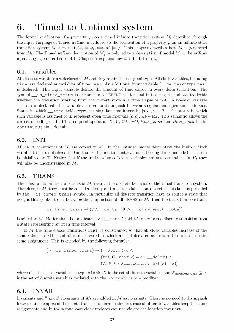
6. Timed to Untimed systemThe formal verification of a property ϕt on a timed infinite transition system Mt described throughthe input language of Timed nuXmv is reduced to the verification of a property ϕ on an infinite statetransition system M such that Mt |= ϕt ⇐⇒ M |= ϕ. This chapter describes how M is generatedfrom Mt. The Timed nuXmv description of Mf is reduced to a description of model M in the nuXmvinput language described in 4.1. Chapter 7 explains how ϕ is built from ϕt.

6.1. variablesAll discrete variables are declared inM and they retain their original type. All clock variables, includingtime, are declared as variables of type real. An additional input variable (__delta) of type realis declared. This input variable defines the amount of time elapse in every delta transition. Thesymbol __is_timed_trans is declared in a DEFINE section and it is a flag that allows to decidewhether the transition starting from the current state is a time elapse or not. A boolean variable__iota is declared, this variables is used to distinguish between singular and open time intervals.States in which __iota holds represent singular time intervals, [a; a], a ∈ R+, the states in whichsuch variable is assigned to ⊥ represent open time intervals (a, b), a, b ∈ R+. This semantic allows thecorrect encoding of the LTL temporal operators X, Y , @F , @O, time_since and time_until in thecontinuous time domain.

6.2. INITAll INIT constraints of Mt are copied in M . In the untimed model description the built-in clockvariable time is initialized to 0 and, since the first time interval must be singular to include 0, __iotais initialized to >. Notice that if the initial values of clock variables are not constrained in Mt theywill also be unconstrained in M .

6.3. TRANSThe constraints on the transitions of Mt restrict the discrete behavior of the timed transition system.Therefore, inM , they must be considered only on transitions labeled as discrete. This label is providedby the __is_timed_trans symbol, in particular all discrete transition have as source a state thatassigns this symbol to ⊥. Let ϕ be the conjunction of all TRANS in Mt, then the transition constraint

__is_timed_trans→ (ϕ ∧ __delta = 0 ∧ __iota ∧ next(__iota))

is added toM . Notice that the predicates over __iota forbidM to perform a discrete transition froma state representing an open time interval.

In M the time elapse transitions must be constrained so that all clock variables increase of thesame value __delta and all discrete variables which are not declared as noncontinuous keep thesame assignment. This is encoded by the following formula:

(¬__is_timed_trans)→ (__delta > 0 ∧(∀c ∈ C : next(c) = c+ __delta) ∧(∀x ∈ X \Xnoncontinuous : next(x) = x))

where C is the set of variables of type clock, X is the set of discrete variables and Xnoncontinuous ⊆ Xis the set of discrete variables declared with the noncontinuous modifier.

6.4. INVARInvariants and "timed" invariants of Mt are added in M as invariants. There is no need to distinguishbetween time elapses and discrete transitions since in the first case all discrete variables keep the sameassignments and in the second case clock updates can not violate the location invariant.

32

6.5. URGENTURGENT constraints in Mt define a list of sets of states in which time can not elapse. Let ϕ be theformula representing their union, computed as the disjunction of all such constraints. Since this formulacan contain both current and next variables it is encoded inM as a TRANS: ϕ→ __delta = 0. Thisforbids any time elapse transition from states in which ϕ holds.

33

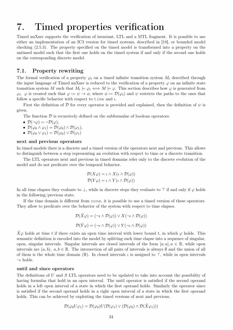
7. Timed properties verificationTimed nuXmv supports the verification of invariant, LTL and a MTL fragment. It is possible to useeither an implementation of an IC3 version for timed systems, described in [18], or bounded modelchecking (2.5.3). The property specified on the timed model is transformed into a property on theuntimed model such that the first one holds on the timed system if and only if the second one holdson the corresponding discrete model.

7.1. Property rewritingThe formal verification of a property ϕt on a timed infinite transition system Mt described throughthe input language of Timed nuXmv is reduced to the verification of a property ϕ on an infinite statetransition system M such that Mt |= ϕt ⇐⇒ M |= ϕ. This section describes how ϕ is generated fromϕt. ϕ is created such that ϕ ..= ψ → φ, where φ ..= D(ϕt) and ψ restricts the paths to the ones thatfollow a specific behavior with respect to time and ι.

First the definition of D for every operator is provided and explained, then the definition of ψ isgiven.

The function D is recursively defined on the subformulae of boolean operators:• D(¬ϕ) = ¬D(ϕ),• D(ϕ0 ∧ ϕ1) = D(ϕ0) ∧ D(ϕ1),• D(ϕ0 ∨ ϕ1) = D(ϕ0) ∨ D(ϕ1)

next and previous operatorsIn timed models there is a discrete and a timed version of the operators next and previous. This allowsto distinguish between a step representing an evolution with respect to time or a discrete transition.

The LTL operators next and previous in timed domains refer only to the discrete evolution of themodel and do not predicate over the temporal behavior.

D(Xϕ) = ι ∧X(ι ∧ D(ϕ))

D(Y ϕ) = ι ∧ Y (ι ∧ D(ϕ))

In all time elapses they evaluate to ⊥, while in discrete steps they evaluate to > if and only if ϕ holdsin the following/previous state.

If the time domain is different from none, it is possible to use a timed version of these operators.They allow to predicate over the behavior of the system with respect to time elapses.

D(Xϕ) = (¬ι ∧ D(ϕ)) ∨X(¬ι ∧ D(ϕ))

D(Y ϕ) = (¬ι ∧ D(ϕ)) ∨ Y (¬ι ∧ D(ϕ))

Xϕ holds at time t if there exists an open time interval with lower bound t, in which ϕ holds. Thissemantic definition is encoded into the model by splitting each time elapse into a sequence of singular,open, singular intervals. Singular intervals are closed intervals of the form [a; a], a ∈ R, while openintervals are (a, b), a, b ∈ R. The intersection of all pairs of intervals is always ∅ and the union of allof them is the whole time domain (R). In closed intervals ι is assigned to >, while in open intervals¬ι holds.

until and since operatorsThe definitions of U and S LTL operators need to be updated to take into account the possibility ofhaving formulas that hold in an open interval. The until operator is satisfied if the second operandholds in a left open interval of a state in which the first operand holds. Similarly the operator sinceis satisfied if the second operand holds in a right open interval of a state in which the first operandholds. This can be achieved by exploiting the timed versions of next and previous.

D(ϕ0Uϕ1) = D(ϕ0)U(D(ϕ1) ∨ (D(ϕ0) ∧ D(Xϕ1)))

34

D(ϕ0Sϕ1) = D(ϕ0)S(D(ϕ1) ∨ (D(ϕ0) ∧ D(Y ϕ1)))

All other LTL temporal operators can be expressed as a combination of U , S and ¬.

at next and at lastThe operators @F and @O in continuous timed systems must take into account that ϕ might hold inan open interval and therefore there might not be t ∈ Q : π, t |= ϕ even if Fϕ holds.

D(u@Fϕ) =

{D(u) if D(Xϕ)

D(u)@F (D(ϕ) ∨X(¬ι ∧ D(ϕ)) otherwise

D(u@Oϕ) =

{D(u) if D(Y ϕ)

D(u)@Y (D(ϕ) ∨ Y (¬ι ∧ D(ϕ)) otherwise

Notice that these operators in the timed case are rewritten using their semantic in the discrete model.u@Fϕ evaluates to the current value of u if in the open interval following the current state ϕ holds.Otherwise its value is the one assigned to u the first time that ϕ holds in either an open or closedinterval. The u@Oϕ case is symmetric, it refers to the past instead of the future.

at next, at last in untimed models. In discrete models for each distinct occurrence of theseoperators a new monitor variable is introduced to represent their value. Let m be a new symbol andu@Fϕ a LTL subformula. The following constraints are added for m:

1. ϕ → m = u, when the formula holds the monitor variable must correctly represent the value ofu.

2. next(m) 6= m→ ϕ, the value assigned to the monitor variable can change only right after ϕ held.These two constraints force m to assume the value that u will have the next time that ϕ will hold,since it can only change after a state that satisfies ϕ and in that state its value should match the oneof u.

Similarly for u@Oϕ, it is sufficient to replace the second constraint with next(m) 6= m→ next(ϕ).This forces the monitor to change value only before a state in which ϕ holds.

time since and time untilIn the input language the built-in variable time can only be used in comparison operations. Theoperators time_since and time_until allow to express an additional type of formulae.

D(time_since(ϕ)) = D(time)−D(time@Oϕ)

D(time_until(ϕ)) = D(time@Fϕ)−D(time)

These operators allow to predicate over the amount of time that passes between occurrences of ϕ.Notice that the formulae on the right side are not directly expressible in the input language.

time and iota constraintsThis section provides the additional constraints of time and ι. ψ ..= ψι∧ψtime, where ψtime forces theuniformity of time in open intervals for all predicates and ψι defines the alternation between singularand open intervals.

Let Subtime(ϕ) be the set of atomic predicates containing time. The input language restricts suchpredicates to be in the form time ./ u, u ∈ R ∧ ./∈ {<,≤, >,≥}. Then ψtime is defined as:

ψtime ..=∧

time./u∈Subtime(ϕ)

G(¬ι→ (D(time ≤ u)→ XD(time ≤ u)) ∧

(D(time ≥ u)→ XD(time ≥ u)))

The definition ψι depends on the type of the property, if the property is an invariant (INVARSPEC),then it can not contain any temporal operator. This allows to simplify the model behavior by avoiding

35

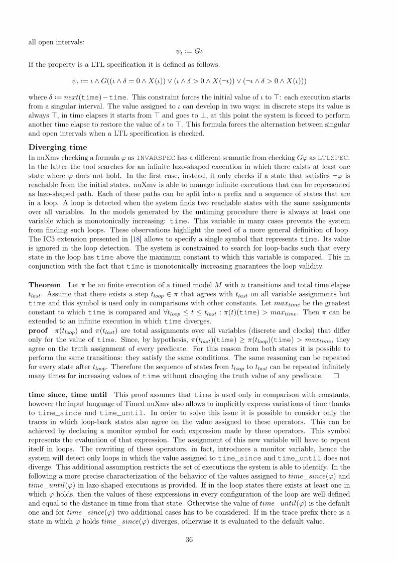
all open intervals:ψι ..= Gι

If the property is a LTL specification it is defined as follows:

ψι ..= ι ∧G((ι ∧ δ = 0 ∧X(ι)) ∨ (ι ∧ δ > 0 ∧X(¬ι)) ∨ (¬ι ∧ δ > 0 ∧X(ι)))

where δ ..= next(time)−time. This constraint forces the initial value of ι to >: each execution startsfrom a singular interval. The value assigned to ι can develop in two ways: in discrete steps its value isalways >, in time elapses it starts from > and goes to ⊥, at this point the system is forced to performanother time elapse to restore the value of ι to >. This formula forces the alternation between singularand open intervals when a LTL specification is checked.

Diverging timeIn nuXmv checking a formula ϕ as INVARSPEC has a different semantic from checking Gϕ as LTLSPEC.In the latter the tool searches for an infinite lazo-shaped execution in which there exists at least onestate where ϕ does not hold. In the first case, instead, it only checks if a state that satisfies ¬ϕ isreachable from the initial states. nuXmv is able to manage infinite executions that can be representedas lazo-shaped path. Each of these paths can be split into a prefix and a sequence of states that arein a loop. A loop is detected when the system finds two reachable states with the same assignmentsover all variables. In the models generated by the untiming procedure there is always at least onevariable which is monotonically increasing: time. This variable in many cases prevents the systemfrom finding such loops. These observations highlight the need of a more general definition of loop.The IC3 extension presented in [18] allows to specify a single symbol that represents time. Its valueis ignored in the loop detection. The system is constrained to search for loop-backs such that everystate in the loop has time above the maximum constant to which this variable is compared. This inconjunction with the fact that time is monotonically increasing guarantees the loop validity.

Theorem Let π be an finite execution of a timed model M with n transitions and total time elapsetlast. Assume that there exists a step tloop ∈ π that agrees with tlast on all variable assignments buttime and this symbol is used only in comparisons with other constants. Let maxtime be the greatestconstant to which time is compared and ∀tloop ≤ t ≤ tlast : π(t)(time) > maxtime. Then π can beextended to an infinite execution in which time diverges.proof π(tloop) and π(tlast) are total assignments over all variables (discrete and clocks) that differonly for the value of time. Since, by hypothesis, π(tlast)(time) ≥ π(tloop)(time) > maxtime, theyagree on the truth assignment of every predicate. For this reason from both states it is possible toperform the same transitions: they satisfy the same conditions. The same reasoning can be repeatedfor every state after tloop. Therefore the sequence of states from tloop to tlast can be repeated infinitelymany times for increasing values of time without changing the truth value of any predicate.

time since, time until This proof assumes that time is used only in comparison with constants,however the input language of Timed nuXmv also allows to implicitly express variations of time thanksto time_since and time_until. In order to solve this issue it is possible to consider only thetraces in which loop-back states also agree on the value assigned to these operators. This can beachieved by declaring a monitor symbol for each expression made by these operators. This symbolrepresents the evaluation of that expression. The assignment of this new variable will have to repeatitself in loops. The rewriting of these operators, in fact, introduces a monitor variable, hence thesystem will detect only loops in which the value assigned to time_since and time_until does notdiverge. This additional assumption restricts the set of executions the system is able to identify. In thefollowing a more precise characterization of the behavior of the values assigned to time_since(ϕ) andtime_until(ϕ) in lazo-shaped executions is provided. If in the loop states there exists at least one inwhich ϕ holds, then the values of these expressions in every configuration of the loop are well-definedand equal to the distance in time from that state. Otherwise the value of time_until(ϕ) is the defaultone and for time_since(ϕ) two additional cases has to be considered. If in the trace prefix there is astate in which ϕ holds time_since(ϕ) diverges, otherwise it is evaluated to the default value.

36

8. Timed tracesThis chapter describes how nuXmv traces have been extended to better represent executions of timedtransition systems. The first section describes how the expressiveness of the trace representation hasbeen improved. The following sections show how the simulation, execution and completion operationsare achieved for the new trace representation. Finally, the procedure to lift the discrete counter-exampleto a timed one is described.

8.1. RepresentationnuXmv traces allow to represent finite or lazo-shaped executions of an infinite discrete transitionsystem. It is not possible to represent any kind of infinite execution that is not lazo-shaped. In thesetraces the loop-back state is a configuration that agrees with the last state of the trace on the assignmentof all variables. This trace definition is not expressive enough to represent infinite executions of timedtransition system. Every infinite timed trace, by construction, has at least one diverging variable whichis time. From these observations the need to devise a more expressive representation becomes evident.The main objective of this section is the description of such new representation.

This issue is a particular instance of a more general problem, which is the representation of nonlazo-shaped behaviors in infinite transition systems. For this reason the problem is addressed in thediscrete case and then the solution is also adopted in the timed environment. This work proposes asolution which is expressive enough to represent timed traces, but also useful to address some specificcases of the more general instance. The proposed technique does not allow to represent arbitraryinfinite behaviors, but only a very specific subset of them.

Discrete Infinite TraceInfinite traces enrich nuXmv traces with a set of diverging variables. The symbols in this set are allowedto diverge in loops. The notion of loop is redefined so that the assignment of the last and loop-backstate must agree on the assignment of all symbols not in the diverging set. Every state in the traceloop associates every diverging symbol to an expression which is function of the previous value of thesame symbol. This defines a recurrence relation for each diverging variable, where the base condition isgiven by the value assigned to these variables in the last state outside of the loop. In this way, given aposition inside the loop and an iteration number, the value assigned to all symbols is well-defined. Moreformally, an infinite trace over a set of non-diverging symbols X and diverging variables D is a finitesequence of assignments π ..= s0, s1, . . . , sk over X ∪D such that ∃0 < l < k ∀x ∈ X : sl(x) = sk(x).sl, called loop-back state, agrees with sk on the assignment of all non diverging variables in X. For allstates not in a loop there is no distinction between variables in X and D: all of them are associatedto a concrete constant value. Each state in the loop, instead, associates to every diverging variable afunction that given the previous value of that variable returns its current value:

∀d ∈ D, l < j ≤ k ∃f ∈ type(d)2 : sj(d) = f(d)

where type(d) is the domain of the symbol d and f(x) = y ⇐⇒ (x, y) ∈ f . Notice that these recurrencerelations can refer to non-diverging symbols, upon evaluation they are simply replaced with the valueassigned to them in the previous step.

It is possible to iterate over infinite traces in two different modes. One mode allows to unroll theinfinite execution and builds the concrete assignments for every state by evaluating the recurrencerelation of the diverging symbols. The other mode is more complex: it tries to solve the recurrencerelation of every diverging symbol to obtain a closed form solution as a function of the iterationnumber. The closed form of the recurrence relations is exploited to perform operation on infinite traces:simulation, execution and completion. Currently only the very simple case in which the divergingvariable is updated by adding a constant value is handled. It could be possible to rely on externalprocedures to compute the closed form of such recurrence relations, however this solution has not beenexplored yet. Notice that this component is the only one that makes assumptions on the shape of therecurrence relation.

37

Timed traceA timed trace is an infinite trace where the built-in clock variable time is always in the set of divergingvariables: time ∈ D. The recurrence relation for this symbol is identical in every state of the loopand is given by timecurr = timeprev + δprev, where δ is the variable representing the amount of timeelapse and it is associated to a, possibly different, actual value in every state. Similarly all clockvariables that, inside the loop, are never reset are in the diverging set and they are assigned to thesame recurrence relation as time.

Notice that model checking on infinite transition systems and therefore also on timed transitionsystems is undecidable in its general formulation. For this reason, while soundness remains a necessarycondition, completeness of the proposed techniques can not be achieved. This observation motivatesthe restrictions made on the traces that can be represented in the system.

8.2. SimulationThis section explains how the formulation presented in 4.3.1 has been modified to implement thesimulation functionality for timed models.The simulation can be performed either automatically or interactively on a timed transition systemM ..= (S, I,N, T ). In automatic mode the system tries to build a finite, non-looping, trace of the modelof a specified length. This is achieved by appending one configuration at a time. The initial state ofthe trace is chosen among the ones that satisfy:

I ∧N

Every non-initial configuration is retrieved by a SMT call to check the satisfiability of:

s ∧N ∧ T

where s encodes the total assignment of the last configuration of the current trace. This is repeateduntil either a trace of the desired length has been built or the formula becomes unsatisfiable, in whichcase the simulation has reached a dead-lock state.

In interactive mode first the user has to choose the initial state from a list. The list is computedin the very same way as in nuXmv trance (4.3.1); the ith configuration is computed as the assignmentsatisfying:

I ∧N ∧i−1∧j=0

¬sj

where s0, . . . , si−1 are the total assignments that have been already found. Then the user can chooseif the system should perform a discrete transition or a time elapse. The configuration to be added tothe trace among the states that satisfy:

s ∧ δ > 0 ∧ T ∧N ′ ∧i−1∧j=0

¬s′j

if a time elapse has been requested,

s ∧ δ = 0 ∧ T ∧N ′ ∧i−1∧j=0

¬s′j

if the user asked for a discrete transition.

8.3. ExecutionThis section explains how the formulation presented in 4.3.2 has been modified to implement theexecution functionality for infinite, possibly timed, traces.Traces without loop-back state and configurations that do not belong to the trace loop can be handled

38

in the same way explained in 4.3.2. In these cases a state and its successor are total assignments thatassociate to every symbol a concrete constant value. The consistency of the trace initial state can beeasily verified by checking the satisfiability of the following formula:

s0 ∧ I ∧N

where s0 is the first state of the trace. For every configuration si : 0 ≤ i < l, where sl is the loop-backstate or the last configuration of the trace if no loop exists, the formula:

si ∧ s′i+1 ∧ T ∧N ′

must be satisfiable.

At this point the transitions between states in the loop and the loop itself must be checked for con-sistency with the infinite [timed] transition system. The procedure showed in 4.3.3 it is not applicablein this case. The new representation requires to prove that the recurrence relations assigned to thediverging symbols in the loop states allow the transition system to perform infinitely many iterations.Therefore, it is necessary to prove that the loop of the infinite trace is a valid representation of aninfinite execution of the infinite [timed] transition system.

Let π ..= s0, . . . , sl, . . . , sk be a trace of length k with loop-back state sl. Assume that eachassignment sj for l < j ≤ k associates to every diverging symbol the closed form solution of itsrecurrence relation as a function of iloop. iloop is a new symbol that represents the loop iterationnumber. The objective is to prove that for every iloop ∈ N each transition in the loop is valid and thatit is possible to perform a transition from s

iloopk to siloop+1

l+1 : from the last configuration of the trace atiteration iloop it is possible to reach the first loop state and begin iteration iloop + 1 for every iloop.

∀iloop ∈ N [(∀l ≤ j < k : (siloopj ∧ siloopj+1 )→ (T ∧Nj+1)) ∧ ((s

iloopk ∧ siloop+1

l+1 )→ (T ∧Nl+1))] (8.1)

To prove the validity of this formula it is possible to check the unsatisfiability of its negation using anSMT solver. Notice that each conjunct encodes the validity of one of the transitions in the loop, thelast cube verifies that it is always possible to begin the next iteration. By negating 8.1 it is possibleto obtain:

∃iloop ∈ N [∃l ≤ j < k : (siloopj ∧ siloopj+1 ∨ ¬T ∨ ¬Nj+1) ∨ (s

iloopk ∧ siloop+1

l+1 ∨ ¬T ∨ ¬Nl+1)] (8.2)

the loop defined by states sl, . . . , sk is valid in the transition system M if this last SMT formula (8.2)is unsatisfiable. In the case in which a satisfying model is found, such model assigns to iloop a loopiteration number for which it is not possible to perform one of the transitions. Moreover, by asking theSMT solver to prove the unsatisfiability of each disjunct one at a time it is also possible to preciselyidentify the transition of the loop that violates the behavior prescribed by the transition system.

8.4. Completion

This section explains how the formulation presented in 4.3.3 has been modified to implement thecompletion functionality for infinite, possibly timed, traces.The completion is supported only with respect to non diverging symbols; the complete informationabout the loop and the set of diverging symbols and all their recurrence relations must be provided. Asin the execution case (8.3), the same procedure explained in 4.3.3 is applied to perform the completionof the partial assignments that do not belong to the loop.

Consider the partial assignments in the trace loop: sl, ldots, sk. It is necessary to complete theirassignment so that the loop can be repeated infinitely many times. Let completes(s, s′) hold if andonly if the total assignment s is a completion of the partial assignment s′: they agree on all valuesof non-diverging symbols and assign the same recurrence relations to diverging symbols. Then it is

39

necessary to find a trace such that:

∃s′l, . . . , s′k :k∧j=l

completes(s′j , sj) ∧

∀iloop ∈ N [ (∀l ≤ j < k : (s′ iloopj ∧ s′ iloopj+1 )→ (T ∧Nj+1)) ∧

∀iloop ∈ N [ ((s′ iloopk ∧ s′ iloop+1

l+1 )→ (T ∧Nl+1)) ]

(8.3)

Notice that the second part is exactly the formula 8.1 on the existentially quantified completed assign-ments. The nesting of the different quantifiers (existential and universal) makes this formulation muchmore complex with respect to the one obtained in the execution case. In more detail, considering thepropositional case, the formulation showed in 8.1 belongs to the complexity class Π1 = co-NP whileformula 8.3 is an instance of Σ2. In the general SMT formulation their decidability is conditioned tothe decidability of the underlying theories.

Given this observation the decision taken in this work is to avoid the complexity of a completeapproach in favor of a more tractable, sound but incomplete procedure. In order to do this it isnecessary to remove the outer existential quantification. One possibility is to replace the existentialquantification with a universal one. This formulation would check that every possible completion of thetrace loop is valid, therefore the completion would succeed only in such cases. Another approach is topick one among the possible completions and check if the resulting completed trace is valid. This canbe achieved using the execution procedure described in 8.3. This second procedure has the advantageof being much simpler and correctly handles all cases handled by the first one.

8.5. From discrete to timed counter-exampleAs described in chapters 6 and 7, in this work the model checking problem on timed transition systemsis reduced to the one on discrete infinite transition systems. This reduction implies that the resultobtained in the discrete context has to be mapped back into the timed environment. If the property hasbeen verified, then the timed property also holds on the timed transition system. If the specificationis violated in the discrete system, the model checking procedure provides a counter-example: a traceof the discrete model in which the property does not hold. This trace has to be mapped into acorresponding execution of the timed system that proves that the timed specification does not hold.

Given an total assignment in the discrete trace, the corresponding total assignment of the timedtrace is built by coping the value assigned to all symbols that belong to both discrete and timedtransition system. A transition of the discrete trace is mapped into either a discrete or time elapsebased on the value assigned to δ in the source configuration. If δ = 0 then the transition is a discreteone, otherwise it is a time elapse. From the property rewriting (7.1) it is possible to notice that thereare three possible kinds of time elapses between two configurations s0 and s1:

1. s0 |= ι and s1 |= ι: in this case both states represent singular intervals;2. s0 |= ι and s1 |= ¬ι: in this case s0 represents a singular interval, while s1 represents a time

instant in an open interval;3. s0 |= ¬ι and s1 |= ι: in this case s0 represents a time instant in an open interval, while s1

represents a singular interval;In all cases the states represent total assignments over the variables, therefore they can be representedas total assignments also in the timed trace. In the second and third case one of the states is used torepresent an open interval and in the trace it splits the left and right neighborhood of the previousand following configurations. In these neighborhoods temporal operators like X, Y , @F and @O areevaluated. For these reasons all these transitions are represented in the timed trace as a single timeelapses from s0 to s1.

40

9. Experimental evaluationThe techniques described so far have been implemented inside the workflow of the nuXmv symbolicmodel checker. This implementation is compared to other state-of-the-art model checkers for timedtransition system, which implement the main approaches described in chapter 3. This chapter firstprovides a description of the software to which Timed nuXmv is compared. Their descriptions arenot exhaustive, the objective is to provide a high level perspective of the features they support andtechniques they implement. Then a brief explanation of the testing environment is provided. Finallythe benchmarks models and obtained results are presented and commented.

9.1. Description of the toolsThis section briefly describes the model checkers Uppaal (9.1.1), ATMOC (9.1.2) and LTSmin (9.1.3).In 9.1.4 the verification algorithms used to evaluate Timed nuXmv are cited.

UppaalUppaal was released for the first time in 1995 and it is actively developed and maintained by theUppsala University and Aalborg University. Uppaal supports modeling, simulation and verification ofnetworks of timed automata extended with shared integer variables, urgent channels and committedlocations [7]. The formal verification of properties is based on the construction of the zone automa-ton (3.3) corresponding to the composition of the timed automata in the network. DBMs are usedto represent and execute transformations on zones [6]. Uppaal supports only bounded variable typesand therefore finite timed asynchronous transition systems. The additional constructs: shared inte-ger variables, urgent channels and committed locations provide some synchronization primitives. Inparticular: shared integer variables allow for asynchronous communication between processes, urgentchannels force the system to perform a certain transition as soon as the transition is enabled andcommitted locations allow to define a sequence of action to be performed atomically without delaysor interference of the other processes. The specification language supported by Uppaal is a subset ofTCTL [12][13]:

ϕ :: AGψ | EGψ | AFψ | EFψ | ψ 99K φ

where ψ 99K φ is equivalent to AG(φ → AFψ) and ψ and φ are propositional logic predicates overstate variables, locations, shared variables and clock constraints in B(X).

Uppaal is split into two main components: a graphical user interface that helps in the definitionof the timed automata network and a verification engine that given a xml network description and aspecification checks if such network satisfies the property. The verification engine searches for a pathin the zone automaton that starts from an initial state and ends in a state such that its location is afinal one and its clock assignments satisfy the property [8].

Algorithm 1 Timed automata reachability algorithm1: procedure Reachable((l0, D0), (lf , φf ), k) . initial and final states, maximal constant2: passed← ∅ . set of explored states3: wait← {(l0, D0)} . states to be explored4: while wait 6= ∅ do . until there is nothing more to visit5: (l,D)← wait.pop() . extract one element from list6: if l = lf ∧D ∩ φf 6= ∅ then . final states and clocks satisfy the constraints7: return >8: if ∀(l,D′) ∈ passed : D 6⊆ D′ then . current state not already included by other visited9: passed← passed ∪ (l,D) . update set of visited states

10: for all (l′, D′) : (l,D) k,G (l′, D′) do11: wait← wait ∪ (l′, D′) . add set of states reachable from (l,D)

12: return ⊥ . explored all states, not reached

The algorithm 1 is a simplified version of the reachability algorithm implemented in Uppaal [6].

41

In particular many optimization are omitted, like the usage of a specialized data structure instead ofthe two sets passed and wait. Line 8 checks if among the states that have already been visited withlocation l, there is one that has a clock interpretation that subsumes the current one; in this case itis not necessary to update the list of visited states, since the current state is already represented. Inline 10 the algorithm iterates over all states reachable from the current one by performing a transitionwith delay at most k and subjected to the difference clock constraints G of the automaton and theproperty. The termination of procedure 1 is guaranteed by the fact that the regions are finitely manyand their power set imposes an upper bound on the number of zones. Therefore, k,G is finite andeventually all possible states will be visited.

The description of the Uppaal GUI is out of the scope of this work, for an introduction on itsfeatures and usage refer to [7].

ATMOC

The Aalto Timed Model Checker (ATMOC) is a symbolic timed model checker developed in 2012 byRoland Kindermann, Tommi Junttila and Ilkka Niemelä. The tool implements the techniques theydescribe in [25]: an extension of IC3 (2.5.3) and K-induction (2.5.3) to deal with symbolic timedtransition systems (STTS). ATMOC supports the verification of invariant specifications on a modeldescription. From the input model ATMOC implicitly generates the symbolic representation of theregion abstracted machine (3.2) to obtain a finite state representation of the STTS.

K-induction ATMOC adds an additional constraint on the K-induction paths: no two states ofeach path can belong to the same region. This is done symbolically by constraining the integral andfractional part of the clock interpretations. In this way the K-induction technique is forced to lookonly at paths that visit at most one state for each region [25]. The following formula constrains twostates indexed by i, j to belong to different regions:∨

x∈Xx[i] 6= x[j] ∨ (9.1a)∨

c∈C(c

[i]int 6= c

[j]int ∧ (¬max[i]c ∨ ¬max[j]c )) ∨ (9.1b)∨

c∈C(¬max[i]c ∧ ¬(c

[i]fract = 0 ⇐⇒ c

[j]fract = 0)) ∨ (9.1c)∨

c∈C

∨d∈C\{c}

(¬max[i]c ∧ ¬max[i]d ∧ ¬(c

[i]fract ≤ d

[i]fract ⇐⇒ c

[j]fract ≤ d

[j]fract)) (9.1d)

whereX is the set of discrete (non clock) variables, C is the set of clocks, c[i]int is the integral part of clockc at state i, c[i]fract is the fractional part of clock c at state i, max

[i]c

..= c[i]int > mc∨(c

[i]int = mc∧cfract > 0)

and mc is the maximum constant to which c is compared.

This formulation can be more easily understood by looking at the matrix representation of regionsshown in figure 3.1. The clause 9.1a encodes that if the two states disagree on the assignment of atleast one discrete variable then they belong to different regions. 9.1b ensures that if in both states c iswithin its maximum relevant value and the integral part is different then they can not be in the sameregion. The clause 9.1c distinguishes between the regions that assign to c a value in Z and the onesthat have fractional part different from 0. The subformula 9.1d checks that for every pair of distinctclocks they do not belong to the same side of the "diagonals".

IC3 A similar approach is taken to extend IC3 (2.5.3) to handle STTS [25]. As in the previous casethe objective is to lift the procedure to reason on the region abstraction. This is achieved by replacingin every SMT call each concrete state with a representation of its region. Given a state s its region

42

representation s is built so that for every state µ in the same region of s: µ |= s.

s ..=∧x∈X

x = s(x) ∧ (9.2a)∧c∈C:s(c)>mc

c > mc ∧ (9.2b)

∧c∈C:s(c)≤mc

{c = s(c) if fract(s(c)) = 0

c < ds(c)e ∧ c > bs(c)c if fract(s(c)) 6= 0∧ (9.2c)

∧c∈C:s(c)≤mc

∧d∈C\{c}:s(d)≤md

d = fract(s(c)) + bs(d)c, if fract(s(c)) = fract(s(d))

d > fract(s(c)) + bs(d)c, if fract(s(c)) < fract(s(d))

c > fract(s(d)) + bs(c)c, if fract(s(c)) > fract(s(d))

(9.2d)

where X is the set of discrete variables, C is the set of clocks, s(c) is the interpretation of variable c atstate s, mc is the maximum value to which the clock variable c is compared and fract(k) ..= k − bkc.

Formula 9.2 is built using the same observations done for 9.1. However, the latter encodes the factthat two states belong to different regions while the first one creates a symbolic representation of aregion given one of the states in it. As in the previous case the visualization of regions shown in 3.1might provide a better intuition. The cube 9.2a encodes the fact that all states in the same regionmust agree on the assignment over the discrete variables, this is the negation of the clause 9.1a. Theconstraint 9.2b ensures that all states agree on the set of clock variables assigned to values above theirmaximum relevant value. The cube 9.2c is the negation of clause 9.1b. It encodes the fact that allstates in the same region of s have the same integral part and if s(c) ∈ Z they have exactly the samevalue for every clock variable that does not exceed the maximum relevant value. The subformula 9.2dconstrains the relationship between the fractional parts of clock assignments for states in the sameregion. The formulation is similar to clauses 9.1c and 9.1d: the assignment of every pair of clocks lieson, above or below the "diagonal".

In the IC3 version just described the generalization procedure is applied to s instead of s andequation 2.2 becomes:

Fi−1 ∧ ¬s ∧ T ∧ s′ (9.3)

Further optimization of these techniques is possible by noticing that if a region is unreachable thenalso all its time-predecessor regions are. This observation allows ATMOC to exclude more regions ata time [25].

In a later work [24] Kindermann, Junttila and Niemelä extend this approach to support also theverification of a fragment of MTL, called MITL0,+∞, on timed automata using bounded model checking.Timed nuXmv supports the same fragment, their performance are compared on the benchmark usedin [24].

LTSminLTSmin is a model checker for labeled transition systems developed by the University of Twente. Itis characterized by a highly modular structure; there are three main components: a language front-end, a simplification module and an algorithmic back-end [27]. Each of this components relies on aunifying interface called Partitioned Next-State Interface (PINS). The language front-end parses theinput model and specification from some formal specification language (like the Uppaal language)and encodes it using the structures provided by PINS. The simplification module consists of a setof functions that perform transformations on the PINS structures to obtain an equivalent but morecompact representation. The algorithmic backend can be one of some already provided engines or evenan external one. They take as input the PINS structure are perform the verification task [11].

A model described using PINS is a Partitioned Transition System (PTS) P ..= (SP ,→P , s0, L),where:

• SP = S1 × S2 × . . .× SN is the set of states, each state s ∈ Sp is a N ∈ N dimensional vector.

43

• →P

K⋃i=1→i is the labeled transition relation, it is composed by K transition groups

→i⊆ SP ×A× Sp, where A is the set of action labels.• s0 ∈ SP is the initial state.• L : SP × L 7→ N, where L is the set of state labels, is the state labeling function,

let L(s) ..= {l|L(s, l) 6= 0}.LTSmin allows to specify dependencies between the transition groups and slots of the state vector.These information allow the tool to extract some properties of the transition groups: read independence(every transition in the group is independent to the value of a particular slot), write independence (everytransition in the group does not modify the value of a particular slot) and label independence (the samelabel is assigned to states that differ for the value of a particular slot). Guards are associated to eachtransition group and not to single transitions [23].

LTSmin supports the language front-end of Uppaal through Opaal. Given a Uppaal model Opaalgenerates the corresponding C code that implements the PINS. Opaal creates the zone abstractionof the timed automaton which is encoded into a PTS and passed to the simplification module. Thismodule is able to check for subsumption relation between two states on-the-fly. This allows to prunethe PTS and reduce the size of the state space.

LTSmin supports LTL model checking through the LTL layer. This layer computes the Büchiautomaton corresponding to the negated formula. Then the product of the model and this automatonis computed on the fly. The resulting machine is given to the analysis algorithms that search for anaccepting cycle. If such cycle exists then the original property does not hold, otherwise the languageof the product machine is empty and the specification holds.

The tool provides different analysis back-ends and allows to specify different search strategies, someof which run multiple parallel visits. NDFS is the well known nested depth first search algorithm,CNDFS run multiple, synchronized depth first searches in parallel, DFSFIFO combines CNDFS withbreadth first search to detect livelocks [27].

Timed nuXmvTimed nuXmv can exploit all verification engines implemented in nuXmv, thanks to the reduction todiscrete infinite model checking described in chapters 6 and 7. The following paragraph reports theverification algorithms exposed by Timed nuXmv interface. For invariant verification it is possible toexploit an implementation of the IC3 extensions presented in paragraphs 2.5.3 and 2.5.3. The secondone is the default algorithm and the user can request the first one by specifying an additional commandline option that disables the implicit abstraction. For LTL and MTL checking Timed nuXmv allowsto choose between two algorithms: one is the extension of IC3 with implicit abstraction (2.5.3) andthe other one is based on bounded model checking (2.5.3).

9.2. Benchmarks and resultsThis section describes the benchmarks used to evaluate the different tools and shows the obtainedresults in terms of time and space required to perform a single model checking task. Unfortunately, inthe literature there are not many publicly available models suitable for timed systems and even lessfor synchronous systems. In this evaluation two popular benchmarks are used. The first one has beentaken from the Uppaal test suite, while the second one has been taken from the ATMOC examples.Timed nuXmv has been run using both algorithms for invariant verification: IC3 with and withoutimplicit abstraction.

Fischer mutual exclusion algorithmThe Fischer mutual exclusion algorithm was first proposed by Michael Fischer. A mutual exclusionalgorithm is a procedure that allows two or more processes to coordinate so that they access a sharedresource (critical section) one at a time. The fischer mutual exclusion is based on real-time assumptions:every process in the system has access to a synchronized clock. Every process that wants to accessthe critical section sets a shared variable id to 0, then it waits for at most c time units before settingid to its own pid; at this point the process has to wait at least c time units. If, after this amount oftime, the shared variable id is still equal to its own pid, then the process can safely enter in the critical

44

section, otherwise the procedure is repeated. c is a constant known to every process and should be anupper bound of the execution time between successive steps. The key component of this algorithm arethe delays. For this reason this procedure is widely used as a benchmark for timed automata modelchecking.

Algorithm 2 Fischer mutual exclusion1: procedure Fischer(pid, c, id) . process id, constant c, shared variable2: loop3: while id 6= 0 do . wait if someone else is trying to access CS4: skip

5: x← random(0, c) . random delay in the interval6: wait_at_most(c) . wait at most c before going on7: id← pid . process pid wants to access CS8: wait_at_least(c) . wait at least c before proceeding9: if id = pid then

10: Critical Section11: id← 0

This simple algorithm has been modeled in the input languages of Timed nuXmv, ATMOC andUppaal using c = 2. The language supported by Opaal is the same as Uppaal. It allows to specifya network of timed automata, therefore it allows to directly model the asynchronous composition ofthe different processes. The languages of Timed nuXmv and ATMOC are very similar, there aresome minor differences on the timed fragment of the syntax. Neither of these two languages providesspecialized elements to directly model asynchronous systems. For this reason it has been necessaryto embed an explicit scheduler in the model. The scheduler is an unconstrained variable that decideswhich process is allowed to perform a transition. All four model checkers are asked to prove themutual exclusion invariant property on systems with an increasing number of processes implementingthe Fischer protocol.

In [24] four MTL properties are used as benchmarks. In this work the very same properties areused to compare Timed nuXmv with the tool proposed in that publication. The first specification asksto prove that in the unbounded time interval [0,∞) if a process asks to access the critical section thenit eventually enters the waiting state. The second specification tries to prove that in the unboundedinterval [0,∞) there is no execution that visits infinitely often the critical section and the non-criticalsection. The third specification is the bounded version of the first one: it tries to prove that the processenters the wait state in at most 2 time units. The fourth and last specification is the bounded versionof the second one: it tries to prove that a process enters the critical section in at most 3 time units.

Results

This section shows the result obtained by measuring the performance in the verification of the invariantmutual exclusion property and the four MTL specifications on the Fischer protocol.

Invariant

These tests were executed on a machine running Ubuntu 16.04 and equipped with 16 GB RAMand as processor an Intel Xeon with a base frequency of 3.70 GHz. Each model checking task has beenexecuted with a time limit of 1 hour and 20 GB of maximum virtual memory. A job was stopped assoon as the execution exceeded one of these boundaries. Each model checker was asked to prove themutual exclusion property for an increasing number of processes: from 2 to 40.

45

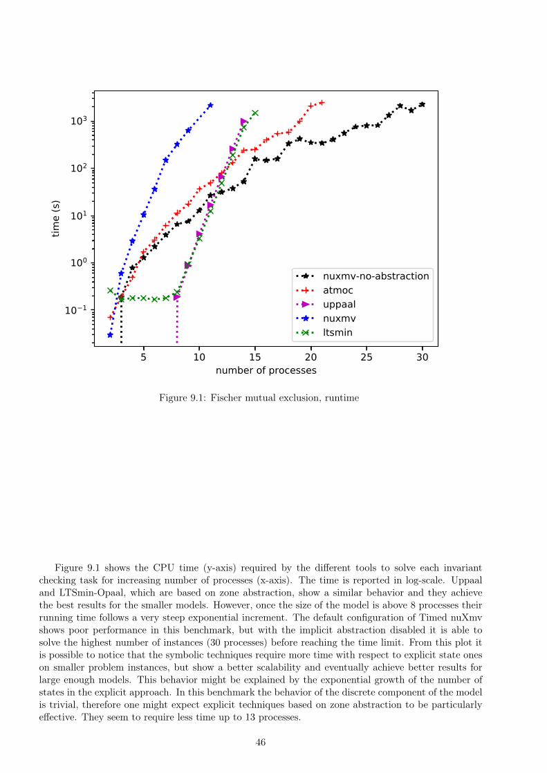
5 10 15 20 25 30number of processes

10 1

100

101

102

103

time

(s)

nuxmv-no-abstractionatmocuppaalnuxmvltsmin

Figure 9.1: Fischer mutual exclusion, runtime

Figure 9.1 shows the CPU time (y-axis) required by the different tools to solve each invariantchecking task for increasing number of processes (x-axis). The time is reported in log-scale. Uppaaland LTSmin-Opaal, which are based on zone abstraction, show a similar behavior and they achievethe best results for the smaller models. However, once the size of the model is above 8 processes theirrunning time follows a very steep exponential increment. The default configuration of Timed nuXmvshows poor performance in this benchmark, but with the implicit abstraction disabled it is able tosolve the highest number of instances (30 processes) before reaching the time limit. From this plot itis possible to notice that the symbolic techniques require more time with respect to explicit state oneson smaller problem instances, but show a better scalability and eventually achieve better results forlarge enough models. This behavior might be explained by the exponential growth of the number ofstates in the explicit approach. In this benchmark the behavior of the discrete component of the modelis trivial, therefore one might expect explicit techniques based on zone abstraction to be particularlyeffective. They seem to require less time up to 13 processes.

46

5 10 15 20 25 30number of processes

0

2000

4000

6000

8000

10000

12000

spac

e (M

B)

nuxmv-no-abstractionatmocuppaalnuxmvltsmin

Figure 9.2: Fischer mutual exclusion, memory usage

Figure 9.2 shows the resident memory (y-axis) required by the different tools to solve each invariantchecking task for an increasing number of processes (x-axis). All tools require a little amount ofmemory up to 8 processes. It is relevant to notice that none of the tools gets stopped due to a memoryout, but always because of the time limit. As for the runtime, also in this case, the behavior ofUppaal and LTSmin-Opaal are quite similar, with Uppaal being able to handle a few more instancesbefore the exponential increase of memory usage. Timed nuXmv without the implicit abstraction hasbetter memory performance with respect to Uppaal and LTSmin-Opaal for models with more than 12processes, notice that it also achieves better time performance after 13. ATMOC shows very smallmemory requirements, with an almost linear increase of about 2 MB for each additional process.

MTL

These tests executed on a machine running Fedora with Scientific Linux 7.3 and equipped with 46GB RAM and as processor an Intel Xeon with a base frequency of 2.50 GHz. Each model checkingtask has been executed with a time limit of 1 hour and 40 GB of maximum virtual memory. A job wasstopped as soon as the execution exceeded one of these boundaries. Each model checker was asked toprove one MTL property at a time for an increasing number of processes: from 2 to 20.

There are four MTL specifications:0. The first specification, identified by 0, asks to prove that in the unbounded time interval [0,∞)

if a process asks to access the critical section then it eventually enters the waiting state.

G(state = req → (F[0;∞) state = wait))

1. The second specification, identified by 1, tries to prove that there is no execution in which a

47

process enters infinitely often the non-critical sections and the critical in the unbounded interval[0,∞).

¬GF (state = idle ∧ (F[0,∞) state = cs))

2. The third specification, identified by 2, is the bounded version of the first one: it tries to provethat the process enters the wait state in at most 2 time units.

G(state = req → (F[0;2] state = wait))

3. The fourth and last specification, identified by 3, is the bounded version of the second one: ittries to prove that a process enters the critical section after at most 3 time units.

¬GF (state = idle ∧ (F[0,3] state = cs))

Timed nuXmv has been run using both algorithms available for MTL verification: one is based on IC3-IA (2.5.3) and the other based on BMC (2.5.3). Their running time and memory usage are comparedwith the ones achieved by the software described in [24], called ATMOC-mtlbmc.

2 4 6 8 10 12 14 16number of processes

101

102

103

time

(s)

nuxmv

(a) Fischer MTL property 0, runtime

2 4 6 8 10 12 14 16 18number of processes

101

102

103

time

(s)

nuxmv

(b) Fischer MTL property 2, runtime

Figure 9.3: Fischer true MTL properties, runtime

The plots in 9.3 show the time required to verify the properties with id 0 and 2. These specificationshold, therefore the BMC (2.5.3) based approaches, nuxmv-bmc and ATMOC-mtlbmc, are unable toterminate. The default algorithm of nuXmv, based on IC3, is able to give an answer. The requiredtime seems to increase as the number of processes increases however their dependency is not as clearas in the invariant checking case. Notice that in figure 9.3b the tool reaches the time limit for modelswith 6, 9, 13, 14, 15, 16 and 17 processes, while it is able to give an answer within this limit for 18.

48

2 4 6 8 10 12 14 16 18 20number of processes

10 1

100

101

102

103tim

e (s

)nuxmv-bmcnuxmvatmoc-mtlbmc

(a) Fischer MTL property 1, runtime

2 4 6 8 10 12 14 16 18 20number of processes

100

101

time

(s)

nuxmv-bmcnuxmvatmoc-mtlbmc

(b) Fischer MTL property 3, runtime

Figure 9.4: Fischer false MTL properties, runtime

Figure 9.4 shows the time required to find a counter-example for the properties with id 1 and 3. Thetwo algorithms of Timed nuXmv have a very similar behavior, while ATMOC-mtlbmc requires muchless time. Timed nuXmv is unable to obtain an answer for property 3 since the rewriting of the property(7.1) introduces some monitors for the time_since and time_until operators that diverge. Thiskind of behavior is not recognized at the moment and the procedure never halts (7.1.6). This mightalso be the cause for the additional time required to identify the counter-example to property 1. TimednuXmv is unable to consider all that executions, therefore it has to search for longer paths that violatethe property. ATMOC-mtlbmc is able to identify these behaviors thanks to the region abstraction,which can not be used by Timed nuXmv due to the additional expressiveness of its input language.

2 4 6 8 10 12 14 16number of processes

100

200

300

400

spac

e (M

B)

nuxmv

(a) Fischer MTL property 0, memory usage

2 4 6 8 10 12 14 16 18number of processes

50

100

150

200

250

300

350

400

450

spac

e (M

B)

nuxmv

(b) Fischer MTL property 2, memory usage

49

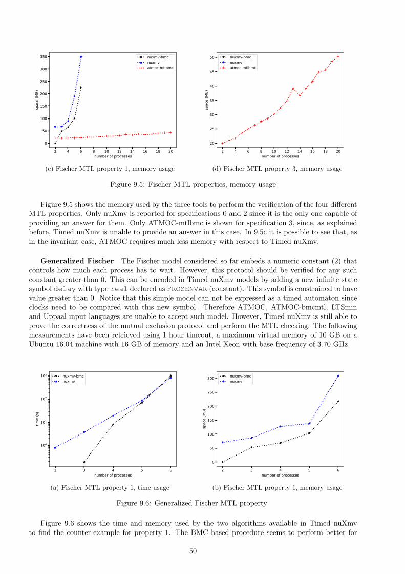
2 4 6 8 10 12 14 16 18 20number of processes

0

50

100

150

200

250

300

350

spac

e (M

B)

nuxmv-bmcnuxmvatmoc-mtlbmc

(c) Fischer MTL property 1, memory usage

2 4 6 8 10 12 14 16 18 20number of processes

20

25

30

35

40

45

50

spac

e (M

B)

nuxmv-bmcnuxmvatmoc-mtlbmc

(d) Fischer MTL property 3, memory usage

Figure 9.5: Fischer MTL properties, memory usage

Figure 9.5 shows the memory used by the three tools to perform the verification of the four differentMTL properties. Only nuXmv is reported for specifications 0 and 2 since it is the only one capable ofproviding an answer for them. Only ATMOC-mtlbmc is shown for specification 3, since, as explainedbefore, Timed nuXmv is unable to provide an answer in this case. In 9.5c it is possible to see that, asin the invariant case, ATMOC requires much less memory with respect to Timed nuXmv.

Generalized Fischer The Fischer model considered so far embeds a numeric constant (2) thatcontrols how much each process has to wait. However, this protocol should be verified for any suchconstant greater than 0. This can be encoded in Timed nuXmv models by adding a new infinite statesymbol delay with type real declared as FROZENVAR (constant). This symbol is constrained to havevalue greater than 0. Notice that this simple model can not be expressed as a timed automaton sinceclocks need to be compared with this new symbol. Therefore ATMOC, ATMOC-bmcmtl, LTSminand Uppaal input languages are unable to accept such model. However, Timed nuXmv is still able toprove the correctness of the mutual exclusion protocol and perform the MTL checking. The followingmeasurements have been retrieved using 1 hour timeout, a maximum virtual memory of 10 GB on aUbuntu 16.04 machine with 16 GB of memory and an Intel Xeon with base frequency of 3.70 GHz.

2 3 4 5 6number of processes

100

101

102

103

time

(s)

nuxmv-bmcnuxmv

(a) Fischer MTL property 1, time usage

2 3 4 5 6number of processes

0

50

100

150

200

250

300

spac

e (M

B)

nuxmv-bmcnuxmv

(b) Fischer MTL property 1, memory usage

Figure 9.6: Generalized Fischer MTL property

Figure 9.6 shows the time and memory used by the two algorithms available in Timed nuXmvto find the counter-example for property 1. The BMC based procedure seems to perform better for

50

smaller models and has smaller memory requirements.

2 4 6 8 10 12 14number of processes

10 1

100

101

102

103

time

(s)

nuxmvnuxmv-no-abstraction

(a) Fischer mutual exclusion property, time usage

2 4 6 8 10 12 14number of processes

0

1000

2000

3000

4000

spac

e (M

B)

nuxmvnuxmv-no-abstraction

(b) Fischer mutual exclusion property, memory usage

Figure 9.7: Generalized Fischer mutual exclusion properties

Figure 9.7 shows the time and memory required by Timed nuXmv to verify the mutual exclusionproperty. It is possible to notice that in this case the time out is reached for 15 processes while in theprevious case (9.1, 9.2) Timed nuXmv was able to provide an answer for all model with less than 31processes.

Diesel generatorThe diesel generator benchmark is an industrial model of an emergency diesel generator intendedfor the use in a nuclear power plant. The benchmark comes in three different sizes: small, mediumand large. The largest version represents the whole system and has 24 clock variables and 130 statevariables. The medium and smaller models represent only a subset of components which are sufficientto prove some of the properties. The medium sized has 7 clocks and 64 variables and the smallest 6clocks and 36 state variables. These models are not suitable to be represented explicitly, due to thehigh number of possible states. For this reason only the symbolic techniques have been applied. Eachmodel contains some properties, the tool is asked to verify one property at a time. The specificationsare all invariants since ATMOC does not support LTL verification. These models describe synchronouscomponents, therefore no explicit monitor is required.

Results

These tests were executed on a machine running Fedora with Scientific Linux 7.3 16.04 and equippedwith 46 GB RAM and as processor an Intel Xeon with a base frequency of 2.50 GHz. Each modelchecking task has been executed with a time limit of 2 hours and 40 GB of maximum virtual memory.A job was stopped as soon as the execution exceeded one of these boundaries. Each model checkerwas asked to prove one invariant property at a time for the three different sizes of the model.

property number ATMOC (s) nuXmv (s) nuXmv without abstraction (s)0 0.5 0.1 0.11 0.5 0.0 0.02 0.5 0.1 0.13 0.5 0.0 0.04 0.5 0.2 0.15 0.5 0.0 0.0

Table 9.1: diesel generator, small

51

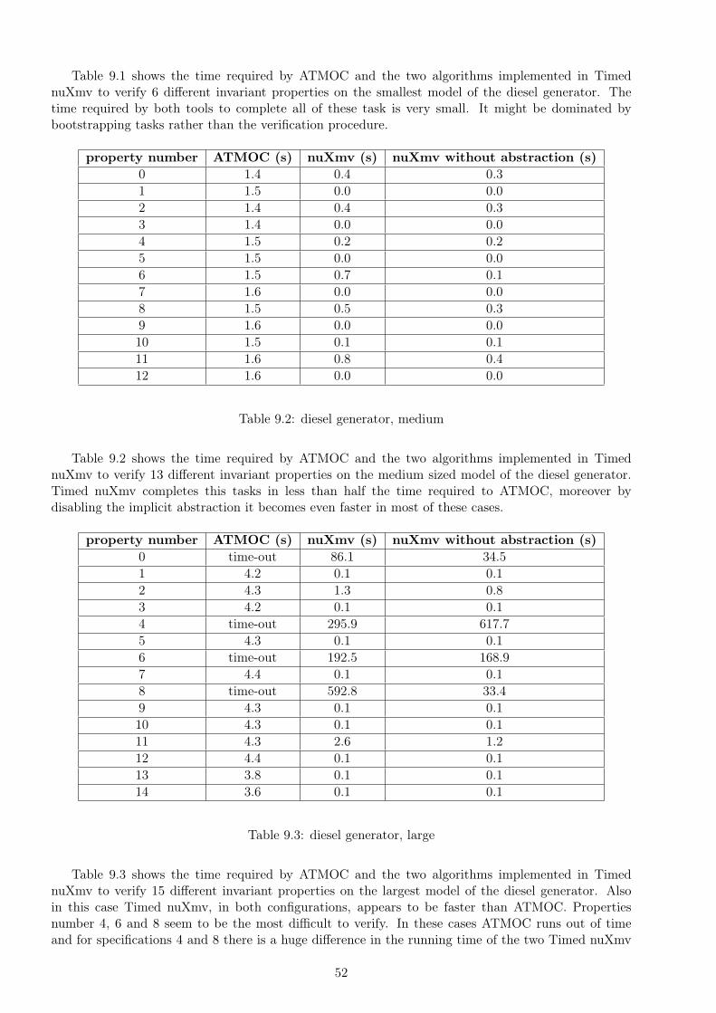
Table 9.1 shows the time required by ATMOC and the two algorithms implemented in TimednuXmv to verify 6 different invariant properties on the smallest model of the diesel generator. Thetime required by both tools to complete all of these task is very small. It might be dominated bybootstrapping tasks rather than the verification procedure.

property number ATMOC (s) nuXmv (s) nuXmv without abstraction (s)0 1.4 0.4 0.31 1.5 0.0 0.02 1.4 0.4 0.33 1.4 0.0 0.04 1.5 0.2 0.25 1.5 0.0 0.06 1.5 0.7 0.17 1.6 0.0 0.08 1.5 0.5 0.39 1.6 0.0 0.010 1.5 0.1 0.111 1.6 0.8 0.412 1.6 0.0 0.0

Table 9.2: diesel generator, medium

Table 9.2 shows the time required by ATMOC and the two algorithms implemented in TimednuXmv to verify 13 different invariant properties on the medium sized model of the diesel generator.Timed nuXmv completes this tasks in less than half the time required to ATMOC, moreover bydisabling the implicit abstraction it becomes even faster in most of these cases.

property number ATMOC (s) nuXmv (s) nuXmv without abstraction (s)0 time-out 86.1 34.51 4.2 0.1 0.12 4.3 1.3 0.83 4.2 0.1 0.14 time-out 295.9 617.75 4.3 0.1 0.16 time-out 192.5 168.97 4.4 0.1 0.18 time-out 592.8 33.49 4.3 0.1 0.110 4.3 0.1 0.111 4.3 2.6 1.212 4.4 0.1 0.113 3.8 0.1 0.114 3.6 0.1 0.1

Table 9.3: diesel generator, large

Table 9.3 shows the time required by ATMOC and the two algorithms implemented in TimednuXmv to verify 15 different invariant properties on the largest model of the diesel generator. Alsoin this case Timed nuXmv, in both configurations, appears to be faster than ATMOC. Propertiesnumber 4, 6 and 8 seem to be the most difficult to verify. In these cases ATMOC runs out of timeand for specifications 4 and 8 there is a huge difference in the running time of the two Timed nuXmv

52

configurations. The default one is much faster in property 4, while by removing the implicit abstractionthe time required to verify property 8 is reduced by one order of magnitude.

These experimental results highlight that the technique designed and implemented in this workis at least competitive with some state-of-the-art tools. It is relevant to notice that most of thesecomparisons have been performed on systems representable as timed automata, while Timed nuXmvsupports the verification of a more general form of timed transition systems. Most of the consideredproperties were invariant since there is little support for generalized LTL and MTL model checking ontimed transition systems. The Fischer benchmarks highlighted that the default configuration of TimednuXmv sometimes leads to poor performance. In this cases a little exploration of different possibleconfigurations might lead to much better results.

53

10. ConclusionsThis work presented and explained the new features implemented in the nuXmv symbolic modelchecker. The contribution of this thesis can be summarized in six main different aspects:

1. language definition (chapter 5),2. model compilation and reduction (chapter 6),3. verification of properties (chapter 7),4. system simulation (section 8.2),5. definition and representation of infinite traces (section 8.1),6. trace execution and completion (sections 8.3 and 8.4).

Together they led to the development of a new version of the software called Timed nuXmv. Thisnew version is fully backward compatible and extends all high-level functionalities available in nuXmvto the timed case. The tool is now able to handle the formal verification of invariant, LTL andMTL specifications over timed transition systems expressed in an extension of the smv language. Theadditional expressiveness of the Timed nuXmv input language, with respect to other state-of-the-arttools, does not allow to rely on the region and zone abstraction of the time behavior. However, asshown in chapter 9, the performance in terms of execution time and memory usage are comparablewith other model checkers for real-time systems. Among all the tools analyzed, in these benchmarks,Timed nuXmv shows the best scalability in reachability analysis. It has the ability of proving positiveresults for MTL specifications, however, for negative results, it suffers from the limited capacity toidentify and represent diverging variables.

10.1. Future workThis section briefly discusses some possible further developments of the work presented in this thesis:Timed nuXmv. The extensions can be organized in five main possible directions. Each of the followingparagraphs analyses one of them.

Language constraintsThe language of Timed nuXmv, while more expressive then the one of timed automata, still hassome limitations (chapter 5). A possible future development would be to relax some of them. Forexample: allowing non-convex invariant conditions, the usage of clocks in specification or removingsome constraints on the usages of the built-in time symbol.

Non-convex invariant conditions would allow to specify more complex relationship between thediscrete and time behaviors of the system. Notice that, in this case, showing that the invariantcondition holds during the time elapses is not trivial as in the previous case. In fact it is necessary toprove that it holds in every point in time in the continuous interval. In order to relax the constraintsover clock variables and time it is necessary to device other ways to restrict the model executions tothe ones in which time is allowed to diverge. This might be achievable at level of the problem encodingby modifying the reduction to the discrete case, or at the level of the SMT engine. The first optionhas the advantage to be potentially independent to the solver used, while in the second case the solvercan potentially be more efficient by exploiting the additional knowledge.

Continuous variablesContinuous variables are symbols whose assignment is a function of time. These kind of variablesare used to model hybrid systems. An additional layer could be added on top of Timed nuXmv tohandle this feature and allow the system to perform model checking on hybrid systems. As for thenon-convexity over clock constraints, one of the major issues in this case is to ensure the validity ofthe invariants during time elapses. The possibility of a unifying approach should be explored.

Timed CTL verificationTimed nuXmv at the moment supports the verification of invariant, LTL and a fragment of MTLspecifications. These languages are semantically defined over linear time, adding the support forbranching time logics like CTL and TCTL is another interesting direction. These languages would

54

allow to specify properties that are not otherwise expressible, thanks to the path quantifiers. A similarapproach to the one presented in section 7.1 could be used to reduce the CTL verification problemin the timed environment to CTL model checking on an infinite discrete transition system. In theLTL rewriting presented in this work fairness conditions where added to the corresponding discretespecification. This kind of constraints are not expressible in the CTL language, it might be possibleto perform a reduction to fair CTL model checking.

Handle more complex infinite tracesThe current implementation of Timed nuXmv is able to detect only the simplest infinite behaviors inwhich the only diverging variable is the built-in time. For this reason the user has to pay attentionon how the system is described. If the model allows even a single state variable to diverge on at leastone execution, then the verification procedures will never halt. As described in section 8.1, this issuecan be seen at two different levels. One possibility is to consider the timed transition system level,trying to allow diverging clock variables and time_until, time_since expressions. Otherwise atthe discrete transition system level to handle diverging infinite state variables. Solving the problem inthe second context would provide a more general and reusable procedure, however in the first case itcould be possible to make additional assumptions on the behavior of these diverging symbols.

Parameter synthesisMany application domains can be described in terms of parameterized systems, where parameters arevariables whose value is invariant. Choosing an appropriate value for these parameters is a widelyspread engineering problem, a form of design space exploration where the parameters can representdifferent designs or deployment decisions. Examples of domains that require the analysis of varioussolutions include function allocation, automated configuration of communication media, product lines,schedulability analysis, and sensor placement for fault detection and identification. In the context oftimed transition systems, parameter synthesis would allow to synthesize guards on clocks such thatsome property is verified. For example, it could be possible to automatically find the timing constraintsof a timed transition system so that it guarantees that two events always happen within a given timeinterval.

55

Bibliography

[1] Pentium processors, statistical analysis of floating point flaw. https://web.archive.org/web/20010504180148/http://support.intel.com:80/support/processors/pentium/fdiv/wp/, 1994. [Online; accessed 10-September-2018].

[2] Hardware model checking competition. http://fmv.jku.at/hwmcc/, 2010 - 2014. [Online;accessed 28-August-2018].

[3] Rajeev Alur and David Dill. Automata for modeling real-time systems. In Michael S. Paterson,editor, Automata, Languages and Programming, pages 322–335, Berlin, Heidelberg, 1990. SpringerBerlin Heidelberg.

[4] Rajeev Alur and David L. Dill. A theory of timed automata. Theor. Comput. Sci., 126(2):183–235,April 1994.

[5] Christel Baier and Joost-Pieter Katoen. Principles of Model Checking, volume 26202649. 01 2008.

[6] Gerd Behrmann, Johan Bengtsson, Alexandre David, Kim G. Larsen, Paul Pettersson, and WangYi. Uppaal implementation secrets. In Proc. of 7th International Symposium on Formal Tech-niques in Real-Time and Fault Tolerant Systems, 2002.

[7] Gerd Behrmann, Alexandre David, and Kim G. Larsen. A tutorial on uppaal. In Marco Bernardoand Flavio Corradini, editors, Formal Methods for the Design of Real-Time Systems: 4th Inter-national School on Formal Methods for the Design of Computer, Communication, and SoftwareSystems, SFM-RT 2004, number 3185 in LNCS, pages 200–236. Springer–Verlag, September 2004.

[8] Johan Bengtsson and Wang Yi. Timed Automata: Semantics, Algorithms and Tools, pages 87–124.Springer Berlin Heidelberg, Berlin, Heidelberg, 2004.

[9] Armin Biere and Roderick Bloem, editors. Computer Aided Verification - 26th InternationalConference, CAV 2014, Held as Part of the Vienna Summer of Logic, VSL 2014, Vienna, Austria,July 18-22, 2014. Proceedings, volume 8559 of Lecture Notes in Computer Science. Springer, 2014.

[10] Armin Biere, Alessandro Cimatti, Edmund M. Clarke, Ofer Strichman, and Yunshan Zhu.Bounded model checking, 2003.

[11] Stefan Blom, Jaco van de Pol, and Michael Weber. Ltsmin: Distributed and symbolic reachability.In Tayssir Touili, Byron Cook, and Paul Jackson, editors, Computer Aided Verification, pages354–359, Berlin, Heidelberg, 2010. Springer Berlin Heidelberg.

[12] Patricia Bouyer. Model-checking timed temporal logics. In Carlos Areces and Stéphane Demri,editors, Proceedings of the 4th Workshop on Methods for Modalities (M4M-5), volume 231 ofElectronic Notes in Theoretical Computer Science, pages 323–341, Cachan, France, March 2009.Elsevier Science Publishers.

[13] Patricia Bouyer, François Laroussinie, Nicolas Markey, Joël Ouaknine, and James Worrell. Timedtemporal logics. In Luca Aceto, Giorgio Bacci, Giovani Bacci, Anna Ingólfsdóttir, Axel Legay,and Radu Mardare, editors, Models, Algorithms, Logics and Tools: Essays Dedicated to Kim Guld-strand Larsen on the Occasion of His 60th Birthday, volume 10460 of Lecture Notes in ComputerScience, pages 211–230. Springer, August 2017.

56

[14] Aaron R Bradley. Sat-based model checking without unrolling. In International Workshop onVerification, Model Checking, and Abstract Interpretation, pages 70–87. Springer, 2011.

[15] B. Bérard and Catherine Dufourd. Timed automata and additive clock constraints. In InformationProcessing Letters, pages 75–1, 2000.

[16] Roberto Cavada, Alessandro Cimatti, Michele Dorigatti, Alberto Griggio, Alessandro Mariotti,Andrea Micheli, Sergio Mover, Marco Roveri, and Stefano Tonetta. The nuxmv symbolic modelchecker. In Biere and Bloem [9], pages 334–342.

[17] Alessandro Cimatti and Alberto Griggio. Software model checking via ic3. In P. Madhusudan andSanjit A. Seshia, editors, Computer Aided Verification, pages 277–293, Berlin, Heidelberg, 2012.Springer Berlin Heidelberg.

[18] Alessandro Cimatti, Alberto Griggio, Sergio Mover, and Stefano Tonetta. Verifying ltl propertiesof hybrid systems with k-liveness. In International Conference on Computer Aided Verification,pages 424–440. Springer, 2014.

[19] Alessandro Cimatti, Alberto Griggio, Sergio Mover, and Stefano Tonetta. Infinite-state invariantchecking with ic3 and predicate abstraction. Formal Methods in System Design, 49(3):190–218,Dec 2016.

[20] E. M. Clarke, E. A. Emerson, and A. P. Sistla. Automatic verification of finite-state concurrentsystems using temporal logic specifications. ACM Trans. Program. Lang. Syst., 8(2):244–263,April 1986.

[21] E. Allen Emerson and Joseph Y. Halpern. &ldquo;sometimes&rdquo; and &ldquo;notnever&rdquo; revisited: On branching versus linear time temporal logic. J. ACM, 33(1):151–178, January 1986.

[22] Kryštof Hoder and Nikolaj Bjørner. Generalized property directed reachability. In InternationalConference on Theory and Applications of Satisfiability Testing, pages 157–171. Springer, 2012.

[23] Gijs Kant, Alfons Laarman, Jeroen Meijer, Jaco van de Pol, Stefan Blom, and Tom van Dijk.Ltsmin: High-performance language-independent model checking. In Christel Baier and CesareTinelli, editors, Tools and Algorithms for the Construction and Analysis of Systems, pages 692–707, Berlin, Heidelberg, 2015. Springer Berlin Heidelberg.

[24] Roland Kindermann, Tommi Junttila, and Ilkka Niemelä. Bounded model checking of an mitlfragment for timed automata. In Application of Concurrency to System Design (ACSD), 201313th International Conference on, pages 216–225. IEEE, 2013.

[25] Roland Kindermann, Tommi A. Junttila, and Ilkka Niemelä. Smt-based induction methods fortimed systems. CoRR, abs/1204.5639, 2012.

[26] Ron Koymans. Specifying real-time properties with metric temporal logic. Real-Time Systems,2(4):255–299, Nov 1990.

[27] Alfons Laarman, Jaco van de Pol, and Michael Weber. Multi-core ltsmin: Marrying modularityand scalability. In Mihaela Bobaru, Klaus Havelund, Gerard J. Holzmann, and Rajeev Joshi, edi-tors, NASA Formal Methods, pages 506–511, Berlin, Heidelberg, 2011. Springer Berlin Heidelberg.

[28] Nancy G Leveson and Clark S Turner. An investigation of the therac-25 accidents. IEEE computer,26(7):18–41, 1993.

[29] Joël Ouaknine and James Worrell. On the decidability of metric temporal logic. In Logic inComputer Science, 2005. LICS 2005. Proceedings. 20th Annual IEEE Symposium on, pages 188–197. IEEE, 2005.

57

[30] A. Pnueli. The temporal logic of programs. In 18th Annual Symposium on Foundations of Com-puter Science (sfcs 1977), pages 46–57, Oct 1977.

[31] Mary Sheeran, Satnam Singh, and Gunnar Stålmarck. Checking safety properties using inductionand a sat-solver. In Warren A. Hunt and Steven D. Johnson, editors, Formal Methods in Computer-Aided Design, pages 127–144, Berlin, Heidelberg, 2000. Springer Berlin Heidelberg.

58