Embed Size (px)
Citation preview
Journal of Neuroscience Methods 145 (2005) 107–125
Time–frequency component analyser and its applicationto brain oscillatory activity
Ahmet KemalOzdemira, Sirel Karakas¸b,c,∗, Emine D. Cakmakb,c,D. Ilhan Tufekcia, Orhan Arıkana
a Bilkent University, Department of Electrical Engineering, 06533 Bilkent, Ankara, Turkeyb Hacettepe University, Specialty Area of Experimental Psychology, 06532 Beytepe, Ankara, Turkey
c The Scientific and Technical Research Council of Turkey, Brain Dynamics Multidisciplinary Research Network, Ankara, Turkey
Received 20 February 2004; received in revised form 30 November 2004; accepted 8 December 2004
Abstract
Currently, event-related potential (ERP) signals are analysed in the time domain (ERP technique) or in the frequency domain (Fourier analysisand variants). In techniques of time-domain and frequency-domain analysis (short-time Fourier transform, wavelet transform) assumptionsc TFCA), thea study, theT ltaneously,l means ofT –frequencyd ponents int©
K ical sp
1
stritat
AT
s
neg-isonncyted.als,hu-
as themain;al-the
, ran-oise
s in-,
0d
oncerning linearity, stationarity, and templates are made about the brain signals. In the time–frequency component analyser (ssumption is that the signal has one or more components with non-overlapping supports in the time–frequency plane. In thisFCA technique was applied to ERPs. TFCA determined and extracted the oscillatory components from the signal and, simu
ocalized them in the time–frequency plane with high resolution and negligible cross-term contamination. The results obtained byFCA were compared with those obtained by means of other commonly used techniques of ERP analysis, such as bilinear timeistributions and wavelet analysis. It is suggested that TFCA may serve as an appropriate tool for capturing the localized ERP com
he time–frequency domain and for studying the intricate, frequency-based dynamics of the human brain.2004 Elsevier B.V. All rights reserved.
eywords:Event-related potentials; Oscillatory brain activity; Brain signal analysis; Time–frequency signal analysis; Component analysis; Biomedignalrocessing
. Introduction
The present paper introduces a technique of signal analy-is in the time–frequency plane. The technique characterizeshe oscillatory components of the complex neuroelectricesponses of the brain by identifying and extracting the max-mal energies of the oscillatory components and localizinghem in the time–frequency plane. It simultaneously displaysll significant components in the time–frequency plane and
hus presents them in their entirety. The time localization of
∗ Corresponding author. Present address: Hacettepe University, Specialtyrea of Experimental Psychology, Beytepe Campus 06532, Ankara, Turkey.el.: +90 312 297 8335; fax: +90 312 299 2100.E-mail addresses:[email protected] (A.K.Ozdemir),
[email protected] (S. Karakas¸).
the frequency components is of high resolution and hasligible cross-term contamination. In addition, a comparof this technique with existing techniques of time–frequeanalysis used for electrical signals of the brain is presen
The brain emits temporally-ordered electrical signwhich can be recorded from the scalp of animals ormans. These electrical fluctuations can be measuredevent-related potentials (ERPs), which are the time-doresponses to external or internal stimuli (Picton et al., 1974Picton, 1988). The basic technique for ERP waveform anysis is averaging. This technique is used for extractingcomponents of the evoked ERP from the superimposeddomly occurring noise and for increasing the signal-to-nratio (Dawson, 1954).
Pioneering work on the gamma and alpha oscillationspired the study of oscillatory activity of the brain (Berger
165-0270/$ – see front matter © 2004 Elsevier B.V. All rights reserved.oi:10.1016/j.jneumeth.2004.12.003
108 A.K. Ozdemir et al. / Journal of Neuroscience Methods 145 (2005) 107–125
1929; Adrian, 1942). Recently, the analysis of the oscilla-tory responses of the brain to external or internal stimuli,the event-related oscillations (EROs), has gained much ac-ceptance. Another approach to brain’s neuroelectricity hasthus become its analysis in the frequency domain. Intensiveresearch shows that the oscillations at various frequenciesare valid indices of the brain’s information processing opera-tions (for review, seeBasar, 1998, 1999; Porjesz et al., 2002;Kamarajan et al., 2004).
The time evolution of the amplitudes, i.e. the ERPwaveform alone cannot provide the time localizationof the frequency components. Frequency-domain anal-ysis involves the decomposition of ERP into its con-stituent oscillations (for a review, seeBasar, 1980,1998). Growing amount of research shows that the compoundERP and the ERP components are determined by the super-position of oscillations, called event-related oscillations, invarious frequency ranges (Basar, 1980, 1998; Bas¸ar et al.,2000; Bas¸ar and Ungan, 1973). Karakaset al. (2000a, 2000b)have demonstrated that, for a series of cognitive paradigms,the amplitudes of the ERP components are determined bya specific combination and phase relationship of oscillatorycomponents, specifically in the delta and theta ranges. Theimportance of phase relationship of multiple oscillatory com-ponents in the production of the average waveform has beendemonstrated in the influential study byMakeig et al. (2002).T ial is ac ithc por-t haser
tingo d) re-s FC,t y thea ientr1 991;Ra y thes nsi-t blemf encyc f thes ility(t elec-t oft ystems ringp ly ag tem(
po-n arec ncy
domains, time–frequency signal processing is the naturaltool for the analysis of non-stationary signals with local-ized time–frequency supports. Time–frequency distributions(TFDs) are two-dimensional functions that assign the en-ergy content of signals to points in the time–frequency plane(Cohen, 1989). The performance of a TFD is related to itsaccuracy in describing the signal’s energy content in thetime–frequency plane, keeping spurious terms negligible.Composite (multi-component) signals, such as biological,acoustic, seismic, speech, radar and sonar signals, whosecomponents have compact time–frequency supports form animportant application area for time–frequency signal analysis(Cohen, 1995).
A widely used approximation to time–frequency represen-tation of brain signals is digital filtering (DF). In this method,independent filters are consecutively applied to ERP. Filterlimits in DF may be obtained in a response-adaptive waysuch that the low and high cut-off frequencies of the filtersare determined from the frequency range of the resonant se-lectivities in the corresponding AFC (Cook III and Miller,1992; Farwell et al., 1993; Bas¸ar, 1980). DF thus producesoscillatory components of varying amplitudes within theempirically or theoretically determined filter limits. DF isnot well suited to discern the time evolution of an oscil-lation in a given frequency range in the time–frequencydomain.
aly-s chi basisf n ber , thent ERP.W videa d byW raticB avep ts inE 01;B ss suitsa ypest ns byR thew ffer-e e lo-c f thel cho-s naryE
uralc ics oft -s in thet ERPc istri-b n
his study showed that the average event-related potentombination of phase resetting of ongoing EEG activity woncurrent energy increases. It thus emphasized the imance of oscillatory components and stimulus-induced pesetting.
One of the widely used methods for demonstrascillatory responses of the brain is the transient (evokeponse frequency characteristics method (TRFC). In TRhe amplitude–frequency characteristics are computed bpplication of one-sided Fourier transform to the transesponse (Solodovnikov, 1960; Parvin et al., 1980; Bas¸ar,980, 1998; Jervis et al., 1983; Brandt and Jansen, 1oschke et al., 1995; Kolev and Yordanova, 1997). Since themplitude–frequency characteristics are not computed buccessive application of different frequencies, rapid traions that occur in the brain signal do not present a proor the TRFC method. The peaks in the amplitude–frequharacteristics (AFC) reveal the resonant frequencies oystem: its excitability and also its response susceptibBasar, 1998; Yordanova and Kolev, 1998). The AFC graphhus demonstrates amplitude variations of frequency sivities. However, it cannot provide the time localizationhe components. The technique also assumes that the studied is linear. Owing to these, the distinctly appeaeaks in TRFC are used in the literature to obtain onlobal description of the tuning frequencies of the sysfor review, seeBasar, 1998, 1999).
Since the oscillatory and non-stationary signal coments whose superposition form the ERP waveformoncurrently localized in both the time and freque
Another commonly used technique is the wavelet anis (WA) (Samar et al., 1999). This time–frequency approas a technique that decomposes the signal into a set ofunctions, called wavelets. If the components of ERP caepresented by using distinct wavelet basis componentshe wavelet decomposition is successful on the desired
hen different sizes of wavelets are used, WA may probetter time-scale localization than DF. Results obtaineA thus depend on the chosen wavelet prototype. Quad-spline wavelet and orthogonal cubic spline wavelet hroved useful in demonstrating the frequency componenRP signals (Basar, 1998; Demiralp et al., 1998, 1999, 20asar et al., 1999; Yordonova et al., 2002). Other approacheuch as continuous wavelet transform with matching purnd wavelet packet models use multiple wavelet protot
hat are selected from a predefined set. The modificatioosso et al. (2001)have made it possible to calculateavelet entropy and the relative wavelet energy of the dint frequency components. Thus, WA provides the timalization of the frequency components. The efficiency oocalization, however, depends on the suitability of theen wavelet basis to the complex and highly non-statioRPs.Short-time Fourier transform (STFT) may be a nat
hoice when analysing the time–frequency characteristhe ERP signal (Cohen, 1989). However, STFT fails to reolve those ERP components that are closely localizedime–frequency plane. To increase the resolution of theomponents in the time–frequency plane, the Wigner dution can be used (Cohen, 1989). The Wigner distributio
A.K. Ozdemir et al. / Journal of Neuroscience Methods 145 (2005) 107–125 109
Wx(t, f) of a signalx(t) is defined by the following integral
Wx(t, f ) =∫ ∞
−∞x
(t + t′
2
)x∗
(t − t′
2
)e−j2πft′ dt′. (1)
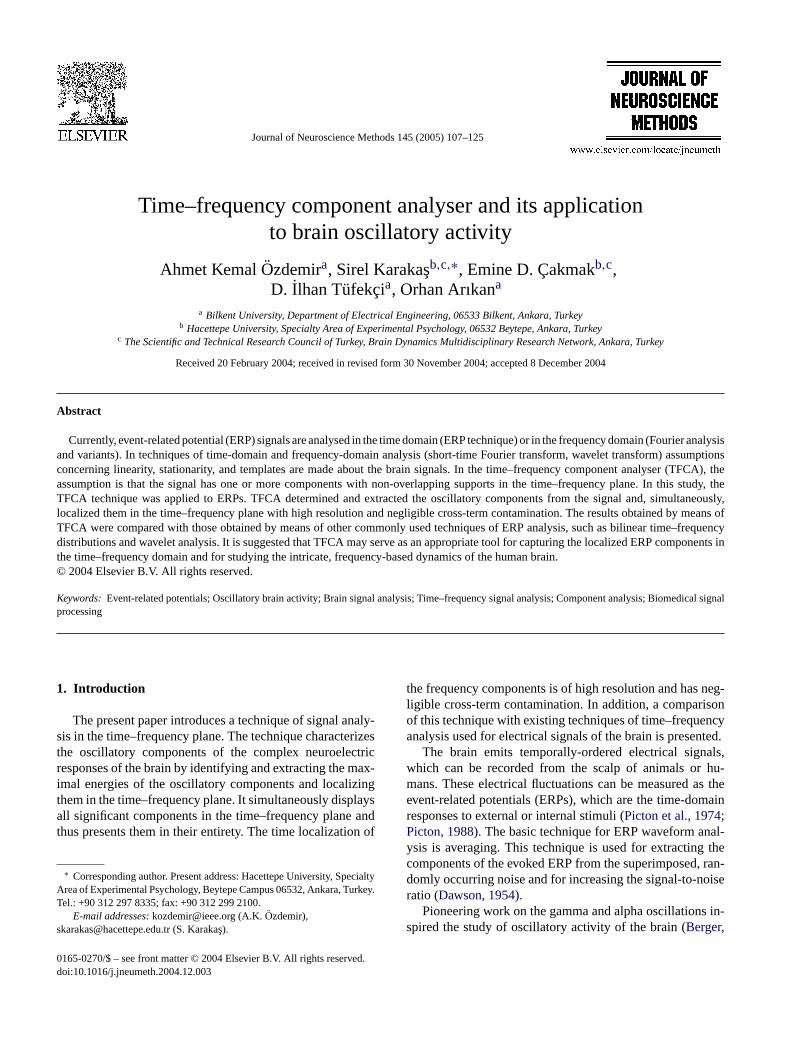
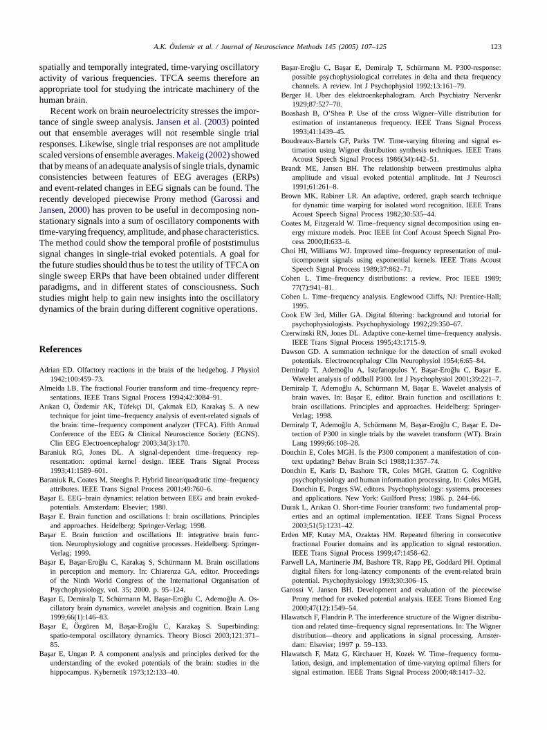
Although the use of Wigner distribution significantly im-proves the resolution of the individual ERP components, theresultant time–frequency description is heavily cluttered bythe cross-terms of the distribution. The cross-terms are oscil-latory artefacts in the time–frequency plane. These artefactsmay interfere with the auto-components and decrease theinterpretability of the Wigner distribution. The cross-termsthat occur due to the interaction of different signal compo-nents (i.e. auto-components) in a multi-component signal arecalledouter interference (cross) terms, and the cross-termsthat occur due to the interaction of a single-signal componentwith itself are calledinner interference (cross) terms (Fig. 1)(Hlawatsch and Flandrin, 1997). Because of the existence ofcross-terms, the Wigner distribution of ERPs cannot providethe desired result.
To overcome cross-term cluttering in the Wignerdistribution-based analysis of ERP, a short-time analysis tech-nique has recently been proposed that applies adaptive filterson the Wigner distribution (Jones and Baraniuk, 1995; Tagluket al., 2002, in press). To emphasize the high frequency fea-tures that have low energy, ERP was decomposed into sixs dis-t sub-b theo encyd sig-n pay-o wert utionb
rge-a themi rk,t ibu-t lass
of time–frequency distributions (Cohen, 1989). In this class,the time–frequency distributions of a signalx(t) are given by
TFx(t, f ) =∫ ∞
−∞
∫ ∞
−∞κ(ν, τ)Ax(ν, τ)e−j2π(νt+τf ) dν dτ,
(2)
where κ(ν, τ) is called the kernel of the transformation(Cohen, 1989, 1995) andAx(ν, τ) is the symmetric ambi-guity function (AF) which is defined as the two-dimensionalinverse Fourier transform (FT) of the Wigner distribution
Ax(ν, τ) �∫ ∞
−∞
∫ ∞
−∞Wx(t, f )ej2π(νt+τf ) dt df
=∫ ∞
−∞x
(t + τ
2
)x∗
(t − τ
2
)ej2πνt dt. (3)
Traditionally, the low-pass smoothing kernelκ(ν, τ) is de-signed to let pass the auto-terms that are centered at the ori-gin of the AF plane, and to suppress the cross-terms that arelocated away from the origin. The properties of the result-ing time–frequency distribution are thus closely related tothose of the chosen kernel (for a review of some of this typeof time–frequency distributions withfixed kernels, seePage,1952; Mergenau and Hill, 1961; Choi and Williams, 1989;Cohen, 1989). Usually, these distributions perform well onlyf AFp ernelκ oodc on.
xedk osed(i rnel(c pass-b st f thea erms fixed
F he das ) Whet upportS is ct stributio cross-t upport cy plaM to the .
ub-bands. Using short time, adaptively filtered Wignerributions, time–frequency analysis was made on eachand. Finally, using a frequency weighting to provideverall time–frequency representation, the time–frequistributions corresponding to each of the six sub-bandals were merged. As in all STFT applications, there is aff between time and frequency localization. The narro
he chosen time interval, the better the temporal resolut the poorer the frequency resolution, and vice versa.
Since cross-terms in the Wigner distribution are lamplitude oscillations, another approach to suppress
s to smooth the Wigner distribution. In a unified framewohe distributions obtained by smoothing the Wigner distrion were studied under the name of Cohen’s bilinear c
ig. 1. Wigner distributions of some artificially generated signals. Time–frequency support of the signal is convex (a time–frequency she connecting line segmentAiAj is also contained inS), the Wigner dierm interference. (b) On the other hand, a non-convex auto-term sulti-component signals lead to outer interference terms that are due
or a limited class of signals whose auto-terms in thelane are located inside the pass-band region of the k(ν, τ). For other signals, they offer a trade-off between gross-term suppression and high auto-term concentrati
To overcome the shortcomings of the TFDs with fiernels, TFDs with signal-dependent kernels were propBaraniuk and Jones, 1993; Czerwinski and Jones, 1995). Fornstance, the well-known optimal radially Gaussian keORGK) design adaptively chooses the kernelκ(ν, τ) toover the auto-terms and to keep cross-terms out of itsand (Baraniuk and Jones, 1993). Signal-dependent TFD
hat adapt the pass-band of the kernel to the location outo-terms in the AF domain usually offer better cross-tuppression and higher resolution than the TFDs with
hed lines outline the support of the respective auto-components. (an thealledconvexif for each pair of its pointsAi = (ti , fi ) andBj = (tj , fj ) in S,n has a very high auto-term concentration, and there is negligibleproduces cross-terms, inner interference terms, in the time–frequenne. (c)interaction between different auto-terms in the time–frequency plane
110 A.K. Ozdemir et al. / Journal of Neuroscience Methods 145 (2005) 107–125
kernels. However, design of a single kernel for the entiresignal may lead to some compromises when analysingmulti-component signals (Jones and Baraniuk, 1995). Theadaptation of the kernel at each time to achieve optimal localperformance usually provides better TFDs at the expense ofsignificantly increased computational complexity (Jones andBaraniuk, 1995). Nevertheless, the design of a single kernelat each time instant may lead to similar compromises asin ORGK when there are signal components that overlapin time.
This paper presents a new technique, TFCA, that pro-vides a high-resolution time–frequency characterization oflocalized signal components (Arıkan et al., 2003;Ozdemirand Arıkan, 2000, 2001;Ozdemir et al., 2001;Ozdemir,2003). The only assumption made about the componentsof the signal is that they have non-overlapping supports inthe time–frequency plane. As explained in Section2.4.2,this assumption on the signal components can be relaxed aswell. Under the assumption of non-overlapping signal com-ponents, the TFCA technique makes use of a componentadaptive time warping operation to transform analysed signalcomponents with non-convex supports into ones with convexsupports. The warped signal components are extracted byusing a time–frequency domain incision algorithm and theircorresponding distributions are computed by using direction-ally smoothed Wigner analysis. The idea is that, for signalsw riort ter-f tion,t ped,c s ex-t nt iss alysisi r allc
ofw RPs byu s ac rt oft mages teds andt tion,t uti-l gle-v ngt ques.H entso hosec ands rota-t
ver-s eent uter
interference terms) and within the component itself (innerinterference terms), while preserving the time–frequencylocalization of the auto-components. As ERPs have localizedtime–frequency supports, the TFCA technique may be anappropriate tool for high-resolution ERP analysis. It mayprovide both an accurate time domain identification and rep-resentation of the frequency components that constitute theERP. TFCA can also extract individual signal componentsfrom noisy recordings.
The aim of the present study has been to describethe TFCA technique, and to test its applicability totime–frequency analysis of ERP signals. The technique wastested on a simulated signal and on ERPs that were obtainedunder the active oddball (OB) paradigm (Sutton et al., 1965).Since the ERP components and also the ERO components thatform the OB waveform have been well established (Basar-Eroglu et al., 1992; Polich and Kok, 1995; Karakas¸ et al.,2000a, 2000b), ERP of OB is an appropriate signal for test-ing the utility of a signal analysis technique, and for demon-strating the advantages that the technique may possess overothers currently used, and cited in the literature. The presentstudy compared the findings that were obtained with TFCAto those obtained with the commonly used time–frequencytechnique, the Wigner analysis.
2
2
ringa werer ectsw osei orp ere,a avea suchm ntials metrict ualsw dy,e
2
iona . Thed itha uli( abil-i ballp enceo hadbe
ith convex supports Wigner distribution provides supeime–frequency resolution with negligible cross-term inerence. Finally, by using an inverse warping transformahe cross-term free distribution of the original, i.e. unwaromponents are obtained. In TFCA, after a component iracted and its distribution is computed, that componeubtracted from the analysed signal and the same ans conducted on the residual signal until distributions foomponents are obtained.
One of the contributions of this paper is introductionarping transformation into time–frequency analysis of Eignals. As detailed, the warping function is computedsing short-time Fourier transformation, which provideoarse but cross-term free distribution. Then, the suppohe analysed signal component is isolated by using an iegmentation algorithm. After the orientation of the isolaupport is identified, time–frequency domain rotationsranslations (enabled by fractional Fourier transformaime shifts and frequency modulations, respectively) areized to obtain a support which has a positive and sinaluedspine. Finally, the warping function correspondio estimated spine is computed by quadrature technience, in TFCA, it is assumed that the signal componf the brain have localized time–frequency supports worresponding spines can be transformed into positiveingle-valued spines by using time–frequency domainions and translations.
In contrast to Wigner distribution and its smoothedions, TFCA yields negligible cross-term cluttering betwhe different components in the composite signal (o
. Methods and materials
.1. Subjects
The data were acquired from 20 young volunteedults (18–29 years; 5 males and 15 females) whoecruited from the university student population. Subjere naive to electrophysiological studies. Only th
ndividuals who reported being free of neurologicalsychiatric problems were accepted. Individuals who wt the time of testing, under medication that would hffected cognitive processes or who stopped takingedication, were excluded. The hearing level of the pote
ubjects was assessed through computerized audioesting prior to the experimental procedures. Individith hearing deficits were not included in the stuither.
.2. Stimuli and paradigms
The auditory stimuli had 10 ms r/f time, 50 ms duratnd were presented over the headphones at 65 dB SPLeviant stimuli (n= 30–33, 2000 Hz) occurred randomly wprobability of about 0.20 within a series of standard stimn= 120–130, 1000 Hz) that were presented with a probty of about 0.80. According to the procedures of the oddaradigm, participants had to mentally count the occurrf deviant stimuli and to report them after the sessioneen terminated (for details of the methodology, seeKarakast al., 2000a).
A.K. Ozdemir et al. / Journal of Neuroscience Methods 145 (2005) 107–125 111
2.3. Electrophysiological procedures
Electrical activity of the brain, the prestimulus elec-troencephalogram (EEG) and the poststimulus ERP, wererecorded in an electrically shielded, sound-proof chamber.Recordings were taken from 15 recording sites (ref: linkedearlobes; ground: forehead) of the 10–20 system undereyes-open condition. The present study reports findingsfrom the Fz recording site.
Bipolar recordings were made of electro-ocular and elec-tromyographic activity for online rejection (of responseswhose amplitudes exceeded±50�V) and offline rejec-tion (through visual inspection) of artefacts. Rejection oc-curred for epochs that contained gross muscular activity,eye-movements or blinks. Electrical activity was amplifiedand filtered with a bandpass between 0.16 and 70 Hz (3 dBdown, 12 dB/octave). It was recorded with a sampling rateof 500 Hz and a total recording time of 2048 ms, 1024 msof which served as the prestimulus baseline. EEG-ERP dataacquisition, analysis, and storage were achieved by a com-mercial system (Brain Data 2.92). A notch filter (50 Hz) wasnot activated.
2.4. Description of TFCA: procedures and applications
tion2 rp-ia on-s FCAi encya
2s
ss-i dR rald,2 thef dϕ
f hase,ζ nt.W ingf atf o-r e uti-l
ne-p orm.T -f
x
where the kernel of the transformationBa(t, t′) is
Ba(t, t′) = Aφ exp(jπ(t2 cotφ − 2tt′ cscφ + t′2 cotφ)),
Aφ = exp(−jπ sgn(sinφ)/4 + jφ/2)
| sinφ|1/2, φ = a
π
2. (5)
From this definition, it follows that first-order FrFT is the or-dinary Fourier transform and zeroth-order FrFT is the func-tion itself. The definition of the FrFT is easily extended tooutside the interval [−2, 2] by noting thatF4k is the identityoperator for any integerk and FrFT is additive in index, i.e.{Fa1{Fa2x}}(t) = {Fa1+a2x}(t).
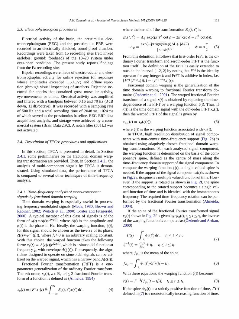
Fractional domain warping is the generalization of thetime domain warping to fractional Fourier transform do-mains (Ozdemir et al., 2001). The warped fractional Fouriertransform of a signalx(t) is obtained by replacing the time-dependence of its FrFT by a warping functionζ(t). Thus, ifx(t) is the time domain signal with theath-order FrFTxa(t),then the warped FrFT of the signal is given by
xa,ζ(t) = xa(ζ(t)), (6)
whereζ(t) is the warping function associated withxa(t).In TFCA, high resolution distribution of signal compo-
nents with non-convex time–frequency support (Fig. 2b) isobtained using adaptively chosen fractional domain warp-ing transformations. For each analysed signal component,t om-p g thet t. Toc isni w-ec val-u ousf per-f1
nalxo ,2
w
f
W
ζ
Id e.
In this section, TFCA is presented in detail. In Sec.4.1, some preliminaries on the fractional domain wa
ng transformation are provided. Then, in Section2.4.2., thenalysis of multi-component signals by TFCA is demtrated. Using simulated data, the performance of Ts compared to several other techniques of time–frequnalysis.
.4.1. Time–frequency analysis of mono-componentignals by fractional domain warping
Time domain warping is especially useful in proceng frequency-modulated signals (Meda, 1980; Brown anabiner, 1982; Wulich et al., 1990; Coates and Fitzge000). A typical member of this class of signals is of
orm of x(t) =A(t)ej2πϕ(t), whereA(t) is the amplitude an(t) is the phase in Hz. Ideally, the warping function,ζ(t),
or this signal should be chosen as the inverse of its p(t) =ϕ−1(fst), wherefs > 0 is an arbitrary scaling constaith this choice, the warped function takes the follow
orm:xζ(t) = A(ζ(t))ej2πfst , which is a sinusoidal functionrequencyfs with envelopeA(ζ(t)). Consequently, the algithms designed to operate on sinusoidal signals can bized on the warped signal, which has a narrow bandA(ζ(t)).
Fractional Fourier transformation (FrFT) is a oarameter generalization of the ordinary Fourier transfheath-order,xa(t), a∈ R, |a| ≤ 2 fractional Fourier trans
orm of a function is defined as (Almeida, 1994)
a(t) = {Fax}(t)�∫ ∞
−∞Ba(t, t
′)x(t′) dt′, (4)
he warping function is determined on the basis of the conent’s spine, defined as the centre of mass alon
ime–frequency domain support of the signal componenompute the warping functionζ(t), a single-valued spineeeded. If the support of the signal componentx(t) is as shown
n Fig. 2e, its spine is a multiple valued function of time. Hover, if the support is rotated as shown inFig. 2f, the spineorresponding to the rotated support becomes a singleed function of time and is identical with the instantane
requency. The required time–frequency rotation can beormed by the fractional Fourier transformation (Almeida,994).
If the spine of the fractional Fourier transformed siga(t) shown inFig. 2f is given byψa(t), ti ≤ t≤ tf , the inversef the warping function is computed as (Ozdemir and Arıkan000)
Γ (t) =∫ t
ti
ψa(t′) dt′, ti ≤ t ≤ tf,
ζ−1(t) = Γ (t)fψa
+ ti, ti ≤ t ≤ tf,
(7)
herefψa is the mean of the spine
ψa =∫ tf
ti
ψa(t′) dt′/(tf − ti ). (8)
ith these equations, the warping functionζ(t) becomes
(t) = Γ−1(fψa (t − ti )), ti ≤ t ≤ tf . (9)
f the spineψa(t) is a strictly positive function of time,Γ (t)efined in(7) is a monotonically increasing function of tim
112 A.K. Ozdemir et al. / Journal of Neuroscience Methods 145 (2005) 107–125
Fig. 2. (a) A signalx(t) and (b) its (−0.75)th-order FrFTx(−0.75)(t); (c) the Wigner distributions ofx(t) and (d)x(−0.75)(t); (e) the spines ofx(t) and (f)x(−0.75)(t)plotted on the support of their auto-term Wigner distributions. Although the spine in (e) is a multi-valued function of time, the spine correspondingto the rotatedsupport becomes a single-valued function of time as shown in (f).
Therefore, its inverse given in(9) exists and it is unique. Oth-erwise, the frequency-modulated signalx
δfa (t)� xa(t)ej2πtδf is
used, whereδf is chosen such that the spineψδfa (t)�ψa(t) +
δf of xδfa (t) is a strictly positive function of time. Hence, for
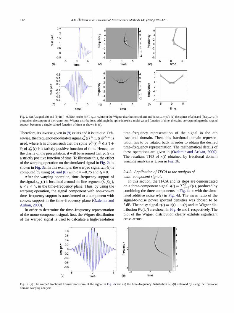
the clarity of the presentation, it will be assumed thatψa(t) isa strictly positive function of time. To illustrate this, the effectof the warping operation on the simulated signal inFig. 2a isshown inFig. 3a. In this example, the warped signalxa,ζ(t) iscomputed by using(4) and (6)with a=−0.75 andδf = 0.
After the warping operation, time–frequency support ofthe signalxa,ζ(t) is localized around the line segment (t, fψa ),ti ≤ t ≤ tf , in the time–frequency plane. Thus, by using thewarping operation, the signal component with non-convextime–frequency support is transformed to a component withconvex support in the time–frequency plane (Ozdemir andArıkan, 2000).
In order to determine the time–frequency representationof the mono-component signal, first, the Wigner distributionof the warped signal is used to calculate a high-resolution
time–frequency representation of the signal in theathfractional domain. Then, this fractional domain represen-tation has to be rotated back in order to obtain the desiredtime–frequency representation. The mathematical details ofthese operations are given in (Ozdemir and Arıkan, 2000).The resultant TFD ofx(t) obtained by fractional domainwarping analysis is given inFig. 3b.
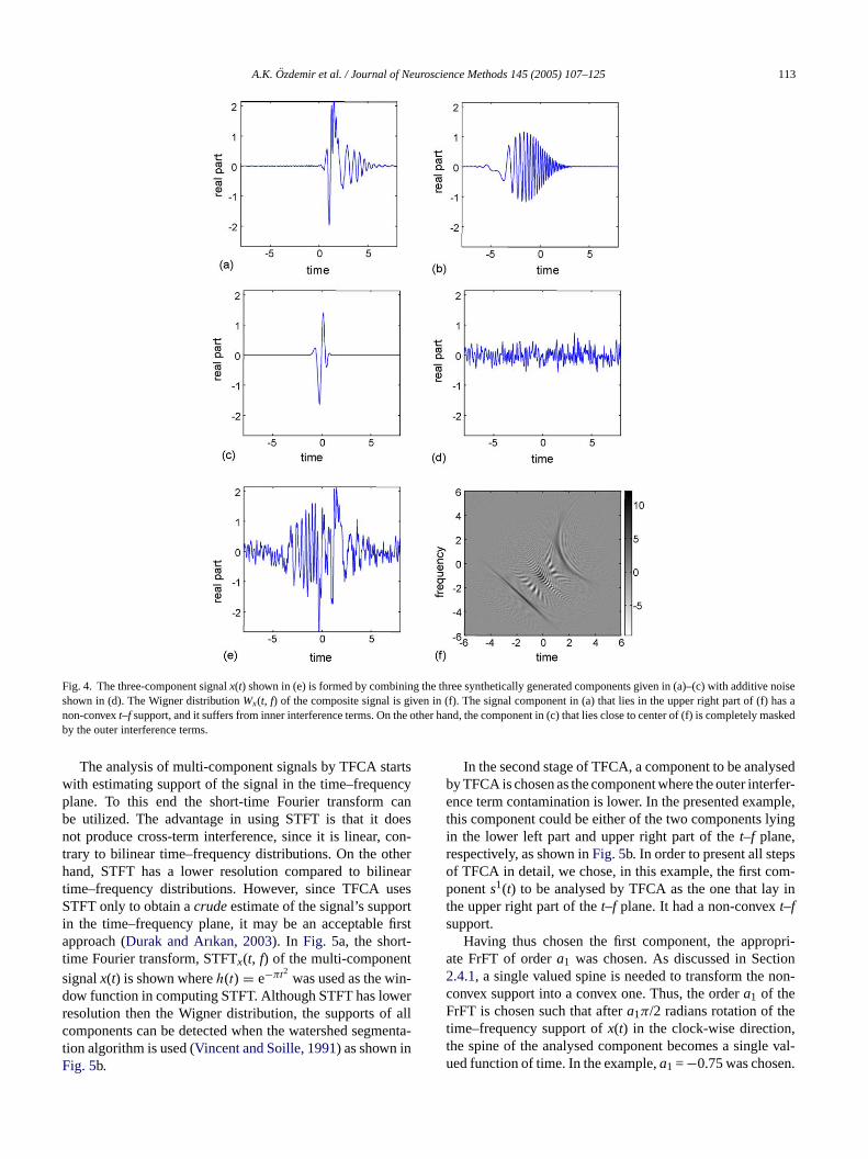
2.4.2. Application of TFCA to the analysis ofmulti-component signals
In this section, the TFCA and its steps are demonstratedon a three-component signals(t) = ∑3
i=1si(t), produced by
combining the three components inFig. 4a–c with the simu-lated additive noisew(t) in Fig. 4d. The mean ratio of thesignal-to-noise power spectral densities was chosen to be5 dB. The noisy signalx(t) = s(t) + w(t) and its Wigner dis-tributionWx(t, f) are shown inFig. 4e and f, respectively. Theplot of the Wigner distribution clearly exhibits significantcross-terms.
F a and ( ald
ig. 3. (a) The warped fractional Fourier transform of the signal inFig. 2omain warping analysis.
b) the time–frequency distribution ofx(t) obtained by using the fraction
A.K. Ozdemir et al. / Journal of Neuroscience Methods 145 (2005) 107–125 113
Fig. 4. The three-component signalx(t) shown in (e) is formed by combining the three synthetically generated components given in (a)–(c) with additive noiseshown in (d). The Wigner distributionWx(t, f) of the composite signal is given in (f). The signal component in (a) that lies in the upper right part of (f) has anon-convext–f support, and it suffers from inner interference terms. On the other hand, the component in (c) that lies close to center of (f) is completely maskedby the outer interference terms.
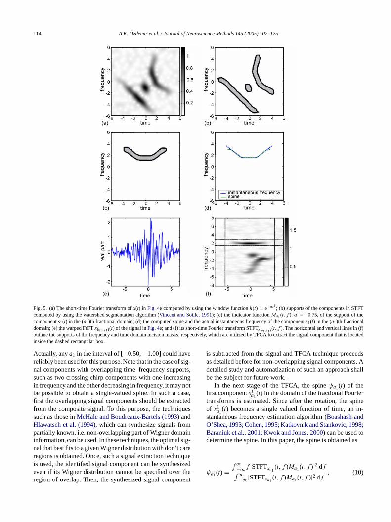
The analysis of multi-component signals by TFCA startswith estimating support of the signal in the time–frequencyplane. To this end the short-time Fourier transform canbe utilized. The advantage in using STFT is that it doesnot produce cross-term interference, since it is linear, con-trary to bilinear time–frequency distributions. On the otherhand, STFT has a lower resolution compared to bilineartime–frequency distributions. However, since TFCA usesSTFT only to obtain acrudeestimate of the signal’s supportin the time–frequency plane, it may be an acceptable firstapproach (Durak and Arıkan, 2003). In Fig. 5a, the short-time Fourier transform, STFTx(t, f) of the multi-componentsignalx(t) is shown whereh(t) = e−πt2 was used as the win-dow function in computing STFT. Although STFT has lowerresolution then the Wigner distribution, the supports of allcomponents can be detected when the watershed segmenta-tion algorithm is used (Vincent and Soille, 1991) as shown inFig. 5b.
In the second stage of TFCA, a component to be analysedby TFCA is chosen as the component where the outer interfer-ence term contamination is lower. In the presented example,this component could be either of the two components lyingin the lower left part and upper right part of thet–f plane,respectively, as shown inFig. 5b. In order to present all stepsof TFCA in detail, we chose, in this example, the first com-ponents1(t) to be analysed by TFCA as the one that lay inthe upper right part of thet–f plane. It had a non-convext–fsupport.
Having thus chosen the first component, the appropri-ate FrFT of ordera1 was chosen. As discussed in Section2.4.1, a single valued spine is needed to transform the non-convex support into a convex one. Thus, the ordera1 of theFrFT is chosen such that aftera1π/2 radians rotation of thetime–frequency support ofx(t) in the clock-wise direction,the spine of the analysed component becomes a single val-ued function of time. In the example,a1 =−0.75 was chosen.
114 A.K. Ozdemir et al. / Journal of Neuroscience Methods 145 (2005) 107–125
Fig. 5. (a) The short-time Fourier transform ofx(t) in Fig. 4e computed by using the window functionh(t) = e−πt2; (b) supports of the components in STFTcomputed by using the watershed segmentation algorithm (Vincent and Soille, 1991); (c) the indicator functionMa1(t, f ), a1 =−0.75, of the support of thecomponents1(t) in the (a1)th fractional domain; (d) the computed spine and the actual instantaneous frequency of the components1(t) in the (a1)th fractionaldomain; (e) the warped FrFTx(a1,ς1)(t) of the signal inFig. 4e; and (f) its short-time Fourier transform STFTx(a1,ς1) (t, f ). The horizontal and vertical lines in (f)outline the supports of the frequency and time domain incision masks, respectively, which are utilized by TFCA to extract the signal component that islocatedinside the dashed rectangular box.
Actually, anya1 in the interval of [−0.50,−1.00] could havereliably been used for this purpose. Note that in the case of sig-nal components with overlapping time–frequency supports,such as two crossing chirp components with one increasingin frequency and the other decreasing in frequency, it may notbe possible to obtain a single-valued spine. In such a case,first the overlapping signal components should be extractedfrom the composite signal. To this purpose, the techniquessuch as those inMcHale and Boudreaux-Bartels (1993)andHlawatsch et al. (1994), which can synthesize signals frompartially known, i.e. non-overlapping part of Wigner domaininformation, can be used. In these techniques, the optimal sig-nal that best fits to a given Wigner distribution with don’t careregions is obtained. Once, such a signal extraction techniqueis used, the identified signal component can be synthesizedeven if its Wigner distribution cannot be specified over theregion of overlap. Then, the synthesized signal component
is subtracted from the signal and TFCA technique proceedsas detailed before for non-overlapping signal components. Adetailed study and automatization of such an approach shallbe the subject for future work.
In the next stage of the TFCA, the spineψa1(t) of thefirst components1
a1(t) in the domain of the fractional Fourier
transforms is estimated. Since after the rotation, the spineof s1
a1(t) becomes a single valued function of time, an in-
stantaneous frequency estimation algorithm (Boashash andO’Shea, 1993; Cohen, 1995; Katkovnik and Stankovic, 1998;Baraniuk et al., 2001; Kwok and Jones, 2000) can be used todetermine the spine. In this paper, the spine is obtained as
ψa1(t) =∫ ∞
−∞f |STFTxa1(t, f )Ma1(t, f )|2 df∫ ∞
−∞|STFTxa1(t, f )Ma1(t, f )|2 df
, (10)
A.K. Ozdemir et al. / Journal of Neuroscience Methods 145 (2005) 107–125 115
where the magnitude squared STFT is called spectrogram,which is a smoothed bilineart–f distribution (Cohen, 1995)and the maskMa1(t, f ) is the indicator function of the supportof s1
a1(t), which was obtained automatically using watershed
segmentation algorithm (Vincent and Soille, 1991). In thepresented example, the estimate of the spineψa1(t), computedby using the indicator functionMa1(t, f ) in Fig. 5c, was ob-tained as shown inFig. 5d. In this example, the correspondingroot mean square estimation error for the spine was 0.102 Hz.Then, the warped FrFT inx(a1,ζ1)(t) Fig. 5e was computed.In order to determine the support of the first warped compo-nent, the short-time Fourier transform STTFx(a1,ζ1)(t, f ) ofthe warped signal, was calculated (Fig. 5f). The STFT com-ponent with convex support corresponds to the first warpedcomponent. Note that in the computation of the STFT, a Gaus-sian window,h(t) = e−πt2/4, was used.
The next stage of processing involved the extraction ofthe warped signal component. For this purpose, varioustime–frequency processing techniques (e.g.Hlawatsch et al.,1994, 2000; Erden et al., 1999; Hlawatsch and Kozek, 1994;McHale and Boudreaux-Bartels, 1993; Boudreaux-Bartelsand Parks, 1986) can be used. In the following, results basedon the time–frequency domain incision technique (Erdenet al., 1999) will be presented. The warped signal compo-nent could be extracted by using a simple incision tech-nS efi andt gnalc wa-t f them e firsc nbt sig-n d thisc waso
s
wF* anec uriert
s
Ir n inFT indi-c isiona
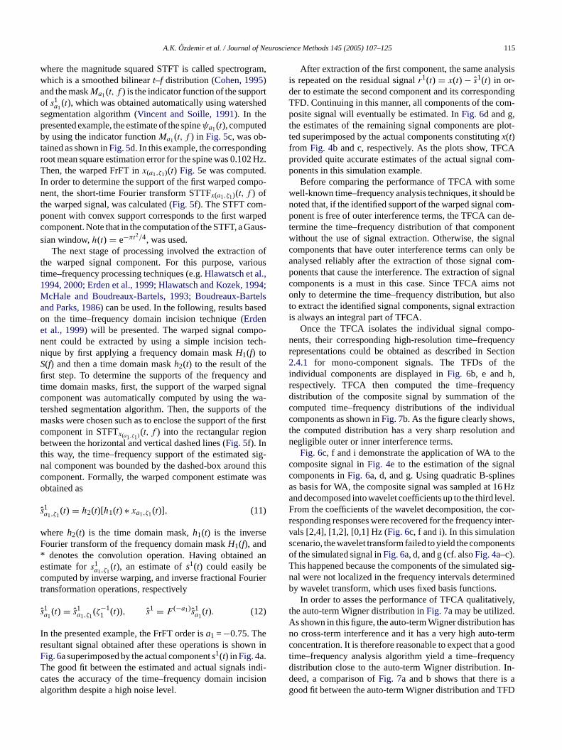
After extraction of the first component, the same analysisis repeated on the residual signalr1(t) = x(t) − s1(t) in or-der to estimate the second component and its correspondingTFD. Continuing in this manner, all components of the com-posite signal will eventually be estimated. InFig. 6d and g,the estimates of the remaining signal components are plot-ted superimposed by the actual components constitutingx(t)from Fig. 4b and c, respectively. As the plots show, TFCAprovided quite accurate estimates of the actual signal com-ponents in this simulation example.
Before comparing the performance of TFCA with somewell-known time–frequency analysis techniques, it should benoted that, if the identified support of the warped signal com-ponent is free of outer interference terms, the TFCA can de-termine the time–frequency distribution of that componentwithout the use of signal extraction. Otherwise, the signalcomponents that have outer interference terms can only beanalysed reliably after the extraction of those signal com-ponents that cause the interference. The extraction of signalcomponents is a must in this case. Since TFCA aims notonly to determine the time–frequency distribution, but alsoto extract the identified signal components, signal extractionis always an integral part of TFCA.
Once the TFCA isolates the individual signal compo-nents, their corresponding high-resolution time–frequencyrepresentations could be obtained as described in Section2 thei ,r ncyd thec ualc s,t andn
thec alc esa 6 Hza evel.F cor-r inter-v ns entsoT d sig-n inedb
ely,t .A hasn termc goodt ncyd In-d ag FD
ique by first applying a frequency domain maskH1(f) to(f) and then a time domain maskh2(t) to the result of thrst step. To determine the supports of the frequencyime domain masks, first, the support of the warped siomponent was automatically computed by using theershed segmentation algorithm. Then, the supports oasks were chosen such as to enclose the support of th
omponent in STFTx(a1,ζ1) (t, f ) into the rectangular regioetween the horizontal and vertical dashed lines (Fig. 5f). In
his way, the time–frequency support of the estimatedal component was bounded by the dashed-box arounomponent. Formally, the warped component estimatebtained as
1a1,ζ1
(t) = h2(t)[h1(t) ∗ xa1,ζ1(t)], (11)
hereh2(t) is the time domain mask,h1(t) is the inverseourier transform of the frequency domain maskH1(f), anddenotes the convolution operation. Having obtained
stimate fors1a1,ζ1
(t), an estimate ofs1(t) could easily beomputed by inverse warping, and inverse fractional Foransformation operations, respectively
1a1
(t) = s1a1,ζ1
(ζ−11 (t)), s1 = F (−a1)s1
a1(t). (12)
n the presented example, the FrFT order isa1 =−0.75. Theesultant signal obtained after these operations is showig. 6a superimposed by the actual components1(t) in Fig. 4a.he good fit between the estimated and actual signalsates the accuracy of the time–frequency domain inclgorithm despite a high noise level.
t
.4.1 for mono-component signals. The TFDs ofndividual components are displayed inFig. 6b, e and hespectively. TFCA then computed the time–frequeistribution of the composite signal by summation ofomputed time–frequency distributions of the individomponents as shown inFig. 7b. As the figure clearly showhe computed distribution has a very sharp resolutionegligible outer or inner interference terms.
Fig. 6c, f and i demonstrate the application of WA toomposite signal inFig. 4e to the estimation of the signomponents inFig. 6a, d, and g. Using quadratic B-splins basis for WA, the composite signal was sampled at 1nd decomposed into wavelet coefficients up to the third lrom the coefficients of the wavelet decomposition, theesponding responses were recovered for the frequencyals [2,4], [1,2], [0,1] Hz (Fig. 6c, f and i). In this simulatiocenario, the wavelet transform failed to yield the componf the simulated signal inFig. 6a, d, and g (cf. alsoFig. 4a–c).his happened because the components of the simulateal were not localized in the frequency intervals determy wavelet transform, which uses fixed basis functions.
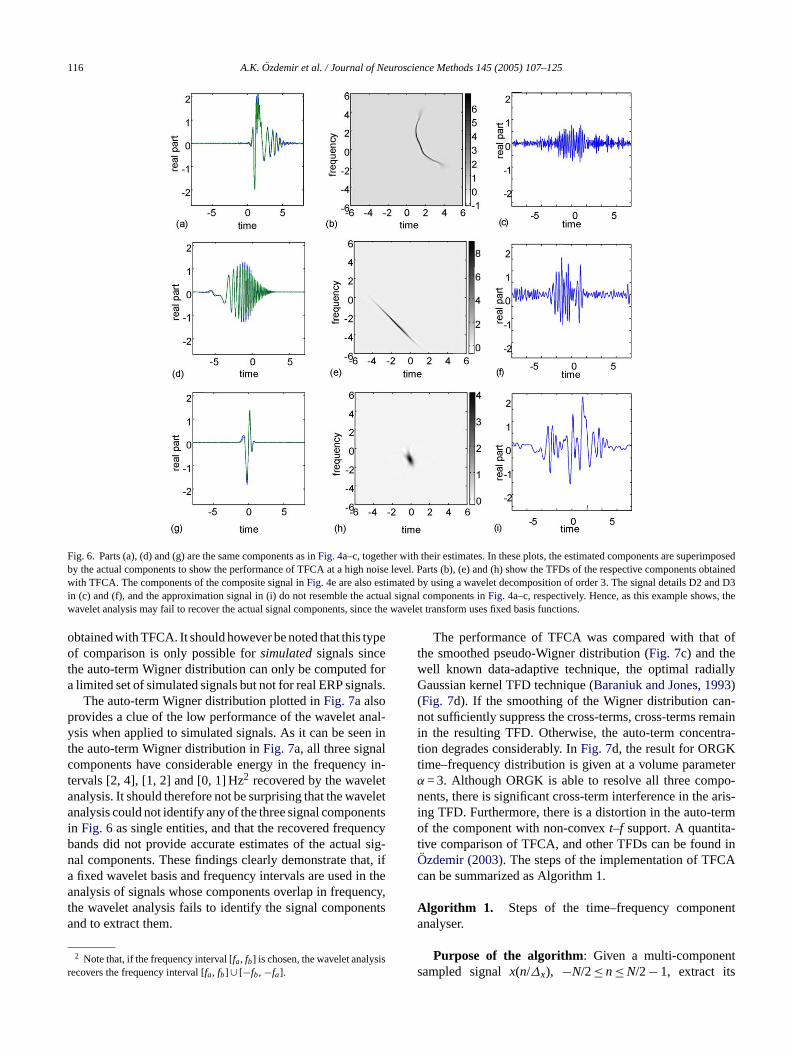
In order to asses the performance of TFCA qualitativhe auto-term Wigner distribution inFig. 7a may be utilizeds shown in this figure, the auto-term Wigner distributiono cross-term interference and it has a very high auto-oncentration. It is therefore reasonable to expect that aime–frequency analysis algorithm yield a time–frequeistribution close to the auto-term Wigner distribution.eed, a comparison ofFig. 7a and b shows that there isood fit between the auto-term Wigner distribution and T
116 A.K. Ozdemir et al. / Journal of Neuroscience Methods 145 (2005) 107–125
Fig. 6. Parts (a), (d) and (g) are the same components as inFig. 4a–c, together with their estimates. In these plots, the estimated components are superimposedby the actual components to show the performance of TFCA at a high noise level. Parts (b), (e) and (h) show the TFDs of the respective components obtainedwith TFCA. The components of the composite signal inFig. 4e are also estimated by using a wavelet decomposition of order 3. The signal details D2 and D3in (c) and (f), and the approximation signal in (i) do not resemble the actual signal components inFig. 4a–c, respectively. Hence, as this example shows, thewavelet analysis may fail to recover the actual signal components, since the wavelet transform uses fixed basis functions.
obtained with TFCA. It should however be noted that this typeof comparison is only possible forsimulatedsignals sincethe auto-term Wigner distribution can only be computed fora limited set of simulated signals but not for real ERP signals.
The auto-term Wigner distribution plotted inFig. 7a alsoprovides a clue of the low performance of the wavelet anal-ysis when applied to simulated signals. As it can be seen inthe auto-term Wigner distribution inFig. 7a, all three signalcomponents have considerable energy in the frequency in-tervals [2, 4], [1, 2] and [0, 1] Hz2 recovered by the waveletanalysis. It should therefore not be surprising that the waveletanalysis could not identify any of the three signal componentsin Fig. 6as single entities, and that the recovered frequencybands did not provide accurate estimates of the actual sig-nal components. These findings clearly demonstrate that, ifa fixed wavelet basis and frequency intervals are used in theanalysis of signals whose components overlap in frequency,the wavelet analysis fails to identify the signal componentsand to extract them.
2 Note that, if the frequency interval [fa, fb] is chosen, the wavelet analysisrecovers the frequency interval [fa, fb] ∪ [−fb, −fa].
The performance of TFCA was compared with that ofthe smoothed pseudo-Wigner distribution (Fig. 7c) and thewell known data-adaptive technique, the optimal radiallyGaussian kernel TFD technique (Baraniuk and Jones, 1993)(Fig. 7d). If the smoothing of the Wigner distribution can-not sufficiently suppress the cross-terms, cross-terms remainin the resulting TFD. Otherwise, the auto-term concentra-tion degrades considerably. InFig. 7d, the result for ORGKtime–frequency distribution is given at a volume parameterα= 3. Although ORGK is able to resolve all three compo-nents, there is significant cross-term interference in the aris-ing TFD. Furthermore, there is a distortion in the auto-termof the component with non-convext–f support. A quantita-tive comparison of TFCA, and other TFDs can be found inOzdemir (2003). The steps of the implementation of TFCAcan be summarized as Algorithm 1.
Algorithm 1. Steps of the time–frequency componentanalyser.
Purpose of the algorithm: Given a multi-componentsampled signalx(n/∆x), −N/2≤n≤N/2− 1, extract its
A.K. Ozdemir et al. / Journal of Neuroscience Methods 145 (2005) 107–125 117
Fig. 7. (a) Auto-term Wigner distribution of the simulated signal inFig. 4e which was obtained by removing the interference terms from the Wignerdistribution in Fig. 4f. Note that, although the auto-term Wigner distribution is a desired distribution, it is, in practice, not computable. It couldhave been computed in this simulation example, because the simulated components, which constitute the multi-component signal, were available. Parts(b)–(d) show the time–frequency distributions obtained with TFCA, the smoothed pseudo-Wigner distribution and the optimal radially Gaussian kerneltime–frequency distribution, respectively. In this example, the volume parameter of ORGK was chosenα= 3, and respective lengths of the time and fre-quency smoothing windows for the smoothed pseudo-Wigner distribution were chosenN/10 andN/4, whereN was the duration of the sampled analysedsignal.
components and compute its time–frequency distribution. Itis assumed thatx(t) is scaled before its sampling so that itsWigner distribution is inside a circle of a diameter∆x ≤ √
N
(seeOzaktas et al., 1996).
Steps of the algorithm:
1. Initialize the residual signal and the iteration number asr0(t) := x(t), i := 1, respectively.
2. Identify the time–frequency support of the compo-nent si(t) using the watershed segmentation algorithm(Vincent and Soille, 1991). After manually determiningthe appropriate rotation angleφi and the fractional do-mainai = 2φi /π, estimate the spineψi,ai (t) of the frac-tional Fourier transformxai (t) using an instantaneousfrequency estimation algorithm. Then, determine theamount of the required frequency shiftδfi on the spineψi,ai (t).
3. Compute the sampled FrFTri−1ai
(kT ), ai = 2φi /π, fromri−1(kT) using the fast fractional Fourier transform algo-rithm (seeOzaktas et al., 1996).
4. Define the warping functionζi(t) = Γ−1i (fψi (t −
t1)), where Γi(t) = ∫ t
t1[ψai (t
′) + δfi ] dt′ and fψi =Γi(tN )/(tN − t1). Compute the sampled warping func-tion ζi (kT).
5. Compute the sampled warped signalri−1ai,ζi
(kT ) as
ri−1,δfiai (kT ) = ej2πδfi kT ri−1
ai(kT ),
ri−1,δfiai,ζi
(kT ) = e−j2πδfi kT ri−1,δfiai (ζi(kT )).
6. Estimate the ith component by incision of thetime–frequency domain as
si,δfiai,ζi
(t) = h2(t)[h1(t) ∗ ri−1,δfiai,ζi
(t)],
whereh2(t) is a time–domain mask andh1(t) is the in-verse Fourier transform of a frequency domain maskH1(f).
7. For each TFD slice ofsi(t), compute yai,ςi (kT ) =si,δfiai,ζi
(kT )ej2π∆ψζi(kT ), after choosing the slice offset∆ψ.8. Compute the sampled TFDTFyai,ςi
(mT , fψi ), t1/T ≤m ≤ tN/T of yai,ζi (t) using the directional smoothingalgorithm (cf.Ozdemir and Arıkan, 2000), whereT isthe sampling interval of the TFD slice.
9. The TFD slice ofsi(t) is given by
TFsi (tr(mT ), fr(mT )) = TFya,ζ(mT , fψ),
where (tr(mT ), fr(mT )) define a curve in thetime–frequency plane parameterized by the variablemT
118 A.K. Ozdemir et al. / Journal of Neuroscience Methods 145 (2005) 107–125
tr(mT ) = ζ(mT ) cos(aiπ
2
)− (ψ(ζ(mT ))
+∆ψ) sin(aiπ
2
),
fr(mT ) = ζ(mT ) sin(aiπ
2
)+ (ψ(ζ(mT ))
+∆ψ) cos(aiπ
2
),
t1
T≤ m ≤ tN
T.
10. Estimate the sampledsi(t) by taking the inverse ofthe warping, frequency modulation and the fractional
Fourier transformation on the sampledsδfai,ζi
(t)
si,δfia (kT ) = ej2πδfi ζ
−1i (kT )s
i,δfiai,ζi
(ζ−1i (kT )),
siai (kT ) = e−j2πδfi kT si,δfiai (kT ),
si(kT ) = {F (−ai)siai}(kT ).
11. Compute the residual signalri(kT ) = ri−1(kT ) −si(kT ).
if any signal component is left in residual signalri(kT) then
Seti = i + 1, andGOTO step 2,else
Compute thet–f distribution of the compositesignal as the sum of thet–f distributions of in-dividual signal components.
endif
3. Results
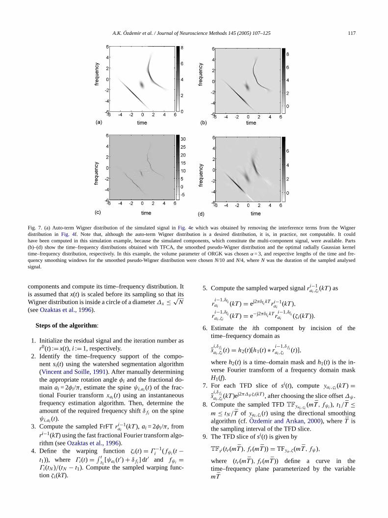
Fig. 8 shows the results of the TFCA analysis of the av-eraged ERP (Fig. 8a) of a trial subject (“GUOZ”). The ERPwas obtained in response to deviant stimuli under the oddballparadigm. The ORGK provided a highly blurred distributionof the ERP components in the time–frequency plane (Fig. 8b).TFCA showed that the ERP was composed of one prestimulus(component 1) and four poststimulus (components 2–5) sig-nal components (Fig. 8c, e, g, i and k) and these were clearlyand sharply localized in the time–frequency plane (Fig. 8d, f,h, j and l). The high amplitude components 2 and 3 along withcomponent 4 contributed to the P300 component of the time
FfE(s
ig. 8. TFCA analysis of the average ERP evoked by deviant stimuli underequency in Hz. Note that the individual time–frequency representations havRP; (b) its ORGK TFD; (c, e, g, i and k) time domain representations of ER
1–5) in the time–frequency distributions; (m) absolute value of the differencuperposition of the extracted time–frequency representations.
r the OB paradigm in a trial subject (“GUOZ”). Right axes (b, d, f, h, j and l):e scales proportional to the strength of the corresponding component.(a) OriginalP components obtained with TFCA; (d, f, h, j and l) corresponding componentse between the reconstructed superposition and the original ERP givenin (a); (n)
A.K. Ozdemir et al. / Journal of Neuroscience Methods 145 (2005) 107–125 119
domain. Component 3 also formed the general waveform ofthe early negative complex in the ERP waveform. Taking thecentral value into account, components 2 and 3 were basicallydue to the delta frequency. However, there were transitionsto neighboring frequencies such that components 2 and 3also included the theta frequency. Component 4 contributedto N100 and N200 in the ERP waveform. Concerning thefrequency, component 4 covered basically the theta but alsothe alpha frequencies. Component 5 was the smallest bothin amplitude and energy and it was due to the beta oscilla-tion. It contributed to the early N100 and N200 peaks on theERP waveform. The mean amplitude of the residual whichwas obtained by subtracting the reconstructed ERP from therecorded ERP was of the order of 0.6�V (Fig. 8m). This in-dicated that composite TFCA (Fig. 8n) yielded an accuratedecomposition of the ERP.
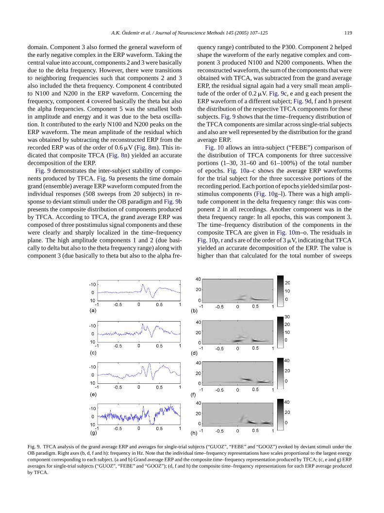
Fig. 9 demonstrates the inter-subject stability of compo-nents produced by TFCA.Fig. 9a presents the time domaingrand (ensemble) average ERP waveform computed from theindividual responses (508 sweeps from 20 subjects) in re-sponse to deviant stimuli under the OB paradigm andFig. 9bpresents the composite distribution of components producedby TFCA. According to TFCA, the grand average ERP wascomposed of three poststimulus signal components and thesewere clearly and sharply localized in the time–frequencyplane. The high amplitude components 1 and 2 (due basi-c withc fre-
quency range) contributed to the P300. Component 2 helpedshape the waveform of the early negative complex and com-ponent 3 produced N100 and N200 components. When thereconstructed waveform, the sum of the components that wereobtained with TFCA, was subtracted from the grand averageERP, the residual signal again had a very small mean ampli-tude of the order of 0.2�V. Fig. 9c, e and g each present theERP waveform of a different subject;Fig. 9d, f and h presentthe distribution of the respective TFCA components for thesesubjects.Fig. 9shows that the time–frequency distribution ofthe TFCA components are similar across single-trial subjectsand also are well represented by the distribution for the grandaverage ERP.
Fig. 10allows an intra-subject (“FEBE”) comparison ofthe distribution of TFCA components for three successiveportions (1–30, 31–60 and 61–100%) of the total numberof epochs.Fig. 10a–c shows the average ERP waveformsfor the trial subject for the three successive portions of therecording period. Each portion of epochs yielded similar post-stimulus components (Fig. 10g–l). There was a high ampli-tude component in the delta frequency range: this was com-ponent 2 in all recordings. Another component was in thetheta frequency range: In all epochs, this was component 3.The time–frequency distribution of the components in thecomposite TFCA are given inFig. 10m–o. The residuals inFig. 10p, r and s are of the order of 3�V, indicating that TFCAy ue ish eps
F gle-tria under theO individ rgycab
ally to delta but also to the theta frequency range) alongomponent 3 (due basically to theta but also to the alpha
ig. 9. TFCA analysis of the grand average ERP and averages for sinB paradigm. Right axes (b, d, f and h): frequency in Hz. Note that the
omponent corresponding to each subject. (a and b) Grand average ERP andverages for single-trial subjects (“GUOZ”, “FEBE” and “GOOZ”); (d, f and h)y TFCA.
ielded an accurate decomposition of the ERP. The valigher than that calculated for the total number of swe
l subjects (“GUOZ”, “FEBE” and “GOOZ”) evoked by deviant stimuliual time–frequency representations have scales proportional to the laest energ
the composite time–frequency representation produced by TFCA; (c, e and g) ERPthe composite time–frequency representations for each ERP average produced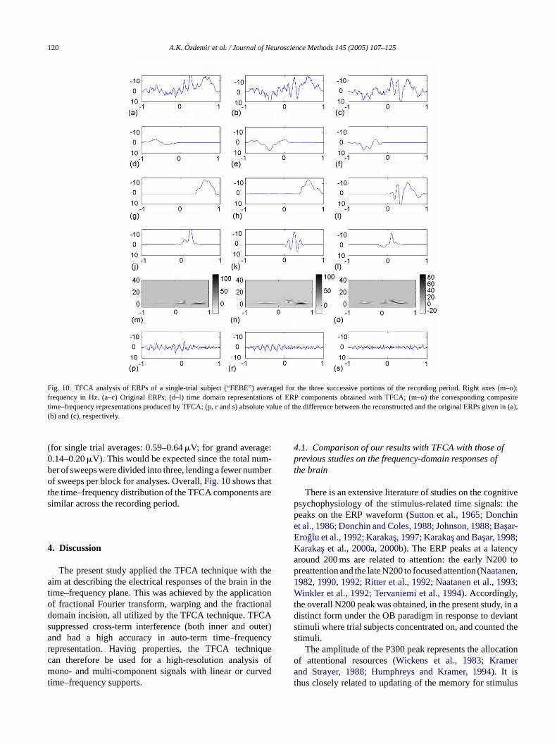
120 A.K. Ozdemir et al. / Journal of Neuroscience Methods 145 (2005) 107–125
Fig. 10. TFCA analysis of ERPs of a single-trial subject (“FEBE”) averaged for the three successive portions of the recording period. Right axes (m–o):frequency in Hz. (a–c) Original ERPs; (d–l) time domain representations of ERP components obtained with TFCA; (m–o) the corresponding compositetime–frequency representations produced by TFCA; (p, r and s) absolute value of the difference between the reconstructed and the original ERPs givenin (a),(b) and (c), respectively.
(for single trial averages: 0.59–0.64�V; for grand average:0.14–0.20�V). This would be expected since the total num-ber of sweeps were divided into three, lending a fewer numberof sweeps per block for analyses. Overall,Fig. 10shows thatthe time–frequency distribution of the TFCA components aresimilar across the recording period.
4. Discussion
The present study applied the TFCA technique with theaim at describing the electrical responses of the brain in thetime–frequency plane. This was achieved by the applicationof fractional Fourier transform, warping and the fractionaldomain incision, all utilized by the TFCA technique. TFCAsuppressed cross-term interference (both inner and outer)and had a high accuracy in auto-term time–frequencyrepresentation. Having properties, the TFCA techniquecan therefore be used for a high-resolution analysis ofmono- and multi-component signals with linear or curvedtime–frequency supports.
4.1. Comparison of our results with TFCA with those ofprevious studies on the frequency-domain responses ofthe brain
There is an extensive literature of studies on the cognitivepsychophysiology of the stimulus-related time signals: thepeaks on the ERP waveform (Sutton et al., 1965; Donchinet al., 1986; Donchin and Coles, 1988; Johnson, 1988; Bas¸ar-Eroglu et al., 1992; Karakas¸, 1997; Karakas¸ and Bas¸ar, 1998;Karakaset al., 2000a, 2000b). The ERP peaks at a latencyaround 200 ms are related to attention: the early N200 topreattention and the late N200 to focused attention (Naatanen,1982, 1990, 1992; Ritter et al., 1992; Naatanen et al., 1993;Winkler et al., 1992; Tervaniemi et al., 1994). Accordingly,the overall N200 peak was obtained, in the present study, in adistinct form under the OB paradigm in response to deviantstimuli where trial subjects concentrated on, and counted thestimuli.
The amplitude of the P300 peak represents the allocationof attentional resources (Wickens et al., 1983; Kramerand Strayer, 1988; Humphreys and Kramer, 1994). It isthus closely related to updating of the memory for stimulus
A.K. Ozdemir et al. / Journal of Neuroscience Methods 145 (2005) 107–125 121
recognition and working memory (Sutton et al., 1965;Donchin and Coles, 1988; Johnson, 1988; Polich andMargala, 1997). Again, in line with the above findings, theP300 peak was, in the present study, obtained in a distinctform in response to deviant stimuli under the OB paradigmwhere the trial subjects had to recognize the stimulus, updatememory for a correct count of successively appearing stimuliand decide on the response to be made.
The frequency-domain analysis of the waveforms thatwas demonstrated in AFC showed prominent selectivitiesfor the delta, theta, beta and gamma bands under variouscognitive paradigms such as the single stimulus, oddball andmismatch (Karakaset al., 2000a, 2000b). When ERPs wereappropriately filtered with cut-off frequencies determinedfrom the AFC curves, oscillatory activity occurred in each ofthe specified frequency ranges.Karakaset al. (2000a, 2000b)investigated the effect of oscillatory responses on the ERPpeaks, basically on N200 and P300, under various cognitiveparadigms. The findings showed that the amplitudes of thepeaks were determined by the type of cognitive paradigmthrough a combination of a major contribution of delta anda minor contribution of theta oscillations. These findingswere statistically confirmed by stepwise multiple regressionanalysis, the results of which mathematically demonstratedthat the ERP components were mainly due to the additiveeffects of the delta and theta oscillations. The proportiono ther
ciset on-s tainedf thetaf rtedi oP nge.H ts int ersedf ciesf Thed d byt e.
d bet or ab )s pro-c ne’so gues(t Ar au-t illa-t y bet ion-i
betao der
the OB paradigm. Beta oscillation in these componentscontributed to the ERP peaks N100 and N200. These ERPpeaks are related to the physical analysis of stimuli andto attentive processes, respectively (Naatanen, 1982, 1990,1992; Ritter et al., 1992; Naatanen et al., 1993; Winkleret al., 1992; Tervaniemi et al., 1994).
4.2. Conclusions: comparison of methods of frequencyanalysis
The oscillatory responses of the brain have been pre-sented as the ’paradigm change’ in brain research. A grow-ing amount of literature shows the explanatory value of theseslow-wave events (Sayers et al., 1974; Bas¸ar, 1980, 1998,1999; Mountcastle, 1992; Karakas¸ and Bas¸ar, 1998; Sannita,2000; Rangaswamy et al., 2002, 2004; Porjesz et al., 2002;Kamarajan et al., 2004):
• Fourier transform, as a technique of frequency analysis,yields the global frequency composition of the analysedsignal in the form of amplitude–frequency characteristics.Digital filtering discerns the oscillatory activity over thetime axis that is in the conventional range of brain oscil-lations, or between the adaptively chosen cut-off frequen-cies, which are determined from the maxima of the AFC.Wavelet analysis determines the time localization of the
re-owsin-
lets.nals
• de-nal.tionnts.areinethate theuter)lo-ncy
ncy
ood-CA.trac-nd to-
plexCA.store
f variance that the regression model explained was inange of 94–99% for different stimuli and paradigms.
TFCA, a technique developed specifically for a preime-and-frequency localization of components, also demtrated that an enhanced amplitude and energy were obor components that were related to the delta andrequencies (components 2 and 3 in particular). As repon Karakaset al. (2000a, 2000b), the major contribution t300 was from components in the delta frequency raowever, there was a minor contribution of componen
he theta frequency range as well. The situation was revor N200; the components with the slower frequenormed the general waveform of the early negativity.iscrimination of N100 and N200 peaks was produce
he components dominantly in the theta frequency rangRecent studies have shown that beta activity shoul
aken into account, along with the other oscillations, fetter understanding of brain functions.Basar et al. (2003howed that beta oscillation is an integral part of theess of face recognition, especially the recognition of own grandmother in a photograph. Begleiter and colleaPorjesz et al., 2002; Rangaswamy et al., 2002, 2004) foundhe biochemical, and genetic basis, specifically the GABAeceptor genes, for beta activity in the EEG at rest. Thehors further showed that the power density of beta oscion was elevated in alcoholics suggesting that this mahe electrophysiological index of imbalance in the excitatnhibition homeostasis in the cortex.
The present study also identified and extracted thescillation in the ERPs evoked by deviant stimuli un
distinct wavelet basis components.Accordingly, most of the existing methods of f
quency analysis impose windows on the data. Windin DF are the adaptively chosen cut-off frequencies. Wdows in WA are the appropriately chosen mother waveThere were no predefined windows or criteria when sigwere analysed with TFCA.Of the existing signal analysis techniques, only AFCtermines directly the frequency components of the sigHowever, this technique does not provide any informaon the temporal localization of the frequency componeTFCA yields the relevant oscillatory components thatinherent in ERP. Unlike AFC, TFCA could also determthe time domain representation of the componentsshape the ERP. Using techniques that could overcomcross-term interference either between components (oor of the component itself (inner), TFCA could sharplycalize components both in the time and in the frequedomain with high temporal, and also high frequeresolution.
The amplitude of the residuals is a measure of the gness of the time–frequency resolution achieved by TFResiduals are left-over signals after the component extions. In the present study, the residual values were foube in the range of 0.59–0.64�V for averages from singletrial subjects and in the range of 0.14–0.20�V for the grandaverage. These negligible values show that the comwaveform was almost completely decomposed by TFSummation of the extracted components could thus reto the original waveform.
122 A.K. Ozdemir et al. / Journal of Neuroscience Methods 145 (2005) 107–125
• The residuals further demonstrate that TFCA identifiedand extracted all non-negligible components. Amplitudesof oscillatory activity existing outside the time range for agiven component was of the same order of the magnitude asthat of the residual. Consequently, after the TCFA analysis,no further significant components are to be expected.
• Signal analysis techniques are based on certain assump-tions. The assumption of linearity is peculiar to AFCand that of stationarity is peculiar to AFC and nonlin-ear dynamic metrics. In wavelet analysis, the templates,themselves, constitute a ‘hypothetic model’. The assump-tion of TFCA is that the analysed signals have one ormore components with non-overlapping supports in thetime–frequency plane and each component can be rotatedin time–frequency plane to have single valued spines.
• The components of ERP are the points of maximal am-plitudes: the peaks, on the time-varying ERP. In AFC,the components are distinct maxima of specific frequencyranges; in DF, they are time-varying oscillations in specificfrequency ranges; and, in WA, time-varying, adaptive fre-quency templates. Conventional filtering techniques pro-duce oscillatory components that fall within the cut-offfrequencies of the filter. These techniques can thus accu-rately capture a component whose frequency support doesnot change with time. However, they cannot differentiatebetween components if more than one component occur
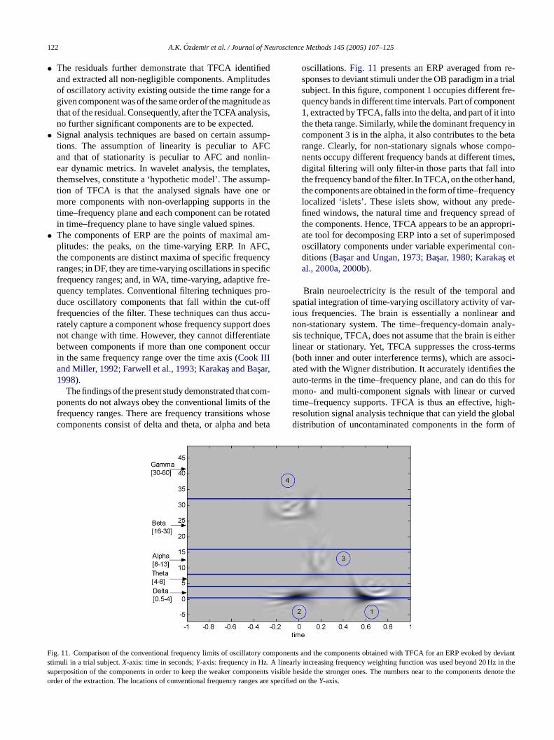
com-f thehosebeta
oscillations.Fig. 11 presents an ERP averaged from re-sponses to deviant stimuli under the OB paradigm in a trialsubject. In this figure, component 1 occupies different fre-quency bands in different time intervals. Part of component1, extracted by TFCA, falls into the delta, and part of it intothe theta range. Similarly, while the dominant frequency incomponent 3 is in the alpha, it also contributes to the betarange. Clearly, for non-stationary signals whose compo-nents occupy different frequency bands at different times,digital filtering will only filter-in those parts that fall intothe frequency band of the filter. In TFCA, on the other hand,the components are obtained in the form of time–frequencylocalized ‘islets’. These islets show, without any prede-fined windows, the natural time and frequency spread ofthe components. Hence, TFCA appears to be an appropri-ate tool for decomposing ERP into a set of superimposedoscillatory components under variable experimental con-ditions (Basar and Ungan, 1973; Bas¸ar, 1980; Karakas¸ etal., 2000a, 2000b).
Brain neuroelectricity is the result of the temporal andspatial integration of time-varying oscillatory activity of var-ious frequencies. The brain is essentially a nonlinear andnon-stationary system. The time–frequency-domain analy-sis technique, TFCA, does not assume that the brain is eitherlinear or stationary. Yet, TFCA suppresses the cross-terms( soci-a thea is form vedt igh-r lobald of
F y comp by deviants . A line in thes nents nts denote theo s are s
in the same frequency range over the time axis (Cook IIIand Miller, 1992; Farwell et al., 1993; Karakas¸ and Bas¸ar,1998).
The findings of the present study demonstrated thatponents do not always obey the conventional limits ofrequency ranges. There are frequency transitions wcomponents consist of delta and theta, or alpha and
ig. 11. Comparison of the conventional frequency limits of oscillatortimuli in a trial subject.X-axis: time in seconds;Y-axis: frequency in Hzuperposition of the components in order to keep the weaker comporder of the extraction. The locations of conventional frequency range
both inner and outer interference terms), which are asted with the Wigner distribution. It accurately identifiesuto-terms in the time–frequency plane, and can do thono- and multi-component signals with linear or cur
ime–frequency supports. TFCA is thus an effective, hesolution signal analysis technique that can yield the gistribution of uncontaminated components in the form
onents and the components obtained with TFCA for an ERP evokedarly increasing frequency weighting function was used beyond 20 Hzvisible beside the stronger ones. The numbers near to the componepecified on theY-axis.
A.K. Ozdemir et al. / Journal of Neuroscience Methods 145 (2005) 107–125 123
spatially and temporally integrated, time-varying oscillatoryactivity of various frequencies. TFCA seems therefore anappropriate tool for studying the intricate machinery of thehuman brain.
Recent work on brain neuroelectricity stresses the impor-tance of single sweep analysis.Jansen et al. (2003)pointedout that ensemble averages will not resemble single trialresponses. Likewise, single trial responses are not amplitudescaled versions of ensemble averages.Makeig (2002)showedthat by means of an adequate analysis of single trials, dynamicconsistencies between features of EEG averages (ERPs)and event-related changes in EEG signals can be found. Therecently developed piecewise Prony method (Garossi andJansen, 2000) has proven to be useful in decomposing non-stationary signals into a sum of oscillatory components withtime-varying frequency, amplitude, and phase characteristics.The method could show the temporal profile of poststimulussignal changes in single-trial evoked potentials. A goal forthe future studies should thus be to test the utility of TFCA onsingle sweep ERPs that have been obtained under differentparadigms, and in different states of consciousness. Suchstudies might help to gain new insights into the oscillatorydynamics of the brain during different cognitive operations.
R
A ysiol
A pre-
Als of
nualNS).
B rep-cess
B ency
B oked-
B les
B nc-nger-
B singsof
Bang
B :71–
B r thethe
Basar-Eroglu C, Basar E, Demiralp T, Schurmann M. P300-response:possible psychophysiological correlates in delta and theta frequencychannels. A review. Int J Psychophysiol 1992;13:161–79.
Berger H. Uber des elektroenkephalogram. Arch Psychiatry Nervenkr1929;87:527–70.
Boashash B, O’Shea P. Use of the cross Wigner–Ville distribution forestimation of instantaneous frequency. IEEE Trans Signal Process1993;41:1439–45.
Boudreaux-Bartels GF, Parks TW. Time-varying filtering and signal es-timation using Wigner distribution synthesis techniques. IEEE TransAcoust Speech Signal Process 1986(34):442–51.
Brandt ME, Jansen BH. The relationship between prestimulus alphaamplitude and visual evoked potential amplitude. Int J Neurosci1991;61:261–8.
Brown MK, Rabiner LR. An adaptive, ordered, graph search techniquefor dynamic time warping for isolated word recognition. IEEE TransAcoust Speech Signal Process 1982;30:535–44.
Coates M, Fitzgerald W. Time–frequency signal decomposition using en-ergy mixture models. Proc IEEE Int Conf Acoust Speech Signal Pro-cess 2000;II:633–6.
Choi HI, Williams WJ. Improved time–frequency representation of mul-ticomponent signals using exponential kernels. IEEE Trans AcoustSpeech Signal Process 1989;37:862–71.
Cohen L. Time–frequency distributions: a review. Proc IEEE 1989;77(7):941–81.
Cohen L. Time–frequency analysis. Englewood Cliffs, NJ: Prentice-Hall;1995.
Cook EW 3rd, Miller GA. Digital filtering: background and tutorial forpsychophysiologists. Psychophysiology 1992;29:350–67.
Czerwinski RN, Jones DL. Adaptive cone-kernel time–frequency analysis.IEEE Trans Signal Process 1995;43:1715–9.
D oked
D1–7.
D ofI:
inger-
Drain
D con-
D itiveGH,esses
D rop-cess
E tivetion.
F imalrain
G ewiseEng
H tribu-ignerster-
H mu-for
.
eferences
drian ED. Olfactory reactions in the brain of the hedgehog. J Ph1942;100:459–73.
lmeida LB. The fractional Fourier transform and time–frequency resentations. IEEE Trans Signal Process 1994;42:3084–91.
rıkan O, Ozdemir AK, Tufekci DI, Cakmak ED, Karakas¸ S. A newtechnique for joint time–frequency analysis of event-related signathe brain: time–frequency component analyzer (TFCA). Fifth AnConference of the EEG & Clinical Neuroscience Society (ECClin EEG Electroencephalogr 2003;34(3):170.
araniuk RG, Jones DL. A signal-dependent time–frequencyresentation: optimal kernel design. IEEE Trans Signal Pro1993;41:1589–601.
araniuk R, Coates M, Steeghs P. Hybrid linear/quadratic time–frequattributes. IEEE Trans Signal Process 2001;49:760–6.
asar E. EEG–brain dynamics: relation between EEG and brain evpotentials. Amsterdam: Elsevier; 1980.
asar E. Brain function and oscillations I: brain oscillations. Principand approaches. Heidelberg: Springer-Verlag; 1998.
asar E. Brain function and oscillations II: integrative brain fution. Neurophysiology and cognitive processes. Heidelberg: SpriVerlag; 1999.
asar E, Bas¸ar-Eroglu C, Karakas¸ S, Schurmann M. Brain oscillationin perception and memory. In: Chiarenza GA, editor. Proceedof the Ninth World Congress of the International OrganisationPsychophysiology, vol. 35; 2000. p. 95–124.
asar E, Demiralp T, Schurmann M, Bas¸ar-Eroglu C, Ademoglu A. Os-cillatory brain dynamics, wavelet analysis and cognition. Brain L1999;66(1):146–83.
asar E, Ozgoren M, Bas¸ar-Eroglu C, Karakas¸ S. Superbindingspatio-temporal oscillatory dynamics. Theory Biosci 2003;121:385.
asar E, Ungan P. A component analysis and principles derived founderstanding of the evoked potentials of the brain: studies inhippocampus. Kybernetik 1973;12:133–40.
awson GD. A summation technique for the detection of small evpotentials. Electroencephalogr Clin Neurophysiol 1954;6:65–84.
emiralp T, Ademoglu A, Istefanopulos Y, Bas¸ar-Eroglu C, Basar E.Wavelet analysis of oddball P300. Int J Psychophysiol 2001;39:22
emiralp T, Ademoglu A, Schurmann M, Bas¸ar E. Wavelet analysisbrain waves. In: Bas¸ar E, editor. Brain function and oscillationsbrain oscillations. Principles and approaches. Heidelberg: SprVerlag; 1998.
emiralp T, Ademoglu A, Schurmann M, Bas¸ar-Eroglu C, Basar E. De-tection of P300 in single trials by the wavelet transform (WT). BLang 1999;66:108–28.
onchin E, Coles MGH. Is the P300 component a manifestation oftext updating? Behav Brain Sci 1988;11:357–74.
onchin E, Karis D, Bashore TR, Coles MGH, Gratton G. Cognpsychophysiology and human information processing. In: Coles MDonchin E, Porges SW, editors. Psychophysiology: systems, procand applications. New York: Guilford Press; 1986. p. 244–66.
urak L, Arıkan O. Short-time Fourier transform: two fundamental perties and an optimal implementation. IEEE Trans Signal Pro2003;51(5):1231–42.
rden MF, Kutay MA, Ozaktas HM. Repeated filtering in consecufractional Fourier domains and its application to signal restoraIEEE Trans Signal Process 1999;47:1458–62.
arwell LA, Martinerie JM, Bashore TR, Rapp PE, Goddard PH. Optdigital filters for long-latency components of the event-related bpotential. Psychophysiology 1993;30:306–15.
arossi V, Jansen BH. Development and evaluation of the piecProny method for evoked potential analysis. IEEE Trans Biomed2000;47(12):1549–54.
lawatsch F, Flandrin P. The interference structure of the Wigner distion and related time–frequency signal representations. In: The Wdistribution—theory and applications in signal processing. Amdam: Elsevier; 1997 p. 59–133.
lawatsch F, Matz G, Kirchauer H, Kozek W. Time–frequency forlation, design, and implementation of time-varying optimal filterssignal estimation. IEEE Trans Signal Process 2000;48:1417–32
124 A.K. Ozdemir et al. / Journal of Neuroscience Methods 145 (2005) 107–125
Hlawatsch F, Kozek W. Time–frequency projection filters and time–frequency signal expansions. IEEE Trans Signal Process 1994;42:3321–34.
Hlawatsch F, Costa AH, Krattenthaler W. Time–frequency signal synthesiswith time–frequency extrapolation and don’t-care regions. IEEE TransSignal Process 1994;42:2513–20.
Humphreys DG, Kramer AF. Toward a psychophysiological assessmentof dynamic changes in mental overload. Hum Factors 1994;36:3–22.
Jansen B, Agarwal A, Hegde A, Boutros NN. Phase synchronizationof the ongoing EEG and auditory EP generation. Clin Neurophysiol2003;114:79–85.
Jervis BW, Nichols MJ, Johnson TE, Allen E, Hudson NR. A fundamentalinvestigation of the composition of auditory evoked potentials. IEEETrans Biomed Eng 1983;30:43–9.
Johnson R. The amplitude of the P300 component of the event-relatedpotentials: a review and synpaper. Advances in psychophysiology: aresearch annual, vol. 3. Greenwich: JAI Press; 1988.
Jones DL, Baraniuk RG. An adaptive optimal-kernel time–frequency rep-resentation. IEEE Trans Signal Process 1995;43:2361–71.
Kamarajan C, Porjesz B, Jones KA, Choi K, Chorlian DB, Padmanab-hapillai A. The role of brain oscillations as functional correlates ofcognitive systems: a study of frontal inhibitory control in alcoholism.Int J Psychophysiol 2004;51(2):155–80.
KarakasS. A descriptive framework for information processing: an in-tegrative approach. Brain alpha activity: new aspects and functionalcorrelates. Int J Psychophysiol 1997;26:353–68.
KarakasS, Basar E. Early gamma response is sensory in origin: a conclu-sion based on cross-comparison of results from multiple experimentalparadigms. Int J Psychophysiol 1998;31(1):13–31.
KarakasS, Erzengin OU, Bas¸ar E. A new strategy involving multiplecognitive paradigms demonstrates that ERP components are deter-
hys-
K re-blies.
K g theEE
K for29–
K pro-ential
K usingocess
M esneience
M elec-
M nalsribu-
M rans
M ntum
M rlin:
N of se-
N singres of
Naatanen R. Attention and brain function. London: Lawrence ErlbaumAssociates; 1992.
Naatanen R, Schroger E, Karakas¸ S, Tervaniemi M, Paavilainen P. Devel-opment of a memory trace for a complex sound in the human brain.Neuroreport 1993;4:503–6.
Ozaktas HM, Arıkan O, Kutay MA, Bozdagi G. Digital computa-tion of the fractional Fourier transform. IEEE Trans Signal Process1996;44:2141–50.
Ozdemir AK. Time–frequency component analyzer. Unpublished doctoraldissertation, Bilkent University, Ankara, Turkey, 2003.
Ozdemir AK, Arıkan O. Efficient computation of the ambiguity functionand Wigner distribution on arbitrary line segments. IEEE Trans SignalProcess 2001;49:381–93.
Ozdemir AK, Arıkan O. A high-resolution time–frequency representationwith significantly reduced cross-terms. Proc IEEE Int Conf AcoustSpeech Signal Process 2000;2:693–6.
Ozdemir AK, Durak L, Arıkan O. High-resolution time–frequency anal-ysis based on fractional domain warping. Proc IEEE Int Conf AcoustSpeech Signal Process 2001;6:3553–6.
Page CH. Instantaneous power spectra. J Appl Phys 1952;23:103–6.Parvin C, Torres F, Johnson E. Synchronization of single evoked response
components: estimation and interrelation of reproducibility measures.In: Rhythmic EEG activities and cortical functioning. Amsterdam:Elsevier; 1980.
Picton TW, editor. Human event-related potentials. Handbook of elec-troencephalography and clinical neurophysiology. Amsterdam: Else-vier; 1988.
Picton TW, Hillyard SA, Krausz HI, Galambos R. Human auditory evokedpotentials. I. Evaluation of components. Electroencephalogr Clin Neu-rophysiol 1974;36:176–90.
Polich J, Kok A. Cognitive and biological determinants of P300: an in-
P ball169–
P d T.manSA
R KA,atry
R man. Int
R amsf au-06–
R ,rain
R lysisiods.
S aly-ang
S rain:ysiol
S itory
S atic
S es of
mined by the superposition of oscillatory responses. Clin Neuropiol 2000a;111:1719–32.
arakasS, Erzengin OU, Bas¸ar E. The genesis of human event-relatedsponses explained through the theory of oscillatory neural assemNeurosci Lett 2000b;285:45–8.
atkovnik V, Stankovic L. Instantaneous frequency estimation usinWigner distribution with varying data-driven window length. IETrans Signal Process 1998;46:3215–25.
olev V, Yordanova J. Analysis of phase-locking is informativestudying event-related EEG activity. Biol Cybern 1997;96:235.
ramer AF, Strayer DL. Assessing the development of automaticcessing: an application of dual-track and event-related brain potmethodologies. Biol Psychol 1988;26:231–67.
wok HK, Jones DL. Improved instantaneous frequency estimationan adaptive short-time Fourier transform. IEEE Trans Signal Pr2000;48:2964–72.
akeig S, Westerfield M, Jung TP, Enghoff S, Townsend J, CourchE, et al. Dynamic brain sources of visual evoked responses. Sc2002;295(5555):690–4.
akeig S. Response: event-related brain dynamics-unifying braintrophysiology. Trends Neurosci 2002;25(8):390.
cHale TJ, Boudreaux-Bartels GF. An algorithm for synthesizing sigfrom partial time–frequency models using the cross Wigner disttion. IEEE Trans Signal Process 1993;41(5):1986–90.
eda N. Transversal filters with nonuniform tap spacing. IEEE TCircuits Syst 1980;27:1–11.
ergenau H, Hill RN. Correlation between measurements in quatheory. Prog Theor Phys 1961;26:722–38.
ountcastle V. Preface. In: Induced rhythms of the brain. BeBirkhauser; 1992.
aatanen R. Processing negativity: an evoked potential reflectionlective attention. Psychol Bull 1982;92(3):605–40.
aatanen R. The role of attention in auditory information procesas revealed by event-related potentials and other brain measucognitive function. Behav Brain Sci 1990;13(2):201–88.
tegrative review. Biol Psychol 1995;41:103–46.olich J, Margala C. P300 and probability: comparison of odd
and single stimulus paradigms. Int J Psychophysiol 1997;25:76.
orjesz B, Almasy L, Edenberg HJ, Wang K, Chorlian DB, ForouLinkage disequilibrium between the beta frequency of the huEEG and a GABAA receptor gene locus. Proc Natl Acad Sci U2002;99(6):3729–33.
angaswamy M, Porjesz B, Chorlian DB, Wang K, JonesBauer LO. Beta power in the EEG of alcoholics. Biol Psychi2002;52(8):831–42.
angaswamy M, Porjesz B, Chorlian DB, Wang K, Jones KA, KuperS. Resting EEG in offspring of male alcoholics: beta frequenciesJ Psychophysiol 2004;51(3):239–51.
itter W, Paavilainen P, Lavikainen J, Reinikainen K, Alho K, SM, et al. Event-related potentials to repetition and change oditory stimuli. Electroencephalogr Clin Neurophysiol 1992;83:321.
osso OA, Blanco S, Yordanova J, Kolev V, Figliola A, Schurmann Met al. Wavelet entropy: a new tool for analysis of short-duration belectrical signals. J Neurosci Methods 2001;105:65–75.
oschke J, Mann K, Riemann D, Frank C, Fell J. Sequential anaof the brain’s transfer properties during consecutive REM perElectroencephalogr Clin Neurophysiol 1995;96:390–7.
amar V, Bobardikar A, Raghuveer MR, Swarz K. Wavelet ansis of neuro-electric waveforms: a conceptual tutorial. Brain L1999;66:7–60.
annita WG. Stimulus-specific oscillatory responses of the ba time/frequency-related coding process. Clin Neuroph2000;111(4):565–83.
ayers BM, Beagley HA, Henshall WR. The mechanism of audevoked EEG responses. Nature 1974;247(15):481–3.
olodovnikov VV. Introduction to the statistical dynamics of automcontrol systems. New York: Dover; 1960.
utton S, Braren M, Zubin J, John ER. Evoked potential correlatstimulus uncertainty. Science 1965;150:1187–8.
A.K. Ozdemir et al. / Journal of Neuroscience Methods 145 (2005) 107–125 125
Tagluk ME, Cakmak ED, Karakas¸ S. Analysis of time-varying energy ofbrain responses to an oddball paradigm using short-term smoothedWigner–Ville distribution. Int J Neurosci, in press.
Tagluk ME, Cakmak ED, Karakas¸ S. High resolution energy distribu-tion of brain electrical activity obtained under the oddball paradigm.BIOMUT May 2002;239:13–9.
Tervaniemi M, Saarinen J, Paavilainen P, Danilova N, Naatanen R.Evoked potential correlates of stimulus uncertainty. Biol Psychol1994;38:157–67.
Vincent L, Soille P. Watersheds in digital spaces: an efficient algorithmbased on immersion simulations. IEEE Trans Pattern Anal Mach Intell1991;13(6):583–98.
Wickens C, Kramer A, Vanasse L, Dionchin E. The performanceof concurrent task: a psychophysiological analysis of the reci-
procity of information processing resources. Science 1983;221:1080–2.
Winkler I, Paavilainen P, Naatanen R. Can echoic memory store twotraces simultaneously? A study of event-related brain potentials. Psy-chophysiology 1992;29(3):337–49.
Wulich D, Plotkin EI, Swamy MNS. Synpaper of discrete time-varyingnull filters for frequency-varying signals using the time-warping tech-nique. IEEE Trans Circuits Syst 1990;37:977–90.
Yordanova J, Kolev V. A single sweep analysis of the theta frequency bandduring auditory oddball task. Psychophysiology 1998;35(1):116–26.
Yordonova J, Kolev V, Rosso OA, Schurmann M, Sokowitz OW,OzgorenM, et al. Wavelet entropy analysis of event-related potentials indi-cates modality of independent theta dominance. J Neurosci Methods2002;117:99–109.