Embed Size (px)
Citation preview
LUDWIG-MAXIMILIANS UNIVERSITÄT MÜNCHEN
MASTER THESIS
Timing Calibration of the ATLAS MuonSpectrometer for a Search for charged
stable massive Particles with Run–2 data
Author:Philipp SEIFERMANN
Supervisor:Dr. habil. Sascha MEHLHASE
A thesis submitted in fulfillment of the requirementsfor the degree of Master of Physics
in the
Faculty of PhysicsElementary Particle Physics
August 18, 2020

LUDWIG-MAXIMILIANS UNIVERSITÄT MÜNCHEN
MASTERARBEIT
Kalibration der Zeitmessung des ATLASMuonspektromters für eine Suche nach
geladenen stabilen massiven Teilchen mitdem Run–2 Datensatz
Author:Philipp SEIFERMANN
Supervisor:Dr. habil. Sascha MEHLHASE
Eine Masterarbeit erarbeitet im Zugedes Masterprogramms
an der
Fakultät für PhysikElementarteilchenphysik
August 18, 2020

iii
LUDWIG-MAXIMILIANS UNIVERSITÄT MÜNCHEN
AbstractFaculty of Physics
Elementary Particle Physics
Master of Physics
Timing Calibration of the ATLAS Muon Spectrometer for a Search for chargedstable massive Particles with Run–2 data
by Philipp SEIFERMANN
A timing calibration of the ATLAS Muon Spectrometer with 139 fb−1 of proton–proton collisions at
√s = 13 TeV during Run–2 is presented in the context of a search
for charged stable massive particles. Charged stable massive particles leave the sig-nature of heavy muon-like particles. Due to the their high mass, they are expectedto traverse the detector at speeds well below the speed of light and thus offer amodel-independent approach to observe New Physics. The low velocity manifestsas long time-of-flight values, especially in the outer parts of the detector. The timingmeasurement of the muon spectrometer is thus an important variable for the identi-fication of charged stable massive particles. A calibration procedure for the timingmeasurement is therefore necessary, involving calibration constants for over 725,000individual detector elements.


v
AcknowledgementsWithout the help and support of several people this master’s thesis could not havebeen done. To anyone who supported me during the time it took to complete thiswork, I want to express my sincere gratitude.Nevertheless, some people deserve to be mentioned specifically.
The first person I need to thank is Dr. habil. Sascha Mehlhase for his supervisionof this thesis. Without his help this thesis would not have been possible. I want toespecially emphasize the warm and positive attitude he nourished during my timein his research group.
Further, I am thankful to Prof. Dr. Dorothee Schaile for the opportunity to writethis thesis at her chair in the first place and the kind and helpful work environmentshe fostered at her chair. Additionally, I would like to thank her for the possibility tovisit CERN and ATLAS itself.
A special thanks to Ferdinand Krieter, who not only provided some of the frame-work used for this work but was also always willing to offer his support with anysort of problem that arose.
More generally, I would like to thank every member of the LS Schaile for the greatwork environment, joint lunches and occasional ping-pong breaks. I am lucky tosay, that I could spend the time in such a kind-hearted and helpful atmosphere.
To Joschua Krink I want to express my sincere gratitude for almost six years offriendship. I am not sure how my academic studies would have evolved withouthim and the other members of the BlankoBlattBande. Especially as the usual workenvironment was not available any more, due to the Corona pandemic, the help heprovided within the little office we set up was essential for finishing this work.
Last, but surely not least, I want to thank my family for the constant support I re-ceived during my studies and the time it took to write this thesis.

vii
Contents
Abstract iii
Acknowledgements v
1 Introduction 1
2 Theory 32.1 The Standard Model of Particle Physics . . . . . . . . . . . . . . . . . . 3
2.1.1 Elementary Particles . . . . . . . . . . . . . . . . . . . . . . . . . 32.1.2 Interactions . . . . . . . . . . . . . . . . . . . . . . . . . . . . . . 6
2.2 Lifetime of Particles . . . . . . . . . . . . . . . . . . . . . . . . . . . . . . 102.3 The need for New Physics . . . . . . . . . . . . . . . . . . . . . . . . . . 122.4 Beyond the Standard Model . . . . . . . . . . . . . . . . . . . . . . . . . 142.5 Summary . . . . . . . . . . . . . . . . . . . . . . . . . . . . . . . . . . . . 18
3 The Experiment 193.1 The Large Hadron Collider . . . . . . . . . . . . . . . . . . . . . . . . . 193.2 The ATLAS Detector . . . . . . . . . . . . . . . . . . . . . . . . . . . . . 22
3.2.1 Inner Detector . . . . . . . . . . . . . . . . . . . . . . . . . . . . . 253.2.2 Calorimeters . . . . . . . . . . . . . . . . . . . . . . . . . . . . . . 273.2.3 Muon Spectrometer . . . . . . . . . . . . . . . . . . . . . . . . . 28
4 Charged Stable Massive Particles at ATLAS 354.1 Production . . . . . . . . . . . . . . . . . . . . . . . . . . . . . . . . . . . 354.2 Observables . . . . . . . . . . . . . . . . . . . . . . . . . . . . . . . . . . 36
4.2.1 Ionisation Energy Loss . . . . . . . . . . . . . . . . . . . . . . . . 364.2.2 Time-of-Flight Measurement . . . . . . . . . . . . . . . . . . . . 37
4.3 Muon Reconstruction . . . . . . . . . . . . . . . . . . . . . . . . . . . . . 38
5 Calibration of the Timing Measurement of the ATLAS Muon Spectrometer 415.1 Data and Event Selection . . . . . . . . . . . . . . . . . . . . . . . . . . . 425.2 Uncalibrated Distributions . . . . . . . . . . . . . . . . . . . . . . . . . . 425.3 Run-wise Calibration . . . . . . . . . . . . . . . . . . . . . . . . . . . . . 465.4 Element-wise Calibration . . . . . . . . . . . . . . . . . . . . . . . . . . 505.5 Drift-time Calibration . . . . . . . . . . . . . . . . . . . . . . . . . . . . . 535.6 Phi Calibration . . . . . . . . . . . . . . . . . . . . . . . . . . . . . . . . 555.7 Final β Resolution and Pull . . . . . . . . . . . . . . . . . . . . . . . . . 61
6 Conclusion and Outlook 65
Bibliography 67
Declaration of Authorship 77

1
Chapter 1
Introduction
The general idea of elementary particle physics is to provide a description of the in-teractions between the smallest units that matter is build of in our universe. Over theyears physicists provided continuous improvements to that description. Through-out the last decades a framework called the Standard Model of particle physicsemerged as the leading theory. The Standard Model had huge success and waseven able to predict particles exceeding the technological capabilities of detectionat the time. With the discovery of the Higgs boson in 2012 [1, 2], the last remainingpuzzle peace of the Standard Model was found. Even though the Standard Modelwas successfully tested throughout the years, it is known to be limited in its ex-planatory power. Indeed more and more observations in and outside the realm ofparticle physics occur, that can not be fully explained within the Standard Model.First and foremost a coherent implementation of gravity is not included inside theStandard Model. In addition, the Standard model is neither capable of providinga suitable dark matter candidate, needed to explain astrophysical and cosmologicalobservations, nor is it able to explain the observed difference between anti-matterand matter observed in our universe.
Therefore, a variety of of theories Beyond the Standard Model (BSM), also calledNew Physics, are proposed aiming at resolving one or several shortcomings of theStandard Model. So far no one-fits-all solution was able to emerge, which allowsfor open-mindedness in the search for New Physics. However, many of these newtheories include the existence of new particles, which could be created at particlescolliders and be detected with modern detectors. As indications of their existencewould have already been found, if these particles would have masses comparableto Standard Model particles, they are usually predicted with masses exceeding therange of Standard Model masses. The mechanisms that result in some long-livingparticles in the Standard Model, could similarly lead to new particles being eitherstable or having a life-time long enough to traverse the detector. Many proposed the-ories include such long-living particles carrying an electric charge, which are there-fore called charged stable massive particles in this work.
Charged stable massive particles offer an interesting approach to a search for NewPhysics. Because of their charge and long life-time, they can be observed directly bya particle detector and not via the reconstruction of their decay. This autonomy ofthe specific decay process makes the search model-independent, as the exact produc-tion and decay process must not be known. Due to their large mass and availableelectromagnetic charge, a charged stable massive particle traversing a particle de-tector would suffer a large ionisation energy loss and would propagate through thedetector with a velocity significantly slower than the speed of light. By measuringthe time it took the traversing particle to reach the detector element it interacted
2 Chapter 1. Introduction
with, this velocity can be obtained. In addition to the model-independence, thesesearches have little to no Standard Model background because no Standard Modelparticle would leave such a signature. This leads to the detector mismeasurementsbeing the main background that has to be considered for such an analysis. A clearunderstanding and a thorough calibration of the detector system used in the searchis therefore necessary.
Within the ATLAS Collaboration, multiple searches for charged stable massive parti-cles were conducted so far but none observed a significant excess over the estimatedbackground. To gather information about the energy loss through ionisation the In-ner Detector of ATLAS can be used and for a time-of-flight measurement the tilecalorimeter, as well as the monitored drift tubes and resistive plate chambers of theMuon Spectrometer, can be used. The work at hand focuses on a timing calibrationof the latter two detector parts placed in the outermost region of the detector usingthe data taken by ATLAS during Run–2 with a centre-of-mass energy of
√s = 13
TeV. The thesis is structured as follows: in Chapter 2 an introduction of the theoreti-cal framework of the Standard Model is given and the need for a search for chargedstable massive particles is motivated. Chapter 3 introduces the experimental setup atCERN with focus on the LHC and ATLAS. The characteristics of charged stable mas-sive particles at ATLAS are introduced in Chapter 4. Chapter 5 details the calibrationprocedure deployed in this work, as well as their effects on the timing measurementand the final resolution of the velocity. In the final Chapter 6 a conclusion and anoutlook are given.
3
Chapter 2
Theory
The foundation of modern particle physics is given by the Standard Model. It de-scribes the elemental building blocks of nature and three of the four known fun-damental interactions in physics through quantum field theories. Even though theStandard Model is one of the best validated theories in physics, there are alreadyknown limitations in the applicability of it. Therefore, theorists have been imagin-ing theories superseding the Standard Model for a while.The following chapter will give a brief introduction into the particle content of theStandard Model and the interactions it describes. Since the work at hand focuses onlong-lived particles in the context of New Physics, the subject of longevity will beaddressed shortly, as well as the limitations of the Standard Model, and the need fora BSM theory will be motivated.In this work, the for particle physics usual convention of c := h := 1 is used.
2.1 The Standard Model of Particle Physics
The Standard Model describes all known building blocks of matter and their inter-actions through three of the four known fundamental forces, which are the electro-magnetic, weak, strong and gravitational force. A proper description of gravity, inthe context of a quantum field theory, has not been successful so far, and therefore,it is not included in the Standard Model. Even though gravity is dominant on largescales and consequently essential in fields like astrophysics, on small scales and atlow energies, the effects of gravity are inconsequential compared to the effects of theother three forces and thus negligible in today’s particle physics. Therefore, the ab-sence of gravity does not entail a major detriment on the effectiveness of predictionsmade by the Standard Model. The fundamental building blocks and the particlesthat mediate the forces are assumed to be point-like, which means they do not havean inner structure and are thus called elementary particles. References [3, 4] givecomprehensive introductions into the Standard Model and were used as inspirationsfor much of this chapter.
2.1.1 Elementary Particles
Elementary particles can be split into two major groups according to their spin. Onthe one hand, there are fermions which have half-integer spin and are the buildingblocks of matter. On the other hand, there are bosons, which have integer spin. Theyact as the mediators of the forces and are responsible for the particles attaining theirmasses.
4 Chapter 2. Theory
Fermions
Fermions are further divided into three generations, where each partner of a highergeneration has a higher mass but is the same otherwise. Furthermore, they can bedivided according to their behaviour towards the strong interaction. Leptons areparticles without the charge necessary for the strong interaction and thus do nottake part in it. On the contrary, quarks have a colour charge and consequently dotake part in the strong interaction. There are six different types of leptons gatheredinto two groups with three elements, respectively. Charged leptons have an electriccharge of−1e, where e is the elementary charge1 and contain the electron (e−), muon(µ−) and tauon (τ−). The neutral leptons have fittingly an electric charge of 0 andencompass the electron neutrino (νe), muon neutrino (νµ) and tauon neutrino (ντ).
Within each generation of leptons, there is a pair of one charged and one neutrallepton. The first generation consists of the combination of electron and electronneutrino (e−,νe), the second generation contains the muon and the muon neutrino(µ−,νµ) and the third generation encloses the tauon and the tauon neutrino (τ−,ντ).Similar to leptons, quarks come in in three generations with two elements each. Oneelement is an up-type quark and the other is a down-type quark. Each up-type quarkcarries an electric charge of 2
3 e and one of the three colour charges red (r), blue (b)or green (g). The three different up-type flavours are called up (u), charm (c) andtop (t). The three down-type quarks, down (d), strange (s) and bottom (b), possesan electric charge of − 1
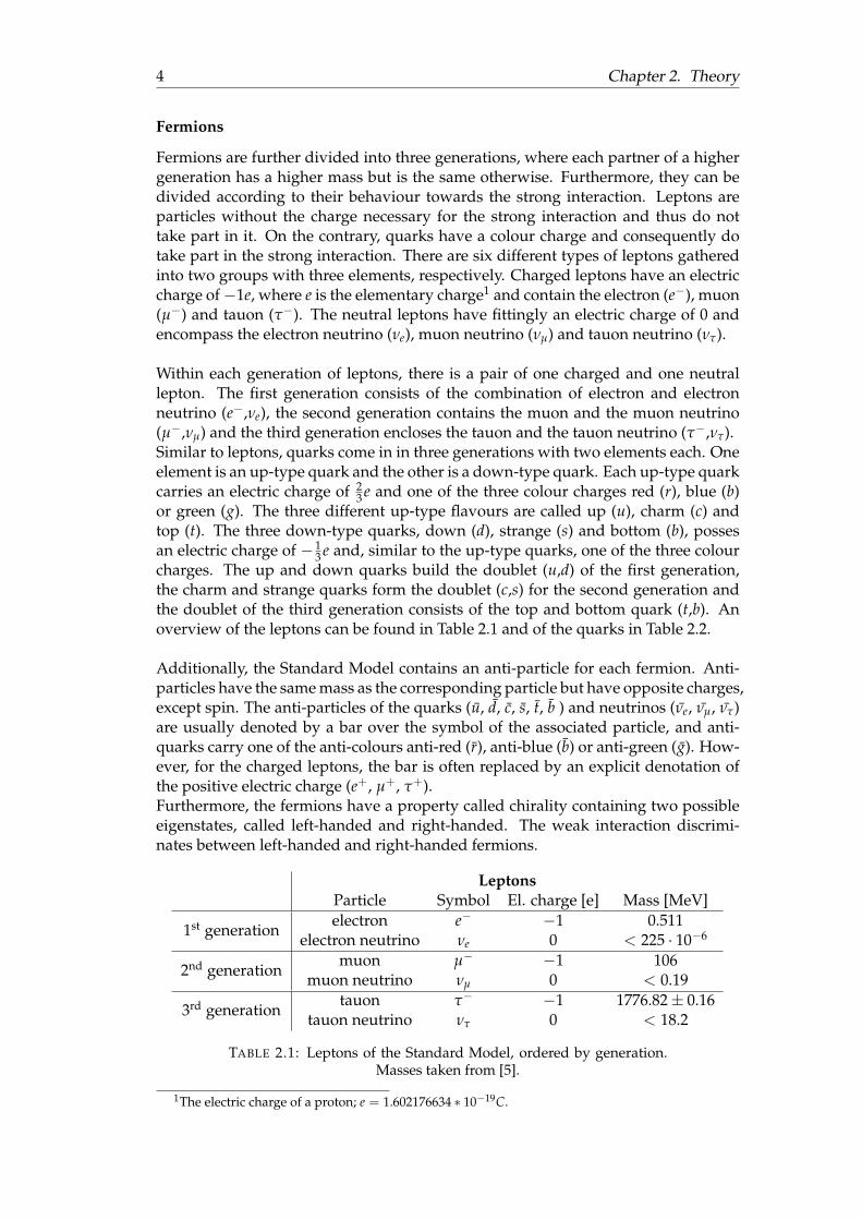
3 e and, similar to the up-type quarks, one of the three colourcharges. The up and down quarks build the doublet (u,d) of the first generation,the charm and strange quarks form the doublet (c,s) for the second generation andthe doublet of the third generation consists of the top and bottom quark (t,b). Anoverview of the leptons can be found in Table 2.1 and of the quarks in Table 2.2.
Additionally, the Standard Model contains an anti-particle for each fermion. Anti-particles have the same mass as the corresponding particle but have opposite charges,except spin. The anti-particles of the quarks (u, d, c, s, t, b ) and neutrinos (νe, νµ, ντ)are usually denoted by a bar over the symbol of the associated particle, and anti-quarks carry one of the anti-colours anti-red (r), anti-blue (b) or anti-green (g). How-ever, for the charged leptons, the bar is often replaced by an explicit denotation ofthe positive electric charge (e+, µ+, τ+).Furthermore, the fermions have a property called chirality containing two possibleeigenstates, called left-handed and right-handed. The weak interaction discrimi-nates between left-handed and right-handed fermions.
LeptonsParticle Symbol El. charge [e] Mass [MeV]
1st generationelectron e− −1 0.511
electron neutrino νe 0 < 225 · 10−6
2nd generationmuon µ− −1 106
muon neutrino νµ 0 < 0.19
3rd generationtauon τ− −1 1776.82± 0.16
tauon neutrino ντ 0 < 18.2
TABLE 2.1: Leptons of the Standard Model, ordered by generation.Masses taken from [5].
1The electric charge of a proton; e = 1.602176634 ∗ 10−19C.
2.1. The Standard Model of Particle Physics 5
QuarksParticle Symbol El. charge [e] Mass [MeV]
1st generationup u +2/3 2.3+0.7
−0.5down d −1/3 4.8+0.5
−0.3
2nd generationcharm c +2/3 (1.275± 0.025) · 103
strange s −1/3 95± 5
3rd generationtop t +2/3 (173.21± 1.22) · 103
bottom b −1/3 (4.25± 0.15) · 103
TABLE 2.2: Quarks of the Standard Model, ordered by generation.Masses taken from [5].
Bosons
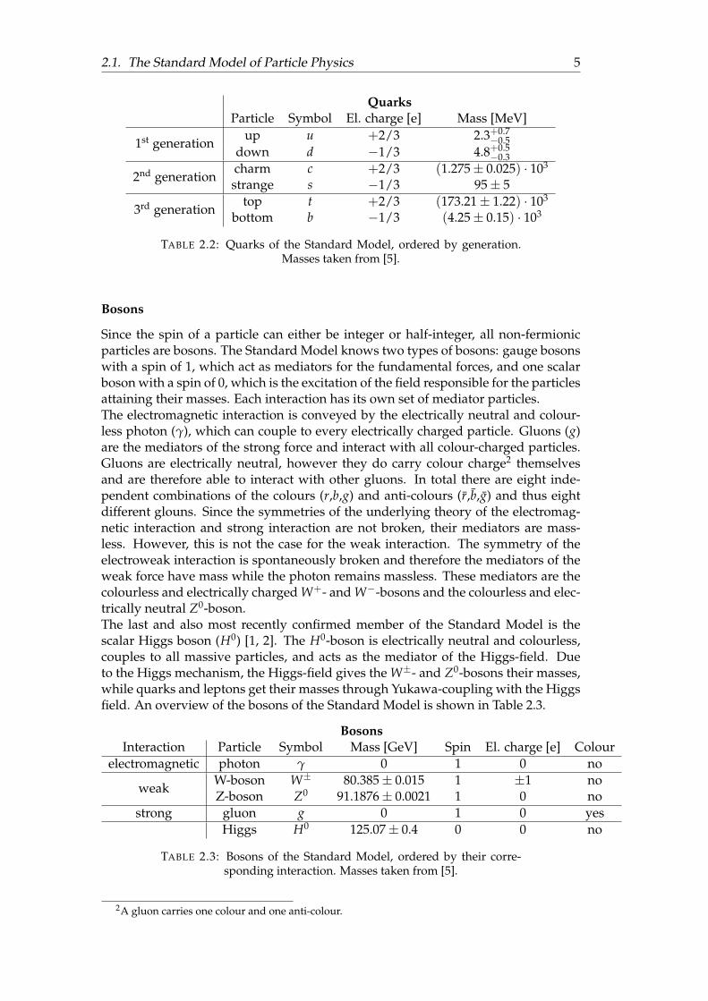
Since the spin of a particle can either be integer or half-integer, all non-fermionicparticles are bosons. The Standard Model knows two types of bosons: gauge bosonswith a spin of 1, which act as mediators for the fundamental forces, and one scalarboson with a spin of 0, which is the excitation of the field responsible for the particlesattaining their masses. Each interaction has its own set of mediator particles.The electromagnetic interaction is conveyed by the electrically neutral and colour-less photon (γ), which can couple to every electrically charged particle. Gluons (g)are the mediators of the strong force and interact with all colour-charged particles.Gluons are electrically neutral, however they do carry colour charge2 themselvesand are therefore able to interact with other gluons. In total there are eight inde-pendent combinations of the colours (r,b,g) and anti-colours (r,b,g) and thus eightdifferent glouns. Since the symmetries of the underlying theory of the electromag-netic interaction and strong interaction are not broken, their mediators are mass-less. However, this is not the case for the weak interaction. The symmetry of theelectroweak interaction is spontaneously broken and therefore the mediators of theweak force have mass while the photon remains massless. These mediators are thecolourless and electrically charged W+- and W−-bosons and the colourless and elec-trically neutral Z0-boson.The last and also most recently confirmed member of the Standard Model is thescalar Higgs boson (H0) [1, 2]. The H0-boson is electrically neutral and colourless,couples to all massive particles, and acts as the mediator of the Higgs-field. Dueto the Higgs mechanism, the Higgs-field gives the W±- and Z0-bosons their masses,while quarks and leptons get their masses through Yukawa-coupling with the Higgsfield. An overview of the bosons of the Standard Model is shown in Table 2.3.
BosonsInteraction Particle Symbol Mass [GeV] Spin El. charge [e] Colour
electromagnetic photon γ 0 1 0 no
weakW-boson W± 80.385± 0.015 1 ±1 noZ-boson Z0 91.1876± 0.0021 1 0 no
strong gluon g 0 1 0 yesHiggs H0 125.07± 0.4 0 0 no
TABLE 2.3: Bosons of the Standard Model, ordered by their corre-sponding interaction. Masses taken from [5].
2A gluon carries one colour and one anti-colour.
6 Chapter 2. Theory
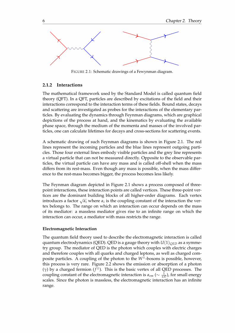
FIGURE 2.1: Schematic drawings of a Fewynman diagram.
2.1.2 Interactions
The mathematical framework used by the Standard Model is called quantum fieldtheory (QFT). In a QFT, particles are described by excitations of the field and theirinteractions correspond to the interaction terms of these fields. Bound states, decaysand scattering are investigated as probes for the interactions of the elementary par-ticles. By evaluating the dynamics through Feynman diagrams, which are graphicaldepictions of the process at hand, and the kinematics by evaluating the availablephase space, through the medium of the momenta and masses of the involved par-ticles, one can calculate lifetimes for decays and cross-sections for scattering events.
A schematic drawing of such Feynman diagrams is shown in Figure 2.1. The redlines represent the incoming particles and the blue lines represent outgoing parti-cles. Those four external lines embody visible particles and the grey line representsa virtual particle that can not be measured directly. Opposite to the observable par-ticles, the virtual particle can have any mass and is called off-shell when the massdiffers from its rest-mass. Even though any mass is possible, when the mass differ-ence to the rest-mass becomes bigger, the process becomes less likely.
The Feynman diagram depicted in Figure 2.1 shows a process composed of three-point interactions, these interaction points are called vertices. These three-point ver-tices are the dominant building blocks of all higher-order diagrams. Each vertexintroduces a factor
√αi where αi is the coupling constant of the interaction the ver-
tex belongs to. The range on which an interaction can occur depends on the massof its mediator: a massless mediator gives rise to an infinite range on which theinteraction can occur, a mediator with mass restricts the range.
Electromagnetic Interaction
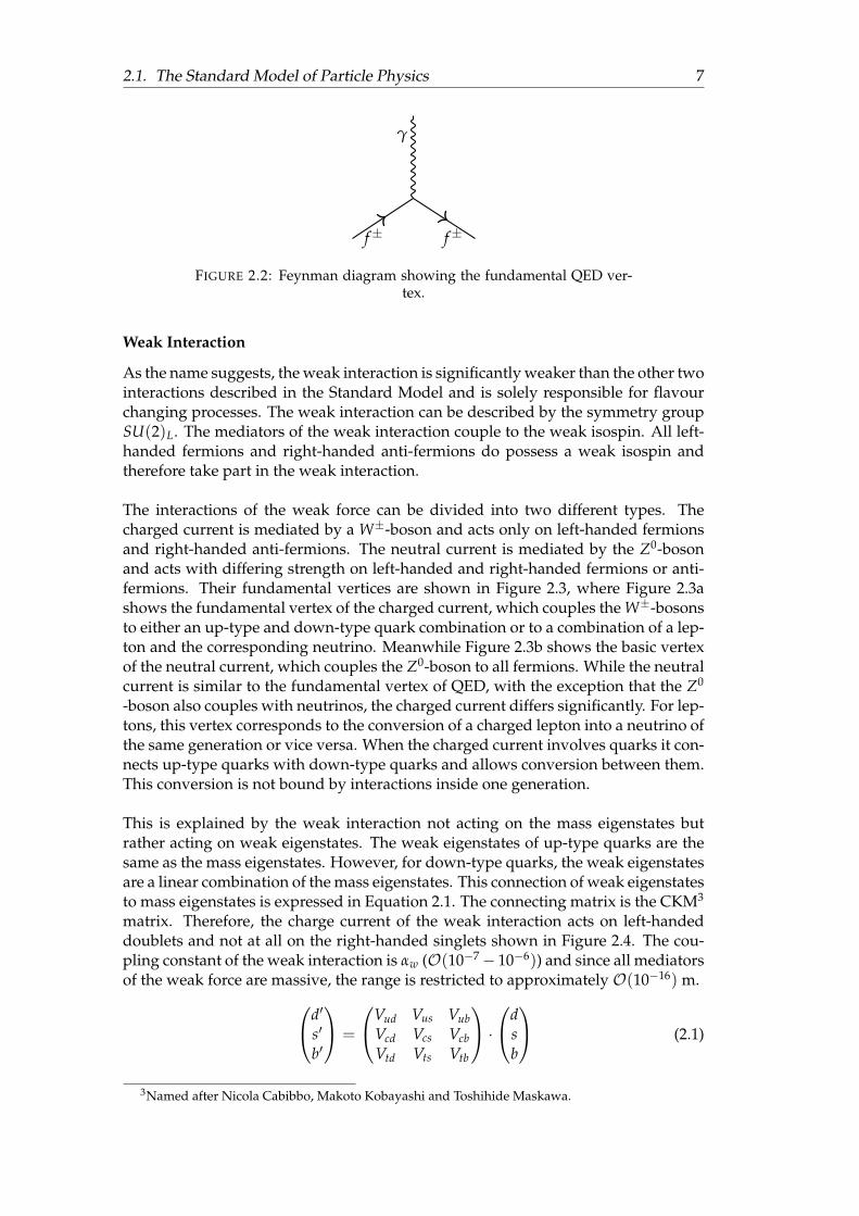
The quantum field theory used to describe the electromagnetic interaction is calledquantum electrodynamics (QED). QED is a gauge theory with U(1)QED as a symme-try group. The mediator of QED is the photon which couples with electric chargesand therefore couples with all quarks and charged leptons, as well as charged com-posite particles. A coupling of the photon to the W±-bosons is possible, however,this process is very rare. Figure 2.2 shows the emission or absorption of a photon(γ) by a charged fermion ( f±). This is the basic vertex of all QED processes. Thecoupling constant of the electromagnetic interaction is αem (∼ 1
137 ), for small energyscales. Since the photon is massless, the electromagnetic interaction has an infiniterange.
2.1. The Standard Model of Particle Physics 7
f± f±
γ
FIGURE 2.2: Feynman diagram showing the fundamental QED ver-tex.
Weak Interaction
As the name suggests, the weak interaction is significantly weaker than the other twointeractions described in the Standard Model and is solely responsible for flavourchanging processes. The weak interaction can be described by the symmetry groupSU(2)L. The mediators of the weak interaction couple to the weak isospin. All left-handed fermions and right-handed anti-fermions do possess a weak isospin andtherefore take part in the weak interaction.
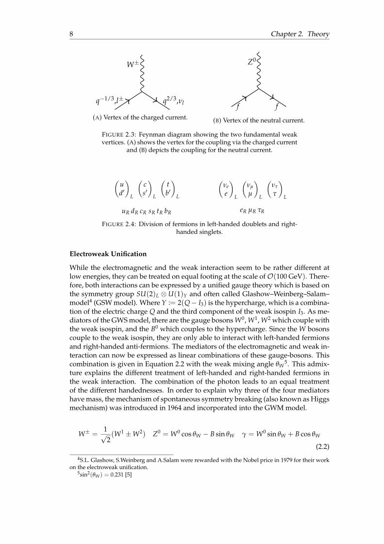
The interactions of the weak force can be divided into two different types. Thecharged current is mediated by a W±-boson and acts only on left-handed fermionsand right-handed anti-fermions. The neutral current is mediated by the Z0-bosonand acts with differing strength on left-handed and right-handed fermions or anti-fermions. Their fundamental vertices are shown in Figure 2.3, where Figure 2.3ashows the fundamental vertex of the charged current, which couples the W±-bosonsto either an up-type and down-type quark combination or to a combination of a lep-ton and the corresponding neutrino. Meanwhile Figure 2.3b shows the basic vertexof the neutral current, which couples the Z0-boson to all fermions. While the neutralcurrent is similar to the fundamental vertex of QED, with the exception that the Z0
-boson also couples with neutrinos, the charged current differs significantly. For lep-tons, this vertex corresponds to the conversion of a charged lepton into a neutrino ofthe same generation or vice versa. When the charged current involves quarks it con-nects up-type quarks with down-type quarks and allows conversion between them.This conversion is not bound by interactions inside one generation.
This is explained by the weak interaction not acting on the mass eigenstates butrather acting on weak eigenstates. The weak eigenstates of up-type quarks are thesame as the mass eigenstates. However, for down-type quarks, the weak eigenstatesare a linear combination of the mass eigenstates. This connection of weak eigenstatesto mass eigenstates is expressed in Equation 2.1. The connecting matrix is the CKM3
matrix. Therefore, the charge current of the weak interaction acts on left-handeddoublets and not at all on the right-handed singlets shown in Figure 2.4. The cou-pling constant of the weak interaction is αw (O(10−7− 10−6)) and since all mediatorsof the weak force are massive, the range is restricted to approximately O(10−16) m.d′
s′
b′
=
Vud Vus VubVcd Vcs VcbVtd Vts Vtb
·d
sb
(2.1)
3Named after Nicola Cabibbo, Makoto Kobayashi and Toshihide Maskawa.
8 Chapter 2. Theory
q−1/3,l± q2/3,νl
W±
(A) Vertex of the charged current.
f f
Z0
(B) Vertex of the neutral current.
FIGURE 2.3: Feynman diagram showing the two fundamental weakvertices. (A) shows the vertex for the coupling via the charged current
and (B) depicts the coupling for the neutral current.
(ud′
)L
(cs′
)L
(tb′
)L
uR dR cR sR tR bR
(νee
)L
(νµ
µ
)L
(ντ
τ
)L
eR µR τR
FIGURE 2.4: Division of fermions in left-handed doublets and right-handed singlets.
Electroweak Unification
While the electromagnetic and the weak interaction seem to be rather different atlow energies, they can be treated on equal footing at the scale ofO(100 GeV). There-fore, both interactions can be expressed by a unified gauge theory which is based onthe symmetry group SU(2)L ⊗U(1)Y and often called Glashow–Weinberg–Salam–model4 (GSW model). Where Y := 2(Q− I3) is the hypercharge, which is a combina-tion of the electric charge Q and the third component of the weak isospin I3. As me-diators of the GWS model, there are the gauge bosons W0, W1, W2 which couple withthe weak isospin, and the B0 which couples to the hypercharge. Since the W bosonscouple to the weak isospin, they are only able to interact with left-handed fermionsand right-handed anti-fermions. The mediators of the electromagnetic and weak in-teraction can now be expressed as linear combinations of these gauge-bosons. Thiscombination is given in Equation 2.2 with the weak mixing angle θW
5. This admix-ture explains the different treatment of left-handed and right-handed fermions inthe weak interaction. The combination of the photon leads to an equal treatmentof the different handednesses. In order to explain why three of the four mediatorshave mass, the mechanism of spontaneous symmetry breaking (also known as Higgsmechanism) was introduced in 1964 and incorporated into the GWM model.
W± =1√2(W1 ±W2) Z0 = W0 cos θW − B sin θW γ = W0 sin θW + B cos θW
(2.2)
4S.L. Glashow, S.Weinberg and A.Salam were rewarded with the Nobel price in 1979 for their workon the electroweak unification.
5sin2(θW) = 0.231 [5]
2.1. The Standard Model of Particle Physics 9
Strong Interaction
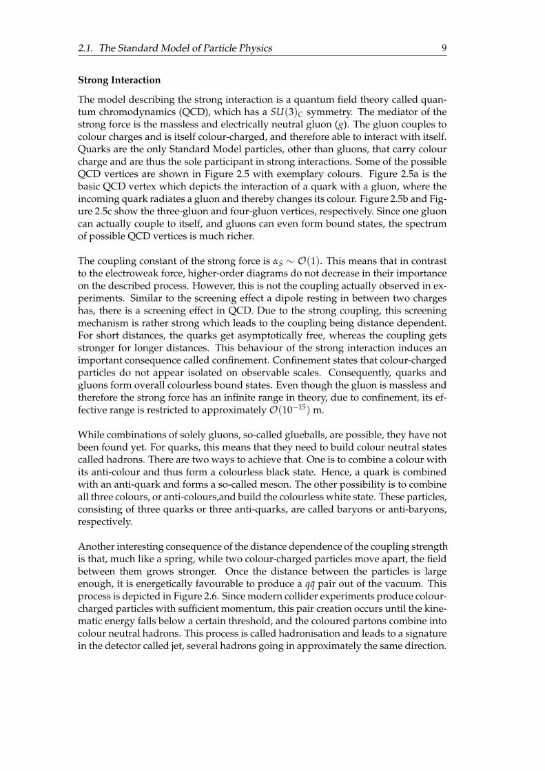
The model describing the strong interaction is a quantum field theory called quan-tum chromodynamics (QCD), which has a SU(3)C symmetry. The mediator of thestrong force is the massless and electrically neutral gluon (g). The gluon couples tocolour charges and is itself colour-charged, and therefore able to interact with itself.Quarks are the only Standard Model particles, other than gluons, that carry colourcharge and are thus the sole participant in strong interactions. Some of the possibleQCD vertices are shown in Figure 2.5 with exemplary colours. Figure 2.5a is thebasic QCD vertex which depicts the interaction of a quark with a gluon, where theincoming quark radiates a gluon and thereby changes its colour. Figure 2.5b and Fig-ure 2.5c show the three-gluon and four-gluon vertices, respectively. Since one gluoncan actually couple to itself, and gluons can even form bound states, the spectrumof possible QCD vertices is much richer.
The coupling constant of the strong force is αS ∼ O(1). This means that in contrastto the electroweak force, higher-order diagrams do not decrease in their importanceon the described process. However, this is not the coupling actually observed in ex-periments. Similar to the screening effect a dipole resting in between two chargeshas, there is a screening effect in QCD. Due to the strong coupling, this screeningmechanism is rather strong which leads to the coupling being distance dependent.For short distances, the quarks get asymptotically free, whereas the coupling getsstronger for longer distances. This behaviour of the strong interaction induces animportant consequence called confinement. Confinement states that colour-chargedparticles do not appear isolated on observable scales. Consequently, quarks andgluons form overall colourless bound states. Even though the gluon is massless andtherefore the strong force has an infinite range in theory, due to confinement, its ef-fective range is restricted to approximately O(10−15) m.
While combinations of solely gluons, so-called glueballs, are possible, they have notbeen found yet. For quarks, this means that they need to build colour neutral statescalled hadrons. There are two ways to achieve that. One is to combine a colour withits anti-colour and thus form a colourless black state. Hence, a quark is combinedwith an anti-quark and forms a so-called meson. The other possibility is to combineall three colours, or anti-colours,and build the colourless white state. These particles,consisting of three quarks or three anti-quarks, are called baryons or anti-baryons,respectively.
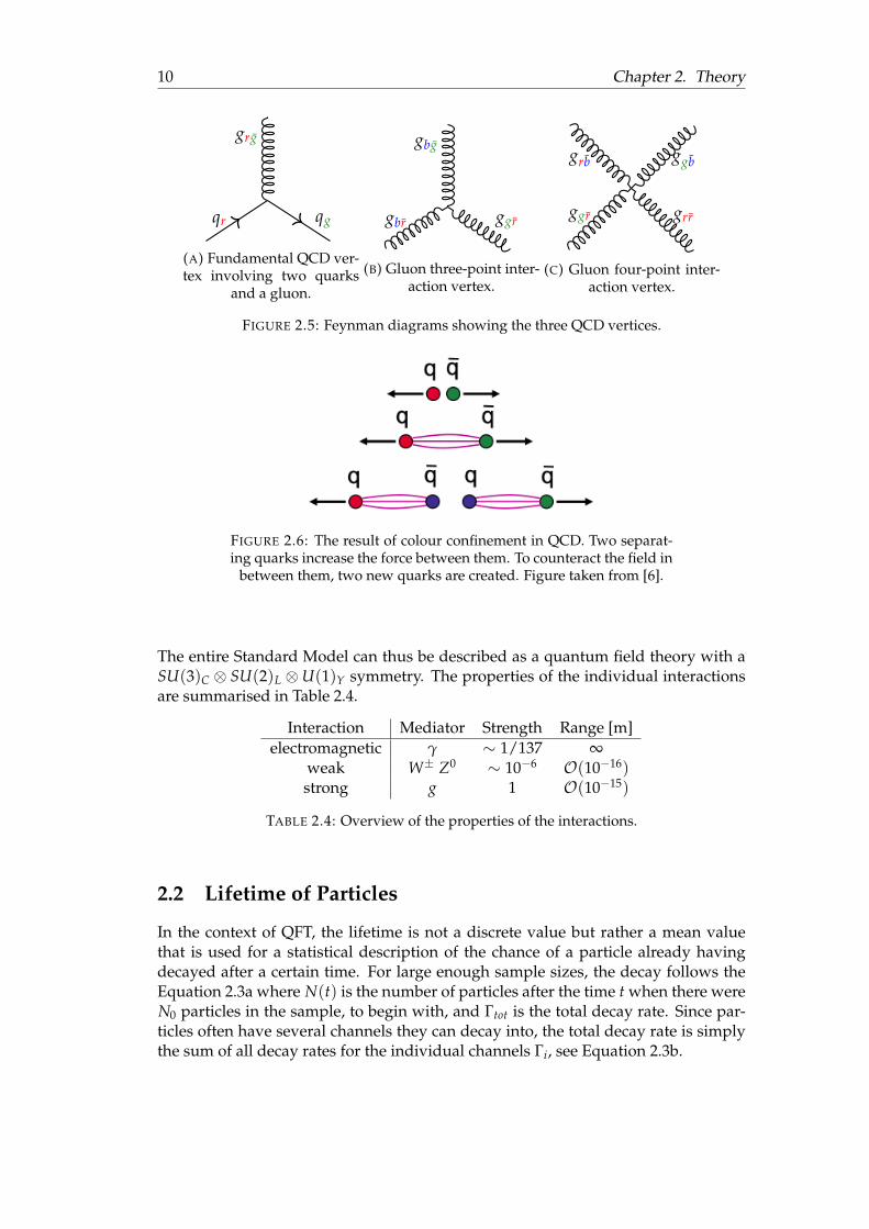
Another interesting consequence of the distance dependence of the coupling strengthis that, much like a spring, while two colour-charged particles move apart, the fieldbetween them grows stronger. Once the distance between the particles is largeenough, it is energetically favourable to produce a qq pair out of the vacuum. Thisprocess is depicted in Figure 2.6. Since modern collider experiments produce colour-charged particles with sufficient momentum, this pair creation occurs until the kine-matic energy falls below a certain threshold, and the coloured partons combine intocolour neutral hadrons. This process is called hadronisation and leads to a signaturein the detector called jet, several hadrons going in approximately the same direction.
10 Chapter 2. Theory
qr qg
grg
(A) Fundamental QCD ver-tex involving two quarks
and a gluon.
gbr ggr
gbg
(B) Gluon three-point inter-action vertex.
ggr
grb
grr
ggb
(C) Gluon four-point inter-action vertex.
FIGURE 2.5: Feynman diagrams showing the three QCD vertices.
FIGURE 2.6: The result of colour confinement in QCD. Two separat-ing quarks increase the force between them. To counteract the field in
between them, two new quarks are created. Figure taken from [6].
The entire Standard Model can thus be described as a quantum field theory with aSU(3)C ⊗ SU(2)L ⊗U(1)Y symmetry. The properties of the individual interactionsare summarised in Table 2.4.
Interaction Mediator Strength Range [m]electromagnetic γ ∼ 1/137 ∞
weak W± Z0 ∼ 10−6 O(10−16)strong g 1 O(10−15)
TABLE 2.4: Overview of the properties of the interactions.
2.2 Lifetime of Particles
In the context of QFT, the lifetime is not a discrete value but rather a mean valuethat is used for a statistical description of the chance of a particle already havingdecayed after a certain time. For large enough sample sizes, the decay follows theEquation 2.3a where N(t) is the number of particles after the time t when there wereN0 particles in the sample, to begin with, and Γtot is the total decay rate. Since par-ticles often have several channels they can decay into, the total decay rate is simplythe sum of all decay rates for the individual channels Γi, see Equation 2.3b.
2.2. Lifetime of Particles 11
N(T) = N0 · e−Γtott Γtot = ∑i
Γi τ =1
Γtot(2.3a-c)
Γ =(2π)4
2MS∫|M|2δ4
(P−
n
∑i=1
pi
)n
∏i=1
d3~pi
(2π)32Ei(2.4)
For every single decay channel, Γi can be calculated using Fermi’s Golden Rule,displayed in Equation 2.4. M and P are the mass and four-momentum of the decay-ing particle. pi and Ei are the four-momentum and energy of the decay products. S isa statistical factor accounting for identical particles. The absolute value of the matrixelement |M|, sometimes called amplitude, can be calculated using Feynman calcu-lus and includes all dynamical properties of the process. The δ-function ensures thatenergy- and momentum-conservation is upheld. As can be seen in Equation 2.3c thetotal decay rate is connected to the mean lifetime τ, which is the average the time ittakes for a particle to decay.
These dependencies on the lifetime τ lead to a couple of reasons for a long meanlifetime of a particle.
• Due to energy-conversation, particles are only able to decay into lighter par-ticles. Therefore, the lightest particle in a system including a conserved, oralmost conserved, quantum number has no possible decay mode that wouldnot violate the conserved quantity and thus a long τ. This can be seen for ex-ample with the proton (p). Protons are the lightest baryons and the baryonnumber is a conserved quantity. Consequently, a free proton has an extremelylong mean lifetime.6
• When the available phase space for the decay is limited, the integral in Equa-tion 2.4 leads to a small outcome. This happens when there is a slightly heavierparticle than the lightest particle of a system of an (almost) conserved quantumnumber. As an example serves the neutron which is the second lightest baryonand only a little heavier than its decay products p, e− and νe. The already ratherweak β-decay is further suppressed, which leads to a neutron lifetime of τn ≈880 seconds [8].
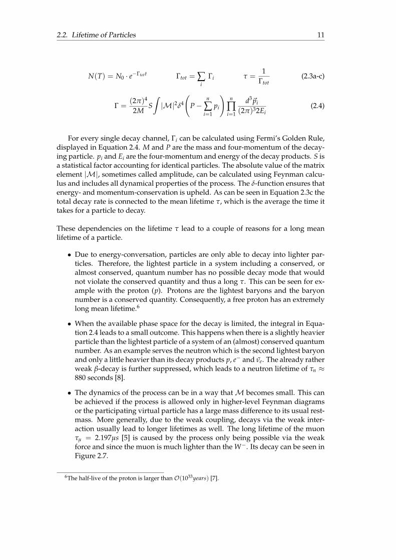
• The dynamics of the process can be in a way thatM becomes small. This canbe achieved if the process is allowed only in higher-level Feynman diagramsor the participating virtual particle has a large mass difference to its usual rest-mass. More generally, due to the weak coupling, decays via the weak inter-action usually lead to longer lifetimes as well. The long lifetime of the muonτµ = 2.197µs [5] is caused by the process only being possible via the weakforce and since the muon is much lighter than the W−. Its decay can be seen inFigure 2.7.
6The half-live of the proton is larger than O(1033years) [7].
12 Chapter 2. Theory
µ−
νµ
W−
e−
νe
FIGURE 2.7: Feynman diagram for the decay of the muon.
2.3 The need for New Physics
The Standard Model is one of the experimentally best tested and verified theoriesin physics and had tremendous success in many of its predictions. As examples forthis serve the prediction of the existence of the charm and top quarks [9, 10] and thebosons W±, Z0 and H0 [11, 12]. Nonetheless, there are open questions that cannotbe solved within the Standard Model, and therefore might need an extension of it oreven a new theory altogether. One of the instances that could be solved, through anextension of the Standard Model, was the observation of neutrino oscillations7 [13].Since neutrino oscillations are only possible if neutrinos possess mass and the Stan-dard Model considered them massless, the Standard Model needed to be extendedtowards massive neutrinos [4].
Unification of the Forces GUT
Since the electroweak unification already provided a mechanism that encloses thedescription of two fundamental interactions in one model, theorists believe thatthere could also be a theory combining the electromagnetic, weak and strong forceinto one model, called Grand Unified Theory (GUT). This is expected to happen atthe GUT scale at O(1016 GeV) [14], and would imply that the coupling constants ofthe electromagnetic, weak and strong interaction become similar at the GUT scale.As shown in Figure 2.8a extrapolations from the Standard Model to the GUT scaledo not yield that result. Therefore, new physics between the weak scale and the GUTscale is necessary for a possible unification, as sketched in Figure 2.8b.At the Planck scale O(1019 GeV) gravitational effects can no longer be neglected inparticle interactions and thus a full description would need to incorporate a quantum-mechanical description of gravity8. Therefore, opening the possibility for a furtherunification sometimes referred to as Theory of Everything.
Dark Matter
There are astrophysical observations, such as galactic rotation curves [17], stellar ve-locity dispersions [18], effects of gravitational lensing [19] or general cosmologicalmodels [20] which hint to the existence of large amounts of massive matter that doesnot interact electromagnetically or strongly and cannot be explained by the Stan-dard Model. Since this matter does not interact electromagnetically, it cannot be seenwith any sort of light and is therefore called dark matter. Recent measurements bythe Planck satellite [21] conclude that the matter composed by the Standard Model
7Takaaki Kajita and Arthur McDonald received the Nobel prize in 2015 for that discovery.8The current description of gravity, given by general relativity, seems to be fundamentally incom-
patible with the Standard Model [15].
2.3. The need for New Physics 13
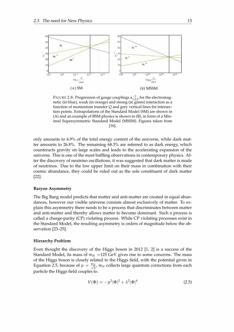
(A) SM (B) MSSM
FIGURE 2.8: Progression of gauge couplings α−11,2,3 for the electromag-
netic (in blue), weak (in orange) and strong (in green) interaction as afunction of momentum transfer Q and grey vertical lines for intersec-tion points. Extrapolations of the Standard Model (SM) are shown in(A) and an example of BSM physics is shown in (B), in form of a Min-imal Supersymmetric Standard Model (MSSM). Figures taken from
[16].
only amounts to 4.9% of the total energy content of the universe, while dark mat-ter amounts to 26.8%. The remaining 68.3% are referred to as dark energy, whichcounteracts gravity on large scales and leads to the accelerating expansion of theuniverse. This is one of the most baffling observations in contemporary physics. Af-ter the discovery of neutrino oscillations, it was suggested that dark matter is madeof neutrinos. Due to the low upper limit on their mass in combination with theircosmic abundance, they could be ruled out as the sole constituent of dark matter[22].
Baryon Asymmetry
The Big Bang model predicts that matter and anti-matter are created in equal abun-dances, however our visible universe consists almost exclusively of matter. To ex-plain this asymmetry there needs to be a process that discriminates between matterand anti-matter and thereby allows matter to become dominant. Such a process iscalled a charge-parity (CP) violating process. While CP violating processes exist inthe Standard Model, the resulting asymmetry is orders of magnitude below the ob-servation [23–25].
Hierarchy Problem
Even thought the discovery of the Higgs boson in 2012 [1, 2] is a success of theStandard Model, its mass of mH =125 GeV gives rise to some concerns. The massof the Higgs boson is closely related to the Higgs field, with the potential given inEquation 2.5, because of µ = mH√
2, mH collects large quantum corrections from each
particle the Higgs field couples to.
V(Φ) = −µ2|Φ|2 + λ2|Φ|4 (2.5)
14 Chapter 2. Theory
H0 λ f
f
H0
f
(A) Fermion interaction.
H0λS
S
H0
(B) Scalar boson interaction.
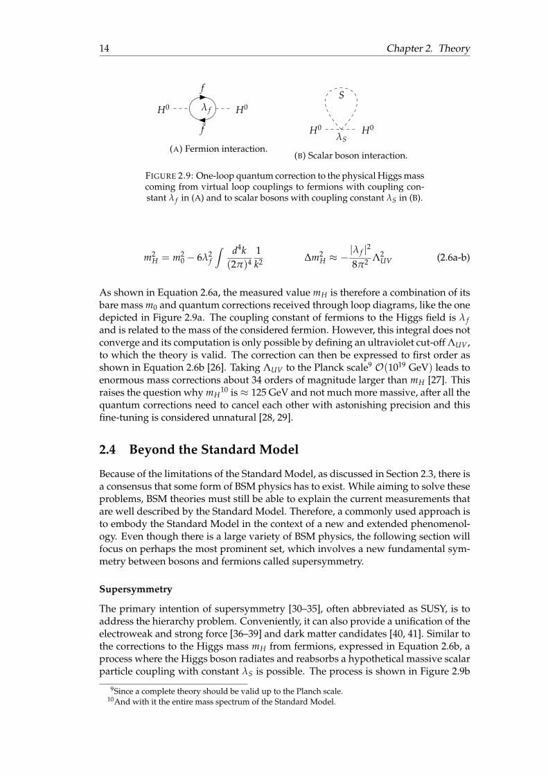
FIGURE 2.9: One-loop quantum correction to the physical Higgs masscoming from virtual loop couplings to fermions with coupling con-stant λ f in (A) and to scalar bosons with coupling constant λS in (B).
m2H = m2
0 − 6λ2f
∫ d4k(2π)4
1k2 ∆m2
H ≈ −|λ f |2
8π2 Λ2UV (2.6a-b)
As shown in Equation 2.6a, the measured value mH is therefore a combination of itsbare mass m0 and quantum corrections received through loop diagrams, like the onedepicted in Figure 2.9a. The coupling constant of fermions to the Higgs field is λ fand is related to the mass of the considered fermion. However, this integral does notconverge and its computation is only possible by defining an ultraviolet cut-off ΛUV ,to which the theory is valid. The correction can then be expressed to first order asshown in Equation 2.6b [26]. Taking ΛUV to the Planck scale9 O(1019 GeV) leads toenormous mass corrections about 34 orders of magnitude larger than mH [27]. Thisraises the question why mH
10 is≈ 125 GeV and not much more massive, after all thequantum corrections need to cancel each other with astonishing precision and thisfine-tuning is considered unnatural [28, 29].
2.4 Beyond the Standard Model
Because of the limitations of the Standard Model, as discussed in Section 2.3, there isa consensus that some form of BSM physics has to exist. While aiming to solve theseproblems, BSM theories must still be able to explain the current measurements thatare well described by the Standard Model. Therefore, a commonly used approach isto embody the Standard Model in the context of a new and extended phenomenol-ogy. Even though there is a large variety of BSM physics, the following section willfocus on perhaps the most prominent set, which involves a new fundamental sym-metry between bosons and fermions called supersymmetry.
Supersymmetry
The primary intention of supersymmetry [30–35], often abbreviated as SUSY, is toaddress the hierarchy problem. Conveniently, it can also provide a unification of theelectroweak and strong force [36–39] and dark matter candidates [40, 41]. Similar tothe corrections to the Higgs mass mH from fermions, expressed in Equation 2.6b, aprocess where the Higgs boson radiates and reabsorbs a hypothetical massive scalarparticle coupling with constant λS is possible. The process is shown in Figure 2.9b
9Since a complete theory should be valid up to the Planch scale.10And with it the entire mass spectrum of the Standard Model.
2.4. Beyond the Standard Model 15
and yields a correction term for mH, which is expressed to first order in Equation 2.7[42].
∆m2H ≈
|λS|216π2 [Λ
2UV − 2m2
S ln(ΛUV
mS)] (2.7)
When each fermion of the Standard Model is associated with two scalar bosons,where λS = |λ f |2, the Λ2
UV terms in Equations 2.6b and 2.7 cancel nicely. This leadsto the hypothesis that there is a new fundamental symmetry, called supersymmetry,which associates fermions to bosons and vice versa. The mathematical realisation ofthis is an operator Q that transforms fermionic states into bosonic ones and bosonicstates into fermionic ones, as expressed in Equation 2.8.
Q| f ermion〉 = |boson〉 Q|boson〉 = | f ermion〉 (2.8)
Further restrictions on the model can ensure that higher-order corrections also can-cel each other. Particles linked by Q are called superpartners and form so-calledsupermultiplets [43]. Besides the spin, they are equal in their quantum numbers.
To distinguish between Standard Model particles and their superpartners, the su-perpartners of the Standard Model particles are denoted with an additional tilde "~"above the particle symbol. For the superpartners of Standard Model particles thenaming convention is as follows: to represent their scalar nature, superpartners offermions acquire the prefix "s" and thus are called sfermions, while superpartnersof bosons pick up the suffix "ino". Therefore, the superpartners of gauge bosonsare referred to as gauginos. Since left-handed and right-handed particles are treateddifferently in the Standard Model, both of them get linked to their own supersym-metric partner. Due to the scalar nature of that superpartner, they are, however, nolonger left- and right-handed. This way there is at least one supersymmetric partnerfor each Standard Model particle. The entire set of supersymmetric partners of theStandard Model particles is often referred to as supersymmetric particles.
Since the term supersymmetry consolidates several different models, there are theo-ries with a much larger particle content. To avoid gauge anomalies, the models haveto add more particles than just the sfermions and gauginos [44]. The model withthe smallest amount of added particles, that avoids these gauge anomalies, is calledMinimal Supersymmetric (version of the) Standard Model (MSSM) and requires, inaddition to sfermions and gauginos, five Higgs bosons and their higgsinos insteadof the usual one [45]. In the MSSM the electroweak symmetry breaking, which givesthe W±- and Z0-bosons their masses, leads to a mixing of the gauginos with the hig-gsinos into mass eigenstates. The uncharged gauginos (B and W0) and higgsinos (H0
uand H0
d) build four neutral mass eigenstates, called neutralinos χ0i (i = 1, 2, 3, 4)11,
and the charged winos (W+ and W−) and higgsinos (H+u and H−d ) form four charged
eigenstates, called charginos χ±i (i = 1, 2)12 This mixing into new mass states also oc-curs for sfermions within one generation. For the first two generations this effect isnegligible and thus ignored, while the third generation mixes into the mass eigen-states ti, bi and τi (i = 1, 2). The entire additional particle content the MSSM predicts
11The convention is to order the labels by ascending mass, so that mχ01< mχ0
2< mχ0
3< mχ0
4.
12The convention is to order the labels by ascending mass, so that mχ±1< mχ±2
.
16 Chapter 2. Theory
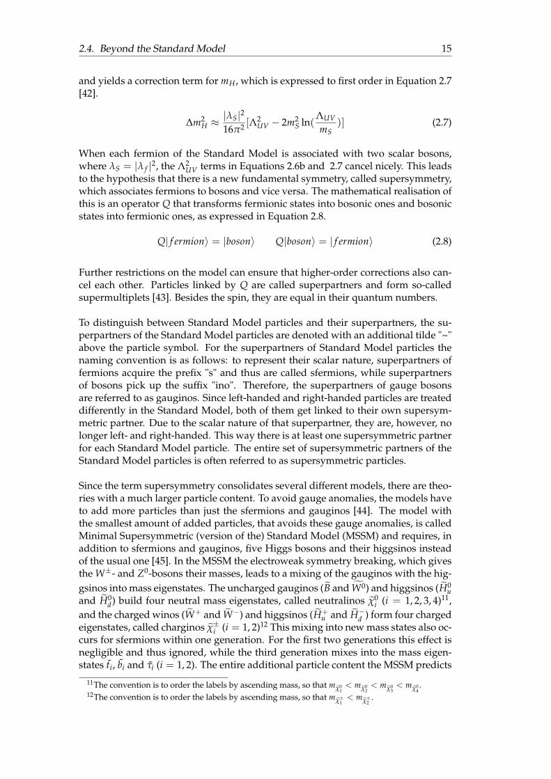
Name Spin PR Gauge Eigenstate Mass EigenstateHiggs Bosons 0 +1 H0
u H0d H+
u H−d h0 A0 H±
uL uR dL dR (same)Squarks 0 -1 sL sR cL cR (same)
tL tR bL bR t1 t2 b1 b1eL eR νe (same)
Sleptons 0 -1 µL µR νµ (same)τL τR ντ τ1 τ2 ντ
Gluino 1/2 -1 g (same)Neutralinos 1/2 -1 B0 W0 H0
u H0d χ0
1 χ02 χ0
3 χ04
Charginos 1/2 -1 W± H+u H−d χ±1 χ±2
Gravitiino 3/2 -1 G (same)
TABLE 2.5: Additional particles predicted by the Minimal Supersym-metric Standrad Model. Table taken from (Cite martin 19)
is shown in Table 2.5, including their spin, gauge eigenstates, mass eigenstates anda new property PR called R-parity.
R-parity
In order to explain the long lifetime of the proton, the Standard Model needs baryonnumber and lepton number conservation. However, many supersymmetric mod-els do violate these conservations if no further measures are taken. Therefore, theyoften introduce a new multiplicative quantum number called R-parity13, which isdefined in Equation 2.9 [46], where S is the spin, B the baryon number and L thelepton number of the particle.
PR = (−1)2S+3(B−L) (2.9)
All Standard Model particles and the added Higgs bosons have PR = +1 and theirsuperpartners have PR = −1. In order to prohibit the proton decay, R-parity is oftenconsidered to be a conserved quantity14 [48, 49], which has some notable implica-tions. Interactions between Standard Model particles can only lead to the productionof even numbers (mostly pairs) of supersymmetric particles. Furthermore, all super-symmetric particles have an odd amount of supersymmetric particles in their decayproducts and thus cannot decay into exclusively Standard Model particles. Fromthere follows, that the Lightest Supersymmetric Particle (LSP) cannot decay any fur-ther and therefore is stable. If it is electrically neutral and carries no colour charge, itcan function as a dark matter candidate. Many SUSY models keep the dark matterrequirements in mind and lead to the lightest neutralino or the gravitino15 being theLSP and thus a suitable dark matter candidate [50].
13Sometimes also referred to as matter parity.14It is also possible to build models that do not conserve R-parity and lead to protons lifetimes many
times larger than the age of the universe [47].15Supersymmetric partner of the graviton, the mediator of gravity in a GUT.
2.4. Beyond the Standard Model 17
Supersymmetry breaking
Supersymmetry has a noteworthy problem. If there where a perfect symmetry be-tween particles and their superpartners, all supersymmetric particles would notonly have the exact same quantum numbers, except the spin, but also exactly thesame mass, which means they would be already produced at contemporary exper-iments and thus would be observable. Since no supersymmetric particle has beenfound to this day, supersymmetry must be a broken symmetry so the superpartnerscan differ in mass. There are several ways to introduce this breaking mechanism andSUSY models are often distinguished by their breaking mechanism. Many modelsinclude a separation of the observable SUSY sector from a hidden SUSY-breakingsector, for example by assuming additional spacetime dimensions [51, 52]. Differenttypes of mediation between the visible and hidden sector lead to different modelslike gauge-mediated supersymmetry breaking (GMSB) [42, 53], anomaly-mediatedsupersymmetry breaking (AMSB) [54, 55] or minimal supergravity (mSUGRA) [56,57]. However, the expected mass scale of many of those models is on the order ofa few TeV and are therefore within the range of modern experiments [45, 58, 59].Since there was no sign of a supersymmetric particle so far, experiments set increas-ingly stronger exclusion limits on the masses of supersymmetric particles [60, 61].Thereby reducing the available phase space for supersymmetric particles substan-tially [62–64]. Unfortunately, with increasing mass difference between the StandardModel and supersymmetric particles the remaining possible models yield less pleas-ant solutions to the hierarchy problem [65].
Stable Massive Particles
Since many BSM theories want to have a dark matter candidate, and dark matter hasto be stable on the time scale of the universe16, many of them include Stable MassiveParticles (SMPs). In models with additional compactified dimensions for exampleStandard Model particles are accompanied by Kaluza-Klein excitations, which dif-fer in mass. A conserved symmetry leads to the lightest Kaluza-Klein particle beinglong-lived [66]. In supersymmetry many different models predict SMPs regardlessof whether they conserve R-parity [67, 68] or not [69, 70]. In models that conserveR-parity the LSP is often a suitable candidate for dark matter and thus electricallyneutral and colourless.
If the next-to-lightest supersymmetric particle is just slightly heavier than the LSP,it could be long-lived and traverse a particle detector and thus be considered sta-ble. When it is electrically charged or carries an additional colour charge, it wouldinteract with the detector and therefore would be detectable, see Section 3.2 andChapter 4. One possibly exploitable difference to Standard Model particles is theconsiderably larger mass, which would lead to them propagating the detector atconsiderably lower velocities. Therefore, their signature could look like the signa-ture of a much heavier and slower copy of a Standard Model particle. From theconsiderably slower velocity follows that searches for SMPs have a relatively smallbackground of Standard Model processes with similar signatures in the event. How-ever, detector effects do provide a background and therefore a good understandingof the detector itself is necessary before a search for charged stable massive particlescan be conducted.
16Otherwise it would decay and would not be as abundant in the universe.
18 Chapter 2. Theory
Depending on the exact breaking mechanism, the stau (τ), the lighter chargino (χ±1 )or gluinos (g) are possible candidates for charged stable massive particles in theMSSM. Similar to quarks, gluinos would hadronise into R-hadrons which wouldthen interact with the detector and could even undergo a process that changes theircharge. So far searches for SMPs remained unsuccessful but where able to placestringent limits on their minimal masses [71].
2.5 Summary
The Standard Model of particle physics describes elementary particles and three oftheir four know interactions. Even though it has been highly successful so far, it isincomplete and therefore physics beyond the Standard Model has to exist. One no-table class of theories extending the Standard Model is called supersymmetry, whichproposes a new fundamental symmetry between bosons and fermions. It predicts aset of new particles with similar quantum numbers, except for the spin. Due to thefact that such particles have not been found yet, the symmetry must be softly brokenand the supersymmetric particles must have masses considerably larger than theirStandard Model counterparts. Some of these models include charged stable mas-sive particles, which would register the same information in the detector as a muchheavier copy of the muon.
19
Chapter 3
The Experiment
This chapter focuses on the experimental setup. The Conseil Europeen pour laRecherche Nucleaire (CERN) is one of the worlds largest research centres. It is lo-cated at the Franco–Swiss border near Geneva and mainly focuses on research inparticle physics and hence operates different particle accelerators and hosts multipledetectors. CERN was founded in 1954 and was one of Europe’s first joint venturesin science. Today there are 23 member states [72, 73].At first, this chapter introduces the main experiment at CERN, the Large HadronCollider (LHC) [74], followed by a brief description of the ATLAS Experiment [75]with a focus on the detector components relevant to this work.
3.1 The Large Hadron Collider
Currently, the LHC is the largest and most powerful particle collider in the worldand is residing in the tunnel that was built for its predecessor, the Large ElectronPositron Collider (LEP) [76–78]. As the name suggests LEP used to accelerate andcollide electrons and positrons1 whereas the LHC works with hadrons. More pre-cisely, most of the time the LHC accelerates and collides protons2. During somespecial data-taking runs, called heavy-ion runs, the LHC also operates with lead-nuclei and produces proton–lead and lead–lead collisions [79]. This work uses datafrom pp collisions, therefore the following explanations focus on the proton–protonruns of the LHC. Since the synchrotron-radiation scales with the mass of the ac-celerated particle according to m−4 [80], hadron colliders can achieve much higherenergies than electron–positron colliders could. This advantage in energy comes ata cost. While electrons and positrons are considered to be fundamental particles andtherefore without substructure, hadrons do have substructure, their constituents arereferred to as partons (quarks or gluons). From this follows, that the momenta of theinteracting partons in hadron collisions are not known exactly, but rather describedstatistically by a distribution called parton distribution function (PDF). Furthermore,it is not clear which parton took part in the interaction or whether or not several par-tons of the same hadron took part in an interaction.
The tunnel of the LHC is located between 175 m (under the Jura) and 50 m (closeto Lake Geneva) below the surface, resulting in a tilt of roughly 1,4%. The LHC’sshape roughly describes a circle with a circumference of 26.659 km that is composedof eight arcs and eight straight sections. In order to bend the two particle beamsalong the arcs, a total of 1232 dipole magnets are used and 392 quadupole magnets
1Anti-electrons.2A baryon build out of two up quarks and one down quark.
20 Chapter 3. The Experiment
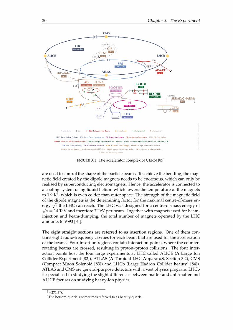
FIGURE 3.1: The accelerator complex of CERN [85].
are used to control the shape of the particle beams. To achieve the bending, the mag-netic field created by the dipole magnets needs to be enormous, which can only berealised by superconducting electromagnets. Hence, the accelerator is connected toa cooling system using liquid helium which lowers the temperature of the magnetsto 1.9 K3, which is even colder than outer space. The strength of the magnetic fieldof the dipole magnets is the determining factor for the maximal centre-of-mass en-ergy
√s the LHC can reach. The LHC was designed for a centre-of-mass energy of√
s = 14 TeV and therefore 7 TeV per beam. Together with magnets used for beam-injection and beam-dumping, the total number of magnets operated by the LHCamounts to 9593 [81].
The eight straight sections are referred to as insertion regions. One of them con-tains eight radio-frequency cavities for each beam that are used for the accelerationof the beams. Four insertion regions contain interaction points, where the counter-rotating beams are crossed, resulting in proton–proton collisions. The four inter-action points host the four large experiments at LHC called ALICE (A Large IonCollider Experiment [82]), ATLAS (A Toroidal LHC ApparatuS, Section 3.2), CMS(Compact Muon Solenoid [83]) and LHCb (Large Hadron Collider beauty4 [84]).ATLAS and CMS are general-purpose detectors with a vast physics program, LHCbis specialised in studying the slight differences between matter and anti-matter andALICE focuses on studying heavy-ion physics.
3−271.3◦C4The bottom-quark is sometimes referred to as beauty-quark.
3.1. The Large Hadron Collider 21
Before the protons can be injected into the LHC they have to go through an injectorchain, which subsequently increases the energy of the proton–beam. A schematicdrawing of the full CERN accelerator complex is shown in Figure 3.1. As protonsource, a bottle of hydrogen gas is used. After the electric field stripped the hydrogenatoms of their electrons, the remaining protons are accelerated to 50 MeV by a linearaccelerator (Linac 2). Subsequently, the protons are injected into the Proton Syn-chrotron Booster (PSB), which brings them to 1.4 GeV. The Proton Synchrotron (PS)further increases their energy to 25 GeV. The Last stop, before entering the LHC, isthe Super Proton Synchrotron (SPS) where the protons reach 450 GeV. From the SPSthe protons are injected into the two beam pipes of the LHC, while being separatedinto 2808 different packages, called bunches, of approximately 1.2 · 1011 protons witha time spacing of 25 ns5 [81, 86]. The LHC is responsible for the acceleration to thefinal collision energy. During the first period of data taking, Run–1, the LHC oper-ated at beam energies of 3.5 TeV(2010 and 2011) and 4 TeV (2012), which resultedin centre-of-mass energies of 7 TeV and 8 TeV, respectively [87]. After a two yearperiod without data taking, used for upgrades and maintenance, the LHC resumedits operation in 2015 with a centre of mass energy of 13 TeV for the whole Run–2 thatended in 2018 [88].
As expressed in Equation 3.1a the rate of a process dndt and its cross-section σ are
related by a quantity called instantaneous luminosity L. L itself depends on manyparameters of the accelerator and with the assumption of Gaussian shaped bunches,can be expressed as shown in Equation 3.1b. Where σx and σy are the widths in x-and y-direction of the Gauss shaped bunches, which revolve around the acceleratorring with frequency f . Nb is the number of bunches filled into each beam pipe andN1 and N2 are the amount of protons in each bunch. The LHC was designed withan instantaneous luminosity of 1034 cm−2s−1 in mind [75] and by the end of 2017actually managed to reach 2.06 · 1034 cm−2s−1 being twice its nominal value [89].In order to go from the rate dn
dt of a process to the total number of events during aspecific data-taking run, one has to integrate over time. Therefore, the integrated lu-minosity, given in Equation 3.1c, serves as a measure of how much data was taken.The total amount of events Ni of a specific process i is described by Equation 3.1d.
dndt
= L · σ L =Nb f N1N2
4πσxσyL =
∫Ldt Ni = σi · L (3.1a-d)
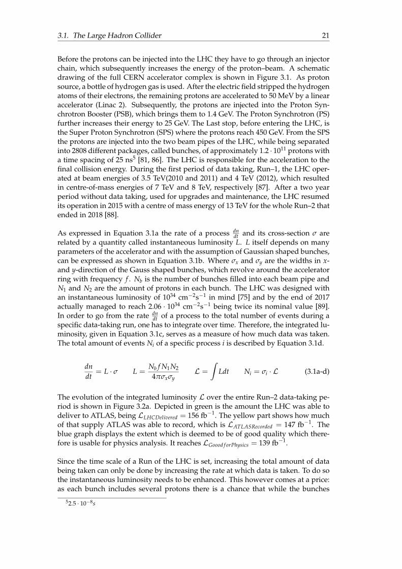
The evolution of the integrated luminosity L over the entire Run–2 data-taking pe-riod is shown in Figure 3.2a. Depicted in green is the amount the LHC was able todeliver to ATLAS, being LLHCDelivered = 156 fb−1. The yellow part shows how muchof that supply ATLAS was able to record, which is LATLASRecorded = 147 fb−1. Theblue graph displays the extent which is deemed to be of good quality which there-fore is usable for physics analysis. It reaches LGoood f orPhysics = 139 fb−1.
Since the time scale of a Run of the LHC is set, increasing the total amount of databeing taken can only be done by increasing the rate at which data is taken. To do sothe instantaneous luminosity needs to be enhanced. This however comes at a price:as each bunch includes several protons there is a chance that while the bunches
52.5 · 10−8s
22 Chapter 3. The Experiment
Month in YearJan '15
Jul '15Jan '16
Jul '16Jan '17
Jul '17Jan '18
Jul '18
-1fb
Tot
al In
tegr
ated
Lum
inos
ity
0
20
40
60
80
100
120
140
160ATLASPreliminary
LHC Delivered
ATLAS Recorded
Good for Physics
= 13 TeVs
-1 fbDelivered: 156-1 fbRecorded: 147
-1 fbPhysics: 139
2/19 calibration
(A) Integrated Luminosity. L
0 10 20 30 40 50 60 70 80
Mean Number of Interactions per Crossing
0
100
200
300
400
500
600
/0.1
]-1
Rec
orde
d Lu
min
osity
[pb
Online, 13 TeVATLAS -1Ldt=146.9 fb∫> = 13.4µ2015: <> = 25.1µ2016: <> = 37.8µ2017: <> = 36.1µ2018: <> = 33.7µTotal: <
2/19 calibration
(B) Pileup profile in ATLAS.
FIGURE 3.2: The integrated luminosity L delivered by the LHC dur-ing Run–2 pp data-taking is shown in (A) and the pile-up profile dur-
ing that period is shown in (B). Figures are taken from [90]
cross, several proton pairs collide and interact simultaneously. These additional in-teractions are referred to as pile-up and pose a challenge for the separation of eachinteraction and accordingly the reconstruction of the event. Figure 3.2b shows thepile-up profile for the recorded luminosity during Run–2, both separated for eachyear and combined. During the whole Run–2 an average of 〈µ〉 = 33.7 simultaneousinteractions were recorded in ATLAS, with values reaching up to 70 interactions atonce.
3.2 The ATLAS Detector
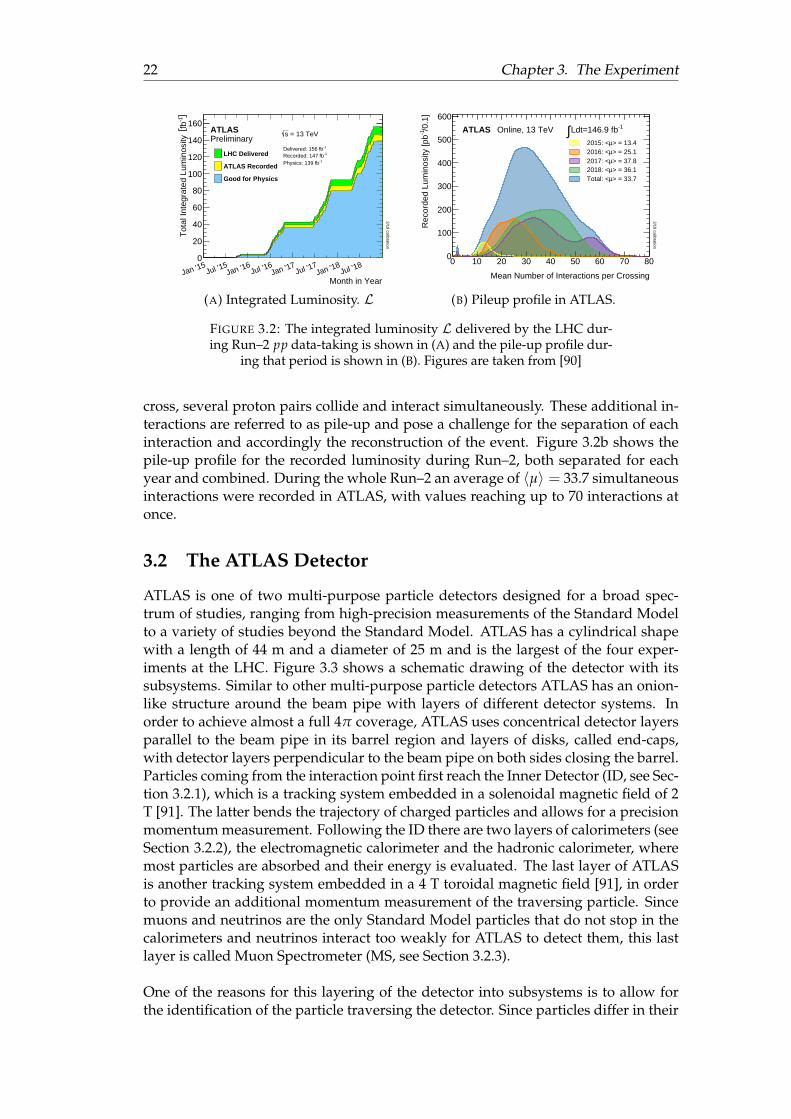
ATLAS is one of two multi-purpose particle detectors designed for a broad spec-trum of studies, ranging from high-precision measurements of the Standard Modelto a variety of studies beyond the Standard Model. ATLAS has a cylindrical shapewith a length of 44 m and a diameter of 25 m and is the largest of the four exper-iments at the LHC. Figure 3.3 shows a schematic drawing of the detector with itssubsystems. Similar to other multi-purpose particle detectors ATLAS has an onion-like structure around the beam pipe with layers of different detector systems. Inorder to achieve almost a full 4π coverage, ATLAS uses concentrical detector layersparallel to the beam pipe in its barrel region and layers of disks, called end-caps,with detector layers perpendicular to the beam pipe on both sides closing the barrel.Particles coming from the interaction point first reach the Inner Detector (ID, see Sec-tion 3.2.1), which is a tracking system embedded in a solenoidal magnetic field of 2T [91]. The latter bends the trajectory of charged particles and allows for a precisionmomentum measurement. Following the ID there are two layers of calorimeters (seeSection 3.2.2), the electromagnetic calorimeter and the hadronic calorimeter, wheremost particles are absorbed and their energy is evaluated. The last layer of ATLASis another tracking system embedded in a 4 T toroidal magnetic field [91], in orderto provide an additional momentum measurement of the traversing particle. Sincemuons and neutrinos are the only Standard Model particles that do not stop in thecalorimeters and neutrinos interact too weakly for ATLAS to detect them, this lastlayer is called Muon Spectrometer (MS, see Section 3.2.3).
One of the reasons for this layering of the detector into subsystems is to allow forthe identification of the particle traversing the detector. Since particles differ in their
3.2. The ATLAS Detector 23
FIGURE 3.3: Computer-generated schematic drawing of the ATLASdetector with its subsystems labelled and two humans in proportion.
Figure taken from [75].
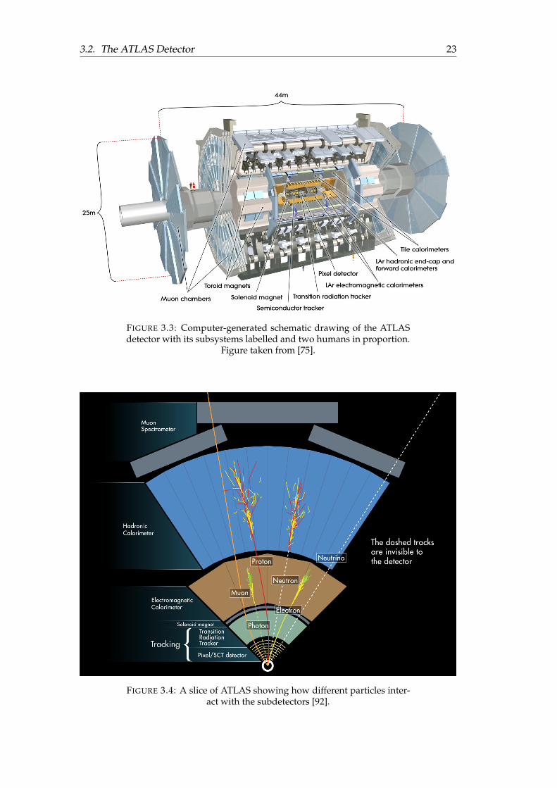
FIGURE 3.4: A slice of ATLAS showing how different particles inter-act with the subdetectors [92].
24 Chapter 3. The Experiment
(A) (B)
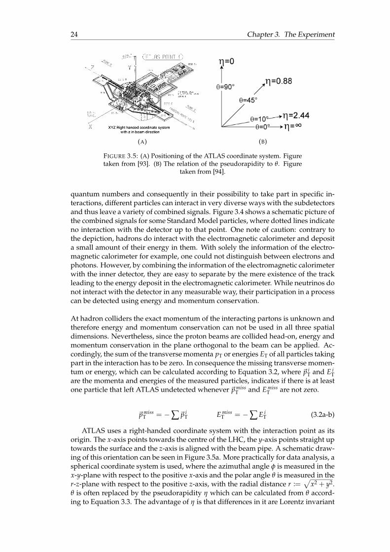
FIGURE 3.5: (A) Positioning of the ATLAS coordinate system. Figuretaken from [93]. (B) The relation of the pseudorapidity to θ. Figure
taken from [94].
quantum numbers and consequently in their possibility to take part in specific in-teractions, different particles can interact in very diverse ways with the subdetectorsand thus leave a variety of combined signals. Figure 3.4 shows a schematic picture ofthe combined signals for some Standard Model particles, where dotted lines indicateno interaction with the detector up to that point. One note of caution: contrary tothe depiction, hadrons do interact with the electromagnetic calorimeter and deposita small amount of their energy in them. With solely the information of the electro-magnetic calorimeter for example, one could not distinguish between electrons andphotons. However, by combining the information of the electromagnetic calorimeterwith the inner detector, they are easy to separate by the mere existence of the trackleading to the energy deposit in the electromagnetic calorimeter. While neutrinos donot interact with the detector in any measurable way, their participation in a processcan be detected using energy and momentum conservation.
At hadron colliders the exact momentum of the interacting partons is unknown andtherefore energy and momentum conservation can not be used in all three spatialdimensions. Nevertheless, since the proton beams are collided head-on, energy andmomentum conservation in the plane orthogonal to the beam can be applied. Ac-cordingly, the sum of the transverse momenta pT or energies ET of all particles takingpart in the interaction has to be zero. In consequence the missing transverse momen-tum or energy, which can be calculated according to Equation 3.2, where ~p i
T and E iT
are the momenta and energies of the measured particles, indicates if there is at leastone particle that left ATLAS undetected whenever ~p miss
T and E missT are not zero.
~p missT = −∑~p i
T E missT = −∑ E i
T (3.2a-b)
ATLAS uses a right-handed coordinate system with the interaction point as itsorigin. The x-axis points towards the centre of the LHC, the y-axis points straight uptowards the surface and the z-axis is aligned with the beam pipe. A schematic draw-ing of this orientation can be seen in Figure 3.5a. More practically for data analysis, aspherical coordinate system is used, where the azimuthal angle φ is measured in thex-y-plane with respect to the positive x-axis and the polar angle θ is measured in ther-z-plane with respect to the positive z-axis, with the radial distance r :=
√x2 + y2.
θ is often replaced by the pseudorapidity η which can be calculated from θ accord-ing to Equation 3.3. The advantage of η is that differences in it are Lorentz invariant
3.2. The ATLAS Detector 25
(A) (B)
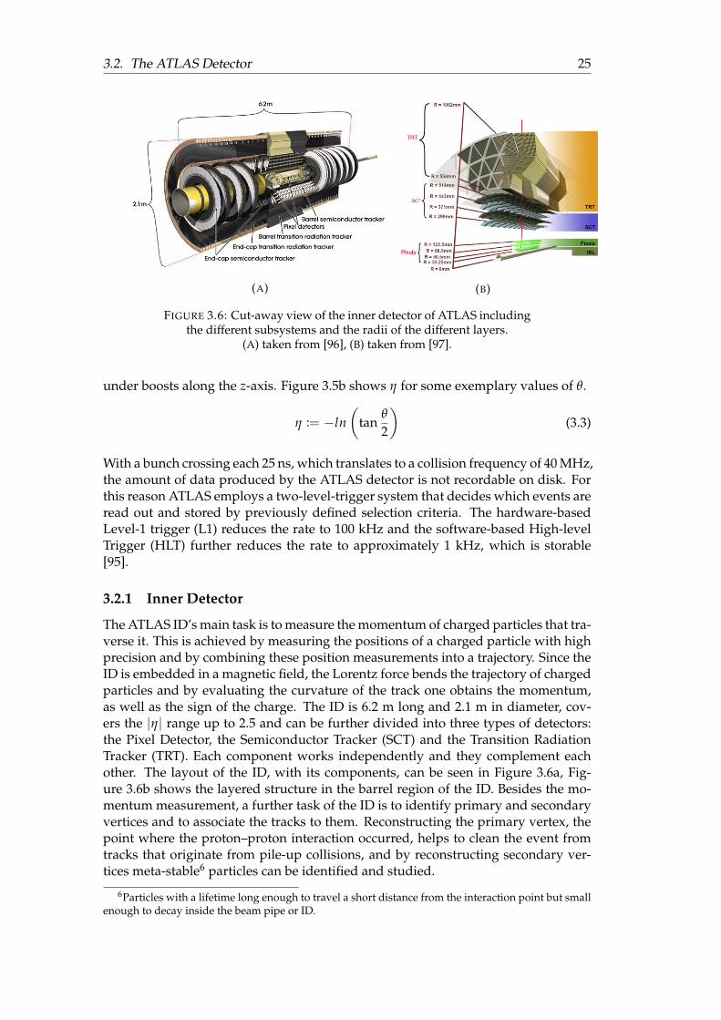
FIGURE 3.6: Cut-away view of the inner detector of ATLAS includingthe different subsystems and the radii of the different layers.
(A) taken from [96], (B) taken from [97].
under boosts along the z-axis. Figure 3.5b shows η for some exemplary values of θ.
η := −ln(
tanθ
2
)(3.3)
With a bunch crossing each 25 ns, which translates to a collision frequency of 40 MHz,the amount of data produced by the ATLAS detector is not recordable on disk. Forthis reason ATLAS employs a two-level-trigger system that decides which events areread out and stored by previously defined selection criteria. The hardware-basedLevel-1 trigger (L1) reduces the rate to 100 kHz and the software-based High-levelTrigger (HLT) further reduces the rate to approximately 1 kHz, which is storable[95].
3.2.1 Inner Detector
The ATLAS ID’s main task is to measure the momentum of charged particles that tra-verse it. This is achieved by measuring the positions of a charged particle with highprecision and by combining these position measurements into a trajectory. Since theID is embedded in a magnetic field, the Lorentz force bends the trajectory of chargedparticles and by evaluating the curvature of the track one obtains the momentum,as well as the sign of the charge. The ID is 6.2 m long and 2.1 m in diameter, cov-ers the |η| range up to 2.5 and can be further divided into three types of detectors:the Pixel Detector, the Semiconductor Tracker (SCT) and the Transition RadiationTracker (TRT). Each component works independently and they complement eachother. The layout of the ID, with its components, can be seen in Figure 3.6a, Fig-ure 3.6b shows the layered structure in the barrel region of the ID. Besides the mo-mentum measurement, a further task of the ID is to identify primary and secondaryvertices and to associate the tracks to them. Reconstructing the primary vertex, thepoint where the proton–proton interaction occurred, helps to clean the event fromtracks that originate from pile-up collisions, and by reconstructing secondary ver-tices meta-stable6 particles can be identified and studied.
6Particles with a lifetime long enough to travel a short distance from the interaction point but smallenough to decay inside the beam pipe or ID.
26 Chapter 3. The Experiment
Pixel Detector
The innermost sub-detector of the ID is the silicon Pixel Detector [98]. In the barrelregion, it consists of four concentric layers at average radii of 33.25 mm, 50.5 mm,88.5 mm and 122.5 mm and covers |η| values up to 1.7. The first layer, called In-sertable B-Layer (IBL [99]), was not part of the initial design of the Pixel Detectorbut could be added in 2014 after a narrower beam-pipe was installed. Due to its in-stallation at a very small radius, it was able to improve the identification of verticesproviding another high-precision hit improving the tracking. The typical pixel usedin the IBL has a size of 50 µm × 250 µm in transverse and longitudinal directionand a thickness of 200 µm. Pixels in the other three layers have a typical size of 50µm × 400 µm with a thickness of 250 µm. The barrel reaches a position resolutionaccuracy of 10 µm in φ and 115 µm in z. The end-cap consists of three disks on eachside, perpendicular to the beam-pipe at |z| values of 495 mm, 580 mm and 650 mmand covers the region 1.7 < |η| < 2.5. In total, the Pixel Detector consists of 86.4 · 106
pixels, 73.2 · 106 of them in the barrel and the remaining 13.2 · 106 in the end caps.In addition to the precision position information, the Pixel Detector is capable ofmeasuring the charge collected via a time-over-threshold measurement [100], whichserves as a value for the energy deposit in the Pixel Detector.
Semiconductor Tracker
The ATLAS ID’s second layer is the SCT [101]. The SCT is another silicon-baseddetector organised in four cylindrical double layers of silicon strip detectors withaverage radii between 299 mm and 514 mm, covering |η| values up to 1.4 in thebarrel region. The typical strip length is 126 mm with a pitch of 80 µm and the layersare mounted with a small stereo angle of 40 mrad in order to get information in thenon-precision direction along the strips (z-direction). The SCT achieves a resolutionof 16 µm in φ and 580 µm along the z-axis. The end-caps of the SCT consist of ninedisks on each side covering |η| values up to 2.5. In total, the SCT possesses 6.4 · 106
readout channels.
Transition Radiation Tracker
The TRT [102] is the last and outermost part of the ATLAS ID. Similar to the othertwo sub-detectors of the ID it consists of a barrel region and end-caps. The TRT ismade of thin-walled proportional drift tubes, called straw tubes. Each tube has adiameter of 4 mm and can detect radiation produced by relativistic particles travers-ing the polypropylene foils around the straws. Each straw is filled with gas7 and hasa gold-plated tungsten wire with a diameter of 30 µm in its centre, acting as an an-ode. In the barrel region, the TRT is composed of 52,544 straw tubes located outsidethe SCT, covering radii from 554 mm to 1082 mm. Each straw has a length of 144cm and is oriented parallel to the beam-pipe, covering |η| values up to 0.7. In bothend-capes 122,880 straws with a length of 37 cm, oriented radially to the beam-pipe,are used, which extend the covered |η| range to 2.0. In the barrel, the straws aresplit and read out from both sides, while the straws in the end-caps are red out onone side. Each channel provides a spatial resolution of 170 µm perpendicular to thedirection of the straw. Alongside the straw (z-direction in the barrel, r direction inthe end-caps) no measurement can be conducted. Since the strength of the transitionradiation depends on the velocity of the particle, the TRT allows for limited particle
770%Xe, 27%CO2, 3%O2, in leaking straws Argon was used as a substitute for the expensive Xenon.
3.2. The ATLAS Detector 27
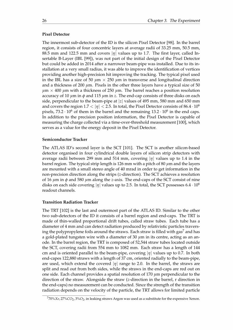
FIGURE 3.7: Schematic cut-away view of the calorimeter system ofATLAS and its positioning outside the inner detector, depicted in grey
right next to the beam-pipe. Figure taken from [105].
identification and is able to distinguish between light electrons and heavy chargedhadrons.
3.2.2 Calorimeters
The main goal of the ATLAS calorimeter system [103, 104] is to measure the energy aparticle loses by passing through the detector. Usually, calorimeters are designed ina way that the particle deposits its entire energy in them and is stopped. ATLAS usessampling calorimeters which are composed of passive and active materials placed ina sandwich structure. Inside of the passive material the traversing particle interactsintensively with the detector material and forms showers which are then absorbedby the active material, where the energy deposit is measured. This intensive interac-tion can either be achieved electromagnetically or via the strong interaction and thusform electromagnetic or hadronic showers, respectively. ATLAS uses both types ofshowers to measure the energy of a particle. The lighter particles, like electronsand the massless photons, are stopped in the electromagnetic calorimeter and theheavier hadrons are usually stopped in the hadronic calorimeter. Figure 3.7 shows aschematic drawing of the calorimeter system deployed in ATLAS.
Electromagnetic Calorimeter
When a highly energetic electron traverses the dense passive layers of the electro-magnetic calorimeter it is subject to bremsstrahlung and therefore emits a photon.In the presence of heavy nuclei, photons with a high-enough energy undergo a pair–creation process of electron–positron pairs. The combination of these two processesleads to the formation of electromagnetic showers. The showers die out when theenergy of the produced particles falls below a critical threshold at which ionisation
28 Chapter 3. The Experiment
energy loss takes over for electrons. The total charge produced in such a shower-ing process is proportional to the energy of the initial particle. By measuring thecharge in the active material the calorimeter can thereby estimate the total energybeing deposited. The radiation length resembles the distance where the energy hasbeen reduced to 1/e. Since ATLAS aims to measure the full energy, even for highlyenergetic electrons or photons, the electromagnetic calorimeter of ATLAS has a min-imum thickness of 22 radiation lengths [103]. Similar to the sub-detectors of the IDthe electromagnetic calorimeter consists of a barrel region covering a |η|-range upto 1.475, with a radial extension from approximately 1.4 m to 2.0 m and end-capsthat extend the range to 1.375 < |η| < 3.2. The passive material used is lead andthe active material employed is liquid argon8. The layers have an accordion-shapedstructure which allows for a design without holes in φ-direction. The resolutionvaries with η and reaches a granularity of ∆η × ∆φ = 0.025× 0.0245 in the barreland ∆η × ∆φ = 0.1× 0.1 in the end-caps. Since the particles reaching the electro-magnetic calorimeter have already traversed the inner detector, the cryostat and thesolenoid magnet and lost some energy doing so, a presampler was installed covering|η| < 1.8 to aid in the correction process for this energy loss.
Hadronic Calorimeter
Analogous to electrons, highly-energetic hadrons create particle showers when theytraverse dense material. The processes creating these showers however are differ-ent and caused by the strong interaction. While the showering mechanism is morecomplicated than the one for electromagnetic showers, the principle is similar. Thehadronic shower typically has a longer penetration depth though. Hence, an addi-tional and more dense hadronic calorimeter is used by ATLAS. Similar to the electro-magnetic shower, the depth of a hadronic shower is characterised by the hadronicinteraction length. The maximum thickness of the hadronic calorimeter is eleventimes the interaction length, which is enough to prevent a punch-through into theMuon Spectrometer. The barrel region consists of a barrel segment covering |η| < 1.0and an extended barrel with 0.8 < |η| < 1.7. The active layers are made of scintillatingtiles9 and the passive layers consist of iron. The granularity of the barrel region is∆η×∆φ = 0.1× 0.1 [104]. In the end-caps the hadronic calorimeter achieves a gran-ularity of ∆η × ∆φ = 0.2× 0.2 with liquid argon being used as active and lead aspassive material. In order to cover an additional |η| range of 3.1 < |η| < 4.9 ATLASadditionally employs a forward calorimeter using liquid argon as active material.The first layer of passive material is made of copper and the following two layersconsist of tungsten. With a radial extension of up to 4.2 m, the tile calorimeter canalso be used for time-of-flight measurements and calculations of the velocity of thetraversing particle.
3.2.3 Muon Spectrometer
The outermost component of ATLAS is the Muon Spectrometer, which serves twotasks: firstly, providing fast signals of traversing muons10 that the trigger systemcan use and secondly making a high precision measurement of the momentum oftraversing particles. Similar to the ID the MS, therefore, is immersed in a strongmagnetic field provided by eight toroid magnet coils and two end cap toroids with
8Therefore, the electromagnetic is often replaced with "Liquid Argon" or just LAr.9It is therefore often referred to as tile calorimeter.
10The only detectable Standard Model particle reaching the MS.
3.2. The ATLAS Detector 29
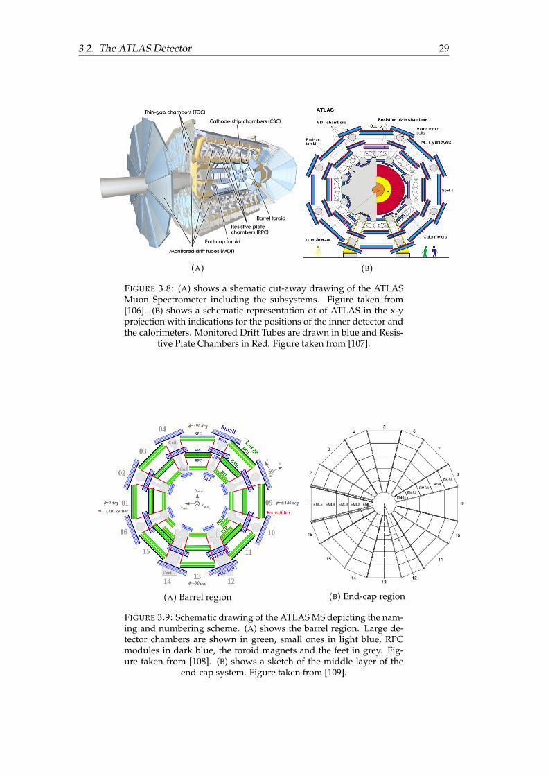
(A) (B)
FIGURE 3.8: (A) shows a shematic cut-away drawing of the ATLASMuon Spectrometer including the subsystems. Figure taken from[106]. (B) shows a schematic representation of of ATLAS in the x-yprojection with indications for the positions of the inner detector andthe calorimeters. Monitored Drift Tubes are drawn in blue and Resis-
tive Plate Chambers in Red. Figure taken from [107].
(A) Barrel region (B) End-cap region
FIGURE 3.9: Schematic drawing of the ATLAS MS depicting the nam-ing and numbering scheme. (A) shows the barrel region. Large de-tector chambers are shown in green, small ones in light blue, RPCmodules in dark blue, the toroid magnets and the feet in grey. Fig-ure taken from [108]. (B) shows a sketch of the middle layer of the
end-cap system. Figure taken from [109].
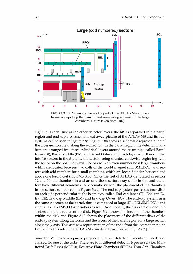
30 Chapter 3. The Experiment
FIGURE 3.10: Schematic view of a part of the ATLAS Muon Spec-trometer depicting the naming and numbering scheme for the large
chambers. Figure taken from [109].
eight coils each. Just as the other detector layers, the MS is separated into a barrelregion and end-caps. A schematic cut-away picture of the ATLAS MS and its sub-systems can be seen in Figure 3.8a, Figure 3.8b shows a schematic representation ofthe cross-section view along the z-direction. In the barrel region, the detector cham-bers are arranged into three cylindrical layers around the beam-pipe called BarrelInner (BI), Barrel Middle (BM) and Barrel Outer (BO). Each layer is further dividedinto 16 sectors in the φ-plane, the sectors being counted clockwise beginning withthe sector on the positive x-axis. Sectors with an even number host large chambers,which are located between two coils of the toroid magnet (BIL,BML,BOL) and sec-tors with odd numbers host small chambers, which are located under, between andabove one toroid coil (BIS,BMS,BOS). Since the feet of ATLAS are located in sectors12 and 14, the chambers in and around those sectors may differ in size and there-fore have different acronyms. A schematic view of the placement of the chambersin the sectors can be seen in Figure 3.9a. The end-cap system possesses four discson each side perpendicular to the beam axis, called End-cap Inner (EI), End-cap Ex-tra (EE), End-cap Middle (EM) and End-cap Outer (EO). The end-cap system usesthe same φ sectors as the barrel, thus is composed of large (EIL,EEL,EML,EOL) andsmall (EIS,EES,EMS,EOS) chambers as well. Additionally, the disks are divided intosectors along the radius of the disk. Figure 3.9b shows the location of the chamberswithin the disk and Figure 3.10 shows the placement of the different disks of theend-cap system along the z-axis and the layers of the barrel region for a large sectionalong the y-axis. This acts as a representation of the radii from the interaction point.Employing this setup the ATLAS MS can detect particles with |η| < 2.7 [110].
Since the MS has two separate purposes, different detector elements are used, spe-cialised for one of the tasks. There are four different detector types in service: Mon-itored Drift Tubes (MDT’s), Resistive Plate Chambers (RPC’s), Thin Gap Chambers
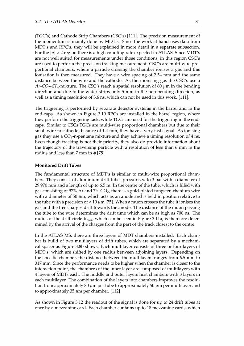
3.2. The ATLAS Detector 31
(TGC’s) and Cathode Strip Chambers (CSC’s) [111]. The precision measurement ofthe momentum is mainly done by MDT’s. Since the work at hand uses data fromMDT’s and RPC’s, they will be explained in more detail in a separate subsection.For the |η| > 2 region there is a high counting rate expected in ATLAS. Since MDT’sare not well suited for measurements under those conditions, in this region CSC’sare used to perform the precision tracking measurement. CSC’s are multi-wire pro-portional chambers, where a particle crossing the chamber ionises a gas and thisionisation is then measured. They have a wire spacing of 2.54 mm and the samedistance between the wire and the cathode. As their ionising gas the CSC’s use aAr-CO2-CF4-mixture. The CSC’s reach a spatial resolution of 60 µm in the bendingdirection and due to the wider strips only 5 mm in the non-bending direction, aswell as a timing resolution of 3.6 ns, which can not be used in this work. [111].
The triggering is performed by separate detector systems in the barrel and in theend-caps. As shown in Figure 3.10 RPCs are installed in the barrel region, wherethey perform the triggering task, while TGCs are used for the triggering in the end-caps. Similar to CSCs TGCs are multi-wire proportional chambers but due to theirsmall wire-to-cathode distance of 1.4 mm, they have a very fast signal. As ionisinggas they use a CO2-n-pentane mixture and they achieve a timing resolution of 4 ns.Even though tracking is not their priority, they also do provide information aboutthe trajectory of the traversing particle with a resolution of less than 6 mm in theradius and less than 7 mm in φ [75].
Monitored Drift Tubes
The fundamental structure of MDT’s is similar to multi-wire proportional cham-bers. They consist of aluminium drift tubes pressurised to 3 bar with a diameter of29.970 mm and a length of up to 6.5 m. In the centre of the tube, which is filled withgas consisting of 97% Ar and 7% CO2, there is a gold-plated tungsten-rhenium wirewith a diameter of 50 µm, which acts as an anode and is held in position relative tothe tube with a precision of < 10 µm [75]. When a muon crosses the tube it ionises thegas and the free charges drift towards the anode. The distance of the muon passingthe tube to the wire determines the drift time which can be as high as 700 ns. Theradius of the drift circle Rmin, which can be seen in Figure 3.11a, is therefore deter-mined by the arrival of the charges from the part of the track closest to the centre.
In the ATLAS MS, there are three layers of MDT chambers installed. Each cham-ber is build of two multilayers of drift tubes, which are separated by a mechani-cal spacer as Figure 3.8b shows. Each multilayer consists of three or four layers ofMDT’s, which are shifted by one radius between adjoining layers. Depending onthe specific chamber, the distance between the multilayers ranges from 6.5 mm to317 mm. Since the performance needs to be higher when the chamber is closer to theinteraction point, the chambers of the inner layer are composed of multilayers with4 layers of MDTs each. The middle and outer layers host chambers with 3 layers ineach multilayer. The combination of the layers into chambers improves the resolu-tion from approximately 80 µm per tube to approximately 50 µm per multilayer andto approximately 35 µm per chamber. [112]
As shown in Figure 3.12 the readout of the signal is done for up to 24 drift tubes atonce by a mezzanine card. Each chamber contains up to 18 mezzanine cards, which
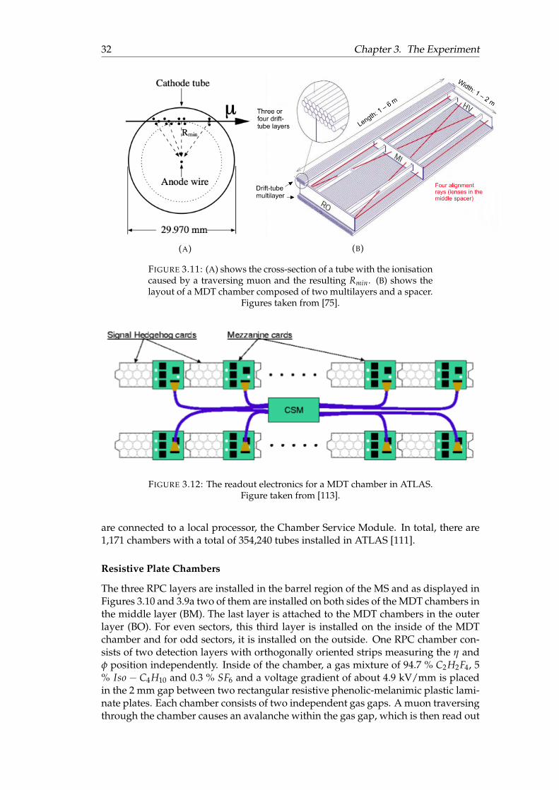
32 Chapter 3. The Experiment
(A) (B)
FIGURE 3.11: (A) shows the cross-section of a tube with the ionisationcaused by a traversing muon and the resulting Rmin. (B) shows thelayout of a MDT chamber composed of two multilayers and a spacer.
Figures taken from [75].
FIGURE 3.12: The readout electronics for a MDT chamber in ATLAS.Figure taken from [113].
are connected to a local processor, the Chamber Service Module. In total, there are1,171 chambers with a total of 354,240 tubes installed in ATLAS [111].
Resistive Plate Chambers
The three RPC layers are installed in the barrel region of the MS and as displayed inFigures 3.10 and 3.9a two of them are installed on both sides of the MDT chambers inthe middle layer (BM). The last layer is attached to the MDT chambers in the outerlayer (BO). For even sectors, this third layer is installed on the inside of the MDTchamber and for odd sectors, it is installed on the outside. One RPC chamber con-sists of two detection layers with orthogonally oriented strips measuring the η andφ position independently. Inside of the chamber, a gas mixture of 94.7 % C2H2F4, 5% Iso − C4H10 and 0.3 % SF6 and a voltage gradient of about 4.9 kV/mm is placedin the 2 mm gap between two rectangular resistive phenolic-melanimic plastic lami-nate plates. Each chamber consists of two independent gas gaps. A muon traversingthrough the chamber causes an avalanche within the gas gap, which is then read out
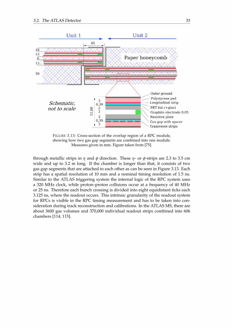
3.2. The ATLAS Detector 33
FIGURE 3.13: Cross-section of the overlap region of a RPC module,showing how two gas gap segments are combined into one module.
Measures given in mm. Figure taken from [75].
through metallic strips in η and φ direction. These η- or φ-strips are 2.3 to 3.5 cmwide and up to 3.2 m long. If the chamber is longer than that, it consists of twogas gap segments that are attached to each other as can be seen in Figure 3.13. Eachstrip has a spatial resolution of 10 mm and a nominal timing resolution of 1.5 ns.Similar to the ATLAS triggering system the internal logic of the RPC system usesa 320 MHz clock, while proton–proton collisions occur at a frequency of 40 MHzor 25 ns. Therefore each bunch crossing is divided into eight equidistant ticks each3.125 ns, where the readout occurs. This intrinsic granularity of the readout systemfor RPCs is visible in the RPC timing measurement and has to be taken into con-sideration during track reconstruction and calibrations. In the ATLAS MS, there areabout 3600 gas volumes and 370,000 individual readout strips combined into 606chambers [114, 115].

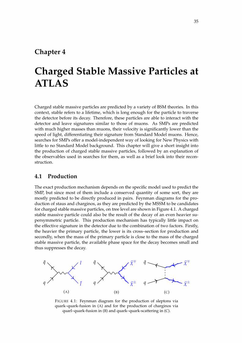
35
Chapter 4
Charged Stable Massive Particles atATLAS
Charged stable massive particles are predicted by a variety of BSM theories. In thiscontext, stable refers to a lifetime, which is long enough for the particle to traversethe detector before its decay. Therefore, these particles are able to interact with thedetector and leave signatures similar to those of muons. As SMPs are predictedwith much higher masses than muons, their velocity is significantly lower than thespeed of light, differentiating their signature from Standard Model muons. Hence,searches for SMPs offer a model-independent way of looking for New Physics withlittle to no Standard Model background. This chapter will give a short insight intothe production of charged stable massive particles, followed by an explanation ofthe observables used in searches for them, as well as a brief look into their recon-struction.
4.1 Production
The exact production mechanism depends on the specific model used to predict theSMP, but since most of them include a conserved quantity of some sort, they aremostly predicted to be directly produced in pairs. Feynman diagrams for the pro-duction of staus and charginos, as they are predicted by the MSSM to be candidatesfor charged stable massive particles, on tree level are shown in Figure 4.1. A chargedstable massive particle could also be the result of the decay of an even heavier su-persymmetric particle. This production mechanism has typically little impact onthe effective signature in the detector due to the combination of two factors. Firstly,the heavier the primary particle, the lower is its cross–section for production andsecondly, when the mass of the primary particle is close to the mass of the chargedstable massive particle, the available phase space for the decay becomes small andthus suppresses the decay.
q
q
l
l
(A)
q
q
χ±
χ∓
(B)
q χ±
q χ∓
(C)
FIGURE 4.1: Feynman diagram for the production of sleptons viaquark–quark-fusion in (A) and for the production of charginos via
quarl–quark-fusion in (B) and quark–quark-scattering in (C).
36 Chapter 4. Charged Stable Massive Particles at ATLAS
While a single production channel for SMPs is theoretically possible, the productioncross–section is proportional to the decay width in this case and therefore propor-tional to the inverse of the lifetime. In order to achieve lifetimes long enough tobe considered stable, the cross–section becomes negligible. Furthermore, it is pos-sible for a charged stable massive particle to be produced in combination with anuncharged stable massive particle. This may occur when they have almost the samemass and the neutral particle is the lightest particle with a new conserved quantumnumber. In the MSSM, this could be the case for the combination of the lightestneutralino and chargino. As a result, the neutral particle would most likely not bedetectable, leaving only a missing transverse energy E miss
T as its signature [67].
4.2 Observables
Charged stable massive particles offer an appealing approach for a search for BSMtheories. As they are electrically charged, they interact with the detector materialand therefore leave a signal that can be measured. The high predicted mass leads tothe expectation of large ionisation energy losses in the ID and a velocity significantlylower than the speed of light (βγ ≤ 0.9 [116]) that can be used for identification.Thus, the difference between the expected time of arrival1 and the timing informa-tion of the interaction with the detector can be a useful measure. Since no StandardModel process leads to similar signatures, the background for an analysis lookingfor charged stable massive particles is dominated by detector mismeasurements.
4.2.1 Ionisation Energy Loss
A charged particle traversing the detector interacts with the electrons of the detectormaterial and by exciting or ionising them, the traversing particle deposits some of itsenergy in the detector material. This energy loss is referred to as ionisation energyloss or 〈 dE
dx 〉. The ID deployed in ATLAS is capable of measuring 〈 dEdx 〉 with its pixel
detector and TRT, while the SCT does not provide a 〈 dEdx 〉 measurement. The mean
of the energy loss per travelled distance of a particle with energy E, charge z andvelocity v can be calculated using the Bethe–Bloch–formula shown in Equation 4.1[117, 118]. ⟨
dEdx
⟩=
4πe4z2nmec2β2
(12
ln(
2mec2β2γ2Tmax
Ie
)− β2 − δ
2
)(4.1)
The electron density of the material is denoted with n, while me and e symbolise therest-mass and the charge of electrons, respectively. The mean ionisation potentialis described by Ie and δ is a material constant accounting for density effects. Thespeed of light is denoted with c. As can be seen in Equation 4.2a, β results from theratio of the velocity v and the speed of light, while the Lorentz factor γ is definedin Equation 4.2b. Tmax denotes the maximum energy transfer a single electron canreceive. If the traversing particle is much heavier than the electron, Tmax is given byEquation 4.2c.
1Particles traversing ATLAS are expected to travel at the speed of light.
4.2. Observables 37
β :=vc
γ :=1√
1− β2Tmax = 2mec2β2γ2 (4.2a-c)
Since Equation 4.1 is only dependent on variables specific to the material and thevelocity of the traversing particle, the 〈 dE
dx 〉measurement serves as a way to calculatethe velocity of the traversing particle. The pixel detector gives one 〈 dE
dx 〉 measure-ment per layer and thus four individual measurements of the ionisation energy. Byaveraging them, one can get the Most Probable Value (MPV). Since it is known that〈 dE
dx 〉 is Landau distributed, the MPV differs from the mean of Equation 4.1. There-fore, an empiric Bethe–Bloch–formula is used to get a relation between the MPV of〈 dE
dx 〉 and the velocity. This empiric formula can be seen in Equation 4.3.
MPV dEdx
=A
(βγ)C + B (4.3)
A, B and C are calibration constants determined by low-momentum pions, kaonsand protons reconstructed by ATLAS in low-luminosity runs [116] and as shown inEquations 4.2a and 4.2b, βγ is only dependent on the velocity of the traversing par-ticle and therefore serves as a measure for it. In order the reduce the impact of thetales of the Landau distribution and to ensure that the mean of the 〈 dE
dx 〉 measure-ments gives a good estimate for the MPV dE
dx, it is calculated disregarding the highest
〈 dEdx 〉measurement. In combination with the measured momentum, p, the ID is even
able to perform a calculation of the rest-mass m0 of the traversing particle by usingEquation 4.4 [119].
m0 =p
βγ(4.4)
4.2.2 Time-of-Flight Measurement
Another independent approach to measure the velocity, or β, is to evaluate the timeit took for the particle to travel from the interaction point to a detector element at dis-tance d. This approach is referred to as Time-of-Flight (ToF) measurement. Particleswith the same energy but different masses also differ in their β, which means thatheavier particles have a smaller β and therefore need more time to reach a specificelement of the detector. Thus, a variable t0 is introduced, given in Equation 4.5a,which measures the difference between the actual time of flight ToFa and the time offlight of a particle traversing the detector at the speed of light (β = 1) ToFc. As canbe seen in Equation 4.5b, the t0 value can be used to calculate β. By using additionalinformation about the momentum p of the traversing particle, its rest-mass m0 canthen be calculated according to Equation 4.4.
t0 = ToFa − ToFc = ToFa −dc
β =d
ToFa· 1
c=
dd + t0 · c
(4.5a-b)
Due to their large distance from the interaction point and the available timing infor-mation, the tile calorimeter as well as the MDT tubes and RPC strips of the MS aresuitable detector elements to perform a ToF, and thereby a measurement of β.
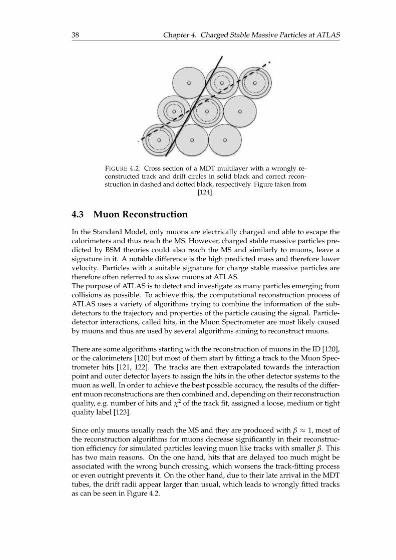
38 Chapter 4. Charged Stable Massive Particles at ATLAS
FIGURE 4.2: Cross section of a MDT multilayer with a wrongly re-constructed track and drift circles in solid black and correct recon-struction in dashed and dotted black, respectively. Figure taken from
[124].
4.3 Muon Reconstruction
In the Standard Model, only muons are electrically charged and able to escape thecalorimeters and thus reach the MS. However, charged stable massive particles pre-dicted by BSM theories could also reach the MS and similarly to muons, leave asignature in it. A notable difference is the high predicted mass and therefore lowervelocity. Particles with a suitable signature for charge stable massive particles aretherefore often referred to as slow muons at ATLAS.The purpose of ATLAS is to detect and investigate as many particles emerging fromcollisions as possible. To achieve this, the computational reconstruction process ofATLAS uses a variety of algorithms trying to combine the information of the sub-detectors to the trajectory and properties of the particle causing the signal. Particle-detector interactions, called hits, in the Muon Spectrometer are most likely causedby muons and thus are used by several algorithms aiming to reconstruct muons.
There are some algorithms starting with the reconstruction of muons in the ID [120],or the calorimeters [120] but most of them start by fitting a track to the Muon Spec-trometer hits [121, 122]. The tracks are then extrapolated towards the interactionpoint and outer detector layers to assign the hits in the other detector systems to themuon as well. In order to achieve the best possible accuracy, the results of the differ-ent muon reconstructions are then combined and, depending on their reconstructionquality, e.g. number of hits and χ2 of the track fit, assigned a loose, medium or tightquality label [123].
Since only muons usually reach the MS and they are produced with β ≈ 1, most ofthe reconstruction algorithms for muons decrease significantly in their reconstruc-tion efficiency for simulated particles leaving muon like tracks with smaller β. Thishas two main reasons. On the one hand, hits that are delayed too much might beassociated with the wrong bunch crossing, which worsens the track-fitting processor even outright prevents it. On the other hand, due to their late arrival in the MDTtubes, the drift radii appear larger than usual, which leads to wrongly fitted tracksas can be seen in Figure 4.2.
4.3. Muon Reconstruction 39
This creates the problem that charged stable massive particles with a high-enoughmass would simply not be reconstructed in ATLAS with decent efficiency and couldtherefore not be analysed. To resolve this issue, a new reconstruction algorithmcalled MUGIRLLOWBETA [125, 126] was introduced, applying a number of differenttechniques in contrast to the other muon reconstruction algorithms:
• By additionally considering the next bunch crossing, hits and especially triggerhits are recovered and used for reconstruction.
• Due to its close proximity to the interaction point, the ToF measured in the IDdoes not differ much for particles with a small β and particles propagating withat speed of light. Thus, measurements in the ID are less likely to be assignedto the wrong bunch crossing. Consequently, the reconstruction starts in theID and extrapolates to the outer detector layers, where additional hits can beassigned with high efficiency.
• Instead of assuming β ≈ 1, MUGIRLLOWBETA estimates β from the hit timingin the RPC strips and thus prevents the misidentification of the slow particleas a muon.
• β is treated as a free parameter when the MDT hits are fitted with a track,which allows for variable drift radii. The track with the best fitting result isthen chosen.
As can be seen in Figure 4.3, MUGIRLLOWBETA is able to extend the range inwhich slow muons can be reconstructed with high efficiency greatly into areas withsmaller β.
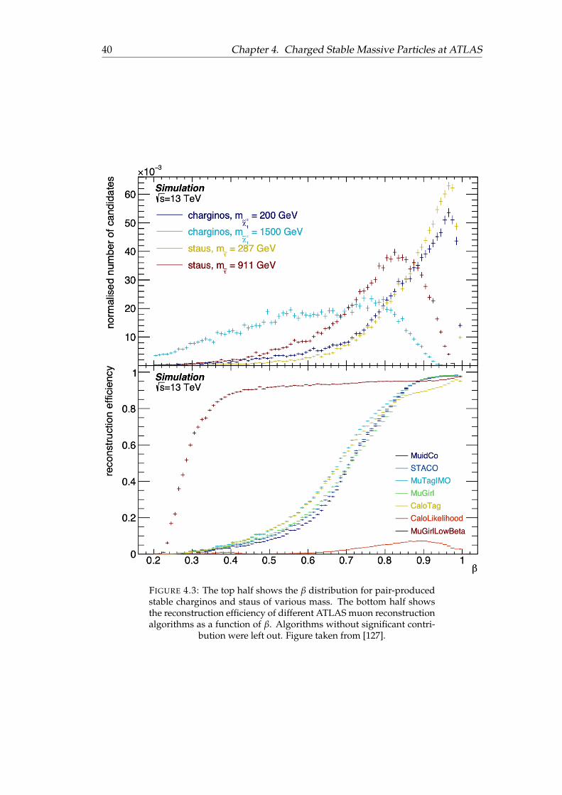
40 Chapter 4. Charged Stable Massive Particles at ATLAS
FIGURE 4.3: The top half shows the β distribution for pair-producedstable charginos and staus of various mass. The bottom half showsthe reconstruction efficiency of different ATLAS muon reconstructionalgorithms as a function of β. Algorithms without significant contri-
bution were left out. Figure taken from [127].
41
Chapter 5
Calibration of the TimingMeasurement of the ATLAS MuonSpectrometer
As already stated in the previous chapters, searches for charged stable massive par-ticles offer a model-independent approach to a search for BSM physics with little tono Standard Model background. Thus, detector mismeasurements are the leadingbackground for such analyses. A good understanding of the detector systems andtheir β resolution is therefore very important and by improving this β resolution,the chance detecting a charged stable massive particle can be increased or strongerexclusion limits can be obtained. The calibration of the 〈 dE
dx 〉 measurement can beadopted from [116], but no other search in ATLAS relies on a β measurement via aToF measurement in the tile calorimeter or Muon Spectrometer and thus a calibra-tion strategy for the ToF measurement has to be developed. A timing calibration ofthe ToF and according β measurement of the tile calorimeter can be found in Refer-ence [128]. The work at hand focusses on the timing calibration of the measurementin the ATLAS Muon Spectrometer, which shall be described in this chapter.
The timing information of a hit in a single element of the Muon Spectrometer isswayed by several influences, which is the reason why different calibration steps areneeded. Each calibration step tries to get rid of an effect distorting the timing mea-surement. Since muons are charged and reach the MS, they can be detected by it andused as a probe for such biases in the timing measurement. Due to their low mass,muons above a certain energy threshold traverse the detector with almost the speedof light and thus have β = 1. Therefore, they should be measured with t0 = 0 ns.Due to the fact that a detector performs measurements with an uncertainty: insteadof t0 = 0 ns for each muon, a Gaussian distribution with its mean at t0 = 0 ns isexpected as the result of the ToF measurement of several muons.
The general calibration strategy is therefore to analyse t0 distributions for differentdependencies and then apply a Gaussian fit to them. The mean of the fit can thenbe used as a correction constant for the specific dependency and the t0 value of eachhit can be calibrated step by step according to Equation 5.1. Hereby, tin
0 is the uncal-ibrated t0 value of the hit, tcorr
0 is the correction constant of a specific calibration stepand tout
0 is the calibrated t0 of the specific hit.
tout0 = tin
0 − ∑calibrations
tcorr0 (5.1)
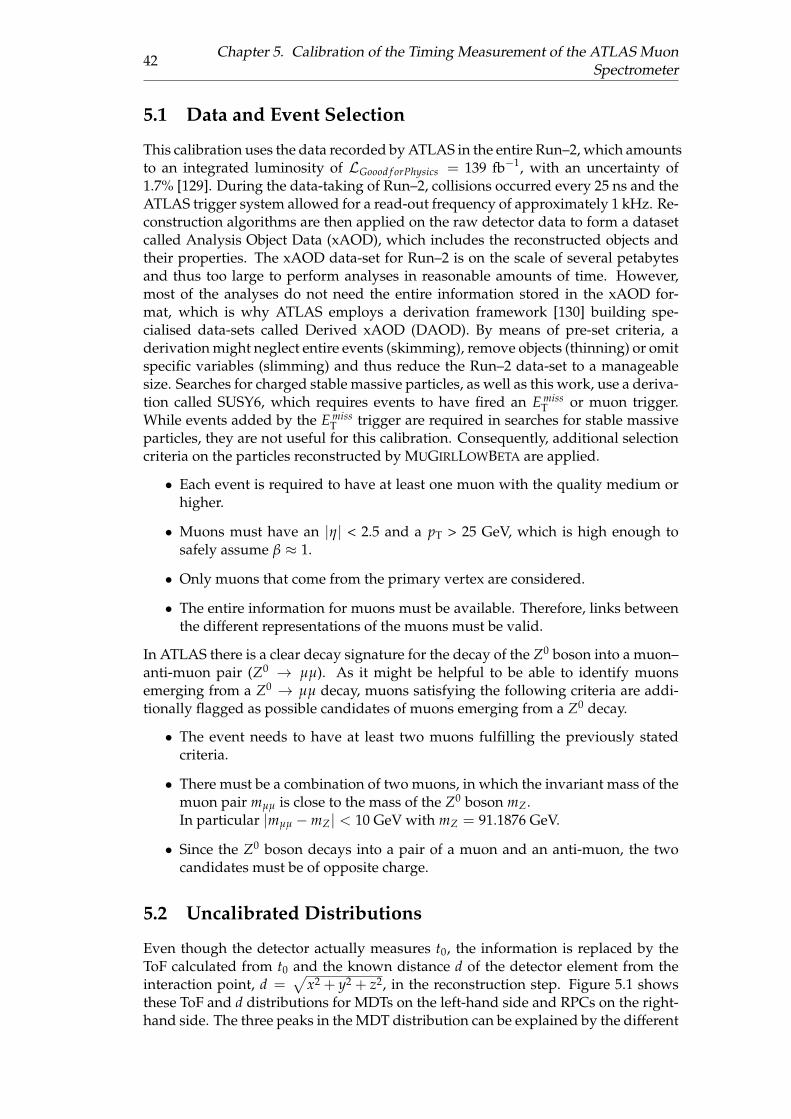
42Chapter 5. Calibration of the Timing Measurement of the ATLAS Muon
Spectrometer
5.1 Data and Event Selection
This calibration uses the data recorded by ATLAS in the entire Run–2, which amountsto an integrated luminosity of LGoood f orPhysics = 139 fb−1, with an uncertainty of1.7% [129]. During the data-taking of Run–2, collisions occurred every 25 ns and theATLAS trigger system allowed for a read-out frequency of approximately 1 kHz. Re-construction algorithms are then applied on the raw detector data to form a datasetcalled Analysis Object Data (xAOD), which includes the reconstructed objects andtheir properties. The xAOD data-set for Run–2 is on the scale of several petabytesand thus too large to perform analyses in reasonable amounts of time. However,most of the analyses do not need the entire information stored in the xAOD for-mat, which is why ATLAS employs a derivation framework [130] building spe-cialised data-sets called Derived xAOD (DAOD). By means of pre-set criteria, aderivation might neglect entire events (skimming), remove objects (thinning) or omitspecific variables (slimming) and thus reduce the Run–2 data-set to a manageablesize. Searches for charged stable massive particles, as well as this work, use a deriva-tion called SUSY6, which requires events to have fired an E miss
T or muon trigger.While events added by the E miss
T trigger are required in searches for stable massiveparticles, they are not useful for this calibration. Consequently, additional selectioncriteria on the particles reconstructed by MUGIRLLOWBETA are applied.
• Each event is required to have at least one muon with the quality medium orhigher.
• Muons must have an |η| < 2.5 and a pT > 25 GeV, which is high enough tosafely assume β ≈ 1.
• Only muons that come from the primary vertex are considered.
• The entire information for muons must be available. Therefore, links betweenthe different representations of the muons must be valid.
In ATLAS there is a clear decay signature for the decay of the Z0 boson into a muon–anti-muon pair (Z0 → µµ). As it might be helpful to be able to identify muonsemerging from a Z0 → µµ decay, muons satisfying the following criteria are addi-tionally flagged as possible candidates of muons emerging from a Z0 decay.
• The event needs to have at least two muons fulfilling the previously statedcriteria.
• There must be a combination of two muons, in which the invariant mass of themuon pair mµµ is close to the mass of the Z0 boson mZ.In particular |mµµ −mZ| < 10 GeV with mZ = 91.1876 GeV.
• Since the Z0 boson decays into a pair of a muon and an anti-muon, the twocandidates must be of opposite charge.
5.2 Uncalibrated Distributions
Even though the detector actually measures t0, the information is replaced by theToF calculated from t0 and the known distance d of the detector element from theinteraction point, d =
√x2 + y2 + z2, in the reconstruction step. Figure 5.1 shows
these ToF and d distributions for MDTs on the left-hand side and RPCs on the right-hand side. The three peaks in the MDT distribution can be explained by the different
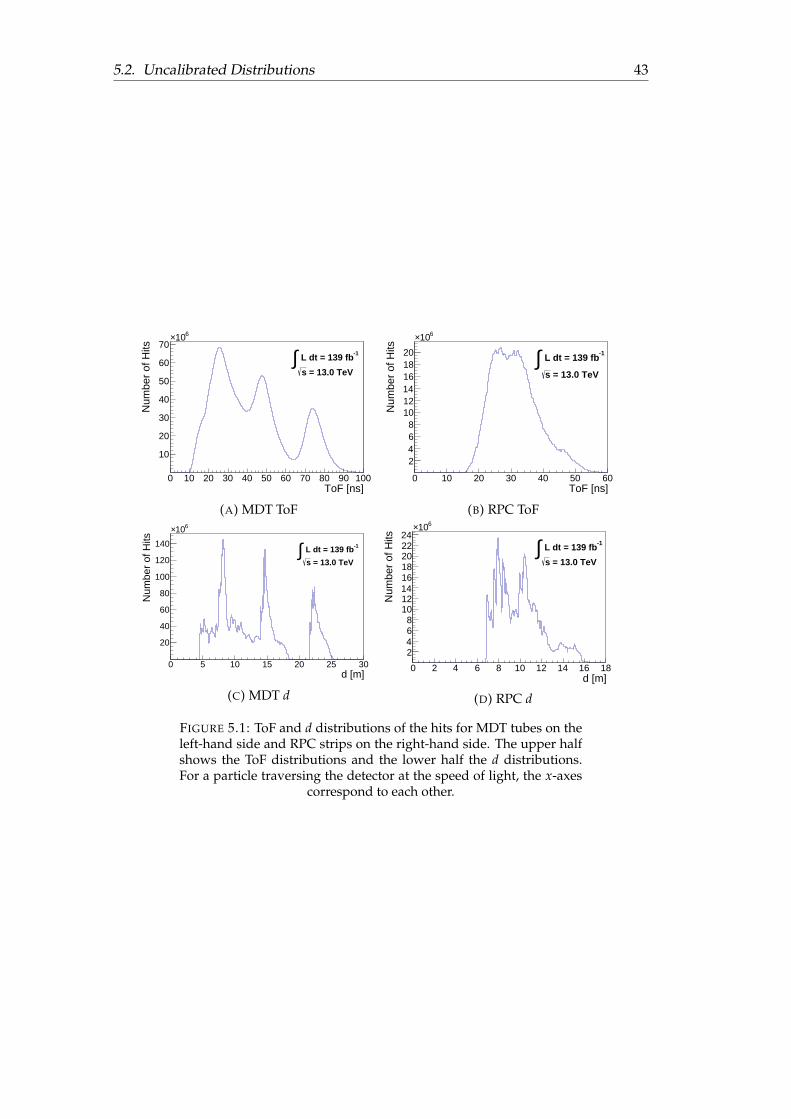
5.2. Uncalibrated Distributions 43
0 10 20 30 40 50 60 70 80 90 100ToF [ns]
10
20
30
40
50
60
70610×
Num
ber
of H
its -1 L dt = 139 fb∫ = 13.0 TeVs
(A) MDT ToF
0 10 20 30 40 50 60ToF [ns]
2468
101214161820
610×
Num
ber
of H
its -1 L dt = 139 fb∫ = 13.0 TeVs
(B) RPC ToF
0 5 10 15 20 25 30d [m]
20
40
60
80
100
120
140
610×
Num
ber
of H
its
-1 L dt = 139 fb∫ = 13.0 TeVs
(C) MDT d
0 2 4 6 8 10 12 14 16 18d [m]
2468
1012141618202224
610×
Num
ber
of H
its -1 L dt = 139 fb∫ = 13.0 TeVs
(D) RPC d
FIGURE 5.1: ToF and d distributions of the hits for MDT tubes on theleft-hand side and RPC strips on the right-hand side. The upper halfshows the ToF distributions and the lower half the d distributions.For a particle traversing the detector at the speed of light, the x-axes
correspond to each other.
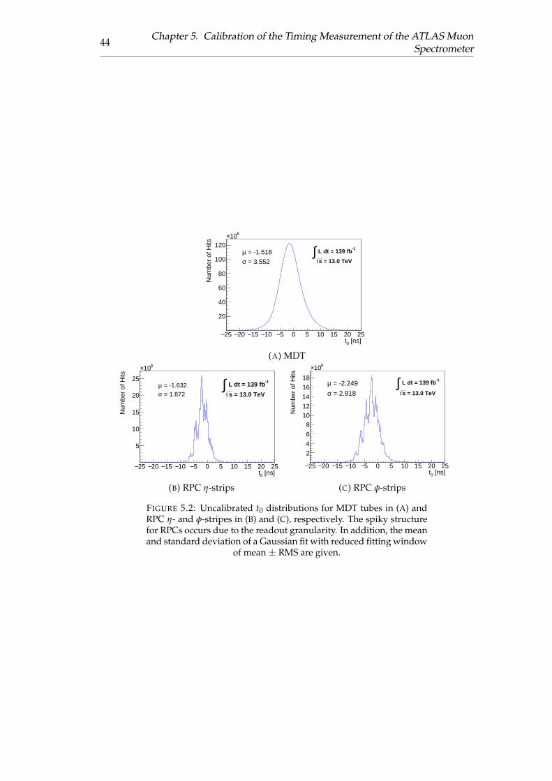
44Chapter 5. Calibration of the Timing Measurement of the ATLAS Muon
Spectrometer
25− 20− 15− 10− 5− 0 5 10 15 20 25 [ns]0t
20
40
60
80
100
120
610×
Num
ber
of H
its
= -1.518µ = 3.552σ
-1 L dt = 139 fb∫ = 13.0 TeVs
(A) MDT
25− 20− 15− 10− 5− 0 5 10 15 20 25 [ns]0t
5
10
15
20
25
610×
Num
ber
of H
its
= -1.632µ = 1.872σ
-1 L dt = 139 fb∫ = 13.0 TeVs
(B) RPC η-strips
25− 20− 15− 10− 5− 0 5 10 15 20 25 [ns]0t
24
68
101214
1618
610×
Num
ber
of H
its
= -2.249µ = 2.918σ
-1 L dt = 139 fb∫ = 13.0 TeVs
(C) RPC φ-strips
FIGURE 5.2: Uncalibrated t0 distributions for MDT tubes in (A) andRPC η- and φ-stripes in (B) and (C), respectively. The spiky structurefor RPCs occurs due to the readout granularity. In addition, the meanand standard deviation of a Gaussian fit with reduced fitting window
of mean ± RMS are given.
5.2. Uncalibrated Distributions 45
detector layers. The first peak includes the layers of the barrel region and the EI ofthe end-cap system. The second peak results from the EM and the third from theEO. Since there are no RPCs in the end-caps, the distance from the interaction pointto the detector element, and accordingly the ToF, has a lower upper bound and thepeak structure of the MDT distribution can not be observed. The readout granular-ity mentioned in Section 3.2.3 leads to the less smooth nature of the ToF distributionfor the RPCs.
The t0 values can be calculated by reverse engineering the ToF calculation follow-ing Equation 4.5a, which leads to the uncalibrated t0 distributions for MDT tubesand RPCs, divided into η- and φ-strips, depicted in Figure 5.2. The effect of the read-out granularity with 3.125 ns can be seen very clearly in Figures 5.2b and 5.2c. Toaccount for the position of the hit within the strip, a calculated propagation time issubtracted, which leads to distributions of the t0 values around peaks determined bythe readout granularity. RPC η- and φ-strips possess individual readout electronicsand thus their t0 distributions may differ. This difference can easily be seen by com-paring Figure 5.2b and Figure 5.2c. Regarding the RPC φ-strips, the mean is furthershifted from t0 = 0 ns and the width is significantly bigger than for RPC η-strips. Itis therefore useful to treat RPC η- and φ-strips as separate detector systems for thecalibration steps in this chapter. Even with this spiky nature, the general shape ofthe t0 distributions resembles the expected Gaussian shape. The distributions canthus be fitted with a Gaussian defined in Equation 5.2.
f (x) = A · e(x−µ)2
2σ2 (5.2)
A resembles the height of the function’s peak and can mostly be ignored in this work,µ gives the position of the peak on the x-axis and also indicates the mean of the func-tion. The standard deviation σ controls the width of the function and is therefore animportant measure of the resolution of the fitted distribution. The mean t0 and theresolution σ quoted in Figure 5.2, and similar figures in this chapter, correspond toµ and σ of Equation 5.2, respectively.
While the shapes of the distributions depicted in Figure 5.2 comply with the ex-pected Gaussian shape in general, their centre is clearly not at t0 = 0 ns. The aimof this calibration is to correctly centre the t0 distribution for each detector systemat t0 = 0 ns and to make them as narrow as possible. To achieve this, the follow-ing sections will look at different dependencies of the t0 measurement and introducecalibration steps to account for them. Since the calibrations are considered to be in-dependent of each other, the final calibrated t0 value for every hit can be calculatedas introduced in Equation 5.1.
As the ToF measurement aims at identifying traversing charged stable massive par-ticles by their smaller β, it is useful to take a look at how β can be calculated fromthe t0 measurement. Firstly, a traversing particle interacts with several detector ele-ments and thus leads to several individual t0 measurements. Since different detec-tor elements might differ in their accuracy, it is beneficial to determine the β of thetraversing particle as a weighted average of those measurements. Additionally, asstated in Equation 4.5b: βi ∝ t−1
0,i and thus it is easier to take the uncertainty σt0,iof the individual timing information t0,i into account when calculating a weighted
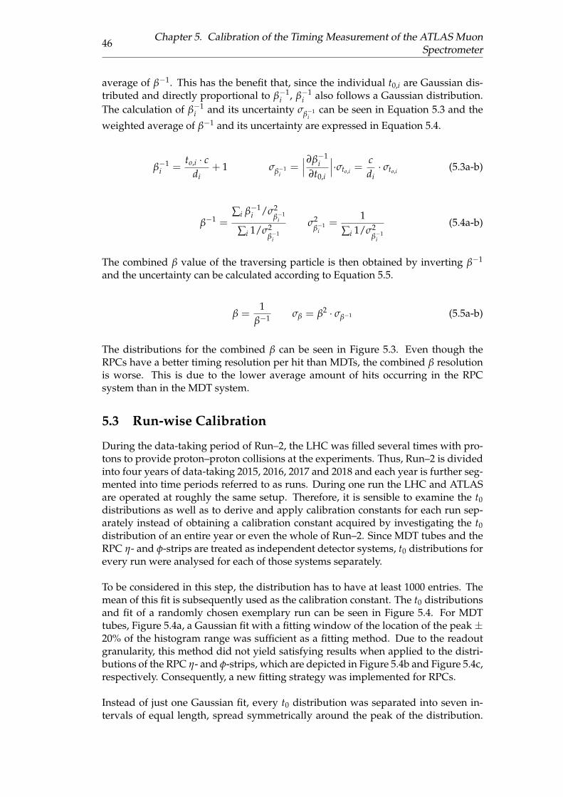
46Chapter 5. Calibration of the Timing Measurement of the ATLAS Muon
Spectrometer
average of β−1. This has the benefit that, since the individual t0,i are Gaussian dis-tributed and directly proportional to β−1
i , β−1i also follows a Gaussian distribution.
The calculation of β−1i and its uncertainty σβ−1
ican be seen in Equation 5.3 and the
weighted average of β−1 and its uncertainty are expressed in Equation 5.4.
β−1i =
to,i · cdi
+ 1 σβ−1i
=∣∣∣∂β−1
i∂t0,i
∣∣∣·σto,i =cdi· σto,i (5.3a-b)
β−1 =∑i β−1
i /σ2β−1
i
∑i 1/σ2β−1
i
σ2β−1
i=
1∑i 1/σ2
β−1i
(5.4a-b)
The combined β value of the traversing particle is then obtained by inverting β−1
and the uncertainty can be calculated according to Equation 5.5.
β =1
β−1 σβ = β2 · σβ−1 (5.5a-b)
The distributions for the combined β can be seen in Figure 5.3. Even though theRPCs have a better timing resolution per hit than MDTs, the combined β resolutionis worse. This is due to the lower average amount of hits occurring in the RPCsystem than in the MDT system.
5.3 Run-wise Calibration
During the data-taking period of Run–2, the LHC was filled several times with pro-tons to provide proton–proton collisions at the experiments. Thus, Run–2 is dividedinto four years of data-taking 2015, 2016, 2017 and 2018 and each year is further seg-mented into time periods referred to as runs. During one run the LHC and ATLASare operated at roughly the same setup. Therefore, it is sensible to examine the t0distributions as well as to derive and apply calibration constants for each run sep-arately instead of obtaining a calibration constant acquired by investigating the t0distribution of an entire year or even the whole of Run–2. Since MDT tubes and theRPC η- and φ-strips are treated as independent detector systems, t0 distributions forevery run were analysed for each of those systems separately.
To be considered in this step, the distribution has to have at least 1000 entries. Themean of this fit is subsequently used as the calibration constant. The t0 distributionsand fit of a randomly chosen exemplary run can be seen in Figure 5.4. For MDTtubes, Figure 5.4a, a Gaussian fit with a fitting window of the location of the peak ±20% of the histogram range was sufficient as a fitting method. Due to the readoutgranularity, this method did not yield satisfying results when applied to the distri-butions of the RPC η- and φ-strips, which are depicted in Figure 5.4b and Figure 5.4c,respectively. Consequently, a new fitting strategy was implemented for RPCs.
Instead of just one Gaussian fit, every t0 distribution was separated into seven in-tervals of equal length, spread symmetrically around the peak of the distribution.
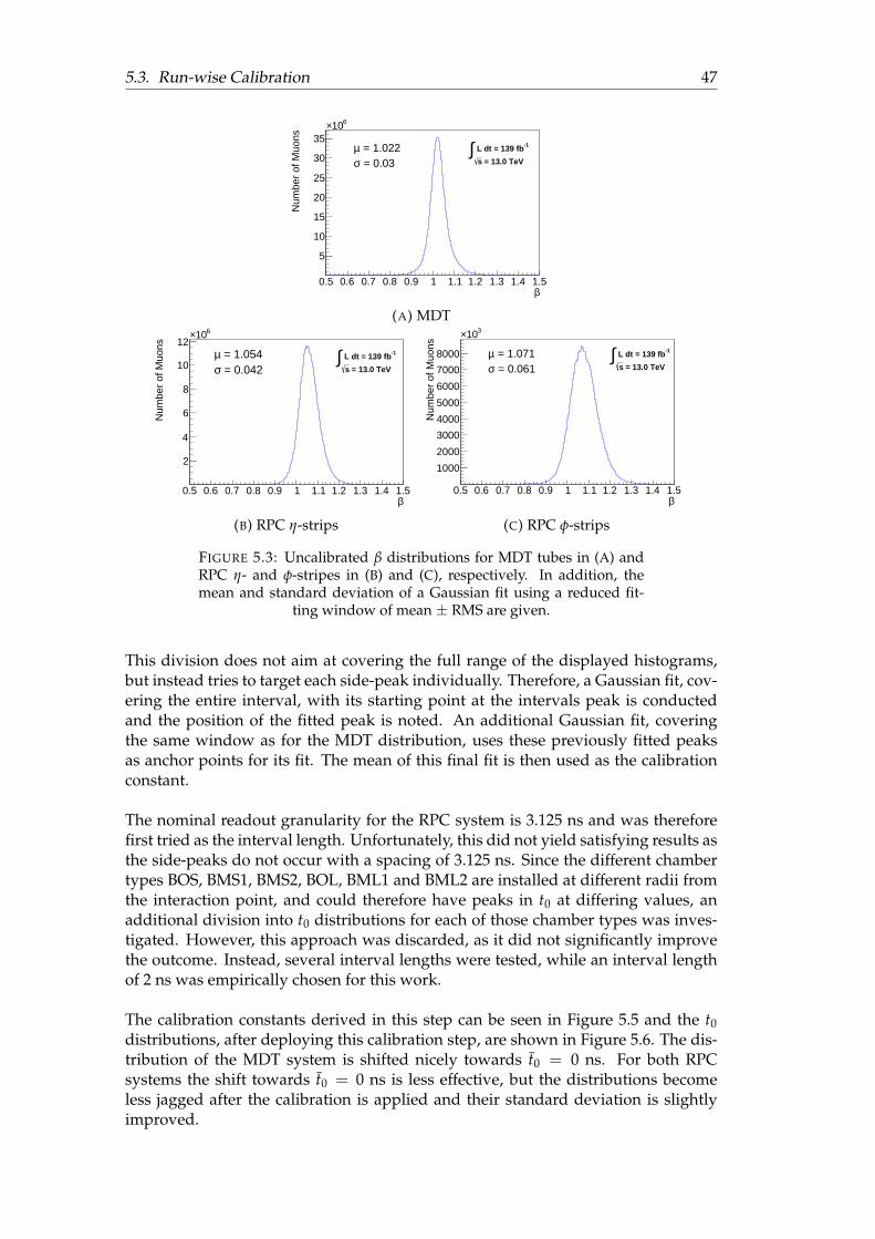
5.3. Run-wise Calibration 47
0.5 0.6 0.7 0.8 0.9 1 1.1 1.2 1.3 1.4 1.5β
5
10
15
20
25
30
35
610×
Num
ber
of M
uons
= 1.022µ = 0.03σ
-1 L dt = 139 fb∫ = 13.0 TeVs
(A) MDT
0.5 0.6 0.7 0.8 0.9 1 1.1 1.2 1.3 1.4 1.5β
2
4
6
8
10
12610×
Num
ber
of M
uons
= 1.054µ = 0.042σ
-1 L dt = 139 fb∫ = 13.0 TeVs
(B) RPC η-strips
0.5 0.6 0.7 0.8 0.9 1 1.1 1.2 1.3 1.4 1.5β
1000
2000
3000
4000
5000
6000
7000
8000
310×
Num
ber
of M
uons
= 1.071µ = 0.061σ
-1 L dt = 139 fb∫ = 13.0 TeVs
(C) RPC φ-strips
FIGURE 5.3: Uncalibrated β distributions for MDT tubes in (A) andRPC η- and φ-stripes in (B) and (C), respectively. In addition, themean and standard deviation of a Gaussian fit using a reduced fit-
ting window of mean ± RMS are given.
This division does not aim at covering the full range of the displayed histograms,but instead tries to target each side-peak individually. Therefore, a Gaussian fit, cov-ering the entire interval, with its starting point at the intervals peak is conductedand the position of the fitted peak is noted. An additional Gaussian fit, coveringthe same window as for the MDT distribution, uses these previously fitted peaksas anchor points for its fit. The mean of this final fit is then used as the calibrationconstant.
The nominal readout granularity for the RPC system is 3.125 ns and was thereforefirst tried as the interval length. Unfortunately, this did not yield satisfying results asthe side-peaks do not occur with a spacing of 3.125 ns. Since the different chambertypes BOS, BMS1, BMS2, BOL, BML1 and BML2 are installed at different radii fromthe interaction point, and could therefore have peaks in t0 at differing values, anadditional division into t0 distributions for each of those chamber types was inves-tigated. However, this approach was discarded, as it did not significantly improvethe outcome. Instead, several interval lengths were tested, while an interval lengthof 2 ns was empirically chosen for this work.
The calibration constants derived in this step can be seen in Figure 5.5 and the t0distributions, after deploying this calibration step, are shown in Figure 5.6. The dis-tribution of the MDT system is shifted nicely towards t0 = 0 ns. For both RPCsystems the shift towards t0 = 0 ns is less effective, but the distributions becomeless jagged after the calibration is applied and their standard deviation is slightlyimproved.
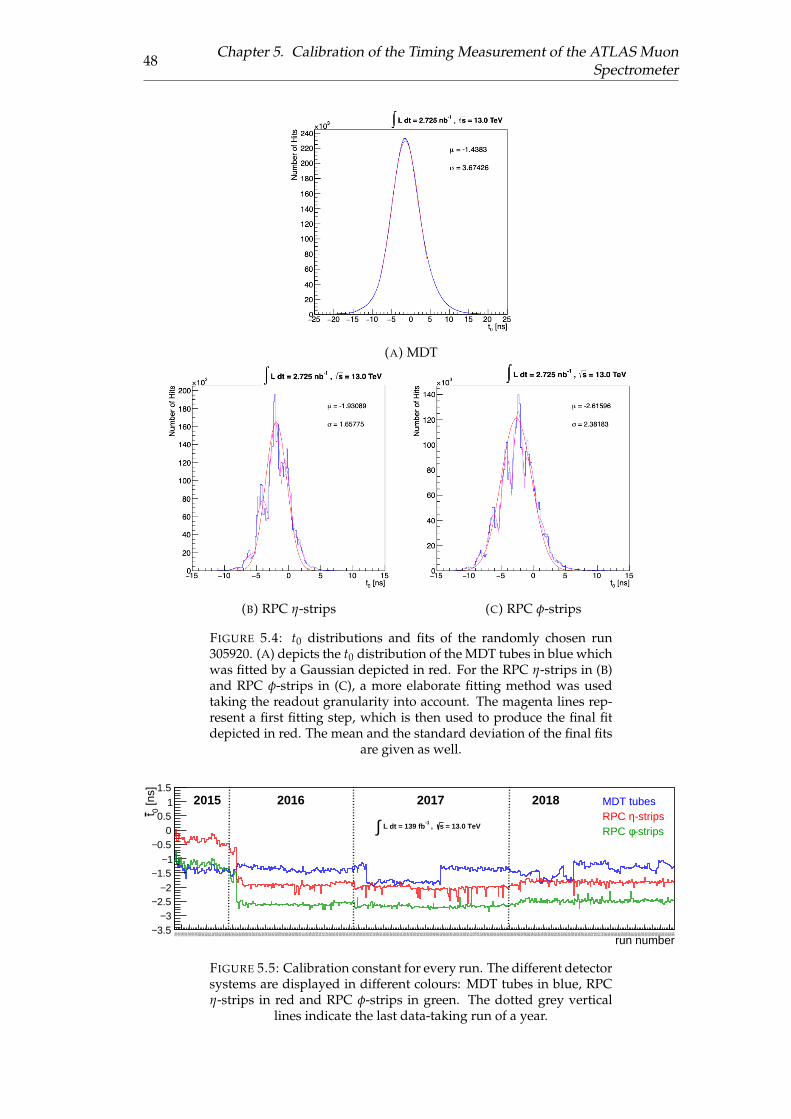
48Chapter 5. Calibration of the Timing Measurement of the ATLAS Muon
Spectrometer
(A) MDT
(B) RPC η-strips (C) RPC φ-strips
FIGURE 5.4: t0 distributions and fits of the randomly chosen run305920. (A) depicts the t0 distribution of the MDT tubes in blue whichwas fitted by a Gaussian depicted in red. For the RPC η-strips in (B)and RPC φ-strips in (C), a more elaborate fitting method was usedtaking the readout granularity into account. The magenta lines rep-resent a first fitting step, which is then used to produce the final fitdepicted in red. The mean and the standard deviation of the final fits
are given as well.
2762
6227
6329
2763
3627
6416
2765
1127
6689
2767
7827
6790
2769
5227
6954
2788
8027
8912
2789
6827
9169
2792
5927
9279
2792
8427
9345
2795
1527
9598
2796
8527
9764
2798
1327
9867
2799
2827
9932
2799
8428
0231
2802
7328
0319
2803
6828
0423
2804
6428
0500
2805
2028
0614
2806
7328
0753
2808
5328
0862
2809
5028
0977
2810
7028
1074
2810
7528
1317
2813
8528
1411
2826
2528
2631
2827
1228
2784
2829
9228
3074
2831
5528
3270
2834
2928
3608
2837
8028
4006
2841
5428
4213
2842
8528
4420
2844
2728
4484
2977
3029
8595
2986
0929
8633
2986
8729
8690
2987
7129
8773
2988
6229
8967
2990
5529
9144
2991
4729
9184
2992
4329
9584
3002
7930
0345
3004
1530
0418
3004
8730
0540
3005
7130
0600
3006
5530
0687
3007
8430
0800
3008
6330
0908
3019
1230
1915
3019
1830
1932
3019
7330
2053
3021
3730
2265
3022
6930
2300
3023
4730
2380
3023
9130
2393
3027
3730
2831
3028
7230
2919
3029
2530
2956
3030
0730
3079
3032
0130
3208
3032
6430
3266
3032
9130
3304
3033
3830
3421
3034
9930
3560
3036
3830
3832
3038
4630
3892
3039
4330
4006
3040
0830
4128
3041
7830
4198
3042
1130
4243
3043
0830
4337
3044
0930
4431
3044
9430
5380
3055
4330
5571
3056
1830
5671
3056
7430
5723
3057
2730
5735
3057
7730
5920
3062
6930
6278
3063
1030
6419
3064
4230
6448
3064
5130
7126
3071
9530
7259
3073
0630
7354
3073
5830
7394
3074
5430
7514
3075
3930
7569
3076
0130
7619
3076
5630
7710
3077
1630
7732
3078
6130
7935
3080
4730
8084
3093
7530
9390
3094
4030
9516
3096
4030
9674
3097
5931
0247
3102
4931
0341
3103
7031
0405
3104
6831
0473
3106
3431
0691
3107
3831
0809
3108
6331
0872
3109
6931
1071
3111
7031
1244
3112
8731
1321
3113
6531
1402
3114
7331
1481
3257
1332
5790
3264
4632
6468
3265
5132
6657
3266
9532
6834
3268
7032
6923
3269
4532
7057
3271
0332
7265
3273
4232
7490
3275
8232
7636
3276
6232
7745
3277
6132
7764
3278
6032
7862
3280
4232
8099
3282
2132
8263
3283
3332
8374
3283
9332
9716
3297
7832
9780
3298
2932
9835
3298
6932
9964
3300
2533
0074
3300
7933
0101
3301
6033
0166
3302
0333
0294
3304
7033
1033
3310
8233
1085
3311
2933
1215
3312
3933
1697
3317
1033
1742
3317
7233
1804
3318
2533
1860
3318
7533
1905
3319
5133
1975
3323
0333
2304
3327
2033
2896
3329
1533
2953
3329
5533
3181
3331
9233
3367
3333
8033
3426
3334
6933
3487
3335
1933
3650
3337
0733
3778
3338
2833
3853
3339
0433
3979
3339
9433
4264
3343
1733
4350
3343
8433
4413
3344
4333
4455
3344
8733
4564
3345
8033
4588
3346
3733
4678
3347
3733
4779
3348
4233
4849
3348
7833
4890
3349
0733
4960
3349
9333
5016
3350
2233
5056
3350
8233
5083
3351
3133
5170
3351
7733
5222
3352
8233
5290
3365
0633
6548
3365
6733
6630
3366
7833
6719
3367
8233
6832
3368
5233
6915
3369
2733
6944
3369
9833
7005
3370
5233
7107
3371
5633
7176
3372
1533
7263
3373
3533
7371
3374
0433
7451
3374
9133
7542
3376
6233
7705
3378
3333
8183
3382
2033
8259
3382
6333
8349
3383
7733
8480
3384
9833
8608
3386
7533
8712
3387
6733
8834
3388
4633
8897
3389
3333
8967
3389
8733
9037
3390
7033
9205
3393
4633
9387
3393
9633
9435
3395
0033
9535
3395
6233
9590
3397
5833
9849
3399
5734
0030
3400
7234
0368
3404
5334
8885
3488
9434
8895
3490
1134
9014
3490
3334
9051
3491
1134
9114
3491
6934
9268
3493
0934
9327
3493
3534
9451
3494
8134
9498
3495
2634
9533
3495
3434
9582
3495
9234
9637
3496
4634
9693
3498
4134
9842
3499
4434
9977
3500
1335
0067
3501
2135
0144
3501
6035
0184
3502
2035
0310
3503
6135
0440
3504
7935
0531
3506
8235
0749
3507
5135
0803
3508
4235
0848
3508
8035
0923
3510
6235
1160
3512
2335
1296
3513
2535
1359
3513
6435
1455
3515
5035
1628
3516
3635
1671
3516
9835
1832
3518
9435
1969
3520
5635
2107
3522
7435
2340
3523
9435
2436
3524
4835
2494
3525
1435
5261
3552
7335
5529
3555
4435
5563
3555
9935
5650
3556
5135
5754
3558
4835
5861
3558
7735
5995
3560
7735
6095
3561
2435
6177
3562
0535
6250
3562
5935
7193
3572
8335
7293
3573
5535
7409
3574
5135
7500
3575
3935
7620
3576
7935
7713
3577
5035
7772
3578
2135
7887
3579
6235
8031
3580
9635
8115
3581
7535
8215
3582
3335
8300
3583
2535
8333
3583
9535
8516
3585
4135
8577
3586
1535
8656
3589
8535
9010
3590
5835
9124
3591
7035
9171
3591
9135
9279
3592
8635
9310
3593
5535
9398
3594
4135
9472
3595
4135
9586
3595
9335
9623
3596
7735
9678
3597
1735
9735
3597
6635
9823
3598
7235
9918
3600
2636
0063
3601
2936
0161
3602
0936
0244
3602
9336
0309
3603
4836
0373
3604
0236
1738
3617
9536
1862
3622
0436
2297
3623
4536
2354
3623
8836
2445
3625
5236
2619
3626
6136
2776
3630
3336
3096
3631
2936
3198
3632
6236
3400
3636
6436
3710
3637
3836
3830
3639
1036
3947
3639
7936
4030
3640
7636
4098
3641
6036
4214
3642
92
run number3.5−
3−2.5−
2−1.5−
1−0.5−
00.5
11.5
[ns]
0t
MDT tubes-stripsηRPC -stripsφRPC
= 13.0 TeVs , -1
L dt = 139 fb∫
2015 2016 2017 2018
FIGURE 5.5: Calibration constant for every run. The different detectorsystems are displayed in different colours: MDT tubes in blue, RPCη-strips in red and RPC φ-strips in green. The dotted grey vertical
lines indicate the last data-taking run of a year.
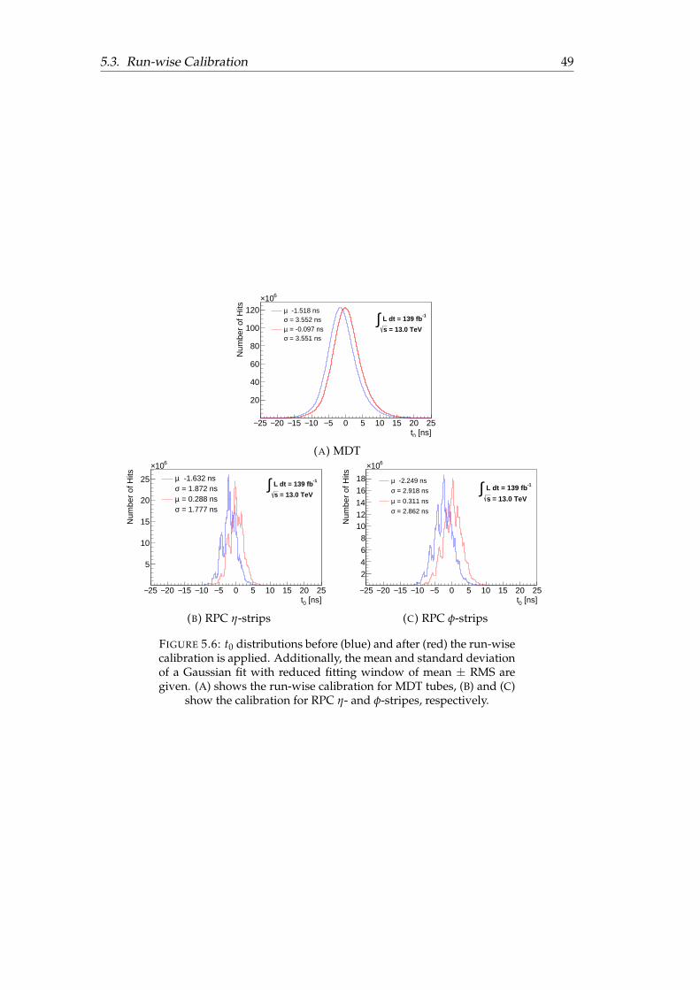
5.3. Run-wise Calibration 49
25− 20− 15− 10− 5− 0 5 10 15 20 25 [ns]0t
20
40
60
80
100
120
610×
Num
ber
of H
its -1.518 nsµ = 3.552 nsσ = -0.097 nsµ = 3.551 nsσ
-1 L dt = 139 fb∫ = 13.0 TeVs
(A) MDT
25− 20− 15− 10− 5− 0 5 10 15 20 25 [ns]0t
5
10
15
20
25
610×
Num
ber
of H
its -1.632 nsµ = 1.872 nsσ = 0.288 nsµ = 1.777 nsσ
-1 L dt = 139 fb∫ = 13.0 TeVs
(B) RPC η-strips
25− 20− 15− 10− 5− 0 5 10 15 20 25 [ns]0t
24
68
101214
1618
610×
Num
ber
of H
its
-2.249 nsµ = 2.918 nsσ = 0.311 nsµ = 2.862 nsσ
-1 L dt = 139 fb∫ = 13.0 TeVs
(C) RPC φ-strips
FIGURE 5.6: t0 distributions before (blue) and after (red) the run-wisecalibration is applied. Additionally, the mean and standard deviationof a Gaussian fit with reduced fitting window of mean ± RMS aregiven. (A) shows the run-wise calibration for MDT tubes, (B) and (C)
show the calibration for RPC η- and φ-stripes, respectively.
50Chapter 5. Calibration of the Timing Measurement of the ATLAS Muon
Spectrometer
5.4 Element-wise Calibration
The detector modules in the MS are composed of several individual elements. In thedata set used in the work at hand, muons satisfying the selection criteria interactedwith 354,347 separate MDT tubes and 371,616 different RPC stripes. Since addi-tional data about each element was necessary and only available for 354,292 MDTtubes and 371,333 RPC strips, only hits detected by those elements were consideredin this work.
As each element might differ in their t0 measurement, t0 distributions were imple-mented for each element separately and then fitted individually. Due to the largenumber of elements, the average number of entries per distribution is much smallerthan in the previous calibration step. On average, one MDT tube registered ap-proximately 69,000 hits and one RPC strip was hit on average nearly 10,000 times.Through this reduction in statistics, the distributions are not as smooth as in theprevious calibration step and thus harder to fit properly, as outliers hold a biggerinfluence on the fitting procedure and a too large amount of bins could affect the fitnegatively. To account for these problems, each t0 distribution was fitted nine timesand additional selection criteria were applied.
• As none of the used methods can be assumed to work reliably, elements withless than 40 registered hits where omitted in this step.
• RPC strips with an RMS greater than 10 ns show a peculiar t0 distribution andare thus ignored. No such cut was applied for MDTs.
• For the remaining elements, the t0 distribution was fitted nine times with thefollowing conditions:
– A Gaussian fit over the full range of [-25 ns, 25 ns].
– In order to lessen the effect of outliers, a Gaussian fit in a reduced fittingwindow of [-18 ns, 18 ns] is used, taking the time-spacing between twobunch crossings of 25 ns and some additional nanoseconds for the widthof the t0 distributions into account.
– To further lessen the impact of outliers, the fitting window of the Gaussianis reduced again to the location of the maximum ± the RMS provided bythe histogram.
– In order to account for elements with smaller statistics, the created his-togram is rebinned by adding neighbouring bins into one. Afterwards,the previous three steps are applied.
– A second rebinning, summing four neighbouring bins, is carried out andthe first three steps are applied.
• The fit with the smallest χ2 /ndof, with ndof being the number of degrees offreedom of the fit, is chosen as the best fit. When χ2 /ndof > 300 for the bestfit, none of the fits is considered a success.
• For the remaining elements the mean t0 and σt0 are stored and used as calibra-tion constants. When the element was not rejected but no fit was considered asuccess, the mean and RMS provided by the histogram are used as calibrationconstants.
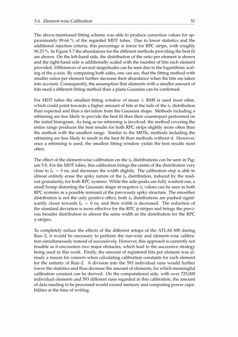
5.4. Element-wise Calibration 51
The above-mentioned fitting scheme was able to produce correction values for ap-proximately 99.64 % of the regarded MDT tubes. Due to lower statistics and theadditional rejection criteria, this percentage is lower for RPC strips, with roughly96.23 %. In Figure 5.7 the abundances for the different methods providing the best fitare shown. On the left-hand side, the distribution of the ratio per element is shownand the right-hand side is additionally scaled with the number of hits each elementprovided. Differences of several magnitudes can be seen due to the logarithmic scal-ing of the y-axis. By comparing both sides, one can see, that the fitting method withsmaller ratios per element further decrease their abundance when the hits are takeninto account. Consequently, the assumption that elements with a smaller amount ofhits need a different fitting method than a plane Gaussian can be confirmed.
For MDT tubes the smallest fitting window of mean ± RMS is used most often,which could point towards a higher amount of hits at the tails of the t0 distributionthan expected and thus a deviation from the Gaussian shape. Methods including arebinning are less likely to provide the best fit than their counterpart performed onthe initial histogram. As long as no rebinning is involved, the method covering theentire range produces the best results for both RPC strips slightly more often thanthe method with the smallest range. Similar to the MDTs, methods including therebinning are less likely to result in the best fit than methods without it. However,once a rebinning is used, the smallest fitting window yields the best results mostoften.
The effect of the element-wise calibration on the t0 distributions can be seen in Fig-ure 5.8. For the MDT tubes, this calibration brings the centre of the distribution veryclose to t0 = 0 ns, and decreases the width slightly. The calibration step is able toalmost entirely erase the spiky nature of the t0 distribution, induced by the read-out granularity, for both RPC systems. While the side-peaks are fully washed-out, asmall bump distorting the Gaussian shape at negative t0 values can be seen in bothRPC systems as a possible remnant of the previously spiky structure. The smootherdistribution is not the only positive effect, both t0 distributions are pushed signif-icantly closer towards t0 = 0 ns, and their width is decreased. The reduction ofthe standard deviation is more effective for the RPC φ-stripes and brings the previ-ous broader distribution to almost the same width as the distribution for the RPCη-stripes.
To completely reduce the effects of the different setups of the ATLAS MS duringRun–2, it would be necessary to perform the run-wise and element-wise calibra-tion simultaneously instead of successively. However, this approach is currently notfeasible as it encounters two major obstacles, which lead to the successive strategybeing used in this work. Firstly, the amount of registered hits per element was al-ready a reason for concern when calculating calibration constants for each elementfor the entirety of Run–2. A division into the 593 individual runs would furtherlower the statistics and thus decrease the amount of elements, for which meaningfulcalibration constant can be derived. On the computational side, with over 725,000individual elements and 593 different runs regarded in this calibration, the amountof data needing to be processed would exceed memory and computing power capa-bilities at the time of writing.
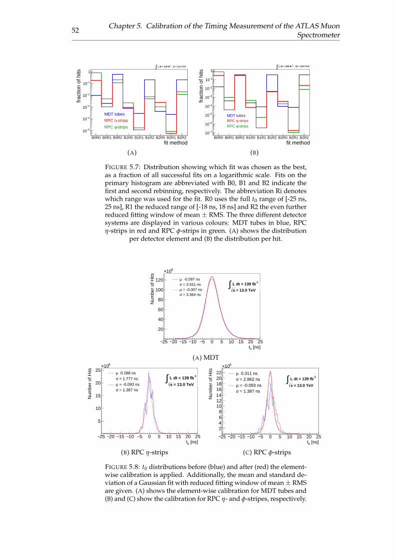
52Chapter 5. Calibration of the Timing Measurement of the ATLAS Muon
Spectrometer
B0R0 B0R1 B0R2 B1R0 B1R1 B1R2 B2R0 B2R1 B2R2
fit method
5−10
4−10
3−10
2−10
1−10
1
frac
tion
of h
its
MDT tubes
-stripsηRPC
-stripsφRPC
= 13.0 TeVs , -1 L dt = 139 fb∫
(A)
B0R0 B0R1 B0R2 B1R0 B1R1 B1R2 B2R0 B2R1 B2R2
fit method
7−10
6−10
5−10
4−10
3−10
2−10
1−10
1
frac
tion
of h
its
MDT tubes-stripsηRPC -stripsφRPC
= 13.0 TeVs , -1 L dt = 139 fb∫
(B)
FIGURE 5.7: Distribution showing which fit was chosen as the best,as a fraction of all successful fits on a logarithmic scale. Fits on theprimary histogram are abbreviated with B0, B1 and B2 indicate thefirst and second rebinning, respectively. The abbreviation Ri denoteswhich range was used for the fit. R0 uses the full t0 range of [-25 ns,25 ns], R1 the reduced range of [-18 ns, 18 ns] and R2 the even furtherreduced fitting window of mean ± RMS. The three different detectorsystems are displayed in various colours: MDT tubes in blue, RPCη-strips in red and RPC φ-strips in green. (A) shows the distribution
per detector element and (B) the distribution per hit.
25− 20− 15− 10− 5− 0 5 10 15 20 25 [ns]0t
20
40
60
80
100
120
610×
Num
ber
of H
its
-0.097 nsµ = 3.551 nsσ = -0.007 nsµ = 3.364 nsσ
-1 L dt = 139 fb∫ = 13.0 TeVs
(A) MDT
25− 20− 15− 10− 5− 0 5 10 15 20 25 [ns]0t
5
10
15
20
25610×
Num
ber
of H
its 0.288 nsµ = 1.777 nsσ = -0.093 nsµ = 1.387 nsσ
-1 L dt = 139 fb∫ = 13.0 TeVs
(B) RPC η-strips
25− 20− 15− 10− 5− 0 5 10 15 20 25 [ns]0t
2468
10121416182022
610×
Num
ber
of H
its 0.311 nsµ = 2.862 nsσ = -0.093 nsµ = 1.387 nsσ
-1 L dt = 139 fb∫
= 13.0 TeVs
(C) RPC φ-strips
FIGURE 5.8: t0 distributions before (blue) and after (red) the element-wise calibration is applied. Additionally, the mean and standard de-viation of a Gaussian fit with reduced fitting window of mean± RMSare given. (A) shows the element-wise calibration for MDT tubes and(B) and (C) show the calibration for RPC η- and φ-stripes, respectively.
5.5. Drift-time Calibration 53
5.5 Drift-time Calibration
A further dependency investigated is the correlation between the drift time tdrift ofcharges in the MDT tubes and the measured t0 value. The correlation between tdriftand t0 is shown in Figure 5.9a with the mean of a Gaussian fit performed for everytdrift-bin added in red.
Even though the nominal maximum for tdrift is 700 ns, recall Section 3.2.3, the figureclearly shows hits occurring with drift times exceeding this limitation. This is due tothe fact, that tdrift is actually not measured in the MDT but rather recalculated fromthe track fit during the reconstruction process. This calculation has some leniencywith regards to the physical barriers of tdrift, and thus hits measured with a verylarge t0 can be assigned a tdrift exceeding 700 ns. However, it is not sensible to as-sign a large tdrift value to a small t0 measurement. Instead, measurements of small t0values are assigned very low values of tdrift. This reconstruction process can explainthe decreasing mean of the Gaussian fit for low, and the rise in the mean for verylarge tdrift values. For drift times exceeding 765 ns, the Gaussian fit returns a meaneven exceeding the 10 ns range depicted in the figure. The mean has a clear upwardstrend with increasing tdrift on the left side of the figure and plateaus around 2 ns. Be-fore rising out of the range of the figure, it first dips towards negative t0 values. Asthe MDT tubes use a drift gas with a highly non-linear space-drift-time relation, thedecrease of the mean in the region 650 ns < tdrift < 725 ns can probably be attributedto an incorrect modelling of the drift gas during the reconstruction and the fact thattdrift is recalculated from the t0 measurement.
The calibration strategy is the same as in the previous steps. The mean of the Gaus-sian fit in each tdrift-bin is used as a correction constant for the t0 measurement of hitswithin the specific tdrift range. The results of an attempt to implement this strategycan be seen in Figure 5.9b. It is obvious, that this attempt did not yield the wantedresults. While the evolution of the mean with tdrift is less pronounced, which can beviewed as a success, the actual value of the mean differs largely from the expecta-tion of a flat line at t0 = 0 ns. The calibration seems to overcorrect and brings themean of the Gaussian fit for each tdrift-bin close to a line at t0 = −2 ns. The spreadof the mean at very high tdrift values can be explained by the t0 distribution of thatbin slowly reaching the limits of the produced histograms, which results in the fitstarting to yield unreliable results.
The effect of this calibration step on the t0 distribution of the MDT tubes can beseen in Figure 5.10. The overcorrection results in a shift of the mean of the distri-bution away from the targeted t0 = 0 ns. Due to the reduced tdrift dependency ofthe mean, the width of the distribution is decreased. As decreasing the width isone of the goals of this calibration and the general shift in t0 can be dealt with inthe following step, the calibration is still applied to the data. However, the cause ofthe overcorrection needs further investigation and the placement of this calibrationstep within the calibration order needs to be questioned since more calibration stepsfollowing this one would decrease the impact of the shift of t0.
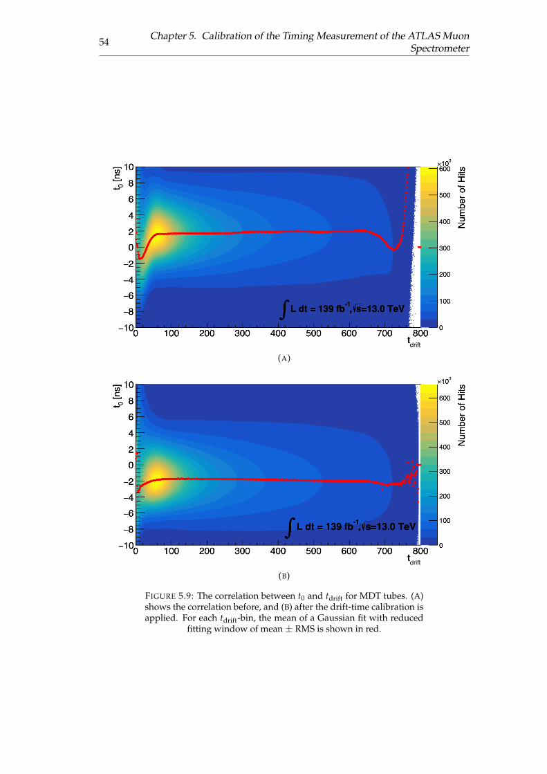
54Chapter 5. Calibration of the Timing Measurement of the ATLAS Muon
Spectrometer
(A)
(B)
FIGURE 5.9: The correlation between t0 and tdrift for MDT tubes. (A)shows the correlation before, and (B) after the drift-time calibration isapplied. For each tdrift-bin, the mean of a Gaussian fit with reduced
fitting window of mean ± RMS is shown in red.
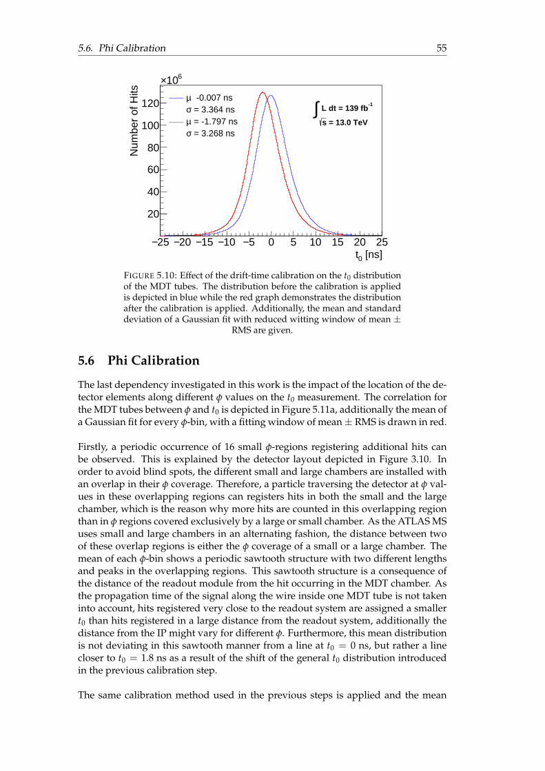
5.6. Phi Calibration 55
25− 20− 15− 10− 5− 0 5 10 15 20 25 [ns]0t
20
40
60
80
100
120
610×
Num
ber
of H
its -0.007 nsµ = 3.364 nsσ = -1.797 nsµ = 3.268 nsσ
-1 L dt = 139 fb∫
= 13.0 TeVs
FIGURE 5.10: Effect of the drift-time calibration on the t0 distributionof the MDT tubes. The distribution before the calibration is appliedis depicted in blue while the red graph demonstrates the distributionafter the calibration is applied. Additionally, the mean and standarddeviation of a Gaussian fit with reduced witting window of mean ±
RMS are given.
5.6 Phi Calibration
The last dependency investigated in this work is the impact of the location of the de-tector elements along different φ values on the t0 measurement. The correlation forthe MDT tubes between φ and t0 is depicted in Figure 5.11a, additionally the mean ofa Gaussian fit for every φ-bin, with a fitting window of mean± RMS is drawn in red.
Firstly, a periodic occurrence of 16 small φ-regions registering additional hits canbe observed. This is explained by the detector layout depicted in Figure 3.10. Inorder to avoid blind spots, the different small and large chambers are installed withan overlap in their φ coverage. Therefore, a particle traversing the detector at φ val-ues in these overlapping regions can registers hits in both the small and the largechamber, which is the reason why more hits are counted in this overlapping regionthan in φ regions covered exclusively by a large or small chamber. As the ATLAS MSuses small and large chambers in an alternating fashion, the distance between twoof these overlap regions is either the φ coverage of a small or a large chamber. Themean of each φ-bin shows a periodic sawtooth structure with two different lengthsand peaks in the overlapping regions. This sawtooth structure is a consequence ofthe distance of the readout module from the hit occurring in the MDT chamber. Asthe propagation time of the signal along the wire inside one MDT tube is not takeninto account, hits registered very close to the readout system are assigned a smallert0 than hits registered in a large distance from the readout system, additionally thedistance from the IP might vary for different φ. Furthermore, this mean distributionis not deviating in this sawtooth manner from a line at t0 = 0 ns, but rather a linecloser to t0 = 1.8 ns as a result of the shift of the general t0 distribution introducedin the previous calibration step.
The same calibration method used in the previous steps is applied and the mean
56Chapter 5. Calibration of the Timing Measurement of the ATLAS Muon
Spectrometer
of each φ-bin of Figure 5.11a is used as a correction constant for the t0 measurementregistered at the corresponding φ. The result of this calibration can be seen in Fig-ure 5.11b. The φ dependency of the mean of each φ-bin resembles a horizontal lineclosely as the sawtooth structure is flattened significantly, while not being entirelydissolved. In addition, this horizontal line is now placed closely to the expectedvalue of t0 = 0 ns. Since the φ positions of the readout system are not the same forthe barrel and in the end-cap system, a division into correlations for both systemsseparately might be a valuable approach to further increase the effectiveness of thiscalibration step. Additionally, it might proof useful to investigate the φ dependencyfor small and large chambers separately.
The correlation between φ and t0 for RPC η-strips is shown in Figure 5.12a withthe mean of a Gaussian fit for each φ-bin added in red. Similar to the distributionfor the MDT tubes, a periodic structure can be seen in φ. This is explained by animperfect calculation of the propagation time of the signal along the strip, leading,similarly as for the MDT tubes, to a dependency of the measured t0 value on thedistance from the hit to the readout system. As RPC η modules are split along φinto two units, each sector produces a "V"-like shape with the bottom tip of the "V"located in the centre of a sector. The mean of each φ-bin loosely represents this "V"-shape but there are numerous outliers towards negative t0 values from the generalshape, thus indicating potential problems with the fitting method.
Figure 5.12b shows the same correlation after the calibration is applied. While theamount of outliers towards negative t0 is reduced, additional outliers towards pos-itive t0 values appear. This is a clear indication of the fitting method not yieldingthe best results. While the spiky nature of the general t0 distribution for the RPCη-strips was almost dissolved entirely by the run- and element-wise calibration, forthe individual φ-bins the side-peaks are still visible. This leads to the implementedfitting method not yielding reliable results due to the side-peaks affecting the fit neg-atively. The fitting process for this step does, therefore, need further improvement, asimilar strategy as deployed in the run-wise calibration might lead to more reliableoutcomes of the fitting process.
Regarding the RPC φ-strips no real dependency on φ was expected and no depen-dency of t0 on φ is observed in Figure 5.12. Since the mean of the t0 distribution wasstill slightly shifted from the goal of t0 = 0 ns, the calibration is still applied and theresults are investigated.
The effect of this calibration step on the t0 distributions for MDT tubes and RPCη- and φ-strips can be seen in Figure 5.14. The shift of the mean of the distributionfor MDT tubes introduced in the previous calibration step is corrected almost com-pletely, while the improvement in the standard deviation and therefore the width ofthe distribution was conserved. For the RPC η-strips, the mean of the distribution ispushed closer towards the goal of t0 = 0 ns, and the slight improvement in the φ de-pendency results in a marginally reduced width of the distribution. The distributionfor the RPC φ-strips is pushed a little closer towards t0 = 0 ns, while it simultane-ously worsens the standard deviation mildly and therefore widens the distributionslightly.
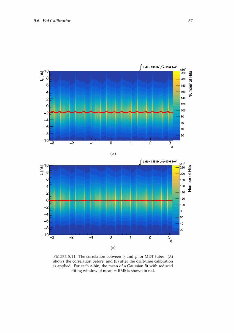
5.6. Phi Calibration 57
(A)
(B)
FIGURE 5.11: The correlation between t0 and φ for MDT tubes. (A)shows the correlation before, and (B) after the drift-time calibrationis applied. For each φ-bin, the mean of a Gaussian fit with reduced
fitting window of mean ± RMS is shown in red.
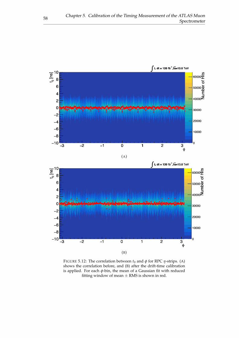
58Chapter 5. Calibration of the Timing Measurement of the ATLAS Muon
Spectrometer
(A)
(B)
FIGURE 5.12: The correlation between t0 and φ for RPC η-strips. (A)shows the correlation before, and (B) after the drift-time calibrationis applied. For each φ-bin, the mean of a Gaussian fit with reduced
fitting window of mean ± RMS is shown in red.
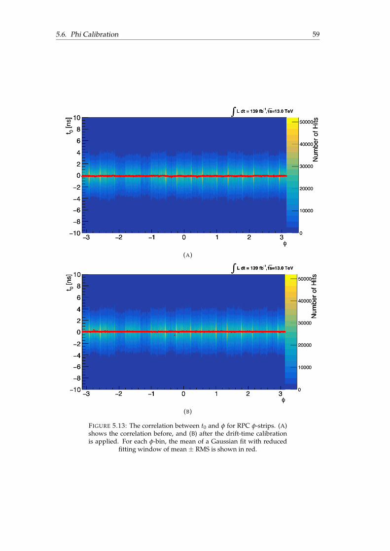
5.6. Phi Calibration 59
(A)
(B)
FIGURE 5.13: The correlation between t0 and φ for RPC φ-strips. (A)shows the correlation before, and (B) after the drift-time calibrationis applied. For each φ-bin, the mean of a Gaussian fit with reduced
fitting window of mean ± RMS is shown in red.
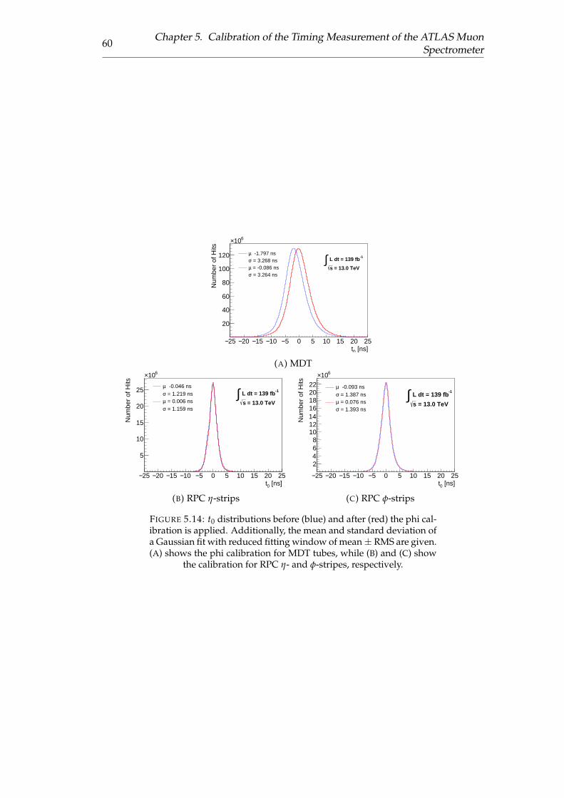
60Chapter 5. Calibration of the Timing Measurement of the ATLAS Muon
Spectrometer
25− 20− 15− 10− 5− 0 5 10 15 20 25 [ns]0t
20
40
60
80
100
120
610×
Num
ber
of H
its
-1.797 nsµ = 3.268 nsσ = -0.086 nsµ = 3.264 nsσ
-1 L dt = 139 fb∫ = 13.0 TeVs
(A) MDT
25− 20− 15− 10− 5− 0 5 10 15 20 25 [ns]0t
5
10
15
20
25
610×
Num
ber
of H
its
-0.046 nsµ = 1.219 nsσ = 0.006 nsµ = 1.159 nsσ
-1 L dt = 139 fb∫ = 13.0 TeVs
(B) RPC η-strips
25− 20− 15− 10− 5− 0 5 10 15 20 25 [ns]0t
2468
10121416182022
610×
Num
ber
of H
its
-0.093 nsµ = 1.387 nsσ = 0.076 nsµ = 1.393 nsσ
-1 L dt = 139 fb∫
= 13.0 TeVs
(C) RPC φ-strips
FIGURE 5.14: t0 distributions before (blue) and after (red) the phi cal-ibration is applied. Additionally, the mean and standard deviation ofa Gaussian fit with reduced fitting window of mean± RMS are given.(A) shows the phi calibration for MDT tubes, while (B) and (C) show
the calibration for RPC η- and φ-stripes, respectively.
5.7. Final β Resolution and Pull 61
5.7 Final β Resolution and Pull
The goal of these calibration steps was to improve the t0 measurement of each el-ement in the ATLAS MS, and thereby the distribution of the combined β measure-ment, that can be calculated according to Equation 5.5. The effect of the calibrationstrategy described in this chapter on the timing measurement of the detector systemsinvestigated in this thesis can be seen in Figure 5.15. The intention was to centre thet0 distribution around t0 = 0 ns and to decrease the width of the distribution. Forthe MDT tubes, the mean of the distribution is moved from -1.518 ns to -0.086 ns andthe standard deviation is improved from 3.552 ns to 3.264 ns. By getting rid of theshift introduced by the drift-time calibration, the mean should be pushed even fur-ther towards zero. The distribution for both RPC systems showed a spiky structuredue to the granularity of the readout system. This jagged structure can be removedby the calibration method almost entirely. Only small side-bumps remain as possi-ble remnants of the readout granularity. The distribution for RPC η-strips is pushedfrom a mean of -1.632 ns to 0.006 ns and thus is almost perfectly centred around zero.The standard deviation is reduced from 1.872 ns to 1.159 ns, and the general shapedoes comply with a Gaussian significantly better after the calibration is applied. Forthe RPC φ-strips, the mean is shifted from -2.249 ns to 0.076 ns and the standarddeviation lowered from 2.918 ns to 1.393 ns and similarly to the distribution of theRPC η-strips, the t0 distribution resembles a Gaussian significantly better after thecalibration is performed.
The effect of this calibration process on the combined β measurement can be seenin Figure 5.16, and shows a clear improvement for every detector system. For allthree detector systems, the mean of the distribution is pushed significantly closer to-wards β = 1, and the width is reduced. For the MDT tubes, the standard deviationis reduced from 0.03 to 0.027, for RPC η-stripes from 0.042 to 0.028 and for RPC φ-stripes from 0.061 to 0.031. The bigger improvements for the RPC systems are mostlikely attributed to the dissolving of the spiky nature of the t0 distributions comingfrom the readout granularity.
Before the measurements of the three detector systems can be combined in a mean-ingful way, it has to be assured that the σβ represents the measurement uncertaintiesaccurately. This can be done by evaluating the pull, as defined in Equation 5.6.
p :=1− β−1
iσbeta−1
i
(5.6)
If the measurement uncertainties are reflected correctly, the pull is known to be ofGaussian shape with a mean of zero and a standard deviation of one. The pull dis-tributions for the different detector systems can be seen in Figure 5.17. The Figureshows a clear deviation of a Gaussian shape with mean zero and standard deviationone. Consequently, the σβ have to be corrected according to Equation 5.7.
σcorrβ = σβ · (1 + |1− σp|) (5.7)
Rounded to the same decimal, this leads to σcorrβ being 0.027 for the MDT tubes, 0.030
for the RPC η-strips and 0.034 for the RPC φ-strips, which is an improvement com-pared to the uncalibrated data.
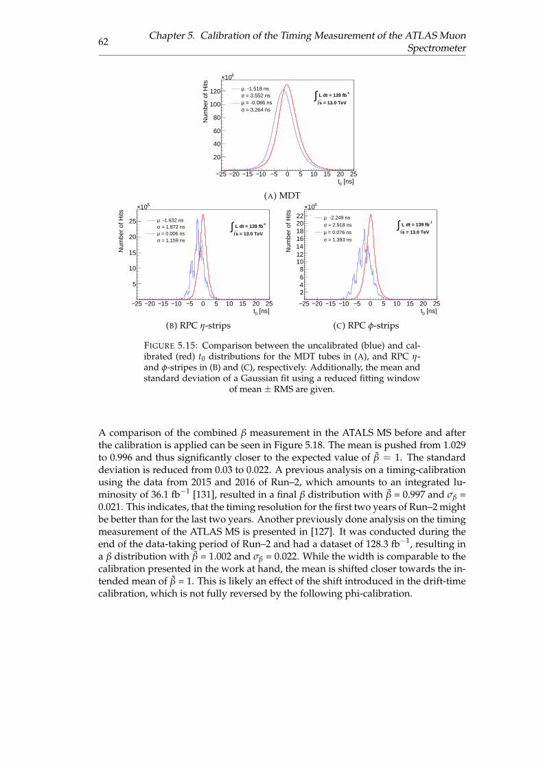
62Chapter 5. Calibration of the Timing Measurement of the ATLAS Muon
Spectrometer
25− 20− 15− 10− 5− 0 5 10 15 20 25 [ns]0t
20
40
60
80
100
120
610×
Num
ber
of H
its
-1.518 nsµ = 3.552 nsσ = -0.086 nsµ = 3.264 nsσ
-1 L dt = 139 fb∫
= 13.0 TeVs
(A) MDT
25− 20− 15− 10− 5− 0 5 10 15 20 25 [ns]0t
5
10
15
20
25
610×
Num
ber
of H
its
-1.632 nsµ = 1.872 nsσ = 0.006 nsµ = 1.159 nsσ
-1 L dt = 139 fb∫
= 13.0 TeVs
(B) RPC η-strips
25− 20− 15− 10− 5− 0 5 10 15 20 25 [ns]0t
2468
10121416182022
610×
Num
ber
of H
its
-2.249 nsµ = 2.918 nsσ = 0.076 nsµ = 1.393 nsσ
-1 L dt = 139 fb∫
= 13.0 TeVs
(C) RPC φ-strips
FIGURE 5.15: Comparison between the uncalibrated (blue) and cal-ibrated (red) t0 distributions for the MDT tubes in (A), and RPC η-and φ-stripes in (B) and (C), respectively. Additionally, the mean andstandard deviation of a Gaussian fit using a reduced fitting window
of mean ± RMS are given.
A comparison of the combined β measurement in the ATALS MS before and afterthe calibration is applied can be seen in Figure 5.18. The mean is pushed from 1.029to 0.996 and thus significantly closer to the expected value of β = 1. The standarddeviation is reduced from 0.03 to 0.022. A previous analysis on a timing-calibrationusing the data from 2015 and 2016 of Run–2, which amounts to an integrated lu-minosity of 36.1 fb−1 [131], resulted in a final β distribution with β = 0.997 and σβ =0.021. This indicates, that the timing resolution for the first two years of Run–2 mightbe better than for the last two years. Another previously done analysis on the timingmeasurement of the ATLAS MS is presented in [127]. It was conducted during theend of the data-taking period of Run–2 and had a dataset of 128.3 fb−1, resulting ina β distribution with β = 1.002 and σβ = 0.022. While the width is comparable to thecalibration presented in the work at hand, the mean is shifted closer towards the in-tended mean of β = 1. This is likely an effect of the shift introduced in the drift-timecalibration, which is not fully reversed by the following phi-calibration.
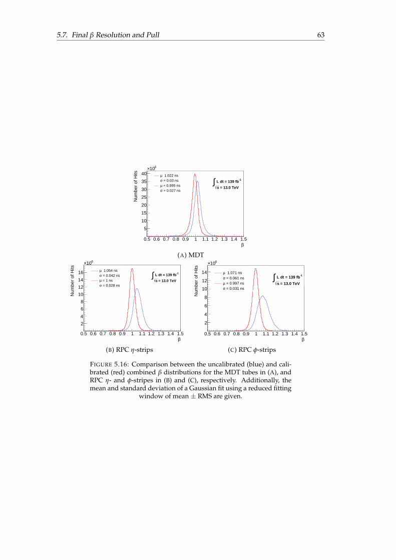
5.7. Final β Resolution and Pull 63
0.5 0.6 0.7 0.8 0.9 1 1.1 1.2 1.3 1.4 1.5β
5
10
15
20
25
30
35
40
610×
Num
ber
of H
its 1.022 nsµ = 0.03 nsσ = 0.995 nsµ = 0.027 nsσ
-1 L dt = 139 fb∫ = 13.0 TeVs
(A) MDT
0.5 0.6 0.7 0.8 0.9 1 1.1 1.2 1.3 1.4 1.5β
2
4
6
8
10
12
14
16
610×
Num
ber
of H
its 1.054 nsµ = 0.042 nsσ = 1 nsµ = 0.028 nsσ
-1 L dt = 139 fb∫ = 13.0 TeVs
(B) RPC η-strips
0.5 0.6 0.7 0.8 0.9 1 1.1 1.2 1.3 1.4 1.5β
2
4
6
8
10
12
14
610×
Num
ber
of H
its
1.071 nsµ = 0.061 nsσ = 0.997 nsµ = 0.031 nsσ
-1 L dt = 139 fb∫ = 13.0 TeVs
(C) RPC φ-strips
FIGURE 5.16: Comparison between the uncalibrated (blue) and cali-brated (red) combined β distributions for the MDT tubes in (A), andRPC η- and φ-stripes in (B) and (C), respectively. Additionally, themean and standard deviation of a Gaussian fit using a reduced fitting
window of mean ± RMS are given.
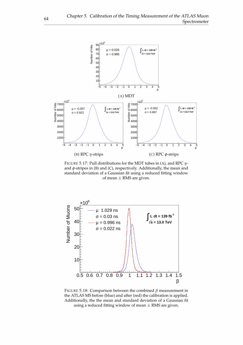
64Chapter 5. Calibration of the Timing Measurement of the ATLAS Muon
Spectrometer
5− 4− 3− 2− 1− 0 1 2 3 4 5p
10
20
30
40
50
60
70
80
90610×
Num
ber
of H
its
= 0.026µ = 0.985σ
-1 L dt = 139 fb∫ = 13.0 TeVs
(A) MDT
5− 4− 3− 2− 1− 0 1 2 3 4 5p
1000
2000
3000
4000
5000
6000
7000310×
Num
ber
of H
its
= -0.007µ = 0.922σ
-1 L dt = 139 fb∫
= 13.0 TeVs
(B) RPC η-strips
5− 4− 3− 2− 1− 0 1 2 3 4 5p
1000
2000
3000
4000
5000
6000
7000310×
Num
ber
of H
its
= -0.052µ = 0.897σ
-1 L dt = 139 fb∫ = 13.0 TeVs
(C) RPC φ-strips
FIGURE 5.17: Pull distributions for the MDT tubes in (A), and RPC η-and φ-stripes in (B) and (C), respectively. Additionally, the mean andstandard deviation of a Gaussian fit using a reduced fitting window
of mean ± RMS are given.
0.5 0.6 0.7 0.8 0.9 1 1.1 1.2 1.3 1.4 1.5β
10
20
30
40
50
610×
Num
ber
of M
uons 1.029 nsµ
= 0.03 nsσ = 0.996 nsµ = 0.022 nsσ
-1 L dt = 139 fb∫ = 13.0 TeVs
FIGURE 5.18: Comparison between the combined β measurement inthe ATLAS MS before (blue) and after (red) the calibration is applied.Additionally, the the mean and standard deviation of a Gaussian fit
using a reduced fitting window of mean ± RMS are given.
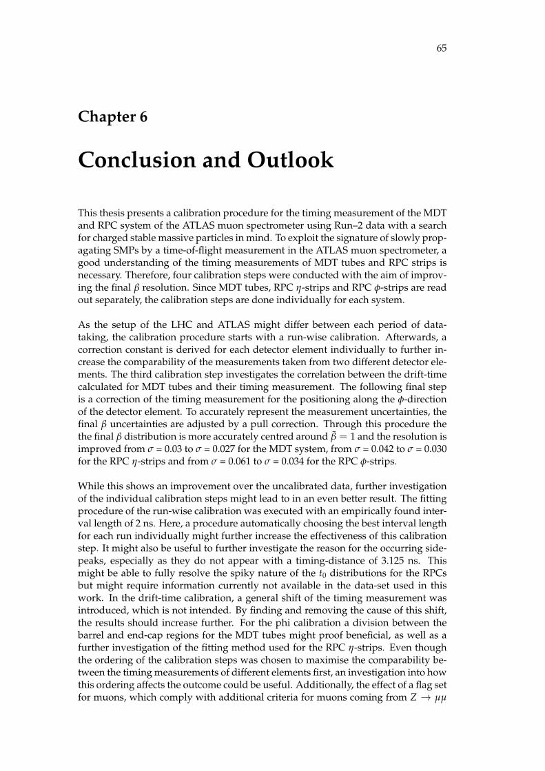
65
Chapter 6
Conclusion and Outlook
This thesis presents a calibration procedure for the timing measurement of the MDTand RPC system of the ATLAS muon spectrometer using Run–2 data with a searchfor charged stable massive particles in mind. To exploit the signature of slowly prop-agating SMPs by a time-of-flight measurement in the ATLAS muon spectrometer, agood understanding of the timing measurements of MDT tubes and RPC strips isnecessary. Therefore, four calibration steps were conducted with the aim of improv-ing the final β resolution. Since MDT tubes, RPC η-strips and RPC φ-strips are readout separately, the calibration steps are done individually for each system.
As the setup of the LHC and ATLAS might differ between each period of data-taking, the calibration procedure starts with a run-wise calibration. Afterwards, acorrection constant is derived for each detector element individually to further in-crease the comparability of the measurements taken from two different detector ele-ments. The third calibration step investigates the correlation between the drift-timecalculated for MDT tubes and their timing measurement. The following final stepis a correction of the timing measurement for the positioning along the φ-directionof the detector element. To accurately represent the measurement uncertainties, thefinal β uncertainties are adjusted by a pull correction. Through this procedure thethe final β distribution is more accurately centred around β = 1 and the resolution isimproved from σ = 0.03 to σ = 0.027 for the MDT system, from σ = 0.042 to σ = 0.030for the RPC η-strips and from σ = 0.061 to σ = 0.034 for the RPC φ-strips.
While this shows an improvement over the uncalibrated data, further investigationof the individual calibration steps might lead to in an even better result. The fittingprocedure of the run-wise calibration was executed with an empirically found inter-val length of 2 ns. Here, a procedure automatically choosing the best interval lengthfor each run individually might further increase the effectiveness of this calibrationstep. It might also be useful to further investigate the reason for the occurring side-peaks, especially as they do not appear with a timing-distance of 3.125 ns. Thismight be able to fully resolve the spiky nature of the t0 distributions for the RPCsbut might require information currently not available in the data-set used in thiswork. In the drift-time calibration, a general shift of the timing measurement wasintroduced, which is not intended. By finding and removing the cause of this shift,the results should increase further. For the phi calibration a division between thebarrel and end-cap regions for the MDT tubes might proof beneficial, as well as afurther investigation of the fitting method used for the RPC η-strips. Even thoughthe ordering of the calibration steps was chosen to maximise the comparability be-tween the timing measurements of different elements first, an investigation into howthis ordering affects the outcome could be useful. Additionally, the effect of a flag setfor muons, which comply with additional criteria for muons coming from Z → µµ

66 Chapter 6. Conclusion and Outlook
decays, could effect the outcome of the calibration. As it reduces the available statis-tics, this needs to be looked at for each calibration step individually.
Since searches for charged stable massive particles require Monte Carlo simulatedevents, the calibration must also be applied to simulated events and it must be as-sured that the t0 and β distributions for the simulated events match those of the realdata before a search for charged stable massive particles with the Run–2 data of theATLAS detector can be conducted. Additionally, it is useful to combine the timinginformation of the MS with the timing measurement of the tile calorimeter. A cal-ibration of the timing measurement in the tile calorimeter is currently in progress.When this is done, a search for charges stable massive particles can be done withthe full dataset of 139 fb−1 taken during Run–2 at
√s = 13 TeV. Such a search should
be able to either provide even stronger model-independent exclusion limits on theproduction cross-section for charged stable massive particles or be able to observethem directly and thus prove the existence of physics beyond the Standard Model.
67
Bibliography
[1] ATLAS Collaboration. “Observation of a new particle in the search for theStandard Model Higgs boson with the ATLAS detector at the LHC.” In: Phys.Lett. B 716.arXiv:1207.7214. CERN-PH-EP-2012-218 (Aug. 2012), 1–29. 29 p.DOI: 10.1016/j.physletb.2012.08.020. URL: https://cds.cern.ch/record/1471031.
[2] CMS Collaboration. “Observation of a new boson at a mass of 125 GeV withthe CMS experiment at the LHC.” In: Phys. Lett. B 716.CMS-HIG-12-028. CMS-HIG-12-028. CERN-PH-EP-2012-220 (July 2012), 30–61. 32 p. DOI: 10.1016/j.physletb.2012.08.021. URL: https://cds.cern.ch/record/1471016.
[3] D. J. Griffiths. Introduction to elementary particles; 2nd rev. version. Physics text-book. New York, NY: Wiley, 2008. URL: https://cds.cern.ch/record/111880.
[4] Guido A. Collider Physics within the Standard Model: a Primer. 2013. arXiv:1303.2842 [hep-ph].
[5] Particle Data Group. “Review of Particle Physics, 2014-2015.” In: Chin. Phys. C38 (2014). All tables, listings, and reviews (and errata) are also available on theParticle Data Group website: http://pdg.lbl.gov, p. 090001. DOI: 10.1088/1674-1137/38/9/090001. URL: https://cds.cern.ch/record/1753419.
[6] V. Martin. Particle Physics Lecture Slides. 2013. URL: https://www2.ph.ed.ac.uk/~vjm/Lectures/SH_IM_Particle_Physics_2013_files/ParticlePhysics2013Notes.pdf (visited on 07/22/2020).
[7] H. Nishino et al. “Search for Proton Decay via p → e+π0 and p → µ+π0 ina Large Water Cherenkov Detector”. In: Phys. Rev. Lett. 102 (14 Apr. 2009),p. 141801. DOI: 10.1103/PhysRevLett.102.141801. URL: https://link.aps.org/doi/10.1103/PhysRevLett.102.141801.
[8] J. Beringer et al. “Review of Particle Physics”. In: Phys. Rev. D 86 (1 July 2012),p. 010001. DOI: 10.1103/PhysRevD.86.010001. URL: https://link.aps.org/doi/10.1103/PhysRevD.86.010001.
[9] S.L. Glashow, J. Iliopoulos, and L. Maiani. “Weak Interactions with Lepton-Hadron Symmetry”. In: Phys. Rev. D 2 (1970), pp. 1285–1292. DOI: 10.1103/PhysRevD.2.1285.
[10] M. Kobayashi and T. Maskawa. “CP Violation in the Renormalizable Theoryof Weak Interaction”. In: Prog. Theor. Phys. 49 (1973), pp. 652–657. DOI: 10.1143/PTP.49.652.
[11] S. Weinberg. “A Model of Leptons”. In: Phys. Rev. Lett. 19 (1967), pp. 1264–1266. DOI: 10.1103/PhysRevLett.19.1264.
[12] P. W. Higgs. “Broken Symmetries and the Masses of Gauge Bosons”. In: Phys.Rev. Lett. 13 (1964). Ed. by J.C. Taylor, pp. 508–509. DOI: 10.1103/PhysRevLett.13.508.
68 BIBLIOGRAPHY
[13] B. Aharmim et al. “Electron energy spectra, fluxes, and day-night asymme-tries of B-8 solar neutrinos from measurements with NaCl dissolved in theheavy-water detector at the Sudbury Neutrino Observatory”. In: Phys. Rev.C 72 (2005), p. 055502. DOI: 10.1103/PhysRevC.72.055502. arXiv: nucl-ex/0502021.
[14] M. Tanabashi et al. “Review of Particle Physics”. In: Phys. Rev. D 98 (3 Aug.2018), p. 030001. DOI: 10.1103/PhysRevD.98.030001. URL: https://link.aps.org/doi/10.1103/PhysRevD.98.030001.
[15] A. O. Sushkov, W. J. Kim, D. A. R. Dalvit, and S. K. Lamoreaux. “New Ex-perimental Limits on Non-Newtonian Forces in the Micrometer Range”. In:Physical Review Letters 107.17 (Oct. 2011). ISSN: 1079-7114. DOI: 10 . 1103 /physrevlett.107.171101. URL: http://dx.doi.org/10.1103/PhysRevLett.107.171101.
[16] D. Croon, T. E. Gonzalo, L. Graf, N. Košnik, and G. White. “GUT Physics inthe Era of the LHC”. In: Frontiers in Physics 7 (June 2019). ISSN: 2296-424X.DOI: 10.3389/fphy.2019.00076. URL: http://dx.doi.org/10.3389/fphy.2019.00076.
[17] E. Corbelli and P. Salucci. “The extended rotation curve and the dark matterhalo of M33”. In: Monthly Notices of the Royal Astronomical Society 311.2 (2000),pp. 441–447. DOI: 10.1046/j.1365-8711.2000.03075.x. eprint: https://onlinelibrary.wiley.com/doi/pdf/10.1046/j.1365-8711.2000.03075.x.URL: https://onlinelibrary.wiley.com/doi/abs/10.1046/j.1365-8711.2000.03075.x.
[18] S.M. Faber and R.E. Jackson. “Velocity dispersions and mass to light ratios forelliptical galaxies”. In: Astrophys. J. 204 (1976), p. 668. DOI: 10.1086/154215.
[19] X.-P. Wu, T. Chiueh, L.-Z. Fang, and Y.-J. Xue. “A comparison of differentcluster mass estimates: consistency or discrepancy?” In: Monthly Notices of theRoyal Astronomical Society 301.3 (1998), pp. 861–871. DOI: 10.1046/j.1365-8711.1998.02055.x. eprint: https://onlinelibrary.wiley.com/doi/pdf/10.1046/j.1365-8711.1998.02055.x. URL: https://onlinelibrary.wiley.com/doi/abs/10.1046/j.1365-8711.1998.02055.x.
[20] C.S. Frenk and S.D.M. White. “Dark matter and cosmic structure”. In: An-nalen der Physik 524.9-10 (2012), pp. 507–534. DOI: 10.1002/andp.201200212.eprint: https : / / onlinelibrary . wiley . com / doi / pdf / 10 . 1002 / andp .201200212. URL: https://onlinelibrary.wiley.com/doi/abs/10.1002/andp.201200212.
[21] Planck Collaboration. “Planck 2013 results. I. Overview of products and sci-entific results”. In: A&A 571 (2014), A1. DOI: 10.1051/0004-6361/201321529.URL: https://doi.org/10.1051/0004-6361/201321529.
[22] L. Bergström. “Non-baryonic dark matter: Observational evidence and de-tection methods”. In: Reports on Progress in Physics 63 (May 2000), p. 793. DOI:10.1088/0034-4885/63/5/2r3.
[23] M.B. Gavela, P. Hernandez, J. Orloff, and O. Pene. “Standard model CP vio-lation and baryon asymmetry”. In: Mod. Phys. Lett. A 9 (1994), pp. 795–810.DOI: 10.1142/S0217732394000629. arXiv: hep-ph/9312215.
BIBLIOGRAPHY 69
[24] M.B. Gavela, P. Hernandez, J. Orloff, O. Pene, and C. Quimbay. “Standardmodel CP violation and baryon asymmetry. Part 2: Finite temperature”. In:Nucl. Phys. B 430 (1994), pp. 382–426. DOI: 10.1016/0550-3213(94)00410-2.arXiv: hep-ph/9406289.
[25] P. Huet and E. Sather. “Electroweak baryogenesis and standard model CPviolation”. In: Phys. Rev. D 51 (1995), pp. 379–394. DOI: 10.1103/PhysRevD.51.379. arXiv: hep-ph/9404302.
[26] K. G. Wilson. “The Renormalization Group and Strong Interactions”. In: Phys.Rev. D 3 (1971), p. 1818. DOI: 10.1103/PhysRevD.3.1818.
[27] M. Dine. “Naturalness Under Stress”. In: Ann. Rev. Nucl. Part. Sci. 65 (2015),pp. 43–62. DOI: 10.1146/annurev-nucl-102014-022053. arXiv: 1501.01035[hep-ph].
[28] Gerard ’t Hooft, C. Itzykson, A. Jaffe, H. Lehmann, P.K. Mitter, I.M. Singer,and R. Stora, eds. Recent Developments in Gauge Theories. Proceedings, Nato Ad-vanced Study Institute, Cargese, France, August 26 - September 8, 1979. Vol. 59.1980, pp.1–438. DOI: 10.1007/978-1-4684-7571-5.
[29] L. Susskind. “Dynamics of Spontaneous Symmetry Breaking in the Weinberg-Salam Theory”. In: Phys. Rev. D 20 (1979), pp. 2619–2625. DOI: 10 . 1103 /PhysRevD.20.2619.
[30] Y. A Gelfand and E. P. Likhtman. “Extension of the algebra of Poincare groupgenerators and violation of P invariance”. In: JETP Lett. 13.8 (1971), pp. 323–325. URL: http://cds.cern.ch/record/433516.
[31] D.V. Volkov and V.P. Akulov. “Is the Neutrino a Goldstone Particle?” In: Phys.Lett. B 46 (1973), pp. 109–110. DOI: 10.1016/0370-2693(73)90490-5.
[32] J. Wess and B. Zumino. “Supergauge transformations in four dimensions”.In: Nucl. Phys. B 70.CERN-TH-1753. 1 (1974), pp. 39–50. DOI: 10.1016/0550-3213(74)90355-1. URL: https://cds.cern.ch/record/201649.
[33] J. Wess and B. Zumino. “Supergauge Invariant Extension of Quantum Elec-trodynamics”. In: Nucl. Phys. B 78 (1974), p. 1. DOI: 10.1016/0550-3213(74)90112-6.
[34] S. Ferrara and B. Zumino. “Supergauge Invariant Yang-Mills Theories”. In:Nucl. Phys. B 79 (1974), p. 413. DOI: 10.1016/0550-3213(74)90559-8.
[35] A. Salam and J.A. Strathdee. “Supersymmetry and Nonabelian Gauges”. In:Phys. Lett. B 51 (1974), pp. 353–355. DOI: 10.1016/0370-2693(74)90226-3.
[36] N. Sakai. “Naturalness in Supersymmetric Guts”. In: Z. Phys. C 11 (1981),p. 153. DOI: 10.1007/BF01573998.
[37] S. Dimopoulos, S. Raby, and F. Wilczek. “Supersymmetry and the Scale ofUnification”. In: Phys. Rev. D 24 (1981), pp. 1681–1683. DOI: 10.1103/PhysRevD.24.1681.
[38] L. E. Ibanez and G. G. Ross. “Low-Energy Predictions in SupersymmetricGrand Unified Theories”. In: Phys. Lett. B 105 (1981), pp. 439–442. DOI: 10.1016/0370-2693(81)91200-4.
[39] S. Dimopoulos and H. Georgi. “Softly Broken Supersymmetry and SU(5)”. In:Nucl. Phys. B 193 (1981), pp. 150–162. DOI: 10.1016/0550-3213(81)90522-8.
[40] H. Goldberg. “Constraint on the Photino Mass from Cosmology”. In: Phys.Rev. Lett. 50 (1983). Ed. by M.A. Srednicki. [Erratum: Phys.Rev.Lett. 103, 099905(2009)], p. 1419. DOI: 10.1103/PhysRevLett.50.1419.
70 BIBLIOGRAPHY
[41] J. R. Ellis, J.S. Hagelin, D. V. Nanopoulos, K. A. Olive, and M. Srednicki. “Su-persymmetric Relics from the Big Bang”. In: Nucl. Phys. B 238 (1984). Ed. byM.A. Srednicki, pp. 453–476. DOI: 10.1016/0550-3213(84)90461-9.
[42] S. P. Martin. “A Supersymmetry primer”. In: Perspectives on supersymmetry.Vol.2. Ed. by Gordon L. Kane. Vol. 21. 2010, pp. 1–153. DOI: 10.1142/9789812839657\_0001. arXiv: hep-ph/9709356.
[43] M. Dine. Supersymmetry and String Theory: Beyond the Standard Model. Cam-bridge University Press, 2007. DOI: 10.1017/CBO9780511618482.
[44] J. A. Bagger. “Weak scale supersymmetry: Theory and practice”. In: Theoreti-cal Advanced Study Institute in Elementary Particle Physics (TASI 95): QCD andBeyond. Apr. 1996, pp. 109–162. arXiv: hep-ph/9604232.
[45] I. J.R. Aitchison. “Supersymmetry and the MSSM: An Elementary introduc-tion”. In: (May 2005). arXiv: hep-ph/0505105.
[46] G. R. Farrar and P. Fayet. “Phenomenology of the Production, Decay, and De-tection of New Hadronic States Associated with Supersymmetry”. In: Phys.Lett. B 76 (1978), pp. 575–579. DOI: 10.1016/0370-2693(78)90858-4.
[47] L. E. Ibáñez and G. G. Ross. “Discrete gauge symmetries and the origin ofbaryon and lepton number conservation in supersymmetric versions of thestandard model”. In: Nucl. Phys. B 368.CERN-TH-6111-91 (1992), pp. 3–37.DOI: 10.1016/0550-3213(92)90195-H. URL: http://cds.cern.ch/record/245866.
[48] S. Weinberg. “Supersymmetry at Ordinary Energies. 1. Masses and Conserva-tion Laws”. In: Phys. Rev. D 26 (1982), p. 287. DOI: 10.1103/PhysRevD.26.287.
[49] N. Sakai and T. Yanagida. “Proton Decay in a Class of Supersymmetric GrandUnified Models”. In: Nucl. Phys. B 197 (1982), p. 533. DOI: 10.1016/0550-3213(82)90457-6.
[50] M. Lisanti. “Lectures on Dark Matter Physics”. In: Theoretical Advanced StudyInstitute in Elementary Particle Physics: New Frontiers in Fields and Strings. 2017,pp. 399–446. DOI: 10.1142/9789813149441\_0007. arXiv: 1603.03797 [hep-ph].
[51] L. Randall and R. Sundrum. “A Large mass hierarchy from a small extra di-mension”. In: Phys. Rev. Lett. 83 (1999), pp. 3370–3373. DOI: 10.1103/PhysRevLett.83.3370. arXiv: hep-ph/9905221.
[52] L. Randall and R. Sundrum. “An Alternative to compactification”. In: Phys.Rev. Lett. 83 (1999), pp. 4690–4693. DOI: 10.1103/PhysRevLett.83.4690.arXiv: hep-th/9906064.
[53] C. F. Kolda. “Gauge mediated supersymmetry breaking: Introduction, reviewand update”. In: Nucl. Phys. B Proc. Suppl. 62 (1998). Ed. by M. Cvetic and P.Langacker, pp. 266–275. DOI: 10.1016/S0920-5632(97)00667-1. arXiv: hep-ph/9707450.
[54] L. Randall and R. Sundrum. “Out of this world supersymmetry breaking”. In:Nucl. Phys. B 557 (1999), pp. 79–118. DOI: 10.1016/S0550-3213(99)00359-4.arXiv: hep-th/9810155.
[55] A. Pomarol and R. Rattazzi. “Sparticle masses from the superconformal anomaly”.In: JHEP 05 (1999), p. 013. DOI: 10.1088/1126-6708/1999/05/013. arXiv:hep-ph/9903448.
BIBLIOGRAPHY 71
[56] A. H. Chamseddine, R. Arnowitt, and Pran Nath. “Locally SupersymmetricGrand Unification”. In: Phys. Rev. Lett. 49 (14 Oct. 1982), pp. 970–974. DOI:10.1103/PhysRevLett.49.970. URL: https://link.aps.org/doi/10.1103/PhysRevLett.49.970.
[57] R. Arnowitt and P. Nath. “Developments in Supergravity Unified Models”.In: Perspectives on supersymmetry. Vol.2. Ed. by Gordon L. Kane. Vol. 21. 2010,pp. 222–243. DOI: 10.1142/9789814307505\_0003. arXiv: 0912.2273 [hep-ph].
[58] R. Barbieri and G. F. Giudice. “Upper bounds on supersymmetric particlemasses”. In: Nucl. Phys. B 306.CERN-TH-4825-87 (Aug. 1987), 63–76. 19 p.DOI: 10.1016/0550-3213(88)90171-X. URL: https://cds.cern.ch/record/180560.
[59] B. de Carlos and J.A. Casas. “One-loop analysis of the electroweak break-ing in supersymmetric models and the fine-tuning problem”. In: Phys. Lett.B 309.hep-ph/9303291. CERN-TH-6835-93. IEM-FT-70 (Mar. 1993), 320–328.16 p. DOI: 10.1016/0370-2693(93)90940-J. URL: http://cds.cern.ch/record/247620.
[60] ATLAS Collaboration. “Summary of the searches for squarks and gluinos us-ing√
s = 8 TeV pp collisions with the ATLAS experiment at the LHC”. In:JHEP 10 (2015), p. 054. DOI: 10.1007/JHEP10(2015)054. arXiv: 1507.05525[hep-ex].
[61] ATLAS Collaboration. “Search for electroweak production of supersymmet-ric particles in final states with two or three leptons at
√s = 13 TeV with the
ATLAS detector”. In: Eur. Phys. J. C 78.12 (2018), p. 995. DOI: 10.1140/epjc/s10052-018-6423-7. arXiv: 1803.02762 [hep-ex].
[62] ATLAS Collaboration. “Summary of the ATLAS experiment’s sensitivity tosupersymmetry after LHC Run 1 — interpreted in the phenomenologicalMSSM”. In: JHEP 10 (2015), p. 134. DOI: 10.1007/JHEP10(2015)134. arXiv:1508.06608 [hep-ex].
[63] H. Baer, V. Barger, J. S. Gainer, P. Huang, M. Savoy, H. Serce, and X. Tata.“What hadron collider is required to discover or falsify natural supersymme-try?” In: Phys. Lett. B 774 (2017), pp. 451–455. DOI: 10.1016/j.physletb.2017.09.086. arXiv: 1702.06588 [hep-ph].
[64] S. Rappoccio. “The experimental status of direct searches for exotic physicsbeyond the standard model at the Large Hadron Collider”. In: Rev. Phys. 4(2019), p. 100027. DOI: 10.1016/j.revip.2018.100027. arXiv: 1810.10579[hep-ex].
[65] S. Diglio, L. Feligioni, and G. Moultaka. “Stashing the stops in multijet eventsat the LHC”. In: Phys. Rev. D 96.5 (2017), p. 055032. DOI: 10.1103/PhysRevD.96.055032. arXiv: 1611.05850 [hep-ph].
[66] T. Flacke, D. W. Kang, K. Kong, G. Mohlabeng, and S. C. Park. “ElectroweakKaluza-Klein Dark Matter”. In: JHEP 04 (2017), p. 041. DOI: 10.1007/JHEP04(2017)041. arXiv: 1702.02949 [hep-ph].
[67] M. Fairbairn, A.C. Kraan, D.A. Milstead, T. Sjostrand, Peter Z. Skands, andT. Sloan. “Stable Massive Particles at Colliders”. In: Phys. Rept. 438 (2007),pp. 1–63. DOI: 10.1016/j.physrep.2006.10.002. arXiv: hep-ph/0611040.
[68] H. Baer, K. Cheung, and J. F. Gunion. “A Heavy gluino as the lightest su-persymmetric particle”. In: Phys. Rev. D 59 (1999), p. 075002. DOI: 10.1103/PhysRevD.59.075002. arXiv: hep-ph/9806361.
72 BIBLIOGRAPHY
[69] R. Barbier et al. “R-parity violating supersymmetry”. In: Phys. Rept. 420 (2005),pp. 1–202. DOI: 10.1016/j.physrep.2005.08.006. arXiv: hep-ph/0406039.
[70] H. K. Dreiner. “An Introduction to explicit R-parity violation”. In: Perspectiveson supersymmetry. Vol.2. Ed. by Gordon L. Kane. Vol. 21. 2010, pp. 565–583.DOI: 10.1142/9789814307505\_0017. arXiv: hep-ph/9707435.
[71] ATLAS Collaboration. “Search for heavy charged long-lived particles in theATLAS detector in 36.1 fb−1 of proton-proton collision data at
√s = 13 TeV”.
In: Phys. Rev. D 99.arXiv:1902.01636 (Feb. 2019), 092007. 34 p. DOI: 10.1103/PhysRevD.99.092007. URL: https://cds.cern.ch/record/2655808.
[72] CERN. Our Member States. 2020. URL: https://home.cern/about/who-we-are/our-governance/member-states (visited on 07/14/2020).
[73] “About CERN”. In: (Jan. 2012). URL: http://cds.cern.ch/record/1997225.
[74] L. R Evans and P. Bryant. “LHC Machine”. In: JINST 3 (2008). This reportis an abridged version of the LHC Design Report (CERN-2004-003), S08001.164 p. DOI: 10.1088/1748-0221/3/08/S08001. URL: http://cds.cern.ch/record/1129806.
[75] ATLAS Collaboration. “The ATLAS Experiment at the CERN Large HadronCollider”. In: JINST 3 (2008). Also published by CERN Geneva in 2010, S08003.437 p. DOI: 10.1088/1748-0221/3/08/S08003. URL: https://cds.cern.ch/record/1129811.
[76] LEP design report. By the LEP Injector Study Group. Geneva: CERN, 1983.URL: https://cds.cern.ch/record/98881.
[77] LEP design report. Copies shelved as reports in LEP, PS and SPS libraries.Geneva: CERN, 1984. URL: https://cds.cern.ch/record/102083.
[78] C. Wyss. LEP design report, v.3: LEP2. Vol. 1-2 publ. in 1983-84. Geneva: CERN,1996. URL: https://cds.cern.ch/record/314187.
[79] N. Grau. The Heavy Ion Physics Program with ATLAS at the LHC. 2007. arXiv:0706.1983 [nucl-ex].
[80] V. Shiltsev and F. Zimmermann. Modern and Future Colliders. 2020. arXiv:2003.09084 [physics.acc-ph].
[81] CERN. Facts and figures about the LHC. 2020. URL: https : / / home . cern /resources/faqs/facts-and-figures-about-lhc (visited on 07/14/2020).
[82] ALICE Collaboration. “The ALICE experiment at the CERN LHC”. In: JINST3 (2008), S08002. DOI: 10.1088/1748-0221/3/08/S08002.
[83] CMS Collaboration. “The CMS Experiment at the CERN LHC”. In: JINST 3(2008), S08004. DOI: 10.1088/1748-0221/3/08/S08004.
[84] LHCb Collaboration. “The LHCb Detector at the LHC”. In: JINST 3 (2008),S08005. DOI: 10.1088/1748-0221/3/08/S08005.
[85] E. Mobs. “The CERN accelerator complex. Complexe des accélérateurs duCERN”. In: (July 2016). General Photo. URL: https://cds.cern.ch/record/2197559.
[86] CERN. CERN’s accelerator complex. 2020. URL: https://home.cern/science/accelerators/accelerator-complex (visited on 07/14/2020).

BIBLIOGRAPHY 73
[87] ATLAS Collaboration. “ATLAS Run 1 searches for direct pair production ofthird-generation squarks at the Large Hadron Collider”. In: The EuropeanPhysical Journal C 75.10 (Oct. 2015). ISSN: 1434-6052. DOI: 10.1140/epjc/s10052-015-3726-9. URL: http://dx.doi.org/10.1140/epjc/s10052-015-3726-9.
[88] ATLAS Collaboration. “ATLAS data quality operations and performance for2015–2018 data-taking”. In: Journal of Instrumentation 15.04 (Apr. 2020), P04003–P04003. ISSN: 1748-0221. DOI: 10.1088/1748-0221/15/04/p04003. URL: http://dx.doi.org/10.1088/1748-0221/15/04/P04003.
[89] CERN. Record luminosity: well done LHC. 2020. URL: https://home.cern/news/news/accelerators/record-luminosity-well-done-lhc (visited on07/16/2020).
[90] ATLAS Collaboration. Luminosity Public Results Run 2. 2020. URL: https://twiki.cern.ch/twiki/bin/view/AtlasPublic/LuminosityPublicResultsRun2#2015_pp_Collisions (visited on 07/16/2020).
[91] ATLAS Collaboration. Detector - Magnet System. 2020. URL: https://atlas.cern/discover/detector/magnet-system (visited on 07/17/2020).
[92] J. Pequenao and P. Schaffner. “How ATLAS detects particles: diagram of par-ticle paths in the detector”. Jan. 2013. URL: https://cds.cern.ch/record/1505342.
[93] U. Egede. “The search for a Standard Model Higgs at the LHC and electronidentification using transition radiation in the ATLAS tracker”. PhD thesis.Lund U., 1998.
[94] Yiming Abulaiti. “Search for Pair-Produced Supersymmetric Top Quark Part-ners with the ATLAS Experiment”. PhD thesis. Stockholm U., Aug. 2016.
[95] R. E. Owen. “The ATLAS Trigger System”. In: (Feb. 2018). URL: http://cds.cern.ch/record/2302730.
[96] ATLAS Collaboration. The Inner Detector. 2020. URL: https://atlas.cern/discover/detector/inner-detector (visited on 07/20/2020).
[97] K. Potamianos. “The upgraded Pixel detector and the commissioning of theInner Detector tracking of the ATLAS experiment for Run-2 at the LargeHadron Collider”. In: PoS EPS-HEP2015 (2015), p. 261. arXiv: 1608.07850[physics.ins-det].
[98] H Oide. The Pixel Detector of the ATLAS experiment for the Run 2 at the LargeHadron Collider. Tech. rep. ATL-INDET-PROC-2014-005. 12. Geneva: CERN,Sept. 2014. DOI: 10.1088/1748-0221/9/12/C12034. URL: http://cds.cern.ch/record/1757476.
[99] M. Capeans, G. Darbo, K. Einsweiller, M. Elsing, T Flick, M Garcia-Sciveres,C Gemme, H Pernegger, O Rohne, and R Vuillermet. ATLAS Insertable B-LayerTechnical Design Report. Tech. rep. CERN-LHCC-2010-013. ATLAS-TDR-19.Sept. 2010. URL: https://cds.cern.ch/record/1291633.
[100] ATLAS Collaboration. “ATLAS pixel detector electronics and sensors”. In:Journal of Instrumentation 3.07 (July 2008), P07007–P07007. DOI: 10 . 1088 /1748 - 0221 / 3 / 07 / p07007. URL: https : / / doi . org / 10 . 1088 % 2F1748 -0221%2F3%2F07%2Fp07007.
74 BIBLIOGRAPHY
[101] N. Barlow. Operation of the ATLAS Semiconductor Tracker. Tech. rep. ATL-INDET-PROC-2010-003. Geneva: CERN, Feb. 2010. URL: http : / / cds . cern . ch /record/1237401.
[102] B. Mindur. ATLAS Transition Radiation Tracker (TRT): Straw tubes for trackingand particle identification at the Large Hadron Collider. Tech. rep. ATL-INDET-PROC-2016-001. Geneva: CERN, Mar. 2016. DOI: 10.1016/j.nima.2016.04.026. URL: https://cds.cern.ch/record/2139567.
[103] ATLAS liquid-argon calorimeter: Technical Design Report. Technical Design Re-port ATLAS. Geneva: CERN, 1996. URL: https://cds.cern.ch/record/331061.
[104] ATLAS Collaboration. ATLAS tile calorimeter: Technical Design Report. Techni-cal Design Report ATLAS. Geneva: CERN, 1996. URL: https://cds.cern.ch/record/331062.
[105] N J Buchanan et al. “Design and implementation of the Front End Board forthe readout of the ATLAS liquid argon calorimeters”. In: Journal of Instrumen-tation 3.03 (Mar. 2008), P03004–P03004. DOI: 10.1088/1748- 0221/3/03/p03004. URL: https://doi.org/10.1088%2F1748-0221%2F3%2F03%2Fp03004.
[106] E. Diehl. Calibration and Performance of the ATLAS Muon Spectrometer. 2011.arXiv: 1109.6933 [physics.ins-det].
[107] ATLAS Collaboration. “Commissioning of the ATLAS Muon Spectrometerwith cosmic rays”. In: The European Physical Journal C 70.3 (Oct. 2010), pp. 875–916. ISSN: 1434-6052. DOI: 10.1140/epjc/s10052-010-1415-2. URL: http://dx.doi.org/10.1140/epjc/s10052-010-1415-2.
[108] ATLAS Collaboration. Barrel sketch. 2020. URL: https://atlas-muon-align.web.cern.ch/Plots/atlas_sketch.png (visited on 07/22/2020).
[109] J. Wotschack. ATLAS Muon Chamber Construction Parameters for CSC, MDT,and RPC chambers. Tech. rep. ATL-MUON-PUB-2008-006. ATL-COM-MUON-2008-008. Back-up document for the ATLAS Detector Paper. Geneva: CERN,Apr. 2008. URL: http://cds.cern.ch/record/1099400.
[110] ATLAS Collaboration. Expected performance of the ATLAS experiment: detec-tor, trigger and physics. Geneva: CERN, 2009. URL: https://cds.cern.ch/record/1125884.
[111] ATLAS Collaboration. ATLAS muon spectrometer: Technical Design Report. Tech-nical Design Report ATLAS. Geneva: CERN, 1997. URL: https://cds.cern.ch/record/331068.
[112] ATLAS Muon Group. Monitored drift tubes in ATLAS. 2020. URL: https://cds.cern.ch/record/319197/files/muon-96-129.pdf (visited on 07/22/2020).
[113] Y Arai et al. “ATLAS Muon Drift Tube Electronics”. In: JINST 3.ATL-MUON-PUB-2008-008. (Apr. 2008), P09001. 58 p. DOI: 10.1088/1748-0221/3/09/P09001. URL: http://cds.cern.ch/record/1100199.
[114] D Boscherini. Performance and operation of the ATLAS Resistive Plate Chambersystem in LHC Run-1. Tech. rep. ATL-MUON-PROC-2014-005. 12. Geneva:CERN, Sept. 2014. DOI: 10 . 1088 / 1748 - 0221 / 9 / 12 / C12039. URL: http ://cds.cern.ch/record/1753173.
BIBLIOGRAPHY 75
[115] A Aloisio et al. The RPC Level-1 Muon Trigger of the ATLAS Experiment at theLHC. Tech. rep. ATL-DAQ-CONF-2006-004. ATL-COM-DAQ-2006-011. Geneva:CERN, Mar. 2006. DOI: 10.1109/RTC.2005.1547462. URL: http://cds.cern.ch/record/934478.
[116] ATLAS Collaboration. “Search for heavy charged long-lived particles in proton-proton collisions at
√s = 13 TeV using an ionisation measurement with the
ATLAS detector”. In: Phys. Lett. B 788.arXiv:1808.04095 (Aug. 2018), 96–116.21 p. DOI: 10.1016/j.physletb.2018.10.055. URL: http://cds.cern.ch/record/2634050.
[117] D. C. Swift and J. M. McNaney. “Approximate, analytic solutions of the Betheequation for charged particle range”. In: (Dec. 2008). arXiv: 0901.4145 [cond-mat.other].
[118] H. Schieck. Nuclear Reactions - An Introduction. Vol. 882. Jan. 2014. ISBN: 978-3-642-53985-5. DOI: 10.1007/978-3-642-53986-2.
[119] C. Becchi and M. D’Elia. “Introduction to the Basic Concepts of Modern Physics”.In: Introduction to the Basic Concepts of Modern Physics: Special Relativity, Quan-tum and Statistical Physics, UNITEXT. ISBN 978-88-470-1615-6. Springer-VerlagMilan, 2010 (Jan. 2010). DOI: 10.1007/978-88-470-1616-3.
[120] S. Tarem, Z. Tarem, N. Panikashvili, and O. Belkind. “MuGirl – Muon iden-tification in the ATLAS detector from the inside out”. In: 2006 IEEE NuclearScience Symposium Conference Record. Vol. 1. 2006, pp. 617–621.
[121] D. Fassouliotis, T. Lagouri, A. Poppleton, S. Robins, G. D. Stavropoulos, andI. Vichou. Muon Identification using the MUID package. Tech. rep. ATL-COM-MUON-2003-003. Geneva: CERN, Nov. 2000. URL: https://cds.cern.ch/record/681596.
[122] R. Nicolaidou, L. Chevalier, S. Hassani, J.F. Laporte, E. Le Menedeu, and A.Ouraou. “Muon identification procedure for the ATLAS detector at the LHCusing Muonboy reconstruction package and tests of its performance usingcosmic rays and single beam data”. In: J. Phys. Conf. Ser. 219 (2010). Ed. byJan Gruntorad and Milos Lokajicek, p. 032052. DOI: 10.1088/1742- 6596/219/3/032052.
[123] ATLAS Collaboration. “Muon reconstruction performance of the ATLAS de-tector in proton–proton collision data at
√s =13 TeV”. In: Eur. Phys. J. C 76.5
(2016), p. 292. DOI: 10.1140/epjc/s10052-016-4120-y. arXiv: 1603.05598[hep-ex].
[124] S. Tarem, Shikma Bressler, H. Nomoto, and Alessandro Di Mattia. “Triggerand Reconstruction for a heavy long lived charged particles with the ATLASdetector”. In: European Physical Journal C 62 (July 2009), pp. 281–292. DOI: 10.1140/epjc/s10052-009-1040-0.
[125] S. Tarem, S. Bressler, H. Nomoto, and A. Di Mattia. “Trigger and reconstruc-tion for heavy long-lived charged particles with the ATLAS detector”. In: Eur.Phys. J. C 62 (2009), pp. 281–292. DOI: 10.1140/epjc/s10052-009-1040-0.
[126] S Tarem. Reconstruction And Identification Of Heavy Long-Lived Particles At TheATLAS Detector At The LHC. Tech. rep. ATL-PHYS-PROC-2009-123. Geneva:CERN, Oct. 2009. URL: http://cds.cern.ch/record/1210439.
[127] M. Habedank. “Calibrating the ATLAS Muon Spectrometer for a Search forCharged Stable Massive Particles”. MA thesis. Ludwig-Maximilians-UniversitätMünchen, Nov. 2018.
76 BIBLIOGRAPHY
[128] M. Adersberger. “Searches for Heavy Charged Long-Lived Particles with theATLAS Detector”. PhD thesis. Ludwig-Maximilians-Universität München,Nov. 2018.
[129] ATLAS Collaboration. Luminosity determination in pp collisions at√
s = 13TeV using the ATLAS detector at the LHC. Tech. rep. ATLAS-CONF-2019-021.Geneva: CERN, June 2019. URL: https://cds.cern.ch/record/2677054.
[130] J. Catmore, P. Laycock, E. Gramstad, T. Gillam, J. Cranshaw, N. Ozturk, andG. Stewart. A New Petabyte-scale Data Derivation Framework for ATLAS. Tech.rep. ATL-SOFT-PROC-2015-041. 7. Geneva: CERN, May 2015. DOI: 10.1088/1742-6596/664/7/072007. URL: https://cds.cern.ch/record/2016628.
[131] J. Heinrich. “Search for Charged Stable Massive Particles with the ATLAS De-tector”. PhD thesis. Ludwig-Maximilians-Universität München, Mar. 2018.

77
Declaration of AuthorshipHiermit erkläre ich, die vorliegende Arbeit selbstständig verfasst zu haben und keineanderen als die in der Arbeit angegebenen Quellen und Hilfsmittel benutzt zu haben.
München,
Unterschrift: