1

Tiny Transformers for Environmental SoundClassification at the Edge

David Elliott, Member, IEEE, Carlos E. Otero, Senior Member, IEEE, Steven Wyatt, Member, IEEE,Evan Martino, Member, IEEE

Abstract—With the growth of the Internet of Things and therise of Big Data, data processing and machine learning applica-tions are being moved to cheap and low size, weight, and power(SWaP) devices at the edge, often in the form of mobile phones,embedded systems, or microcontrollers. The field of Cyber-Physical Measurements and Signature Intelligence (MASINT)makes use of these devices to analyze and exploit data in waysnot otherwise possible, which results in increased data quality,increased security, and decreased bandwidth. However, methodsto train and deploy models at the edge are limited, and modelswith sufficient accuracy are often too large for the edge device.Therefore, there is a clear need for techniques to create efficientAI/ML at the edge. This work presents training techniques foraudio models in the field of environmental sound classificationat the edge. Specifically, we design and train Transformers toclassify office sounds in audio clips. Results show that a BERT-based Transformer, trained on Mel spectrograms, can outperforma CNN using 99.85% fewer parameters. To achieve this result, wefirst tested several audio feature extraction techniques designedfor Transformers, using ESC-50 for evaluation, along withvarious augmentations. Our final model outperforms the state-of-the-art MFCC-based CNN on the office sounds dataset, using justover 6,000 parameters – small enough to run on a microcontroller.

Index Terms—edge; environmental sound classification; ma-chine learning; audio; transformers; feature extraction; pretrain-ing; finetuning; self-attention

I. INTRODUCTION

THE field of environmental sound classification (ESC)has been actively researched for many years, with ap-

plications in security, surveillance, manufacturing, AVs, andmore [1]. In modern days, ESC has important applications toautonomous vehicles (AV), as they can be used to detect sirens,accidents, locations, in-cabin disturbances, and much more. Asvehicle-based computational power increases, and algorithmsimprove, it becomes vital to explore a wide number of optionsto perform a given machine learning task. For ESC, this meansexploring transformers [2] as a possible means to perform ESCat the edge.

Recent work in transformers has profoundly affected thefield of natural language processing (NLP), seeing models suchas BERT [3], XLNet [4], T5 [5], GPT [6]–[8], and BigBird[9] – to name a few – iteratively setting new state-of-the-artfor a variety of difficult NLP tasks. In many cases, transformer

D. Elliott, C. E. Otero, S. Wyatt, and E. Martino are with the Departmentof Computer Engineering and Sciences, Florida Institute of Technology,Melbourne, FL, 32901 USA e-mail: delliott2013@my.fit.edu.

This work has been submitted to the IEEE for possible publication.Copyright may be transferred without notice, after which this version mayno longer be accessible.

accuracy exceeds the performance of humans on the sametasks.

Even though most of the highly public work with transform-ers has been done in NLP, a transformer, which fundamentallyis simply a series of self-attention operations stacked on topof one another [2], is a general architecture that can beapplied to any input. OpenAI, an AI research and developmentcompany focused on ensuring artificial general intelligencebenefits humanity 1, made this clear in several of their recentworks. In ImageGPT [10], Chen et al. showed how the GPTarchitecture, which is transformer-based, can be trained inan autoregressive fashion on a wide variety of images, inorder to generate realistic image completions and samples.Notably, images were restricted to 64x64 pixels, as a greateramount of pixels requires substantially more compute than wasfeasible. In Jukebox [11], a transformer is used along withvector-quantized variational autoencoders (VQ-VAEs) [12], inorder to generate realistic audio. Also notable is the fact thatDhariwal et al. trained the transformer on a highly compressedrepresentation of the audio waveform generated by VQ-VAEs,rather than the raw waveform, and that the outputs fromthe transformer are not used directly, but are passed throughan upsampler first. Even so, the total cost of training thefull Jukebox system is in excess of 20,000 V100-days – anenormous cost [11]. More recently, in a paper under reviewat ICLR 2021, it has been found that, given enough data(hundreds of millions of examples), transformers can exceedeven the best CNNs in accuracy [13]. We take this, in additionto the recent trend in larger datasets and more compute, tomean that any work we perform here with small datasets andmodest transformers can easily be scaled up at a later date.

The field of audio speech recognition (ASR) has pickedup transformers with vigor. Indeed, it is understandable, asapplying transformers is straightforward for many approachesto ASR. Often based on encoder-decoders [14], the most obvi-ous use of a transformer is in the decoder of an ASR system,which usually has text as input and output, thus making theapplication of any state-of-the-art language models, such asBERT or its variants, available to it with little adaptationneeded. Some work [15] has also made use of a transformerin the encoder as well, thus making the ASR system an end-to-end transformer model. Recent work has seen transformersimprove the state-of-the-art for ASR by reducing word errorrate by 10% in clean speech, and 5% in more challengingspeech [16].

1https://openai.com/

arX

iv:2

103.

1215

7v1

[cs

.SD

] 2

2 M

ar 2

021

2

ESC, in some ways, is much simpler than ASR, as it isnot concerned about both text and audio, nor does it needto perform fine-grained classification of words or sounds pervariable segment of time. However, in other ways, there aremore challenges with ESC than ASR. The first major challengethat ESC presents is one of data availability; there is verylittle data for ESC tasks available, and even the largest andmost accurate (DCASE23) is only tens of thousands of audiofiles [17]. In addition, there is no agreed-upon standard forwhat sounds make up ESC. Different ESC datasets often haveoverlap, and Google’s AudioSet [18] provides the largest setof audio labels to date, but many of AudioSet’s labels haveto do with music or speech, and are not necessarily “environ-mental”. Additionally, ESC datasets are highly heterogeneous,having an extremely broad range of sounds, varying in length,frequency, and intensity. This can increase the difficulty thata machine learning model has in learning the sounds, as theymay vary widely from clip to clip.

Environmental sound classification has recently been per-formed mostly by convolutional neural networks (CNNs) [19]–[25]. These networks vary somewhat in structure, with somebeing fully convolutional and able to take varying-length input[26], others making use of modified “attention” layers toboost performance [27], and others using deep CNNs [24],[25]. Performance on ESC is typically measured using ESC-50 [28], ESC-10 [28], Urban-8k [29], or DCASE 2016-2018[30]. Top reported performance on ESC-50, to the best of ourknowledge, is 88.50%, by Sharma et al. [25], using a spatialattention module and various augmentations. Human accuracyhas been measured at 81.3% [28]. We use ESC-50 in this workto allow comparison of our different models in the first stageof our research, in Section V-A.

Unfortunately, state-of-the-art transformers are too large torun on edge devices, such as mobile phones, as they oftencontain billions of parameters. The largest model of GPT-3 [31] contains 175 billion parameters. When most mobilephones contain several GBs of RAM, any model exceedingone billion parameters (which, when quantized, is 1 billionbytes, or 1 GB) is likely to be inaccessible. When consideringthat many microcontrollers have only kilobytes of SRAM, itbecomes particularly obvious that state-of-the-art transformersare not yet edge-ready. There are also latency and powerconsiderations, as the sheer number of computations by suchlarge models pose a limitation on how quickly a forward passcan be computed using the available processors on the device,and may drain the device’s battery very quickly, or exceedpower requirements. There are methods to perform knowledgedistillation on transformer models, to produce models withslightly reduced accuracy, but substantially smaller in size[32]. However, these methods require the existence of apretrained model alongside or from which they can learn [33],which does not exist in the field of ESC.

In this work, we attempt to tackle some of these problems.For simplicity, to lower costs, and to improve the iterationtime of our development process, we restrict our models to a

2http://dcase.community/3https://www.kaggle.com/c/dcase2018-task1a-leaderboard

modest size for most of our analyses. This approach, thoughmotivated by limited resources, is supported by literature,as larger models can always be built later, after promisingavenues have been discovered [34].

Our contributions in this work are as follows:1) We provide a thorough evaluation of transformer perfor-

mance on ESC-50 using various audio feature extractionmethods.

2) For the most promising feature extraction method, weperform a Bayesian search through the hyperparameterspace to find an optimal configuration.

3) Based on the optimal model discovered through theBayesian search, we train transformers on the OfficeSounds dataset, and obtain a new single-model stateof the art. We also train a 6,000-parameter model thatexceeds the accuracy of a much larger MFCC-basedCNN.

4) We test selected models’ performance on a mobilephone, and report results.

II. RELATED WORK

There have been many attempts to classify environmentalsounds accurately, At first many of the attempts used a morealgorithmic approach [35], focusing on hand-crafted featuresand mechanisms to process sound and produce a classification.However, CNNs, which had been shown to perform well onimage recognition tasks, eventually became the state of the arton ESC. The current reported state of the art on the ESC-50dataset is by Sharma et al. who used a deep CNN with multiplefeature channels (MFCC’s, GFCC’s, CQT’s and Chromagram)and data augmentations as the input to their model [25].They achieved a score of 97.52% on UrbanSound8K, 95.75%on ESC-10, and 88.50% on ESC-50. (Note that the originalpublication of Sharma et al.’s work included a bug in theircode, which resulted in a much higher reported accuracy. Thathas since been corrected, but has been cited incorrectly atleast once [36].) Additionally, a scoreboard has been kept ina GitHub repository 4, but appears to be out of date.

Very little work has been performed with transformers onESC tasks. Dhariwal et al. [37] used transformers in an auto-regressive manner to generate music (including voices) bytraining on raw audio. Miyazaki et al. [38] proposed usingtransformers for sound event detection in a weakly-supervisedsetting. They found that this approach outperformed the CNNbaseline on the DCASE2019 Task4 dataset, but no directapplication of transformers to ESC has been found.

In audio, there has been a wide number of feature extractionmethods used. Mitrovic et al. [39] organized the types offeature extraction into six broad categories: temporal domain,frequency domain, cepstral domain, modulation frequencydomain, phase space, and eigen domain. Features that havebeen used to date include Mel Frequency Cepstral Coefficients(MFCCs) [40], log Mel-spectrogram [41], pitch, energy, zero-crossing rate, and mean-crossing rate [42]. Tak et al. [43]achieved state of the art accuracy with phase encoded fil-terbank energies. Agrawal et al. [44] determined that Teager

4https://github.com/karolpiczak/ESC-50

3

MFC

C

GFC

C

CQ

T

Ch

rom

agramConcatenate

Reshape

VQ-VAEFeature Vectors

Linear

MFC

C

Mean

Cross-Entropy

Mel-SpectrogramRaw Audio

Transformer Transformer Transformer Transformer Transformer

Linear

Mean

Cross-Entropy

Linear

Mean

Cross-Entropy

Linear

Mean

Cross-Entropy

Curve TokenizedAudio

Linear

Mean

Cross-Entropy

Transformer

Curve Vocabulary

Posi�onalEncoding Posi�onal

Encoding

EmbeddingEmbedding

Linear

Mean

Cross-Entropy

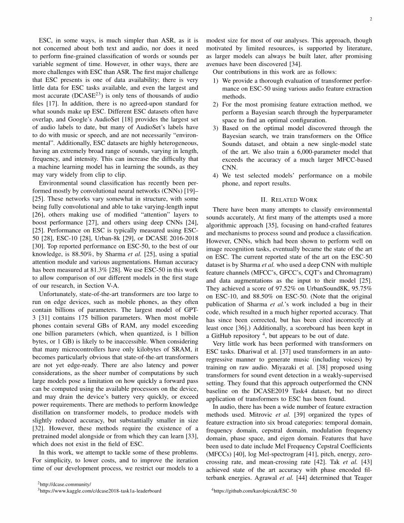
Fig. 1: We take six unique approaches to training a transformer on ESC. From left to right: raw amplitude reshaping, curvetokenization, MFCC feature extraction, multi-feature extraction, VQ-VAE tokenization, and Mel spectrograms. The transformerarchitecture is common between them, but the first layers vary. If a positional encoding is not shown for an architecture, thenno positional encoding is used.

Energy Operator-based Gammatone features outperform Melfilterbank energies. To combat noisy signals, Mogi and Kasai[45] proposed the use of Independent Component Analysisand Matching Pursuit, a method to extract features in the timedomain, rather than the frequency domain. With reference to[45], we note the assumption in our work that noise in anoffice environment will be minimal. Sharma et al. [25] obtainstate of the art using MFCC, GFCC, CQT, and Chromagramfeatures. Jukebox [11] was trained to differentiate music andartist styles using features extracted from three different VQ-VAEs, with varying vector lengths for each. A survey wasperformed in 2014 by Chachada and Kuo [46] that enumeratedthe features used in literature, with comparisons between each,but no more recent survey has been found. We choose some ofthe most successful of those feature extraction methods, andattempt some new ones designed specifically for transformers.

III. MODELS

Transformers are neural networks based on the self-attentionmechanism, which is an operation on sequences, relating posi-tions within the sequence in order to compute its representation[2]. We emphasize that the attention mechanism operates on alist of sequences, which means that the input to a transformermust be 2-dimensional (excluding batches). In NLP, we wantthe transformer to operate on sequences of words, characters,or something similar, which we refer to as “tokens”. Therefore,in order to meet the 2-dimensional input requirements of thetransformer, each token must be converted to a sequence. Thisis traditionally done using an embedding layer, which takes a

token, represented by the integer value of the token’s positionin a pre-computed vocabulary, and looks up its correspondingvector representation in a matrix. This embedding matrix isable to be learned. The embedding vector length is typicallyreferred to, in transformers, as the “hidden size”, or H . Thenumber of tokens is referred to by the length of the input L,also referred to as the sequence length. In this way, H definesthe number of dimensions that are used to represent tokens– where more dimensions typically mean greater learningcapacity – and L determines the context length, or windowsize, of the input.

Audio is represented at an extremely fine-grained level ofdetail (many samples per second), which poses challengesthat NLP does not have to face. For example, the commonsampling rate of 44.1 kHz in a 5-second audio clip (thelength of an audio clip in ESC-50) results in 220,500 samples.Combine this with the limitations of modern-day transformers,which, with some exceptions, are limited to roughly H < 2000tokens, depending on available hardware, and the task ofanalyzing audio data becomes quite difficult. There is hopethat this will change in the near future, with the creation oflinear-scaling models like BigBird [9] proven to have the samelearning capacity as BERT, and recent improvements in AIhardware by NVIDIA. But, for the sake of our discussion andanalysis, we will assume that we cannot use a transformersequence length of more than 2048.

This results in the maximum audio window that a trans-former can view – in the naıve case, where a single token isa single amplitude – to be 2048 samples, or 0.046 seconds

4

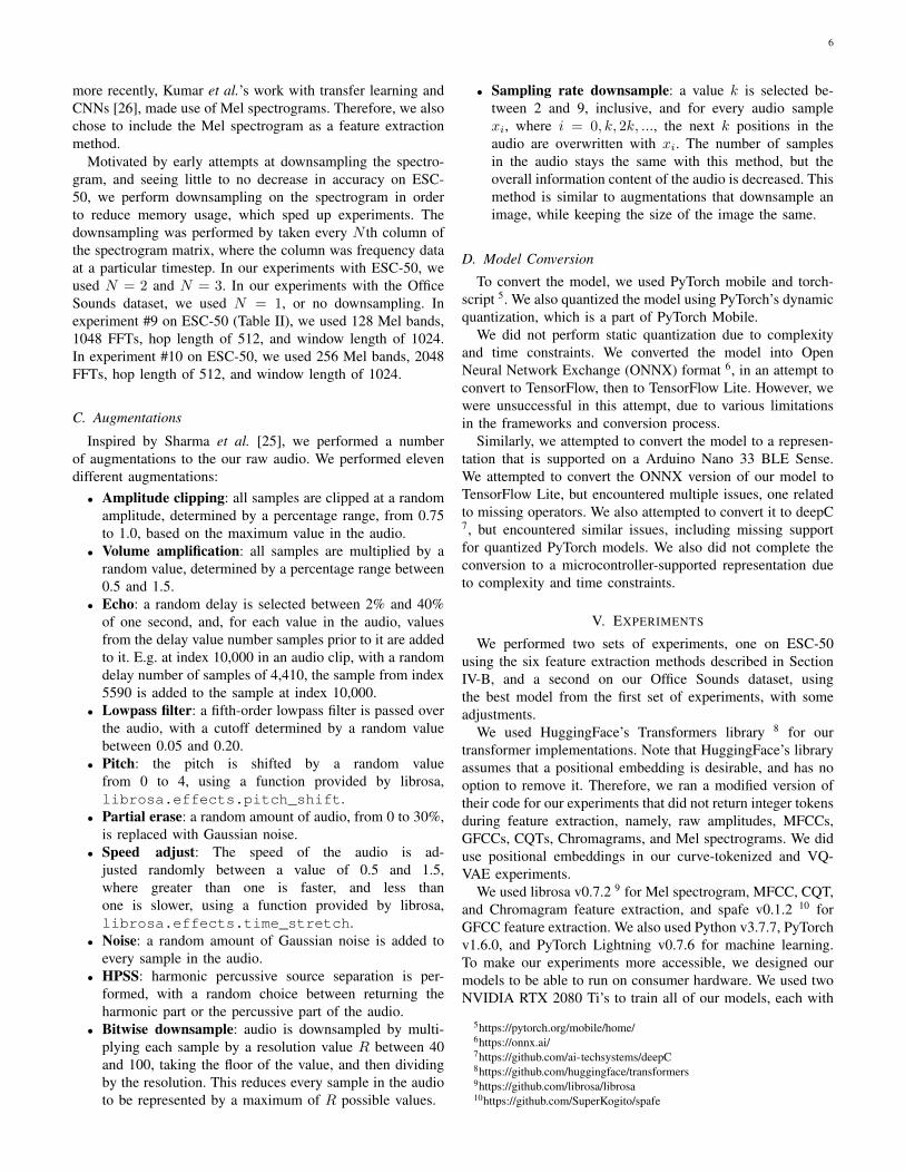
Fig. 2: The architecture on which our smallest Transformermodel is based. Visualization based on the diagram by Vaswaniet al. [2].

(46 milliseconds). Since sounds in the ESC-50 dataset oftenlast much longer than 46 milliseconds, we must thereforeabandon the naıve approach initially. The thought exists thatit is possible to downsample the audio to make the 2048sequence length be able to view a longer length of audio, butin practice this results in substantial information loss below16 kHz, and reduces model accuracy. We would like ourwork to be constrained solely by hardware and algorithmiclimitations, which have a strong likelihood of improving in thenear future, rather than constrained by the information contentin downsampled audio clips. Therefore, we assume a samplingrate above the Nyquist rate of 40 kHz for human-detectableaudio, and, specifically, use the conventional value of 44.1 kHzin all of our analyses.

All models in this work are based on BERT [3] or Al-BERT [47]. The Transformer base structure, whether BERTor AlBERT, does not change in this work. The only alterationperformed is to remove positional encodings for some models,which is noted in Figure 1 outside of the Transformer base.We note that our base structure in our ESC-50 experiments

does not make use of an embedding layer for input tokens, asis customary in language models, and any tokenizations andembeddings that do occur are explicitly called out in Figure1.

We make a change to the transformer design in our secondseries of experiments on the Office Sounds dataset (Figure 2),which allowed the size of the input to be decoupled from thesize of the model. In the six models shown in Figure 1, theinput must be either reshaped or the features must be extractedin the shape required to create a transformer of the desired size.For example, using 128 Mel bands when calculating MFCCsresulted in a transformer that had a maximum hidden sizeof 128. We remove this dependency in our Office Soundsexperiments by adding a mapping layer, as shown in Figure2. The mapping layer is simply a linear layer that takes inputof any size and maps it to the size of the transformer. Italso provides representational advantages, as this layer is ableto be learned, similar to the embedding layer in traditionaltransformers.

Additionally, in our ESC-50 experiments, we normalize allinputs to a number between 0 and 1 as a preprocessing step,where input is not tokenized. We remove this normalizationstep in our Office Sounds experiments, in favor of a batchnormalization layer [48], which may also have provided repre-sentational advantages to the Transformer by being learnable.

IV. APPROACH

We divide our approach below into sections on data, featureextraction, data augmentations, models, and model conversion.These methods work together to produce the results in SectionV.

A. Data

We use three datasets in this work, AudioSet [18], ESC-50 [28], and the Office Sounds dataset [49]. AudioSet isa large-scale weakly labeled dataset covering 527 differentsound types. The authors provide a balanced and unbalancedversion of the dataset; we use the balanced dataset, withsome additional balancing that we perform ourselves. Notethat in order to train on the audio from this dataset, we hadto download the audio from the sources used to compile thebalanced dataset. This was an error-prone process, as not allsources from the original AudioSet are still available. Moredetails on the datasets are available in Table I. ESC-50 is astrongly labeled dataset containing 50 different sound types.Each sound category contains 40 sounds, making it a balanceddataset. The Office Sounds dataset is both an unbalanced andweakly labeled dataset, owing to its origins in DCASE, butnearly the same number of audio files as ESC-50, with slightlylonger total length, and only 6 labels.

All audio files are converted to wave files, if they are notalready formatted as such. We read from each file at a samplingrate of 44100 Hz, in mono.

B. Feature Extraction

Feature extraction is a critical part of any machine learningarchitecture, and especially so for transformers. In fact, some

5

TABLE I: Information on the datasets used for training.

# of files # of hours # of audio typesAudioSet 37948 104.52 527ESC-50 2000 2.78 50Office Sounds 1608 2.80 6

of the critical work that went into making BERT such a successwas the use of word pieces, rather than words or characters[3]. In an attempt to discover a feature extraction method thatcan be of similar use in audio, we attempted several, someof which are well-known methods, others of which we haveadapted to our particular use case. The approaches can be seenin Figure 1.

1) Amplitude Reshaping: Motivated by works such asWaveNet [50], Jukebox [11] and, in general, the move towardmore “pure” data representations, we developed a method forthe transformer to work with raw amplitudes.

Using the notation in [51], we reshape audio in the fol-lowing way, where X is a sequence of amplitudes X ={x0, x1, ..., xn}, l is the sequence length, and d is the hiddendimension:

X ∈ Rl∗d×1 →reshape X ∈ Rl×d (1)

In this way, the amount of audio that we are able to processis a combination of the sequence length of the model, and thesize of the hidden dimension. Under this reshaping operation,with l = 512 and d = 512, we are able to process data up to262, 144 samples, or nearly 6 seconds.

2) Curve Tokenization: Curve tokenization is an audiotokenization method that we propose, based on WordPiecetokenization [52] in NLP. The intuition behind this methodis that, since audio signals typically vary smoothly, there mayexist a relatively small number of “curves” that can describeshort sequences of audio signals. These curves are commonlyrepresented in audio signals by sequences of floating pointnumbers. In wave files, a single audio amplitude can be one of65,536 values, or 216, values; as such, our audio is, effectively,already quantized. We term the quantization level of the audiothe resolution R.

Although wave file audio is already quantized, it is advanta-geous to quantize it further, as doing so reduces the maximumnumber of theoretical curves that can exist within any givensequence of audio. As an example, an 8-token curve withR = 100 has a maximum number of theoretical curves of1008. We performed quantizations at varying levels and foundthat R = 40 produces signals that remain highly recognizable.However, we chose R = 64 to ensure minimal informationloss.

Once quantized, we processed all the audio in our datasetusing a curve length of L samples. We created a dictionary,the key of which was every unique curve sequence that weencountered, and the value of which was the number of timesthat curve had been seen. At L = 8, sliding the the L-lengthwindow across each audio signal with a stride of 1, on ESC-50, this produced a dictionary of 3.87∗107 keys. We took thetop 50,000 sequences as our vocabulary, which covers 76.49%of the observed curves. At inference time, we used a stride of

L = 8, which resulted in a overall sequence length decrease ofL, also. We find that when curve-tokenizing our audio signalsin this way, 76.39% of the curves are found in the vocabulary,with the remaining 23.61% represented by the equivalent ofthe <UNK> token in NLP.

We also created a relative vocabulary by shifting the quan-tized values, such that the minimum value in any 8-tokenspan was set to zero, and all the other values maintained theirrelative position to the minimum, according to the Equation 2,where X = {x0, x1, ..., xn} is a span of audio with individualquantized values xi.

X =

n∑i=0

xi −min(X) (2)

Using the top 50,000 spans from the relative vocabulary, wefind that the it covers 85.44% of the number of unique spansin the dataset. When using the relative vocabulary to tokenizeaudio from the dataset, we find that an average 85.43% ofthe curves in each audio clip are represented, with 14.57%represented by the <UNK> token.

3) VQ-VAE: This method was motivated by Jukebox [11],which made use of vector-quantized variational autoencodersto produce compressed “codes” to represent audio. The VQ-VAEs that we trained used the code that the authors provided,and details on the specifics of training can be found in theirpaper. We used their default VQ-VAE hyperparameters, whichtrained three VQ-VAEs, each with a codebook size of 2048,a total model size of 1 billion parameters, and downsamplingrates of 128, 32, and 8. We trained the VQ-VAEs on AudioSetfor 500,000 steps. In our experiments, we use the VQ-VAEwith a downsampling rate of 32x.

4) MFCC: Mel-frequency cepstral coefficients (MFCCs)have a long history of use in audio classification problems [1],[25], [46], and so we tested their usefulness with transformers,as well. Unless otherwise mentioned, we used 128 mels, a hoplength of 512, a window length of 1024, and number of FFTsof 1024.

5) MFCC, GFCC, CQT, and Chromagram: Sharma et al.[25] reported a new state of the art on ESC-50, using fourfeature channels at once. They made use of MFCCs, gam-matone frequency cepstral coefficients (GFCCs), a constantQ-transform (CQT), and a chromagram. Roughly speaking,the usefulness of each feature can be broken down in thefollowing way: MFCCs are responsible for higher-frequencyaudio, such as speech or laughs; GFCCs are responsiblefor lower-frequency audio, such as footsteps or drums; CQTis responsible for music; and chromagrams are responsiblefor differentiating in difficult cases through the use of pitchprofiles. A more extended discussion of these features isavailable in Sharma et al.’s work [25]. We made use of thesame features with our transformer models, using the sameparameters for feature extraction as Sharma et al.. In order tofacilitate feeding the features into the transformer model, weconcatenate the features, creating a combined feature vectorof 512, which became the size of the hidden dimension.

6) Mel spectrogram: Other works obtaining high accuracieson ESC-50, such as the work by Salamon and Bello [20], and,

6

more recently, Kumar et al.’s work with transfer learning andCNNs [26], made use of Mel spectrograms. Therefore, we alsochose to include the Mel spectrogram as a feature extractionmethod.

Motivated by early attempts at downsampling the spectro-gram, and seeing little to no decrease in accuracy on ESC-50, we perform downsampling on the spectrogram in orderto reduce memory usage, which sped up experiments. Thedownsampling was performed by taken every N th column ofthe spectrogram matrix, where the column was frequency dataat a particular timestep. In our experiments with ESC-50, weused N = 2 and N = 3. In our experiments with the OfficeSounds dataset, we used N = 1, or no downsampling. Inexperiment #9 on ESC-50 (Table II), we used 128 Mel bands,1048 FFTs, hop length of 512, and window length of 1024.In experiment #10 on ESC-50, we used 256 Mel bands, 2048FFTs, hop length of 512, and window length of 1024.

C. Augmentations

Inspired by Sharma et al. [25], we performed a numberof augmentations to the our raw audio. We performed elevendifferent augmentations:

• Amplitude clipping: all samples are clipped at a randomamplitude, determined by a percentage range, from 0.75to 1.0, based on the maximum value in the audio.

• Volume amplification: all samples are multiplied by arandom value, determined by a percentage range between0.5 and 1.5.

• Echo: a random delay is selected between 2% and 40%of one second, and, for each value in the audio, valuesfrom the delay value number samples prior to it are addedto it. E.g. at index 10,000 in an audio clip, with a randomdelay number of samples of 4,410, the sample from index5590 is added to the sample at index 10,000.

• Lowpass filter: a fifth-order lowpass filter is passed overthe audio, with a cutoff determined by a random valuebetween 0.05 and 0.20.

• Pitch: the pitch is shifted by a random valuefrom 0 to 4, using a function provided by librosa,librosa.effects.pitch_shift.

• Partial erase: a random amount of audio, from 0 to 30%,is replaced with Gaussian noise.

• Speed adjust: The speed of the audio is ad-justed randomly between a value of 0.5 and 1.5,where greater than one is faster, and less thanone is slower, using a function provided by librosa,librosa.effects.time_stretch.

• Noise: a random amount of Gaussian noise is added toevery sample in the audio.

• HPSS: harmonic percussive source separation is per-formed, with a random choice between returning theharmonic part or the percussive part of the audio.

• Bitwise downsample: audio is downsampled by multi-plying each sample by a resolution value R between 40and 100, taking the floor of the value, and then dividingby the resolution. This reduces every sample in the audioto be represented by a maximum of R possible values.

• Sampling rate downsample: a value k is selected be-tween 2 and 9, inclusive, and for every audio samplexi, where i = 0, k, 2k, ..., the next k positions in theaudio are overwritten with xi. The number of samplesin the audio stays the same with this method, but theoverall information content of the audio is decreased. Thismethod is similar to augmentations that downsample animage, while keeping the size of the image the same.

D. Model Conversion

To convert the model, we used PyTorch mobile and torch-script 5. We also quantized the model using PyTorch’s dynamicquantization, which is a part of PyTorch Mobile.

We did not perform static quantization due to complexityand time constraints. We converted the model into OpenNeural Network Exchange (ONNX) format 6, in an attempt toconvert to TensorFlow, then to TensorFlow Lite. However, wewere unsuccessful in this attempt, due to various limitationsin the frameworks and conversion process.

Similarly, we attempted to convert the model to a represen-tation that is supported on a Arduino Nano 33 BLE Sense.We attempted to convert the ONNX version of our model toTensorFlow Lite, but encountered multiple issues, one relatedto missing operators. We also attempted to convert it to deepC7, but encountered similar issues, including missing supportfor quantized PyTorch models. We also did not complete theconversion to a microcontroller-supported representation dueto complexity and time constraints.

V. EXPERIMENTS

We performed two sets of experiments, one on ESC-50using the six feature extraction methods described in SectionIV-B, and a second on our Office Sounds dataset, usingthe best model from the first set of experiments, with someadjustments.

We used HuggingFace’s Transformers library 8 for ourtransformer implementations. Note that HuggingFace’s libraryassumes that a positional embedding is desirable, and has nooption to remove it. Therefore, we ran a modified version oftheir code for our experiments that did not return integer tokensduring feature extraction, namely, raw amplitudes, MFCCs,GFCCs, CQTs, Chromagrams, and Mel spectrograms. We diduse positional embeddings in our curve-tokenized and VQ-VAE experiments.

We used librosa v0.7.2 9 for Mel spectrogram, MFCC, CQT,and Chromagram feature extraction, and spafe v0.1.2 10 forGFCC feature extraction. We also used Python v3.7.7, PyTorchv1.6.0, and PyTorch Lightning v0.7.6 for machine learning.To make our experiments more accessible, we designed ourmodels to be able to run on consumer hardware. We used twoNVIDIA RTX 2080 Ti’s to train all of our models, each with

5https://pytorch.org/mobile/home/6https://onnx.ai/7https://github.com/ai-techsystems/deepC8https://github.com/huggingface/transformers9https://github.com/librosa/librosa10https://github.com/SuperKogito/spafe

7

TABLE II: Accuracy on ESC-50 dataset, running under various feature extraction and training schemes.

# Input Accuracy Samples Layers Heads Sequence Len Batch Augment Type

1 Amplitude reshaping 48.96 44100 8 8 256 16 True BERT2 Amplitude reshaping (Pretrained) 52.08 44100 16 16 256 16 True BERT3 VQ-VAE (32x) 31.77 16384 8 8 512 32 False BERT4 VQ-VAE (32x) 34.50 65536 8 8 2048 4 False BERT5 MFCC 53.13 44100 8 8 173 32 False BERT6 MFCC 58.33 44100 8 8 173 32 True BERT7 MFCC, GFCC, CQT, and Chromagram 59.38 88200 8 8 173 32 False BERT8 MFCC, GFCC, CQT, and Chromagram 59.90 88200 8 8 173 32 True BERT9 Mel spectrogram (Downsampled 3x) 60.45 220500 8 8 143 64 False AlBERT

10 Mel spectrogram (Optimized) 67.71 220500 16 16 215 16 True AlBERT11 Curve Tokenization (Relative) 7.81 4096 8 8 512 16 False BERT12 Curve Tokenization (Relative) 8.85 4096 8 8 512 16 True BERT13 Curve Tokenization (Absolute) 19.79 4096 8 8 512 16 False BERT14 Curve Tokenization (Absolute) 13.54 4096 8 8 512 16 True BERT

11GB of RAM, with the exception of the VQ-VAE with asequence length of 2048, experiment #4, for which we used aNVIDIA Tesla V100 with 16GB of RAM.

We trained using a learning rate of 0.0001, a learning ratewarmup of 10000 steps, and the Adam optimizer. Our datapipeline is implemented such that, every epoch, a randomslice is taken from each audio file, optionally passed throughaugmentations, and then passed to the model. This has theadvantage of vastly simplifying the data processing imple-mentation, and increasing the number of ways in which amodel can view a particular sound (assuming that the numberof samples viewed by the model is less than the numberof samples in the audio file). It does, however, have thedisadvantage of reading from every audio file an equal numberof times, regardless of the length of the audio. This was nota substantial issue for us, as AudioSet, ESC-50, and OfficeSounds all contain roughly the same length audio files withinthemselves.

A. Experiments on ESC-50

Table II describes the results of the trainings that weperformed with each of our model types, and we discuss theresults below.

1) Amplitude Reshaping: Experiment #1 with amplitudereshaping tested how well a transformer could learn to predictunder a few unusual circumstances: (1) the inputs to themodels are not constant with respect to tokens, as is usually thecase with learned embeddings, (2) the model is not pretrained,and (3) the dataset is small. The performance of this model wasfar below comparable CNNs, but better than expected, giventhat transformers traditionally are pretrained with massiveamounts of data, and are known to perform poorly whentrained on small datasets alone. We observed that the modelbegan to overfit around 60 epochs.

We also performed a supervised pretraining on reshaped rawamplitudes in experiment #2. This pretraining comes in theform of training on audio from AudioSet, described in TableI, which has 527 labels. We trained on AudioSet for 75 epochs,with augmentations, to a maximum top-1 validation accuracyof 6.36%, after which it began to overfit. We then took thatpretrained model, and finetuned it on ESC-50, without freezingany layers, according to standard practice with transformers.

It is notable that this pretraining increased accuracy by 3%,compared to the non-pretrained model. When pretrained on amuch larger dataset than AudioSet, it may be the case, as in[13], that a model like this obtains far higher accuracy whenfinetuned.

2) VQ-VAE: We were surprised by the inneffectiveness ofVQ-VAE codes in producing good classifications. Judging byJukebox [37], it seemed reasonable to believe that the VQ-VAEwould encode a substantial amount of knowledge in the codes,which, if they are enough to produce a good reconstructionof the original audio, might also be enough to produce aclassification. We did not find this to be the case, however, asthey vastly underperformed compared to MFCCs, raw audio,and others. We can think of several reasons for this: first, thelack of large-scale data reduces the maximum accuracy thatcan be obtained from any input by a transformer, and thismay be particularly true for VQ-VAE codes, since it couldhave been compounded by the lack of data supplied to boththe VQ-VAE in learning codes through AudioSet, and thelack of data in learning classifications in ESC-50. Second, theheterogeneity of sounds in AudioSet may have significantlylimited the VQ-VAE’s ability to represent sounds in the codes.It has previously been shown that VAEs in general do notperform well on heterogeneous datasets [53]. As such, ourVQ-VAE may not be able to perform as well on environmentsound tasks as it did on music tasks, given the large varietyof sounds present in ESC versus music.

Hypothesizing that the short sequence length of our firstexperiment (512) may have resulted in the transformer notbe able to have a sufficient view of the code to perform aclassification, we attempted a much longer sequence length,using a V100 GPU with 16GB of RAM. Even with a sequencelength of 2048, which translates to an effective number ofsamples of 65,536, or about 1.5 seconds, we did not observea substantial increase in accuracy, still falling far below otherfeature extraction methods.

As with the rest of the methods in this work, the first step toincreasing accuracy on ESC using VQ-VAE codes is to obtainmore data. Training on a much larger corpus of unlabeledaudio is entirely possible in the first step to creating VQ-VAE codes, and may improve the quality of the codes created.Additionally, using techniques such as the ones presented by

8

(a) (b)

(c) (d)

(e) (f)

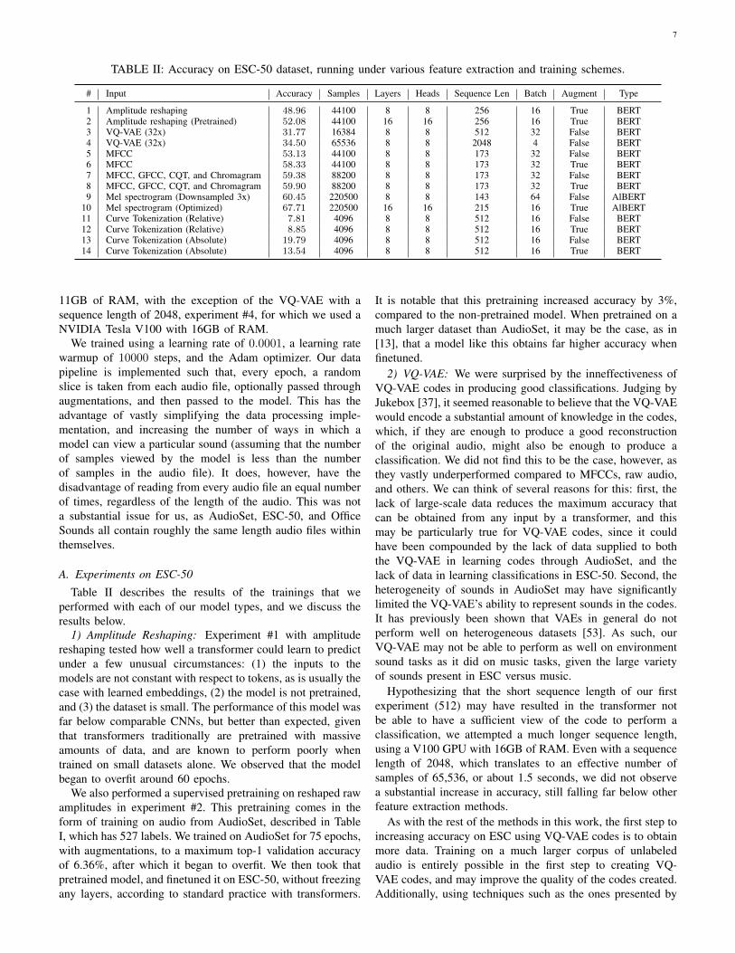
Fig. 3: Validation accuracy on AlBERT, trained using a Mel spectrogram with varying parameters, aggregated over a total of159 runs. The figures show results as the following parameters are varied: (a) augmentations, (b) number of samples viewedby the model at once, (c) number of Mel bands in the Mel spectrogram, (d) number of hidden layers in the model, or thedepth of the model, (e) number of attention heads, and (f) the hop length when calculating the Mel spectrogram.

Nazabal et al. [53], to alter the VQ-VAE to enable to it betterhandle heterogeneous data, may help as well. It may also beof value to perform a pretraining step, either supervised orunsupervised, and finetune on more ESC data. However, evenwith all such adjustments, it seems unlikely that VQ-VAEcodes will exceed MFCCs, Mel spectrograms or raw audioin predictive capability.

3) MFCC, GFCC, CQT, and Chromagram: In experiments#5 and #6, we observe that augmentations make a substantial(5.2%) impact on accuracy. We also see that MFCC’s performbetter, though only slightly so, than raw amplitudes. Theseexperiments were performed with 128 Mel bands, whichresulted in the hidden size H of the model to be 128 as well.These models began to overfit around 50 epochs.

Experiments #7 and #8 showed that adding additionalfeature extraction methods improved the accuracy of the modelbeyond only using MFCCs, especially in the non-augmentedcase. However, when augmented, the model did not show any

major improvements, as had occurred with MFCCs. This isdifferent than the results by Sharma et al. [25], which hadused augmentations to improve accuracy by more than 3%.However, we note that for our purposes – inferring at theedge – the cost of computing features using all four extractionmethods becomes prohibitive, and the model would have beenunlikely to be of use at the edge, even it it had obtainedhigh accuracy. We also found that extracting these featuresat training time resulted in extremely slow training, whichhindered additional experimentation with these features.

4) Mel Spectrogram and Hyperparameter Search: Wetrained using a Mel spectrogram in experiments #9 and #10,and obtained accuracy that outperformed any other featureextraction methods. This is particularly advantageous at theedge, since computing a Mel spectrogram is a reasonablyinexpensive operation. Of note, as well, is the fact that thiswas obtained with a smaller sequence length than experiments#7 and #8, due to the 3x downsampling that we performed.

9

TABLE III: Transformer accuracy on Office Sounds dataset for various models, ordered by number of paramaters. All modelswere based on BERT, and had the feed-forward layer size set to 4H .

# Input Accuracy Params Multiply-Adds Samples Layers Hidden Heads Sequence Len Batch Augment

1 Mel spectrogram 81.48% 5,954 5,638 44100 1 16 2 86 64 True2 Mel spectrogram 93.21% 6,642 5,982 220500 1 16 2 430 64 True3 Mel spectrogram 95.31% 213,858 210,414 220500 4 64 4 430 64 True4 Mel spectrogram 93.75% 25,553,762 25,506,734 220500 8 512 8 430 16 True5 Mel spectrogram 89.38% 25,553,762 25,506,734 220500 8 512 8 430 16 False

TABLE IV: CNN accuracy on Office Sounds dataset, ordered by accuracy.

# Input Accuracy Params Multiply-Adds Samples Batch Augment

1 MFCC 92.97% 4,468,022 478,869,984 110250 64 True2 MFCC 92.19% 4,468,022 478,869,984 110250 64 False3 MFCC 91.41% 4,468,022 956,052,832 220500 16 False

We also used AlBERT, and a longer sequence length thatother models, which may have contributed to the improvedperformance. Judging by the performance of BERT-basedtransformers trained on Office Sounds, however, it seems un-likely that AlBERT would result in a significant performanceimprovement alone. The impact of number of samples isdiscussed below.

Since this was our best-performing model, we performed ahyperparameter search to determine the optimal parameters.All training was performed using AlBERT as the base model,with a downsampling rate of 2x. We performed 159 trainingruns, which are aggregated into the graphs in Figure 3.

Some clear improvements result by changing certain pa-rameters. The most obvious is the number of samples that arepassed into the Mel spectrogram, which, as it increases, alsoincreases the maximum possible validation accuracy. We chosea peak of 220,500 samples, or 5 seconds of audio, becausefiles in ESC-50 audio have a maximum length of 5 seconds.As can be seen, a model’s access to the full file’s worth ofdata improves its ability to classify well.

Another clear result is the importance of using more than80 Mel bands when creating the Mel spectrogram. This resultis particularly important, as many research works make use of80 Mels or less [15], [38], [41], [42], [54], [55], which likelyreduced accuracy in those works.

5) Curve Tokenization: As a first attempt in literature attokenizing audio based on curves, for the purpose of traininga transformer, we find that they provide very little predictivepower. There may be several reasons for this, the first of whichis the small number of samples over which the model can viewa sound. Since every 8 samples is quantized and convertedinto a token, using a sequence length of 512, the number ofeffective samples is 4096, which is only 93 milliseconds ofaudio. This is likely a limiting factor on the predictive abilityof the model, and a model able to handle a much longersequence length would likely perform better. It is also likelythat quantizing it reduced the information content of the audio,and further reduced the predictive power.

In the case of absolute curves, we find that augmentationssubstantially reduce accuracy. This is likely due to the fact thatour vocabulary was created on ESC-50 without augmentations,

so the curves that appear with augmentations result in manymore <UNK> tokens. We see a slight increase in relative curvetokenization with augmentations, but, given the incredibly lowaccuracy of the model, find it to be of little interest.

Overall, we consider it unlikely that curve tokenizationwould ever beat out more well-known feature extraction tech-niques. It removes too much information, such as vital fre-quency and phase information, which other feature extractionmethods allow the transformer to make use of. Nonetheless, weconsider it an interesting experiment in possible tokenizationtechniques for transformers on audio.

B. Experiments on Office SoundsAfter completing our experiments on ESC-50, we trained on

the Office Sounds dataset [49]. We used BERT-based modelsonly, with an emphasis on model size, specifically on reducingthe model size while maintaining accuracy in order to performmore efficient processing at the edge. We were particularlyinterested in models which were capable of being run onmicrocontrollers; in our case, we chose a target model sizeof 256KB or less – the available SRAM on the ArduinoNano 33 BLE Sense – which meant that the model must beless than 250,000 parameters when quantized. There are, ofcourse, methods to run larger models with less SRAM, suchas MCUNet [56], but we left such optimizations to a futurework, focusing on the generic case of running a transformeron a microcontroller without any special optimizations.

We made several adjustments between our ESC-50 experi-ments and our Office Sounds experiments, described in SectionIII, which enabled us to experiment with vastly different modelsizes. We began by choosing a model with parameters simi-lar to our best-performing models from the hyperparametersearch. We chose the model seen in experiments #4 and #5 ofTable III, based on Mel spectrogram input with a hop lengthof 512, window size of 1024, number of FFTs of 1024, andMel bands of 128. It had 8 layers, and a hidden size H largerthan we had been able to use in the ESC-50 experiments, of512, and 8 heads. We also removed downsampling, makingthe sequence length much longer than before, but still ableto fit within the constraints of consumer-grade GPUs whilemaintaining a reasonable batch size. These models obtained a

10

maximum validation accuracy of 93.75%, with augmentations,and began to overfit after 200-300 epochs.

In order to facilitate accurate comparisons to our previouswork [49], we reimplemented and performed training on OfficeSounds using MFCCs as input to a CNN, shown in Table IV.Following that work, the CNN was an exact reimplementationof Kumar et al.’s model in [26]. We trained the model, non-augmented, on ESC-50 to confirm accurate implementation,and obtained 81.25%, which is very close to the 83.5% modelaccuracy that Kumar et al. reported for their model that hadbeen pretrained on AudioSet. We performed training of thisMFCC-based CNN against Office Sounds, using a randomslice of the each audio file in each epoch, and obtained amaximum of 92.97% accuracy, using augmentations on 2.5seconds of audio. This corresponds to the results obtained in[49], even though the training scheme is slightly different.The model contained 4.5 million parameters, and nearly 500million multiply-adds. The inference time of this model on aSamsung Galaxy S9 was an average of 57 milliseconds [49],non-augmented and non-quantized, using TensorFlow Lite,shown in Table V. We note that augmentations had a smallpositive effect on validation accuracy, and that increasing thevisible audio window size from 2.5 to 5 seconds had a slightlynegative effect.

In comparing the Office Sounds transformers to the OfficeSounds CNNs, we find that the transformers outperform theCNN, while being much smaller. A model with 95.2% lessparameters, transformer experiment #3, outperformed the CNNby more than 2%. The smallest model that we trained on5 seconds of audio, experiment #2, 99.85% smaller thanthe CNN, also outperformed the CNNs. This is unexpected,since CNNs far outperformed transformers on the ESC-50experiments. Our hypothesis is that the increased number ofexample data for each class in Office Sounds (200 or moreper class, compared to 40 per class in ESC-50), assisted inpreventing as rapid overfitting as was observed in ESC-50.This can be tested by reducing the number of samples in OfficeSounds and running these experiments again; we leave this fora future work.

We also trained our smallest model on one second of data(experiment #1), and found that it substantially reduced theaccuracy of the model. Interestingly, for some applications,it may be worthwhile to process only one second of audiowith reduced accuracy, as it reduces the cost of featureextraction and allows the model to be run more frequently.Also, predictions over each second can be aggregated acrossa longer time span via majority voting, or something similar,in order to potentially produce more accurate predictions.

C. Inference at the Edge

Table V shows feature extraction and inference times on aSamsung Galaxy S9. This model uses a transformer based ona Mel spectrogram, processing 5 seconds of audio data andproducing a classification using ESC-50 labels. We observethat, even on a device more than two years old, inference isstill fast enough to be performed many times a second. Wealso find that quantization results in lowered latency (about

21% with dynamic quantization), which further increases thepotential model size. Static quantization is likely to reducelatency further, as dynamic quantization does not quantizemodel activations.

TABLE V: Inference times of selected models on an edgedevice. Models are run on a Samsung Galaxy S9 usingPyTorch Mobile, except for the first, which was run with Ten-sorFlow Lite. Results are averaged over 10 runs. Quantizationis PyTorch dynamic quantization.

Experiment Params Mult-Adds Latency (ms)

MFCC CNN from [49] 4,468,022 478,869,984 57ESC-50 #10 958,146 948,888 111ESC-50 #10, Quant. 958,146 948,888 88Office Sounds, Trans. #2 6,642 5,982 7

We also observed a substantially decreased inference timefrom our smallest model, as expected, inferring 93% fasterthan the 1-million parameter transformer. It was surprising tofind that the much larger CNN had faster inference times thanthe 1-million parameter transformer, however, this may be dueto optimizations in TensorFlow Lite that are not present inPyTorch Mobile, or simply that CNN operations are optimizedfurther than transformer operations on edge devices.

VI. CONCLUSION AND FUTURE WORK

Efficient edge processing is a challenging, but critical taskwhich will become increasingly important in the future. Toaide in this task, we trained a 6,000-parameter transformeron the Office Sounds dataset that outperforms a CNN morethan 700x larger than it. This enables accurate and efficientenvironmental sound classification of office sounds on edgedevices, even on inexpensive microcontrollers, resulting ininference times on a Samsung Galaxy S9 that are 88% fasterthan a CNN with comparable accuracy. We find that modelstrained in traditional frameworks (like PyTorch) have relativelylittle support for conversion to models that can be run at theedge (like on a microcontroller), even with the developmentof ONNX.

Our ESC-50 transformer models did not outperform CNNs,as they did on Office Sounds. Understanding this, and findingsolutions to the problem of training transformers on smallaudio datasets, is a crucial future work. Solutions may comethrough large amounts of unsupervised pretraining, throughan architectural change, or though improved supervised ESCdatasets. In any case, our work provides groundwork uponwhich these questions can be answered.

The small size and efficiency of the transformer we trainedraises questions about the cost of retraining. It may be that,because there are so few operations (<6,000) required ina forward pass, that on-device retraining becomes possible,similar to what is done on Coral Edge TPUs through theimprinting engine [57]. This would have vast implications onthe future of intelligent edge analytics, and even a variety ofuser applications.

11

REFERENCES

[1] M. Cowling and R. Sitte, “Comparison of techniques for environmentalsound recognition,” Pattern recognition letters, vol. 24, no. 15, pp. 2895–2907, 2003.

[2] A. Vaswani, N. Shazeer, N. Parmar, J. Uszkoreit, L. Jones, A. N. Gomez,Ł. Kaiser, and I. Polosukhin, “Attention is all you need,” in Advancesin neural information processing systems, 2017, pp. 5998–6008.

[3] J. Devlin, M.-W. Chang, K. Lee, and K. Toutanova, “Bert: Pre-trainingof deep bidirectional transformers for language understanding,” arXivpreprint arXiv:1810.04805, 2018.

[4] Z. Yang, Z. Dai, Y. Yang, J. Carbonell, R. R. Salakhutdinov, andQ. V. Le, “Xlnet: Generalized autoregressive pretraining for languageunderstanding,” in Advances in neural information processing systems,2019, pp. 5753–5763.

[5] C. Raffel, N. Shazeer, A. Roberts, K. Lee, S. Narang, M. Matena,Y. Zhou, W. Li, and P. J. Liu, “Exploring the limits of trans-fer learning with a unified text-to-text transformer,” arXiv preprintarXiv:1910.10683, 2019.

[6] A. Radford, K. Narasimhan, T. Salimans, and I. Sutskever, “Improvinglanguage understanding by generative pre-training,” 2018.

[7] A. Radford, J. Wu, R. Child, D. Luan, D. Amodei, and I. Sutskever,“Language models are unsupervised multitask learners,” OpenAI Blog,vol. 1, no. 8, p. 9, 2019.

[8] T. B. Brown, B. Mann, N. Ryder, M. Subbiah, J. Kaplan, P. Dhariwal,A. Neelakantan, P. Shyam, G. Sastry, A. Askell et al., “Language modelsare few-shot learners,” arXiv preprint arXiv:2005.14165, 2020.

[9] M. Zaheer, G. Guruganesh, A. Dubey, J. Ainslie, C. Alberti, S. Ontanon,P. Pham, A. Ravula, Q. Wang, L. Yang et al., “Big bird: Transformersfor longer sequences,” arXiv preprint arXiv:2007.14062, 2020.

[10] M. Chen, A. Radford, R. Child, J. Wu, H. Jun, P. Dhariwal, D. Luan,and I. Sutskever, “Generative pretraining from pixels,” in Proceedingsof the 37th International Conference on Machine Learning, 2020.

[11] P. Dhariwal, H. Jun, C. Payne, J. W. Kim, A. Radford, andI. Sutskever, “Jukebox: A generative model for music,” arXiv preprintarXiv:2005.00341, 2020.

[12] A. Van Den Oord, O. Vinyals et al., “Neural discrete representationlearning,” in Advances in Neural Information Processing Systems, 2017,pp. 6306–6315.

[13] Anonymous, “An image is worth 16x16 words: Transformers forimage recognition at scale,” in Submitted to International Conferenceon Learning Representations, 2021, under review. [Online]. Available:https://openreview.net/forum?id=YicbFdNTTy

[14] N.-Q. Pham, T.-S. Nguyen, J. Niehues, M. Muller, S. Stuker, andA. Waibel, “Very deep self-attention networks for end-to-end speechrecognition.” [Online]. Available: http://arxiv.org/abs/1904.13377

[15] R. Zhang, H. Wu, W. Li, D. Jiang, W. Zou, and X. Li, “Transformerbased unsupervised pre-training for acoustic representation learning,”arXiv:2007.14602 [cs, eess], Jul. 2020, arXiv: 2007.14602. [Online].Available: http://arxiv.org/abs/2007.14602

[16] Y. Shi, Y. Wang, C. Wu, C. Fuegen, F. Zhang, D. Le, C.-F. Yeh, andM. L. Seltzer, “Weak-Attention Suppression For Transformer BasedSpeech Recognition,” arXiv:2005.09137 [cs, eess], May 2020, arXiv:2005.09137. [Online]. Available: http://arxiv.org/abs/2005.09137

[17] D. Stowell, D. Giannoulis, E. Benetos, M. Lagrange, and M. D.Plumbley, “DCASE 2016 Acoustic Scene Classification UsingConvolutional Neural Networks,” IEEE Transactions on Multimedia,vol. 17, no. 10, pp. 1733–1746, Oct. 2015. [Online]. Available:http://ieeexplore.ieee.org/document/7100934/

[18] J. F. Gemmeke, D. P. Ellis, D. Freedman, A. Jansen, W. Lawrence, R. C.Moore, M. Plakal, and M. Ritter, “Audio set: An ontology and human-labeled dataset for audio events,” in 2017 IEEE International Conferenceon Acoustics, Speech and Signal Processing (ICASSP). IEEE, 2017,pp. 776–780.

[19] W. Dai, C. Dai, S. Qu, J. Li, and S. Das, “Very deep convolutional neuralnetworks for raw waveforms,” in 2017 IEEE International Conferenceon Acoustics, Speech and Signal Processing (ICASSP), pp. 421–425,ISSN: 2379-190X.

[20] J. Salamon and J. P. Bello, “Deep Convolutional Neural Networksand Data Augmentation for Environmental Sound Classification,” IEEESignal Processing Letters, vol. 24, no. 3, pp. 279–283, Mar. 2017.[Online]. Available: http://ieeexplore.ieee.org/document/7829341/

[21] Y. Tokozume and T. Harada, “Learning environmental sounds withend-to-end convolutional neural network,” in 2017 IEEE InternationalConference on Acoustics, Speech and Signal Processing (ICASSP), pp.2721–2725, ISSN: 2379-190X.

[22] X. Zhang, Y. Zou, and W. Shi, “Dilated convolution neural networkwith LeakyReLU for environmental sound classification,” in 2017 22ndInternational Conference on Digital Signal Processing (DSP), pp. 1–5,ISSN: 2165-3577.

[23] S. Abdoli, P. Cardinal, and A. Lameiras Koerich, “End-to-endenvironmental sound classification using a 1D convolutional neuralnetwork,” Expert Systems with Applications, vol. 136, pp. 252–263,Dec. 2019. [Online]. Available: https://linkinghub.elsevier.com/retrieve/pii/S0957417419304403

[24] A. Khamparia, D. Gupta, N. G. Nguyen, A. Khanna, B. Pandey, andP. Tiwari, “Sound classification using convolutional neural network andtensor deep stacking network,” vol. 7, pp. 7717–7727, conference Name:IEEE Access.

[25] J. Sharma, O.-C. Granmo, and M. Goodwin, “Environment SoundClassification using Multiple Feature Channels and Attention basedDeep Convolutional Neural Network,” arXiv:1908.11219 [cs, eess,stat], Apr. 2020, arXiv: 1908.11219. [Online]. Available: http://arxiv.org/abs/1908.11219

[26] A. Kumar, M. Khadkevich, and C. Fugen, “Knowledge Transferfrom Weakly Labeled Audio Using Convolutional Neural Network forSound Events and Scenes,” in 2018 IEEE International Conferenceon Acoustics, Speech and Signal Processing (ICASSP). Calgary,AB: IEEE, Apr. 2018, pp. 326–330. [Online]. Available: https://ieeexplore.ieee.org/document/8462200/

[27] Z. Zhang, S. Xu, S. Zhang, T. Qiao, and S. Cao, “LearningAttentive Representations for Environmental Sound Classification,”IEEE Access, vol. 7, pp. 130 327–130 339, 2019. [Online]. Available:https://ieeexplore.ieee.org/document/8823934/

[28] K. J. Piczak, “Esc: Dataset for environmental sound classification,” inProceedings of the 23rd ACM international conference on Multimedia.ACM, 2015, pp. 1015–1018.

[29] J. Salamon, C. Jacoby, and J. P. Bello, “A dataset and taxonomy forurban sound research,” in Proceedings of the 22nd ACM internationalconference on Multimedia. ACM, 2014, pp. 1041–1044.

[30] D. Giannoulis, E. Benetos, D. Stowell, M. Rossignol, M. Lagrange, andM. D. Plumbley, “Detection and classification of acoustic scenes andevents: An ieee aasp challenge,” in 2013 IEEE Workshop on Applicationsof Signal Processing to Audio and Acoustics, Oct 2013, pp. 1–4.

[31] T. B. Brown, B. Mann, N. Ryder, M. Subbiah, J. Kaplan, P. Dhariwal,A. Neelakantan, P. Shyam, G. Sastry, A. Askell, S. Agarwal,A. Herbert-Voss, G. Krueger, T. Henighan, R. Child, A. Ramesh, D. M.Ziegler, J. Wu, C. Winter, C. Hesse, M. Chen, E. Sigler, M. Litwin,S. Gray, B. Chess, J. Clark, C. Berner, S. McCandlish, A. Radford,I. Sutskever, and D. Amodei, “Language Models are Few-ShotLearners,” arXiv:2005.14165 [cs], May 2020, arXiv: 2005.14165.[Online]. Available: http://arxiv.org/abs/2005.14165

[32] V. Sanh, L. Debut, J. Chaumond, and T. Wolf, “DistilBERT, adistilled version of BERT: smaller, faster, cheaper and lighter,”arXiv:1910.01108 [cs], Feb. 2020, arXiv: 1910.01108. [Online].Available: http://arxiv.org/abs/1910.01108

[33] S. Sun, Y. Cheng, Z. Gan, and J. Liu, “Patient knowledgedistillation for BERT model compression.” [Online]. Available:http://arxiv.org/abs/1908.09355

[34] I. Turc, M.-W. Chang, K. Lee, and K. Toutanova, “Well-read studentslearn better: On the importance of pre-training compact models,” arXivpreprint arXiv:1908.08962, 2019.

[35] C. Couvreur, V. Fontaine, P. Gaunard, and C. G. Mubikangiey, “Au-tomatic classification of environmental noise events by hidden markovmodels,” p. 20.

[36] Z. Mushtaq, S.-F. Su, and Q.-V. Tran, “Spectral images based environ-mental sound classification using cnn with meaningful data augmenta-tion,” Applied Acoustics, vol. 172, p. 107581.

[37] P. Dhariwal, H. Jun, C. Payne, J. W. Kim, A. Radford, andI. Sutskever, “Jukebox: A generative model for music.” [Online].Available: http://arxiv.org/abs/2005.00341

[38] K. Miyazaki, T. Komatsu, T. Hayashi, S. Watanabe, T. Toda, andK. Takeda, “Weakly-supervised sound event detection with self-attention,” in ICASSP 2020 - 2020 IEEE International Conference on

12

Acoustics, Speech and Signal Processing (ICASSP), pp. 66–70, ISSN:2379-190X.

[39] D. Mitrovic, M. Zeppelzauer, and C. Breiteneder, “Features for content-based audio retrieval,” in Advances in computers. Elsevier, 2010,vol. 78, pp. 71–150.

[40] V. Boddapati, A. Petef, J. Rasmusson, and L. Lundberg, “Classifyingenvironmental sounds using image recognition networks,” ProcediaComputer Science, vol. 112, pp. 2048–2056, 2017. [Online]. Available:https://linkinghub.elsevier.com/retrieve/pii/S1877050917316599

[41] K. J. Piczak, “Environmental sound classification with convolutionalneural networks,” in 2015 IEEE 25th International Workshop on Ma-chine Learning for Signal Processing (MLSP), pp. 1–6, ISSN: 2378-928X.

[42] J. Li, W. Dai, F. Metze, S. Qu, and S. Das, “A comparison of DeepLearning methods for environmental sound detection,” in 2017 IEEEInternational Conference on Acoustics, Speech and Signal Processing(ICASSP). New Orleans, LA: IEEE, Mar. 2017, pp. 126–130. [Online].Available: http://ieeexplore.ieee.org/document/7952131/

[43] R. N. Tak, D. M. Agrawal, and H. A. Patil, “Novel Phase Encoded MelFilterbank Energies for Environmental Sound Classification,” in PatternRecognition and Machine Intelligence, B. U. Shankar, K. Ghosh, D. P.Mandal, S. S. Ray, D. Zhang, and S. K. Pal, Eds. Cham: SpringerInternational Publishing, 2017, vol. 10597, pp. 317–325. [Online].Available: http://link.springer.com/10.1007/978-3-319-69900-4 40

[44] D. M. Agrawal, H. B. Sailor, M. H. Soni, and H. A. Patil, “Novel TEO-based Gammatone features for environmental sound classification,”in 2017 25th European Signal Processing Conference (EUSIPCO).Kos, Greece: IEEE, Aug. 2017, pp. 1809–1813. [Online]. Available:http://ieeexplore.ieee.org/document/8081521/

[45] R. Mogi and H. Kasai, “Noise-Robust environmental sound classificationmethod based on combination of ICA and MP features,” ArtificialIntelligence Research, vol. 2, no. 1, p. p107, Nov. 2012. [Online].Available: http://www.sciedu.ca/journal/index.php/air/article/view/1399

[46] S. Chachada and C.-C. J. Kuo, “Environmental sound recognition: asurvey,” APSIPA Transactions on Signal and Information Processing,vol. 3, p. e14, 2014. [Online]. Available: https://www.cambridge.org/core/product/identifier/S2048770314000122/type/journal article

[47] Z. Lan, M. Chen, S. Goodman, K. Gimpel, P. Sharma, and R. Soricut,“ALBERT: A Lite BERT for Self-supervised Learning of LanguageRepresentations,” arXiv:1909.11942 [cs], Feb. 2020, arXiv: 1909.11942.[Online]. Available: http://arxiv.org/abs/1909.11942

[48] S. Ioffe and C. Szegedy, “Batch normalization: Accelerating deepnetwork training by reducing internal covariate shift,” arXiv preprintarXiv:1502.03167, 2015.

[49] D. Elliott, E. Martino, C. E. Otero, A. Smith, A. M. Peter, B. Luchter-hand, E. Lam, and S. Leung, “Cyber-physical analytics: Environmentalsound classification at the edge,” in 2020 IEEE 6th World Forum onInternet of Things (WF-IoT). IEEE, 2020, pp. 1–6.

[50] A. v. d. Oord, S. Dieleman, H. Zen, K. Simonyan, O. Vinyals, A. Graves,N. Kalchbrenner, A. Senior, and K. Kavukcuoglu, “Wavenet: A gener-ative model for raw audio,” arXiv preprint arXiv:1609.03499, 2016.

[51] M. Sperber, J. Niehues, G. Neubig, S. Stuker, and A. Waibel,“Self-Attentional Acoustic Models,” arXiv:1803.09519 [cs], Jun. 2018,arXiv: 1803.09519. [Online]. Available: http://arxiv.org/abs/1803.09519

[52] Y. Wu, M. Schuster, Z. Chen, Q. V. Le, M. Norouzi, W. Macherey,M. Krikun, Y. Cao, Q. Gao, K. Macherey et al., “Google’s neuralmachine translation system: Bridging the gap between human andmachine translation,” arXiv preprint arXiv:1609.08144, 2016.

[53] A. Nazabal, P. M. Olmos, Z. Ghahramani, and I. Valera, “Handlingincomplete heterogeneous data using vaes,” Pattern Recognition, p.107501, 2020.

[54] Y. Zhao, X. Wu, Y. Ye, J. Guo, and K. Zhang, “Musicoder: A uni-versal music-acoustic encoder based on transformers,” arXiv preprintarXiv:2008.00781, 2020.

[55] Y. Jiao, “Translate reverberated speech to anechoic ones: Speech dere-verberation with bert,” arXiv preprint arXiv:2007.08052, 2020.

[56] J. Lin, W.-M. Chen, Y. Lin, J. Cohn, C. Gan, and S. Han, “Mcunet: Tinydeep learning on iot devices,” arXiv preprint arXiv:2007.10319, 2020.

[57] “Retrain a classification model on-device with weightimprinting.” [Online]. Available: https://coral.ai/docs/edgetpu/retrain-classification-ondevice/

David Elliott (M’2017) is a Ph.D. candidate inComputer Engineering at Florida Institute of Tech-nology. He completed his B.S. in Computer Engi-neering in 2017, and his M.S. in the same in 2018.He has three years of industry experience, wherehe has made contributions in the areas of cloudsystems, cyber resiliency, machine learning, and theInternet of Things. His work has been presented tohigh-level government executives, and used to defineand advance the state of the art in practice. He hasauthored several papers, appearing in IEEE CLOUD

and IEEE World Forum on the Internet of Things.

Carlos E. Otero (SM’09) received a B.S. degreein computer science, a M.S. degree in softwareengineering, a M.S. degree in systems engineering,and a Ph.D. degree in computer engineering fromFlorida Institute of Technology, Melbourne. He iscurrently Associate Professor and the Co-Directorof the Center for Advanced Data Analytics andSystems (CADAS), Florida Institute of Technology.He was an Assistant Professor with the University ofSouth Florida and the University of Virginia at Wise.He has authored over 70 papers in wireless sensor

networks, Internet-of-Things, big data, and hardware/software systems. Hisresearch interests include performance analysis, evaluation, and optimizationof computer systems, including wireless ad hoc and sensor networks. He hasover twelve years of industry experience in satellite communications systems,command and control systems, wireless security systems, and unmanned aerialvehicle systems.

Steven Wyatt (M’2020) performs research and de-velopment at Northrop Grumman Corporation whilecompleting his B.S. in Computer Engineering atFlorida Institute of Technology. He has extensive ex-perience in fuzzing, wireless systems, and machinelearning. His work has been the basis for corporateAI strategy, and he continues to improve the stateof the art in efficient edge analytics through hisresearch.

Evan Martino (M’2020) completed his B.S in Com-puter Engineering, and is pursuing his M.S in Com-puter Engineering at the Florida Institute of Tech-nology. He has two years of industry experience,performing research and development in networking,distributed systems, and machine learning. He hasbeen published in the World Forum on the Internetof things, and his work is used to provide state-of-the-art analytics in production systems today.