tion curve precision in routine analysis

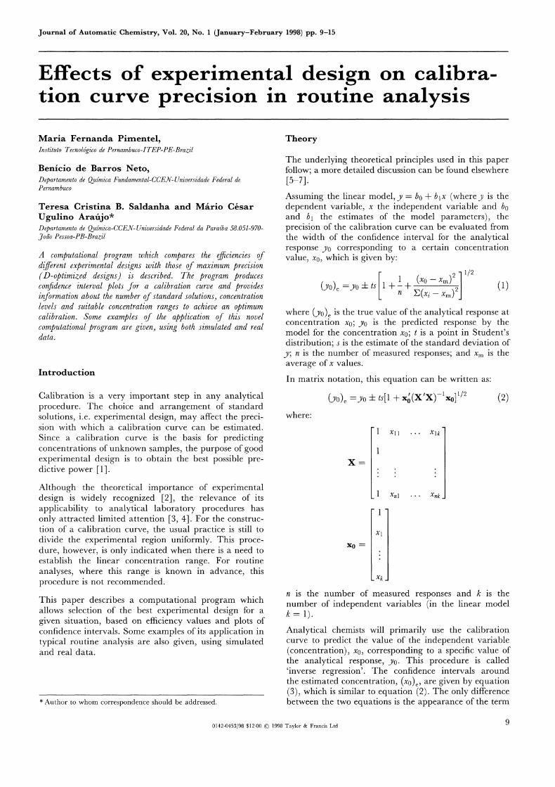
Journal of Automatic Chemistry, Vol. 20, No. (January-February 1998) pp. 9-15

Effects oftion curve

experimental design on calibra-precision in routine analysis

Maria Fernanda Pimentel,Instituto Tecnoldgico de Pernambuco-ITEP-PE-Brazil

Benicio de Barros Neto,Departamento de Qu{mica Fundamental-CCEN-Universidade Federal dePernambuco

Teresa Cristina B. Saldanha and MArio C6sarUgulino Arafijo*Departamento de Qu{mica-CCEN-Universidade Federal da Paraiba 58.051-970-Jodo Pessoa-PB-Brazil

A computational program which compares the effciencies ofdifferent experimental designs with those of maximum precision(D-optimized designs) is described. The program producesconfidence interval plots for a calibration curve and providesinformation about the number of standard solutions, concentrationlevels and suitable concentration ranges to achieve an optimumcalibration. Some examples of the application of this novelcomputational program are given, using both simulated and realdata.

Introduction

Calibration is a very important step in any analyticalprocedure. The choice and arrangement of standardsolutions, i.e. experimental design, may affect the preci-sion with which a calibration curve can be estimated.Since a calibration curve is the basis for predictingconcentrations of unknown samples, the purpose of goodexperimental design is to obtain the best possible pre-dictive power ].

Although the theoretical importance of experimentaldesign is widely recognized [2], the relevance of itsapplicability to analytical laboratory procedures hasonly attracted limited attention [3, 4]. For the construc-tion of a calibration curve, the usual practice is still todivide the experimental region uniformly. This proce-dure, however, is only indicated when there is a need toestablish the linear concentration range. For routineanalyses, where this range is known in advance, thisprocedure is not recommended.

This paper describes a computational program whichallows selection of the best experimental design for a

given situation, based on efficiency values and plots ofconfidence intervals. Some examples of its application intypical routine analysis are also given, using simulatedand real data.

* Author to whom correspondence should be addressed.

Theory

The underlying theoretical principles used in this paperfollow; a more detailed discussion can be found elsewhere[5-7].

Assuming the linear model, y bo + blx (where y is thedependent variable, x the independent variable and b0and bl the estimates of the model parameters), theprecision of the calibration curve can be evaluated fromthe width of the confidence interval for the analyticalresponse y0 corresponding to a certain concentrationvalue, x0, which is given by:

_(X__0_0 - Xm)2 .] 1/2

(YO)e --YO + ts + -n -- 2 (Xi Xm,2!)j(1)

where (Y0)e is the true value of the analytical response atconcentration x0; Y0 is the predicted response by themodel for the concentration x0; is a point in Student’sdistribution; s is the estimate of the standard deviation ofy; n is the number of measured responses; and Xm is theaverage of x values.

In matrix notation, this equation can be written as"

where:

(Y0)e =Y0 -t-ts[1 + x;(XtX)-lx0] 1/2 (2)

Xll Xlk

Xnl Xnk

"1

Xl

Xk

n is the number of measured responses and k is thenumber of independent variables (in the linear model-).

Analytical chemists will primarily use the calibrationcurve to predict the value of the independent variable(concentration), x0, corresponding to a specific value ofthe analytical response, y0. This procedure is called’inverse regression’. The confidence intervals aroundthe estimated concentration, (X0)e, are given by equation(3), which is similar to equation (2). The only differencebetween the two equations is the appearance of the term

0142-0453/98 $12.00 (C) 1998 Taylor & Francis Ltd 9

M. F. Pimentel et al. Effects of experimental design on calibration curve precision in routine analysis

(a) c e o c o o1 li

o oo o ,o o

The computational program ’DESIGN’, presented inthis paper, provides values for efficiencies and plots ofconfidence intervals, with a view to helping analyticalchemists to decide which experimental design is mostsuited to a given situation.

O Oo oI0o01

0,o

000

Figure 1. Four designsfor the same range, with the same numberof measurements.

bl in equation (3), which represents the straight lineangular coefficient:

ts(XO)e XO -- 1 [1 _qt_ Xo(XIx)-lxo]I/2 (3)

Analysis of equations (2) and (3) reveals that theconfidence interval depends on the experimental designdefined by the matrix (X’X) -1, which is square withdimension p (p is the number of parameters in thecalibration model). The best design, as far as precisionis concerned, is the one that somehow minimizes thismatrix. Among the several minimization criteria alreadyproposed, the most popular consists in choosing thedesign that minimizes the determinant of (X’X) -1. Sucha design is said to be D-optimized [3, 8].

For D-optimized designs, the number of concentrationlevels must always be equal to the number of parametersin the chosen model. For a linear model, for example,which is defined by two parameters, the minimum valueof det(X’X) -1 is attained when the concentration levelscoincide with the two extreme points of the calibrationrange. In practice, D-optimized designs are not recom-mended for all situations, as sometimes it is not previouslyknown whether the functional relationship between x andy is really linear within the range of interest. In suchcases, the experimental design must include at least threeconcentration levels, to allow for a lack-of-fit test of theproposed model [6].

For a given calibration range and a number of measure-ments, several different designs are possible. Figureshows four designs, all with the same number of measure-ments and the same working range (1-6 arbitrary con-centration units). Design a is often employed in routinelaboratories. Design d is the D-optimized design for theseconditions, and results in the most precise calibrationcurve. A way of comparing a given design with thecorresponding D-optimized design is to calculate itsefficiency, which is defined by equation (4):

det(X’X)100 (4)E

det(X tX)D.otim

where det(X’X) is the determinant of (X’X) for thechosen design and det(XtX)D_otim is the determinant of(X’X) for the D-optimized design with the same numberof measurements.

Description of the DESIGN computational program

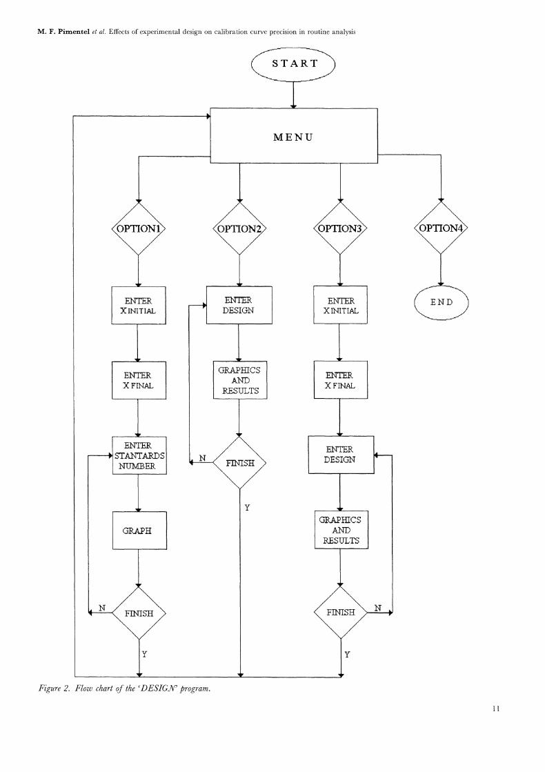
DESIGN was written in the MATLAB high-level lan-guage and was designed to be user-friendly; a flow chartof the program is shown in figure 2. Three options allowevaluation of different experimental designs in fittinglinear models:

(1) Selection of the number of standard solutions, takinginto account the width of the confidence interval forthe D-optimized design.

(2) Selection of the concentration levels (number andlocation).

(3) Comparison of several designs.

In option 1, the user evaluates the effect of the number ofstandard solutions used for calibration, from plots ofconfidence intervals for D-optimized designs. The pro-gram asks for the lower and higher concentrations of theworking range, and the number of standard solutions ofthe design.

Once the number of standard solutions is chosen, option2 permits the effect of the number and distribution ofconcentration levels on the calibration curve to be esti-mated. Efficiencies and plots of confidence intervals forselected designs are given. Since this option is intended toaccess only the effect of how many and which levelsshould be selected, all designs must have the same lowerand higher concentrations, in addition to the samenumber of standard solutions.

In option 3, there is no constraint on the designs undercomparison. Designs with different numbers of standardsolutions, different numbers of concentration levels ordifferent working ranges are evaluated through confi-dence interval plots. The concentration range shown onthe plot is chosen by the user.

The subprogram used to calculate confidence intervalsand efficiencies is described in listing in the Appendix tothis paper.

Simulations

Two practical examples were used to demonstrate the useof the options in the DESIGN program: the determina-tion of potassium and iron in drinking water by flameemission spectroscopy (FES) and inductively-coupledplasma atomic emission spectrometry (ICP-AES), re-

spectively. For both cases a calibration curve needs tobe constructed relating the intensity of the measuredsignal (dependent variable y) to the concentration ofthe analyte in the sample (independent variable x).

It is important to bear in mind that replicate levelsrequire full authentic replicate determinations, and notjust replicated measurements of the same solution.

10


MENU

ENTER?(INITIAL

ENIRX FINAL

ENRSTANTARDSNUIVfBER

ENTERDESIGN

GRAPI-tICSAND

RESULTS

ENTERXINITIAL

ENTERDESIGN

Figure 2. Flow chart of the ’DESIGN’ program.

GR.A.PHICS

RESULTS

Ii


a .-------

b

----_________________

concentration

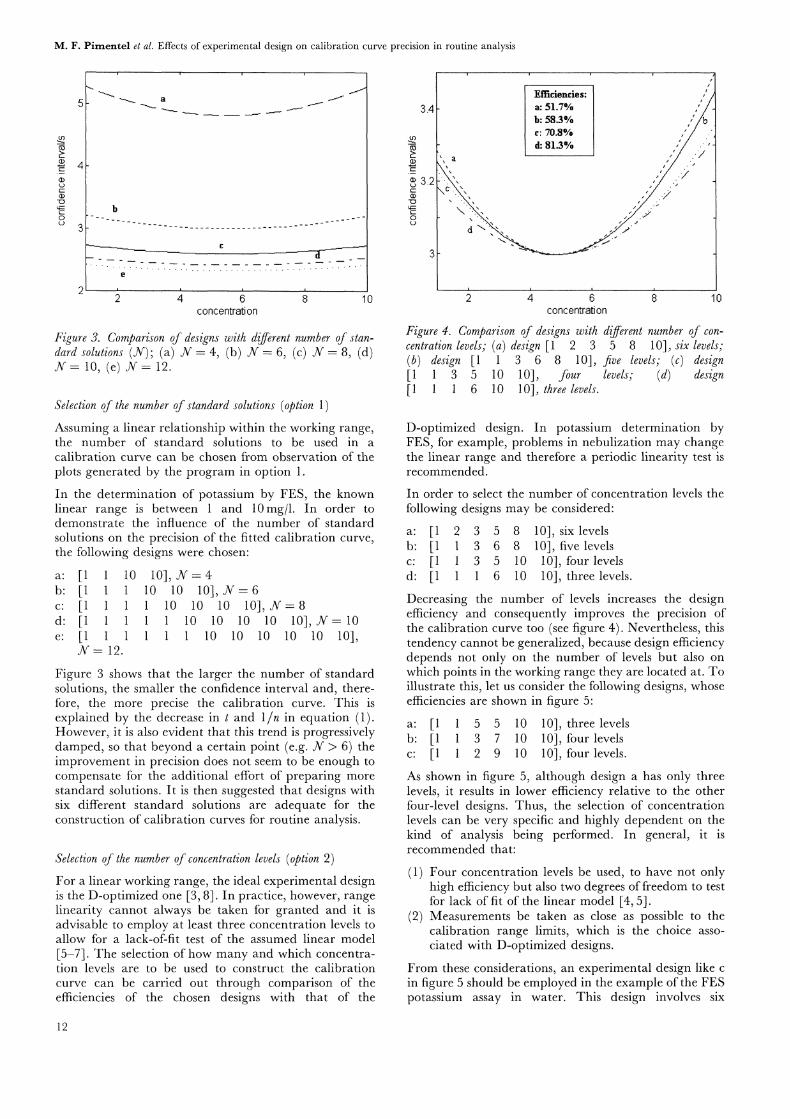
Figure 3. Comparison of designs with different number of stan-dard solutions (N); (a)N- 4, (b)N--6, (c)N- 8, (d)N- 10, (e) N- 12.

Selection of the number of standard solutions (option

Assuming a linear relationship within the working range,the number of standard solutions to be used in acalibration curve can be chosen from observation of theplots generated by the program in option 1.

In the determination of potassium by FES, the knownlinear range is between and 10mg/1. In order todemonstrate the influence of the number of standardsolutions on the precision of the fitted calibration curve,the following designs were chosen:

a: [1b: [1c: [1d: [1e: [1

JV= 12.

10 10],N--410 10 10],N=6

10 10 10 10],N-810 10 10 10 10],N= 10

10 10 10 10 10 10],

Figure 3 shows that the larger the number of standardsolutions, the smaller the confidence interval and, there-fore, the more precise the calibration curve. This isexplained by the decrease in and 1In in equation (1).However, it is also evident that this trend is progressivelydamped, so that beyond a certain point (e.g. N > 6) theimprovement in precision does not seem to be enough tocompensate for the additional effort of preparing morestandard solutions. It is then suggested that designs withsix different standard solutions are adequate for theconstruction of calibration curves for routine analysis.

Selection of the number of concentration levels (option 2)

For a linear working range, the ideal experimental designis the D-optimized one [3, 8]. In practice, however, rangelinearity cannot always be taken for granted and it isadvisable to employ at least three concentration levels toallow for a lack-of-fit test of the assumed linear model[5-7]. The selection of how many and which concentra-tion levels are to be used to construct the calibrationcurve can be carried out through comparison of theefficiencies of the chosen designs with that of the

Efficiencies:"’]

3.4 a: 51.7%b: 58.3% ’"c’ 70.8%

-> a

d: 81.3% ,’"’ .;""’/-eo,_..e 3.2 ’,d """ ".,-,"’

3

concentration

Figure 4. Comparison of designs with different number of con-centration levels; (a) deskn [1 2 3 5 8 10], six levels;(b) design [1 3 6 8 10], five levels; (c) design[1 3 5 10 10], four levels; (d) design[1 6 10 10] three levels.

D-optimized design. In potassium determination byFES, for example, problems in nebulization may changethe linear range and therefore a periodic linearity test isrecommended.

In order to select the number of concentration levels thefollowing designs may be considered:

a: [1 2 3 5 8 10] six levelsb: [1 3 6 8 10] five levelsc: [1 3 5 10 10], four levelsd: [1 6 10 10], three levels.

Decreasing the number of levels increases the designefficiency and consequently improves the precision ofthe calibration curve too (see figure 4). Nevertheless, thistendency cannot be generalized, because design efficiencydepends not only on the number of levels but also onwhich points in the working range they are located at. Toillustrate this, let us consider the following designs, whoseefficiencies are shown in figure 5:

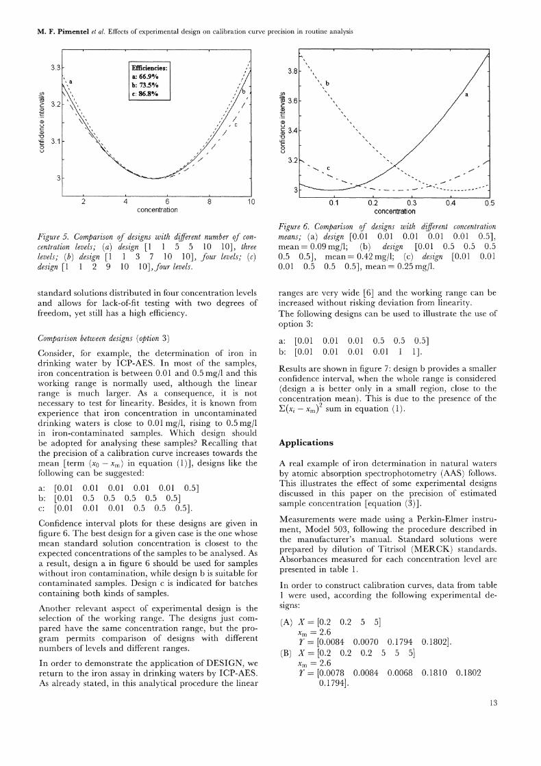
a: [1 5 5 10 10], three levelsb: [1 3 7 10 10] four levelsc: [1 2 9 10 10] four levels.

As shown in figure 5, although design a has only threelevels, it results in lower efficiency relative to the otherfour-level designs. Thus, the selection of concentrationlevels can be very specific and highly dependent on thekind of analysis being performed. In general, it isrecommended that:

(1) Four concentration levels be used, to have not onlyhigh efficiency but also two degrees of freedom to testfor lack of fit of the linear model [4, 5].

(2) Measurements be taken as close as possible to thecalibration range limits, which is the choice asso-ciated with D-optimized designs.

From these considerations, an experimental design like cin figure 5 should be employed in the example of the FESpotassium assay in water. This design involves six

12


3.3

3.2

3.1

concentration

Figure 5. Comparison of designs with different number of con-centration levels; (a) design [1 5 5 10 10], threelevels; (b)design [1 3 7 10 10], four levels; (c)design [1 2 9 10 10],f0ur levels.

3.8

t 3.6

.__3.4

O

3.2

3

", b

a

",,,,,

0 .1 0’.2 0’.3 0’.4 0.5concentration

Figure 6. Comparison of designs with different concentrationmeans; (a) design [0.01 0.01 0.01 0.01 0.01 0.5],mean= 0.09mg/1; (b) design [0.01 0.5 0.5 0.50.5 0.5], mean= 0.42mg/1; (c) design [0.01 0.010.01 0.5 0.5 0.5], mean= 0.25mg/1.

standard solutions distributed in four concentration levelsand allows for lack-of-fit testing with two degrees offreedom, yet still has a high efficiency.

Comparison between designs (option 3)

Consider, for example, the determination of iron indrinking water by ICP-AES. In most of the samples,iron concentration is between 0.01 and 0.5 mg/1 and thisworking range is normally used, although the linearrange is much larger. As a consequence, it is notnecessary to test for linearity. Besides, it is known fromexperience that iron concentration in uncontaminateddrinking waters is close to 0.01 mg/1, rising to 0.5 mg/1in iron-contaminated samples. Which design shouldbe adopted for analysing these samples? Recalling thatthe precision of a calibration curve increases towards themean [term (x0- Xm) in equation (1)], designs like thefollowing can be suggested:

a: [0.01 0.01 0.01 0.01 0.01 0.5]b: [0.01 0.5 0.5 0.5 0.5 0.5]c" [0.01 0.01 0.01 0.5 0.5 0.5].Confidence interval plots for these designs are given infigure 6. The best design for a given case is the one whosemean standard solution concentration is closest to theexpected concentrations of the samples to be analysed. Asa result, design a in figure 6 should be used for sampleswithout iron contamination, while design b is suitable forcontaminated samples. Design c is indicated for batchescontaining both kinds of samples.

Another relevant aspect of experimental design is theselection of the working range. The designs just com-pared have the same concentration range, but the pro-gram permits comparison of designs with differentnumbers of levels and different ranges.

In order to demonstrate the application of DESIGN, wereturn to the iron assay in drinking waters by ICP-AES.As already stated, in this analytical procedure the linear

ranges are very wide [6] and the working range can beincreased without risking deviation from linearity.The following designs can be used to illustrate the use ofoption 3:

a: [0.01 0.01 0.01 0.5 0.5 0.5]b: [0.01 0.01 0.01 0.01 1].

Results are shown in figure 7: design b provides a smallerconfidence interval, when the whole range is considered(design a is better only in a small region, close to theconcentration mean). This is due to the presence of theY](X Xm) sum in equation (1).

Applications

A real example of iron determination in natural waters

by atomic absorption spectrophotometry (AAS) follows.This illustrates the effect of some experimental designsdiscussed in this paper on the precision of estimatedsample concentration [equation (3)].

Measurements were made using a Perkin-Elmer instru-ment, Model 503, following the procedure described inthe manufacturer’s manual. Standard solutions wereprepared by dilution of Titrisol (MERCK) standards.Absorbances measured for each concentration level arepresented in table 1.

In order to construct calibration curves, data from tablewere used, according the following experimental de-

signs"

(A) X=[0.2 0.2 5 5]Xm 2.6Y [0.0084 0.0070x=[o.2 0.2 0.2Xm 2.6Y [0.0078 0.0084

0.1794].

0.1794 0.1802].5 5 5]

0.0068 0.1810 0.1802

13


(c) x=[0. 0. 0.Xm 2.6r [0.0068 0.0088

0.1810 0.1802(D) X=[O. 0. 0.

Xm--r= [0.0088 0.0078

0.180].(E) =[0. 5 5 5

Xm 4.2r [0.0078 0.794

0.80].(F) =[0. B

Xm 2.6r [0.0078 0.0358

0.80].(c) =[0. 0. 0.5

Xm 2.6r [0.0078 0.0084

0.1794].8.25

0. 5 5 5 5]

0.0070 0.0084800].

0. 0. 5]

0.1794

0.0068 0.0070 0.0084

5 5]

0.1800 0.1814 0.1802

4.2 5]

0.0732 0.1098 0.1520

4.6 5 5]

0.00178 0.1668 0.1802

3.2

o 3.05

2.95 ’0"1 0 2 0 3 0.4 0 5concentration

Figure 7. Comparison of designs with different calibrationranges; (a) design [0.01 0.01 0.01 0.5 0.5 0.5]; (b)design [0.01 0.01 0.01 0.01 1].

Table 1. Absorbance values of stan-dard solutions of iron. The repeatedconcentration values correspond toauthentic replicates of the standardsolutions series.

Concentration (mg/1) Absorbance

0.2 0.0078O.2 O.OO88O.2 O.OO68O.2 O.O07OO.2 O.OO840.5 0.01781.0 0.03582.0 O.07323.0 0.10984.2 0.16685.0 0.17945.0 0.18005.0 0.18145.0 0.18025.0 0.1810

Table 2. Estimated values of the ironconcentration (in mg/l) and 95% con-

fidence interval in a sample of wellwater.

Design Estimated concentration

A 0.209 + 0.117B 0.209 :t: 0.071C 0.209 + 0.061D 0.209 + 0.068E 0.209 + 0.087F 0.209 -t- 0.075G 0.209 + 0.072

It is important to note that the estimates of bl and s inequation (3) are approximated to 0.0359 and 0.0008,respectively, for curves A-G above. Hence, confidenceintervals will only depend on the terms related to

experimental design It, n and X, in equation (3)].

The absorbance measured for a sample of well water was0.0081 absorbance units. The estimated concentrationand the 95% confidence intervals around this estimatefor curves A-G are presented in table 2. Some of thefeatures discussed in the previous section are highlightedby table 2:

(1) When the number of standard solutions increasesfrom four (design A) to six (design B), the width ofthe confidence interval decreases 39% (from 0.117 to0.071 mg/1). When the number of standard solutionsgoes from six to eight, the same interval decreasesonly by 14% (from 0.071 to 0.061 mg/1). This smalldecrease needs to be weighed against the task ofpreparing two more standard solutions to decidewhether the increase in precision is worth the trouble.

(2) Designs B, F and G illustrate the effect of the numberof concentration levels. Among these, the D-opti-mized design B presents the narrowest confidenceinterval, but design G, with four levels close to thelimits of the working range, presents practically an

equal interval (table 2).(3) Designs D and E demonstrate how a shift in the

average concentration (Xm) affects the precision ofthe calibration curve. With design D, Xm andwith design E, Xm 4.2. Because the estimatedconcentration [(x0)l=0.209mg/1] is nearer to

Xm than to Xm 4.2, design D shows narrowerconfidence intervals for this estimate (0.068, table 2).This interval is slightly smaller than the D-optimizedone (B), with the same number of standard solutions(0.071, table 2).

Experimental design, of course, varies from case to caseand only the user is able to decide which design is the bestfor any particular situation.

Conclusion

The DESIGN computational program presented in thiswork is conceived as a tool for the experimental designneeded in building calibration curves. It is very simple to

14


use and allows the experimenter to choose among severaloptions.

It is hoped that this program will stimulate analyticalchemists to adopt the practice of planning their experi-ments as a matter of routine.

Acknowledgement

Partial support of CNPq is greatly appreciated.

Appendix

%**SUBROUTINE FOR COMPUTATION OF CON-FIDENCE INTERVALS AND EFFICIENCIES**%X Design vectortam length (X);%****Computation of t-student (95% confidence)****gral (tam-2);t5= 2.282 ./(gral .^5);t4 =0.381 ./(gral .^4);t3 2.9333 ./(gral .^3);t2 2.77608./(gral. 2);tl =2.37286 ./gral;t= (1.95997 + t5 + t4 + t3 + t2 + tl);%****Creating D-optimized design matrix ****Xinic min (X);Xfin max(X);nm round (tam/2);for l:nm

Xotimt(i) Xinic;endfor (nm + 1): tam

Xotimt(i) Xfin;end

%****Confidence intervals computation****

pass abs((Xfin-Xinic) ./500);Xotim Xotimt;um= ones (size (Xotim));Xotimaju =[um Xotim];mato Xotimaju*Xotimaju;invmato inv(mato);pontos Xinic: pass: Xfin;np length(pontos);Xajun =[um X];matn Xajun’*Xajun;invmatn inv(matn);for i= l:np

Xo= [1 pontos(i)];intvoqst(i) Xo*invmato*Xo;intvqstn(i) Xo*invmatn*Xo;

intvstn(i) sqrt(1 + intvqstn(i));intvost(i) sqrt(1 + intvoqst(i));

end

intvo .*intvost;intvn .*intvstn;

%****Efficience computation****Eficiencian (det(matn) ./det(mato))* 100;

References

1. AARONS, L., 1981, Analyst, 106, 1249.2. Box, G. E. E, HUNTER, W. G. and HUNTER, J. S., 1987, Statistics for

Experiments (New York: John Wiley).3. WOLTERS, R. and KATEMAN, G., 1990, Journal of Chernnornetrics, 4,

171.4. MERMET, J. M., 1994, Spectrochirnica Acta, 12-14, 49B, 1313.5. PIMENTEL, M. E and NETO, B. B., 1996, Quimica Nova, 13, 3, 268.6. DRAPER, N. U. and SMITH, H., 1981, Applied Regression Analysis

(New York: John Wiley).7. MONTGOMERY, D. and PECI, E. A., 1982, Introduction to Linear

Regression Analysis (New York: John Wiley).8. ST. JOHN, R. C. and DIAPER, N. R., 1975, Technnometrics, 17, 15.

15

Submit your manuscripts athttp://www.hindawi.com

Hindawi Publishing Corporationhttp://www.hindawi.com Volume 2014

Inorganic ChemistryInternational Journal of

Hindawi Publishing Corporation http://www.hindawi.com Volume 2014

International Journal ofPhotoenergy


Carbohydrate Chemistry

International Journal of


Journal of

Chemistry


Advances in

Physical Chemistry

Hindawi Publishing Corporationhttp://www.hindawi.com

Analytical Methods in Chemistry

Journal of

Volume 2014

Bioinorganic Chemistry and ApplicationsHindawi Publishing Corporationhttp://www.hindawi.com Volume 2014

SpectroscopyInternational Journal of


The Scientific World JournalHindawi Publishing Corporation http://www.hindawi.com Volume 2014

Medicinal ChemistryInternational Journal of


Chromatography Research International


Applied ChemistryJournal of



Theoretical ChemistryJournal of


Journal of

Spectroscopy

Analytical ChemistryInternational Journal of


Journal of


Quantum Chemistry


Organic Chemistry International

ElectrochemistryInternational Journal of

Hindawi Publishing Corporation http://www.hindawi.com Volume 2014


CatalystsJournal of

Documents

tion curve precision in routine analysis