Embed Size (px)
Citation preview
Lexical Semantic Relatedness and Its Application in
Natural Language Processing
by
Alexander Budanitsky
Technical Report CSRG-390
August 1999
Computer Systems Research Group
University of Toronto
Copyright c 1999 by Alexander Budanitsky
ftp://ftp.cs.utoronto.ca/csrg-technical-reports/390

ii
Abstract
Lexical Semantic Relatedness and Its Application in Natural Language Processing
Alexander Budanitsky
Department of Computer Science
University of Toronto
August 1999
A great variety of Natural Language Processing tasks, from word sense disambiguation to
text summarization to speech recognition, rely heavily on the ability to measure semantic
relatedness or distance between words of a natural language. This report is a comprehen-
sive study of recent computational methods of measuring lexical semantic relatedness. A
survey of methods, as well as their applications, is presented, and the question of evalua-
tion is addressed both theoretically and experimentally. Application to the speci�c task
of intelligent spelling checking is discussed in detail: the design of a prototype system
for the detection and correction of malapropisms (words that are similar in spelling or
sound to, but quite di�erent in meaning from, intended words) is described, and results
of experiments on using various measures as plug-ins are considered. Suggestions for
research directions in the areas of measuring semantic relatedness and intelligent spelling
checking are o�ered.
iii
Acknowledgements
First and foremost, I must thank my academic advisor, Graeme Hirst, for having provided
a wealth of ideas, constructive feedback, unfailing support, and overall help in all aspects
of this work.
Next in magnitude, I would like to thank Mark Chignell for having taught me ev-
erything I know about statistical analysis and Stephen Green for having shared both his
programing expertise and his actual code.
A considerable portion of this report draws on work of other researchers. Among
them are Reem Al-Halimi, Jay Jiang, Hideki Kozima, Claudia Leacock, Dekang Lin,
Manabu Okumura, Philip Resnik, David St-Onge, and Michael Sussna | all of whom I
thank personally for having entertained my follow-up queries.
Last, but not least, sincere thanks to Melanie Baljko, Philip Edmonds, Christiane
Fellbaum, Sanda Harabagiu, Karen Kukich, and Daniel Marcu for helpful discussions
and encouragement.
For �nancial support, I gratefully acknowledge the Natural Sciences and Engineering
Research Council of Canada, the University of Toronto, and the UofT Department of
Computer Science.
iv
Contents
1 Introduction 1
1.1 Background and Motivation . . . . . . . . . . . . . . . . . . . . . . . . . 1
1.2 A Word on Terminology and Notation . . . . . . . . . . . . . . . . . . . 3
2 Recent Approaches to Measuring Semantic Relatedness 5
2.1 Dictionary-Based Approaches . . . . . . . . . . . . . . . . . . . . . . . . 5
2.1.1 Background . . . . . . . . . . . . . . . . . . . . . . . . . . . . . . 5
2.1.2 Kozima and Furugori's Spreading Activation on an English Dictio-
nary . . . . . . . . . . . . . . . . . . . . . . . . . . . . . . . . . . 6
2.1.3 Kozima and Ito's Adaptive Scaling of the Semantic Space . . . . . 10
2.2 Thesaurus-Based Approaches . . . . . . . . . . . . . . . . . . . . . . . . 12
2.2.1 Background . . . . . . . . . . . . . . . . . . . . . . . . . . . . . . 12
2.2.2 Morris and Hirst's Algorithm . . . . . . . . . . . . . . . . . . . . 13
2.2.3 Okumura and Honda's Algorithm . . . . . . . . . . . . . . . . . . 14
2.3 Approaches Using a Semantic Network . . . . . . . . . . . . . . . . . . . 15
2.3.1 Background . . . . . . . . . . . . . . . . . . . . . . . . . . . . . . 15
2.3.1.1 Noun Portion of WordNet . . . . . . . . . . . . . . . . . 15
2.3.2 Computing Path Length . . . . . . . . . . . . . . . . . . . . . . . 17
2.3.2.1 Rada et al.'s Simple Edge Counting . . . . . . . . . . . . 17
2.3.2.2 Hirst and St-Onge's Medium-Strong Relations . . . . . . 18
v
2.3.3 Scaling the Network . . . . . . . . . . . . . . . . . . . . . . . . . 20
2.3.3.1 Sussna's Depth-Relative Scaling . . . . . . . . . . . . . . 20
2.3.3.2 Wu and Palmer's Conceptual Similarity . . . . . . . . . 21
2.3.3.3 Leacock and Chodorow's Normalized Path Length . . . 22
2.3.3.4 Agirre and Rigau's Conceptual Density . . . . . . . . . . 23
2.4 Integrated Approaches . . . . . . . . . . . . . . . . . . . . . . . . . . . . 26
2.4.1 Resnik's Information-Based Approach . . . . . . . . . . . . . . . . 26
2.4.2 Jiang and Conrath's Combined Approach . . . . . . . . . . . . . . 28
2.4.3 Lin's Universal Similarity Measure . . . . . . . . . . . . . . . . . 31
3 Comparison with Human Judgement 33
3.1 Assessing Measures of Semantic Relatedness . . . . . . . . . . . . . . . . 33
3.2 The Data . . . . . . . . . . . . . . . . . . . . . . . . . . . . . . . . . . . 34
3.3 The Results . . . . . . . . . . . . . . . . . . . . . . . . . . . . . . . . . . 35
3.3.1 Discussion . . . . . . . . . . . . . . . . . . . . . . . . . . . . . . . 35
4 Some Applications and Relevant Results 47
4.1 Resolution of Word Sense Ambiguity . . . . . . . . . . . . . . . . . . . . 47
4.1.1 Agirre and Rigau . . . . . . . . . . . . . . . . . . . . . . . . . . . 48
4.1.2 Sussna . . . . . . . . . . . . . . . . . . . . . . . . . . . . . . . . . 50
4.1.3 Leacock and Chodorow . . . . . . . . . . . . . . . . . . . . . . . . 51
4.1.4 Lin . . . . . . . . . . . . . . . . . . . . . . . . . . . . . . . . . . . 55
4.1.5 Okumura and Honda . . . . . . . . . . . . . . . . . . . . . . . . . 57
4.2 Identifying the Discourse Structure . . . . . . . . . . . . . . . . . . . . . 58
4.2.1 Okumura and Honda . . . . . . . . . . . . . . . . . . . . . . . . . 58
4.2.2 Morris and Hirst . . . . . . . . . . . . . . . . . . . . . . . . . . . 59
4.3 Text Summarization, Annotation, and Indexing . . . . . . . . . . . . . . 60
4.3.1 Barzilay and Elhadad . . . . . . . . . . . . . . . . . . . . . . . . . 60
vi
4.3.2 Green . . . . . . . . . . . . . . . . . . . . . . . . . . . . . . . . . 62
4.3.3 Kazman et al. . . . . . . . . . . . . . . . . . . . . . . . . . . . . . 65
4.4 Lexical Selection . . . . . . . . . . . . . . . . . . . . . . . . . . . . . . . 67
4.4.1 Wu and Palmer . . . . . . . . . . . . . . . . . . . . . . . . . . . . 67
4.5 Information Retrieval . . . . . . . . . . . . . . . . . . . . . . . . . . . . . 68
4.5.1 Rada et al. . . . . . . . . . . . . . . . . . . . . . . . . . . . . . . 68
4.5.2 Richardson and Smeaton . . . . . . . . . . . . . . . . . . . . . . . 69
4.6 Word Prediction . . . . . . . . . . . . . . . . . . . . . . . . . . . . . . . . 70
4.6.1 Kozima and Ito . . . . . . . . . . . . . . . . . . . . . . . . . . . . 70
5 Malapropism Correction in Free Text 73
5.1 Automatic Spelling Correction . . . . . . . . . . . . . . . . . . . . . . . . 73
5.2 Previous Work in Malapropism Correction . . . . . . . . . . . . . . . . . 76
5.3 The New Algorithm . . . . . . . . . . . . . . . . . . . . . . . . . . . . . . 78
5.3.1 Introductory Remarks . . . . . . . . . . . . . . . . . . . . . . . . 78
5.3.2 Algorithm Overview . . . . . . . . . . . . . . . . . . . . . . . . . 79
5.3.3 Details of the Algorithm . . . . . . . . . . . . . . . . . . . . . . . 83
5.3.3.1 The Term Data Structure . . . . . . . . . . . . . . . . . 83
5.3.3.2 Named Entities . . . . . . . . . . . . . . . . . . . . . . . 84
5.3.3.3 Compounds . . . . . . . . . . . . . . . . . . . . . . . . . 84
5.3.3.4 Alternative Lemmas . . . . . . . . . . . . . . . . . . . . 85
5.3.3.5 Search for Relatives . . . . . . . . . . . . . . . . . . . . 86
5.3.3.6 Semantic Distance Between Terms . . . . . . . . . . . . 87
5.3.3.7 Pruning . . . . . . . . . . . . . . . . . . . . . . . . . . . 88
5.3.3.8 Spelling Variations . . . . . . . . . . . . . . . . . . . . . 90
5.3.3.9 Alarms and Related Issues . . . . . . . . . . . . . . . . . 90
5.4 System Parameters . . . . . . . . . . . . . . . . . . . . . . . . . . . . . . 91
5.4.1 Measures of Semantic Distance . . . . . . . . . . . . . . . . . . . 91
vii
5.4.1.1 Distance vs Relatedness . . . . . . . . . . . . . . . . . . 92
5.4.1.2 Implementation Notes . . . . . . . . . . . . . . . . . . . 92
5.4.2 Threshold Determination . . . . . . . . . . . . . . . . . . . . . . . 96
5.4.3 Search Scope . . . . . . . . . . . . . . . . . . . . . . . . . . . . . 99
5.5 Performance Evaluation . . . . . . . . . . . . . . . . . . . . . . . . . . . 100
5.5.1 Some Terminology . . . . . . . . . . . . . . . . . . . . . . . . . . 100
5.5.2 Performance Measures . . . . . . . . . . . . . . . . . . . . . . . . 101
5.6 Analysis of Results . . . . . . . . . . . . . . . . . . . . . . . . . . . . . . 104
5.6.1 Some Examples . . . . . . . . . . . . . . . . . . . . . . . . . . . . 104
5.6.1.1 Performance on Genuine Malapropisms . . . . . . . . . . 104
5.6.1.2 Performance on Non-malapropisms . . . . . . . . . . . . 107
5.6.2 St-Onge's Performance Measures . . . . . . . . . . . . . . . . . . 111
5.6.3 Precision and Recall . . . . . . . . . . . . . . . . . . . . . . . . . 112
6 Conclusion 123
6.1 Measuring Semantic Relatedness . . . . . . . . . . . . . . . . . . . . . . . 123
6.1.1 Summary . . . . . . . . . . . . . . . . . . . . . . . . . . . . . . . 123
6.1.2 Conclusions and Future Directions . . . . . . . . . . . . . . . . . 124
6.2 Detection and Correction of Malapropisms . . . . . . . . . . . . . . . . . 128
6.2.1 Summary . . . . . . . . . . . . . . . . . . . . . . . . . . . . . . . 128
6.2.2 Conclusions and Future Directions . . . . . . . . . . . . . . . . . 129
A Sample Text With Introduced Malapropisms 133
A.1 Text . . . . . . . . . . . . . . . . . . . . . . . . . . . . . . . . . . . . . . 133
viii
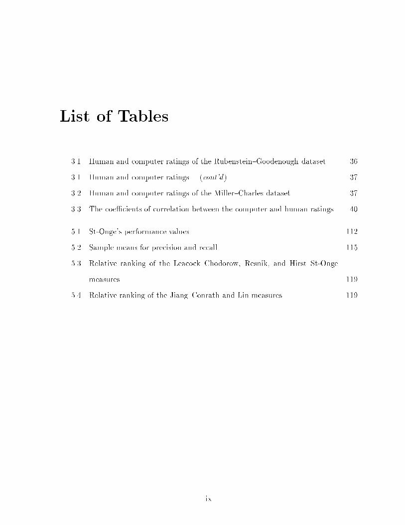
List of Tables
3.1 Human and computer ratings of the Rubenstein{Goodenough dataset. . . 36
3.1 Human and computer ratings. . . (cont'd). . . . . . . . . . . . . . . . . . . 37
3.2 Human and computer ratings of the Miller{Charles dataset. . . . . . . . 37
3.3 The coe�cients of correlation between the computer and human ratings. 40
5.1 St-Onge's performance values. . . . . . . . . . . . . . . . . . . . . . . . . 112
5.2 Sample means for precision and recall. . . . . . . . . . . . . . . . . . . . 115
5.3 Relative ranking of the Leacock{Chodorow, Resnik, and Hirst{St-Onge
measures. . . . . . . . . . . . . . . . . . . . . . . . . . . . . . . . . . . . 119
5.4 Relative ranking of the Jiang{Conrath and Lin measures. . . . . . . . . . 119
ix

x
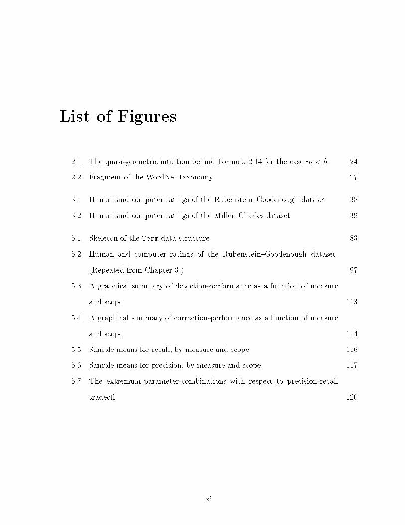
List of Figures
2.1 The quasi-geometric intuition behind Formula 2.14 for the case m < h. . 24
2.2 Fragment of the WordNet taxonomy. . . . . . . . . . . . . . . . . . . . . 27
3.1 Human and computer ratings of the Rubenstein{Goodenough dataset. . . 38
3.2 Human and computer ratings of the Miller{Charles dataset. . . . . . . . 39
5.1 Skeleton of the Term data structure. . . . . . . . . . . . . . . . . . . . . . 83
5.2 Human and computer ratings of the Rubenstein{Goodenough dataset.
(Repeated from Chapter 3.) . . . . . . . . . . . . . . . . . . . . . . . . . 97
5.3 A graphical summary of detection-performance as a function of measure
and scope. . . . . . . . . . . . . . . . . . . . . . . . . . . . . . . . . . . . 113
5.4 A graphical summary of correction-performance as a function of measure
and scope. . . . . . . . . . . . . . . . . . . . . . . . . . . . . . . . . . . . 114
5.5 Sample means for recall, by measure and scope. . . . . . . . . . . . . . . 116
5.6 Sample means for precision, by measure and scope. . . . . . . . . . . . . 117
5.7 The extremum parameter-combinations with respect to precision-recall
tradeo�. . . . . . . . . . . . . . . . . . . . . . . . . . . . . . . . . . . . . 120
xi

xii
Chapter 1
Introduction
1.1 Background and Motivation
Is �rst related to �nal? Is hair related to comb? Is doctor related to hospital and, if so,
is the connection between them stronger than that between doctor and nurse? In what
sense is virgin related to bush?1 Striving to provide well-justi�ed answers to these ques-
tions are lexical semanticists working in the area ofmeasuring semantic relatedness. Their
main motivation lies in the tremendous applicability of the ability to measure semantic
relatedness to practical tasks involving natural language. In word sense disambiguation,
for instance, the intended sense of a polysemous word can be found by computing the
semantic relatedness of the word in each of its senses to a window of unambiguous words
surrounding it in text and then selecting the sense delivering the highest cumulative
value of the relatedness [Sussna, 1993, Sussna, 1997]. To determine the structure of
a text, the knowledge of what words are semantically related can be used to identify
sequences, or chains, of such related words, which can in turn be used to determine
boundaries between segments of text that form `topical units' (e.g., paragraphs in the
case of transcribed speech) [Morris and Hirst, 1991, Okumura and Honda, 1994]. If one
1We thank Chrysanne DiMarco for suggesting some of these examples.
1
2 Chapter 1. Introduction
is furthermore capable of di�erentiating among word chains on the basis of their strength,
summaries of a given text can be generated by, for instance, extracting text segments cor-
responding to the chains stronger than a certain threshold [Barzilay and Elhadad, 1997].
An obvious use of semantic relatedness in information retrieval is as a replacement for the
conventionally used lexical equivalence: instead of retrieving documents solely on the ba-
sis of occurrence of query terms in them, we could include into consideration documents
containing terms that are semantically related to query terms [Cohen and Kjeldsen, 1987,
Rada and Bicknell, 1989]. In speech and text recognition, the most likely interpretation
of an unrecognizable lexeme can be computed by choosing the candidate most closely
related to a subset of the lexemes recognized earlier.
The problem of formalizing and quantifying the intuitive notion of semantic relat-
edness between lexical units has a long history in philosophy, psychology, and arti�cial
intelligence, going back at least to Aristotle (384{322 b.c.e.).
Among the heralds of the contemporary wave of research are Osgood [1952], Quillian
[1968], and Collins and Loftus [1975]. Osgood's \semantic di�erential" was an attempt
to represent words as entities in an n-dimensional space, where measuring the distance
between them could naturally follow from our knowledge of Euclidean geometry. Unfortu-
nately, after extensive experimentation, Osgood found his system to rely on \connotative
emotions" attached to a word rather than its \denotative meaning" [Kozima and Furu-
gori, 1993] and discontinued further research. The more `procedural' approach of Quillian
and Collins and Loftus, termed \spreading activation", on the other hand, continues to
motivate researchers in lexical semantics still [Hirst, 1987, Kozima and Furugori, 1993,
Kozima and Ito, 1997].
Almost two decades ago, McGill and colleagues [1979] drew up a list of 67 similarity
measures used in information retrieval alone [Lin, 1998]. Research in the �eld has re-
mained active and productive to this day, with the impressive range of applications that
the ability to measure semantic relatedness has found being, as we argued above, the
1.2. A Word on Terminology and Notation 3
principal driving force behind it.
This report is an attempt to survey the current state of a�airs with regard to the
methodology for (Chapter 2) and uses of (Chapter 4) measuring semantic relatedness,
address the question of assessing the `goodness' of a computational measure (Chapters 3
and 5), and suggest directions for future research in the area (Chapter 6).
1.2 A Word on Terminology and Notation
When reviewing literature related to the topic of the report, one can notice at least three
di�erent terms used by di�erent authors or sometimes interchangeably by same authors:
relatedness, similarity, and distance.
Resnik [1995] attempts to demonstrate the distinction between the �rst two by way of
example. \Cars and gasoline", he writes, \would seem to be more closely related than,
say, cars and bicycles, but the latter pair are certainly more similar." Similarity, thus,
represents a special case of relatedness | and this is the perspective we adopt in this
report. Among other relationships that the notion of semantic relatedness encompasses
are the various kinds of meronymy (e.g., window{house, issue{serial publication), antonymy
(hot{cold), and functional association (ocean{cruiser).
The term semantic distance may cause even more confusion, as it can be used when
talking about either similarity or relatedness: two concepts are close to one another if
their similarity or relatedness is high, and they are distant in the opposite case. Further-
more, most of the time, the two uses do not contradict each other. But not always: if
concepts are close if and only if they are similar, concepts must be distant if they are
dissimilar; if, however, similarity is regarded as a generalization of synonymy, then, since
antonymy is a special case of dissimilarity, one could argue that the above relation ceases
to be intuitive, for antonyms are, actually, very close to each other semantically.
We would thus have very much preferred to be able to adhere to the view of semantic
4 Chapter 1. Introduction
distance as the inverse of semantic relatedness, not merely similarity, in the present
report. Unfortunately, because of the sheer number of methods measuring similarity,
as well as those measuring distance as the opposite of similarity, this would have made
for an awkward presentation. Therefore, more due to tradition than common sense, we
have to ask the reader to rely on context when interpreting what exactly the expressions
semantic distance, semantically distant, and semantically close mean in each particular
case.
Various approaches presented below speak of concepts and words. As a means of
acknowledging the polysemy of language, in this report, unless stated otherwise, the
term concept will refer to a particular sense of a given word . In running text, examples
of concepts are typeset in sans serif whereas examples of words are given in italics; and in
formulas, concepts and words will usually be denoted by c and w, with various subscripts.
For the sake of uniformity of presentation, we have taken the liberty of altering the original
notation in some formulas accordingly.
Chapter 2
Recent Approaches to Measuring
Semantic Relatedness
2.1 Dictionary-Based Approaches
2.1.1 Background
Dictionaries are perhaps the resource most readily associated with linguistic knowledge
in people's minds. It is therefore not at all surprising that attempts have been made to
adapt dictionaries to the task of measuring semantic distance computationally.
The Longman Dictionary of Contemporary English (LDOCE) was the �rst dictionary
available to researchers in a machine-readable format (on a magnetic tape).1 The struc-
ture of LDOCE, coupled with the cooperation of its publisher, \has made it the most
widely used English dictionary for language processing" [Guthrie et al., 1996].
A remarkable feature of LDOCE, exploited in both works presented in this section,
is its use of a controlled vocabulary in headword de�nitions. The Longman De�ning
Vocabulary (LDV) comprises 2,851 words, chosen on the basis of West's [1953] survey of
1\In return for a carefully worded contract restricting use to research projects and a moderate sumof money" [Evens, 1988].
5
6 Chapter 2. Recent Approaches to Measuring Semantic Relatedness
restricted vocabulary, and each of the dictionary's 56,000 headwords is de�ned in terms
of these words only.2
2.1.2 Kozima and Furugori's Spreading Activation on an En-
glish Dictionary
A well-compiled dictionary may be viewed as a \closed paraphrasing system of natural
language" [Kozima and Furugori, 1993]: each of its headwords is de�ned in terms of
other headwords and/or their derivatives. A natural way of turning a dictionary into
a network is thus to create a node for every headword and link this node to the nodes
corresponding to all the headwords encountered in its de�nition. Having done this, one
will immediately notice that, if the dictionary uses a controlled de�ning vocabulary, it
will correspond to the densest part of the network: the remaining nodes, which represent
the headwords outside of the de�ning vocabulary, can be pictured as being situated at
the fringe of the network, as they are linked only to de�ning-vocabulary nodes and not
to each other.
These observations and the conforming structure of LDOCE underlie Kozima and
Furugori's technique of creating a semantic network from an English dictionary. They
began by extracting from LDOCE only those entries whose headwords belonged to the
LDV. The resulting subdictionary, rendered as s-expressions and namedGloss�eme, con-
tained 2,851 entries comprising 101,861 words (tokens) in all. Each entry of Gloss�eme
was composed of a headword, a word-class (part of speech), and one or more units corre-
sponding to the numbered sense-de�nitions in the respective LDOCE entry. Each unit,
in turn, consisted of a head-part, corresponding to the genus, and one or more det-parts,
corresponding to the di�erentia.
Gloss�eme was subsequently translated into a semantic network named Paradigme.
2The �gures are for the 1987 edition of LDOCE, with which both groups of researchers worked.
2.1. Dictionary-Based Approaches 7
Paradigme spans 2,851 nodes, corresponding to the entries of Gloss�eme, interconnected
by 295,914 unnamed links.
Each node of Paradigme includes a headword, a word-class, and an activity-value
(see below) and is linked to the nodes representing the words in the de�nition of the
Gloss�eme entry to which it corresponds (for the average of approximately 104 links per
node). Links emanating from a given node form two distinct sets: a r�ef�erant and a r�ef�er�e.
The r�ef�erant set is meant to be re ective of the intensions of the node's headword. It
contains several subsets, called subr�ef�erants, each of which corresponds to a Gloss�eme
unit (i.e., its constituent links connect the node to the nodes representing the words in
the unit). We can think of a r�ef�erant as the set of outgoing links of a node. The r�ef�er�e
of a node n, on the other hand, provides information about its extension by linking n to
the nodes that refer to it (in their respective Gloss�eme de�nitions). This group of links
can thus be viewed as incoming.
As a brief illustration, the word red gives rise to two nodes in Paradigme: one for its
adjective (red_1) and the other for its noun senses (red_2). Then, red_1 will have red
as the headword and adj as its word-class. Its second subr�ef�erant, corresponding to the
unit `(of human hair) of a bright brownish orange or copper colour', will include links to
the nodes brown_1 (note the morphological transformation), colour_1, and colour_2.
Its r�ef�er�e, on the other hand, will include a link to apple_1, as the latter has a link to
red_1 in its r�ef�erant.
Finally, a link to node n has thickness tn, computed from the frequency of its headword
wn in Gloss�eme \and other information" and normalized over each subr�ef�erant or r�ef�er�e.
(See [Kozima and Furugori, 1993] for further details.)
Once the network is built, the similarity between words of the LDV can be computed
by means of spreading activation on the network. Each node can hold activity (in its
activity-value �eld), which is received and transmitted through network links. Node n's
8 Chapter 2. Recent Approaches to Measuring Semantic Relatedness
activity value vn(T + 1) at time T + 1 is calculated as follows:
vn(T + 1) = �(Rn(T ) +R0
n(T )
2+ en(T )) ; (2.1)
where Rn(T ) and R0n(T ) are the composite activities, at time T , of the nodes referred to
in n's r�ef�erant and r�ef�er�e, respectively,3 en(T ) is the activity imparted, at time T , onto
n from the outside (see below), and � is a function limiting the output value to [0; 1].4
Activating node n for a period of time t, i.e., letting en(T ) > 0 for T 2 [0; t], causes
the activity to spread over Paradigme. This results in an activated pattern, which, in
Kozima and Furugori's estimates, reaches equilibrium after 10 steps (time units). The
pattern produced by activity that originates at a given node k can be used to assess the
similarity between the node's headword, wk, and any word in the LDV. The algorithm
for computing similarity simKF(wk; wl) between the words wk and wl is as follows:
1. Reset activity-values of all the nodes in the network.
2. Activate node k, corresponding to the word wk, with strength ek = s(wk) for 10
steps to obtain an activated pattern P (wk). Here, s(wk) is the signi�cance of wk,
de�ned as \the normalized information of the word wk" in the 5,487,056-word
corpus [West, 1953].
3. Observe a(P (wk); wl), the activity value of node l in pattern P (wk) (computed,
supposedly, as vl(10); see Equation 2.1). The similarity value sought is then
simKF(wk; wl) = s(wl) � a(P (wk); wl) : (2.2)
For instance, to compute the similarity between the words red and orange, we �rst
induce an activated pattern P (red) on Paradigme. The word signi�cance of red, which
3The values of both Rn(T ) and R0n(T ) depend on the activity values of the members of their respective
sets as well as on the thicknesses of the links involved (see [Kozima and Furugori, 1993] for details). Aninteresting point to note is that the �nal expression for Rn(T ) is given in the paper in terms of \themost plausible subr�ef�erant" of n, which amounts to provisional disambiguation of the word associatedwith the node (see above).
4Kozima and Furugori do not provide a precise formula for computing �.
2.1. Dictionary-Based Approaches 9
appears 2,308 times in the corpus, is computed as
s(red) =� log(2308=5487056)
� log(1=5487056)= 0:500955 :
Since the network contains two nodes with the headword red, both of them are activated
with the strength e = 0:500955. Next, we observe a(P (red); orange) = 0:390774 and
compute s(orange) = 0:676253. According to Equation 2.2 then,
simKF(red; orange) = 0:676253 � 0:390774 = 0:264262 :
The procedure described above de�nes a similarity measure on elements of the LDV,
i.e., simKF : LDV � LDV ! [0; 1],5 which makes up only about 5% of LDOCE. The
natural next step in Kozima and Furugori's research was, therefore, to try and extend
the measure to simKF : LDOCE�LDOCE! [0; 1]. This was accomplished indirectly by
extending simKF of Equation 2.2 to simKF : LDVn � LDVm ! [0; 1], where n and m are
essentially arbitrary positive integers: any word in the LDOCE-complement of the LDV
was treated as a list W = fw1; : : : ; wrg of the words in its de�nition, with the similarity
between word lists W;W 0 de�ned as
simKF(W;W0) = (
Xw02W 0
s(w0) � a(P (W ); w0)) : (2.3)
Here, P (W ) is the pattern resulting from the activation of each wi 2 W with strength
s(wi)2=Ps(wk) for 10 steps,6 and is a function limiting the output value to [0; 1].7
An example of applying formula 2.3 is arriving at the similarity value of the words
linguistics and stylistics:
simKF(linguistics; stylistics)
= simKF(fthe, study, of, language, in, general, and, of, particular,
5To verify the range, notice that both s(w) and a(P (w0); w00) (Equation 2.2) return values within theinterval [0; 1].
6The signi�cance of a word not found in [West, 1953] was estimated as the average signi�cance of itsword class.
7Again, no explicit formula is given for in [Kozima and Furugori, 1993].
10 Chapter 2. Recent Approaches to Measuring Semantic Relatedness
languages, and, their, structure, and, grammar, and, historyg;
fthe, study, of, style, in, written, or, spoken, languageg)
= 0:140089 :
2.1.3 Kozima and Ito's Adaptive Scaling of the Semantic Space
Fairly soon after coming up with the technique for computing similarity by means of
spreading activation on a dictionary, Kozima and another colleague, Ito [1997], realized
that Kozima and Furugori's [1993] method, as well as those of Osgood [1952], Morris and
Hirst [1991], and others, can be categorized as context-free, or static, for it measures the
distance between words irrespective of context. They then set out to build on the work
of Kozima and Furugori and derive a context-sensitive, or dynamic, measure by taking
into account the \associative direction" for a given word pair.
The motivation behind the newly-proposed method lies in the observations that, when
asked to associate words freely from a given word, \we often imagine a certain context
for retrieving related words", and, if we change context, the perceived distance for the
same word pair will, generally, also change.
In their work, Kozima and Ito represent context by a set C of characteristic words.
For example, C = fcar, busg imposes the associative direction of vehicle (association
sets are then likely to include taxi, railway, airplane, etc.), whereas C = fcar, engineg
imposes the direction of components of car (tire, seat, headlight, etc.). Denoting the given
vocabulary by V , the objective of the method can be expressed as the computation of
distance distKI(w;w0jC) between any two words w;w0 in V \under the context speci�ed
by" C.
The strategy for computing distKI(w;w0jC) is \ `adaptive scaling' of a semantic space"
in which every word in V is represented as a multidimensional vector. Kozima and Ito
adopted LDV as their vocabulary and activated patterns P (w)'s (Section 2.1.2) as their
vectors (activating the node(s) with w as the headword results in a unique equilibrium
2.1. Dictionary-Based Approaches 11
pattern of activity, which admits a trivial vector-representation if we treat the nodes of
Paradigme (Section 2.1.2) as coordinates).
By construction, P (w) represents the meaning of w through its relationship with the
rest of V . The geometric distance between P (w) and P (w0) is then indicative of the
semantic distance between w and w0 | but it is also static. To provide for context-
sensitive distance, P-vectors are �rst transformed into Q-vectors by means of principal
component analysis. A new set of axes X = fX1; : : : ;X2851g is computed in such a
way that it provides an orthonormal coordinate system for P-vectors, and the axes are
arranged in descending order of P-vector variance. Then, the �rst m axes X1; : : : ;Xm
(see below) are selected, and every P (wi) is projected onto each of them. Finally, the
projected vectors are `centered' so that their `mean vector' is 0.
Since the variance for each axis \indicates the amount of information represented
by" that axis, the axes in X are arranged in \descending order of their signi�cance".
Plotting the cumulative variance against m shows that even a couple of hundred axes
can account for nearly half of the \total information of P-vectors". The exact value of
m = 281 is obtained by choosing m, 1 � m � 2851, resulting in minimal noise (where
noise is estimated byP
w2F jQ(w)j with F being the set of all function words in V ).
Thus, principal component analysis both compresses semantic information (by reducing
the number of dimensions of the vector space) and reduces the amount of noise present.
Because, as is demonstrated in the paper, semantically related words have close
(\similar") P-vectors and since principal component analysis preserves relative distance,
in a semantic subspace of Q-vectors with appropriately chosen dimensions words that
are related should form clusters. It is the selection of appropriate dimensions (axes)
that is accomplished by adaptive scaling. The semantic space is altered (\scaled up or
down") so as to make the words in C = fw1; : : : ; wng close to one another. The distance
distKI(w;w0jC) between two words w and w0 (with the corresponding Q(w) = (q1; : : : ; qm)
12 Chapter 2. Recent Approaches to Measuring Semantic Relatedness
and Q(w0) = (q01; : : : ; q0m)) is computed as
distKI(w;w0jC) =
vuut mXi=1
(fi(qi � q0i))2 : (2.4)
Each fi 2 [0; 1] in the equation is a scaling factor, de�ned as
fi =
8><>:
1� ri; ri � 1
0; ri > 1: (2.5)
Here,
ri = SDi(C)=SDi(V ) ; (2.6)
where SDi(C) is, in turn, the standard deviation of the words in C projected onto Xi
and SDi(V ) is that of the words in V .
If C forms a compact cluster on Xi, the latter becomes a signi�cant axis (i.e., fi � 1),
and it becomes insigni�cant (fi � 0) if C does not form an \apparent cluster" on Xi.
Hence, the process of adaptive scaling \tunes" the distance between Q-vectors to a given
word set C, thereby making it context-sensitive. Such a tune-up is not computationally
expensive, since the fi's are the only parameters that change from one context set to
another.
2.2 Thesaurus-Based Approaches
2.2.1 Background
Since both approaches described in this section make use of a Roget's-type thesaurus, we
shall make a couple of remarks about this knowledge source.
Conceived by Peter Mark Roget over 150 years ago, the thesaurus has developed into
a massive classi�cation of words and phrases around ideas and concepts. The levels of
thesaural hierarchy referred to below include classes, categories, and subcategories. An
essential feature of the thesaurus is its index, which contains category numbers along
2.2. Thesaurus-Based Approaches 13
with labels representative of those categories for each word. Cross-referencing among
categories is accomplished with the aid of pointers.
As Morris points out, \the thesaurus simply groups words by idea" [Morris, 1988].
In contrast with traditional AI knowledge bases, the thesaurus \does not have to name
or classify the idea"; it merely groups related words without attempting to explicitly
indicate how and why they are related. Another notable distinction is the following.
While, in frame systems or semantic networks, concepts \that are related are actually
physically close in the representation . . . this need not be true" in a thesaurus. \Physical
closeness has some importance . . . but words in the index of the thesaurus often have
widely scattered categories, and each category often points to a widely scattered selection
of categories."
In part as a consequence of the structure of the thesaurus, no numerical value for
semantic distance can typically be obtained: rather, algorithms using the thesaurus
compute a distance implicitly and return a boolean value of `close' or `not close'.
2.2.2 Morris and Hirst's Algorithm
Working with an abridged version of Roget's Thesaurus, Morris and Hirst [1991] identi�ed
�ve types of semantic relations between words. In their approach, two words were deemed
to be related to one another, or semantically close, if their base forms satisfy any one of
the following conditions:
1. they have a category in common in their index entries;
2. one has a category in its index that contains a pointer to a category of the other;
3. one is either a label in the other's index entry or is in a category of the other;
4. they are both contained in the same subcategory;
5. they both have categories in their index entries that point to a common category.
14 Chapter 2. Recent Approaches to Measuring Semantic Relatedness
These relations account for such pairings as wife and married, car and driving, blind and
see, reality and theoretically, brutal and terri�ed.
Of the �ve types of relations, perhaps the most intuitively plausible ones | namely,
the �rst two in the list above | were found to validate over 90% of the intuitive lexical re-
lationships that the authors used as a benchmark in their experiments (see Section 4.2.2).
In addition to the �ve relations presented so far, two words with identical base forms
were, naturally, also considered related. Less trivially, Morris and Hirst came to allow
one transitive link with respect to their relation set. That is, if word w1 is related to
word w2, word w2 is related to word w3, and word w3 is related to word w4, then w1
would be considered related to word w3 but not to word w4. The introduction of limited
transitivity of this kind enabled the authors to relate, for instance, afraid to uneasily
through trouble.
Morris and Hirst used their metric for \identifying and tracing patterns of lexical
cohesion" (termed lexical chains) in free-running text, as will be discussed later in the
report.
2.2.3 Okumura and Honda's Algorithm
Morris and Hirst's work on use of thesaurus for analyzing lexical cohesion in English
inspired Okumura and Honda's investigation into construction and applications of lexical
chains for Japanese [Okumura and Honda, 1994].
As far as the determination of word relatedness is concerned, Okumura and Honda's
method can be regarded as a restriction of Morris and Hirst's: while they use the Japanese
thesaurus Bunrui-goihyo, which is similar to Roget's, only the �rst of the �ve relations
listed in the previous subsection is considered su�cient for a pair of words to be related.
We will have more to say about Okumura and Honda's work when we talk about
applications in Chapter 4.
2.3. Approaches Using a Semantic Network 15
2.3 Approaches Using a Semantic Network
2.3.1 Background
According to Lee et al. [1993], a \semantic network is broadly described as any repre-
sentation interlinking nodes with arcs, where the nodes are concepts and the links are
various kinds of relationships between concepts."
The majority of the methods discussed in the present and the following section use
WordNet [Miller et al., 1990, Fellbaum, 1998], a broad coverage semantic network created
as an attempt \to model the lexical knowledge of a native speaker of English" [Richard-
son and Smeaton, 1995a]. English nouns, verbs, adjectives, and adverbs are organized
into synonym sets (synsets), each representing one underlying lexical concept, that are
interlinked with a variety of relations.
2.3.1.1 Noun Portion of WordNet
The noun portion of WordNet has fairly rich connectivity and remains by far the most
developed part of the network. Its more than 60,500 synsets, representing over 107,400
noun senses, are linked by over 150,000 arcs of nine types corresponding to the nine
relations adopted by WordNet's creators (see below).8
The subsumption hierarchy (hypernymy/hyponymy) constitutes the backbone of the
noun subnetwork, accounting for close to 80% of the links. At the top of the hierarchy
are 11 abstract concepts, termed unique beginners, such as entity (`something having
concrete existence; living or nonliving'), psychological feature (`a feature of the mental
life of a living organism'), abstraction (`a concept formed by extracting common features
from examples'), shape/form (`the spatial arrangement of something as distinct from its
substance'), event (`something that happens at a given place and time'), etc. Hence,
strictly speaking, the noun portion consists of eleven separate hierarchies \cover[ing]
8The �gures given throughout this subsection are for version 1.5 of WordNet (March 1995).
16 Chapter 2. Recent Approaches to Measuring Semantic Relatedness
distinct conceptual and lexical domains" [Miller, 1998]. These hierarchies are not entirely
disjoint, however, and do not form trees (i.e., multiple inheritance is allowed). The
maximum depth of the noun hierarchy is 16 nodes.
The nine types of relations de�ned on the noun subnetwork are as follows:
hypernymy: the is-a relation: e.g., plant is a hypernym of tree since tree is-a plant
hyponymy: the subsumes relation (inverse of hypernymy)
meronymy: the set of three relations that can be collectively referred to as part-of:
component-object: e.g., branch is a meronym of tree since branch is a compo-
nent of tree
member-collection: e.g., tree is a meronym of forest since tree is a member of
forest
stu�-object: e.g., aluminum is a meronym of airplane since aluminum is the stu�
that airplane is made from
holonymy: the set of three relations that can be collectively referred to as has-a (and
that are the respective inverses of meronymy):
object-component: the inverse of the component-object
collection-member: the inverse of the member-collection
object-stu�: the inverse of the stu�-object
antonymy: very roughly, the complement-of relation (self-inverse): e.g., rise and fall
are antonyms, and so are brother and sister.
For the sake of completeness, we also mention the tenth relation, synonymy, which is
intranode and self-inverse.
2.3. Approaches Using a Semantic Network 17
2.3.2 Computing Path Length
A natural way to evaluate semantic similarity in a taxonomy, given its graphical rep-
resentation, is \to evaluate the distance between the nodes corresponding to the items
being compared | the shorter the path from one node to another, the more similar they
are. Given multiple paths, one takes the length of the shortest one" [Resnik, 1995]. The
�rst approach presented in this section follows exactly this methodology.
2.3.2.1 Rada et al.'s Simple Edge Counting
Rada and colleagues [Rada et al., 1989, Rada and Bicknell, 1989] describe a research
e�ort directed towards improving quality of a bibliographic information retrieval system
in a highly speci�c domain | biomedical literature. Unlike the other approaches below,
which use WordNet, Rada et al.'s central knowledge source is MeSH (Medical Subject
Headings), a hierarchical semantic network9 of over 15,000 terms used in indexing over
�ve million articles in Medline, one of the world's largest bibliographic retrieval systems,
maintained by the National Library of Medicine. The network's 15,000 terms form a nine-
level hierarchy that includes high-level nodes such as anatomy, organism, and disease
and is based on the broader-than relationship. The broader-than relation is quite
similar to (the inverse of) is-a, but occasionally also includes some other types of links
such as (the inverse of) part-of. As with is-a, `broader' items are placed higher in the
tree.
The principal assumption put forward by Rada and colleagues is that \the number of
edges between terms in the MeSH hierarchy is a measure of conceptual distance between
terms". Their distance distRetal(ti; tj) between two terms is thus de�ned simply as
distRetal(ti; tj) = minimal number of edges in a path from ti to tj : (2.7)
As we shall see in Section 4.5.1, even with such a simple distance function, the authors
9More precisely, MeSH is what in information science is called a faceted thesaurus.
18 Chapter 2. Recent Approaches to Measuring Semantic Relatedness
were able to obtain surprisingly good results. In part, their success can be explained by
the following general observation of Lee et al. [1993]: \In the context of Quillian's seman-
tic networks, shortest path lengths between two concepts are not su�cient to represent
conceptual distance between those concepts. However [emphasis ours], when the paths
are restricted to is-a links, the shortest path length does measure conceptual distance."
Another component of their success is certainly the aforementioned speci�city of the
domain, which ensures relative homogeneity of the hierarchy.
2.3.2.2 Hirst and St-Onge's Medium-Strong Relations
In an attempt to `port' Morris and Hirst's lexical chaining algorithm to an on-line lexical
knowledge base, Hirst and St-Onge [1998; St-Onge, 1995] distinguished three major types
of relations between nouns in WordNet.10 The extra-strong relation holds between a
word and its literal repetition. A pair of words is strongly related in one of the following
cases:
1. the two words have a synset in common (the pair human and person is an example
of this sort);
2. the two words are associated with two di�erent synsets which are connected by
a horizontal11 link (an example here is precursor and successor);
3. \there is any kind of link at all between a synset associated with each word" but,
in addition, one word is a compound (or a phrase) that includes the other (e.g.,
school and private school).
10The original ideas and de�nitions (including those for the direction of links | see below) containedin [Hirst and St-Onge, 1998] are supposed to apply to all parts of speech and the entire range ofrelations featured in the WordNet ontology (these include cause, pertinence, also see, etc.). Like otherresearchers, however, they had to resort to the noun subnetwork only. In what follows, therefore, we willuse appropriately restricted versions of their notions.
11Antonymy, from the list in Section 2.3.1.
2.3. Approaches Using a Semantic Network 19
Finally, they postulated that two words are related in a medium-strong, or regular,
fashion (e.g., carrot and apple) if there exists an allowable path connecting a synset
associated with each word. A path is allowable if it contains no more than �ve links
and conforms to one of the eight patterns described in [Hirst and St-Onge, 1998]. The
justi�cations of the patterns are grounded in psycholinguistic theories concerning the
interplay of generalization, specialization, and coordination; however, both their exact
formulation and the concrete shapes of the allowable paths are outside of the scope
of this report. All we need to know for the purposes of subsequent discussion is that
an allowable path may include more than one link and that the directions of links on
the same path may vary (among horizontal, upward (hyponymy and meronymy), and
downward (hypernymy and holonymy)).
In Hirst and St-Onge's framework, extra-strong relations have precedence over
strong relations, and strong relations outweighmedium-strong ones. Also, by de�ni-
tion, there is no `competition' within the �rst two categories. This, however, is not true
of medium-strong relations | and this explains why the method is presented in this
section. Each path is assigned a weight given by the following formula:
weight = C � path length� k � number of changes of direction ; (2.8)
where C and k are constants. The intuition behind the formula is that \the longer the
path and the more changes of direction, the lower the weight". Evidently, Equation 2.8
induces a partial12 distance function on the space of WordNet noun entries, which can
be made total (and computable in the sense of Church), for instance, by assigning all
extra-strong relations the value of 3C, strong relations the value of 2C, medium-
strong relations the weight of the corresponding path, and weak relations the value of
0.
12Again, because of the task at hand, Hirst and St-Onge did not require that any two nodes becommensurate. More precisely, a relation not falling into any of the three categories given above wasdeclared weak and eliminated from further consideration.
20 Chapter 2. Recent Approaches to Measuring Semantic Relatedness
2.3.3 Scaling the Network
Despite its apparent simplicity, a widely acknowledged problem with the edge counting
approach is that it typically \relies on the notion that links in the taxonomy represent
uniform distances", which is typically not true: \there is a wide variability in the `dis-
tance' covered by a single taxonomic link, particularly when certain sub-taxonomies (e.g.,
biological categories) are much denser than others" [Resnik, 1995]. Resnik uses rabbit
ears is-a television antenna as an example of a link that covers an intuitively narrow dis-
tance and phytoplankton is-a living thing as an example of one covering intuitively wide
distance.13 The approaches discussed below demonstrate attempts undertaken by various
researchers to overcome this problem.
2.3.3.1 Sussna's Depth-Relative Scaling
In Sussna's [1993, 1997] approach, each edge in the WordNet noun network is construed
as consisting of two arcs representing inverse relations (see Section 2.3.1). Each relation r
has a weight or a range [minr;maxr] of weights associated with it: all antonymy arcs get
the value of minr = maxr = 2:5, hypernymy, hyponymy, holonymy, and meronymy have
weights between minr = 1 and maxr = 2.14 (Since synonymy is an intranode relation, its
(non-existent) arcs get weight 0.) The point in the range for a relation r arc from node
c1 to node c2 depends on the number nr of arcs of the same type leaving c1; namely,
w(c1 !r c2) = maxr �maxr �minr
nr(c1): (2.9)
This is the type15-speci�c fanout factor, which, according to Sussna, \re ects dilution of
the strength of connotation between a source and target node" and \takes into account
13Both examples are from Resnik [1995], who presumably used an earlier version of WordNet. Ac-cording to WordNet1.5, phytoplankton is-a plant is-a living thing; however, we believe that his point stillremains valid: consider, for example, white elephant is-a possession, home (`the country or state or citywhere you live') is-a location (`a point or extent in space'), or earth (`the abode of mortals (as contrastedwith heaven or hell)') is-a location (`a point or extent in space').
14Experiments proved the precise details of the weighting scheme to be material only in �ne-tuningthe performance.
15Here type refers to the type of the relation, i.e., r.
2.3. Approaches Using a Semantic Network 21
the possible asymmetry between the two nodes, where the strength of connotation in
one direction di�ers from that in the other direction". The two inverse weights for an
edge are averaged and scaled by depth d of the edge \within the overall `tree' " (see
Section 5.4.1.2). The key motivation for scaling is Sussna's observation that sibling-
concepts deeper in the tree appear to be more closely related to one another than those
higher in the tree. The formula for the distance between adjacent nodes c1 and c2 then
becomes
distS(c1; c2) =w(c1 !r c2) + w(c2 !r0 c1)
2d; (2.10)
where r is the relation that holds between c1 and c2 and r0 is its inverse (i.e., the relation
that holds between c2 and c1).
Finally, the semantic distance between two arbitrary nodes ci and cj is computed as
the sum of the distances between the pairs of adjacent nodes along the shortest path
connecting ci and cj.
2.3.3.2 Wu and Palmer's Conceptual Similarity
In a paper focusing on \semantic representation of verbs in computer systems and its
impact on lexical selection problems in machine translation", Wu and Palmer [1994]
devote a couple of paragraphs to introducing a metric that is somewhat specialized but
nonetheless deserving of at least a brief mention. Very super�cially, the key idea of the
authors' approach to translating English verbs into Mandarin Chinese is to \project"
verbs (and verb compounds) of both languages onto something they call \conceptual
domains"16. The �rst immediate e�ect of the projection operation is that it separates
di�erent senses of verbs by placing them into di�erent domains. Another important
feature of conceptual domains | and the one that directly concerns us | is the fact that
the concepts within a single domain can be organized in a strict hierarchical structure
16Unfortunately, the authors do not seem to provide any insights regarding the notion aside frommentioning that they relied on \the semantic domains suggested by Levin".
22 Chapter 2. Recent Approaches to Measuring Semantic Relatedness
(namely, a tree)17 on which a measure of similarity can be de�ned.
Wu and Palmer de�ne Conceptual Similarity between a pair of concepts c1 and c2 as
simWP(c1; c2) =2 �N3
N1 +N2 + 2�N3; (2.11)
where N1 is the length (in number of nodes) of the path from c1 to c3, which is the least
common superconcept of c1 and c2, N2 is the length of the path from c2 to c3, and N3 is
the length of the path from c3 to the root of the hierarchy. Note that N3 represents the
`global' depth in the hierarchy, and to emphasize its role as a scaling factor more clearly,
we can consider a translation of Equation 2.11 from the language of similarity into the
language of distance:
distWP(c1; c2) = 1 � simWP(c1; c2) =N1 +N2
N1 +N2 + 2 �N3: (2.12)
2.3.3.3 Leacock and Chodorow's Normalized Path Length
In the course of their attempt to alleviate the problem of sparseness of training data
for a statistical local-context classi�er (see Section 4.1.3), Leacock and Chodorow [1998]
proposed the following formula for computing the semantic similarity between words w1
and w2 (notation borrowed from [Resnik, 1995]):
simLC(w1; w2) = � logminc1;c2
len(c1; c2)
2 �D; (2.13)
where D is the maximumdepth of the taxonomy (also known as height, in graph theory),
len(c1; c2) is the length of the shortest path between c1 and c2, and ci ranges over s(wi)
(i = 1; 2), which, in turn, stands for \the set of concepts in the taxonomy that are senses
of word wi" [Resnik, 1995].
17After completing the projection of verbs in both languages, all the corresponding conceptual domainsare merged to form \interlingua conceptual domains". One of the reasons it is possible to organize suchdomains in nice hierarchies is that some of their nodes are `pure' concepts as opposed to `lexicalized'concepts. For example, in the \Change-of-State" domain, given in the paper as an illustration, neitherthe root, Change-of-State, nor two of its children, Cause-feeling and Concrete-object-change-of-state, havewords of English or Chinese attached to them.
2.3. Approaches Using a Semantic Network 23
To avoid singularities, Leacock and Chodorow measure path lengths in nodes, rather
than edges, so synonyms (i.e., members of the same synset) are 1 unit of distance apart
from each other. Like many other researchers, the authors also posit a global root above
the 11 unique beginners (Section 2.3.1) to ensure the existence of a path between any
two nodes.
2.3.3.4 Agirre and Rigau's Conceptual Density
Agirre and Rigau [1996, 1997] set out to derive a measure of conceptual distance sensitive
to the following parameters:
� the length of the shortest path that connects the concepts involved;
� the depth in the hierarchy: concepts in a deeper part of the hierarchy should be
ranked closer;
� the density of concepts in the hierarchy: concepts in a dense part of the hierarchy
are relatively closer than those in a more sparse region;
However, despite their stated goals, an explicit formula for such a measure of distance (or
even a reference to one) does not appear in either [Agirre and Rigau, 1997] or [Agirre and
Rigau, 1996]. Instead, Agirre and Rigau introduce and develop the notion of conceptual
density (see below). As we shall see in Section 4.1.1, however, the latter could be used
as a stepping stone to determining semantic relatedness between, in e�ect, an arbitrary
number of words | and this is why it is included in our discussion.
The result of Agirre and Rigau's endeavor is the following de�nition. Given a sub-
hierarchy, with a concept c as its topmost node (root), that contains, among others, m
concepts of interest, the Conceptual Density of c with respect to them concepts is de�ned
as
CD(c;m) =
Pm�1i=0 (nhypc)iPh�1i=0 (nhypc)
i; (2.14)
24 Chapter 2. Recent Approaches to Measuring Semantic Relatedness
h
c
nhyp
m
c
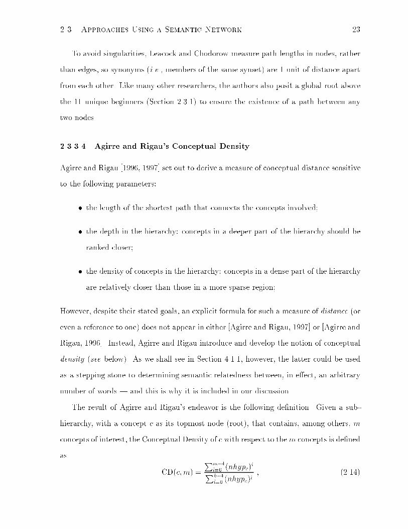
Figure 2.1: The quasi-geometric intuition behind Formula 2.14 for the case m < h. The
outer triangle marks the boundary of the subhierarchy rooted in c; the inner that of
the expected subhierarchy containing the m concepts of interest (depicted as solid-�lled
circles).
where nhypc is the mean number of hyponyms per node in c's subhierarchy (see below)
and h is the height of the subhierarchy.18
This formula can be given a quasi-geometric interpretation, as follows. If our sub-
hierarchy were a perfect nhypc-ary tree and the `area' of a hierarchy were taken to be
the number of concepts in it, then (see Figure 2.1) the denominator of the right-hand
side of Equation 2.14 would represent precisely the area of the subhierarchy rooted in c.
Similarly, the numerator would then represent the area of the largest minimal hierarchy
18Like Leacock and Chodorow (Section 2.3.3.3), Agirre and Rigau measure heights in nodes, so ahierarchy consisting of a single concept (e.g., c alone) is considered to have height h = 1.
2.3. Approaches Using a Semantic Network 25
required to accommodatem concepts (i.e., the (expected) case of each of the m concepts
occurring at a di�erent, but adjacent, (depth) level, thus resulting in a hierarchy of height
m). The fraction on the right-hand side of 2.14 would then express the ratio between
the areas of the expected-case hierarchy `covering' m concepts of interest and the actual
hierarchy in which they are found, hence justifying the term density in the name of the
measure. (Note, that if m > h, then also CD(c;m) > 1.)
In fact, our premise concerning a perfect nhypc-ary tree is not as unrealistic as it may
appear at �rst: the value of nhypc, in Agirre and Rigau's method, is computed for each
concept c in WordNet from the following equation:
descendantsc =h�1Xi=0
nhypic : (2.15)
Here, descendantsc is the number of concepts in the subhierarchy below c, including c
itself;19 thus the denominator of the right-hand side of Equation 2.14 does indeed express
the total number of concepts in c's subhierarchy.
Once the basic formula (Equation 2.14) had been established, the authors decided to
investigate possibilities of �ne-tuning it by introducing parameters � and � as follows:
CD(c;m) =
Pm�1i=0 (nhypc + �)i
�
descendantsc: (2.16)
After extensive experimentation with di�erent values of � and �, the authors concluded
that the latter does not a�ect the behavior of the formula, while the former does, yielding
the best results with � in the vicinity of 0.2. The �nal formula for Conceptual Density
is thus:
CD(c;m) =
Pm�1i=0 nhypi
0:2
c
descendantsc: (2.17)
19Agirre and Rigau are rather vague about the meaning of descendantsc, never explicitly de�ning it.They do, however, describe Equation 2.15 as capturing \the relation among height, averaged number ofhyponyms of each sense, and total number of senses in a subhierarchy" [Agirre and Rigau, 1997] andmention \the number of descendant senses of concept c" (ibid.) when talking about the denominator ofthe fraction in 2.14. Both of these remarks seem to corroborate our reading of the notation.
26 Chapter 2. Recent Approaches to Measuring Semantic Relatedness
2.4 Integrated Approaches
Like the methods in the preceding subsection, the �nal group of approaches that we
present in this report attempt to counter problems inherent in a general ontology. These
approaches incorporate an additional, and qualitatively di�erent, knowledge source: all
three techniques outlined below use corpus analysis to augment the information already
present in the network. As a side-e�ect, this \provides a way of adapting a static knowl-
edge structure to multiple contexts" [Resnik, 1995].
2.4.1 Resnik's Information-Based Approach
The key underlying idea of Resnik's [1995] approach is the intuition that one criterion
of similarity between two concepts is \the extent to which they share information in
common", which in an is-a taxonomy can be determined by inspecting the relative
position of a most speci�c concept that subsumes them both.20 This intuition seems to
be indirectly captured by edge-counting methods (such as that of Rada and colleagues
Section 2.3.2.1) in that \if the minimal path of is-a links between two nodes is long, that
means it is necessary to go high in the taxonomy, to more abstract concepts, in order to
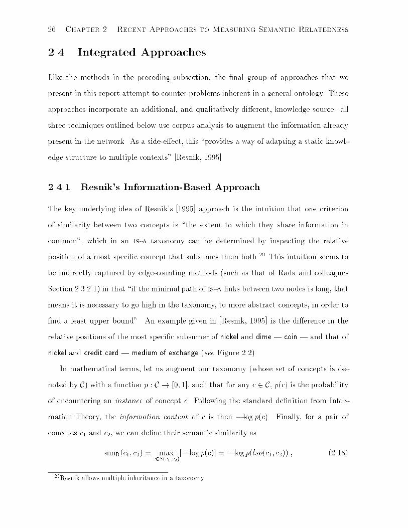
�nd a least upper bound". An example given in [Resnik, 1995] is the di�erence in the
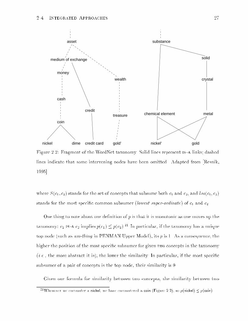
relative positions of the most speci�c subsumer of nickel and dime | coin | and that of
nickel and credit card | medium of exchange (see Figure 2.2).
In mathematical terms, let us augment our taxonomy (whose set of concepts is de-
noted by C) with a function p : C ! [0; 1], such that for any c 2 C, p(c) is the probability
of encountering an instance of concept c. Following the standard de�nition from Infor-
mation Theory, the information content of c is then � log p(c). Finally, for a pair of
concepts c1 and c2, we can de�ne their semantic similarity as
simR(c1; c2) = maxc2S(c1;c2)
[� log p(c)] = � log p(lso(c1; c2)) ; (2.18)
20Resnik allows multiple inheritance in a taxonomy.
2.4. Integrated Approaches 27
credit card
medium of exchange
credit
nickel’ gold
metal
crystal
solid
substance
chemical elementtreasure
wealth
gold’
asset
money
cash
coin
nickel dime
Figure 2.2: Fragment of the WordNet taxonomy. Solid lines represent is-a links; dashed
lines indicate that some intervening nodes have been omitted. Adapted from [Resnik,
1995].
where S(c1; c2) stands for the set of concepts that subsume both c1 and c2, and lso(c1; c2)
stands for the most speci�c common subsumer (lowest super-ordinate) of c1 and c2.
One thing to note about our de�nition of p is that it is monotonic as one moves up the
taxonomy: c1 is-a c2 implies p(c1) � p(c2).21 In particular, if the taxonomy has a unique
top node (such as um-thing in PENMAN Upper Model), its p is 1. As a consequence, the
higher the position of the most speci�c subsumer for given two concepts in the taxonomy
(i.e., the more abstract it is), the lower the similarity. In particular, if the most speci�c
subsumer of a pair of concepts is the top node, their similarity is 0.
Given our formula for similarity between two concepts, the similarity between two
21Whenever we encounter a nickel, we have encountered a coin (Figure 2.2), so p(nickel) � p(coin).
28 Chapter 2. Recent Approaches to Measuring Semantic Relatedness
words w1 and w2 can be calculated as
simR(w1; w2) = maxc12s(w1);c22s(w2)
[sim(c1; c2)] ; (2.19)
with s(wi) (i = 1; 2) as in Equation 2.13 (Section 2.3.3.3).
In Resnik's experiments, frequencies of concepts in the taxonomy were estimated
through noun frequencies gathered from the Brown Corpus of American English [Francis
and Ku�cera, 1982], a 1-million-word \collection of text across genres ranging from news
articles to science �ction". The key characteristic of his counting method is that an
individual occurrence of any noun in the corpus \was counted as an occurrence of each
taxonomic class containing it" (see below). For example, an occurrence of the noun nickel
was, in accordance with Figure 2.2, counted towards the frequency of nickel, coin, and so
forth. Note that, as a consequence of using raw (non-disambiguated) data, encountering
a word will contribute to the counts of all its senses (if it is polysemous) and those of
any of its homographs. So in case of nickel, the counts of nickel 0, chemical element, metal,
etc., will also be increased.
Formally,
freq(c) =X
n2words(c)
count(n) ; (2.20)
where words(c) is the set of words whose senses are subsumed by concept c (provided
that subsumption is re exive), and, adopting the maximum likelihood estimate (MLE)
rule,
p(c) =freq(c)
N; (2.21)
where N is the total number of nouns in the corpus which are also present in WordNet.
2.4.2 Jiang and Conrath's Combined Approach
Resnik's approach described above attempts to deal with the problem of \varying link
distances" [Resnik, 1995] (see Section 2.3.3) by generally downplaying the role of network
2.4. Integrated Approaches 29
edges in the determination of the degree of semantic proximity: edges are used solely for
locating super-ordinates of a pair of concepts; in particular, the number of links does not
�gure in any of the formulas pertaining to the method; numerical evidence comes from
corpus statistics, which are associated with nodes.
Such a selective use of the structure of the taxonomy, however, has its drawbacks, one
of which is the indistinguishability, in terms of semantic distance, of any two pairs of con-
cepts having the samemost-speci�c subsumer. Going back to Figure 2.2, simR(money; credit) =
simR(dime; credit card) = � log p(medium of exchange), whereas, for a typical edge-based
method such as Leacock and Chodorow's (Section 2.3.3.3), clearly simLC(money; credit) 6=
simLC(dime; credit card).
Jiang and Conrath's [1997] idea was to synthesize edge- and node-based techniques
(hence it is a combined approach) by e�ectively restoring the dominant function of net-
work edges in similarity computations and using corpus statistics as a corrective factor.
They hypothesized that the general formula for the weight of a link between a child-
concept cc and its parent-concept cp in a hierarchy should be of the form
wt(cc; cp) =
�� + (1� �)
�E
E(cp)
��d(cp) + 1
d(cp)
��
LS(cc; cp) T (cc; cp) ; (2.22)
where E(cp) denotes the number of children of cp (\local density"), �E denotes the average
local density over the entire hierarchy, d(cp) the depth of the node cp in the hierarchy,
LS(cc; cp) the strength of the link between cc and cp, T (cc; cp) the link-type coe�cient,
and the parameters � 2 [0;1) and � 2 [0; 1] control the degree of contribution of the
node depth and the density factor, respectively. A careful reader may notice a parallel
between the local density, node depth, and link-type factors in Equation 2.22 and type-
speci�c fanout, edge depth, and relation weight of Sussna's approach (Section 2.3.3.1).
The emphases of the two research programs, however, have been di�erent. Unlike Sussna,
Jiang and Conrath to date have experimented only with a single link-type, is-a (per-
sonal communication), which was assigned T of 1. Their investigation into the roles
of the density and depth components have demonstrated that \they are not the major
30 Chapter 2. Recent Approaches to Measuring Semantic Relatedness
determinants of the overall edge weight": setting � = 0:5 and � = 0:3 resulted in \a
small performance improvement" over the simplest case of � = 0 and � = 1 (i.e., giving
no consideration to density or depth). The main focus of Jiang and Conrath's e�ort has
thus been the link-strength factor, with Equation 2.22 reduced to the special case
wt(cc; cp) = LS(cc; cp) : (2.23)
In the framework of the is-a hierarchy, Jiang and Conrath postulated the strength
LS(cc; cp) of the link connecting a child-concept cc to its parent-concept cp to be propor-
tionate to the conditional probability p(ccjcp) of encountering an instance of cc given an
instance of cp. More speci�cally,
LS(cc; cp) = � log p(ccjcp) : (2.24)
By de�nition,
p(ccjcp) =p(cc&cp)
p(cp): (2.25)
If we adopt Resnik's scheme for assigning probabilities to concepts (Section 2.4.1), then
p(cc&cp) = p(cc), since any instance of a child is automatically an instance of its parent
(see footnote 21). Then,
p(ccjcp) =p(cc)
p(cp); (2.26)
and
LS(cc; cp) = IC(cc)� IC(cp) (2.27)
if we let IC(c) stand for the information content of concept c.
As per common practice, the semantic distance between an arbitrary pair of nodes
was taken to be the sum of the weights of the edges along the shortest path that connects
the nodes:
distJC(c1; c2) =X
c2path(c1;c2)rlso(c1;c2)
wt(c; par(c)) : (2.28)
Here, path(c1; c2) is the set of all the nodes in the shortest path from c1 to c2, and par(c)
returns the parent of the node c. One of the elements of path(c1; c2) in an is-a hierarchy
2.4. Integrated Approaches 31
will always be the most speci�c common subsumer of the two concepts, lso(c1; c2) (see
Section 2.4.1). Furthermore (and this explains its removal from path(c1; c2) in (2.28)), it
will be the only element without a parent in the same set.
Expanding the sum in the right-hand side of Equation 2.28, plugging in the expression
for the edge weight from Equation 2.23, and performing necessary eliminations will result
in the following �nal formulas for the semantic distance between concepts c1 and c2:
distJC(c1; c2) = IC(c1) + IC(c2) � 2 � IC(lso(c1; c2)) ; (2.29)
or
distJC(c1; c2) = 2 log p(lso(c1; c2)) � (log p(c1) + log p(c2)) : (2.30)
2.4.3 Lin's Universal Similarity Measure
Having noticed that all of the similarity measures known to him are tied to a particular
application, domain, or resource, Lin [1997a, 1997b, 1998] undertook an attempt to
de�ne a measure of similarity that is both universal (applicable to arbitrary objects
and \not presuming any form of knowledge representation") and theoretically justi�ed
(\derived from a set of assumptions" | instead of \directly by a formula" | so that \if
the assumptions are deemed reasonable, the similarity measure necessarily follows"). In
arriving at such a de�nition, he used the following three intuitions as a basis:
1. The similarity between A and B is related to their commonality.22 The more
commonality they share, the more similar they are.
2. The similarity between A and B is related to the di�erences between them. The
more di�erences they have, the less similar they are.
3. The maximumsimilarity betweenA and B is reached when A and B are identical,
no matter how much commonality they share.
22Throughout this subsection, A and B will denote arbitrary objects.
32 Chapter 2. Recent Approaches to Measuring Semantic Relatedness
Lin also found it necessary to introduce a few additional assumptions (and de�nitions),
notably that the commonality betweenA and B is measured by the amount of information
contained in \the proposition that states the commonalities" between them, formally
IC(common(A;B)) ; (2.31)
and that the di�erence between A and B is measured by
IC(description(A;B))� IC(common(A;B)) ; (2.32)
where description(A;B) is a proposition describing what A and B are.
Given the above setting and the apparatus of Information Theory, Lin was able to
prove the following
Similarity Theorem: The similarity between A and B is measured
by the ratio between the amount of information needed to state their
commonality and the information needed to fully describe what they are:
simL(A;B) =log P (common(A;B))
logP (description(A;B)): (2.33)
His measure of similarity between two concepts in a taxonomy ensued as a corollary:
simL(c1; c2) =2� log p(lso(c1; c2))
log p(c1) + log p(c2); (2.34)
where the notation is consistent with Equations 2.18 and 2.30. (The probabilities p(c)
are determined in a manner analogous to Resnik's pB(c) (Equation 2.21); refer to [Lin,
1997a] for details.)
As Lin points out, Resnik's similarity measure (Equation 2.18) is \quite close" to
simL. In fact, it can be shown that simR(c1; c2) =12IC(common(c1; c2)). What may be
a little more unexpected, Lin demonstrates that, under certain conditions, his similarity
measure coincides with Wu and Palmer's simWP(c1; c2) (Equation 2.11).
Chapter 3
Comparison with Human Judgement
3.1 Assessing Measures of Semantic Relatedness
How can we reason about computational measures of semantic relatedness? Given a
single measure, can we tell whether it is a good or a poor one? Given two measures, can
we tell whether one is better than the other?
Evaluation of semantic relatedness measures remains an open question [Agirre and
Rigau, 1997, Resnik, 1995, Hirst and St-Onge, 1998]. In our survey of literature on the
topic, we have come across three prevalent approaches: mathematical analysis, compar-
ison with human judgement, and application-speci�c evaluation.
The �rst approach (see, e.g., [Wei, 1993, Lin, 1998]) consists in a (chie y) theoretical
examination of mathematical properties of a measure, such as whether it is actually
a metric, whether it has singularities, whether its parameter-projections are smooth
functions, etc. Such analyses, in our opinion, may certainly aid the comparison of several
measures but perhaps not so much their individual assessment.
The second approach, comparison with human judgements of relatedness, does not
appear to su�er from the same limitations; in fact, it arguably yields the most generic as-
sessment of the `goodness' of a measure; however, its major drawback lies in the di�culty
33
34 Chapter 3. Comparison with Human Judgement
of obtaining such judgements (i.e., designing a psycholinguistic experiment, validating
its results, etc.). In his [1995] paper, Resnik presented a comparison of the ratings pro-
duced by his measure simR (and a couple of others) with those produced by human
subjects on a set of 30 word pairs (actually 28; see footnote 4, page 35) from an ex-
periment by Miller and Charles [1991]. The fact that others [Jiang and Conrath, 1997,
Lin, 1998] followed his lead and employed the same modestly sized dataset in their work
appears to be a testament to the seriousness of the problem.
Because of these de�ciencies, we, generally, have to take sides with the remaining
group of researchers who have chosen to evaluate their measures in the framework of a
particular NLP application (see Chapter 5).
However, since the trend has been established and since we have also found a use
for the results in our application-speci�c evaluation (Chapter 5), we decided to have the
measures implemented as part of the application-speci�c evaluation1 rate the Miller{
Charles pairs, as well as a superset thereof, and compare the ratings obtained with those
of human judges. The remainder of this chapter, then, discusses the outcome of our
e�ort.
3.2 The Data
The Miller{Charles word pairs mentioned above were actually derived from an earlier
study [Rubenstein and Goodenough, 1965]. As a part of an investigation into \the re-
lationship between similarity of context and similarity of meaning (synonymy)", Ruben-
stein and Goodenough obtained \synonymy judgements" by 51 human subjects on 65
pairs of words. The pairs ranged from \highly synonymous" to \semantically unrelated",
and the subjects were asked to rate them, on the scale of 0.0 to 4.0, according to their
\similarity of meaning" (see Table 3.1, columns 2 and 3). For the purposes of their study
1See Section 5.4.1 for the selection rationale and the implementation speci�cs.
3.3. The Results 35
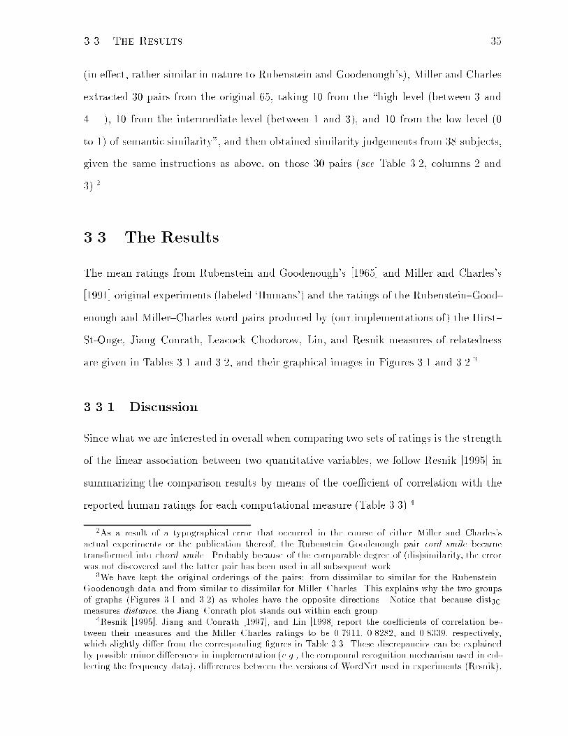
(in e�ect, rather similar in nature to Rubenstein and Goodenough's), Miller and Charles
extracted 30 pairs from the original 65, taking 10 from the \high level (between 3 and
4. . . ), 10 from the intermediate level (between 1 and 3), and 10 from the low level (0
to 1) of semantic similarity", and then obtained similarity judgements from 38 subjects,
given the same instructions as above, on those 30 pairs (see Table 3.2, columns 2 and
3).2
3.3 The Results
The mean ratings from Rubenstein and Goodenough's [1965] and Miller and Charles's
[1991] original experiments (labeled `Humans') and the ratings of the Rubenstein{Good-
enough and Miller{Charles word pairs produced by (our implementations of) the Hirst{
St-Onge, Jiang{Conrath, Leacock{Chodorow, Lin, and Resnik measures of relatedness
are given in Tables 3.1 and 3.2, and their graphical images in Figures 3.1 and 3.2.3
3.3.1 Discussion
Since what we are interested in overall when comparing two sets of ratings is the strength
of the linear association between two quantitative variables, we follow Resnik [1995] in
summarizing the comparison results by means of the coe�cient of correlation with the
reported human ratings for each computational measure (Table 3.3).4
2As a result of a typographical error that occurred in the course of either Miller and Charles'sactual experiments or the publication thereof, the Rubenstein{Goodenough pair cord{smile becametransformed into chord{smile. Probably because of the comparable degree of (dis)similarity, the errorwas not discovered and the latter pair has been used in all subsequent work.
3We have kept the original orderings of the pairs: from dissimilar to similar for the Rubenstein{Goodenough data and from similar to dissimilar for Miller{Charles. This explains why the two groupsof graphs (Figures 3.1 and 3.2) as wholes have the opposite directions. Notice that because distJCmeasures distance, the Jiang{Conrath plot stands out within each group.
4Resnik [1995], Jiang and Conrath [1997], and Lin [1998] report the coe�cients of correlation be-tween their measures and the Miller{Charles ratings to be 0.7911, 0.8282, and 0.8339, respectively,which slightly di�er from the corresponding �gures in Table 3.3. These discrepancies can be explainedby possible minor di�erences in implementation (e.g., the compound recognition mechanism used in col-lecting the frequency data), di�erences between the versions of WordNet used in experiments (Resnik),
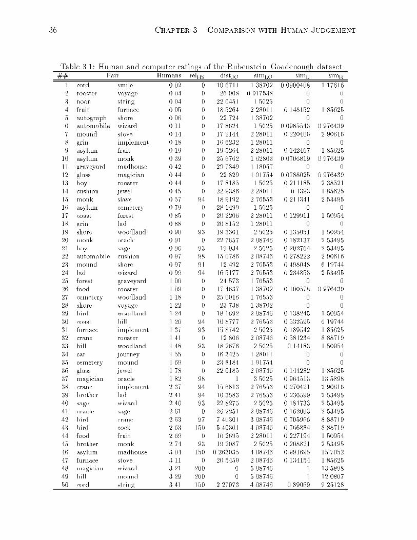
36 Chapter 3. Comparison with Human Judgement
Table 3.1: Human and computer ratings of the Rubenstein{Goodenough dataset.## Pair Humans relHS distJC simLC simL simR
1 cord smile 0.02 0 19.6711 1.38702 0.0900408 1.176162 rooster voyage 0.04 0 26.908 0.917538 0 03 noon string 0.04 0 22.6451 1.5025 0 04 fruit furnace 0.05 0 18.5264 2.28011 0.148152 1.856255 autograph shore 0.06 0 22.724 1.38702 0 06 automobile wizard 0.11 0 17.8624 1.5025 0.0985543 0.9764397 mound stove 0.14 0 17.2144 2.28011 0.220406 2.906168 grin implement 0.18 0 16.6232 1.28011 0 09 asylum fruit 0.19 0 19.5264 2.28011 0.142467 1.8562510 asylum monk 0.39 0 25.6762 1.62803 0.0706819 0.97643911 graveyard madhouse 0.42 0 29.7349 1.18057 0 012 glass magician 0.44 0 22.829 1.91754 0.0788025 0.97643913 boy rooster 0.44 0 17.8185 1.5025 0.211185 2.3852114 cushion jewel 0.45 0 22.9386 2.28011 0.1393 1.8562515 monk slave 0.57 94 18.9192 2.76553 0.211341 2.5349516 asylum cemetery 0.79 0 28.1499 1.5025 0 017 coast forest 0.85 0 20.2206 2.28011 0.129911 1.5095418 grin lad 0.88 0 20.8152 1.28011 0 019 shore woodland 0.90 93 19.3361 2.5025 0.135051 1.5095420 monk oracle 0.91 0 22.7657 2.08746 0.182137 2.5349521 boy sage 0.96 93 19.934 2.5025 0.202764 2.5349522 automobile cushion 0.97 98 15.0786 2.08746 0.278222 2.9061623 mound shore 0.97 91 12.492 2.76553 0.498048 6.1974424 lad wizard 0.99 94 16.5177 2.76553 0.234853 2.5349525 forest graveyard 1.00 0 24.573 1.76553 0 026 food rooster 1.09 0 17.4637 1.38702 0.100578 0.97643927 cemetery woodland 1.18 0 25.0016 1.76553 0 028 shore voyage 1.22 0 23.738 1.38702 0 029 bird woodland 1.24 0 18.1692 2.08746 0.138245 1.5095430 coast hill 1.26 94 10.8777 2.76553 0.532595 6.1974431 furnace implement 1.37 93 15.8742 2.5025 0.189542 1.8562532 crane rooster 1.41 0 12.806 2.08746 0.581234 8.8871933 hill woodland 1.48 93 18.2676 2.5025 0.14183 1.5095434 car journey 1.55 0 16.3425 1.28011 0 035 cemetery mound 1.69 0 23.8184 1.91754 0 036 glass jewel 1.78 0 22.0185 2.08746 0.144282 1.8562537 magician oracle 1.82 98 1 3.5025 0.964513 13.589838 crane implement 2.37 94 15.6813 2.76553 0.270421 2.9061639 brother lad 2.41 94 16.3583 2.76553 0.236599 2.5349540 sage wizard 2.46 93 22.8275 2.5025 0.181733 2.5349541 oracle sage 2.61 0 26.2251 2.08746 0.162003 2.5349542 bird crane 2.63 97 7.40301 3.08746 0.705966 8.8871943 bird cock 2.63 150 5.40301 4.08746 0.766884 8.8871944 food fruit 2.69 0 10.2695 2.28011 0.227194 1.5095445 brother monk 2.74 93 19.2087 2.5025 0.208821 2.5349546 asylum madhouse 3.04 150 0.263035 4.08746 0.991695 15.705247 furnace stove 3.11 0 20.5459 2.08746 0.134154 1.8562548 magician wizard 3.21 200 0 5.08746 1 13.589849 hill mound 3.29 200 0 5.08746 1 12.080750 cord string 3.41 150 2.27073 4.08746 0.89069 9.25128
3.3. The Results 37
Table 3.1: Human and computer ratings of the Rubenstein{Goodenough dataset (cont'd).## Pair Humans relHS distJC simLC simL simR
51 glass tumbler 3.45 150 5.94251 4.08746 0.792495 11.347752 grin smile 3.46 200 0 5.08746 1 10.419853 serf slave 3.46 0 19.8021 2.28011 0.34799 5.284454 journey voyage 3.58 150 5.21325 4.08746 0.747567 7.7193955 autograph signature 3.59 150 2.41504 4.08746 0.922084 14.290256 coast shore 3.60 150 0.884523 4.08746 0.96175 11.120357 forest woodland 3.65 200 0 5.08746 1 11.234958 implement tool 3.66 150 1.17766 4.08746 0.913309 6.203459 cock rooster 3.68 200 0 5.08746 1 14.290260 boy lad 3.82 150 5.39415 4.08746 0.728545 8.2986861 cushion pillow 3.84 150 0.70044 4.08746 0.974877 13.589862 cemetery graveyard 3.88 200 0 5.08746 1 13.766663 automobile car 3.92 200 0 5.08746 1 8.6230964 midday noon 3.94 200 0 5.08746 1 15.968365 gem jewel 3.94 200 0 5.08746 1 14.3833
Table 3.2: Human and computer ratings of the Miller{Charles dataset.## Pair Humans relHS distJC simLC simL simR
1 car automobile 3.92 200 0 5.08746 1 8.623092 gem jewel 3.84 200 0 5.08746 1 14.38333 journey voyage 3.84 150 5.21325 4.08746 0.747567 7.719394 boy lad 3.76 150 5.39415 4.08746 0.728545 8.298685 coast shore 3.70 150 0.884523 4.08746 0.96175 11.12036 asylum madhouse 3.61 150 0.263035 4.08746 0.991695 15.70527 magician wizard 3.50 200 0 5.08746 1 13.58988 midday noon 3.42 200 0 5.08746 1 15.96839 furnace stove 3.11 0 20.5459 2.08746 0.134154 1.8562510 food fruit 3.08 0 10.2695 2.28011 0.227194 1.5095411 bird cock 3.05 150 5.40301 4.08746 0.766884 8.8871912 bird crane 2.97 97 7.40301 3.08746 0.705966 8.8871913 tool implement 2.95 150 1.17766 4.08746 0.913309 6.203414 brother monk 2.82 93 19.2087 2.5025 0.208821 2.5349515 lad brother 1.66 94 16.3583 2.76553 0.236599 2.5349516 crane implement 1.68 94 15.6813 2.76553 0.270421 2.9061617 journey car 1.16 0 16.3425 1.28011 0 018 monk oracle 1.10 0 22.7657 2.08746 0.182137 2.5349519 cemetery woodland 0.95 0 25.0016 1.76553 0 020 food rooster 0.89 0 17.4637 1.38702 0.100578 0.97643921 coast hill 0.87 94 10.8777 2.76553 0.532595 6.1974422 forest graveyard 0.84 0 24.573 1.76553 0 023 shore woodland 0.63 93 19.3361 2.5025 0.135051 1.5095424 monk slave 0.55 94 18.9192 2.76553 0.211341 2.5349525 coast forest 0.42 0 20.2206 2.28011 0.129911 1.5095426 lad wizard 0.42 94 16.5177 2.76553 0.234853 2.5349527 chord smile 0.13 0 20.2418 1.62803 0.180828 2.2341328 glass magician 0.11 0 22.829 1.91754 0.0788025 0.97643929 rooster voyage 0.08 0 26.908 0.917538 0 030 noon string 0.08 0 22.6451 1.5025 0 0
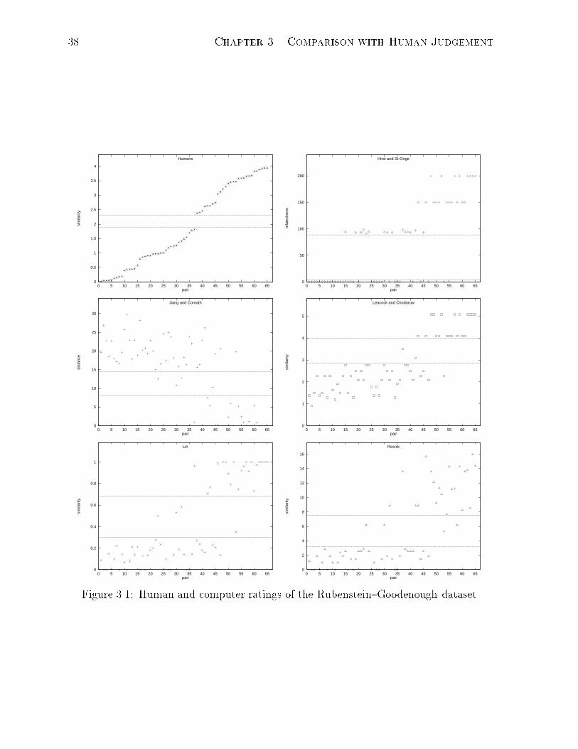
38 Chapter 3. Comparison with Human Judgement
0
0.5
1
1.5
2
2.5
3
3.5
4
0 5 10 15 20 25 30 35 40 45 50 55 60 65
sim
ilarit
y
pair
Humans
0
50
100
150
200
0 5 10 15 20 25 30 35 40 45 50 55 60 65re
late
dnes
spair
Hirst and St-Onge
0
5
10
15
20
25
30
0 5 10 15 20 25 30 35 40 45 50 55 60 65
dist
ance
pair
Jiang and Conrath
0
1
2
3
4
5
0 5 10 15 20 25 30 35 40 45 50 55 60 65
sim
ilarit
y
pair
Leacock and Chodorow
0
0.2
0.4
0.6
0.8
1
0 5 10 15 20 25 30 35 40 45 50 55 60 65
sim
ilarit
y
pair
Lin
0
2
4
6
8
10
12
14
16
0 5 10 15 20 25 30 35 40 45 50 55 60 65
sim
ilarit
y
pair
Resnik
Figure 3.1: Human and computer ratings of the Rubenstein{Goodenough dataset.
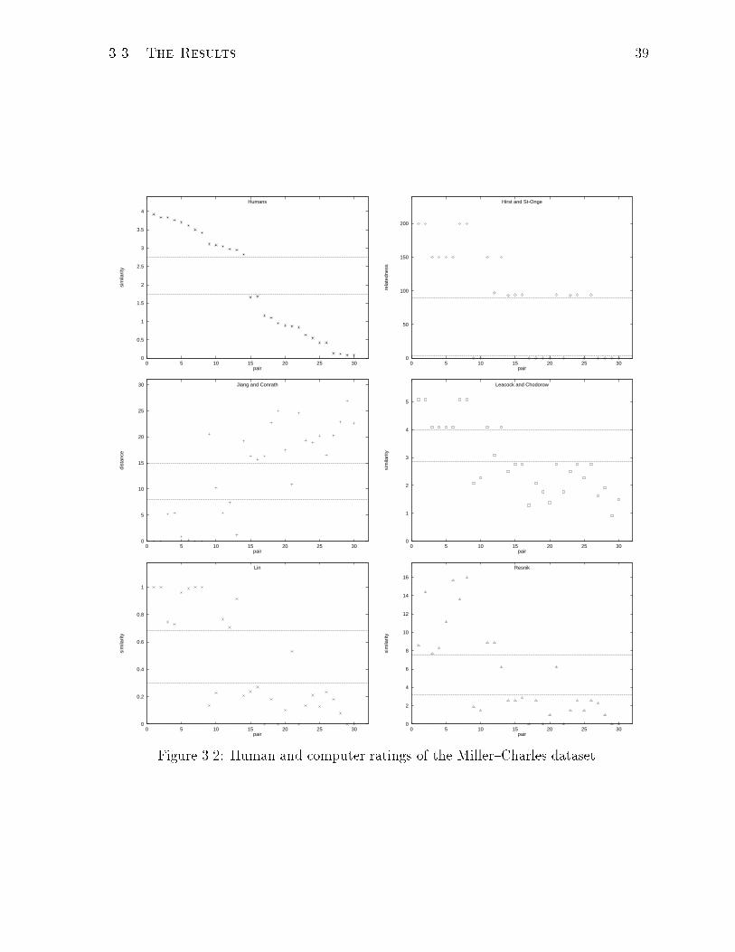
3.3. The Results 39
0
0.5
1
1.5
2
2.5
3
3.5
4
0 5 10 15 20 25 30
sim
ilarit
y
pair
Humans
0
50
100
150
200
0 5 10 15 20 25 30
rela
tedn
ess
pair
Hirst and St-Onge
0
5
10
15
20
25
30
0 5 10 15 20 25 30
dist
ance
pair
Jiang and Conrath
0
1
2
3
4
5
0 5 10 15 20 25 30
sim
ilarit
y
pair
Leacock and Chodorow
0
0.2
0.4
0.6
0.8
1
0 5 10 15 20 25 30
sim
ilarit
y
pair
Lin
0
2
4
6
8
10
12
14
16
0 5 10 15 20 25 30
sim
ilarit
y
pair
Resnik
Figure 3.2: Human and computer ratings of the Miller{Charles dataset.
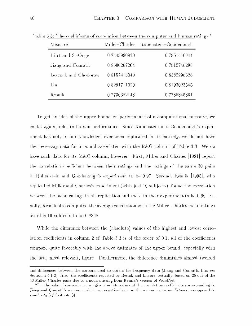
40 Chapter 3. Comparison with Human Judgement
Table 3.3: The coe�cients of correlation between the computer and human ratings.5
Measure Miller{Charles Rubenstein{Goodenough
Hirst and St-Onge 0.7443990930 0.7861440344
Jiang and Conrath 0.8500267204 0.7812746298
Leacock and Chodorow 0.8157413049 0.8382296528
Lin 0.8291711020 0.8193023545
Resnik 0.7736382148 0.7786845861
To get an idea of the upper bound on performance of a computational measure, we
could, again, refer to human performance. Since Rubenstein and Goodenough's exper-
iment has not, to our knowledge, ever been replicated in its entirety, we do not have
the necessary data for a bound associated with the R&G column of Table 3.3. We do
have such data for its M&C column, however. First, Miller and Charles [1991] report
the correlation coe�cient between their ratings and the ratings of the same 30 pairs
in Rubenstein and Goodenough's experiment to be 0.97. Second, Resnik [1995], who
replicated Miller and Charles's experiment (with just 10 subjects), found the correlation
between the mean ratings in his replication and those in their experiment to be 0.96. Fi-
nally, Resnik also computed the average correlation with the Miller{Charles mean ratings
over his 10 subjects to be 0.8848.
While the di�erence between the (absolute) values of the highest and lowest corre-
lation coe�cients in column 2 of Table 3.3 is of the order of 0.1, all of the coe�cients
compare quite favorably with the above estimates of the upper bound, especially with
the last, most relevant, �gure. Furthermore, the di�erence diminishes almost twofold
and di�erences between the corpora used to obtain the frequency data (Jiang and Conrath, Lin; seeSection 5.4.1.2). Also, the coe�cients reported by Resnik and Lin are, actually, based on 28 out of the30 Miller{Charles pairs due to a noun missing from Resnik's version of WordNet.
5For the sake of convenience, we give absolute values of the correlation coe�cients corresponding toJiang and Conrath's measure, which are negative because the measure returns distance, as opposed tosimilarity (cf footnote 3).
3.3. The Results 41
as we consider the larger Rubenstein{Goodenough dataset. In fact, the measures are
divided in their reaction to increasing the size of the dataset: the correlation improves
for relHS, simLC, and simR but deteriorates for distJC and simL. This division might not
be arbitrary: the last two depend on the same three quantities, log p(c1), log p(c2), and
log p(lso(c1; c2)) (see Equations 2.30 and 2.34).6 However, with the present amount of
evidence, this connection remains hypothetical.
An examination of the graphs in Figures 3.1 and 3.2 gives rise to several more
points. Of the �ve computational measures, the discrete nature of the Hirst{St-Onge
and Leacock{Chodorow measures is much more apparent from the graphs than that of
the others: i.e., a �xed number of levels encompassing a non-trivial number of points can
be rather easily distinguished in the plots of the ratings produced by relHS and simLC.
This, of course, is a result of their being based on the same highly discrete factor: the
path length.
As a matter of fact, a more substantial correspondence between the two measures can
be recognized from the graphs and explained in the same way. In each dataset, the upper
portions of the Hirst{St-Onge (relHS � 150) and Leacock{Chodorow (simLC > 4) graphs
look the same: namely, the sets of pairs a�ording the highest and the second highest
values of the two measures are identical. This happens because the sets are composed of
synonym and parent-child pairs, respectively.7
Further down the Y -axis, we �nd that the two graphs still mirror each other quite
closely in the middle region (2.4{3.2 for simLC and 90{100 for relHS) for the Miller{
Charles data. For the larger set of Rubenstein and Goodenough's, however, di�erences
begin to surface. The pair automobile{cushion (22), for instance, is ranked even with
magician{oracle (37) by the Hirst{St-Onge measure but far below both magician{oracle
6In fact, the coe�cient for simR, which depends on one of the three, log p(lso(c1; c2)), improves onlyin the third digit.
7 In general, the inverse image of the second highest value for simLC is a proper subset of that forrelHS, for the latter would also include all the antonym and meronym-holonym pairs. The two datasetsat hand, however, do not seem to contain any examples from these categories.
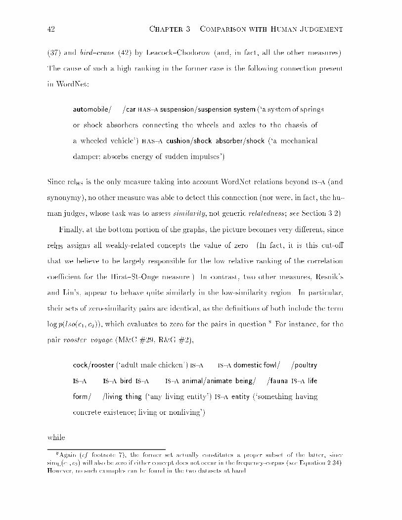
42 Chapter 3. Comparison with Human Judgement
(37) and bird{crane (42) by Leacock{Chodorow (and, in fact, all the other measures).
The cause of such a high ranking in the former case is the following connection present
in WordNet:
automobile/. . . /car has-a suspension/suspension system (`a system of springs
or shock absorbers connecting the wheels and axles to the chassis of
a wheeled vehicle') has-a cushion/shock absorber/shock (`a mechanical
damper; absorbs energy of sudden impulses').
Since relHS is the only measure taking into account WordNet relations beyond is-a (and
synonymy), no other measure was able to detect this connection (nor were, in fact, the hu-
man judges, whose task was to assess similarity, not generic relatedness; see Section 3.2).
Finally, at the bottom portion of the graphs, the picture becomes very di�erent, since
relHS assigns all weakly-related concepts the value of zero. (In fact, it is this cut-o�
that we believe to be largely responsible for the low relative ranking of the correlation
coe�cient for the Hirst{St-Onge measure.) In contrast, two other measures, Resnik's
and Lin's, appear to behave quite similarly in the low-similarity region. In particular,
their sets of zero-similarity pairs are identical, as the de�nitions of both include the term
log p(lso(c1; c2)), which evaluates to zero for the pairs in question.8 For instance, for the
pair rooster{voyage (M&C #29, R&G #2),
cock/rooster (`adult male chicken') is-a . . . is-a domestic fowl/. . . /poultry
is-a . . . is-a bird is-a . . . is-a animal/animate being/. . . /fauna is-a life
form/. . . /living thing (`any living entity') is-a entity (`something having
concrete existence; living or nonliving')
while
8Again (cf footnote 7), the former set actually constitutes a proper subset of the latter, sincesimL(c1; c2) will also be zero if either concept does not occur in the frequency-corpus (see Equation 2.34).However, no such examples can be found in the two datasets at hand.
3.3. The Results 43
voyage is-a journey/journeying is-a travel/. . . /traveling is-a change of loca-
tion/. . . /motion is-a change (`the act of changing something') is-a action
(`something done (usually as opposed to something said)') is-a act/human
action/human activity (`something that people do or cause to happen').
Entity and act are both `unique beginners' (see Section 2.3.1); hence the sole common
subsumer of rooster and voyage (and hence their lso) is the (fake) global root (see Sec-
tion 2.3.3.3), which, in turn, is the only concept whose p is 1. Analogously, although,
perhaps, somewhat more surprisingly for a human reader, for the pair asylum{cemetery
(R&G #16), simL = simR = 0, since
asylum/insane asylum/. . . /mental hospital is-a hospital/in�rmary is-a med-
ical building (`a building where medicine is practiced') is-a building/edi�ce
is-a . . . is-a artifact/artefact (`a man-made object') is-a object/inanimate
object/physical object (`a nonliving entity') is-a entity
whereas
cemetery/graveyard/. . . /necropolis (`a tract of land used for burials') is-a
site (`the piece of land on which something is located (or is to be located)')
is-a position/place (`the particular portion of space occupied by a physical
object') is-a . . . is-a location (`a point or extent in space').
Looking back at the high-similarity portion of the graphs, but now taking into con-
sideration the rest of the measures, we can make a couple more observations. First,
the graphs of all of the measures exhibit a `line' of synonyms (comprising four points
for the Miller{Charles dataset and nine points for Rubenstein{Goodenough) at the top
(bottom for Jiang and Conrath's measure), except for Resnik's. In the latter case,
simR(c; c) = � log p(lso(c; c)) = � log p(c) (see Equation 2.18); hence the similarity be-
tween a concept and itself may vary from one concept to another. Second, the afore-
mentioned `lines' are not continuous, as one might expect from the graphs of the human
44 Chapter 3. Comparison with Human Judgement
judgements: for the Miller{Charles set, for instance, the line includes pairs 1, 2, 7, and 8,
while missing pairs 3{6. This peculiarity is due entirely to WordNet, according to which
gem and jewel (pair 2) are synonyms, whereas journey and voyage (pair 3), boy and lad
(pair 4), and even asylum and madhouse (pair 6) are not:
lad/laddie/cub/sonny/sonny boy (`a male child (a familiar term of address
to a boy)') is-a boy/male child/child (`a young male person'),
voyage (`a journey to some distant place') is-a journey/journeying (`the
act of traveling from one place to another'),
madhouse/nuthouse/. . . /sanatorium (`pejorative terms for an insane asy-
lum') is-a asylum/insane asylum/. . . /mental hospital (`a hospital for men-
tally incompetent or unbalanced persons').
| while magician and wizard (pair 7) are synonyms again.
Although, as we saw above, already for two measures the details of their medium-
similarity regions di�er, there appears to be an interesting commonality at the level of
general structure: in the vicinity of sim = 2, the plots of human similarity ratings for both
the Miller{Charles and the Rubenstein{Goodenough dataset display an easily discernible
horizontal band that contains no points. For the Miller{Charles data (Figure 3.2), the
band separates the pair crane{implement (16) from brother{monk (14),9 and for the
Rubenstein{Goodenough (Figure 3.1), it separates magician{oracle (37) from crane{
implement (38). On the graphs of computed ratings, to these void strips we can put
in correspondence regions with at most a few points (up to 2 for the Miller{Charles set
and up to 4 for the Rubenstein{Goodenough set). As we will argue in Section 5.4.2, this
commonality may bear more signi�cance than at �rst appears, as it suggests that, if we
9Miller and Charles ordered their pairs according to the opinions of their subjects, except, for somereason, the pairs lad{brother (15) and crane{implement (16), whose ratings were 1.66 and 1.68, re-spectively, according to their subjects but 2.41 and 2.37, respectively, according to Rubenstein andGoodenough's subjects.

3.3. The Results 45
were to partition the set of all pairs into the related and the unrelated, the boundary
between the two subsets, for each measure (and for the human judgements, for that
matter), should lie somewhere within these regions.

46 Chapter 3. Comparison with Human Judgement
Chapter 4
Some Applications and Relevant
Results
As we argued in Section 1.1, the continuing interest in measuring semantic relatedness
can be probably best explained by its wide applicability. Furthermore, for the reasons
outlined in Section 3.1, the majority of researchers whose work was presented in Chap-
ter 2, have chosen to test their approaches in the framework of a particular application,
thereby either rendering them comparable with others or at least allowing for some
performance-related intuition. In this chapter, then, we discuss, in varying degrees of
detail, some applications of the methods reviewed earlier as well as the relevant results
that experimentation with them has produced.
4.1 Resolution of Word Sense Ambiguity
The task of resolving word sense, or lexical, ambiguity | also known as word sense
disambiguation (WSD) or word sense identi�cation | can be viewed as establishment
of a correspondence between a use of a word in a text and its appropriate sense in a
lexicon. A great many words, in any natural language, have more than one meaning,
owing to polysemy, homonymy/homography, and categorial ambiguity [Hirst, 1987], with
47
48 Chapter 4. Some Applications and Relevant Results
some English words' senses numbering in excess of 60 (e.g., the verb go) [Amsler, 1980].
As Leacock and Chodorow [1998] point out, \some level of word sense identi�cation
is required for virtually all natural language processing applications". The approaches
presented below all attempt to tackle this fundamental task, with the help of a measure
of semantic relatedness.
4.1.1 Agirre and Rigau
In Agirre and Rigau's method, \given a window size, the program moves the window one
noun at a time from the beginning of the document towards its end, disambiguating in
each step the noun in the middle of the window and considering the other nouns in the
window as context" [Agirre and Rigau, 1996]. For each particular window W with the
middle word w, the program computes the Conceptual Density of every nominal concept
in WordNet with respect to the senses of the words in W that the concept contains in its
subhierarchy (see Section 2.3.3.4). \It selects the concept c with the highest Conceptual
Density and selects the senses below it as the correct senses for the respective words"1
| the rest of their senses are then eliminated from further consideration. Unfortunately,
both [Agirre and Rigau, 1996] and [Agirre and Rigau, 1997] seem a little unclear as to
what exactly happens next, but we can imagine the following scenario. If, as a result
of the above process, w is down to a single sense, we are done, and the window can
advance. Otherwise, we can repeat the process with the remaining senses of the words
in W : since there are fewer of them now, the conceptual density values should change
(Equation 2.17). If, however, no senses (of any words in W ) were eliminated during the
1This is the place in Agirre and Rigau's method to which we referred in Section 2.3.3.4 when claim-ing that their Conceptual Density (2.17) could be used to derive a measure of semantic relatedness.According to the description above, one obvious way to do this is to de�ne
relAR(w1; : : : ; wm) = maxc2L
CD(c;m) ;
where w1; : : : ; wm are the contents of W (including w) and L is the entire lexicon (in this case, the nounpart of WordNet).
4.1. Resolution of Word Sense Ambiguity 49
last iteration, then any further attempts to disambiguate w (with the current window)
are futile, and the word is considered genuinely ambiguous.
Agirre and Rigau [1997] describe an experiment that deployed this algorithm to dis-
ambiguate the noun portion of a 2079-word-long text randomly chosen from SemCor
[Miller et al., 1993] (a sense-tagged subset of the Brown Corpus). Out of the total of
564 nouns in the text, 464 were found in WordNet, of which 315 were polysemous. The
sense tags assigned by the algorithm were compared against the original sense tags con-
tained in SemCor in terms of precision, recall, and coverage.2 The overall performance
was found to be best for the window size of 25, yielding 88.6%, 66.4%, and 58.8% for
coverage, precision, and recall, respectively, and 83.2%, 47.3%, and 39.4% if polysemous
nouns only were considered.
The algorithm was found to considerably outperform (on the order of 15%) the `guess-
ing baseline' (selecting senses at random) in precision and give a 10% better coverage
than the `most frequent' heuristic3 (the precision in this case was about the same).
In a followup study, reported by Agirre and Rigau [1996], four SemCor texts were
used, containing the total of 1858 WordNet nouns, of which 1256 were polysemous. The
overall coverage, precision, and recall came out between 2% and 5% lower, and the
optimal context (window) size was found to vary depending on the genre of the text.
All in all, Agirre and Rigau quali�ed the results as promising, \considering the di�-
culty of the task (free running text, large number of senses per word in WordNet), and
the lack of any discourse structure of the text".
2 Precision was computed as the ratio of the number of correctly disambiguated nouns to the totalnumber of disambiguated nouns, recall as the ratio of the number of correctly disambiguated nouns tothe total number of nouns considered, and coverage as the ratio of the total number of disambiguatednouns to the total number of nouns considered.
3The frequency counts for each sense were collected from the rest of SemCor.
50 Chapter 4. Some Applications and Relevant Results
4.1.2 Sussna
In Sussna's [1993] experiments, for a given window of words (terms) T = ft1; t2; : : : ; tng,
\each combination of n senses across the terms is tried, with one sense chosen at a time
for each term". For each such combination, the n(n�1)2
pairwise distances are summed to
arrive at an overall value, H(T ). If we let S denote the set of all sense combinations of
the terms in T , and S 2 S be a particular such combination (i.e., S = fs1; s2; : : : ; sng,
where each si is a sense of ti), then \the winning combination" is the S 2 S that produces
\the minimal `energy' "
Hmin(T ) = minS
Xx;y2S
distS(x; y) : (4.1)
How exactly the minimal-energy sense combination is used for disambiguation de-
pends on the variety of window, of which Sussna distinguishes several. For an initial
mutual constraint window, \all of the terms in the window are assigned . . . senses at the
same time." When working with a moving mutual constraint window, only the middle
term in the window is assigned its sense on the basis of Hmin. \Record is kept of the
winning sense, but when that term plays a role other than `middle term', its senses are
allowed to fully vary", thus giving a middle term \full bene�t of both previous and sub-
sequent context. All senses of surrounding terms are considered, not just their winning
senses." In frozen past approach, only the last term in the window is assigned its sense.
This strategy results in essentially linear-time processing, as \there are only as many
`combinations' to try as there are senses of the single term being disambiguated." Fi-
nally, various ways of combining these approaches are possible (e.g., a small set of initial
terms is processed with mutual constraint, and later terms are then processed with a
moving frozen-past window).
In the main evaluation, �ve documents from the Time magazine article collection
were considered, and the output of the \semantic distance software" was compared with
4.1. Resolution of Word Sense Ambiguity 51
that of \chance software"4 and human disambiguators.5 The comparison was conducted
by means of a couple of non-standard metrics invented by Sussna himself. His method's
performance fell almost exactly in the middle between the performance of the chance
software and that of human disambiguators.
An interesting fact, however, is that Agirre and Rigau, having noticed a certain degree
of similarity between their ideas and Sussna's, replicated his experiment and found their
precision (see footnote 2 on page 49) to be 60.1% against his 52.3% [Agirre and Rigau,
1996].
4.1.3 Leacock and Chodorow
Leacock and Chodorow [1998] conducted a \preliminary" investigation into using Word-
Net-based similarity as an aid to a statistical local-context classi�er.
A typical methodology is to train a classi�er on contexts that contain a polysemous
word of interest in a known sense. As Leacock and Chodorow point out, a fundamental
problem with this approach is the sparseness of training data: since they have to be
hand-disambiguated, \the task of collecting large training sets for each sense of each
polysemous word is simply not feasible". Leacock and Chodorow's idea is then to use
similarity to \�ll in gaps in a sparse training space", relying on the conjecture that
\semantically similar words should provide similar contextual clues". For example, if
baseball proves to be a good discriminator for a particular sense of the verb play, then
so should be words semantically similar to it, such as hockey, football, or soccer, even if
they are not initially a part of the training space.
Leacock and Chodorow tackled the problem of discerning among four senses of the
verb serve (`serve a function or purpose', `provide a service', `supply with food or drink',
4This is the same as the `guessing baseline' in Agirre and Rigau's experiments (Section 4.1.1).5The human disambiguators were given roughly the same information as the semantic distance soft-
ware: the list of nouns from the documents, with each noun accompanied by its synsets, their hypernymsynsets, and a gloss if available.
52 Chapter 4. Some Applications and Relevant Results
and `hold an o�ce') in all of their experiments. Sentence-length contexts for the verb and
its morphological variations were collected from the 25-million-word APHB corpus and
the 1987 edition of Wall Street Journal of a comparable size. This resulted in a corpus
containing at least 350 sentences for each of the four senses of serve,6 which were used
for building both training and testing sets for the experiments.
Leacock and Chodorow's original classi�er analyzed the local context in terms of its
part-of-speech, open-class-item, and closed-class-item composition. During the training
phase, three frequency distributions were derived. Given a verb-occurrence vi of serve
in a test set, a score, based on the likelihood of vi's local context according to these
distributions, was computed for each of the four possible senses of vi. The sense with the
highest score was then selected.
For the purposes of evaluation, senses returned by the classi�er were compared with
those assigned by human judges. With the optimal window size of �2, �6, and �2
positions7 for part-of-speech, open-class-item, and closed-class-item information, respec-
tively, the average performance, in terms of correctly identi�ed senses, was 75% for
training sets of size 50, 79% for training sets of size 100, and 83% for training sets of size
200.
Before adding a semantic component to their classi�er, Leacock and Chodorow de-
cided to experiment with similarity as a sole means of word sense identi�cation. They
formed \separate left and right context sets, corresponding very roughly to the subject
and complement of serve", by extracting the noun immediately preceding and the noun
immediately following each verbal instance of serve in the training set (and accounting for
passivization as necessary). Two semantic similarity measures, Leacock and Chodorow's
(Section 2.3.3.3) and Resnik's (Section 2.4.1), were run on the training and testing con-
6Each occurrence of the verb serve was tagged with a WordNet sense by two people, and only thesentences on which both taggers agreed were included in the �nal corpus.
7All sentences in Leacock and Chodorow's experiments were preprocessed with Brill's [1994] part-of-speech tagger. A position can then be de�ned as any syntactic unit awarded a separate tag (these wouldinclude compound nouns and punctuation).
4.1. Resolution of Word Sense Ambiguity 53
text sets. Since, as preliminary studies indicated, the complement of a verb appears to
have a higher predictive value than the subject, the right context was weighted over the
left context, resulting in the following algorithm:
1. the maximum similarity values between the right-context noun and the nouns in
all four right-context training sets were computed, and the sense with the highest
value was selected;
2. if a single sense could not be selected because of a tie or if the test occurrence
simply had no right context, the maximum similarity values were computed in an
analogous manner for the left context and the sense with the highest value was
chosen;
3. if two or more senses were tied for the �rst place or there was no left context,
don't know would be returned.
The algorithm was tested with the training set sizes of 10, 25, 50, 100, and 200. For
all of these, both similarity measures performed better than chance (the lowest average
percentage correct, delivered by Resnik's measure with training sets of 10 sentences,
being 35% versus 25% for chance). Comparatively, Leacock and Chodorow's measure
outperformed Resnik's for smaller training sets in terms of percentage correct (2{5%
di�erence), but the latter had fewer errors (0{8% di�erence). For 200-sentence training
sets, Resnik's measure fared slightly better than Leacock and Chodorow's. Overall,
however, the percentage of incorrect sense-assignments was rather high (up to 36% for
Leacock and Chodorow's trained on 10 sentences). In order to rectify that, Leacock
and Chodorow tried running the system with both measures at once, choosing a sense
only if it had the highest ranking according to both. This brought down the error rate
considerably (10{15%) but did so at the expense of recall (the percentage of don't
knows increased by 20{27%).
54 Chapter 4. Some Applications and Relevant Results
As a test of the generalizing power of similarity, Leacock and Chodorow conducted
another experiment, in which they compared the performance of a sense-identi�cation
algorithm based on exact base-form matches (which were found highly reliable by a num-
ber of researchers) with that of an algorithm combining exact matches with similarity-
matches. According to the �rst algorithm (which we will call EM ), a sense was selected
only if a test occurrence of serve had exactly the same noun to its right or to its left (in
this order of precedence) as an occurrence in the training set. In the second algorithm
(we will refer to it as EM+), after a context had been examined for an exact match
and none found, the similarity measures were consulted, and, if they agreed on the same
sense, that sense was chosen.8
The �rst algorithm achieved its best performance when trained on 200 sentences, cor-
rectly identifying, on average, 47% of the test occurrences and returning don't know
for 42%. The best performance of the second algorithm was 56% correct and 30% don't
know (for the same training set size). In general, \the exact-match-plus-semantic-
similarity approach more than doubled the e�ective size of the training set". That is,
the second algorithm consistently performed better than the �rst algorithm with twice
the training data. For instance, the second algorithm correctly identi�ed 54% of the test
occurrences of serve when trained on only 100 sentences, thereby surpassing the �rst
algorithm's 47% resulting from training on 200 sentences (see above). Similarly, while
the �rst algorithm achieved the accuracy of 39% after training on 50-sentence sets, the
second algorithm scored 43% with half of the training.
As an example of the similarity-induced \expansion" of the training space, nouns such
as tart, refrigerator, and caviar, occurring in test contexts but not in the training sets,
were found similar to the training context associated with the sense `supply with food or
drink' of the verb serve by both similarity measures, and hence the sense was correctly
8Compared with the algorithm described on the previous page, EM+ has the bene�t of consideringwords that are not in WordNet during its exact-match phase.
4.1. Resolution of Word Sense Ambiguity 55
determined by the second algorithm.
Since 56% was still a long way from 83%, Leacock and Chodorow concluded that
even the exact-match coupled with semantic similarity is not adequate as a stand-alone
classi�er9 and proceeded to combine the similarity-matching with their statistical local-
context classi�er. This was done in a fashion similar to the EM+ algorithm: the open-
class component of a given test context was compared with the training data; if a similar
(according to both measures) context was found, it was substituted for the training
context, and the revised sentence was then submitted to the statistical module of the
classi�er. For example, the words sauerbraten and dumpling were found to be similar
to dinner and bacon, respectively (both from the training corpus), so the test sentence
Sauerbraten is usually served with dumplings was replaced with Dinner is usually served
with bacon by the similarity-module.
Augmenting the statistical local-context classi�er with a similarity component re-
sulted in \a small but consistent improvement in the classi�er's performance". For train-
ing sets of size 200, the di�erence in the percentage correct was 0.6% (83.1% vs 82.5%),
but it increased as the training set size decreased, reaching 3.5% for 10 sentences (59.4%
vs 55.9%). The results should therefore be considered satisfactory, since, as Leacock and
Chodorow argue, it is precisely small training sets that are practical when it comes to
the task of collecting training data for a large number of words.
4.1.4 Lin
Lin also used his measure (2.34) in research on using local context for word sense disam-
biguation [Lin, 1997b].
In contrast with the common motto that \two occurrences of the same word have
identical meanings if they have similar local contexts", the intuition behind Lin's method
9\This is hardly suprising," they write, \as the local context needed for disambiguating verbs includesmore than just [their] arguments."
56 Chapter 4. Some Applications and Relevant Results
is that \two di�erent words are likely to have similar meanings if they occur in identical
local contexts".
The general idea of the method is �rst to compile a database of local contexts (de�ned
in terms of intrasentential syntactic dependencies; see [Lin, 1997b] for details); given that,
for each ambiguous word w we can extract selectors (the words occurring in identical
context in the database) and then, with the aid of the semantic distance function, choose
the sense of w that maximizes the similarity between the word and its selectors.10
Interestingly enough, Lin also used his similaritymeasure in performance evaluation of
the above disambiguation method. Cued by the observation that given \a list of senses in
a general-purpose lexical resource, even humans may frequently disagree with one another
on what the correct sense should be", he relaxed the criterion of correctness, counting
sanswer as correct as long as it is \similar enough" to the sense tag skey in SemCor. The
most relaxed interpretation of \similar enough" was taken to be simL(sanswer; skey) > 0
| which is true as long as sanswer and skey have a common subsumer in WordNet (e.g.,
they are both locations, living things, etc.). Naturally, the strictest interpretation is
simL(sanswer; skey) = 1, which is only true if sanswer and skey are identical. The compro-
mise between the two that Lin came up with was simL(sanswer; skey) > 0:23, where the
right-hand side is \the average similarity of 50,000 randomly generated pairs (w;w0) in
which w and w0 belong to the same Roget's category".
Lin used a 25-million-word Wall Street Journal corpus to construct his local context
database and the `press reportage' part of SemCor (about 14,000 words with 2,832 distinct
polysemous nouns) as a test set. Compared with the baseline strategy of always choosing
the WordNet-sense most frequent in SemCor, his method scored 56.1% vs baseline 58.9%
for the strictest criterion of correctness, 68.5% vs 64.2% for the intermediate one, and
73.6% vs 67.2% for the most relaxed criterion. Hence, whereas the algorithm actually
does a little worse than the baseline when it comes to choosing the right sense, once the
10The exact methodology of the last step falls outside of the scope of this report.
4.1. Resolution of Word Sense Ambiguity 57
correctness criteria are relaxed, its \performance gain" is considerably larger than that
of the baseline method. In other words, when the algorithm does make mistakes, \the
mistakes tend to be closer to the correct answer" than the most frequent sense is.
4.1.5 Okumura and Honda
Resolution of word sense ambiguity is also one of the applications investigated by Oku-
mura and Honda [1994]. In their framework, lexical disambiguation of a word consists in
deciding on its most likely thesaural category number. Since (recall from Section 2.2.3)
two words can enter into the same chain if and only if they belong to the same category
of Bunrui-goihyo, a word's sense is uniquely determined by the lexical chain the word is
added to.
In order for lexical chains \to function truly as local context", Okumura and Honda
arrange them in the order of salience that is based on the chain's recency and length:
longer and more recently updated chains are considered to better represent the topic in
the neighborhood. The key steps of the resulting algorithm are as follows:
1. select candidate words (nouns, verbs, and adjectives (with some exceptions));
2. check for intra-sentential lexical cohesion, i.e., attempt to build new chains out
of the candidate words within a sentence;
3. try to �t the remaining candidate words into existing lexical chains in order of
salience (which is updated along the way).
For the purposes of evaluation, the system was run on �ve texts taken from Japanese
language examination questions. The performance was calculated as the quotient of the
number of correctly disambiguated words by the number of ambiguous (but correctly
segmented) words. The system's average performance of 63.4% is considered promising
by Okumura and Honda, for they acknowledge the relative na��vet�e of their method (in
58 Chapter 4. Some Applications and Relevant Results
both the salience determination mechanism and the knowledge sources employed) and
they see immediate ways of improving it (for instance, by making use of the Japanese
topical marker `wa', etc.).
4.2 Identifying the Discourse Structure
4.2.1 Okumura and Honda
The second application of Okumura and Honda's lexical chains is based on the observation
that \when a lexical chain ends, there is a tendency for a segment [of text] to end" and
\if a new chain begins, this might be an indication that a new segment has begun".
Following Passonneau [1993], they introduce `boundary strength' w(n; n + 1), for the
point between sentences n and n + 1, computed as the sum of the number of chains
ending at sentence n and the number of chains commencing at sentence n+ 1.
Again, �ve texts from a Japanese language examination were used for evaluation.
(This time, the exam questions speci�cally asked to partition a text into a given number
of segments.) The system's average recall and precision rates came out to be 52% and
25%, respectively.11 While the results were found unsatisfactory overall, the proposed
measure of boundary strength is described as \promising and useful as a preliminary
one". Okumura and Honda report that work on re�ning the method by taking into
consideration additional factors, such as chain length, lexical clues, etc., had begun and
already yielded a certain degree of improvement. (We refer the reader to [Okumura and
Honda, 1994] for further discussion.)
11Recall was calculated as the proportion of correctly identi�ed boundaries in the number of boundariesgiven in question; precision was calculated as the proportion of correctly identi�ed boundaries in thetotal number of generated boundaries.
4.2. Identifying the Discourse Structure 59
4.2.2 Morris and Hirst
As we have alluded to earlier, Morris and Hirst [1991; Morris, 1988] used their �ve the-
saural relations for building lexical chains: sequences of words in text that \bear a cohe-
sive relation" to one another, thereby spanning \a topical unit of text" and contributing
to \the continuity of lexical meaning".
Following Halliday and Hasan, \repetitive occurrences of closed-class words such as
pronouns, prepositions, and verbal auxiliaries" did not participate in chain construction.
Also, high-frequency words like good, do, and taking (with some exceptions) would not
normally enter into lexical chains. So, in passage (1) [Morris and Hirst, 1991], only the
italicized words would be considered as lexical chain candidates.
(1) My maternal grandfather lived to be 111. Zayde was lucid to the end, but a few
years before he died the family assigned me the task of talking to him about his
problem with alcohol.
Five texts (totaling 183 sentences) \from general-interest magazines" were used in
Morris and Hirst's experiments. The lexical chains built in accordance with the algorithm
of Section 2.2.2 were compared with those constructed by the authors on the basis of
their intuition (i.e., common sense and knowledge of English). The main result reported
by Morris and Hirst [1991] was that their algorithm was able to spot \well over 90% of
the intuitive lexical relations".
Morris and Hirst found the principal hindering factor in the algorithm performance
to be \missing sources": \general semantic relations between words of similar `feeling' ",
\situational knowledge", and \speci�c proper names" | all of which \are certainly con-
tained in one's `mental thesaurus' ".
The `real-world' application investigated by Morris and Hirst was the use of lexical
chains as an aid in identifying structural units of text. Driven by the intuition that
\lexical cohesion in text should correspond in some way to the structure of text" and the
60 Chapter 4. Some Applications and Relevant Results
fact that lexical chains, in essence, represent \patterns of lexical cohesion", they compared
the \lexical chain structure of text" with \a good standard approach" | the intentional
structure of Grosz and Sidner [1986]. The result of this comparison was their discovery
of a close correspondence between the two techniques, which was considered especially
important since Grosz and Sidner gave no method for computing \the intentions or
linguistic segments that make up the structure" that they proposed.
Unfortunately, due to the lack of an on-line copy of modern Roget's, Morris and Hirst
were not able to implement their lexical chaining algorithm.
4.3 Text Summarization, Annotation, and Indexing
4.3.1 Barzilay and Elhadad
Text summarization | the process of \condensing a source text into a shorter version
preserving its information content" [Barzilay and Elhadad, 1997] | can serve several
purposes and assume di�erent forms. Production of a high-quality `informative summary'
of an arbitrary text (to be used in a literature survey, for instance) remains a challenging
problem, for it requires a full understanding of the text. `Indicative summaries' (to be
used, for instance, \to quickly decide whether a text is worth reading" [ibid.]), on the
other hand, can be obtained by applying less powerful methods. One such method,
deploying lexical chains (see Section 4.2.2), is presented by Barzilay and Elhadad [1997].
Following Sparck Jones [1993], summarization can be regarded as a multistep process.
First, a representation of the source text is constructed. Second, the summary represen-
tation is formed from the source-text representation. Finally, the output summary text
is synthesized. One relevant question in this framework, then, concerns the types of
information (linguistic, domain, communicative) to be included in the source-text repre-
sentation.
Early summarization systems [Luhn, 1968] were based solely on the intuition that
4.3. Text Summarization, Annotation, and Indexing 61
the most important concepts in the text are given by the most frequent words. The
resulting representation, a frequency table of text words, thus entirely ignored any kinds
of connections between words. At the other extreme lies the use of a detailed semantic
representation, such as that produced by MUC-style systems [McKeown and Radev,
1995]. In contrast with these techniques, Barzilay and Elhadad's primary goal is to �nd
\a middle ground for source representation": it should be \rich enough to build quality
indicative summaries" and yet be easily extractable from an arbitrary text. As mentioned
above, they propose using lexical chains as the basis for such a representation.
The key step in any procedure for constructing lexical chains is �nding an appro-
priate chain for a given word, a process tantamount to (partially) disambiguating the
word in context. Both Morris and Hirst [1991] and Hirst and St-Onge [1998] adopt a
greedy approach to disambiguation, which, as Barzilay and Elhadad argue, has certain
drawbacks. To avoid these, Barzilay and Elhadad, who employ a slightly modi�ed form
of Hirst and St-Onge's measure of semantic relatedness (Section 2.3.2.2), have opted
for the concurrent development of all possible interpretations (with threshold-regulated
pruning, if necessary): instead of placing a word in the �rst candidate chain available,
all the alternatives with respect to chain inclusion are maintained, and, in the end, the
strongest interpretation (one whose graph has the greatest number of edges) is selected.12
To implement the second stage of the summarization process, there needs to be a way
to discriminate among the chains constructed in the previous step. The chain length and
homogeneity (see [Barzilay and Elhadad, 1997] for details) are currently used for this
purpose, but the search for good measures of the strength of a chain is reported to be in
progress.
Finally, in order to generate the text of a summary, full sentences corresponding to
12Barzilay and Elhadad's algorithm di�ers from Hirst and St-Onge's lexical chainer in a couple ofother respects as well. For instance, Barzilay and Elhadad use a POS-tagger and a shallow parser toidentify nouns and noun compounds and apply Hearst's [1994] text segmentation technique to break atext into units for which chains are built and later merged.
62 Chapter 4. Some Applications and Relevant Results
the strong chains are extracted from the source. A few alternative methods for this step
are also being investigated.
The principal problem areas identi�ed by Barzilay and Elhadad include the granu-
larity of lexical units selected as summary constituents, anaphora resolution, and control
over the summary length and level of detail. \The method . . . is obviously partial in
that it only considers lexical chains as a source representation, and ignores any other
clues that could be gathered from the text," they write. However, a preliminary evalua-
tion indicated that the quality of summaries produced by the method is superior to that
of summaries produced by presently used commercial systems (such as WWW search
engines).
4.3.2 Green
Another interesting application of the semantic relatedness also using the lexical chaining
methodology is Green's HyperTect system [1997b, 1997a] for automatic construction of
hypertext links within and between online newspaper articles.
Unlike most other proposed methods for automatic hypertext construction, based on
term repetition, or lexical equivalence, Green's approach relies on term relatedness and,
in particular, uses Hirst and St-Onge's measure from Section 2.3.2.2.
For the purposes of introducing links within an article, Green follows Morris and
Hirst's [1991] (Section 4.2.2) intuition that \the parts of a document that have the same
lexical chains are about the same thing" [Green, 1997a].
Since a unit of text (a paragraph, in this case) can have several chains associated
with it, the �rst step of the method is to rank their relative importance. This is done by
computing chain densities: if wc;p is the number of words from paragraph p that appear
in chain c and wp is the total number of content words in p, then the density of chain c
4.3. Text Summarization, Annotation, and Indexing 63
in paragraph p is simply
dc;p =wc;p
wp
: (4.2)
With the help of Formula 4.2, an n-paragraph text that gives rise to m lexical chains
can be represented by n m-dimensional chain density vectors.13 Their pairwise prox-
imities can then be computed by vector-space methods (e.g., Dice coe�cient or Mean
Euclidean distance; see [Green, 1997b], page 39) resulting in a distribution (with (n�1)2
points). If two paragraphs are closer to each other than a threshold, given in terms of a
number of standard deviations, they should be linked (see [Green, 1997b] for details).
Because two documents do not share chains and chain merging would be ine�cient, a
di�erent methodology, largely reminiscent of IR, is adopted for the task of constructing
inter-article links. Each document is represented by two vectors, the member synset
vector and the linked synset vector, whose size equals the number of nominal synsets of
WordNet. The coordinate of themember synset vector that corresponds to a given synset
will contain a weight based on the number of occurrences of that synset in the chains
built for the document. The coordinate of the linked synset vector that corresponds to
a given synset will contain a weight based on the number of occurrences of the synsets
that are one link away in the chains built for the document. In either case, the weight
also depends on the frequency of the synset in the entire collection of documents, the
size of the collection, and other factors (see [Green, 1997a] for details).
The similarity between two documents can then be computed as the sum of three
similarities, member-member, member-linked, and linked-member, each of which is mea-
sured by taking the cosine of the angle between the respective vectors. If the value of
the similarity exceeds a given threshold, a link is placed between the documents.
The main evaluation of HyperTect involved analyzing the performance of a group of
23 subjects on a browser-assisted question-answering task. The hypothesis to be tested
13If a paragraph p0 does not contribute to a chain c0, then dc0;p0 is 0. Hence, for shorter and/or morecohesive paragraphs, density vectors will be fairly sparse.
64 Chapter 4. Some Applications and Relevant Results
was whether \a semantics-based approach to hypertext link generation" is superior to \a
strict term-repetition approach" [Green, 1997b].
The experimental database contained over 30,000 newspaper or magazine articles
from the TREC corpus [Harman, 1994]. Of these, 1996 documents bore relevance to the
three topics chosen to develop three questions (one question per topic), such as \List the
names of as many people as you can �nd that are identi�ed as `terrorists'. You should
not include the names of terrorist groups." The remaining documents (relevant to the
other 47 topics) were selected at random.
The database was submitted to HyperTect (HT ) and to a system called Manag-
ing Gigabytes (MG) [Witten et al., 1994] that represented the competing lexical-
equivalence{based method. Subsequently, in order to reduce the size of the experiment,
the two sets of links were combined, with the common links excluded.14 (Intra-article
links were also included, even though they did not have an MG counterpart.)
Each subject was then given the three questions and asked to �nd answers by nav-
igating through the hypertext. While the subjects were, naturally, not aware of the
underlying dichotomy of the inter-article links, the system kept track of the number of
links of each type (HT ,MG, and intra-article) followed by each user. Hence, a correlation
could be sought between the link-type ratio and the success rate, and, if, for instance, it
could be shown that the subjects were more successful as they followed more HT links,
the superiority of the HT method over MG could be concluded.
Unfortunately, Green was not able to reach such a conclusion in general. While,
among the inter-article links, the subjects exhibited \a slight bias" for HT, having fol-
lowed 52.1% HT links versus 47.9% MG links,15 this di�erence was found statistically
insigni�cant (p < 0:1). When the subjects were divided into two categories, the High
14\By leaving them out," Green writes, \we test the di�erences between the methods rather than theirsimilarities."
15Of the available links, 50.4% were MG and 49.6% HT links.
4.3. Text Summarization, Annotation, and Indexing 65
Web group and the Low Web group, according to their `browsing skills',16 however, it
was discovered that the High Web group, who found signi�cantly (p < 0:01) more cor-
rect answers than the Low Web group, followed statistically the same number of MG
links as but signi�cantly (p < 0:01) more HT links than the Low Web group. As regards
intra-article links, their presence was found inconsequential for the task of �nding correct
answers. However, they were acknowledged as helpful for general navigation by the Low
Web group.
Overall, Green concluded that further evaluation is required but expressed his be-
lief that \there are several implementation factors that, when remedied, will produce a
signi�cant result" for his system [Green, 1997b].
4.3.3 Kazman et al.
A series of works by Kazman and his colleagues [Kazman et al., 1995, Kazman et al., 1996,
Al-Halimi and Kazman, 1998, Kominek and Kazman, 1997] describes a project directed
towards creating and perfecting a system, named Jabber, for indexing videoconferences
and videotaped meetings.
As Kazman et al. [1995] note, capturing audio (what people say), video (what people
see), and computer-application (what people do) information streams during videocon-
ferences creates the possibility of using meetings as archives of information. However,
\data capture is only one part of the process in creating repositories out of meetings. The
data also needs to be appropriately structured and indexed so that it can be later queried
and retrieved." Of a variety of forms of indexing mentioned in [Kazman et al., 1995], one
that interests us is what they refer to as \indexing by actual content": a speech recogni-
tion system is applied to the stored audio track, and the resulting text-based records of
meeting are indexed (see below) and then (along with some other information, such as
16The High Web group comprised those who indicated that they use the WWW at least three timesa week.
66 Chapter 4. Some Applications and Relevant Results
time and speaker) merged back into the original audio/video streams as annotation.
Since \simply recording the words which meeting participants say does not create a
meaningful index", Kazman and colleagues decided to use a variant of lexical chaining
technique as their tool in identifying meeting topics, or themes. Their lexical trees are,
roughly speaking, a two-dimensional variation on Hirst and St-Onge's lexical chains,
organized in such a way that the theme word of a piece of discourse ends up being placed
at the top (root) of the corresponding tree (see [Al-Halimi and Kazman, 1998] for details).
The software implementation used in constructing lexical trees, LexTree, is based on
the program LexC written by St-Onge [1995] and thus uses a similar word relatedness
measure to the one described in Section 2.3.2.2.
Addressing the performance of LexTree, Kazman et al. note that \the results were
encouraging as far as the speed of theme generation and number of themes created"
[Kazman et al., 1995]. The outcome of a preliminary study aimed at veri�cation of
the \usability of lexical trees for automatic indexing of arbitrary text", in which tree
structures developed by LexTree for a journal article were compared to those developed by
human subjects, was also found very satisfactory [Al-Halimi and Kazman, 1998, Kazman
et al., 1996]. Nonetheless, the most recent work in the series, [Kominek and Kazman,
1997], reports a shift from lexical trees to a new derivative of lexical chains, concept
clusters. The exact methodology of concept-cluster construction, however, still appears
to be in development.
We conclude this subsection by citing Kazman and colleagues' [1996] words that
emphasize the utility of lexical trees (and, therefore, indirectly the lexical relatedness
measure incorporated therein): \Jabber's e�cacy rests primarily on the success of lexical
chaining as an information retrieval mechanism".
4.4. Lexical Selection 67
4.4 Lexical Selection
4.4.1 Wu and Palmer
Having de�ned the similarity measure in a conceptual domain (Equation 2.11, Sec-
tion 2.3.3.2), Wu and Palmer [1994] propose to de�ne similarity between \two verb
meanings, e.g., a target verb and a source verb . . . as a summation of weighted sim-
ilarities between pairs of simpler concepts in each of the domains the two verbs are
projected onto". Formally,
simWP(v1; v2) =Xi
Wi � simWP(ci;1; ci;2) : (4.3)
Unfortunately, the authors omit details regarding the method of choosing the weights in
the above equation. Nonetheless, they do report having implemented a prototype lexical
selection system called UNICON, in which the described measures of similarity play a
leading role in �nding a felicitous rendition of a given verb in another language.
In Wu and Palmer's experiments, UNICON was trained on 100 sentences from the
Brown Corpus and subsequently tested on several subsets of another 300 sentences. The
system's translation success rates ranged from 31% to 99.45%, depending on the com-
plexity of test sets (e.g., whether sentences contained non-concrete objects, metaphors,
etc.) and the complexity of concept representation (e.g., whether the meanings of verb
arguments had been included, etc.).
The translation quality was found to be generally better than that of the commercial
English-Chinese MT system TranStar, and the approach was concluded to be promising
overall. One drawback of UNICON that caught our attention, however, is the fact that
the verb representations it bears on all have to be encoded by hand. As a consequence,
only 21 English verbs were used in Wu and Palmer's experiments.
68 Chapter 4. Some Applications and Relevant Results
4.5 Information Retrieval
4.5.1 Rada et al.
For a query represented as a set of terms Q = ftQ1 ; : : : ; tQmg and a document represented
as the set of its indexing terms D = ftD1 ; : : : ; tDn g, where all t
Qi 's and t
Dj 's are terms from
the MeSH thesaurus (see Section 2.3.2.1), Rada and colleagues [Rada et al., 1989, Rada
and Bicknell, 1989] de�ned, using their inter-term distance distRetal(ti; tj) (Equation 2.7),
the distance between the query and the document as the mean path-length between all
pairs of document index and query terms:
DISTANCE(D;Q) =1
mn
Xti2D
Xtj2Q
distRetal(ti; tj) : (4.4)
In a series of experiments, they then compared the performance of DISTANCE on
the task of ranking document-query matches to that of human experts.17
Referring the reader to [Rada et al., 1989, Rada and Bicknell, 1989] for a detailed dis-
cussion of the results, we will limit ourselves to quoting the following paragraph from the
conclusion of [Rada and Bicknell, 1989]: \We initially applied DISTANCE to documents
and queries with the expectation that the ranking of documents which it produced would
compare poorly to rankings produced by people. However, the algorithm performed sur-
prisingly well. The extent to which the performance of DISTANCE + MeSH simulates
the performance of people depends on the meaningfulness of the BT [broader-than
(Section 2.3.2.1)] relations in MeSH."
17As it was considered impractical to calculate distances between a query and all of Medline's �vemillion documents (see Section 2.3.2.1), Rada et al. decided to �rst give the query to the database'sown searching engine and then have their system and human judges rank the relevance of the retrieveddocuments to the query.
4.5. Information Retrieval 69
4.5.2 Richardson and Smeaton
Richardson and Smeaton [1995b] describe another method of computing similarity be-
tween a query and a document in the framework of Knowledge-Based Information Re-
trieval (KBIR). While it is not \an entirely new concept", they note that almost all
KBIR systems to date operate in very speci�c and narrow domains (cf Rada et al.'s
system above) and, therefore, de�ne the objective of their research as the development
of a domain-independent KBIR system that uses \an automatically constructed KB con-
taining an entry for all concepts found in everyday language" and a similarity function
operating on that KB. The actual document retrieval would then consist in constructing a
KB-representation of both a document and a query and comparing these representations
using the similarity function.
Richardson and Smeaton's experimental KB consisted of a number of \hierarchical
concept graphs (HCG)" automatically constructed from WordNet data �les, and two
di�erent similarity measures were tried out: Resnik's information-based measure (Sec-
tion 2.4.1) and a measure referred to as the \conceptual distance estimator". They
mention that the latter was derived from the work of Rada et al. (see Section 2.3.2.1),
but di�ered from the original in that it made use of edge-weighting present in the KB.
They also remark that their edge weighting scheme takes into account \the density of
the HCG" at a particular point, \the depth in the HCG, and the strength of connotation
between parent and child nodes". However, no further details (nor formulas and the like)
are given.
Richardson and Smeaton benchmarked their systems (using the two similarity func-
tions) against a \performance-enhanced . . . variation of a standard tf*IDF system". A
conventional IR approach was �rst applied to 12 randomly chosen TREC-2 queries and
the WSJ segment of the TREC database. The top 1000 documents it retrieved for each
query then became the test sets. The documents in these test sets were subsequently
ranked by each of the three systems according to their similarity to the appropriate
70 Chapter 4. Some Applications and Relevant Results
queries and �nally compared to one another.
In Richardson and Smeaton's own admission, the results of the comparison were
somewhat disappointing: the tf*IDF-based system considerably outperformed both of
the semantics-based systems in recall as well as precision. However, they write, \this
negative result should not be seen as wholly negative but as o�ering promise". They
argue that the poor performance of the semantics-based systems may have been partly
caused by certain speci�cs of both the TREC corpus contents and the benchmarking
scheme (namely, \there are many occurrences of proper nouns in TREC queries which
do not occur in WordNet" and the TREC ranking mechanism \has been criticized as not
favoring approaches which do not retrieve based on word string matching") as well as
by lack of �ne-tuning of their overall implementation. The basic strategies were hence
concluded to be \certainly worth pursuing".
4.6 Word Prediction
4.6.1 Kozima and Ito
Kozima and Ito [1997] tested their method of measuring semantic distance (Section 2.1.3)
on the task of word prediction, i.e., predicting the words that are likely to follow in a
text by treating a preceding portion of the text as a context.
The distance distKI(w;w0jC) between a pair of words w;w0 in context C (Equa-
tions 2.4{2.6), can be trivially extended to the distance distKI(w;SjC) between a word
w and a bag of words S as follows:
distKI(w;SjC) =1
jSj
Xw02S
distKI(w;w0jC) ; (4.5)
where jSj stands for the number of words in S.
As a special case, we can compute the distances distKI(wi; CjC), or simply distKI(wi; C),
for all words wi of our vocabulary V , sort the contents of V in order of increasing value
4.6. Word Prediction 71
of the distance, and then pick the �rst k words to form the set C+(k). That is, formally,
C+(k) = fwi1; : : : ; wikg if distKI(wi1; C) � distKI(wi2; C) � : : : � distKI(wik ; C) � : : : �
distKI(wijV j; C) . The set C+(k) thus contains the k words closest to C in the vocabulary.
Let us now represent a text as a sequence of words wN1 = hw1; : : : ; wNi. If, for a word
wi and some constant length �, the preceding text pre(i) is de�ned as wii��+1 and the
succeeding text suc(i) is de�ned as wi+�i+1, then the performance of predicting the contents
of suc(i) based on pre(i) can be evaluated as follows:
1. Sort V with respect to C = pre(i).
2. For every w 2 suc(i), �nd the minimum integer value k(w) such that w 2
C+(k(w)).
3. If �k is the average value of k(w) across the suc(i), then take
perf(i) =jV j=2� �k
jV j=2(4.6)
to be the performance indicator.
4. If perf(i)� 0,18 the word prediction can be considered successful in comparison
with that on a random text, that is a text \in which words appear at random,
though the probability of word occurrence is just same as that in normal texts"
(Hideki Kozima; personal communication).19
Kozima and Ito used O. Henry's short story \Springtime �a la Carte" (N = 1620)
with � = 25 in their experiment. They computed the values of perf(i) for all word
positions i 2 [25; 1595] to obtain the average performance indicator of 0.321916. This
�gure indicated reasonable success of the word-prediction method, but not to the degree
expected. When Kozima and Ito plotted the values of perf(i) against i, however, they
18As can be seen from Equation 4.6, the range of perf(i) is [�1; 1].19\You can make a random text by shu�ing word order of a normal text (which is long enough).
Such a text no longer has local semantic structure that helps us predict the succeeding words." (HidekiKozima; personal communication)
72 Chapter 4. Some Applications and Relevant Results
discovered that, along with peaks (sometimes reaching beyond 0.8), the graph had a
number of dips, which, upon examination, were found to correspond closely to the scene
boundaries of the text identi�ed by human subjects in an independent experiment. Since,
at a scene boundary, \pre(i) and suc(i) become semantically di�erent", it was concluded
that the performance measure (4.6) is simply not sophisticated enough to account for
this phenomenon.
Kozima and Ito name speech recognition as a likely area for the real-world application
of word prediction. They also suggest that their measure (4.5) should be well-suited for
contextual word-sense disambiguation as well as many other NLP tasks.
Chapter 5
Malapropism Correction in Free
Text
5.1 Automatic Spelling Correction
In her de�nitive, authoritative survey of techniques for automatically detecting and cor-
recting word-errors in text, Kukich [1992] identi�ed three principal areas of research:
nonword error detection, isolated-word error correction, and context-dependent word er-
ror correction.
The �rst area concerns e�cient identi�cation of strings that do not constitute valid
words of a natural language (e.g., �prspective). The main body of work in the area was
done throughout the 1970s and in the early 1980s, converging on two techniques: dictio-
nary lookup (checking a given string against a lexicon) and n-gram analysis (examining
the probabilities of n-letter substrings of a word in a precompiled statistical table).
Research in the second area began as early as the 1960s and has continued into the
present. According to Kukich [1992], the problem of isolated-word error correction can
be broken into three subproblems: detection of an error (as above), generation of can-
didate corrections (e.g., perspective and prospective for �prspective), and ranking of the
73
74 Chapter 5. Malapropism Correction in Free Text
candidate corrections (in the order of likelihood of being the intended word). Indeed, she
notes, most techniques tackle the subproblems by means of separate processes executed
in sequence. \A dictionary or a database of legal n-grams" is typically employed for
locating potential corrections in the candidate-generation process. \A lexical-similarity
measure between the misspelled string and the candidates" (e.g., the number of editing
operations required to transform one string into another) or \a probabilistic estimate of
the likelihood of the correction" is then used to rank the candidates. Others, however,
notably many probabilistic and neural network techniques, \combine all three subpro-
cesses into one step" by forming a list of dictionary words computed to be `similar' to a
given string, checking whether the top-ranked word is identical to the string, and, if it is
not, o�ering (a sublist of) the list as replacement suggestions.
The accuracy of isolated-word error correction appears to have an upper bound of less
than 100%, for even humans would probably have to resort to guessing at the intended
correction in our example: \given isolated [emphasis ours] misspelled strings", writes
Kukich, \it is di�cult to rank candidate corrections based on orthographic similarity
alone". Furthermore, \regardless of the progress . . . made on isolated-word error correc-
tion, there will always remain a residual class of errors that is beyond the capacity of
those techniques to handle". These are real-word errors and the only techniques capable
of dealing with them are those making use of context.
One way of classifying real-word errors is according to the level of NLP constraints
that they violate [Kukich, 1992]. We can distinguish syntactic errors (e.g., I didn't �all
him at his house because I didn't want to �wait other people up), semantic errors (e.g.,
Place right leg approximately waist high on a �tale or chair and slowly bend forward
at waist), discourse structure errors (e.g., Kukich identi�ed �four principal areas of
research: nonword error detection, isolated-word error correction, and context-dependent
word error correction), and pragmatic errors (e.g., Our next contestant comes from
5.1. Automatic Spelling Correction 75
Manitoba, �France).1 \Tools are just beginning to emerge for handling syntactic errors in
unrestricted texts", with two approaches being predominant: natural-language parsing
and word-level n-gram analysis. Errors from the other three categories, however, are
much more di�cult to handle, for their detection and correction seemingly requires full-
edged natural language understanding.
Is the problem of real-word error detection and correction a pressing one? According
to the few studies concerning the frequency of this kind of error in unrestricted text, the
answer is yes. In a \small but insightful" [Kukich, 1992] study, Atwell and Elliott [1987]
harvested a sample of 50 errors each from three di�erent sources: manually proofread
published texts, essays written by 11- and 12-year-old students, and texts written by
ESL speakers. They found the proportions of syntactic and semantic errors (i.e., those
belonging to the �rst two categories above) to be 48%, 64%, and 96%, respectively.
Mitton [1987, 1996] analyzed 924 short compositions (10 minutes, mean length 184 words)
handwritten by 15-year-old Cambridge secondary school graduands and found 40% of all
misspellings to be real-word errors. He distinguished wrong-word, wrong-form, and word-
division errors, which accounted for 17%, 9%, and 13%, respectively. Three other \studies
of handwritten material", [Wing and Baddeley, 1980, Sterling, 1983, Brooks et al., 1993],
which chose to ignore word-division errors, post 26%, 26%, and 29% as the proportions
of real-word errors (thus being in nice correspondence with Mitton's 26% (17% + 9%)).
\It appears", Mitton [1996] concludes, \that real-word errors account for about a quarter
to a third of all spelling errors, perhaps more if you include word-division errors." In
fact, since Mitton's interests lay in tracing patterns of true spelling errors (misspellings,
slips, and typos), it is likely that his �ndings too re ect the proportion of only syntactic
and semantic errors. Thus, the overall incidence of real-word errors may be even greater.
Kukich observes that \increasing use of automatic spelling checkers has probably reduced
the number of nonword errors found in some genres of text", thus increasing \the relative
1In this classi�cation scheme, non-word errors can be categorized as lexical errors.
76 Chapter 5. Malapropism Correction in Free Text
ratio of real-word errors to nonword errors" in comparison with that indicated by earlier
studies. A fortiori, misused spelling correctors are bound to introduce additional real-
word errors: a user who doesn't have an original reference at hand may be prone to
be easily `convinced' by a spelling checking program to replace the rare savoy in savoy
cabbage with savory or even savvy; in a di�erent scenario, when o�ered a list of candidate
replacements for the string �peac, a careless user may accidentally choose peach in place
of the intended peace.
5.2 Previous Work in Malapropism Correction
Malapropisms are those syntactic and semantic errors that are close to their intended
correction in either spelling or sound, yet quite \di�erent and malapropos" [Hirst and
St-Onge, 1998] in meaning. Although we are unaware of any relevant �ndings, intuition
tells us that an overwhelming majority of real-word spelling errors from the above two
categories will qualify as malapropisms.2 (In particular, all of our examples above do:
�all$call , �wait$wake, �tale$table.)
Hirst and St-Onge [1998; St-Onge, 1995] used their adaptation to WordNet of Morris
and Hirst's Roget's-based algorithm for constructing lexical chains (Section 4.2.2 in an
experiment in the detection and correction of malapropisms. At the heart of the method
is the hypothesis that \the more distant a word is semantically from all the other words
of a text, the higher the probability is that it is a malapropism" along with the fact that
lexical chains are, by de�nition, \sets of words that are semantically close". Given a text
(with non-word errors corrected), St-Onge's program constructs lexical chains between
the high-content words. The program then assumes that a (non-compound) word w is a
malapropism (and generates an alarm for the user) if it is in a chain by itself (also referred
2From [Mitton, 1996]: \It appears that the majority of wrong-word errors arise because the writermakes the wrong choice from a pair of words that look or sound similar or intends to write one but infact produces another."
5.2. Previous Work in Malapropism Correction 77
to as an atomic chain) while there is a word w0 for which w is a \plausible mistyping"
that \would be in a [non-atomic] lexical chain had it appeared in the text instead of w".
To test their algorithm, Hirst and St-Onge randomly selected 500 articles on a va-
riety of topics from two years of the Wall Street Journal, in which they then replaced
roughly one word in every 200 with a malapropism. They found the experiment's results
(which we will touch upon in Section 5.6.2) \encouraging" overall, but suggested that
the performance may be improved through the adoption of a better measure of semantic
relatedness.3 It is this suggestion that has, by and large, motivated the research presented
in this chapter.
Although Hirst and St-Onge's appears to be the only e�ort to tackle the problem
of detecting and correcting malapropisms speci�cally, we must mention, even if brie y,
the work in context-sensitive spelling correction by Golding and colleagues [Golding and
Roth, 1996, Golding and Schabes, 1996]. BothWinnowS [Golding and Roth, 1996] and
Tribayes [Golding and Schabes, 1996] view the task of context-sensitive spelling correc-
tion as one of \word disambiguation" [Golding and Roth, 1996]. Ambiguity among words
is modeled by confusion sets: a confusion set C = fw1; : : : ; wng means that each word
wi 2 C \could mistakenly be typed" [Golding and Schabes, 1996] when another word
wj 2 C was intended; given an occurrence of a word from C in the text, then, the task is
to decide, from the context, which wk 2 C was actually intended. The speci�c techniques
of addressing the issue are what distinguishes WinnowS from Tribayes. The former uses
a multiplicative weight-updating machine learning algorithm, representing members of
confusion sets as clouds of \simple and slow neuron-like" [Golding and Roth, 1996] nodes
corresponding to context words and collocation features. The latter combines a part-of-
speech trigram method and a Bayesian hybrid method [Golding, 1995], both statistical in
nature: the trigram method relies on probabilities of part-of-speech sequences and �res
3\A lexical chainer that quanti�es semantic relations more accurately should enable a highermalapropism detection while decreasing the number of false-alarms" [St-Onge, 1995].
78 Chapter 5. Malapropism Correction in Free Text
for confusion sets whose members would di�er as parts-of-speech when substituted in a
given sentence (e.g., fhear, hereg, fcite, sight, siteg, and some cases of fraise, riseg);
the Bayesian hybrid method relies on probabilities of the presence of particular words,
as well as collocations and sequences of part-of-speech tags, within a window around a
target word and is applied in all the other cases (e.g., for confusion sets like fcountry,
countyg and (most cases of) fpeace, pieceg).
One advantage of both WinnowS and Tribayes over semantics-heavy methods such
as [Hirst and St-Onge, 1998], is that they can handle function-word and low-semantic-
content{word errors with apparent ease, simply by considering confusion sets like fthan,
theng and fto, toog. Furthermore, they are not restricted to malapropisms: famount,
numberg is also an example of a perfectly valid confusion set. Their principal drawback,
at the moment,4 is the fact that confusion sets must be known in advance. (In particular,
pairs from the list of commonly confused words given as an appendix of the Random
House dictionary [Flexner, 1983] were used in Golding et al.'s experiments.) Thus the
above systems look only for errors that they know about ahead of time, with the process of
detection essentially reduced to what might be termed veri�cation: a word will be checked
for being an error only if it belongs to a confusion set; moreover, every occurrence of such
a word will undergo an attempt to be corrected (i.e., its confusions will be considered in
its place every time the word is encountered).
5.3 The New Algorithm
5.3.1 Introductory Remarks
At the onset of the project described below, we intended to pursue two principal objec-
tives:
4Golding and Schabes do report having begun investigating the possibility of \acquiring confusionsets (or confusion matrices) automatically".
5.3. The New Algorithm 79
1. to use the task of malapropism detection and correction as a testbed for a repre-
sentative subset of measures of semantic relatedness, and
2. to consequently achieve better performance of St-Onge's [1995] system by replac-
ing the original measure relHS (Section 2.3.2.2) with a measure proven superior
in the experiment.
Hence, the original plan was to merely implement additional measures as plug-ins for
St-Onge's system and use that system for the experimental comparison. However, as the
work progressed, the possibility of additional improvements became apparent, and our
perspective changed somewhat. As a result, a new malapropism correction system came
into being and was used for the measure-comparison experiments instead of St-Onge's.
The chief deviation from [Hirst and St-Onge, 1998] was that, while adhering to the
original underlying idea, i.e., Hirst's conjecture above, we chose to abandon lexical chains,
thereby eliminating the overhead associated with their construction and maintenance,
and use relatedness computations more directly (see Section 5.3.3.5 below). This pre-
cipitated other changes, such as the adoption of a bidirectional search for related terms,
turning the scope of search into a parameter of the algorithm, and allowing disambigua-
tion to be only partial. Among other, more minor, modi�cations were augmenting the
system with a proper-name recognition engine and addressing the issue of morphological
ambiguity.
The following sections, then, present the new algorithm and discuss its particulars.
5.3.2 Algorithm Overview
The pseudocode for the main module of our malapropism corrector is given as Algo-
rithm 5.1.
Processing a given text (text) begins with identi�cation and extraction of valid terms
of maximum length (line 1). A sequence of characters constitutes an instance of a valid
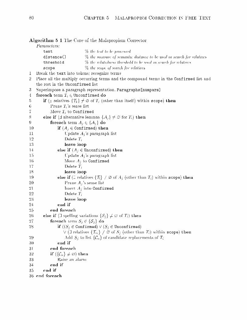
80 Chapter 5. Malapropism Correction in Free Text
Algorithm 5.1 The Core of the Malapropism CorrectorParameters:
text % the text to be processed
distance() % the measure of semantic distance to be used in search for relatives
threshold % the relatedness threshold to be used in search for relatives
scope % the scope of search for relatives
1 Break the text into tokens; recognize terms.2 Place all the multiply occurring terms and the compound terms in the Confirmed list and
the rest in the Unconfirmed list.3 Superimpose a paragraph representation, Paragraphs[numpars].4 foreach term Ti 2 Unconfirmed do
5 if (9 relatives fTkg 6= ? of Ti (other than itself) within scope) then6 Prune Ti's sense list.7 Move Ti to Confirmed.8 else if (9 alternative lemmas fAjg 6= ? for Ti) then9 foreach term Aj 2 fAjg do
10 if (Aj 2 Confirmed) then11 Update Aj 's paragraph list.12 Delete Ti.13 leave loop
14 else if (Aj 2 Unconfirmed) then15 Update Aj 's paragraph list.16 Move Aj to Confirmed.17 Delete Ti.18 leave loop
19 else if (9 relatives fTlg 6= ? of Aj (other than Ti) within scope) then20 Prune Aj 's sense list.21 Insert Aj into Confirmed.22 Delete Ti.23 leave loop
24 end if
25 end foreach
26 else if (9 spelling variations fSjg 6= ? of Ti) then27 foreach term Sj 2 fSjg do28 if ((Sj 2 Confirmed) _ (Sj 2 Unconfirmed)
_ (9 relatives fTmg 6= ? of Sj (other than Ti) within scope) then29 Add Sj to list fCng of candidate replacements of Ti.30 end if
31 end foreach
32 if (fCng 6= ?) then33 Raise an alarm.34 end if
35 end if
36 end foreach
5.3. The New Algorithm 81
term, or a valid token,5 if it is not on the stop-list, does not denote a named entity,
and, in its stemmed form, is present in the system vocabulary (lexicon). Our current
implementation uses a stop-list of 221 closed-class and high-frequency words and a Named
Entity Recognition engine (see Section 5.3.3.2) to weed out high-ambiguity and low-
semantic-content words (e.g., current , dozen, go, must , use, well , 1931 ) and words,
such as names, that are likely to result in spurious connections (e.g., lotus as in Lotus
Development Corporation and hart as in Mr Pete Hart), and to reduce the number of
vocabulary lookups.
A term that has not been invalidated so far is passed to the lookup module, which
checks whether the term, in its original form, is present in the system lexicon by itself or
as the �rst component of a phrase. If it is and there are longer phrases, the corresponding
token is examined along with its successors in the sentence (both in their original and
stemmed form) in an attempt to recognize such a phrase. If the term as it appears in
the text cannot be found in the lexicon, dehyphenation and stemming are attempted.
Because, for the reasons mentioned in Section 2.3.1, the semantic distance measures
implemented all operate only on nominal entries in WordNet, we use the noun portion
of WordNet1.5 as the system vocabulary. The morphology (stemming) module employs
WordNet1.5 routines to recover lemmas of nouns and verbs. Thus, in ected verbs oc-
curring in the text are also considered as long as there exists a noun with an identical
lemma (e.g., walked ! walk , slept ! sleep, etc.).
Each non-compound term starts out as a member of the Unconfirmed list (i.e., the
list of terms that may prove to be malapropos). As the phrase identi�cation process
continues, discovering a new instance of a previously identi�ed term results in the term's
update (see Section 5.3.3.1) and transfer to the Confirmed list (i.e., the list of terms
5No concensus with respect to the relevant terminology is evident from the Computational Linguisticsliterature. In our use, term denotes what is sometimes referred to as word type, while token denotes aspeci�c occurrence, or instance, of a term in text. Also, when the distinction between terms and tokensis unimportant (e.g., in discussions concerning semantic distance), we continue to speak of words as inthe preceding chapters.
82 Chapter 5. Malapropism Correction in Free Text
whose correctness has been ensured; line 2).
To facilitate e�cient access to the physical surroundings (context) of any given word,
an array of lists, Paragraphs[], is introduced in line 3. The element Paragraphs[i] is
a list of (pointers to) all the terms that occur in paragraph i.
Once the initial text representation has been constructed, we proceed to the mala-
propism detection stage. For each originally uncon�rmed term, the system attempts to
�nd one or more terms occurring in its physical vicinity (as determined by scope) that are
semantically nearby according to a given distance measure (line 5; see Section 5.3.3.5
below). If such terms, which we refer to as relatives, exist, the current term is regarded
as having the intended spelling. The term's sense list (see Section 5.3.3.1) is revised
(line 6; see Section 5.3.3.7) and the term itself is decreed con�rmed by placement on the
Confirmed list (line 7).
According to Hirst's conjecture (see Section 5.2), if no relatives can be found, our
term is likely to be a malapropism. Before proceeding to examining its spelling variations,
however, the system attempts to account for a possible case of morphological ambiguity.
This is achieved by subjecting the original form of the given term to another bout of
stemming. If the process produces one or more lemmas di�erent from the one adopted
at �rst (line 8), e.g., axis instead of ax for axes or feel (`an intuitive awareness', etc.)
instead of felt (`a fabric made of compressed matted animal �bers') for felt , every such
lemma (encased in a temporary term) is tested for having duplicates in the text (lines 10
and 14) or related terms (within the scope; line 19). Passing any one of these tests will
serve as a con�rmation of the correctness of its surface form, and the �rst alternative
term Aj that does so will replace the original term Ti (and be moved to Confirmed if not
already there).
If no suitable alternative lemma exists, the suspicion that our term may be a mala-
propism remains and, in order to further investigate it, we examine the term's spelling
variations (line 26; Section 5.3.3.8) in a manner analogous to alternative lemmas (line 28).
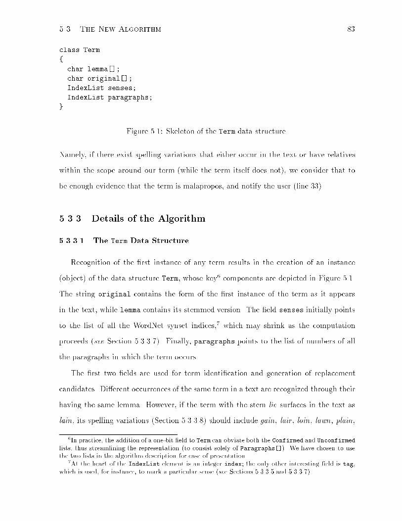
5.3. The New Algorithm 83
class Term
{
char lemma[];
char original[];
IndexList senses;
IndexList paragraphs;
}
Figure 5.1: Skeleton of the Term data structure.
Namely, if there exist spelling variations that either occur in the text or have relatives
within the scope around our term (while the term itself does not), we consider that to
be enough evidence that the term is malapropos, and notify the user (line 33).
5.3.3 Details of the Algorithm
5.3.3.1 The Term Data Structure
Recognition of the �rst instance of any term results in the creation of an instance
(object) of the data structure Term, whose key6 components are depicted in Figure 5.1.
The string original contains the form of the �rst instance of the term as it appears
in the text, while lemma contains its stemmed version. The �eld senses initially points
to the list of all the WordNet synset indices,7 which may shrink as the computation
proceeds (see Section 5.3.3.7). Finally, paragraphs points to the list of numbers of all
the paragraphs in which the term occurs.
The �rst two �elds are used for term identi�cation and generation of replacement
candidates. Di�erent occurrences of the same term in a text are recognized through their
having the same lemma. However, if the term with the stem lie surfaces in the text as
lain, its spelling variations (Section 5.3.3.8) should include gain, lair , loin, lawn, plain,
6In practice, the addition of a one-bit �eld to Term can obviate both the Confirmed and Unconfirmed
lists, thus streamlining the representation (to consist solely of Paragraphs[]). We have chosen to usethe two lists in the algorithm description for ease of presentation.
7At the heart of the IndexList element is an integer index; the only other interesting �eld is tag,which is used, for instance, to mark a particular sense (see Sections 5.3.3.5 and 5.3.3.7).
84 Chapter 5. Malapropism Correction in Free Text
etc., and not die, lee, life, lieu, and pie. Notice that we only need to store the surface
form of the �rst instance in original, as spelling variations are never generated for terms
that occur in the text more than once.
The last two �elds are relied upon in relatedness computations (see Section 5.3.3.5).
Also, it is the �eld paragraphs that is updated when a new instance of a term is encoun-
tered.
5.3.3.2 Named Entities
As we mentioned in Section 5.3.2, our malapropism-correction system, in an attempt to
reduce the number of spurious associations, incorporates a module for �ltering out proper
names. In the current implementation, the module, based on a Lexical Analyzer gener-
ously made available to us by Dekang Lin and Nalante Inc., functions as a preprocessor,
making a pass through a given text and submitting its output to the rest of the system.
Sentence (2), for instance, is thus transformed into (20), which subsequently undergoes
the procedure of valid-term extraction by means of stop-list and vocabulary lookup.
(2) Weather permitting, Mr. Russell commutes every day from his Novato, Calif.,
home in his single-engine airplane.
(20) Weather permitting commutes every day from his home in his single-engine air-
plane .
We will see more examples and some discussion in Section 5.6.1.
5.3.3.3 Compounds
In our special treatment of compounds (line 2), we follow St-Onge's [1995] intuition
that the probability of an accidental formation of a multiword compound (phrase) (e.g.,
abdominal cavity, chief executive o�cer , automated teller machine, withdrawal symptom)
is so low that any such phrase can be regarded as con�rmed through intra-relatedness.
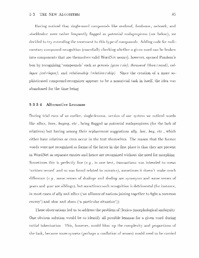
5.3. The New Algorithm 85
Having noticed that single-word compounds like weekend , henhouse, network , and
stockbroker were rather frequently agged as potential malapropisms (see below), we
decided to try extending the treatment to this type of compounds. Adding code for rudi-
mentary compound recognition (essentially checking whether a given word can be broken
into components that are themselves valid WordNet nouns), however, opened Pandora's
box by recognizing `compounds' such as genesis (gene+sis), thousand (thou+sand), col-
lapse (col+lapse), and relationship (relation+ship). Since the creation of a more so-
phisticated compound-recognizer appears to be a nontrivial task in itself, the idea was
abandoned for the time being.
5.3.3.4 Alternative Lemmas
During trial runs of an earlier, single-lemma, version of our system we noticed words
like allies, laws, buying, etc., being agged as potential malapropisms (for the lack of
relatives) but having among their replacement suggestions ally, law , buy, etc., which
either have relatives or even occur in the text themselves. The reason that the former
words were not recognized as forms of the latter in the �rst place is that they are present
in WordNet as separate entries and hence are recognized without the need for morphing.
Sometimes this is perfectly �ne (e.g., in one text, transactions was intended to mean
`written record' and so was found related to minutes), sometimes it doesn't make much
di�erence (e.g., some senses of dealings and dealing are synonyms and some senses of
years and year are siblings), but sometimes such recognition is detrimental (for instance,
in most cases of ally and allies (`an alliance of nations joining together to �ght a common
enemy') and shoe and shoes (`a particular situation')).
These observations led us to address the problem of (lexico-)morphological ambiguity.
One obvious solution would be to identify all possible lemmas for a given word during
initial tokenization. This, however, would blow up the complexity and proportions of
the task, because more synsets (perhaps a con ation of senses) would need to be carried
86 Chapter 5. Malapropism Correction in Free Text
Algorithm 5.2 Search for RelativesParameters:
Tc % the current term
distance() % the measure of semantic distance
threshold % the relatedness threshold
scope % the size of the search scope (scope � numpars)
Paragraphs[numpars] % the paragraph representation of the text
Te % the `exception' term
Result:
set fTrg of Tc's relatives within scope, or within distance of nearest relative if less thenscope
1 fTrg ?
2 back Txc % the paragraph in which Tc occurs (see footnotes 8 and 9)
3 forth Txc
4 while (forth� back � scope) do5 foreach term Ti 2 ((Paragraphs[back mod numpars]
[ Paragraphs[forth mod numpars]) n Te) do6 if (distance(Tc; Ti) < threshold) then7 fTrg fTrg [ Ti8 end if
9 end foreach
10 if (fTrg 6= ?) then11 return fTrg
12 end if
13 back back� 114 forth forth+ 115 end while
16 return ?
around and later discriminated among. Wishing to keep the system real-time, we opted
for computing alternative lemmas on-demand: i.e., if we cannot �nd relatives for, say,
allies or hijacking, we apply morphological routines to �nd ally and hijack as their alter-
native lemmas and, if these have duplicates or relatives, we simply substitute them for
the originally adopted lemmas (instead of regarding the latter as potential malapropisms
and looking for spelling variants).
5.3.3.5 Search for Relatives
Algorithm 5.2 outlines the method used to �nd terms related to the given term Tc
according to the given algorithm for measuring semantic distance distance. A pair
5.3. The New Algorithm 87
of terms is considered related if the semantic distance between them is less then the
relatedness threshold threshold (see line 6).
The idea behind the method is to check every term (other than the `exception' term
Te) in the vicinity of the given term Tc for being semantically close to Tc while progres-
sively enlarging the vicinity, until either the size of the vicinity exceeds a given limit
(scope; line 4) or a semantically close term is found (line 10). In the latter case, for the
reasons to be explained in Section 5.3.3.7, the procedure does not terminate until it has
collected all of the semantically related terms that are within the same physical distance
from Tc as the �rst one discovered.
The size of the search scope scope is given in paragraphs, and the text is thought
of as a closed circuit, i.e., the last paragraph is taken to precede the �rst and the �rst
paragraph to follow the last (line 5). Array Paragraphs[] (see Section 5.3.2) is used
to access all the terms occurring in a given paragraph, and the search begins at the8
paragraph in which Tc occurs (lines 2 and 3).9
Looking back at Algorithm 5.1, we can understand the meaning of the �nal parameter,
Te: when searching for relatives of an original term (Algorithm 5.1, line 5), we do not
want to relate it to itself, and, when looking for relatives of an alternative-lemma term
(line 19) or a spelling-variation term (line 28), we should ignore the original term.
5.3.3.6 Semantic Distance Between Terms
As was discussed in Chapter 2, measures of semantic distance or relatedness are typi-
cally de�ned on a domain of concepts. In particular, the measures implemented for our
malapropism corrector (see Section 5.4.1) were meant to operate on nominal concepts
of WordNet (represented therein by synsets). As we alluded to in the same chapter,
however (see, for instance, Section 2.4.1), such measures can be naturally extended to
8 Being an uncon�rmed term, Tc cannot occur in more than one paragraph.9 In terms of the Term data structure, T x
c is nothing but the �rst (and only) element of Tc.paragraphs.
88 Chapter 5. Malapropism Correction in Free Text
operate on words (terms): given a function distance(si; sj) that computes semantic dis-
tance between the synsets si and sj (according to some measure), we can de�ne semantic
distance between two terms Tl and Tm to be
distance(Tl; Tm) = minsl2Tl:senses;sm2Tm:senses
[distance(sl; sm)] ; (5.1)
that is, the distance between their semantically closest senses.
5.3.3.7 Pruning
Referencing Algorithm 5.2 back to Algorithm 5.1, we notice that what the actual relatives
of a given term are is unimportant so long as the term has them. (Thus, the search for
relatives is described as returning the set fTrg chie y for the sake of presentation.) What
may be useful, on the other hand, is the set fSig of the senses of the current term Tc
that have resulted in its being considered related to terms within the search scope. In
terms of Equation 5.1, these are the synset indices sl that deliver the minimum to the
right-hand side of the equation (i.e., [argRHS]1) when Tc takes the place of Tl and Tm
ranges over the members of fTrg. Pruning of a term's sense list (referred to in lines 6
and 20 of Algorithm 5.1) then consists in replacing the term's current sense list with the
list fSig (which is, of course, a sublist of the former).
The main practical reason for pruning is to reduce the number of subsequent com-
putations of concept-distance. That is, according to Algorithm 5.2, after it has been
con�rmed by virtue of having relatives, a given term Ti will still participate in the term-
distance computations at least for any uncon�rmed term Tj that comes after it in the
same paragraph (one paragraph being the smallest scope size). Since any distance com-
putation involving Ti entails concept-distance computations for each of Ti's current senses
(see Equation 5.1), then, if its sense sik was not included in fSig, either it must have
not delivered the value of distance(Ti; Tj) or it did, but the value exceeded the related-
5.3. The New Algorithm 89
ness threshold.10 In either case, due to the symmetry of distance, sik will not result in
anything useful in the computation of distance(Tj; Ti) either.
Semantically speaking, sense-list pruning amounts to partial disambiguation. This
stand on pruning has actually a�ected certain design decisions. Namely, as was mentioned
in Section 5.3.3.5, if the system discovers the �rst related term, say, in the paragraph
preceding the current token, it will continue scanning the �1-paragraph vicinity of the
current token (i.e., both the preceding and the following paragraph) just in case there
are any other terms within the relatedness threshold. The reason for this is that while
we are willing to assume that a term's neighborhood helps resolve the ambiguity of its
meaning, we are not willing to put one particular related term from this neighborhood
(whose size is measured in paragraphs) above the others (i.e., if instances of two terms
related to a given term occur in the same paragraph, their physical distances from the
given term are the same and hence their contributions to its disambiguation should be
equal).
Note that, aside from the aforementioned savings in computation, pruning can have
disambiguation-related e�ects when it comes to checking relatedness of other terms'
spelling variations and of terms surfacing farther from a given term than its nearest
relatives.11
In the implementation, pruning can be facilitated either by tagging the signi�cant
sense of Tc in the process of computing distance(Tc; Ti) (see footnote 7 on page 83) and
preserving the tag if the resulting value is less than the threshold or by adding a �eld to
the Term data structure that would contain the signi�cant sense of Tc for each member
of fTrg.
10That is, mathematically, either 8sjl 2 Tj:senses (9sim 2 Ti:senses n fsikg (distance(sim; sjl) <distance(skm; sjl))) or 8sjl 2 Tj :senses (distance(skm; sjl) � distance(Ti; Tj) � threshold) .
11In both cases, Tc's sense that has been eliminated could have signi�cance for distance(Sj; Tc) ordistance(Tk; Tc) because neither distance(Tc; Sj) nor distance(Tc; Tk) has ever been computed.
90 Chapter 5. Malapropism Correction in Free Text
5.3.3.8 Spelling Variations
Following St-Onge, we use routines from the popular Unix spelling checker ispell12 to
generate a list of \near misses" (\words which di�er by only a single letter, a missing or
extra letter, a pair of transposed letters, or a missing space or hyphen" [man page]) for
the original form of a given term Tc that has been agged as a potential malapropism.
Those elements of this list that satisfy the validity condition (see Section 5.3.2) and are
not a morphological variation of Tc's lemma give rise to the spelling-variation terms Sj
referred to on lines 26{29 of Algorithm 5.1.
5.3.3.9 Alarms and Related Issues
The exact sequence of actions summarized as \raising an alarm" on line 33 of Algo-
rithm 5.1 should depend on the mode of the program's execution.
It appears sensible to o�er the list fCng of candidate replacements, perhaps even
ranked in order of their semantic proximity to the context. If the session is interactive,
the user will then be able to either choose a replacement from the list or type in his/her
own. Either action will validate the alarm and should result in replacement of the original
term with the correction (and subsequent con�rmation (inclusion into Confirmed) of
the latter). Naturally, the user may alternatively choose to con�rm the spelling of the
original term, thereby invalidating the alarm. This action should, obviously, result in the
con�rmation of the original term.13
If the program is run in batch-mode, on the other hand, we do not have the luxury
of a user's con�rmation of either spelling or correction. In this case, there is no foolproof
way of discriminating among the replacement candidates, and hence they should not be
12International Ispell Version 3.1.08 05/24/94; Copyright c 1983 Pace Willisson; International versionCopyright c 1987, 1988, 1990, 1991, 1992, 1993 Geo� Kuenning
13If execution speed were at premium, we could opt for raising an alarm as soon as we come acrossthe �rst spelling variation that passes the test on line 28 of Algorithm 5.1 and having the user eithertype in a replacement or con�rm the original spelling, without o�ering a list of suggestions.
5.4. System Parameters 91
substituted in. We do, however, have a choice of either removing terms that have been
declared as malapropisms from the text representation or leaving them therein. The
main e�ect of selecting the former option is similar to that of pruning (Section 5.3.3.7):
savings in computation. If an alarm-bearing term remains in the representation, on the
other hand, it is possible that a spelling correction for another term will turn out to be
related to it. However, at least within the single-pass sequential processing paradigm, we
will not be able to take advantage of this (and, for instance, annul the alarm).14
5.4 System Parameters
As is evident from Algorithm 5.1 (Section 5.3.2), there are three principal parameters to
the malapropism corrector: the method of measuring semantic distance (distance), the
relatedness threshold (threshold), marking the boundary between the related and unre-
lated terms, and the scope of search for related terms (scope). The following subsections
discuss each of these in turn.
5.4.1 Measures of Semantic Distance
Due to time and resource constraints, we were able to implement only a subset of the
semantic relatedness measures presented in Chapter 2. We decided to focus our e�orts on
measures that use WordNet as their knowledge source and admit of a fairly straightfor-
ward rendition as functions in a programming language. As a result, six measures were
implemented as plug-ins for the malapropism correction system: Hirst and St-Onge's
(Section 2.3.2.2), Jiang and Conrath's (Section 2.4.2), Leacock and Chodorow's (Sec-
tion 2.3.3.3), Lin's (Section 2.4.3), Resnik's (Section 2.4.1), and Sussna's (Section 2.3.3.1).
14Similar considerations apply to malapropism-suspects that do not result in an alarm due to theirlack of candidate replacements.
92 Chapter 5. Malapropism Correction in Free Text
5.4.1.1 Distance vs Relatedness
A careful reader may have noticed that, up to this point in our discussion of the algorithm,
we have been talking about distancedespite the fact that four out of the six implemented
measures, by design, return a relatedness value. Conceptually, as was alluded to in
Section 1.2, this presents no problem thanks to the inverse relation between the two
notions: distance = max(relatedness) � relatedness and conversely. Computationally,
however, the conversion may at times be di�cult to perform: for instance, in Resnik's
case, max(relatedness) is 1.
Therefore, in our actual implementation, we kept the original type of each measure
(i.e., relatedness or distance) and simply associated a di�erent threshold-comparison oper-
ator with either type. As a result, in cases of relatedness measure, line 6 of Algorithm 5.2
(Section 5.3.3.5) would translate into
if (relatedness(Tc; Ti) > threshold) then .
5.4.1.2 Implementation Notes
Extra-Strong Relations As described in Section 5.3.2, any term occurring more than
once in a given text is considered to have the intended spelling without further examina-
tion of its context(s). This is identical to Hirst and St-Onge's identi�cation of extra-strong
relations and is supported, for instance, by Pollock and Zamora's [1983] �ndings that,
with the exception of a handful of frequently misspelled words, misspellings rarely tend
to be repeated.15
Corpus of Empirical Data Although, in their original experiments, Lin [1997b] and
Jiang and Conrath [1997] used SemCor [Miller et al., 1993], a sense-tagged subset of the
Brown Corpus, as their corpus of empirical data, we decided to follow Resnik [1995] and
15Pollock and Zamora used a 25-million-word corpus of scienti�c and scholarly writings from chemistryfor their analysis.
5.4. System Parameters 93
use the (full and untagged) Brown Corpus (Section 2.4.1) for obtaining the frequency
counts of WordNet concepts. While choosing the Brown Corpus over SemCor essentially
meant trading accuracy for size, it is our belief that using a non-disambiguated corpus
constitutes a more general approach. The availability of disambiguated texts such as
SemCor is highly limited, due to the fact that automatic sense-tagging of text remains
an open problem of NLP and manual sense-tagging of large corpora is prohibitively labor-
intensive. On the other hand, the volume of `raw' textual data in electronic form has been
steadily growing with the development of the Internet. Hence, we may treat the empirical-
data corpus as yet another system parameter and use di�erent corpora to �ne-tune the
performance according to genre or other criteria without additional expenditures.
Hirst and St-Onge's Method We followed St-Onge and Green (personal commu-
nication) in setting C to 100 and k to 2 in Equation 2.8. Furthermore, for reasons of
e�ciency, we adopted Green's modi�cation of Hirst and St-Onge's criteria of strong
relatedness: cases
2. the two words are associated with two di�erent synsets which are
connected by a horizontal link
and
3. \there is any kind of link at all between a synset associated with each
word" but one word is a compound that includes the other
were replaced by
20. the two words are associated with two synsets which are connected by
a single link.
Finally, with respect to numerical values, we took our own suggestion (end of Sec-
tion 2.3.2.2) but di�erentiated between the two kinds of strong relations, corresponding
94 Chapter 5. Malapropism Correction in Free Text
to 0 links and 1 link between synsets, by giving the weight of 2C (200) to the former and
1:5C (150) to the latter.16 As can be seen from Section 5.4.2, this distinction is of no
consequence in the framework of the present system. However, it adds an extra grade to
the scale of Hirst and St-Onge's measure (which may prove useful in other applications).
Jiang and Conrath's Method Owing to the relative insigni�cance of values of Equa-
tion 2.28 parameters within the best-performance range (Section 2.4.2), we implemented
the simplest form of Jiang and Conrath's formula for semantic distance as given by
Equation 2.30.
Sussna's Method One of the key constituents of Sussna's measure of semantic dis-
tance (Section 2.3.3.1) is the depth d of a given edge (see Equation 2.10). Sussna equates
it with the depth of the deeper of the edge's end-nodes, where a node's depth is deter-
mined as follows. Picture the entire noun network of WordNet as a tree. It is rooted in
an extrinsic node posited above the unique beginners (see Section 2.3.1), and parentage
in the tree is by way of any upward relation as well as antonymy. The depths are then
\determined recursively as one descends into the tree" [Sussna, 1997]. For a node without
an antonym, depth is taken to be one more than the average depth of all of the node's
hypernyms and holonyms. Formally,
d(c) =1
m
mXi=1
d(pari(c)) + 1 ; (5.2)
where c is the given node and the pari(c), 1 � i � m,are its m parents. If a node
does have an antonym, however, \the antonym can be considered as parent and child
simultaneously". The depth of such a node is then \de�ned to be the average of two
quantities: one more than the average depth of its parents via non-antonymy links, and
16In the light of this scheme, Green's simpli�cation then mathematicallymeans altering the relatednessvalue of all the pairs of concepts that are one vertical link apart but are not related lexically from C � 1to 1:5C.
5.4. System Parameters 95
two more than the average depth of the parents of its antonym", or
d(c) =1
2
" 1
m
mXi=1
d(pari(c)) + 1
!+
1
n
nXj=1
d(parj(ant(c))) + 2
!#: (5.3)
Unfortunately, in the course of our attempt at reimplementing Sussna's measure, we
ran into two problems which eventually forced us to abandon it.
The �rst has to do with the number of antonyms. Presumably because it was true
of the (earlier) version of WordNet that Sussna worked with, his methodology for the
depth calculation presupposes uniqueness of an antonym for a given node. In Word-
Net1.5, however, this premise no longer holds. For instance, extroversion (`an extroverted
disposition; concern with what is outside the self') has both introversion (`an introverted
disposition; concern with one's own thoughts and feelings') and ambiversion (`a balanced
disposition intermediate between extroversion and introversion') as its antonyms, and dis-
obedience/noncompliance has both conformity/conformation/compliance/abidance (`acting
according to certain accepted standards') and obedience.17
Formula (5.3) clearly doesn't account for the case of multiple antonyms| but perhaps
it could be modi�ed in an intuitive way; for example:
d(c) =1
2
" 1
m
mXi=1
d(pari(c)) + 1
!+
1
s
sXk=1
1
nk
nkXj=1
d(parj(antk(c))) + 2
!#: (5.4)
The other problem manifested itself as an in�nite loop during an attempted depth
computation. The subsequent investigation revealed that, while the WordNet is-a and
part-of hierarchies, by themselves, are both proper directed acyclic graphs, the graph
resulting from their merging contains cycles (circuits). For instance, burnt sienna (`a
reddish-brown pigment produced by roasting sienna') is-a sienna (`an earth color con-
taining ferric oxides; used as a pigment'), while, at the same time, sienna part-of burnt
17The second example is actually a little more subtle than the �rst. The creators of WordNet realizedearly on that \antonymy is a lexical relation between word forms, not a semantic relation betweenword meanings" [Miller et al., 1990]. Thus, what we really have in the second example is disobedienceopposite-of obedience and noncompliance opposite-of compliance. In Sussna's work, however, thereis no indication of its being treated di�erently from true inter-concept relations like hypernymy orholonymy.
96 Chapter 5. Malapropism Correction in Free Text
sienna. Similarly, corolla (`the petals of a ower collectively forming an inner oral en-
velope or layer of the perianth') is-a petal (`part of the perianth that is usually brightly
colored') while petal part-of corolla.
At present, we are not certain how Sussna's algorithm should be amended in order
to be able to handle situations like these.18
5.4.2 Threshold Determination
While, as we argue in Section 6.1.2, a numerical expression of concept proximity is
desirable for a number of applications, our task at hand, at its top level, requires merely
a binary response: given a pair of terms, we would like to know whether they are related
or not.
The simplest way of mapping a continuum (or even a �nite number) of (comparable)
values onto a set consisting of only two values, say, f0; 1g, is by selecting a single point
(call it a threshold) in the original domain and mapping all the points on one side of this
threshold to 0 and the rest to 1. This is the approach we decided to take in our work.
Notice that, of the �ve measures of relatedness ultimately used in the experiments,
Hirst and St-Onge's constitutes a special case in that the distinction between related and
unrelated concepts is inherent in its de�nition (see Section 2.3.2.2): any pair of weakly
related concepts is considered unrelated. Hence, Hirst and St-Onge's threshold is 0.
For the remaining four measures, thresholds had to be derived. In order to zero in on
a method of doing that, we decided to use the following criteria: �rst, the threshold for
each measure should be linguistically sound; second, the thresholds should be comparable
with one another, i.e., the classi�cations of concepts into related and unrelated produced
by the di�erent measure-threshold pairs should agree to the largest extent possible.19
18Possibilities include calculating depths for each hierarchy separately and then combining (e.g., aver-aging) the results or even ignoring one of the hierarchies altogether. Following either suggestion, however,would constitute a signi�cant deviation from the original approach.
19In the ideal case, then, the measure-threshold pairs would entirely agree with human judgement andwith each other.
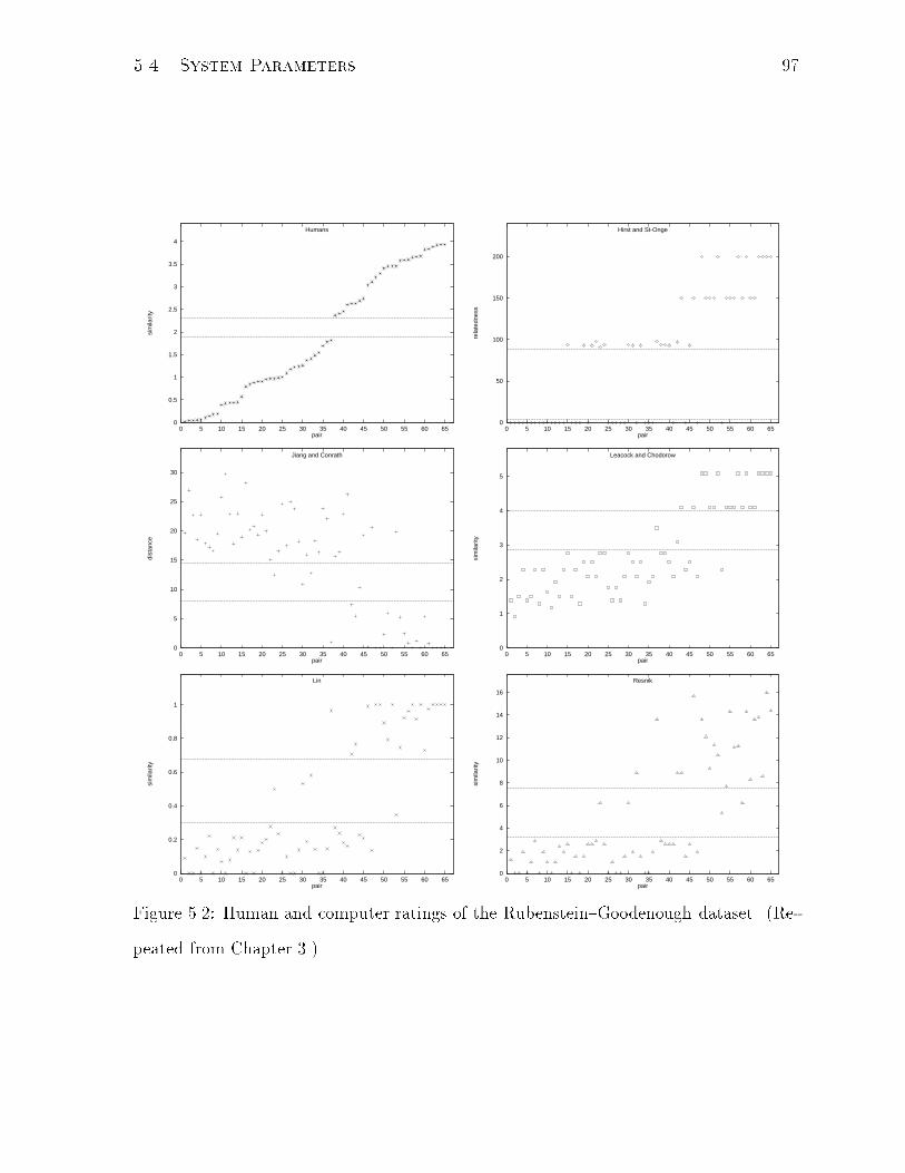
5.4. System Parameters 97
0
0.5
1
1.5
2
2.5
3
3.5
4
0 5 10 15 20 25 30 35 40 45 50 55 60 65
sim
ilarit
y
pair
Humans
0
50
100
150
200
0 5 10 15 20 25 30 35 40 45 50 55 60 65
rela
tedn
ess
pair
Hirst and St-Onge
0
5
10
15
20
25
30
0 5 10 15 20 25 30 35 40 45 50 55 60 65
dist
ance
pair
Jiang and Conrath
0
1
2
3
4
5
0 5 10 15 20 25 30 35 40 45 50 55 60 65
sim
ilarit
y
pair
Leacock and Chodorow
0
0.2
0.4
0.6
0.8
1
0 5 10 15 20 25 30 35 40 45 50 55 60 65
sim
ilarit
y
pair
Lin
0
2
4
6
8
10
12
14
16
0 5 10 15 20 25 30 35 40 45 50 55 60 65
sim
ilarit
y
pair
Resnik
Figure 5.2: Human and computer ratings of the Rubenstein{Goodenough dataset. (Re-
peated from Chapter 3.)
98 Chapter 5. Malapropism Correction in Free Text
Re ection upon the above requirements led us to turn to the experimental results
of similarity rankings presented in Section 3.3. As we pointed out in the course of
analysis of Section 3.3.1, the graphical representation of human similarity-rankings for
the Rubenstein{Goodenough dataset (see Figure 5.2) exhibits a horizontal band in the
vicinity of sim = 2 (the center of the medium-similarity region, separating the pairs
magician{oracle (37) and crane{implement (38)) that contains no points. On the graphs
of computed rankings, to these empty regions correspond bands with only a few (2{4)
points.
This initial observation makes it reasonable to conclude that the boundary between
the related and the unrelated will lie within the identi�ed uncertainty regions for all the
computational measures.20 We now have to take a look at each pair in (and about) the
uncertainty regions.
Since the pair crane{rooster (32) appears in the positive region of Resnik's measure,
we shall include it in the positive regions of both Jiang{Conrath and Lin.21 For Jiang
and Conrath's measure, this single manipulation suggests setting the threshold at 13.
With such a threshold, both mound{shore (23) and coast{hill (30) will end up in the
Jiang{Conrath positive region, and, by induction, in the positive regions of Lin's and
Resnik's.22 For the latter, this will result in the inclusion of implement{tool (58) into
the positive region. (The fact that the pair already belongs to the positive regions of
the other three measures corroborates the correctness of the last decision.) The pair
20We will refer to the regions containing the former two groups of pairs as the positive and negativeregion, respectively. Note, that for Jiang and Conrath's measure, which is a distance, the positive regionlies below negative.
21The reader may notice that the same pair lies in the negative region of the Leacock{Chodorowmeasure. As was mentioned in Section 3.3.1, however, due to its pronouncedly discrete nature, Leacock{Chodorow has a tendency to blur distinctions. For instance, in this case, it gives crane{rooster the samesimilarity value as it does automobile{cushion (22), bird{woodland (29), glass{jewel (36), and oracle{sage (41). All of these lie in the negative regions of the other three measures, but a de�nite intervalaway from crane{rooster . We therefore take Resnik evidence over that of Leacock{Chodorow.
22Here again both pairs can be found in the negative region of the Leacock{Chodorow measure, but, asin the previous case, we choose to ignore this piece of evidence, because of the fact that the pairs monk{slave (15), lad{wizard (24), crane{implement (38), and brother{lad (39), all assigned the same similarityvalue by Leacock{Chodorow's measure, all lie in the negative regions of the other three measures.
5.4. System Parameters 99
serf{slave (53), on the other hand, is found in the negative regions of Leacock{Chodorow
and Jiang{Conrath measure, and this suggests that we classify it as unrelated for Lin's
and Resnik's as well. These considerations help us arrive at the threshold value of 0.4 for
Lin's measure and 6 for Resnik's. Finally, we shall include both pairs magician{oracle
(37) and bird{crane (42) in the positive region of Leacock{Chodorow measure, as they
belong to the positive regions of all the other measures. This step will enable us to set
the threshold for Leacock and Chodorow's measure to 3.
5.4.3 Search Scope
The �nal system parameter is the scope of search for related terms.23
In Hirst and St-Onge's system (Section 5.2), the search scope was dependent on the
type of relation: for strong relations, it was limited to 7 sentences, and, for medium-
strong, to 3 sentences. Also, related-term searches for original terms were backwards
only, while for spelling variations they are performed in both directions.
As is evident from the algorithm description, the above rules underwent several mod-
i�cations for our system. First of all, we decided to measure scope in paragraphs rather
than in blocks of sentences, as the paragraph appears to be a more natural unit of seg-
mentation. Second, since four out of our �ve measures of semantic relatedness do not
intrinsically have a division analogous to medium-strong vs strong (and, in e�ect, we
chose to play down this division in case of Hirst and St-Onge's measure as well), we opted
for a uniform scope size. Next, searches in all cases were made bidirectional. Finally, as a
result of a series of observations, we adopted the circular model of text (as mentioned in
Section 5.3.3.5): the last paragraph of a text is viewed as preceding the �rst paragraph
and, correspondingly, the �rst paragraph is viewed as following the last.24
23This does not include looking for duplicates. Following Hirst and St-Onge, multiple instances of thesame term are always recognized throughout the entire text.
24One example that motivated our decision is illustrated by the pair trombone{horn in the passagequoted in Appendix A: the author mentions trombone when talking about Mr. Russell's profession ashe begins the narrative (�rst paragraph); he then comes back to the topic and uses the word horn near
100 Chapter 5. Malapropism Correction in Free Text
Unlike in the problem of threshold determination, where one has to consider a possibly
in�nite number of candidates, only a small number of feasible alternative sizes of search
scope really exist. Hence, we decided to attempt to arrive at an optimum scope(s) by
experiment with the following four sizes: 1 (i.e., only the paragraph containing the token
in question), 3 (the token's own paragraph plus one paragraph in each direction), 5
(analogous), and the entire text. The result of our experiments are discussed in the
following section.
5.5 Performance Evaluation
In order to evaluate the performance of our malapropism corrector and compare the
semantic relatedness measures used as plug-ins, the system was fed the 500 articles from
the Wall Street Journal that were used in Hirst and St-Onge's original experiments (see
Section 5.2). As in their research, a program was used to replace roughly each 200th
valid token (see Section 5.3.2) with a malapropism. Articles too small to warrant such
a replacement (19 in total) were excluded from consideration. We thus ended up with a
corpus of 107,233 valid tokens, 1408 of which were malapropisms.25
5.5.1 Some Terminology
In order to adequately describe the criteria used to evaluate the performance of the
system, a few terms, due to Hirst and St-Onge, need to be introduced.
� Whenever a token has no relatives within a given scope, it is said to be a potential
malapropism.
the conclusion (second last paragraph). In general, it is to be expected that concepts introduced at thestart of a text will often be recapitulated at the end.
25We assume that the originalWSJ, being carefully edited text, contains essentially no malapropismsof its own.
5.5. Performance Evaluation 101
{ If a potential malapropism has at least one spelling variation that does have
a relative within the scope (we shall refer to such spelling variations as
candidate replacements), we say that an alarm is raised.
� Whether or not it results in an alarm, a potential malapropism is a guess.
{ Those guesses that correspond to actual (introduced) malapropisms are
called correct guesses and those that do not are incorrect guesses.
� If an alarm is triggered by a correct guess, it is a true alarm, or a detected
malapropism. Otherwise, it is a false alarm.
� Conceivably, a detected malapropism might or might not have the intended cor-
rection (i.e., the original word that was replaced by a malapropism during the
generation stage) among its candidate replacements. Finally then, we will call
those that do perfectly detected, or corrected, malapropisms.
5.5.2 Performance Measures
St-Onge [1995] puts forth two basic hypotheses which, using the terminology above, can
be paraphrased as follows:
(H1) Words agged as potential malapropisms are (much) more likely to be actual
malapropisms than the rest of the valid words are.
and
(H2) Among potential malapropisms, actual malapropisms are (much) more likely to
result in an alarm than non-malapropisms are.
These hypotheses motivate the �rst two measures of algorithm performance presented
below.
Performance1 is related to the �rst hypothesis:
102 Chapter 5. Malapropism Correction in Free Text
performance1 =(number of correct guessesnumber of malapropisms )
(number of incorrect guessesnumber of non-malapropisms)
: (5.5)
Qualitatively, performance1 in excess of 1 would mean that actual malapropisms are more
likely to be considered to be anomalous in their context (i.e., be agged as potential
malapropisms) than non-malapropisms are.
Performance2 gives us the probability of a correct guess triggering an alarm over that
of an incorrect guess triggering one:
performance2 =( number of true-alarmsnumber of correct guesses )
( number of false-alarmsnumber of incorrect guesses )
: (5.6)
Thus, hypothesis H2 is true if and only if performance2 � 1.
The product of performance1 and performance2 yields the overall detection-perfor-
mance of the algorithm:
performanceD = performance1 � performance2 =( number of true-alarmsnumber of malapropisms)
( number of false-alarmsnumber of non-malapropisms)
:
(5.7)
This expression corresponds to the probability of a malapropism becoming an alarm over
that of a non-malapropism. Naturally, we would like this to be greater than 1 also.
Finally, the correction-performance of the algorithm is given by the proportion of
perfectly detected malapropisms among those detected:
performanceC =number of corrected malapropisms
number of true alarms: (5.8)
A visual examination of the four measures laid out above can give rise to a couple of
remarks at this point. First, with the exception of correction-performance, the mathe-
matical expressions for the measures involve several (more than two) factors. Therefore,
while the end results have nice interpretations, the analysis of the underlying causes and,
consequently, attempts to compare the e�ects of scope and measure may prove rather
5.5. Performance Evaluation 103
involved. Second, one could argue that the user's perception of performance comes only
from alarms. Thus, while the performance measures presented can be suitable for test-
ing the overall validity of a malapropism detection and correction algorithm, the user's
perspective might be better represented by simpler proportions based on alarms.
These observations led us to augment (and, in part, supersede) St-Onge's evaluation
suite with two criteria that constitute the de-facto standard of evaluating retrieval-type
tasks: precision and recall. In the framework of malapropism detection, their general
de�nitions translate into the following:
precision =number of true alarms
number of alarms(5.9)
and
recall =number of true alarms
number of malapropisms(5.10)
We conclude this section by noting that various other quantities of interest may be
expressed through the performance measures already presented. In particular, precision
and recall values for the task of malapropism correction can be obtained by multiply-
ing the corresponding malapropism detection value by the correction performance (see
Equation 5.8).26
26For instance,
precisionC =number of corrected malapropisms
number of alarms
=number of corrected malapropisms
number of true alarms�number of true alarms
number of alarms= performanceC � precision :
104 Chapter 5. Malapropism Correction in Free Text
5.6 Analysis of Results
5.6.1 Some Examples
Before quantifying and analyzing the results of our experiments, we will present a few
illustrations to help the reader become more familiar with the terminology introduced
in Section 5.5.1 and to demonstrate common situations referred to in the subsequent
discussion.
5.6.1.1 Performance on Genuine Malapropisms
We will begin by giving examples of the system's performance on genuine (introduced)
malapropisms.
The malapropism apposition in sentence (3) was, for all but three measure-scope
combinations, perfectly detected by the system, i.e., apposition was not found to be
related to any other term in the search scope and its intended correction, opposition,
was o�ered as a candidate replacement.
(3) But the push in Congress has fallen short in the past, with Mr. Russell's plain
talk helping to lead the apposition.
In fact, in this particular case, opposition was the only candidate replacement, and it was
suggested because it occurred elsewhere in the text. But when given Hirst and St-Onge's
measure and scope sizes 3, 5, and max as the values of its parameters, the system related
apposition to the term relationship27 found in sentence (4) in the following paragraph
and hence it was not even suspected of being a malapropism.
(4) Forewarned, First Interstate, which o�ers American Express Gold cards and trav-
elers checks, is \reevaluating our relationship" with American Express, according
27According to WordNet, apposition (`a grammatical relation between a word and a noun phrase thatfollows') is-a modi�cation/qualifying/limiting is-a grammatical relation is-a linguistic relation is-a relationsubsumes relationship .
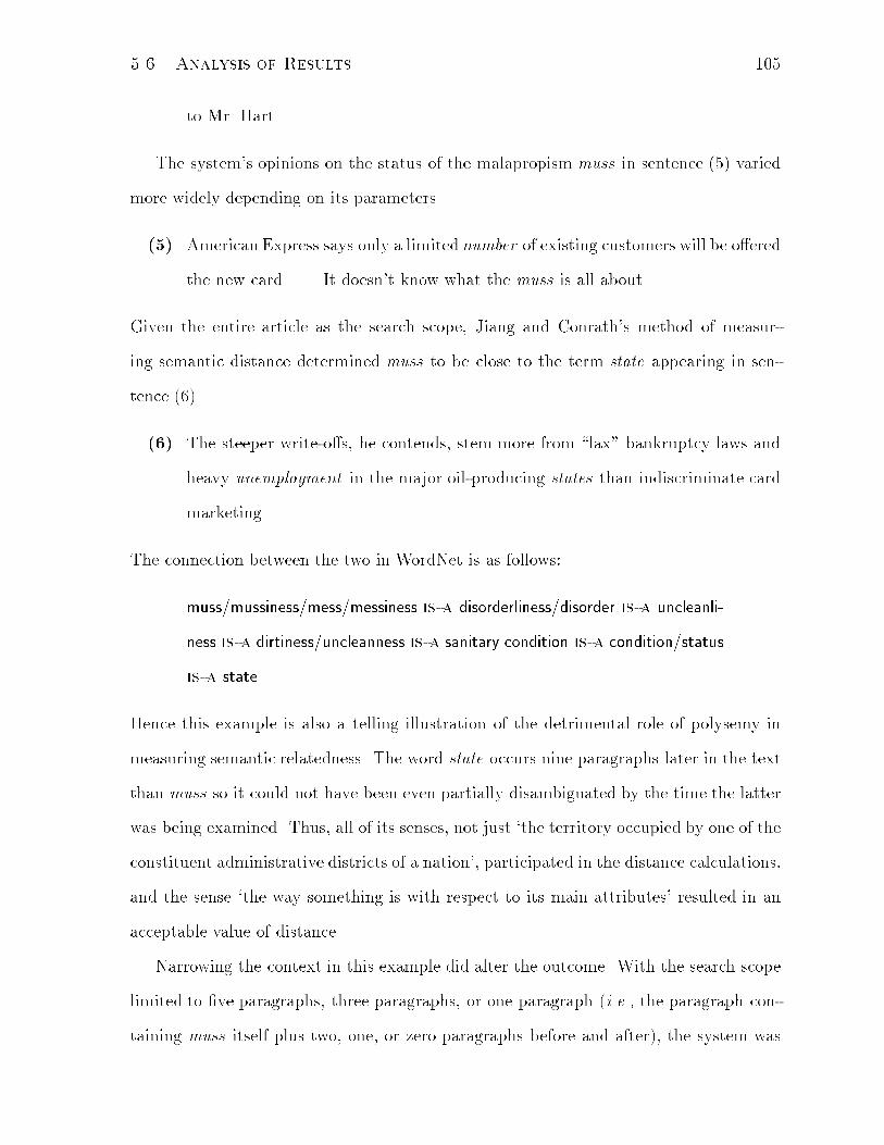
5.6. Analysis of Results 105
to Mr. Hart.
The system's opinions on the status of the malapropism muss in sentence (5) varied
more widely depending on its parameters.
(5) American Express says only a limited number of existing customers will be o�ered
the new card. . . . It doesn't know what the muss is all about.
Given the entire article as the search scope, Jiang and Conrath's method of measur-
ing semantic distance determined muss to be close to the term state appearing in sen-
tence (6).
(6) The steeper write-o�s, he contends, stem more from \lax" bankruptcy laws and
heavy unemployment in the major oil-producing states than indiscriminate card
marketing.
The connection between the two in WordNet is as follows:
muss/mussiness/mess/messiness is-a disorderliness/disorder is-a uncleanli-
ness is-a dirtiness/uncleanness is-a sanitary condition is-a condition/status
is-a state .
Hence this example is also a telling illustration of the detrimental role of polysemy in
measuring semantic relatedness. The word state occurs nine paragraphs later in the text
than muss so it could not have been even partially disambiguated by the time the latter
was being examined. Thus, all of its senses, not just `the territory occupied by one of the
constituent administrative districts of a nation', participated in the distance calculations,
and the sense `the way something is with respect to its main attributes' resulted in an
acceptable value of distance.
Narrowing the context in this example did alter the outcome. With the search scope
limited to �ve paragraphs, three paragraphs, or one paragraph (i.e., the paragraph con-
taining muss itself plus two, one, or zero paragraphs before and after), the system was
106 Chapter 5. Malapropism Correction in Free Text
no longer able to relate muss to anything with Jiang and Conrath's measure. In each
of these cases, however, the term had spelling variations that did have relatives within
the scope (in other words, it had candidate replacements), such as mass, muds, mugs,
and even mess (but in the sense `a large number or amount or extent', in which it was
connected to the term number highlighted in example (5) above), which resulted in a
(true) alarm. Furthermore, for the scope sizes of 3 and 5, the intended correction fuss
was among the candidate replacements, with the term business marked as its relative.
For the scope size of 1, fuss was rejected as a candidate replacement, since business oc-
curred in the following paragraph. Thus, muss constituted a detected malapropism in all
three cases and, in the former two, it was perfectly detected, or corrected.
Other relatedness measures exhibited similar trends with respect to the scope size.
For instance, combining Leacock and Chodorow's measure with the scope sizes 3, 5,
and max resulted in a correction, while combining it with the scope size of 1 only in a
detection. Resnik's measure with the entire text as the scope also enabled the system
to detect the malapropism perfectly, with the scope of 5 or 3 paragraphs imperfectly,
and with the scope of one paragraph the system was not even able to �nd relatives for
spelling variations, hence no alarm was raised, and muss was declared merely a potential
malapropism.
In contrast with the apposition example, the malapropism aw (sentence (7)) was
not even suspected as such by all but �ve measure-scope combinations.
(7) Mr. Russell argues that usury aw depressed rates below market levels years ago,
making current rates seem high.
The Jiang{Conrath, Leacock{Chodorow, and Hirst{St-Onge measures, for instance, all
found aw to be related to the term state (in the same sense (and sentence) as quoted
earlier). The last two measures also related it to level and unemployment (through
state). Lin's measure was not able to make for any of the above connections, but it did
�nd aw close enough to the terms jump and fall , whose instances occur in the preceding
5.6. Analysis of Results 107
paragraph in the article.28 When the system was given Resnik's measure with the scope
sizes of 3, 5, and max and Lin's measure with the scope size 1, however, no relatives were
found for aw , while its spelling correction law already occurred earlier in the text (where
it was con�rmed), so the malapropism was perfectly detected. The system with Resnik's
measure and scope 1, on the other hand, was only able to detect (o�ering replacements
like ow and ak), but not correct the malapropism, since, when its earlier occurrence
was examined, the term law was itself (wrongly) declared a malapropism (and, as a
spelling variation, it did not have any other relatives within aw 's context).
We remark that, as in St-Onge's [1995] case, fully automating the process of mala-
propism generation had the disadvantage of occasionally replacing an original word with
a word that was semantically very close to it: e.g., billion with million, supplier with
supplies, optimist with optimism, raise with rise, or even inquiry with enquiry. While
these would be nearly impossible to detect, one could still argue that they nonetheless
constitute valid examples of malapropisms (in the sense of mimicking human behavior)
and thus should not be excluded from consideration.
5.6.1.2 Performance on Non-malapropisms
We will next look at the system's performance on non-malapropisms (i.e., original, non-
substituted, words in the text). Unlike the preceding examples, the default, and desirable,
case here should be `no alarm'. We will therefore mainly focus on the cases where the
system mis�red.
To a human reader, the word fox in passage (8) would hardly seem out of place, even
if he or she were not familiar with the idiom.
(8) But Mr. Russell is resolute. \Banks need to realize that there is a fox in the
28jump/leap (`an abrupt transition') is-a transition is-a change/alteration/modi�cation,fall/downfall (`a sudden decline in strength or number or importance') is-a weakening is-a transforma-tion/transmutation/shift/qualitative change is-a change/alteration/modi�cation,and change/alteration/modi�cation subsumes damage/harm/impairment subsumes aw/defect.
108 Chapter 5. Malapropism Correction in Free Text
henhouse," he declares. Visa and the 56-year-old Mr. Russell, who enjoys riding
a Harley-Davidsonmotorcycle, have collided with consumers and Congress before.
After all, henhouses are for cultivating hens, and hens and foxes are both animals.
Nevertheless, none of the measures were able to make the connection: while, according
to some, fox is close enough to hen, the latter is too far from henhouse according to all
of the measures. (In fact, it is almost as far from henhouse as fox is.) Roughly one third
of the measure-scope combinations were furthermore unable to relate fox to anything
else either, but were able to come up with candidate replacements such as box (related
to motorcycle, for both are instrumentality/instrumentation (`an artifact (or system of
artifacts) that is instrumental in accomplishing some end')), fob, cox (related to general
in sentence (9) which was taken to be a noun), etc., thereby resulting in a false alarm.
(9) \He is more vociferous, but his statements probably re ect the general thought
of the leading card issuers. . . ."
The system run with the remaining combinations marked fox as a con�rmed term; how-
ever, when the relations underlying these decisions were examined, it turned out that,
in every single case, an inappropriate sense of fox was used. For example, Leacock and
Chodorow's measure found fox to be related to hide, where the latter was an unfortunate
nominalization of the identical-lemma verb and the former was interpreted as the pelt of
a fox. Hirst and St-Onge's measure connected fox to consumer by noticing that, when
the former means fox/dodger/slyboots, both are persons. An even more exotic sense of
the word fox was chosen by Jiang and Conrath's and Lin's measures, which were able to
relate it to question, response, and american:
Fox is-a Algonquin/. . . /Algonquian language is-a Amerind/. . . /American-
Indian language is-a natural language/tongue is-a language/linguistic com-
munication (`a systematic means of communicating by the use of sounds
or conventional symbols') ,
5.6. Analysis of Results 109
question/interrogative/interrogative sentence is-a sentence is-a string of
words/. . . /linguistic string is-a language/linguistic communication
(and similarly for response/reply/answer), and
American/. . . /American English is-a English/English language is-a West
Germanic language . . . is-a Germanic language . . . is-a Indo-European
language . . . is-a natural language/tongue .
This example also lets us say a few more words about the named-entity recognition
component of the system. All of the sample sentences above have been reproduced as
they appear in original documents (except for the malapropism substitutions). After
preprocessing by the Named Entity Recognition engine (see Section 5.3.3.2), however,
passage (8), for instance, would become
(80) But is resolute . Need to realize that there is a fox in the henhouse he declares
. Visa and the 56-year-old who enjoys riding a motorcycle have collided with
consumers and Congress before .
(which would be reduced even further during the validation stage). As we can see, we
have gotten rid of a couple of noise words, such as Harley-Davidson, Mr , and Russell ,
the last of which could result in another unwanted connection similar to fox{consumer ,
because it happens to be in the WordNet lexicon with a single sense Russell/. . . /Bertrand
Russell which is subsumed by person/individual/. . . . However, the transformation has not
been perfect. On the one hand, we have lost an occurrence of the term bank , which
must have been mistaken for a last name (presumably due to its position and frequency);
on the other hand, the term Visa has not been recognized as a proprietary name (even
though Visa International , occurring elsewhere in the document, was). Likewise, the
term American Express was winnowed by the system throughout the document, but not
when it surfaced in American Express Gold cards | and this is where the term american
from the very last relation example came from.
110 Chapter 5. Malapropism Correction in Free Text
69 just checking
The following example was alluded to in Section 5.4.3 where we attempted to mo-
tivate the circular model of text. For the scope sizes of 1 and 3, the word trombone
in sentence (10) occurring in the very �rst paragraph of the article, was marked as a
potential malapropism by the system.
(10) Charles T. Russell used to play trombone in Pittsburgh burlesque houses and
with big bands in the Southeast.
When the scope was increased to 5, however, the article's second last paragraph, con-
taining sentence (11) became a part of the context, and the Leacock{Chodorow, Resnik,
and Hirst{St-Onge measures were able to make the desired connection.
(11) Like scores of musicians, he put down his horn when television arrived in the
1950s.
Having decided to investigate the reasons why the other two measures failed to do so, we
discovered that the probability of concept trombone is zero, as there are no occurrences of
the word trombone (or its sole subordinate sackbut) in the Brown Corpus (which was used
to derive the probabilities; see Section 5.4.1.2). Since the expression for Lin's similarity
contains the (negative) logarithm of this probability in its denominator (Equation 2.34,
Section 2.4.3) and the expression for Jiang and Conrath's distance contains the same term
as a part of a sum (Equation 2.30, Section 2.4.2), the value of the former, for trombone
and horn, came out in�nitely small (i.e., essentially zero) and that of the latter in�nitely
large. Obviously, the values of the Leacock{Chodorow or Hirst{St-Onge measures were
not a�ected as they are edge-based (see Section 2.4.2), but nor was that of Resnik's,
since it only makes use of the lowest superordinate of the two concepts (brass), which in
this case had a non-zero probability.
As the reader may have noticed, of the �ve measures participating in the experiments,
only Hirst and St-Onge's can take advantage of WordNet relations other than is-a. Our
5.6. Analysis of Results 111
�nal example is intended to demonstrate how this distinction can a�ect the behavior of
the system. Let us come back, one last time, to sentence (12).
(12) \Banks need to realize that there is a fox in the henhouse," he declares.
As we have seen earlier, none of the relatedness measures were able to see the connection
between henhouse and fox . It should therefore be expected that the former be declared
a potential malapropism. In e�ect, this is what happened with every measure except
Hirst and St-Onge's, which, when given to the system, enabled it to detect a relationship
between henhouse and the word ceiling from sentence (13) since
henhouse/. . . /chicken coop is-a farm building is-a building/edi�ce has-a
room has-a ceiling .
(13) As in past years, Congress is currently considering imposing rate ceilings, and
some consumer groups think such a law would be an appropriate response to
Mr. Russell's recent harangue.
5.6.2 St-Onge's Performance Measures
A summary of the results with respect to several performance criteria introduced in Hirst
and St-Onge's [1998] original malapropism detection and correction research is given in
Table 5.1 and Figures 5.3 and 5.4.
For the reasons discussed in Section 5.5.2, we will restrict our analysis to merely mak-
ing a couple of remarks. All the values of performance1, performance2, and performanceD
are greater than 1, as desired. Figures within each category are similar overall in magni-
tude and compare fairly well with Hirst and St-Onge's original results.30 The corrective
29The results given under the heading chains, here and onwards, are those of Hirst and St-Onge'slexical-chain-based system (Section 5.2).
30It should be noted that all of the �gures in Table 5.1 are but single data-points, as opposed tostatistical means of some sort. Thus, we cannot make any de�nite judgements concerning their compar-ison, any apparent trends (e.g., with respect to scope), or the like. In order to do so, we would have
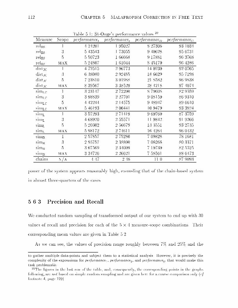
112 Chapter 5. Malapropism Correction in Free Text
Table 5.1: St-Onge's performance values.29
Measure Scope performance1 performance2 performanceD performanceCrelHS 1 4.24201 1.95027 8.27306 93.1034relHS 3 5.43543 1.73055 9.40628 95.6731relHS 5 5.50723 1.66668 9.17881 96.3768relHS max 5.24807 1.61044 8.45170 96.4286distJC 1 4.72515 2.96773 14.0230 92.0705distJC 3 6.38080 2.92485 18.6629 95.7198distJC 5 7.23810 3.01988 21.8582 96.9838distJC max 8.39567 3.38529 28.4218 97.4074simLC 1 3.23147 2.72200 8.79608 82.9559simLC 3 3.98839 2.27701 9.08159 86.9310simLC 5 4.42244 2.14575 9.48947 89.6610simLC max 5.46193 2.00441 10.9479 93.3824simL 1 3.57293 2.71419 9.69760 87.3759simL 3 4.68920 2.55571 11.9842 91.9266simL 5 5.20302 2.56679 13.3551 93.2735simL max 5.98172 2.74611 16.4264 96.0432simR 1 2.57857 2.75280 7.09828 78.1681simR 3 2.95757 2.38800 7.06266 80.3371simR 5 3.07569 2.34009 7.19739 82.5525simR max 3.34726 2.26621 7.58561 88.6473chains n/a 4.47 2.46 11.0 87.9093
power of the system appears reasonably high, exceeding that of the chain-based system
in almost three-quarters of the cases.
5.6.3 Precision and Recall
We conducted random sampling of transformed output of our system to end up with 30
values of recall and precision for each of the 5 � 4 measure-scope combinations. Their
corresponding mean values are given in Table 5.2.
As we can see, the values of precision range roughly between 7% and 25% and the
to gather multiple data-points and subject them to a statistical analysis. However, it is precisely thecomplexity of the expressions for performance1, performance2, and performanceD that would make thistask problematic.
31The �gures in the last row of the table, and, consequently, the corresponding points in the graphsfollowing, are not based on simple random sampling and are given here for a coarse comparison only (cffootnote 4, page 129).
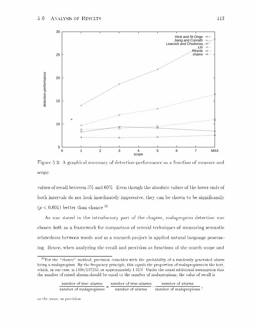
5.6. Analysis of Results 113
5
10
15
20
25
30
0 1 2 3 4 5 6 7 MAX
dete
ctio
n-pe
rfor
man
ce
scope
Hirst and St-OngeJiang and Conrath
Leacock and ChodorowLin
Resnikchains
Figure 5.3: A graphical summary of detection-performance as a function of measure and
scope.
values of recall between 5% and 60%. Even though the absolute values of the lower ends of
both intervals do not look inordinately impressive, they can be shown to be signi�cantly
(p < 0:001) better than chance.32
As was stated in the introductory part of the chapter, malapropism detection was
chosen both as a framework for comparison of several techniques of measuring semantic
relatedness between words and as a research project in applied natural language process-
ing. Hence, when analyzing the recall and precision as functions of the search scope and
32For the \chance" method, precision coincides with the probability of a randomly generated alarmbeing a malapropism. By the frequency principle, this equals the proportion of malapropisms in the text,which, in our case, is 1408=107233, or approximately 1.31%. Under the usual additional assumption thatthe number of raised alarms should be equal to the number of malapropisms, the value of recall is
number of true alarms
number of malapropisms=
number of true-alarms
number of alarms�
number of alarms
number of malapropisms;
or the same as precision.
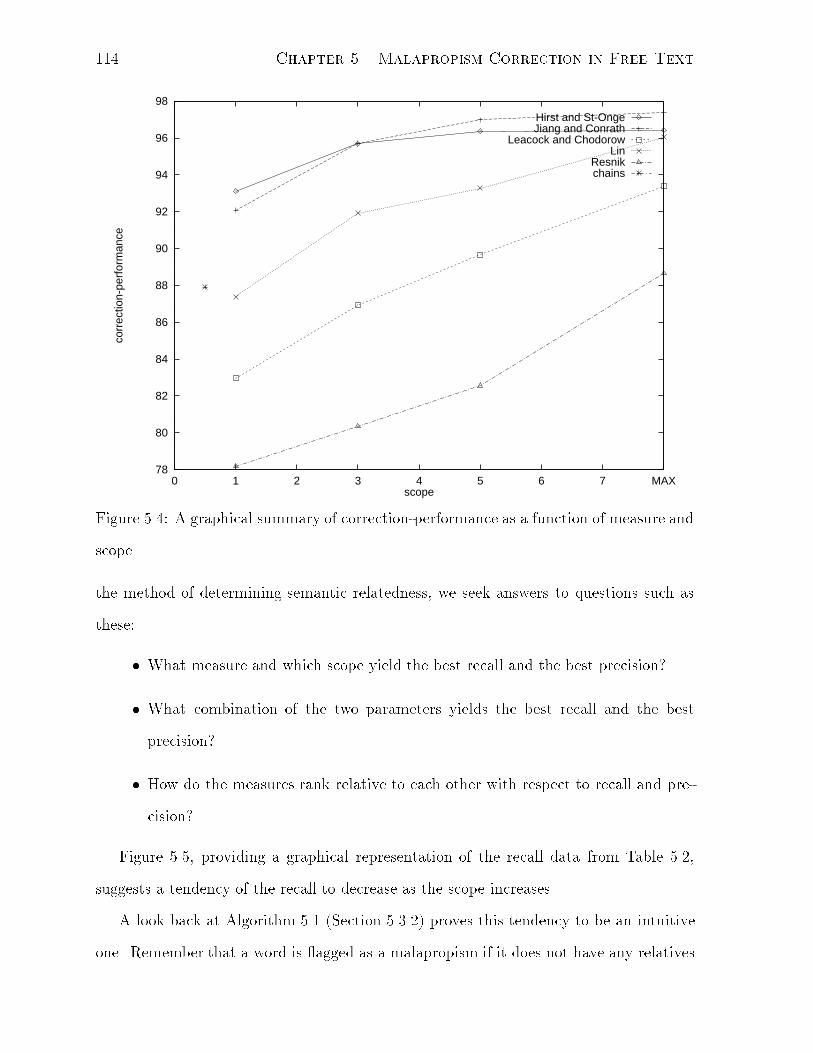
114 Chapter 5. Malapropism Correction in Free Text
78
80
82
84
86
88
90
92
94
96
98
0 1 2 3 4 5 6 7 MAX
corr
ectio
n-pe
rfor
man
ce
scope
Hirst and St-OngeJiang and Conrath
Leacock and ChodorowLin
Resnikchains
Figure 5.4: A graphical summary of correction-performance as a function of measure and
scope.
the method of determining semantic relatedness, we seek answers to questions such as
these:
� What measure and which scope yield the best recall and the best precision?
� What combination of the two parameters yields the best recall and the best
precision?
� How do the measures rank relative to each other with respect to recall and pre-
cision?
Figure 5.5, providing a graphical representation of the recall data from Table 5.2,
suggests a tendency of the recall to decrease as the scope increases.
A look back at Algorithm 5.1 (Section 5.3.2) proves this tendency to be an intuitive
one. Remember that a word is agged as a malapropism if it does not have any relatives
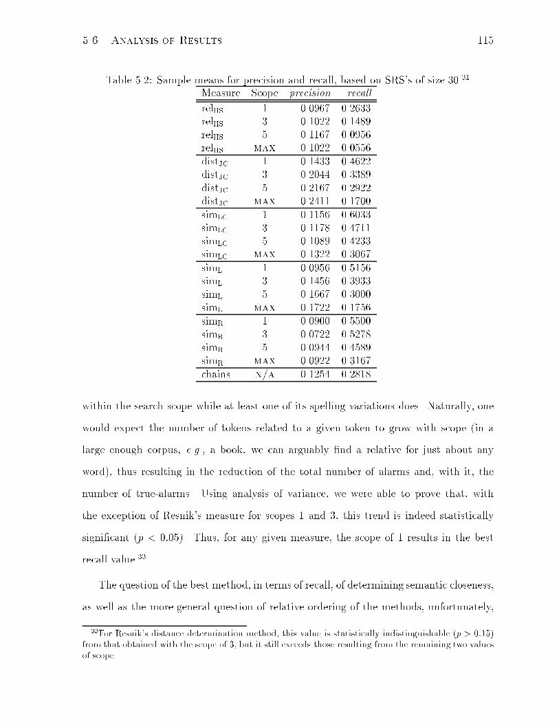
5.6. Analysis of Results 115
Table 5.2: Sample means for precision and recall, based on SRS's of size 30.31
Measure Scope precision recall
relHS 1 0.0967 0.2633relHS 3 0.1022 0.1489relHS 5 0.1167 0.0956relHS max 0.1022 0.0556distJC 1 0.1433 0.4622distJC 3 0.2044 0.3389distJC 5 0.2167 0.2922distJC max 0.2411 0.1700simLC 1 0.1156 0.6033simLC 3 0.1178 0.4711simLC 5 0.1089 0.4233simLC max 0.1322 0.3067simL 1 0.0956 0.5156simL 3 0.1456 0.3933simL 5 0.1667 0.3000simL max 0.1722 0.1756simR 1 0.0900 0.5500simR 3 0.0722 0.5278simR 5 0.0944 0.4589simR max 0.0922 0.3167chains n/a 0.1254 0.2818
within the search scope while at least one of its spelling variations does. Naturally, one
would expect the number of tokens related to a given token to grow with scope (in a
large enough corpus, e.g., a book, we can arguably �nd a relative for just about any
word), thus resulting in the reduction of the total number of alarms and, with it, the
number of true-alarms. Using analysis of variance, we were able to prove that, with
the exception of Resnik's measure for scopes 1 and 3, this trend is indeed statistically
signi�cant (p < 0:05). Thus, for any given measure, the scope of 1 results in the best
recall value.33
The question of the best method, in terms of recall, of determining semantic closeness,
as well as the more general question of relative ordering of the methods, unfortunately,
33For Resnik's distance determination method, this value is statistically indistinguishable (p > 0:15)from that obtained with the scope of 3, but it still exceeds those resulting from the remaining two valuesof scope.
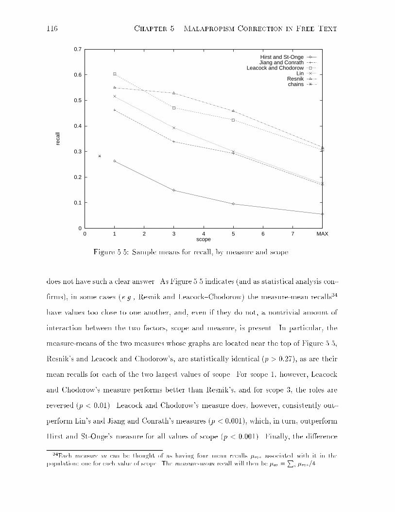
116 Chapter 5. Malapropism Correction in Free Text
0
0.1
0.2
0.3
0.4
0.5
0.6
0.7
0 1 2 3 4 5 6 7 MAX
reca
ll
scope
Hirst and St-OngeJiang and Conrath
Leacock and ChodorowLin
Resnikchains
Figure 5.5: Sample means for recall, by measure and scope.
does not have such a clear answer. As Figure 5.5 indicates (and as statistical analysis con-
�rms), in some cases (e.g., Resnik and Leacock{Chodorow) the measure-mean recalls34
have values too close to one another, and, even if they do not, a nontrivial amount of
interaction between the two factors, scope and measure, is present. In particular, the
measure-means of the two measures whose graphs are located near the top of Figure 5.5,
Resnik's and Leacock and Chodorow's, are statistically identical (p > 0:27), as are their
mean recalls for each of the two largest values of scope. For scope 1, however, Leacock
and Chodorow's measure performs better than Resnik's, and for scope 3, the roles are
reversed (p < 0:01). Leacock and Chodorow's measure does, however, consistently out-
perform Lin's and Jiang and Conrath's measures (p < 0:001), which, in turn, outperform
Hirst and St-Onge's measure for all values of scope (p < 0:001). Finally, the di�erence
34Each measure m can be thought of as having four mean recalls �ms associated with it in thepopulation: one for each value of scope. The measure-mean recall will then be �m =
Ps �ms=4.
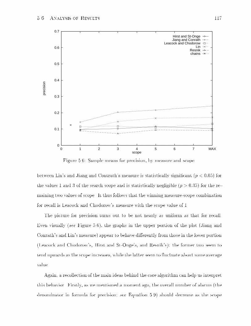
5.6. Analysis of Results 117
0
0.1
0.2
0.3
0.4
0.5
0.6
0.7
0 1 2 3 4 5 6 7 MAX
prec
isio
n
scope
Hirst and St-OngeJiang and Conrath
Leacock and ChodorowLin
Resnikchains
Figure 5.6: Sample means for precision, by measure and scope.
between Lin's and Jiang and Contrath's measure is statistically signi�cant (p < 0:05) for
the values 1 and 3 of the search scope and is statistically negligible (p > 0:35) for the re-
maining two values of scope. It thus follows that the winning measure-scope combination
for recall is Leacock and Chodorow's measure with the scope value of 1.
The picture for precision turns out to be not nearly as uniform as that for recall.
Even visually (see Figure 5.6), the graphs in the upper portion of the plot (Jiang and
Conrath's and Lin's measure) appear to behave di�erently from those in the lower portion
(Leacock and Chodorow's, Hirst and St-Onge's, and Resnik's): the former two seem to
tend upwards as the scope increases, while the latter seem to uctuate about some average
value.
Again, a recollection of the main ideas behind the core algorithm can help us interpret
this behavior. Firstly, as we mentioned a moment ago, the overall number of alarms (the
denominator in formula for precision; see Equation 5.9) should decrease as the scope
118 Chapter 5. Malapropism Correction in Free Text
increases, due to the fact that fewer tokens will be agged as potential malapropisms.
On the other hand, once a token has been identi�ed as a potential malapropism, it has
a higher chance of resulting in an alarm, and a true-alarm in particular, the larger the
scope, for its (intended) spelling correction is more likely to turn out to have related
tokens.
Statistical analysis reveals that, for Leacock and Chodorow's, Hirst and St-Onge's,
and Resnik's measure, the search scope does not constitute a statistically signi�cant
factor (i.e., their graphs are actually at). The main qualitative di�erence between
these measures and the Jiang{Conrath and Lin is the fact that, for the latter two, the
variation in precision is signi�cant (p < 0:001) for the values 1 and 3 of the scope (after
which, however, the graphs also level o�). Overall, scope 3 can therefore be considered
as resulting in the best value of precision.
Analyses of variance and contrasts show that Jiang and Conrath's measure performs
best in terms of precision. Lin's measure comes second with its precision mean for
scope 1 being statistically indistinguishable (p > 0:19) from those of the remaining three
measures, but the precision means corresponding to scope 3 (and larger) exceeding theirs.
Finally, the measure-means of Leacock and Chodorow's and Hirst and St-Onge's measures
are statistically indistinguishable (marginally, p = 0:067), but both exceed the mean of
Resnik's measure. From these observations, we can conclude that Jiang and Conrath's
measure with the search scope of 3 delivers the highest mean precision.
Lastly, we address the question of the best overall performance, i.e., optimum recall
and precision. Note that the superiority of smaller values of scope for recall and the
statistical insigni�cance of larger values of scope for precision narrow the discussion
to the scope sizes of 1 and 3. In fact, for the Leacock{Chodorow and Hirst{St-Onge
measures, the scope size of 1 is the unique choice. For Resnik's measure, we can also pick
scope 3 | and obtain statistically equivalent performance. Since the precision values for
scope 1 of all the three measures are statistically indiscernible, the relative ranking of
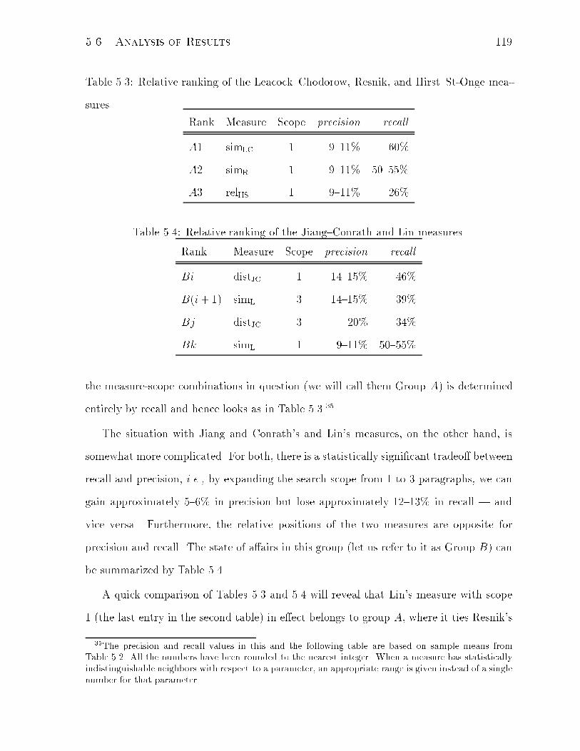
5.6. Analysis of Results 119
Table 5.3: Relative ranking of the Leacock{Chodorow, Resnik, and Hirst{St-Onge mea-
sures.
Rank Measure Scope precision recall
A1 simLC 1 9{11% 60%
A2 simR 1 9{11% 50{55%
A3 relHS 1 9{11% 26%
Table 5.4: Relative ranking of the Jiang{Conrath and Lin measures.
Rank Measure Scope precision recall
Bi distJC 1 14{15% 46%
B(i+ 1) simL 3 14{15% 39%
Bj distJC 3 20% 34%
Bk simL 1 9{11% 50{55%
the measure-scope combinations in question (we will call them Group A) is determined
entirely by recall and hence looks as in Table 5.3.35
The situation with Jiang and Conrath's and Lin's measures, on the other hand, is
somewhat more complicated. For both, there is a statistically signi�cant tradeo� between
recall and precision, i.e., by expanding the search scope from 1 to 3 paragraphs, we can
gain approximately 5{6% in precision but lose approximately 12{13% in recall | and
vice versa. Furthermore, the relative positions of the two measures are opposite for
precision and recall. The state of a�airs in this group (let us refer to it as Group B) can
be summarized by Table 5.4.
A quick comparison of Tables 5.3 and 5.4 will reveal that Lin's measure with scope
1 (the last entry in the second table) in e�ect belongs to group A, where it ties Resnik's
35The precision and recall values in this and the following table are based on sample means fromTable 5.2. All the numbers have been rounded to the nearest integer. When a measure has statisticallyindistinguishable neighbors with respect to a parameter, an appropriate range is given instead of a singlenumber for that parameter.
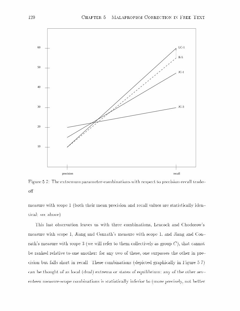
120 Chapter 5. Malapropism Correction in Free Text
10
20
40
50
60
30
precision recall
LC-1
R-5
JC-1
JC-3
Figure 5.7: The extremumparameter-combinations with respect to precision-recall trade-
o�.
measure with scope 1 (both their mean precision and recall values are statistically iden-
tical; see above).
This last observation leaves us with three combinations, Leacock and Chodorow's
measure with scope 1, Jiang and Conrath's measure with scope 1, and Jiang and Con-
rath's measure with scope 3 (we will refer to them collectively as group C), that cannot
be ranked relative to one another: for any two of these, one surpasses the other in pre-
cision but falls short in recall. These combinations (depicted graphically in Figure 5.7)
can be thought of as local (dual) extrema or states of equilibrium: any of the other sev-
enteen measure-scope combinations is statistically inferior to (more precisely, not better
5.6. Analysis of Results 121
than) one of these three (e.g., Resnik's measure with scope 5 yields statistically the same
precision but poorer recall than Leacock and Chodorow's with scope 1; see Figure 5.7),
and an attempt at a maximum improvement of one performance criterion of a member
of group C (e.g., recall of Jiang and Conrath's with scope 1) with a minimum sacri�ce
in the other criterion (precision) will result in adopting another member of the group
(Leacock and Chodorow's with scope 1; note that we cannot adopt Resnik's with scope
5, because if we did, the gain in recall would not be maximal).
Hence, from the user's perspective, Leacock and Chodorow's measure with the search
scope of 1 should be used if recall is at a premium; Jiang and Conrath's measure with the
scope of 3 should be used if the highest possible (mean) precision is desired; �nally, Jiang
and Conrath's measure with scope 1 should be used for an optimummidway performance.

122 Chapter 5. Malapropism Correction in Free Text
Chapter 6
Conclusion
6.1 Measuring Semantic Relatedness
6.1.1 Summary
Evaluating the degree of semantic proximity between a pair of lexically expressed concepts
is a problem with a long history in philosophy, psychology, and arti�cial intelligence,
which pervades much of computational linguistics, and many di�erent perspectives on
which have been proposed.
The objective of this work has been to take stock of some computational methods of
measuring semantic relatedness that have appeared within the last decade or so, along
with their applications, o�er some insights into the question of their relative comparison,
and, �nally, suggest directions for future research in the area.
To this end, we have presented a survey of 13 approaches, classifying them by the
principal knowledge-source they deploy. These have included dictionary- and thesaurus-
based approaches, approaches using a semantic network (such as MeSH or WordNet), as
well as approaches combining multiple knowledge sources (in particular, a knowledge-rich
source such as a thesaurus and a knowledge-poor source such as corpus statistics).
A variety of recently developed applications of measures of semantic relatedness have
123
124 Chapter 6. Conclusion
also been presented, from resolution of word-sense ambiguity to discourse segmentation
to word prediction in speech and text recognition.
Given the diversity and the sheer number of existing ways to gauge semantic relat-
edness, the question of their (comparative) assessment naturally arises. While human
relatedness-ratings of concept pairs should, by de�nition, be regarded as the standard
against which ratings produced by computational measures are to be evaluated, obtain-
ing a sizeable set of reliable, subject-independent judgements proves highly problematic.
As a result, all of the attempts to perform an evaluation of this sort that we are aware
of [Resnik, 1995, Jiang and Conrath, 1997, Lin, 1998] have been based on a set of no
more than 30 pairs [Miller and Charles, 1991]. For the sake of compatibility and research
continuity, we followed up on these attempts, extending the evaluation to more measures
and a larger set of 65 pairs [Rubenstein and Goodenough, 1965]. For our main evaluation,
however, we opted to perform a comparison within the framework of a particular NLP
application.
We selected six proposals, all using WordNet as their (semantic) knowledge source,
of which we were able to successfully (re)implement �ve: Hirst and St-Onge's, Jiang and
Conrath's, Leacock and Chodorow's, Lin's, and Resnik's, thus representing simple-path-
length, scaled-path-length, and hybrid semantic-network approaches. These �ve measures
then participated in a word-pair relatedness rating exercise, the principal quantitative
outcome of which was coe�cients of correlation with human ratings, as well as in a
malapropism-correction experiment (see below).
6.1.2 Conclusions and Future Directions
The �gures of correlation with human judgements do not conclusively point to the su-
periority of any one particular method. In fact, our �ndings seem to refute or, at least,
weaken some of the previous claims. We should, however, reiterate our assertion that
even 65 pairs constitute too small a test set to be taken too seriously. Our �rst suggestion
6.1. Measuring Semantic Relatedness 125
for future work then pertains more to research in psycholinguistics than in computational
linguistics: larger collections of human ratings need to be compiled and cognitive pro-
cesses involved in making relatedness judgements by humans need to be further studied.
As will be discussed in more detail in the following section, our test NLP-application
was a system for detecting and correcting malapropisms. Deviating from the previous
practice [St-Onge, 1995, Hirst and St-Onge, 1998], we have focused on precision and
recall as its performance indicators. No measure, or measure-scope combination, has been
found optimal in terms of both of these simultaneously (e.g., distJC excels in precision,
while simLC and simR deliver best recall). We have, however, shown the question of
relative ranking to have a parsimonious solution, with twenty combinations reduced to
three optimal.
Despite being a step forward, the current evaluation scheme still allows us to draw
only limited inferences concerning the `goodness' of the measures of semantic relatedness
plugged into the system. For instance, Resnik's good recall and poor precision suggest
that the reason for the former is merely a large total number of generated alarms. Un-
fortunately, this by itself does not tell us much about the behavior of the measure, e.g.,
whether it `overrelates' or `underrelates' (since, for a word to result in an alarm, the word
must be declared unrelated to its context, while its spelling variation must be found to
have a relative). Thus, our second suggestion for future research is to develop other
performance-assessment methodologies for the malapropism detection task that would
be more `transparent' with respect to the semantic distance measure used, and to seek
other NLP tasks that may inherently possess such transparency.
Of the �ve measures participating in our experiments, Hirst and St-Onge's was the
only one taking into account relationships other than is-a. As its creators suspected,
however, and as our �ndings con�rmed, its relative simplicity impairs its performance.
Nevertheless, our intuition dictates that relatedness measures of reasonable power should
yield better results in any tasks relying on context, and malapropism detection and cor-
126 Chapter 6. Conclusion
rection in particular, than measures of similarity alone. Hence, our next recommendation
is that e�orts be directed towards developing approaches that would exploit more fully
the gamut of semantic relationships already available in resources such as WordNet.1
These e�orts can build on some of the existing research [St-Onge, 1995, Sussna, 1997,
Jiang and Conrath, 1997], which has suggested, for instance, that local network density,
depth of a node, strength of a link, and link type and direction should be among the
factors to be given consideration. A possible �rst step in this direction may be to at-
tempt transplanting measures de�ned on the is-a hierarchy to other hierarchies, such as
part-of and the verb is-a hierarchy.
In fact, we can go one step further and remove the restriction of being semantic from
the set of relations we propose to be considered.2 That is, even from our preliminary
investigation, it is safe to say that the future belongs to hybrid methods.
An important milestone in improving the quality of computational assessment of
semantic relatedness should be identi�cation and incorporation of additional sources of
linguistic knowledge such as domain-speci�c thesauri, statistical word usage information,
etc. [Morris and Hirst, 1991], as well as merging of those already in active use. In addition
to the initiatives of Resnik, Lin, and Jiang and Conrath, we should mention recent work
by Tokunaga et al. [1997] and Fujii et al. [1997]. Carrying out this program will also
help alleviate the problem of part-of-speech restrictions presently imposed on a number
of measures by their principal knowledge sources.
Incidentally, the paradigm of merging can probably also be applied to measures them-
selves. That is, we could form a new measure relNew by combining several existing ones
1The emphasis on is-a in the current research is less surprising if we realize that the relationship isthe cornerstone of any dictionary that follows Aristotelian principles: is-a is the relationship that holdsbetween a headword and its genus [Guthrie et al., 1996]. However, it is the other relations that makedi�erentia possible.
2The distinction between semantic and non-semantic has not been �rmly established. Kozima andFurugori [1993], for instance, speak of paradigmatic relations (\how the words are associated with eachother") and syntagmatic relations (\how the words are arranged in sequential texts"). Our use ofterminology is similar, although we would like to include unary statistical relationships, such as corpusfrequency, etc., in the non-semantic category.
6.1. Measuring Semantic Relatedness 127
relOld1; : : : ; relOldN. As a general case, our new measure can be viewed as returning a vec-
tor whose components correspond to the relatedness values of its constituent measures.
How such vectors are manipulated, i.e., the precise manner in which the constituent
measures are combined, might vary (and might even ultimately depend on an applica-
tion): to determine whether the pair c1; c2 is more closely related than c3; c4, we could
compare the norms of relNew(c1; c2) and relNew(c3; c4), or simply see whether a majority
of relNew(c1; c2)'s coordinates have larger values than their relNew(c3; c4)'s counterparts
(essentially letting the component measures relOld1; : : : ; relOldN `vote'; cf Leacock and
Chodorow's simultaneous use of two measures, Section 4.1.3, page 53), or adopt another
strategy.
A related issue is whether measures of semantic relatedness or distance should be
quantitative (i.e., returning a numerical expression indicative of the strength of related-
ness) or qualitative (i.e., giving a, say, binary response, such as related/unrelated). We
do insist that measures returning a numerical value are more useful than those merely
giving a binary response. First, it is feasible to go from the former to the latter, as
we have demonstrated in Section 5.4.2, but not vice versa. Second, many applications
can make e�ective use of numerical expressions of distance (to see, for instance, which
of a number of concepts is closest to a given one; cf ranking of candidate corrections
discussed in the next section). Lastly, as we saw in Chapter 3, a range of values should
allow for a more comprehensive assessment of measures.
Finally, recall that this report has zeroed in on measures of semantic relatedness be-
tween the most elementary units: lexemes. However, a fair amount of work, most notably
in the �elds of Information Retrieval and Extraction, has been devoted to determining
relatedness between larger textual units: phrases, sentences, or even entire texts. In a
typical IR approach (e.g., the vector space model [Salton, 1989], \one of the most suc-
cessful approaches" according to Green [1997b]), a text (document) is represented by a
vector whose elements correspond to the terms used in the text and are indicative of
128 Chapter 6. Conclusion
the term's relative frequency; the (semantic) distance between a pair of texts is then
computed geometrically. There thus appears to exist a considerable gap between lexeme-
relatedness measures, as discussed in this report, and commonly used text-relatedness
measures: while the latter do indeed start with lexemes, lexical equivalence, instead of
lexical semantic relatedness, is used at the lexeme level | and an altogether di�erent
methodology is used to go from there to the text level.
The e�orts of Green (Section 4.3.2), Rada and colleagues (Section 4.5.1), and Richard-
son and Smeaton (Section 4.5.2) are examples of attempts to bridge this gap. However,
they address only the �rst problem above. What we would also like to see is methods
of computing relatedness between texts that more closely parallel (or extend) methods
of computing relatedness between words (perhaps, by virtue of both being derived from
the same general principle). We hence propose that in the design of future measures of
semantic relatedness between lexemes, consideration should be given to the question of
their extensibility to larger textual units. Of the work known to us, perhaps that of Lin
[1997a] and Jiang [1998] a�ord precedents, but the task overall remains a challenge.
6.2 Detection and Correction of Malapropisms
6.2.1 Summary
Although originally conceived primarily as a framework for application-speci�c evaluation
(see previous section), our excursion into detecting and correcting malapropisms grad-
ually developed into a project in its own right. Following up on the work of Hirst and
St-Onge [1998], we introduced a su�cient number of modi�cations to their algorithm and
implementation for the new malapropism corrector described in Chapter 5 to be regarded
as a distinct system.
The new system still relies on Hirst's principle that if a word appears out of context
and is a plausible mistyping for another word that �ts into the context, it is likely to be a
6.2. Detection and Correction of Malapropisms 129
malapropism. Unlike its predecessor, however, our system avoids the overhead associated
with persistent segmentation of context. Instead, the context is viewed merely as a bag
of words (whose size is a parameter of execution; see below). Verifying whether a word
�ts into its context then amounts to computing the word's semantic relatedness to every
other word in the bag and checking whether any of these exceed a threshold.
The adoption of this model motivated a number of other changes: bidirectional scan-
ning of context, paragraph-based context boundaries, partial, less committing, disam-
biguation, etc. Lower-level modi�cations included augmenting the system with a proper-
name recognition engine, addressing the issue of morphological ambiguity, and improving
the strategy for replacement-candidate generation.
We evaluated the performance of our malapropism detection and correction system
with �ve di�erent plug-in measures of semantic distance (see Section 6.1) and four dif-
ferent sizes of context, or search scope3: 1, 3, or 5 paragraphs surrounding a target word,
and the entire text. For each of the 20 combinations, the program was run on a set
of 481 Wall Street Jounal articles, in which one in roughly every 200 words had been
replaced with a malapropism (and which were large enough to warrant at least one such
replacement).
6.2.2 Conclusions and Future Directions
As we reported in Section 6.1.2, no single measure-scope combination has been found
to deliver simultaneously the best precision and recall. Of the twenty combinations,
however, our system outperformed St-Onge's [1995] in terms of precision for seven, in
terms of recall for 14, and in terms of both for six.4
A couple of interesting observations have beenmade about the e�ect of the context size
3Here `search' refers to the search for related words, which is performed only inside a context.4Unfortunately, we cannot provide any statistical support for these comparisons, for, whereas our
precision and recall �gures are actually means obtained through random sampling of output, St-Onge'sare but overall proportions.
130 Chapter 6. Conclusion
on the system performance. Although intuition suggests that precision should increase
and recall should decrease as the size of context increases, only the latter tendency
has turned out to be statistically signi�cant for the measures that took part in our
experiments (with a minor exception; refer to Section 5.6.3 for details): the di�erence
in precision was substantial only for the context sizes of 1 and 3 paragraphs and only
for two out of the �ve measures. Thus, our �ndings point towards overall optimality of
smaller scopes.
It should be reiterated here that the search methodology employed in St-Onge's [1995]
original system di�ered from ours. In particular, the search scope was measured in
sentences and varied according to the type of connection sought (e.g., the entire text
for the extra-strong, �7 sentences for the strong, and �3 for the medium-strong). In
order to keep the framework for all of the measures in our experiments uniform, this
custom-tailored scheme had to be replaced. As a result, the performance �gures for our
system using Hirst and St-Onge's measure appear5 lower than those of St-Onge's system.
Hence, while we believe that our view of context is both more principled and universally
applicable, additional investigation may be in order.
Another algorithm parameter that may require further work is the relatedness thresh-
old (Section 5.4.2). While, by virtue of the design of Hirst and St-Onge's measure, this
was not an issue in their system, when adapting the other four measures to use in our
task, we had to select a point in their ranges that would mark the boundary between the
related and the unrelated. This was done by examining the rankings of Rubenstein and
Goodenough's pairs produced by the measures in our experiment of Chapter 3 against
those of human judges and against each other. As we have mentioned, however, the relia-
bility of inductions made on the basis of this dataset may be questionable due to its size.
Thus, we propose that alternative ways of deriving thresholds be explored, such as using
pairs from the same thesaural category [Lin, 1997b] or even brute-force experimentation
5See footnote 4, page 129
6.2. Detection and Correction of Malapropisms 131
with various values of thresholds as a system parameter.
This work has demonstrated the overall signi�cance of the measure parameter in
our algorithm. All of the representatives of the class of hybrid measures that we have
worked with (and for whose superiority we have argued in Section 6.1.2), on the other
hand, have an additional subparameter: the corpus for deriving concept frequencies.
Thus, when using such measures as plug-ins, varying the frequency corpus according to
the text submitted for malapropism correction, e.g., obtaining genre-speci�c frequency
counts | from a proofread newswire corpus for a newspaper article, from an edited novel
for a story, etc. | may be another way to improve performance.
Because of the central role of the relatedness computations in our system, most lim-
itations that a given measure of relatedness possesses are `inherited' by the system. An
example of such a limitation is the part-of-speech restriction: as we mentioned in Sec-
tion 6.1.2, all of the measures that we have worked with are de�ned on nominal concepts
only. To mitigate the severity of this restriction somewhat, we decided to treat as a noun
anything that looks like one, either as is or after stemming. For instance, the adjective
drunk in drunk driver will be taken to be a noun; likewise, the verb drank will be trans-
formed into drink, which, again, is present in the noun lexicon and so will be considered
a noun in searches for relatives. While the �rst example appears quite reasonable, many
will argue that drinking is a better nominalization of drank than drink is. A more so-
phisticated nominalization mechanism (paired, for instance, with the alternative-lemma
facility; see Section 5.3.3.4) may also become a performance-improving factor.
The handling of compound words is yet another avenue for investigation and possible
improvement. As reported in Section 5.3.3.3, our simple-minded attempt to extend the
special treatment of multiword compounds (con�rmation by default) to the single-word
case mis�red: along with network and stockbroker, terms like thousand and relationship
were identi�ed as compounds. Incorporating the knowledge of common su�xes, such as
-ship, as well as modifying the con�rmation strategy (for instance, to con�rm only those
132 Chapter 6. Conclusion
compounds one or more of whose components have relatives, e.g., henhouse since hen is
related to fox occurring nearby) may constitute a good starting point.
Kukich [1992] partitions the task of word-error correction into three subtasks: \(1)
detection of an error; (2) generation of candidate corrections; and (3) rank-
ing of candidate corrections". Due to our system's role as a testbed in relatedness
experiments, in this work we ended up focusing on malapropism detection. It is there-
fore worth emphasizing here that the system has been designed also with a view to
malapropism correction. Recall (Section 5.3.2) that a crucial step in deciding whether
a potential malapropism is a malapropism indeed is coming up with its spelling varia-
tions that would �t into the context. This automatically takes care of the second step
in Kukich's breakdown. One can then imagine that, during an interactive session, the
list of all such spelling variations (candidate replacements) can be o�ered to the user,
perhaps even without the need for ranking. In the setting of fully-automatic spelling cor-
rection, on the other hand, choosing the best candidate, to be substituted into the text,
is essential. At present, this is an open chapter in our implementation. A strategy that
meshes most naturally with the existing algorithm is to rank the candidates according to
their proximity to the context: e.g., the relatedness value with the context word closest
semantically or physically. In our preliminary experiments, the intended correction was
found among the candidate replacements for about 78{97% of the detected malapropisms
(approximately 83%, 92%, and 96% for the three optimal measure-scope combinations).
However, no `best-�rst' statistics have been collected so far. Addressing issues more-
immediately related to the corrective capacity of our system should prove to be another
interesting direction for future research.
Appendix A
Sample Text With Introduced
Malapropisms
Below is the text of one of the 481 Wall Street Journal articles,1 (automatically) altered
to include four malapropisms, that were submitted to our malapropism corrector. The
malapropisms are italicized and their intended corrections (i.e., the words appearing in
the text originally) are given immediately next to them in square brackets.
A.1 Text
Charles T. Russell used to play trombone in Pittsburgh burlesque houses and with big
bands in the Southeast. He gave it up for banking, but he still knows how to attract a
crowd.
Mr. Russell, the president of Visa International, a bank-owned credit-card association,
recently urged members to consider halting sales of American Express Co. services in
retaliation for the �nancial-service giant's recent decision to begin o�ering a new cut-
rate credit card.
1Copyright c 1987, 1988, 1989 Dow Jones Inc.; from Association for Computational Linguistics DataCollection Initiative CD-ROM 1 (September 1991)
133
134 Appendix A. Sample Text With Introduced Malapropisms
Consumer groups denounced the plea as an illegal restraint of trade, and Congress is
considering an inquiry. But Mr. Russell is resolute. \Banks need to realize that there is
a fox in the henhouse," he declares. Visa and the 56-year-old Mr. Russell, who enjoys
riding a Harley-Davidson motorcycle, have collided with consumers and Congress before.
Critics have long alleged that Visa member banks and other card issuers in ate interest
rates. As in past years, Congress is currently considering imposing rate ceilings, and some
consumer groups think such a law would be an appropriate response to Mr. Russell's
recent harangue.
But the push in Congress has fallen short in the past, with Mr. Russell's plain talk
helping to lead the apposition [opposition]. \He is more vociferous, but his statements
probably re ect the general thought of the leading card issuers," says Pete Hart, a First
Interstate Bancorp executive vice president.
Forewarned, First Interstate, which o�ers American Express Gold cards and travelers
checks, is \reevaluating our relationship" with American Express, according to Mr. Hart.
Nothing rash is planned, he says, but the new card | Optima | is \without question
an intrusion into our business."
American Express and the banks are used to being allies rather than adversaries.
American Express cards generally don't o�er revolving credit, and banks have marketed
them alongside their Visa and MasterCard cards, which do.
But Optima will compete head-on. The card will cost $15 a year, in addition to the
$45 that American Express charges for its regular card. But it will extend 13.5% credit.
The average Visa card also carries a $15 annual fee, but it has a sti�er 17.5% rate, and
several big banks charge even more.
American Express says only a limited number of existing customers will be o�ered
the new card. It doesn't expect to issue many more than two million of them by 1990,
compared with about 100 million current Visa card holders. It doesn't know what the
muss [fuss] is all about.
A.1. Text 135
\We are not basically in the credit business," says an American Express spokesman.
\We're going after a select market."
But the elite group that American Express is targeting has been a major source of
bank credit card earnings. Banks also believe that the American Express estimates are
too modest, and some fear a plastic rate war.
\They aren't going to fail," says Mr. Russell. \I don't admire their ethics, but I
certainly respect their knowledge." He thinks American Express is misleading consumers,
arguing that the Optima rate is closer to 18% when the tie-in with the regular card is
considered.
The ap comes at a time when Visa and its members have few other reasons to
complain. There are 22% more Visa card holders world-wide than there were two years
ago. The group, which furnishes members with new products, system support and other
services, is developing computerized cards and new links with automated teller machines.
For the banks, credit cards have been a growing source of pro�ts, although tax changes
and a growing consumer debt load portend possibly slower future growth.
In orchestrating Visa's expansion, Mr. Russell has hit a few prong [wrong] notes with
bankers and competitors. Two years ago, he led the opposition against a merger proposal
from rival MasterCard, an idea that some bank issuers of both cards thought would cut
costs for them and consumers.
Mr. Russell says that the bene�ts were overrated and that a merger raises possible
antitrust problems. Instead, he has backed joint e�orts, but some question his interest
in cooperating. Visa and MasterCard have been studying a national network to process
retail store debit card transactions. Last fall, however, Visa agreed to manage a large
similar operation in California, and some MasterCard o�cials worried that the joint
venture had been doomed. Mr. Russell denies this.
His comments about American Express also have some precedent. Last summer, as
part of a campaign to blunt another budding competitor, Visa encouraged members to
136 Appendix A. Sample Text With Introduced Malapropisms
refuse to honor Sears, Roebuck & Co.'s Discover card in their automated teller machines.
Along the way, critics believe consumers have been cheated. Card rates haven't fallen
nearly as sharply as other interest rates since 1980. Current rates also re ect a jump
in write-o�s of bad credit card loans, which some banks have brought upon themselves
through aggressive marketing.
Mr. Russell argues that usury aw [law] depressed rates below market levels years
ago, making current rates seem high. He also says critics ignore administrative costs in
their rate attacks. The steeper write-o�s, he contends, stem more from \lax" bankruptcy
laws and heavy unemployment in the major oil-producing states than indiscriminate card
marketing.
While Mr. Russell faces possible congressional and Justice Department investigations
into his American Express comments, he says Visa welcomes the attention. \We've
nothing to hide, never had," adds the executive, who joined Visa in 1971.
Like scores of musicians, he put down his horn when television arrived in the 1950s.
While hunting for a music-store job one day in 1953, a rainstorm forced him to take cover
at a branch of what is now PNC Financial Corp. The bank hired him as a collector in its
installment loan department. He married a former Pittsburgh radio singer who he used
to back up in the band.
Weather permitting, Mr. Russell commutes every day from his Novato, Calif., home
in his single-engine airplane. The 20-minute ight helps him forget his troubles. \You
can't think about anything else when you're ying," he says. \When I y home, I don't
have a problem anymore."
Bibliography
[Agirre and Rigau, 1996] Eneko Agirre and German Rigau. Word sense disambiguation
using conceptual density. In Proceedings of the 16th International Conference on Com-
putational Linguistics (COLING-96), pages 16{22, Copenhagen, Denmark, August
1996.
[Agirre and Rigau, 1997] Eneko Agirre and German Rigau. A proposal for word sense
disambiguation using conceptual distance. In Ruslan Mitkov and Nicolas Nicolov,
editors, Recent Advances in Natural Language Processing: Selected Papers from
RANLP'95, volume 136 of Amsterdam Sudies in the Theory and History of Linguistic
Science: Current Issues in Linguistic Theory, chapter 2, pages 161{173. John Ben-
jamins Publishing Company, Amsterdam/Phildadelphia, 1997.
[Al-Halimi and Kazman, 1998] Reem Al-Halimi and Rick Kazman. Temporal indexing
through lexical chaining. In Christiane Fellbaum, editor, WordNet: An Electronic
Lexical Database, chapter 14, pages 333{352. The MIT Press, Cambridge, MA, 1998.
[Amsler, 1980] Robert A. Amsler. The structure of the Merriam-Webster Pocket Dictio-
nary. PhD thesis, University of Texas at Austin, December 1980.
[Atwell and Elliott, 1987] E. Atwell and S. Elliott. Dealing with ill-formed English text.
In R. Garside, G. Leach, and G. Sampson, editors, The Computational Analysis of
English: A Corpus-Based Approach, chapter 10. Longman, Inc., New York, 1987.
137
138 Bibliography
[Barzilay and Elhadad, 1997] Regina Barzilay and Michael Elhadad. Using lexical chains
for text summarization. In Proceedings of the ACL'97/EACL'97 Workshop on Intelli-
gent Scalable Text Summarization, pages 10{17, Madrid, Spain, July 1997.
[Brill, 1994] Eric Brill. Some advances in rule-based part of speech tagging. In Proceed-
ings of the Twelfth National Conference on Arti�cial Intelligence (AAAI-94), pages
256{261, Menlo Park, CA and Cambridge, MA, 1994. AAAI Press and MIT Press.
[Brooks et al., 1993] G. Brooks, T. Gorman, and L. Kendall. Spelling it out: the spelling
abilities of 11- and 15-year-olds. National Foundation for Educational Research, 1993.
[Cohen and Kjeldsen, 1987] Paul R. Cohen and Rick Kjeldsen. Information retrieval by
constrained spreading activation in semantic networks. Information Processing and
Management, 23(4):255{268, 1987.
[Collins and Loftus, 1975] Allan M. Collins and Elizabeth F. Loftus. A spreading-
activation theory of semantic processing. Psychological Review, 82(6):407{428, Novem-
ber 1975.
[Evens, 1988] Martha Walton Evens, editor. Relational models of the lexicon: represent-
ing knowledge in semantic networks, chapter 1. Studies in Natural Language Process-
ing. Cambridge University Press, 1988.
[Fellbaum, 1998] Christiane Fellbaum, editor. WordNet: An Electronic Lexical Database.
The MIT Press, Cambridge, MA, 1998.
[Flexner, 1983] S. B. Flexner, editor. Random House Unabridged Dictionary. Random
House, New York, second edition, 1983.
[Francis and Ku�cera, 1982] Winthrop Nelson Francis and Henry Ku�cera. Frequency
Analysis of English Usage: Lexicon and Grammar. Houghton Mi�in, Boston, 1982.
Bibliography 139
[Fujii et al., 1997] Atsushi Fujii, Toshihiro Hasegawa, Takenoby Tokunaga, and Hozumi
Tanaka. Integration of hand-crafted and statistical resources in measuring word sim-
ilarity. In Proceedings of the ACL'97/EACL'97 Workshop on Automatic Information
Extraction and Building of Lexical Semantic Resources for NLP Applications, Madrid,
Spain, July 1997.
[Golding and Roth, 1996] Andrew R. Golding and Dan Roth. Applying Winnow to
context-sensitive spelling correction. In Lorenza Saitta, editor, Machine Learning:
Proceedings of the 13th International Conference, pages 182{190, Bari, Italy, 1996.
Morgan Kaufmann (San Fransisco, CA).
[Golding and Schabes, 1996] Andrew R. Golding and Yves Schabes. Combining trigram-
based and feature-based methods for context-sensitive spelling correction. In Proceed-
ings of the 34th Annual Meeting of the Association for Computational Linguistics,
pages 71{78, Santa Cruz, CA, 1996.
[Golding, 1995] Andrew R. Golding. A Bayesian hybrid method for context-sensitive
spelling correction. In Proceedings of the Third Workshop on Very Large Corpora,
pages 39{53, Boston, MA, 1995.
[Green, 1997a] Stephen J. Green. Building hypertext links in newspaper articles using
semantic similarity. In Proceedings of the Third Workshop on Applications of Natu-
ral Language to Information Systems (NLDB'97), pages 178{190, Vancouver, British
Columbia, June 1997.
[Green, 1997b] Stephen Joseph Green. Automatically Generating Hypertext by Comput-
ing Semantic Similarity. PhD thesis, University of Toronto, 1997.
[Grosz and Sidner, 1986] Barbara Grosz and Candance Sidner. Attention, intentions and
the structure of discourse. Computational Linguistics, 12(3):175{204, 1986.
140 Bibliography
[Guthrie et al., 1996] Louise Guthrie, James Pustejovsky, Yorick Wilks, and Brian M.
Slator. The role of lexicons in natural language processing. Communications of the
ACM, 39(1):63{72, January 1996.
[Harman, 1994] Donna Harman. Overview of the third Text Retrieval Conference
(TREC-3). In Proceedings of the third Text Retrieval Conference, November 1994.
[Hearst, 1994] Marti A. Hearst. Multi-paragraph segmentation of expository text. In
Proceedings of the 32nd Annual Meeting of the Association for Computational Lin-
guistics, pages 9{16, Las Cruces, New Mexico, June 1994.
[Hirst, 1987] Graeme Hirst. Semantic Interpretation and the Resolution of Ambiguity.
Studies in Natural Language Processing. Cambridge University Press, 1987.
[Hirst and St-Onge, 1998] Graeme Hirst and David St-Onge. Lexical chains as repre-
sentations of context for the detection and correction of malapropisms. In Christiane
Fellbaum, editor, WordNet: An Electronic Lexical Database, chapter 13, pages 305{
332. The MIT Press, Cambridge, MA, 1998.
[Jiang and Conrath, 1997] Jay J. Jiang and David W. Conrath. Semantic similarity
based on corpus statistics and lexical taxonomy. In Proceedings of International Con-
ference on Research in Computational Linguistics (ROCLING X), Taiwan, 1997.
[Jiang, 1998] Jian (Jay) Jiang. Lexical Semantic Similarity and Its Application to Busi-
ness Catalog Retrieval. PhD thesis, University of Waterloo, Canada, 1998.
[Kazman et al., 1995] Rick Kazman, WilliamHunt, and Marilyn Mantei. Dynamic meet-
ing annotation and indexing. In Proceedings of the 1995 Paci�c Workshop on Dis-
tributed Meetings, pages 11{18, Honolulu, HI, March 1995.
Bibliography 141
[Kazman et al., 1996] Rick Kazman, Reem Al-Halimi, William Hunt, and Marilyn Man-
tei. Four paradigms for indexing video conferences. IEEE MultiMedia, 1996. Spring
1996.
[Kominek and Kazman, 1997] John Kominek and Rick Kazman. Accessing multimedia
through concept clustering. In Proceedings of CHI97 Conference on Human Factors
in Computing Systems, pages 19{26, Atlanta, Georgia, March 1997. ACM SIGCHI,
ACM.
[Kozima and Furugori, 1993] Hideki Kozima and Teiji Furugori. Similarity between
words computed by spreading activation on an English dictionary. In Proceedings
of 6th Conference of the European Chapter of the Association for Computational Lin-
guistics (EACL-93), pages 232{239, Utrecht, 1993.
[Kozima and Ito, 1997] Hideki Kozima and Akira Ito. Context-sensitive [measurement
of] word distance by adaptive scaling of a semantic space. In Ruslan Mitkov and
Nicolas Nicolov, editors, Recent Advances in Natural Language Processing: Selected
Papers from RANLP'95, volume 136 of Amsterdam Sudies in the Theory and History
of Linguistic Science: Current Issues in Linguistic Theory, chapter 2, pages 111{124.
John Benjamins Publishing Company, Amsterdam/Phildadelphia, 1997.
[Kukich, 1992] Karen Kukich. Techniques for automatically correcting words in text.
Computing Surveys, 24(4):377{439, 1992.
[Leacock and Chodorow, 1998] Claudia Leacock and Martin Chodorow. Combining local
context and WordNet similarity for word sense identi�cation. In Christiane Fellbaum,
editor,WordNet: An Electronic Lexical Database, chapter 11, pages 265{283. The MIT
Press, Cambridge, MA, 1998.
142 Bibliography
[Lee et al., 1993] Joon Ho Lee, Myong Ho Kim, and Yoon Joon Lee. Information re-
trieval based on conceptual distance in IS-A hierarchies. Journal of Documentation,
49(2):188{207, June 1993.
[Lin, 1997a] Dekang Lin. An information-theoretic de�nition of similarity. Submitted to
`Computational Intelligence', 1997.
[Lin, 1997b] Dekang Lin. Using syntactic dependency as local context to resolve word
sense ambiguity. In Proceedings of ACL/EACL-97, pages 64{71, Madrid, Spain, July
1997.
[Lin, 1998] Dekang Lin. An information-theoretic de�nition of similarity. In Proceedings
of International Conference on Machine Learning, Madison, Wisconsin, July 1998.
[Luhn, 1968] Hans Peter Luhn. The automatic creation of literature abstracts. In
Claire K. Schultz, editor, H. P. Luhn: Pioneer of Information Science. Spartan Books,
New York, 1968.
[McGill et al., 1979] M. McGill et al. An evaluation of factors a�ecting document rank-
ing by information retrieval systems. Project report, Syracuse University School of
Information Studies, 1979.
[McKeown and Radev, 1995] Kathleen McKeown and Dragomir Radev. Generating
summaries of multiple news articles. In Proceedings of SIGIR-95, 1995.
[Miller and Charles, 1991] George A. Miller and Walter G. Charles. Contextual corre-
lates of semantic similarity. Language and Cognitive Processes, 6(1):1{28, 1991.
[Miller et al., 1990] George A. Miller, Richard Beckwith, Christiane Fellbaum, Derek
Gross, and Katherine Miller. Five papers on WordNet. CSL Report 43, Princeton
University, 1990. revised August 1993.
Bibliography 143
[Miller et al., 1993] George A. Miller, Claudia Leacock, Randee Tengi, and R. T. Bunker.
A semantic concordance. In Proceedings of the ARPA Human Language Technology
Workshop, pages 303{308, San Fransisco, 1993. Mogan Kaufman.
[Miller, 1998] George A. Miller. Nouns in WordNet. In Christiane Fellbaum, editor,
WordNet: An Electronic Lexical Database, chapter 1, pages 23{46. The MIT Press,
Cambridge, MA, 1998.
[Mitton, 1987] Roger Mitton. Spelling checkers, spelling correctors, and the misspellings
of poor spellers. Information Processing Management, 23(5):495{505, 1987.
[Mitton, 1996] Roger Mitton. English Spelling and the Computer. Studies in language
and linguistics. Longman Group Limited, 1996.
[Morris, 1988] Jane Morris. Lexical cohesion, the thesaurus, and the structure of text.
Master's thesis, University of Toronto, December 1988. Published as Technical Report
CSRI-219.
[Morris and Hirst, 1991] Jane Morris and Graeme Hirst. Lexical cohesion computed by
thesaural relations as an indicator of the structure of text. Computational Linguistics,
17(1):21{48, March 1991.
[Okumura and Honda, 1994] Manabu Okumura and Takeo Honda. Word sense disam-
biguation and text segmentation based on lexical cohesion. In Proceedings of the
Fifteenth International Conference on Computational Linguistics (COLING-94), vol-
ume 2, pages 755{761, Kyoto, Japan, August 1994.
[Osgood, 1952] C. E. Osgood. The nature and measurement of meaning. Psychological
Bulletin, 49:197{237, 1952.
[Passonneau and Litman, 1993] Rebecca J. Passonneau and Diane J. Litman. Intention-
based segmentation: Human reliability and correlation with linguistic cues. In Pro-
144 Bibliography
ceedings of the 31st Annual Meeting of the Association for Computational Linguistics,
pages 148{155, 1993.
[Pollock and Zamora, 1983] J. J. Pollock and A. Zamora. Collection and characterization
of spelling errors in scienti�c and scholarly text. Journal of the American Society for
Information Science, 34(1):51{58, 1983.
[Quillian, 1968] M. Ross Quillian. Semantic memory. In M. Minsky, editor, Semantic
Information Processing. MIT Press, Cambridge, MA, 1968.
[Rada and Bicknell, 1989] Roy Rada and Ellen Bicknell. Ranking documents with a
thesaurus. JASIS, 40(5):304{310, September 1989.
[Rada et al., 1989] Roy Rada, Hafedh Mili, Ellen Bicknell, and Maria Blettner. Devel-
opment and application of a metric on semantic nets. IEEE Transactions on Systems,
Man, and Cybernetics, 19(1):17{30, February 1989.
[Resnik, 1995] Philip Resnik. Using information content to evaluate semantic similarity.
In Proceedings of the 14th International Joint Conference on Arti�cial Intelligence,
pages 448{453, Montreal, Canada, August 1995.
[Richardson and Smeaton, 1995a] Ray Richardson and Allan F. Smeaton. Automatic
word sense disambiguation in a KBIR application. Working paper CA-0595, School of
Computer Applications, Dublin City University, 1995.
[Richardson and Smeaton, 1995b] Ray Richardson and Allan F. Smeaton. Using Word-
Net in a knowledge-based approach to information retrieval. Working paper CA-0395,
School of Computer Applications, Dublin City University, 1995.
[Rubenstein and Goodenough, 1965] Herbert Rubenstein and John B. Goodenough.
Contextual correlates of synonymy. Communications of the ACM, 8(10):627{633, Oc-
tober 1965.
Bibliography 145
[Salton, 1989] Gerard Salton. Automatic text processing. Addison-Wesley, 1989.
[Sparck Jones, 1993] Karen Sparck Jones. What might be in a summary? In Gerhard
Knorz, J�urgen Krause, and Christa Womser-Hacker, editors, Information Retrieval
'93: Von der Modellierung zur Anwendung, Proceedings der 1. Tagung Information Re-
trieval '93, pages 9{26. Universit�at Regensburg, Universit�atsverlag Konstanz, Septem-
ber 1993.
[St-Onge, 1995] David St-Onge. Detecting and correcting malapropisms with lexical
chains. Master's thesis, University of Toronto, March 1995. Published as Technical
Report CSRI-319.
[Sterling, 1983] C. M. Sterling. Spelling errors in context. British Journal of Psychology,
74:353{364, 1983.
[Sussna, 1993] Michael Sussna. Word sense disambiguation for free-text indexing using
a massive semantic network. In Proceedings of the Second International Conference
on Information and Knowledge Management (CIKM-93), pages 67{74, Arlington, Vir-
ginia, 1993.
[Sussna, 1997] Michael John Sussna. Text Retrieval Using Inference in Semantic
Metanetworks. PhD thesis, University of California, San Diego, 1997.
[Tokunaga et al., 1997] Takenobu Tokunaga, Atsushi Fujii, Makoto Iwayama, Naoyuki
Sakurai, and Hozumi Tanaka. Extending a thesaurus by classifying words. In Proceed-
ings of the ACL'97/EACL'97 Workshop on Automatic Information Extraction and
Building of Lexical Semantic Resources for NLP Applications, Madrid, Spain, July
1997.
[Wei, 1993] Mei Wei. An analysis of word relatedness correlation measures. Master's
thesis, University of Western Ontario, London, Ontario, May 1993.
146 Bibliography
[West, 1953] Michael Philip West. A general service list of English words, with seman-
tic frequencies and a supplementary word-list for the writing of popular science and
technology. Longman, Harlow, Sussex, 1953.
[Wing and Baddeley, 1980] A. M.Wing and A. D. Baddeley. Spelling errors in handwrit-
ing: a corpus and a distributional analysis. In Uta Frith, editor, Cognitive Processes
in Spelling, pages 251{85. Academic Press, 1980.
[Witten et al., 1994] Ian H. Witten, Alistair Mo�at, and Timothy C. Bell. Managing
Gigabytes: Compressing and indexing documents and images. Van Nostrand Reinhold,
1994.
[Wu and Palmer, 1994] Zhibiao Wu and Martha Palmer. Verb semantics and lexical
selection. In Proceedings of the 32nd Annual Meeting of the Association for Computa-
tional Linguistics, pages 133{138, Las Cruces, New Mexico, June 1994.