TIPPING AND RESIDENTIAL SEGREGATION: A UNIFIED …JOURNAL OF REGIONAL SCIENCE, VOL. 51, NO. 1, 2011, pp. 167–193 TIPPING AND RESIDENTIAL SEGREGATION: A UNIFIED SCHELLING MODEL* Junfu

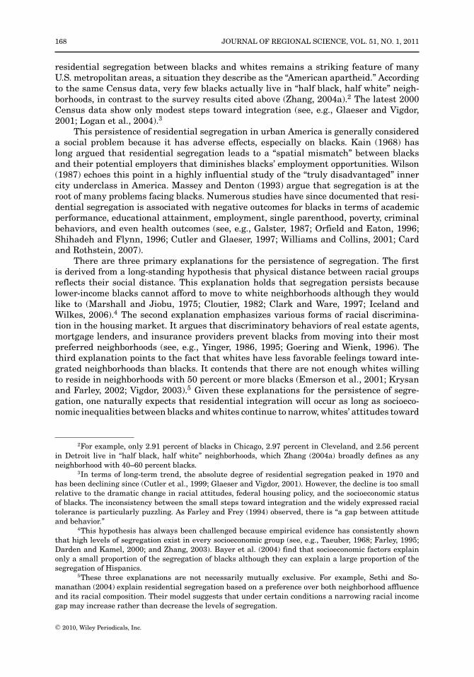
JOURNAL OF REGIONAL SCIENCE, VOL. 51, NO. 1, 2011, pp. 167–193

TIPPING AND RESIDENTIAL SEGREGATION: A UNIFIEDSCHELLING MODEL*

Junfu ZhangDepartment of Economics, Clark University, 950 Main Street, Worcester, MA 01610.E-mail: [email protected]

ABSTRACT. This paper presents a Schelling-type checkerboard model of residential segregation for-mulated as a spatial game. It shows that although every agent prefers to live in a mixed-race neighbor-hood, complete segregation is observed almost all of the time. A concept of tipping is rigorously defined,which is crucial for understanding the dynamics of segregation. Complete segregation emerges andpersists in the checkerboard model precisely because tipping is less likely to occur to such residentialpatterns. Agent-based simulations are used to illustrate how an integrated residential area is tippedinto complete segregation and why this process is irreversible. This model incorporates insights fromSchelling’s two classical models of segregation (the checkerboard model and the neighborhood tippingmodel) and puts them on a rigorous footing. It helps us better understand the persistence of residentialsegregation in urban America.

1. INTRODUCTION

For three decades, survey data have consistently shown that African Americansprefer to live in integrated neighborhoods with half blacks or a slight black majority.1

For example, in 1982, the General Social Surveys asked black respondents about theirmost preferred neighborhood racial composition and found that 61.6 percent of thempicked “half black, half white” as the top choice (Davis and Smith, 1993). Data collectedin a Multi-City Study of Urban Inequality (MCSUI) during the 1990s also showed that50 percent of black interviewees chose a 50–50 neighborhood as the most attractive and99 percent of them indicated a willingness to move into such neighborhoods (Krysan andFarley, 2002).

Survey results also demonstrated that whites, although generally less enthusiasticabout 50–50 type neighborhoods than blacks, have increasingly endorsed the idea ofresidential integration (Schuman et al., 1997). The same MCSUI data indicated that60 percent of whites felt comfortable with neighborhoods with one-third blacks and that45 percent of whites were willing to move into such neighborhoods (Charles, 2003).

These stated preferences are in stark contrast with the high levels of racial housingsegregation in reality. Using the 1990 Census data, Massey and Denton (1993) find that

*This paper has benefited from comments by Alex Anas, Richard Arnott, Robert Axtell, MarlonBoarnet (editor), Robert Helsley, Amy Ickowitz, Robert McMillan, Juan Robalino, Steve Ross, Harris Selod,Peyton Young, three anonymous referees, and seminar or conference participants at Boston College, ClarkUniversity, Northeastern University, SHUFE, WPI, the ESHIA Conference at George Mason University,the Econometric Society Summer Meetings at Duke, the Workshop on Residential Sprawl and Segregationin Dijon, France, the Third World Congress of the Game Theory Society at Northwestern University, andthe ASSA Meetings in San Francisco.

Received: May 2008; revised: April 2009; accepted: August 2009.1See, for example, Farley et al. (1978), Farley et al. (1994), Farley et al. (1997), Krysan and Farley

(2002), Schuman et al. (1997), and Bobo and Zubrinsky (1996).

C© 2010, Wiley Periodicals, Inc. DOI: 10.1111/j.1467-9787.2010.00671.x

167

168 JOURNAL OF REGIONAL SCIENCE, VOL. 51, NO. 1, 2011

residential segregation between blacks and whites remains a striking feature of manyU.S. metropolitan areas, a situation they describe as the “American apartheid.” Accordingto the same Census data, very few blacks actually live in “half black, half white” neigh-borhoods, in contrast to the survey results cited above (Zhang, 2004a).2 The latest 2000Census data show only modest steps toward integration (see, e.g., Glaeser and Vigdor,2001; Logan et al., 2004).3

This persistence of residential segregation in urban America is generally considereda social problem because it has adverse effects, especially on blacks. Kain (1968) haslong argued that residential segregation leads to a “spatial mismatch” between blacksand their potential employers that diminishes blacks’ employment opportunities. Wilson(1987) echoes this point in a highly influential study of the “truly disadvantaged” innercity underclass in America. Massey and Denton (1993) argue that segregation is at theroot of many problems facing blacks. Numerous studies have since documented that resi-dential segregation is associated with negative outcomes for blacks in terms of academicperformance, educational attainment, employment, single parenthood, poverty, criminalbehaviors, and even health outcomes (see, e.g., Galster, 1987; Orfield and Eaton, 1996;Shihadeh and Flynn, 1996; Cutler and Glaeser, 1997; Williams and Collins, 2001; Cardand Rothstein, 2007).

There are three primary explanations for the persistence of segregation. The firstis derived from a long-standing hypothesis that physical distance between racial groupsreflects their social distance. This explanation holds that segregation persists becauselower-income blacks cannot afford to move to white neighborhoods although they wouldlike to (Marshall and Jiobu, 1975; Cloutier, 1982; Clark and Ware, 1997; Iceland andWilkes, 2006).4 The second explanation emphasizes various forms of racial discrimina-tion in the housing market. It argues that discriminatory behaviors of real estate agents,mortgage lenders, and insurance providers prevent blacks from moving into their mostpreferred neighborhoods (see, e.g., Yinger, 1986, 1995; Goering and Wienk, 1996). Thethird explanation points to the fact that whites have less favorable feelings toward inte-grated neighborhoods than blacks. It contends that there are not enough whites willingto reside in neighborhoods with 50 percent or more blacks (Emerson et al., 2001; Krysanand Farley, 2002; Vigdor, 2003).5 Given these explanations for the persistence of segre-gation, one naturally expects that residential integration will occur as long as socioeco-nomic inequalities between blacks and whites continue to narrow, whites’ attitudes toward

2For example, only 2.91 percent of blacks in Chicago, 2.97 percent in Cleveland, and 2.56 percentin Detroit live in “half black, half white” neighborhoods, which Zhang (2004a) broadly defines as anyneighborhood with 40–60 percent blacks.

3In terms of long-term trend, the absolute degree of residential segregation peaked in 1970 andhas been declining since (Cutler et al., 1999; Glaeser and Vigdor, 2001). However, the decline is too smallrelative to the dramatic change in racial attitudes, federal housing policy, and the socioeconomic statusof blacks. The inconsistency between the small steps toward integration and the widely expressed racialtolerance is particularly puzzling. As Farley and Frey (1994) observed, there is “a gap between attitudeand behavior.”

4This hypothesis has always been challenged because empirical evidence has consistently shownthat high levels of segregation exist in every socioeconomic group (see, e.g., Taeuber, 1968; Farley, 1995;Darden and Kamel, 2000; and Zhang, 2003). Bayer et al. (2004) find that socioeconomic factors explainonly a small proportion of the segregation of blacks although they can explain a large proportion of thesegregation of Hispanics.

5These three explanations are not necessarily mutually exclusive. For example, Sethi and So-manathan (2004) explain residential segregation based on a preference over both neighborhood affluenceand its racial composition. Their model suggests that under certain conditions a narrowing racial incomegap may increase rather than decrease the levels of segregation.

C© 2010, Wiley Periodicals, Inc.

ZHANG: TIPPING AND RESIDENTIAL SEGREGATION 169

integrated neighborhoods continue to become more favorable, and antidiscrimination lawsare more stringently enforced.6

In this paper, I show that the prospect of residential integration may be bleakerthan what is generally perceived. I present a rigorous model that incorporates importantinsights from Thomas Schelling’s two models of segregation (Schelling, 1969, 1971, 1972,and 1978). I will show that residential segregation could emerge and persist even if thefollowing three conditions hold simultaneously: (1) There exists no racial discriminationof any type; (2) both blacks and whites prefer to live in 50–50 neighborhoods; and (3) thesocioeconomic disparities between blacks and whites are completely eliminated.

This paper makes two contributions. First, it offers an explanation for the persistenceof residential segregation in U.S. metropolitan areas observed in the past two decades.Existing studies on the persistence of segregation generally assume that if integrationis a preferred outcome, then segregation could persist only if some frictions prevent thetransition to integration. This is why many researchers consider racial discrimination andincome disparities as possible reasons for the persistence of segregation (Dawkins, 2004).Deviating from this literature, this paper emphasizes that racial integration, even if highlydesirable at the individual level, may not be attainable because integrated residentialpatterns are inherently unstable. This idea is well known because of Schelling’s pioneeringstudies and follow-up work, but it has not been a focus of recent research on the persistenceof segregation.

Second, this paper formalizes Schelling’s idea of tipping and uses it to rigorouslydemonstrate why residential segregation may emerge and persist despite the preferencefor integration at the individual level. Schelling originally developed the idea of tippingto study segregation dynamics in a single neighborhood and the concept has always beendiscussed in the context of a single neighborhood. Schelling also showed, in a multi-neighborhood setting, that residential patterns may not reflect individual preferences. Byintroducing the idea of tipping into a multineighborhood model, this paper incorporatesthe insights from Schelling’s separate models into a unified framework. Unlike Schelling’sinductive and less formal approach, this paper presents a rigorous model and analyzesit using techniques from mathematical game theory, which helps sharpen many of theimportant insights developed by Schelling.

The remainder of the paper is organized as follows. Section 2 reviews Schelling’stwo dynamic models of segregation. Section 3 presents a unified Schelling model thatcombines the insights from both of his models. Section 4 uses agent-based simulationsto illustrate the analytical results of the unified model. Section 5 concludes with someremarks.

2. SCHELLING’S MODELS OF SEGREGATION

In a series of publications, Schelling (1969, 1971, 1972, and 1978) presents two dis-tinct models of residential segregation between blacks and whites: the spatial proximitymodel and the bounded-neighborhood model.7 Each model provides great insights into

6In fact, there is evidence for the changing attitudes of whites. Survey data show that more andmore whites tend to agree with the principle that blacks should be able to live wherever they can affordand that more and more whites tend to approve open-housing laws (Schuman et al., 1997; Bobo, 2001).Time-series data from the Detroit area also show that whites are more and more willing to remain in theirneighborhoods as blacks enter (Farley et al., 1994). This change in attitudes alone could lead to a declinein racial discrimination. Ross and Turner (2005) find that indeed discriminatory behaviors have becomeless pervasive in U.S. housing markets.

7Schelling (1972) focuses on the bounded-neighborhood model only and calls it the “neighborhoodtipping” model. Each of the other works covers both models.



the causes and the persistence of racial housing segregation. Both are well known andhighly influential among social scientists far beyond the research area of segregation.

The spatial proximity model is a simulation of the dynamics of segregation. It startswith a residential area (a line or a grid) populated by a fixed number of black and whiteagents, each having a preference over the racial composition of her immediate neighbor-hood. Agents dissatisfied with their current residential locations are allowed to move intotheir preferred neighborhoods in a random order. The simulation stops when no agent isfound to be discontent. Schelling’s most striking finding is that moderate preferences forsame-color neighbors at the individual level can be amplified into complete residentialsegregation at the macro level. For example, if every agent requires at least half of herneighbors to be of the same color—a preference far from extreme—the final outcome,after a series of moves, is almost always complete segregation. Thus Schelling concludedthat the “macrobehavior” in a society may not reflect the “micromotives” of its individualmembers.

The spatial proximity model has every ingredient of a great theoretical work: itaddresses an important real world issue; it is simple to understand; it produces unex-pected results; and it has deep implications for various social sciences. In addition, themodel also has the appealing feature that any reader can come up with a variation ofits two-dimensional version and simulate it, for example, by moving dimes and pennieson a checkerboard. This model has since become widely known as Schelling’s “checker-board model.” Because of this work, many researchers today consider Schelling to be apioneer in agent-based computational economics (Epstein and Axtell, 1996, p. 3). Themodel’s numerous variations and the robustness of its main result have been a popu-lar topic in the area of agent-based modeling (see, e.g., Epstein and Axtell, 1996; Bruchand Mare, 2006; Fossett, 2006; Fagiolo et al., 2007; Pancs and Vriend, 2007; O’Sullivan,2008).

Despite the important insight revealed in Schelling’s simulation of the checkerboardmodel, for many years social scientists were unable to rigorously analyze the model, pri-marily because of the lack of suitable mathematical tools. Young (1998) was the first topoint out that techniques recently developed in evolutionary game theory—particularlythe concept of stochastic stability introduced by Foster and Young (1990)—are useful foranalyzing Schelling’s spatial proximity model. Young (1998, 2001) presents a simple vari-ation of the one-dimensional Schelling model (on a ring). He shows that segregation tendsto appear in the long run even though a segregated neighborhood is not preferred by anyagent.8 Pancs and Vriend (2007) derive similar results showing that complete segregationis the only possible long-run outcome on a ring when agents with a preference for 50–50neighborhoods play best response to neighborhood racial composition.9 Formulating thecheckerboard model as a spatial game played on a two-dimensional lattice graph, Zhang(2004a) shows that even if everybody prefers to live in a 50–50 mixed-race neighborhood,complete segregation emerges and persists in the long run under fairly general conditions.All of these results are even stronger than those Schelling showed in his original model.In another paper, Zhang (2004b) enriches the checkerboard model by adding a simplehousing market. It not only offers an alternative account of residential segregation, butalso produces testable hypotheses on housing price and vacancy differentials betweenpredominantly black and predominantly white neighborhoods. These studies all seek toreformulate Schelling’s checkerboard model in a game-theoretic framework and place it

8Bog (2006) assesses the robustness of the results from Young’s one-dimensional model.9This analytical result in Pancs and Vriend (2007) cannot be extended to a two-dimensional setting,

but using simulations they show that best-response dynamics tend to produce segregation even in atwo-dimensional space.



on a rigorous footing. The goal is to apply standard results in game theory to gain a betterunderstanding of the insights illustrated in Schelling’s checkerboard model.

Schelling’s second model of residential segregation, the “bounded-neighborhoodmodel,” is better known as the neighborhood tipping model.10 Unlike the checkerboardmodel, which is a simulation, the tipping model is purely analytical. It seeks to explainthe phenomenon of neighborhood tipping. Tipping is said to have occurred when an all-white neighborhood, after some blacks move in, suddenly begins the process of evolvinginto an all-black neighborhood with more and more whites moving out and only blacksmoving in. This process of tipping, once started, often appears to be accelerating andirreversible. Schelling’s explanation is based on the assumption that different residentsin a neighborhood have different tolerance levels toward the presence of neighbors of theopposite color. For example, in an all-white neighborhood, some residents may be will-ing to tolerate a maximum of 5 percent black neighbors; others may tolerate 10 percent,20 percent, and so on. The ones with the lowest tolerance level will move out if the pro-portion of black residents exceeds 5 percent. If only blacks move in to fill the vacanciesafter the whites move out, then the proportion of blacks in the neighborhood may reach alevel high enough to trigger the move-out of the next group of whites who are only slightlymore tolerant than the early movers. This process may continue and eventually result inan all-black neighborhood.

Similarly, an all-black neighborhood may be tipped into an all-white neighborhood,and a mixed-race neighborhood can be tipped into a highly segregated one, dependingon the tolerance levels of individuals in each racial group. In a more general sense, asSchelling points out, tipping refers to a process where “something disturbs the origi-nal equilibrium” (Schelling, 1971, p. 182). Most interestingly, this “something” may notbe “big” in any sense. It is sufficient to tip the system as long as it starts a chain re-action that moves the system further and further away from the original equilibriumsituation.11

The tipping model has also generated a great deal of interest. Some researchersadd a housing market into the model so that neighborhood choices are based on pricesinstead of preferences as in the original model (Schnare and MacRae, 1978; Becker andMurphy, 2000, Chapter 5). Others try to empirically detect the tipping phenomenon in thetransition of racial composition of neighborhoods (Goering, 1978; Clark, 1991; Easterly,2005; Card et al., 2008a, 2008b). In sociology, the tipping idea has been applied to studymany other social phenomena and inspired considerable theoretical work on “thresholdbehaviors” and critical mass models (see, e.g., Granovetter, 1978; Granovetter and Soong,1983, 1988; Crane, 1991). In economics, there has been some attempt to analyze thetipping phenomenon in a more rigorous setting. Anas (1980) proposes a formal model thatexplains neighborhood tipping on purely economic grounds without assuming prejudicial

10Schelling has two versions of the tipping model. The first version is most thoroughly analyzed ina section of Schelling (1971), in which he refers to it as the “bounded-neighborhood model.” A preview ofthis model appears in Schelling (1969) and an abridged version is included in Schelling (1978, Chapter 4).The second version of the tipping model is presented in Schelling (1972), focusing solely on the process ofneighborhood tipping. Schelling’s diagrammatic treatment of the neighborhood tipping process is slightlydifferent in these two versions of the model, although the central idea is the same.

11The concept of tipping has since been widely used by game theorists to refer to the idea that “a smallchange in the state of a system can cause a large jump in its equilibrium” (Heal and Kunreuther, 2006,p. 1). The tipping idea has even found its way into the popular culture. Most notably, in a national bestseller,Gladwell (2000) brilliantly explores and illustrates the tipping phenomenon using everyday examples. Hevery accurately summarizes the three characteristics of tipping dynamics as: (1) individual behaviorsare interdependent (contagious); (2) accumulation of small changes has significant consequences; and (3)dynamics accelerate once a threshold is reached (Gladwell, 2000, pp. 7–9).



preferences as Schelling did. Mobius (2000) and Dokumaci and Sandholm (2006) followSchelling more closely and seek to reformulate Schelling’s tipping model in a game-theoretic framework.12

One important aspect of Schelling’s original tipping model is that the events or activ-ities triggering the tipping process are assumed to be exogenous and thus not generatedwithin the model. In his own words, the initial in-migration of some blacks that tips anall-white neighborhood could be “concerted entry, erroneous entry by a few, organized in-troduction of a few, redefinition of the neighborhood boundary so that some who were notinside become ‘inside,’ or something of the sort” (Schelling, 1971, p. 182). Because tippingin this model has to be started by some outside events, Mobius (2000) argues that “thebasic tipping model suggests no mechanism for moving between an all-white equilibriumand a ghetto equilibrium. The theory can therefore explain the persistence but not theformation of ghettos.” He consequently extends the tipping model by introducing local in-teraction among residents within the neighborhood that gives an endogenous mechanismof tipping.

Schelling originally presented the checkerboard model and the tipping model inde-pendently. Aside from their common subject matter, they are related only in the sensethat both models help illustrate the deviation of macro behavior from micro motives.As already mentioned above, they have distinct formats: one as a simulation and theother as a purely analytical model. The key insight of the checkerboard model—moderatepreference for same-color neighbors may lead to complete segregation—is not shown inthe tipping model, and the concept of tipping—seemingly unimportant events trigger themovement of a system from one equilibrium to another—is not introduced in the checker-board model. The tipping model deals with a single neighborhood. It is thus a partialequilibrium model in that although agents (black or white) are assumed to move into andout of the neighborhood, the model does not specify where they come from or where theygo. In contrast, the checkerboard model consists of many neighborhoods and has a generalequilibrium flavor in that agents only move inside the model and their moves generateresidential segregation endogenously.13

These differences between Schelling’s checkerboard model and his tipping model havecaused research following these two models to develop along different paths that have notoverlapped. Similar to Schelling’s simulation with dimes and pennies on a checkerboard,the literature extending his checkerboard model is largely informal, using computer sim-ulation as the primary research tool. The main advantage of this approach lies in the easeof investigating any conceivable variations of the original model. As a consequence, thereare now many versions of the checkerboard model, most of which are more complicatedthan Schelling’s original model. However, the simulation approach also has its disad-vantages. Because different simulations are usually written in different programminglanguages and run on different platforms, simulation models are almost never directlybuilt on earlier work and therefore existing results are only loosely related. In addition,results derived from simulations are less transparent in that it is not always clear whichresult is driven by which assumptions. These problems can be overcome by developinga mathematical framework to rigorously analyze the checkerboard model. Young (1998)and Zhang (2004a, 2004b) are the early attempts in this direction. This paper is along thesame line of research.

12See also Bowles (2003, Chapter 2) for a variation of the bounded-neighborhood model that is usedto demonstrate the emergence of “spontaneous order.”

13The two models also have different neighborhood definitions. In the checkerboard model, neigh-borhoods are defined with reference to each agent’s residential location. The tipping model focuses on asingle neighborhood that has fixed boundaries; an agent is either inside it or outside it.



The literature inspired by Schelling’s tipping model has been more rigorous. A largefraction of the work in this tradition only borrows Schelling’s idea of tipping to studyother social phenomena rather than residential segregation. The studies that examinethe dynamics of segregation, like Schelling’s original tipping model, always focus on asingle neighborhood (e.g., Mobius 2000; Dokumaci and Sandholm 2006). However, segre-gation occurs at the city level and most of the features and consequences of residentialsegregation have to be understood at the city level. Therefore, in many cases, the multi-neighborhood setting of the checkerboard model is the more appropriate level of analysisthan the single-neighborhood setting of the tipping model. This paper represents the firstattempt to take the tipping idea developed in a single-neighborhood model and build itinto a checkerboard model that can be used to analyze segregation dynamics in a multi-neighborhood area.

I will present a Schelling-type checkerboard model that has the following features:First, it is formulated mathematically as a spatial game and thus can be rigorouslyanalyzed. Second, the concept of tipping is rigorously defined and the trigger of the tippingprocess is endogenized into the checkerboard model. Third, the tipping of equilibria iscrucial for understanding the dynamics of segregation in the checkerboard model. Fourth,the model helps us understand the persistence of segregation in U.S. metro areas.

3. A UNIFIED SCHELLING MODEL

Basic Setup

This model builds on a Schelling-type checkerboard model first proposed by Zhang(2004a). Zhang studies the model’s long-term dynamics, both analytically and compu-tationally, without introducing the concept of tipping. I will demonstrate here that thismodel can be extended to incorporate Schelling’s insights on neighborhood tipping. Tosimplify the analysis, I deviate from Schelling’s original setup by not leaving vacant lo-cations in the residential area. Following Young (1998), I allow individuals to move byswitching residential locations. It is as if there exists a centralized agency that processesall the information about who wants to move and which two agents may want to switch.

Consider an N × N lattice graph embedded on a torus, where N is an integer, asthe residential area of a city. There is a house at each vertex of the graph. Houses areidentical in every respect except that some are occupied by black agents and others bywhite agents. The proportion of blacks in the population is fixed and it has no bearing onthe results of the model. A neighborhood is defined locally in the way Schelling did. Inparticular, an agent takes 2n agents around her as her neighbors, where n is an integermuch smaller than N.

Each agent has a payoff function indicating how much she is willing to pay fora residential location in a particular neighborhood. The payoff function is specified asfollows:

�i = �u(si) + εi .(1)

An agent i’s payoff �i has two parts. The first part contains a deterministic term uthat denotes i’s utility derived from living in a particular neighborhood. This utilityis a function of si, the number of same-color neighbors agent i has. The second partεi is a random term. It is assumed to be independent both across agents and acrossresidential locations. Following the evolutionary game theory literature, one could think ofthis random term as a result of bounded rationality. For example, one may assume that theagent either does not have precise information about the neighborhood racial composition,or is incapable of correctly calculating her payoff, or act impulsively when deciding howmuch a residential location is worth. Alternatively, one could also interpret the random



FIGURE 1: An Agent’s Utility As a Function of Neighborhood Racial Composition.

term as a combination of nonracial characteristics of the neighborhood that residents careabout but are unobservable to the modeler. For example, such characteristics may includecrime rate, school quality, and proximity to workplace or natural amenities. For the easeof exposition, I will follow the bounded-rationality interpretation in the rest of the paperand analyze the model as if neighborhood racial composition is the only source of utility.However, it should be noted here that either interpretation gives the same set of results.

The parameter � in the payoff function is a positive constant that determines therelative importance of the random term. If � is close to zero, the random term is relativelyimportant and largely determines how much the agent is willing to pay for a particularresidential location. As a result, neighborhood racial composition plays a minor role whenan agent decides where to reside. If � approaches infinity, the random term becomesunimportant and only neighborhood racial composition matters in an agent’s decision.Throughout the paper, I consider the cases with a large �. It is assumed that every agenthas the same � and the same utility function u.

Assume that every agent prefers to live in an integrated neighborhood. More specifi-cally, every agent attains the highest level of utility when living in a half-black-half-whiteneighborhood. However, if such evenly mixed neighborhoods are not available, they feelbetter if they belong to the majority group rather than the minority group. That is, fora white agent, a 30–70 black-white ratio is better than a 70–30 black-white ratio; theopposite is true for a black agent. Survey data suggest that this is a plausible assump-tion. For example, a recent multicity study shows that individuals from all racial groupsprefer highly integrated neighborhoods, but at the same time they do have a bias in favorof own-group members (Charles, 2001, 2003; Krysan and Farley, 2002). Various reasonscould explain the inclination toward one’s own race, including cultural concerns, fear ofpotential hostility from the other group, or dislike of isolation.

To be more specific, I assume that an agent has a single-peaked utility function,depicted in Figure 1. Utility attains its maximum at n, which is half of the total numberof neighbors. On the left side of n, the function is linearly increasing; on the right side of n,it is linearly decreasing. It is relatively steeper on the left side, reflecting the assumptionthat agents would rather belong to the majority group instead of the minority group whenhalf-half mixed neighborhoods are unavailable. Linearity is assumed only for simplicity.



Letting si be the number of same-color neighbors agent i has, the utility function can bewritten as

u(si) =

⎧⎪⎪⎨⎪⎪⎩

Zsi

n, si ≤ n

(2Z − M) + (M − Z)si

n, si > n

Z > M > 0,(2)

where Z is the maximum value of u and M is the value of u when the agent has allneighbors like herself. Because the utility of having no same-color neighbors is normalizedto zero, M indicates the difference between living with all same-color neighbors and nosame-color neighbors.

Agents may exchange residential locations. In each period of time, a pair of agentsis randomly chosen from two different neighborhoods. The chosen agents are allowedto consider switching residential locations according to their own payoffs. Agents will al-ways trade residential locations when a switch is Pareto-improving (i.e., increases the twoagents’ total payoffs). In some cases, both agents have higher payoffs after a switch. Inother cases, a switch will lower one agent’s payoff, but it will be carried out as long as theother agent’s gain is enough to compensate the loss. I am therefore assuming that if nec-essary the two agents can always costlessly negotiate a proper side-payment to make thetrade mutually beneficial. This assumption allows me to focus on the sum of the two cho-sen agents’ payoffs because they always attempt to maximize the sum by a joint decision.

If the two agents choose to switch residential locations, the sum of their payoffs afterthe switch is

�i(· | switch) + � j(· | switch) = [�u(si | switch) + εi] + [�u(sj |switch) + ε j]

= �[u(si | switch) + u(sj | switch)] + [εi + ε j]

= �U + �,

where U = u(si|switch) + u(sj|switch) and � = εi + εj. Similarly, if the two agents do notswitch residential locations, the sum of their payoffs is

�i(· | not switch) + � j(· | not switch) = [�u(si | not switch) + ε′i] + [�u(sj | not switch) + ε′

j]= �[u(si | not switch) + u(sj | not switch)] + [ε′

i + ε′j]

= �V + �,

where V = u(si|not switch) + u(sj|not switch) and � = εi′ + εj

′.A switch will happen if and only if it yields higher total payoffs, that is, �U + �> �V +

�. Following McFadden (1973), I assume that � and � are independent and identicallyfollow an extreme value distribution. It is then well known that one can integrate out therandom terms of the total payoffs to obtain the probability of switching as

Pr(switch) = e�U

e�U + e�V.(3)

This switch rule is known as a log-linear behavioral rule, which is commonly assumedin the literature (see, e.g., Blume, 1997; Young, 1998; Brock and Durlauf, 2001). It impliesthat if a switch increases the agents’ utilities, they are more likely to do it. Note that evenif a switch decreases these two agents’ utilities, it is still possible that they will do it. Thepossibility of such a “mistake” depends on �.14 A large � implies that “mistakes” are rarely

14For expositional purpose, from this point on, I will refer to any move that lowers the two agents’utilities (derived from their racial preferences only) as a “mistake.” But note that a “mistake” does not haveto be a real mistake if one interprets the random term in an agent’s payoff function as random utilities.



made. In particular, as � approaches infinity, the probability of a switch approaches zeroif the switch results in lower utilities. In that case, the model reduces to a standard game-theoretic model with agents playing best reply to their environments. Random payoffs areunobservable. Thus, it is very convenient to integrate them out and analyze the model byworking with this behavioral rule.

Define a state x as an N2 vector, each element labeling a vertex of the N × Nlattice graph with the color of its occupant. Thus each x represents a specific residentialpattern. Let xt be the state at time t, which gives a finite Markov process under the switchrule described in Equation (3). Let P� denote the Markov process (i.e., its transitionprobability matrix). I call P� a perturbed process because agents do not always make“correct” (utility-increasing) decisions depending on the value of �. Small values of �imply large perturbations; the perturbation vanishes as � approaches infinity.

Let X be the set of all possible states of the Markov process. Given a large N, there area large number of states in X, implying a large number of possible residential patterns.To proceed, I will simplify the analysis by focusing on a single statistic of each residentialpattern specified as follows. Given any state, let ED be the set of all unordered black-whiteagent pairs who are neighbors

ED = {(i, j) | agents i and j are neighbors and have different colors}.A function � : X → N is then defined as the cardinality of the set ED: � = |ED|.

For any state xt, � (xt) gives the total number of pairs of unlike neighbors. In this model,the value of � (after being properly normalized) serves as a natural index of segregation.It measures the degree of exposure (or potential contact) between the members of the tworaces; it indicates the extent to which blacks and whites physically confront one anotherby virtue of sharing a common residential area. A lower � means a higher degree ofsegregation.15

The function � also has an attractive property; its first difference is proportional tothe changes in the moving agents’ utilities. This is summarized as the following lemma:16

LEMMA 1: For any two agents i and j in two different neighborhoods, the following relationalways holds:

� (· | switch) − � (· | not switch)

= −�{[u(si | switch) + u(sj | switch)] − [u(si | not switch) + u(sj | not switch)]},(4)

where � = 2n/M > 0 is a constant.

Equation (4) states that if two agents obtain higher utilities by switching residentiallocations, their action lowers the value of function � by an amount proportional to theincrease of their utilities. Following the game theory literature, from this point on, I willrefer to � as the potential function of the spatial game.17

Given that a smaller � implies a higher degree of segregation, Equation (4) suggeststhat utility-increasing switches will move the whole system toward segregation. In otherwords, a mutually beneficial trade of residential locations may have a negative effect onsocial welfare (sum of all agents’ utilities). The reason is that the switch of residential

15In empirical analysis, researchers have developed many indices to measure residential segrega-tion. See Massey and Denton (1988) for a detailed discussion.

16A sketch of the proof of this lemma is given by Zhang (2004a). A complete proof is included in anAppendix of the working paper version of this paper (Zhang, 2009), which is available upon request.

17Equation (4) makes this spatial game a potential game. A game is a potential game if the changesin players’ payoffs can be characterized by the first difference of a function. The function is then called thepotential function of the game (Monderer and Shapley, 1996).



FIGURE 2: Moore Neighborhood.

locations causes negative externalities. When agents move, they affect the racial compo-sition of both the neighborhoods they leave behind and the neighborhoods they move into.However, they do not take into account such externalities when they decide whether tomove. As it will become clear below, Equation (4) is crucial for analyzing the dynamics ofsegregation in this model.

Tipping

Consider the limiting situation of the Markov process P∞, that is, � = ∞. Rememberthat an infinitely large � implies that agents trade residential locations if and only if suchmoves increase their utilities (the deterministic terms of their total payoffs). I will referto this process as the unperturbed process because it is equivalent to setting the randomterm in an agent’s payoff function to be zero. Define an equilibrium state as one in whichthere does not exist a pair of agents who can increase their utilities by trading residentiallocations. An equilibrium is thus an absorbing state of the unperturbed process becauseonce the system is in it, it will never escape.

It is more convenient to discuss equilibrium states under a specific definition of aneighborhood. From now on, I use the definition of the “Moore neighborhood” in whichevery agent on the lattice graph considers the eight surrounding agents as neighbors(see Figure 2). Under this definition, a checkerboard residential pattern (each edge of thelattice graph connects a black agent with a white agent) is an equilibrium state. In thiscase, each agent has exactly four same-color neighbors out of a total of eight neighbors,which gives the highest possible utility level. Therefore, trading residential locations willnot increase any agent’s utility and no one has incentive to do it.

In addition to the checkerboard pattern, there exist a large number of equilibria (seeFigure 3). For example, a residential pattern with alternating black and white stripes isalso an equilibrium state. If a stripe consists of two rows of blacks or whites (panel (b) ofFigure 3), a typical agent has five same-color neighbors out of a total of eight. Clearly, noagent is living in a half-half mixed neighborhood and nobody attains the highest level ofutility. Nonetheless, it is impossible for any pair of agents to switch residential locationsto improve their utilities. The same is true if each stripe consists of more rows of blacksor whites (panel (c) of Figure 3). The most extreme case is a residential pattern in whichthere is only one stripe of blacks and one stripe of whites (panel (d) of Figure 3). In thiscase, one observes a complete segregation. But the system is still in equilibrium becauseno pair of agents can improve their situation by switching residential locations. Therefore,the system has multiple equilibria under the unperturbed process and different equilibriamay be associated with different levels of social welfare.

Now come back to the perturbed system that is subject to constant shocks in theform of utility-decreasing moves, that is, � is finite and large. Under this assump-tion, an equilibrium state as defined above is no longer an absorbing state. Althoughin an equilibrium state nobody gains utility by moving, there is still a (small) possi-bility that some agents will move, as implied by the behavioral rule in Equation (3).If agents indeed make such mistaken moves, the system is no longer in equilibrium



FIGURE 3: Equilibrium Residential Patterns.

because now some agents (including the ones that just moved) can improve their utili-ties by switching residential locations. It is possible that the agents that just moved willreverse their switch thus returning the system to its original equilibrium. However, itis also possible that some other agents will take moves and disturb the system furtheraway from its original equilibrium before it returns, especially now that some of suchmoves can be utility-improving because of the negative externalities created by otheragents’ mistaken moves earlier. In this way, an equilibrium state can be “tipped” awayby mistaken moves. The system will then evolve as agents move to increase (and, occa-sionally, mistakenly decrease) their utilities. At some point, it may reach an equilibriumstate that represents a residential pattern very different from the original equilibriumstate.



Value of ρ

a b cCommunicating states

FIGURE 4: Tipping between Two Equilibrium States in a Restricted Process.

I shall try to illustrate this process with a heuristic example depicted in Figure 4.Define two states as immediately communicating states if the system can travel from onestate to the other through a single switch of residential locations between two agents. Also,recall that each state corresponds to a value of the potential function � , the total numberof pairs of unlike neighbors. Consider a series of states lined up on the horizontal axis,each pair of adjacent states being two immediately communicating states. Assume thatthe value of the potential function at each state is given by the curve plotted in Figure 4.For the time being, assume that the system can only visit these states on the horizontalaxis. In particular, if the system is currently in state x (not an end point in Figure 4), onlytwo pairs of agents are allowed to consider a switch. If one pair is picked and they decideto switch residential locations, the system moves to the state on the left of x; if the otherpair is picked and they decide to switch, the system moves to the state on the right of x.In either case, if the picked agents do not switch, the system stays in state x.

The potential function shown in Figure 4 has two local minima at states a and c.Moving away from a or c, whether to the left or to the right, will increase the value offunction � and therefore by Equation (4) will decrease the moving agents’ utilities. Thusa and c are equilibrium states. Any other state is not an equilibrium because it alwayshas an adjacent state with a lower value of � , meaning that moving the system to thatadjacent state increases the total utilities of the agents who make the switch.

Consider the system that is restricted to the set of moves as shown in Figure 4.What will happen if the system happens to be in state a? It is very likely that it willstay there because moving in either direction increases the value of � and thus involvesutility-decreasing switches that occur with small probabilities. What if the system doesmove away from a as a result of a mistaken switch by two agents? It is then very likelythat the system will move back instead of moving further away from a, because movingback increases the agents’ utilities and moving further away does the opposite. In fact,starting from any state on the left side of b, it is most likely that the system would soonend up in a because it only takes a series of utility-improving moves. For the same reason,starting from any state on the right side of b, it is most likely that the system would



soon end up in the other equilibrium state c. Therefore, in the long run, the system wouldspend almost all the time in states a or c; a visit to any other state will necessarily betransient.

Now the question is whether the system tends to spend more time in a or in c. Again,suppose the system starts in state a. Notice that it takes a finite number of steps for thesystem to move to state b, each involving a utility-decreasing move that occurs with asmall probability. Given that each of these utility-decreasing moves can happen with apositive probability, there is a positive probability (although extremely small) that thiswhole series of mistaken moves occur one after another. In that case, the system will moveaway from a to the right and reach state b. If it goes beyond b, the system will likely moveto state c quickly because to do so only involves a series of utility-improving switches,each occurring with a probability close to one. Therefore, the system can be tipped awayfrom equilibrium state a through accumulation of mistaken moves and evolve into theother equilibrium c. Naturally, state b can be thought of as the tipping point because oncethis point is passed the system tends to quickly travel to c and the chance of returning toa is miniscule.

If the system can be tipped away from equilibrium state a, it can also be tippedaway from equilibrium state c. Tipping away from c will take a series of utility-decreasingswitches to move the system from c to b, after which it tends to quickly move toward abecause moving from b to a only involves utility-increasing switches. As shown in Figure 4,the potential function � attains different values at a and c. Its value at c is much smallerthan its value at a. This means that the increase in � as the system moves from a to bis much smaller than the increase in � as the system moves from c to b. In other words,moving the system from a to b requires fewer mistakes (or less serious mistakes measuredby the resulting utility losses) than moving the system from c to b. Thus, the probabilityof tipping away from a, although very small in absolute value, is many times larger thanthe probability of tipping away from c. Therefore, in the long run, the system would spendmost of the time in c or around c. The system does visit every state in the long run, butit will not be trapped in any of them because of the positive probability of making utility-decreasing switches. However, it is most difficult to escape from state c, not only moredifficult than from any of the nonequilibrium states, but also more difficult than from theother equilibrium state a.

Here is a quick summary of what I just demonstrated. In the simple example shownin Figure 4, there are two equilibrium states. Tipping could happen to either equilibriumthrough the accumulation of mistaken switches. However, the chance of tipping is muchsmaller for one equilibrium than the other, and therefore the equilibrium state that ismore resistant to tipping will naturally be observed most of the time in the long run.Interestingly, the equilibrium state more resistant to tipping is also the state that givesthe lowest value of the potential function. Recall that the potential function � is defined asthe total number of pairs of unlike neighbors. Thus the minimum value of � correspondsto the most segregated residential pattern.

In the analysis of the simplified example shown in Figure 4, the movement of thedynamical system is restricted to a small set of states. The unrestricted version of themodel is clearly much more complicated. Given a large dimension of the lattice graph, thetotal number of states (although finite) is very large; even the total number of equilibriumstates is fairly large. In addition, each state is directly communicating with a large numberof other states because a switch of residential locations between any black agent and anywhite agent will move the system to a different state. In the rest of this section, I will showthat the insight revealed by the simple example in Figure 4 is actually valid in general.

Consider any equilibrium state x. A large number of states differ from state x byonly one switch because any pair of agents may be chosen and make a switch. By the



definition of equilibrium, any state y directly communicating with x will never give thepotential function a lower value than x does. That is, the system can move from y to xthrough a utility-increasing (or utility-preserving) switch. Similarly, there may be somestates from which the system can travel to x by two or more switches, each of which eitherincreases or preserves the moving agents’ utilities. Define the basin of attraction of anequilibrium state x as the set of all states from which the system can travel to x through afinite number of steps that does not involve a single utility-decreasing switch. The statesthat belong to two basins of attraction can be thought of as the boundary between them.Starting from any equilibrium state, a series of utility-decreasing switches could movethe system away from the equilibrium and reach the boundary of its basin of attraction.Once the system passes the boundary, tipping has occurred because now the system is ina different basin of attraction and some utility-increasing (or utility-preserving) switcheswill take it to a different equilibrium.

Therefore, I formally define the tipping of an equilibrium as the process of moving outof its basin of attraction through the accumulation of low-probability utility-decreasingswitches. And a tipping point is a point on the boundary of the basin of attraction, beyondwhich the system can move further away from its original equilibrium with no utility-decreasing switches. Because tipping could happen to any equilibrium of the system, it isuseful to identify the ones that are more resistant to tipping than others.

To be intuitively appealing, an equilibrium state x that is resistant to tipping shouldhave the following two properties.

First, if the dynamical system is in state x, it has a high probability of remaining instate x in the next period. This implies that a mistaken switch will hardly ever happenwhen the system is in this equilibrium.

Second, if the dynamical system moves away from x as a result of one or a fewmistaken switches, there is a high probability of going back to x within a small number ofperiods. This implies that even if some mistaken switches have occurred, it takes manymore such utility-decreasing moves for the system to get out of the basin of attraction,thus it is likely to return to the original equilibrium before long.

If one thinks of “staying in x” as returning to x in one period of time, these two featuresare in fact the same: They both mean that the system, starting from the equilibrium statex, will return to x very soon. Therefore, it is sensible to measure an equilibrium state’sresistance to tipping using the expected number of periods for the system to return to theequilibrium given that it starts from the equilibrium.

Denoting r(x) as the resistance to tipping of equilibrium state x and P�xx(i) as the

probability of the system moving from state x to itself in exactly i periods, I define r(x) asthe following:

r(x) = 1∞∑

i=1

iP�xx(i)

.(5)

Given a finite �, P�xx(1)<1, implying that the sum in the denominator is larger than 1 and

therefore r(x) <1 for all x. Under this measure, an equilibrium state is considered moreresistant to tipping if it takes fewer periods (in expectation) for the system to return tothe equilibrium given that it starts there.

Main Result

I shall summarize the basic setup of the model as follows:(1) A finite number of black and white agents reside on a lattice graph, each occupy-

ing a vertex of the graph. (2) Each agent has a preference over the neighborhood racial



composition, which is represented by a single-peaked utility function in the form of Equa-tion (2) as shown in Figure 1. (3) In each period of time, two agents from different neigh-borhoods are randomly chosen and they decide on whether to switch residential locationsbased on the behavioral rule given by Equation (3).

Given these assumptions, one can prove the following theorem:

THEOREM: Given sufficiently large � and t, the residential pattern of complete segrega-tion is most resistant to tipping and is observed almost all the time.

I will give a sketch of the proof here. First, it is easy to check that the finite Markovchain defined in the model, P�, is irreducible, aperiodic, and recurrent. The process isirreducible because all states communicate with each other. It is aperiodic because startingin any state x, the system may enter state x again in any finite period of time. The processis recurrent because starting from any state x, the system will reenter state x in thefuture with probability one. It is a standard result in elementary Markov chain theorythat an irreducible, aperiodic, and recurrent Markov chain has a stationary distribution� such that �(x) is the probability of the system arriving in state x as time goes to infinity,independent of the initial state.18 �(x) can also be interpreted as the long-run proportionof time that the Markov chain is in state x. The following result links an equilibriumstate’s resistance to tipping to its stationary probability.19

LEMMA 2: Let r(x) be the resistance to tipping of state x and �(x) its stationary probability,then �(x) = r(x) for any state x.

Lemma 2 implies that if a state is more resistant to tipping, the dynamical systemspends a larger proportion of time in it in the long run. Given the definition of r(x), itmeans that the long-run proportion of time spent in state x equals the inverse of theexpected time between two consecutive visits to x.

To complete the proof of the theorem, I only need to show that �(x) decreases expo-nentially with � (x). This is given by the following lemma:20

LEMMA 3: If �(x) is the stationary distribution of the perturbed process P�, then

�(x) = e− ��

� (x)+c,(6)

where � > 0, � = 2n/M > 0, and c are all constants.

Recall that 2n is the size of a neighborhood and M is the utility loss of movingfrom a neighborhood with 100 percent same-color neighbors to a neighborhood with nosame-color neighbors. Given any two states x and y, it follows that

�(x)�(y)

= e− �M2n [� (x)−� (y)].(7)

Because �, M, and n are all positive, this ratio is greater than one if and only if� (y) > � (x). Let S be the set of all states that give a minimum � , that is, S = {x| � (x)≤ � (y) for all y in X}. Suppose x is a state in S and y is an arbitrary state such that � (y)> � (x). Given fixed values of M and n, the ratio �(x)/�(y) goes to infinity as � approachesinfinity. Therefore, if � is infinitely large, �(y) goes to zero for any y such that � (y) > � (x),and �(x) > 0 if and only if x is in S. In other words, only the states with a minimum � willhave a positive probability of being observed in the long run, and only these states have a

18See, for example, Taylor and Karlin (1998, p. 247) for a standard reference.19See the Appendix of Zhang (2009) for the proof of this lemma.20Again, see the Appendix in Zhang (2009) for the proof.



positive resistance to tipping: r(x) = �(x) > 0 if and only if x is in S. Because � is the totalnumber of unlike neighboring pairs, a state in S corresponds to complete segregation.Thus, in the long run, complete segregation exists almost all the time given sufficientlylarge �, which establishes the theorem.

Equation (7), derived from lemma 3, provides some useful insights into the forcesthat drive residential segregation. Consider any two states x and y such that � (x) < � (y),Equation (7) implies that the ratio �(x)/�(y) increases with � and M. That is to say, com-plete segregation (with minimum � ) is observed more often if � is larger and if M islarger. As discussed above, a large � means that the agents’ decision to switch residentiallocations is primarily determined by their preference over neighborhood racial composi-tion. A large M means that living with 100 percent same-color neighbors is much betterthan no same-color neighbors. Therefore, complete segregation in this model is driven bythe extent to which racial preference affects residential choice and the utility differencebetween living in an all-white neighborhood and living in an all-black neighborhood.

More interestingly, Equation (7) involves only M but not Z, the utility of living in ahalf-black-half-white neighborhood. That is, complete segregation emerges and persistsin this model entirely because living with all same-color neighbors is considered betterthan living with no same-color neighbors (M > 0). How much an agent likes the half-halfneighborhood (measured by the value of Z) is totally irrelevant. This is true because oncecomplete segregation emerges, mixed-race neighborhoods are rare and only exist alongthe color line. For most agents, the choice is between living with all white neighbors andliving with all black neighbors. It is thus natural that the difference between these twosituations determines the stability of segregation.

Equation (7) also makes it clear why it is necessary to assume a relatively smallneighborhood size 2n. Consider an extreme case in which 2n = N2 − 1, that is, an agentconsiders all other agents as her neighbors. Then, for any two states x and y, it is alwaystrue that � (x) = � (y) and thus �(x)/�(y) = 1. That is, any two states are observed with equalprobability even if � and M are large. Therefore, it is a necessary condition for segregationthat an agent only cares about the racial composition of nearby agents instead of the wholepopulation.

It is important to note that the analytical techniques developed in this section of thepaper are also applicable in other contexts. Consider again the states in S that minimizethe potential function � . Lemma 3 implies that

limt→∞,�→∞

�(x) > 0 if and only if x is in S.

This is precisely the defining property of a stochastically stable set in the game the-ory literature. Then the states in S are known as the stochastically stable statesor the stochastically stable equilibria of the spatial game (Foster and Young, 1990).Lemma 2, together with lemma 3, also implies that the states in S are the only states witha positive measure of resistance to tipping in limit. Therefore, in the process of provingthe theorem, I have demonstrated that the idea of tipping, as formulated here, is closelyrelated to the concept of stochastically stable equilibrium in evolutionary game theory. Infact, an equilibrium residential pattern’s property of being the most resistant to tippingwas shown to be equivalent to being stochastically stable. This theoretical insight thatlinks the intuitive concept of tipping to a broad set of analytical tools in mathematicalgame theory is likely to be useful for analyzing other types of tipping phenomena.

4. SIMULATION

This section presents agent-based simulations to illustrate the analytical resultsproved above. I arbitrarily choose a 30 × 30 lattice graph, so there are 900 agents in 900



residential locations. Again, the Moore neighborhood definition is used so that every agentconsiders the eight surrounding agents as neighbors. In all the simulations presentedbelow, I set � = 10.

I parameterize an agent’s utility function by setting n = 4, Z = 1, and M = 0.6.Equation (2) is thus reduced to the following mapping:

Number of same-color neighbors 0 1 2 3 4 5 6 7 8Utility 0 0.25 0.5 0.75 1 0.9 0.8 0.7 0.6

The first simulation starts from the residential pattern labeled as “stripes,” in whichtwo rows of blacks always follow two rows of whites (panel (a) in Figure 5).21 A typicalagent in this initial state has five same-color neighbors. Although this is not the mostpreferred situation from an agent’s point of view, the two groups are fairly integratedthroughout the area. As discussed above, this is an equilibrium state and only utility-decreasing switches can move the system out of the initial state.

Indeed, in a typical run of the simulation, the initial state stays unchanged forsome time after the simulation starts. However, this usually does not last long beforesome mistaken switches occur. And before such mistaken switches are reversed, someother mistaken ones follow. As panel (b) in Figure 5 shows, a series of utility-decreasingswitches have been made mistakenly, which has moved the system fairly far away fromits original equilibrium. In the initial state, the total number of unlike neighboring pairsis 1,260 (the value of “Rho” shown at the bottom of panel (a)). In panel (b), this numberhas increased to 1,359, as a result of all the mistaken switches. By now, the system is outof equilibrium and many pairs of agents can increase their utilities by trading residentiallocations if they are chosen to consider a switch. Such moves continue to happen overtime and the total number of unlike neighboring pairs continues to decline. As panel (c) ofFigure 5 shows, the whole area has evolved into a rather segregated residential pattern.In the long run, as shown in panel (d), complete segregation emerges. Every now andthen, mistaken moves still occur, which increases the value of � , but they only happenoccasionally and never push � back too high. Thus complete segregation persists overtime.

Figure 6 traces the evolution of � , which helps illustrate how tipping occurred tothe original equilibrium. For some time after the simulation starts, the value of � doesnot change. As mentioned above, this is because the starting state is an equilibrium andany switch in that situation will decrease utilities and thus will happen with a very smallprobability given a fairly large �. Eventually, such mistaken moves are taken and the valueof � increases. The accumulation of the mistaken moves soon pushes the system beyonda tipping point, which is shown as the � function reaches its maximum in Figure 6. Afterthat point, the � function declines rather sharply because many agents find that theycan increase their utilities by trading residential locations. However, each such switchactually takes the system one step further toward complete segregation. Occasionally,utility-decreasing switches still happen as indicated by the small increases in � , but theprobability of such events is too small to stop the evolution of the system into completesegregation.

21As indicated in the previous section, the results in the model do not depend on the proportionof the population that is black. In the simulations presented here, the numbers of blacks and whites arechosen to be either roughly the same (as in this first simulation) or exactly the same (as in the next one).This choice is somewhat arbitrary, but it does have one advantage. It clearly shows that the results of themodel have nothing to do with the fact that blacks are a minority group in most U.S. cities.



FIGURE 5: Tipping of an Equilibrium Residential Pattern (“Stripes”).

In Figure 6, the small values of the � function at the right end correspond to highlysegregated residential patterns. In theory, the probability of reversing the process andmoving back to the initial state is still positive. However, pushing the � function so highrequires a large number of utility-decreasing switches. Given that such switches happenwith slim chances, the probability that a large number of them happen one after anotheris virtually zero. Thus, it is almost certain that the tipping of the original equilibrium isirreversible.

The second simulation, shown in Figure 7, starts with a checkerboard pattern. Thisinitial state is not only the most integrated residential pattern but also the socially optimal



0

200

400

600

800

1000

1200

1400

1600

0 4000 8000 12000 16000 20000 24000 28000

Time

Nu

mb

er o

f u

nlik

e n

eig

hb

ori

ng

pai

rs (

Rh

o)

FIGURE 6: Evolution of the Potential Function, Starting with an EquilibriumResidential Pattern (“Stripes”).

one because exactly half of every agent’s neighbors are the same color. However, in thelong run, it is also tipped into complete segregation. Most interestingly, as shown by theevolution of the � function in Figure 8, this Pareto optimal state is in fact less resistantto tipping than the “stripes” equilibrium just discussed above. The � function in theinitial state is at its maximum, and thus no switches will increase � . This means that noswitches will decrease the moving agents’ utilities. The tipping of this equilibrium stateoccurs immediately as the � function starts to decrease right away; reversing the processis not likely to happen because it takes a large number of utility-decreasing switches todo so.

What happened to this socially optimal state is instructive. In the initial state, every-body lives in a half-half mixed neighborhood, thus it is not a bad idea to switch becauseafter a switch both agents still end up in a half-half neighborhood. Thus agents are notrestrained from trading residential locations. However, they ignore the externalities theycreate by their moves. Consider a black agent in the initial state who decides to traderesidential location with a white agent. Both still have half black neighbors and half whiteneighbors after the switch. In the neighborhood the black agent just left, all her neighborswill lose a black neighbor and have one more white neighbor; each of them now has a lowerutility than before. Neither the black agent who is moving out nor the white agent whois moving in takes these losses of utilities into account. After their switch, some blackshave 62.5 percent (or 5/8) white neighbors, and some whites have 62.5 percent blackneighbors. By assumption, if a black with 62.5 percent white neighbors trades residentiallocation with a white with 62.5 percent black neighbors, both attain higher utilities. Asa result, they are likely to do it. Unfortunately, as they make the switch, they push both



FIGURE 7: Tipping of the Socially Optimal Residential Pattern.

neighborhoods even further away from the half-half balance. This leaves some of theirprevious neighbors even more discontent with their neighborhoods and thus more agentswill move. The integrated residential pattern is soon broken and all the utility-increasingmoves will only push the system even further toward segregation.

Now the question is why a complete segregation cannot be tipped into a sociallyoptimal residential pattern given that nobody likes segregation. This simulation illus-trates the answer. Once complete segregation emerges, how much agents like integratedneighborhoods becomes irrelevant in their moving decisions because very few locations(along the color line) qualify as such neighborhoods. For example, a black agent living



0

200

400

600

800

1000

1200

1400

1600

1800

2000

0 4000 8000 12000 16000 20000 24000 28000

Time

Nu

mb

er o

f u

nlik

e n

eig

hb

ori

ng

pai

rs (

Rh

o)

FIGURE 8: Evolution of the Potential Function, Starting with the Socially OptimalResidential Pattern.

in an all-black neighborhood has essentially two choices when considering a move. Oneis to trade with another black who lives in another all-black neighborhood. In this case,the switch does not affect the overall residential pattern. The other possibility is to tradewith a white agent who lives in an all-white neighborhood. In this case, both agents movefrom one extreme to the other. As assumed, if integrated neighborhoods are unavailable,agents prefer to live with same-color neighbors. Thus the move is a bad deal for bothagents and will be unlikely to occur.

Therefore, although everybody prefers a socially optimal integrated residential pat-tern, it is not stable. Too many utility-preserving moves can disturb this equilibrium andtip it into segregation. On the other hand, although nobody likes complete segregation,the residential pattern is very stable. Only moving across the color line by a considerablenumber of agents could disturb the segregation equilibrium, but nobody has incentive todo so because it causes a loss of utility.

This gives one plausible explanation for why segregation is persistent in U.S.metropolitan areas despite the stated preference for integration. Segregation is stablenot because people like it, but because any individual who wants to change the situationunilaterally will have to go across the color line, which may not be the desirable thingto do from the individual’s perspective. A similar point was first emphasized by Zhang(2004a).

Some insights from economics can help us better understand the outcome of themodel. The failure of the system to escape complete segregation is similar to the phe-nomenon of “coordination failure” studied by economists in many other contexts. It isthe agents’ inability to move simultaneously that make them stuck in a situation nobody



likes.22 The fact that the socially optimal integrated neighborhoods are prone to tippinghas to do with the notion of externality.23 It is the exclusion of the external costs (imposedon neighbors) in the agents’ decision to move that makes the Pareto optimal residentialpattern fall apart. Similarly, it is the exclusion of the external benefits from the agents’decision to move that keeps complete segregation stable. A perfect analogy to this resultin welfare economics is that a competitive market equilibrium fails to produce a Paretooptimal allocation of resources if there exist consumption externalities.24

5. CONCLUSION

In a series of writings, Schelling (1969, 1971, 1972, and 1978) presents two dynamicmodels of residential segregation. His checkerboard model uses simulations to show thatsegregational residential patterns are consistent with various individual preferences,including those with only a moderate inclination to live with same-color neighbors. Hisneighborhood tipping model demonstrates that seemingly unimportant random shockscould shake a neighborhood out of one equilibrium situation and move it to anotherequilibrium that is radically different. Using these models, Schelling teaches us that it isdifficult to infer “micromotives” from observed “macrobehavior” (Schelling, 1978).

In this paper, I presented a Schelling-type checkerboard model that can be rigorouslyanalyzed. I have shown that segregation emerges and persists in an all-integrationistworld where everybody prefers to live in a mixed-race neighborhood, a result consistentwith Zhang (2004a) and Pancs and Vriend (2007) but stronger than Schelling’s originalfinding. Schelling’s idea of tipping, which has always been used in a single-neighborhoodsetting, is now introduced into the multineighborhood checkerboard model. I have demon-strated that tipping occurs in this checkerboard model in the sense that the accumulationof low-probability random events can perturb an equilibrium residential pattern and trig-ger the move into a completely different equilibrium residential pattern. The concept oftipping is crucial for understanding the dynamics of segregation in this checkerboardmodel. Indeed, segregation emerges and persists precisely because tipping tends to occurto integrated residential patterns but not to completely segregated ones. Schelling’s in-sights, illustrated in his two separate models of segregation, are therefore unified into asingle model.

This unified model helps us better understand the persistence of segregation in U.S.metropolitan areas during the past few decades. Following Schelling’s work, it points outthe possibility that segregation persists not because people really like it, but because it isa stable state. As the model shows, tipping away from segregation is difficult because thefirst step involves some blacks moving into predominantly white neighborhoods or somewhites moving into predominantly black neighborhoods or both. If people really dislikebeing isolated in a neighborhood of the opposite color, as survey data seem to suggest,they will not take the first step even though they really like “half black, half white”neighborhoods. Thus, they get stuck with segregation.

22Many segregational outcomes in Schelling-type models may be understood as coordination failures.See, for example, Hoff and Sen (2005) and Zhang (2004a).

23Some earlier research on segregation and neighborhood transition also emphasized neighborhoodexternalities. See, for example, Bond and Coulson (1989), Borjas (1995), Miyao (1978), and Schnare (1976).

24The situation implies that there is a potential improvement of social welfare through governmentintervention. One way to achieve it may be to arrange a socially desirable residential pattern and limitindividuals’ ability to move afterward. The constraint on residential choice can take the form of eitherdirect government regulation on certain types of moves or market-based policies such as taxes on orsubsidies to certain types of moves. Singapore has a public housing policy with ethnic integration as aprimary goal, which was indeed inspired by Schelling’s work (Dodge, 2006, Chapter 17, pp. 141–143).



This paper is by no means suggesting that segregation will stay forever as a salientfeature of urban America. Survey data show that individual residential preferences in theUnited States have become more favorable toward the general notion of integration (Bobo,2001). If this trend continues, two conditions of the model may no longer be satisfied inthe future. First, the aversion to a neighborhood of the opposite color may fade away (i.e.,the asymmetry in the utility function disappears). Second, racial preferences may stopbeing the primary factors that drive residential location decisions (i.e., parameter � is notsufficiently large). In both cases, segregational housing patterns are not stable any more.Indeed, some recent studies have found that stable integrated neighborhoods, althoughstill rare, are becoming more common (see, e.g., Ellen, 2000 and Rawlings et al., 2004),which may be an indication that we are moving in the direction toward integration.

As a key theoretical contribution of this paper, I have established a link betweenthe often loosely formulated idea of tipping and the stochastically stable equilibrium, arigorous equilibrium concept in evolutionary game theory. I have shown that a residentialpattern’s property of being the most resistant to tipping is equivalent to being a stochasti-cally stable equilibrium. Because of this theoretical insight, a rich collection of analyticaltools in stochastic evolutionary game theory becomes useful for analyzing tipping phe-nomena.25 Given that tipping-type dynamics are commonly observed, I anticipate thatthe method developed in this paper will find its applications in some other contexts.

This paper can be extended in different directions. First, much analytical work re-mains to be completed. To keep the model tractable, I have made a set of rather strongassumptions. For example, housing market and nonracial neighborhood characteristicsare ignored; racial preferences are symmetric between groups and identical within eachgroup; and moving opportunities come up independently of agents’ satisfaction or dissat-isfaction with their current neighborhoods. Future research may explore which of theseassumptions are crucial for the analytical results and which can be relaxed.

Second, the model in this paper can also be used to motivate empirical work. Forexample, the model predicts that residents’ unwillingness to move across the color lineis the crucial factor to make segregation persistent. One could collect survey data indifferent cities and test the theory by correlating individuals’ answers to this questionand the degree of segregation at the city level, similar to what Cutler et al. (1999) andCard et al. (2008a) did in their papers. The model also predicts that given the asymmetricresidential preference, segregation would persist if parameter � is large, that is, if racialpreference is the key factor in driving residential location choices. This, in principle, canalso be tested empirically.

REFERENCESAnas, A. 1980. “A Model of Residential Change and Neighborhood Tipping,” Journal of Urban Economics, 7,

358–370.Bayer, P., R. McMillan, and K. S. Rueben. 2004. “What Drives Racial Segregation? New Evidence Using Census

Microdata,” Journal of Urban Economics, 56, 514–535.Becker, G. S. and K. M. Murphy. 2000. Social Economics: Market Behavior in a Social Environment. Cambridge,

MA: Harvard University Press.Blume, L. E. 1997. “Population Games,” in W.B. Arthur, S.N. Durlauf, and D.A. Lane (eds.), The Economy as an

Evolving Complex System II. Reading, MA: Addison-Wesley, pp. 425–460.Bobo, L. 2001. “Racial Attitudes and Relations at the Close of the Twentieth Century,” in N. Smelser, W. J.

Wilson, and F. Mitchell (eds.), America Becoming: Racial Trends and Their Consequences. Washington, DC:National Academy Press, pp. 264–301.

Bobo, L. and C. L. Zubrinsky. 1996. “Attitudes on Residential Integration: Perceived Status Differences, MereIn-Group Preference, or Racial Prejudice?” Social Forces, 74, 883–909.

25For a comprehensive introduction of stochastic evolutionary game theory, see Young (1998).



Bog, M. 2006. “Is Segregation Robust?” mimeo, Stockholm School of Economics.Bond, E. W. and N. E. Coulson. 1989. “Externalities, Filtering and Neighborhood Change,” Journal of Urban

Economics, 26, 231–249.Borjas, G. J. 1995. “Ethnicity, Neighborhoods, and Human-Capital Externalities,” American Economic Review,

85, 365–390.Bowles, S. 2003. Microeconomics: Behavior, Institutions, and Evolution. Princeton, NJ: Princeton University

Press.Brock, W. A. and S. N. Durlauf. 2001. “Interaction-Based Models,” in J.J. Heckman and E.E. Leamer (eds.),

Handbook of Econometrics, Volume 5. Amsterdam: North-Holland, pp. 3297–3380.Bruch, E. E. and R. D. Mare. 2006. “Neighborhood Choice and Neighborhood Change,” American Journal of

Sociology, 112, 667–709.Card, D., A. Mas, and J. Rothstein. 2008a. “Tipping and the Dynamics of Segregation,” Quarterly Journal of

Economics, 123, 177–218.———. 2008b. “Are Mixed Neighborhoods Always Unstable? Two-Sided and One-Sided Tipping,” NBER Working

Paper No. 14470.Card, D. and J. Rothstein. 2007. “Racial Segregation and the Black–White Test Score Gap,” Journal of Public

Economics, 91, 2158–2184.Charles, C. Z. 2001. “Processes of Residential Segregation,” in A. O’Connor, C. Tilly, and L. Bobo (eds.), Urban

Inequality: Evidence From Four Cities, New York: Russell Sage Foundation, pp. 217–271.———. 2003. “The Dynamics of Racial Residential Segregation,” Annual Review of Sociology, 29, 167–207.Clark, W. A. V. 1991. “Residential Preferences and Neighborhood Racial Segregation: A Test of the Schelling

Segregation Model,” Demography, 28, 1–19.Clark, W. A. V. and J. Ware. 1997. “Trends in Residential Integration by Socioeconomic Status in Southern

California,” Urban Affairs Review, 32, 825–843.Cloutier, N. R. 1982. “Urban Residential Segregation and Black Income,” Review of Economics and Statistics, 64,

282–288.Crane, J. 1991. “The Epidemic Theory of Ghettos and Neighborhood Effects on Dropping out and Teenage Child-

bearing,” American Journal of Sociology, 96, 1226–1259.Cutler, D. M. and E. L. Glaeser. 1997. “Are Ghettos Good or Bad?” Quarterly Journal of Economics, 112, 827–872.Cutler, D. M., E. L. Glaeser, and J. L. Vigdor. 1999. “The Rise and Decline of the American Ghetto,” Journal of

Political Economy, 107, 455–506.Darden, J. T. and S. M. Kamel. 2000. “Black Residential Segregation in the City and Suburbs of Detroit: Does

Socioeconomic Status Matter?” Journal of Urban Affairs, 22, 1–13.Davis, J. A. and T. W. Smith. 1993. General Social Surveys, 1972–1993: Cumulative Codebook. Chicago: National

Opinion Research Center, University of Chicago.Dawkins, C. J. 2004. “Recent Evidence on the Continuing Causes of Black-White Residential Segregation,” Journal

of Urban Affairs, 26, 379–400.Dodge, R. 2006. The Strategist: The Life and Times of Thomas Schelling. Hollis, NH: Hollis Publishing.Dokumaci, E. and W. H. Sandholm. 2006. “Schelling Redux: An Evolutionary Dynamic Model of Residential

Segregation,” mimeo, Department of Economics, University of Wisconsin.Easterly, W. 2005. “Empirics of Strategic Interdependence: The Case of the Racial Tipping Point,” mimeo, De-

partment of Economics, New York University.Ellen, I. G. 2000. Sharing America’s Neighborhoods: The Prospects for Stable Racial Integration. Cambridge, MA:

Harvard University Press.Emerson, M. O., K. J. Chai, and G. Yancey. 2001. “Does Race Matter in Residential Segregation? Exploring the

Preferences of White Americans,” American Sociological Review, 66, 922–935.Epstein, J. M. and R. Axtell. 1996. Growing Artificial Societies: Social Science from the Bottom Up. Washington,

DC: Brookings Institution Press.Fagiolo, G., M. Valente, and N. J. Vriend. 2007. “Segregation in Networks,” Journal of Economic Behavior and

Organization, 64, 316–336.Farley, J. E. 1995. “Race Still Matters: The Minimal Role of Income and Housing Cost as Causes of Housing

Segregation in St. Louis, 1990,” Urban Affairs Review, 31, 244–254.Farley, R., E. L. Fielding, and M. Krysan. 1997. “The Residential Preferences of Blacks and Whites: A Four-

Metropolis Analysis,” Housing Policy Debate, 8, 763–800.Farley, R. and W. H. Frey. 1994. “Changes in the Segregation of Whites from Blacks during the 1980s: Small

Steps toward a More Integrated Society,” American Sociological Review, 59, 23–45.Farley, R., H. Schuman, S. Bianchi, D. Colasanto, and S. Hatchett. 1978. “‘Chocolate City, Vanilla Suburbs’: Will

the Trend toward Racially Separate Communities Continue?” Social Science Research, 7, 319–344.Farley, R., C. Steeh, M. Krysan, T. Jackson, and K. Reeves. 1994. “Stereotypes and Segregation: Neighborhoods

in the Detroit Area,” American Journal of Sociology, 100, 750–780.



Fossett, M. 2006. “Ethnic Preferences, Social Distance Dynamics, and Residential Segregation: Theoretical Ex-plorations Using Simulation Analysis,” Journal of Mathematical Sociology, 30, 185–273.

Foster, D., and H. P. Young. 1990. “Stochastic Evolutionary Game Dynamics,” Theoretical Population Biology, 38,319–332.

Galster, G. C. 1987. “Residential Segregation and Interracial Economic Disparities: A Simultaneous-EquationsApproach,” Journal of Urban Economics, 21, 22–44.

Gladwell, M. 2000. The Tipping Point: How Little Things Can Make a Big Difference, Boston, MA: Little, Brownand Company.

Glaeser, E. L. and J. Vigdor. 2001. “Racial Segregation in the 2000 Census: Promising News,” Washington, DC:Center on Urban and Metropolitan Policy, The Brookings Institution.

Goering, J. M. 1978. “Neighborhood Tipping and Racial Transition: A Review of Social Science Evidence,” Journalof the American Institute of Planners, 44, 68–78.

Goering, J. M. and R. Wienk, eds. 1996. Mortgage Lending, Racial Discrimination and Federal Policy. Washington,DC: Urban Institute Press.

Granovetter, M. 1978. “Threshold Models of Collective Behavior,” American Journal of Sociology, 83, 1420–1443.Granovetter, M. and R. Soong. 1983. “Threshold Models of Diffusion and Collective Behavior,” Journal of Mathe-

matical Sociology, 9, 165–179.———. 1988. “Threshold Models of Diversity: Chinese Restaurants, Residential Segregation, and the Spiral of

Silence,” Sociological Methodology, 18, 69–104.Heal, G. and H. Kunreuther. 2006. “Tipping and Supermodularity,” Working Paper No. 12281, National Bureau

of Economic Research.Hoff, K. and A. Sen. 2005. “Homeownership, Community Interactions, and Segregation,” American Economic

Review, 95, 1167–1189.Iceland, J. and R. Wilkes. 2006. “Does Socioeconomic Status Matter? Race, Class, and Residential Segregation,”

Social Problems, 53, 248–273.Kain, J. 1968. “Housing Segregation, Negro Employment, and Metropolitan Decentralization,” Quarterly Journal

of Economics, 82, 175–197.Krysan, M. and R. Farley. 2002. “The Residential Preferences of Blacks: Do They Explain Persistent Segregation?”

Social Forces, 80, 937–980.Logan, J. R., B. J. Stults, and R. Farley. 2004. “Segregation of Minorities in the Metropolis: Two Decades of

Change,” Demography, 41, 1–22.McFadden, D. 1973. “Conditional Logit Analysis of Qualitative Choice Behavior,” in P. Zarembka (ed.), Frontier

in Econometrics, New York: Academic Press, pp. 105–142.Marshall, H. and R. Jiobu. 1975. “Residential Segregation in United States Cities: A Causal Analysis,” Social

Forces, 53, 449–460.Massey, D. and N. Denton. 1988. “The Dimensions of Residential Segregation,” Social Forces, 67, 281–315.———. 1993. American Apartheid: Segregation and the Making of the Underclass. Cambridge, MA: Harvard

University Press.Miyao, T. 1978. “Dynamic Instability of a Mixed City in the Presence of Neighborhood Externalities,” American

Economic Review, 68, 454–463.Mobius, M. M. 2000. “The Formation of Ghettos as a Local Interaction Phenomenon,” mimeo, Department of

Economics, Harvard University.Monderer, D. and L. S. Shapley. 1996. “Potential Games,” Games and Economic Behavior, 14, 124–143.Orfield, G. and S. E. Eaton. 1996. Dismantling Desegregation: The Quiet Reversal of Brown v. Board of Education.

New York: The New Press.O’Sullivan, A. 2008. “Schelling’s Model Revisited: Residential Sorting with Competitive Bidding for Land,” mimeo,

Department of Economics, Lewis & Clark College.Pancs, R. and N. J. Vriend. 2007. “Schelling’s Spatial Proximity Model of Segregation Revisited,” Journal of Public

Economics, 91, 1–24.Rawlings, L., L. Harris, M. A. Turner, and S. Padilla. 2004. “Race and Residence: Prospects for Stable Neighbor-

hood Integration,” Neighborhood Change in Urban America Series, No. 3. Washington, DC: Urban Institute.Ross, S. L. and M. A. Turner. 2005. “Housing Discrimination in Metropolitan America: Explaining Changes

between 1989 and 2000,” Social Problems, 52, 152–180.Schelling, T. C. 1969. “Models of Segregation,” American Economic Review Papers and Proceedings, 59(2), 488–493.———. 1971. “Dynamic Models of Segregation,” Journal of Mathematical Sociology, 1, 143–186.———. 1972. “A Process of Residential Segregation: Neighborhood Tipping,” in A. Pascal (ed.), Racial Discrimi-

nation in Economic Life. Lexington, MA: D. C. Heath, pp. 157–184.———. 1978. Micromotives and Macrobehavior. New York: Norton.Schnare, A. B. 1976. “Racial and Ethnic Price Differentials in an Urban Housing Market,” Urban Studies, 13,

107–120.Schnare, A. B. and C. D. MacRae. 1978. “The Dynamics of Neighbourhood Change,” Urban Studies, 15, 327–331.



Schuman, H., C. Steeh, L. Bobo, and M. Krysan. 1997. Racial Attitudes in America: Trends and Interpretations(revised edition). Cambridge, MA: Harvard University Press.

Sethi, R. and R. Somanathan. 2004. “Inequality and Segregation,” Journal of Political Economy, 112, 1296–1321.Shihadeh, E. S. and N. Flynn. 1996. “Segregation and Crime: The Effect of Black Social Isolation on the Rates of

Black Urban Violence,” Social Forces, 74, 1325–1352.Taeuber, K. E. 1968. “The Effect of Income Redistribution on Racial Residential Segregation,” Urban Affairs

Quarterly, 4, 5–14.Taylor, H. M. and S. Karlin. 1998. An Introduction to Stochastic Modeling (3rd ed.). San Diego, CA: Academic

Press.Vigdor, J. L. 2003. “Residential Segregation and Preference Misalignment,” Journal of Urban Economics, 54,

587–609.Williams, D. R. and C. Collins. 2001. “Racial Residential Segregation: A Fundamental Cause of Racial Disparities

in Health,” Public Health Reports, 116, 404–416.Wilson, W. J. 1987. The Truly Disadvantaged: The Inner City, the Underclass, and Public Policy. Chicago: Univer-

sity of Chicago Press.Yinger, J. 1986. “Measuring Racial Discrimination with Fair Housing Audits: Caught in the Act,” American

Economic Review, 76, 881–893.———. 1995. Closed Doors, Opportunities Lost: The Continuing Costs of Housing Discrimination. New York:

Russell Sage Foundation.Young, H. P. 1998. Individual Strategy and Social Structure: An Evolutionary Theory of Institutions. Princeton,

NJ: Princeton University Press.———. 2001. “The Dynamics of Conformity,” in S. N. Durlauf and H. P. Young (eds.), Social Dynamics. Washington,

DC: Brookings Institution Press, pp. 133–153.Zhang, J. 2003. “Revisiting Residential Segregation by Income: A Monte Carlo Test,” International Journal of

Business and Economics, 2, 27–37.———. 2004a. “Residential Segregation in an All-Integrationist World,” Journal of Economic Behavior and Or-

ganization, 54, 533–550.———. 2004b. “A Dynamic Model of Residential Segregation,” Journal of Mathematical Sociology, 28, 147–170.———. 2009. “Tipping and Residential Segregation: A Unified Schelling Model,” mimeo, Department of Eco-

nomics, Clark University.


Documents

TIPPING AND RESIDENTIAL SEGREGATION: A UNIFIED …JOURNAL OF REGIONAL SCIENCE, VOL. 51, NO. 1, 2011, pp. 167–193 TIPPING AND RESIDENTIAL SEGREGATION: A UNIFIED SCHELLING MODEL* Junfu