Embed Size (px)
Citation preview

Title 特定位置応力を用いた各種応力集中部の疲労強度・寿命予測法( 本文(Fulltext) )
Author(s) MUHAMMAD AMIRUDDIN BIN AB WAHAB
Report No.(DoctoralDegree) 博士(工学) 工博甲第507号
Issue Date 2016-09-30
Type 博士論文
Version ETD
URL http://hdl.handle.net/20.500.12099/55516
※この資料の著作権は、各資料の著者・学協会・出版社等に帰属します。

Fatigue Strength/Life Estimation Method Using
Critical-Distance-Stress Theory
by
MUHAMMAD AMIRUDDIN BIN AB WAHAB A thesis Submitted to the
Graduate School of Engineering, Gifu University in Partial Fulfillment of the
Requirements for the degree of
DOCTOR OF ENGINEERING
(September 2016)
Supervisor
Prof. Dr. Minoru Yamashita

I
……………………………………………………………………………...1
1.1 …………………………………………………………………...1 1.2 ………………………………………………………………...3 1.3 ………………………………………………...5 1.4 ……………………………………………………………………...6 1.5 ……………………………………………………………...8 1.6 Kth ………….……………....9 1.7 ………………………………………………...…………..11 1.8 ……………………………………………...……..14 1.9 ……………………………………………………...……..16
2 ………………………………….…….......…18
2.1 ………………………………………………………………………………….18 2.2 …………………………………………………………………….18 2.3 …………………………………….20 2.3.1 …………………………………………………………………………….22 2.3.2 ………………………………………………….25 2.3.3 ……………………………………………….28 2.4 …….30 2.5 ………………………………………………………………………………….36
3 ……...……………...37 3.1 ………………………………………………………………………………….37 3.2 ……………………………………………………………….37 3.3 FEM ……………………….……...38 3.4 ……………………………….39 3.4.1 ………………………………………………………….39 3.4.2 ………………………………………………….40 3.4.3 FEM …………………………………………………42 3.4.4 ……………………………………………….44 3.5 ………………………………………………………………………………….46

II
4 ………………………………………………………………….47
……………………………………………………………………….49
…………………………………………………………………………….51

1
1
1.1
2
Fig. 1.1
( )( )
2
FEM
,
( ρ = 0)
(16,17) ρ ≠ 0 ρ
Fig. 1.1 General structure for fatigue strength evaluation
Applied force
Adhesive Contact edge Applied force
A
B C
D E
Hole Hole A
2
FEMCAE
(18~20) 2
(Point method Line method)
Point methodLine method
3
CAE
2
100
V
SS400
3
SS400 SKS93

3
1.2
Fig. 1.1
(1) pq (pm,nq) A F pq σn
σn F/A 1.1
mn max σn σmax σn 1.2
(1~4) Fig. 1.2 FEM Fig. 1.3 a/W
σmax a/Wσn σmax σmax= σn σmax= σ
Fig. 1.2 Stress distributions of finite plate with circular hole
n ma
a 2
W 2
F
F
qp m n
F
F
p m
max
n

4
Fig. 1.3 Relationship between and a/W
FEM
Stre
ss c
once
ntra
tion
fact
or
Ratio of circular hole diameter to plate width a/W 0 0.1 0.2 0.3 0.4 0.5 0.6 0.7 0.8 0.9 1.0
3.0
2.8
2.6
2.4
2.2
2.0
1.8
1.6
1.4
1.2
1.0

5
1.3
Fig. 1.2 W2a
y σ0 Fig. 1.40
(1)
2c o s)431(2
)1(2 2
2
4
40
2
20
ra
ra
ra
r
2cos)31(2
)1(2 4
40
2
20
ra
ra
(1.3)
2sin)231(2 2
2
4
40
ra
ra
r
σ0
pq σ θ π/2
)32(2 4
4
2
20
ra
ra
(1.4)
m σmax=3σ0
σ0 r=2a σ =1.22 0 r=4a σ =1.04σ0
=3
Fig. 1.3 a/W (1)

6
1.4
Fig. 1.5
(5~7)
Fig. 1.5 Various deformation modes of crack
y
x
0
(a) Mode Tensile
(b) Mode In-plane shear
(c)Mode (Vertical shear
0 Fig. 1.4 Stress distribution around circular hole

7
Mode
23c o s
2s i n
2c o s
2
23s i n
2s i n1
2c o s
2
23s i n
2s i n1
2c o s
2
rK
rK
rK
xy
y
x
(1.5)
Mode
23sin
2sin1
2cos
2
23cos
2cos
2sin
2
23cos
2cos2
2sin
2
rK
rK
rK
xy
y
x
(1.6)
Mode
2cos
2
2sin
2
rK
rK
y
x
(1.7)
σz= (σx+σy) : (1.8)
K K K K

8
1.5
K Kσ
)(FaK (1.9)
a F(ξ)1 F(ξ)
(5~7) 3Fig. 1.6 3 (c)
(c) Single-crack
(b) Double edge crack (a) Center crack
Fig. 1.6 Crack type model

9
2sec06.0025.01)( 42F =a/W (1.10)
1/109.0471.0205.0561.0122.1)( 432F =a/W (1.11)
2cos
2sin1199.0923.0
2tan2)(
4
F (1.12)
1.6 ΔKth
Fig. 1.7K (1.5)
σmax σmin aK Kmax Kmin
(8)
aK
aK
minmin
maxmax (1.13)
σ=σmax σmin
K
aKKK minmax (1.14)
σmin 0 R 0
K Kmax
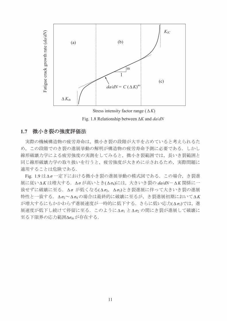
da/dN ΔKFig. 1.8
K (c) K da/dN Kmax
KIC
K (a) K da/dNK K Kth

10
K (b) K da/dN (1.15)
mKCdNda (1.15)
Paris C, m (8)
0
r
π ∆Kth
Fig. 1.7 Stress singularity and stress intensity factor at crack tip
0
11
1.7
Fig. 1.9 σ
K σ ( σ4) da/dN Kσ ( σ2 σ3)
σ2 σ4 K( σ1)
σ1 σ2
∆σth
Stress intensity factor range log(ΔK)
Fatig
ue c
rack
gro
wth
rate
log
(da/
dN) a
ΔK th
K fc
da /dN =C(ΔK )m
1m
(a ) (b )
(c )
Fig. 1.8 Relationship between ΔK and da/dN
KIC
Kth
(a) (b)
(c) da/dN = C ( K)m
Stress intensity factor range ( K)
Fatig
ue c
rack
gro
wth
rate
(da/
dN)

12
Fig. 1.9 Fatigue crack growth rate for various levels in stress amplitude Fig. 1.10 ∆σth a
K= Kth
∆σth ∆σw0
Fig. 1.10 An example of fatigue strength of SS400 with small crack
0.01 0.05 0.1 0.5 1 5 50
100
500
1000
Crack length a (mm)
Stre
ss
∆σth
(M
Pa)
Linear fracture mechanicsFatigue limit of smooth specimen
Kth : Constant
∆σw0
Stress intensity factor range K
Fatig
ue c
rack
gro
wth
rate
da
/dN
σ1< σ2< σ3< σ4
σ4
σ3 σ2
σ1
Final fracture
Big crack
Kth

13
El Haddad (9~12) El Haddada 0 a ( aa 0)
a 0
1.17 1.14 2
0
0
1
w
thKa
0aaKth (1.17)
1.17 a El Haddad a 0
aEl Haddad a 0
Fig. 1.11
0.01 0.05 0.1 0.5 1 550
100
500
1000
crack length a mm
Thre
shol
d St
ress
M
Pa
linear fracture mechanicsfatigue limit of smooth specimenEl Haddad equation
Fig. 1.11 Fatigue strength predicted using El Haddad equation for SS400 material
Linear fracture mechanicsFatigue limit of smooth specimen El Haddad equation
Crack length a (mm)
Stre
ss
w (
MPa
)
(1.16)

14
1.8
K
Point method Line method Area method 3
Fig. 1.12O Point method
rC
Line methodLC LC
Area method OAC
Point method ,
, Point method rC
rC
(1.5) 0 (13~17).
rKr2
(1.18)
rC (1.18) K Kth σ(r)σw0 r
2
21
wo
thC
Kr (1.19)

15
rC σw0
(1.5)(1.5) rC σw0 σy
(1.5)
cy r
Kr
K2
)2
3sin2
sin1(2
cos2
(1.20)
r=rC σy= σw0 σw(18~20)
r crack
rC
Δσw0 r
Kr th
2)(
σ
Fig. 1.13 Stress distributions near crack edge
Fig. 1.12 Point, line and area near circular hole in critical distance theory
O
LC rC

16
1.9
S20C Fig. 1.14
σw1
σw2 A B ρ0
σw1
ρ0
σw2(21)
ρ1 ρ0 σw2 σw1
ρ0 σw1
σ w1σ w
2,M
Pa
0
50
100
150
200
250
1 2 3 4 5
Stress concentration factor
σw1
σw2
ρ=1.0 mm
Fig. 1.14 S20C Fatigue strength of notched material
ρ0=0.5 mm
A
B

17
Table 1.1(2,22,23) ρ0
Table 1.1 Critical radius ρ0 for each materials. Material σB
MPa σS
MPa σw0
MPa ρ0
mm S10C Carbon steel 372 203 181 0.6 S20C Carbon steel 469 279 211 0.5 S25C Carbon steel 494 297 255 0.5 S35C Carbon steel 600 336 274 0.4 S50C Carbon steel 673 347 265 0.25
S50C Carbon steel refining 1010 858 500 0.1 S50C Carbon steel refining 1246 1132 617 0.1
SNCM26 Nickel-chromium-molybdenum steel 1389 1140 629 0.1 σB: Tensile strength σS: Yield stress σw0: Fatigue limit ρ0: Notch radius

18
2
2.1
100
SS400V
SS400
2.2
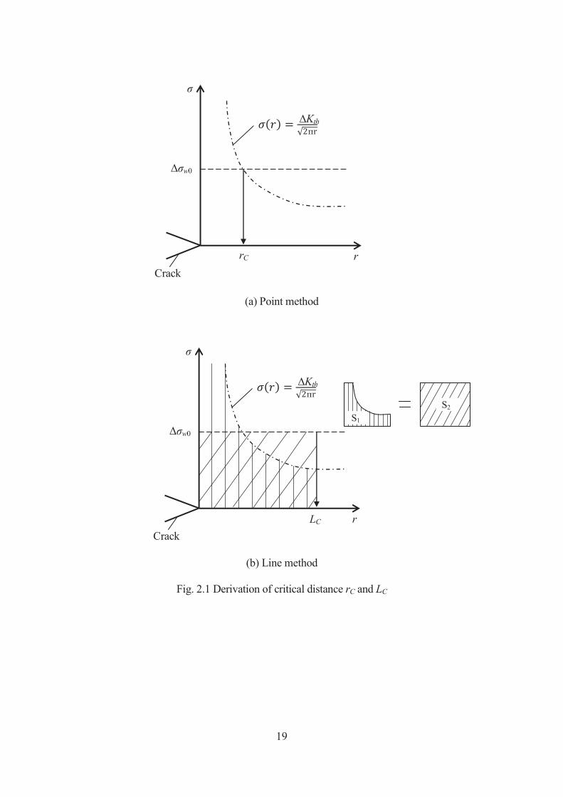
Fig. 2.1 ∆σw0
∆Kth rC Point methodLC Line method
. rC LC
.
rC=(∆Kth /Δσw0)2/2 π (Point method) (2.1) LC=2(∆Kth /Δσw0)2/π
(2.2) (Line method)
19
(a) Point method
(b) Line method
Fig. 2.1 Derivation of critical distance rC and LC
Crack r
σ
π ∆Kth
Δσw0
rC
Crack r
σ
π ∆Kth
Δσw0
LC
S1
S2
20
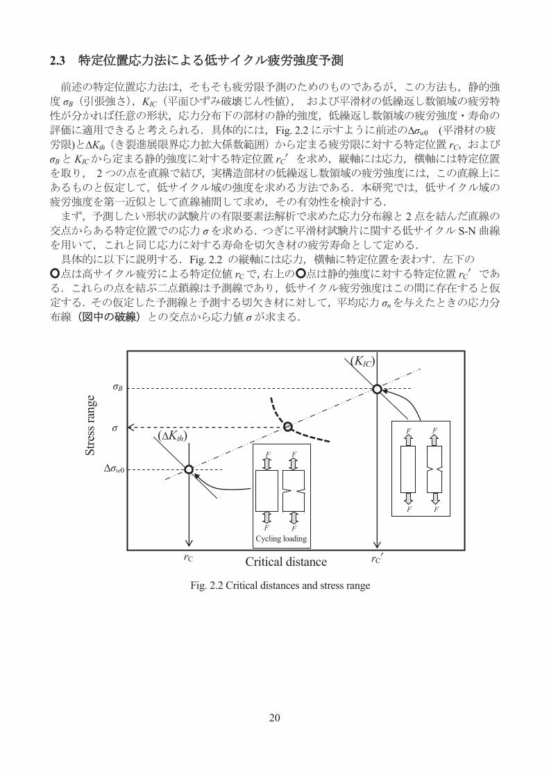
2.3
σB KIC
Fig. 2.2 ∆σw0 () ∆Kth rC
σB KIC rC
2
2
σ S-N
Fig. 2.2 rC rC
σn
σ
Fig. 2.2 Critical distances and stress range
rC
F
F
F
F
Critical distance
Stre
ss ra
nge
rC
σ
σB
∆σw0
(∆Kth)
(KIC)
Cycling loading
F
F
F
F
21
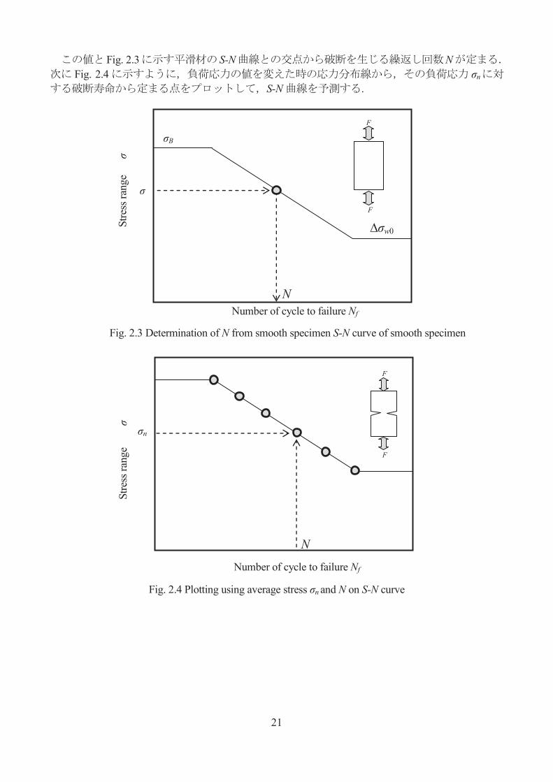
Fig. 2.3 S-N NFig. 2.4 σn
S-N .
Fig. 2.3 Determination of N from smooth specimen S-N curve of smooth specimen
Fig. 2.4 Plotting using average stress σn and N on S-N curve
σB
∆σw0
σ
N Number of cycle to failure Nf
Stre
ss ra
nge
σ
σn
N
Stre
ss ra
nge
σ
Number of cycle to failure Nf
F
F
F
F

22
2.3.1
σ N V10t
EHF-EA10 4830Fig. 2.5
R 0 20Hz
N 5 106
2 kN
Table 2.1 SS400(20) Fig. 2.6 .

23
Fig. 2.5 General view of fatigue testing apparatus
∆σw0 (MPa)
∆Kth (MPa m1/2)
σB (MPa)
KIC
(MPa m1/2) 305 6.7 448 39.5
Hydraulic unit
Testing machine
Servo controller
Load cell
Specimen
Hydraulic actuator
Table 2.1 Mechanical properties of SS400 steel

24
(a) Smooth specimen
(b) V-notch specimen
(c) Circular hole specimen Fig. 2.6 Dimensions of specimens
rC rC (2.1),(2.2)
rC = (∆KIC /ΔσB)2/2 π = 1.240 mm ( )
rC (∆Kth /Δσw0)2/2 π= 0.077 mm ( )
4 mm or 10 mm
60 or 120
8- 10
8- 10
8- 10
15

25
2.3.2
NX NASTRAN 1/4 V
Fig. 2.7 200 MPa 450 MPaTable 2.2 5 mm
(a) V-notch specimen (1/4 region)
(b) Circular hole specimen (1/4 region)
Fig. 2.7 Finite element meshes
Element type 2-Dimensional 6 node triangular element (PLANE183) Element model Plane stress condition
Material property Linear elastic body Young's modulus 210 GPa Poisson's ratio 0.3
Table 2.2 Calculation condition of FEM analysis

26
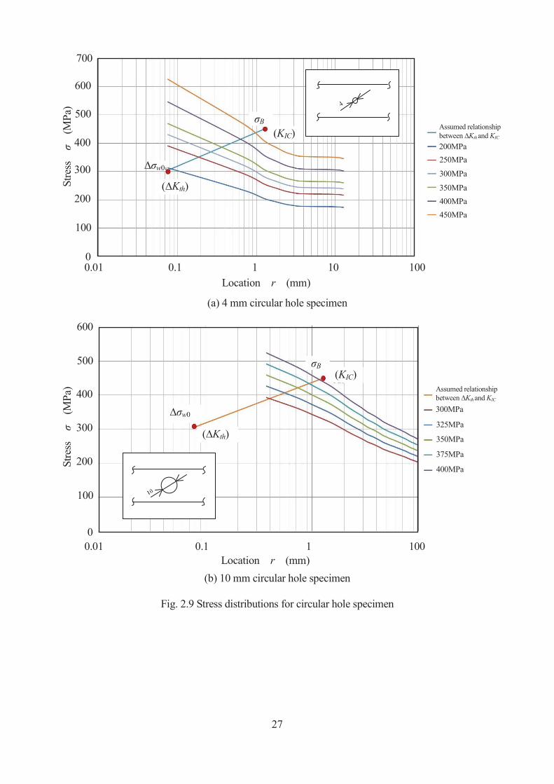
V 60° 120° Fig. 2.8
4 mm10 mm Fig. 2.9
(a) 60° V-notch specimen
(b) 120° V-notch specimen
Fig. 2.8 Stress distributions for V-notch specimen
Location r (mm)
Stre
ss σ
(M
Pa)
Location r (mm)
Stre
ss σ
(M
Pa)
(KIC)
(KIC)
σB
σB
(∆Kth)
(∆Kth)
Assumed relationship between ∆Kth and KIC
200MPa 250MPa 300MPa 350MPa 400MPa
450MPa
60
120
Assumed relationship between ∆Kth and KIC
250MPa 300MPa 320MPa 335MPa 350MPa 370MPa
0.01 0.1 1 10 100
0.01 0.1 1 10 100
1000
800
600
400
200
0
500
400
300
200
100
0
∆σw0
∆σw0
27
(a) 4 mm circular hole specimen
(b) 10 mm circular hole specimen
Fig. 2.9 Stress distributions for circular hole specimen
Location r (mm)
Stre
ss σ
(M
Pa)
Location r (mm)
Stre
ss σ
(M
Pa)
(KIC)
(KIC)
σB
σB
(∆Kth)
(∆Kth)
∆σw0
Assumed relationship between ∆Kth and KIC
200MPa 250MPa
300MPa
350MPa 400MPa 450MPa
Assumed relationship between ∆Kth and KIC
300MPa
325MPa
350MPa
375MPa
400MPa
600
500
400
300
200
100
0 0.01 0.1 1 100
600
500
400
300
200
100
0
700
0.01 0.1 1 10 100
∆σw0
28
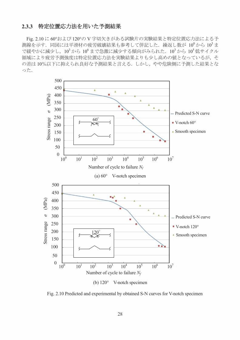
2.3.3
Fig. 2.10 60° 120° V 100 103
103 106 103 105
10
(a) 60° V-notch specimen
(b) 120° V-notch specimen
Fig. 2.10 Predicted and experimental by obtained S-N curves for V-notch specimen
Number of cycle to failure Nf
Number of cycle to failure Nf
100 101 102 103 104 105 106 107
100 101 102 103 104 105 106 107
Predicted S-N curve
V-notch 60°
Smooth specimen
Predicted S-N curve
V-notch 120°
Smooth specimen
Stre
ss ra
nge
σ
(MPa
)
500 450 400 350 300 250 200 150 100 50 0
120
500 450 400 350 300 250 200 150 100
50 0
Stre
ss ra
nge
σ
(MPa
)
60
29
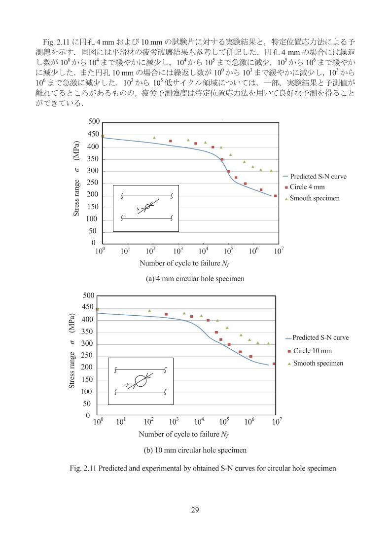
Fig. 2.11 4 mm 10 mm4 mm
100 104 104 105 105 106
10 mm 100 103 103
106 103 105
(a) 4 mm circular hole specimen
(b) 10 mm circular hole specimen
Fig. 2.11 Predicted and experimental by obtained S-N curves for circular hole specimen
Number of cycle to failure Nf 100 101 102 103 104 105 106 107
Predicted S-N curve Circle 4 mm Smooth specimen
Predicted S-N curve
Circle 10 mm
Smooth specimen
Stre
ss ra
nge
σ
(MPa
) St
ress
rang
e σ
(M
Pa)
500 450 400 350 300 250 200 150 100 50 0
500 450 400 350 300 250 200 150 100 50 0
100 101 102 103 104 105 106 107
Number of cycle to failure Nf

30
2.4
2 S-N
(24~27) (27~28)
(29~31)
DSS(Daily Start Stop)Fig. 2.12
(30,31)
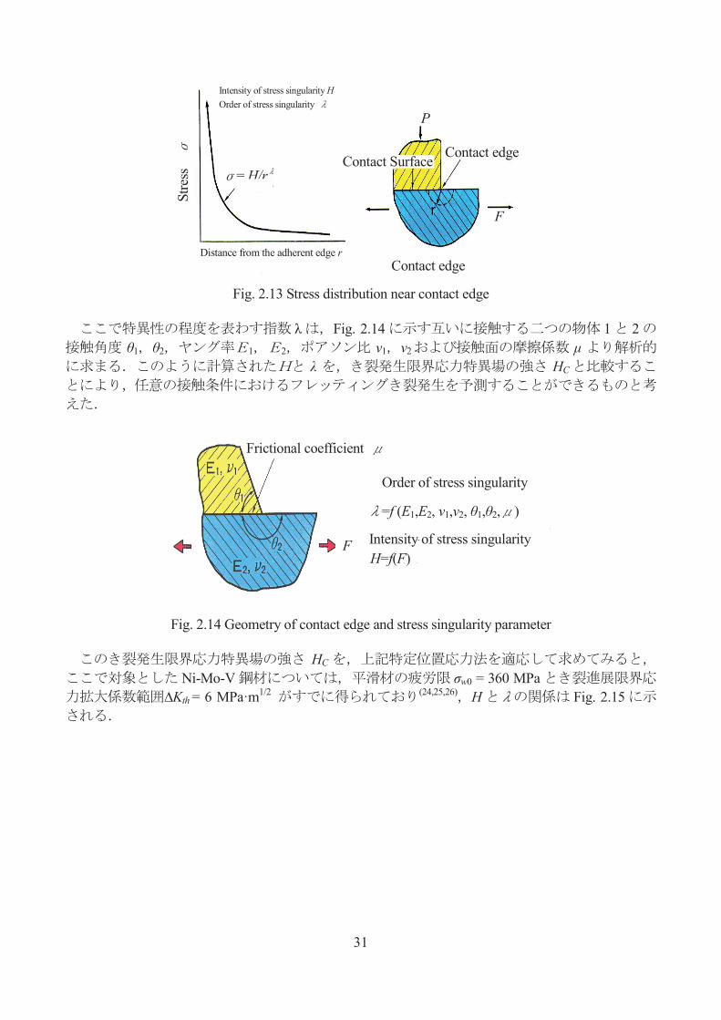
Fig. 2.13H r
rH / (2.3)
High cycle fatigue
Low cyclefatigue
Time t
Stre
ss σ
Fig. 2.12 Assembled gas-turbine compressor rotors and blade dovetail joint
31
Fig. 2.13 Stress distribution near contact edge
λ Fig. 2.14 1 2
θ1 θ2 1 2 ν1 ν2 μλ HC
Fig. 2.14 Geometry of contact edge and stress singularity parameter
HC
Ni-Mo-V σw0 = 360 MPa∆Kth = 6 MPa·m1/2 (24,25,26) H Fig. 2.15
H=f(F)
Intensity of stress singularity H Order of stress singularity
= H/r St
ress
Distance from the adherent edge r Contact edge
Contact edge Contact Surface
P
F
Frictional coefficient
F Intensity of stress singularity
Order of stress singularity
=f (E1,E2, ν1,ν2, θ1,θ2, )

32
0 0.1 0.2 0.3 0.4 0.50
200
400
Fig. 2.15 Fretting fatigue crack initiation criteria using stress singularity
parameters derived from critical distance theory
(26) Fig. 2.16 90°65° Δσθ Fig. 2.17
(2.1) rC = 0.11mm
Fig. 2.16 Contact model for initiation of fretting fatigue crack
Line method
Point method
Order of stress singularity
Inte
nsity
of s
tress
sing
ular
ity H
Contact pressure P
Contact edge
Axial load σa
Pad
Contact surface
Specimen
33
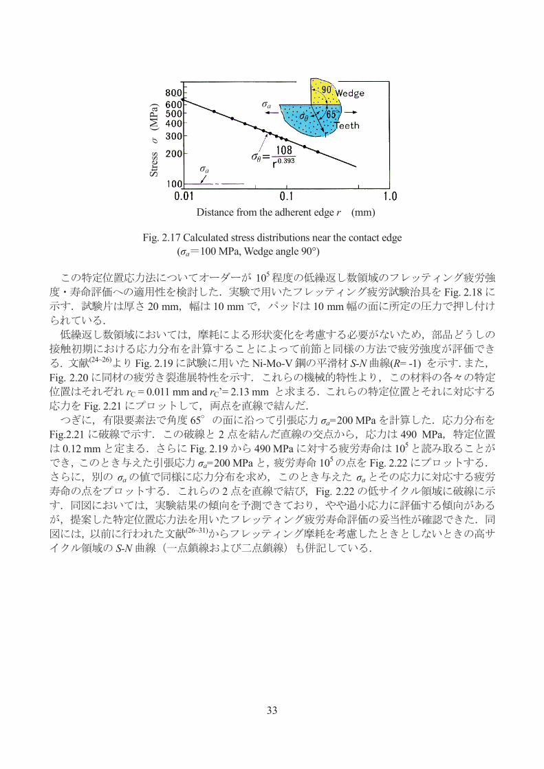
Fig. 2.17 Calculated stress distributions near the contact edge (σa 100 MPa, Wedge angle 90°)
105
Fig. 2.1820 mm 10 mm 10 mm
. (24~26) Fig. 2.19 Ni-Mo-V S-N (R= -1) Fig. 2.20
rC = 0.011 mm and rC’= 2.13 mm Fig. 2.21
65 σa=200 MPaFig.2.21 2 490 MPa
0.12 mm Fig. 2.19 490 MPa 105
σa=200 MPa 105 Fig. 2.22σa σa
2 Fig. 2.22
(26~31)
S-N
σa
σa
Distance from the adherent edge r (mm)
Stre
ss
(M
Pa)

34
Fig. 2.18 Fretting fatigue test apparatus
103 104 105 106 107 108100
1000
Fig. 2.19 S-N Curve of Ni-Mo-V steel smooth specimen
Estimated cycle to failure
Number of cycle to failure Nf
Stre
ss ra
nge
σa
(M
Pa)
σB = 705 MPa
∆σw0 = 360 MPa
Specimen
Pad Strain gage B
Screw
Press plate Strain gage A
20
10
10
40

35
1 10 10010−12
10−10
10−8
10−6
Fig. 2.20 Crack propagation rate of Ni-Mo-V steel
0.01 0.1 1 10100
1000
Fig. 2.21 Derivation of specific distance in low cycle fatigue region and estimation of low cycle fretting fatigue life fatigue
Crac
k pr
opag
atio
n ra
te d
a/dN
, m/c
ycle
Stress intensity factor range ∆K, MPa·m1/2
da/dN=C(∆K)m
R=0
Stre
ss
σ
(MPa
)
Distance r (mm)
σa = 200 MPa
σB
(KIC)
(∆Kth)
∆σw0
705
360
1000
100
Stress distribution obtained by FEM
0.01 0.1 1 10

36
103 105 106 107 108104
100
500
1000
Number of cycles to failure Nf
Str
ess
am
plit
ude
σ
a(M
pa)
Plane specimen
Fretting (Low cycle)
Fretting(Ultra high cycle)
Experimental
Smooth specimen
Fig. 2.22 Estimated and experimental fretting fatigue S-N Curves
a: Prediction from(30,31) b: Prediction from(30,31)
2.5
SS400 V
(1)
(2) 103 105 V
10 %
(3) 10 %
V
(4)
V
Number of cycles to failure Nf
Stre
ss a
mpl
itude
σ a
(MPa
)
(a)
(b)

37
3
3.1
2 Point method
FEMSS400 SKS93
S-N SS400SKS93
3.2
KI
)(FaK F(ξ) ξ
W ξ = a / W (5 7)
2c o s
2s i n1199.0923.0
2tan2)(
4
F
Δσw0 El Haddad
a0
a ( a + a0 )(10)
)(/ 0Δ aaKthE a 0 Δσw0 a0
2
00
1w
thKa
a a0
a a0
ΔK ΔKth
(3.1)
(3.2)
(3.4)
(3.3)
ΔΔ
38
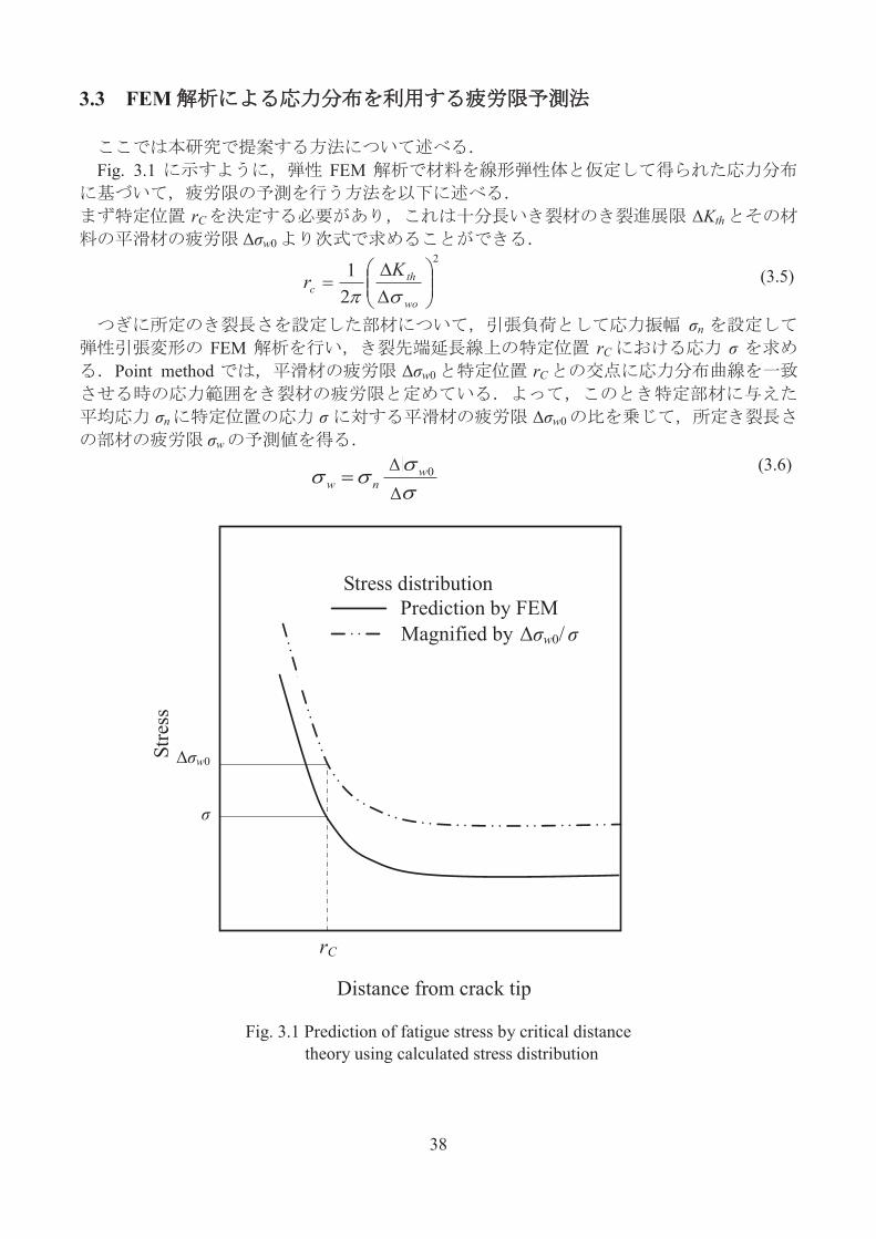
3.3 FEM
Fig. 3.1 FEM
rC ΔKth
Δσw0
2
21
wo
thc
Kr
σn
FEM rC σPoint method Δσw0 rC
σn σ Δσw0
σw
0w
nw
rc
Distance from crack
Stress distribution Prediction by FEM Magnified by σw0 / σ
σw0
σ
Fig. 3.1 Prediction of fatigue stress by critical distance theory using calculated stress distribution
(3.5)
(3.6)
rC
Distance from crack tip
Stress distribution Prediction by FEM Magnified by
ΔΔ
Δσw0/ σ
Δσw0
σ
Stre
ss
39
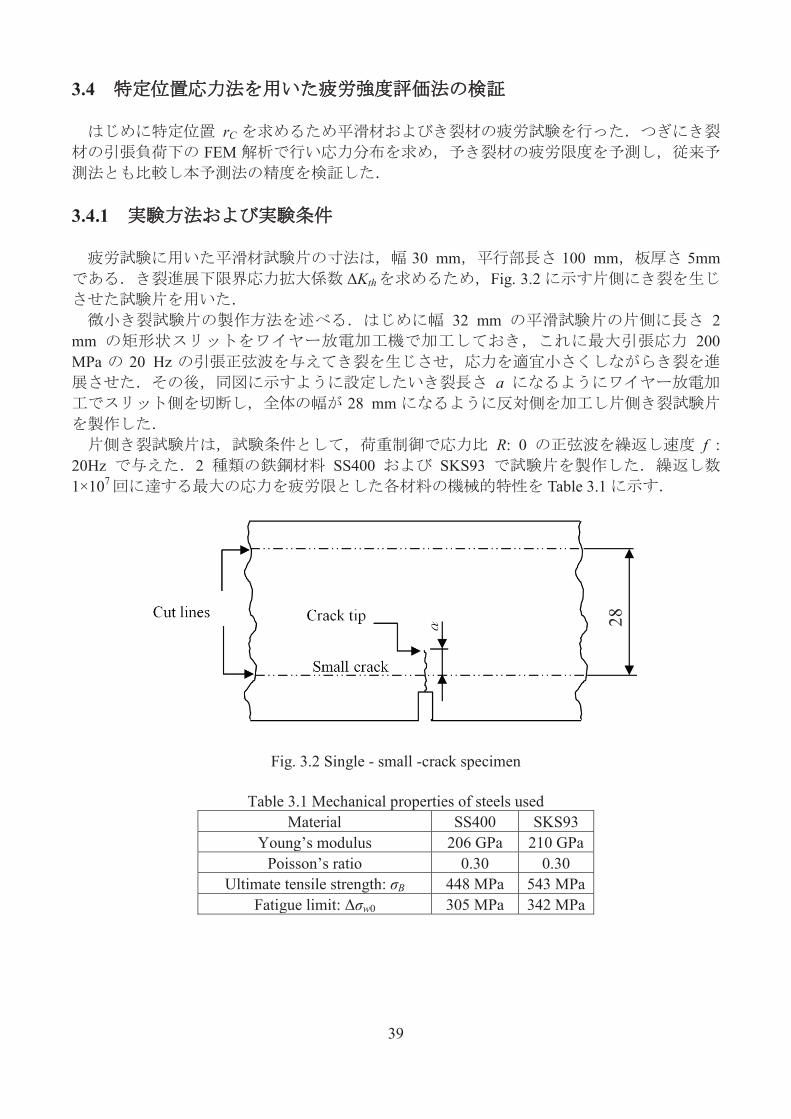
3.4
rC
FEM
3.4.1
30 mm 100 mm 5mmΔKth Fig. 3.2
32 mm 2
mm 200 MPa 20 Hz
a28 mm
R: 0 f :
20Hz 2 SS400 SKS931×107 Table 3.1
Fig. 3.2 Single - small -crack specimen
Table 3.1 Mechanical properties of steels used Material SS400 SKS93
Young’s modulus 206 GPa 210 GPa Poisson’s ratio 0.30 0.30
Ultimate tensile strength: σB 448 MPa 543 MPa Fatigue limit: Δσw0 305 MPa 342 MPa
28

40
3.4.2
SS400 SKS93 Fig. 3.3 ○0.1 mm ( KV - 5C) ΔK
□ 0.1 mm 1 mm ( KV - 25B)
Paris mKcdNda / (3.7)
SS400 8MPa·m1/2 6.7 MPa·m1/2
SS400ΔKth 6.7 MPa·m1/2 SKS93 8.1 MPa·m1/2
Table 3.2Δσw0 ΔKth (4) (5)
rC El Haddad a0 Table 3.2
Table 3.2 Critical distance and potential crack length Material SS400 SKS93
Critical distance rC 0.077 mm 0.089 mm Potential crack length a0 0.154 mm 0.179 mm

41
10-4
10-5
10-6
10-7
σ= Const
K- Decreasing procedure
100 101 102
10-4
10-5
10-6
10-7
σ= Const
K- Decreasing procedure
100 101 102
1 2 3 4 5 678910 20 30405060708090100
10−10
10−8
10−6
10−4
100 101 102
10-4
10-5
10-6
10-7
10-8
10-9
10-10
10-11
interval 0.1mm K-decreasing procedure
interval 1mm σ= const
interval 0.1mm σ= const
(a) Material: SS400
(b) Material: SKS93
Fig. 3.3 Fatigue crack growth rate
Stress intensity factor range ΔK (MPa m1/2)
Fatig
ue c
rack
gro
wth
rate
d
a/dN
(mm
/cyc
le)
Stress intensity factor range ΔK (MPa m1/2)
Fatig
ue c
rack
gro
wth
rate
d
a/dN
(m
m/c
ycle
)
Grid interval 0.1 mm, ΔK-decreasing procedure
Grid interval 1 mm, Δσ = Const
Δσ = Const
ΔK-decreasing procedure
Grid interval 0.1 mm, Δσ = Const
10-4
10-5
10-6
10-7
100 101 102
42
3.4.3 FEM
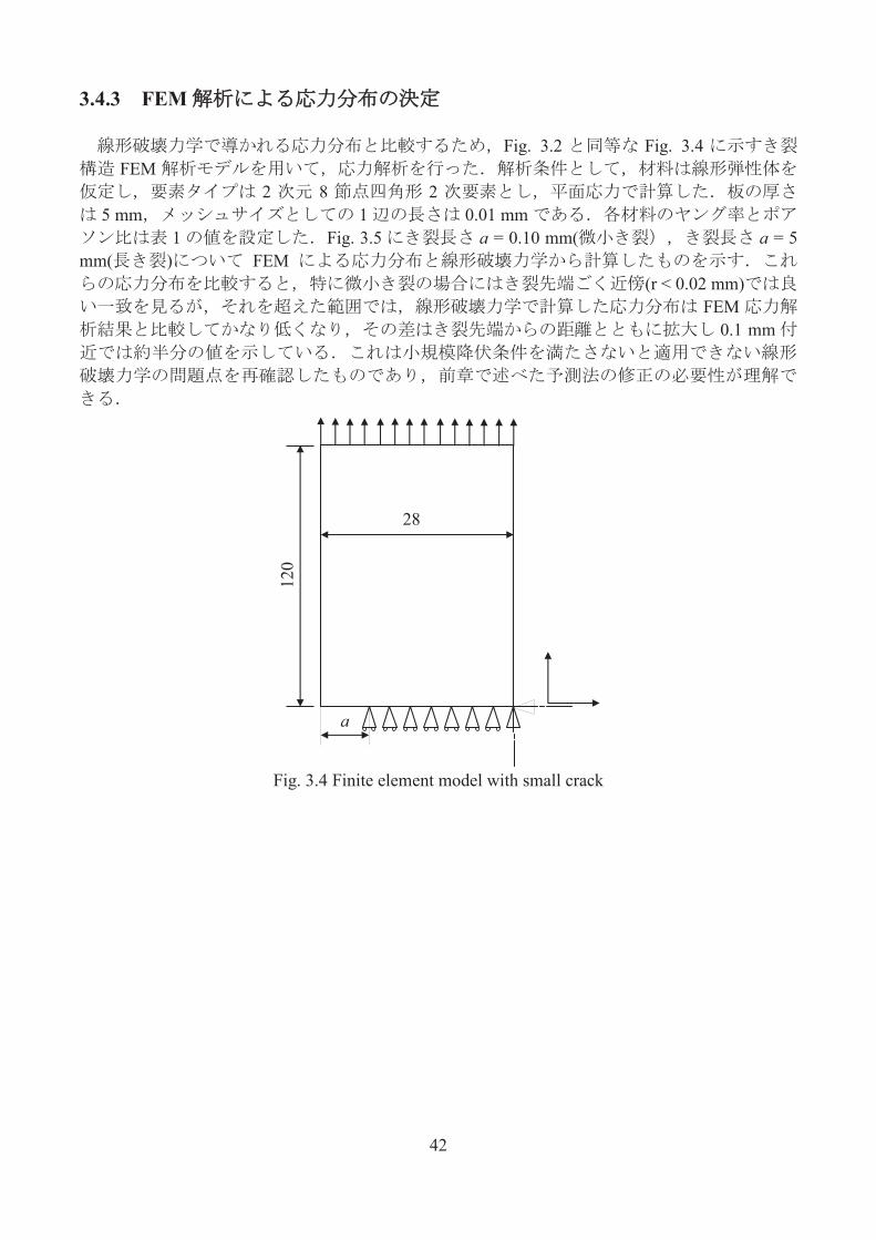
Fig. 3.2 Fig. 3.4FEM
2 8 25 mm 1 0.01 mm
1 Fig. 3.5 a = 0.10 mm( a = 5 mm( ) FEM
(r < 0.02 mm)FEM
0.1 mm
Fig. 3.4 Finite element model with small crack
a
28
120

43
0 0.10
100
200
0 0.02 0.04 0.06 0.08 0.1
200
Distance r (mm)
Stre
ss σ
(MPa
)100
Linear fracture mechanicsFEM
0
(a) a: 0.10 mm , σ: 100 MPa
0 0.10
500
1000
1500Linear fracture mechanicsFEM
500
1000
1500
0 0.02 0.04 0.06 0.08 0.1
Stre
ss σ
(MPa
)
Distance r (mm)
0
(b) a: 5 mm , σ:100 MPa
Fig. 3.5 Stress distribution near crack tip

44
5 10 15 [ 10+6]300
310
320
330
3.4.4
0.10 0.50 1.00 5.00 10.00 mmσn 100 MPa
σ (3.6) σw 3.4.1
1×10⁷
Fig. 3.23 4 SKS93 ,
0.112 mm S-N Fig. 3.6
Fig. 3.6 Experimental results of fatigue limit of cracked specimens (SKS93 Steel, Cracked length 0.112 mm)
σw 310 MPa
El Haddad Fig. 3.7
Table 3.3 Δσw0 / σσw Table 3.2 a0 (3) El Haddad
σE El Haddad
Fig. 3.7 Table 3.3
10 mm Table 3.328 mm 1/3
Fig. 3.7 0.1mm(SS400:305MPa ,SKS93:342
MPa) 0.1 mm (SS400:299MPa,SKS93:329MPa)1 mm
El Haddad 0.1 mm
Stre
ss ra
nge
Δσ n
(M
Pa)
300
330
320
310
106 107 Number of cycle to failure Nf

45
0.1 mm 1 mm
(a) Material : SS400
(b) Material : SKS93
Fig. 3.7 Comparison of prediction methods for crack specimens of steel plate
Fatig
ue li
mit
σ w
(MPa
) Fa
tigue
lim
itσ w
(M
Pa)
Crack length a (mm)
Crack length a (mm)
Fatigue test result Fatigue limit of smooth specimen Critical distance theory El Haddad Linear fracture mechanics
Fatigue test result Fatigue limit of smooth specimen Critical distance theory El Haddad Linear fracture mechanics

46
3.5
SS400 SKS93
(1) 0.1 mm
(2) SS400 SKS93 0.1 1 mm
(3)
El Haddad 0.1 mm
(4)
Table 3.3 Fatigue limit result for each crack length of SS400 and SKS93 steel
Material SS400 SKS93 Crack length a (mm) Δσw0 / σ σw (MPa) σE (MPa) Δσw0 / σ σw (MPa) σE (MPa)
0.10 2.985 299 239 3.290 329 273 0.50 1.586 159 148 1.868 187 175 1.00 1.111 111 111 1.325 133 133 5.00 0.446 45 53 0.500 50 63 10.00 0.204 20 38 0.243 24 45
47
4
SS400 V
(1)
(2) 103 105 V
10 %
(3)
10 % V
(4)
V
S-NSS400 SKS93 El Haddad
(1) 0.1 mm
(2) SS400 SKS93 0.1 1 mm
(3)
El Haddad 0.1 mm
(4)

48

49
1) (2004) 167-170
2) (1995) 19-28
3) (1967)
4) (1984)
5) (2006) 23-26
6) (1995) 149-155
7) Vol. 1, (1983), 32
8) (2006) 88-94, 132-135
9) El Haddad, M.H.,Smith,K.N. and Topper, T. H.: Fatigue Crack Propagation of Short Crack,
Trans. ASME, J. Eng. Mater. Tech., 101, (1979), 42.
10) El Haddad,M.H.,Topper,T.H.and Smith,K.N.:Prediction of non propagating
cracks.Engng.Fract.Mech.,11, (1979), 573.
11) El Haddad,M.H.,Dowling,N.E.,Topper,T.H.and Smith,K.N.:J-Integral application to short fatigue
cracks at notches. Int.J.Fract.,16, (1980) ,15.
12) Shin,C.S. and Smith,K.N.:Fatigue crack growth from sharp notches.Int.J.Fatigue,7, (1985) ,87.
13) David Taylor Geometrical effects in fatigue; a unifying theoretical model International Journal
of Fatigue 21 1999),413.
14) D. Taylor, The Theory of Critical Distances: A New Perspective in Fracture Mechanics. Elsevier,
Oxford, UK (2007).
15)
2005)
16)
, (A ) 54 499 (1988), 597.
17) ,
(A ) 67 661 (2001) ,1486.
18) Nakamura, F., Abe, T., Hattori, T and Yamashita, M.: Fatigue Strength Evaluation Methods
Using Stress Distributions, Key Engineering Materials, 417-418 (2010), 409.
19) Hattori, T., Amiruddin, M., Ishida, T. and Yamashita, M.: Fretting Fatigue Life Estimations
Based on the Critical Distance Stress Theory, Procedia Engineering, 10 (2011), 3134

50
20) Amiruddin, M., Jie, N., Hattori, T. and Yamashita, M.: Fatigue Strength and Life Estimation
Methods Using Critical Distance Stress Theory, Advanced Materials Research,Vols. 694-697
(2013),853.
21) 42, (1976),996.
22) 26 1977 296.
23) 34 1968 371.
24) Hattori T. Sakata H. and Watanabe T. A stress singularity parameter approach for evaluating adhesive and fretting strength ASME Book No. G00485 MD-vol.6 (1988)43.
25) Hattori T. and Nakamura N. Fretting fatigue evaluation using stress singularity parameters at contact edges Fretting Fatigue ESIS Publication 18 (1994), 453.
26) Hattori T. Nakamura M. and Watanabe T. Simulation of fretting fatigue life by using stress singularity parameters and fracture mechanics Tribology International ( 2003) 36 87.
27) Hattori T. et al. Fretting fatigue analysis using fracture mechanics JSME Int. J Ser. l (1988) 31 100.
28) Suresh S. Fatigue of Materials 2nd Edition Cambridge University Press (1998) 469 29) Goryacheva I. G. Rajeev P. T. and Farris T. N. Wear in partial slip contact ASME
J. of Tribology (2001) 123 4,848. 30) Hattori T. Yamashita M. and Nishimura N. Fretting fatigue strength and life estimation
in high cycle region considering the fretting wear process JSME International Journal ( 2005) 48,4,246.
31) Hattori T. Nakamura Nishimura N. and Yamashita M. Fretting fatigue strength estimation considering the fretting wear process Tribology International (2006),39 1100.

51
MUHAMMAD AMIRUDDIN BIN AB WAHAB