Comparison of Three Control Methods for an Autonomous Vehicle

Anup Deshpande, Kovid Mathur and Ernest Hall

Center for Robotics Research

University of Cincinnati

Cincinnati, OH 45221-0072 USA

Phone: 513-556-2730

Fax: 513-556-3390

www.robotics.uc.edu

ABSTRACT

The desirability and challenge of developing a completely autonomous vehicle and the rising need for more efficient use

of energy by automobiles motivate the search for an optimum solution to computer control of energy efficient vehicles.

The purpose of this paper is to compare three control methods - mechanical, hydraulic and electric that have been used

to convert an experimental all terrain vehicle to drive by wire which would eventually act as a test bed for conducting

research on various technologies for autonomous operation. Computer control of basic operations in a vehicle namely

steering, braking and speed control have been implemented and will be described in this paper. The output from a 3 axis

motion controller is used for this purpose. The motion controller is interfaced with a software program and WSDK

(Windows Servo Design Kit) serves as an intermediate tuning layer for tuning and parameter settings in autonomous

operation. The software program is developed in C++. The voltage signal sent to the motion controller can be varied

through the control program for desired results in controlling the steering motor, activating the hydraulic brakes and

varying the vehicle’s speed.

The vehicle has been tested for its basic functionality which includes testing of street legal operations and also a 1000

mile test while running in a hybrid mode. The vehicle has also been tested for control when it is interfaced with devices

such as a keyboard, joystick and sensors under full autonomous operation. The vehicle is currently being tested in

various safety studies and is being used as a test bed for experiments in control courses and research studies. The

significance of this research is in providing a greater understanding of conventional driving controls and the possibility

of improving automobile safety skills.

Keywords: Intelligent autonomous vehicle, electrical control, hydraulic control, mechanical control, human interface.

1. INTRODUCTION

An experimental all terrain vehicle was made street legal and modified to drive by wire for the 2007 DARPA Urban

Challenge which would also serve as a test bed for further studies in energy efficiency, safety and educational

purposes. In order for the experimental vehicle to be street legal it was required to have head/indicator lights, a safety

glass windshield followed by an inspection by the State Patrol. The successful inspection then permitted the registration,

license and insurance of the vehicle. The conversion of the vehicle to drive by wire mode required several design

changes in the steering, speed control and brake system. Since this 2100 pound vehicle can reach speeds of 45 mph with

its two 7.5HP electric motors, safety was of primary concern. For this reason, an emergency stop and a back up signal

were added. A wireless remote emergency stop was also made available and a chase vehicle was always used for street

testing.

The reasons for performing this study and conducting further research in the field of autonomous vehicle control are as

follows.

1) A fully electric vehicle is a step towards energy efficiency.

2) Implementation of computer control of basic automobile operations like speed, steering, and braking control permits

the exploration of new ways for computer control of automotive operations.

3) The computer control and further research work to address existing unresolved problems can eliminate the need or

augment the actual physical control by the user, which can be helpful to people with physical limitations.

4) Implementation of the modern tools like artificial neural networks and computer vision can also be used to detect

faults and assist users with obstacle avoidance as collisions cause most injuries to humans.

5) Electric and hybrid vehicles are now available for transportation and robotics is the modern tool for automation. The

combination of these technologies can results in new solutions to a variety of applications.

The study of autonomous operation of automobiles can improve the reliability both in terms of the safety of its operation

as well as minimal consumption of energy. The problem of autonomous vehicle control may be modeled as a dynamic

programming problem.1 However, the gap between theory and practice is still rather large. It has been made smaller by

experimental studies conducted at the Intelligent Ground Vehicle Contest (www.igvc.org ) that has been conducted since

1993 which has resulted in many technical advances on small sized unmanned ground vehicles. Larger experimental

vehicles have been motivated by the DARPA Grand Challenges in 2004 and 2005 and the Urban Challenge in 2007.

Thrun 2

describes the winning vehicle for the 2005 Grand Challenge. Urmson, el al. 3 describe the 2007 winning team

and vehicle. Most of the vehicles in the Urban Challenge were “production vehicles.” However, various “self

constructed” vehicles were also eligible with additional qualifications.

The purpose of this paper is to compare and contrast three methods for vehicle control – mechanical, hydraulic and

electrical. For definiteness, an example of an experimental “self constructed” vehicle is used which was modified for

various needs at the University of Cincinnati.

The steering control will be described in Section 2, brake control in Section 3 and vehicle speed control in Section 4.

Finally, a comparison of the methods and experimental results are given in Sections 5 and 6.

2. STEERING CONTROL

A servo control system is used in the electric ATV (All terrain vehicles) to steer the wheels. It comprises of a motor, an

encoder and an amplifier. A gearbox with gear ratio 10:1 is used to be able to turn the wheels from full left to full right in

100 motor turns which would give us an acceptable response time for real time operations.

Figure 1. Elements of servo system

1.1Servo control system elements

Motor: A motor converts current into torque which produces motion. The desired motion in our case is the steering of

the wheels with its extremes being a full left or full right turn. In a motion controller, each axis of motion requires a

motor sized properly to move the desired load at the desired speed and acceleration. The motor may be a step or servo

motor and can be brush type or brushless, rotary or linear. For our application a rotary, brush type DC servomotor is

used.

Amplifier: An amplifier is a device that modifies (usually increases) the amplitude of an incoming signal. In our circuit,

the power amplifiers convert input voltage signals from the controller into current required to drive the motor. For best

performance the amplifier should be configured for a current mode of operation with PID compensation.

Encoder: An encoder translates motion into electrical pulses which are fed back into the controller. Encoders typically

provide two channels in quadrature, channel A and channel B. This type of encoder is called a quadrature encoder. The

channels A and B are 90 degrees out of phase and due to this relationship, the resolution of the encoder is increased to

4N quadrature counts/rev. (N is the number of pulses generated by the encoder per revolution).

1.2 Digital-controlled servo system

A servo system is a closed loop motor control system that combines various components to automatically and accurately

control a machine’s operation4. It is generally composed of a servo drive, a motor, and a feedback device. The controller

receives an outside command signal and a feedback signal from the motor which get summed up and a resultant signal is

sent which controls the torque, velocity and position of the motor shaft. The feedback continuously reports the real time

status, which is constantly compared with the command value. Differences between the command position and feedback

signals are automatically adjusted by the closed-loop servo system. This closed-loop provides the servo system with

accurate, high performance control of a machine.

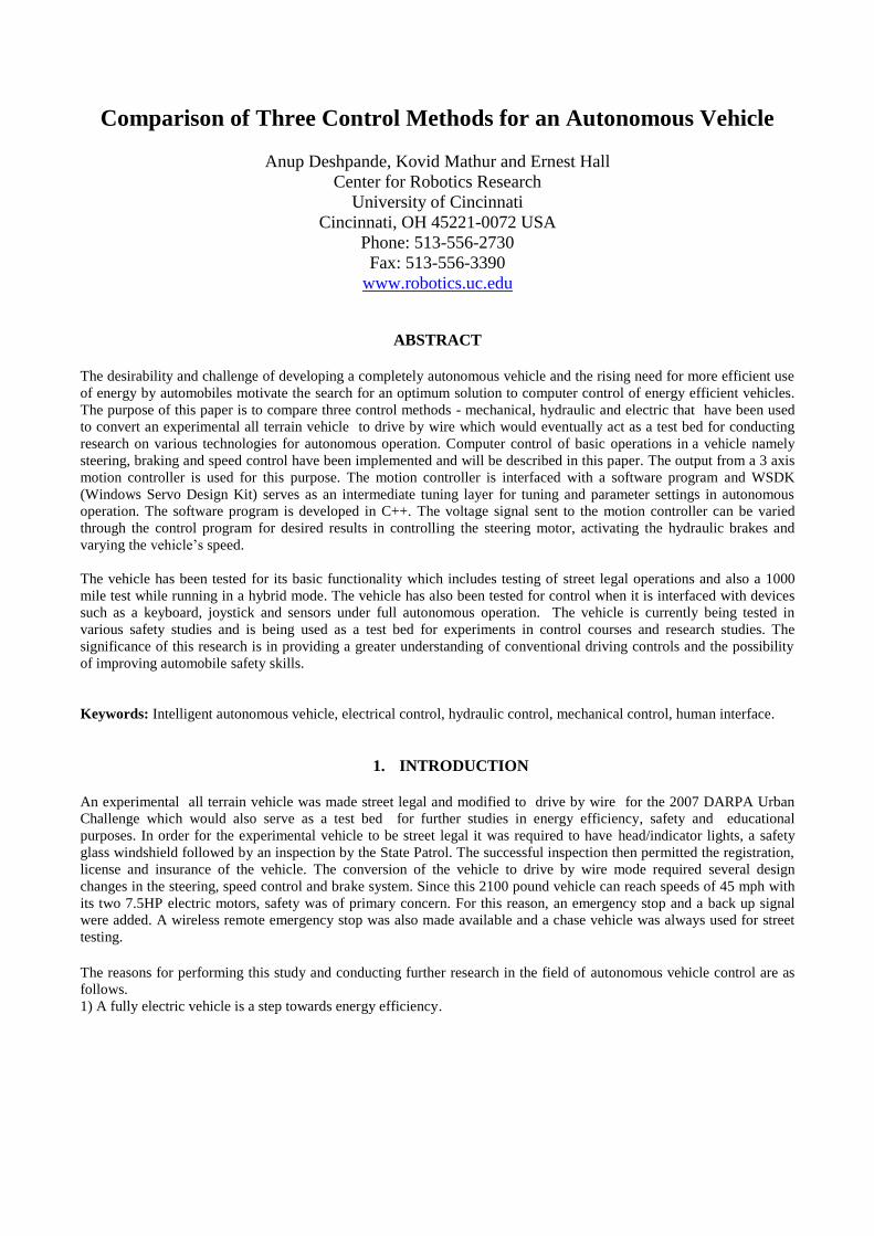
Figure 2. Functional elements of a computer controlled servo system

(a) block diagram (b) the controller4

A typical computer-controlled servo system is shown in Figure 2. It has three main elements, a digital controller, an

amplifier, and a motor combined with an encoder. The controller is composed of a digital filter, a zero-order-hold (ZOH)

and a Digital to Analog Converter (DAC). The purpose of the controller is to compensate for the system to make an

unstable system become stable. This is usually achieved by adjusting the parameters of the filter. The controller accepts

both encoder feedback and commands from the computer and finds the error between them. The error signal then passes

through the digital filter, ZOH and DAC to generate control signals to control the amplifier (AMP). The amplifier

amplifies the control signals from the controller to drive the motor. The encoder is usually mounted on the motor shaft.

When the shaft moves, it generates electrical impulses, which are processed into digital position information. This

position information is then fed back directly into the controller. The mathematical model of the above components

could be varied among different products.

1.3 Computer control of the steering mechanism

Figure 3 shows the computer control of the steering mechanism. It involves a servo system and a motion controller. The

motion controller serves as an interface between the computer program (to provide command signals) and the servo

system.

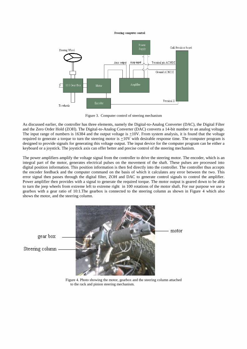
Figure 3. Computer control of steering mechanism

As discussed earlier, the controller has three elements, namely the Digital-to-Analog Converter (DAC), the Digital Filter

and the Zero Order Hold (ZOH). The Digital-to-Analog Converter (DAC) converts a 14-bit number to an analog voltage.

The input range of numbers is 16384 and the output voltage is +10V. From system analysis, it is found that the voltage

required to generate a torque to turn the steering motor is +10V with desirable response time. The computer program is

designed to provide signals for generating this voltage output. The input device for the computer program can be either a

keyboard or a joystick. The joystick axis can offer better and precise control of the steering mechanism.

The power amplifiers amplify the voltage signal from the controller to drive the steering motor. The encoder, which is an

integral part of the motor, generates electrical pulses on the movement of the shaft. These pulses are processed into

digital position information. This position information is then fed directly into the controller. The controller thus accepts

the encoder feedback and the computer command on the basis of which it calculates any error between the two. This

error signal then passes through the digital filter, ZOH and DAC to generate control signals to control the amplifier.

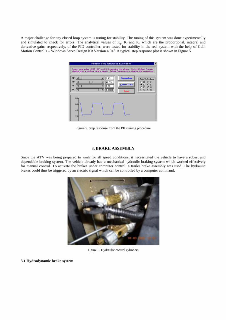
Power amplifier then provides with a signal to generate the required torque. The motor output is geared down to be able

to turn the jeep wheels from extreme left to extreme right in 100 rotations of the motor shaft. For our purpose we use a

gearbox with a gear ratio of 10:1.The gearbox is connected to the steering column as shown in Figure 4 which also

shows the motor, and the steering column.

Figure 4. Photo showing the motor, gearbox and the steering column attached

to the rack and pinion steering mechanism.

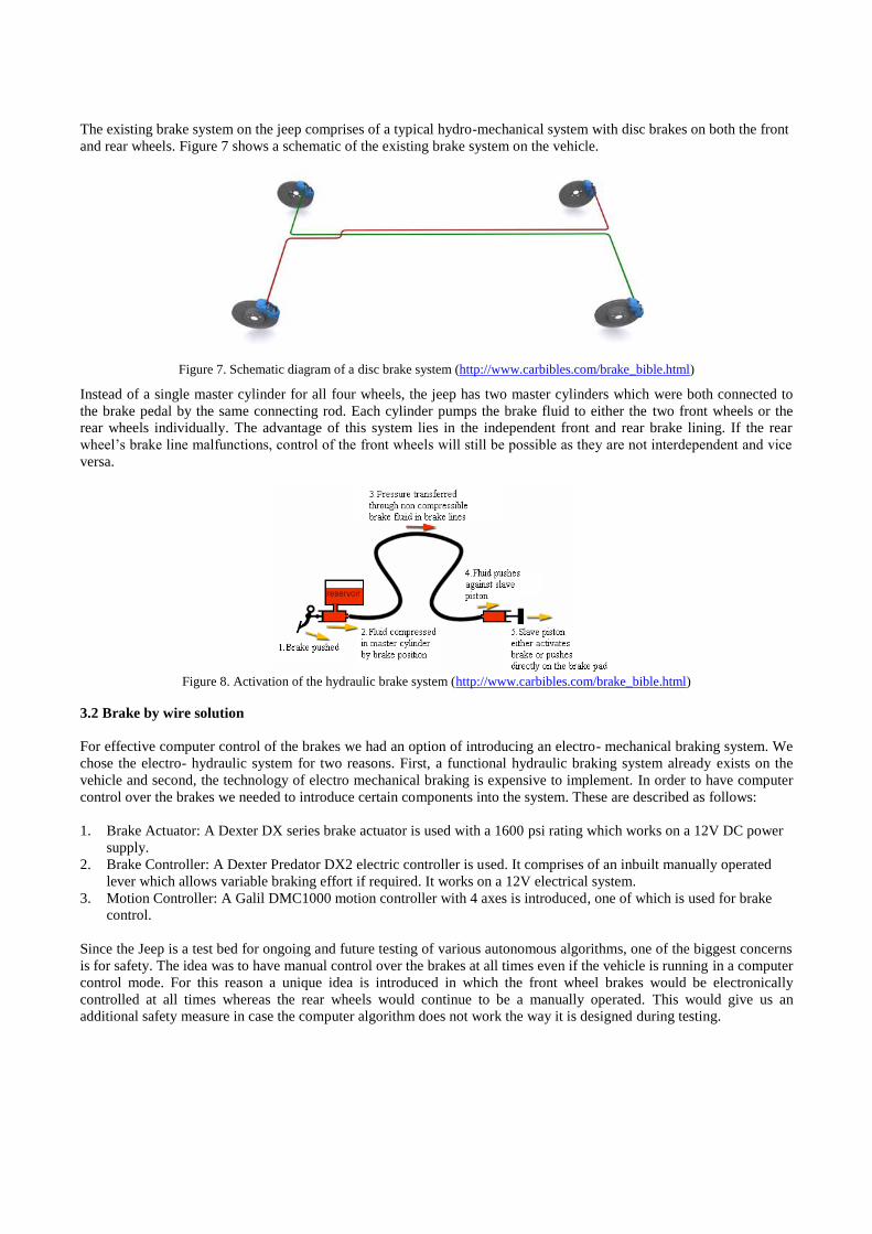
A major challenge for any closed loop system is tuning for stability. The tuning of this system was done experimentally

and simulated to check for errors. The analytical values of Kp, Ki and Kd which are the proportional, integral and

derivative gains respectively, of the PID controller, were tested for stability in the real system with the help of Galil

Motion Control’s – Windows Servo Design Kit Version 4.045. A typical step response plot is shown in Figure 5.

Figure 5. Step response from the PID tuning procedure

3. BRAKE ASSEMBLY

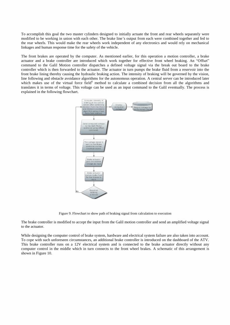
Since the ATV was being prepared to work for all speed conditions, it necessitated the vehicle to have a robust and

dependable braking system. The vehicle already had a mechanical hydraulic braking system which worked effectively

for manual control. To activate the brakes under computer control, a trailer brake assembly was used. The hydraulic

brakes could thus be triggered by an electric signal which can be controlled by a computer command.

Figure 6. Hydraulic control cylinders

3.1 Hydrodynamic brake system

The existing brake system on the jeep comprises of a typical hydro-mechanical system with disc brakes on both the front

and rear wheels. Figure 7 shows a schematic of the existing brake system on the vehicle.

Figure 7. Schematic diagram of a disc brake system (http://www.carbibles.com/brake_bible.html)

Instead of a single master cylinder for all four wheels, the jeep has two master cylinders which were both connected to

the brake pedal by the same connecting rod. Each cylinder pumps the brake fluid to either the two front wheels or the

rear wheels individually. The advantage of this system lies in the independent front and rear brake lining. If the rear

wheel’s brake line malfunctions, control of the front wheels will still be possible as they are not interdependent and vice

versa.

Figure 8. Activation of the hydraulic brake system (http://www.carbibles.com/brake_bible.html)

3.2 Brake by wire solution

For effective computer control of the brakes we had an option of introducing an electro- mechanical braking system. We

chose the electro- hydraulic system for two reasons. First, a functional hydraulic braking system already exists on the

vehicle and second, the technology of electro mechanical braking is expensive to implement. In order to have computer

control over the brakes we needed to introduce certain components into the system. These are described as follows:

1. Brake Actuator: A Dexter DX series brake actuator is used with a 1600 psi rating which works on a 12V DC power

supply.

2. Brake Controller: A Dexter Predator DX2 electric controller is used. It comprises of an inbuilt manually operated

lever which allows variable braking effort if required. It works on a 12V electrical system.

3. Motion Controller: A Galil DMC1000 motion controller with 4 axes is introduced, one of which is used for brake

control.

Since the Jeep is a test bed for ongoing and future testing of various autonomous algorithms, one of the biggest concerns

is for safety. The idea was to have manual control over the brakes at all times even if the vehicle is running in a computer

control mode. For this reason a unique idea is introduced in which the front wheel brakes would be electronically

controlled at all times whereas the rear wheels would continue to be a manually operated. This would give us an

additional safety measure in case the computer algorithm does not work the way it is designed during testing.

To accomplish this goal the two master cylinders designed to initially actuate the front and rear wheels separately were

modified to be working in union with each other. The brake line’s output from each were combined together and fed to

the rear wheels. This would make the rear wheels work independent of any electronics and would rely on mechanical

linkages and human response time for the safety of the vehicle.

The front brakes are operated by the computer. As mentioned earlier, for this operation a motion controller, a brake

actuator and a brake controller are introduced which work together for effective front wheel braking. An “Offset”

command to the Galil Motion controller dispatches a defined voltage signal via the break out board to the brake

controller which is then forwarded to the actuator. The actuator in turn pumps the brake fluid from a reservoir into the

front brake lining thereby causing the hydraulic braking action. The intensity of braking will be governed by the vision,

line following and obstacle avoidance algorithms for the autonomous operation. A central server can be introduced later

which makes use of the virtual force field6 method to calculate a combined decision from all the algorithms and

translates it in terms of voltage. This voltage can be used as an input command to the Galil eventually. The process is

explained in the following flowchart.

Figure 9. Flowchart to show path of braking signal from calculation to execution

The brake controller is modified to accept the input from the Galil motion controller and send an amplified voltage signal

to the actuator.

While designing the computer control of brake system, hardware and electrical system failure are also taken into account.

To cope with such unforeseen circumstances, an additional brake controller is introduced on the dashboard of the ATV.

This brake controller runs on a 12V electrical system and is connected to the brake actuator directly without any

computer control in the middle which in turn connects to the front wheel brakes. A schematic of this arrangement is

shown in Figure 10.

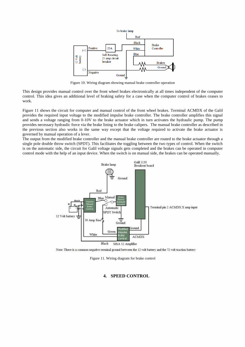
Figure 10. Wiring diagram showing manual brake controller operation

This design provides manual control over the front wheel brakes electronically at all times independent of the computer

control. This idea gives an additional level of braking safety for a case when the computer control of brakes ceases to

work.

Figure 11 shows the circuit for computer and manual control of the front wheel brakes. Terminal ACMDX of the Galil

provides the required input voltage to the modified impulse brake controller. The brake controller amplifies this signal

and sends a voltage ranging from 0-10V to the brake actuator which in turn activates the hydraulic pump. The pump

provides necessary hydraulic force via the brake lining to the brake calipers. The manual brake controller as described in

the previous section also works in the same way except that the voltage required to activate the brake actuator is

governed by manual operation of a lever.

The output from the modified brake controller and the manual brake controller are routed to the brake actuator through a

single pole double throw switch (SPDT). This facilitates the toggling between the two types of control. When the switch

is on the automatic side, the circuit for Galil voltage signals gets completed and the brakes can be operated in computer

control mode with the help of an input device. When the switch is on manual side, the brakes can be operated manually.

Figure 11. Wiring diagram for brake control

4. SPEED CONTROL

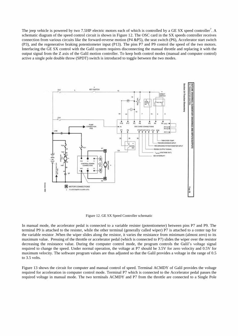
The jeep vehicle is powered by two 7.5HP electric motors each of which is controlled by a GE SX speed controller7. A

schematic diagram of the speed control circuit is shown in Figure 12. The OSC card in the SX speeds controller receives

connection from various circuits like the forward-reverse motion (P4 &P5), the seat switch (P6), Accelerator start switch

(P3), and the regenerative braking potentiometer input (P13). The pins P7 and P9 control the speed of the two motors.

Interfacing the GE SX control with the Galil system requires disconnecting the manual throttle and replacing it with the

output signal from the Z axis of the Galil motion controller. To keep both control modes (manual and computer control)

active a single pole double throw (SPDT) switch is introduced to toggle between the two modes.

Figure 12. GE SX Speed Controller schematic

In manual mode, the accelerator pedal is connected to a variable resister (potentiometer) between pins P7 and P9. The

terminal P9 is attached to the resister, while the other terminal (generally called wiper) P7 is attached to a center tap for

the variable resistor .When the wiper slides along the resistor, it varies the resistance from minimum (almost zero) to its

maximum value. Pressing of the throttle or accelerator pedal (which is connected to P7) slides the wiper over the resistor

decreasing the resistance value. During the computer control mode, the program controls the Galil’s voltage signal

required to change the speed. Under normal operation, the voltage at P7 should be 3.5V for zero velocity and 0.5V for

maximum velocity. The software program values are thus adjusted so that the Galil provides a voltage in the range of 0.5

to 3.5 volts.

Figure 13 shows the circuit for computer and manual control of speed. Terminal ACMDY of Galil provides the voltage

required for acceleration in computer control mode. Terminal P7 which is connected to the Accelerator pedal passes the

required voltage in manual mode. The two terminals ACMDY and P7 from the throttle are connected to a Single Pole

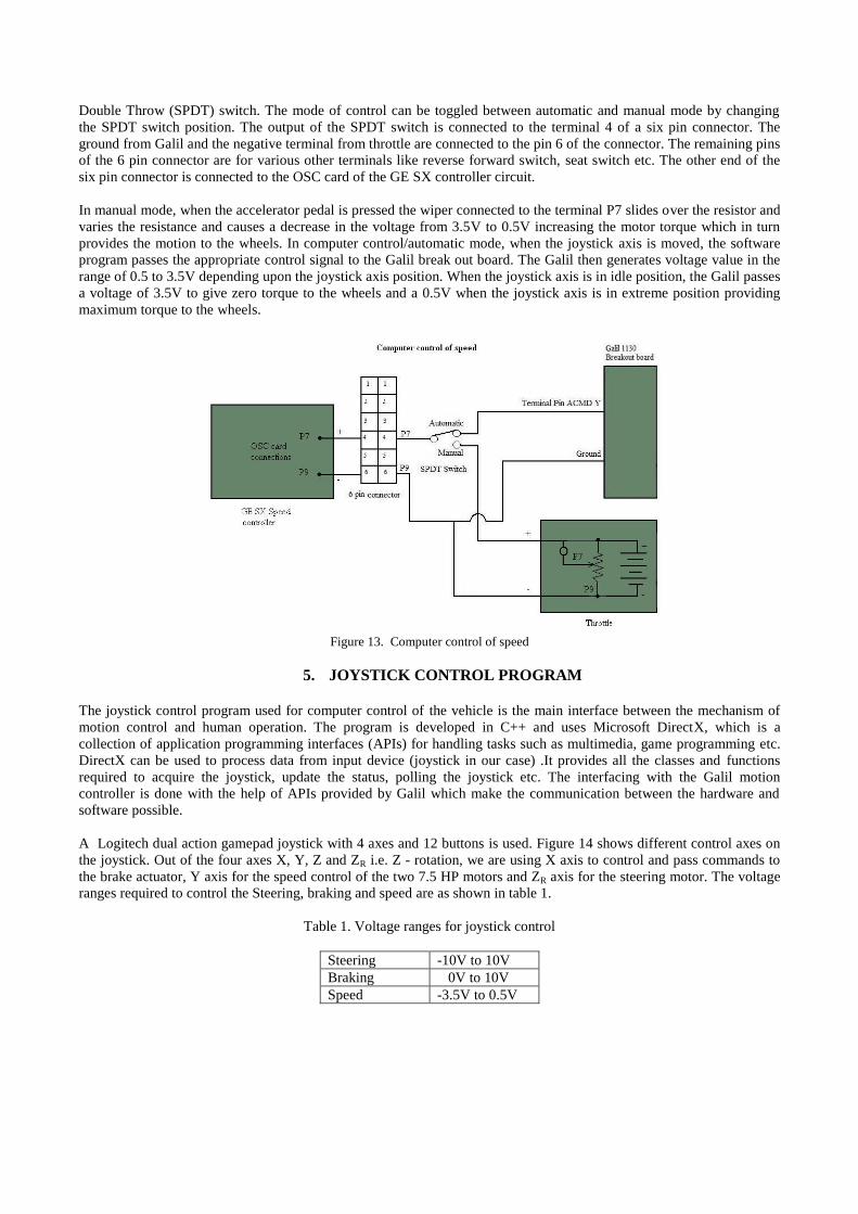
Double Throw (SPDT) switch. The mode of control can be toggled between automatic and manual mode by changing

the SPDT switch position. The output of the SPDT switch is connected to the terminal 4 of a six pin connector. The

ground from Galil and the negative terminal from throttle are connected to the pin 6 of the connector. The remaining pins

of the 6 pin connector are for various other terminals like reverse forward switch, seat switch etc. The other end of the

six pin connector is connected to the OSC card of the GE SX controller circuit.

In manual mode, when the accelerator pedal is pressed the wiper connected to the terminal P7 slides over the resistor and

varies the resistance and causes a decrease in the voltage from 3.5V to 0.5V increasing the motor torque which in turn

provides the motion to the wheels. In computer control/automatic mode, when the joystick axis is moved, the software

program passes the appropriate control signal to the Galil break out board. The Galil then generates voltage value in the

range of 0.5 to 3.5V depending upon the joystick axis position. When the joystick axis is in idle position, the Galil passes

a voltage of 3.5V to give zero torque to the wheels and a 0.5V when the joystick axis is in extreme position providing

maximum torque to the wheels.

Figure 13. Computer control of speed

5. JOYSTICK CONTROL PROGRAM

The joystick control program used for computer control of the vehicle is the main interface between the mechanism of

motion control and human operation. The program is developed in C++ and uses Microsoft DirectX, which is a

collection of application programming interfaces (APIs) for handling tasks such as multimedia, game programming etc.

DirectX can be used to process data from input device (joystick in our case) .It provides all the classes and functions

required to acquire the joystick, update the status, polling the joystick etc. The interfacing with the Galil motion

controller is done with the help of APIs provided by Galil which make the communication between the hardware and

software possible.

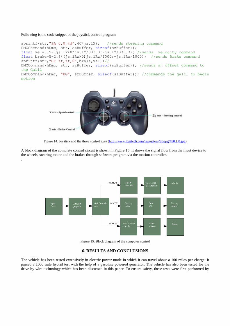
A Logitech dual action gamepad joystick with 4 axes and 12 buttons is used. Figure 14 shows different control axes on

the joystick. Out of the four axes X, Y, Z and ZR i.e. Z - rotation, we are using X axis to control and pass commands to

the brake actuator, Y axis for the speed control of the two 7.5 HP motors and ZR axis for the steering motor. The voltage

ranges required to control the Steering, braking and speed are as shown in table 1.

Table 1. Voltage ranges for joystick control

Steering -10V to 10V

Braking 0V to 10V

Speed -3.5V to 0.5V

Following is the code snippet of the joystick control program

sprintf(str,"PA 0,0,%d",40*js.lX); //sends steering command

DMCCommand(hDmc, str, szBuffer, sizeof(szBuffer));

float vel=3.5-(js.lY>0?js.lY/333.3:-js.lY/333.3); //sends velocity command

float brake=5-2.6*(js.lRz>0?js.lRz/1000:-js.lRz/1000); //sends Brake command

sprintf(str,"OF %f,%f,0",brake,vel);//

DMCCommand(hDmc, str, szBuffer, sizeof(szBuffer)); //sends an offset command to

the Galil

DMCCommand(hDmc, "BG", szBuffer, sizeof(szBuffer)); //commands the galil to begin

motion

Figure 14. Joystick and the three control axes (http://www.logitech.com/repository/95/jpg/450.1.0.jpg)

A block diagram of the complete control circuit is shown in Figure.15. It shows the signal flow from the input device to

the wheels, steering motor and the brakes through software program via the motion controller.

.

Figure 15. Block diagram of the computer control

6. RESULTS AND CONCLUSIONS

The vehicle has been tested extensively in electric power mode in which it can travel about a 100 miles per charge. It

passed a 1000 mile hybrid test with the help of a gasoline powered generator. The vehicle has also been tested for the

drive by wire technology which has been discussed in this paper. To ensure safety, these tests were first performed by

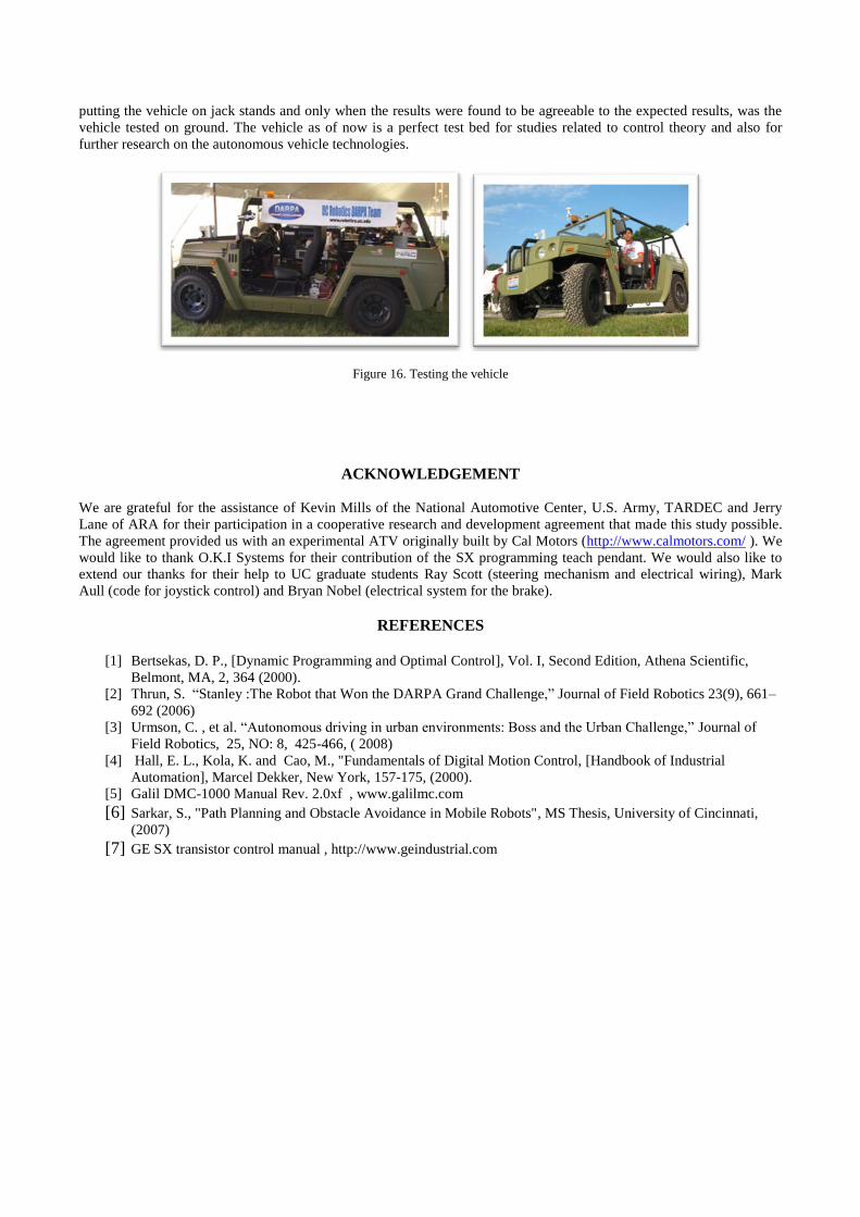
putting the vehicle on jack stands and only when the results were found to be agreeable to the expected results, was the

vehicle tested on ground. The vehicle as of now is a perfect test bed for studies related to control theory and also for

further research on the autonomous vehicle technologies.

Figure 16. Testing the vehicle

ACKNOWLEDGEMENT

We are grateful for the assistance of Kevin Mills of the National Automotive Center, U.S. Army, TARDEC and Jerry

Lane of ARA for their participation in a cooperative research and development agreement that made this study possible.

The agreement provided us with an experimental ATV originally built by Cal Motors (http://www.calmotors.com/ ). We

would like to thank O.K.I Systems for their contribution of the SX programming teach pendant. We would also like to

extend our thanks for their help to UC graduate students Ray Scott (steering mechanism and electrical wiring), Mark

Aull (code for joystick control) and Bryan Nobel (electrical system for the brake).

REFERENCES

[1] Bertsekas, D. P., [Dynamic Programming and Optimal Control], Vol. I, Second Edition, Athena Scientific,

Belmont, MA, 2, 364 (2000).

[2] Thrun, S. “Stanley :The Robot that Won the DARPA Grand Challenge,” Journal of Field Robotics 23(9), 661–

692 (2006)

[3] Urmson, C. , et al. “Autonomous driving in urban environments: Boss and the Urban Challenge,” Journal of

Field Robotics, 25, NO: 8, 425-466, ( 2008)

[4] Hall, E. L., Kola, K. and Cao, M., "Fundamentals of Digital Motion Control, [Handbook of Industrial

Automation], Marcel Dekker, New York, 157-175, (2000).

[5] Galil DMC-1000 Manual Rev. 2.0xf , www.galilmc.com

[6] Sarkar, S., "Path Planning and Obstacle Avoidance in Mobile Robots", MS Thesis, University of Cincinnati,

(2007) [7] GE SX transistor control manual , http://www.geindustrial.com