Le ture NotesOnGeneral RelativityØyvind GrønOslo College, Department of engineering, Cort Adelers gt. 30, N-0254 Oslo,NorwayandDepartment of Physi s, University of Oslo, Box 1048 Blindern, N-0316, Norway

June 6, 2008

Prefa eThese notes are a trans ript of le tures delivered by Øyvind Grøn during thespring of 1997 at the University of Oslo. Two ompendia, (Grøn and Flø 1984)and (Ravndal 1978) were provided by Grøn as additional referen e materialduring the le tures.The present version of this do ument is an extended and orre ted version ofa set of Le ture Notes whi h were typesetted by S. Bard, Andreas O. Jaunsen,Frode Hansen and Ragnvald J. Irgens using LATEX2ǫ. Svend E. Hjelmeland hasmade many useful suggestions whi h have improved the text. I would also like tothank Jon Magne Leinaas and Sigbjørn Hervik for ontributing with problems,and Gorm Krogh Johnsen for help with nishing the manus ript.While we hope that these typeset notes are of benet parti ularly to stu-dents of general relativity and look forward to their omments, we wel ome allinterested readers and a ept all feedba k with thanks.All omment may be sent to the author either by e-mail or snail mail.Øyvind GrønFysisk InstituttUniversitetet i OsloP.O.Boks 1048, Blindern0315 OSLOE-mail: Oyvind.Groniu.hio.no

ContentsList of Figures vList of Denitions ixList of Examples xi1 Newton's law of universal gravitation 11.1 The for e law of gravitation . . . . . . . . . . . . . . . . . . . . . 11.2 Newton's law of gravitation in its lo al form . . . . . . . . . . . . 21.3 Tidal For es . . . . . . . . . . . . . . . . . . . . . . . . . . . . . . 51.4 The Prin iple of Equivalen e . . . . . . . . . . . . . . . . . . . . 91.5 The general prin iple of relativity . . . . . . . . . . . . . . . . . . 101.6 The ovarian e prin iple . . . . . . . . . . . . . . . . . . . . . . . 111.7 Ma h's prin iple . . . . . . . . . . . . . . . . . . . . . . . . . . . 12Problems . . . . . . . . . . . . . . . . . . . . . . . . . . . . . . . . . . 132 The Spe ial Theory of Relativity 172.1 Coordinate systems and Minkowski-diagrams . . . . . . . . . . . 172.2 Syn hronization of lo ks . . . . . . . . . . . . . . . . . . . . . . 192.3 The Doppler ee t . . . . . . . . . . . . . . . . . . . . . . . . . . 192.4 Relativisti time-dilatation . . . . . . . . . . . . . . . . . . . . . . 212.5 The relativity of simultaneity . . . . . . . . . . . . . . . . . . . . 232.6 The Lorentz- ontra tion . . . . . . . . . . . . . . . . . . . . . . . 252.7 The Lorentz transformation . . . . . . . . . . . . . . . . . . . . . 262.8 Lorentz-invariant interval . . . . . . . . . . . . . . . . . . . . . . 292.9 The twin-paradox . . . . . . . . . . . . . . . . . . . . . . . . . . . 312.10 Hyperboli motion . . . . . . . . . . . . . . . . . . . . . . . . . . 322.11 Energy and mass . . . . . . . . . . . . . . . . . . . . . . . . . . . 342.12 Relativisti in rease of mass . . . . . . . . . . . . . . . . . . . . . 362.13 Ta hyons . . . . . . . . . . . . . . . . . . . . . . . . . . . . . . . 362.14 Magnetism as a relativisti se ond-order ee t . . . . . . . . . . . 38Problems . . . . . . . . . . . . . . . . . . . . . . . . . . . . . . . . . . 413 Ve tors, Tensors and Forms 483.1 Ve tors . . . . . . . . . . . . . . . . . . . . . . . . . . . . . . . . 483.1.1 4-ve tors . . . . . . . . . . . . . . . . . . . . . . . . . . . . 49i

3.1.2 Tangent ve tor elds and oordinate ve tors . . . . . . . . 523.1.3 Coordinate transformations . . . . . . . . . . . . . . . . . 553.1.4 Stru ture oe ients . . . . . . . . . . . . . . . . . . . . . 583.2 Tensors . . . . . . . . . . . . . . . . . . . . . . . . . . . . . . . . 603.2.1 Transformation of tensor omponents . . . . . . . . . . . . 623.2.2 Transformation of basis 1-forms . . . . . . . . . . . . . . . 633.2.3 The metri tensor . . . . . . . . . . . . . . . . . . . . . . 633.3 Forms . . . . . . . . . . . . . . . . . . . . . . . . . . . . . . . . . 67Problems . . . . . . . . . . . . . . . . . . . . . . . . . . . . . . . . . . 704 A elerated Referen e Frames 754.1 Rotating referen e frames . . . . . . . . . . . . . . . . . . . . . . 754.1.1 The spatial metri tensor . . . . . . . . . . . . . . . . . . 754.1.2 Angular a eleration in the rotating frame . . . . . . . . . 794.1.3 Gravitational time dilation . . . . . . . . . . . . . . . . . 824.1.4 Path of photons emitted from axes in the rotating refer-en e frame (RF) . . . . . . . . . . . . . . . . . . . . . . . 834.1.5 The Sagna ee t . . . . . . . . . . . . . . . . . . . . . . . 834.2 Hyperboli ally a elerated referen e frames . . . . . . . . . . . . 84Problems . . . . . . . . . . . . . . . . . . . . . . . . . . . . . . . . . . 905 Covariant Dierentiation 955.1 Dierentiation of forms . . . . . . . . . . . . . . . . . . . . . . . . 955.1.1 Exterior dierentiation . . . . . . . . . . . . . . . . . . . . 955.1.2 Covariant derivative . . . . . . . . . . . . . . . . . . . . . 975.2 The Christoel Symbols . . . . . . . . . . . . . . . . . . . . . . . 995.3 Geodesi urves . . . . . . . . . . . . . . . . . . . . . . . . . . . . 1025.4 The ovariant Euler-Lagrange equations . . . . . . . . . . . . . . 1035.5 Appli ation of the Lagrangian formalism to free parti les . . . . . 1055.5.1 Equation of motion from Lagrange's equations . . . . . . 1065.5.2 Geodesi world lines in spa etime . . . . . . . . . . . . . . 1075.5.3 Gravitational Doppler ee t . . . . . . . . . . . . . . . . . 1165.6 The Koszul onne tion . . . . . . . . . . . . . . . . . . . . . . . . 1175.7 Conne tion oe ients Γαµν and stru ture oe ients cαµν in ... . 1205.8 Covariant dierentiation of ve tors, forms and tensors . . . . . . 1215.8.1 Covariant dierentiation of a ve tor in an arbitrary basis . 1215.8.2 Covariant dierentiation of forms . . . . . . . . . . . . . . 1215.8.3 Generalization for tensors of higher rank . . . . . . . . . . 1235.9 The Cartan onne tion . . . . . . . . . . . . . . . . . . . . . . . . 123Problems . . . . . . . . . . . . . . . . . . . . . . . . . . . . . . . . . . 1276 Curvature 1316.1 The Riemann urvature tensor . . . . . . . . . . . . . . . . . . . 1316.2 Dierential geometry of surfa es . . . . . . . . . . . . . . . . . . . 1366.2.1 Surfa e urvature using the Cartan formalism . . . . . . . 1396.3 The Ri i identity . . . . . . . . . . . . . . . . . . . . . . . . . . 140ii

6.4 Bian hi's 1st identity . . . . . . . . . . . . . . . . . . . . . . . . . 1406.5 Bian hi's 2nd identity . . . . . . . . . . . . . . . . . . . . . . . . 141Problems . . . . . . . . . . . . . . . . . . . . . . . . . . . . . . . . . . 1437 Einstein's Field Equations 1477.1 Energy-momentum onservation . . . . . . . . . . . . . . . . . . . 1477.1.1 Newtonian uid . . . . . . . . . . . . . . . . . . . . . . . . 1477.1.2 Perfe t uids . . . . . . . . . . . . . . . . . . . . . . . . . 1497.2 Einstein's urvature tensor . . . . . . . . . . . . . . . . . . . . . . 1497.3 Einstein's eld equations . . . . . . . . . . . . . . . . . . . . . . . 1507.4 The geodesi postulate as a onsequen e of the eld equations . 152Problems . . . . . . . . . . . . . . . . . . . . . . . . . . . . . . . . . . 1538 The S hwarzs hild spa etime 1568.1 S hwarzs hild's exterior solution . . . . . . . . . . . . . . . . . . . 1568.2 Radial free fall in S hwarzs hild spa etime . . . . . . . . . . . . . 1608.3 Light ones in S hwarzs hild spa etime . . . . . . . . . . . . . . . 1628.4 Analyti al extension of the S hwarzs hild oordinates . . . . . . . 1648.5 Embedding of the S hwarzs hild metri . . . . . . . . . . . . . . . 1668.6 De eleration of light . . . . . . . . . . . . . . . . . . . . . . . . . 1668.7 Parti le traje tories in S hwarzs hild 3-spa e . . . . . . . . . . . 1688.7.1 Motion in the equatorial plane . . . . . . . . . . . . . . . 1708.8 Classi al tests of Einstein's general theory of relativity . . . . . . 1728.8.1 The Hafele-Keating experiment . . . . . . . . . . . . . . . 1728.8.2 Mer ury's perihelion pre ession . . . . . . . . . . . . . . . 1748.8.3 Dee tion of light . . . . . . . . . . . . . . . . . . . . . . . 175Problems . . . . . . . . . . . . . . . . . . . . . . . . . . . . . . . . . . 1779 Bla k Holes 1839.1 'Surfa e gravity': gravitational a eleration on the horizon of abla k hole . . . . . . . . . . . . . . . . . . . . . . . . . . . . . . . 1839.2 Hawking radiation:radiation from a bla k hole . . . . . . . . . . . 1849.3 Rotating Bla k Holes: The Kerr metri . . . . . . . . . . . . . . . 1859.3.1 Zero-angular-momentum-observers . . . . . . . . . . . . . 1869.3.2 Does the Kerr spa e have a horizon? . . . . . . . . . . . . 187Problems . . . . . . . . . . . . . . . . . . . . . . . . . . . . . . . . . . 18810 S hwarzs hild's Interior Solution 19510.1 Newtonian in ompressible star . . . . . . . . . . . . . . . . . . . 19510.2 The pressure ontribution to the gravitational mass of a stati ,spheri ally symmetri system . . . . . . . . . . . . . . . . . . . . 19710.3 The Tolman-Oppenheimer-Volkov equation . . . . . . . . . . . . 19810.4 An exa t solution for in ompressible stars - S hwarzs hild's inte-rior solution . . . . . . . . . . . . . . . . . . . . . . . . . . . . . . 200Problems . . . . . . . . . . . . . . . . . . . . . . . . . . . . . . . . . . 201iii

11 Cosmology 20311.1 Comoving oordinate system . . . . . . . . . . . . . . . . . . . . 20311.2 Curvature isotropy - the Robertson-Walker metri . . . . . . . . 20411.3 Cosmi dynami s . . . . . . . . . . . . . . . . . . . . . . . . . . . 20511.3.1 Hubbles law . . . . . . . . . . . . . . . . . . . . . . . . . . 20511.3.2 Cosmologi al redshift of light . . . . . . . . . . . . . . . . 20511.3.3 Cosmi uids . . . . . . . . . . . . . . . . . . . . . . . . . 20711.3.4 Isotropi and homogeneous universe models . . . . . . . . 20811.4 Some osmologi al models . . . . . . . . . . . . . . . . . . . . . . 21111.4.1 Radiation dominated model . . . . . . . . . . . . . . . . . 21111.4.2 Dust dominated model . . . . . . . . . . . . . . . . . . . . 21211.4.3 Transition from radiation- to matter dominated universe . 21611.4.4 Friedmann-Lemaître model . . . . . . . . . . . . . . . . . 21711.5 Inationary Cosmology . . . . . . . . . . . . . . . . . . . . . . . . 22811.5.1 Problems with the Big Bang Models . . . . . . . . . . . . 22811.5.2 Cosmi Ination . . . . . . . . . . . . . . . . . . . . . . . 230Problems . . . . . . . . . . . . . . . . . . . . . . . . . . . . . . . . . . 235Bibliography 243

iv

List of Figures1.1 Newton's law of universal gravitation . . . . . . . . . . . . . . . . 11.2 Newton's law of gravitation in its lo al form . . . . . . . . . . . . 21.3 The denition of solid angle dΩ . . . . . . . . . . . . . . . . . . . 51.4 Tidal For es . . . . . . . . . . . . . . . . . . . . . . . . . . . . . . 61.5 A small Cartesian oordinate system at a distan e R from a massM . . . . . . . . . . . . . . . . . . . . . . . . . . . . . . . . . . . . 71.6 An elasti , ir ular ring falling freely in the Earth's gravitationaleld . . . . . . . . . . . . . . . . . . . . . . . . . . . . . . . . . . 81.7 A tidal for e pendulum . . . . . . . . . . . . . . . . . . . . . . . . 131.8 Photograph of the omet Shoemaker-Levy 9 taken by the Hubble-teles ope, Mar h 1994. . . . . . . . . . . . . . . . . . . . . . . . . 152.1 World-lines . . . . . . . . . . . . . . . . . . . . . . . . . . . . . . 182.2 Clo k syn hronization by the radar method . . . . . . . . . . . . 192.3 The Doppler ee t . . . . . . . . . . . . . . . . . . . . . . . . . . 202.4 Light- lo k . . . . . . . . . . . . . . . . . . . . . . . . . . . . . . 222.5 Moving light- lo k . . . . . . . . . . . . . . . . . . . . . . . . . . 222.6 Simultaneous events A and B. . . . . . . . . . . . . . . . . . . . . 232.7 The simultaneous events of 2.6 in another frame. . . . . . . . . . 242.8 Light ash in a moving train. . . . . . . . . . . . . . . . . . . . . 242.9 Length ontra tion . . . . . . . . . . . . . . . . . . . . . . . . . . 252.10 The interval between A and B is spa e-like, between C and Dlight-like, and between E and F time-like. . . . . . . . . . . . . . 292.11 World-line of an a elerating parti le . . . . . . . . . . . . . . . . 302.12 World-lines of the twin sisters Eva and Elizabeth. . . . . . . . . . 312.13 World line of parti le with onstant rest a eleration. . . . . . . . 332.14 Light pulse in a box. . . . . . . . . . . . . . . . . . . . . . . . . . 342.15 Ta hyon paradox . . . . . . . . . . . . . . . . . . . . . . . . . . . 372.16 Wire seen from its own rest frame. . . . . . . . . . . . . . . . . . 382.17 Wire seen from rest frame of moving harge. . . . . . . . . . . . . 392.18 A Quasar emitting a jet of matter . . . . . . . . . . . . . . . . . . 412.19 Abberation I: Light emitted from a spheri al sour e . . . . . . . . 452.20 Abberation II: View from a far-away observer . . . . . . . . . . . 462.21 Cerenkov radiation from a parti le . . . . . . . . . . . . . . . . . 473.1 Closed polygon (linearly dependent) . . . . . . . . . . . . . . . . 48v

3.2 Carriage at rest (top) and with velo ity ~v (bottom) . . . . . . . . 493.3 World-lines in a Minkowski diagram . . . . . . . . . . . . . . . . 513.4 No position ve tors . . . . . . . . . . . . . . . . . . . . . . . . . . 523.5 Tangentplane . . . . . . . . . . . . . . . . . . . . . . . . . . . . . 523.6 Proper time . . . . . . . . . . . . . . . . . . . . . . . . . . . . . . 553.7 Coordinate transformation, at spa e. . . . . . . . . . . . . . . . 573.8 Basis-ve tors ~e1 and ~e2 . . . . . . . . . . . . . . . . . . . . . . . . 653.9 The ovariant- and ontravariant omponents of a ve tor . . . . . 664.1 Simultaneity in rotating frames . . . . . . . . . . . . . . . . . . . 774.2 Rotating system: Distan e between points on the ir umferen e . 774.3 Rotating system: Dis ontinuity in simultaneity . . . . . . . . . . 784.4 Rotating system: Angular a eleration . . . . . . . . . . . . . . . 804.5 Rotating system: Distan e in rease . . . . . . . . . . . . . . . . . 804.6 Rotating system: Lorentz ontra tion . . . . . . . . . . . . . . . . 814.7 The Sagna ee t . . . . . . . . . . . . . . . . . . . . . . . . . . . 834.8 Hyperboli a eleration . . . . . . . . . . . . . . . . . . . . . . . 854.9 Simultaneity and hyperboli a eleration . . . . . . . . . . . . . . 874.10 The hyperboli ally a elerated referen e system . . . . . . . . . . 895.1 Parallel transport . . . . . . . . . . . . . . . . . . . . . . . . . . . 1015.2 Dierent world-lines onne ting P1 and P2 in a Minkowski diagram1035.3 Geodesi on a at surfa e . . . . . . . . . . . . . . . . . . . . . . 1055.4 Geodesi on a sphere . . . . . . . . . . . . . . . . . . . . . . . . . 1055.5 Timelike geodesi s . . . . . . . . . . . . . . . . . . . . . . . . . . 1075.6 Proje tiles in 3-spa e . . . . . . . . . . . . . . . . . . . . . . . . . 1095.7 Geodesi s in rotating referen e frames . . . . . . . . . . . . . . . 1105.8 Coordinates on a rotating dis . . . . . . . . . . . . . . . . . . . . 1115.9 Proje tiles in a elerated frames . . . . . . . . . . . . . . . . . . . 1125.10 The twin paradox . . . . . . . . . . . . . . . . . . . . . . . . . . 1145.11 Rotating oordinate system . . . . . . . . . . . . . . . . . . . . . 1185.12 Geodesi s in the Poin aré half-plane . . . . . . . . . . . . . . . . 1306.1 Parallel transport of ~A . . . . . . . . . . . . . . . . . . . . . . . . 1316.2 Parallel transport of a ve tor along a triangle of angles 90 isrotated 90 . . . . . . . . . . . . . . . . . . . . . . . . . . . . . . 1326.3 Geometry of parallel transport . . . . . . . . . . . . . . . . . . . 1336.4 Surfa e geometry . . . . . . . . . . . . . . . . . . . . . . . . . . . 1366.5 The tidal for e pendulum . . . . . . . . . . . . . . . . . . . . . . 1458.1 Light ones in S hwarzs hild spa etime . . . . . . . . . . . . . . . 1638.2 Light ones in S hwarzs hild spa etime . . . . . . . . . . . . . . . 1638.3 Embedding of the S hwarzs hild metri . . . . . . . . . . . . . . . 1678.4 De eleration of light . . . . . . . . . . . . . . . . . . . . . . . . . 1678.5 Newtonian entrifugal barrier . . . . . . . . . . . . . . . . . . . . 1718.6 Gravitational ollapse . . . . . . . . . . . . . . . . . . . . . . . . 1728.7 Dee tion of light . . . . . . . . . . . . . . . . . . . . . . . . . . . 175vi

9.1 Stati border and horizon of a Kerr bla k hole . . . . . . . . . . . 18810.1 Hydrostati equilibrium . . . . . . . . . . . . . . . . . . . . . . . 19611.1 S hemati representation of osmologi al redshift . . . . . . . . . 20611.2 Expansion of a radiation dominated universe . . . . . . . . . . . 21211.3 The size of the universe . . . . . . . . . . . . . . . . . . . . . . . 21511.4 Expansion fa tor . . . . . . . . . . . . . . . . . . . . . . . . . . . 21611.5 The expansion fa tor as fun tion of osmi time in units of theage of the universe. . . . . . . . . . . . . . . . . . . . . . . . . . . 22011.6 The Hubble parameter as fun tion of osmi time. . . . . . . . . 22011.7 ....... . . . . . . . . . . . . . . . . . . . . . . . . . . . . . . . . . . 22111.8 The de eleration parameter as fun tion of osmi time. . . . . . . 22211.9 The ratio of the point of time when osmi de elerations turnover to a eleration to the age of the universe. . . . . . . . . . . . 22311.10The osmi red shift of light emitted at the turnover time fromde eleration to a eleration as fun tion of the present relativedensity of va uum energy. . . . . . . . . . . . . . . . . . . . . . . 22411.11The riti al density in units of the onstant density of the va uumenergy as fun tion of time. . . . . . . . . . . . . . . . . . . . . . . 22411.12The relative density of the va uum energy density as fun tion oftime. . . . . . . . . . . . . . . . . . . . . . . . . . . . . . . . . . . 22511.13The density of matter in units of the density of va uum energyas fun tion of time. . . . . . . . . . . . . . . . . . . . . . . . . . . 22511.14The relative density of matter as fun tion of time. . . . . . . . . 22611.15Rate of hange of ΩΛ as fun tion of ln( tt0 ). The value ln( tt0 ) =−40 orresponds to the osmi point of time t0 ∼ 1s. . . . . . . . 22711.16The shape of the potential depends on the sign of µ2. . . . . . . . 23111.17The temperature dependen e of a Higgs potential with a rstorder phase transition. . . . . . . . . . . . . . . . . . . . . . . . . 232

vii

List of Denitions1.2.1 Solid angle . . . . . . . . . . . . . . . . . . . . . . . . . . . . . . . . 43.1.1 4-velo ity . . . . . . . . . . . . . . . . . . . . . . . . . . . . . . . . . 503.1.2 4-momentum . . . . . . . . . . . . . . . . . . . . . . . . . . . . . . . 503.1.3 4-a eleration . . . . . . . . . . . . . . . . . . . . . . . . . . . . . . . 513.1.4 Referen e frame . . . . . . . . . . . . . . . . . . . . . . . . . . . . . . 523.1.5 Coordinate system . . . . . . . . . . . . . . . . . . . . . . . . . . . . 533.1.6 Comoving oordinate system . . . . . . . . . . . . . . . . . . . . . . 533.1.7 Orthonormal basis . . . . . . . . . . . . . . . . . . . . . . . . . . . . 533.1.8 Coordinate basis ve tors. . . . . . . . . . . . . . . . . . . . . . . . . 533.1.9 Coordinate basis ve tors. . . . . . . . . . . . . . . . . . . . . . . . . 563.1.10Orthonormal basis . . . . . . . . . . . . . . . . . . . . . . . . . . . . 573.1.11Commutators between ve tors . . . . . . . . . . . . . . . . . . . . . . 583.1.12Stru ture oe ients cρµν . . . . . . . . . . . . . . . . . . . . . . . . 593.2.1 Multilinear fun tion, tensors . . . . . . . . . . . . . . . . . . . . . . . 613.2.2 Tensor produ t . . . . . . . . . . . . . . . . . . . . . . . . . . . . . . 613.2.3 The metri tensor . . . . . . . . . . . . . . . . . . . . . . . . . . . . . 633.2.4 Contravariant omponents . . . . . . . . . . . . . . . . . . . . . . . . 643.3.1 p-form . . . . . . . . . . . . . . . . . . . . . . . . . . . . . . . . . . . 674.2.1 Born-sti motion . . . . . . . . . . . . . . . . . . . . . . . . . . . . . 865.3.1 Geodesi urves . . . . . . . . . . . . . . . . . . . . . . . . . . . . . . 1025.6.1 Koszul's onne tion oee ients in an arbitrary basis . . . . . . . . . 1185.8.1 Covariant derivative of a ve tor . . . . . . . . . . . . . . . . . . . . . 1215.8.2 Covariant dire tional derivative of a one-form eld . . . . . . . . . . 1215.8.3 Covariant derivative of a one-form . . . . . . . . . . . . . . . . . . . 1225.8.4 Covariant derivative of a tensor . . . . . . . . . . . . . . . . . . . . . 1235.9.1 Exterior derivative of a basis ve tor . . . . . . . . . . . . . . . . . . . 1235.9.2 Conne tion forms Ωνµ . . . . . . . . . . . . . . . . . . . . . . . . . . 1245.9.3 S alar produ t between ve tor and 1-form . . . . . . . . . . . . . . . 1246.5.1 Contra tion . . . . . . . . . . . . . . . . . . . . . . . . . . . . . . . . 1418.1.1 Physi al singularity . . . . . . . . . . . . . . . . . . . . . . . . . . . . 1608.1.2 Coordinate singularity . . . . . . . . . . . . . . . . . . . . . . . . . . 1609.3.1 Horizon . . . . . . . . . . . . . . . . . . . . . . . . . . . . . . . . . . 187

ix

List of Examples3.1.1 Photon lo k . . . . . . . . . . . . . . . . . . . . . . . . . . . . . . . 493.1.2 Coordinate transformation . . . . . . . . . . . . . . . . . . . . . . . . 563.1.3 Relativisti Doppler Ee t . . . . . . . . . . . . . . . . . . . . . . . . 583.1.4 Stru ture oe ients in planar polar oordinates . . . . . . . . . . . 603.2.1 Example of a tensor . . . . . . . . . . . . . . . . . . . . . . . . . . . 623.2.2 A mixed tensor of rank 3 . . . . . . . . . . . . . . . . . . . . . . . . 633.2.3 Cartesian oordinates in a plane . . . . . . . . . . . . . . . . . . . . 643.2.4 Basis-ve tors in plane polar- oordinates . . . . . . . . . . . . . . . . 643.2.5 Non-diagonal basis-ve tors . . . . . . . . . . . . . . . . . . . . . . . . 643.2.6 Cartesian oordinates in a plane . . . . . . . . . . . . . . . . . . . . 663.2.7 Plane polar oordinates . . . . . . . . . . . . . . . . . . . . . . . . . 663.3.1 antisymmetri ombinations . . . . . . . . . . . . . . . . . . . . . . . 673.3.2 antisymmetri ombinations . . . . . . . . . . . . . . . . . . . . . . . 673.3.3 A 2-form in 3-spa e . . . . . . . . . . . . . . . . . . . . . . . . . . . . 685.1.1 Outer produ t of 1-forms in 3-spa e . . . . . . . . . . . . . . . . . . 965.1.2 The derivative of a ve tor eld with rotation . . . . . . . . . . . . . . 985.2.1 The Christoel symbols in plane polar oordinates . . . . . . . . . . 1005.3.1 verti al motion of free parti le in hyperb. a . ref. frame . . . . . . . 1025.5.1 How geodesi s in spa etime an give parabolas in spa e . . . . . . . 1075.5.2 Spatial geodesi s des ribed in the referen e frame of a rotating dis . 1085.5.3 Christoel symbols in a hyperboli ally a elerated referen e frame . 1115.5.4 Verti al proje tile motion in a hyperboli ally a elerated referen eframe . . . . . . . . . . . . . . . . . . . . . . . . . . . . . . . . . . . 1125.5.5 The twin paradox . . . . . . . . . . . . . . . . . . . . . . . . . . . . 1145.5.6 Measurements of gravitational Doppler ee ts (Pound and Rebka 1960)1175.6.1 The onne tion oe ients in a rotating referen e frame. . . . . . . . 1185.6.2 A eleration in a non-rotating referen e frame (Newton) . . . . . . . 1195.6.3 The a eleration of a parti le, relative to the rotating referen e frame 1195.9.1 Cartan- onne tion in an orthonormal basis eld in plane polar oord. 1257.1.1 Energy momentum tensor for a Newtonian uid . . . . . . . . . . . . 14811.4.1Age-redshift relation for dust dominated universe with k = 0 . . . . 214xi

Chapter 1Newton's law of universalgravitation1.1 The for e law of gravitationM

mF

r

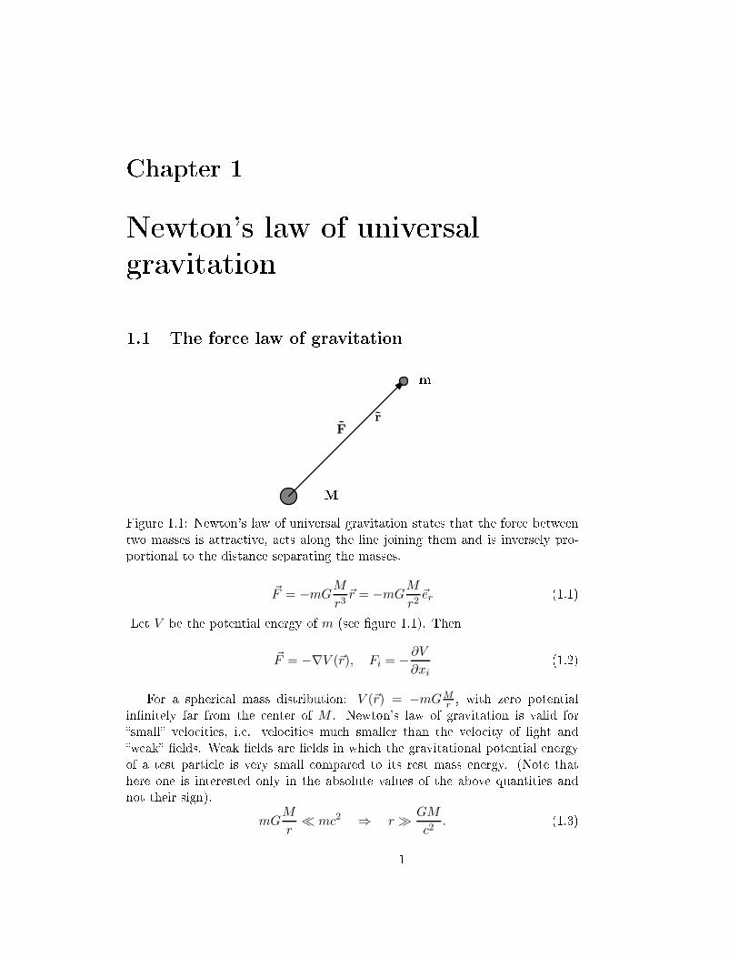
Figure 1.1: Newton's law of universal gravitation states that the for e betweentwo masses is attra tive, a ts along the line joining them and is inversely pro-portional to the distan e separating the masses.~F = −mGM

r3~r = −mGM

r2~er (1.1)Let V be the potential energy of m (see gure 1.1). Then

~F = −∇V (~r), Fi = −∂V∂xi

(1.2)For a spheri al mass distribution: V (~r) = −mGMr , with zero potentialinnitely far from the enter of M . Newton's law of gravitation is valid forsmall velo ities, i.e. velo ities mu h smaller than the velo ity of light andweak elds. Weak elds are elds in whi h the gravitational potential energyof a test parti le is very small ompared to its rest mass energy. (Note thathere one is interested only in the absolute values of the above quantities andnot their sign).

mGM

r≪ mc2 ⇒ r ≫ GM

c2. (1.3)1

2 Chapter 1. Newton's law of universal gravitationThe S hwarzs hild radius for an obje t of mass M is Rs = 2GMc2

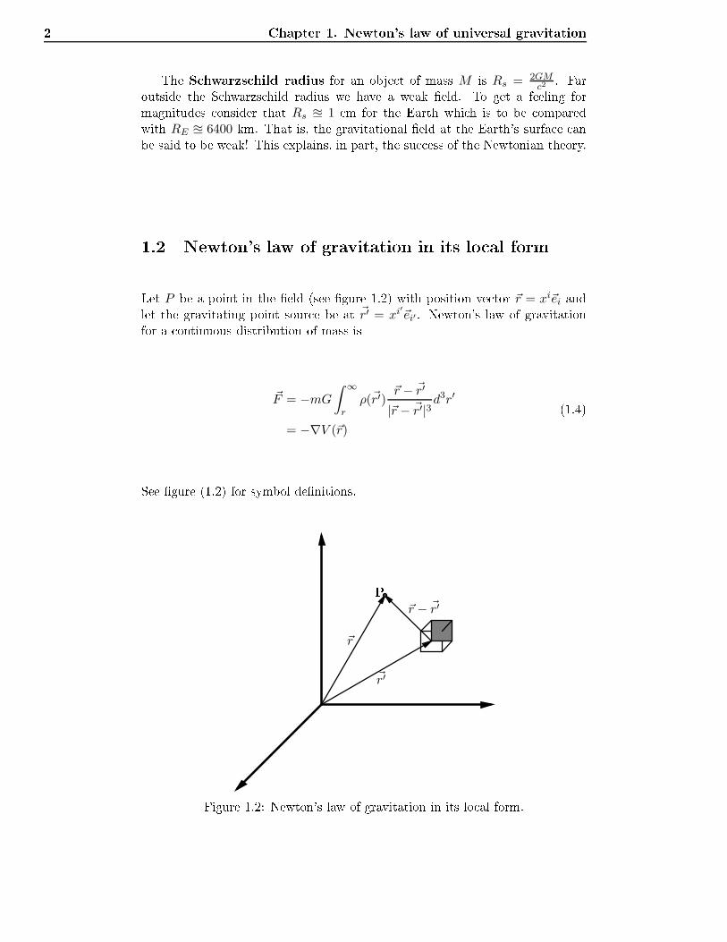
. Faroutside the S hwarzs hild radius we have a weak eld. To get a feeling formagnitudes onsider that Rs ≅ 1 m for the Earth whi h is to be omparedwith RE ≅ 6400 km. That is, the gravitational eld at the Earth's surfa e anbe said to be weak! This explains, in part, the su ess of the Newtonian theory.1.2 Newton's law of gravitation in its lo al formLet P be a point in the eld (see gure 1.2) with position ve tor ~r = xi~ei andlet the gravitating point sour e be at ~r′ = xi

′

~ei′ . Newton's law of gravitationfor a ontinuous distribution of mass is~F = −mG

∫ ∞

rρ(~r′)

~r − ~r′

|~r − ~r′|3d3r′

= −∇V (~r)

(1.4)See gure (1.2) for symbol denitions.

~r′

~r

~r − ~r′P

Figure 1.2: Newton's law of gravitation in its lo al form.

1.2 Newton's law of gravitation in its lo al form 3Let's onsider equation (1.4) term by term.∇ 1

|~r − ~r′|= ~ei

∂

∂xi

1[(xj − xj′)(xj − xj′)

]1/2

= ~ei∂

∂xi

[(xj − xj

′

)(xj − xj′)]−1/2

= ~ei−1

22(xj − xj′)

∂xj

∂xi

[(xk − xk

′

)(xk − xk′)]−3/2

= −~ei(xj − xj

′

)δij

[(xk − xk′)(xk − xk′)]3/2

= −~ei(xi − xi

′

)[(xj − xj′)(xj − xj′)

]3/2

= − ~r − ~r′

|~r − ~r′|3

(1.5)Now equations (1.4) and (1.5) together ⇒

V (~r) = −mG∫

ρ(~r′)

|~r − ~r′|d3r′ (1.6)Gravitational potential at point P :

φ(~r) ≡ V (~r)

m= −G

∫ρ(~r′)

|~r − ~r′|d3r′

⇒ ∇φ(~r) = G

∫ρ(~r′)

~r − ~r′

|~r − ~r′|3d3r′

⇒ ∇2φ(~r) = G

∫ρ(~r′)∇· ~r −

~r′

|~r − ~r′|3d3r′

(1.7)The above equation simplies onsiderably if we al ulate the divergen e in theintegrand. Note that ∇operates on ~ronly!∇· ~r −

~r′

|~r − ~r′|3=

∇·~r|~r − ~r′|3

+ (~r − ~r′) · ∇ 1

|~r − ~r′|3

=3

|~r − ~r′|3− (~r − ~r′) · 3(~r − ~r′)

|~r − ~r′|5

=3

|~r − ~r′|3− 3

|~r − ~r′|3

= 0 ∀ ~r 6= ~r′

(1.8)We on lude that the Newtonian gravitational potential at a point in a gravi-tational eld outside a mass distribution satises Lapla e's equation

∇2φ = 0 (1.9)

4 Chapter 1. Newton's law of universal gravitationDigression 1.2.1 (Dira 's delta fun tion)The Dira delta fun tion has the following properties:1. δ(~r − ~r′) = 0 ∀ ~r 6= ~r′2. ∫ δ(~r − ~r′)d3r′ = 1 when ~r = ~r′ is ontained in the integration domain. Theintegral is identi ally zero otherwise.3. ∫ f(~r′)δ(~r − ~r′)d3r′ = f(~r)A al ulation of the integral ∫ ∇· ~r−~r′|~r−~r′|3d3r′ whi h is valid also in the ase wherethe eld point is inside the mass distribution is obtained through the use ofGauss' integral theorem:

∫v ∇· ~Ad3r′ =

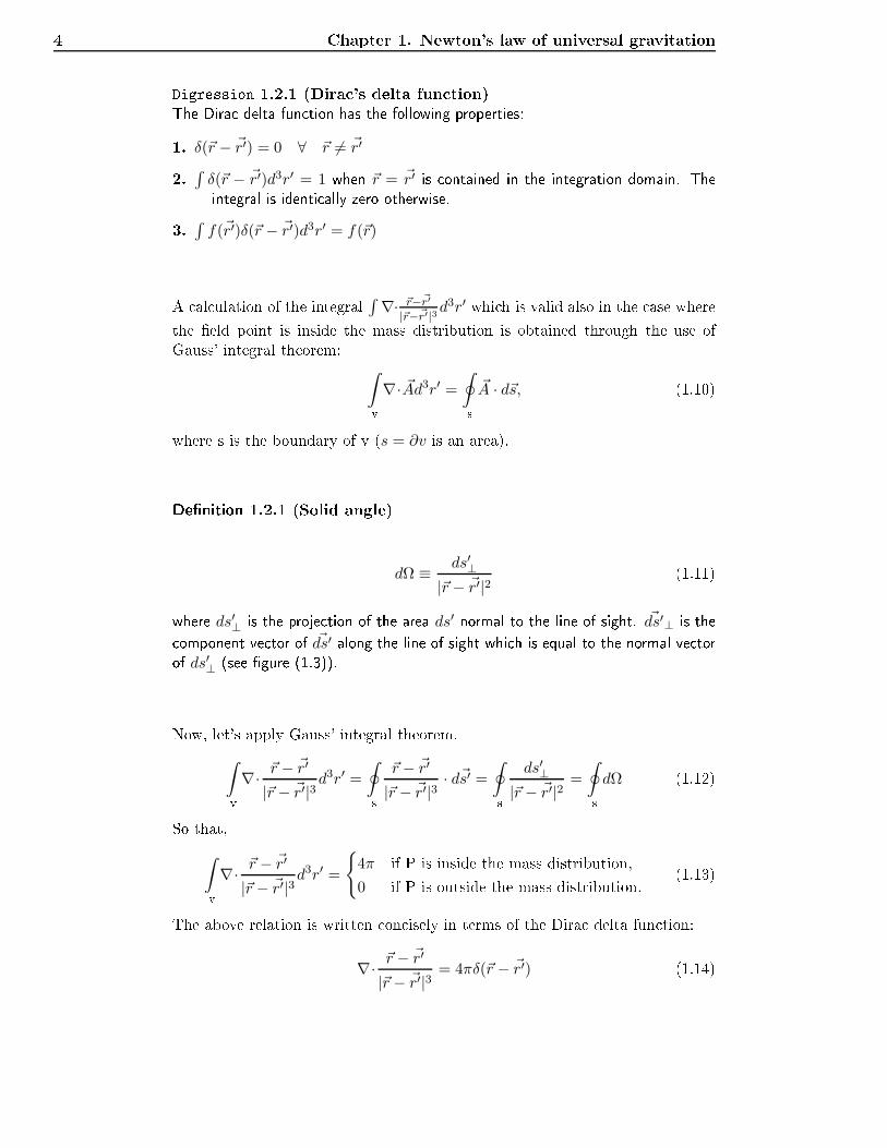
∮s ~A · d~s, (1.10)where s is the boundary of v (s = ∂v is an area).Denition 1.2.1 (Solid angle)dΩ ≡ ds′⊥

|~r − ~r′|2(1.11)where ds′⊥ is the proje tion of the area ds′ normal to the line of sight. ~ds′⊥ is the omponent ve tor of ~ds′ along the line of sight whi h is equal to the normal ve torof ds′⊥ (see gure (1.3)).Now, let's apply Gauss' integral theorem.

∫v ∇· ~r −~r′

|~r − ~r′|3d3r′ =

∮s ~r − ~r′

|~r − ~r′|3· d~s′ =

∮s ds′⊥|~r − ~r′|2

=

∮s dΩ (1.12)So that,∫v ∇· ~r −

~r′

|~r − ~r′|3d3r′ =

4π if P is inside the mass distribution,0 if P is outside the mass distribution. (1.13)The above relation is written on isely in terms of the Dira delta fun tion:∇· ~r −

~r′

|~r − ~r′|3= 4πδ(~r − ~r′) (1.14)

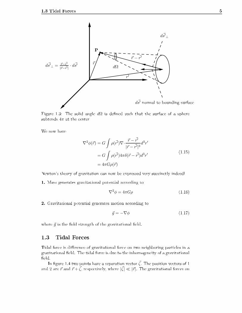
1.3 Tidal For es 5

~r′

~r~r − ~r′

PdΩ

d~s′⊥

d~s′ normal to bounding surfa ed~s′⊥ = ~r−~r′

|~r−~r′| · d~s′

Figure 1.3: The solid angle dΩ is dened su h that the surfa e of a spheresubtends 4π at the enterWe now have∇2φ(~r) = G

∫ρ(~r′)∇· ~r −

~r′

|~r − ~r′|3d3r′

= G

∫ρ(~r′)4πδ(~r − ~r′)d3r′

= 4πGρ(~r)

(1.15)Newton's theory of gravitation an now be expressed very su in tly indeed!1. Mass generates gravitational potential a ording to∇2φ = 4πGρ (1.16)2. Gravitational potential generates motion a ording to~g = −∇φ (1.17)where ~g is the eld strength of the gravitational eld.1.3 Tidal For esTidal for e is dieren e of gravitational for e on two neighboring parti les in agravitational eld. The tidal for e is due to the inhomogeneity of a gravitationaleld.In gure 1.4 two points have a separation ve tor ~ζ. The position ve tors of 1and 2 are ~r and ~r+ ~ζ, respe tively, where |~ζ| ≪ |~r|. The gravitational for es on

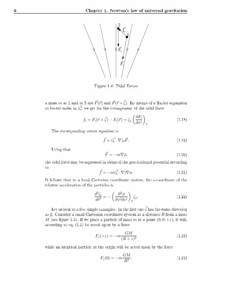
6 Chapter 1. Newton's law of universal gravitationF

F

2

1ζ

1

2

Figure 1.4: Tidal For esa mass m at 1 and at 2 are ~F (~r) and ~F (~r+ ~ζ). By means of a Taylor expansionto lowest order in |~ζ| we get for the i- omponent of the tidal for efi = Fi(~r + ~ζ) − Fi(~r) = ζj

(∂Fi∂xj

)

~r

. (1.18)The orresponding ve tor equation is~f = (~ζ · ∇)~r ~F . (1.19)Using that~F = −m∇φ, (1.20)the tidal for e may be expressed in terms of the gravitational potential a ordingto

~f = −m(~ζ · ∇)∇φ. (1.21)It follows that in a lo al Cartesian oordinate system, the i- oordinate of therelative a eleration of the parti les isd2ζidt2

= −(

∂2φ

∂xi∂xj

)

~r

ζj. (1.22)Let us look at a few simple examples. In the rst one ~ζ has the same dire tionas ~g. Consider a small Cartesian oordinate system at a distan e R from a massM (see gure 1.5). If we pla e a parti le of mass m at a point (0, 0,+z), it will,a ording to eq. (1.1) be a ted upon by a for e

Fz(+z) = −m GM

(R+ z)2(1.23)while an identi al parti le at the origin will be a ted upon by the for e

Fz(0) = −mGM

R2. (1.24)

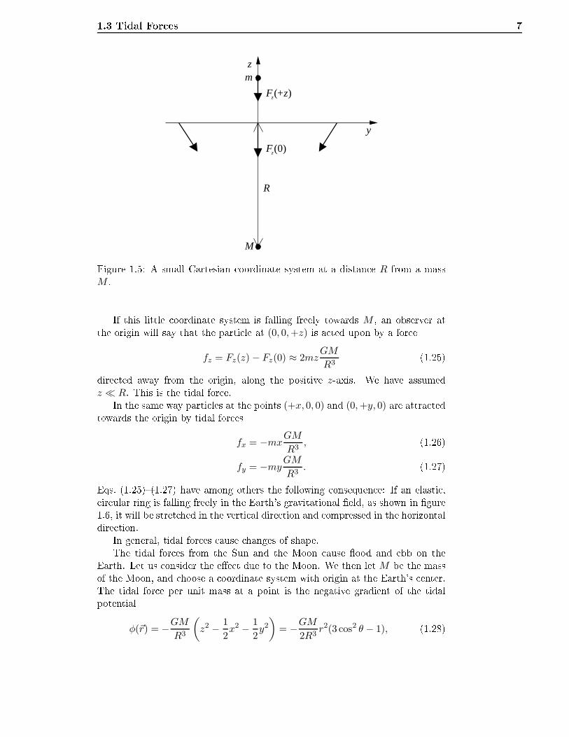
1.3 Tidal For es 7

R

F

F

z

z

(0)

( )+z

m

M

y

z

Figure 1.5: A small Cartesian oordinate system at a distan e R from a massM . If this little oordinate system is falling freely towards M , an observer atthe origin will say that the parti le at (0, 0,+z) is a ted upon by a for e

fz = Fz(z) − Fz(0) ≈ 2mzGM

R3(1.25)dire ted away from the origin, along the positive z-axis. We have assumed

z ≪ R. This is the tidal for e.In the same way parti les at the points (+x, 0, 0) and (0,+y, 0) are attra tedtowards the origin by tidal for esfx = −mxGM

R3, (1.26)

fy = −myGMR3

. (1.27)Eqs. (1.25)(1.27) have among others the following onsequen e: If an elasti , ir ular ring is falling freely in the Earth's gravitational eld, as shown in gure1.6, it will be stret hed in the verti al dire tion and ompressed in the horizontaldire tion.In general, tidal for es ause hanges of shape.The tidal for es from the Sun and the Moon ause ood and ebb on theEarth. Let us onsider the ee t due to the Moon. We then let M be the massof the Moon, and hoose a oordinate system with origin at the Earth's enter.The tidal for e per unit mass at a point is the negative gradient of the tidalpotentialφ(~r) = −GM

R3

(z2 − 1

2x2 − 1

2y2

)= −GM

2R3r2(3 cos2 θ − 1), (1.28)

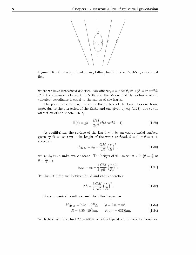
8 Chapter 1. Newton's law of universal gravitation

Figure 1.6: An elasti , ir ular ring falling freely in the Earth's gravitationaleldwhere we have introdu ed spheri al oordinates, z = r cos θ, x2 + y2 = r2 sin2 θ,R is the distan e between the Earth and the Moon, and the radius r of thespheri al oordinate is equal to the radius of the Earth.The potential at a height h above the surfa e of the Earth has one term,mgh, due to the attra tion of the Earth and one given by eq. (1.28), due to theattra tion of the Moon. Thus,

Θ(r) = gh − GM

2R3r2(3 cos2 θ − 1). (1.29)At equilibrium, the surfa e of the Earth will be an equipotential surfa e,given by Θ = onstant. The height of the water at ood, θ = 0 or θ = π, istherefore

hood = h0 +GM

gR

( rR

)2, (1.30)where h0 is an unknown onstant. The height of the water at ebb (θ = π

2 orθ = 3π

2 ) ishebb = h0 −

1

2

GM

gR

( rR

)2. (1.31)The height dieren e between ood and ebb is therefore

∆h =3

2

GM

gR

( rR

)2. (1.32)For a numeri al result we need the following values:

MMoon = 7.35 · 1025g, g = 9.81m/s2, (1.33)R = 3.85 · 105km, rEarth = 6378km. (1.34)With these values we nd ∆h = 53cm, whi h is typi al of tidal height dieren es.

1.4 The Prin iple of Equivalen e 91.4 The Prin iple of Equivalen eGalilei investigated experimentally the motion of freely falling bodies. He foundthat they moved in the same way, regardless what sort of material they onsistedof and what mass they had.In Newton's theory of gravitation mass appears in two dierent ways; asgravitational mass, mG, in the law of gravitation, analogously to harge inCoulomb's law, and as inertial mass, mI in Newton's 2nd law.The equation of motion of a freely falling parti le in the eld of gravity froma spheri al body with mass M then takes the formd2~r

dt2= −GmG

mI

M

r3~r. (1.35)The results of Galilei's measurements imply that the quotient between gravita-tional and inertial mass must be the same for all bodies. With a suitable hoi eof units, we then obtain

mG = mI . (1.36)Measurements performed by the Hungarian baron Eötvös around the turnof the entury indi ated that this equality holds with an a ura y better than10−8. More re ent experiments have given the result |mI

mG− 1| < 9 · 10−13.Einstein assumed the exa t validity of eq.(1.52). He did not onsider this asan a idental oin iden e, but rather as an expression of a fundamental prin iple, alled the prin iple of equivalen e.A onsequen e of this prin iple is the possibility of removing the ee t ofa gravitational for e by being in free fall. In order to larify this, Einstein onsidered a homogeneous gravitational eld in whi h the a eleration of gravity,g, is independent of the position. In a freely falling, non-rotating referen e framein this eld, all free parti les move a ording to

mId2~r

dt2= (mG −mI)~g = 0, (1.37)where eq. (1.36) has been used.This means that an observer in su h a freely falling referen e frame will saythat the parti les around him are not a ted upon by for es. They move with onstant velo ities along straight paths. In other words, su h a referen e frameis inertial.Einstein's heuristi reasoning suggests equivalen e between inertial frames inregions far from mass distributions, where there are no gravitational elds, andinertial frames falling freely in a gravitational eld. This equivalen e between alltypes of inertial frames is so intimately onne ted with the equivalen e betweengravitational and inertial mass, that the term prin iple of equivalen e is usedwhether one talks about masses or inertial frames. The equivalen e of dierenttypes of inertial frames en ompasses all types of physi al phenomena, not onlyparti les in free fall.The prin iple of equivalen e has also been formulated in an opposite way.An observer at rest in a homogeneous gravitational eld, and an observer in

10 Chapter 1. Newton's law of universal gravitationan a elerated referen e frame in a region far from any mass distributions, willobtain identi al results when they perform similar experiments. An inertialeld aused by the a eleration of the referen e frame, is equivalent to a eld ofgravity aused by a mass distribution, as far is tidal ee ts an be ignored.1.5 The general prin iple of relativityThe prin iple of equivalen e led Einstein to a generalization of the spe ial prin i-ple of relativity. In his general theory of relativity Einstein formulated a generalprin iple of relativity, whi h says that not only velo ities are relative, but a el-erations, too.Consider two formulations of the spe ial prin iple of relativity.S1 All laws of Nature are the same (may be formulated in the same way) in allinertial frames.S2 Every inertial observer an onsider himself to be at rest.These two formulations may be interpreted as dierent formulations of asingle prin iple. But the generalization of S1 and S2 to the general ase, whi hen ompasses a elerated motion and non-inertial frames, leads to two dierentprin iples G1 and G2.G1 The laws of Nature are the same in all referen e frames.G2 Every observer an onsider himself to he at rest.In the literature both G1 and G2 are mentioned as the general prin iple ofrelativity. But G2 is a stronger prin iple (i.e. stronger restri tion on naturalphenomena) than G1. Generally the ourse of events of a physi al pro essin a ertain referen e frame, depends upon the laws of physi s, the boundary onditions, the motion of the referen e frame and the geometry of spa e-time.The two latter properties are des ribed by means of a metri al tensor. Byformulating the physi al laws in a metri independent way, one obtains that G1is valid for all types of physi al phenomena.Even if the laws of Nature are the same in all referen e frames, the ourse ofevents of a physi al pro ess will, as mentioned above, depend upon the motionof the referen e frame. As to the spreading of light, for example, the law is thatlight follows null-geodesi urves (see h. 5). This law implies that the path ofa light parti le is urved in non-inertial referen e frames and straight in inertialframes.The question whether G2 is true in the general theory of relativity has beenthoroughly dis ussed re ently, and the answer is not lear yet.

1.6 The ovarian e prin iple 111.6 The ovarian e prin ipleThe prin iple of relativity is a physi al prin iple. It is on erned with physi alphenomena. This prin iple motivates the introdu tion of a formal prin iple, alled the ovarian e prin iple: The equations of a physi al theory shall havethe same form in every oordinate system.This prin iple is not on erned dire tly with physi al phenomena. Theprin iple may be fullled for every theory by writing the equations in a form-invariant i.e. ovariant way. This may he done by using tensor (ve tor) quanti-ties, only, in the mathemati al formulation of the theory.The ovarian e prin iple and the equivalen e prin iple may be used to obtaina des ription of what happens in the presen e of gravitation. We then startwith the physi al laws as formulated in the spe ial theory of relativity. Thenthe laws are written in a ovariant form, by writing them as tensor equations.They are then valid in an arbitrary, a elerated system. But the inertial eld( tive for e) in the a elerated frame is equivalent to a gravitational eld. So,starting with in a des ription referred to an inertial frame, we have obtained ades ription valid in the presen e of a gravitational eld.The tensor equations have in general a oordinate independent form. Yet,su h form-invariant, or ovariant, equations need not fulll the prin iple of rel-ativity.This is due to the following ir umstan es. A physi al prin iple, for examplethe prin iple of relativity, is on erned with observable relationships. Therefore,when one is going to dedu e the observable onsequen es of an equation, onehas to establish relations between the tensor- omponents of the equation andobservable physi al quantities. Su h relations have to be dened; they are notdetermined by the ovarian e prin iple.From the tensor equations, that are ovariant, and the dened relationsbetween the tensor omponents and the observable physi al quantities, one andedu e equations between physi al quantities. The spe ial prin iple of relativity,for example, demands that the laws whi h these equations express must be thesame with referen e to every inertial frameThe relationships between physi al quantities and tensors (ve tors) are the-ory dependent. The relative velo ity between two bodies, for example, is ave tor within Newtonian kinemati s. However, in the relativisti kinemati s offour-dimensional spa e-time, an ordinary velo ity, whi h has only three om-ponents, is not a ve tor. Ve tors in spa e-time, so alled 4-ve tors, have four omponents. Equations between physi al quantities are not ovariant in general.For example, Maxwell's equations in three-ve tor-form are not invariant un-der a Galilei transformation. However, if these equations are rewritten in tensor-form, then neither a Galilei transformation nor any other transformation will hange the form of the equations.If all equations of a theory are tensor equations, the theory is said to be givena manifestly ovariant form. A theory that is written in a manifestly ovariantform, will automati ally fulll the ovarian e prin iple, but it need not fulllthe prin iple of relativity.

12 Chapter 1. Newton's law of universal gravitation1.7 Ma h's prin ipleEinstein gave up Newton's idea of an absolute spa e. A ording to Einstein allmotion is relative. This may sound simple, but it leads to some highly non-trivialand fundamental questions.Imagine that there are only two parti les onne ted by a spring, in theuniverse. What will happen if the two parti les rotate about ea h other? Willthe spring be stret hed due to entrifugal for es? Newton would have onrmedthat this is indeed what will happen. However, when there is no longer anyabsolute spa e that the parti les an rotate relatively to, the answer is not soobvious. If we, as observers, rotate around the parti les, and they are at rest,we would not observe any stret hing of the spring. But this situation is nowkinemati ally equivalent to the one with rotating parti les and observers at rest,whi h leads to stret hing.Su h problems led Ma h to the view that all motion is relative. The motionof a parti le in an empty universe is not dened. All motion is motion relativelyto something else, i.e. relatively to other masses. A ording to Ma h this impliesthat inertial for es must be due to a parti le's a eleration relatively to the greatmasses of the universe. If there were no su h osmi masses, there would notexist inertial for es, like the entrifugal for e. In our example with two parti les onne ted by a string, there would not be any stret hing of the spring, if therewere no osmi masses that the parti les ould rotate relatively to.Another example may be illustrated by means of a turnabout. If we stayon this, while it rotates, we feel that the entrifugal for es lead us outwards.At the same time we observe that the heavenly bodies rotate. A ording toMa h identi al entrifugal for es should appear if the turnabout is stati andthe heavenly bodies rotate.Einstein was strongly inuen ed by Ma h's arguments, whi h probably hadsome inuen e, at least with regards to motivation, on Einstein's onstru tionof his general theory of relativity. Yet, it is lear that general relativity does notfulll all requirements set by Ma h's prin iple. For example there exist generalrelativisti , rotating osmologi al models, where free parti les will tend to rotaterelative to the osmi masses of the model.However, some Ma hian ee ts have been shown to follow from the equationsof the general theory of relativity. For example, inside a rotating, massiveshell the inertial frames, i.e. the free parti les, are dragged on and tend torotate in the same dire tion as the shell. This was dis overed by Lense andThirring in 1918 and is therefore alled the Lense-Thirring ee t. More re entinvestigations of this ee t have, among others, lead to the following result (Brilland Cohen 1966): A massive shell with radius equal to its S hwarzs hild radiushas often been used as an idealized model of our universe. Our result showsthat in su h models lo al inertial frames near the enter annot rotate relativelyto the mass of the universe. In this way our result gives an explanation ina ordan e with Ma h's prin iple, of the fa t that the xed stars is at rest onheaven as observed from an inertial referen e frame.

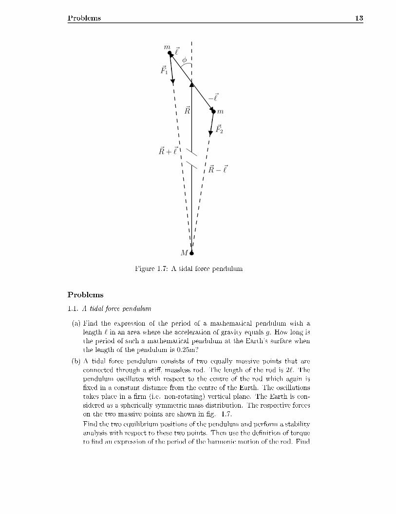
Problems 13

~R − ~ℓ

φ

~R

M

~F2

~F1

m

m

~ℓ

−~ℓ

~R + ~ℓ

Figure 1.7: A tidal for e pendulumProblems1.1. A tidal for e pendulum(a) Find the expression of the period of a mathemati al pendulum with alength ℓ in an area where the a eleration of gravity equals g. How long isthe period of su h a mathemati al pendulum at the Earth's surfa e whenthe length of the pendulum is 0.25m?(b) A tidal for e pendulum onsists of two equally massive points that are onne ted through a sti, massless rod. The length of the rod is 2ℓ. Thependulum os illates with respe t to the entre of the rod whi h again isxed in a onstant distan e from the entre of the Earth. The os illationstakes pla e in a rm (i.e. non-rotating) verti al plane. The Earth is on-sidered as a spheri ally symmetri mass distribution. The respe tive for eson the two massive points are shown in g. 1.7.Find the two equilibrium positions of the pendulum and perform a stabilityanalysis with respe t to these two points. Then use the denition of torqueto nd an expression of the period of the harmoni motion of the rod. Find

14 Chapter 1. Newton's law of universal gravitationthe period at the surfa e of the Earth. Is it possible to hava a similarharmoni motion in a homogenous gravitational eld?1.2. Newtonian potentials for spheri ally symmetri bodies(a) Cal ulate the Newtonian potential φ(r) for a spheri al shell of matter.Assume that the thi kness of the shell is negligible, and the mass per unitarea, σ, is onstant on the spheri al shell. Find the potential both insideand outside the shell.(b) Let R and M be the radius and the mass of the Earth. Find the potentialφ(r) for r < R and r > R. The mass-density is assumed to be onstantfor r < R. Cal ulate the gravitational a eleration on the surfa e of theEarth. Compare with the a tual value of g = 9.81m/s2 (M = 6.0 · 1024kgand R = 6.4 · 106m).( ) Assume that a hollow tube has been drilled right through the entre of theEarth. A small solid ball is then dropped into the tube from the surfa eof the Earth. Find the position of the ball as a fun tion of time. What isthe period of the os illations of the ball?(d) We now assume that the tube is not passing through the entre of theEarth, but at a losest distan e s from the entre. Find how the period ofthe os illations vary as a fun tion of s. Assume for simpli ity that the ballis sliding without fri tion (i.e. no rotation) in the tube.1.3. The Earth-Moon system(a) Assume that the Earth and the Moon are point obje ts and isolated fromthe rest of the Solar system. Put down the equations of motion for theEarth-Moon system. Show that there is a solution where the Earth andMoon are moving in perfe t ir ular orbits around their ommon entre ofmass. What is the radii of the orbits when we know the mass of the Earthand the Moon, and the orbital period of the Moon?(b) Find the Newtonian potential along the line onne ting the two bodies.Draw the result in a plot, and nd the point on the line where the gravi-tational intera tions from the bodies exa tly an el ea h other.( ) The Moon a ts with a dierent for e on a 1 kilogram measure on the surfa eof Earth, depending on whether it is losest to or farthest from the Moon.Find the dieren e in these for es.1.4. The Ro he-limit(a) A spheri al moon with a mass m and radius R is orbiting a planet withmass M . Show that if the moon is loser to its parent planet's entre than

r =

(2M

m

)1/3

R,then loose ro ks on the surfa e of the moon will be elevated due to tidalee ts.

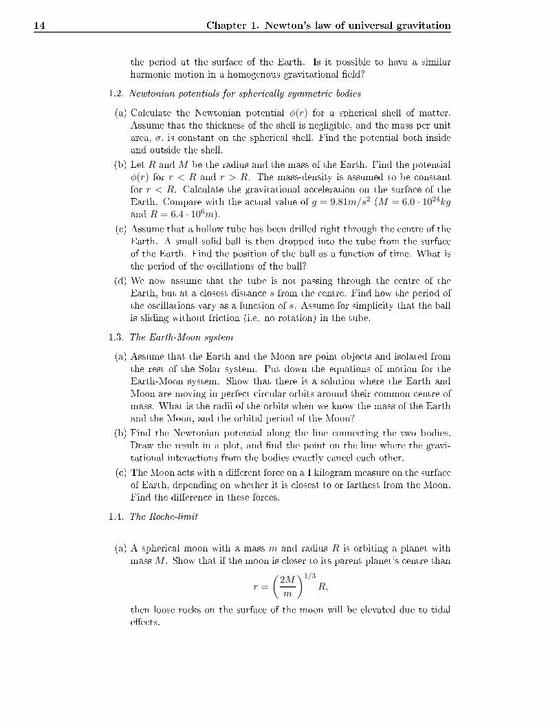
Problems 15

Figure 1.8: Photograph of the omet Shoemaker-Levy 9 taken by the Hubble-teles ope, Mar h 1994.(b) The omet Shoemaker-Levy 9, that in July 1994 ollided with Jupiter, wasripped apart already in 1992 after having passed near Jupiter. Assumingthe omet had a mass of m = 2, 0 · 1012 kg and that the losest passingin 1992 was at a distan e of 96000 km from the entre of Jupiter, it ispossible to estimate the size of the omet. Use that the mass of Jupiter isM = 1, 9 · 1027 kg.1.5. The strength of gravity ompared to the Coulomb for e(a) Determine the dieren e in strength between the Newtonian gravitationalattra tion and the Coulomb for e of the intera tion of the proton and theele tron in a hydrogen atom.(b) What is the gravitational for e of attra tion of two obje ts of 1kg at aseparation of 1m. Compare with the orresponding ele trostati for e oftwo harges of 1C at the same distan e.( ) Compute the gravitational for e between the Earth and the Sun. If the at-tra tive for e was not gravitational but aused by opposite ele tri harges,then what would the harges be?1.6. Falling obje ts in the gravitational eld of the Earth(a) Two test parti les are in free fall towards the entre of the Earth. Theyboth start from rest at a height of 3 Earth radii and with a horizontalseparation of 1m. How far have the parti les fallen when the distan ebetween them is redu ed to 0.5m?(b) Two new test parti les are dropped from the same height with a timeseparation of 1s. The rst parti le is dropped from rest. The se ondparti le is given an initial velo ity equal to the instantaneous velo ity ofthe rst parti le, and it follows after the rst one in the same traje tory.How far and how long have the parti les fallen when the distan e betweenthem is doubled?1.7. A Newtonian Bla k HoleIn 1783 the English physi ist John Mi hell used Newtonian dynami s and lawsof gravity to show that for massive bodies whi h were small enough, the es ape

16 Chapter 1. Newton's law of universal gravitationvelo ity of the bodies are larger than the speed of light. (The same was empha-sized by the Fren h mathemati ian and astronomer Pierre Lapla e in 1796).(a) Assume that the body is spheri al with mass M . Find the largest radius,R, that the body an have in order for it to be a Bla k Hole, i.e. sothat light annot es ape. Assume naively that photons have kineti energy12mc

2.(b) Find the tidal for e on two bodies m at the surfa e of a spheri al body,when their internal distan e is ζ. What would the tidal for e be on thehead and the feet of a 2m tall human, standing upright, in the following ases ( onsider the head and feet as point parti les, ea h weighing 5kg):1. The human is standing on the surfa e of a Bla k Hole with 10 times theSolar mass.2. On the Sun's surfa e.3. On the Earth's surfa e.

Chapter 2The Spe ial Theory of RelativityIn this hapter we shall give a short introdu tion to to the fundamental prin iplesof the spe ial theory of relativity, and dedu e some of the onsequen es of thetheory.The spe ial theory of relativity was presented by Albert Einstein in 1905. Itwas founded on two postulates:1. The laws of physi s are the same in all Galilean frames.2. The velo ity of light in empty spa e is the same in all Galilean frames andindependent of the motion of the light sour e.Einstein pointed out that these postulates are in oni t with Galilean kinemat-i s, in parti ular with the Galilean law for addition of velo ities. A ording toGalilean kinemati s two observers moving relative to ea h other annot measurethe same velo ity for a ertain light signal. Einstein solved this problem by athorough dis ussion of how two distant lo ks should be syn hronized.2.1 Coordinate systems and Minkowski-diagramsThe most simple physi al phenomenon that we an des ribe is alled an event.This is an in ident that takes pla e at a ertain point in spa e and at a ertainpoint in time. A typi al example is the ash from a ashbulb.A omplete des ription of an event is obtained by giving the position of theevent in spa e and time. Assume that our observations are made with referen eto a referen e frame. We introdu e a oordinate system into our referen e frame.Usually it is advantageous to employ a Cartesian oordinate system. This maybe thought of as a ubi latti e onstru ted by measuring rods. If one latti epoint is hosen as origin, with all oordinates equal to zero, then any otherlatti e point has three spatial oordinates equal to the distan es of that pointalong the oordinate axes that pass through the origin. The spatial oordinatesof an event are the three oordinates of the latti e point at whi h the eventhappens.It is somewhat more di ult to determine the point of time of an event. Ifan observer is sitting at the origin with a lo k, then the point of time when17

18 Chapter 2. The Spe ial Theory of Relativityhe at hes sight of an event is not the point of time when the event happened.This is be ause the light takes time to pass from the position of the event tothe observer at the origin. Sin e observers at dierent positions have to makedierent su h orre tions, it would be simpler to have (imaginary) observers atea h point of the referen e frame su h that the point of time of an arbitraryevent an be measured lo ally.But then a new problem appears. One has to syn hronize the lo ks, sothat they show the same time and go at the same rate. This may be performedby letting the observer at the origin send out light signals so that all the other lo ks an be adjusted (with orre tion for light-travel time) to show the sametime as the lo k at the origin. These lo ks show the oordinate time of the oordinate system, and they are alled oordinate lo ks.By means of the latti e of measuring rods and oordinate lo ks, it is noweasy to determine four oordinates (x0 = ct, x, y, z) for every event. (We havemultiplied the time oordinate t by the velo ity of light c in order that all four oordinates shall have the same dimension.)This oordinatization makes it possible to des ribe an event as a point Pin a so- alled Minkowski-diagram. In this diagram we plot ct along the verti alaxis and one of the spatial oordinates along the horizontal axis.In order to observe parti les in motion, we may imagine that ea h parti leis equipped with a ash-light, and that they ash at a onstant frequen y. Theashes from a parti le represent a su ession of events. If they are plotted intoa Minkowski-diagram, we get a series of points that des ribe a urve in the ontinuous limit. Su h a urve is alled a world-line of the parti le. The world-line of a free parti le is a straight line, as shown to left of the time axis in g2.1.x

tlight- onelight- one

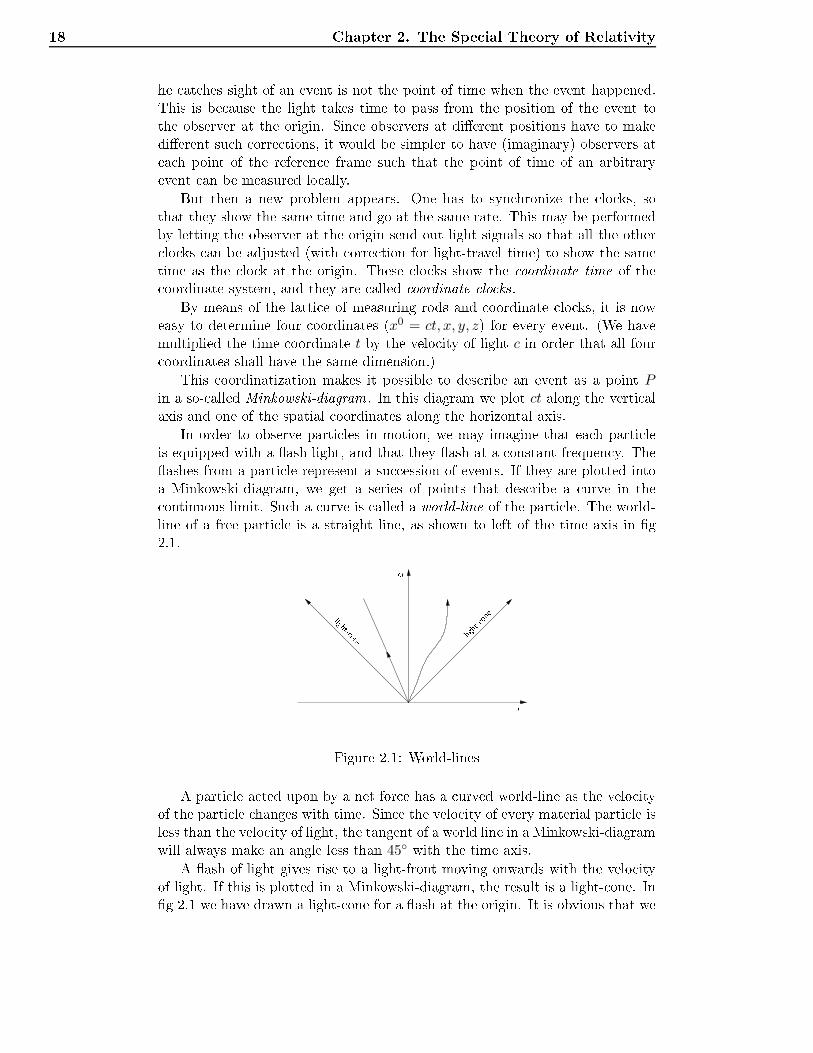
Figure 2.1: World-linesA parti le a ted upon by a net for e has a urved world-line as the velo ityof the parti le hanges with time. Sin e the velo ity of every material parti le isless than the velo ity of light, the tangent of a world line in a Minkowski-diagramwill always make an angle less than 45 with the time axis.A ash of light gives rise to a light-front moving onwards with the velo ityof light. If this is plotted in a Minkowski-diagram, the result is a light- one. Ing 2.1 we have drawn a light- one for a ash at the origin. It is obvious that we

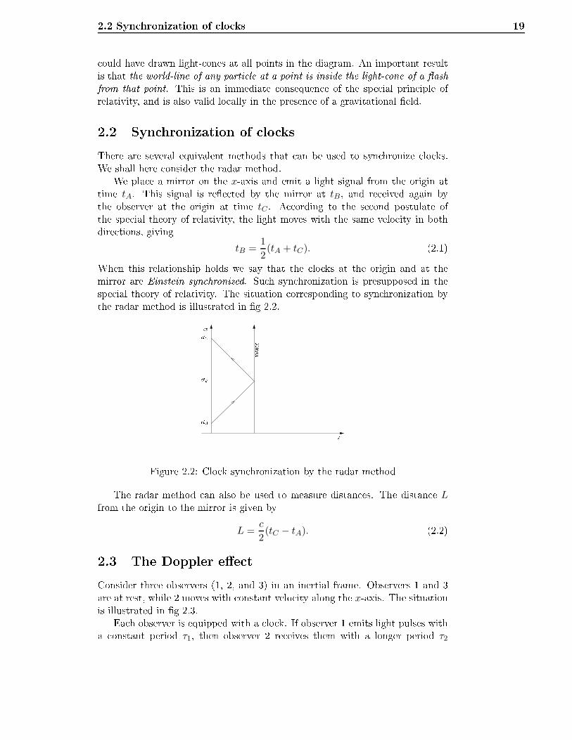
2.2 Syn hronization of lo ks 19 ould have drawn light- ones at all points in the diagram. An important resultis that the world-line of any parti le at a point is inside the light- one of a ashfrom that point. This is an immediate onsequen e of the spe ial prin iple ofrelativity, and is also valid lo ally in the presen e of a gravitational eld.2.2 Syn hronization of lo ksThere are several equivalent methods that an be used to syn hronize lo ks.We shall here onsider the radar method.We pla e a mirror on the x-axis and emit a light signal from the origin attime tA. This signal is ree ted by the mirror at tB, and re eived again bythe observer at the origin at time tC . A ording to the se ond postulate ofthe spe ial theory of relativity, the light moves with the same velo ity in bothdire tions, givingtB =

1

2(tA + tC). (2.1)When this relationship holds we say that the lo ks at the origin and at themirror are Einstein syn hronized. Su h syn hronization is presupposed in thespe ial theory of relativity. The situation orresponding to syn hronization bythe radar method is illustrated in g 2.2.

x

t Mirror tB tA

tC

Figure 2.2: Clo k syn hronization by the radar methodThe radar method an also be used to measure distan es. The distan e Lfrom the origin to the mirror is given byL =

c

2(tC − tA). (2.2)2.3 The Doppler ee tConsider three observers (1, 2, and 3) in an inertial frame. Observers 1 and 3are at rest, while 2 moves with onstant velo ity along the x-axis. The situationis illustrated in g 2.3.Ea h observer is equipped with a lo k. If observer 1 emits light pulses witha onstant period τ1, then observer 2 re eives them with a longer period τ2

20 Chapter 2. The Spe ial Theory of Relativity

x

t 2 31

xB tB tA tC BA

C

Figure 2.3: The Doppler ee ta ording to his or her1 lo k. The fa t that these two periods are dierent is awell-known phenomenon, alled the Doppler ee t . The same ee t is observedwith sound; the tone of a re eding vehi le is lower than that of an approa hingone.We are now going to dedu e a relativisti expression for the Doppler ee t.Firstly, we see from g 2.3 that the two periods τ1 and τ2 are proportional toea h other,τ2 = Kτ1. (2.3)The onstant K(v) is alled Bondi's K-fa tor. Sin e observer 3 is at rest, theperiod τ3 is equal to τ1 so thatτ3 =

1

Kτ2. (2.4)These two equations imply that if 2 moves away from 1, so that τ2 > τ1, then

τ3 < τ2. This is be ause 2 moves towards 3.The K-fa tor is most simply determined by pla ing observer 1 at the origin,while letting the lo ks show t1 = t2 = 0 at the moment when 2 passes theorigin. This is done in g 2.3. The light pulse emitted at the point of time tA,is re eived by 2 when his lo k shows τ2 = KtA. If 2 is equipped with a mirror,the ree ted light pulse is re eived by 1 at a point of time tC = Kτ2 = K2tA.A ording to Eq. (2.1) the ree tion-event then happens at a point of timetB =

1

2(tC + tA) =

1

2(K2 + 1)tA. (2.5)The mirror has then arrived at a distan e xB from the origin, given by Eq. (2.2),

xB =c

2(tC − tA) =

c

2(K2 − 1)tA. (2.6)1For simpli ity we shallwithout any sexist impli ationsfollow the grammati al onven-tion of using mas uline pronouns, instead of the more umbersome `his or her'.

2.4 Relativisti time-dilatation 21Thus, the velo ity of observer 2 isv =

xBtB

= cK2 − 1

K2 + 1. (2.7)Solving this equation with respe t to the K-fa tor we get

K =

(c+ v

c− v

)1/2

. (2.8)This result is relativisti ally orre t. The spe ial theory of relativity was in- luded through the ta it assumption that the velo ity of the ree ted light is c.This is a onsequen e of the se ond postulate of spe ial relativity; the velo ityof light is isotropi and independent of the velo ity of the light sour e.Sin e the wavelength λ of the light is proportional to the period τ , Eq. (2.3)gives the observed wavelength λ′ for the ase when the observer moves awayfrom the sour e,λ′ = Kλ =

(c+ v

c− v

)1/2

λ. (2.9)This Doppler-ee t represents a red-shift of the light. If the light sour e movestowards the observer, there is a orresponding blue-shift given by K−1.It is ommon to express this ee t in terms of the relative hange of wave-length,z =

λ′ − λ

λ= K − 1 (2.10)whi h is positive for red-shift. If v ≪ c, Eq. (2.9) gives,

λ′

λ= K ≈ 1 +

v

c(2.11)to lowest order in v/c. The red-shift is then

z =v

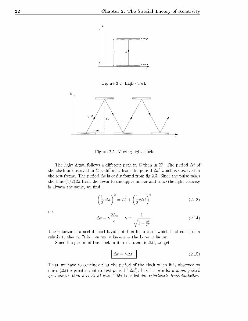
c. (2.12)This result is well known from non-relativisti physi s.2.4 Relativisti time-dilatationEvery periodi motion an be used as a lo k. A parti ularly simple lo k is alled the light lo k. This is illustrated in g 2.4.The lo k onsists of two parallel mirrors that ree t a light pulse ba k andforth. If the period of the lo k is dened as the time interval between ea htime the light pulse hits the lower mirror, then ∆t′ = 2L0/c.Assume that the lo k is at rest in an inertial referen e frame Σ′ where itis pla ed along the y-axis, as shown in g 2.4. If this system moves along the

ct-axis with a velo ity v relative to another inertial referen e frame Σ, the lightpulse of the lo k will follow a zigzag path as shown in g 2.5.

22 Chapter 2. The Spe ial Theory of Relativity

x0

y00

MirrorL0 MirrorFigure 2.4: Light- lo k

x

y

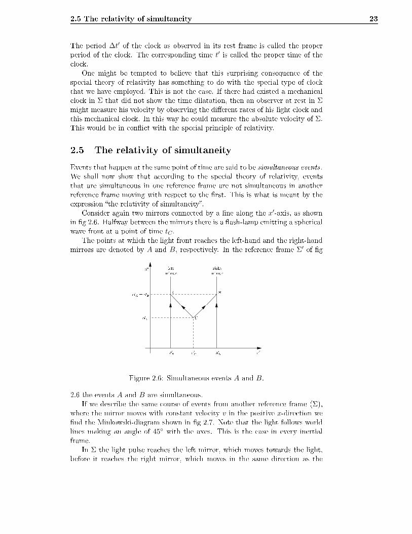
12 t L012vtFigure 2.5: Moving light- lo kThe light signal follows a dierent path in Σ than in Σ′. The period ∆t ofthe lo k as observed in Σ is dierent from the period ∆t′ whi h is observed inthe rest frame. The period ∆t is easily found from g 2.5. Sin e the pulse takesthe time (1/2)∆t from the lower to the upper mirror and sin e the light velo ityis always the same, we nd

(1

2c∆t

)2

= L20 +

(1

2v∆t

)2 (2.13)i.e.∆t = γ

2L0

c, γ ≡ 1√

1 − v2

c2

. (2.14)The γ fa tor is a useful short-hand notation for a term whi h is often used inrelativity theory. It is ommonly known as the Lorentz fa tor.Sin e the period of the lo k in its rest frame is ∆t′, we get∆t = γ∆t′. (2.15)Thus, we have to on lude that the period of the lo k when it is observed tomove (∆t) is greater that its rest-period ( ∆t′). In other words: a moving lo kgoes slower than a lo k at rest. This is alled the relativisti time-dilatation.

2.5 The relativity of simultaneity 23The period ∆t′ of the lo k as observed in its rest frame is alled the properperiod of the lo k. The orresponding time t′ is alled the proper time of the lo k.One might be tempted to believe that this surprising onsequen e of thespe ial theory of relativity has something to do with the spe ial type of lo kthat we have employed. This is not the ase. If there had existed a me hani al lo k in Σ that did not show the time dilatation, then an observer at rest in Σmight measure his velo ity by observing the dierent rates of his light lo k andthis me hani al lo k. In this way he ould measure the absolute velo ity of Σ.This would be in oni t with the spe ial prin iple of relativity.2.5 The relativity of simultaneityEvents that happen at the same point of time are said to be simultaneous events.We shall now show that a ording to the spe ial theory of relativity, eventsthat are simultaneous in one referen e frame are not simultaneous in anotherreferen e frame moving with respe t to the rst. This is what is meant by theexpression the relativity of simultaneity.Consider again two mirrors onne ted by a line along the x′-axis, as shownin g 2.6. Halfway between the mirrors there is a ash-lamp emitting a spheri alwave front at a point of time tC .The points at whi h the light front rea hes the left-hand and the right-handmirrors are denoted by A and B, respe tively. In the referen e frame Σ′ of g

x0

t0 A BC

leftmirror rightmirror

x0Bx0Cx0A tC tA = tB

Figure 2.6: Simultaneous events A and B.2.6 the events A and B are simultaneous.If we des ribe the same ourse of events from another referen e frame (Σ),where the mirror moves with onstant velo ity v in the positive x-dire tion wend the Minkowski-diagram shown in g 2.7. Note that the light follows worldlines making an angle of 45 with the axes. This is the ase in every inertialframe.In Σ the light pulse rea hes the left mirror, whi h moves towards the light,before it rea hes the right mirror, whi h moves in the same dire tion as the

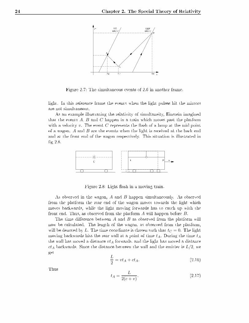
24 Chapter 2. The Spe ial Theory of Relativity

x

tA

BC

leftmirror rightmirror

xBxCxAFigure 2.7: The simultaneous events of 2.6 in another frame.light. In this referen e frame the events when the light pulses hit the mirrorsare not simultaneous.As an example illustrating the relativity of simultaneity, Einstein imaginedthat the events A, B and C happen in a train whi h moves past the platformwith a velo ity v. The event C represents the ash of a lamp at the mid-pointof a wagon. A and B are the events when the light is re eived at the ba k endand at the front end of the wagon respe tively. This situation is illustrated ing 2.8.C A vB

Figure 2.8: Light ash in a moving train.As observed in the wagon, A and B happen simultaneously. As observedfrom the platform the rear end of the wagon moves towards the light whi hmoves ba kwards, while the light moving forwards has to at h up with thefront end. Thus, as observed from the platform A will happen before B.The time dieren e between A and B as observed from the platform willnow be al ulated. The length of the wagon, as observed from the platform,will be denoted by L. The time oordinate is hosen su h that tC = 0. The lightmoving ba kwards hits the rear wall at a point of time tA. During the time tAthe wall has moved a distan e vtA forwards, and the light has moved a distan ectA ba kwards. Sin e the distan e between the wall and the emitter is L/2, weget

L

2= vtA + ctA. (2.16)Thus

tA =L

2(c+ v). (2.17)

2.6 The Lorentz- ontra tion 25In the same manner one ndstB =

L

2(c− v). (2.18)It follows that the time dieren e between A and B as observed from the plat-form is

∆t = tB − tA =γ2vL

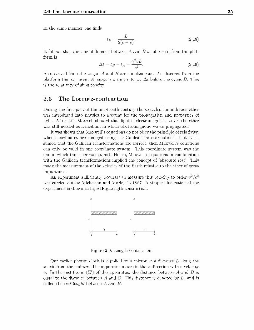
c2. (2.19)As observed from the wagon A and B are simultaneous. As observed from theplatform the rear event A happens a time interval ∆t before the event B. Thisis the relativity of simultaneity.2.6 The Lorentz- ontra tionDuring the rst part of the nineteenth entury the so- alled luminiferous etherwas introdu ed into physi s to a ount for the propagation and properties oflight. After J.C. Maxwell showed that light is ele tromagneti waves the etherwas still needed as a medium in whi h ele tromagneti waves propagated.It was shown that Maxwell's equations do not obey the prin iple of relativity,when oordinates are hanged using the Galilean transformations. If it is as-sumed that the Galilean transformations are orre t, then Maxwell's equations an only be valid in one oordinate system. This oordinate system was theone in whi h the ether was at rest. Hen e, Maxwell's equations in ombinationwith the Galilean transformations implied the on ept of 'absolute rest'. Thismade the measurement of the velo ity of the Earth relative to the ether of greatimportan e.An experiment su iently a urate to measure this velo ity to order v2/c2was arried out by Mi helson and Morley in 1887. A simple illustration of theexperiment is shown in g refFig:Length- ontra tion.

BA L0 BA LFigure 2.9: Length ontra tionOur earlier photon lo k is supplied by a mirror at a distan e L along thex-axis from the emitter. The apparatus moves in the x-dire tion with a velo ityv. In the rest-frame (Σ′) of the apparatus, the distan e between A and B isequal to the distan e between A and C. This distan e is denoted by L0 and is alled the rest length between A and B.

26 Chapter 2. The Spe ial Theory of RelativityLight is emitted from A. Sin e the velo ity of light is isotropi and thedistan es to B and C are equal in Σ′, the light ree ted from B and thatree ted from C have the same travelling time. This was the result of theMi helsonMorley experiment, and it seems that we need no spe ial ee ts su has the Lorentz- ontra tion to explain the experiment.However, before 1905 people believed in the physi al reality of absolute ve-lo ity. The Earth was onsidered to move though an ether with a velo ity that hanged with the seasons. The experiment should therefore be des ribed underthe assumption that the apparatus is moving.Let us therefore des ribe a experiment from our referen e frame Σ, whi hmay be thought of as at rest in the ether. Then a ording to Eq. (2.14) thetravel time of the light being ree ted at C is∆tC = γ

2L0

c. (2.20)For the light moving from A to B we may use Eq. (2.18), and for the light from

B to A Eq. (2.17). This gives∆tB =

L

c− v+

L

c+ v= γ2 2L

c. (2.21)If length is independent of velo ity, then L = L0. In this ase the travellingtimes of the light signals will be dierent. The travelling time dieren e is

∆tB − ∆tC = γ(γ − 1)2L0

c. (2.22)To the lowest order in v/c, γ ≈ 1 + 1

2 (v/c)2, so that∆tB − ∆tC ≈ 1

2

(vc

)2. (2.23)whi h depends upon the velo ity of the apparatus.A ording to the ideas involving an absolute velo ity of the Earth throughthe ether, if one lets the light ree ted at B interfere with the light ree ted at

C (at the position A) then the interferen e pattern should vary with the season.This was not observed. On the ontrary, observations showed that ∆tB = ∆tC .Assuming that length varies with velo ity, Eqs. (2.20) and (2.21), togetherwith this observation, givesL = γ−1L0. (2.24)The result that L < L0 (i.e. the length of a rod is less when it moves than whenit is at rest) is alled the Lorentz- ontra tion.2.7 The Lorentz transformationAn event P has oordinates (t′, x′, 0, 0) in a Cartesian oordinate system asso- iated with a referen e frame Σ′. Thus the distan e from the origin of Σ′ to

2.7 The Lorentz transformation 27P measured with a measuring rod at rest in Σ′ is x′. If the distan e betweenthe origin of Σ′ and the position at the x-axis where P took pla e is measuredwith measuring rods at rest in a referen e frame moving with velo ity v in thex-dire tion relative to Σ′, one nds the length γ−1x due to the Lorentz ontra -tion. Assuming that the origin of Σ and Σ′ oin ided at the point of time t = 0,the origin of Σ′ has an x- oordinate vt at a point of time t. The event P thushas an x- oordinate

x = vt+ γ−1x′ (2.25)orx′ = γ(x− vt). (2.26)The x- oordinate may be expressed in terms of t′ and x′ by letting v → −v,x = γ(x′ + vt′). (2.27)The y and z oordinates are asso iated with axes dire ted perpendi ular to thedire tion of motion. Therefore, they are the same in the two oordinate systems

y = y′ and z = z′. (2.28)Substituting x′ from Eq. (2.26) into Eq. (2.27) reveals the onne tion betweenthe time oordinates of the two oordinate systems,t′ = γ

(t− vx

c2

) (2.29)andt = γ

(t′ +

vx′

c2

). (2.30)The latter term in this equation is nothing but the deviation from simultaneityin Σ for two events that are simultaneous in Σ′.The relations (2.27)(2.30) between the oordinates of Σ and Σ′ represent aspe ial ase of the Lorentz transformations. The above relations are spe ial sin ethe two oordinate systems have the same spatial orientation, and the x and

x′-axes are aligned along the relative velo ity ve tor of the asso iated frames.Su h transformations are alled boosts.For non-relativisti velo ities v ≪ c, the Lorentz transformations (2.27)(2.30) pass over into the orresponding Galilei-transformations.The Lorentz transformation gives a onne tion between the relativity ofsimultaneity and the Lorentz ontra tion. The length of a body is dened as thedieren e between the oordinates of its end points, as measured by simultaneityin the rest-frame of the observer.Consider the wagon of Se tion 2.5. Its rest length is L0 = x′B−x′A. The dif-feren e between the oordinates of the wagon's end-points, xA−xB as measuredin Σ, is given impli itly by the Lorentz transformationx′B − x′A = γ [xB − xA − v(tB − tA)] . (2.31)

28 Chapter 2. The Spe ial Theory of RelativityA ording to the above denition the length (L) of the moving wagon is givenby L = xB − xA with tB = tA.From Eq. (2.31) we then getL0 = γL (2.32)whi h is equivalent to Eq. (2.24).The Lorentz transformation will now be used to dedu e the relativisti for-mulae for velo ity addition. Consider a parti le moving with velo ity u alongthe x′-axis of Σ′. If the parti le was at the origin at t′ = 0, its position at t′ is

x′ = u′t′. Using this relation together with Eqs. (2.27) and (2.28) we nd thevelo ity of the parti le as observed in Σ

u =x

t=

u′ + v

1 + u′vc2

. (2.33)A remarkable property of this expression is that by adding velo ities less thanc one annot obtain a velo ity greater than c. For example, if a parti le moveswith a velo ity c in Σ′ then its velo ity in Σ is also c regardless of Σ's velo ityrelative to Σ′.Equation (2.33) may be written in a geometri al form by introdu ing theso- alled rapidity η dened by

tanh η =u

c(2.34)for a parti le with velo ity u. Similarly the rapidity of Σ′ relative to Σ is

tanh θ =v

c. (2.35)Sin e

tanh(η′ + θ) =tanh η′ + tanh θ

1 + tanh η′ tanh θ, (2.36)the relativisti velo ity addition formula, Eq. (2.33), may be written

η = η′ + θ. (2.37)Sin e rapidities are additive, their introdu tion simplies some al ulations andthey have often been used as variables in elementary parti le physi s.With these new hyperboli variables we an write the Lorentz transformationin a parti ularly simple way. Using Eq. (2.35) in Eqs. (2.27) and (2.30) we ndx = x′ cosh θ + ct′ sinh θ, ct = x′ sinh θ + ct′ cosh θ. (2.38)

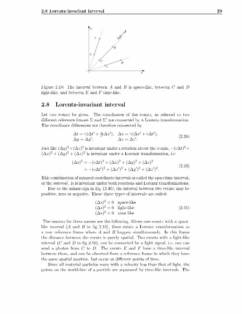
2.8 Lorentz-invariant interval 29

x

tC D light- one

A BE F

Figure 2.10: The interval between A and B is spa e-like, between C and Dlight-like, and between E and F time-like.2.8 Lorentz-invariant intervalLet two events be given. The oordinates of the events, as referred to twodierent referen e frames Σ and Σ′ are onne ted by a Lorentz transformation.The oordinate dieren es are therefore onne ted by∆t = γ(∆t′ + v

c2∆x′), ∆x = γ(∆x′ + v∆t′),

∆y = ∆y′, ∆z = ∆z′.(2.39)Just like (∆y)2+(∆z)2 is invariant under a rotation about the x-axis, −(c∆t)2+

(∆x)2 + (∆y)2 + (∆z)2 is invariant under a Lorentz transformation, i.e.(∆s)2 = −(c∆t)2 + (∆x)2 + (∆y)2 + (∆z)2

= −(c∆t′)2 + (∆x′)2 + (∆y′)2 + (∆z′)2.(2.40)This ombination of squared oordinate-intervals is alled the spa etime interval,or the interval . It is invariant under both rotations and Lorentz transformations.Due to the minus-sign in Eq. (2.40), the interval between two events may bepositive, zero or negative. These three types of intervals are alled:

(∆s)2 > 0 spa e-like(∆s)2 = 0 light-like(∆s)2 < 0 time-like (2.41)The reasons for these names are the following. Given two events with a spa e-like interval (A and B in g 2.10), there exists a Lorentz transformation toa new referen e frame where A and B happen simultaneously. In this framethe distan e between the events is purely spatial. Two events with a light-likeinterval (C and D in g 2.10), an be onne ted by a light signal, i.e. one ansend a photon from C to D. The events E and F have a time-like intervalbetween them, and an be observed from a referen e frame in whi h they havethe same spatial position, but o ur at dierent points of time.Sin e all material parti les move with a velo ity less than that of light, thepoints on the world-line of a parti le are separated by time-like intervals. The

30 Chapter 2. The Spe ial Theory of Relativity urve is then said to be time-like. All time-like urves through a point passinside the light- one from that point.If the velo ity of a parti le is u = ∆x/∆t along the x-axis, Eq. (2.40) gives(∆s)2 = −

(1 − u2

c2

)(c∆t)2. (2.42)In the rest-frame Σ′ of the parti le, ∆x′ = 0, giving

(∆s)2 = −(c∆t′)2. (2.43)The time t′ in the rest-frame of the parti le is the same as the time measuredon a lo k arried by the parti le. It is alled the proper time of the parti le,and denoted by τ . From Eqs. (2.42) and (2.43) it follows that∆τ =

√1 − u2

c2∆t = γ−1∆t (2.44)whi h is an expression of the relativisti time-dilatation.Equation (2.43) is important. It gives the physi al interpretation of a timelike interval between two events. The interval is a measure of the proper timeinterval between the events. This time is measured on a lo k that moves su hthat it is present at both events. In the limit u→ c (the limit of a light signal),

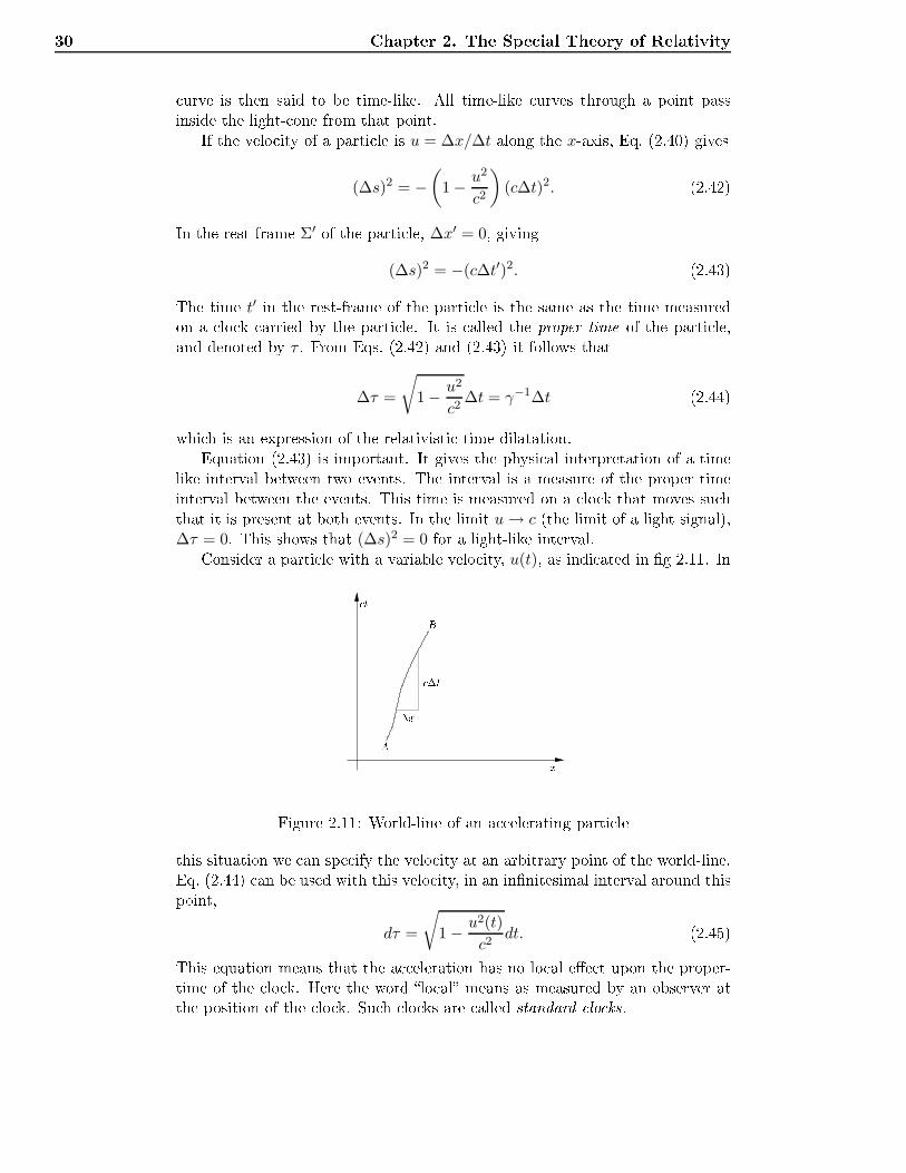
∆τ = 0. This shows that (∆s)2 = 0 for a light-like interval.Consider a parti le with a variable velo ity, u(t), as indi ated in g 2.11. Inx

tx tA

B

Figure 2.11: World-line of an a elerating parti lethis situation we an spe ify the velo ity at an arbitrary point of the world-line.Eq. (2.44) an be used with this velo ity, in an innitesimal interval around thispoint,dτ =

√1 − u2(t)

c2dt. (2.45)This equation means that the a eleration has no lo al ee t upon the proper-time of the lo k. Here the word lo al means as measured by an observer atthe position of the lo k. Su h lo ks are alled standard lo ks.

2.9 The twin-paradox 31If a parti le moves from A to B in g2.11, the proper-time as measured ona standard lo k following the parti le is found by integrating Eq. (2.45)τB − τA =

∫ B

A

√1 − u2(t)

c2dt. (2.46)The relativisti time-dilatation has been veried with great a ura y by obser-vations of unstable elementary parti les with short life-times.An innitesimal spa etime interval

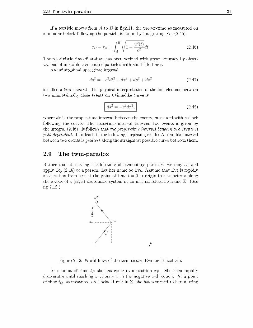
ds2 = −c2dt2 + dx2 + dy2 + dz2 (2.47)is alled a line-element . The physi al interpretation of the line-element betweentwo innitesimally lose events on a time-like urve isds2 = −c2dτ2, (2.48)where dτ is the proper-time interval between the events, measured with a lo kfollowing the urve. The spa etime interval between two events is given bythe integral (2.46). It follows that the proper-time interval between two events ispath dependent. This leads to the following surprising result: A time-like intervalbetween two events is greatest along the straightest possible urve between them.2.9 The twin-paradoxRather than dis ussing the life-time of elementary parti les, we may as wellapply Eq. (2.46) to a person. Let her name be Eva. Assume that Eva is rapidlya eleration from rest at the point of time t = 0 at origin to a velo ity v alongthe x-axis of a (ct, x) oordinate system in an inertial referen e frame Σ. (Seeg 2.12.)

xP

tQEva tP Elizabeth

Figure 2.12: World-lines of the twin sisters Eva and Elizabeth.At a point of time tP she has ome to a position xP . She then rapidlyde elerates until rea hing a velo ity v in the negative x-dire tion. At a pointof time tQ, as measured on lo ks at rest in Σ, she has returned to her starting

32 Chapter 2. The Spe ial Theory of Relativitylo ation. If we negle t the brief periods of a eleration, Eva's travelling time asmeasured on a lo k whi h she arries with her istEva =

(1 − v2

c2

)1/2

tQ. (2.49)Now assume that Eva has a twin-sister named Elizabeth who remains at rest atthe origin of Σ.Elizabeth has be ome older by τElizabeth = tQ during Eva's travel, so thatτEva =

(1 − v2

c2

)1/2

τElizabeth. (2.50)For example, if Eva travelled to Alpha Centauri (the Sun's nearest neighbourat four light years) with a velo ity v = 0.8c, she is would be gone for tenyears as measured by Elizabeth. Therefore Elizabeth has aged 10 years duringEva's travel. A ording to Eq. (2.50), Eva has only aged 6 years. A ording toElizabeth, Eva has aged less than herself during her travels.The prin iple of relativity, however, tells that Eva an onsider herself as atrest and Elizabeth as the traveller. A ording to Eva it is Elizabeth who hasonly aged by 6 years, while Eva has aged by 10 years during the time they areapart.What happens? How an the twin-sisters arrive at the same predi tion asto how mu h ea h of them age during the travel? In order to arrive at a learanswer to these questions, we shall have to use a result from the general theoryof relativity. The twin-paradox will be taken up again in Chapter 5.2.10 Hyperboli motionWith referen e to an inertial referen e frame it is easy to des ribe relativisti a elerated motion. The spe ial theory of relativity is in no way limited todes ribe motion with onstant velo ity.Let a parti le move with a variable velo ity u(t) = dx/dt along the x-axisin Σ. The frame Σ′ moves with velo ity v in the same dire tion relative toΣ. In this frame the parti le-velo ity is u′(t′) = dx′/dt′. At every moment thevelo ities u and u′ are onne ted by the relativisti formula for velo ity addition,Eq. (2.33). Thus, a velo ity hange du′ in Σ′ and the orresponding velo ity hange du in Σ are related using Eq. (2.30) by

dt =dt′ + v

c2dx′

√1 − v2

c2

=1 + u′v

c2√1 − v2

c2

dt′. (2.51)Combining these expressions we obtain the relationship between the a elerationof the parti le as measured in Σ and in Σ′

a =du

dt=

(1 − v2

c2

)3/2

(1 + u′v

c2

)3 a′. (2.52)

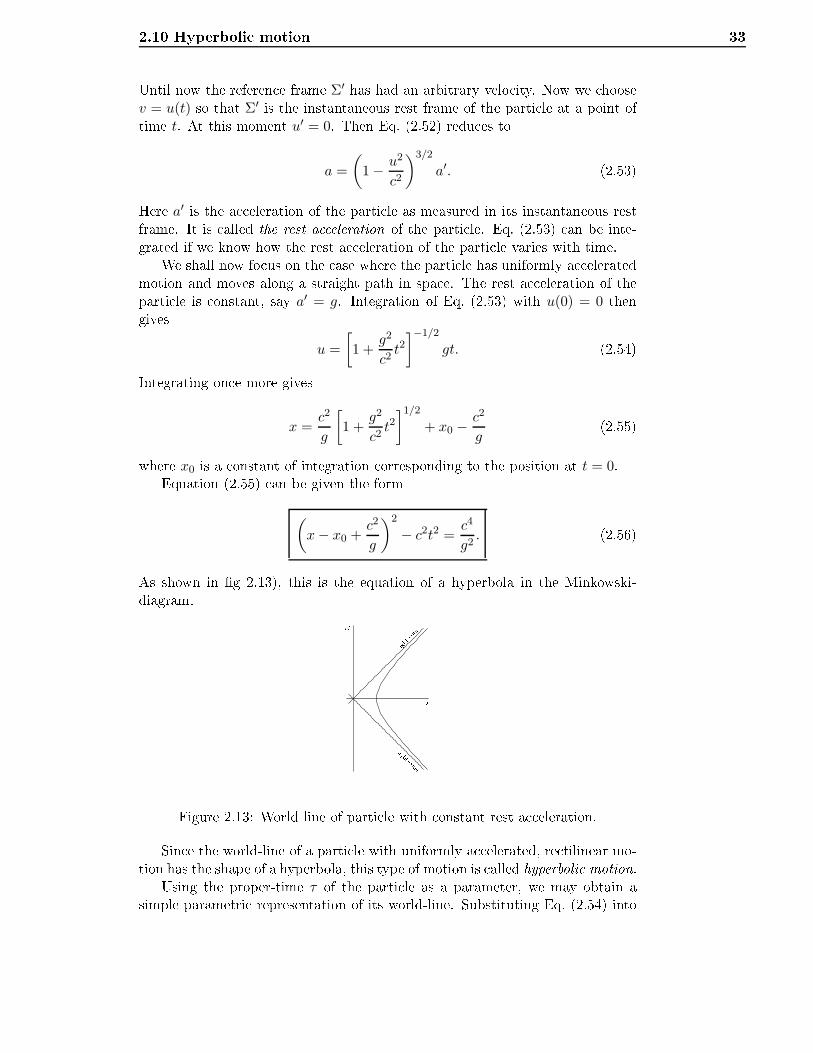
2.10 Hyperboli motion 33Until now the referen e frame Σ′ has had an arbitrary velo ity. Now we hoosev = u(t) so that Σ′ is the instantaneous rest frame of the parti le at a point oftime t. At this moment u′ = 0. Then Eq. (2.52) redu es to

a =

(1 − u2

c2

)3/2

a′. (2.53)Here a′ is the a eleration of the parti le as measured in its instantaneous restframe. It is alled the rest a eleration of the parti le. Eq. (2.53) an be inte-grated if we know how the rest a eleration of the parti le varies with time.We shall now fo us on the ase where the parti le has uniformly a eleratedmotion and moves along a straight path in spa e. The rest a eleration of theparti le is onstant, say a′ = g. Integration of Eq. (2.53) with u(0) = 0 thengivesu =

[1 +

g2

c2t2]−1/2

gt. (2.54)Integrating on e more givesx =

c2

g

[1 +

g2

c2t2]1/2

+ x0 −c2

g(2.55)where x0 is a onstant of integration orresponding to the position at t = 0.Equation (2.55) an be given the form

(x− x0 +

c2

g

)2

− c2t2 =c4

g2. (2.56)As shown in g 2.13), this is the equation of a hyperbola in the Minkowski-diagram.

light- one

light- onex

t

Figure 2.13: World line of parti le with onstant rest a eleration.Sin e the world-line of a parti le with uniformly a elerated, re tilinear mo-tion has the shape of a hyperbola, this type of motion is alled hyperboli motion.Using the proper-time τ of the parti le as a parameter, we may obtain asimple parametri representation of its world-line. Substituting Eq. (2.54) into

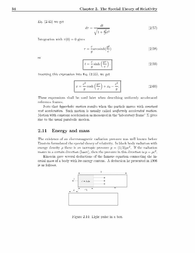
34 Chapter 2. The Spe ial Theory of RelativityEq. (2.45) we getdτ =

dt√1 + g2

c2t2

(2.57)Integration with τ(0) = 0 givesτ =

c

garcsinh(

gt

c) (2.58)or

t =c

gsinh

(gτc

). (2.59)Inserting this expression into Eq. (2.55), we get

x =c2

gcosh

(gτc

)+ x0 −

c2

g. (2.60)These expressions shall be used later when des ribing uniformly a eleratedreferen e frames.Note that hyperboli motion results when the parti le moves with onstantrest a eleration. Su h motion is usually alled uniformly a elerated motion.Motion with onstant a eleration as measured in the laboratory frame Σ givesrise to the usual paraboli motion.2.11 Energy and massThe existen e of an ele tromagneti radiation pressure was well known beforeEinstein formulated the spe ial theory of relativity. In bla k body radiation withenergy density ρ there is an isotropi pressure p = (1/3)ρc2. If the radiationmoves in a ertain dire tion (laser), then the pressure in this dire tion is p = ρc2.Einstein gave several dedu tions of the famous equation onne ting the in-ertial mass of a body with its energy ontent. A dedu tion he presented in 1906is as follows.

x MLv tV = A t

Figure 2.14: Light pulse in a box.

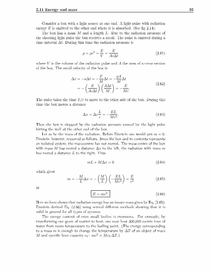
2.11 Energy and mass 35Consider a box with a light sour e at one end. A light pulse with radiationenergy E is emitted to the other end where it is absorbed. (See g 2.14).The box has a mass M and a length L. Due to the radiation pressure ofthe shooting light pulse the box re eives a re oil. The pulse is emitted during atime interval ∆t. During this time the radiation pressure isp = ρc2 =

E

V=

E

Ac∆t(2.61)where V is the volume of the radiation pulse and A the area of a ross-se tionof the box. The re oil velo ity of the box is

∆v = −a∆t = − F

M∆t = −pA

M∆t

= −(

E

Ac∆t

)(A∆t

M

)= − E

Mc.

(2.62)The pulse takes the time L/c to move to the other side of the box. During thistime the box moves a distan e∆x = ∆v

L

c= − EL

Mc2. (2.63)Then the box is stopped by the radiation pressure aused by the light pulsehitting the wall at the other end of the box.Let m be the mass of the radiation. Before Einstein one would put m = 0.Einstein, however, reasoned as follows. Sin e the box and its ontents representsan isolated system, the mass- entre has not moved. The mass entre of the boxwith mass M has moved a distan e ∆x to the left, the radiation with mass mhas moved a distan e L to the right. Thus

mL+M∆x = 0 (2.64)whi h givesm = −M

L∆x = −

(M

L

)(− EL

Mc2

)=E

c2(2.65)or

E = mc2. (2.66)Here we have shown that radiation energy has an innate mass given by Eq. (2.65).Einstein derived Eq. (2.66) using several dierent methods showing that it isvalid in general for all types of systems.The energy ontent of even small bodies is enormous. For example, bytransforming one gram of matter to heat, one may heat 300,000 metri tons ofwater from room temperature to the boiling point. (The energy orrespondingto a mass m is enough to hange the temperature by ∆T of an obje t of massM and spe i heat apa ity cV : mc2 = McV ∆T .)

36 Chapter 2. The Spe ial Theory of Relativity2.12 Relativisti in rease of massIn the spe ial theory of relativity, for e is dened as rate of hange of momentum.We onsider a body that gets a hange of energy dE due to the work performedon it by a for e F . A ording to Eq. (2.66) and the denition of work (for etimes distan e) the body gets a hange of mass dm, given byc2dm = dE = Fds = Fvdt = vd(mv) = mvdv + v2dm, (2.67)whi h gives ∫ m

m0

dm

m=

∫ v

0

vdv

c2 − v2, (2.68)where m0 is the rest mass of the body i.e. its mass as measured by anobserver omoving with the body and m its mass when its velo ity is equal to

v. Integration givesm =

m0√1 − v2

c2

= γm0. (2.69)In the ase of small velo ities ompared to the velo ity of light we may use theapproximation √1 − v2

c2≈ 1 +

1

2

v2

c2. (2.70)With this approximation Eqs. (2.66) and (2.69) give

E ≈ m0c2 +

1

2m0v

2. (2.71)This equation shows that the total energy of a body en ompasses its rest-energym0 and its kineti energy. In the non-relativisti limit the kineti energy ism0v

2/2. The relativisti expression for the kineti energy isEK = E −m0c

2 = (γ − 1)m0c2. (2.72)Note that EK → ∞ when v → c.A ording to Eq. (2.33), it is not possible to obtain a velo ity greater thanthat of light by adding velo ities. Equation (2.72) gives a dynami al reason thatmaterial parti les annot be a elerated up to and above the velo ity of light.2.13 Ta hyonsParti les annot pass the velo ity-barrier represented by the velo ity of light.However, the spe ial theory of relativity permits the existen e of parti les thathave always moved with a velo ity v > c. Su h parti les are alled ta hyons.Ta hyons have spe ial properties that have been used in the experimentalsear hes for them. There is urrently no observational eviden e for the physi alexisten e of ta hyons.

2.13 Ta hyons 37There are also ertain theoreti al di ulties with the existen e of ta hyons.The spe ial theory of relativity, applied to ta hyons leads to the following para-dox. Using a ta hyon telephone a person, A, emits a ta hyon to B at a pointof time t1. B moves away from A. The ta hyon is ree ted by B and rea hA before it was emitted, see g 2.15. If the ta hyon ould arry information itmight bring an order to destroy the ta hyon emitter when it arrives ba k at A.

t1t2

t′R

ct ct′

Simultaneity of Ax

x′

Simultaneity

of B

Figure 2.15: A emits a ta hyon at the point of time t1. It is ree ted by B andarrives at A at a point of time t2 before t1. Note that the arrival event at A islater than the ree tion event as measured by B.To avoid similar problems in regards to the energy-ex hange between ta hyonsand ordinary matter, a reinterpretation prin iple is introdu ed for ta hyons. For ertain observers a ta hyon will move ba kwards in time, i.e. the observer ndsthat the ta hyon is re eived before it was emitted. Spe ial relativity tells usthat su h a ta hyon is always observed to have negative energy.A ording to the reinterpretation prin iple, the observer will interpret hisobservations to mean that a ta hyon with positive energy moves forward intime. In this way, one nds that the energy-ex hange between ta hyons andordinary matter pro eeds in a ordan e with the prin iple of ausality.However, the reinterpretation prin iple annot be used to remove the prob-lems asso iated with ex hange of information between ta hyons and ordinarymatter. The ta hyon telephone paradox annot be resolved by means of thereinterpretation prin iple. The on lusion is that if ta hyons exist, they annotbe arriers of information in our slowly-moving world.

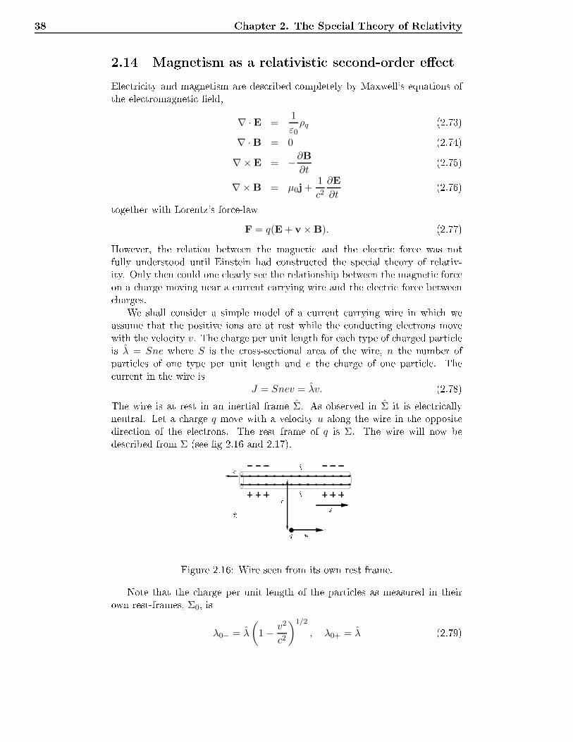
38 Chapter 2. The Spe ial Theory of Relativity2.14 Magnetism as a relativisti se ond-order ee tEle tri ity and magnetism are des ribed ompletely by Maxwell's equations ofthe ele tromagneti eld,∇ · E =

1

ε0ρq (2.73)

∇ · B = 0 (2.74)∇× E = −∂B

∂t(2.75)

∇× B = µ0j +1

c2∂E

∂t(2.76)together with Lorentz's for e-law

F = q(E + v × B). (2.77)However, the relation between the magneti and the ele tri for e was notfully understood until Einstein had onstru ted the spe ial theory of relativ-ity. Only then ould one learly see the relationship between the magneti for eon a harge moving near a urrent arrying wire and the ele tri for e between harges.We shall onsider a simple model of a urrent arrying wire in whi h weassume that the positive ions are at rest while the ondu ting ele trons movewith the velo ity v. The harge per unit length for ea h type of harged parti leis λ = Sne where S is the ross-se tional area of the wire, n the number ofparti les of one type per unit length and e the harge of one parti le. The urrent in the wire isJ = Snev = λv. (2.78)The wire is at rest in an inertial frame Σ. As observed in Σ it is ele tri allyneutral. Let a harge q move with a velo ity u along the wire in the oppositedire tion of the ele trons. The rest frame of q is Σ. The wire will now bedes ribed from Σ (see g 2.16 and 2.17).

r q+u

v J

Figure 2.16: Wire seen from its own rest frame.Note that the harge per unit length of the parti les as measured in theirown rest-frames, Σ0, isλ0− = λ

(1 − v2

c2

)1/2

, λ0+ = λ (2.79)

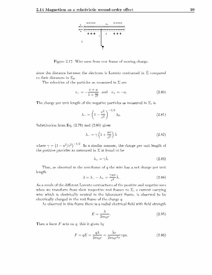
2.14 Magnetism as a relativisti se ond-order ee t 39r q

+uvFigure 2.17: Wire seen from rest frame of moving harge.sin e the distan e between the ele trons is Lorentz ontra ted in Σ omparedto their distan es in Σ0.The velo ities of the parti les as measured in Σ arev− = − v + u

1 + uvc2

and v+ = −u. (2.80)The harge per unit length of the negative parti les as measured in Σ, isλ− =

(1 − v2

−c2

)−1/2

λ0. (2.81)Substitution from Eq. (2.79) and (2.80) givesλ− = γ

(1 +

uv

c2

)λ (2.82)where γ =

(1 − u2/c2

)−1/2. In a similar manner, the harge per unit length ofthe positive parti les as measured in Σ is found to beλ+ = γλ. (2.83)Thus, as observed in the rest-frame of q the wire has a net harge per unitlength

λ = λ− − λ+ =γuv

c2λ. (2.84)As a result of the dierent Lorentz ontra tions of the positive and negative ionswhen we transform from their respe tive rest frames to Σ, a urrent arryingwire whi h is ele tri ally neutral in the laboratory frame, is observed to beele tri ally harged in the rest frame of the harge q.As observed in this frame there is a radial ele tri al eld with eld strength

E =λ

2πǫ0r. (2.85)Then a for e F a ts on q, this is given by

F = qE =qλ

2πǫ0r=

λv

2πǫ0c2rγqu. (2.86)

40 Chapter 2. The Spe ial Theory of RelativityIf a for e a ts upon q as observed in Σ then a for e also a ts on q as observedin Σ. A ording to the relativisti transformation of a for e omponent in thesame dire tion as the relative velo ity between Σ and Σ, this for e isF = γ−1F =

λv

2πǫ0c2rqu. (2.87)Inserting J = λv from Eq. (2.78) and using c2 = (ǫ0µ0)

−1 (where µ0 is thepermeability of a va uum) we obtainF =

µ0J

2πrqu. (2.88)This is exa tly the expression obtained if we al ulate the magneti ux-density

B around the urrent arrying wire using Ampere's ir uit lawB = µ0

J

2πr(2.89)and use the for e-law (Eq. (2.77)) for a harge moving in a magneti eld

F = quB. (2.90)We have seen here how a magneti for e appears as a result of an ele trostati for e and the spe ial theory of relativity. The onsiderations above have alsodemonstrated that a for e whi h is identied as ele trostati in one frame ofreferen e is observed as a magneti for e in another frame. In other words, theele tri and the magneti for e are really the same. What an observer names itdepends upon his state of motion.

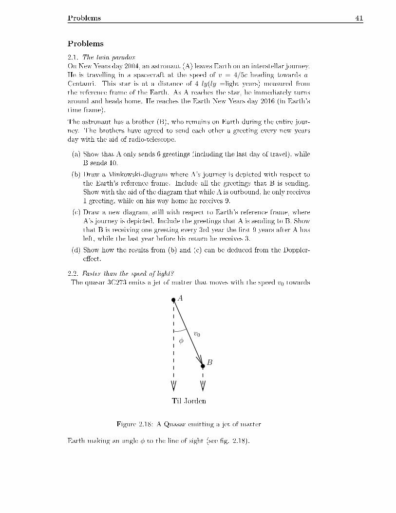
Problems 41Problems2.1. The twin-paradoxOn New Years day 2004, an astronaut (A) leaves Earth on an interstellar journey.He is travelling in a spa e raft at the speed of v = 4/5c heading towards a-Centauri. This star is at a distan e of 4 ly(ly =light years) measured fromthe referen e frame of the Earth. As A rea hes the star, he immediately turnsaround and heads home. He rea hes the Earth New Years day 2016 (in Earth'stime frame).The astronaut has a brother (B), who remains on Earth during the entire jour-ney. The brothers have agreed to send ea h other a greeting every new yearsday with the aid of radio-teles ope.(a) Show that A only sends 6 greetings (in luding the last day of travel), whileB sends 10.(b) Draw a Minkowski-diagram where A's journey is depi ted with respe t tothe Earth's referen e frame. In lude all the greetings that B is sending.Show with the aid of the diagram that while A is outbound, he only re eives1 greeting, while on his way home he re eives 9.( ) Draw a new diagram, still with respe t to Earth's referen e frame, whereA's journey is depi ted. In lude the greetings that A is sending to B. Showthat B is re eiving one greeting every 3rd year the rst 9 years after A hasleft, while the last year before his return he re eives 3.(d) Show how the results from (b) and ( ) an be dedu ed from the Doppler-ee t.2.2. Faster than the speed of light?The quasar 3C273 emits a jet of matter that moves with the speed v0 towards

Til Jorden

A

φ

B

v0

Figure 2.18: A Quasar emitting a jet of matterEarth making an angle φ to the line of sight (see g. 2.18).

42 Chapter 2. The Spe ial Theory of Relativity(a) Assume that two signals are sent towards the Earth simultaneously, onefrom A and one from B. How mu h earlier will the signal from B rea h theEarth ompared to that from A?(b) Find an expression of the transverse distan e that the emitted part hasmoved when it rea hes B. How mu h time (relative to the Earth) has thispart been travelling?( ) Let v be the transverse velo ity and relate it to v0. The observed (thetransverse) speed of the light-sour e is v = 10c. Find v0 when we assumethat φ = 10. What is the largest possible φ?2.3. Two su essive boosts in dierent dire tionsLet us onsider Lorentz transformations without rotation (boosts). A boostin the x-dire tion is given byx = g(x′ + bct′), y = y′, z = z′ t = g(t′ + bx′/c)

γ = 1√1−b2 b = v

c (2.91)This an be written asxµ = Λµµ′x

µ′ (2.92)where Λµµ′ is the matrixΛµµ′ =

g gb 0 0gb g 0 00 0 1 00 0 0 1

(2.93)(a) Show that (2.92) and (2.93) yield (2.91). Find the transformation matrix,Λµµ′ , for a boost in the negative y-dire tion.(b) Two su essive Lorentz transformations are given by the matrix produ tof ea h matrix. Find ΛµaΛaµ′ and Λµa Λaµ′ . Are the produ t of two boosts aboost? The matrix for a general boost in arbitrary dire tion is given by

Λ00 = g,

Λ0m = Λm0 = gbm,

Λmm′ = δmm′ +bmbm′

b2(g − 1),

g =1√

1 − b2, b2 = bmbm, m,m′ = 1, 2, 3 (2.94)Does the set of all possible boosts form a group?2.4. Length- ontra tion and time-dilatation(a) A rod with length ℓ is moving with onstant velo ity v with respe t to theinertial frame Σ. The length of the rod is parallel to v, whi h we will forsimpli ity's sake assume is parallel to the x-axis. At time t = 0, the rearend of the rod is in the origin of Σ. What do we mean by the length of

Problems 43su h a moving rod? Des ribe how an observer an nd this length. Drawthe rod in a Minkowski diagram and explain how the length of the rod anbe read of the diagram. Using the Lorentz transformations, al ulate theposition of the endpoints of the rod as a fun tion of time t. Show that thelength of the rod, as measured in Σ, is shorter than its rest length ℓ.(b) The rod has the same velo ity as before, but now the rod makes an anglewith v. In an inertial frame whi h follows the movement of the rod (Σ′),this angle is a′ = 45 (with the x-axis in Σ). What is the angle betweenthe velo ity v and the rod when measured in Σ? What is the length of therod as a fun tion of a′, as measured from Σ?( ) We again assume that a′ = 0. At the entre of the rod there is a ashthat sends light signals with a time interval τ0 between every ash. In theframe Σ′, the light signals will rea h the two ends simultaneously. Showthat these two events are not simultaneous in Σ. Find the time dieren ebetween these two events.Show that the time interval τ measured from Σ between ea h ash, is largerthan the interval τ0 measured in Σ′.An observer in Σ is lo ated at the origin. He measures the time-interval∆t between every time he re eives a light signal. Find ∆t in terms of thespeed v, and he k whether ∆t is greater or less than τ .(d) The length of the rod is now onsidered to be ell = 1m and its speed, asmeasured in Σ, is v = 3

5c. As before, we assume that the rod is movingparallel to the x-axis, but this time at a distan e of y = 10m from theaxis. A measuring ribbon is stret hed out along the traje tory of therod. This ribbon is at rest in Σ. An observer at the origin sees the rodmove along the ba kground ribbon. The ribbon has ti k-marks along itwhi h orrespond to the x oordinates. The rods length an be measuredby taking a photograph of the rod and the ribbon. Is the length that isdire tly measured from the photograph identi al to the length of the rodin Σ?In one of the photographs the rod is symmetri ally entered with respe t tox = 0. What is the length of the rod as measured using this photograph?Another photograph shows the rod with its trailing edge at x = 10m.At what point will the leading edge of the rod be on this photograph?Compare with the length of the rod in the Σ frame.(e) At one point along the traje tory the rod passes through a box whi h isopen at both ends and stationary in Σ. This box is shorter than the restlength of the rod, but longer that the length of the rod as measured in Σ.At a ertain time in Σ, the entire rod is therefore inside the box. At thistime the box is losed at both ends, trapping the rod inside. The rod is alsobrought to rest. It is assumed that the box is strong enough to withstandthe impa t with the rod.What happens to the rod? Des ribe what happens as observed from Σ andΣ′. Draw a Minkowski diagram. This is an example of why the theory ofrelativity has di ulty with the on ept of absolute rigid bodies. What is

44 Chapter 2. The Spe ial Theory of Relativitythe reason for this di ulty?2.5. Ree tion angles o moving mirrors(a) The ree tion angle of light equals the in iden e angle of the light. Showthat this is also the ase for mirrors that are moving parallel to the ree tionsurfa e.(b) A mirror is moving with a speed v in a dire tion orthogonal to the ree tionsurfa e. Light is sent towards the mirror with an angle φ. Find the angleof the ree ted light as a fun tion of v and φ. What is the frequen y tothe ree ted light expressed in terms of its original frequen y f?2.6. Minkowski-diagramThe referen e frame Σ′ is moving relative to the frame Σ at a speed of v = 0.6c.The movement is parallel to the x-axes of the two frames.Draw the x′ and the ct′-axis in the Minkowski-diagram of Σ. Points separated by1m are marked along both axes. Draw these points in the Minkowski-diagramas for both frames.Show where the lines of simultaneity for Σ′ are in the diagram. Also show wherethe x′ = constant line is.Assume that the frames are equipped with measuring rods and lo ks that areat rest in their respe tive frames. How an we use the Minkowski-diagram tomeasure the length- ontra tion of the rod that is in rest at Σ′? Similarly, how an we measure the length- ontra tion of the rod in Σ when measured from Σ?Show how the time-dilatation of the lo ks an be measured from the diagram.2.7. Robb's Lorentz invariant spa etime interval formula (A.A. Robb, 1936)Show that the spa etime interval between the origin event and the ree tionevent in g. 2.2 is s = c

√tAtB .2.8. The Doppler ee tA radar antenna emits radio pulses with a wavelength of λ = 1.0cm, at a time-interval τ = 1.0s. An approa hing spa e raft is being registered by the radar.Draw a Minkowski-diagram for the referen e frame Σ. The antenna is at rest inthis frame. In this diagram, indi ate the position of1.the antenna,2.the spa e raft, and3.the outgoing and ree ted radar pulses.Cal ulate the time dieren e ∆t1 between two subsequent pulses as measuredin the spa e raft. What is the wavelength of these signals?Cal ulate the time dieren e ∆t2 between two ree ted signals, as it is measuredfrom the antenna's re eiver? At what wavelength will these signals be?

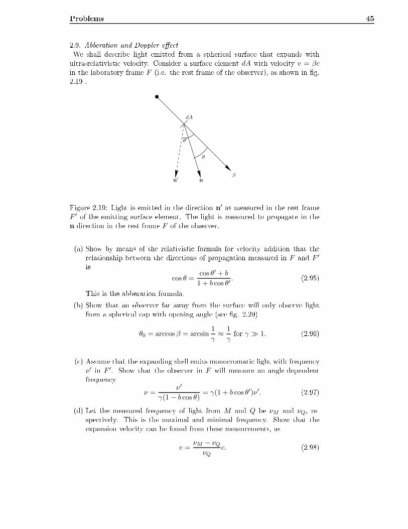
Problems 452.9. Abberation and Doppler ee tWe shall des ribe light emitted from a spheri al surfa e that expands withultra-relativisti velo ity. Consider a surfa e element dA with velo ity v = βcin the laboratory frame F (i.e. the rest frame of the observer), as shown in g.2.19 .n

dA

n′

β

θ′

θ

Figure 2.19: Light is emitted in the dire tion n′ as measured in the rest frameF ′ of the emitting surfa e element. The light is measured to propagate in then-dire tion in the rest frame F of the observer.(a) Show by means of the relativisti formula for velo ity addition that therelationship between the dire tions of propagation measured in F and F ′is

cos θ =cos θ′ + b

1 + b cos θ′. (2.95)This is the abberation formula.(b) Show that an observer far away from the surfa e will only observe lightfrom a spheri al ap with opening angle (see g. 2.20)

θ0 = arccos β = arcsin1

γ≈ 1

γfor γ ≫ 1. (2.96)( ) Assume that the expanding shell emits mono romati light with frequen y

ν ′ in F ′. Show that the observer in F will measure an angle-dependentfrequen yν =

ν ′

γ(1 − b cos θ)= γ(1 + b cos θ′)ν ′. (2.97)(d) Let the measured frequen y of light from M and Q be νM and νQ, re-spe tively. This is the maximal and minimal frequen y. Show that theexpansion velo ity an be found from these measurements, as

v =νM − νQνQ

c. (2.98)

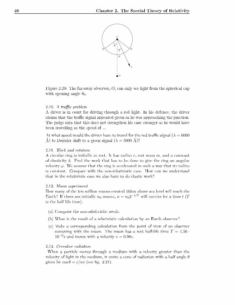
46 Chapter 2. The Spe ial Theory of RelativityM

O

C

QQ

β

θ0

θ

Figure 2.20: The far-away observer, O, an only see light from the spheri al apwith opening angle θ0.2.10. A tra problemA driver is in ourt for driving through a red light. In his defen e, the driver laims that the tra signal appeared green as he was approa hing the jun tion.The judge says that this does not strengthen his ase stronger as he would havebeen travelling at the speed of ...At what speed would the driver have to travel for the red tra signal (λ = 6000Å) to Doppler shift to a green signal (λ = 5000 Å)?2.11. Work and rotationA ir ular ring is initially at rest. It has radius r, rest mass m, and a onstantof elasti ity k. Find the work that has to be done to give the ring an angularvelo ity ω. We assume that the ring is a elerated in su h a way that its radiusis onstant. Compare with the non-relativisti ase. How an we understandthat in the relativisti ase we also have to do elasti work?2.12. Muon experimentHow many of the ten million muons reated 10km above sea level will rea h theEarth? If there are initially n0 muons, n = n02−t/T will survive for a time t (Tis the half-life time).(a) Compute the non-relativisti result.(b) What is the result of a relativisti al ulation by an Earth observer?( ) Make a orresponding al ulation from the point of view of an observer omoving with the muon. The muon has a rest half-life time T = 1.56 ·

10−6s and moves with a velo ity v = 0.98c.2.13. Cerenkov radiationWhen a parti le moves through a medium with a velo ity greater than thevelo ity of light in the medium, it emits a one of radiation with a half angle θgiven by cos θ = c/nv (see g. 2.21).

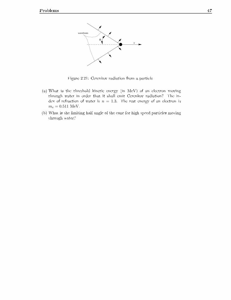
Problems 47wavefronts

θv

Figure 2.21: Cerenkov radiation from a parti le(a) What is the threshold kineti energy (in MeV) of an ele tron movingthrough water in order that it shall emit Cerenkov radiation? The in-dex of refra tion of water is n = 1.3. The rest energy of an ele tron isme = 0.511 MeV.(b) What is the limiting half angle of the one for high speed parti les movingthrough water?

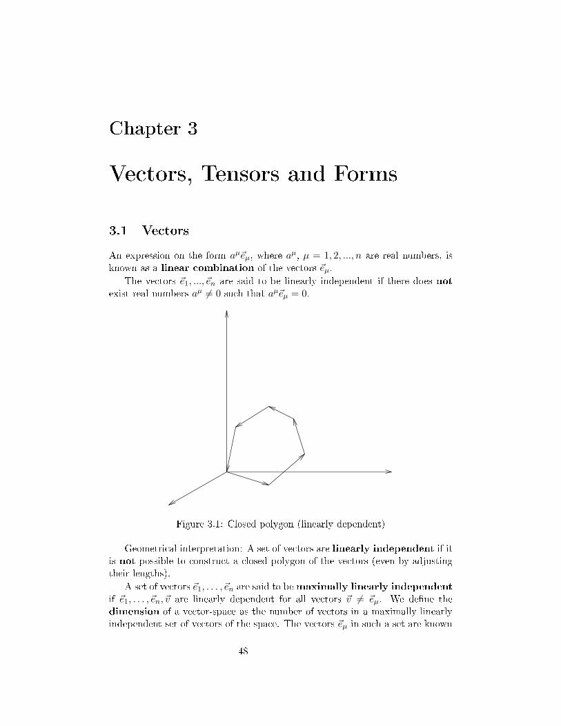
Chapter 3Ve tors, Tensors and Forms3.1 Ve torsAn expression on the form aµ~eµ, where aµ, µ = 1, 2, ..., n are real numbers, isknown as a linear ombination of the ve tors ~eµ.The ve tors ~e1, ..., ~en are said to be linearly independent if there does notexist real numbers aµ 6= 0 su h that aµ~eµ = 0.

Figure 3.1: Closed polygon (linearly dependent)Geometri al interpretation: A set of ve tors are linearly independent if itis not possible to onstru t a losed polygon of the ve tors (even by adjustingtheir lengths).A set of ve tors ~e1, . . . , ~en are said to bemaximally linearly independentif ~e1, . . . , ~en, ~v are linearly dependent for all ve tors ~v 6= ~eµ. We dene thedimension of a ve tor-spa e as the number of ve tors in a maximally linearlyindependent set of ve tors of the spa e. The ve tors ~eµ in su h a set are known48

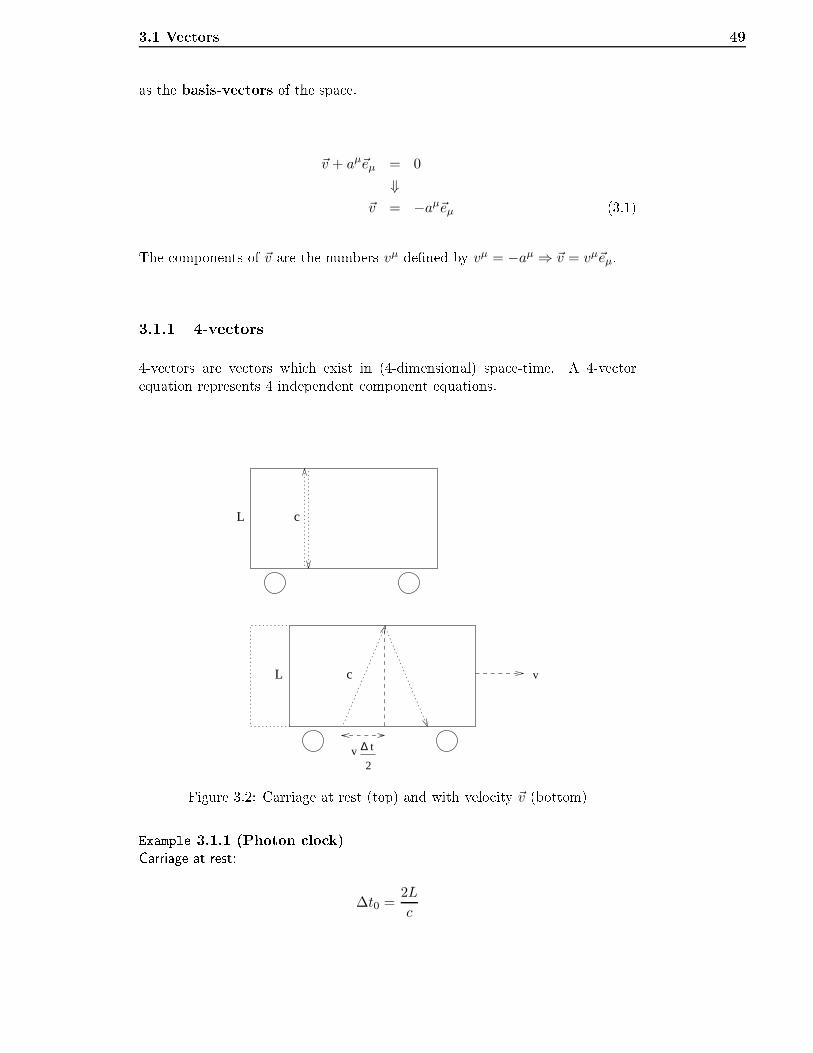
3.1 Ve tors 49as the basis-ve tors of the spa e.~v + aµ~eµ = 0

⇓~v = −aµ~eµ (3.1)The omponents of ~v are the numbers vµ dened by vµ = −aµ ⇒ ~v = vµ~eµ.3.1.1 4-ve tors4-ve tors are ve tors whi h exist in (4-dimensional) spa e-time. A 4-ve torequation represents 4 independent omponent equations.

L c

cL

v ∆ t

2

v

Figure 3.2: Carriage at rest (top) and with velo ity ~v (bottom)Example 3.1.1 (Photon lo k)Carriage at rest:∆t0 =

2L

c

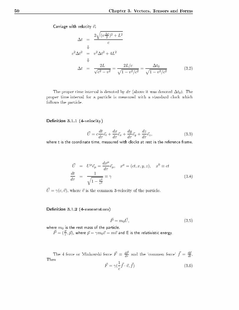
50 Chapter 3. Ve tors, Tensors and FormsCarriage with velo ity ~v:∆t =

2√

(v∆t2 )2 + L2

c⇓

c2∆t2 = v2∆t2 + 4L2

⇓

∆t =2L√c2 − v2

=2L/c√

1 − v2/c2=

∆t0√1 − v2/c2

(3.2)The proper time-interval is denoted by dτ (above it was denoted ∆t0). Theproper time-interval for a parti le is measured with a standard lo k whi hfollows the parti le.Denition 3.1.1 (4-velo ity)~U = c

dt

dτ~et +

dx

dτ~ex +

dy

dτ~ey +

dz

dτ~ez, (3.3)where t is the oordinate time, measured with lo ks at rest in the referen e frame.

~U = Uµ~eµ =dxµ

dτ~eµ, xµ = (ct, x, y, z), x0 ≡ ct

dt

dτ=

1√1 − v2

c2

≡ γ (3.4)~U = γ(c, ~v), where ~v is the ommon 3-velo ity of the parti le.Denition 3.1.2 (4-momentum)

~P = m0~U, (3.5)where m0 is the rest mass of the parti le.

~P = (Ec , ~p), where ~p = γm0~v = m~v and E is the relativisti energy.The 4-for e or Minkowski-for e ~F ≡ d~Pdτ and the ' ommon for e' ~f = d~p

dt .Then~F = γ(

1

c~f · ~v, ~f) (3.6)

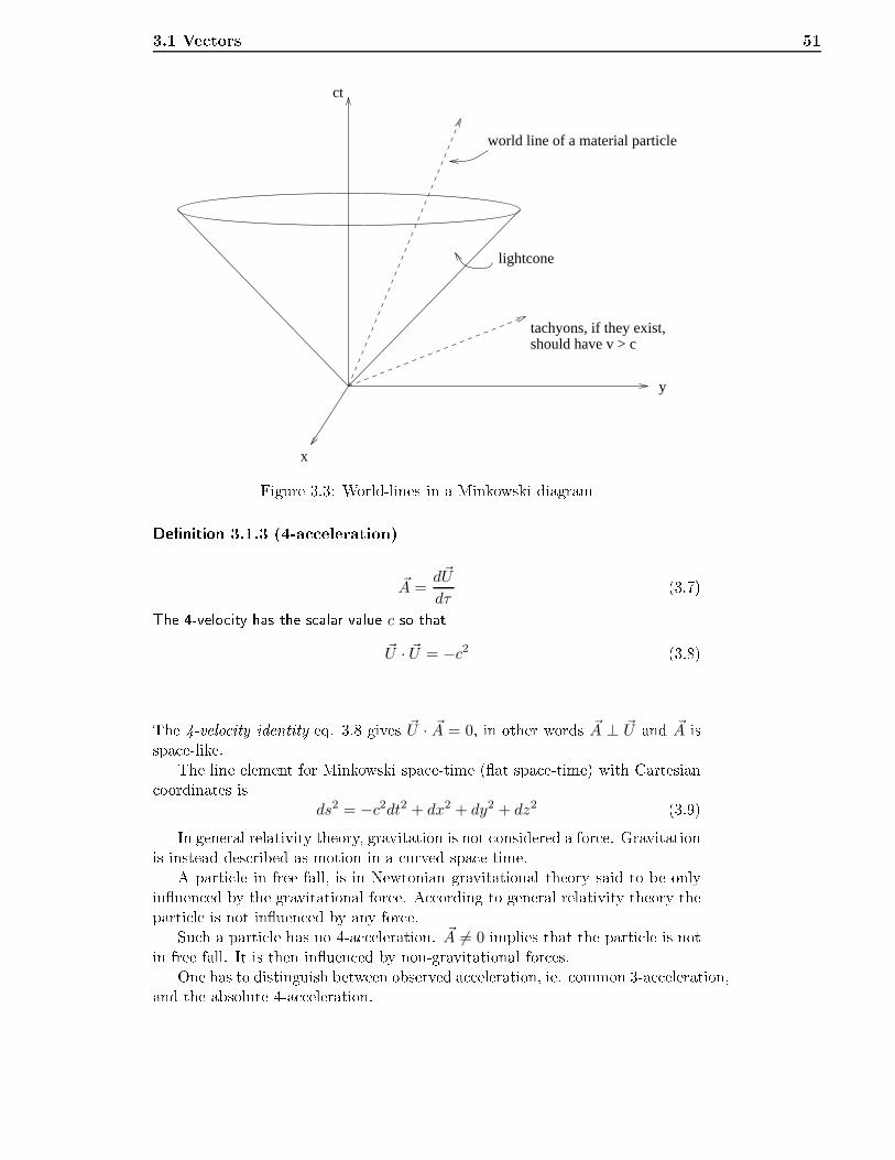
3.1 Ve tors 51lightcone

world line of a material particle

ct

y

x

should have v > ctachyons, if they exist,

Figure 3.3: World-lines in a Minkowski diagramDenition 3.1.3 (4-a eleration)~A =

d~U

dτ(3.7)The 4-velo ity has the s alar value c so that

~U · ~U = −c2 (3.8)The 4-velo ity identity eq. 3.8 gives ~U · ~A = 0, in other words ~A ⊥ ~U and ~A isspa e-like.The line element for Minkowski spa e-time (at spa e-time) with Cartesian oordinates isds2 = −c2dt2 + dx2 + dy2 + dz2 (3.9)In general relativity theory, gravitation is not onsidered a for e. Gravitationis instead des ribed as motion in a urved spa e-time.A parti le in free fall, is in Newtonian gravitational theory said to be onlyinuen ed by the gravitational for e. A ording to general relativity theory theparti le is not inuen ed by any for e.Su h a parti le has no 4-a eleration. ~A 6= 0 implies that the parti le is notin free fall. It is then inuen ed by non-gravitational for es.One has to distinguish between observed a eleration, ie. ommon 3-a eleration,and the absolute 4-a eleration.

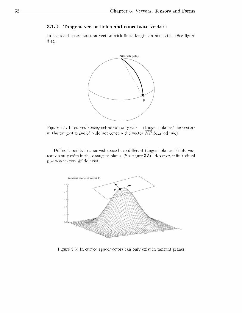
52 Chapter 3. Ve tors, Tensors and Forms3.1.2 Tangent ve tor elds and oordinate ve torsIn a urved spa e position ve tors with nite length do not exist. (See gure3.4).P

N(North pole)

Figure 3.4: In urved spa e,ve tors an only exist in tangent planes.The ve torsin the tangent plane of N,do not ontain the ve tor −−→NP (dashed line).Dierent points in a urved spa e have dierent tangent planes. Finite ve -tors do only exist in these tangent planes (See gure 3.5). However, innitesimalposition ve tors d~r do exist.P

tangent plane of point P:

Figure 3.5: In urved spa e,ve tors an only exist in tangent planes

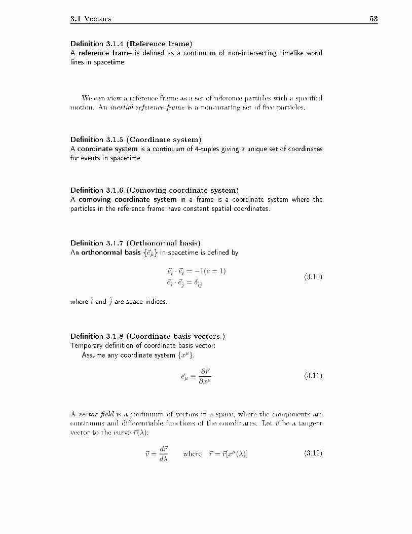
3.1 Ve tors 53Denition 3.1.4 (Referen e frame)A referen e frame is dened as a ontinuum of non-interse ting timelike worldlines in spa etime.We an view a referen e frame as a set of referen e parti les with a spe iedmotion. An inertial referen e frame is a non-rotating set of free parti les.Denition 3.1.5 (Coordinate system)A oordinate system is a ontinuum of 4-tuples giving a unique set of oordinatesfor events in spa etime.Denition 3.1.6 (Comoving oordinate system)A omoving oordinate system in a frame is a oordinate system where theparti les in the referen e frame have onstant spatial oordinates.Denition 3.1.7 (Orthonormal basis)An orthonormal basis ~eµ in spa etime is dened by~et · ~et = −1(c = 1)

~ei · ~ej = δij(3.10)where i and j are spa e indi es.Denition 3.1.8 (Coordinate basis ve tors.)Temporary denition of oordinate basis ve tor:Assume any oordinate system xµ.

~eµ ≡ ∂~r

∂xµ(3.11)A ve tor eld is a ontinuum of ve tors in a spa e, where the omponents are ontinuous and dierentiable fun tions of the oordinates. Let ~v be a tangentve tor to the urve ~r(λ):

~v =d~r

dλwhere ~r = ~r[xµ(λ)] (3.12)

54 Chapter 3. Ve tors, Tensors and FormsThe hain rule for dierentiation yields:~v =

d~r

dλ=

∂~r

∂xµdxµ

dλ=dxµ

dλ~eµ = vµ~eµ (3.13)Thus, the omponents of the tangent ve tor eld along a urve, parameterisedby λ, is given by:

vµ =dxµ

dλ(3.14)In the theory of relativity, the invariant parameter is often hosen to be theproper time. Tangent ve tor to the world line of a material parti le:

uµ =dxµ

dτ(3.15)These are the omponents of the 4-velo ity of the parti le!Digression 3.1.1 (Proper time of the photon.)Minkowski-spa e:

ds2 = −c2dt2 + dx2

= −c2dt2(1 − 1

c2(dxdt

)2)

= −(1 − v2

c2)c2dt2

(3.16)For a photon,v = c so:limv→c

ds2 = 0 (3.17)Thus, the spa etime interval between two points on the world line of a photon, iszero! This also means that the proper time for the photon is zero!! (See example3.1.2).Digression 3.1.2 (Relationships between spa etime intervals, time and proper time.)Physi al interpretation of the spa etime interval for a timelike interval:

ds2 = −c2dτ2 (3.18)where dτ is the proper time interval between two events, measured on a lo kmoving in a way, su h that it is present on both events (gure 3.6).−c2dτ2 = −c2

(1 − v2

c2)dt2

⇒ dτ =

√1 − v2

c2dt (3.19)

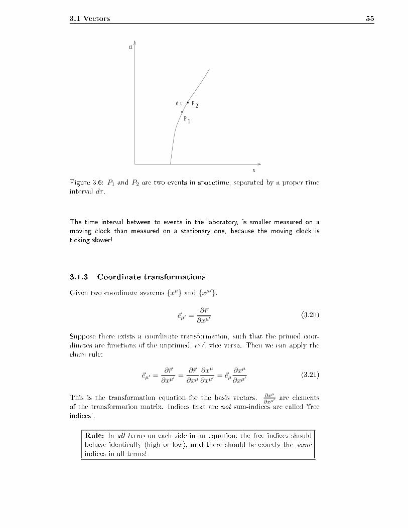
3.1 Ve tors 55

x

ct

d

P 1

P 2τ

Figure 3.6: P1 and P2 are two events in spa etime, separated by a proper timeinterval dτ .The time interval between to events in the laboratory, is smaller measured on amoving lo k than measured on a stationary one, be ause the moving lo k isti king slower!3.1.3 Coordinate transformationsGiven two oordinate systems xµ and xµ′.~eµ′ =

∂~r

∂xµ′(3.20)Suppose there exists a oordinate transformation, su h that the primed oor-dinates are fun tions of the unprimed, and vi e versa. Then we an apply the hain rule:

~eµ′ =∂~r

∂xµ′

=∂~r

∂xµ∂xµ

∂xµ′

= ~eµ∂xµ

∂xµ′

(3.21)This is the transformation equation for the basis ve tors. ∂xµ

∂xµ′ are elementsof the transformation matrix. Indi es that are not sum-indi es are alled 'freeindi es'.Rule: In all terms on ea h side in an equation, the free indi es shouldbehave identi ally (high or low), and there should be exa tly the sameindi es in all terms!

56 Chapter 3. Ve tors, Tensors and FormsApplying this rule, we an now nd the inverse transformation~eµ = ~eµ′

∂xµ′

∂xµ

~v = vµ′

~eµ′ = vµ~eµ = vµ′

~eµ∂xµ

∂xµ′So, the transformation rules for the omponents of a ve tor be omesvµ = vµ

′ ∂xµ

∂xµ′; vµ

′

= vµ∂xµ

′

∂xµ(3.22)The dire tional derivative along a urve, parametrised by λ:

d

dλ=

∂

∂xµdxµ

dλ= vµ

∂

∂xµ(3.23)where vµ = dxµ

dλ are the omponents of the tangent ve tor of the urve. Dire -tional derivative along a oordinate urve:λ = xν

∂

∂xµ∂xµ

∂xν= δµν

∂

∂xµ=

∂

∂xν(3.24)In the primed system:

∂

∂xµ′=∂xµ

∂xµ′∂

∂xµ(3.25)Denition 3.1.9 (Coordinate basis ve tors.)We dene the oordinate basis ve tors as:

~eµ =∂

∂xµ(3.26)This denition is not based upon the existen e of nite position ve tors. It appliesin urved spa es as well as in at spa es.Example 3.1.2 (Coordinate transformation)From Figure 3.7 we see that

x = r cos θ, y = r sin θ (3.27)Coordinate basis ve tors were dened by

~eµ ≡ ∂

∂xµ(3.28)

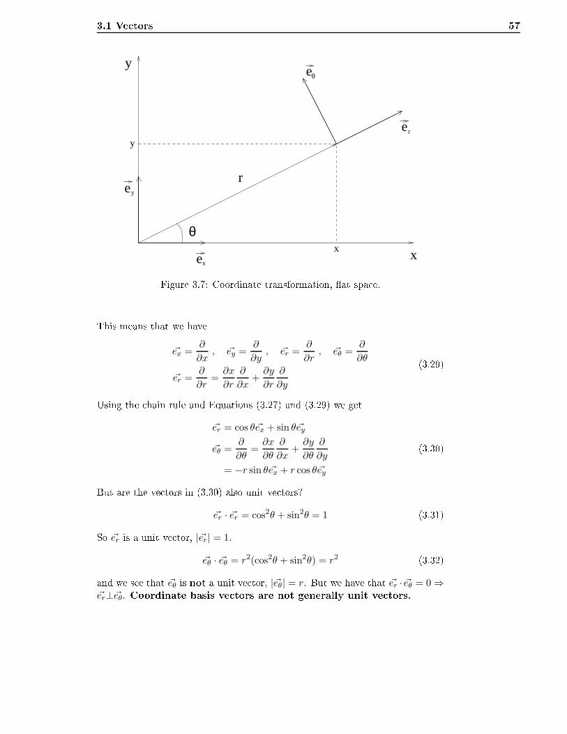
3.1 Ve tors 57y

x

y

e

er

θ

e

e

y

x

r

θ

xFigure 3.7: Coordinate transformation, at spa e.This means that we have~ex =

∂

∂x, ~ey =

∂

∂y, ~er =

∂

∂r, ~eθ =

∂

∂θ

~er =∂

∂r=∂x

∂r

∂

∂x+∂y

∂r

∂

∂y

(3.29)Using the hain rule and Equations (3.27) and (3.29) we get~er = cos θ ~ex + sin θ ~ey

~eθ =∂

∂θ=∂x

∂θ

∂

∂x+∂y

∂θ

∂

∂y

= −r sin θ ~ex + r cos θ ~ey

(3.30)But are the ve tors in (3.30) also unit ve tors?~er · ~er = cos2θ + sin2θ = 1 (3.31)So ~er is a unit ve tor, |~er| = 1.

~eθ · ~eθ = r2(cos2θ + sin2θ) = r2 (3.32)and we see that ~eθ is not a unit ve tor, |~eθ| = r. But we have that ~er · ~eθ = 0 ⇒~er⊥~eθ. Coordinate basis ve tors are not generally unit ve tors.

58 Chapter 3. Ve tors, Tensors and FormsDenition 3.1.10 (Orthonormal basis)An orthonormal basis is a ve tor basis onsisting of unit ve tors that are normal toea h other. To show that we are using an orthonormal basis we will use 'hats' overthe indi es, ~eµ.Orthonormal basis asso iated with planar polar oordinates:~er = ~er , ~eθ =

1

r~eθ (3.33)Example 3.1.3 (Relativisti Doppler Ee t)The Lorentz transformation is known from spe ial relativity and relates the referen eframes of two systems where one is moving with a onstant velo ity v with regardto the other,

x′ = γ(x− vt)

t′ = γ(t− vx

c2)A ording to the ve tor omponent transformation (3.22), the 4-momentum for aparti le moving in the x-dire tion, Pµ = (Ec , p, 0, 0) transforms as

Pµ′

=∂xµ

′

∂xµPµ,

E′ = γ(E − vp).Using the fa t that a photon has energy E = hν and momemtum p = hνc , where

h is Plan k's onstant and ν is the photon's frequen y, we get the equation for thefrequen y shift known as the relativisti Doppler ee t,ν ′ = γ(ν − v

cν) =

(1 − v

c

)ν

√(1 − v

c

) (1 + v

c

)

ν ′

ν=

√c− v

c+ v(3.34)

3.1.4 Stru ture oe ientsDenition 3.1.11 (Commutators between ve tors)The ommutator between two ve tors, ~u and ~v, is dened as[~u , ~v] ≡ ~u~v − ~v~u (3.35)

3.1 Ve tors 59where ~u~v is dened as~u~v ≡ uµ ~eµ(v

ν ~eν) = uµ∂

∂xµ(vν

∂

∂xν) (3.36)We an think of a ve tor as a linear ombination of partial derivatives. We get:

~u~v = uµ∂vν

∂xµ∂

∂xν+ uµvν

∂2

∂xµ∂xν

= uµ∂vν

∂xµ~eν + uµvν

∂2

∂xµ∂xν

(3.37)Due to the last term, ~u~v is not a ve tor.~v~u = vν

∂

∂xν(uµ

∂

∂xµ)

= vν∂uµ

∂xν~eµ + vνuµ

∂2

∂xν∂xµ

~u~v − ~v~u = uµ∂vν

∂xµ~eν − vν

∂uµ

∂xν~eµ

︸ ︷︷ ︸vµ ∂uν

∂xµ ~eν

= (uµ∂vν

∂xµ− vµ

∂uν

∂xµ)~eν

(3.38)Here we have used that

∂2

∂xµ∂xν=

∂2

∂xν∂xµ(3.39)The Einstein omma notation ⇒

~u~v − ~v~u = (uµvν,µ − vµuν,µ)~eν (3.40)As we an see, the ommutator between two ve tors is itself a ve tor.Denition 3.1.12 (Stru ture oe ients cρ

µν)The stru ture oe ients cρµν in an arbitrary basis ~eµ are dened by:

[ ~eµ , ~eν ] ≡ cρµν ~eρ (3.41)Stru ture oe ients in a oordinate basis:[ ~eµ , ~eν ] = [

∂

∂xµ,∂

∂xν]

=∂

∂xµ(∂

∂xν) − ∂

∂xν(∂

∂xµ)

=∂2

∂xµ∂xν− ∂2

∂xν∂xµ= 0

(3.42)

60 Chapter 3. Ve tors, Tensors and FormsThe ommutator between two oordinate basis ve tors is zero, so the stru ture oe ients are zero in oordinate basis.Example 3.1.4 (Stru ture oe ients in planar polar oordinates)We will nd the stru ture oe ients of an orthonormal basis in planar polar oor-dinates. In (3.33) we found that~er = ~er , ~eθ =

1

r~eθ (3.43)We will now use this to nd the stru ture oe ients.

[~er , ~eθ] = [∂

∂r,

1

r

∂

∂θ]

=∂

∂r(1

r

∂

∂θ) − 1

r

∂

∂θ(∂

∂r)

= − 1

r2∂

∂θ+

1

r

∂2

∂r∂θ− 1

r

∂2

∂θ∂r

= − 1

r2~eθ = −1

r~eθ

(3.44)To nd the stru ture oe ients in an orthonormal basis we must use [~er , ~eθ] =−1r~eθ.

[~eµ , ~eν ] = cρµν~eρ (3.45)Using (3.44) and (3.45) we getcθrθ

= −1

r(3.46)From the denition of cρµν ([~u , ~v] = −[~v , ~u]) we see that the stru ture oe ientsare anti symmetri in their lower indi es:

cρµν = −cρνµ (3.47)cθθr

=1

r= −cθ

rθ(3.48)3.2 TensorsA 1-form-basis ω1, . . ., ωn is dened by:

ωµ(~eν) = δµν (3.49)

3.2 Tensors 61An arbitrary 1-form an be expressed, in terms of its omponents, as a linear ombination of the basis forms:α = αµω

µ (3.50)where αµ are the omponents of α in the given basis.Using eqs.(3.49) and (3.50), we nd:α(~eν) = αµω

µ(~eν) = αµδµν = αν

α(~v) = α(vµ~eµ) = vµα(~eµ) = vµαµ = v1α1 + v2α2 + . . .(3.51)We will now look at fun tions of multiple variables.Denition 3.2.1 (Multilinear fun tion, tensors)A multilinear fun tion is a fun tion that is linear in all its arguments and maps one-forms and ve tors into real numbers. A tensor is a multilinear fun tion that mapsone-forms and ve tors into real numbers.

• A ovariant tensor only maps ve tors.• A ontravariant tensor only maps forms.• A mixed tensor maps both ve tors and forms into R.A tensor of rank (NN ′

) maps N one-forms and N ′ ve tors into R. It is usual tosay that a tensor is of rank (N +N ′). A one-form, for example, is a ovarianttensor of rank 1:α(~v) = vµαµ (3.52)Denition 3.2.2 (Tensor produ t)The basis of a tensor R of rank q ontains a tensor produ t, ⊗. If T and S aretwo tensors of rank m and n, the tensor produ t is dened by:

T ⊗ S( ~u1,..., ~um, ~v1,..., ~vn) ≡ T ( ~u1,..., ~um)S(~v1,..., ~vn) (3.53)where T and S are tensors of rank m and n, respe tively. T ⊗S is a tensor of rank(m+ n).Let R = T ⊗ S. We then have

R = Rµ1,...,µqωµ1 ⊗ ωµ2 ⊗ · · · ⊗ ωµq (3.54)

62 Chapter 3. Ve tors, Tensors and FormsNoti e that S ⊗ T 6= T ⊗ S. We get the omponents of a tensor (R) by usingthe tensor on the basis ve tors:Rµ1,...,µq = R( ~eµ1 ,..., ~eµq ) (3.55)The indi es of the omponents of a ontravariant tensor are written as upperindi es, and the indi es of a ovariant tensor as lower indi es.Example 3.2.1 (Example of a tensor)Let ~u and ~v be two ve tors and α and β two 1-forms.

~u = uµ~eµ; ~v = vµ~eµ; α = αµωµ; β = βµω

µ (3.56)From these we an onstru t tensors of rank 2 through the relation R = ~u ⊗ ~v asfollows: The omponents of R areRµ1µ2 = R(ωµ1 , ωµ2)

= ~u⊗ ~v(ωµ1 , ωµ2)

= ~u(ωµ1)~v(ωµ2)

= uµ~eµ(ωµ1)vν~eν(ω

µ2)

= uµδµ1µ v

νδµ2ν

= uµ1vµ2

(3.57)3.2.1 Transformation of tensor omponentsWe shall not limit our dis ussion to oordinate transformations. Instead, wewill onsider arbitrary transformations between bases, ~eµ −→

~eµ′. Theelements of transformation matri es are denoted by Mµ

µ′ su h that~eµ′ = ~eµM

µµ′ and ~eµ = ~eµ′M

µ′µ (3.58)where Mµ′

µ are elements of the inverse transformation matrix. Thus, it followsthatMµ

µ′Mµ′

ν = δµν (3.59)If the transformation is a oordinate transformation, the elements of the matrixbe omeMµ′

µ =∂xµ

′

∂xµ(3.60)

3.2 Tensors 633.2.2 Transformation of basis 1-formsωµ

′

= Mµ′µω

µ

ωµ = Mµµ′ω

µ′(3.61)The omponents of a tensor of higher rank transform su h that every on-travariant index (upper) transforms as a basis 1-form and every ovariant index(lower) as a basis ve tor. Also, all elements of the transformation matrix aremultiplied with one another.Example 3.2.2 (A mixed tensor of rank 3)

Tα′

µ′ν′ = Mα′

αMµµ′M

νν′T

αµν (3.62)The omponents in the primed basis are linear ombinations of the omponentsin the unprimed basis.Tensor transformation of omponents means that tensors have a basis in-dependent existen e. That is, if a tensor has non-vanishing omponents in agiven basis then it has non-vanishing omponents in all bases. This meansthat tensor equations have a basis independent form. Tensor equations areinvariant. A basis transformation might result in the vanishing of one or moretensor omponents. Equations in omponent form may dier from one basis toanother. But an equation expressed in tensor omponents an be transformedfrom one basis to another using the tensor omponent transformation rules. Anequation that is expressed only in terms of tensor omponents is said to be ovariant.3.2.3 The metri tensorDenition 3.2.3 (The metri tensor)The s alar produ t of two ve tors ~u and ~v is denoted by g(~u,~v) and is dened asa symmetri linear mapping whi h for ea h pair of ve tors gives a s alar g(~v,~u) =g(~u,~v).The value of the s alar produ t g(~u,~v) is given by spe ifying the s alarprodu ts of ea h pair of basis-ve tors in a basis.g is a symmetri ovariant tensor of rank 2. This tensor is known as the

64 Chapter 3. Ve tors, Tensors and Formsmetri tensor. The omponents of this tensor areg(~eµ, ~eν) = g µν (3.63)

~u · ~v = g(~u,~v) = g(uµ~eµ, vν~eν) = uµvνg(~eµ, ~eν) = uµuνg µν (3.64)Usual notation:

~u · ~v = g µνuµvν (3.65)The absolute value of a ve tor:

|~v| =√g(~v,~v) =

√|g µνvµvν | (3.66)Example 3.2.3 (Cartesian oordinates in a plane)

~ex · ~ex = 1, ~ey · ~ey = 1, ~ex · ~ey = ~ey · ~ex = 0

g xx = g yy = 1, g xy = g yx = 0 (3.67)g µν =

(1 00 1

)

Example 3.2.4 (Basis-ve tors in plane polar- oordinates)~er · ~er = 1, ~eθ · ~eθ = r2, ~er · ~eθ = 0, (3.68)The metri tensor in plane polar- oordinates:

g µν =

(1 00 r2

) (3.69)Example 3.2.5 (Non-diagonal basis-ve tors)~e1 · ~e1 = 1, ~e2 · ~e2 = 1, ~e1 · ~e2 = cos θ = ~e2 · ~e1

g µν =

(1 cos θ

cos θ 1

)=

(g 11 g 12

g 21 g 22

) (3.70)

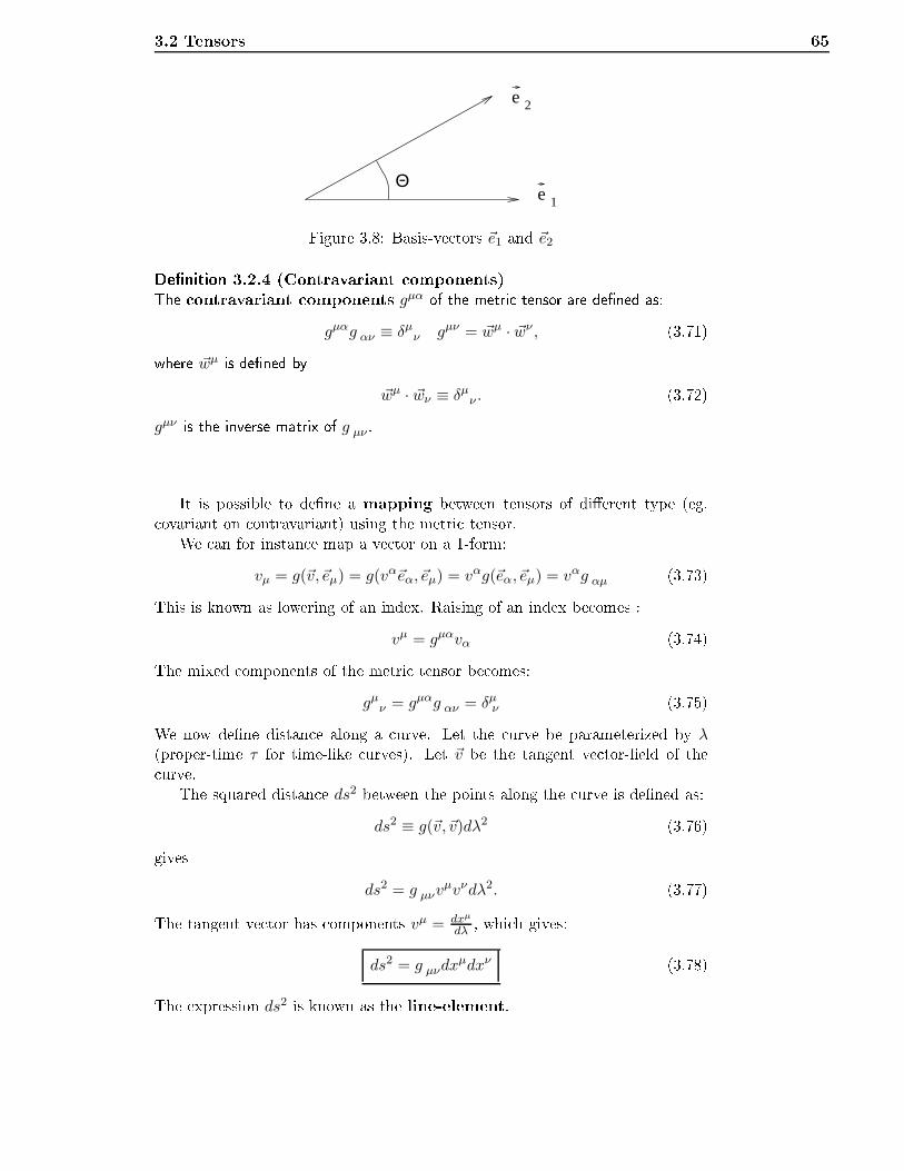
3.2 Tensors 65e 1

2e

ΘFigure 3.8: Basis-ve tors ~e1 and ~e2Denition 3.2.4 (Contravariant omponents)The ontravariant omponents gµα of the metri tensor are dened as:gµαg αν ≡ δµν gµν = ~wµ · ~wν , (3.71)where ~wµ is dened by

~wµ · ~wν ≡ δµν . (3.72)gµν is the inverse matrix of g µν .It is possible to dene a mapping between tensors of dierent type (eg. ovariant on ontravariant) using the metri tensor.We an for instan e map a ve tor on a 1-form:

vµ = g(~v,~eµ) = g(vα~eα, ~eµ) = vαg(~eα, ~eµ) = vαg αµ (3.73)This is known as lowering of an index. Raising of an index be omes :vµ = gµαvα (3.74)The mixed omponents of the metri tensor be omes:

gµν = gµαg αν = δµν (3.75)We now dene distan e along a urve. Let the urve be parameterized by λ(proper-time τ for time-like urves). Let ~v be the tangent ve tor-eld of the urve.The squared distan e ds2 between the points along the urve is dened as:ds2 ≡ g(~v,~v)dλ2 (3.76)givesds2 = g µνv

µvνdλ2. (3.77)The tangent ve tor has omponents vµ = dxµ

dλ , whi h gives:ds2 = g µνdx

µdxν (3.78)The expression ds2 is known as the line-element.

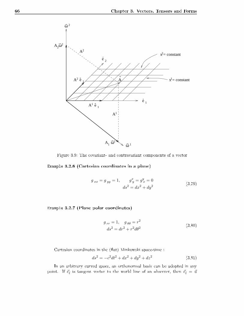
66 Chapter 3. Ve tors, Tensors and Forms

x = constant

x = constant

1

2

A

A ω22

A e

e

22

2

ω 2

A2

1A e1 1e

1A

A ω11 ω 1Figure 3.9: The ovariant- and ontravariant omponents of a ve torExample 3.2.6 (Cartesian oordinates in a plane)

g xx = g yy = 1, gxy = gyx = 0

ds2 = dx2 + dy2(3.79)

Example 3.2.7 (Plane polar oordinates)g rr = 1, g θθ = r2

ds2 = dr2 + r2dθ2(3.80)

Cartesian oordinates in the (at) Minkowski spa e-time :ds2 = −c2dt2 + dx2 + dy2 + dz2 (3.81)In an arbitrary urved spa e, an orthonormal basis an be adopted in anypoint. If ~et is tangent ve tor to the world line of an observer, then ~et = ~u

3.3 Forms 67where ~u is the 4-velo ity of the observer. In this ase, we are using what we allthe omoving orthonormal basis of the observer. In a su h basis, we have theMinkowski-metri :ds2 = ηµνdx

µdxν (3.82)3.3 FormsAn antisymmetri tensor is a tensor whose sign hanges under an arbitraryex hange of two arguments.A(· · · , ~u, · · · , ~v, · · · ) = −A(· · · , ~v, · · · , ~u, · · · ) (3.83)The omponents of an antisymmetri tensor hange sign under ex hange oftwo indi es.

A···µ···ν··· = −A···ν···µ··· (3.84)Denition 3.3.1 (p-form)A p-form is dened to be an antisymmetri , ovariant tensor of rank p.An antisymmetri tensor produ t ∧ is dened by:ω[µ1 ⊗ · · · ⊗ ωµp] ∧ ω[ν1 ⊗ · · · ⊗ ωνq] ≡ (p+ q)!

p!q!ω[µ1 ⊗ · · · ⊗ ωνq] (3.85)where [ denotes antisymmetri ombinations dened by:

ω[µ1 ⊗ · · · ⊗ ωµp] ≡ 1

p!· (the sum of terms withall possible permutationsof indi es with, + for evenand - for odd permutations) (3.86)

Example 3.3.1 (antisymmetri ombinations)ω[µ1 ⊗ ωµ2] =

1

2(ωµ1 ⊗ ωµ2 − ωµ2 ⊗ ωµ1) (3.87)

68 Chapter 3. Ve tors, Tensors and FormsExample 3.3.2 (antisymmetri ombinations)ω[µ1 ⊗ ωµ2 ⊗ ωµ3] =

1

3!(ωµ1 ⊗ ωµ2 ⊗ ωµ3 + ωµ3 ⊗ ωµ1 ⊗ ωµ2 + ωµ2 ⊗ ωµ3 ⊗ ωµ1

− ωµ2 ⊗ ωµ1 ⊗ ωµ3 − ωµ3 ⊗ ωµ2 ⊗ ωµ1 − ωµ1 ⊗ ωµ3 ⊗ ωµ2)

=1

3!ǫijk(ω

µi ⊗ ωµj ⊗ ωµk) (3.88)Example 3.3.3 (A 2-form in 3-spa e)α = α12ω

1⊗ω2+α21ω2⊗ω1+α13ω

1⊗ω3+α31ω3⊗ω1+α23ω

2⊗ω3+α32ω3⊗ω2(3.89)Now the antisymmetry of α means that

+α21 = −α12; +α31 = −α13; +α32 = −α23 (3.90)α =α12(ω

1 ⊗ ω2 − ω2 ⊗ ω1)

+ α13(ω1 ⊗ ω3 − ω3 ⊗ ω1)

+ α23(ω2 ⊗ ω3 − ω3 ⊗ ω2)

= α|µν|2ω[µ ⊗ ων]

(3.91)where |µν| means summation only for µ < ν (see (Misner, Thorne and Wheeler1973)). We now use the denition of ∧ with p = q = 1. This givesα = α|µν|ω

µ ∧ ων

ωµ∧ ων is theform basis. We an also write

α =1

2αµνω

µ ∧ ων

A tensor of rank 2 an always be split up into a symmetri and an anti-symmetri part. (Note that tensors of higher rank an not be split up in thisway.)Tµν =

1

2(Tµν − Tνµ) +

1

2(Tµν + Tνµ)

= Aµν + Sµν

(3.92)

3.3 Forms 69We thus have:SµνA

µν =1

4(Tµν + Tνµ)(T

µν − T νµ)

=1

4(TµνT

µν − TµνTνµ + TνµT

µν − TνµTνµ)

= 0

(3.93)In general, summation over indi es of a symmetri and an antisymmetri quan-tity vanishes. In a summation TµνAµν where Aµν is antisymmetri and Tµν hasno symmetry, only the antisymmetri part of Tµν ontributes. So that, inα =

1

2αµνω

µ ∧ ων (3.94)only the antisymmetri elements ανµ = −αµν , ontribute to the summation.These antisymmetri elements are the form omponentsForms are antisymmetri ovariant tensors. Be ause of this antisymmetrya form with two identi al omponents must be a null form (= zero). e.g.α131 = −α131 ⇒ α131 = 0In an n-dimensional spa e all p-forms with p > n are null forms.

70 Chapter 3. Ve tors, Tensors and FormsProblems3.1. 1-forms(a) Show that the following holds:p(Aα~eα) = Aαp(~eα) (3.95)(b) Let the omponents of p, ~A and ~B be (−1, 1, 2, 0), (2, 1, 0,−1) and (0, 2, 0, 0),respe tively. Find (i) p( ~A); (ii) p( ~B); (iii) p( ~A− 3 ~B); (iv) p( ~A) − 3p( ~B).3.2. The tensor produ t(a) Given one-forms α and β. Assume that the omponents of α and β are

(1, 1, 0, 0) and (−1, 0, 1, 0), respe tively. Show by using two ve tors asarguments that α ⊗ β 6= β ⊗ α . Find also the omponents of α ⊗ β.(b) Find also the omponents of the symmetri and anti-symmetri part ofα ⊗ β, dened above.3.3. The wedge produ tGiven the following forms in a 4-dimensional spa etime:

α = αµωµ

β = βµνωµ ∧ ων

γ = γµωµ

δ = δµνωµ ∧ ων (3.96)What is the orrespondan e between

α ∧ β og β ∧ α ,

α ∧ γ og γ ∧ α ,

β ∧ δ og δ ∧ β ?

(3.97)3.4. Contra tions of tensorsAssume that A is an anti-symmetri tensor of rank (20) , B a symmetri tensorof rank (02), C an arbitrary tensor of rank (02), and D an arbitrary tensor ofrank (20). Show thatAabBab = 0,

AabCab = AabC[ab],andBabD

ab = BabD(ab).

Problems 713.5. Symmetri and anti-symmetri tensors(a) Let the omponents of the tensor Mαβ be given by the matrix

0 1 0 01 −1 0 22 0 0 11 0 −2 0

(3.98)Find (let the metri tensor have omponents ηαβ = diag(−1, 1, 1, 1)):1. the omponents of the symmetri tensorM (αβ) and the antisymmetri tensor M [αβ];2. the omponents of Mαβ;3. the omponents of M βα ;4. the omponents of Mαβ .(b) Consider now the tensor with omponentsMα

β. Does it make sen e to talkabout the symmetri and antisymmetri parts of this tensor? If yes, denethem. If no, explain why.3.6. Four-ve tors(a) Given three four-ve tors:A = 4et + 3ex + 2ey + ez

B = 5et + 4ex + 3ey

C = et + 2ex + 3ey + 4ez,whereex · ex = ey · ey = ez · ez = 1,while

et · et = −1.Show that A is time-like, B is light-like and C is spa e-like.(b) Assume that A and B are two non-zero orthogonal four-ve tors, A ·B = 0.Show the following:•If A is time-like, then B is spa e-like.•If A is light-like, then B is spa e-like or light-like.•If A and B is light-like, then they are proportional.•If A is spa e-like, then B is time-like, light-like or spa e-like.Illustrate this in a three-dimensional Minkowski-diagram.( ) A hange of basis is given by

et′ = cosh aet + sinhaex

ex′ = sinhaet + cosh aex

ey′ = ey, ez′ = ez.

72 Chapter 3. Ve tors, Tensors and FormsShow that this des ribes a Lorentz-transformation along the x-axis, wherethe relative velo ity v between the referen e frames, are given by v =tanh a. Draw the ve tors in a two-dimensional Minkowski-diagram andnd what type of urves the et′ and ex′ des ribe as a varies.(d) The three-ve tor v des ribing the velo ity of a parti le is dened with re-spe t to an observer. Explain why the four-velo ity u is dened independentof any observer.The four-momentum of a parti le, with rest mass m, is dened by p =mu = mdr/dτ , where τ is the o-moving time of the parti le. Show thatp is time-like, and that p · p = −m2. Draw, in a Minkowski-diagram, the urve to whi h p must be tangent to, and explain how this is altered asm −→ 0.Assume that the energy of the parti le is being observed by an observerwith four-velo ity u. Show that the energy he measures is given by

E = −p · u. (3.99)This is an expression whi h is very useful when one wants to al ulate theenergy of a parti le in an arbitrary referen e frame.3.7. Wedge produ ts of formsGiven the one-formsa = x2ω1 − yω2, b = yω1 − xzω2 + y2ω3, σ = y2zω2,the two-form

η = xyω1 ∧ ω3 + xω2 ∧ ω3,and the three-formθ = xyzω1 ∧ ω2 ∧ ω3.Cal ulate the wedge produ ts

a ∧ b, a ∧ b ∧ σ, a ∧ η, a ∧ θ.3.8. Coordinate-transformations in a two-dimensional Eu lidean planeIn this problem we will investigate ve tors x in the two-dimensional Eu lideanplane E2. The set em|m = x, y is an orthonormal basis in E2, i.e.em · en = δmn.The omponents of a ve tor x in this basis is given by x and y, or xm:

x = xmem = xex + yey.A skew basis set, eµ|µ = 1, 2, is also given. In this basisx = xµeµ = x1e1 + x2e2.The transformation between these to oordinates are

x1 = 2x− y,

x2 = x+ y.

Problems 73(a) Find e1 and e2 expressed in terms of ex and ey. Determine the transfor-mation matrix M, dened byxm = Mm

µxµ.What is M

−1?(b) The metri tensor g is given byds2 = gµνdx

µdxν = gmndxmdxn,where ds is the distan e between x and x + dx. Show that we have

eµ · eν = gµν .What is the relation between the matri es (gµν) and (gmn) and the trans-formation matrix M?The s alar produ t between two ve tors an therefore be expressed asv · u = gµνv

µuν = gmnvmun.Verify this equation for the ase u = 2e1 and v = 3e2.( ) Using the basis ve tors eµ, we an dene a new set ωµ by

ωµ · eν = δµν .Find ω1 and ω2 expressed in terms of ex and ey. Why is ωm = em, whileωµ 6= eµ?A ve tor x an now be expressed as

x = xµeµ = xµωµ.What is the relation between the ontravariant omponents xµ and the ovariant omponents xµ? Determine both set of omponents for the ve tor

A = 3ex + ey.In a (x, y)-diagram, draw the the three set of basis ve tors eµ, em andωµ. What is the geometri al interpretation of the relation between thetwo sets eµ and ωµ? Depi t also the ve tor A and explain how the omponents of A in the three basis sets an be seen from the diagram.(d) Find the matrix (gµν) dened by

ωµ · ων = gµν .Verify that this matrix is the inverse to (gµν).The metri tensor is a symmetri tensor of rank 2, and an therefore beexpressed with the basis ve tors em⊗ en in the tensor produ t spa e E2 ⊗E2,

g = gmnem ⊗ en.

74 Chapter 3. Ve tors, Tensors and FormsShow that we also an express it asg = gµνω

µ ⊗ ων ,andg = gµνeµ ⊗ eν .What is the dimension of the spa e spanned by the ve tors em ⊗ en?The antisymmetri tensors span a one-dimensional subspa e. Show this byshowing that an antisymmetri tensor Amn is a linear ombination of thebasis ve tor

ex ∧ ey = ex ⊗ ey − ey ⊗ exFind u ∧ v where u and v are the ve tors from (b), expressed in terms ofthe basis ve tor ex ∧ ey. What is the relation between this and the areathat is spanned by u and v? Cal ulate also ω1 ∧ ω2

Chapter 4A elerated Referen e Frames4.1 Rotating referen e frames4.1.1 The spatial metri tensorLet ~e0 be the 4-velo ity eld (x0 = ct, c = 1, x0 = t) of the referen e parti lesin a referen e frame R. We are going to nd the metri tensor γij in a tangentspa e orthogonal to ~e0, expressed by the metri tensor gµν of spa etime.In an arbitrary oordinate basis ~eµ, ~ei is not ne essarily orthogonal to~e0. We hoose ~e0‖~e0. Let ~e⊥i be the omponent of ~ei orthogonal to ~e0, thatis:~e⊥i · ~e0 = 0. The metri tensor of spa e is dened by:

γij = ~e⊥i · ~e⊥j , γi0 = 0, γ00 = 0

~e⊥i = ~ei − ~e‖i

~e‖i =~ei · ~e0~e0 · ~e0

~e0 =gi0g00

~e0

γij = (~ei − ~e‖i) · (~ej − ~e‖j)

= (~ei −gi0g00

~e0) · (~ej −gj0g00

~e0)

= ~ei · ~ej −gj0g00

~e0 · ~ei −gi0g00

~e0 · ~ej +gi0gj0g200

~e0 · ~e0

= gij −gi0gj0g00

− gi0gj0g00

+gi0gj0g00

⇒ γij = gij −gi0gj0g00

(4.1)(Note:gij = gji ⇒ γij = γji)The line element in spa e:dl2 = γijdx

idxj =(gij −

gi0gj0g00

)dxidxj (4.2)gives the distan e between simultaneous events in a referen e frame where themetri tensor of spa etime in a omoving oordinate system is gµν .75

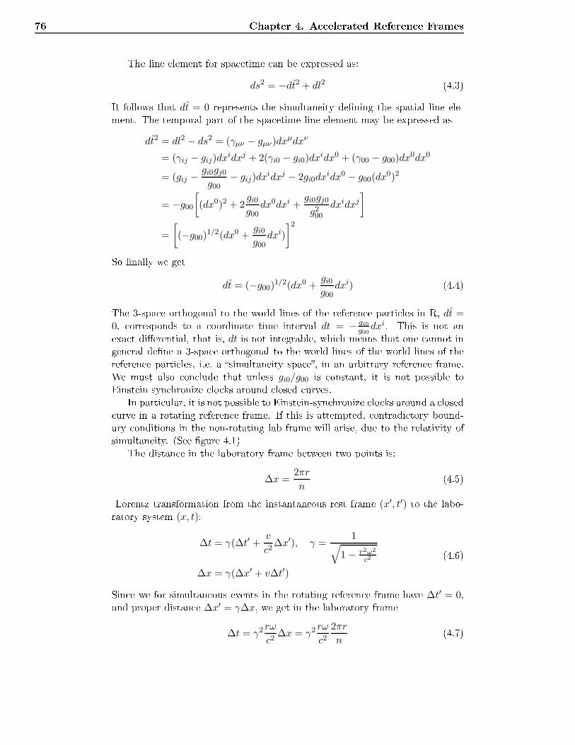
76 Chapter 4. A elerated Referen e FramesThe line element for spa etime an be expressed as:ds2 = −dt2 + dl2 (4.3)It follows that dt = 0 represents the simultaneity dening the spatial line ele-ment. The temporal part of the spa etime line element may be expressed as

dt2 = dl2 − ds2 = (γµν − gµν)dxµdxν

= (γij − gij)dxidxj + 2(γi0 − gi0)dx

idx0 + (γ00 − g00)dx0dx0

= (gij −gi0gj0g00

− gij)dxidxj − 2gi0dx

idx0 − g00(dx0)2

= −g00[(dx0)2 + 2

gi0g00

dx0dxi +gi0gj0g200

dxidxj]

=

[(−g00)1/2(dx0 +

gi0g00

dxi)

]2So nally we getdt = (−g00)1/2(dx0 +

gi0g00

dxi) (4.4)The 3-spa e orthogonal to the world lines of the referen e parti les in R, dt =0, orresponds to a oordinate time interval dt = − gi0

g00dxi. This is not anexa t dierential, that is, dt is not integrable, whi h means that one annot ingeneral dene a 3-spa e orthogonal to the world lines of the world lines of thereferen e parti les, i.e. a simultaneity spa e, in an arbitrary referen e frame.We must also on lude that unless gi0/g00 is onstant, it is not possible toEinstein syn hronize lo ks around losed urves.In parti ular, it is not possible to Einstein-syn hronize lo ks around a losed urve in a rotating referen e frame. If this is attempted, ontradi tory bound-ary onditions in the non-rotating lab frame will arise, due to the relativity ofsimultaneity. (See gure 4.1)The distan e in the laboratory frame between two points is:

∆x =2πr

n(4.5)Lorentz transformation from the instantaneous rest frame (x′, t′) to the labo-ratory system (x, t):

∆t = γ(∆t′ +v

c2∆x′), γ =

1√1 − r2ω2

c2

∆x = γ(∆x′ + v∆t′)

(4.6)Sin e we for simultaneous events in the rotating referen e frame have ∆t′ = 0,and proper distan e ∆x′ = γ∆x, we get in the laboratory frame∆t = γ2 rω

c2∆x = γ2 rω

c22πr

n(4.7)

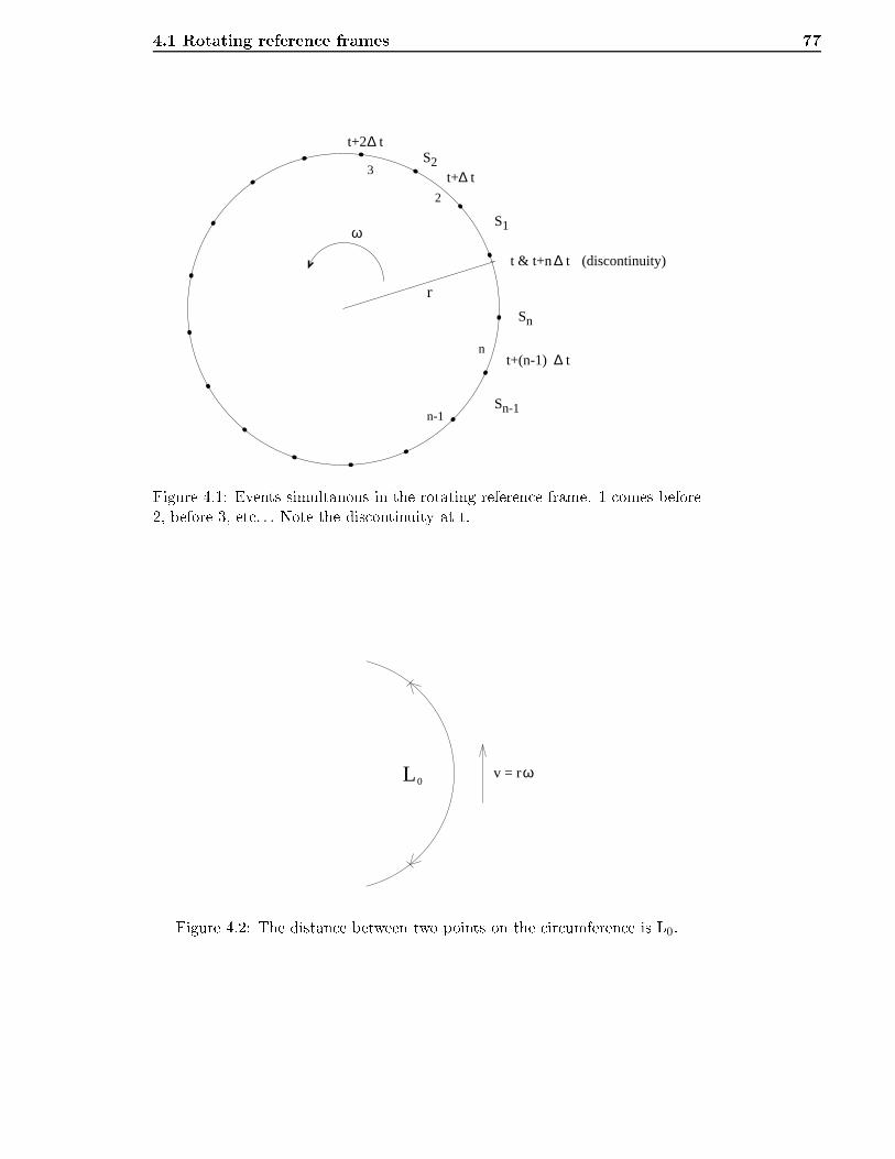
4.1 Rotating referen e frames 77

r

t & t+n ∆ t

t+2∆ t

t+∆ t

t+(n-1) ∆ t

S

S

S

S3

n-1

n

1

2

2

n

ω

(discontinuity)

n-1Figure 4.1: Events simultanous in the rotating referen e frame. 1 omes before2, before 3, et . . . Note the dis ontinuity at t.

0L v = rω

Figure 4.2: The distan e between two points on the ir umferen e is L0.

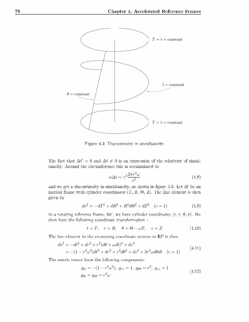
78 Chapter 4. A elerated Referen e FramesT = t = constant

T = t = constant

θ = constant

t = constant

Figure 4.3: Dis ontinuity in simultaneity.The fa t that ∆t′ = 0 and ∆t 6= 0 is an expression of the relativity of simul-taneity. Around the ir umferen e this is a umulated ton∆t = γ2 2πr2ω

c2(4.8)and we get a dis ontinuity in simultaneity, as shown in gure 4.3. Let IF be aninertial frame with ylinder oordinates (T, R, Θ, Z). The line element is thengiven by

ds2 = −dT 2 + dR2 +R2dΘ2 + dZ2 (c = 1) (4.9)In a rotating referen e frame, RF, we have ylinder oordinates (t, r, θ, z). Wethen have the following oordinate transformation :t = T, r = R, θ = Θ − ωT, z = Z (4.10)The line element in the o-moving oordinate system in RF is then

ds2 = −dt2 + dr2 + r2(dθ + ωdt)2 + dz2

= −(1 − r2ω2)dt2 + dr2 + r2dθ2 + dz2 + 2r2ωdθdt (c = 1)(4.11)The metri tensor have the following omponents:

gtt = −(1 − r2ω2), grr = 1, gθθ = r2, gzz = 1

gθt = gtθ = r2ω(4.12)

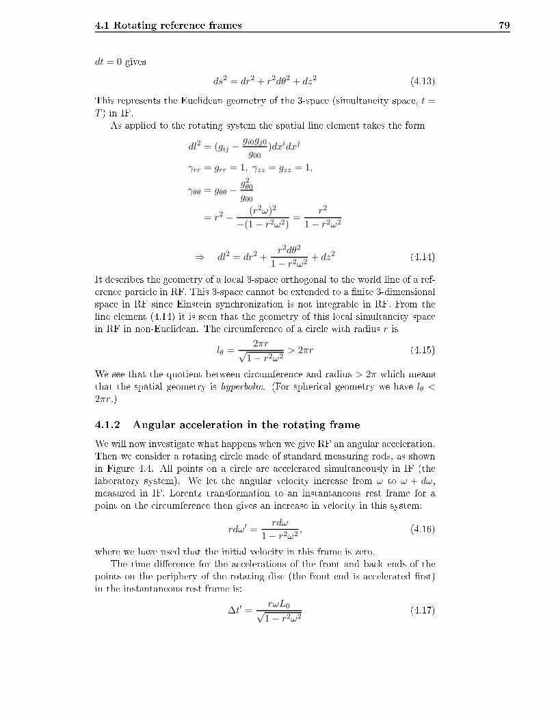
4.1 Rotating referen e frames 79dt = 0 gives

ds2 = dr2 + r2dθ2 + dz2 (4.13)This represents the Eu lidean geometry of the 3-spa e (simultaneity spa e, t =T ) in IF.As applied to the rotating system the spatial line element takes the form

dl2 = (gij −gi0gj0g00

)dxidxj

γrr = grr = 1, γzz = gzz = 1,

γθθ = gθθ −g2θ0

g00

= r2 − (r2ω)2

−(1 − r2ω2)=

r2

1 − r2ω2

⇒ dl2 = dr2 +r2dθ2

1 − r2ω2+ dz2 (4.14)It des ribes the geometry of a lo al 3-spa e orthogonal to the world line of a ref-eren e parti le in RF. This 3-spa e annot be extended to a nite 3-dimensionalspa e in RF sin e Einstein syn hronization is not integrable in RF. From theline element (4.14) it is seen that the geometry of this lo al simultaneity spa ein RF in non-Eu lidean. The ir umferen e of a ir le with radius r is

lθ =2πr√

1 − r2ω2> 2πr (4.15)We see that the quotient between ir umferen e and radius > 2π whi h meansthat the spatial geometry is hyperboli . (For spheri al geometry we have lθ <

2πr.)4.1.2 Angular a eleration in the rotating frameWe will now investigate what happens when we give RF an angular a eleration.Then we onsider a rotating ir le made of standard measuring rods, as shownin Figure 4.4. All points on a ir le are a elerated simultaneously in IF (thelaboratory system). We let the angular velo ity in rease from ω to ω + dω,measured in IF. Lorentz transformation to an instantaneous rest frame for apoint on the ir umferen e then gives an in rease in velo ity in this system:rdω′ =

rdω

1 − r2ω2, (4.16)where we have used that the initial velo ity in this frame is zero.The time dieren e for the a elerations of the front and ba k ends of thepoints on the periphery of the rotating dis (the front end is a elerated rst)in the instantaneous rest frame is:

∆t′ =rωL0√1 − r2ω2

(4.17)

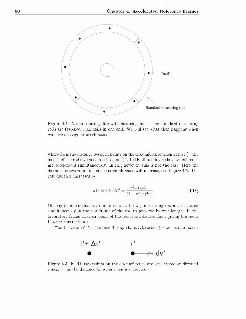
80 Chapter 4. A elerated Referen e Frames

"nail"

Standard measuring rodFigure 4.4: A non-rotating dis with measring rods. The standard measuringrods are fastened with nails in one end. We will see what then happens whenwe have an angular a eleration.where L0 is the distan e between points on the ir umferen e when at rest (= thelength of the rods when at rest), L0 = 2πrn . In IF all points on the ir umferen eare a elerated simultaneously. In RF, however, this is not the ase. Here thedistan e between points on the ir umferen e will in rease, see Figure 4.5. Therest distan e in reases by

dL′ = rdω′∆t′ =r2ωL0dω

(1 − r2ω2)3/2. (4.18)(It may be noted that ea h point on an arbitrary measuring rod is a eleratedsimultaneously in the rest frame of the rod to preserve its rest length. In thelaboratory frame the rear point of the rod is a elerated rst, giving the rod aLorentz ontra tion.)The in rease of the distan e during the a eleration (in an instantaneous

∆ t’ t’dv’

t’+ Figure 4.5: In RF two points on the ir umferen e are a elerated at dierenttimes. Thus the distan e between them is in reased.

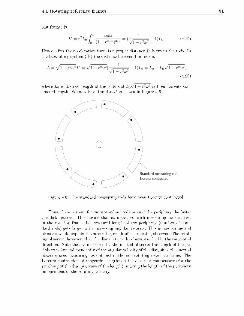
4.1 Rotating referen e frames 81rest frame) isL′ = r2L0

∫ ω

0

ωdω

(1 − r2ω2)3/2= (

1√1 − r2ω2

− 1)L0. (4.19)Hen e, after the a eleration there is a proper distan e L′ between the rods. Inthe laboratory system (IF) the distan e between the rods isL =

√1 − r2ω2L′ =

√1 − r2ω2(

1√1 − r2ω2

− 1)L0 = L0 − L0

√1 − r2ω2,(4.20)where L0 is the rest length of the rods and L0

√1 − r2ω2 is their Lorentz on-tra ted length. We now have the situation shown in Figure 4.6.

Lorenz contractedStandard measuring rod,Figure 4.6: The standard measuring rods have been Lorentz ontra ted.Thus, there is room for more standard rods around the periphery the fasterthe disk rotates. This means that as measured with measuring rods at restin the rotating frame the measured length of the periphery (number of stan-dard rods) gets larger with in reasing angular velo ity. This is how an inertialobserver would explain the measuring result of the rotating observer. The rotat-ing observer, however, that the dis material has been stre hed in the tangentialdire tion. Note that as measured by the inertial observer the length of the pe-riphery is 2πr independently of the angular velo ity of the dis , sin e the inertialobserver uses measuring rods at rest in the non-rotating referen e frame. TheLorentz ontra tion of tangential lengths on the dis just ompensates for thestre hing of the dis (in rease of the length), making the length of the peripheryindependent of the rotating velo ity.

82 Chapter 4. A elerated Referen e Frames4.1.3 Gravitational time dilationds2 = −(1 − r2ω2

c2)c2dt2 + dr2 + r2dθ2 + dz2 + 2r2ωdθdt (4.21)We now look at standard lo ks with onstant r and z.

ds2 = c2dt2[−(1 − r2ω2

c2) +

r2

c2(dθ

dt)2 + 2

r2ω

c2dθ

dt] (4.22)Let dθ

dt ≡ θ be the angular velo ity of the lo k in RF. The proper time intervalmeasured by the lo k is thends2 = −c2dτ2 (4.23)From this we see that

dτ = dt

√

1 − r2ω2

c2− r2θ2

c2− 2

r2ωθ

c2(4.24)A non-moving standard lo k in RF: θ = 0 ⇒

dτ = dt

√1 − r2ω2

c2(4.25)Seen from IF, the non-rotating laboratory system, (4.25) represents the velo itydependent time dilation from the spe ial theory of relativity.But how is (4.25) interpreted in RF? The lo k does not move relative toan observer in this system, hen e what happens an not bee interpreted as avelo ity dependent phenomenon. A ording to Einstein, the fa t that standard lo ks slow down the farther away from the axis of rotation they are, is due toa gravitational ee t.We will now nd the gravitational potential at a distan e r from the axis.The sentripetal a eleration is v2/r, v = rω so:

Φ = −∫ r

0g(r)dr = −

∫ r

0rω2dr = −1

2r2ω2We then get:

dτ = dt

√1 − r2ω2

c2= dt

√1 +

2Φ

c2(4.26)In RF the position dependent time dilation is interpreted as a gravitationaltime dilation: Time ows slower further down in a gravitational eld.

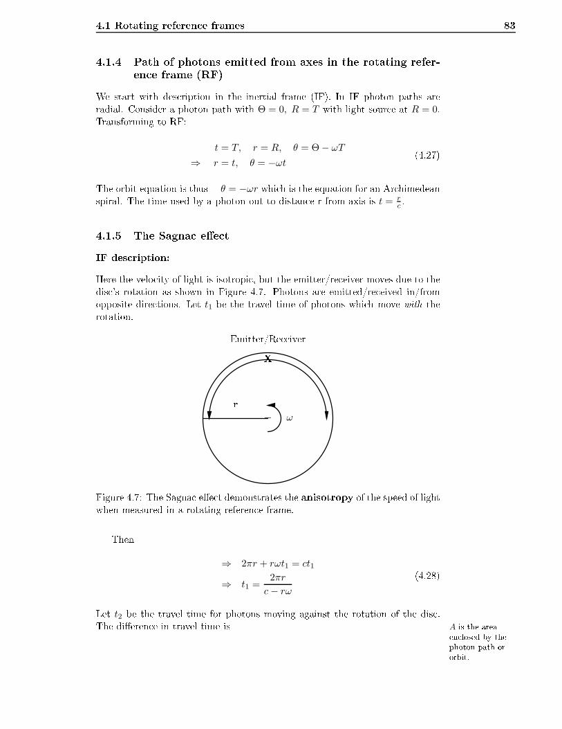
4.1 Rotating referen e frames 834.1.4 Path of photons emitted from axes in the rotating refer-en e frame (RF)We start with des ription in the inertial frame (IF). In IF photon paths areradial. Consider a photon path with Θ = 0, R = T with light sour e at R = 0.Transforming to RF:t = T, r = R, θ = Θ − ωT

⇒ r = t, θ = −ωt(4.27)The orbit equation is thus θ = −ωr whi h is the equation for an Ar himedeanspiral. The time used by a photon out to distan e r from axis is t = r

c .4.1.5 The Sagna ee tIF des ription:Here the velo ity of light is isotropi , but the emitter/re eiver moves due to thedis 's rotation as shown in Figure 4.7. Photons are emitted/re eived in/fromopposite dire tions. Let t1 be the travel time of photons whi h move with therotation.+r

ω

XEmitter/Re eiver

Figure 4.7: The Sagna ee t demonstrates the anisotropy of the speed of lightwhen measured in a rotating referen e frame.Then⇒ 2πr + rωt1 = ct1

⇒ t1 =2πr

c− rω

(4.28)Let t2 be the travel time for photons moving against the rotation of the dis .The dieren e in travel time is A is the areaen losed by thephoton path ororbit.

84 Chapter 4. A elerated Referen e Frames∆t = t1 − t2 = 2πr

(1

c− rω− 1

c+ rω

)

=2πr2rω

c2 − r2ω2

= γ2 4Aω

c2

(4.29)RF des ription:

ds2= 0 along theworld line of aphoton ds2 = −

(1 − r2ω2

c2

)c2dt2 + r2dθ2 + 2r2ωdθdtlet θ =

dθ

dt

r2θ2 + 2r2ωθ − (c2 − r2ω2) = 0

θ =−r2ω ±

√(r4ω2 + r2c2 − r4ω2)

r2

θ = −ω ± rc

r2

= −ω ± c

r

(4.30)The speed of light: v± = rθ = −rω ± c. We see that in the rotating frame RF,the measured ( oordinate) velo ity of light is NOT isotropi . The dieren e inthe travel time of the two beams is∆t =

2πr

c− rω− 2πr

c+ rω

= γ2 4Aω

c2

(4.31)The oordinate lo ks are not Einstein syn hronized in RF, but they representa globally well dened time. As measured with lo ally Einstein syn hronized lo ks the velo ity of light is isotropi . But as shown, it is not possible toEinstein syn hronize lo ks around a losed urve in RF. (See Phil. Mag. series6, vol. 8 (1904) for Mi helson's arti le)4.2 Hyperboli ally a elerated referen e framesConsider a parti le moving along a straight line with velo ity u and a elerationa = du

dT . Rest a eleration is a.⇒ a =

(1 − u2/c2

)3/2a. (4.32)Assume that the parti le has onstant rest a eleration a = g. That is

du

dT=(1 − u2/c2

)3/2g. (4.33)

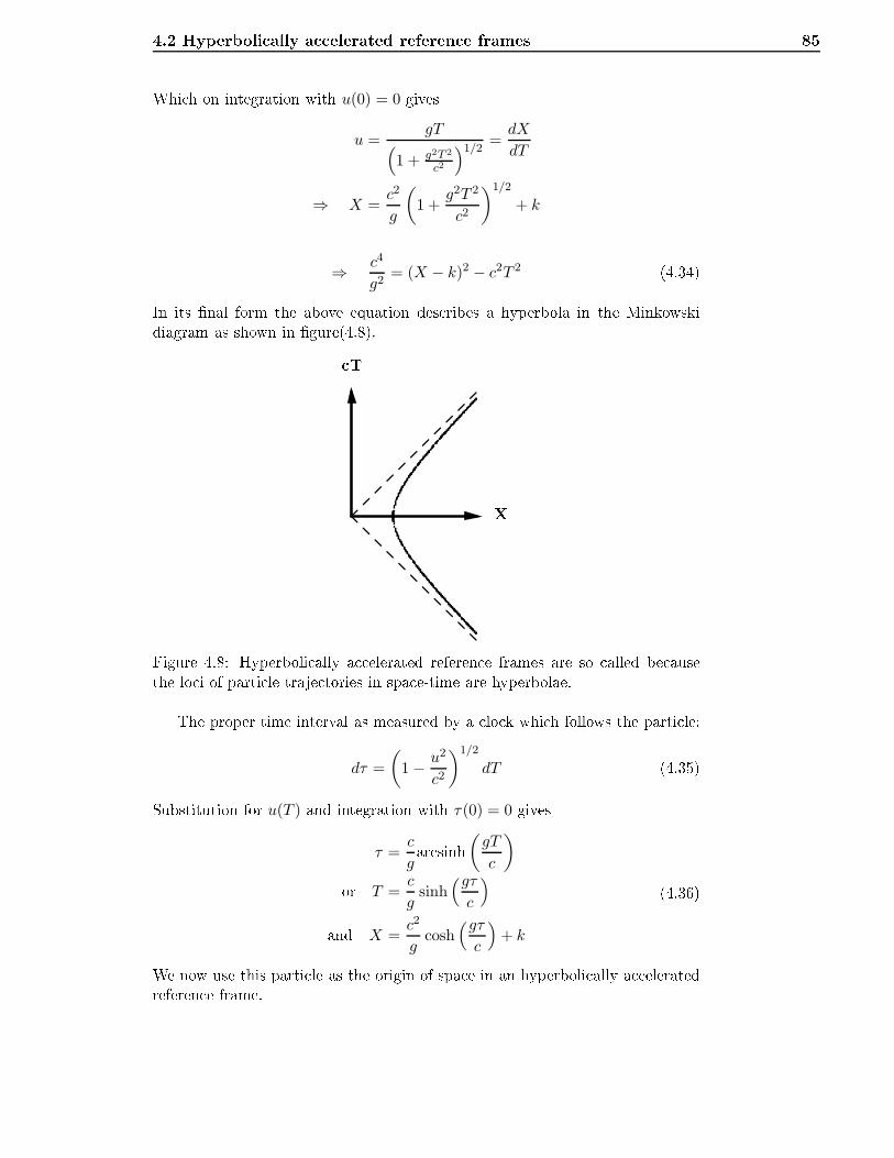
4.2 Hyperboli ally a elerated referen e frames 85Whi h on integration with u(0) = 0 givesu =

gT(1 + g2T 2

c2

)1/2=dX

dT

⇒ X =c2

g

(1 +

g2T 2

c2

)1/2

+ k

⇒ c4

g2= (X − k)2 − c2T 2 (4.34)In its nal form the above equation des ribes a hyperbola in the Minkowskidiagram as shown in gure(4.8). T

XFigure 4.8: Hyperboli ally a elerated referen e frames are so alled be ausethe lo i of parti le traje tories in spa e-time are hyperbolae.The proper time interval as measured by a lo k whi h follows the parti le:

dτ =

(1 − u2

c2

)1/2

dT (4.35)Substitution for u(T ) and integration with τ(0) = 0 givesτ =

c

gar sinh(gT

c

)or T =c

gsinh

(gτc

)and X =c2

gcosh

(gτc

)+ k

(4.36)We now use this parti le as the origin of spa e in an hyperboli ally a eleratedreferen e frame.

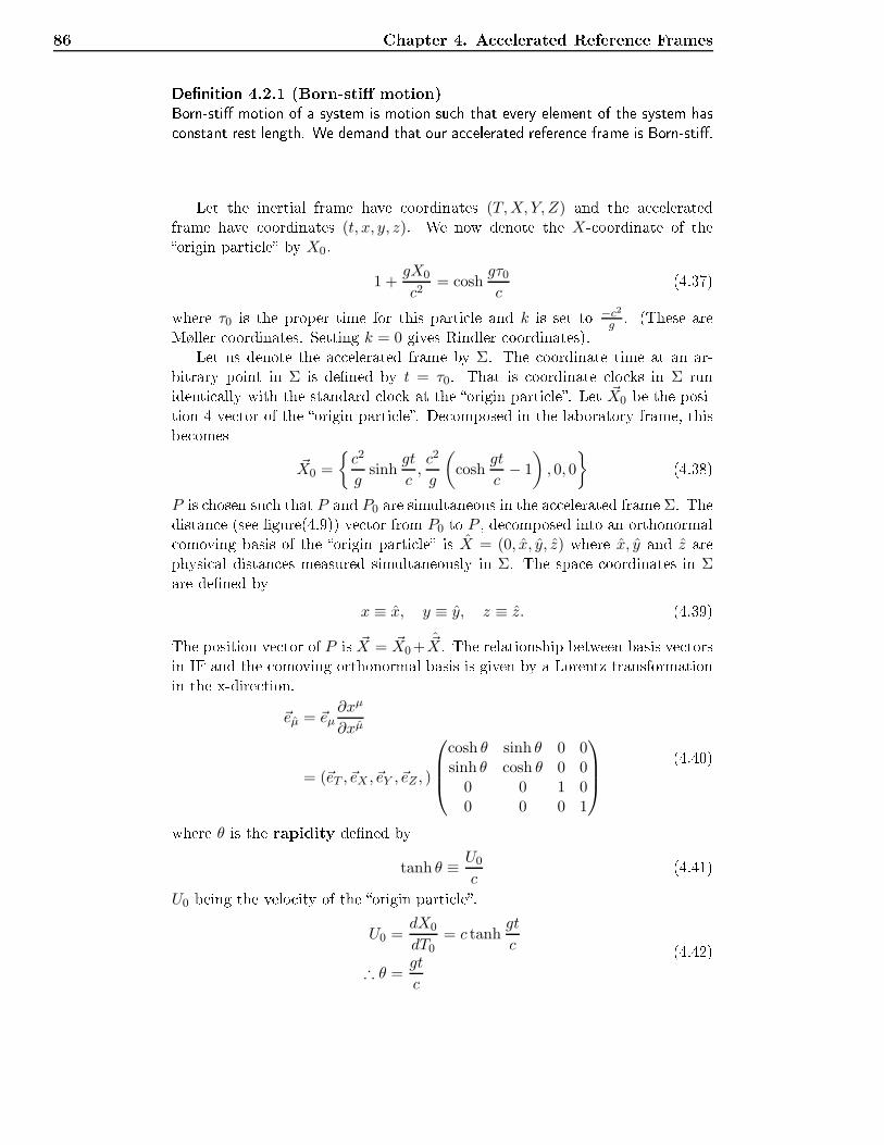
86 Chapter 4. A elerated Referen e FramesDenition 4.2.1 (Born-sti motion)Born-sti motion of a system is motion su h that every element of the system has onstant rest length. We demand that our a elerated referen e frame is Born-sti.Let the inertial frame have oordinates (T,X, Y, Z) and the a eleratedframe have oordinates (t, x, y, z). We now denote the X- oordinate of theorigin parti le by X0.1 +

gX0

c2= cosh

gτ0c

(4.37)where τ0 is the proper time for this parti le and k is set to −c2g . (These areMøller oordinates. Setting k = 0 gives Rindler oordinates).Let us denote the a elerated frame by Σ. The oordinate time at an ar-bitrary point in Σ is dened by t = τ0. That is oordinate lo ks in Σ runidenti ally with the standard lo k at the origin parti le. Let ~X0 be the posi-tion 4-ve tor of the origin parti le. De omposed in the laboratory frame, thisbe omes

~X0 =

c2

gsinh

gt

c,c2

g

(cosh

gt

c− 1

), 0, 0

(4.38)P is hosen su h that P and P0 are simultaneous in the a elerated frame Σ. Thedistan e (see gure(4.9)) ve tor from P0 to P , de omposed into an orthonormal omoving basis of the origin parti le is X = (0, x, y, z) where x, y and z arephysi al distan es measured simultaneously in Σ. The spa e oordinates in Σare dened by

x ≡ x, y ≡ y, z ≡ z. (4.39)The position ve tor of P is ~X = ~X0+ ~X. The relationship between basis ve torsin IF and the omoving orthonormal basis is given by a Lorentz transformationin the x-dire tion.~eµ = ~eµ

∂xµ

∂xµ

= (~eT , ~eX , ~eY , ~eZ , )

cosh θ sinh θ 0 0sinh θ cosh θ 0 0

0 0 1 00 0 0 1

(4.40)where θ is the rapidity dened by

tanh θ ≡ U0

c(4.41)

U0 being the velo ity of the origin parti le.U0 =

dX0

dT0= c tanh

gt

c

∴ θ =gt

c

(4.42)

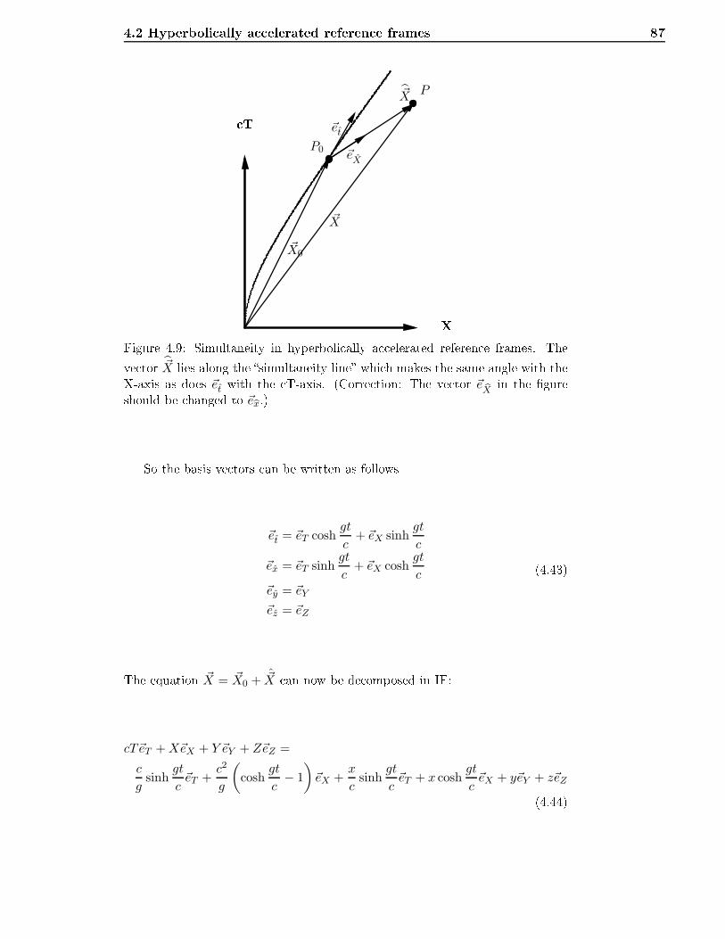
4.2 Hyperboli ally a elerated referen e frames 87 T

X~X0

P0

~et

P

~eX

~X

~X

Figure 4.9: Simultaneity in hyperboli ally a elerated referen e frames. Theve tor ~X lies along the simultaneity line whi h makes the same angle with theX-axis as does ~et with the T-axis. (Corre tion: The ve tor ~e bX in the gureshould be hanged to ~ebx.)So the basis ve tors an be written as follows~et = ~eT cosh

gt

c+ ~eX sinh

gt

c

~ex = ~eT sinhgt

c+ ~eX cosh

gt

c~ey = ~eY

~ez = ~eZ

(4.43)The equation ~X = ~X0 + ~X an now be de omposed in IF:cT~eT +X~eX + Y ~eY + Z~eZ =

c

gsinh

gt

c~eT +

c2

g

(cosh

gt

c− 1

)~eX +

x

csinh

gt

c~eT + x cosh

gt

c~eX + y~eY + z~eZ(4.44)

88 Chapter 4. A elerated Referen e FramesThis then, gives the oordinate transformationsT =

c

gsinh

gt

c+x

csinh

gt

c

X =c2

g

(cosh

gt

c− 1

)+ x cosh

gt

c

Y = y

Z = z

⇒ gT

c=(1 +

gx

c2

)sinh

gt

c

1 +gX

c2=(1 +

gx

c2

)cosh

gt

cNow dividing the last two of the above equations we getgT

c=

(1 +

gX

c2

)tanh

gt

c(4.45)showing that the oordinate urves t = onstant are straight lines in the T,X-frame passing through the point T = 0, X = − c2

g . Using the identity cosh2 θ −sinh2 θ = 1 we get

(1 +

gX

c2

)2

−(gT

c

)2

=(1 +

gx

c2

)2 (4.46)showing that the oordinate urves x = onstant are hypebolae in the T,X-diagram.The line element (the metri ) gives :ds2 is aninvariantquantity ds2 = −c2dT 2 + dX2 + dY 2 + dZ2

= −(1 +gx

c2)2c2dt2 + dx2 + dy2 + dz2 (4.47)Note: When the metri is diagonal the unit ve tors are orthogonal.Clo ks at rest in the a elerated system:

dx = dy = dz = 0, ds2 = −c2dτ2

⇓

−c2dτ2 = −(1 +gx

c2)2c2dt2

⇓

dτ = (1 +gx

c2)dt (4.48)Here dτ is the proper time and dt the oordinate time.An observer in the a elerated system Σ experien es a gravitational eld inthe negative x-dire tion. When x < 0 then dτ < dt. The oordinate lo ks

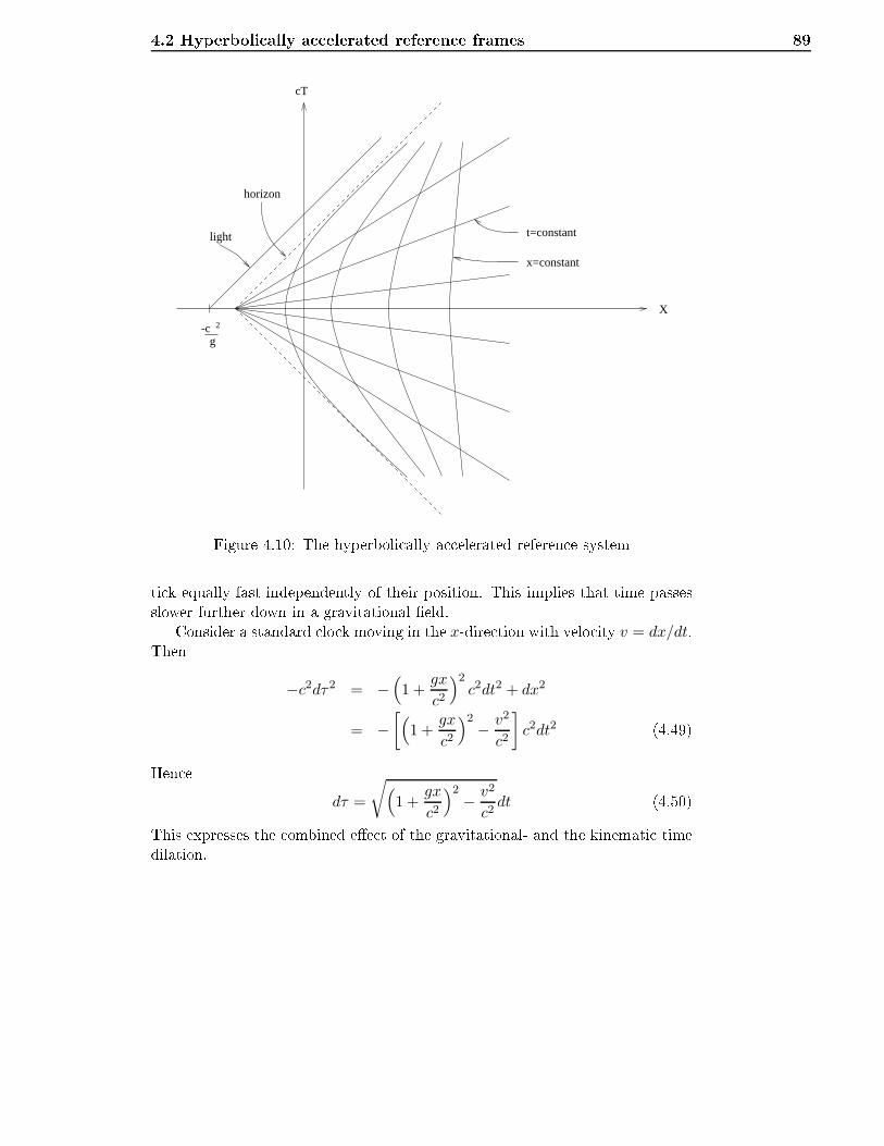
4.2 Hyperboli ally a elerated referen e frames 89

X

cT

light t=constant

x=constant

g-c 2

horizon

Figure 4.10: The hyperboli ally a elerated referen e systemti k equally fast independently of their position. This implies that time passesslower further down in a gravitational eld.Consider a standard lo k moving in the x-dire tion with velo ity v = dx/dt.Then−c2dτ2 = −

(1 +

gx

c2

)2c2dt2 + dx2

= −[(

1 +gx

c2

)2− v2

c2

]c2dt2 (4.49)Hen e

dτ =

√(1 +

gx

c2

)2− v2

c2dt (4.50)This expresses the ombined ee t of the gravitational- and the kinemati timedilation.

90 Chapter 4. A elerated Referen e FramesProblems4.1. Relativisti rotating dis A dis rotates with onstant angular velo ity in ω in its own plane andaround a xed axis A. The axis is hosen to be the origin in a non-rotatingCartesian oordinate system (x, y). (The z- oordinate will be negle tedfrom now on.) The motion of a given point on the dis an be expressedasx = r cos(ωt + φ) (4.51)y = r sin(ωt + φ) (4.52)where (r, φ) are oordinates spe ifying the point at the dis .(a) An observer is able to move on the dis and performs measurements ofdistan e between neighboring points at dierent lo ations on the dis . Themesurements are performed when the observer is stationary with respe tto the dis . The result is assumed to be the same as that measured in aninertial frame with the same velo ity as the observer at the time of themeasurement. The lengths measured by the observer are given by

dℓ2 = f1(r, φ)dr2 + f2(r, φ)dφ2 (4.53)Find f1(r, φ) og f2(r, φ).We now assume that the observer measures the distan e from the axis A toa point (R, 0) along the line φ = 0, by adding the result of measurementsbetween neighboring points. What is the result the observer nds?Furthermore the observer measures the distan e around the ir le r = R.What is then found? In what way, based on this result, is it possible todedu e that the metri onsidered by the observer is non-Eu lidean? Willthe observer nd a negative or positive urvature of the dis ?(b) We introdu e the oordinates (x, y) that follow the rotating dis . They aregiven byx = r cosφ, (4.54)y = r sinφ (4.55)Find the invariant interval ds2 = dx2+dy2−dt2 in terms of the oordinates

(x, y, t).Write down the relativisti Lagrangian of a free parti le and ndthe equation of motion (EOM) expressed in the same oordinates. Showthat the equations enter a non-relativisti , with a Coriolis term and aCentrifugal term, when we assume that ωr ≪ 1 and that the velo ity ofthe parti le satises v ≪ 1.( ) Light signals are sent from the axis A. How will the paths of the light beas seen from the (x, y)-system? Draw a gur that illustrates this. A lightsignal with the fequen y ν0 is re eived by the observer in r = R, φ = 0.Whi h frequen y ν will be measured by the observer vil han måle?

Problems 91(d) We now assume that lo ks are tightly pa ked around the dis r = R.The lo ks are non-moving with respe t to the dis , and are standard lo ks, measuring proper time of the lo k. We now want to syn hronizethe lo ks and start out with a lo k at the point (R, 0).The lo ks arethen syn hronized in the dire tion of in reasing φ in the following way:When the lo k is tuned at the point φ, the lo k at the neighboring pointφ + dφ is also tuned so that they show the same time at simultaneity inthe instantaneous rest frame of the two lo ks.Show that there is a problem with syn hronization when this pro ess isperformed around the entire ir le, by the fa t that the lo k we startedout with is no longer syn hronous with the neighboring lo k whi h is tueda ording to the syn hronization pro ess. Find the time dieren e betweenthese two lo ks.(e) Lokally around a point (r, φ, t) we an dene an inertial system being aninstantaneous rest frame of the point (r, φ) on the dis . We introdu e anorthonormal set of basis ve tors ~eλ, ~eη and ~eξ in this frame. The ve tor~eλ points along the time axis of the system, ~eξ points radially, and eηtangentially. Find the ve tors expressed by ~et, ~ex and ~ey.The path of a light signal from A is studied at the lo al inertial framesalong the path. Find how the spatial dire tion of the light signal hangesrelative to the basis ve tors ~eξ and ~eη (outwards) along the paths. Is thisresult in a ordan e with what was earlier found on the path of the lightin the (x, y)-system?4.2. Free parti le in a hyperboli referen e frameThe metri for a two-dimensional spa e is given by

ds2 = −V 2dU2 + dV 2. (4.56)(a) Find the Euler-Lagrange equations for the motion of a free parti le usingthis metri . Show that they admit the following solutions:1

V=

1

V0cosh(U − U0).What is the physi al interpretation of the onstants V0 and U0?(b) Show that these are straight lines in the oordinate system (t, x) given by

x = V coshU

t = V sinhU. (4.57)Express the speed of the parti le in terms of U0, and its x- omponent att = 0 in terms of V0 and U0. Find the interval ds2 expressed in termsof x and t and show that the spa e in whi h the parti le is moving, is aMinkowski spa e with one time and one spatial dimension.

92 Chapter 4. A elerated Referen e Frames( ) Express the ovariant omponent pU of the momentum using pt = −E andpx = p, and show that it is a onstant of motion. How an this fa t bedire tly extra ted from the metri ? Show further that the ontravariant omponent pU is not a onstant of motion. Are pV or pV onstants ofmotion?4.3. Uniformly a elerated system of referen eWe will now study a urved oordinate system (U, V ) in a two-dimensionalMinkowski-spa e. The onne tion with the Carthesian system (t, x) is given by

t = V sinh(aU), (4.58)x = V cosh(aU), (4.59)where a is a onstant. (See ex . 5.1.)(a) Draw the oordinate lines U and V in a (t, x)-diagram. Cal ulate the basisve tors ~eU and ~eV and draw them at some hosen points in the diagram.Find the metri ds2 = dx2 − dt2 expressed by U and V .(b) We now assume that a parti le has a path in spa etime so that it followsone of the urves V = onstant. Su h a motion is alled hyperboli motion.Why ?Show that the parti le has onstant a eleration g along the path when thea eleration is measured in the instantaneous rest frame of teh parti le.Find the a eleration. Find also the the velo ity and a elereation of theparti le in the stationary system (t, x).( ) Show that at any point on the parti le traje tory, the dire tion of the

(U, V )- oordinate axis will overlap with the time and spatial axis of theinstantaneous rest frame of the parti le. Explain why it is possible to seefrom the line element that the V - oordinate measures length along thespatial axis, whereas the U - oordinate, whi h is the oordinate time, is ingeneral not the proper time of the parti le? For what value of V is the oordinate equal to the proper time?The (U, V )- oordinate system an be onsidered as an attempt to on-stru t, from the instantaneous rest frames along the path, a oordinatesystem overing the entire spa etime. Explain why this is not possiblefor the entire spa e. (Hint: There is a oordinate singularity at a ertaindistan e from the traje tory of the parti le).(d) A rod is moving in the dire tion af its own length. At the time t = 0the rod is at rest, but still a elerated. The length of the rod measuredin the stationary system is L at this time. The rod moves so that theforwars point of the rod has onstant rest a eleration measured in theinstantaneous rest frame.We assume that the a eleration of the rod nds pla e so that the innites-imal distan e dℓ between neighboring points on the rod, measured in theinstantaneous rest frame are onstant. Find the motion of the rear point of

Problems 93the rod in the stationary referen e system. Why is there a maximal lengthof the rod, Lmax?If the rear point of the rod has onstant a eleration, and the rod is a - elerated as previously in this ex er ise, then is there a maximal value ofL?(e) A spa eship leaves the Earth at the time t = 0 and moves with a onstanta eleration g, equal to the gravitational onstant at the Earth, into spa e.Find how far the ship has travelled during 10 years of proper time of theship.Radiosignals are sent from the Earth towards the spa eship. Show thatsignals that are sent after a given time T will never rea h teh ship (even ifthe signals travel with the speed of light). Find T . At what time are thesignals sent from the Earth if they rea h the ship after 10 years (propertime of the ship)?Cal ulate the frequen y of the radio signals re eived by the ship, given bythe frequen y ν0 (emitter frequen y) and the time t0 (emitter time). In-vestigate the behaviour of the frequen y when t0 → T .4.4. The proje tion tensorLet the metri tensor of the spa etime in a oordinate system K have ompo-nents gµν . An observer has a 4-velo ity given by ~u.An arbitrary ve tor ~a an be de omposed into a omponent ~a‖ parallel to ~u anda omponent ~a⊥ orthogonal to ~u, so that ~a = ~a‖ + ~a⊥.(a) Show that:

~a‖ = (~a · ~u)~u/u2 = −(~a · ~u)~u, (4.60)~a⊥ = ~a+ (~a · ~u)~u (4.61)Equation (4.61) an be rewritten by the proje tion tensor

P = I + ~u⊗ u (4.62)where I is the ve torial 1-form, that an be written asI = δµ ν~eµ ⊗ ων (4.63)and u has omponents uµ = gµνu

ν .Show that (4.61) an be written as~a⊥ = P ( ,~a) (4.64)so that the omponents of ~a⊥ and ~a are related viaaµ⊥ = Pµνa

ν (4.65)Sin e ~u is tangent ve tor of the world line of the observer, then Pµνaν isthe proje tion of ~a in the spatial plane of simultaneityorthogonal to thetime ve tor in the lo al orthonormal basis of the observer.

94 Chapter 4. A elerated Referen e Frames(b) Assume that the observer is non-moving in K. Find the mixed and ovari-ant omponents of P .( ) Let ~a be the 4-a eleration of a parti le. Whart kind of motion does the o-variant equation Pµν daν

dτ = 0 des ribe. Explain! (Hint: Find the time andspa e omponents of this equation. In an instantaneous rest frame of theparti le, d~a/dτ = (g2, d~g/dτ) where the 3-ve tor ~g is the rest a eleration).(d) Consider an interval dxµ in spa etime. It has a omponent orthogonal to a4-velo ity ~u given by dσµ = Pµαdxα. The invariant spatial line element dℓis given by dℓ2 = dσµdσµ, and the omponents of the spatial metri tensor,i.e. the metri tensor in the spatial plane orthogonal to ~u, is dened by

dℓ2 = γµνdxµdxν . Find γµν given by gµν and uα.Find in parti ular γij when ~u is the 4-velo ity of an observer at rest in K.

Chapter 5Covariant Dierentiation5.1 Dierentiation of formsWe must have a method of dierentiation that maintains the anti symmetry,thus making sure that what we end up with after dierentiation is still a form.5.1.1 Exterior dierentiationThe exterior derivative of a 0-form, i.e. a s alar fun tion, f , is given by:df =

∂f

∂xµωµ = f,µω

µ (5.1)where ωµ are oordinate basis forms:ωµ(

∂

∂xν) = δµν (5.2)We then (in general) get:

ωµ = δµνων =

∂xµ

∂xνων = dxµ (5.3)In oordinate basis we an always write the basis forms as exterior derivativesof the oordinates. The dierential dxµ is given by

dxµ(d~r) = dxµ (5.4)where d~r is an innitesimal position ve tor. dxµ are not innitesimal quantities.In oordinate basis the exterior derivative of a p-formα =

1

p!αµ1···µpdx

µ1 ∧ · · · ∧ dxµp (5.5)will have the following omponent form:d α =

1

p!αµ1···µp,µ0dx

µ0 ∧ dxµ1 ∧ · · · ∧ dxµp (5.6)95

96 Chapter 5. Covariant Dierentiationwhere , µ0 ≡ ∂∂xµ0 . The exterior derivative of a p-form is a (p+ 1)-form.Consider the exterior derivative of a p-form α.

dα =1

p!αµ1···µp,µ0dx

µ0 ∧ · · · ∧ dxµp . (5.7)Let (dα)µ0···µp be the form omponents of dα. They must, by denition, beantisymmetri under an arbitrary inter hange of indi es.dα =

1

(p+ 1)!(dα)µ0···µpdx

µ0 ∧ · · · ∧ dxµpwhi h, by (5.7) ⇒ =1

p!α[αµ1···µp,µ0 ]dx

µ0 ∧ · · · ∧ dxµp

∴ (dα)µ0···µp = (p + 1)α[µ1···µp,µ0] (5.8)The form equation dα = 0 in omponent form isα[µ1···µp,µ0] = 0 (5.9)Example 5.1.1 (Outer produ t of 1-forms in 3-spa e)

α = αidxi xi = (x, y, z)

dα = αi,jdxj ∧ dxi

(5.10)Also, assume that dα = 0. The orresponding omponent equation isα[i,j] = 0 ⇒ αi,j − αj,i = 0

⇒ ∂αx∂y

− ∂αy∂x

= 0,∂αx∂z

− ∂αz∂x

= 0,∂αy∂z

− ∂αz∂y

= 0(5.11)whi h orresponds to

∇×~α = 0 (5.12)The outer produ t of an outer produ t!d2α ≡ d(dα)

d2α =1

p!αµ1···µp,ν1ν2dx

ν2 ∧ dxν1 ∧ · · · ∧ dxµp(5.13)

,ν1ν2 ≡ ∂2

∂xν1∂xν2(5.14)

5.1 Dierentiation of forms 97Sin e,ν1ν2 ≡ ∂2

∂xν1∂xν2=,ν2ν1≡

∂2

∂xν2∂xν1(5.15)summation over ν1 and ν2 whi h are symmetri in αµ1···µp,ν1ν2 and antisymmetri in the basis we get Poin aré's lemma (valid only for s alar elds)

d2α = 0 (5.16)This orresponds to the ve tor equation∇ · (∇× ~A) = 0 (5.17)Let α be a p-form and β be a q-form. Then

d(α ∧ β) = dα ∧ β + (−1)pα ∧ dβ (5.18)5.1.2 Covariant derivativeThe general theory of relativity ontains a ovarian e prin iple whi h statesthat all equations expressing laws of nature must have the same form irrespe tiveof the oordinate system in whi h they are derived. This is a hieved by writingall equations in terms of tensors. Let us see if the partial derivative of ve tor omponents transform as tensor omponents. Given a ve tor ~A = Aµ~eµ =Aµ

′

~eµ′ with the transformation of basis given by∂

∂xν′=∂xν

∂xν′∂

∂xν(5.19)So that

Aµ′

,ν′ ≡ ∂

∂xν′

(Aµ

′

)

=∂xν

∂xν′∂

∂xν

(Aµ

′

)

=∂xν

∂xν′∂

∂xν

(∂xµ′

∂xµAµ)

=∂xν

∂xν′∂xµ′

∂xµAµ,ν +

∂xν

∂xν′Aµ

∂2xµ′

∂xν∂xµ(5.20)The rst term orresponds to a tensorial transformation. The existen e of thelast term shows that Aµ,ν does not, in general, transform as the omponents ofa tensor. Note that Aµ,ν will transform as a tensor under linear transformationssu h as the Lorentz transformations.The partial derivative must be generalized su h as to ensure that when it isapplied to tensor omponents it produ es tensor omponents.

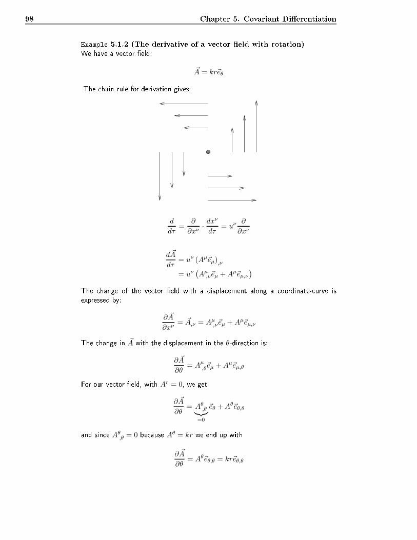
98 Chapter 5. Covariant DierentiationExample 5.1.2 (The derivative of a ve tor eld with rotation)We have a ve tor eld:~A = kr~eθThe hain rule for derivation gives:

d

dτ=

∂

∂xν· dx

ν

dτ= uν

∂

∂xν

d ~A

dτ= uν (Aµ~eµ),ν

= uν(Aµ,ν~eµ +Aµ~eµ,ν

)The hange of the ve tor eld with a displa ement along a oordinate- urve isexpressed by:∂ ~A

∂xν= ~A,ν = Aµ,ν~eµ +Aµ~eµ,νThe hange in ~A with the displa ement in the θ-dire tion is:∂ ~A

∂θ= Aµ,θ~eµ +Aµ~eµ,θFor our ve tor eld, with Ar = 0, we get

∂ ~A

∂θ= Aθ,θ︸︷︷︸

=0

~eθ +Aθ~eθ,θand sin e Aθ,θ = 0 be ause Aθ = kr we end up with∂ ~A

∂θ= Aθ~eθ,θ = kr~eθ,θ

5.2 The Christoel Symbols 99We now need to al ulate the derivative of ~eθ. We have:x = r cos θ y = r sin θUsing ~eµ = ∂

∂xµ we an write:~eθ =

∂

∂θ=∂x

∂θ

∂

∂x+∂y

∂θ

∂

∂y

= −r sin θ~ex + r cos θ~ey

~er =∂

∂r= cos θ~ex + sin θ~eyGives:

~eθ,θ = −r cos θ~ex − r sin θ~ey

= −r(cos θ~ex + sin θ~ey) = −r~erThis gives us nally:∂ ~A

∂θ= −kr2~erThus ∂ ~A

∂θ 6= 0 even if ~A = Aθ~eθ and Aθ,θ = 0.5.2 The Christoel SymbolsThe ovariant derivative was introdu ed by Christoel to be able to dierenti-ate tensor elds. It is dened in oordinate basis by generalizing the partiallyderivative Aµ,ν to a derivative written as Aµ;ν and whi h transforms tensorially,Aµ

′

;ν′ ≡∂xµ

′

∂xµ· ∂x

ν

∂xν′Aµ;ν . (5.21)The ovariant derivative of the ontravariant ve tor omponents are written as:

Aµ;ν ≡ Aµ,ν +AαΓµαν (5.22)This equation denes the Christoel symbols Γµαν , whi h are also alled the onne tion oe ients in oordinate basis. From the transformation formulaefor the two rst terms follows that the Christoel symbols transform as:Γα

′

µ′ν′ =∂xν

∂xν′∂xµ

∂xµ′∂xα

′

∂xαΓαµν +

∂xα′

∂xα∂2xα

∂xµ′∂xν′(5.23)The Christoel symbols do not transform as tensor omponents. It is possible to an el all Christoel symbols by transforming into a lo ally Cartesian oordinate

100 Chapter 5. Covariant Dierentiationsystem whi h is o-moving in a lo ally non-rotating referen e frame in free fall.Su h oordinates are known as Gaussian oordinates.In general relativity theory an inertial frame is dened as a non-rotatingframe in free fall. The Christoel symbols are 0 (zero) in a lo ally Cartesian oordinate system whi h is o-moving in a lo al inertial frame. Lo al Gaussian oordinates are indi ated with a bar over the indi es, givingΓαµν = 0 (5.24)A transformation from lo al Gaussian oordinates to any oordinates leads to:

Γα′

µ′ν′ =∂xα

′

∂xα∂2xα

∂xµ′∂xν′(5.25)This equation shows that the Christoel symbols are symmetri in the two lowerindi es, ie.

Γα′

µ′ν′ = Γα′

ν′µ′ (5.26)Example 5.2.1 (The Christoel symbols in plane polar oordinates)x = r cos θ, y = r sin θ

r =√x2 + y2, θ = arctan

y

x

∂x

∂r= cos θ,

∂x

∂θ= −r sin θ

∂r

∂x=x

r= cos θ,

∂r

∂y= sin θ

∂y

∂r= sin θ,

∂y

∂θ= r cos θ

∂θ

∂x= −sin θ

r,

∂θ

∂y=

cos θ

r

Γrθθ =∂r

∂x

∂2x

∂θ2+∂r

∂y

∂2y

∂θ2

= cos θ(−r cos θ) + sin θ(−r sin θ)

= −r(cos θ2 + sin θ2) = −r

Γθrθ = Γθθr =∂θ

∂x

∂2x

∂θ∂r+∂θ

∂y

∂2y

∂θ∂r

= −sin θ

r(− sin θ) +

cos θ

r(cos θ)

=1

r

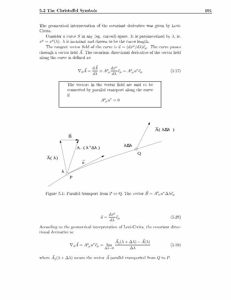
5.2 The Christoel Symbols 101The geometri al interpretation of the ovariant derivative was given by Levi-Civita.Consider a urve S in any (eg. urved) spa e. It is parameterized by λ, ie.xµ = xµ(λ). λ is invariant and hosen to be the urve length.The tangent ve tor eld of the urve is ~u = (dxµ/dλ)~eµ. The urve passesthrough a ve tor eld ~A. The ovariant dire tional derivative of the ve tor eldalong the urve is dened as:

∇~u~A =

d ~A

dλ≡ Aµ;ν

dxν

dλ~eµ = Aµ;νu

ν~eµ (5.27)The ve tors in the ve tor eld are said to be onne ted by parallel transport along the urveifAµ;νu

ν = 0

λ)A(

B

)∆λA +λ(

u

λ+∆λ

Q

P

A( λ+∆λ)

λFigure 5.1: Parallel transport from P to Q. The ve tor ~B = Aµ;νuν∆λ~eµ

~u =dxµ

dλ~eµ (5.28)A ording to the geometri al interpretation of Levi-Civita, the ovariant dire -tional derivative is:

∇~u~A = Aµ;νu

ν~eµ = lim∆λ→0

~A‖(λ+ ∆λ) − ~A(λ)

∆λ(5.29)where ~A‖(λ+ ∆λ) means the ve tor ~A parallel transported from Q to P .

102 Chapter 5. Covariant Dierentiation5.3 Geodesi urvesDenition 5.3.1 (Geodesi urves)A geodesi urve is dened in su h a way that,the ve tors of the tangent ve tor eldof the urve is onne ted by parallell transport.This denition says that geodesi urves are 'as straight as possible'.If ve tors in a ve tor eld ~A(λ) are onne ted by parallell transport by a dis-pla ement along a ve tor ~u , we have Aµ;νuν = 0. For geodesi urves, we thenhave:uµ;νu

ν = 0 (5.30)whi h is the geodesi equation.(uµ,ν + Γµανu

α)uν = 0 (5.31)Then we are using that ddλ ≡ dxν

dλ∂∂xν = uν ∂

∂xν :duµ

dλ= uν

∂uµ

∂xν= uνuµ,ν (5.32)The geodesi equation an also be written as:

duµ

dλ+ Γµανu

αuν = 0 (5.33)Usual notation: ˙ = ddλ

uµ =dxµ

dλ= xµ (5.34)

xµ + Γµαν xαxν = 0 (5.35)By omparing eq.5.35 with the equation of motion(5.53) for a free parti le (whi hwe dedu ed from the Lagrangian equations) , we nd the equations to be iden-ti al. Con lusion:Free parti les follow geodesi urves in spa etime.Example 5.3.1 (verti al motion of free parti le in hyperb. a . ref. frame)Inserting the Christoel symbols Γxtt = (1 + gx

c2)g from example 5.5.3 into thegeodesi equation for a verti al geodesi urve in a hyperboli ally a elerated refer-en e frame, we get:

x+ (1 +gx

c2)gt2 = 0

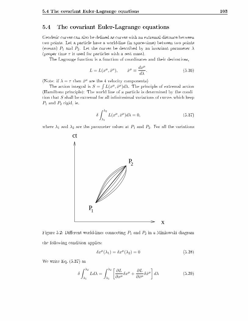
5.4 The ovariant Euler-Lagrange equations 1035.4 The ovariant Euler-Lagrange equationsGeodesi urves an also be dened as urves with an extremal distan e betweentwo points. Let a parti le have a world-line (in spa e-time) between two points(events) P1 and P2. Let the urves be des ribed by an invariant parameter λ(proper time τ is used for parti les with a rest mass).The Lagrange-fun tion is a fun tion of oordinates and their derivatives,L = L(xµ, xµ), xµ ≡ dxµ

dλ. (5.36)(Note: if λ = τ then xµ are the 4-velo ity omponents)The a tion-integral is S =

∫L(xµ, xµ)dλ. The prin iple of extremal a tion(Hamiltons-prin iple): The world-line of a parti le is determined by the ondi-tion that S shall be extremal for all innitesimal variations of urves whi h keep

P1 and P2 rigid, ie.δ

∫ λ2

λ1

L(xµ, xµ)dλ = 0, (5.37)where λ1 and λ2 are the parameter-values at P1 and P2. For all the variations

P

P

1

2

ct

xFigure 5.2: Dierent world-lines onne ting P1 and P2 in a Minkowski diagramthe following ondition applies:δxµ(λ1) = δxµ(λ2) = 0 (5.38)We write Eq. (5.37) as

δ

∫ λ2

λ1

Ldλ =

∫ λ2

λ1

[∂L

∂xµδxµ +

∂L

∂xµδxµ]dλ (5.39)

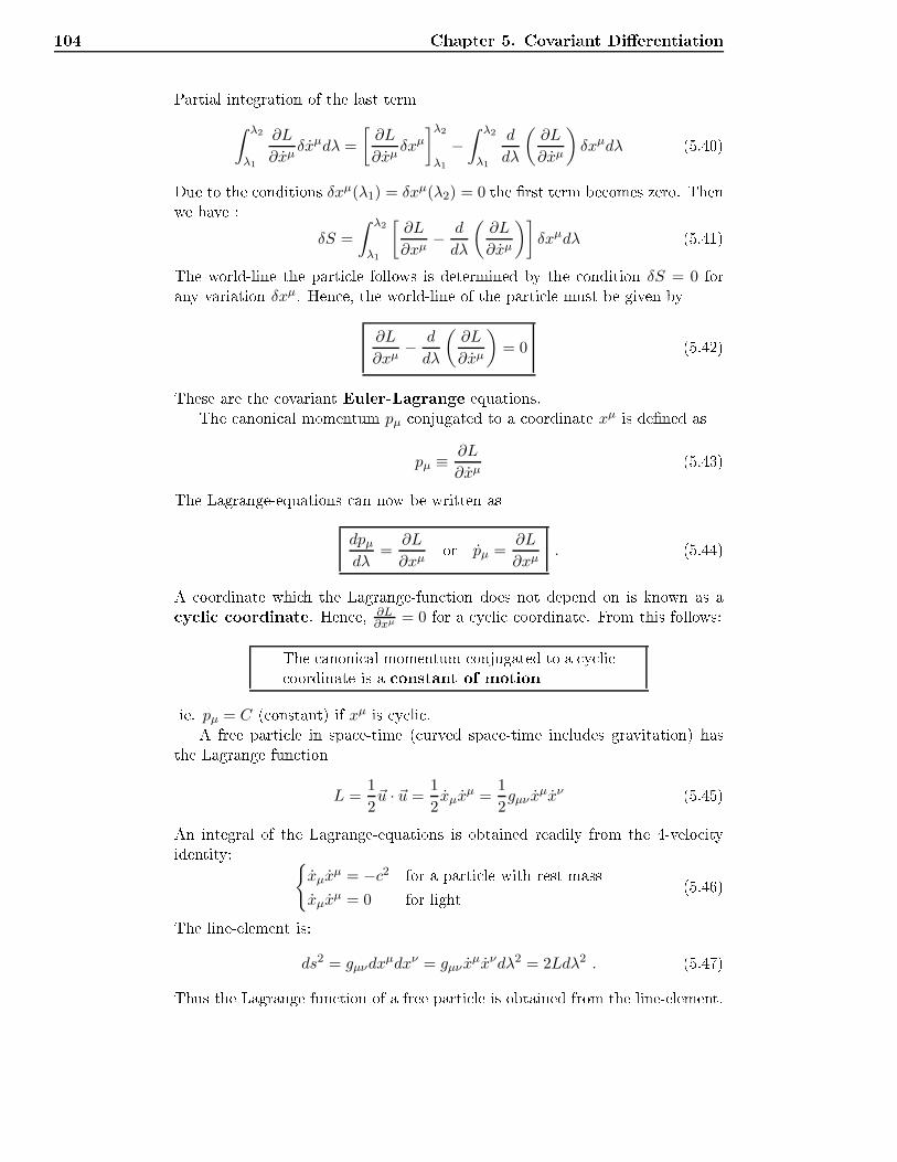
104 Chapter 5. Covariant DierentiationPartial integration of the last term∫ λ2

λ1

∂L

∂xµδxµdλ =

[∂L

∂xµδxµ]λ2

λ1

−∫ λ2

λ1

d

dλ

(∂L

∂xµ

)δxµdλ (5.40)Due to the onditions δxµ(λ1) = δxµ(λ2) = 0 the rst term be omes zero. Thenwe have :

δS =

∫ λ2

λ1

[∂L

∂xµ− d

dλ

(∂L

∂xµ

)]δxµdλ (5.41)The world-line the parti le follows is determined by the ondition δS = 0 forany variation δxµ. Hen e, the world-line of the parti le must be given by

∂L

∂xµ− d

dλ

(∂L

∂xµ

)= 0 (5.42)These are the ovariant Euler-Lagrange equations.The anoni al momentum pµ onjugated to a oordinate xµ is dened as

pµ ≡ ∂L

∂xµ(5.43)The Lagrange-equations an now be written as

dpµdλ

=∂L

∂xµor pµ =

∂L

∂xµ. (5.44)A oordinate whi h the Lagrange-fun tion does not depend on is known as a y li oordinate. Hen e, ∂L

∂xµ = 0 for a y li oordinate. From this follows:The anoni al momentum onjugated to a y li oordinate is a onstant of motionie. pµ = C ( onstant) if xµ is y li .A free parti le in spa e-time ( urved spa e-time in ludes gravitation) hasthe Lagrange fun tionL =

1

2~u · ~u =

1

2xµx

µ =1

2gµν x

µxν (5.45)An integral of the Lagrange-equations is obtained readily from the 4-velo ityidentity: xµx

µ = −c2 for a parti le with rest-massxµx

µ = 0 for light (5.46)The line-element is:ds2 = gµνdx

µdxν = gµν xµxνdλ2 = 2Ldλ2 . (5.47)Thus the Lagrange fun tion of a free parti le is obtained from the line-element.

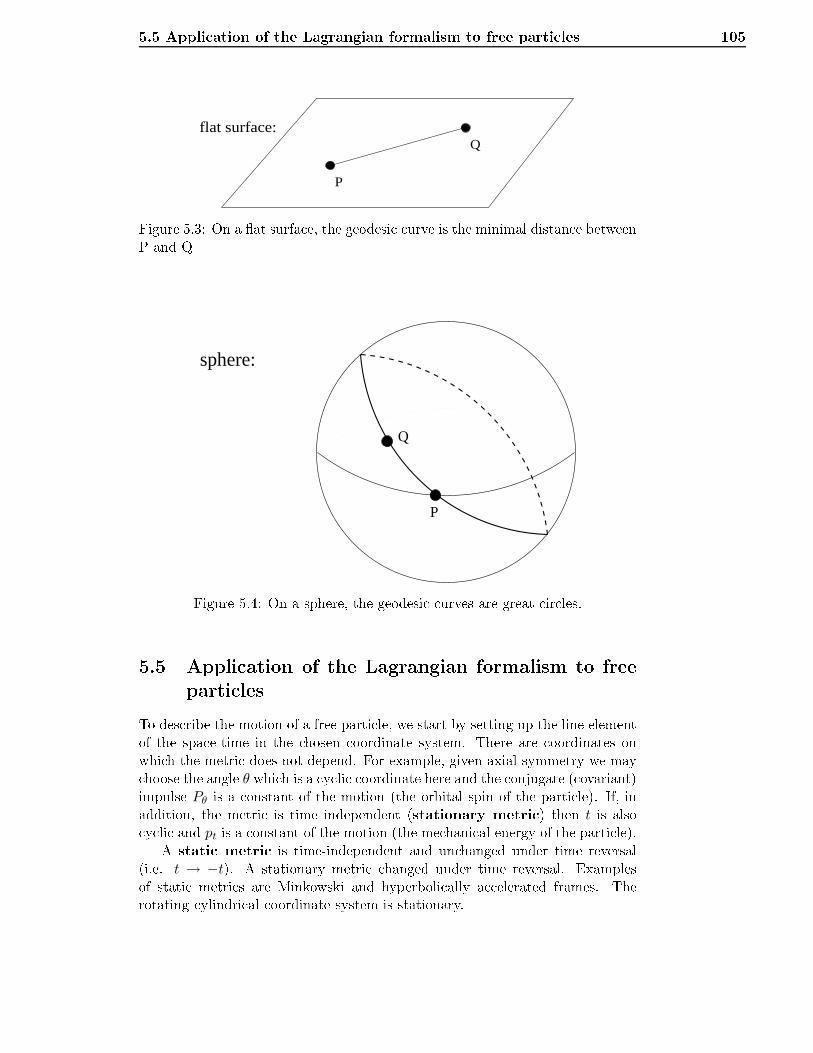
5.5 Appli ation of the Lagrangian formalism to free parti les 105flat surface:

P

Q

Figure 5.3: On a at surfa e, the geodesi urve is the minimal distan e betweenP and Qsphere:

P

Q

Figure 5.4: On a sphere, the geodesi urves are great ir les.5.5 Appli ation of the Lagrangian formalism to freeparti lesTo des ribe the motion of a free parti le, we start by setting up the line elementof the spa e-time in the hosen oordinate system. There are oordinates onwhi h the metri does not depend. For example, given axial symmetry we may hoose the angle θ whi h is a y li oordinate here and the onjugate ( ovariant)impulse Pθ is a onstant of the motion (the orbital spin of the parti le). If, inaddition, the metri is time independent (stationary metri ) then t is also y li and pt is a onstant of the motion (the me hani al energy of the parti le).A stati metri is time-independent and un hanged under time reversal(i.e. t → −t). A stationary metri hanged under time reversal. Examplesof stati metri s are Minkowski and hyperboli ally a elerated frames. Therotating ylindri al oordinate system is stationary.

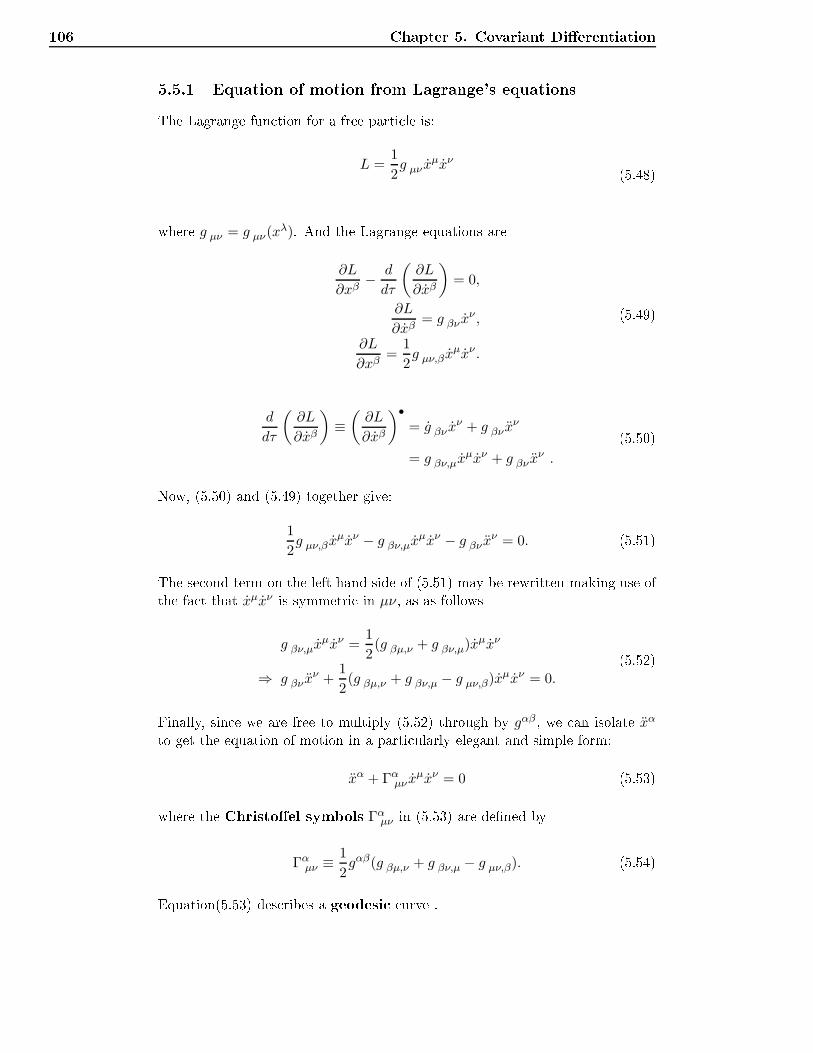
106 Chapter 5. Covariant Dierentiation5.5.1 Equation of motion from Lagrange's equationsThe Lagrange fun tion for a free parti le is:L =

1

2g µν x

µxν (5.48)where g µν = g µν(xλ). And the Lagrange equations are

∂L

∂xβ− d

dτ

(∂L

∂xβ

)= 0,

∂L

∂xβ= g βν x

ν ,

∂L

∂xβ=

1

2g µν,βx

µxν .

(5.49)d

dτ

(∂L

∂xβ

)≡(∂L

∂xβ

)•= g βν x

ν + g βν xν

= g βν,µxµxν + g βν x

ν .

(5.50)Now, (5.50) and (5.49) together give:1

2g µν,β x

µxν − g βν,µxµxν − g βν x

ν = 0. (5.51)The se ond term on the left hand side of (5.51) may be rewritten making use ofthe fa t that xµxν is symmetri in µν, as as followsg βν,µx

µxν =1

2(g βµ,ν + g βν,µ)x

µxν

⇒ g βν xν +

1

2(g βµ,ν + g βν,µ − g µν,β)x

µxν = 0.

(5.52)Finally, sin e we are free to multiply (5.52) through by gαβ , we an isolate xαto get the equation of motion in a parti ularly elegant and simple form:xα + Γαµν x

µxν = 0 (5.53)where the Christoel symbols Γαµν in (5.53) are dened byΓαµν ≡

1

2gαβ(g βµ,ν + g βν,µ − g µν,β). (5.54)Equation(5.53) des ribes a geodesi urve .

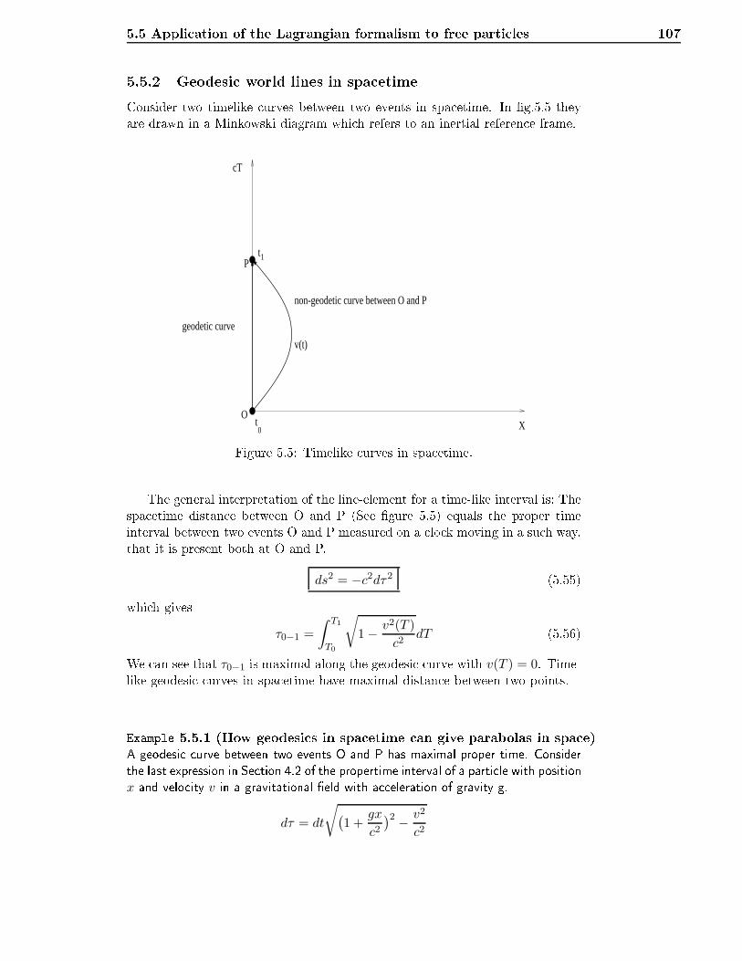
5.5 Appli ation of the Lagrangian formalism to free parti les 1075.5.2 Geodesi world lines in spa etimeConsider two timelike urves between two events in spa etime. In g.5.5 theyare drawn in a Minkowski diagram whi h refers to an inertial referen e frame.P

O

non-geodetic curve between O and P

X

geodetic curve

t

t

0

1

v(t)

cT

Figure 5.5: Timelike urves in spa etime.The general interpretation of the line-element for a time-like interval is; Thespa etime distan e between O and P (See gure 5.5) equals the proper timeinterval between two events O and P measured on a lo k moving in a su h way,that it is present both at O and P.ds2 = −c2dτ2 (5.55)whi h gives

τ0−1 =

∫ T1

T0

√1 − v2(T )

c2dT (5.56)We an see that τ0−1 is maximal along the geodesi urve with v(T ) = 0. Time-like geodesi urves in spa etime have maximal distan e between two points.Example 5.5.1 (How geodesi s in spa etime an give parabolas in spa e)A geodesi urve between two events O and P has maximal proper time. Considerthe last expression in Se tion 4.2 of the propertime interval of a parti le with position

x and velo ity v in a gravitational eld with a eleration of gravity g.dτ = dt

√(1 +

gx

c2)2 − v2

c2

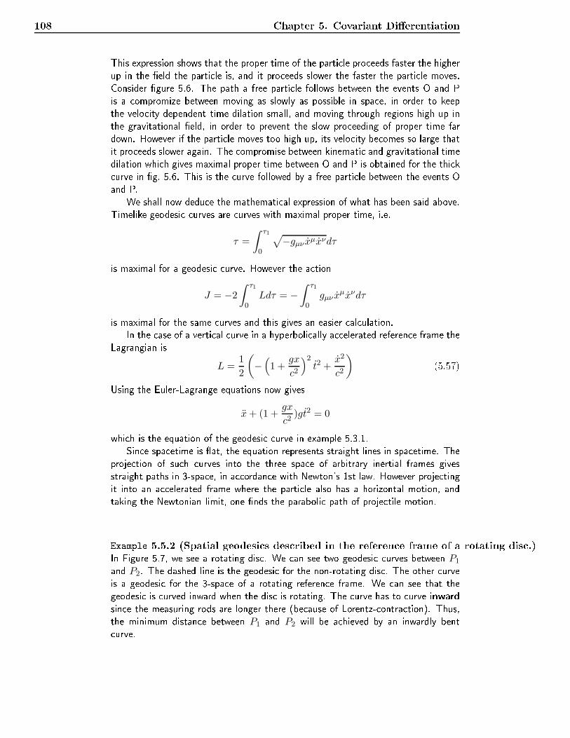
108 Chapter 5. Covariant DierentiationThis expression shows that the proper time of the parti le pro eeds faster the higherup in the eld the parti le is, and it pro eeds slower the faster the parti le moves.Consider gure 5.6. The path a free parti le follows between the events O and Pis a ompromize between moving as slowly as possible in spa e, in order to keepthe velo ity dependent time dilation small, and moving through regions high up inthe gravitational eld, in order to prevent the slow pro eeding of proper time fardown. However if the parti le moves too high up, its velo ity be omes so large thatit pro eeds slower again. The ompromise between kinemati and gravitational timedilation whi h gives maximal proper time between O and P is obtained for the thi k urve in g. 5.6. This is the urve followed by a free parti le between the events Oand P.We shall now dedu e the mathemati al expression of what has been said above.Timelike geodesi urves are urves with maximal proper time, i.e.τ =

∫ τ1

0

√−gµν xµxνdτis maximal for a geodesi urve. However the a tion

J = −2

∫ τ1

0Ldτ = −

∫ τ1

0gµν x

µxνdτis maximal for the same urves and this gives an easier al ulation.In the ase of a verti al urve in a hyperboli ally a elerated referen e frame theLagrangian isL =

1

2

(−(1 +

gx

c2

)2t2 +

x2

c2

) (5.57)Using the Euler-Lagrange equations now givesx+ (1 +

gx

c2)gt2 = 0whi h is the equation of the geodesi urve in example 5.3.1.Sin e spa etime is at, the equation represents straight lines in spa etime. Theproje tion of su h urves into the three spa e of arbitrary inertial frames givesstraight paths in 3-spa e, in a ordan e with Newton's 1st law. However proje tingit into an a elerated frame where the parti le also has a horizontal motion, andtaking the Newtonian limit, one nds the paraboli path of proje tile motion.Example 5.5.2 (Spatial geodesi s des ribed in the referen e frame of a rotating dis .)In Figure 5.7, we see a rotating dis . We an see two geodesi urves between P1and P2. The dashed line is the geodesi for the non-rotating dis . The other urveis a geodesi for the 3-spa e of a rotating referen e frame. We an see that thegeodesi is urved inward when the dis is rotating. The urve has to urve inwardsin e the measuring rods are longer there (be ause of Lorentz- ontra tion). Thus,the minimum distan e between P1 and P2 will be a hieved by an inwardly bent urve.

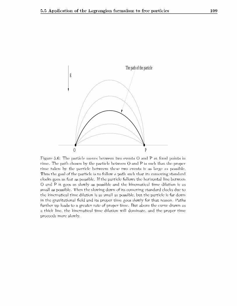
5.5 Appli ation of the Lagrangian formalism to free parti les 109The path of the particle

O P

g

Figure 5.6: The parti le moves between two events O and P at xed points intime. The path hosen by the parti le between O and P is su h that the propertime taken by the parti le betweem these two events is as large as possible.Thus the goal of the parti le is to follow a path su h that its omoving standard lo ks goes as fast as possible. If the parti le follows the horizontal line betweenO and P it goes as slowly as possible and the kinemati al time dilation is assmall as possible. Then the slowing down of its omoving standard lo ks due tothe kinemati al time dilation is as small as possible, but the parti le is far downin the gravitational eld and its proper time goes slowly for that reason. Pathsfurther up leads to a greater rate of proper time. But above the urve drawn asa thi k line, the kinemati al time dilation will dominate, and the proper timepro eeds more slowly.

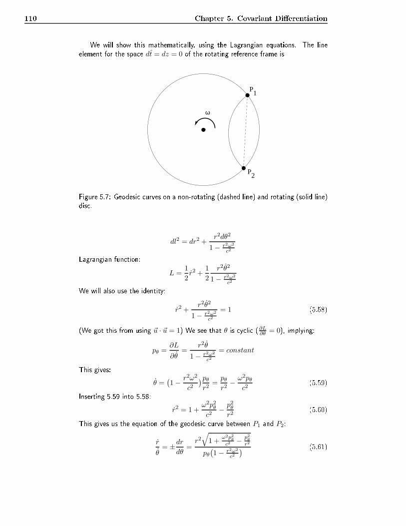
110 Chapter 5. Covariant DierentiationWe will show this mathemati ally, using the Lagrangian equations. The lineelement for the spa e dt = dz = 0 of the rotating referen e frame is

2

ω

P1

PFigure 5.7: Geodesi urves on a non-rotating (dashed line) and rotating (solid line)dis .dl2 = dr2 +

r2dθ2

1 − r2ω2

c2Lagrangian fun tion:L =

1

2r2 +

1

2

r2θ2

1 − r2ω2

c2We will also use the identity:r2 +

r2θ2

1 − r2ω2

c2

= 1 (5.58)(We got this from using ~u · ~u = 1) We see that θ is y li (∂L∂θ = 0), implying:pθ =

∂L

∂θ=

r2θ

1 − r2ω2

c2

= constantThis gives:θ =

(1 − r2ω2

c2)pθr2

=pθr2

− ω2pθc2

(5.59)Inserting 5.59 into 5.58:r2 = 1 +

ω2p2θ

c2− p2

θ

r2(5.60)This gives us the equation of the geodesi urve between P1 and P2:

r

θ= ±dr

dθ=r2√

1 +ω2p2

θ

c2− p2

θ

r2

pθ(1 − r2ω2

c2

) (5.61)

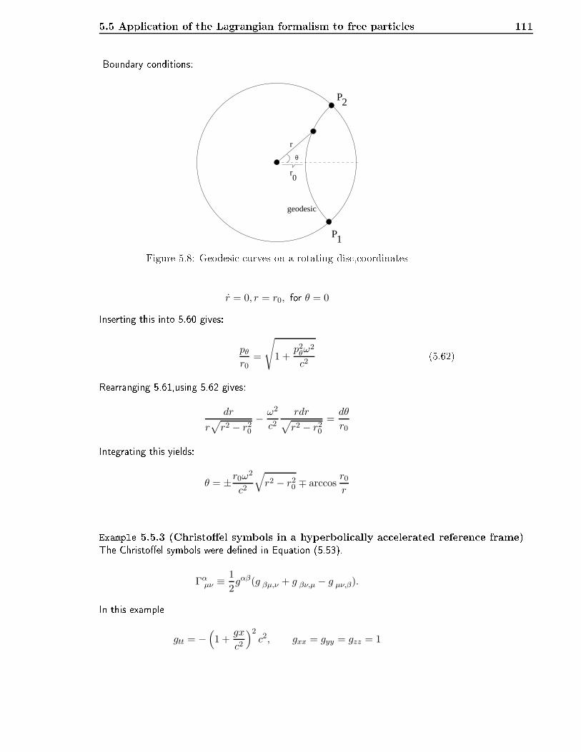
5.5 Appli ation of the Lagrangian formalism to free parti les 111Boundary onditions:2

θ

r

geodesic

r0

P1

P

Figure 5.8: Geodesi urves on a rotating dis , oordinatesr = 0, r = r0, for θ = 0Inserting this into 5.60 gives:

pθr0

=

√

1 +p2θω

2

c2(5.62)Rearranging 5.61,using 5.62 gives:

dr

r√r2 − r20

− ω2

c2rdr√r2 − r20

=dθ

r0Integrating this yields:θ = ±r0ω

2

c2

√r2 − r20 ∓ arccos

r0rExample 5.5.3 (Christoel symbols in a hyperboli ally a elerated referen e frame)The Christoel symbols were dened in Equation (5.53).

Γαµν ≡1

2gαβ(g βµ,ν + g βν,µ − g µν,β).In this example

gtt = −(1 +

gx

c2

)2c2, gxx = gyy = gzz = 1

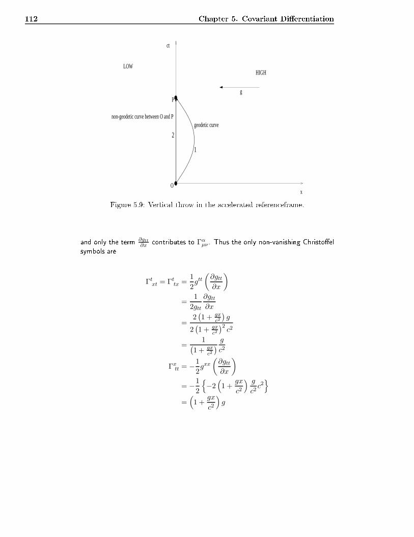
112 Chapter 5. Covariant Dierentiation

x

ct

Pg

O

non-geodetic curve between O and Pgeodetic curve

2

1

HIGHLOW

Figure 5.9: Verti al throw in the a elerated referen eframe.and only the term ∂gtt

∂x ontributes to Γαµν . Thus the only non-vanishing Christoelsymbols areΓtxt = Γttx =

1

2gtt(∂gtt∂x

)

=1

2gtt

∂gtt∂x

=2(1 + gx

c2

)g

2(1 + gx

c2

)2c2

=1(

1 + gxc2

) gc2

Γxtt = −1

2gxx

(∂gtt∂x

)

= −1

2

−2(1 +

gx

c2

) g

c2c2

=(1 +

gx

c2

)g

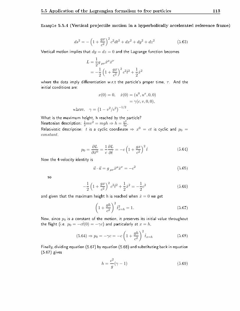
5.5 Appli ation of the Lagrangian formalism to free parti les 113Example 5.5.4 (Verti al proje tile motion in a hyperboli ally a elerated referen e frame)ds2 = −

(1 +

gx

c2

)2c2dt2 + dx2 + dy2 + dz2 (5.63)Verti al motion implies that dy = dz = 0 and the Lagrange fun tion be omes

L =1

2g µν x

µxν

= −1

2

(1 +

gx

c2

)2c2t2 +

1

2x2where the dots imply dierentiation w.r.t the parti le's proper time, τ . And theinitial onditions are:

x(0) = 0, x(0) = (u0, ux, 0, 0)

= γ(c, v, 0, 0),where, γ =(1 − v2/c2

)−1/2.What is the maximum height, h rea hed by the parti le?Newtonian des ription: 1

2mv2 = mgh⇒ h = v2

2g .Relativisti des ription: t is a y li oordinate ⇒ x0 = ct is y li and p0 =constant.

p0 =∂L

∂x0=

1

c

∂L

∂t= −c

(1 +

gx

c2

)2t (5.64)Now the 4-velo ity identity is

~u · ~u = g µν xµxν = −c2 (5.65)so

−1

2

(1 +

gx

c2

)2c2t2 +

1

2x2 = −1

2c2 (5.66)and given that the maximum height h is rea hed when x = 0 we get

(1 +

gh

c2

)2

t2x=h = 1. (5.67)Now, sin e p0 is a onstant of the motion, it preserves its initial value throughoutthe ight (i.e. p0 = −ct(0) = −γc) and parti ularly at x = h,(5.64) ⇒ p0 = −γc = −c

(1 +

gh

c2

)2

tx=h (5.68)Finally, dividing equation (5.67) by equation (5.68) and substituting ba k in equation(5.67) givesh =

c2

g(γ − 1) (5.69)

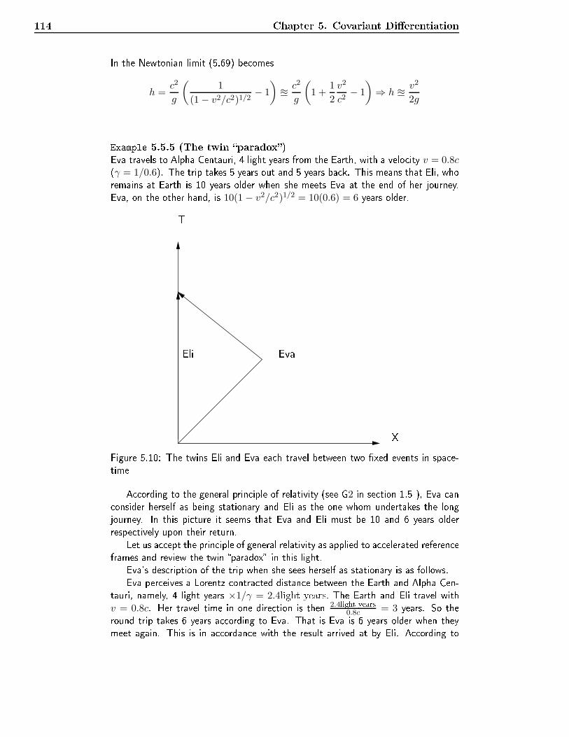
114 Chapter 5. Covariant DierentiationIn the Newtonian limit (5.69) be omesh =

c2

g

(1

(1 − v2/c2)1/2− 1

)≅c2

g

(1 +

1

2

v2

c2− 1

)⇒ h ≅

v2

2gExample 5.5.5 (The twin paradox)Eva travels to Alpha Centauri, 4 light years from the Earth, with a velo ity v = 0.8c(γ = 1/0.6). The trip takes 5 years out and 5 years ba k. This means that Eli, whoremains at Earth is 10 years older when she meets Eva at the end of her journey.Eva, on the other hand, is 10(1 − v2/c2)1/2 = 10(0.6) = 6 years older.TEvaEli

XFigure 5.10: The twins Eli and Eva ea h travel between two xed events in spa e-timeA ording to the general prin iple of relativity (see G2 in se tion 1.5 ), Eva an onsider herself as being stationary and Eli as the one whom undertakes the longjourney. In this pi ture it seems that Eva and Eli must be 10 and 6 years olderrespe tively upon their return.Let us a ept the prin iple of general relativity as applied to a elerated referen eframes and review the twin paradox in this light.Eva's des ription of the trip when she sees herself as stationary is as follows.Eva per eives a Lorentz ontra ted distan e between the Earth and Alpha Cen-tauri, namely, 4 light years ×1/γ = 2.4light years. The Earth and Eli travel withv = 0.8c. Her travel time in one dire tion is then 2.4light years

0.8c = 3 years. So theround trip takes 6 years a ording to Eva. That is Eva is 6 years older when theymeet again. This is in a ordan e with the result arrived at by Eli. A ording to

5.5 Appli ation of the Lagrangian formalism to free parti les 115Eva, Eli ages by only 6 years ×1/γ = 3.6 years during the round trip, not 10 yearsas Eli found.On turning about Eva experien es a for e whi h redu es her velo ity and a eler-ates her towards the Earth and Eli. This means that she experien es a gravitationalfor e dire ted away from the Earth. Eli is higher up in this gravitational eld andages faster than Eva, be ause of the gravitational time dilation. We assume thatEva has onstant proper a eleration and is stationary in a hyperboli ally a eleratedframe as she turns about.The anoni al momentum pt for Eli is then(see Equation (5.64))pt = −

(1 +

gx

c2

)2ctInserting this into the 4-velo ity identity gives

p2t − c2

(1 +

gx

c2

)2=(1 +

gx

c2

)2x2, (5.70)or

dτ =1 + gx

c2√p2t − c2

(1 + gx

c2

)2 dxNow, sin e x = 0 for x = x2 (x2 is Eli's turning point a ording to Eva), wehave thatpt = c

(1 +

gx2

c2

)Let x1 be Eli's position a ording to Eva just as Eva begins to noti e the gravitationaleld. That is when Eli begins to slow down in Eva's frame.Integration from x1 to x2 and inserting the value of pt givesτ1−2 =

c

g

√(1 +

gx2

c2

)2−(1 +

gx1

c2

)2

⇒ limg→∞

τ1−2 =1

c

√x2

2 − x21.Now setting x2 = 4 and x1 = 2.4 light years respe tively we get

limg→∞

τ1−2 = 3.2 yearsEli's aging as she turns about is, a ording to Eva,∆τEli = 2 lim

g→∞τ1−2 = 6.4 years.So Eli's has aged by a total of τEli = 3.6+ 6.4 = 10 years, a ording to Eva, whi his just what Eli herself found.

116 Chapter 5. Covariant Dierentiation5.5.3 Gravitational Doppler ee tThis on erns the frequen y shift of light traversing up or down in a gravitationaleld. The 4-momentum of a parti le with relativisti energy E and spatialvelo ity ~w (3-velo ity) is given by:~P = E(1, ~w) (c = 1) (5.71)Let ~U be the 4-velo ity of an observer. In a o-moving orthonormal basis of theobserver we have ~U = (1, 0, 0, 0). This gives

~U · ~P = −E (5.72)The energy of a parti le with 4-momentum ~P measured by an observer with4-velo ity ~U isE = −~U · ~P (5.73)Let ES = −(~U · ~P )S and Ea = −(~U · ~P )a be the energy of a photon, measuredlo ally by observers in rest in the transmitter and re eiver positions, respe tively.This gives1ES

(~U · ~P )S=

Ea

(~U · ~P )a(5.74)Let the angular frequen y of the light, measured by the transmitter and re eiver,be ws and wa, respe tively. We then have

ws =ES~, wa =

Ea~, (5.75)whi h gives:

wa =(~U · ~P )a

(~U · ~P )sws (5.76)For an observer at rest in a time-independent orthogonal metri we have

~U · ~P = U tPt =dt

dτPt (5.77)where Pt is a onstant of motion (sin e t is a y li oordinate) for photons andhen e has the same value in transmitter and re eiver positions. The line-elementis

ds2 = gttdt2 + gii(dx

i)2 (5.78)Using the physi al interpretation (5.55) of the line-element for a time like inter-val, we obtain for the proper time of an observer at restdτ2 = −gttdt2 ⇒ dτ =

√−gttdt (5.79)1 ~A · ~B = A0B0

+ A1B1

+ ... = g00A0B0

+ g11A1B1

+ ..., an orthonormal basis gives~A · ~B = −A0B0

+ A1B1+ ...

5.6 The Koszul onne tion 117Hen edt

dτ=

1√−gtt, (5.80)whi h gives

~U · ~P =1√−gtt

Pt. (5.81)Inserting this into the expression for angular frequen y (5.76) giveswa =

√(gtt)s(gtt)a

ws (5.82)Note: we have assumed an orthogonal and time-independent metri , i.e. Pt1 =Pt2 . Inserting the metri of a hyperboli ally a elerated referen e system with

gtt = −(1 +gx

c2)2 (5.83)gives

wa =1 + gxs

c2

1 + gxa

c2ws, (5.84)or

wa −wsws

=1 + gxs

c2

1 + gxa

c2− 1 =

gc2

(xs − xa)

1 + gxa

c2≈ g

c2H, (5.85)where H = xs− xa is the dieren e in height between transmitter and re eiver.Example 5.5.6 (Measurements of gravitational Doppler ee ts (Pound and Rebka 1960))

H ≈ 20m, g = 10m/s2gives∆w

w=

200

9 × 1016= 2.2 × 10−15.This ee t was measured by Pound and Rebka in 1960.5.6 The Koszul onne tionThe ovariant dire tional derivative of a s alar eld f in the dire tion of a ve tor

~u is dened as:∇~uf ≡ ~u(f) (5.86)Here the ve tor ~u should be taken as a dierensial operator. (In oordinatebasis, ~u = uµ ∂

∂xµ )The dire tional derivative along a basis ve tor ~eν is written as:∇ν ≡ ∇~eν

(5.87)Hen e ∇µ( ) = ∇~eµ( ) = ~eµ( )

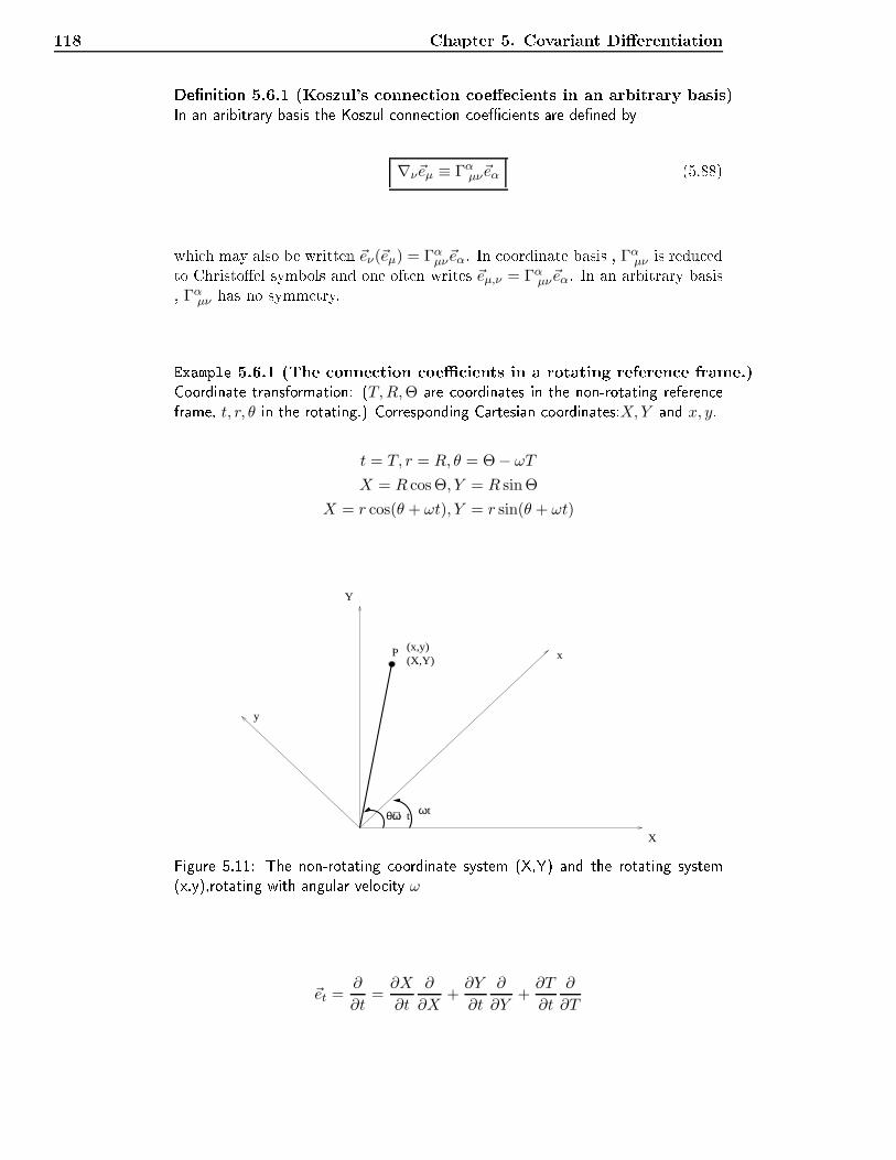
118 Chapter 5. Covariant DierentiationDenition 5.6.1 (Koszul's onne tion oee ients in an arbitrary basis)In an aribitrary basis the Koszul onne tion oe ients are dened by∇ν~eµ ≡ Γαµν~eα (5.88)whi h may also be written ~eν(~eµ) = Γαµν~eα. In oordinate basis , Γαµν is redu edto Christoel symbols and one often writes ~eµ,ν = Γαµν~eα. In an arbitrary basis, Γαµν has no symmetry.Example 5.6.1 (The onne tion oe ients in a rotating referen e frame.)Coordinate transformation: (T,R,Θ are oordinates in the non-rotating referen eframe, t, r, θ in the rotating.) Corresponding Cartesian oordinates:X,Y and x, y.

t = T, r = R, θ = Θ − ωT

X = R cos Θ, Y = R sin Θ

X = r cos(θ + ωt), Y = r sin(θ + ωt)

X

Y

t

y

xP (x,y)(X,Y)

ωtθ+ωFigure 5.11: The non-rotating oordinate system (X,Y) and the rotating system(x,y),rotating with angular velo ity ω~et =

∂

∂t=∂X

∂t

∂

∂X+∂Y

∂t

∂

∂Y+∂T

∂t

∂

∂T

5.6 The Koszul onne tion 119gives:~et = −rω sin(θ + ωt)~eX + rω cos(θ + ωt)~eY + ~eT

~er =∂X

∂r

∂

∂X+∂Y

∂r

∂

∂Y= cos(θ + ωt)~eX + sin(θ + ωt)~eY

~eθ =∂X

∂θ

∂

∂X+∂Y

∂θ

∂

∂Y= −r sin(θ + ωt)~eX + r cos(θ + ωt)~eYWe are going to nd the Christoel symbols, whi h involves dierentiation of ba-sis ve tors. This oordinate transformation makes this easy, sin e ~eX , ~eY , ~eT are onstant. Dierentiation gives

∇t~et = −rω2 cos(θ + ωt)~eX − rω2 sin(θ + ωt)~eY (5.89)The onne tion oe ients are (see eq. 5.88)∇ν~eµ ≡ Γαµν~eα (5.90)So, to al ulate Γαµν , the right hand side of eq.5.89 has to by expressed by thebasis that we are dierentiating.By inspe tion, the right hand side is −rω2~er.That is ∇t~et = −rω2~er giving Γrtt = −rω2.The other nonzero Christoel symbols are

Γθrt = Γθtr =ω

r,Γθθr = Γθrθ =

1

rΓrθt = Γrtθ = −rω,Γrθθ = −rExample 5.6.2 (A eleration in a non-rotating referen e frame (Newton))~r = ~v = (vi + Γiαβv

αvβ)~ei,where · ≡ ddt . i, j, and k are spa e indi es. Inserting the Christoel symbols forplane polar oordinates (see example 5.2.1), gives:

~ainert = (r − rθ2)~er + (θ +2

rrθ)~eθExample 5.6.3 (The a eleration of a parti le, relative to the rotating referen e frame)Inserting the Christoel symbols from example 5.6.1:

~arot = (r − rθ2 − Γrttt2 + Γrθtθt+ Γrtθ tθ)~er + (θ +

2

rrθ + Γθrtrt+ Γθtr tr)~eθ

= (r − rθ2 − rω2 − 2rωθ)~er + (rθ + 2rθ + 2rω)~eθ

= ~ainert − (rω2 + 2rωθ)~er + 2rω~eθ

120 Chapter 5. Covariant DierentiationThe angular velo ity of the referen e frame, is ~ω = ω~ez. We also introdu e ~r = r~er.The velo ity relative to the rotating referen e frame is then:~r = r~er + r~erFurthermore

~er =d~erdt

=∂~er∂xi

dxi

dt= vi~er,iUsing denition 5.6.1 in a oordinate basis, this may be written

~er = viΓjri~ejUsing the expressions of the Christoel symbols in example 5.6.1, we get~er = vθΓθrθ~eθ = θ

1

r~eθ = θ~eθHen e

~v = ~r = r~er + rθ~eθInserting this into the expression for the a eleration, gives:~rrot = ~rinert + ~ω × (~ω × ~r) + 2~ω × ~vWe an see that the entrifugal a eleration (the term in the middle) and the oriolisa eleration (last term) is ontained in the expression for the ovariant derivative.5.7 Conne tion oe ients Γαµν and stru ture oe- ients cαµν in a Riemannian (torsion free) spa eThe ommutator of two ve tors, ~u and ~v, expressed by ovariant dire tionalderivatives is given by:

[~u,~v] = ∇~u~v −∇~v~u (5.91)Let ~u = ~eµ and ~v = ~eν . We then have:[ ~eµ, ~eν ] = ∇µ ~eν −∇ν ~eµ. (5.92)Using the denitions of the onne tion and stru ture oe ients we get:cαµν ~eα = (Γανµ − Γαµν) ~eα (5.93)Thus in a torsion free spa e

cαµν = Γανµ − Γαµν (5.94)In oordinate basis we have~eµ =

∂

∂xµ, ~eν =

∂

∂xν(5.95)

5.8 Covariant dierentiation of ve tors, forms and tensors 121And therefore:[ ~eµ, ~eν ] = [

∂

∂xµ,∂

∂xν]

=∂

∂xµ(∂

∂xν) − ∂

∂xν(∂

∂xµ)

=∂2

∂xµ∂xν− ∂2

∂xν∂xµ= 0

(5.96)Equation (5.96) shows that cαµν = 0, and that the onne tion oe ients inEquation (5.94) therefore are symmetri al in a oordinate basis:Γανµ = Γαµν (5.97)5.8 Covariant dierentiation of ve tors, forms and ten-sors5.8.1 Covariant dierentiation of a ve tor in an arbitrary basis

∇ν ~A = ∇ν(Aµ ~eµ)= ∇νAµ ~eµ +Aα∇ν ~eα

(5.98)∇νAµ = ~eν(A

µ) , ~eν = Mµν

∂

∂xµ, (5.99)where Mµ

ν are the elements of a transformation matrix between a oordinatebasis ∂∂xµ and an arbitrary basis ~eν. ( If ~eν had been a oordinate basisve tor, we would have gotten ~eν(A

µ) = ∂∂xν (Aµ) = Aµ,ν).

∇ν ~A = [~eν(Aµ) +AαΓµαν ] ~eµ (5.100)Denition 5.8.1 (Covariant derivative of a ve tor)The ovariant derivative of a ve tor in an arbitrary basis is dened by:

∇ν ~A ≡ Aµ;ν~eµ (5.101)So:Aµ;ν = ~eν(A

µ) +AαΓµαν

where ∇ν~eα ≡ Γµαν~eµ(5.102)

5.8.2 Covariant dierentiation of formsDenition 5.8.2 (Covariant dire tional derivative of a one-form eld)Given a ve tor eld ~A and a one-form eld α, the ovariant dire tional derivative ofα in the dire tion of the ve tor ~u is dened by:

(∇~uα)( ~A ) ≡ ∇~u[α( ~A )︸ ︷︷ ︸αµAµ

] − α(∇~u ~A) (5.103)

122 Chapter 5. Covariant DierentiationLet α = ωµ (basis form), ωµ(~eν) ≡ δµν and let ~A = ~eν and ~u = ~eλ. We thenhave:(∇λωµ)(~eν) = ∇λ[ωµ(~eν)︸ ︷︷ ︸

δµν

] − ωµ(∇λ ~eν) (5.104)The ovariant dire tional derivative ∇λ of a onstant s alar eld is zero, ∇λδµν =0. We therefore get:

(∇λωµ)(~eν) = −ωµ(∇λ ~eν)= −ωµ(Γανλ ~eα)

= −Γανλωµ( ~eα)

= −Γανλδµα

= −Γµνλ

(5.105)The ontra tion between a one-form and a basis ve tor gives the omponentsof the one-form, α(~eν) = αν . Equation (5.105) tells us that the ν- omponent of∇λωµ is equal to −Γµνλ, and that we therefore have

∇λωµ = −Γµνλων (5.106)Equation (5.106) gives the dire tional derivatives of the basis forms. Using theprodu t of dierentiation gives

∇λα = ∇λ(αµωµ)= ∇λ(αµ)ωµ + αµ∇λωµ

= ~eλ(αµ)ωµ − αµΓ

µνλω

ν

(5.107)Denition 5.8.3 (Covariant derivative of a one-form)The ovariant derivative of a one-form α = αµω

µ is therefore given by Equation(5.108) below, when we let µ→ ν in the rst term on the right hand side in (5.107):∇λα = [ ~eλ(αν) − αµΓ

µνλ]ω

ν (5.108)The ovariant derivative of the one-form omponents αµ are denoted by αν;λ andare dened by∇λα ≡ αν;λω

ν (5.109)It then follows thatαν;λ = ~eλ(αν) − αµΓ

µνλ (5.110)It is worth to note that Γµνλ in Equation (5.110) are not Christoel symbols. In oordinate basis we get:

αν;λ = αν,λ − ανΓµλν (5.111)where Γµλν = Γµνλ are Christoel symbols.

5.9 The Cartan onne tion 1235.8.3 Generalization for tensors of higher rankDenition 5.8.4 (Covariant derivative of a tensor)Let A and B be two tensors of arbitrary rank. The ovariant dire tional derivativealong a basis ve tor ~eλ of a tensor A⊗B of arbitrary rank is dened by:∇λ(A⊗B) ≡ (∇λA) ⊗B +A⊗ (∇λB) (5.112)We will use (5.112) to nd the formula for the ovariant derivative of the om-ponents of a tensor of rank 2:

∇αS = ∇α(Sµνωµ ⊗ ων)

= (∇αSµν)ωµ ⊗ ων + Sµν(∇αωµ) ⊗ ων + Sµνωµ ⊗ (∇αων)

= (Sµν,α − SβνΓβµα − SµβΓ

βνα)ωµ ⊗ ων

(5.113)where Sµν,α = ~eα(Sµν). Dening the ovariant derivative Sµν;α by∇αS = Sµν;αω

µ ⊗ ων (5.114)we getSµν;α = Sµν,α − SβνΓ

βµα − SµβΓ

βνα (5.115)For the metri tensor we get

gµν;α = gµν,α − gβνΓβµα − gµβΓ

βνα (5.116)From

gµν = ~eµ · ~eν (5.117)we get:gµν,α = (∇α ~eµ) · ~eν + ~eµ(∇α ~eν)

= Γβµα ~eβ · ~eν + ~eµ · Γβνα ~eβ= gβνΓ

βµα + gµβΓ

βνα

(5.118)This means thatgµν;α = 0 (5.119)So the metri tensor is a ( ovariant) onstant tensor.5.9 The Cartan onne tionDenition 5.9.1 (Exterior derivative of a basis ve tor)

d~eµ ≡ Γνµα~eν ⊗ ωα (5.120)

124 Chapter 5. Covariant DierentiationExterior derivative of a ve tor eld:d ~A = d(~eµA

µ) = ~eν ⊗ dAν +Aµd~eµ (5.121)In arbitrary basis:dAν = ~eλ(A

ν)ωλ (5.122)(In oordinate basis, ~eλ(Aν) = ∂∂xλ (Aν) = Aν,λ)giving:

d ~A = ~eν ⊗ [~eλ(Aν)ωλ] +AµΓνµλ~eν ⊗ ωλ

= (~eλ(Aν) +AµΓνµλ)~eν ⊗ ωλ

(5.123)d ~A = Aν;λ~eν ⊗ ωλ (5.124)Denition 5.9.2 (Conne tion forms Ων

µ)The onne tion forms Ωνµ are 1-forms, dened by:

d~eµ ≡ ~eν ⊗ Ωνµ

Γνµα~eν ⊗ ωα = ~eν ⊗ Γνµαωα = ~eν ⊗ Ων

µ

(5.125)Ωνµ = Γνµαω

α (5.126)The exterior derivatives of the omponents of the metri tensor:dgµν = d(~eµ · ~eν) = ~eµ · d~eν + ~eν · d~eµ (5.127)where the meaning of the dot is dened as follows:Denition 5.9.3 (S alar produ t between ve tor and 1-form)The s alar produ t between a ve tor ~u and a (ve torial) one form A = Aµν~eµ ⊗ ωνis dened by:

~u · A ≡ uαAµν(~eα · ~eµ)ων (5.128)Using this denition, we get:dgµν = (~eµ · ~eλ)Ωλ

ν + (~eν · ~eγ)Ωγµ

= gµλΩλν + gνγΩ

γµ

(5.129)

5.9 The Cartan onne tion 125Lowering an index givesdgµν = Ωµν + Ωνµ (5.130)In an orthonormal basis eld there is Minkowski-metri :

gµν = ηµν (5.131)whi h is onstant. Then we have :dgµν = 0 ⇒ Ωνµ = −Ωµν (5.132)where we write Ωνµ = Γνµαω

α. It follows that Γνµα = −Γµνα.It also follows thatΓtij

= −Γtij = Γitj = Γitj

Γijk

= −Γjik

(5.133)Cartans 1st stru ture equation (without proof):dωρ = −1

2cρµνω

µ ∧ ων

= −1

2(Γρνµ − Γρµν)ω

µ ∧ ων

= −Γρνµωµ ∧ ων

= −Ωρν ∧ ων

(5.134)dωρ = −Ωρν ∧ ων and dωρ = Γρµνω

µ ∧ ων (5.135)In oordinate basis, we have ωρ = dxρ.Thus, dωρ = d2xρ = 0.We also have cρµν = 0 , and C1 is redu ed to an identity.This formalism annot be used in oordinate basis!Example 5.9.1 (Cartan- onne tion in an orthonormal basis eld in plane polar oord.)ds2 = dr2 + r2dθ2Introdu ing basis forms in an orthonormal basis eld (where the metri is grr =

gθθ = 1):ds2 = grrω

r ⊗ ωr + gθθωθ ⊗ ωθ = ωr ⊗ ωr + ωθ ⊗ ωθ

⇒ ωr = dr, ωθ = rdθExterior dierentiation gives:dωr = d2r = 0, dωθ = dr ∧ dθ =

1

rωr ∧ ωθ

126 Chapter 5. Covariant DierentiationC1:dωµ = −Ωµ

ν ∧ ων

= −Ωµr ∧ ωr − Ωµ

θ∧ ωθWe have that dωr = 0 , whi h gives:

Ωrθ

= Γrθθωθ (5.136)sin e ωθ ∧ ωθ = 0. (Ωr

r=0 be ause of the antisymmetry Ωνµ = −Ωµν .)We also have: dωθ = −1rω

θ ∧ ωr. C1:dωθ = −Ωθr ∧ ωr − Ωθ

θ︸︷︷︸=0

∧ωθ

Ωθr = Γθ

rθωθ + Γθrrω

r (5.137)giving Γθrθ

= 1r .We have: Ωr

θ= −Ωθr. Using equations 5.136 and 5.137 we get:

Γθrr = 0

⇒ Γrθθ

= −1

rgiving Ωrθ

= −Ωθr = −1

rωθ.

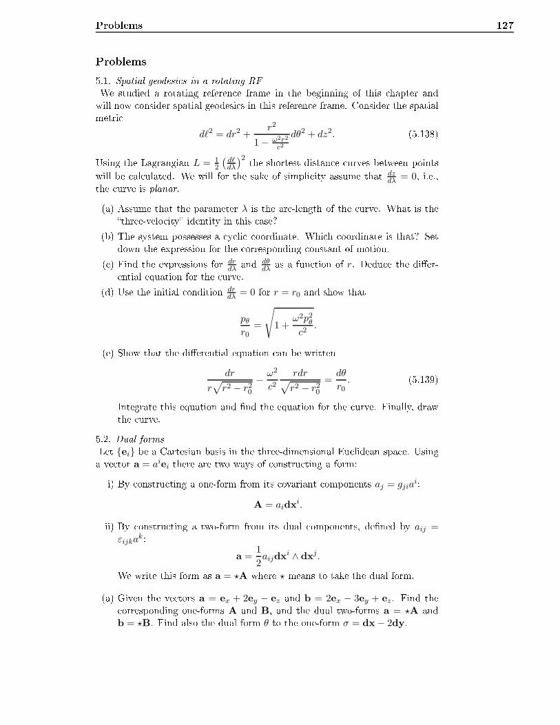
Problems 127Problems5.1. Spatial geodesi s in a rotating RFWe studied a rotating referen e frame in the beginning of this hapter andwill now onsider spatial geodesi s in this referen e frame. Consider the spatialmetri dℓ2 = dr2 +

r2

1 − ω2r2

c2

dθ2 + dz2. (5.138)Using the Lagrangian L = 12

(dℓdλ

)2 the shortest distan e urves between pointswill be al ulated. We will for the sake of simpli ity assume that dzdλ = 0, i.e.,the urve is planar.(a) Assume that the parameter λ is the ar -length of the urve. What is thethree-velo ity identity in this ase?(b) The system possesses a y li oordinate. Whi h oordinate is that? Setdown the expression for the orresponding onstant of motion.( ) Find the expressions for dr

dλ and dθdλ as a fun tion of r. Dedu e the dier-ential equation for the urve.(d) Use the initial ondition dr

dλ = 0 for r = r0 and show thatpθr0

=

√

1 +ω2p2

θ

c2.(e) Show that the dierential equation an be written

dr

r√r2 − r20

− ω2

c2rdr√r2 − r20

=dθ

r0. (5.139)Integrate this equation and nd the equation for the urve. Finally, drawthe urve.5.2. Dual formsLet ei be a Cartesian basis in the three-dimensional Eu lidean spa e. Usinga ve tor a = aiei there are two ways of onstru ting a form:i) By onstru ting a one-form from its ovariant omponents aj = gjia

i:A = aidxi.ii) By onstru ting a two-form from its dual omponents, dened by aij =

εijkak:

a =1

2aijdxi ∧ dxj.We write this form as a = ⋆A where ⋆ means to take the dual form.(a) Given the ve tors a = ex + 2ey − ez and b = 2ex − 3ey + ez. Find the orresponding one-forms A and B, and the dual two-forms a = ⋆A and

b = ⋆B. Find also the dual form θ to the one-form σ = dx− 2dy.

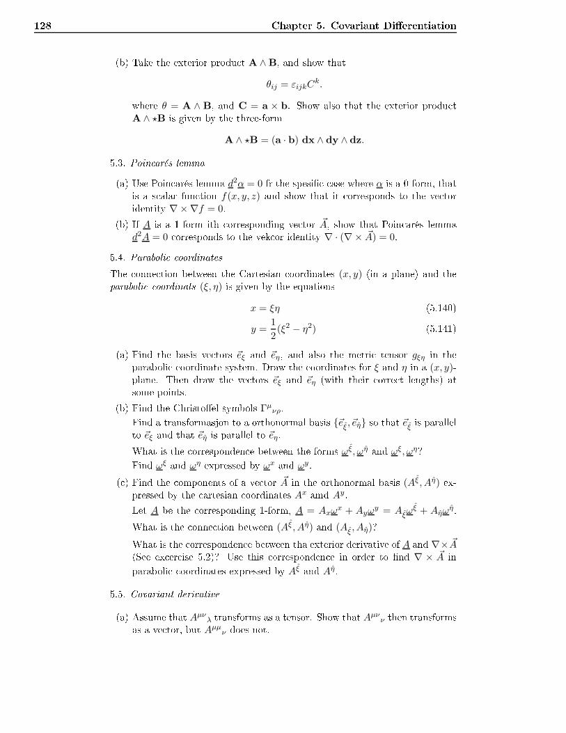
128 Chapter 5. Covariant Dierentiation(b) Take the exterior produ t A ∧ B, and show thatθij = εijkC

k.where θ = A ∧ B, and C = a × b. Show also that the exterior produ tA ∧ ⋆B is given by the three-form

A ∧ ⋆B = (a · b) dx ∧ dy ∧ dz.5.3. Poin arés lemma(a) Use Poin arés lemma d2α = 0 fr the spesi ase where α is a 0-form, thatis a s alar fun tion f(x, y, z) and show that it orresponds to the ve toridentity ∇×∇f = 0.(b) If A is a 1-form ith orresponding ve tor ~A, show that Poin arés lemmad2A = 0 orresponds to the vek or identity ∇ · (∇× ~A) = 0.5.4. Paraboli oordinatesThe onne tion between the Cartesian oordinates (x, y) (in a plane) and theparaboli oordinats (ξ, η) is given by the equations

x = ξη (5.140)y =

1

2(ξ2 − η2) (5.141)(a) Find the basis ve tors ~eξ and ~eη, and also the metri tensor gξη in theparaboli oordinate system. Draw the oordinates for ξ and η in a (x, y)-plane. Then draw the ve tors ~eξ and ~eη (with their orre t lengths) atsome points.(b) Find the Christoel symbols Γµνρ.Find a transformasjon to a orthonormal basis ~eξ , ~eη so that ~eξ is parallelto ~eξ and that ~eη is parallel to ~eη.What is the orresponden e between the forms ωξ, ωη and ωξ, ωη?Find ωξ and ωη expressed by ωx and ωy.( ) Find the omponents of a ve tor ~A in the orthonormal basis (Aξ , Aη) ex-pressed by the artesian oordinates Ax amd Ay.Let A be the orresponding 1-form, A = Axω

x + Ayωy = Aξω

ξ + Aηωη.What is the onne tion between (Aξ , Aη) and (Aξ , Aη)?What is the orresponden e between tha exterior derivative of A and ∇× ~A(See ex er ise 5.2)? Use this orresponden e in order to nd ∇ × ~A inparaboli oordinates expressed by Aξ and Aη.5.5. Covariant derivative(a) Assume that Aµνλ transforms as a tensor. Show that Aµνν then transformsas a ve tor, but Aµµν does not.

Problems 129(b) Show, by using the expressionΓµνλ =

1

2(gµν,λ + gµλ,ν − gνλ,µ) (5.142)that Γµνλ is not a tensor.( ) Assume that Aµ(x) is a ve tor eld. Show that Aµ,ν = ∂Aµ

∂xν does nottransform as a tensor, but that the ovariant derivativee,Aµ;ν = Aµ,ν + ΓµανA

α, (5.143)does.(d) Show thatgµν;λ = 0. (5.144)(e) Show that ovariant derivative satises the following:

(AµBν);λ = Aµ;λBν +AµBν;λ. (5.145)(f) Show that the ovarinat derivative an be expressed as∇ · ~A ≡ Aµ;µ =

1√|g|∂µ

(√|g|Aµ

), (5.146)where now g is the determinant of the metri tensor, g = det(gµν). (Hint:Use that ∂αg ≡ g,α = g gµνgµν,α.)5.6. Geodeti urves in spa e(a) In the two-dimensional Eu lidean plane the line-element is given by ds2 =

dx2 + dy2. A urve y = y(x) onne ts two points A and B in the plane.The distan e between A and B along the urve is thereforeS =

∫ B

Ads =

∫ B

A

[1 +

(dy

dx

)2] 1

2

dx. (5.147)If we vary the shape of this urve slightly, but keeping the end pointsA and B xed, it would lead to a hange δS of the length of the urve.Whenever δS = 0 for all small arbitrary variations with respe t to a given urve, then the urve is a geodeti urve. Find the Euler-Lagrange equationwhi h orresponds to δS = 0 and show that geodeti urves in the planeare straight lines.(b) A parti le with mass m is moving without fri tion on a two-dimensionalsurfa e embedded in the three-dimensional spa e. Write down the expres-sions for the Lagrangian, L, and the orresponding Euler-Lagrange equa-tions for the parti le. Show that L is a onstant of motion and explain thisby referring to the for es a ting on the parti le.The geodeti urves are found by variation of S =

∫ BA ds. Show, usingthe Euler-Lagrange equations, that the parti le is moving along a geodeti urve with onstant speed.

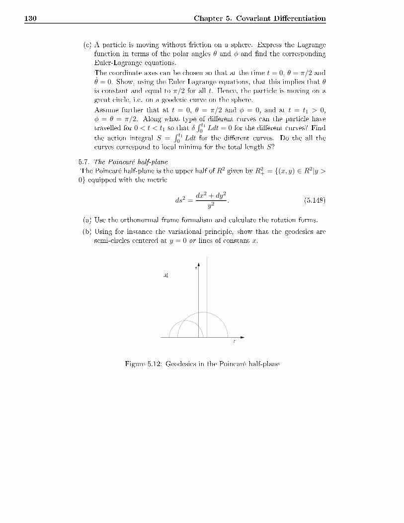
130 Chapter 5. Covariant Dierentiation( ) A parti le is moving without fri tion on a sphere. Express the Lagrangefun tion in terms of the polar angles θ and φ and nd the orrespondingEuler-Lagrange equations.The oordinate axes an be hosen so that at the time t = 0, θ = π/2 andθ = 0. Show, using the Euler-Lagrange equations, that this implies that θis onstant and equal to π/2 for all t. Hen e, the parti le is moving on agreat ir le, i.e. on a geodeti urve on the sphere.Assume further that at t = 0, θ = π/2 and φ = 0, and at t = t1 > 0,φ = θ = π/2. Along what type of dierent urves an the parti le havetravelled for 0 < t < t1 so that δ ∫ t10 Ldt = 0 for the dierent urves? Findthe a tion integral S =

∫ t10 Ldt for the dierent urves. Do the all the urves orrespond to lo al minima for the total length S?5.7. The Poin aré half-planeThe Poin aré half-plane is the upper half of R2 given by R2

+ = (x, y) ∈ R2|y >0 equipped with the metri

ds2 =dx2 + dy2

y2. (5.148)(a) Use the orthonormal frame formalism and al ulate the rotation forms.(b) Using for instan e the variational prin iple, show that the geodesi s aresemi- ir les entered at y = 0 or lines of onstant x.

x

yR2+

Figure 5.12: Geodesi s in the Poin aré half-plane

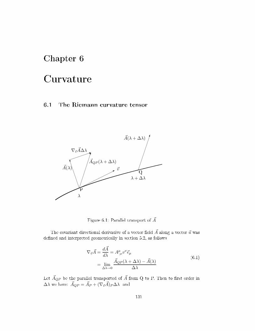
Chapter 6Curvature6.1 The Riemann urvature tensor

*

M

1

P Qλ

λ+ ∆λ

~A(λ)

~AQP (λ+ ∆λ)

∇~v~A∆λ

~v

~A(λ+ ∆λ)

Figure 6.1: Parallel transport of ~AThe ovariant dire tional derivative of a ve tor eld ~A along a ve tor ~u wasdened and interpreted geometri ally in se tion 5.2, as follows∇~v

~A =d ~A

dλ= Aµ;νv

ν~eµ

= lim∆λ→0

~AQP (λ+ ∆λ) − ~A(λ)

∆λ

(6.1)Let ~AQP be the parallel transported of ~A from Q to P. Then to rst order in∆λ we have: ~AQP = ~AP + (∇~v

~A)P∆λ and 131

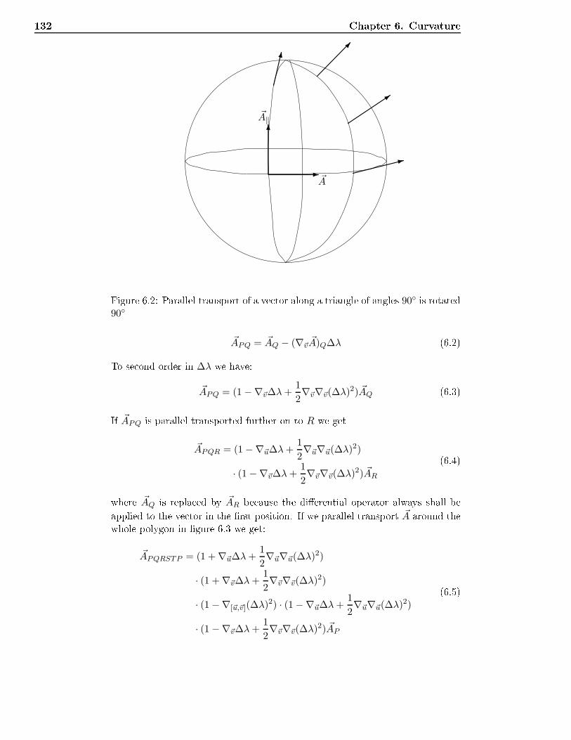
132 Chapter 6. Curvature

-~A

6

~A‖

:

3

Figure 6.2: Parallel transport of a ve tor along a triangle of angles 90 is rotated90

~APQ = ~AQ − (∇~v~A)Q∆λ (6.2)To se ond order in ∆λ we have:

~APQ = (1 −∇~v∆λ+1

2∇~v∇~v(∆λ)2) ~AQ (6.3)If ~APQ is parallel transported further on to R we get

~APQR = (1 −∇~u∆λ+1

2∇~u∇~u(∆λ)2)

· (1 −∇~v∆λ+1

2∇~v∇~v(∆λ)2) ~AR

(6.4)where ~AQ is repla ed by ~AR be ause the dierential operator always shall beapplied to the ve tor in the rst position. If we parallel transport ~A around thewhole polygon in gure 6.3 we get:~APQRSTP = (1 + ∇~u∆λ+

1

2∇~u∇~u(∆λ)2)

· (1 + ∇~v∆λ+1

2∇~v∇~v(∆λ)2)

· (1 −∇[~u,~v](∆λ)2) · (1 −∇~u∆λ+1

2∇~u∇~u(∆λ)2)

· (1 −∇~v∆λ+1

2∇~v∇~v(∆λ)2) ~AP

(6.5)

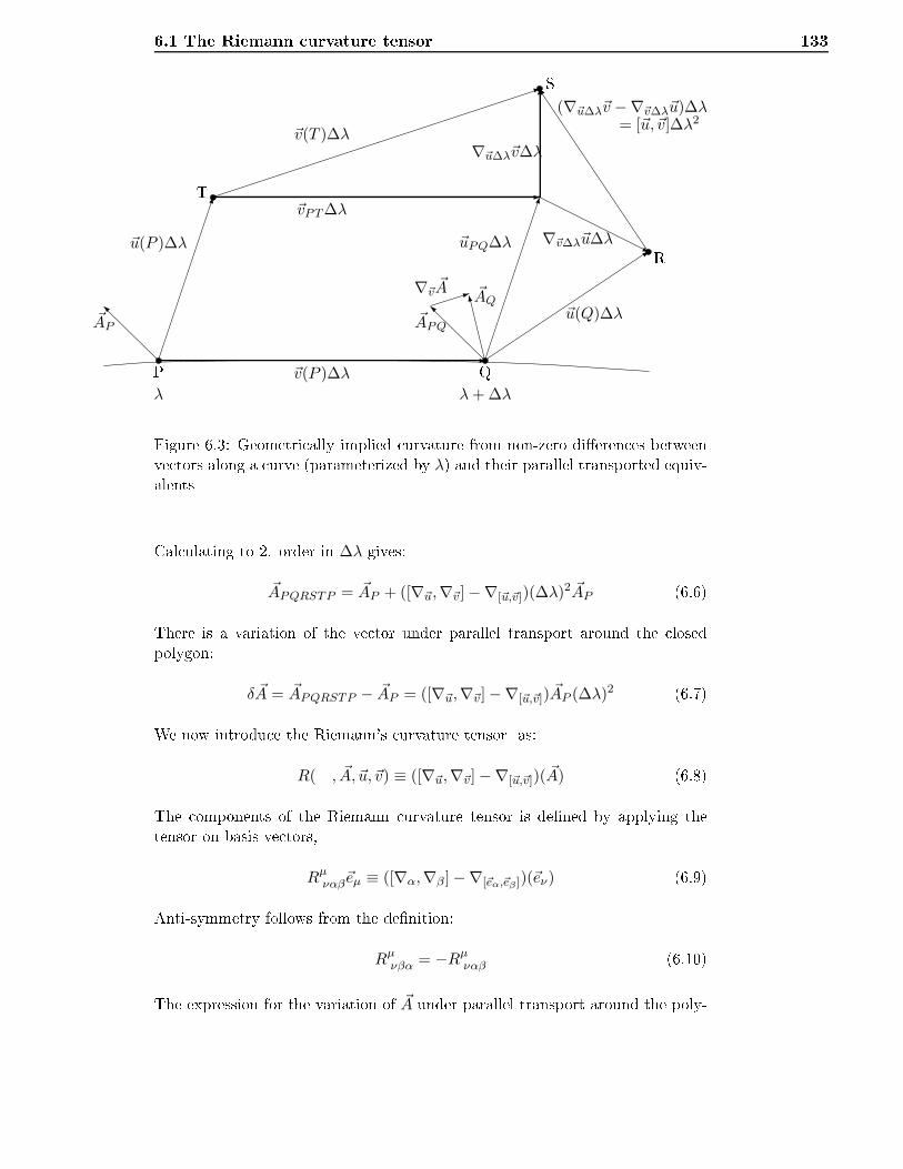
6.1 The Riemann urvature tensor 133

-

3

]1

-

6

j

I IO

1Pλ

Qλ+ ∆λ

RS

T (∇~u∆λ~v −∇~v∆λ~u)∆λ= [~u,~v]∆λ2

∇~v∆λ~u∆λ

∇~u∆λ~v∆λ

~u(P )∆λ

~AP

~uPQ∆λ

~APQ

~AQ∇~v

~A

~v(P )∆λ

~vPT∆λ

~v(T )∆λ

~u(Q)∆λ

Figure 6.3: Geometri ally implied urvature from non-zero dieren es betweenve tors along a urve (parameterized by λ) and their parallel transported equiv-alentsCal ulating to 2. order in ∆λ gives:~APQRSTP = ~AP + ([∇~u,∇~v] −∇[~u,~v])(∆λ)2 ~AP (6.6)There is a variation of the ve tor under parallel transport around the losedpolygon:

δ ~A = ~APQRSTP − ~AP = ([∇~u,∇~v ] −∇[~u,~v]) ~AP (∆λ)2 (6.7)We now introdu e the Riemann's urvature tensor as:R( , ~A, ~u,~v) ≡ ([∇~u,∇~v] −∇[~u,~v])( ~A) (6.8)The omponents of the Riemann urvature tensor is dened by applying thetensor on basis ve tors,Rµναβ~eµ ≡ ([∇α,∇β ] −∇[~eα,~eβ ])(~eν) (6.9)Anti-symmetry follows from the denition:

Rµνβα = −Rµναβ (6.10)The expression for the variation of ~A under parallel transport around the poly-

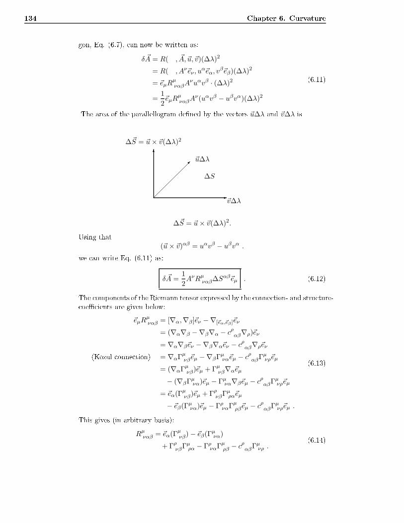
134 Chapter 6. Curvaturegon, Eq. (6.7), an now be written as:δ ~A = R( , ~A, ~u,~v)(∆λ)2

= R( , Aν~eν , uα~eα, v

β~eβ)(∆λ)2

= ~eµRµναβA

νuαvβ · (∆λ)2

=1

2~eµR

µναβA

ν(uαvβ − uβvα)(∆λ)2

(6.11)The area of the parallellogram dened by the ve tors ~u∆λ and ~v∆λ is-

6

~v∆λ

~u∆λ

∆~S = ~u× ~v(∆λ)2

∆S

∆~S = ~u× ~v(∆λ)2.Using that(~u× ~v)αβ = uαvβ − uβvα .we an write Eq. (6.11) as:δ ~A =

1

2AνRµναβ∆S

αβ~eµ . (6.12)The omponents of the Riemann tensor expressed by the onne tion- and stru ture- oe ients are given below:~eµR

µναβ = [∇α,∇β]~eν −∇[~eα,~eβ ]~eν

= (∇α∇β −∇β∇α − cραβ∇ρ)~eν

= ∇α∇β~eν −∇β∇α~eν − cραβ∇ρ~eν(Kozul- onne tion) = ∇αΓµνβ~eµ −∇βΓ

µνα~eµ − cραβΓ

µνρ~eµ

= (∇αΓµνβ)~eµ + Γµνβ∇α~eµ

− (∇βΓµνα)~eµ − Γµνα∇β~eµ − cραβΓ

µνρ~eµ

= ~eα(Γµνβ)~eµ + ΓρνβΓµρα~eµ

− ~eβ(Γµνα)~eµ − ΓρναΓ

µρβ~eµ − cραβΓ

µνρ~eµ .

(6.13)This gives (in arbitrary basis):

Rµναβ = ~eα(Γµνβ) − ~eβ(Γ

µνα)

+ ΓρνβΓµρα − ΓρναΓµρβ − cραβΓ

µνρ .

(6.14)

6.1 The Riemann urvature tensor 135In oordinate basis eq. (6.14) is redu ed to:Rµναβ = Γµνβ,α − Γµνα,β + ΓρνβΓ

µρα − ΓρναΓ

µρβ , (6.15)where Γµνβ = Γµβν are the Christoel symbols.Due to the antisymmetry (6.10) we an dene a matrix of urvature-forms

Rµν =1

2Rµναβω

α ∧ ωβ (6.16)Inserting the omponents of the Riemann tensor from eq. (6.14) givesRµν = (~eα(Γµνβ) + ΓρνβΓ

µρα − 1

2cραβΓ

µνρ)ω

α ∧ ωβ (6.17)The onne tion forms:Ωµν = Γµναω

α (6.18)Exterior derivatives of basis forms:dωρ = −1

2cραβω

α ∧ ωβ (6.19)Exterior derivatives of onne tion forms (C1: dωρ = −Ωρα ∧ ωα) :dΩµ

ν = dΓµνβ ∧ ωβ + Γµνρdωρ

= ~eα(Γµνβ)ωα ∧ ωβ − 1

2cραβΓ

µνρω

α ∧ ωβ(6.20)The urvature forms an now be written as:

Rµν = dΩµν + Ωµλ ∧ Ωλ

ν (6.21)This is Cartans 2nd stru ture equation.

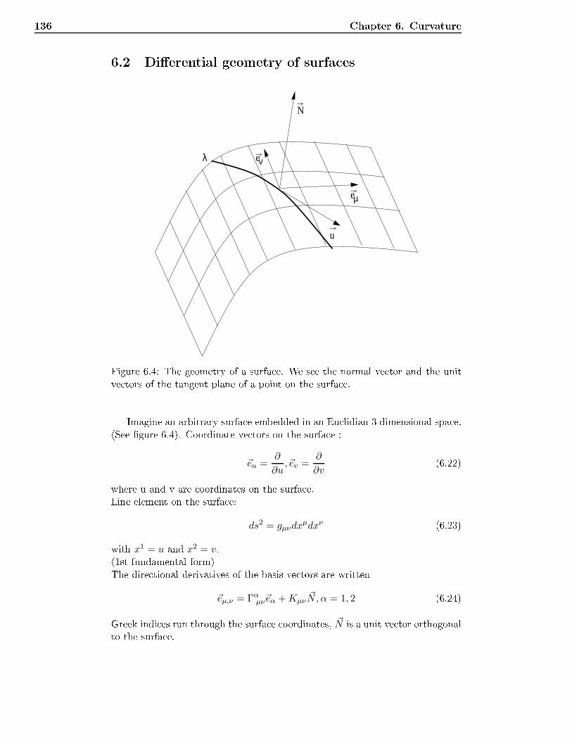
136 Chapter 6. Curvature6.2 Dierential geometry of surfa esλ

µe

eν

N

u

Figure 6.4: The geometry of a surfa e. We see the normal ve tor and the unitve tors of the tangent plane of a point on the surfa e.Imagine an arbitrary surfa e embedded in an Eu lidian 3 dimensional spa e.(See gure 6.4). Coordinate ve tors on the surfa e :~eu =

∂

∂u,~ev =

∂

∂v(6.22)where u and v are oordinates on the surfa e.Line element on the surfa e:

ds2 = gµνdxµdxν (6.23)with x1 = u and x2 = v.(1st fundamental form)The dire tional derivatives of the basis ve tors are written

~eµ,ν = Γαµν~eα +Kµν~N,α = 1, 2 (6.24)Greek indi es run through the surfa e oordinates, ~N is a unit ve tor orthogonalto the surfa e.

6.2 Dierential geometry of surfa es 137The equation above is alled Gauss' equation. We have: Kµν = ~eµ,ν · ~N . In oordinate basis, we have ~eµ,ν = ∂2

∂xµ∂xν = ∂2

∂xν∂xµ = ~eν,µ. It follows thatKµν = Kνµ (6.25)Let ~u be the unit tangent ve tor to a urve on the surfa e, parametrised by λ.Dierentiating ~u along the urve:

d~u

dλ= uµ;νu

ν~eµ + Kµνuµuν︸ ︷︷ ︸2nd fundamental form ~N (6.26)We dene κg and κN by:

d~u

dλ= κg~e+ κN ~N (6.27)

κg is alled geodesi urvature. κN is alled normal urvature (external urva-ture). κg = 0 for geodesi urves on the surfa e.κg~e = uµ;νu

ν~eµ = ∇~u~u

κN = KµνuµuνAnd :κN =

d~u

dλ· ~N

(6.28)We also have that ~u · ~N = 0 along the whole urve. Dierentiation gives:d~u

dλ· ~N + ~u · d

~N

dλ= 0 (6.29)gives:

κN = −~u · d~N

dλ(6.30)whi h is alled Weingarten's equation.

κg and κN together give a omplete des ription of the geometry of a surfa ein a at 3 dimensional spa e. We are now going to onsider geodesi urvesthrough a point on the surfa e. Tangent ve tor ~u = uµ~eµ with ~u ·~u = gµνuµuν =

1. Dire tions with maximum and minimum values for the normal urvatures arefound, by extremalizing κN under the ondition gµνuµuν = 1. We then solve thevariation problem δF = 0 for arbitrary uµ, where F = Kµνuµuν−k(gµνuµuν−1).Here k is the Lagrange multipli ator. Variation with respe t to uµ gives:

δF = 2(Kµν − kgµν)uνδuµ

δF = 0 for arbitrary δuµ demands:(Kµν − kgµν)u

ν = 0 (6.31)For this system of equations to have nonzero solutions, we must have:det(Kµν − kgµν) = 0 (6.32)

138 Chapter 6. Curvature∣∣∣∣K11 − kg11 K12 − kg12K21 − kg21 K22 − kg22

∣∣∣∣ = 0 (6.33)This gives the following quadrati equation for k:k2det(gµν) − (g11K22 − 2g12K12 + g22K11)k + det(Kµν) = 0 (6.34)

(K symmetri K12 = K21)The equation has two solutions, k1 and k2. These are the extremal values of k.To nd the meaning of k, we multiply eq.6.31 by uµ:0 = (Kµν − kgµν)u

µuν

= Kµνuµuν − kgµνu

µuν

= κN − k ⇒ k = κN

(6.35)The extremal values of κN are alled the prin ipal urvatures of the surfa e.Let the dire tions of the geodesi s with extreme normal urvature be given bythe tangent ve tors ~u and ~v.Eq.6.31 gives:Kµνu

ν = kgµνuν (6.36)We then get:

Kµνuνvµ = k1gµνu

νvµ

= k1uµvµ = k1(~u · ~v)

Kµνvνuµ = k2gµνv

νuµ = k2(~u · ~v)

gives (k1 − k2)(~u · ~v) = Kµν(uνvµ − vνuµ)

= 2Kµνu[νvµ]

(6.37)Kµν is symmetri in µ and ν. So we get:(k1 − k2)(~u · ~v) = 0. For k1 6= k2 wehave to demand ~u ·~v = 0. So the geodesi s with extremal normal urvature, areorthogonal to ea h other.The Gaussian urvature (at a point) is dened as:

K = κN1 · κN2 (6.38)Sin e κN1 and κN2 are solutions of the quadrati equation above, we get:K =

det(Kµν)det(gµν) (6.39)

6.2 Dierential geometry of surfa es 1396.2.1 Surfa e urvature using the Cartan formalismIn ea h point on the surfa e we have an orthonormal set of basis ve tors. Greekindi es run through the surfa e oordinates (two dimensional) and Latin indi esthrough the spa e oordinates (three dimensional):~ea = (~e1, ~e2, ~N) , ~eµ = ~e1, ~e2 (6.40)Using the exterior derivative and form formalism, we nd how the unit ve torson the surfa e hange:d~eν = ~ea ⊗ Ωa

ν

= ~eα ⊗ Ωαν + ~N ⊗ Ω3ν ,

(6.41)where Ωµν = Γµναωα are the onne tion forms on the surfa e, i.e. the intrinsi onne tion forms. The extrinsi onne tion forms are

Ω3ν = Kναω

α ,Ωµ3 = Kµ

αωα (6.42)We let the surfa e be embedded in an Eu lidean (at) 3-dimensional spa e. Thismeans that the urvature forms of the 3-dimensional spa e are zero:

Ra3b = 0 = d Ωab + Ωak ∧ Ωk

b (6.43)whi h gives:Rµ3ν = 0 = d Ωµν + Ωµ

α ∧ Ωαν + Ωµ3 ∧ Ω3

ν

= Rµν + Ωµ3 ∧ Ω3

ν ,(6.44)where Rµν are the urvature forms of the surfa e. We then have:

1

2Rµναβω

α ∧ ωβ = −Ωµ3 ∧ Ω3ν (6.45)Inserting the omponents of the extrinsi onne tion forms, we get: (when weremember the anti symmetry of α and β in Rµναβ)

Rµναβ = KµαKνβ −Kµ

βKνα (6.46)We now lower the rst index:Rµναβ = KµαKνβ −KµβKνα (6.47)

Rµναβ are the omponents of a urvature tensor whi h only refer to the dimen-sions of the surfa e. In parti ular we have:R1212 = K11K22 −K12K21 = detK (6.48)We then have the following onne tion between this omponent of the Riemann urvature tensor of the surfa e and the Gaussian urvature of the surfa e:K = κN1 · κN2 =

detKµν

det gµν=

R1212

det gµν(6.49)Sin e the right hand side refers to the intrinsi urvature and the metri on thesurfa e, we have proved that the Gaussian urvature of a surfa e is an intrinsi quantity. It an be measured by observers on the surfa e without embedding thesurfa e in a three-dimensional spa e. This is the ontents of Gauss' theoremaegregium.

140 Chapter 6. Curvature6.3 The Ri i identity~eµR

µναβA

ν = (∇α∇β −∇β∇α −∇[ ~eα, ~eβ ])(~A) (6.50)In oordinate basis this is redu ed to~eµR

µναβA

ν = (Aµ;βα −Aµ;αβ) ~eµ , (6.51)whereAµ;αβ ≡ (Aµ;β);α (6.52)The Ri i identity on omponent form is:

AνRµναβ = Aµ;βα −Aµ;αβ (6.53)We an write this as:d2 ~A =

1

2RµναβA

ν ~eµ ⊗ ωα ∧ ωβ (6.54)This shows us that the 2nd exterior derivative of a ve tor is equal to zero onlyin a at spa e. Equations (6.53) and (6.54) both represents the Ri i identity.6.4 Bian hi's 1st identityCartan's 1st stru ture equation:d ωµ = −Ωµν ∧ ων (6.55)Cartan's 2nd stru ture equation:

Rµν = d Ωµν + Ωµλ ∧ Ωλ

ν (6.56)Exterior dierentiation of (6.55) and use of Poincare′s lemma (5.16) gives:(d2 ωµ = 0)0 = d Ωµ

ν ∧ ων − Ωµλ ∧ d ωλ (6.57)Use of (6.55) gives:d Ωµν ∧ ων + Ωµ

λ ∧ Ωλν ∧ ων = 0 (6.58)From this we see that(d Ωµν + Ωµ

λ ∧ Ωλν) ∧ ων = 0 (6.59)We now get Bian hi's 1st identity:Rµν ∧ ων = 0 (6.60)

6.5 Bian hi's 2nd identity 141On omponent form Bian hi's 1st identity is1

2Rµναβω

α ∧ ωβ︸ ︷︷ ︸

Rµν

∧ων = 0 (6.61)The omponent equation is: (remember the anti symmetry in α and β)Rµ[ναβ] = 0 (6.62)or

Rµναβ +Rµαβν +Rµβνα+ = 0 (6.63)where the anti symmetry Rµναβ = −Rµνβα has been used. Without this antisymmetry we would have gotten six, and not three, terms in this equation.6.5 Bian hi's 2nd identityExterior dierentiation of (6.56) ⇒d Rµν = Rµλ ∧ Ωλ

ν − Ωµρ ∧ Ωρλ ∧ Ωλ

ν − Ωµλ ∧Rλν + Ωµλ ∧ Ωλ

ρ ∧ Ωρν

= Rµλ ∧ Ωλν − Ωµ

λ ∧Rλν(6.64)We now have Bian hi's 2nd identity as a form equation:

d Rµν + Ωµλ ∧Rλν −Rµλ ∧ Ωλν = 0 (6.65)As a omponent equation Bian hi's 2nd identity is given by

Rµν[αβ;γ] = 0 (6.66)Denition 6.5.1 (Contra tion)`Contra tion' is a tensor operation dened by

Rνβ ≡ Rµνµβ (6.67)We must here have summation over µ. What we do, then, is onstru ting a newtensor from another given tensor, with a rank 2 lower than the given one.The tensor with omponents Rνβ is alled the Ri i urvature tensor.Another ontra tion gives the Ri i urvature s alar, R = Rµµ.

142 Chapter 6. CurvatureRiemann urvature tensor has four symmetries. The denition of the Rie-mann tensor implies that Rµναβ = −RµνβαBian hi's 1st identity: Rµ[ναβ] = 0From Cartan's 2nd stru ture equation followsR µν = dΩ µν + Ωµλ ∧ Ωλν

⇒ R µναβ = −R νµαβ

(6.68)By hoosing a lo ally Cartesian oordinate system in an inertial frame we getthe following expression for the omponents of the Riemann urvature tensor:R µναβ =

1

2(gµβ,να − gµα,νβ + gνα,µβ − gνβ,µα) (6.69)from whi h it follows that Rµναβ = Rαβµν . Contra tion of µ and α leads to:

Rαναβ = Rαβαν

⇒ Rνβ = Rβν(6.70)i.e. the Ri i tensor is symmetri . In 4-D the Ri i tensor has 10 independent omponents.

Problems 143Problems6.1. Parallel transport(a) A urve P (λ) runs through a point P = P (0), and a ve tor ~A is dened atthis point. The ve tor is parallel transported along the urve so that in ea hpoint P (λ) there is a well-dened ve tor ~A(λ). Express the ondition ofparallelity of the ve tors along the urve as an equation of the omponentsof the ve tor Aµ(λ). Show that the hange in the omponents of the ve torby an innitesimal displa ement dxµ are given bydAµ = −Γµλν(x)A

λdxν . (6.71)(b) A losed urve has the shape of a parallelogram with the sides d~a and d~b.The orners of the parallelogram are denoted by A, B, C ogD, respe tively.A ve tor ~A is parallel transported from A and C along the two urvesABC and ADC. Show that the result in these two ases is in general notthe same. Then use this fa t to show that the hange of ~A, by paralleltransporting it along the losed urve ABCDA, is

δAα = −RαβγδAβdaγdbδ, (6.72)where Rαβγδ is the Riemann urvature tensor.6.2. A non-Cartesian oordinate system in two dimensionsConsider the following metri on a two-dimensional surfa e:ds2 = v2du2 + u2dv2. (6.73)You are going to show, in two dierent ways, that this is only the at Eu lideanplane in disguise.(a) Use the orthonormal frame approa h and nd the onne tion one-forms

Ωab. Find also the urvature two-forms Ra

band show that they are iden-ti ally zero.(b) Show that the metri an be put onto the form

ds2 = dx2 + dy2by nding a transformation matrix M =(M i

a

) onne ting the basis ve torseu and ev, and ex and ey. This an be done using the following relations

gab = gijMiaM

jb

∂dM iax

b = ∂dM ibxa. (6.74)Where do these relations ome from?

144 Chapter 6. Curvature6.3. Rotation matri esShow thatetJ(ab) = 1 + tJ(ab) +

1

2t2J2

(ab) + ... = R(ab)(t). (6.75)6.4. The urvature of a urveConsider a urve y = y(x) in a two-dimensional plane. Utilize that the dieren-tial of the ar length is ds =(1 + y′2

)1/2dx and show that the tangent ve tor,the urvature ve tor and the urvature of the urve are given by

t =(1 + y′2

)−1/2 (ex + y′ey

),

k =(1 + y′2

)−2y′′(y′ex + ey

),

κ =(1 + y′2

)−3/2y′′, (6.76)respe tively.6.5. The Poin aré half-spa eConsider half of R3, z > 0 with metri

ds2 =1

z2

(dx2 + dy2 + dz2

). (6.77)(a) Cal ulate the onne tion forms and the urvature forms using the stru -tural equations of Cartan.(b) Cal ulate the Riemann tensor, the Ri i tensor and the Ri i s alar.( ) Show that

Rabcd = −(gacgbd − gadgbc). (6.78)Compare this with the three-dimensional hyperboli spa e. Are there anyway we an dierentiate between these two ases? Are they dierent man-ifestations of the same spa e?6.6. The tidal for e pendulum and the urvature of spa eWe will again onsider the tidal for e pendulum Here we shall use the equationfor geodesi deviationto nd the period of the pendulum.(a) Why an the equation for geodesi equation be used to nd the periodof the pendulum in spite of the fa t that the parti les do not move alonggeodesi s? Explain also why the equation an be used even though the entre of the pendulum does not follow a geodesi .(b) Assume that the entre of the pendulum is xed at a distan e R from the entre of mass of the Earth. Introdu e an orthonormal basis ea with theorigin at the entre of the pendulum (see g 6.5).Show that, to rst order in v/c and φ/c2, where v is the three-velo ity of themasses and φ the gravitational potential at the position of the pendulum,that the equation of geodesi equation takes the formd2ℓidt2

+Ri0j0ℓj = 0. (6.79)

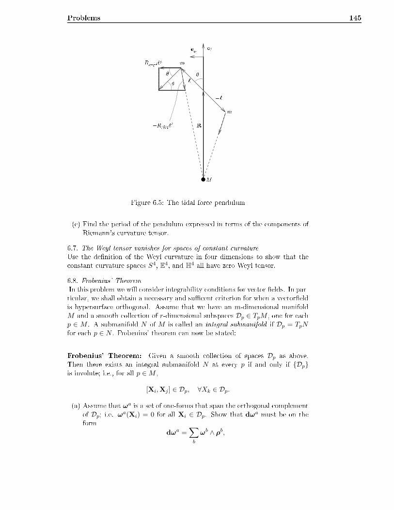
Problems 145

Rrtrt`rRtt` m ` ` m

erR

e

MFigure 6.5: The tidal for e pendulum( ) Find the period of the pendulum expressed in terms of the omponents ofRiemann's urvature tensor.6.7. The Weyl tensor vanishes for spa es of onstant urvatureUse the denition of the Weyl urvature in four dimensions to show that the onstant urvature spa es S4, E4, and H4 all have zero Weyl tensor.6.8. Frobenius' TheoremIn this problem we will onsider integrability onditions for ve tor elds. In par-ti ular, we shall obtain a ne essary and su ent riterion for when a ve toreldis hypersurfa e orthogonal. Assume that we have an m-dimensional manifoldM and a smooth olle tion of r-dimensional subspa es Dp ∈ TpM , one for ea hp ∈ M . A submanifold N of M is alled an integral submanifold if Dp = TpNfor ea h p ∈ N . Frobenius' theorem an now be stated:Frobenius' Theorem: Given a smooth olle tion of spa es Dp as above.Then there exists an integral submanifold N at every p if and only if Dpis involute; i.e., for all p ∈M ,

[Xi,Xj ] ∈ Dp, ∀Xk ∈ Dp.(a) Assume that ωa is a set of one-forms that span the orthogonal omplementof Dp; i.e. ωa(Xi) = 0 for all Xi ∈ Dp. Show that dωa must be on theformdωa =

∑

b

ωb ∧ ρb,

146 Chapter 6. Curvaturewhere ea h ρb is in T ∗pM . (Hint: Show rst that XµY ν∇[µω

aν] = 0 for all

Xµ, Y ν ∈ TpN .)(b) In parti ular, this means if M is an m-dimensional manifold and ξµ is a ovariant ve tor eld, then ξµ is hypersurfa e orthogonal to some (m −1)-dimensional submanifold if and only if ∇[µξν] = ξ[µρν]. Show that asu ent ondition for ξµ to be hypersurfa e orthogonal is

ξ[µ∇νξσ] = 0. (6.80)

Chapter 7Einstein's Field Equations7.1 Energy-momentum onservation7.1.1 Newtonian uidEnergy-momentum onservation for a Newtonian uid in terms of the divergen eof the energy momentum tensor an be shown as follows. The total derivativeof a velo ity eld isD~v

Dt≡ ∂~v

∂t+ (~v · ~∇)~v (7.1)

∂~v∂t is the lo al derivative whi h gives the hange in ~v as a fun tion of timeat a given point in spa e. (~v · ~∇)~v is alled the onve tive derivative of ~v. Itrepresents the hange of ~v for a moving uid parti le due to the inhomogeneityof the uid velo ity eld. In omponent notation the above be ome

Dvi

Dt≡ ∂vi

∂t+ vj

∂vi

∂xj(7.2)The ontinuity equation

∂ρ

∂t+ ∇ · (ρ~v) = 0 or ∂ρ

∂t+∂(ρvi)

∂xi= 0 (7.3)Euler's equation of motion (ignoring gravity)

ρD~v

Dt= −~∇p or ρ

(∂vi

∂t+ vj

∂vi

∂xj

)= − ∂p

∂xi(7.4)The energy momentum tensor is a symmetri tensor of rank 2 thatdes ribes material hara teristi s.

T µν =

T 00 T 01 T 02 T 03

T 10 T 11 T 12 T 13

T 20 T 21 T 22 T 23

T 30 T 31 T 32 T 33

(7.5)c ≡ 1147

148 Chapter 7. Einstein's Field EquationsT 00 represents energy density.T i0 represents momentum density.T ii represents pressure (T ii > 0).T ii represents stress (T ii < 0).T ij represents shear for es (i 6= j).Example 7.1.1 (Energy momentum tensor for a Newtonian uid)

T 00 = ρ T i0 = ρvi

T ij = ρvivj + pδij(7.6)where p is pressure, assumed isotropi here. We hoose a lo ally Cartesian oordinatesystem in an inertial frame su h that the ovariant derivatives are redu ed to partialderivatives. The divergen e of the momentum energy tensor, T µν;ν has 4 omponents,one for ea h value of µ.The zeroth omponent is

T 0ν;ν = T 0ν

,ν = T 00,0 + T 0i

,i

=∂ρ

∂t+∂(ρvi)

∂xi

(7.7)whi h by omparison to Newtonian hydrodynami s implies that T 0ν;ν = 0 is the ontinuity equation. This equation represents the onservation of energy.The ith omponent of the divergen e is

T iν,ν = T i0,0 + T ij,j

=∂(ρvi)

∂t+∂(ρvivj + pδij)

∂xj

= ρ∂vi

∂t+ vi

∂ρ

∂t+ vi

∂ρvj

∂xj+ ρvj

∂vi

∂xj+∂p

∂xi

(7.8)now, a ording to the ontinuity equation∂(ρvi)

∂xi= −∂ρ

∂t

⇒ T iν,ν = ρ∂vi

∂t+ vi

∂ρ

∂t− vi

∂ρ

∂t+ ρvj

∂vi

∂xj+∂p

∂xi

= ρDvi

Dt+∂p

∂xi

∴ T iν;ν = 0 ⇒ ρDvi

Dt= − ∂p

∂xi

(7.9)whi h is Euler's equation of motion. It expresses the onservation of momentum.

7.2 Einstein's urvature tensor 149The equations T µν;ν = 0 are general expressions for energy and momentum onservation.7.1.2 Perfe t uidsA perfe t uid is a uid with no vis osity and is given by the energy-momentumtensorTµν = (ρ+

p

c2)uµuν + pgµν (7.10)where ρ and p are the mass density and the stress, respe tively, measured in theuids rest frame, uµ are the omponents of the 4-velo ity of the uid.In a omoving orthonormal basis the omponents of the 4-velo ity are uµ =

(c, 0, 0, 0). Then the energy-momentum tensor is given byTµν =

ρc2 0 0 00 p 0 00 0 p 00 0 0 p

(7.11)where p > 0 is pressure and p < 0 is tension.There are three dierent types of perfe t uids that are useful.1. dust or non-relativisti gas is given by p = 0 and the energy-momemtumtensor Tµν = ρuµuν .2. radiation or ultra-relativisti gas is given by a tra eless energy-momemtumtensor, i.e. T µµ = 0. It follows that p = 13ρc

2.3. va uum energy: If we assume that no velo ity an be measured relativelyto va uum, then all the omponents of the energy-momentum tensor mustbe Lorentz-invariant. It follows that Tµν ∝ gµν . If va uum is dened as aperfe t uid we get p = −ρc2 so that Tµν = pgµν = −ρc2gµν .7.2 Einstein's urvature tensorThe eld equations are assumed to have the form:spa e-time urvature ∝ momentum-energy tensorAlso, it is demanded that energy and momentum onservation should follow asa onsequen e of the eld equation. This puts the following onstraints on the urvature tensor: It must be a symmetri , divergen e free tensor of rank 2.Bian hi's 2nd identity:Rµναβ;σ +Rµνσα;β +Rµνβσ;α = 0 (7.12) ontra tion of µ and α ⇒Rµνµβ;σ −Rµνµσ;β +Rµνβσ;µ = 0

R νβ;σ −R νσ;β +Rµνβσ;µ = 0(7.13)

150 Chapter 7. Einstein's Field Equationsfurther ontra tion of ν and σ givesRσβ;σ −Rσσ;β +Rσµσβ;µ = 0

Rσβ;σ −R ;β +Rσβ;σ = 0

∴ 2Rσβ;σ = R ;β

(7.14)Thus, we have al ulated the divergen e of the Ri i tensor,Rσβ;σ =

1

2R ;β (7.15)Now we use this expression together with the fa t that the metri tensor is o-variant and divergen e free to onstru t a new divergen e free urvature tensor.

Rσβ;σ −1

2R ;β = 0 (7.16)Keeping in mind that (gσβR);σ = gσβR;σ we multiply (7.16) by gβα to get

gβαRσβ;σ − gβα

1

2R ;β = 0

(gβαR

σβ

)

;σ− 1

2

(gβαR

)

;β= 0

(7.17)inter hanging σ and β in the rst term of the last equation:(gσαR

βσ

)

;β− 1

2

(gβαR

)

;β= 0

⇒(Rβα − 1

2δβαR

)

;β

= 0(7.18)sin e gσαRβσ=δσαRβσ=Rβα. So that Rβα − 1

2δβαR is the divergen e free urvaturetensor desired.This tensor is alled the Einstein tensor and its ovariant omponents aredenoted by Eαβ . That is

Eαβ = R αβ −1

2g αβR (7.19)NOTE THAT: Eµν;ν = 0 → 4 equations, giving only 6 equations from E µν ,whi h se ures a free hoi e of oordinate system.7.3 Einstein's eld equationsEinstein's eld equations:

Eµν = κTµν (7.20)

7.3 Einstein's eld equations 151orRµν −

1

2gµνR = κTµν (7.21)Contra tion gives:

R− 1

24R = κT , where T ≡ T µµ

R = −κT(7.22)

Rµν =1

2gµν(−κT ) + κTµν , (7.23)Thus the eld equations may be written in the form

Rµν = κ(Tµν −1

2gµνT ) (7.24)In the Newtonian limit the metri may be written

ds2 = −(

1 +2φ

c2

)c2dt2 + (1 + hii)(dx

2 + dy2 + dz2) (7.25)where the Newtonian potential |φ| ≪ c2, and hii is a perturbation of the metri satisfying |hii| << 1. We also have T00 ≫ Tkk and T ≈ −T00. Then the00- omponent of the eld equations be omes

R00 ≈ κ

2T00 (7.26)Furthermore we have

R00 = Rµ0µ0 = Ri0i0

= Γi00,i − Γi0i,0

=∂Γk00∂xk

=1

c2∇2φ (7.27)Sin e T00 ≈ ρc2 eq.(7.26) an be written ∇2φ = 1

2κc4ρ. Comparing this equationwith the Newtonian law of gravitation on lo al form: ∇2φ = 4πGρ, we see that

κ = 8πGc4

.In lassi al va uum we have : Tµν = 0, whi h givesEµν = 0 or Rµν = 0 . (7.28)These are the va uum eld equations. Note that Rµν = 0 does not imply

Rµναβ = 0.

152 Chapter 7. Einstein's Field EquationsDigression 7.3.1 (Lagrange (variation prin iple))It was shown by Hilbert that the eld equations may be dedu ed from a variationprin iple with a tion ∫R√−gd4x , (7.29)where R√−g is the Lagrange density. One may also in lude a so- alled osmologi al onstant Λ: ∫

(R + 2Λ)√−gd4x (7.30)The eld equations with osmologi al onstant are

Rµν −1

2gµνR+ Λgµν = κTµν (7.31)7.4 The geodesi postulate as a onsequen e of theeld equationsThe prin iple that free parti les follow geodesi urves has been alled thegeodesi postulate. We shall now show that the geodesi postulate followsas a onsequen e of the eld equations.Consider a system of free parti les in urved spa e-time. This system anbe regarded as a pressure-free gas. Su h a gas is alled dust. It is des ribed byan energy-momentum tensorT µν = ρuµuν (7.32)where ρ is the rest density of the dust as measured by an observer at rest in thedust and uµ are the omponents of the four-velo ity of the dust parti les.Einstein's eld equations as applied to spa e-time lled with dust, take theform

Rµν − 1

2gµνR = κρuµuν (7.33)Be ause the divergen e of the left hand side is zero, the divergen e of the righthand side must be zero, too

(ρuµuν);ν = 0 (7.34)or(ρuνuµ);ν = 0 (7.35)we now regard the quantity in the parenthesis as a produ t of ρuν and uµ. Bythe rule for dierentiating a produ t we get

(ρuν);νuµ + ρuνuµ;ν = 0 (7.36)

Problems 153Sin e the four-velo ity of any obje t has a magnitude equal to the velo ity oflight we haveuµu

µ = −c2 (7.37)Dierentiation gives(uµu

µ);ν = 0 (7.38)Using, again, the rule for dierentiating a produ t, we getuµ;νu

µ + uµuµ;ν = 0 (7.39)From the rule for raising an index and the freedom of hanging a summationindex from α to µ, say, we get

u µ;νuµ = uµuµ;ν = gµαuαuµ;ν = uαg

µαuµ;ν = uαuα;ν = uµu

µ;ν (7.40)Thus the two terms of eq.(7.39) are equal. It follows that ea h of them are equalto zero. So we have

uµuµ;ν = 0 (7.41)Multiplying eq.(7.36) by uµ, we get

(ρuν);νuµuµ + ρuνuµu

µ;ν = 0 (7.42)Using eq.(7.37) in the rst term, and eq.(7.41) in the last term, whi h thenvanishes, we get

(ρuν);ν = 0 (7.43)Thus the rst term in eq.(7.36) vanishes and we getρuνuµ;ν = 0 (7.44)Sin e ρ 6= 0 we must haveuνuµ;ν = 0 (7.45)This is just the geodesi equation. Con lusion: It follows from Einstein'seld equations that free parti les move along paths orresponding to geodesi urves of spa e-time.Problems7.1. Lorentz transformation of a perfe t uidConsider a homogeneous perfe t uid. In the rest frame of the uid the equationof state is p = wρ (with c = 1), and the energy-momentum tensor has the form

Tµν = ρdiag(1, w,w,w). (7.46)

154 Chapter 7. Einstein's Field Equations(a) Make a Lorentz transformation in the 1−dire tion with velo ity v and showthat the transformed energy-momentum tensor has the formTµ′ν′ = ρ

γ2(1 + v2w) γ2v(1 + w) 0 0γ2v(1 + w) γ2(v2 + w) 0 0

0 0 w 00 0 0 w

, γ =1√

1 − v2. (7.47)(b) The weak energy ondition requires that the energy-density is positive.What restri tion does this put on w?( ) Whi h value of w makes the omponents of the energy-momentum tensorLorentz invariant?7.2. Geodesi equation and onstants of motionShow that the ovariant omponents of the geodesi equation have the form

uµ =1

2gαβ,µu

αuβ.What does this equation tell about onstants of motion for free parti les?7.3. The ele tromagneti energy-momentum tensorConsider a general energy-momentum tensor Tµν and a time-like ve tor uµ. We an always de ompose Tµν as follows:Tµν = ρuµuν + phµν + 2u(µqν) + πµν , (7.48)where ρ is the energy density; p is the isotropi pressure; qµ is the energy ux;

πµν is the anisotropi stress tensor; and hµν = gµν +uµuν is the 3-metri tensoron the hypersurfa es orthogonal to uµ. These fulll the following relations:uµqµ = uµπµν = uµhµν = πµµ = 0, πνµ = πµν .(a) Show thatρ = Tµνu

µuν , p =1

3Tµνh

µν ,

qν = −uµhρνTµρ, πµν = Tρσ

(hρµh

σν −

1

3hρσhµν

). (7.49)(b) Consider the ele tromagneti eld tensorin an orthonormal basis et, ei.Assume that uµ is aligned with the time-like basis ve tor et. Use theele tromagneti energy-momentum tensor to show that

ρ = 3p =1

2(EkEk +BkBk),

qi = −εijkEjBk,

πij = −EiEj −BiBj +1

3δij(E

kEk +BkBk). (7.50)What is the physi al interpretation of qi?

Problems 1557.4. Lorentz-invariant radiationConsider a region lled with photons of all frequen ies and moving in all di-re tions. Let n(ν, e) be the number of photons per unit volume, per frequen yinterval, and per unit solid angle moving in the dire tion e, as referred to anorthonormal basis Σ. Let primed quantities be measured in a basis Σ′ movingwith a velo ity v relative to Σ. A omoving volume element dV has a velo ityu in Σ. The orresponding rest volume is dV0.The quantity n(ν, e)dV dνdΩ represents the number of photons o upying avolume dV , with frequen ies between ν and ν+ dν, and moving with dire tionswithin a solid angle dΩ = sin θdθdφ. It is an invariant quantity. Hen e,

n(ν, e)dV dνdΩ = n′(ν ′, e′)dV ′dν ′dΩ′.(a) Use that dV0 is invariant to show that dV ′ = γ−1u′ γudV where γu′ = (1 −

|u′|2/c2)−1/2 and γu = (1 − |u|2/c2)−1/2.(b) Choose the x′- and x-axes to be dire ted along v (so that v = vex) anduse the transformation formulae of the velo ity omponents,u′x =

ux − v

1 − uxvc2, u′y =

uy

γv(1 − uxv

c2

) , γv =

(1 − v2

c2

)− 12

,to show thatγu′ = γuγv

(1 − u · v

c2

)−1;and hen e that

dV ′ = γ−1v

(1 − u · v

c2

)−1dV.( ) Let θ be the angle between the transformation velo ity v and the velo ity

u of the volume. Sin e the volume is omoving with photons moving inthe u-dire tion, we now set |u| = c. Show that this leads to dV ′ = κ−1dV ,where κ = γv[1 − (v/c) cos θ].(d) Use the relativisti equations for the Doppler ee t and abberation (seeproblem 2.9), and show that the transformation equations for the dieren-tials of frequen y and solid angle aredν ′ = κdν, dΩ′ = κ−2dΩ.(e) Dedu e that n′(ν ′, e′) = κ2n(ν, e) and use the transformation equation forthe frequen y to show that n(ν, e)/ν2 is a Lorentz-invariant quantity.(f) Sin e ν is not Lorentz invariant it follows that n(ν, e)/ν2 must be inde-pendent of ν. Use this, together with the fa t that the energy of a photonis given by hν, to nd how the energy-density per frequen y interval andsolid angle of a Lorentz-invariant radiation depends upon the frequen y.

Chapter 8The S hwarzs hild spa etime8.1 S hwarzs hild's exterior solutionThis is a solution of the va uum eld equations Eµν = 0 for a stati spheri allysymmetri spa etime. One an then hoose the following form of the line element(employing units so that =1),ds2 = −e2α(r)dt2 + e2β(r)dr2 + r2dΩ2

dΩ2 = dθ2 + sin2 θdφ2(8.1)These oordinates are hosen so that the area of a sphere with radius r is 4πr2.Physi al distan e in radial dire tion, orresponding to a oordinate distan e

dr, is dlr =√grrdr = eβ(r)dr.Here follows a stepwise algorithm to determine the omponents of the Ein-stein tensor by using the Cartan formalism:1. Using orthonormal basis we nd

ωt = eα(r)dt , ωr = eβ(r)dr , ωθ = rdθ , ωφ = r sin θdφ (8.2)2. Computing the onne tion forms by applying Cartan's 1. stru ture equa-tionsdωµ = −Ωµν ∧ ων (8.3)

dωt = eαα′dr ∧ dt= eαα′e−βωr ∧ e−αωt

= −e−βα′ωt ∧ ωr

= −Ωtr ∧ ωr

(8.4)∴ Ωt

r = e−βα′ωt + f1ωr (8.5)156

8.1 S hwarzs hild's exterior solution 1573. To determine the f-fun tions we apply the anti-symmetryΩ µν = −Ω νµ (8.6)This gives (the non-zero onne tion forms):

Ωrφ

= −Ωφr = −1

re−βωφ

Ωθφ

= −Ωφ

θ= −1

rcot θωφ

Ωtr = +Ωr

t= e−βα′ωt

Ωrθ

= −Ωθr = −1

re−βωθ

(8.7)4. We then pro eed to determine the urvature forms by applying Cartan's2nd stru ture equations

Rµν = dΩµν + Ωµα ∧ Ωαν (8.8)whi h gives:

Rtr = −e−2β(α′′ + α′2 − α′β′)ωt ∧ ωr

Rtθ

= −1

re−2βα′ωt ∧ ωθ

Rtφ

= −1

re−2βα′ωt ∧ ωφ

Rrθ

=1

re−2ββ′ωr ∧ ωθ

Rrφ

=1

re−2ββ′ωr ∧ ωφ

Rθφ

=1

r2(1 − e−2β)ωθ ∧ ωφ

(8.9)5. By applying the following relation

Rµν =1

2Rµναβ

ωα ∧ ωβ (8.10)we nd the omponents of Riemann's urvature tensor.6. Contra tion gives the omponents of Ri i's urvature tensorRµν ≡ Rαµαν (8.11)7. A new ontra tion gives Ri i's urvature s alarR ≡ Rµµ (8.12)

158 Chapter 8. The S hwarzs hild spa etime8. The omponents of the Einstein tensor an then be foundEµν = Rµν −

1

2ηµνR , (8.13)where ηµν = diag(−1, 1, 1, 1). We then have:

Ett =2

re−2ββ′ +

1

r2(1 − e−2β)

Err =2

re−2βα′ − 1

r2(1 − e−2β)

Eθθ = Eφφ = e−2β(α′′ + α′2 − α′β′ +α′

r− β′

r)

(8.14)We want to solve the equations Eµν = 0. We get only 2 independentequations, and hoose to solve those:Ett = 0 and Err = 0 (8.15)By adding the 2 equations we get:

Ett + Err = 0

⇒ 2

re−2β(β′ + α′) = 0

⇒ (α+ β)′ = 0 ⇒ α+ β = K1 ( onst) (8.16)We now have:ds2 = −e2αdt2 + e2βdr2 + r2dΩ2 (8.17)By hoosing a suitable oordinate time, we an a hieve

K1 = 0 ⇒ α = −βSin e we have ds2 = −e2αdt2 + e−2αdr2 + r2dΩ2, this means that grr =− 1gtt. We still have to solve one more equation to get the omplete solution,and hoose the equation Ett = 0, whi h gives

2

re−2ββ′ +

1

r2(1 − e−2β) = 0This equation an be written:

1

r2d

dr[r(1 − e−2β)] = 0

∴ r(1 − e−2β) = K2 ( onst) (8.18)If we hoose K2 = 0 we get β = 0 giving α = 0 andds2 = −dt2 + dr2 + r2dΩ2 , (8.19)

8.1 S hwarzs hild's exterior solution 159whi h is the Minkowski spa e-time des ribed in spheri al oordinates. Ingeneral, K2 6= 0 and 1 − e−2β = K2r ≡ K

r , givinge2α = e−2β = 1 − K

randds2 = −(1 − K

r)dt2 +

dr2

1 − Kr

+ r2dΩ2 (8.20)We an nd K by going to the Newtonian limit. We al ulate the gravita-tional a eleration ( that is, the a eleration of a free parti le instantanously atrest ) in the limit of a weak eld of a parti le at a distan e r from a spheri almass M . Newtonian:g =

d2r

dt2= −GM

r2(8.21)We anti ipate that r >> K. Then the proper time τ of a parti le will beapproximately equal to the oordinate time, sin e dτ =

√1 − K

r dtThe a eleration of a parti le in 3-spa e, is given by the geodesi equation:d2xµ

dτ2+ Γµαβu

αuβ = 0

uα =dxα

dτ

(8.22)For a parti le instantanously at rest in a weak eld, we have dτ ≈ dt. Usinguµ = (1, 0, 0, 0), we get:

g =d2r

dt2= −Γrtt (8.23)This equation gives a physi al interpretation of Γrtt as the gravitational a eler-ation. This is a mathemati al way to express the prin iple of equivalen e: Thegravitational a eleration an be transformed to 0, sin e the Christoel symbolsalways an be transformed to 0 lo ally, in a freely falling non-rotating frame,i.e. a lo al inertial frame.

Γrtt =1

2grα︸︷︷︸

1grα

(∂gαt∂t︸ ︷︷ ︸=0

+∂gαt∂t︸ ︷︷ ︸=0

−∂gtt∂xα

)

= − 1

2grr

∂gtt∂r

gtt = −(1 − K

r) , ∂gtt

∂r= −K

r2

g = −Γrtt = − K

2r2= −GM

r2gives K = 2GMor with : K =2GM

c2

(8.24)

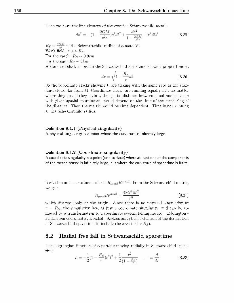
160 Chapter 8. The S hwarzs hild spa etimeThen we have the line element of the exterior S hwarzs hild metri :ds2 = −(1 − 2GM

c2r)c2dt2 +

dr2

1 − 2GMc2r

+ r2dΩ2 (8.25)RS ≡ 2GM

c2is the S hwarzs hild radius of a mass M.Weak eld: r >> RS .For the earth: RS ∼ 0.9cmFor the sun: RS ∼ 3kmA standard lo k at rest in the S hwarzs hild spa etime shows a proper time τ :

dτ =

√1 − RS

rdt (8.26)So the oordinate lo ks showing t, are ti king with the same rate as the stan-dard lo ks far from M. Coordinate lo ks are running equally fast no matterwhere they are. If they hadn't, the spatial distan e between simultanous eventswith given spatial oordinates, would depend on the time of the measuring ofthe distan e. Then the metri would be time dependent. Time is not runningat the S hwarzs hild radius.Denition 8.1.1 (Physi al singularity)A physi al singularity is a point where the urvature is innitely large.Denition 8.1.2 (Coordinate singularity)A oordinate singularity is a point (or a surfa e) where at least one of the omponentsof the metri tensor is innitely large, but where the urvature of spa etime is nite.Krets hmann's urvature s alar is RµναβRµναβ . From the S hwarzs hild metri ,we get:

RµναβRµναβ =

48G2M2

r8(8.27)whi h diverges only at the origin. Sin e there is no physi al singularity at

r = RS , the singularity here is just a oordinate singularity, and an be re-moved by a transformation to a oordinate system falling inward. (Eddington -Finkelstein oordinates, Kruskal - Szekers analyti al extension of the des riptionof S hwarzs hild spa etime to in lude the area inside RS).8.2 Radial free fall in S hwarzs hild spa etimeThe Lagrangian fun tion of a parti le moving radially in S hwarzs hild spa e-timeL = −1

2(1 − RS

r)c2 t2 +

1

2

r2

(1 − RS

r ), · ≡ d

dτ(8.28)

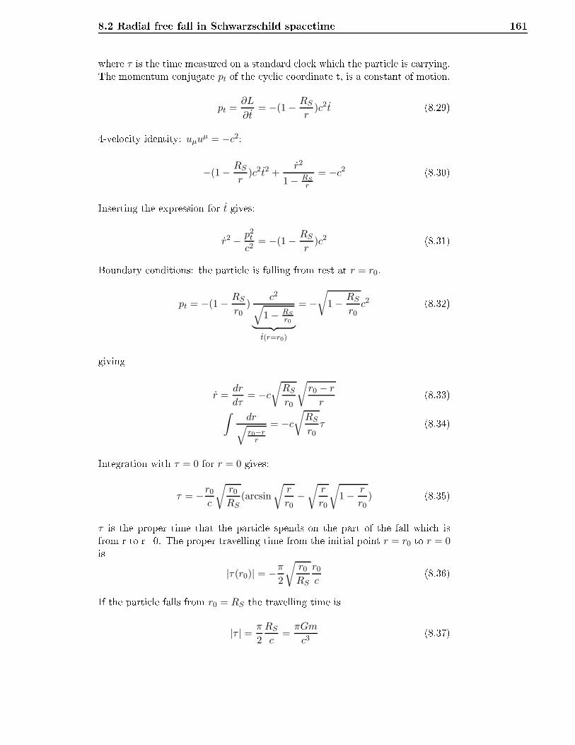
8.2 Radial free fall in S hwarzs hild spa etime 161where τ is the time measured on a standard lo k whi h the parti le is arrying.The momentum onjugate pt of the y li oordinate t, is a onstant of motion.pt =

∂L

∂t= −(1 − RS

r)c2t (8.29)4-velo ity identity: uµuµ = −c2:

−(1 − RSr

)c2t2 +r2

1 − RS

r

= −c2 (8.30)Inserting the expression for t gives:r2 − p2

t

c2= −(1 − RS

r)c2 (8.31)Boundary onditions: the parti le is falling from rest at r = r0.

pt = −(1 − RSr0

)c2√

1 − RS

r0︸ ︷︷ ︸t(r=r0)

= −√

1 − RSr0c2 (8.32)

givingr =

dr

dτ= −c

√RSr0

√r0 − r

r(8.33)

∫dr√r0−rr

= −c√RSr0τ (8.34)Integration with τ = 0 for r = 0 gives:

τ = −r0c

√r0RS

(arcsin

√r

r0−√

r

r0

√1 − r

r0) (8.35)

τ is the proper time that the parti le spends on the part of the fall whi h isfrom r to r=0. The proper travelling time from the initial point r = r0 to r = 0is|τ(r0)| = −π

2

√r0RS

r0c

(8.36)If the parti le falls from r0 = RS the travelling time is|τ | =

π

2

RSc

=πGm

c3(8.37)

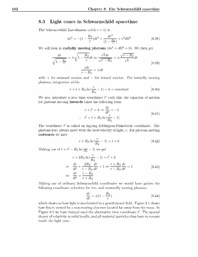
162 Chapter 8. The S hwarzs hild spa etime8.3 Light ones in S hwarzs hild spa etimeThe S hwarzs hild line-element (with c = 1) isds2 = −(1 − RS

r)dt2 +

dr2

(1 − RS

r )+ r2dΩ2 (8.38)We will look at radially moving photons (ds2 = dΩ2 = 0). We then get

dr√1 − RS

r

= ±√

1 − RSrdt⇔ r

12 dr√r −RS

= ±√r −RS

r12

dt

rdr

r −RS= ±dt

(8.39)with + for outward motion and − for inward motion. For inwardly movingphotons, integration yieldsr + t+RS ln | r

RS− 1| = k = constant (8.40)We now introdu e a new time oordinate t′ su h that the equation of motionfor photons moving inwards takes the following form

r + t′ = k ⇒ dr

dt′= −1

∴ t′ = t+RS ln | rRS

− 1|(8.41)The oordinate t′ is alled an ingoing Eddington-Finkelstein oordinate. Thephotons here always move with the lo al velo ity of light, c. For photons movingoutwards we have

r +RS ln | rRS

− 1| = t+ k (8.42)Making use of t = t′ −RS ln | rRS− 1| we get

r + 2RS ln | rRS

− 1| = t′ + k

⇒ dr

dt′+

2RSr −RS

dr

dt′= 1 ⇔ r +RS

r −RS

dr

dt′= 1

⇔ dr

dt′=r −RSr +RS

(8.43)Making use of ordinary S hwarzs hild oordinates we would have gotten thefollowing oordinate velo ities for inn- and outwardly moving photons:dr

dt= ±(1 − RS

r) (8.44)whi h shows us how light is de elerated in a gravitational eld. Figure 8.1 showshow this is viewed by a non-moving observer lo ated far away from the mass. InFigure 8.2 we have instead used the alternative time oordinate t′. The spe ialtheory of relativity is valid lo ally, and all material parti les thus have to remaininside the light one.

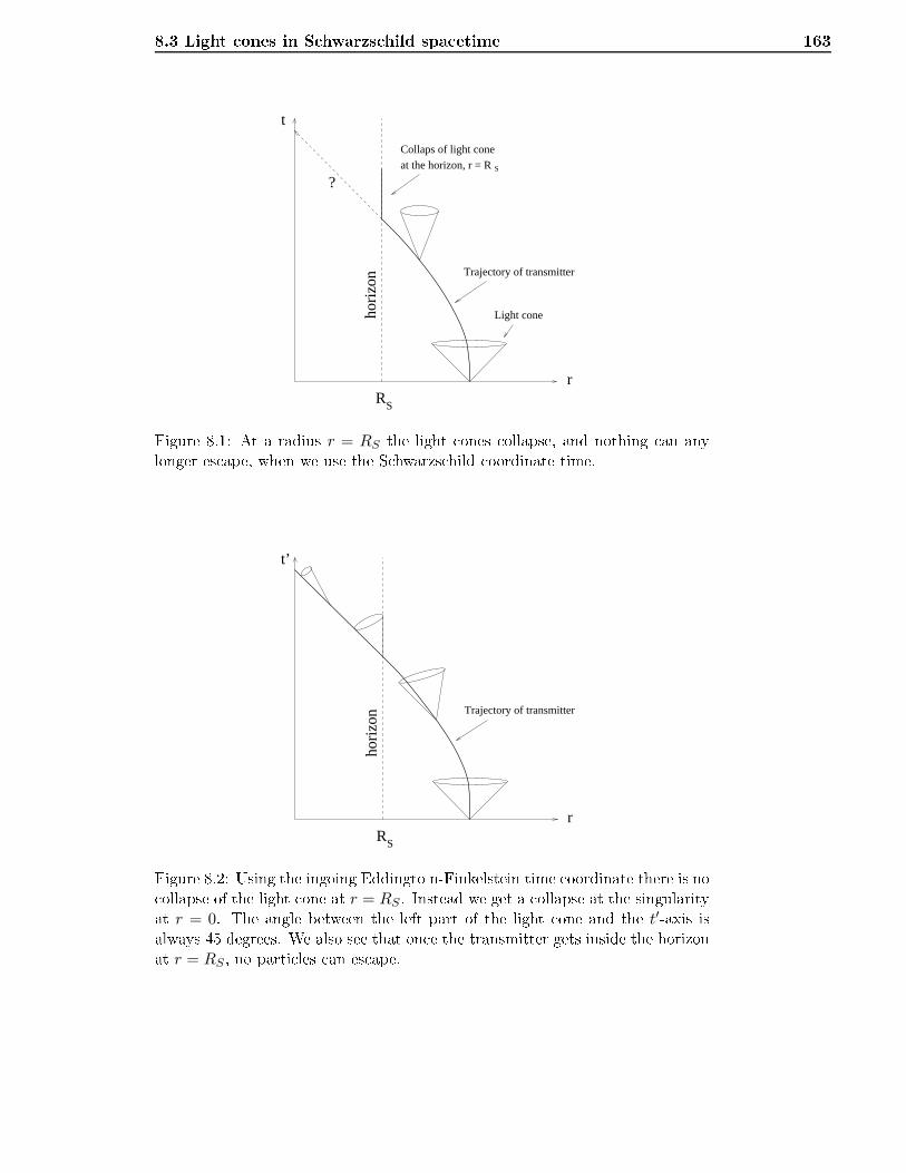
8.3 Light ones in S hwarzs hild spa etime 163S

hori

zon

RS

r

Trajectory of transmitter

t

?

Light cone

Collaps of light cone

at the horizon, r = R

Figure 8.1: At a radius r = RS the light ones ollapse, and nothing an anylonger es ape, when we use the S hwarzs hild oordinate time.t’

hori

zon

RS

r

Trajectory of transmitter

Figure 8.2: Using the ingoing Eddingto n-Finkelstein time oordinate there is no ollapse of the light one at r = RS . Instead we get a ollapse at the singularityat r = 0. The angle between the left part of the light one and the t′-axis isalways 45 degrees. We also see that on e the transmitter gets inside the horizonat r = RS , no parti les an es ape.

164 Chapter 8. The S hwarzs hild spa etime8.4 Analyti al extension of the S hwarzs hild oordi-natesThe S hwarzs hild oordinates are omoving with a stati referen e frame out-side a spheri al mass distribution. If the mass has ollapsed to a bla k holethere exist a horizon at the S hwarzs hild radius. As we have seen in se tion8.3 there do not exist stati observers at nite radii inside the horizon. Hen e,the S hwarzs hild oordinates are well dened only outside the horizon.Also the rr- omponent of the metri tensor has a oordinate singularity atthe S hwarzs hild radius. The urvature of spa etime is nite here.Kruskal and Szekeres have introdu ed new oordinates that are well denedinside as well as outside the S hwarzs hild radius, and with the property thatthe metri tensor is non-singular for all r > 0.In order to arrive at these oordinates we start by onsidering a photonmoving radially inwards. From eq. (8.40) we then havet = −r −RS ln

∣∣∣∣r

RS− 1

∣∣∣∣+ v (8.45)where v is a onstant along the world line of the photon. We introdu e a newradial oordinater∗ ≡ r +RS ln

∣∣∣∣r

RS− 1

∣∣∣∣ (8.46)Then the equation of the worldline of the photon takes the formt+ r∗ = v (8.47)The value of the onstant v does only depend upon the point of time when thephoton was emitted. We may therefore use v as a new time oordinate.For an outgoing photon we get in the same wayt− r∗ = u (8.48)where u is a onstant of integration, whi h may be used as a new time oordinatefor outgoing photons. The oordinates u and v are the generalization of the light one oordinates of Minkowski spa etime to the S hwarz hild spa etime.From eqs. (8.47) and (8.48) we get

dt =1

2(dv + du) (8.49)

dr∗ =1

2(dv − du) (8.50)and from eq. (8.46)

dr =

(1 − Rs

r

)dr∗ (8.51)Inserting these dierentials into eq. (8.38) we arrive at a new form of theS hwarzs hild line-element,

ds2 = −(

1 − Rsr

)du dv + r2dΩ2 (8.52)

8.4 Analyti al extension of the S hwarzs hild oordinates 165The metri is still not well behaved at the horizon. Introdu ing the oordinatesU = −e−

u2Rs (8.53)

V = ev

2Rs (8.54)givesUV = −e

v−u2Rs = −e

r∗

Rs = −∣∣∣∣Rsr

− 1

∣∣∣∣ er

Rs (8.55)anddu dv = −4R 2

s

dUdV

UV(8.56)The line-element (8.52) then takes the form

ds2 = −4R 3s

re−

rRs dUdV + r2dΩ2 (8.57)This is the rst form of the Kruskal-Szekeres line-element. Here is no oordinatesingularity, only a physi al singularity at r = 0.We may furthermore introdu e two new oordinates

T =1

2(V + U) =

∣∣∣∣r

Rs− 1

∣∣∣∣

12

er

2Rs sinht

2Rs(8.58)

Z =1

2(V − U) =

∣∣∣∣r

Rs− 1

∣∣∣∣

12

er

2Rs cosht

2Rs(8.59)Hen e

V = T + Z (8.60)U = T − Z (8.61)giving

dUdV = dT 2 − dZ2 (8.62)Inserting this into eq. (8.57) we arrive at the se ond form of the Kruskal-Szekeresline-elementds2 = −4R 3

s

re−

rRs

(dT 2 − dZ2

)+ r2dΩ2 (8.63)The inverse transformations of eqs. (8.58) and (8.59) is

∣∣∣∣r

Rs− 1

∣∣∣∣ er

Rs = Z2 − T 2 (8.64)tanh

t

2Rs=T

Z(8.65)Note from eq. (8.63) that with the Kruskal-Szekeres oordinates T and Zthe equation of the radial null geodesi s has the same form as in at spa etime

Z = ±T + onstant (8.66)

166 Chapter 8. The S hwarzs hild spa etime8.5 Embedding of the S hwarzs hild metri We will now look at a stati , spheri ally symmetri spa e. A urved simultaneityplane (dt = 0) through the equatorial plane (dθ = 0) has the line elementds2 = grrdr

2 + r2dφ2 (8.67)with a radial oordinate su h that a ir le with radius r has a ir umferen e oflength 2πr.We now embed this surfa e in a at 3-dimensional spa e with ylinder o-ordinates (z, r, φ) and line elementds2 = dz2 + dr2 + r2dφ2 (8.68)The surfa e des ribed by the line element in (8.67) has the equation z = z(r).The line element in (8.68) is therefore written as

ds2 = [1 + (dz

dr)2]dr2 + r2dφ2 (8.69)Demanding that (8.69) is in agreement with (8.67) we get

grr = 1 + (dz

dr)2 ⇔ dz

dr= ±

√grr − 1 (8.70)Choosing the positive solution gives

dz =√grr − 1dr (8.71)In the S hwarzs hild spa etime we have

grr =1

1 − RS

r

(8.72)Making use of this we nd z:z =

∫ r

RS

dr√rRS

− 1=√

4RS(r −RS) (8.73)This is shown in Figure 8.3.8.6 De eleration of lightThe radial speed of light in S hwarzs hild oordinates found by putting ds2 =dΩ2 = 0 in eq. (8.38) is

c = 1 − RSr

(8.74)To measure this ee t one an look at how long it takes for light to get fromMer ury to the Earth. This is illustrated in Figure 8.4. The travel time from

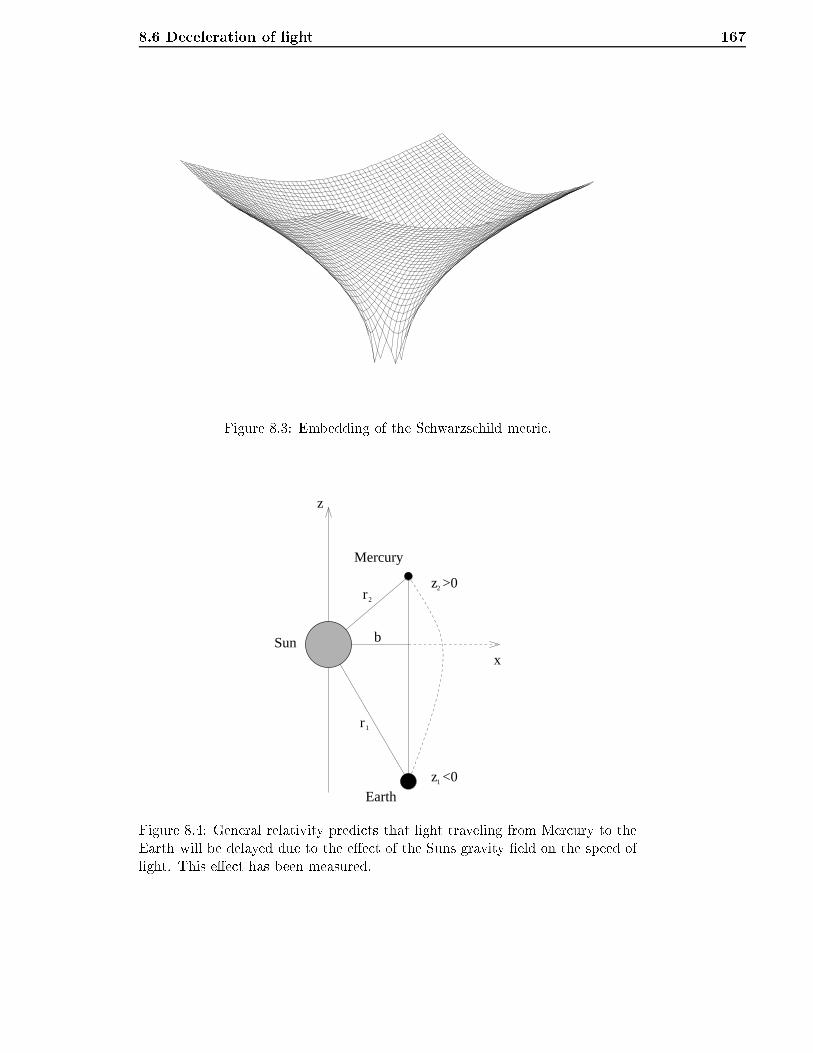
8.6 De eleration of light 167

Figure 8.3: Embedding of the S hwarzs hild metri .z

Sunx

b

Mercury

z1 <0

z2 >0r2

r1

EarthFigure 8.4: General relativity predi ts that light traveling from Mer ury to theEarth will be delayed due to the ee t of the Suns gravity eld on the speed oflight. This ee t has been measured.

168 Chapter 8. The S hwarzs hild spa etimez1 to z2 is

∆t =

∫ z2

z1

dz

1 − RS

r

≈∫ z2

z1

(1 +RSr

)dz =

∫ z2

z1

(1 +RS√b2 + z2

)dz

= z2 + |z1| +RS ln

√z22 + b2 + z2√z12 + b2 − |z1|

(8.75)where RS is the S hwarzs hild radius of the Sun.The de eleration is greatest when Earth and Mer ury (where the light isree ted) are on nearly opposite sides of the Sun. The impa t parameter b isthen small. A series expansion to the lowest order of b/z gives∆t = z2 + |z1| +RS ln

4|z1|z2b2

(8.76)The last term represents the extra traveling time due to the ee t of the Sunsgravity eld on the speed of light. The journey takes longer time:RS = the S hwarzs hild radius of the Sun ∼ 3km|z1|= the radius of Earth's orbit = 15 × 1010mz2 = the radius of Mer ury's orbit = 5.8 × 1010mb = R⊙ = 7 × 108mgive a delay of 1.1 × 10−4s. In addition to this one must also, of ourse, takeinto a ount among other things the ee ts of the urvature of spa etime nearthe Sun and atmospheri ee ts on Earth.8.7 Parti le traje tories in S hwarzs hild 3-spa e

L =1

2g µνX

µXν

= −1

2

(1 − Rs

r

)t2 +

12 r

2

1 − Rs

r

+1

2r2θ2 +

1

2r2 sin2 θφ2

(8.77)Sin e t is a y li oordinate−pt = −∂L

∂t=

(1 − Rs

r

)t = constant = E (8.78)where E is the parti le's energy as measured by an observer "far away" (r ≫ Rs).Also φ is a y li oordinate so that

pφ =∂L

∂φ= r2 sin2 θφ = constant (8.79)where pφ is the parti le's orbital angular momentum.

8.7 Parti le traje tories in S hwarzs hild 3-spa e 169Making use of the 4-velo ity identity ~U2 = g µνXµXν = −1 we transformthe above to get

−(

1 − Rsr

)t2 +

r2

1 − Rs

r

+ r2θ2 + r2 sin2 θφ2 = −1 (8.80)whi h on substitution for t = E1−Rs

r

and φ =pφ

r2 sin2 θbe omes

− E2

1 − Rs

r

+r2

1 − Rs

r

+ r2θ2 +p2φ

r2 sin2 θ= −1 (8.81)Now, refering ba k to the Lagrange equation

d

dτ

(∂L

∂Xµ

)− ∂L

∂Xµ= 0 (8.82)we get, for θ

(r2θ)• = r2 sin θ cos θφ2

=p2φ cos θ

r2 sin3 θ

(8.83)Multiplying this by r2θ we get(r2θ)(r2θ)• =

cos θθ

sin3 θp2φ (8.84)whi h, on integration, gives

(r2θ)2 = k −( pφ

sin θ

)2 (8.85)where k is the onstant of integration.Be ause of the spheri al geometry we are free to hoose a oordinate systemsu h that the parti le moves in the equatorial plane and along the equator at agiven time t = 0. That is θ = π2 and θ = 0 at time t = 0. This determines the onstant of integration and k = p2

φ su h that(r2θ)2 = p2

φ

(1 − 1

sin2 θ

) (8.86)The RHS is negative for all θ 6= π2 . It follows that the parti le annot deviatefrom its original (equatorial) traje tory. Also, sin e this parti ular hoi e oftraje tory was arbitrary we an on lude, quite generally, that any motion offree parti les in a spheri ally symmetri gravitational eld is planar motion.

170 Chapter 8. The S hwarzs hild spa etime8.7.1 Motion in the equatorial plane− E2

1 − Rs

r

+r2

1 − Rs

r

+p2φ

r2= −1 (8.87)that is

r2 = E2 −(

1 − Rsr

)(1 +

p2φ

r2

) (8.88)This orresponds to an energy equation with an ee tive potential V (r) givenbyV 2(r) =

(1 − Rs

r

)(

1 +p2φ

r2

)

r2 + V 2(r) = E2

⇒ V =

√

1 − rsr

+p2φ

r2−Rsp

2φ

r3

≅ 1 − 1

2

Rsr

+1

2

p2φ

r2

(8.89)Newtonian potential VN is dened by using the last expression in

VN = V − 1 ⇒ VN = −GMr

+p2φ

2r2(8.90)The possible traje tories of parti les in the S hwarzs hild 3-spa e are showns hemati ally in Figure 8.5 as fun tions of position and energy of the parti lein the Newtonian limit.To take into a ount the relativisti ee ts the above pi ture must be mod-ied. We introdu e dimensionless variables

X =r

GMand k =

pφGMm

(8.91)The potential V 2(r) now take the formV =

(1 − 2

X+k2

X2− 2k2

X3

)1/2 (8.92)For r equal to the S hwarzs hild radius (X = 2) we haveV (2) =

√1 − 1 +

k2

4− 2k2

8= 0 (8.93)For k2 < 12 parti les will fall in towards r = 0.

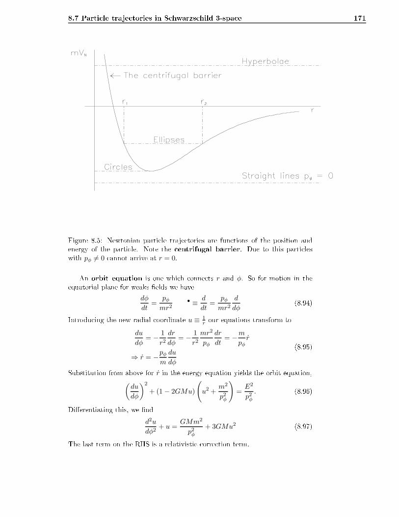
8.7 Parti le traje tories in S hwarzs hild 3-spa e 171

Figure 8.5: Newtonian parti le traje tories are fun tions of the position andenergy of the parti le. Note the entrifugal barrier. Due to this parti leswith pφ 6= 0 annot arrive at r = 0.An orbit equation is one whi h onne ts r and φ. So for motion in theequatorial plane for weaks elds we havedφ

dt=

pφmr2

• ≡ d

dt=

pφmr2

d

dφ(8.94)Introdu ing the new radial oordinate u ≡ 1

r our equations transform todu

dφ= − 1

r2dr

dφ= − 1

r2mr2

pφ

dr

dt= −m

pφr

⇒ r = −pφm

du

dφ

(8.95)Substitution from above for r in the energy equation yields the orbit equation,(du

dφ

)2

+ (1 − 2GMu)

(u2 +

m2

p2φ

)=E2

p2φ

. (8.96)Dierentiating this, we ndd2u

dφ2+ u =

GMm2

p2φ

+ 3GMu2 (8.97)The last term on the RHS is a relativisti orre tion term.

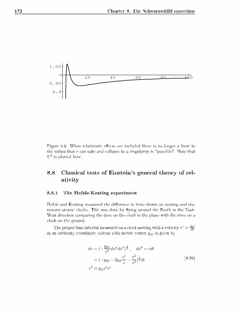
172 Chapter 8. The S hwarzs hild spa etime

20 40 60 80 100

0.9

0.95

1.05

Figure 8.6: When relativisti ee ts are in luded there is no longer a limit tothe values that r an take and ollapse to a singularity is "possible". Note thatV 2 is plotted here.8.8 Classi al tests of Einstein's general theory of rel-ativity8.8.1 The Hafele-Keating experimentHafele and Keating measured the dieren e in time shown on moving and sta-tionary atomi lo ks. This was done by ying around the Earth in the East-West dire tion omparing the time on the lo k in the plane with the time on a lo k on the ground.The proper time interval measured on a lo k moving with a velo ity vi = dxi

dtin an arbitrary oordinate system with metri tensor gµν is given bydτ = (−gµν

c2dxµdxν)

12 , dx0 = cdt

= (−g00 − 2gi0vi

c− v2

c2)

12 dt

v2 ≡ gijvivj

(8.98)

8.8 Classi al tests of Einstein's general theory of relativity 173For a diagonal metri tensor (gi0 = 0) we getdτ = (−g00 −

v2

c2)

12dt , v2 = gii(v

i)2 (8.99)We now look at an idealized situation where a plane ies at onstant altitudeand with onstant speed along the equator.dτ = (1 − RS

r− v2

c2)

12 dt , r = R+ h (8.100)To the lowest order in RS

r and v2

c2we get

dτ = (1 − RS2r

− 1

2

v2

c2)dt (8.101)The speed of the moving lo k is

v = (R+ h)Ω + u (8.102)where Ω is the angular velo ity of the Earth and u is the speed of the plane. Aseries expansion and use of this value for v gives∆τ = (1 − GM

Rc2− 1

2

R2Ω2

c2+gh

c2− 2RΩu+ u2

2c2)∆t , g =

GM

R2−RΩ2(8.103)

u > 0 when ying in the dire tion of the Earth's rotation, i.e. eastwards. For a lo k that is left on the airport (stationary, h = u = 0) we get∆τ0 = (1 − GM

Rc2− 1

2

R2Ω2

c2)∆t (8.104)To the lowest order the relative dieren e in travel time is

k =∆τ − ∆τ0

∆τ0∼= gh

c2− 2RΩu+ u2

2c2(8.105)Measurements:Travel time: ∆τ0 = 1.2 × 105s (a little over 24h)Traveling eastwards: ke = −1.0 × 10−12Traveling westwards: kw = 2.1 × 10−12

(∆τ − ∆τ0)e = −1.2 × 10−7s ≈ −120ns(∆τ − ∆τ0)w = 2.5 × 10−7s ≈ 250ns

174 Chapter 8. The S hwarzs hild spa etime8.8.2 Mer ury's perihelion pre essionThe orbit equation for a planet orbiting a star of mass M is given by equation(8.97),d2u

dφ2+ u =

GMm2

pφ2+ ku2 (8.106)where k = 3GM . We will be slightly more general, and allow k to be a theory-or situation dependent term. This equation has a ir ular solution, su h that

u0 =GMm2

pφ2+ ku0

2 (8.107)With a small perturbation from the ir ular motion u is hanged by u1, whereu1 ≪ u0. To lowest order in u1 we have

d2u1

dφ2+ u0 + u1 =

GMm2

pφ2+ ku0

2 + 2ku0u1 (8.108)ord2u1

dφ2+ u1 = 2ku0u1 ⇔ d2u1

dφ2+ (1 − 2ku0)u1 = 0 (8.109)For ku0 ≪ 1 the equilibrium orbit is stable and we get a periodi solution:

u1 = ǫu0 cos[√

1 − 2ku0(φ− φ0)] (8.110)where ǫ and φ0 are integration onstants. ǫ is the e entri ity of the orbit. We an hoose φ0 = 0 and then have1

r= u = u0 + u1 = u0[1 + ǫ cos(

√1 − 2ku0φ) (8.111)Let f ≡

√1 − 2ku0 ⇒

1

r=

1

r0(1 + ǫ cos fφ) (8.112)For f = 1 (k = 0, no relativisti term) this expression des ribes a non-pre essingellipti orbit (a Kepler-orbit).For f < 1 (k > 0) the ellipse is not losed. To give the same value for r ason a given starting point, φ has to in rease by 2π

f > 2π. The extra angle perrotation is 2π( 1f − 1) = ∆φ1.

∆φ1 = 2π(1√

1 − 2ku0− 1) ≈ 2πku0 (8.113)Using general relativity we get for Mer ury

k = 3GM ⇒ ∆φ = 6πGMu0 ≈ 6πGMGMm2

pφ2(8.114)

∆φ = 6π(GMm

pφ)2per orbit. (8.115)whi h in Mer ury's ase amounts to (∆φ) entury = 43′′

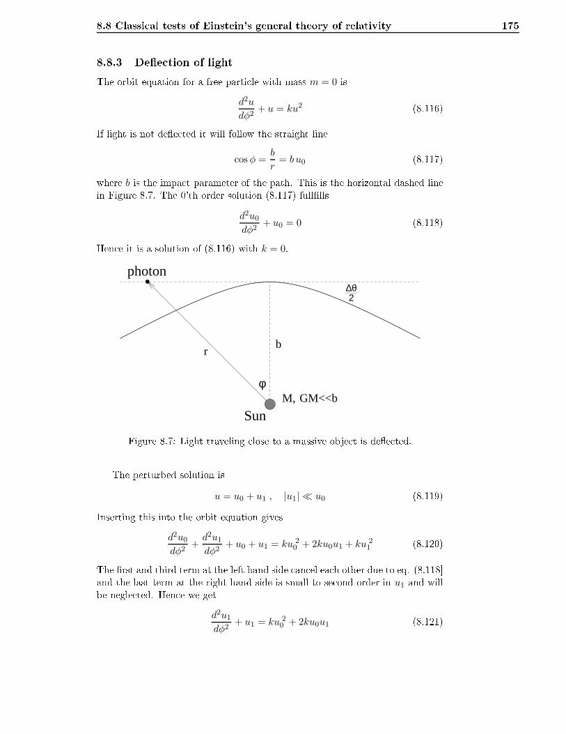
8.8 Classi al tests of Einstein's general theory of relativity 1758.8.3 Dee tion of lightThe orbit equation for a free parti le with mass m = 0 isd2u

dφ2+ u = ku2 (8.116)If light is not dee ted it will follow the straight line

cosφ =b

r= b u0 (8.117)where b is the impa t parameter of the path. This is the horizontal dashed linein Figure 8.7. The 0'th order solution (8.117) fulllls

d2u0

dφ2+ u0 = 0 (8.118)Hen e it is a solution of (8.116) with k = 0.

photon

φ

2

SunM, GM<<b

br

∆θ

Figure 8.7: Light traveling lose to a massive obje t is dee ted.The perturbed solution isu = u0 + u1 , |u1| ≪ u0 (8.119)Inserting this into the orbit equation gives

d2u0

dφ2+d2u1

dφ2+ u0 + u1 = ku 2

0 + 2ku0u1 + ku 21 (8.120)The rst and third term at the left hand side an el ea h other due to eq. (8.118and the last term at the right hand side is small to se ond order in u1 and willbe negle ted. Hen e we get

d2u1

dφ2+ u1 = ku 2

0 + 2ku0u1 (8.121)

176 Chapter 8. The S hwarzs hild spa etimeThe last term at the right hand side is mu h smaller then the rst, and will alsobe negle ted. Inserting for u0 from (8.117) we then getd2u1

dφ2+ u1 =

k

b2cos2 φ (8.122)This equation has a parti ular solution of the form

u1p = A+B cos2 φ (8.123)Inserting this into (8.122) we ndA =

2k

3b2, B = − k

3b2(8.124)Hen e

u1p =k

3b2(2 − cos2 φ

) (8.125)giving1

r= u = u0 + u1 =

cosφ

b+

k

3b2(2 − cos2 φ

) (8.126)The dee tion of the light ∆θ is assumed to be small. We therefore put φ =π2 + ∆θ

2 where ∆θ ≪ π, (see Figure 8.7). Hen ecosφ = cos

(π

2+

∆θ

2

)= − sin

∆θ

2≈ ∆θ

2(8.127)Thus, the term cos2 φ in (8.126) an be negle ted. Furthermore, the dee tionof the light is found by letting r → ∞, i. e. u→ 0. Then we get

∆θ =4k

3b(8.128)For motion in the S hwarzs hild spa etime outside the Sun, k = 3

2RS where RSis the S hwarzs hild radius of the Sun. And for light passing the surfa e of theSun b = R⊙ where R⊙ is the a tual radius of the Sun. The dee tion is then∆θ = 2

RSR⊙

= 1.75′′ (8.129)

Problems 177Problems8.1. The urvature tensor of a sphereIntrodu e an orthonormal basis on the sphere, S2, and use Cartan's stru turalequations to nd the physi al omponents of the Riemann urvature tensor.8.2. The urvature s alar of a surfa e of simultaneityThe spatial line-element of a rotating dis isdℓ2 = dr2 +

r2

1 − ω2r2

c2

dφ2. (8.130)Introdu e an orthonormal basis on this surfa e and use Cartan's stru tural equa-tions to nd the Ri i s alar.8.3. Non-relativisti Kepler motion(a) In the rst part of this ex er ise we will onsider the gravitational potentialin a distan e of r from the Sun to be given by V (r) = −GMr , where Mis the mass of the Sun.Write down the lassi al Lagrangian in spheri al oordiantes (r, θ, φ) for a planet with mass m moving in this eld. TheSun is assumed to be stationary.What is the physi al interpretation of the anoni al momenta pφ = ℓ?How is it possible, by just looking at the Lagrangian, to state that pφ is a onstant of motion? Find The Euler equation for θ and show that it anbe written into the following form

d

dt

(mr4θ2 +

ℓ2

m sin2 θ

)= 0. (8.131)Based on the above equation, show that the planet moves in a plane by hoosing a dire tion of the z-axis so that at a given time, t = 0, we havethat θ = π

2 and θ = 0.(b) Write down the Euler equation for r and use this equation to nd u = 1r asa fun tion of φ. Show that the orbits that des ribe bound staes are ellipti .Find the period T0 for a ir ular orbit given by the radius R in the ir le.( ) If the Sun is not entirely spheri al, but rather a bit deformed (i.e. moreat near the poles), the gravitational eld in the plane where the Sun hasits greatest extension will be modied into

V (r) = −GMr

− Q

r3. (8.132)

Q is a small onstant. We now assume that the motion of the planet takespla e in the plane where the expression of V (r) is valid. Show that a ir ular motion is still possible. What is the period T now, expressed bythe radius R?

178 Chapter 8. The S hwarzs hild spa etime(d) We now assume that the motion deviates slightly from a pure ir ular orbit,that is u = 1R+u1, where u1 ≪ 1

R . Show that u1 varies periodi ally aroundthe orbit,u1 = k sin(fφ). (8.133)Find f and show that the path rotates in spa e for ea h orbit. What is thesize of the angle ∆φ that the planetary motion rotates for ea h orbit?The onstant Q an be written as Q = 1

2J2GMR2s where J2 is a parameterdes ribing the quadrupol mooment and Rs is the radius f the Sun. Obser-vational data indi ate that J2 . 3 · 10−5. Cal ulate how large the rotation

∆φ of the orbit of Mer ury this maximally an ause. Is this su ient toexplain the observed perihelmotion of Mer ury?8.4. The linear eld approximationWe now assume that the gravitational eld i weak, and introdu e a near- atesian oordinate system. The metri then des ribes small deviations from Minkowskispa etime and the metri tensor is given by gµν = ηµν + hµν where ηµν is theMinkowski metri , hµν ≪ 1 and hµν,λ is small.Einstein's eld equations are Rµν− 12gµνR = 8πGTµν , where the units are hosenso that c = 1. Rµν is the Ri i tensor and R ≡ Rββ er den s alar urvaturetensor. Rµν = Rαµαν where

Rαµβν = Γαµν,β − Γαµβ,ν + ΓαλβΓλµν − ΓαλνΓ

λµβ (8.134)is the Riemann urvature tensor..In teh linear approximation we wil only al ulate to 1. order in the metri perturbation h. Show that the the Ri i tensor now an be written as

Rµν =1

2

(h αµα,ν + h α

να,µ − h αµν,α − h,µν

) (8.135)where h ≡ h αα = ηαβhαβ .Show that Einsteins eld equations in this linear approximation an be writtenas

h αµα,ν + h α

να,µ − h αµν,α − h,µν − ηµν(h

αβαβ, − h β

,β ) = 16πGTµν (8.136)This equation an be simplied by introdu ing hµν = hµν− 12ηµνh. Assume that

h satises the ondition h αµα, = 0 (Lorenz gauge). Show that the eld equations an be written as

h αµν,α = −16πGTµν (8.137)8.5. The gravitational potential outside a stati mass distributionA point mass with the mass m is situated in the origin of the nearly- artesian oordinate system seen in 8.4. Its energy-momenta tensor is T00 = mδ(~r),

Tµj = 0 (µ = 0, i), where δ(~r) is the three-dimensional δ-fun tion.

Problems 179(a) Show that, when writing the eld equations in the linear eld approxima-tion on the formhµν,α

α = −16πGTµν , (8.138)then the solution in this ase ish00 =

4Gm

r, der r = (x2 + y2 + z2)1/2 (8.139)

hµi = 0. (8.140)(b) Show that hµν = hµν − 12ηµν h and nd the expression of the innitesimalline element outside the point mass.( ) Introdu e spheri al oordinates and ompare with the line elements in 8.6a) when these metri s are written to the 1. order in M/r (or alternatively

M/ρ). What do you observe??8.6. The S hwarzs hild solution expressed in isotropi oordinates(a) We introdu e a new and radial oordinate ρ so that the S hwarzs hildmetri gets the following form (with units G = c = 1)ds2 = −

(1 − 2M

r

)dt2 +

(1 − 2M

r

)−1

dr2 + r2dΩ2 (8.141)= −

(1 − 2M

r(ρ)

)dt2 + f2(ρ)(dρ2 + ρ2dΩ2) (8.142)where dΩ2 = dθ2 + sin2 θdφ2. Find the fun tions r(ρ) and f(ρ), andwrite down the expli it expression of the line element with ρ as the radial oordinate.(b) What is the value of ρ at the S hwarzs hild horizon? r = 2M? and at theorigin, r = 0? The S hwarzs hild - oordinates t and r inter hange theirroles as r < 2M What is the behaviour of ρ inside the horizon?8.7. The perihelion pre ession of Mer ury and the osmologi al onstant(a) When the osmologi al onstant Λ is non-zero, the Einstein equation takethe form Eµν = −Λgµν . Generalize the S hwarzs hild solution in this aseby showing that the metri is

ds2 = −(1 − 2M

r− 1

3Λr2)dt2 +

dr2

1 − 2Mr − 1

3Λr2+ r2dΩ2, (8.143)where units are hosen so that c = G = 1.(b) Show that the orbit equation for free parti les in the metri given in a) hasthe form (when u = 1

r )d2u

dφ2+ u =

M

L2+ 3Mu2 − Λ

3L2u3. (8.144)

L is the angular momentum pr. mass unit for the parti le.

180 Chapter 8. The S hwarzs hild spa etime( ) Find the perihelion pre ession per rotation given by the new orbit equation.(Hint: Assume that the orbit an be des ribed as a perturbation of a ir le.)(d) Estimations without the Λ-term lead to a orrelation with observations toa pre ision of 1 ar se ond pr. entury. Whi h limitations on the value ofΛ does this lead to?8.8. Gravitational wavesWe will here onsider gravitational waves in the weak eld approximation ofEinstein's equations using the Maxwell equations for the gravitoele tromagneti elds.(a) Use these equations for va uum, and the Lorenz gauge ondition,

1

c

∂φ

∂t+

1

2∇ · Ato show that φ and A satisfy the wave equations

φ = 0,

A = 0, (8.145)where is the d'Alembert operator in Minkowski spa e. Hen e, not sur-prisingly, gravitational waves travel with the speed of light. We an assumethat A has in general omplex omponents. The physi al ve tor potentialis the real part of A.(b) Consider waves far from any sour es, so that φ = 0. Find parti ular so-lutions where the wave des ribes a plane-wave with wave-ve tor k. Whatdoes the Lorenz gauge ondition tell us about the nature of these gravita-tional waves?( ) A test parti le is initially at rest as one of the plane waves with wave-ve tork = kex passes by. The wave is plane-polarised so that A an be written

A = A0eik(x−ct), (8.146)where A0 = A0ey, and A0 real. Assume that the test parti le is pla edat the origin and that the deviation from the origin as the wave passesby is very small ompared to the wavelength of the wave. Hen e, we anassume that eik(x−ct) ≈ e−ikct. Assume also that the speed of the parti le

v is non-relativisti : v/c ≪ 1 (thus A0 has to be su iently small). Usethe Lorentz for e law for GEM elds and derive the the position of theparti le to lowest order in A0/c2 as the wave passes by.(d) Explain why gravitational waves annot have only a Newtonian part, andthus that there are no gravitational waves in the Newtonian theory (or thatthey move with innite speed).8.9. Plane-wave spa etimesWe will in this problem onsider the plane wave metri

ds2 = 2du(dv +Hdu) + dx2 + dy2, (8.147)

Problems 181where the fun tion H = H(u, x, y) does not depend on v (but is otherwisearbitrary).(a) From the above we have the metri omponents given by guv = 1, guu = 2Hand gxx = gyy = 0. What is gµν? Cal ulate also the Christoel symbolsand show that the ve tor k = ∂dv is onvariantly onstant; i.e., kµ;ν = 0.Is k time-like, null or spa e-like?(b) Use the Christoel symbols to al ulate the Einstein tensor and show thatin va uum (Λ = 0) the Einstein eld equations redu e to(∂d2x2 + ∂d2y2

)H = 0. (8.148)What are the linearised eld equations in this ase?( ) Show that

H = C1(u)(x2 − y2) + 2C2(u)xy,where C1(u) and C2(u) are arbitrary fun tions of u, is a solution to Ein-stein's eld equations.Consider the omplex oordinate z = x + iy, and an arbitrary analyti omplex fun tion f(u, z). Show that

H = f(u, z) + f(u, z),where a bar means omplex onjugate, is a solution to Einstein's eldequations. Is it also a solution to the linear eld equations?8.10. Embedding of the interior S hwarzs hild metri Make an embedding of the three-dimensional spatial se tion t = 0 of the in-ternal S hwarzs hild solution. Join the resulting surfa e to the orrespondingembedding of the external S hwarzs hild solution.8.11. The S hwarzs hild-de Sitter metri In this problem we will solve the Einstein equations with a osmologi al on-stant. The Einstein equations with a osmologi al onstant Λ an be writtenRµν −

1

2Rgµν + Λgµν = κGTµν (8.149)(a) Use S hwarzs hild oordinates and solve the Einstein va uum equationswith a osmologi al onstant.(b) Show that in this ase there are two horizons. Set the mass parameterequal to zero, and show that the spatial se tions dt = 0 an be onsideredas a 3-sphere, S3.8.12. Proper radial distan e in the external S hwarzs hild spa eShow that the proper radial distan e from a oordinate position r to the horizon

RS in the external S hwarzs hild spa e isℓr =

√r√r −RS +RS ln

(√r

RS−√

r

RS− 1

).Find the limit of this expression for RS ≪ r.

182 Chapter 8. The S hwarzs hild spa etime8.13. Gravitational redshift in the S hwarzs hild spa etimeDene z, des ribing the redshift of light, byz =

∆λ

λe, (8.150)where ∆λ is the hange in the photons wavelength and λe the wavelength of thephoton when emitted.Show that the gravitational redshift of light emitted at rE and re eived at rRin the S hwarzs hild spa etime outside a star of mass M is

z =

(rR −RSrE −RS

) 12

− 1where RS = 2M is the S hwarzs hild radius of the star. What is the gravita-tional redshift of light emitted from the surfa e of a neutron star as observedby a faraway observer? A neutron star has typi ally a mass of 1.2 solar massesand a radius of about 20km.

Chapter 9Bla k Holes9.1 'Surfa e gravity': gravitational a eleration onthe horizon of a bla k holeSurfa e gravity is denoted by κ1 and is dened byκ = lim

r→r+

a

uta =

√aµaµ (9.1)where r+ is the horizon radius, r+ = RS for the S hwarzs hild spa etime, ut isthe time omponent of the 4-velo ity.The 4-velo ity of a free parti le instantanously at rest in the S hwarzs hildspa etime:

~u = ut~et =dt

dτ~et =

1√−gtt~et =

~et√1 − RS

r

(9.2)The only omponent of the 4-a eleration dierent from zero, is ar. The4-a eleration:~a = ∇~u~u = uµ;νuν~eµ = (uµ,ν + Γµανuα)uν~eµ.ar = (ur,ν + Γrανu

α)uν

= ur,νuν

︸ ︷︷ ︸=0

+Γrtt(ut)2

=Γrtt

1 − RS

r

Γrtt = −1

2

∂gtt∂r

= −RS2r2

ar =RS

2r2

1 − RS

r

ar = grrar =argrr

= (1 − RSr

)ar =RS2r2

(9.3)The a eleration s alar: a =

√arar =

RS2r2q1−RS

r

(measured with standard instru-183

184 Chapter 9. Bla k Holesments: at the horizon, time is not running).a

ut=RS2r2

(9.4)With :a

ut=c2RS2r2

=GM

r2(9.5)

κ = limr→RS

a

ut=

1

2RS=

1

4GM(9.6)In luding c the expression is κ = c2

4GM . On the horizon of a bla k hole with onesolar mass, we get κ⊙ = 2 × 1013 ms2 .9.2 Hawking radiation:radiation from a bla k holeThe radiation from a bla k hole has a thermal spe trum. We are going to 'nd'the temperature of a S hwarzs hild bla k hole of mass M. The Plan k spe trumhas an intensity maximum at a wavelength given by Wien's displa ement law.

Λ =N~c

kTwhere k is the Boltzmann onstant, and N=0.2014For radiation emitted from a bla k hole, Hawking derived the following expres-sion for the wavelength at a maximum intensity

Λ = 4πNRS =8πNGM

c2(9.7)Inserting Λ from Wien's displa ement law, gives:

T =~c3

8πGkM=

~c

2πkκ (9.8)Inserting values for ~, c and k gives:

T ≈ 2 × 10−4m

RSK (9.9)For a bla k hole with one solar mass,we have T⊙ ≈ 10−7. When the mass isde reasing be ause of the radiation, the temperature is in reasing.So a bla khole has a negative heat apa ity. The energy loss of a bla k hole be ause ofradiation, is given by the Stefan-Boltzmann law:

−dMdt

= σT 4A

c2(9.10)where A is the surfa e of the horizon.

A = 4πR2S =

16πG2M2

c4(9.11)

9.3 Rotating Bla k Holes: The Kerr metri 185gives:−dMdt

=1

15360π

~c6

G2M2≡ Q

M2

M(t) = (M30 − 3Qt)1/3, M0 = M(0)

(9.12)A bla k hole with mass M0 early in the history of the universe whi h is aboutto explode now, had to have a starting massM0 = (3Qt0)

1/3 ≈ 1012kg (9.13)about the mass of a mountain. They are alled 'mini bla k holes'.9.3 Rotating Bla k Holes: The Kerr metri This solution was found by Roy Kerr in 1963.A time-independent, time-orthogonal metri is known as a stati metri . Atime-independent metri is known as a stationary metri . A stationary metri allows rotation.Consider a stationary metri whi h des ribes a axial-symmetri spa eds2 = −e2νdt2 + e2µdr2 + e2ψ(dφ− ωdt)2 + e2λdθ2 , (9.14)where ν, µ, ψ, λ and ω are fun tions of r and θ.By solving the va uum eld equations for this line-element, Kerr found thesolution:

e2ν =ρ2∆

Σ2, e2µ =

ρ2

∆, e2ψ =

Σ2

ρ2sin2 θ , e2λ = ρ2 ,

ω =2Mar

Σ2, where ρ2 = r2 + a2 cos2 θ

∆ = r2 + a2 − 2Mr

Σ2 = (r2 + a2)2 − a2∆ sin2 θ(9.15)This is the Kerr solution expressed in Boyer-Lindquist oordinates. The fun tionω is the angular-velo ity. The Kerr-solution is the metri for spa e-time outsidea rotating mass-distribution. The onstant a is spin per mass-unit for the mass-distribution and M is its mass.Line-element:

ds2 = −(1 − 2Mr

ρ2)dt2 +

ρ2

∆dr2 − 4Mar

ρ2sin2 θdtdφ+ ρ2dθ2

+ (r2 + a2 +2Ma2r

ρ2sin2 θ) sin2 θdφ2

(9.16)(Here M is a measure of the mass so that M = G · mass, ie. G = 1)

186 Chapter 9. Bla k HolesLight emitted from the surfa e, r = r0, where g tt = 0 is innitely redshiftedfurther out. Observed from the outside time stands still.ρ2 = 2Mr0 ⇒ r20 + a2 cos2 θ = 2Mr0

r0 = M ±√M2 − a2 cos2 θ

(9.17)This is the equation for the surfa e whi h represents innite redshift.9.3.1 Zero-angular-momentum-observersThe Lagrange fun tion of a free parti le in the equator plane, θ = π2

L = −1

2(e2ν − ω2e2ψ)t2 +

1

2e2µr2 +

1

2e2ψφ2 +

1

2e2λθ2 − ωe2ψ tφ (9.18)Here θ = 0. The momentum pφ of the y li oordinates φ:

pφ ≡ ∂L

∂φ= e2ψ(φ− ωt) , t =

dt

dτ, φ =

dφ

dτ(9.19)The angular speed of the parti le relative to the oordinate system:

Ω =dφ

dt=φ

t, φ = Ωt

⇒ pφ = e2ψ t(Ω − ω)

(9.20)pφ is onserved during the movement.

ω = − gtφgφφ

=2Mar

(r2 + a2)2 − a2(r2 + a2 − 2Mr),

ω → 0 when r → ∞(9.21)When studying the Kerr metri one nds that Kerr → Minkowski for large

r. The oordinate lo ks in the Kerr spa e-time show the same time as thestandard- lo ks at rest in the asymptoti Minkowski spa e-time.A ZAMO is per denition a parti le or observer with pφ = 0. Consider afar away observer who let a stone fall with vanishing initial velo ity. pφ is a onstant of motion, so the stone remains a ZAMO during the movement. Alo al referen e frame whi h oin ides with the stone is a member of the lassof inertial frames that are at rest in the asymptoti Minkowski region. TheseZAMO nertial frames may be used to dene the state of motion of the spa e.They have .pφ = 0 ⇒ Ω =

dφ

dt= ω (9.22)That is, the lo al inertial frame obtains an angular speed relative to the BL-system (Boyer-Lindquist system).Sin e the Kerr metri is time independent, the BL-system is sti. Thedistant observer has no motion relative to the BL-system. To this observer the

9.3 Rotating Bla k Holes: The Kerr metri 187BL-system will appear sti and non-rotating. The observer will observe thatthe lo al inertial system of the stone obtains an angular speeda is spinper massunity andMa is spin dφ

dt= ω =

2Mar

(r2 + a2)2 − a2(r2 + a2 − 2Mr)(9.23)In other words, inertial systems at nite distan es from the rotating mass Mare dragged with it in the same dire tion. This is known as inertial draggingor the Lense-Thirring ee t (about 1920).9.3.2 Does the Kerr spa e have a horizon?Denition 9.3.1 (Horizon)a surfa e one an enter, but not exit.Consider a parti le in an orbit with onstant r and θ. It's 4-velo ity is:

~u =d~x

dτ=dt

dτ

d~x

dt

= (−g tt − 2g tφΩ − g φφΩ2)−

12 (1,Ω) , where Ω =

dφ

dt

(9.24)To have stationary orbits the following must be trueg φφΩ

2 + 2g tφΩ + g tt < 0 (9.25)This implies that Ω must be in the intervalΩmin < Ω < Ωmax , (9.26)where Ωmin = ω −

√ω2 − g tt

gφφ, Ωmax = ω +

√ω2 − g tt

gφφ

sin e g tφ = −ωg φφ.Outside the surfa e with innite redshift g tt < 0. That is Ω an be negative,zero and positive. Inside the surfa e r = r0 with innite redshift g tt > 0. HereΩmin > 0 and stati parti les, Ω = 0, annot exist. This is due to the inertialdragging ee t. The surfa e r = r0 is therefore known as the stati border.The interval of Ω, where stationary orbits are allowed, is redu ed to zerowhen Ωmin = Ωmax, that is ω2 =

g tt

gφφ

⇒ g tt = ω2g φφ (equation for the horizon).For the Kerr metri we have:g tt = ω2g φφ − e2ν (9.27)Therefore the horizon equation be omes

e2ν = 0 ⇒ ∆ = 0 ∴ r2 − 2Mr + a2 = 0 (9.28)The largest solution is r+ = M +√M2 − a2 and this is the equation for aspheri al surfa e. The stati border is r0 = M +

√M2 − a2 cos θ.

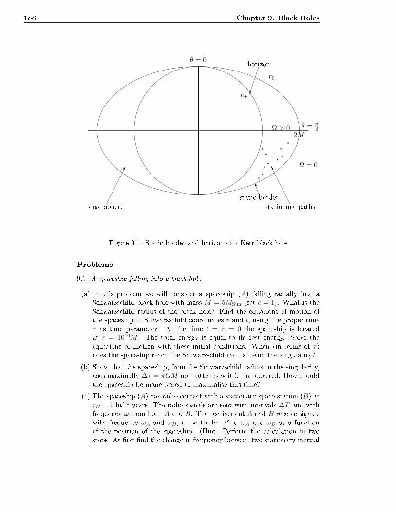
188 Chapter 9. Bla k Holes

ergo-sphere Kstationary pathsMstati border

horizonr+

r0

θ = 0

θ = π2Ω > 0

Ω = 0

2M

Figure 9.1: Stati border and horizon of a Kerr bla k holeProblems9.1. A spa eship falling into a bla k hole(a) In this problem we will onsider a spa eship (A) falling radially into aS hwarzs hild bla k hole with mass M = 5MSun (set c = 1). What is theS hwarzs hild radius of the bla k hole? Find the equations of motion ofthe spa eship in S hwarzs hild oordinates r and t, using the proper timeτ as time parameter. At the time t = τ = 0 the spa eship is lo atedat r = 1010M . The total energy is equal to its rest energy. Solve theequations of motion with these initial onditions. When (in terms of τ)does the spa eship rea h the S hwarzs hild radius? And the singularity?(b) Show that the spa eship, from the S hwarzs hild radius to the singularity,uses maximally ∆τ = πGM no matter how it is maneuvered. How shouldthe spa eship be maneuvered to maximalise this time?( ) The spa eship (A) has radio onta t with a stationary spa e-station (B) atrB = 1 light years. The radio-signals are sent with intervals ∆T and withfrequen y ω from both A and B. The re eivers at A and B re eive signalswith frequen y ωA and ωB, respe tively. Find ωA and ωB as a fun tionof the position of the spa eship. (Hint: Perform the al ulation in twosteps. At rst nd the hange in frequen y between two stationary inertial

Problems 189systems in the points rA (the pos. of the spa eship) and rB. Then al ulatethe hange in frequen y due to a transfer into an inertial system with thevelo ity of teh spa eship.) Investigate whether something parti ular ishappening as the spa eship passes the S hwarzs hild radius. Dis uss whatthese results tell us about how the events in the spa eship is des ribed inthe spa e station, and vi e versa.9.2. The spa etime inside and outside a rotating spheri al shellA spheri al shell with massM and radius R is rotating with a onstant angularvelo ity ω. In this problem the metri inside and outside the shell shall be foundusing the linearised Einstein's eld equationshαβ = −2κTµν , (9.29)where hαβ is the metri perturbation with respe t to the Minkowski metri Therotation is assumed to be non-relativisti , thus the al ulations should be madeto rst order in Rω.Assume that the shell is omposed of dust, so that the energy-momentum tensor an be expressed as

Tαβ = ρuαuβ, ρ =M

4πR2δ(r −R)

uα ≈ (−1,−Rω sin θ sinφ,Rω sin θ cosφ, 0) (9.30)where (r, θ, φ) are spheri al oordinates:x = r sin θ cosφ, y = r sin θ sinφ, r = cos θ. (9.31)Find the metri inside and outside the rotating shell and show that

ds2 = −(

1 − 2M

R

)dt2 +

(1 +

2M

R

)(dx2 + dy2 + dz2)

−8Mω

3Rr2 sin2 θdφdt, r < R

ds2 = −(

1 − 2M

r

)dt2 +

(1 +

2M

r

)(dx2 + dy2 + dz2)

−4J

rsin2 θdφdt, r > R (9.32)where J = (2/3)MR2ω is the angular momentum of the shell. (Hint: Estimate

g0φ rst nding h0y. Due to the axial symmtry we have that g0φ = g1/2φφ [g0y]φ=0.Assume that h0y has the form h0y = f(r) sin θ cosφ.)9.3. Physi al interpretation of the Kerr metri In this problem we shall use the linearised solution of the spa etime outside arotating shell derived in problem 9.2.

190 Chapter 9. Bla k Holes(a) Show that the Kerr metri is redu ed to the metri (9.32) in the limitr > R and r ≫ M and identify thereby the onstant a with the angularmomentum per unit mass of the rotating shell. (Hint: Expand the Kerrmetri to rst order in J/Mr, introdu e isotropi oordinates (r → ρ seeproblem 8.6), and expand the result to rst order in M/ρ).(b) Find the angular velo ity

ωL = − g0φgφφ

(9.33)that lo al referen e frames are rotating with, with respe t to referen eframes at innity.9.4. Kinemati s in 3-spa eA Kerr bla k hole is a ele tri ally neutral, rotating bla k hole. When spa etimeoutside a Kerr bla k hole is des ribed in Boyer-Lindquist (BL) oordinates, theline element is the followingds2 = −e2νdt2 + e2µdr2 + e2λdθ2 + e2ψ(dφ− ωdt)2, (9.34)where

e2ν =ρ2∆

Σ2, e2µ =

ρ2

∆, e2λ = ρ2

e2ψ =

(Σ2

ρ2

)sin2 θ, ω = − gtφ

gφφ=

2Mar

Σ2

ρ2 = r2 + a2 cos2 θ, ∆ = r2 + a2 − 2Mr, Σ2 = (r2 + a2)2 − a2∆ sin2 θHere M is the mass of the hole and a its spin pr. unit mass.(a) Consider light moving in negative and positive dire tion of φ. What is the oordinate velo itycφ =

dφ

dt(9.35)of light?We now want to investigat the Sagna -ee t in the Kerr-spa e. An emitter-re eiver is atta hed to a point in the BL- oordinate systemet. Light signalswith the frequen y ν are sent by means of mirrors in both dire tions alongthe ir le r = r0, θ = π/2. Find the phase dieren e of light travelling inopposite dire tions, when the signals res h the re eiver.The result shows that the BL-system looks like a rotating oordinate sys-tem when observed from a nite distan e r from the bla k hole. Does thebls k hole appear to be rotating when observed from innity? ute?(b) Consider a free parti le in teh Kerr-spa e. Assume that it is moving in thedire tion of φ, with an angular velo ity

Ω = dφ/dt (9.36)

Problems 191given in the BL- oordinates. Write down the Lagrangian L of the parti leand nd its anoni al momentum,pφ = ∂L/∂φ. (9.37)What is the angular velo ity of a parti le with vanishing momentum?( ) A ZAMO (Zero Angular Momentum Observer) is an observer with van-ishing.angular momentum. Consider in parti ular a ZAMO with xed r-and θ- oordinates. Is this ZAMO freely falling?In the following ZAMO will be des ribing the parti ular observers withxed r- and θ- oordinates. Introdu e an orthonormal basis (~et′ , ~er′ , ~eθ′ , ~eφ′),where ~et′ is the 4-velo ity of a ZAMO. The dual basis 1-forms are

ωt′

= eνωt, ωr′

= eµωr,

ωθ′

= eλωθ, ωφ′

= eψ(ωφ − ωωt). (9.38)Show that~et′ = e−ν(~et + ω~eφ), ~er′ = e−µ~er,

~eθ′ = e−λ~eθ, ~eφ′ = e−ψ~eφ, (9.39)where (~et, ~er, ~eθ, ~eφ) are the oordinate basis vek ors in the BL- oordinatesystem.Show that the physi al velo ity of the parti le from part b), measured bya ZAMO, isvφ

′

= eψ−ν(Ω − ω). (9.40)What is the velo ity vφ′0 of a xed oordinate point measured by a ZAMO?(d) Introdu e an orthonormal basis eld given by the expressions~e0 = (−g00)−1/2~e0, ~ei = (γii)

−1/2[~ei − (gi0/g00)~e0] (9.41)whereγii = gii − g2

i0/g00Show that~et = γe−ν~et, ~er = e−µ~er,

~eθ = e−λ~er, ~eφ = γ−1e−ψ~eφ + γe−νvφ′

0 ~et, (9.42)where γ = (1− (vφ′

0 )2)−1/2. Find the duale basis 1-forms. The ve tor ~et isthe 4-velo ity of a parti le at rest in the BL- oordinate systemet, that is,of a stati parti le.(e) Find the physi al velo ity vφ of the parti le from point b), measured bya stati observer. What is the orresponden e between vφ′ , vφ, and vφ

′

0 ?Show that the orthonormal basis eld assosiated with a stati observer andthat assosiated with a ZAMO are related through a Lorentz transforma-tion.

192 Chapter 9. Bla k Holes9.5. The life time of a bla k holeConsider a bla k hole in a zero-temperature heat-bath. In luding c, ~, kB andG we have M = Gmc−2, the bla k hole temperature is

T =~

2πkBcκ (9.43)and the Stefan-Boltsmann onstant is

σ =π2k4

B

60~3c2(9.44)(a) Assume that a bla k hole has a mass m0 at t = 0. Find m(t).(b) If we onsider a time span of approximately τ = 1010 years, what masswould the bla k hole have at t = 0 to have m(τ) = 0?( ) Show that a bla k hole of mass m annot disintegrate into two smallerbla k holes of mass m1 and m2 where m = m1 +m2.9.6. A gravitomagneti lo k ee tThis problem is on erned with the dieren e of proper time shown by two lo ksmoving freely in opposite dire tions in the equatorial plane of the Kerr spa etimeoutside a rotating body. The lo ks move along a path with r = constant and

θ = π/2.(a) Show that in this ase the radial geodesi equation redu es toΓrttdt

2 + 2Γrφtdφdt + Γrφφdφ2 = 0.(b) Cal ulate the Christoel symbols and show that the equation takes theform (

dt

dφ

)2

− 2adt

dφ+ a2 − r3

M= 0,where M is the mass of the rotating body and a its angular momentumper unit mass, a = J/M .( ) Use the solution of the geodesi equation and the four-velo ity identity toshow that the proper time interval dτ shown on a lo k moving an angle

dφ isdτ = ±

√1 − 3M

r± 2aω0dφ,where ω0 =

(M/r3

)1/2 is the angular velo ity of a lo k moving in theS hwarzs hild spa etime in a ordan e with Kepler's 3rd law. The plusand minus sign apply to dire t and retrograde motion, respe tively.(d) Show that to rst order in a the proper time dieren e for one losed orbit(φ→ φ+2π) in the dire t and the retrograde dire tion is τ+− τ− ≈ 4πa =4πJ/M , or in S.I. units, τ+ − τ− ≈ 4πa = 4πJ/mc2.Estimate this time dieren e for lo ks in satellites moving in the equatorialplane of the Earth. (The mass of the Earth ism = 6·1026kg and its angularmomentum J = 1034kg m2s−1.)

Problems 1939.7. The photon sphere radius of a Reissner-Nordström bla k holeShow that there exists a sphere of radiusrPS =

3M

2

(1 +

√1 − 8Q2

9M2

) (9.45)in the Reissner-Nordström bla k hole spa etime where photons will have ir ularorbits around the bla k hole.9.8. The Reissner-Nordström repulsionConsider a radially infalling neutral parti le in the Reissner-Nordström spa e-time with M > |Q|. Show that when the parti le omes inside the radiusr = Q2/M it will feel a repulsion away from r = 0 (i.e. that d2r/dτ2 < 0 for τthe proper time of the parti le). Is this inside or outside the outer horizon r+?Show further that the parti le an never rea h the singularity at r = 0.9.9. Gravitational mass(a) Use the general S hwarzs hild line-element and show that the surfa e grav-ity of a S hwarzs hild bla k hole an be written

κ = −eα−βα′. (9.46)(b) Show, using Einstein's eld equations, that4πr2eα+β

(T 0

0 − T 11 − T 2

2 − T 33

)=(r2eα−βα′

)′. (9.47)Hen e, dedu e that the surfa e gravity an be written

κ = −4π

r2

∫ r

0

(T 0

0 − T 11 − T 2

2 − T 33

)eα+βr2dr. (9.48)( ) Dene the gravitational mass MG inside a radius r of a spheri al massdistribution by

κ = −MG

r2, (9.49)and dedu e that

MG = 4π

∫ r

0

(T 0

0 − T 11 − T 2

2 − T 33

)eα+βr2dr. (9.50)This is the Tolman-Whittaker expression for the gravitational mass of asystem.What is the ondition for repulsive gravitation?9.10. The river model for bla k holesIn this problem you are going to pi ture spa e as owing like a river into aS hwarzs hild bla k hole Spa e is then represented by a ontinuum of lo alinertial frames falling freely from zero velo ity at innity.

194 Chapter 9. Bla k Holes(a) Show that the S hwarzs hild metri may be written in the Gullstrand-Painlevé formds2 = −dτ2 + (dr + βdτ)2 + r2(dθ2 + sin2 dφ2), β =

√rSr,by introdu ing a new oordinate time

τ = t+ 2rS

(1

β− arctanhβ

).(b) Show that β(r) = −dr/dτ is the velo ity of an inertial frame falling freelyfrom rest at innity, i.e., the river velo ity. What happens at the horizonof the bla k hole? Show that dτ is the proper time interval as measuredby a lo k omoving with the inertial frames that dene the river model ofthe spa e.

Chapter 10S hwarzs hild's Interior Solution10.1 Newtonian in ompressible star∇2φ = 4πGρ, φ = φ(r)

1

r2d

dr(r2

dφ

dr) = 4πGρ

(10.1)Assuming ρ = constant.d(r2

dφ

dr) = 4πGρr2dr

r2dφ

dr=

4π

3Gρr3 +K

= M(r) +K

(10.2)Gravitational a eleration: ~g = −∇φ = −dφdr~er

g =M(r)

r2+K1

r2=

4π

3Gρr +

K1

r2(10.3)Finite g in r = 0 demands K1 = 0.

g =4π

3Gρr,

dφ

dr=

4π

3Gρr (10.4)Assume that the massdistribution has a radius R.

φ =2π

3Gρr2 +K2 (10.5)Demands ontinuous potensial at r = R.

2π

3GρR2 +K2 =

M(R)

R= −4π

3GρR2

⇒ K2 = −2πGρR2(10.6)(with zero level at innite distan e). Gives the potensial inside the mass distri-bution:

φ =2π

3Gρ(r2 − 3R2) (10.7)195

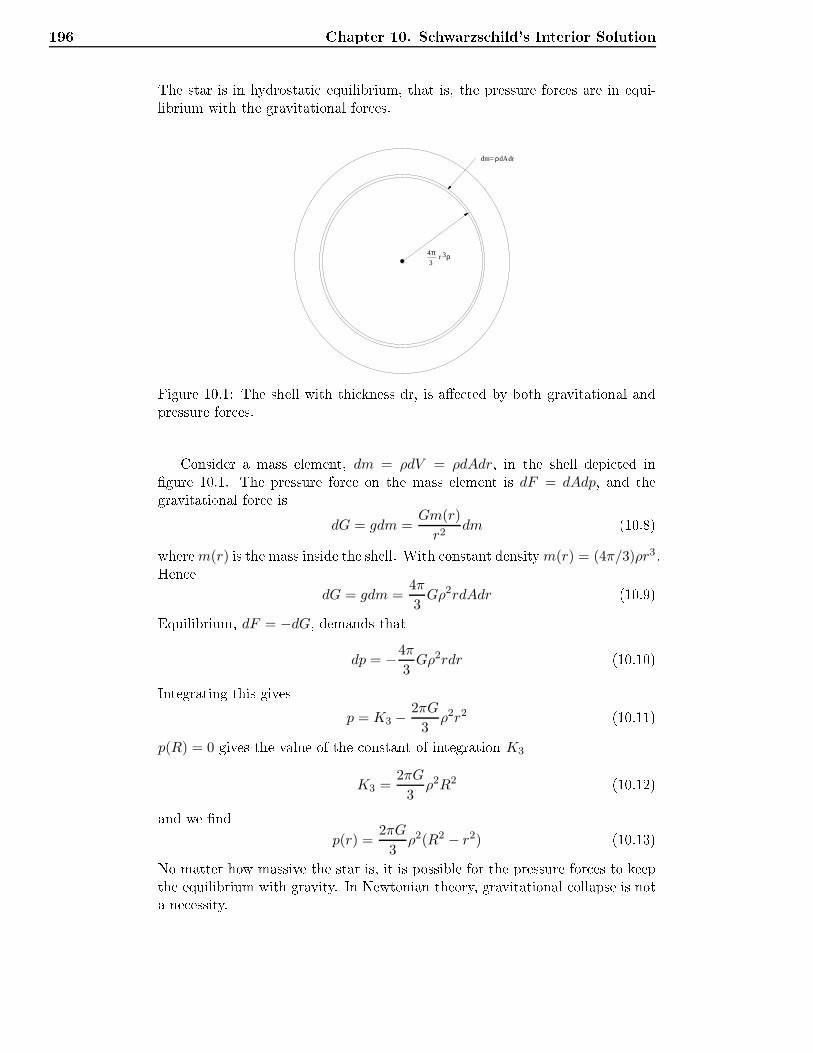
196 Chapter 10. S hwarzs hild's Interior SolutionThe star is in hydrostati equilibrium, that is, the pressure for es are in equi-librium with the gravitational for es.4π3

ρ

r ρ3

dm= drdA

Figure 10.1: The shell with thi kness dr, is ae ted by both gravitational andpressure for es.Consider a mass element, dm = ρdV = ρdAdr, in the shell depi ted ingure 10.1. The pressure for e on the mass element is dF = dAdp, and thegravitational for e isdG = gdm =

Gm(r)

r2dm (10.8)wherem(r) is the mass inside the shell. With onstant densitym(r) = (4π/3)ρr3.Hen e

dG = gdm =4π

3Gρ2rdAdr (10.9)Equilibrium, dF = −dG, demands that

dp = −4π

3Gρ2rdr (10.10)Integrating this gives

p = K3 −2πG

3ρ2r2 (10.11)

p(R) = 0 gives the value of the onstant of integration K3

K3 =2πG

3ρ2R2 (10.12)and we nd

p(r) =2πG

3ρ2(R2 − r2) (10.13)No matter how massive the star is, it is possible for the pressure for es to keepthe equilibrium with gravity. In Newtonian theory, gravitational ollapse is nota ne essity.

10.2 The pressure ontribution to the gravitational mass of a stati , spheri allysymmetri system 19710.2 The pressure ontribution to the gravitationalmass of a stati , spheri ally symmetri systemWe now give a new denition of the gravitational a eleration (not equivalentto (8.23))g = − a

ut, a =

√aµaµ (10.14)We have the line element:

ds2 = −e2α(r)dt2 + e2β(r)dr2 + r2dΩ2

gtt = −e2α , grr = e2β(10.15)gives (be ause of the gravitational a eleration)

g = −eα−βα′ (10.16)From the expressions for Ett, E rr, E θθ

, Eφφ

follow (see Se tion 8.1)E tt− E rr − Eθ

θ− Eφ

φ= −2e−2β(

2α′

r+ α′′ + α′2 − α′β′) . (10.17)We also have

(r2eα−βα′)′= r2eα−β(

2α′

r+ α′′ + α′2 − α′β′) , (10.18)whi h gives

g = +1

2r2

∫(E t

t− E rr − Eθ

θ−Eφ

φ)r2eα+βdr . (10.19)By applying Einstein's eld equations

Eµν = 8πGT µν (10.20)we getg = +

4πG

r2

∫(T tt− T rr − T θ

θ− T φ

φ)r2eα+βdr . (10.21)This is the Tolman-Whittaker expression for gravitational a eleration.The orresponding Newtonian expression is :

gN = −4πG

r2

∫ρr2dr (10.22)The relativisti gravitational mass density is therefore dened as

ρG = −T tt+ T rr + T θ

θ+ T φ

φ(10.23)

198 Chapter 10. S hwarzs hild's Interior SolutionFor an isotropi uid withT tt= −ρ , T rr = T θ

θ= T φ

φ= p (10.24)we get ρG = ρ+ 3p (with c = 1), whi h be omes

ρG = ρ+3p

c2(10.25)It follows that in relativity, pressure has a gravitational ee t. Greater pressuregives in reasing gravitational attra tion. Strain (p < 0) de reases the gravita-tional attra tion.In the Newtonian limit, c→ ∞, pressure has no gravitational ee t.10.3 The Tolman-Oppenheimer-Volkov equationWith spheri al symmetry the spa etime line-element may be written

ds2 = −e2α(r)dt2 + e2β(r)dr2 + r2dΩ2

Ett

= 8πGTtt, T µν = diag(−ρ, p, p, p)

(10.26)From Ettwe get

1

r2d

dr[r(1 − e−2β)] = 8πGρ

r(1 − e−2β) = 2G

∫ r

04πρr2dr ,

(10.27)where m(r) =∫ r0 4πρr2dr giving

e−2β = 1 − 2Gm(r)

r=

1

g rr(10.28)From E rr we have

E rr = 8πGT rr

2

r

dα

dre−2β − 1

r2(1 − e−2β) = 8πGp

(10.29)We get2

r

dα

dr(1 − 2Gm(r)

r) − 2Gm(r)

r3= 8πGp

dα

dr= G

m(r) + 4πr3p(r)

r(r − 2Gm(r))(10.30)

10.3 The Tolman-Oppenheimer-Volkov equation 199The relativisti generalized equation for hydrostati equilibrium is T rν;ν = 0,givingT rν,ν + ΓνανT

rα + ΓrανTαν = 0

T rν,ν = T rr,r = p ,r =1

√g rr

∂p

∂r

T rν,ν = e−βdp

dr

ΓνανTrα = Γνrνp = Γt

rtp+ Γαrαp

ΓrανTαν = ΓrννT

νν = Γrttρ+ Γrααp

(10.31)In orthonormal basis we have

Ω νµ = −Ω µν ⇒ Γ µνα = −Γ νµα

Γαrα = Γ αrα = −Γ rαα = −Γrαα(10.32)

T rν;ν = 0 now takes the form:e−β

dp

dr+ Γt

rtp+ Γr

ttρ = 0 (10.33)We have

Γtrt

= −Γtrt

= Γrtt

= Γrtt

(10.34)and we also have Γrtt

= e−β dαdr , giving:dp

dr+ (p+ ρ)

dα

dr= 0 (10.35)Inserting Equation 10.30 into Equation 10.35 gives

dp

dr= −G(ρ+ p)

m(r) + 4πr3p(r)

r(r − 2Gm(r))(10.36)This is the Tolman-Oppenheimer-Volkov (TOV) equation. The omponent gtt =

−e2α(r) may now be al ulated as followsdp

ρ+ p= −dα , ρ = onstant

ln(ρ+ p) = K − α

ρ+ p = K1e−α , p = K1e

−α − ρ

(10.37)Hen eeα = eα(R)(1 +

p

ρ)−1 (10.38)where R is the radius of the mass distribution.

200 Chapter 10. S hwarzs hild's Interior Solution10.4 An exa t solution for in ompressible stars - S hwarzs hild'sinterior solutionThe mass inside a radius r for an in ompressiable star ism(r) =

4

3πρr3 (10.39)

e−2β = 1 − 2Gm(r)

r≡ 1 − r2

a2(10.40)where

a2 =3

8πGρ, m(r) =

r3

2Ga2, rs = 2Gm =

r2

a2r (10.41)TOV equation:

dp

dr= −G

43πρr

3 + 4πr3p(r)

r(r − 2G43πρr

3)(ρ+ p(r))

= −G4

3πρ+ 3p(r)

1 −G83πρr

2r(ρ+ p(r))

= − 1

2a2ρ

ρ+ 3p(r)

1 − r2

a2

r(ρ+ p(r))

⇒∫ p

0

dp

(ρ+ 3p)(ρ+ p= − 1

2a2ρ

∫ r

R

r

1 − r2

a2

dr

p+ ρ

3p + ρ=

√a2 −R2

a2 − r2

(10.42)So the relativisti pressure distribution is

p(r) =

√a2 − r2 −

√a2 −R2

3√a2 −R2 −

√a2 − r2

ρ, ∀r ≤ R (10.43)alsoa2 =

3

8πGρ,a2

r2=

r

rs> 1 ⇒ a > r (10.44)To satisfy the ondition for hydrostati equilibrium we must have p > 0 or

p(0) > 0 whi h givesp(0) ≡ pc =

a−√a2 −R2

3√a2 −R2 − a

> 0 (10.45)in whi h the numerator is positive so that3√a2 −R2 > a

9a2 − 9R2 > a2

R <

√8

9a

R2 <8

9a =

8

9

3

8πGρ=

1

3πGρ

(10.46)

Problems 201Stellar mass:M =

4

3πρR3 <

4

3πρR

1

3πGρ=

4R

9G

M <4

9G

1√3πGρ

(10.47)For a neutron star we an use ρ ≈ 1017 g /cm3. An upper limit on the mass isthen M < 2.5 M⊙ Substitution for p in the expression for eα giveseα =

3

2

√1 − Rs

R− 1

2

√1 − Rs

R3r2 (10.48)The line element for the interior S hwarzs hild solution is

ds2 = −(

3

2

√1 − Rs

R− 1

2

√1 − Rs

R3r2

)2

dt2 +dr2

1 − Rs

R3 r2+ r2dΩ, r ≤ R(10.49)Problems10.1. Curvature of 3-spa e and 2-surfa es of the internal and the external S hwarzs hildspa etimes(a) The 3-spa e of the internal S hwarzs hild solution has a geometry given bythe line-element

dℓ2I =dr2

1 − RS

R2 r2+ r2(dθ2 + sin2 θdφ2)where RS = 2M is the S hwarzs hild radius of the mass distribution and Rits radius. The orresponding line-element for the external S hwarzs hildsolution is

dℓ2E =dr2

1 − RS

r

+ r2(dθ2 + sin2 θdφ2)Find the spatial urvature k = k(r) = 16R of the 3-spa es, where R is theRi i s alar.(b) We shall now onsider the equatorial surfa es θ = π/2. The line-elementsof these surfa es are, for the internal solution

dσ2I =

dr2

1 − RS

R2 r2+ r2dφ2,and for the external solution

dσ2E =

dr2

1 − RS

r

+ r2dφ2.

202 Chapter 10. S hwarzs hild's Interior SolutionFor these line-elements the Gaussian urvatures of the surfa es they de-s ribe are given byK = − 1

2gg′φφ +

gφφ4g2

g′rrg′φφ +

grr4g2

(g′φφ)2,where g = grrgφφ and dierentiation is with respe t to r. Show that theGaussian urvature of the equatorial surfa es are forThe internal solution: K = RS/R

3. What sort of surfa e is this?The external solution: K = −(1/2)(RS/r3).( ) The equatorial surfa es shall now be ompared to the embedding surfa es.The Gaussian urvature of a surfa e of revolution given by z = z(r), is

K =z′z′′

r(1 + z′2)2.Cal ulate the Gaussian urvatures of the embedding surfa es of the inter-nal S hwarzs hild solution, as given in problem 8.10, and of the externalsolution.Compare the results with those of the previous point.

Chapter 11Cosmology11.1 Comoving oordinate systemWe will onsider expanding homogenous and isotropi models of the universe.We introdu e an expanding frame of referen e with the gala ti lusters asreferen e parti les. Then we introdu e a ' omoving oordinate system' in thisframe of referen e with spatial oordinates χ, θ, φ. We use time measured onstandard lo ks arried by the gala ti lusters as oordinate time ( osmi time).The line element an then be written in the form:ds2 = −dt2 + a(t)2[dχ2 + r(χ)2dΩ2] (11.1)(For standard lo ks at rest in the expanding system, dχ = dΩ = 0 and ds2 =

−dτ2 = −dt2). The fun tion a(t) is alled the expansion fa tor, and t is alled osmi time.The physi al distan e to a galaxy with oordinate distan e dχ from an ob-server at the origin, is:dlx =

√gχχdχ = a(t)dχ (11.2)Even if the gala ti lusters have no oordinate velo ity, they do have a radialvelo ity expressed by the expansion fa tor.The value χ determines whi h luster we are observing and a(t) how it ismoving. 4-velo ity of a referen e parti le (gala ti luster):

uµ =dxµ

dτ=dxµ

dt= (1, 0, 0, 0) (11.3)This applies at an abritrary time, that is duµ

dt = 0. Geodesi equation: duµ

dt +Γµαβu

αuβ = 0 whi h is redu es to: Γµtt = 0

Γµtt =1

2gµν(

0︷︸︸︷gνt,t +

0︷︸︸︷gtν,t +

0︷︸︸︷gtt,ν ) = 0 (11.4)We have that gtt = −1. This shows that the referen e parti les are freely falling.203

204 Chapter 11. Cosmology11.2 Curvature isotropy - the Robertson-Walker met-ri Introdu e orthonormal form-basis:ωt = dt ωχ = a(t)dχ ωθ = a(t)r(χ)dθ

ωφ = a(t)r(χ) sin θdφ(11.5)Using Cartans 1st equation:

dωµ = −Ωµν ∧ ων (11.6)to nd the onne tion forms. Then using Cartans 2nd stru ture equation to al ulate the urvature forms:Rµν = dΩµν + Ωµ

λ∧ Ωλ

ν (11.7)Cal ulations give: (notation: · = ddt , ′ = d

dχ )Rti=a

aωt ∧ ωi, ωi = ωχ, ωθ, ωφ

Rχj

=( a2

a2− r′′

ra2

)ωχ ∧ ωj , ωj = ωθ, ωφ

Rθφ

=( a2

a2+

1

r2a2− r′2

r2a2

)ωθ ∧ ωφ

(11.8)The urvature of 3-spa e (dt = 0) an be found by putting a = 1. That is:3R

χ

j= −r

′′

rωχ ∧ ωj

3Rθφ

=( 1

r2− r′2

r2)ωθ ∧ ωφ

(11.9)The 3-spa e is assumed to be isotropi and homogenous. This demands−r

′′

r=

1 − r′2

r2= k , (11.10)where k represents the onstant urvature of the 3-spa e.

∴ r′′ + kr = 0 and r′ =√

1 − kr2 (11.11)Solutions with r(0) = 0, r′(0) = 1 :√−kr = sinh(

√−kχ) (k < 0)

r = χ (k = 0) (11.12)√kr = sin(

√kχ) (k > 0)

11.3 Cosmi dynami s 205The solutions an be hara terized by the following 3 ases:r = sinhχ, dr =

√1 + r2dχ, (k = −1)

r = χ, dr = dχ, (k = 0) (11.13)r = sinχ, dr =

√1 − r2dχ, (k = 1)In all three ases one may write dr =

√1 − kr2dχ, whi h is just the last equationabove.We now set dχ2 = dr2

1−kr2 into the line-element :ds2 = −dt2 + a2(t)

(dχ2 + r2(χ)dΩ2

)

= −dt2 + a2(t)

(dr2

1 − kr2+ r2dΩ2

) (11.14)The rst expression is known as the standard form of the line-element, these ond is alled the Robertson-Walker line-element.The 3-spa e has onstant urvature. 3-spa e is spheri al for k = 1, Eu lideanfor k = 0 and hyperboli for k = −1.Universe models with k = 1 are known as ' losed' and models with k = −1are known as 'open'. Models with k = 0 are alled 'at' even though thesemodels also have urved spa e-time.11.3 Cosmi dynami s11.3.1 Hubbles lawThe observer is pla ed in origo of the oordinate-system; χ0 = 0. The properdistan e to a galaxy with radial oordinate χe is D = a(t)χe. The galaxy has aradial velo ity:v =

dD

dt= aχe =

a

aD = HD whereH =

a

a(11.15)The expansion velo ity v is proportional to the distan e D. This is Hubbleslaw.11.3.2 Cosmologi al redshift of light

∆te : the time interval in transmitter-position at transmission-time∆t0 : the time interval in re eiver-position at re eiving-timeLight follows urves with ds2 = 0, with dθ = dφ = 0 we have :

dt = −a(t)dχ (11.16)

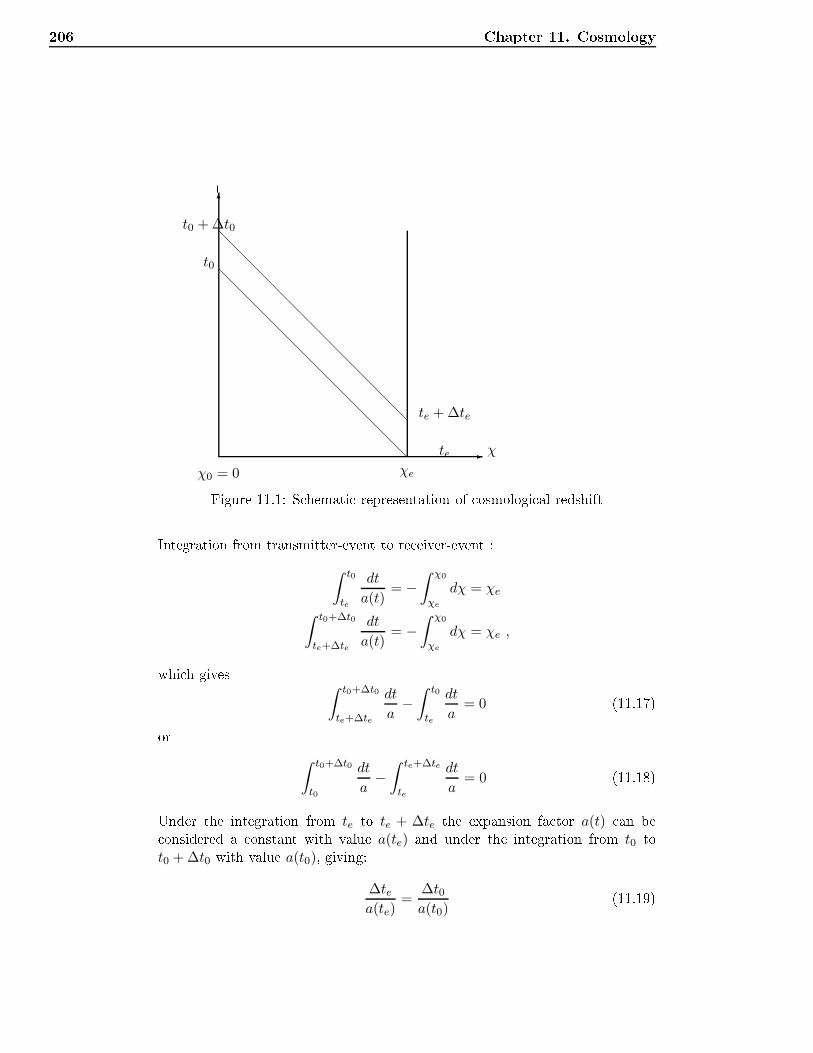
206 Chapter 11. Cosmology

-

6t

χ

t0 + ∆t0

t0

χ0 = 0 χe

te + ∆te

teFigure 11.1: S hemati representation of osmologi al redshiftIntegration from transmitter-event to re eiver-event :∫ t0

te

dt

a(t)= −

∫ χ0

χe

dχ = χe

∫ t0+∆t0

te+∆te

dt

a(t)= −

∫ χ0

χe

dχ = χe ,whi h gives ∫ t0+∆t0

te+∆te

dt

a−∫ t0

te

dt

a= 0 (11.17)or

∫ t0+∆t0

t0

dt

a−∫ te+∆te

te

dt

a= 0 (11.18)Under the integration from te to te + ∆te the expansion fa tor a(t) an be onsidered a onstant with value a(te) and under the integration from t0 to

t0 + ∆t0 with value a(t0), giving:∆tea(te)

=∆t0a(t0)

(11.19)

11.3 Cosmi dynami s 207∆t0 and ∆te are intervals of the light at the re eiving and transmitting time.Sin e the wavelength of the light is λ = c∆t we have:

λ0

a(t0)=

λea(te)

(11.20)This an be interpreted as a stret hing of the ele tromagneti waves due tothe expansion of spa e. The osmologi al redshift is denoted by z and is givenby:z =

λ0 − λeλe

=a(t0)

a(te)− 1 (11.21)Using a0 ≡ a(t0) we an write this as:

1 + z(t) =a0

a(11.22)11.3.3 Cosmi uidsThe energy-momentum tensor for a perfe t uid (no vis osity and no thermal ondu tivity) is

Tµν = (ρ+ p)uµuν + pgµν (11.23)In an orthonormal basisTµν = (ρ+ p)uµuν + pηµν (11.24)where ηµν is the Minkowski metri . We onsider 3 types of osmi uid:1. dust: p = 0,

T µν = ρuµuν (11.25)2. radiation: p = 13ρ,

T µν =4

3ρuµuν + pη µν

=ρ

3(4uµuν + η µν)

(11.26)The tra eT = T µµ =

ρ

3(4uµuµ + δµµ) = 0 (11.27)3. va uum: p = −ρ,

T µν = −ρη µν (11.28)If va uum an be des ribed as a perfe t uid we have pv = −ρv, whereρ is the energy density. It an be related to Einstein's osmologi al onstant,Λ = 8πGρv .One has also introdu ed a more general type of va uum energy given bythe equation of state pφ = wρφ, where φ denotes that the va uum energy is

208 Chapter 11. Cosmology onne ted to a s alar eld φ. In a homogeneous universe the pressure and thedensity are given bypφ =

1

2φ2 − V (φ), ρφ =

1

2φ2 + V (φ) (11.29)where V (φ) is the potential for the s alar eld. Then we have

w =12 φ

2 − V (φ)12 φ

2 + V (φ)(11.30)The spe ial ase φ = 0 gives the Lorentz invariant va uum with w = −1. Themore general va uum is alled quintessen e.11.3.4 Isotropi and homogeneous universe modelsWe will dis uss isotropi and homogenous universe models with perfe t uidand a non-vanishing osmologi al onstant Λ. Cal ulating the omponents ofthe Einstein tensor from the line-ement (11.14) we nd in an orthonormal basis

Ett =3a2

a2+

3k

a2(11.31)

Emm = −2a

a− a2

a2− k

a2. (11.32)The omponents of the energy-momentum tensor of a perfe t uid in a omovingorthonormal basis are

Ttt = ρ, Tmm = p. (11.33)Hen e the tt omponent of Einstein's eld equations is3a2 + k

a2= 8πGρ+ Λ (11.34)

mm omponents:−2

a

a− a2

a2− k

a2= 8πGp − Λ (11.35)where ρ is the energy density and p is the pressure. The equations with vanishing osmologi al onstant are alled the Friedmann equations. Inserting eq. (11.34)into eq. (11.35) gives:

a = −4πG

3a(ρ+ 3p) (11.36)If we interpret ρ as the mass density and use the speed of light c, we get

a = −4πG

3a(ρ+ 3p/c2) (11.37)Inserting the gravitational mass density ρG from eq.(10.25) this equation takesthe form

a = −4πG

3aρG (11.38)

11.3 Cosmi dynami s 209Inserting p = wρc2 into (10.25) givesρG = (1 + 3w)ρ (11.39)whi h is negative for w < −1/3, i.e. for φ2 < V (φ). Spe ial ases:

• dust: w = 0, ρG = ρ

• radiation: w = 13 , ρG = 2ρ

• Lorentz-invariant va uum: w = −1, ρG = −2ρIn a universe dominated by a Lorentz-invariant va uum the a eleration of the osmi expansion isav =

8πG

3aρv > 0, (11.40)i.e. a elerated expansion. This means that va uum a ts upon itself with repul-sive gravitation.The eld equations an be ombined into

H2 ≡(a

a

)2

=8πG

3ρm +

Λ

3− k

a2(11.41)where ρm is the density of matter, Λ = 8πGρΛ where ρΛ is the va uum energywith onstant density. ρ = ρm + ρΛ is the total mass density. Then we maywrite

H2 =8πG

3ρ− k

a2(11.42)The riti al density ρcr is the density in a universe with eu lidean spa elikegeometry, k = 0, whi h gives

ρcr =3H2

8πG(11.43)We introdu e the relative densities

Ωm =ρmρcr

, ΩΛ =ρΛ

ρcr(11.44)Furthermore we introdu e a dimensionless parameter that des ribes the urva-ture of 3-spa e

Ωk = − k

a2H2(11.45)Eq. (11.42) an now be written

Ωm + ΩΛ + Ωk = 1 (11.46)From the Bian hi identity and Einstein's eld equations follow that the energy-momentum density tensor is ovariant divergen e free. The time- omponentexpresses the equation of ontinuity and takes the form[(ρ+ p)utuν ];ν + (pηtν);ν = 0 (11.47)

210 Chapter 11. CosmologySin e ut = 1, um = 0 and ηtt = −1, ηtm = 0, we get(ρ+ p). + (ρ+ p)uν;ν − p = 0 (11.48)orρ+ (ρ+ p)(uν,ν + Γν

tν) = 0 (11.49)Here uν,ν = 0 and Γt

tt= 0. Cal ulating Γm

tmfor dωµ = Γµ

αβωα ∧ ωβ we get

Γmtm

= Γrtr

+ Γθtθ

+ Γφtφ

= 3a

a(11.50)Hen e

ρ+ 3(ρ+ p)a

a= 0 (11.51)whi h may be written

(ρa3). + p(a3). = 0 (11.52)Let V = a3 be a omoving volume in the universe and U = ρV be the energyin the omoving volume. Then we may writedU + pdV = 0 (11.53)This is the rst law of thermodynami s for an adiabati expansion. It followsthat the universe expands adiabati ally. The adiabati equation an be writtenρ

ρ+ p= −3

a

a(11.54)Assuming p = wρ we get

dρ

ρ= −3(1 + w)

da

a

lnρ

ρ0= ln

(a

a0

)−3(1+w)It follows thatρ = ρ0

(a

a0

)−3(1+w) (11.55)This equation tells how the density of dierent types of matter depends on theexpansion fa torρa3(1+w) = constant (11.56)Spe ial ases:

• dust: w = 0 gives ρda3 = constantThus, the mass in a omoving volume is onstant.

11.4 Some osmologi al models 211• radiation: w = 1

3 gives ρra4 = constantThus, the radiation energy density de reases faster than the ase with dust when the universe is expanding. The energyin a omoving volume is de reasing be ause of the thermo-dynami work on the surfa e. In a remote past, the densityof radiation must have ex eeded the density of dust:ρd0a

30 =ρda

3

ρr0a40 =ρra

4

ρra4

ρda3=ρr0a

40

ρd0a30The expansion fa tor when ρr = ρd:

a(t1) =ρr0ρd0

a0

• Lorentz-invariant va uum: w = −1 gives ρΛ = constant.The va uum energy in a omoving volume is in reasing ∝ a3.11.4 Some osmologi al models11.4.1 Radiation dominated modelThe energy-momentum tensor for radiation is tra e free. A ording to the Ein-stein eld equations the Einstein tensor must then be tra e free:aa+ a2 + k = 0

(aa+ kt)· = 0(11.57)Integration gives

aa+ kt = B (11.58)Another integration gives1

2a2 +

1

2kt2 = Bt+C (11.59)The initial ondition a(0) = 0 gives C = 0. Hen e

a =√

2Bt− kt2 (11.60)For k = 0 we havea =

√2Bt , a =

√B

2t(11.61)The expansion velo ity rea hes innity at t = 0, (limt→0 a = ∞)

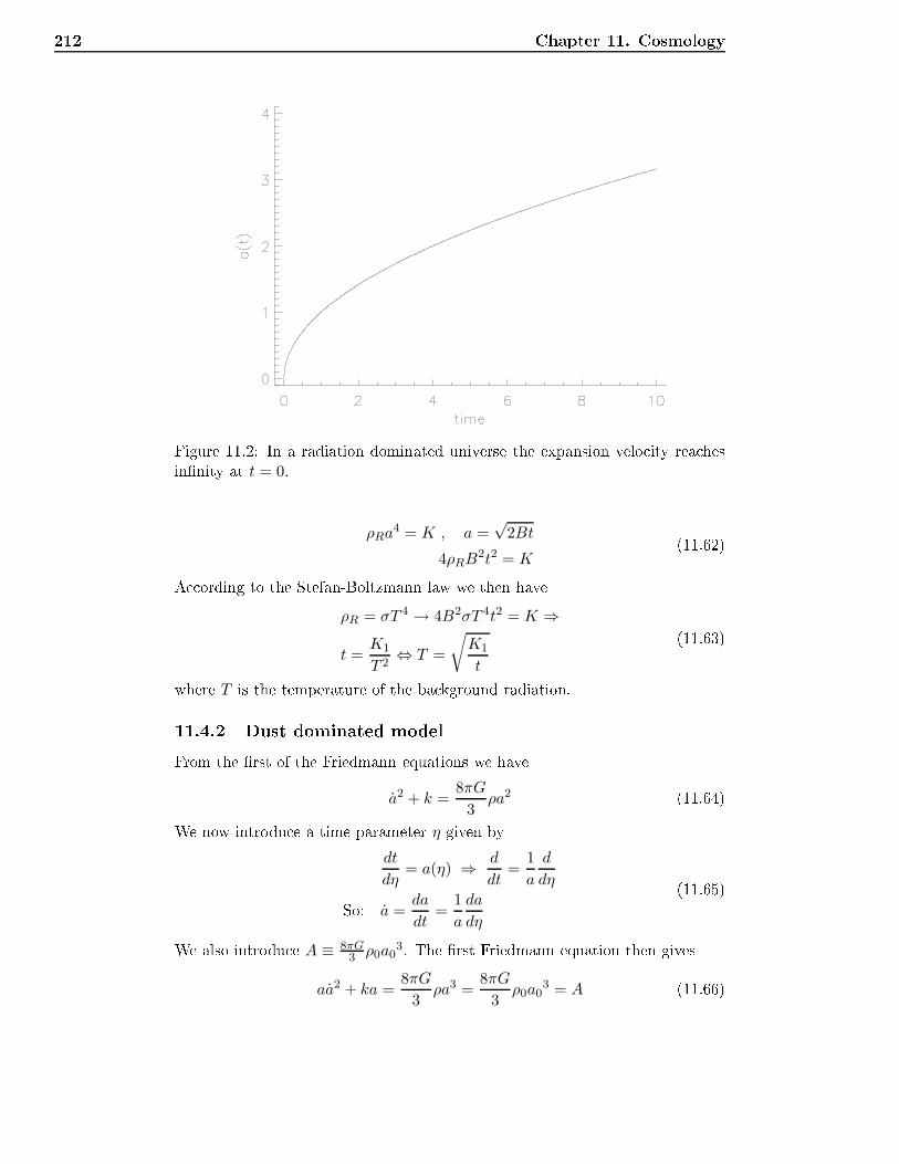
212 Chapter 11. Cosmology

Figure 11.2: In a radiation dominated universe the expansion velo ity rea hesinnity at t = 0.ρRa

4 = K , a =√

2Bt

4ρRB2t2 = K

(11.62)A ording to the Stefan-Boltzmann law we then haveρR = σT 4 → 4B2σT 4t2 = K ⇒

t =K1

T 2⇔ T =

√K1

t

(11.63)where T is the temperature of the ba kground radiation.11.4.2 Dust dominated modelFrom the rst of the Friedmann equations we havea2 + k =

8πG

3ρa2 (11.64)We now introdu e a time parameter η given by

dt

dη= a(η) ⇒ d

dt=

1

a

d

dηSo: a =da

dt=

1

a

da

dη

(11.65)We also introdu e A ≡ 8πG3 ρ0a0

3. The rst Friedmann equation then givesaa2 + ka =

8πG

3ρa3 =

8πG

3ρ0a0

3 = A (11.66)

11.4 Some osmologi al models 213Using η we get1

a(da

dη)2 = A− ka

1

a2(da

dη)2 =

A

a− k

1

a

da

dη=

√A

a− k =

√A

a

√1 − a

Ak

(11.67)where we hose the positive root. We now introdu e u, given by a = Au2, u =√

aA . We then get

da

dη= 2Au

du

dη(11.68)whi h together with the equation above give

1

Au22Au

du

dη=

1

u

√1 − ku2

⇓du√

1 − ku2=

1

2dη

(11.69)This equation will rst be integrated for k < 0. Then k = −|k|, so that∫

du√1 + |k|u2

=η

2+K (11.70)or ar sinh(√−ku) = η

2 +K. The ondition u(0) = 0 gives K = 0. Hen e− k

Aa = sinh2 η

2=

1

2(cosh η − 1) (11.71)or

a = − A

2k(cosh η − 1) (11.72)From eqs. (11.43), (11.44) and (11.66) we have

A =8πG

3ρm0 = H2

0

ρm0

ρcr0= H2

0Ωm0 (11.73)From egs. (11.45) and (11.46) we getk = H2

0 (Ωm0 − 1) (11.74)Hen e, the s ale fa tor of the negatively urved, dust dominated universe modelisa(η) =

1

2

Ωm0

1 − Ωm0(cosh η − 1) (11.75)

214 Chapter 11. CosmologyInserting this into eq. (11.65) and integrating with t(0) = η(0) leads tot(η) =

Ωm0

2H0(1 − Ωm0)3/2(sinh η − η) (11.76)Integrating eg. (11.69) for k = 0 leads to an Einstein-deSitter universe

a(t) = (t

t0)

23 (11.77)Finally integrating eg. (11.69) for k > 0 gives, in a similar way as for k < 0

a(η) =1

2

Ωm0

Ωm0 − 1(1 − cos η) (11.78)

t(η) =Ωm0

2H0(Ωm0 − 1)3/2(η − sin η) (11.79)We see that this is a parametri representation of a y loid.In the Einstein-deSitter model the Hubble fa tor is

H =a

a=

2

3

1

t, t =

2

3

1

H=

2

3tH (11.80)The riti al density in the Einstein-deSitter model is given by the rst Fried-mann equation:

H2 =8πG

3ρ r , k = 0

⇓

ρ r =3H2

8πG, Ω =

ρ

ρ r (11.81)Example 11.4.1 (Age-redshift relation for dust dominated universe with k = 0)

1 + z =a0

a⇒ a =

a0

1 + z

da = − a0

(1 + z)2dz = − a

1 + zdz

(11.82)Eq. (11.34) gives( aa

)2=

8πG

3ρ =

8πG

3

ρ0a30

a3

=8πG

3ρ0(1 + z)3

(11.83)

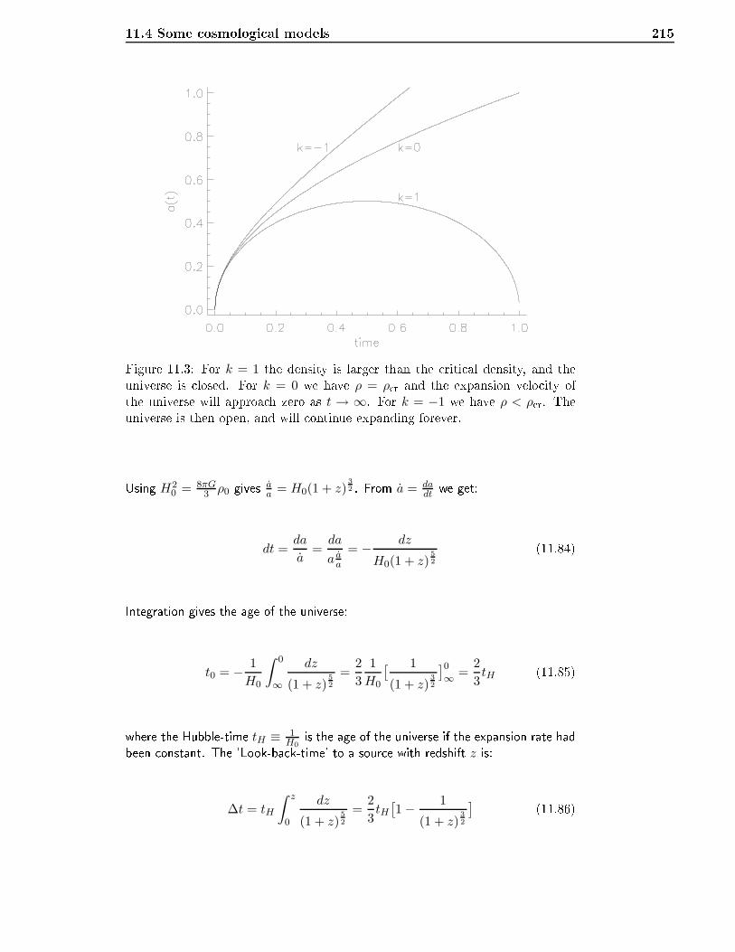
11.4 Some osmologi al models 215

Figure 11.3: For k = 1 the density is larger than the riti al density, and theuniverse is losed. For k = 0 we have ρ = ρ r and the expansion velo ity ofthe universe will approa h zero as t → ∞. For k = −1 we have ρ < ρ r. Theuniverse is then open, and will ontinue expanding forever.Using H20 = 8πG

3 ρ0 gives aa = H0(1 + z)

32 . From a = da

dt we get:dt =

da

a=da

a aa= − dz

H0(1 + z)52

(11.84)Integration gives the age of the universe:t0 = − 1

H0

∫ 0

∞

dz

(1 + z)52

=2

3

1

H0

[ 1

(1 + z)32

]0∞ =

2

3tH (11.85)where the Hubble-time tH ≡ 1

H0is the age of the universe if the expansion rate hadbeen onstant. The 'Look-ba k-time' to a sour e with redshift z is:

∆t = tH

∫ z

0

dz

(1 + z)52

=2

3tH[1 − 1

(1 + z)32

] (11.86)

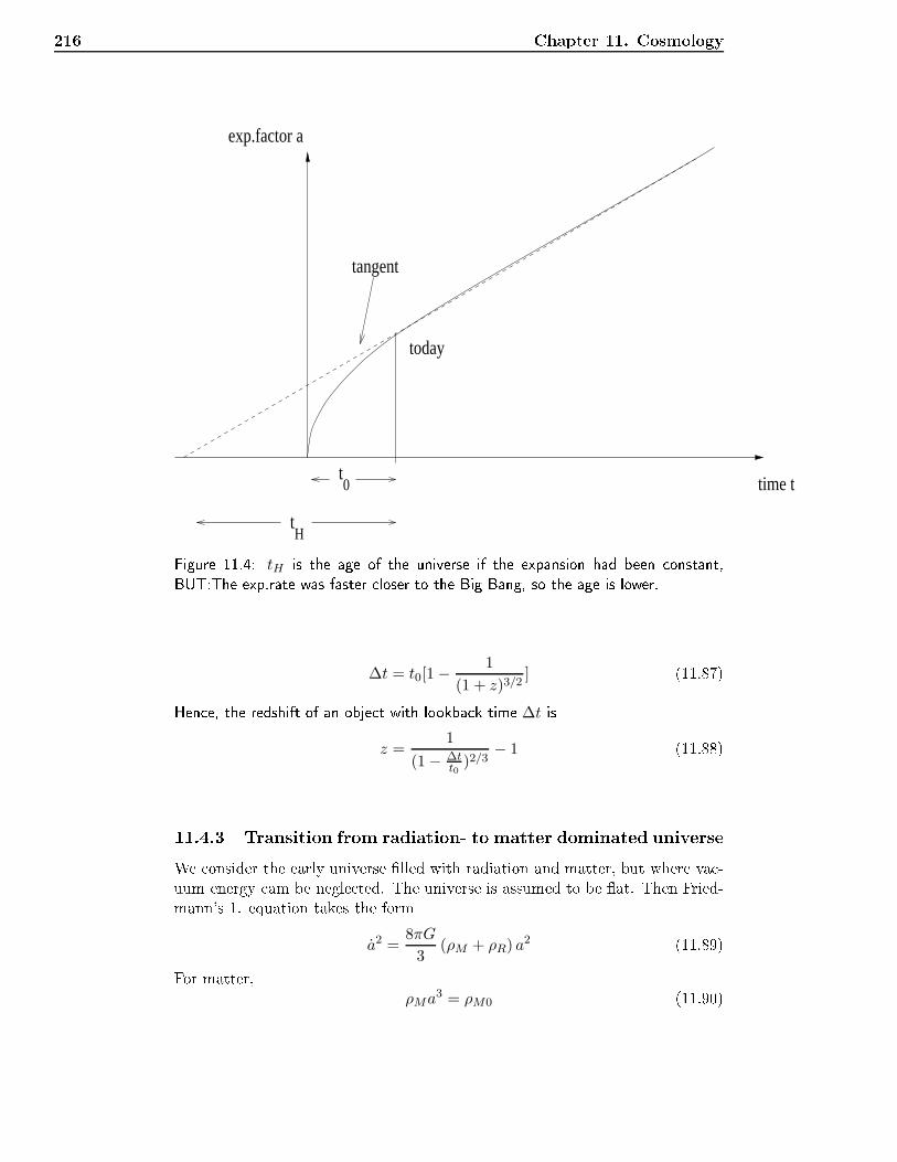
216 Chapter 11. Cosmology

tangent

time t

exp.factor a

t0

tH

today

Figure 11.4: tH is the age of the universe if the expansion had been onstant,BUT:The exp.rate was faster loser to the Big Bang, so the age is lower.∆t = t0[1 − 1

(1 + z)3/2] (11.87)Hen e, the redshift of an obje t with lookba k time ∆t is

z =1

(1 − ∆tt0

)2/3− 1 (11.88)

11.4.3 Transition from radiation- to matter dominated universeWe onsider the early universe lled with radiation and matter, but where va -uum energy am be negle ted. The universe is assumed to be at. Then Fried-mann's 1. equation takes the forma2 =

8πG

3(ρM + ρR) a2 (11.89)For matter,

ρMa3 = ρM0 (11.90)

11.4 Some osmologi al models 217For radiation,ρRa

4 = ρR0 (11.91)Hen ea2a2 =

8πG

3(ρM0 a+ ρR0) (11.92)The present values of the riti al density and the density parameters are

ρcr0 =3H2

0

8πG(11.93)

ΩM0 =ρM0

ρcr0(11.94)

ΩR0 =ρR0

ρcr0(11.95)giving

aa = H0 (ΩM0 a+ ΩR0)1/2 (11.96)Integration with a(0) = 0 leads to

H0t =4

3

Ω3/2R0

Ω2M0

+2

3

(ΩM0 a− 2ΩR0) (ΩM0 a+ ΩR0)1/2

Ω2M0

(11.97)From eqs. (11.90) and (11.91) follows that at the transition time teq whenρM = ρR, the s ale fa tor has the value

aeq =ρR0

ρM0=

ΩR0

ΩM0(11.98)Inserting this into eq. (11.97) gives

teq =2

3

(2 −

√2) Ω

3/2R0

Ω2M0

tH (11.99)The mi rowave ba kground radiation has a temperature 2,73 K orrespondingto a density parameter ΩR0 = 8, 4 · 10−5. In a at universe without va uumenergy ΩM0 = 1 − ΩR0. From the value of H0 as determined by measurementswe have tH ≈ 14 · 109 years. This leads to teq = 47 · 103 years.11.4.4 Friedmann-Lemaître modelThe dynami s of galaxies and lusters of galaxies has made it lear that farstronger gravitational elds are needed to explain the observed motions thanthose produ ed by visible matter (M Gaugh 2001). At the same time it hasbe ome lear that the density of this dark matter is only about 30% of the riti aldensity, although it is a predi tion by the usual versions of the inationaryuniverse models that the density ought to be equal to the riti al density (Linde2001). Also the re ent observations of the temperature u tuations of the osmi mi rowave radiation have shown that spa e is either at or very lose to at(Bernadis et.al 2001, Stompor et al. 2001, Pryke et al. 2001). The energy that

218 Chapter 11. Cosmologylls up to the riti al density must be evenly distributed in order not to ae tthe dynami s of the galaxies and the lusters.Furthermore, about two years ago observations of supernovae of type Ia withhigh osmi red shifts indi ated that the expansion of the universe is a elerating(Riess et al. 1998, Perlmutter et al. 1999). This was explained as a result ofrepulsive gravitation due to some sort of va uum energy. Thereby the missingenergy needed to make spa e at, was identied as va uum energy. Hen e, itseems that we live in a at universe with va uum energy having a density around70% of the riti al density and with matter having a density around 30% of the riti al density.Until the dis overy of the a elerated expansion of the universe the standardmodel of the universe was assumed to be the Einstein-DeSitter model, whi h isa at universe model dominated by old matter. This universe model is thor-oughly presented in nearly every text book on general relativity and osmology.Now it seems that we must repla e this model with a new "standard model" ontaining both dark matter and va uum energy.Re ently several types of va uum energy or so alled quintessen e energyhave been dis ussed (Zlatev, Wang and Steinhardt 1999, Carroll 1998). How-ever, the most simple type of va uum energy is the Lorentz invariant va uumenergy (LIVE), whi h has onstant energy density during the expansion of theuniverse (Zeldovi h 1968, Grøn 1986). This type of energy an be mathemati- ally represented by in luding a osmologi al onstant in Einstein's gravitationaleld equations. The at universe model with old dark matter and this type ofva uum energy is the Friedmann-Lemaître model.The eld equations for the at Friedmann-Lemaître is found by puttingk = p = 0 in equation (11.35). This gives

2a

a+a2

a2= Λ (11.100)Integration leads to

aa2 =Λ

3a3 +K (11.101)where K is a onstant of integration. Sin e the amount of matter in a volume omoving with the osmi expansion is onstant, ρMa3 = ρM0a

30, where theindex 0 refers to measured values at the present time. Normalizing the expansionfa tor so that a0 = 1 and omparing eqs.(11.42) and(11.101) then gives K =

(8πG/3)ρM0. Introdu ing a new variable x by a3 = x2 and integrating on emore with the initial ondition a(0) = 0 we obtaina3 =

3K

Λsinh2

(t

tΛ

), tΛ =

2√3Λ

(11.102)The va uum energy has a onstant density ρΛ given byΛ = 8πGρΛ (11.103)The riti al density, whi h is the density making the 3-spa e of the universe at,isρcr =

3H2

8πG(11.104)

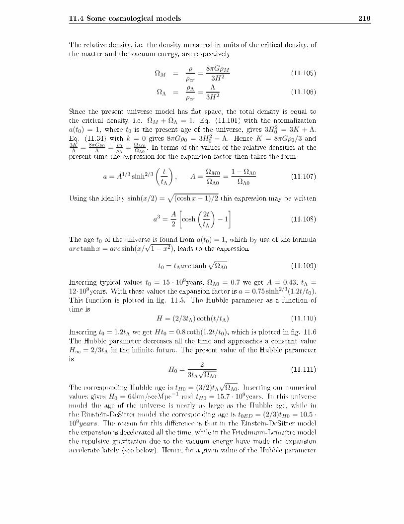
11.4 Some osmologi al models 219The relative density, i.e. the density measured in units of the riti al density, ofthe matter and the va uum energy, are respe tivelyΩM =

ρ

ρcr=

8πGρM3H2

(11.105)ΩΛ =

ρΛ

ρcr=

Λ

3H2(11.106)Sin e the present universe model has at spa e, the total density is equal tothe riti al density, i.e. ΩM + ΩΛ = 1. Eq. (11.101) with the normalization

a(t0) = 1, where t0 is the present age of the universe, gives 3H20 = 3K + Λ.Eq. (11.34) with k = 0 gives 8πGρ0 = 3H2

0 − Λ. Hen e K = 8πGρ0/3 and3KΛ = 8πGρ0

Λ = ρ0ρΛ

= ΩM0ΩΛ0

. In terms of the values of the relative densities at thepresent time the expression for the expansion fa tor then takes the forma = A1/3 sinh2/3

(t

tΛ

), A =

ΩM0

ΩΛ0=

1 − ΩΛ0

ΩΛ0(11.107)Using the identity sinh(x/2) =

√(coshx− 1)/2 this expression may be written

a3 =A

2

[cosh

(2t

tΛ

)− 1

] (11.108)The age t0 of the universe is found from a(t0) = 1, whi h by use of the formulaarc tanhx = arc sinh(x/

√1 − x2), leads to the expressiont0 = tΛarc tanh

√ΩΛ0 (11.109)Inserting typi al values t0 = 15 · 109years, ΩΛ0 = 0.7 we get A = 0.43, tΛ =

12·109years. With these values the expansion fa tor is a = 0.75 sinh2/3(1.2t/t0).This fun tion is plotted in g. 11.5. The Hubble parameter as a fun tion oftime isH = (2/3tΛ) coth(t/tΛ) (11.110)Inserting t0 = 1.2tΛ we get Ht0 = 0.8 coth(1.2t/t0), whi h is plotted in g. 11.6The Hubble parameter de reases all the time and approa hes a onstant value

H∞ = 2/3tΛ in the innite future. The present value of the Hubble parameterisH0 =

2

3tΛ√

ΩΛ0(11.111)The orresponding Hubble age is tH0 = (3/2)tΛ

√ΩΛ0. Inserting our numeri alvalues gives H0 = 64km/se Mp −1 and tH0 = 15.7 · 109years. In this universemodel the age of the universe is nearly as large as the Hubble age, while inthe Einstein-DeSitter model the orresponding age is t0ED = (2/3)tH0 = 10.5 ·

109years. The reason for this dieren e is that in the Einstein-DeSitter modelthe expansion is de elerated all the time, while in the Friedmann-Lemaître modelthe repulsive gravitation due to the va uum energy have made the expansiona elerate lately (see below). Hen e, for a given value of the Hubble parameter

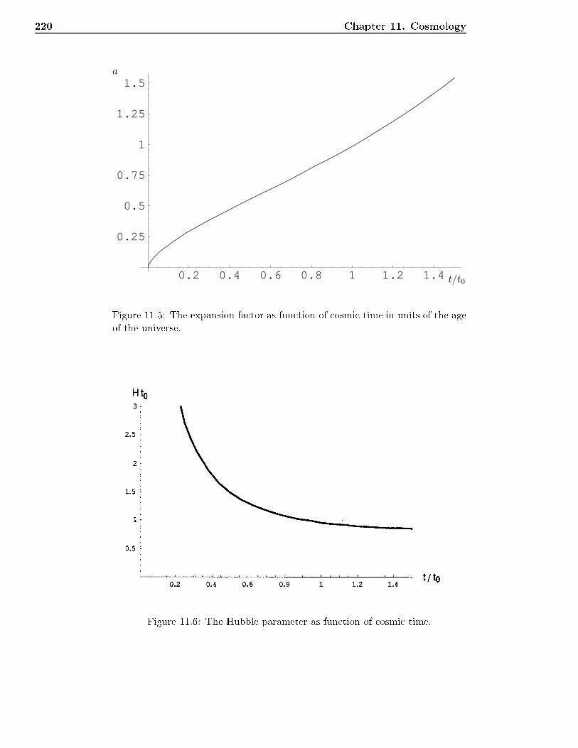
220 Chapter 11. Cosmologya

t/t00.2 0.4 0.6 0.8 1 1.2 1.4

0.25

0.5

0.75

1

1.25

1.5

Figure 11.5: The expansion fa tor as fun tion of osmi time in units of the ageof the universe.

Figure 11.6: The Hubble parameter as fun tion of osmi time.

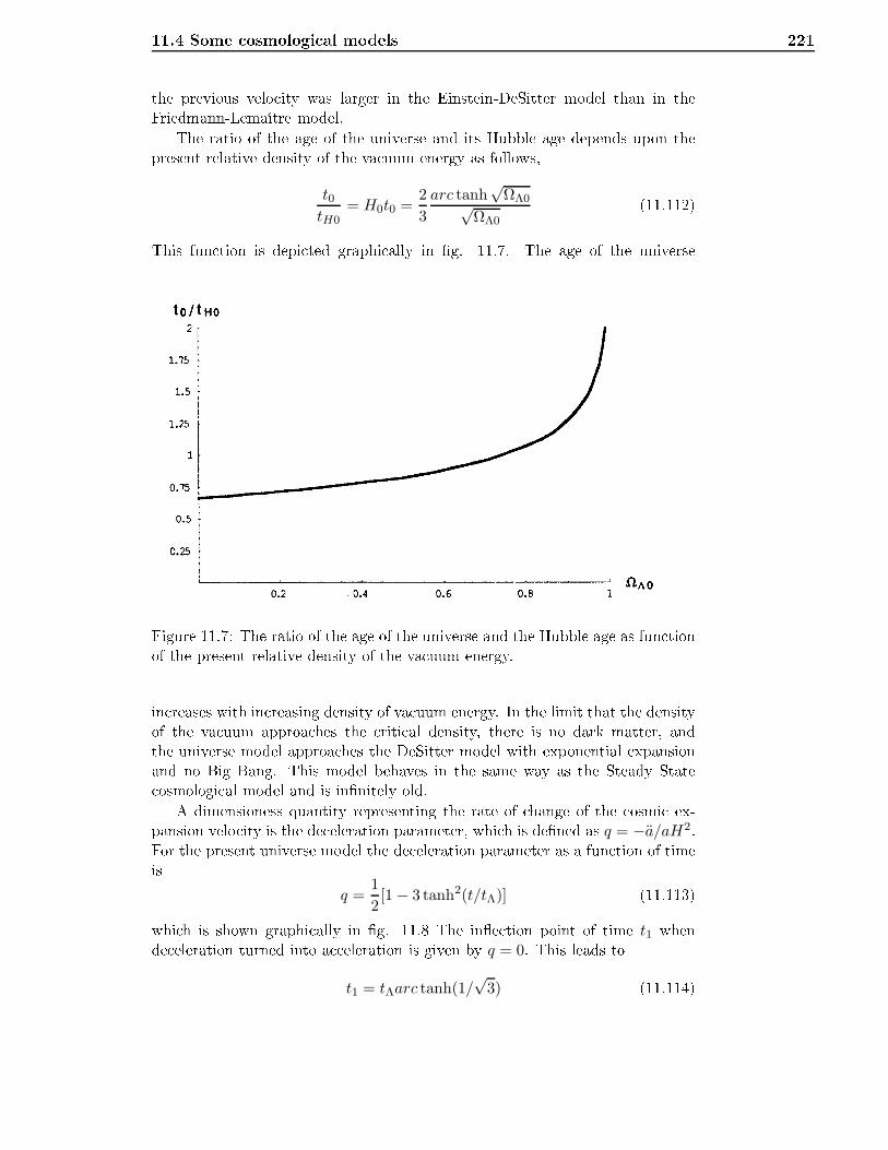
11.4 Some osmologi al models 221the previous velo ity was larger in the Einstein-DeSitter model than in theFriedmann-Lemaître model.The ratio of the age of the universe and its Hubble age depends upon thepresent relative density of the va uum energy as follows,t0tH0

= H0t0 =2

3

arc tanh√

ΩΛ0√ΩΛ0

(11.112)This fun tion is depi ted graphi ally in g. 11.7. The age of the universe

Figure 11.7: The ratio of the age of the universe and the Hubble age as fun tionof the present relative density of the va uum energy.in reases with in reasing density of va uum energy. In the limit that the densityof the va uum approa hes the riti al density, there is no dark matter, andthe universe model approa hes the DeSitter model with exponential expansionand no Big Bang. This model behaves in the same way as the Steady State osmologi al model and is innitely old.A dimensioness quantity representing the rate of hange of the osmi ex-pansion velo ity is the de eleration parameter, whi h is dened as q = −a/aH2.For the present universe model the de eleration parameter as a fun tion of timeisq =

1

2[1 − 3 tanh2(t/tΛ)] (11.113)whi h is shown graphi ally in g. 11.8 The ine tion point of time t1 whende eleration turned into a eleration is given by q = 0. This leads to

t1 = tΛarc tanh(1/√

3) (11.114)

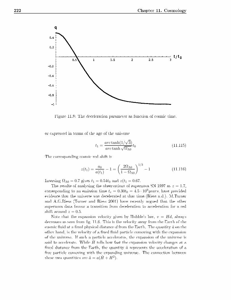
222 Chapter 11. Cosmology

Figure 11.8: The de eleration parameter as fun tion of osmi time.or expressed in terms of the age of the universet1 =

arc tanh(1/√

3)

arc tanh√

ΩΛ0t0 (11.115)The orresponding osmi red shift is

z(t1) =a0

a(t1)− 1 =

(2ΩΛ0

1 − ΩΛ0

)1/3

− 1 (11.116)Inserting ΩΛ0 = 0.7 gives t1 = 0.54t0 and z(t1 = 0.67.The results of analysing the observations of supernova SN 1997 at z = 1.7, orresponding to an emission time te = 0.30t0 = 4.5 · 109years, have providedeviden e that the universe was de elerated at that time (Riess n.d.). M.Turnerand A.G.Riess (Turner and Riess 2001) have re ently argued that the othersupernova data favour a transition from de eleration to a eleration for a redshift around z = 0.5.Note that the expansion velo ity given by Hubble's law, v = Hd, alwaysde reases as seen from g. 11.6. This is the velo ity away from the Earth of the osmi uid at a xed physi al distan e d from the Earth. The quantity a on theother hand, is the velo ity of a xed uid parti le omoving with the expansionof the universe. If su h a parti le a elerates, the expansion of the universe issaid to a elerate. While H tells how fast the expansion velo ity hanges at axed distan e from the Earth, the quantity a represents the a eleration of afree parti le omoving with the expanding universe. The onne tion betweenthese two quantities are a = a(H +H2).

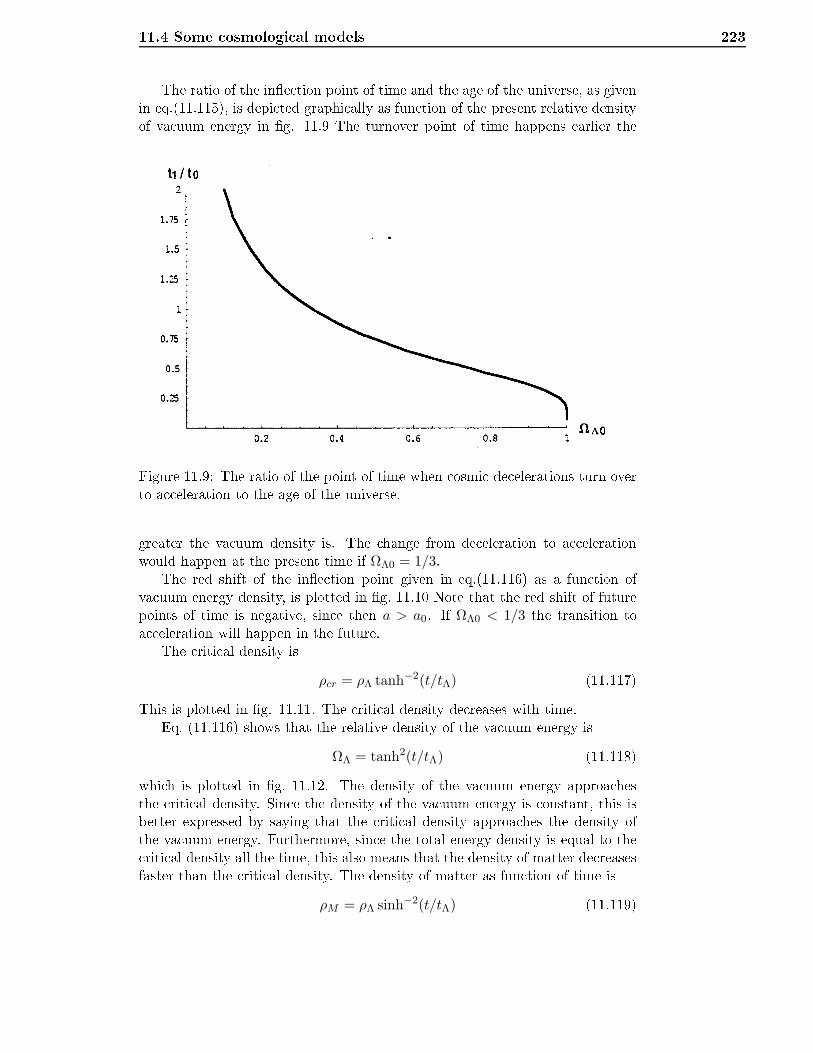
11.4 Some osmologi al models 223The ratio of the ine tion point of time and the age of the universe, as givenin eq.(11.115), is depi ted graphi ally as fun tion of the present relative densityof va uum energy in g. 11.9 The turnover point of time happens earlier the

Figure 11.9: The ratio of the point of time when osmi de elerations turn overto a eleration to the age of the universe.greater the va uum density is. The hange from de eleration to a elerationwould happen at the present time if ΩΛ0 = 1/3.The red shift of the ine tion point given in eq.(11.116) as a fun tion ofva uum energy density, is plotted in g. 11.10 Note that the red shift of futurepoints of time is negative, sin e then a > a0. If ΩΛ0 < 1/3 the transition toa eleration will happen in the future.The riti al density isρcr = ρΛ tanh−2(t/tΛ) (11.117)This is plotted in g. 11.11. The riti al density de reases with time.Eq. (11.116) shows that the relative density of the va uum energy is

ΩΛ = tanh2(t/tΛ) (11.118)whi h is plotted in g. 11.12. The density of the va uum energy approa hesthe riti al density. Sin e the density of the va uum energy is onstant, this isbetter expressed by saying that the riti al density approa hes the density ofthe va uum energy. Furthermore, sin e the total energy density is equal to the riti al density all the time, this also means that the density of matter de reasesfaster than the riti al density. The density of matter as fun tion of time isρM = ρΛ sinh−2(t/tΛ) (11.119)

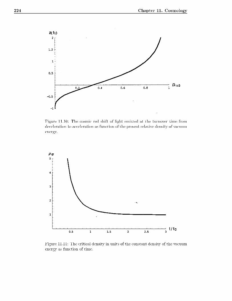
224 Chapter 11. Cosmology

Figure 11.10: The osmi red shift of light emitted at the turnover time fromde eleration to a eleration as fun tion of the present relative density of va uumenergy.

Figure 11.11: The riti al density in units of the onstant density of the va uumenergy as fun tion of time.

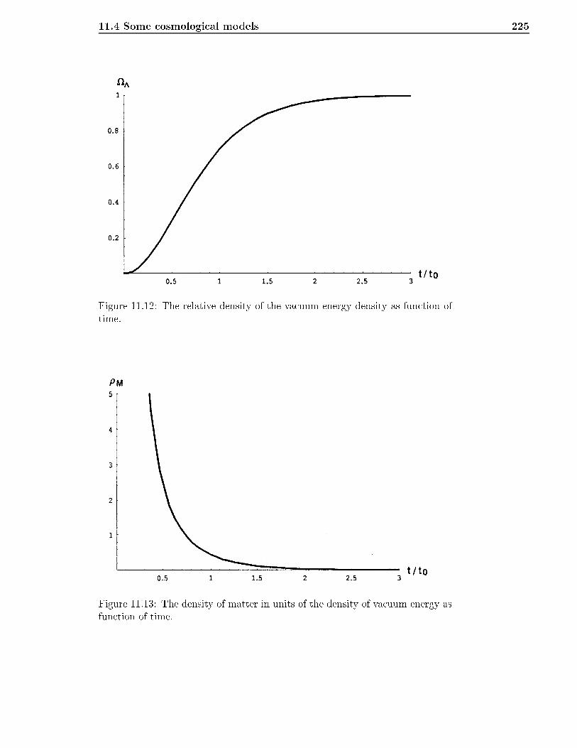
11.4 Some osmologi al models 225

Figure 11.12: The relative density of the va uum energy density as fun tion oftime.

Figure 11.13: The density of matter in units of the density of va uum energy asfun tion of time.

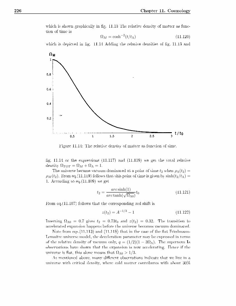
226 Chapter 11. Cosmologywhi h is shown graphi ally in g. 11.13 The relative density of matter as fun -tion of time isΩM = cosh−2(t/tΛ) (11.120)whi h is depi ted in g. 11.14 Adding the relative densities of g. 11.13 and

Figure 11.14: The relative density of matter as fun tion of time.g. 11.14 or the expressions (11.117) and (11.119) we get the total relativedensity ΩTOT = ΩM + ΩΛ = 1.The universe be ame va uum dominated at a point of time t2 when ρΛ(t2) =ρM (t2). From eq.(11.119) follows that this point of time is given by sinh(t2/tΛ) =1. A ording to eq.(11.109) we get

t2 =arc sinh(1)

arc tanh(√

ΩΛ0)t0 (11.121)From eq.(11.107) follows that the orresponding red shift is

z(t2) = A−1/3 − 1 (11.122)Inserting ΩΛ0 = 0.7 gives t2 = 0.73t0 and z(t2) = 0.32. The transition toa elerated expansion happens before the universe be omes va uum dominated.Note from eqs.(11.113) and (11.118) that in the ase of the at Friedmann-Lemaître universe model, the de eleration parameter may be expressed in termsof the relative density of va uum only, q = (1/2)(1 − 3ΩΛ). The supernova Iaobservations have shown that the expansion is now a elerating. Hen e if theuniverse is at, this alone means that ΩΛ0 > 1/3.As mentioned above, many dierent observations indi ate that we live in auniverse with riti al density, where old matter ontributes with about 30%

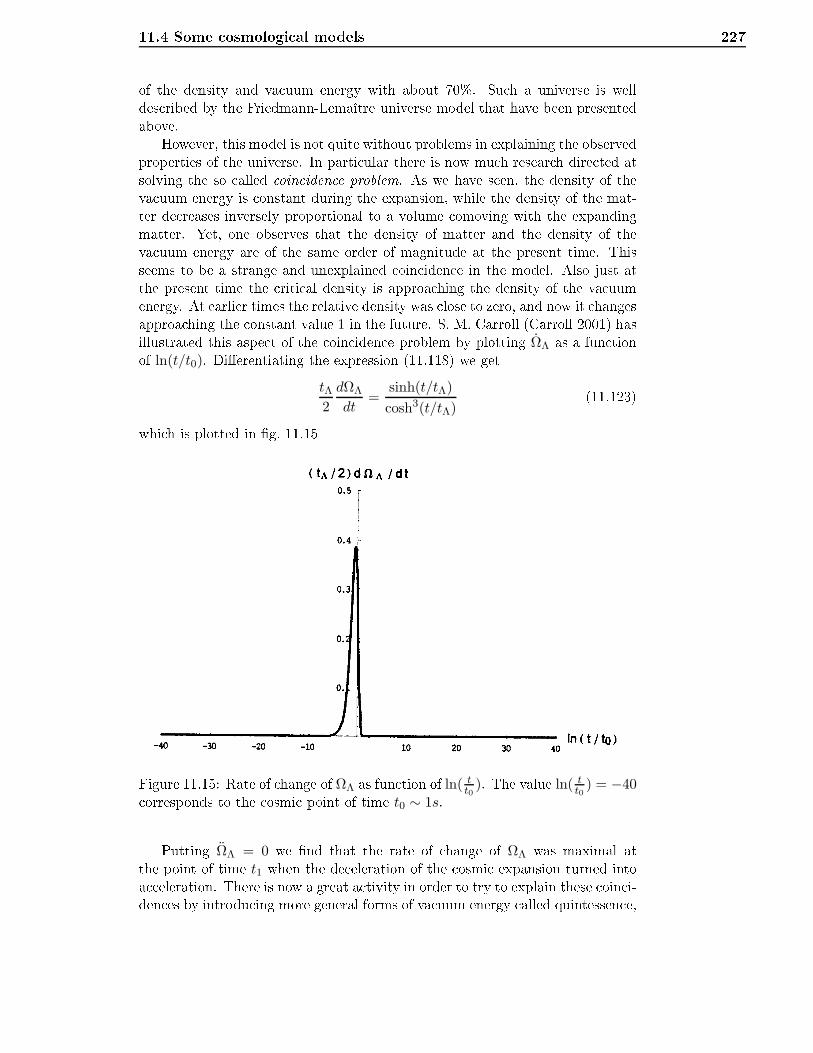
11.4 Some osmologi al models 227of the density and va uum energy with about 70%. Su h a universe is welldes ribed by the Friedmann-Lemaître universe model that have been presentedabove.However, this model is not quite without problems in explaining the observedproperties of the universe. In parti ular there is now mu h resear h dire ted atsolving the so alled oin iden e problem. As we have seen, the density of theva uum energy is onstant during the expansion, while the density of the mat-ter de reases inversely proportional to a volume omoving with the expandingmatter. Yet, one observes that the density of matter and the density of theva uum energy are of the same order of magnitude at the present time. Thisseems to be a strange and unexplained oin iden e in the model. Also just atthe present time the riti al density is approa hing the density of the va uumenergy. At earlier times the relative density was lose to zero, and now it hangesapproa hing the onstant value 1 in the future. S. M. Carroll (Carroll 2001) hasillustrated this aspe t of the oin iden e problem by plotting ΩΛ as a fun tionof ln(t/t0). Dierentiating the expression (11.118) we gettΛ2

dΩΛ

dt=

sinh(t/tΛ)

cosh3(t/tΛ)(11.123)whi h is plotted in g. 11.15

Figure 11.15: Rate of hange of ΩΛ as fun tion of ln( tt0 ). The value ln( tt0 ) = −40 orresponds to the osmi point of time t0 ∼ 1s.Putting ΩΛ = 0 we nd that the rate of hange of ΩΛ was maximal atthe point of time t1 when the de eleration of the osmi expansion turned intoa eleration. There is now a great a tivity in order to try to explain these oin i-den es by introdu ing more general forms of va uum energy alled quintessen e,

228 Chapter 11. Cosmologyand with a density determined dynami ally by the evolution of a s alar eld(Turner 2001).However, the simplest type of va uum energy is the LIVE. One may hopethat a future theory of quantum gravity may settle the matter and let us un-derstand the va uum energy. In the meantime we an learn mu h about thedynami s of a va uum dominated universe by studying simple and beautifuluniverse models su h as the Friedmann-Lemaître model.11.5 Inationary Cosmology11.5.1 Problems with the Big Bang ModelsThe Horizon ProblemThe Cosmi Mi rowave Ba kground (CMB) radiation from two points A and Bin opposite dire tions has the same temperature. This means that it has beenradiated by sour es of the same temperature in these points. Thus, the universemust have been in thermi equilibrium at the de oupling time, td = 3 ·105years.This implies that points A and B, at opposite sides of the universe, had beenin ausal onta t already at that time. I.e., a light signal must have had time tomove from A to B during the time from t = 0 to t = 3 · 105 years. The pointsA and B must have been within ea h other's horizons at the de oupling.Consider a photon moving radially in spa e des ibed by the Robertson-Walker metri (11.14) with k = 0. Light follows a null geodesi urve, i.e. the urve is dened by ds2 = 0. We get

dr =dt

a(t). (11.124)The oordinate distan e the photon has moved during the time t is

∆r =

∫ t

0

dt

a(t). (11.125)The physi al distan e the light has moved at the time t is alled the horizondistan e, and is

lh = a(t)∆r = a(t)

∫ t

0

dt

a(t). (11.126)To nd a quantitative expression for the horizon problem, we may onsidera model with riti al mass density (Eu lidian spa elike geometry.) Using p = wρand Ω = 1, integration of equation (11.36) gives

a ∝ t2

3+3w . (11.127)Inserting this into the expression for lh and integrating giveslh =

3w + 3

3w + 1t. (11.128)

11.5 Inationary Cosmology 229Let us all the volume inside the horizon the horizon volume and denote it byVH . From equation (11.128) follows that VH ∝ t3. At the de oupling time, thehorizon volume may therefore be written

(VH)d =

(tdt0

)3

V0, (11.129)where V0 is the size of the present horizon volume. Events within this volumeare ausally onne ted, and a volume of this size may be in thermal equilibriumat the de oupling time.Let (V0)d be the size, at the de oupling, of the part of the universe that orresponds to the present horizon volume, i.e. the observable universe. For ourEu lidean universe, the equation (11.127) holds, giving(V0)d =

a3(td)

a3(t0)V0 =

(tdt0

) 2w+1

V0. (11.130)From equations (11.129) and (11.130), we get(V0)d(VH)d

=

(tdt0

) 3w+1w+1

. (11.131)Using that td = 10−4t0 and inserting w = 0 for dust, we nd V0)d

(VH)d= 104.Thus, there was room for 104 ausally onne ted areas at the de oupling timewithin what presently represents our observable universe. Points at oppositesides of our observable universe were therefore not ausally onne ted at thede oupling, a ording to the Friedmann models of the universe. These models an therefore not explain that the temperature of the radiation from su h pointsis the same.The Flatness ProblemA ording to eq. (11.42), the total mass parameter Ω = ρ

ρcris given by

Ω − 1 =k

a2. (11.132)By using the expansion fa tor (11.127) for a universe near riti al massdensity, we get

Ω − 1

Ω0 − 1=

(t

t0

)2( 3w+13w+3)

. (11.133)For a radiation dominated universe, we getΩ − 1

Ω0 − 1=

t

t0. (11.134)Measurements indi ate that Ω0 − 1 is of order of magnitude 1. The age ofthe universe is about t0 = 1017s. When we stipulate initial onditions for the

230 Chapter 11. Cosmologyuniverse, it is natural to onsider the Plan k time, tP = 10−43s, sin e this isthe limit to the validity of general relativity. At earlier time, quantum ee tswill be important, and one an not give a reliable des ription without usingquantum gravitation. The stipulated initial ondition for the mass parameterthen be omes that Ω− 1 is of order 10−60 at the Plan k time. Su h an extremene tuning of the initial value of the universe's mass density an not be explainedwithin standard Big Bang osmology.Other ProblemsThe Friedman models an not explain questions about why the universe is nearlyhomogeneous and has an isotropi expansion, nor say anything about why theuniverse is expanding.11.5.2 Cosmi InationSpontaneous Symmetry Breaking and the Higgs Me hanismThe parti les responsible for the ele troweak for e, W± and Z0 are massive( ausing the weak for e to only have short distan e ee ts). This was originallya problem for the quantum eld theory des ribing this for e, sin e it made itdi ult to reate a renormalisable theory1. This was solved by Higgs and Kibblein 1964 by introdu ing the so- alled Higgs me hanism.The main idea is that the massive bosons W± and Z0 are given a mass byintera ting with a Higgs eld φ. The ee t auses the mass of the parti les to beproportional to the value of the Higgs eld in va uum. It is therefore ne essaryfor the me hanism that the Higgs eld has a value dierent from zero in theva uum (the va uum expe tation value must be non-zero).Let us see how the Higgs eld an get a non-zero va uum expe tation value.The important thing for our purpose is that the potential for the Higgs eldmay be temperature dependent. Let us assume that the potential for the Higgseld is des ribed by the fun tionV (φ) =

1

2µ2φ2 +

1

4λφ4, (11.135)where the sign of µ2 depends on whether the temperature is above or below a riti al temperature Tc. This sign has an important onsequen e for the shapeof the potential V . The potential is shown in gure 11.16 for two dierenttemperatures. For T > Tc, µ2 > 0, and the shape is like in g. 11.16(a), andthere is a stable minimum for φ = 0. However, for T < Tc, µ2 < 0, and theshape is like in g. 11.16(b). In this ase the potential has stable minima for

φ = ±φ0 = ± |µ|√λand an unstable maximum at φ = 0. For both ases, thepotential V (φ) is invariant under the symmetry transformation φ 7→ −φ (i.e.

V (φ) = V (−φ)).1The problem is that the Lagrangian for the gauge bosons an not in lude terms like m2W 2µ ,whi h are not gauge invariant

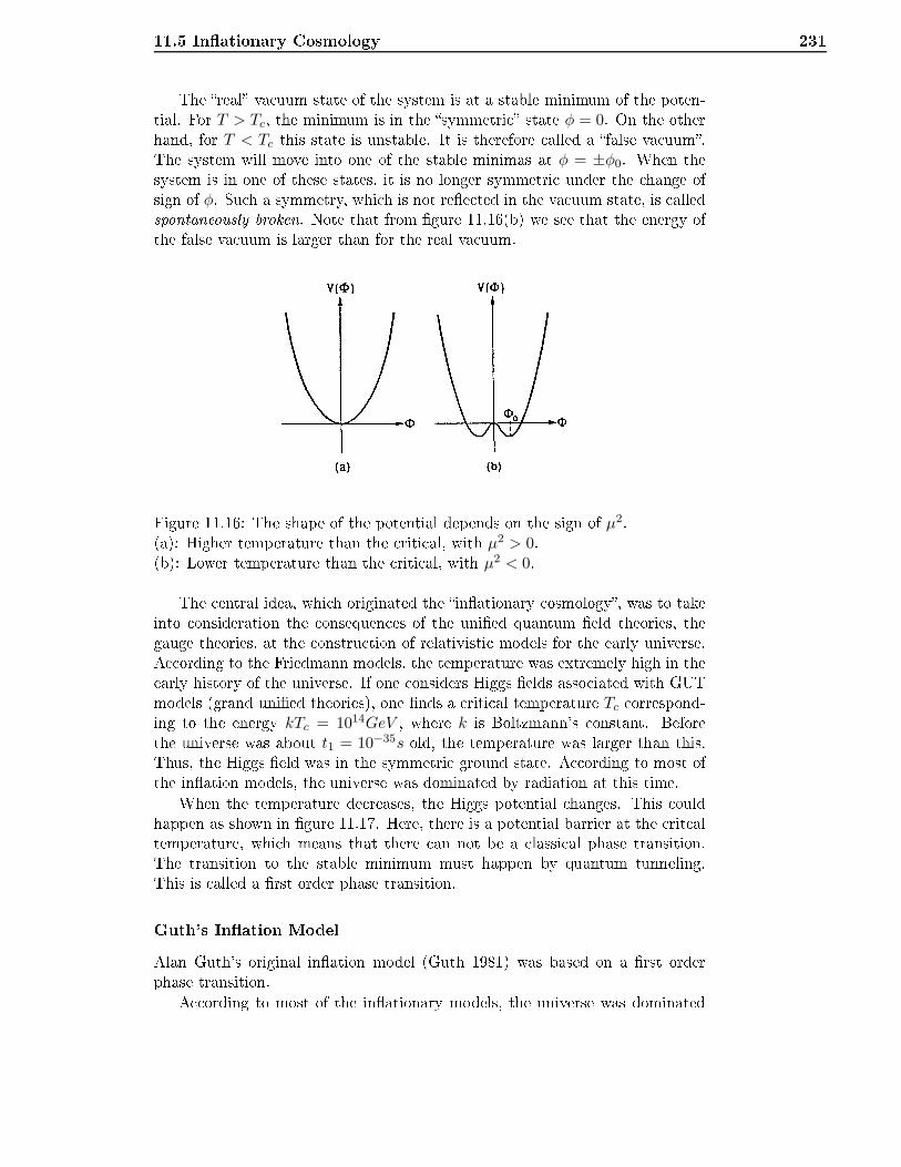
11.5 Inationary Cosmology 231The real va uum state of the system is at a stable minimum of the poten-tial. For T > Tc, the minimum is in the symmetri state φ = 0. On the otherhand, for T < Tc this state is unstable. It is therefore alled a false va uum.The system will move into one of the stable minimas at φ = ±φ0. When thesystem is in one of these states, it is no longer symmetri under the hange ofsign of φ. Su h a symmetry, whi h is not ree ted in the va uum state, is alledspontaneously broken. Note that from gure 11.16(b) we see that the energy ofthe false va uum is larger than for the real va uum.

Figure 11.16: The shape of the potential depends on the sign of µ2.(a): Higher temperature than the riti al, with µ2 > 0.(b): Lower temperature than the riti al, with µ2 < 0.The entral idea, whi h originated the inationary osmology, was to takeinto onsideration the onsequen es of the unied quantum eld theories, thegauge theories, at the onstru tion of relativisti models for the early universe.A ording to the Friedmann models, the temperature was extremely high in theearly history of the universe. If one onsiders Higgs elds asso iated with GUTmodels (grand unied theories), one nds a riti al temperature Tc orrespond-ing to the energy kTc = 1014GeV , where k is Boltzmann's onstant. Beforethe universe was about t1 = 10−35s old, the temperature was larger than this.Thus, the Higgs eld was in the symmetri ground state. A ording to most ofthe ination models, the universe was dominated by radiation at this time.When the temperature de reases, the Higgs potential hanges. This ouldhappen as shown in gure 11.17. Here, there is a potential barrier at the rit altemperature, whi h means that there an not be a lassi al phase transition.The transition to the stable minimum must happen by quantum tunneling.This is alled a rst order phase transition.Guth's Ination ModelAlan Guth's original ination model (Guth 1981) was based on a rst orderphase transition.A ording to most of the inationary models, the universe was dominated

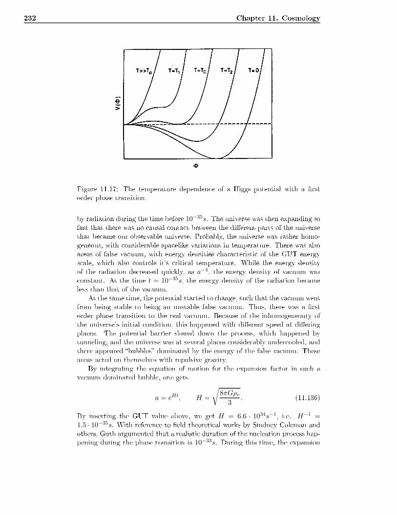
232 Chapter 11. Cosmology

Figure 11.17: The temperature dependen e of a Higgs potential with a rstorder phase transition.by radiation during the time before 10−35s. The universe was then expanding sofast that there was no ausal onta t between the dierent parts of the universethat be ame our observable universe. Probably, the universe was rather homo-geneous, with onsiderable spa elike variations in temperature. There was alsoareas of false va uum, with energy densities hara teristi of the GUT energys ale, whi h also ontrols it's riti al temperature. While the energy densityof the radiation de reased qui kly, as a−4, the energy density of va uum was onstant. At the time t = 10−35s, the energy density of the radiation be ameless than that of the va uum.At the same time, the potential started to hange, su h that the va uum wentfrom being stable to being an unstable false va uum. Thus, there was a rstorder phase transition to the real va uum. Be ause of the inhomogeneouty ofthe universe's initial ondition, this happened with dierent speed at dieringpla es. The potential barrier slowed down the pro ess, whi h happened bytunneling, and the universe was at several pla es onsiderably under ooled, andthere appeared bubbles dominated by the energy of the false va uum. Theseareas a ted on themselves with repulsive gravity.By integrating the equation of motion for the expansion fa tor in su h ava uum dominated bubble, one getsa = eHt, H =

√8πGρc

3. (11.136)By inserting the GUT value above, we get H = 6.6 · 1034s−1, i.e. H−1 =

1.5 · 10−35s. With referen e to eld theoreti al works by Sindney Coleman andothers, Guth argumented that a realisti duration of the nu leation pro ess hap-pening during the phase transition is 10−33s. During this time, the expansion

11.5 Inationary Cosmology 233fa tor in reases by a fa tor of 1028. This va uum dominated epo h is alled theination era.Let us look loser at what happens with the energy of the universe in the ourse of it's development, a ording to the inationary models. To understandthis we rst have to onsider what happens at the end of the inationary era.When the Higgs eld rea hes the minimum orresponding to the real va uum,it starts to os illate. A ording to the quantum des ription of the os illatingeld, the energy of the false va uum is onverted into radiation and parti les. Inthis way the equation of state for the energy dominating the development of theexpansion fa tor hanges from p = −ρ, hara teristi for va uum, to p = 13ρ, hara teristi of radiation.The energy density and the temperature of the radiation is then in reasedenourmously. Before and after this short period around the time t = 10−33s theradiation energy in reases adiabati ally, su h that ρa4 = onstant. A ording toStefan-Boltzmanns law of radiadion, ρ ∝ T 4. Therefore, aT = onstant duringadiabati expansion. This means that during the inationary era, while theexpansion fa tor in reases exponentially, the energy density and temperatureof radiation de reases exponentially. At the end of the inationary era, theradiation is reheated so that it returns to the energy it had when the inationaryera started.It may be interesting to note that the Newtonian theory of gravitation doesnot allow an inationary era, sin e stress has no gravitational ee t a ordingto it.The Ination Models' Answers to the Problems of the FriedmannModelsThe horizon problem will here be investigated in the light of this model. Theproblem was that there was room for about 10000 ausally onne ted areasinside the area spanned by our presently observable universe at the time. Let us al ulate the horizon radius lh and the radius a of the region presently withinthe horizon, lh = 15 · 109ly = 1.5 · 1026cm, at the time t1 = 10−35s when theination started. From equation (11.128) for the radiation dominated periodbefore the inatinary era, one gets

lh = 2t1 = 6 · 10−25cm. (11.137)The radius, at time t1, of the region orresponding to our observable universe,is found by using that a ∝ eHt during the ination era from t1 = 10−35s tot2 = 10−33s, a ∝ t

12 in the radiation dominated period from t2 to t3 = 1011s,and a ∝ t

23 in the matter dominated period from t3 until now, t0 = 1017s. Thisgivesa1 =

eHt1

eHt2

(t2t3

) 12(t3t0

) 23

lh(t0) = 1.5 · 10−28cm. (11.138)We see that at the beginning of the inationary era the horizon radius,lh, was larger than the radius a of the region orresponding to our observable

234 Chapter 11. Cosmologyuniverse. The whole of this region was then ausally onne ted, and thermi equilibrium was established. This equilibrium has been kept sin e then, andexplains the observed isotropy of the osmi ba kground radiation.We will now onsider the atness problem. This problem was the ne essity,in the Friedmann models, of ne tuning the initial density in order to obtainthe loseness of the observed mass density to the riti al density. Again, theinationary models give another result. Inserting the expansion fa tor (11.136)into equation (11.132), we getΩ − 1 =

k

H2e−2Ht, (11.139)where H is onstant and given in eq. (11.136). The ratio between Ω − 1 at theend of and the beginning of the inationary era be omes

Ω2 − 1

Ω1 − 1= e−2H(t2−t1) = 10−56. (11.140)Contrary to in the Friedmann models, where the mass density moves awayfrom the riti al density as time is in reasing, the density approa hes the riti aldensity exponentially during the inationary era. Within a large range of initial onditions, this means that a ording to the ination models the universe shouldstill have almost riti al mass density.

Problems 235Problems11.1. Cosmi redshiftWe shall in this problem study the osmi redshift in an expanding FRW uni-verse and show that this redshift, for small distan es between emitter and re- eiver, an be split into a gravitational and a kinemati part.(a) Show that the assumption that the distan e between emitter and re eiveris small, an be expressed asH0(t0 − te) ≪ 1.Here, the lower index of 0 and emean evaluated at the re eiver and emitter,respe tively.In the following, in lude only terms to 2nd order in H0(t0 − te).(b) Light is emitted at wavelength λe and re eived at λ0. Show that theredshift, z, an be written as

z = H0(t0 − te) +(1 +

q02

)H2

0 (t0 − te)2, (11.141)where q is the de eleration parameter. We introdu e zK and zG, the kine-mati and the gravitational redshift, dened as follows. zK is the redshiftof light emitted due to the velo ity with respe t to the observer, of theemitter. zG is the redshift of light for an emitter who has a xed distan eto the re eiver. Show that z ≈ zK + zG for zK ≪ 1 og zG ≪ 1. Use theDoppler shift formula from the spe ial theory of relativity

zK = [(1 + Ve)/(1 − Ve)]1/2 − 1. (11.142)to nd zK . Show further that

zG = −1

2q0H

20 (t0 − te)

2. (11.143)Why has zG the sign it has?The universe is matter dominated at t0, nad thus p ≪ ρ, where p is thepressure and ρ is the energy-density of the osmi uid. Show that, usingthe Friedmann equations,q0H

20 =

4π

3Gρ0, ρ0 = ρ(t0). (11.144)Dene the osmi gravitational potential, φe, in the Newtonian approxi-mation su h that φe = 0 at the position of the re eiver. Show lastly thatzG = −φe. (11.145)11.2. Gravitational ollapseIn this problem we shall nd a solution to Einstein's eld equations des ribinga spheri al symmetri gravitational ollapse. The solution shall des ribe the

236 Chapter 11. Cosmologyspa etime both exterior and interior to the star. To onne t the exterior andinterior solutions, the metri s must be expressed in the same oordinate system.We will assume that the interior solution has the same form as a Friedmannsolution. The Friedmann solutions are expressed in omoving oordinates, thusfreely falling parti les have onstant spatial oordinates.Let (ρ, τ) be the infalling oordinates. τ is the proper time to a freely fallingparti le starting at innity with zero velo ity. These oordinates are onne tedto the S hwarzs hild oordinates via the requirementsρ = r, for τ = 0

τ = t, for r = 0. (11.146)(a) Show that the transformation between the infalling oordinates and theS hwarzs hild oordinates is given byτ =

2

3(2M)−

12

(ρ

32 − r

32

),

t = τ − 4M( r

2M

) 12

+ 2M ln

(r

2M

) 12 + 1

(r

2M

) 12 − 1

,whereM is the S hwarzs hild mass of the star. Show that the S hwarzs hildmetri in these oordinates takes the formds2 = −dτ2 +

[1 − 3

2(2M)

12 τρ−

32

]− 23

dρ2

+

[1 − 3

2(2M)

12 τρ−

32

] 43

ρ2(dθ2 + sin2 θdφ2

). (11.147)Show that the metri is not singular at the S hwarzs hild radius. Whereis it singular?(b) Assume the star has a position dependent energy-density (τ), and thatthe pressure is zero. Assume further that the interior spa etime an bedes ribed with a Friedmann solution with Eu lidean geometry (k = 0).Find the solution when the radius of the star is R0 at τ = 0.11.3. Physi al signi an e of the Robertson-Walker oordinate systemShow that the referen e parti les with xed spatial oordinates move alonggeodesi world lines, and hen e are free parti les.11.4. The volume of a losed Robertson-Walker universeShow that the volume of the region ontained inside a radius r = aχ = a arcsin ris

V = 2πa3

(χ− 1

2sin 2χ

).Find the maximal volume. Find also an approximate expression for V when

χ≪ R.

Problems 23711.5. The past light- one in expanding universe models(a) Show that the radial standard oordinate of the past light- one isχl (te) = c

∫ t0

te

dt

a(t). (11.148)(b) The proper distan e at a point of time t to a parti le at a radial oordinate

χ is d = a(t)χ. Dierentiation gives d = aχ+ aχ whi h may be writtenvtot = vre + vpe , (11.149)where vtot is the total radial velo ity of the parti le; vre is its re essionvelo ity ; and vpe is its pe uliar velo ity .Show that the re ession velo ity of a light sour e with redshift z is givenby

vre (z) = cE(z)

1 + z

∫ z

0

dy

E(y). (11.150)Can this velo ity be greater than the speed of light? What is the totalvelo ity of a photon emitted towards χ = 0? Is it possible to observe agalaxy with re ession velo ity greater than the speed of light?( ) Make a plot of the past light- one; i.e. of te as a fun tion of the properdistan e

dl = a(te)χl (te),for a at, matter dominated universe model. Explain the shape of thelight- one using that its slope is equal to the total velo ity of a photonemitted towards an observer at the origin.(d) Introdu e onformal time and al ulate the oordinate distan e of the pastlight- one as a fun tion of onformal time for the at, matter dominateduniverse model. Make a plot of the past light- one in these variables.11.6. Lookba k timeThe lookba k time of an obje t is the time required for light to travel from anemitting obje t to the re eiver. Hen e, it is tL ≡ t0 − te, where t0 is the pointof time that the obje t is observed and te is the point of time the light wasemitted.(a) Show that the lookba k time is given bytL =

1

H0

∫ z

0

dy

(1 + y)E(y), (11.151)where z is the redshift of the obje t.(b) Show that tL = t0

[1 − (1 + z)−3/2

], where t0 = 2/(3H0), in a at, matter-dominated universe.

238 Chapter 11. Cosmology( ) Show that the lookba k time in the Milne universe model with a(t) =(t/t0), k < 0, is

tL =1

H0

z

1 + z.(d) Make a plot with tL as a fun tion of z for the last two universe models.11.7. The FRW-models with a w-law perfe t uidIn this problem we will investigate FRW models with a perfe t uid. We willassume that the perfe t uid obeys the equation of state

p = wρ (11.152)where −1 ≤ w ≤ 1.(a) Write down the Friedmann equations for a FRWmodel with a w-law perfe tuid. Express them in terms of the s ale fa tor a only.(b) Assume that a(0) = 0. Show that when −1/3 < w ≤ 1, the losed modelwill re ollapse. Explain why this does not happen in the at and openmodels.( ) Solve the Friedmann equation for a general w 6= −1 in the at ase. Whatis the Hubble parameter and the de eleration parameter? Write also downthe time evolution for the matter density.(d) Find the parti le horizon distan e in terms of H0, w and z.(e) Spe ialize the above to the dust and radiation dominated universe models.11.8. Age-density relations(a) Show that the age of a radiation dominated universe model is given byt0 =

1

H0· 1

1 +√

Ωγ0

, (11.153)for all values of k.(b) Show that the age of a matter dominated universe model with k > 0 maybe expressed byt0 =

Ωm0

2H0(Ωm0 − 1)32

[arccos

(2

Ωm0− 1

)− 2

Ωm0(Ωm0 − 1)

12

] (11.154)and of a matter dominated universe model with k < 0

t0 =Ωm0

2H0(1 − Ωm0)32

[2

Ωm0(1 − Ωm0)

12 − arccosh

(2

Ωm0− 1

)].(11.155)( ) Show that the lifetime of the losed universe is

T =π

H0

Ωm0

(Ωm0 − 1)32

, (11.156)

Problems 239and that the s ale fa tor at maximum expansion isamax =

Ωm0

Ωm0 − 1. (11.157)11.9. Redshift-luminosity relation for matter dominated universeShow that the luminosity distan e of an obje t with redshift z in a matterdominated universe with relative density Ω0 and Hubble parameter H0 is

dL =2c

H0Ω20

[Ω0z + (Ω0 − 2)(

√1 + Ω0z − 1)

]. (11.158)For the Einstein-de Sitter universe, with Ω0 = 1, this relation redu es to

dL =2c

H0(1 + z −

√1 + z). (11.159)Plot this distan e in light years as a fun tion of z for a universe with Hubbleparameter H0 = 20km/s per light years.11.10. Newtonian approximation with va uum energyShow that Einstein's linearised eld equations for a stati spa etime ontainingdust with density ρ and va uum energy with density ρΛ takes the form of amodied Poisson equation

∇2φ = 4πG(ρ − 2ρΛ). (11.160)11.11. Universe models with onstant de eleration parameter(a) Show that the universe with onstant de eleration parameter q has expan-sion fa tora =

(t

t0

) 11+q

, q 6= −1, and a ∝ eHt, q = −1.(b) Find the Hubble length ℓH = H−1 and the radius of the parti le horizonas fun tions of time for these models.11.12. Relative densities as fun tions of the expansion fa torShow that the relative densities of matter and va uum energy as fun tions of aareΩv =

Ωv0a3

Ωv0a3 + (1 − Ωv0 − Ωm0) a+ Ωm0

Ωm =Ωm0

Ωv0a3 + (1 − Ωv0 − Ωm0) a+ Ωm0(11.161)What an you on lude from these expressions on erning the universe at earlyand late times?

240 Chapter 11. Cosmology11.13. FRW universe with radiation and matterShow that the expansion fa tor and the osmi time as fun tions of onformaltime of a universe with radiation and matter arek > 0 :

a = a0 [α(1 − cos η) + β sin η]

t = a0 [α(η − sin η) + β(1 − cos η)](11.162)

k = 0 :

a = a0

[12αη

2 + βη]

t = a0

[16αη

3 + 12βη

2] (11.163)

k < 0 :

a = a0 [α(cosh η − 1) + β sinh η]

t = a0 [α(sinh η − η) + β(cosh η − 1)](11.164)where α = a2

0H20Ωm0/2 and β = (a2

0H20Ωγ0)

1/2, and Ωγ0 and Ωm0 are the presentrelative densities of radiation and matter, H0 is the present value of the Hubbleparameter.11.14. Matter-va uum transition in the Friedmann-Lemaître modelFind the point of time of transition from matter domination to va uum dom-ination of the at Friedmann-Lemaître universe model and the orrespondingredshift.11.15. Event horizons in de Sitter universe modelsShow that the oordinate distan es to the event horizons of the de Sitter universemodels with k > 0, k = 0 and k < 0 are (assuming Λ = 3)rEH = 1

cosh t , k > 0, t ≥ 0rEH = e−t, k = 0,rEH = 1

sinh t , k < 0, t ≥ 0respe tively.11.16. Light travel timeIn this problem you are going to al ulate the light travel time of light from anobje t with redshift z in a at Friedmann-Lemaître model with age t0 and apresent relative density of LIVE, ΩΛ0.Show that the point of time of the emission event iste = t0

arcsinh√

ΩΛ0(1−ΩΛ0)(1+z)3

arcsinh√

ΩΛ01−ΩΛ0

, (11.165)and al ulate the light travel time t0 − te. Make a plot of (t0 − te)/t0 as afun tion of z.11.17. Superluminal expansionShow from Hubble's law that all all obje ts in a at Friedmann-Lemaître model

Problems 241with redshifts z > zc are presently re eding faster than the speed of light, wherezc is given by ∫ 1+zc

0

dy√ΩΛ0 + Ωm0y3

= 1. (11.166)Find zc for a universe model with ΩΛ0 = 0.7 and Ωm0 = 0.3.11.18. Flat universe model with radiation and va uum energy(a) Find the expansion fa tor as a fun tion of time for a at universe with radi-ation and Lorentz-invariant va uum energy represented by a osmologi al onstant Λ, and with present relative density of va uum energy Ωv0.(b) Cal ulate the Hubble parameter, H, as a fun tion of time, and show thatthe model approa hes a de Sitter model in the far future. Find also thede eleration parameter, q(t).( ) When is the ine tion point, t1, for whi h the universe went from de eler-ation to a eleration? What is the orresponding redshift observed at thetime t0?11.19. Creation of radiation and ultra-relativisti gas at the end of the ination-ary eraAssume that the va uum energy an be des ribed by a de aying osmologi alparameter Λ(t). Show from energy onservation that if the density of radiationand gas is negligible at the nal period of the inationary era ompared to afterit, then the density immediately after the inationary era isρ =

1

8πGa(t)4

∫ t2

t1

Λa(t)4dt (11.167)where t2 − t1 is the duration of the period with Λ 6= 0.11.20. Phantom EnergyConsider a at universe model dominated by quintessen e energy with equationof state, p = wρ, w = constant. We shall onsider 'phantom energy' withw < −1(a) Use the normalization a(t0) = 1 and nd the s ale fa tor a as a fun tionof osmi time.(b) Find the energy density as a fun tion of time.( ) Show that the s ale fa tor and the density blows up to innity at a time

tr = t0 −2

3(1 + w)H0

√ΩP0

, (11.168)where ΩP0 is the relative density of the phantom energy at the presenttime. The osmi atastrophe at the time tr is alled 'the Big Rip'. Whatis tr − t0 for H0 = 20km/s per 106ly, ΩP0 = 0.64, and w = −3/2?

242 Chapter 11. Cosmology(d) A planet in an orbit of radius R around a star of mass M will be omeunbound roughly when −(4π/3)(ρ + 3p)R3 ≈ M , where ρ and p are thedensity and the pressure of the phantom energy.Show that a gravitationally bound system of mass M and radius R will bestripped at a time ts before the big rip, given byts ≈ −

√−2(1 + 3w)

6π(1 + w)T,where T is the period of a ir ular orbit with radius R around the system.Find ts for the Milky Way galaxy with w = −3/2.

BibliographyBernadis et.al, P. d.: 2001, Multiple peaks in the angular power spe trum ofthe osmi mi rowave ba kground: Signi an e and onsequen es for os-mology, astro-ph/0105296.Brill, D. R. and Cohen, J. M.: 1966, Phys. Rev. 143, 1011.Carroll, S. M.: 1998, Quintessen e and the rest of the world., Phys. Rev. Lett.81, 30673070.Carroll, S. M.: 2001, Dark energy and the preposterous universe., astro-ph/0107571.Grøn, Ø.: 1986, Repulsive gravitation and inationary universe models., 54, 4652.Grøn, Ø. and Flø, H. K.: 1984, Dierensialgeometri, Departmental. Course ompendium.Guth, A. H.: 1981, The inationary universe: a possible solution to the horizonand atness problems, Phys. Rev. D23, 347356.Linde, A.: 2001, Ination and string osmology, astro-ph/0107176.M Gaugh, S.: 2001, Constraints on the radial mass distribution of dark matterhalos from rotation urves, astro.ph/0107490.Misner, C. W., Thorne, K. S. and Wheeler, J. A.: 1973, Gravitation, rst edn,W. H. Freeman and ompany, San Fran is o.Perlmutter et al., S.: 1999, Measurements of omega ans lambda from 42 high-redshift supernovae., Astrophys. J. 517, 565586.Pound, R. V. and Rebka, G. A., J.: 1960, Phys. Review Letters 4, 337.Pryke et al., C.: 2001, Cosmologi al parameter extra tion from the rst seasonof observations with dasi., astro-ph/0104490.Ravndal, F.: 1978, Inføring i generell relativitetsteori, Departmental. Course ompendium.Riess, A. G.: n.d., The farthest known supernova: Support for an a eleratinguniverse and a glimpse of the epo h of de eleration., astro-ph/0104455.243

244 BIBLIOGRAPHYRiess et al., A. G.: 1998, Observational eviden e from supernovae for an a el-erating universe and a osmologi al onstant., Astron. J. 116, 10091038.Stompor et al., R.: 2001, Cosmologi al impli ations of the maxima-i highresolution osmi mi rowave ba kground anisotropy measurement., astro-ph/0105062.Turner, M. S.: 2001, Dark energy and the new osmology., astro-ph/0108103.Turner, M. S. and Riess, A. G.: 2001, Do Sn Ia provide dire t eviden e for pastde eleration of the universe?, astro-ph/0106051.Zeldovi h, Y.: 1968, The osmologi al onstant and the theory of elementaryparti les, Sov. Phys. Usp. 11, 381393.Zlatev, I., Wang, L. and Steinhardt, P. J.: 1999, Quintessen e, osmi oin i-den e, and the osmologi al onstant, Phys. Rev. Lett. 82, 896899.

IndexSymbols, ν1ν2 . . . . . . . . . . . . . . . . . . . . . . . . . . . . . . 50δS = 0 . . . . . . . . . . . . . . . . . . . . . . . . . . . . .58δ(~r) (Dira delta fun tion) . . . . . . . . . . 4γij . . . . . . . . . . . . . . . . . . . . . . . . . . . . . . . . . 34⊗ (tensor produ t). . . . . . . . . . . . . . . . .26d2α . . . . . . . . . . . . . . . . . . . . . . . . . . . . . . . . 51dΩ (solid angle) . . . . . . . . . . . . . . . . . . . . . 5dt . . . . . . . . . . . . . . . . . . . . . . . . . . . . . . . . . 35dl2 . . . . . . . . . . . . . . . . . . . . . . . . . . . . . . . . 34[ (antisymmetri ombination) . . . . 32Γαµν . . . . . . . . . . . . . . . . . . . . . . . . . . . . . . . 603-spa e . . . . . . . . . . . . . . . . . . . . . . . . . . . . 344-a eleration . . . . . . . . . . . . . . . . . 16, 1214-momentum . . . . . . . . . . . . . . . . . . . . . . 154-velo ity . . . . . . . . . . . . . . . . . . . . . . . . . . 15identity . . . . . . . . . . . . . . . . . . . . 16, 58Aa elerated framehyperboli ally . . . . . . . . . . . . . . . . . 44a eleration of parti lein non-rotating frame . . . . . . . . . . 73in rotating frame . . . . . . . . . . . . . . 73a eleration s alar . . . . . . . . . . . . . . . . 121a tion . . . . . . . . . . . . . . . . . . . . . . . . . . . . . 57Ar himedean spiral . . . . . . . . . . . . . . . . 41Bbasis1-form. . . . . . . . . . . . . . . . . . . . . . . . . 25 oordinate basis ve tor . . . . . 18, 21orthonormal . . . . . . . . . . . . . . . 18, 22Bian hi1st identity . . . . . . . . . . . . . . . . 90, 92 omponent form . . . . . . . . . . . . . 912nd identity. . . . . . . . . . . . . . . .91, 95bla k holehorizon . . . . . . . . . . . . . . . . . . . . . . . 121

mini . . . . . . . . . . . . . . . . . . . . . . . . . . 123radiation . . . . . . . . . . . . . . . . . . . . . 122temperature . . . . . . . . . . . . . . . . . . 122Born-sti motion . . . . . . . . . . . . . . . . . . 44C anoni al momentum . . . . . . . . . . . . . . 58Cartanformalism . . . . . . . . . . . . . . . . . . . . 100stru ture equations1st . . . . . . . . . . . . . . . . . . . . . 79, 1002nd. . . . . . . . . . . . . . . . . . . . . 85, 101surfa e urvature . . . . . . . . . . . . . . 89 entrifugal a eleration . . . . . . . . . . . . 74 entrifulgal barrier . . . . . . . . . . . . . . . . 114Christoel symbols . . . . . . . . . . . . . . . . 60in oordinate basis . . . . . . . . . . . . .53physi al interpretation. . . . . . . . 103rotating referne e frame . . . . . . . 73 omoving orthonormal basis . . . . . . . 31 onne tion oe ientsin a Riemannian spa e . . . . . . . . . 74in oordinate basis . . . . . . . . . . . . .53rotating referen e frame . . . . . . . 72 onne tion forms . . . . . . . . . . . . . . . . . 100 onservationenergy-momentum . . . . . . . . . . . . . 93 onstant of motion . . . . . . . . . . . . . . . . . 58 ontinuity equation . . . . . . . . . . . . . . . . 93 ontravariant tensor . . . . . . . . . . . . . . . 26 onve tive derivative . . . . . . . . . . . . . . . 93 oordinate y li . . . . . . . . . . . . . . . . . . . . . . 58, 59Gaussian . . . . . . . . . . . . . . . . . . . . . . 54transformation . . . . . . . . . . . . . 20, 27 oordinate basis . . . . . . . . . . . . . . . . 18, 21 onne tion oe ients . . . . . . . . . 53 oordinate system . . . . . . . . . . . . . . . . . 18245

246 INDEX oriolis a eleration . . . . . . . . . . . . . . . . 74 osmologi al redshift . . . . . . . . . . . . . .136 ovarian e prin iple . . . . . . . . . . . . 11, 51 ovariant equations . . . . . . . . . . . . . . . . 28 ovariant tensor. . . . . . . . . . . . . . . . . . . .26 urvature . . . . . . . . . . . . . . . . . . . . . . . . . . 81forms . . . . . . . . . . . . . . . . . . . . . 85, 101of surfa e . . . . . . . . . . . . . . . . . . . . 89Gaussian. . . . . . . . . . . . . . . . . . .88, 89geodesi . . . . . . . . . . . . . . . . . . . . . . . 87normal . . . . . . . . . . . . . . . . . . . . . . . . 87prin ipal. . . . . . . . . . . . . . . . . . . . . . .88Ri i . . . . . . . . . . . . . . . . . . . . . . . . . . 91Riemann tensor. . . . . . . . . . . . . . . .83surfa e (Cartan formalism) . . . . 89Ddee tion of light . . . . . . . . . . . . . . . . . 119dierential forms1-form. . . . . . . . . . . . . . . . . . . . . . . . . 252-form. . . . . . . . . . . . . . . . . . . . . . . . . 32 omponents . . . . . . . . . . . . . . . . . . . 33 onne tion . . . . . . . . . . . . . . . . . . . 100 ovariant dierentiation of . . . . . 75 urvature . . . . . . . . . . . . . . . . . 85, 101of surfa e . . . . . . . . . . . . . . . . . . . . 89dierentiation of . . . . . . . . . . . . . . . 49dire tional derivatives of . . . . . . . 76null form . . . . . . . . . . . . . . . . . . . . . . 33p-form. . . . . . . . . . . . . . . . . . . . . . . . .32transformation. . . . . . . . . . . . . . . . .27dierentiation onve tive . . . . . . . . . . . . . . . . . . . . . 93 ovariant. . . . . . . . . . . . . . . . . . .53, 55exterior. . . . . . . . . . . . . . . . . . . . . . . .49of form . . . . . . . . . . . . . . . . . . . . . . . . 49Dira delta fun tion. . . . . . . . . . . . . . . . .4distan e oordinate . . . . . . . . . . . . . . . . . . . . 100physi al . . . . . . . . . . . . . . . . . . . . . . 100Doppler ee t . . . . . . . . . . . . . . . . . . . . . 23Doppler ee t, gravitational . . . . . . . 70dust dominated universe . . . . . . . . . . 143EEddington - Finkelstein oordinates104

Einsteineld equations . . . . . . . . . . . . . . . . . 96prin iple of equivalen e . . . . . . . . . 9syn hronization . . . . . . . . . . . . . . . . 35tensor . . . . . . . . . . . . . . . . . . . . . . . . . 96Einstein deSitter universe . . . . . . . . . 145embeddingof the S hwarzs hild metri . . . 110energy-momentum tensor . . . . . . . . . . 93equivalen e, prin iple of . . . . . . . . . . . . . 9Euler equation of motion . . . . . . . . . . 93Euler-Lagrange equations . . . . . . . . . . 58exterior dierentiation . . . . . . . . . . . . . 49Feld equationsEinstein . . . . . . . . . . . . . . . . . . . . . . . 96va uum. . . . . . . . . . . . . . . . . . . . . . . .97rst order phase transition . . . . . . . . 161atness problem . . . . . . . . . . . . . 159, 164forms . . . . . . . . . . . see dierential formsfree fall . . . . . . . . . . . . . . . . . . . . . . . . . . . 104GGauss oordinates . . . . . . . . . . . . . . . . . . . . 54 urvature . . . . . . . . . . . . . . . . . . 88, 89integral theorem . . . . . . . . . . . . . . . . 4theorema egregium . . . . . . . . . . . . 89general prin iple of relativity. . . . . . .10geodesi urvature . . . . . . . . . . . . . . . . . . . . . . 87 urve . . . . . . . . . . . . . . . . . . . . . . 57, 60spatial. . . . . . . . . . . . . . . . . . . . . . .62equation . . . . . . . . . . . . . . . . . . . . . . . 56postulate . . . . . . . . . . . . . . . . . . . . . . 98gravitational a eleration . . . . . . . . . 103Tolman-Whittaker expression . 129gravitational ollapse . . . . . . . . . . . . . 114gravitational time dilation . . . . . . . . . 40Grøn, Øyvind. . . . . . . . . . . . . . . . . . . . . . . 3Guth, Alan . . . . . . . . . . . . . . . . . . . . . . . 162HHafele-Keating experiment . . . . . . . . 116Hamilton-prin iple . . . . . . . . . . . . . . . . . 57Hawking radiation . . . . . . . . . . . . . . . . 122

INDEX 247heat apa ity of bla k hole . . . . . . . . 122Higgs me hanism . . . . . . . . . . . . . . . . . 160horizon problem . . . . . . . . . . . . . 157, 163Hubbles law . . . . . . . . . . . . . . . . . . . . . . 136hydrostati equilibrium . . . . . . . . . . . 128hyperboli ally a elerated frame . . . 44Iin ompressible stars . . . . . . . . . . . . . . 132inertial referen e frame . . . . . . . . . . . . 18inertial dragging . . . . . . . . . . . . . . . . . . 124inertial referen e frame . . . . . . . . . . . . 54ination . . . . . . . . . . . . . . . . . . . . . . . . . . 162KKerr metri . . . . . . . . . . . . . . . . . . . . . . . 123Krets hmann's urvature s alar . . . 104Kruskal - Szekers . . . . . . . . . . . . . . . . . 104Kruskal-Szekers . . . . . . . . . . . . . . . . . . . 108LLagrange ovariant dynami s . . . . . . . . . . . . 57equations . . . . . . . . . . . . . . . . . . . . . . 58free parti le . . . . . . . . . . . . . . . . . 60fun tion . . . . . . . . . . . . . . . . . . . . . . . 57free parti les . . . . . . . . . . . . . . . . 60Lapla e equation. . . . . . . . . . . . . . . . . . . . 3Levi-Civita onne tion . . . . . . . . . . . . . 53lightde eleration of . . . . . . . . . . . . . . . . 110dee tion of . . . . . . . . . . . . . . . . . . 119light ones . . . . . . . . . . . . . . . . . . . . . . . . 106line element . . . . . . . . . . . . . . . . . . . . . . . 31free parti le . . . . . . . . . . . . . . . . . . . 59in spa e . . . . . . . . . . . . . . . . . . . . . . . 34spa etime . . . . . . . . . . . . . . . . . . . . . 35Lorentz transformation . . . . . . . . . . . . 23MMa h's prin iple . . . . . . . . . . . . . . . . . . . 12metri ovariant dierentiation. . . . . . . .77Kerr (rotating) . . . . . . . . . . . . . . . 123stati ,stationary . . . . . . . . . . . . . . . 59tensor . . . . . . . . . . . . . . . . . . . . . . . . . 28mini bla k holes . . . . . . . . . . . . . . . . . . 123

Minkowski spa e-timefrom S hwarzs hild solution . . 103mixed tensor. . . . . . . . . . . . . . . . . . . . . . .26momentum-energy tensor . . . . . . . . . . 93NNewtonuid . . . . . . . . . . . . . . . . . . . . . . . . . . . 94hydrodynami s . . . . . . . . . . . . . . . . 93law of gravitation . . . . . . . . . . . . . . . 1 ontinuous distribution . . . . . . . 2lo al form . . . . . . . . . . . . . . . . . . . . 2Newtonian in ompressible star . . . . 127Oorbit equation . . . . . . . . . . . . . . . . . . . . 115orthonormal basis . . . . . . . . . . . . . . . . . .18Pparallel transport . . . . . . . . . . . . . . 55, 81parti le traje toryS hwarzs hild 3-spa e . . . . . . . . 112Poin aré's lemma . . . . . . . . . . . . . . . . . . 51pre essionof Mer ury's perihelion . . . . . . . 118pressure for es . . . . . . . . . . . . . . . . . . . . 128prin iple of equivalen e. . . . . . . . .9, 103proje tile motion . . . . . . . . . . . . . . . . . . 66proper distan e . . . . . . . . . . . . . . . . . . . 136Rradiation dominated universe . . . . . 142rank . . . . . . . . . . . . . . . . . . . . . . . . . . . . . . . 26rapidity. . . . . . . . . . . . . . . . . . . . . . . . . . . .45redshift osmologi al . . . . . . . . . . . . . . . . . . 136Kerr spa etime . . . . . . . . . . . . . . . 124referen e frame . . . . . . . . . . . . . . . . . . . . 17inertial . . . . . . . . . . . . . . . . . . . . 18, 54relativity, general prin iple of . . . . . . 10Ri i urvature . . . . . . . . . . . . . . . . . . . . . . 91tensor, divergen e . . . . . . . . . . . 96identity. . . . . . . . . . . . . . . . . . . . . . . .90 omponent form . . . . . . . . . . . . . 90Riemann urvature tensor . . . . . 83, 101 omponents . . . . . . . . . . . . . . . . . . . 84

248 INDEXrotating bla k hole. . . . . . . . . . . . . . . .123rotating referen e frame. . . . . . . . . . . .64 onne tion oe ients . . . . . . . . . 72SSagna ee t . . . . . . . . . . . . . . . . . . . . . . 42S hwarzs hild3-spa e . . . . . . . . . . . . . . . . . . . . . . . 112energy. . . . . . . . . . . . . . . . . . . . . .112momentum . . . . . . . . . . . . . . . . . 112light ones. . . . . . . . . . . . . . . . . . . .106metri . . . . . . . . . . . . . . . . . . . . . . . . 104embedding . . . . . . . . . . . . . . . . . 110radius . . . . . . . . . . . . . . . . . 2, 104, 121solutioninterior . . . . . . . . . . . . . . . . . . . . . 132outer . . . . . . . . . . . . . . . . . . . . . . . 100spa etime. . . . . . . . . . . . . . . .104, 121simultaneityon Einstein syn hronized lo ks35spa e, geometry of . . . . . . . . . . . . . 35singularity oordinate . . . . . . . . . . . . . . . . . . . . 104physi al . . . . . . . . . . . . . . . . . . . . . . 104solid angle . . . . . . . . . . . . . . . . . . . . . . . . . . 4spheri al geometry . . . . . . . . . . . . . . . . . 38spontaneous symmetry breaking . . 161stru ture oe ients . . . . . . . . . . . . . . . 23in a Riemannian spa e . . . . . . . . . 74in oordinate basis . . . . . . . . . . . . .25surfa e urvature . . . . . . . . . . . . . . . . . . 89surfa e gravity . . . . . . . . . . . . . . . . . . . . 121Ttangent plane . . . . . . . . . . . . . . . . . . . . . . 17tensor . . . . . . . . . . . . . . . . . . . . . . . . . . . . . 25antisymmetri . . . . . . . . . . . . . . . . . 31 onstru tion example . . . . . . . . . . 27 ontra tion of . . . . . . . . . . . . . . . . . 91 ontravariant . . . . . . . . . . . . . . . . . . 26 ovariant . . . . . . . . . . . . . . . . . . . . . . 26 ovariant dierentiation of . . . . . 77Einstein . . . . . . . . . . . . . . . . . . . . . . . 96metri . . . . . . . . . . . . . . . . . . . . . . . . . 28mixed. . . . . . . . . . . . . . . . . . . . . .26, 28momentum energy . . . . . . . . . . . . . 93

produ t . . . . . . . . . . . . . . . . . . . . . . . 26rank . . . . . . . . . . . . . . . . . . . . . . . . . . . 26Ri i urvature . . . . . . . . . . . . . . . . 91Riemann urvature . . . . . . . 83, 101transformation properties . . . . . . 27theorema egregium . . . . . . . . . . . . . . . . 89tidal for es. . . . . . . . . . . . . . . . . . . . . . . . . .5time dilation, gravitational . . . . . . . . . 40Tolman-Oppenheimer-Volkov eq. . .131Tolman-Whittaker expression . . . . . 129travelling time . . . . . . . . . . . . . . . . . . . . 105Twin paradox . . . . . . . . . . . . . . . . . . . . 68Uuniverse modeldust dominated. . . . . . . . . . . . . . .143inationary. . . . . . . . . . . . . . . . . . . 162radiation dominated . . . . . . . . . . 142Vva uum eld equations . . . . . . . . . . . . . 97ve torbasis . . . . . . . . . . . . . . . . . . . . . . . . . . 14 ovariant dierentiation of . . . . . 75dimension . . . . . . . . . . . . . . . . . . . . . 13linearly independent . . . . . . . . . . . 13ZZAMO . . . . . . . . . . . . . . . . . . . . . . . . . . . 124