TM-Based SOC Models Augmented by Auxiliary Data for Carbon ... · Auxiliary Data for Carbon Crediting Programs in Semi-Arid Environments Salahuddin M. Jaber and Mohammed I. Al-Qinna

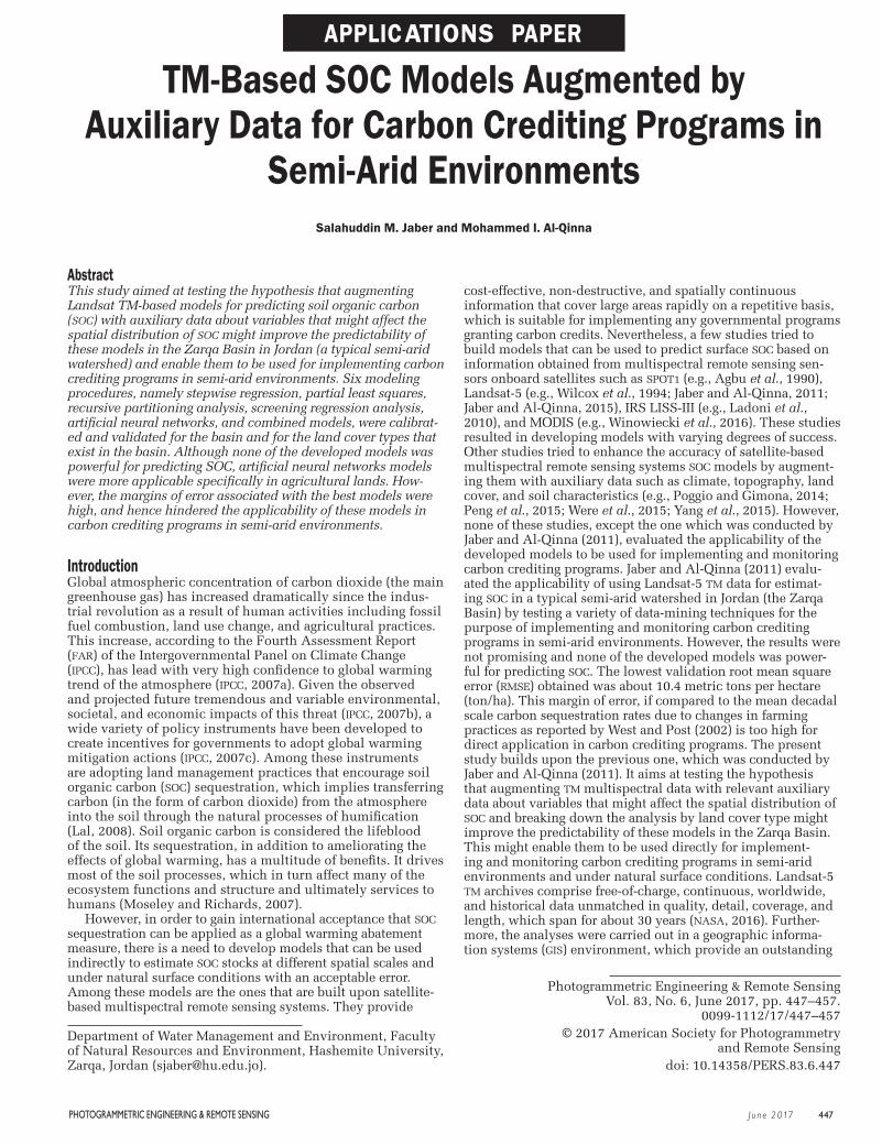
TM-Based SOC Models Augmented by Auxiliary Data for Carbon Crediting Programs in

Semi-Arid EnvironmentsSalahuddin M. Jaber and Mohammed I. Al-Qinna

Abstract This study aimed at testing the hypothesis that augmenting Landsat TM-based models for predicting soil organic carbon (SOC) with auxiliary data about variables that might affect the spatial distribution of SOC might improve the predictability of these models in the Zarqa Basin in Jordan (a typical semi-arid watershed) and enable them to be used for implementing carbon crediting programs in semi-arid environments. Six modeling procedures, namely stepwise regression, partial least squares, recursive partitioning analysis, screening regression analysis, artificial neural networks, and combined models, were calibrat-ed and validated for the basin and for the land cover types that exist in the basin. Although none of the developed models was powerful for predicting SOC, artificial neural networks models were more applicable specifically in agricultural lands. How-ever, the margins of error associated with the best models were high, and hence hindered the applicability of these models in carbon crediting programs in semi-arid environments.

IntroductionGlobal atmospheric concentration of carbon dioxide (the main greenhouse gas) has increased dramatically since the indus-trial revolution as a result of human activities including fossil fuel combustion, land use change, and agricultural practices. This increase, according to the Fourth Assessment Report (FAR) of the Intergovernmental Panel on Climate Change (IPCC), has lead with very high confidence to global warming trend of the atmosphere (IPCC, 2007a). Given the observed and projected future tremendous and variable environmental, societal, and economic impacts of this threat (IPCC, 2007b), a wide variety of policy instruments have been developed to create incentives for governments to adopt global warming mitigation actions (IPCC, 2007c). Among these instruments are adopting land management practices that encourage soil organic carbon (SOC) sequestration, which implies transferring carbon (in the form of carbon dioxide) from the atmosphere into the soil through the natural processes of humification (Lal, 2008). Soil organic carbon is considered the lifeblood of the soil. Its sequestration, in addition to ameliorating the effects of global warming, has a multitude of benefits. It drives most of the soil processes, which in turn affect many of the ecosystem functions and structure and ultimately services to humans (Moseley and Richards, 2007).

However, in order to gain international acceptance that SOC sequestration can be applied as a global warming abatement measure, there is a need to develop models that can be used indirectly to estimate SOC stocks at different spatial scales and under natural surface conditions with an acceptable error. Among these models are the ones that are built upon satellite-based multispectral remote sensing systems. They provide

cost-effective, non-destructive, and spatially continuous information that cover large areas rapidly on a repetitive basis, which is suitable for implementing any governmental programs granting carbon credits. Nevertheless, a few studies tried to build models that can be used to predict surface SOC based on information obtained from multispectral remote sensing sen-sors onboard satellites such as SPOT1 (e.g., Agbu et al., 1990), Landsat-5 (e.g., Wilcox et al., 1994; Jaber and Al-Qinna, 2011; Jaber and Al-Qinna, 2015), IRS LISS-III (e.g., Ladoni et al., 2010), and MODIS (e.g., Winowiecki et al., 2016). These studies resulted in developing models with varying degrees of success. Other studies tried to enhance the accuracy of satellite-based multispectral remote sensing systems SOC models by augment-ing them with auxiliary data such as climate, topography, land cover, and soil characteristics (e.g., Poggio and Gimona, 2014; Peng et al., 2015; Were et al., 2015; Yang et al., 2015). However, none of these studies, except the one which was conducted by Jaber and Al-Qinna (2011), evaluated the applicability of the developed models to be used for implementing and monitoring carbon crediting programs. Jaber and Al-Qinna (2011) evalu-ated the applicability of using Landsat-5 TM data for estimat-ing SOC in a typical semi-arid watershed in Jordan (the Zarqa Basin) by testing a variety of data-mining techniques for the purpose of implementing and monitoring carbon crediting programs in semi-arid environments. However, the results were not promising and none of the developed models was power-ful for predicting SOC. The lowest validation root mean square error (RMSE) obtained was about 10.4 metric tons per hectare (ton/ha). This margin of error, if compared to the mean decadal scale carbon sequestration rates due to changes in farming practices as reported by West and Post (2002) is too high for direct application in carbon crediting programs. The present study builds upon the previous one, which was conducted by Jaber and Al-Qinna (2011). It aims at testing the hypothesis that augmenting TM multispectral data with relevant auxiliary data about variables that might affect the spatial distribution of SOC and breaking down the analysis by land cover type might improve the predictability of these models in the Zarqa Basin. This might enable them to be used directly for implement-ing and monitoring carbon crediting programs in semi-arid environments and under natural surface conditions. Landsat-5 TM archives comprise free-of-charge, continuous, worldwide, and historical data unmatched in quality, detail, coverage, and length, which span for about 30 years (NASA, 2016). Further-more, the analyses were carried out in a geographic informa-tion systems (GIS) environment, which provide an outstanding

Department of Water Management and Environment, Faculty of Natural Resources and Environment, Hashemite University, Zarqa, Jordan ([email protected]).

Photogrammetric Engineering & Remote SensingVol. 83, No. 6, June 2017, pp. 447–457.

0099-1112/17/447–457© 2017 American Society for Photogrammetry

and Remote Sensingdoi: 10.14358/PERS.83.6.447

PHOTOGRAMMETRIC ENGINEERING & REMOTE SENSING J une 2017 447

06-17 June Peer Reviewed Digital.indd 447 5/17/2017 3:10:06 PM

frame for capturing, storing, querying, analyzing, and display-ing spatial data and information (Bolstad, 2012).

Materials and MethodsOverall Approach and Study AreaThe overall approach to this study consisted of: (a) compiling the auxiliary data needed to augment TM data in order to build models that can be used to predict surface SOC, (b) conducting data mining using TM and auxiliary data in order to develop the SOC models, (c) repeating and breaking down the data mining by land cover type in order to account for SOC vari-ability at different land cover types and test the effect of land cover on the modeling results, and (d) comparing the devel-oped models and evaluating the applicability of the best ones to be used directly for applying carbon crediting programs.

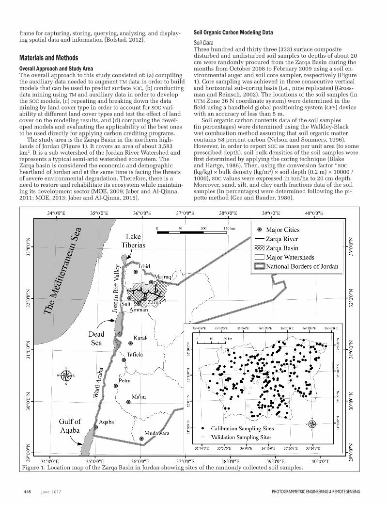
The study area is the Zarqa Basin in the northern high-lands of Jordan (Figure 1). It covers an area of about 3,583 km2. It is a sub-watershed of the Jordan River Watershed and represents a typical semi-arid watershed ecosystem. The Zarqa basin is considered the economic and demographic heartland of Jordan and at the same time is facing the threats of severe environmental degradation. Therefore, there is a need to restore and rehabilitate its ecosystem while maintain-ing its development sector (MOE, 2009; Jaber and Al-Qinna, 2011; MOE, 2013; Jaber and Al-Qinna, 2015).

Soil Organic Carbon Modeling Data

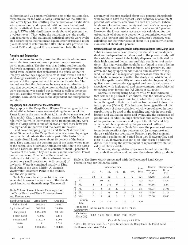
Soil DataThree hundred and thirty three (333) surface composite disturbed and undisturbed soil samples to depths of about 20 cm were randomly procured from the Zarqa Basin during the months from October 2008 to February 2009 using a soil en-vironmental auger and soil core sampler, respectively (Figure 1). Core sampling was achieved in three consecutive vertical and horizontal sub-coring basis (i.e., nine replicates) (Gross-man and Reinsch, 2002). The locations of the soil samples (in UTM Zone 36 N coordinate system) were determined in the field using a handheld global positioning system (GPS) device with an accuracy of less than 5 m.

Soil organic carbon contents data of the soil samples (in percentages) were determined using the Walkley-Black wet combustion method assuming that soil organic matter contains 58 percent carbon (Nelson and Sommers, 1996). However, in order to report SOC as mass per unit area (to some prescribed depth), soil bulk densities of the soil samples were first determined by applying the coring technique (Blake and Hartge, 1986). Then, using the conversion factor “SOC (kg/kg) × bulk density (kg/m3) × soil depth (0.2 m) × 10000 / 1000), SOC values were expressed in ton/ha to 20 cm depth. Moreover, sand, silt, and clay earth fractions data of the soil samples (in percentages) were determined following the pi-pette method (Gee and Bauder, 1986).

Figure 1. Location map of the Zarqa Basin in Jordan showing sites of the randomly collected soil samples.

448 J une 2017 PHOTOGRAMMETRIC ENGINEERING & REMOTE SENSING

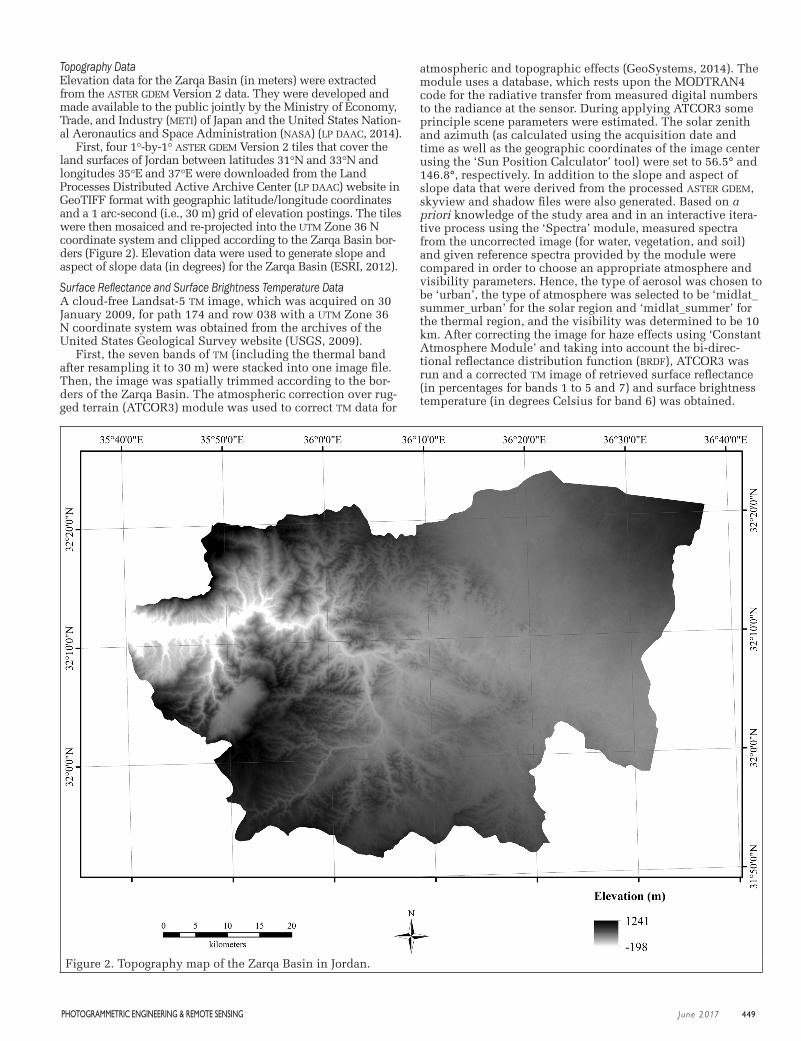
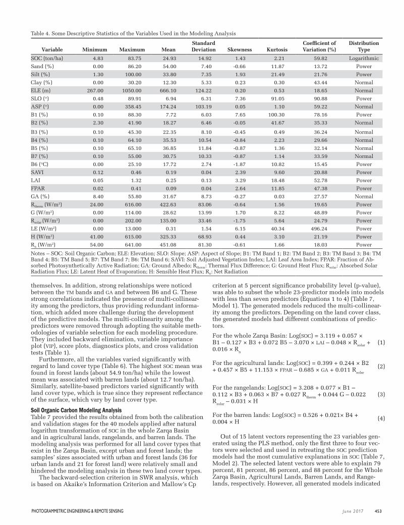
Topography DataElevation data for the Zarqa Basin (in meters) were extracted from the ASTER GDEM Version 2 data. They were developed and made available to the public jointly by the Ministry of Economy, Trade, and Industry (METI) of Japan and the United States Nation-al Aeronautics and Space Administration (NASA) (LP DAAC, 2014).

First, four 1°-by-1° ASTER GDEM Version 2 tiles that cover the land surfaces of Jordan between latitudes 31°N and 33°N and longitudes 35°E and 37°E were downloaded from the Land Processes Distributed Active Archive Center (LP DAAC) website in GeoTIFF format with geographic latitude/longitude coordinates and a 1 arc-second (i.e., 30 m) grid of elevation postings. The tiles were then mosaiced and re-projected into the UTM Zone 36 N coordinate system and clipped according to the Zarqa Basin bor-ders (Figure 2). Elevation data were used to generate slope and aspect of slope data (in degrees) for the Zarqa Basin (ESRI, 2012).

Surface Reflectance and Surface Brightness Temperature DataA cloud-free Landsat-5 TM image, which was acquired on 30 January 2009, for path 174 and row 038 with a UTM Zone 36 N coordinate system was obtained from the archives of the United States Geological Survey website (USGS, 2009).

First, the seven bands of TM (including the thermal band after resampling it to 30 m) were stacked into one image file. Then, the image was spatially trimmed according to the bor-ders of the Zarqa Basin. The atmospheric correction over rug-ged terrain (ATCOR3) module was used to correct TM data for

atmospheric and topographic effects (GeoSystems, 2014). The module uses a database, which rests upon the MODTRAN4 code for the radiative transfer from measured digital numbers to the radiance at the sensor. During applying ATCOR3 some principle scene parameters were estimated. The solar zenith and azimuth (as calculated using the acquisition date and time as well as the geographic coordinates of the image center using the ‘Sun Position Calculator’ tool) were set to 56.5° and 146.8°, respectively. In addition to the slope and aspect of slope data that were derived from the processed ASTER GDEM, skyview and shadow files were also generated. Based on a priori knowledge of the study area and in an interactive itera-tive process using the ‘Spectra’ module, measured spectra from the uncorrected image (for water, vegetation, and soil) and given reference spectra provided by the module were compared in order to choose an appropriate atmosphere and visibility parameters. Hence, the type of aerosol was chosen to be ‘urban’, the type of atmosphere was selected to be ‘midlat_summer_urban’ for the solar region and ‘midlat_summer’ for the thermal region, and the visibility was determined to be 10 km. After correcting the image for haze effects using ‘Constant Atmosphere Module’ and taking into account the bi-direc-tional reflectance distribution function (BRDF), ATCOR3 was run and a corrected TM image of retrieved surface reflectance (in percentages for bands 1 to 5 and 7) and surface brightness temperature (in degrees Celsius for band 6) was obtained.

Figure 2. Topography map of the Zarqa Basin in Jordan.


Value-Adding DataSubsequent to the atmospheric and topographic correction of TM image, two groups of value-adding products were calculated by ATCOR3 based on surface reflectance and temperature data. The first group includes: (1) soil adjusted vegetation index (SAVI), (2) leaf area index (LAI), (3) fraction of absorbed pho-tosynthetically active radiation (FPAR), and (4) ground albedo (GA). The second group includes: (1) absorbed solar radiation flux (Rsolar), (2) thermal flux difference (Rtherm), (3) ground heat flux (G), (4) latent heat of evaporation (LE), (5) sensible heat flux (H), and (6) net radiation (Rn). For details about the methodolo-gy used by ATCOR3 to calculate these ten variables, please refer to the ATCOR for IMAGINE 2015 user manual (GeoSystems, 2014) and ATCOR user guide (Richter and Schlapfer, 2014).

The first three variables (i.e., SAVI, LAI, and FPAR) are di-mensionless. The SAVI is a radiometric measure that indicates relative abundance and activity of green vegetation (Jensen, 2005). It was proposed by Huete (1988) to minimize soil brightness influences from spectral vegetation indexes involv-ing red and near-infrared wavelengths. The LAI is a quantity that characterizes plant canopies and quantifies the thickness of the vegetation cover. It is the total one-sided (or one half of the total all-sided) green leaf area per unit ground-surface area (Jensen, 2005). The FPAR is the fraction of the incoming solar radiation in the Photosynthetically Active Radiation (PAR)

spectral region (0.4 - 0.7 μm) that is absorbed by a photo-synthetic organism. It could be used as an indicator for the presence and productivity of live vegetation and the intensity of the terrestrial carbon sink (Gobron and Verstraete, 2009). The fourth variable (i.e., GA) is expressed in percentage and is defined as the directional-hemispherical reflectance. It is used as a substitute for the surface albedo, which is the bi-hemi-spherical reflectance (GeoSystems, 2014).

The second group of value-adding products comprises quantities relevant for surface energy balance. Their units are watt per square meter (W/m2) (GeoSystems, 2014). The net ra-diation (Rn) is the net radiant energy absorbed by the surface. It is dissipated by conduction into the ground (G), convection to the atmosphere (H), and available as latent heat of evapora-tion (LE). The net radiation (Rn) is also expressed as the sum of Rsolar and Rtherm, where Rsolar is the absorbed shortwave solar radiation (0.3 - 3 μm or 0.3 - 2.5 μm) and Rtherm is the differ-ence between the longwave radiation (3 - 14 μm) emitted from the atmosphere toward the surface and the longwave radia-tion emitted from the surface into the atmosphere (Richter and Schlapfer, 2014).

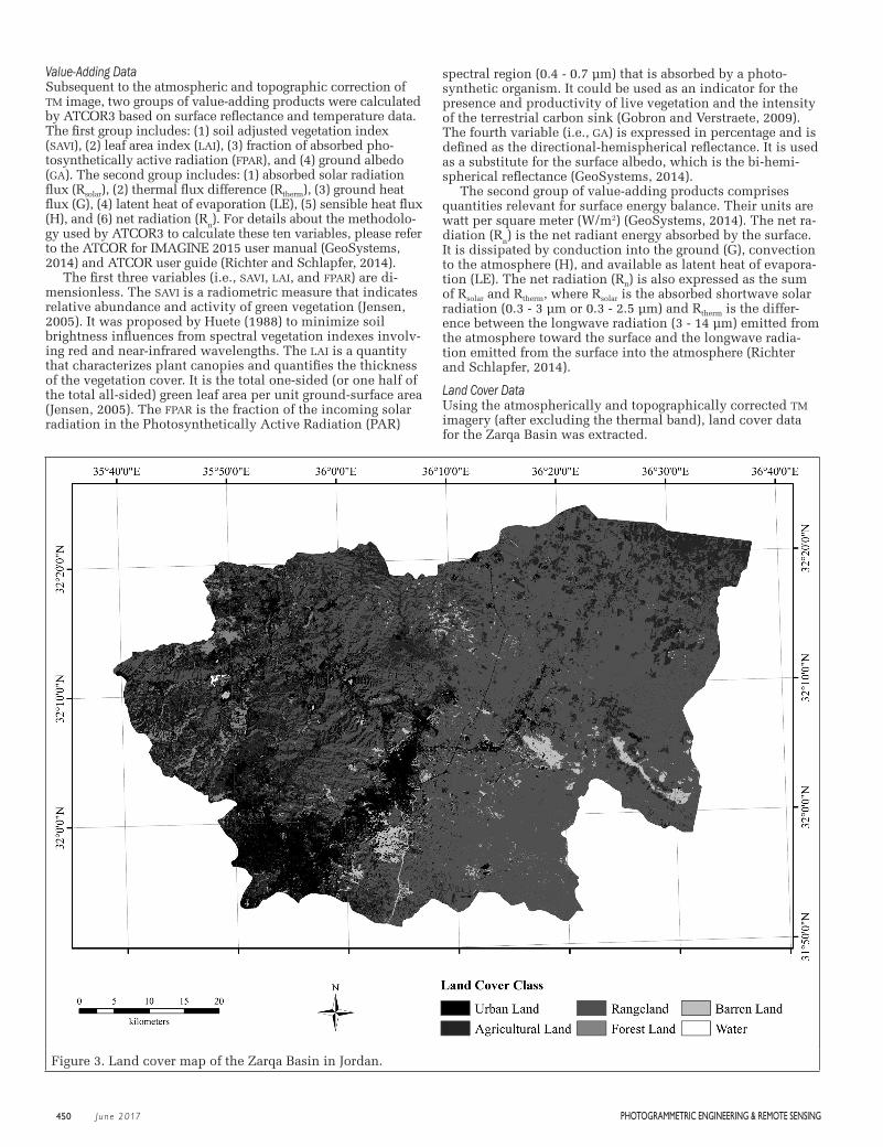
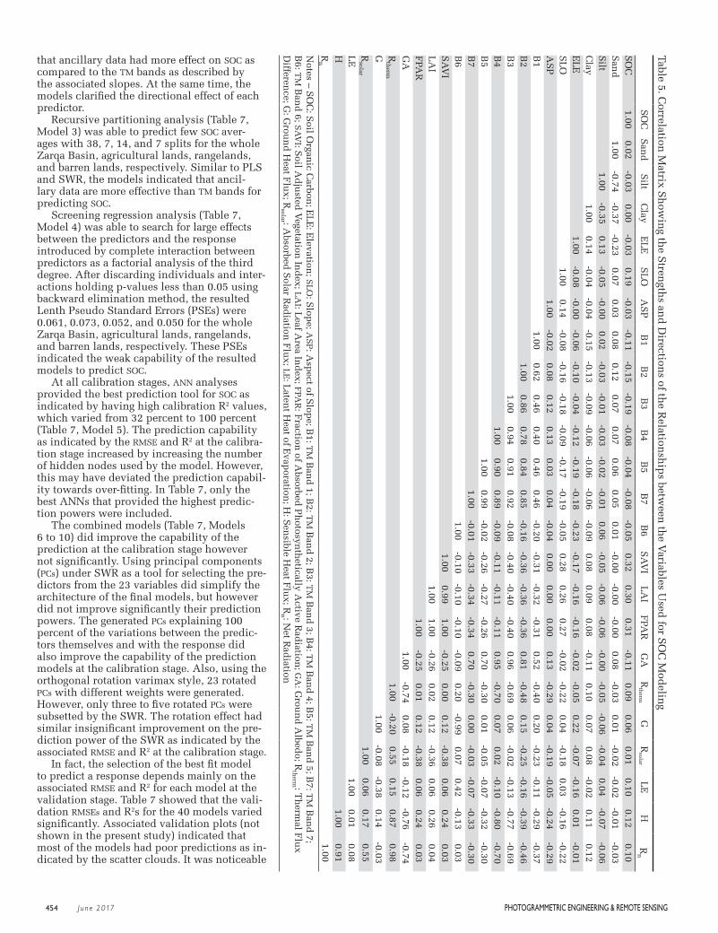
Land Cover DataUsing the atmospherically and topographically corrected TM imagery (after excluding the thermal band), land cover data for the Zarqa Basin was extracted.

Figure 3. Land cover map of the Zarqa Basin in Jordan.



First, based on personal experience in the field all land cover classes of interest were identified. These classes were: (1) Urban Land (UL), (2) Agricultural Land (AL), (3) Range-land (RL), (4) Forest Land (FL), (5) Barren Land (BL), and (6) Water (WA). The definitions of these classes were based upon the United States Geological Survey Land Use Land Cover Classification System (Anderson et al., 1976). Then, a total of 129 training sites were selected. In an iterative process, these training sites were evaluated and a total of 42 distinct signatures representing the six land cover classes were gener-ated. The spectral characteristics of these signatures were used to train a maximum likelihood supervised classification algorithm to classify the six-band atmospherically and topo-graphically corrected TM imagery into 42 land cover classes. Each class corresponds to a signature. Then, the 42 classes were combined into the six land cover classes of interest as described earlier. In order to remove the salt-and-pepper noise and enhance the quality and appearance of the resulted land cover thematic map, a 3 × 3-pixel majority spatial filter was applied. Finally, a total of 600 reference pixels were gener-ated following a stratified random sampling strategy in order to evaluate the accuracy of the resulted land cover thematic map by constructing an error matrix (Jensen, 2005) using the six land cover classes. The original image, ancillary data, and ground truthing were used to assess the accuracy of these reference pixels.

Soil Organic Carbon Modeling Analysis

Data ExplorationIn the present study, statistical modeling was applied to de-velop models that can be used to predict SOC (as a response) utilizing a combination of 23 variables (as predictors). These predictors represented some characteristics of the soil (i.e., Sand, Silt, and Clay), topography (i.e., Elevation (ELE), slope (SLO), and Aspect of Slope (ASP)), surface reflectance (i.e., TM band 1 (B1), TM band 2 (B2), TM band 3 (B3), TM band 4 (B4), TM band 5 (B5), and TM band 7 (B7)), surface brightness

temperature (i.e., TM band 6 (B6)), and value-adding products (i.e., SAVI, LAI, FPAR, GA, Rsolar, Rtherm, G, LE, H, and Rn).

However, before commencing with the modeling analy-sis, all the variables (i.e., dependent and independent) were examined using univariate and bivariate statistical measures. These measures included exploratory data analysis (EDA) using measures of central tendency, dispersion, and distribu-tion. The types, strengths, and directions of the relationships between all variables were investigated by applying correla-tion analysis using Pearson’s product moment correlation coefficient (r). Correlation analysis was useful for detecting the multi-collinearity, which is a crucial characteristic in the modeling process (Howell, 2013). The strengths of the relationships were classified into three levels: weak correla-tion when 0 ≤ |r| < 0.3, moderate correlation when 0.3 ≤ |r| < 0.7, and strong correlation when 0.7 ≤ |r| ≤ 1.0. In addition, comparison between means of SOC for all land cover types (except water) was applied using analysis of variance (ANO-VA) and Tukey-Kramer Honestly Significant Difference (HSD) test (Tukey, 1953; Kramer, 1956). The test represents an exact alpha-level test if the samples sizes are equal and conserva-tive if the samples sizes are different as the case in the present study (Hayter, 1984).

Calibration and Validation AnalysesSix major statistical modeling procedures were conducted. They are: (1) stepwise regression (SWR) (Mallows, 1973; Akaike, 1974; Montgomery et al., 2012), (2) partial least squares (PLS) (Wold, 1994; Turkmen and Billor, 2010), (3) recursive partitioning analysis (RPA) (Zhang and Singer, 2010), (4) screening regression analysis (SRA) (Campolongo et al., 2000; Wu and Hamada, 2000; Montgomery, 2005), (5) artificial neural networks (ANNs) (Samarasinghe, 2007), and (6) com-bined models (Rantanen et al., 2001; Ramadan et al., 2005). For a brief description of these procedures please see Table 1.

Although the above mentioned modeling procedures include least square or maximum likelihood tuning ap-proach, they were calibrated and validated using 75 percent

Table 1. Brief Description of the Modeling Procedures Implemented in Order to Develop Models for Predicting SOC

Modeling Procedure Description

Stepwise Regression Beginning with a model that included all the 23 predictors, the backward elimination procedure was used to remove the predictors that affected the model the least. Model calibration was based on Mallows’ Cp criterion and Akaikes Information Criterion (AIC).

Partial Least Squares This procedure was used to extract successive mutually independent linear combinations of the predictors (i.e., latent vectors) that provided maximum correlation with the response as suggested by the variable importance plot (VIP). The selection of latent vectors was based on percentage of variation explained for both Y variable and selected X variables. Four combined techniques were adopted for selection. They are VIP, score plots, diagnostic plots, and cross validation. The selection was based on significant percentage of variation explained providing a stable low root mean square error (RMSE) for the one-at-a-time method.

Recursive Partitioning Analysis

Tree of partitions (i.e., if-statements tree) for set of decision rules was performed using successive dataset splitting according to the relationships between SOC and the predictors.

Screening Regression Analysis

This procedure duplicates the theory of linear regression with complete interaction between predictors as a three-level design (i.e., factorial analysis of the third degree). It was formulated through calculating a t-ratio called Pseudo Standard Error (PSE) using the Lenth method.

Artificial Neural Networks

The most common form of artificial neural network (ANN), which is the feed-forward supervised learning back-propagation ANN, was tested for predicting SOC. Linear functions were used from the input layer of the 23 variables to the hidden layers and to the SOC output layer. A Sigmoidal (S-shape) activation function was used and one to twelve hidden nodes were tested.

Combined Models Combining stepwise regression (SWR) and/or principal components (PCs) (with and without rotational factors) with an ANN has several benefits, including orthogonalizing the components of the input vectors and eliminating those components that contribute the least to the variation in the data set. Therefore, the following combined models were tested:1. SWR applied for inputs selection of main PCs (both with and without rotational factors);2. SWR applied for inputs selection during ANN analysis with one to twelve hidden nodes; and3. SWR applied for inputs selection of main PCs (both with and without rotational factors) and then re-applied for

inputs selection in ANN analysis with one to twelve hidden nodes.



calibration and 25 percent validation sets of the soil samples, respectively, for the whole Zarqa Basin and for the different land cover types. The splitting into calibration and validation sets were random and repeated until both sets had almost similar statistical characteristics. All the models were tested using ANOVA with significance levels above 95 percent (i.e., p-values <0.05). Thus, using the validation sets, the predic-tion accuracies of the calibrated statistical models were evalu-ated according to the root mean square error (RMSE) and multi-ple coefficient of determination (R2). The model provided the lowest RMSE and highest R2 was considered to be the best.

Results and DiscussionBefore commencing with presenting the results of the pres-ent study, two issues represent precautionary measures worth mentioning. The first was that during conducting the fieldwork campaign, the composite soil samples were pro-cured from locations that represented the pixels of the TM imagery where they happened to exist. This evened out the short-range variability of SOC in every pixel and matched the supports of the dependent and independent variables. The second was that the chosen TM imagery was acquired on a date that coincided with time interval during which the field-work campaign was carried out in order to collect the neces-sary soil samples, which is very important for ensuring the potential correlation between the dependent and independent variables.

Topography and Land Cover of the Zarqa BasinTopography in the Zarqa Basin (Figure 2) varied greatly from about -198 m below mean sea level along the outlet of the Zarqa River in the west to about 1,241 m above mean sea level close to Salt City. In general, the eastern parts of the basin are relatively flat while the western parts are mountainous. Actu-ally, the Zarqa Basin is one of the transitional areas between the highlands in the west and the desert in the east.

Land cover mapping (Figure 3 and Table 2) showed that about 60 percent of the Zarqa Basin area is covered by range-lands, which dominate the eastern part of the basin. Urban and agricultural lands cover about 35 percent of the basin area. They dominate the western part of the basin where most of the capital city of Jordan (Amman) in addition to the Zarqa and Salt Cities lie. Barren lands constitute about 3 percent of the area of the basin. They exit mainly in the southeast. Forest lands cover about 2 percent of the area of the basin and exist mainly in the northwest. Water covers very small areas (about 0.03 percent) of the basin. Water is contained mainly in King Talal Dam in the west, Khirbit Al-Samrah Wastewater Treatment Plant in the middle, and the Zarqa River.

Table 3 shows the error matrix that was generated to assess the accuracy of the devel-oped land cover thematic map. The overall

accuracy of the map reached about 85.5 percent. Rangelands were found to have the highest user’s accuracy of about 97.9 percent with commission error of about 2.1 percent. Urban lands were found to have the highest producer’s accuracy of about 94.0 percent with omission error of about 6.0 percent. However, the lowest user’s accuracy was calculated for the urban lands of about 64.5 percent with commission error of about 35.5 percent and the lowest producer’s accuracy was calculated for the water class of about 71.4 percent with omis-sion error of about 28.6 percent.

Characteristics of the Dependent and Independent Variables in the Zarqa BasinTable 4 shows some basic descriptive statistics of the depen-dent and independent variables used in the present study. All the variables appeared to be highly dispersed as indicated by their high standard deviations and high coefficients of varia-tions. This high variability could be attributed to many factors including natural and human induced. Soil properties, land cover, and topography, in addition to human activities (e.g., land use and land management practices) are variables that have high heterogeneity within the study area, which could affect the spatial variability of these variables. In general, Zar-qa Basin soils are poorly aggregated and mostly calcareous, associated with high gravel and stone contents, and subjected to varying crust formations (Al-Qinna et al., 2008).

Normality testing using Shapiro-Wilk W Test indicated that SOC had log-normal distribution, thus the SOC data were transformed into logarithmic form, while the predictors var-ied with regard to their distributions from normal to logarith-mic to power (Table 4). This indicated heterogeneities of the distributions of these variables, which were reflected in their capabilities to be used in the modeling analysis in both cali-bration and validation stages and eventually the accuracies of predictions. In addition, high skewness and kurtosis of some of the predictors were noticed (e.g., SLO, B1, LAI, and LE), which could be explained by the presence of outliers.

Correlation analysis (Table 5) shows the presence of weak to moderate relationships between SOC (as a response) and the 23 variables (as predictors). Pearson’s product moment correlation coefficient (r) varied from 0.00 (between Clay and SOC) to 0.32 (between SAVI and SOC). This created additional difficulties during the development of representative statisti-cal prediction models.

Moreover, strong relationships were found between the TM bands themselves and between the value-adding products

Table 2. Land Cover Classes Developed for the Zarqa Basin and Their Coverage Areas and Percentages

Land Cover Class Area (km2) Area (%)

Urban Land 669.641 18.687

Agricultural Land 569.398 15.890

Rangeland 2154.469 60.123

Forest Land 77.802 2.171

Barren Land 111.023 3.098

Water 1.111 0.031

Total 3583.444 100.000

Table 3. The Error Matrix Associated with the Developed Land Cover Thematic Map for the Zarqa Basin

Reference DataRow Total

User’s Accuracy

(%)

Commission Error (%)UL AL RL FL BL WA

Cla

ssifi

ed D

ata

UL 78 6 32 1 2 2 121 64.46 35.54

AL 0 89 13 1 0 0 103 86.41 13.59

RL 1 4 275 0 1 0 281 97.86 2.14

FL 0 3 2 20 0 4 29 68.97 31.03

BL 4 0 6 0 36 0 46 78.26 21.74

WA 0 3 0 2 0 15 20 75.00 25.00

Column Total

83 105 328 24 39 21 600

Producer’s Accuracy (%)

93.98 84.76 83.84 83.33 92.31 71.43

Omission Error (%)

6.02 15.24 16.16 16.67 7.69 28.57

Overall Accuracy = 85.50%

Notes – UL: Urban Land; AL: Agricultural Land; RL: Rangeland; FL: Forest Land; BL: Barren Land; WA: Water



themselves. In addition, strong relationships were noticed between the TM bands and GA and between B6 and G. These strong correlations indicated the presence of multi-collinear-ity among the predictors, thus providing redundant informa-tion, which added more challenge during the development of the predictive models. The multi-collinearity among the predictors were removed through adopting the suitable meth-odologies of variable selection for each modeling procedure. They included backward elimination, variable importance plot (VIP), score plots, diagnostics plots, and cross validation tests (Table 1).

Furthermore, all the variables varied significantly with regard to land cover type (Table 6). The highest SOC mean was found in forest lands (about 54.9 ton/ha) while the lowest mean was associated with barren lands (about 12.7 ton/ha). Similarly, satellite-based predictors varied significantly with land cover type, which is true since they represent reflectance of the surface, which vary by land cover type.

Soil Organic Carbon Modeling AnalysisTable 7 provided the results obtained from both the calibration and validation stages for the 40 models applied after natural logarithm transformation of SOC in the whole Zarqa Basin and in agricultural lands, rangelands, and barren lands. The modeling analysis was performed for all land cover types that exist in the Zarqa Basin, except urban and forest lands; the samples’ sizes associated with urban and forest lands (36 for urban lands and 21 for forest land) were relatively small and hindered the modeling analysis in these two land cover types.

The backward-selection criterion in SWR analysis, which is based on Akaike’s Information Criterion and Mallow’s Cp

criterion at 5 percent significance probability level (p-value), was able to subset the whole 23-predictor models into models with less than seven predictors (Equations 1 to 4) (Table 7, Model 1). The generated models reduced the multi-collinear-ity among the predictors. Depending on the land cover class, the generated models had different combinations of predic-tors.

For the whole Zarqa Basin: Log(SOC) = 3.119 + 0.057 × B1 – 0.127 × B3 + 0.072 B5 – 3.070 × LAI – 0.048 × Rsolar + 0.016 × Rn

(1)

For the agricultural lands: Log(SOC) = 0.399 + 0.244 × B2 + 0.457 × B5 + 11.153 × FPAR – 0.685 × GA + 0.011 Rsolar

(2)

For the rangelands: Log(SOC) = 3.208 + 0.077 × B1 – 0.112 × B3 + 0.063 × B7 + 0.027 Rtherm + 0.044 G – 0.022 Rsolar – 0.031 × H

(3)

For the barren lands: Log(SOC) = 0.526 + 0.021× B4 + 0.004 × H (4)

Out of 15 latent vectors representing the 23 variables gen-erated using the PLS method, only the first three to four vec-tors were selected and used in retreating the SOC prediction models had the most cumulative explanations in SOC (Table 7, Model 2). The selected latent vectors were able to explain 79 percent, 81 percent, 86 percent, and 88 percent for the Whole Zarqa Basin, Agricultural Lands, Barren Lands, and Range-lands, respectively. However, all generated models indicated

Table 4. Some Descriptive Statistics of the Variables Used in the Modeling Analysis

Variable Minimum Maximum MeanStandardDeviation Skewness Kurtosis

Coefficient of Variation (%)

DistributionType

SOC (ton/ha) 4.83 83.75 24.93 14.92 1.43 2.21 59.82 Logarithmic

Sand (%) 0.00 86.20 54.00 7.40 -0.66 11.87 13.72 Power

Silt (%) 1.30 100.00 33.80 7.35 1.93 21.49 21.76 Power

Clay (%) 0.00 30.20 12.30 5.33 0.23 0.30 43.44 Normal

ELE (m) 267.00 1050.00 666.10 124.22 0.20 0.53 18.65 Normal

SLO (°) 0.48 89.91 6.94 6.31 7.36 91.05 90.88 Power

ASP (°) 0.00 358.45 174.24 103.19 0.05 1.10 59.22 Normal

B1 (%) 0.10 88.30 7.72 6.03 7.65 100.30 78.16 Power

B2 (%) 2.30 41.90 18.27 6.46 -0.05 41.67 35.33 Normal

B3 (%) 0.10 45.30 22.35 8.10 -0.45 0.49 36.24 Normal

B4 (%) 0.10 64.10 35.53 10.54 -0.84 2.23 29.66 Normal

B5 (%) 0.10 65.10 36.85 11.84 -0.87 1.36 32.14 Normal

B7 (%) 0.10 55.00 30.75 10.33 -0.87 1.14 33.59 Normal

B6 (°C) 0.00 25.10 17.72 2.74 -1.87 10.82 15.45 Power

SAVI 0.12 0.46 0.19 0.04 2.39 9.60 20.88 Power

LAI 0.05 1.32 0.25 0.13 3.29 18.48 52.78 Power

FPAR 0.02 0.41 0.09 0.04 2.64 11.85 47.38 Power

GA (%) 8.40 55.80 31.67 8.73 -0.27 0.03 27.57 Normal

Rtherm (W/m2) 24.00 616.00 422.63 83.06 -0.64 1.56 19.65 Power

G (W/m2) 0.00 114.00 28.62 13.99 1.70 8.22 48.89 Power

Rsolar (W/m2) 0.00 202.00 135.00 33.46 -1.75 5.64 24.79 Power

LE (W/m2) 0.00 13.000 0.31 1.54 6.15 40.34 496.24 Power

H (W/m2) 41.00 615.00 325.33 68.93 0.44 3.10 21.19 Power

Rn (W/m2) 54.00 641.00 451.08 81.30 -0.61 1.66 18.03 Power

Notes – SOC: Soil Organic Carbon; ELE: Elevation; SLO: Slope; ASP: Aspect of Slope; B1: TM Band 1; B2: TM Band 2; B3: TM Band 3; B4: TM Band 4; B5: TM Band 5; B7: TM Band 7; B6: TM Band 6; SAVI: Soil Adjusted Vegetation Index; LAI: Leaf Area Index; FPAR: Fraction of Ab-sorbed Photosynthetically Active Radiation; GA: Ground Albedo; Rtherm: Thermal Flux Difference; G: Ground Heat Flux; Rsolar: Absorbed Solar Radiation Flux; LE: Latent Heat of Evaporation; H: Sensible Heat Flux; Rn: Net Radiation



that ancillary data had more effect on SOC as compared to the TM bands as described by the associated slopes. At the same time, the models clarified the directional effect of each predictor.

Recursive partitioning analysis (Table 7, Model 3) was able to predict few SOC aver-ages with 38, 7, 14, and 7 splits for the whole Zarqa Basin, agricultural lands, rangelands, and barren lands, respectively. Similar to PLS and SWR, the models indicated that ancil-lary data are more effective than TM bands for predicting SOC.

Screening regression analysis (Table 7, Model 4) was able to search for large effects between the predictors and the response introduced by complete interaction between predictors as a factorial analysis of the third degree. After discarding individuals and inter-actions holding p-values less than 0.05 using backward elimination method, the resulted Lenth Pseudo Standard Errors (PSEs) were 0.061, 0.073, 0.052, and 0.050 for the whole Zarqa Basin, agricultural lands, rangelands, and barren lands, respectively. These PSEs indicated the weak capability of the resulted models to predict SOC.

At all calibration stages, ANN analyses provided the best prediction tool for SOC as indicated by having high calibration R2 values, which varied from 32 percent to 100 percent (Table 7, Model 5). The prediction capability as indicated by the RMSE and R2 at the calibra-tion stage increased by increasing the number of hidden nodes used by the model. However, this may have deviated the prediction capabil-ity towards over-fitting. In Table 7, only the best ANNs that provided the highest predic-tion powers were included.

The combined models (Table 7, Models 6 to 10) did improve the capability of the prediction at the calibration stage however not significantly. Using principal components (PCs) under SWR as a tool for selecting the pre-dictors from the 23 variables did simplify the architecture of the final models, but however did not improve significantly their prediction powers. The generated PCs explaining 100 percent of the variations between the predic-tors themselves and with the response did also improve the capability of the prediction models at the calibration stage. Also, using the orthogonal rotation varimax style, 23 rotated PCs with different weights were generated. However, only three to five rotated PCs were subsetted by the SWR. The rotation effect had similar insignificant improvement on the pre-diction power of the SWR as indicated by the associated RMSE and R2 at the calibration stage.

In fact, the selection of the best fit model to predict a response depends mainly on the associated RMSE and R2 for each model at the validation stage. Table 7 showed that the vali-dation RMSEs and R2s for the 40 models varied significantly. Associated validation plots (not shown in the present study) indicated that most of the models had poor predictions as in-dicated by the scatter clouds. It was noticeable

Table 5. Correlation

Matrix S

how

ing th

e Stren

gths an

d D

irections of th

e Relation

ship

s between

the V

ariables Used

for SO

C M

odelin

g

SO

CS

and

Silt

Clay

EL

ES

LO

AS

PB

1B

2B

3B

4B

5B

7B

6S

AV

IL

AI

FPA

RG

AR

therm

GR

solarL

EH

Rn

SO

C1.00

0.02-0.03

0.00-0.03

0.19-0.03

-0.11-0.15

-0.19-0.08

-0.04-0.08

-0.050.32

0.300.31

-0.110.09

0.060.01

0.100.12

0.10S

and

1.00-0.74

-0.37-0.23

0.070.03

0.080.12

0.070.07

0.060.05

0.01-0.00

-0.00-0.00

0.08-0.03

0.01-0.02

-0.02-0.01

-0.03S

ilt1.00

-0.350.13

-0.05-0.00

0.02-0.03

-0.01-0.03

-0.02-0.01

0.06-0.05

-0.06-0.06

-0.00-0.05

-0.06-0.04

0.04-0.07

-0.06C

lay1.00

0.14-0.04

-0.04-0.15

-0.13-0.09

-0.06-0.06

-0.06-0.09

0.080.09

0.08-0.11

0.100.07

0.08-0.02

0.110.12

EL

E1.00

-0.08-0.00

-0.06-0.10

-0.04-0.12

-0.19-0.18

-0.23-0.17

-0.16-0.16

-0.02-0.05

0.22-0.07

-0.160.01

-0.01S

LO

1.000.14

-0.08-0.16

-0.18-0.09

-0.17-0.19

-0.050.28

0.260.27

-0.02-0.22

0.04-0.18

0.03-0.16

-0.22A

SP

1.00-0.02

0.080.12

0.130.03

0.04-0.04

0.000.00

0.000.13

-0.290.04

-0.19-0.05

-0.24-0.29

B1

1.000.62

0.460.40

0.460.46

-0.20-0.31

-0.32-0.31

0.52-0.40

0.20-0.23

-0.11-0.29

-0.37B

21.00

0.860.78

0.840.85

-0.16-0.36

-0.36-0.36

0.81-0.48

0.15-0.25

-0.16-0.39

-0.46B

31.00

0.940.91

0.92-0.08

-0.40-0.40

-0.400.96

-0.690.06

-0.02-0.13

-0.77-0.69

B4

1.000.90

0.89-0.09

-0.11-0.11

-0.110.95

-0.700.07

0.02-0.10

-0.80-0.70

B5

1.000.99

-0.02-0.26

-0.27-0.26

0.70-0.30

0.01-0.05

-0.07-0.32

-0.30B

71.00

-0.01-0.33

-0.34-0.34

0.70-0.30

0.00-0.03

-0.07-0.33

-0.30B

61.00

-0.10-0.10

-0.10-0.09

0.20-0.99

0.070.42

-0.130.03

SA

VI

1.000.99

1.00-0.25

0.000.12

-0.380.06

0.240.03

LA

I1.00

1.00-0.26

0.020.12

-0.360.06

0.260.04

FPA

R1.00

-0.250.01

0.12-0.38

0.060.24

0.03G

A1.00

-0.740.08

-0.18-0.12

-0.76-0.74

Rth

erm1.00

-0.200.55

0.150.87

0.98G

1.00-0.08

-0.380.14

-0.03R

solar1.00

0.060.17

0.55L

E1.00

0.010.08

H1.00

0.91R

n1.00

Notes – S

OC

: Soil O

rganic C

arbon; E

LE

: Elevation

; SL

O: S

lope; A

SP: A

spect of S

lope; B

1: TM

Ban

d 1; B

2: TM

Ban

d 2; B

3: TM

Ban

d 3; B

4: TM

Ban

d 4; B

5: TM

Ban

d 5; B

7: TM

Ban

d 7;

B6: T

M B

and

6; SA

VI: S

oil Ad

justed

Vegetation

Ind

ex; LA

I: Leaf A

rea Ind

ex; FPA

R: F

raction of A

bsorbed P

hotosyn

thetically A

ctive Rad

iation; G

A: G

roun

d A

lbedo; R

therm : T

herm

al Flu

x D

ifference; G

: Grou

nd

Heat F

lux; R

solar : Absorbed

Solar R

adiation

Flu

x; LE: L

atent H

eat of Evap

oration; H

: Sen

sible Heat F

lux; R

n : Net R

adiation



that most of the models provided inadequacy in predicting SOC through showing extreme biased predictions especially at very low or high SOC values, where all the models tended to over-predict SOC at low values and under-predict SOC at high values. This could be explained theoretically by having weak correlations between SOC and the 23 predictors.

The RPA was inconvenient in its prediction methodology since it predicted only equivalent number of splits. The errors associated with the SRA were relatively high as indicated by RMSE values, in addition to the low R2 values. Similarly, all combined models associated with PCs were rejected due to as-sociated high errors and low correlations as indicated by their associated RMSEs and R2.

Overall, the selection of best models (i.e., between SWR, PLS, ANN, and ANN(SWR)) depends on the land cover class. In most cases, the ANN models were almost the best models to predict SOC under various land cover classes. However precautions should be taken during using ANN for extrapola-tions. The ANN is set as a black box where the weights change with respect to input-output behavior during training and use of trained system to generate correct outputs using the weights. Thus, the models should be periodically monitored and improved.

Table 6. Comparison between Means of SOC for All Land Cover Types (Except Water) Using Analysis of Variance (ANOVA) and Tukey-Kramer Honestly Significant Difference (HSD) Test

VariableUrban Land

Agricultural Land Rangeland

Forest Land

Barren Land

SOC (ton/ha) 27.10 bc 30.74 b 23.12 c 54.86 a 12.69 d

Sand (%) 53.40 a 52.14 a 54.61 a 56.64 a 54.37 a

Silt (%) 33.12 a 34.48 a 33.50 a 33.00 a 33.97 a

Clay (%) 13.49 a 13.38 a 11.89 a 10.37 a 11.66 a

ELE (m) 675.69 a 677.33 a 670.68 a 660.67 a 644.58 a

SLO (°) 6.44 ab 7.63 ab 6.66 b 11.10 a 5.80 b

ASP (°) 150.68 a 172.89 a 182.77 a 159.07 a 177.47 a

B1 (%) 8.60 ab 5.41 b 8.06 a 5.79 ab 9.54 a

B2 (%) 19.19 a 13.92 b 19.82 a 14.38 b 20.83 a

B3 (%) 23.88 a 17.26 b 24.02 a 17.03 b 25.51 a

B4 (%) 36.24 a 30.34 b 37.24 a 32.24 ab 38.53 a

B5 (%) 37.81 ab 31.06 c 38.00 ab 32.92 bc 41.43 a

B7 (%) 31.98 ab 25.36 c 31.91 ab 26.19 bc 34.99 a

B6 (°C) 17.55 ab 17.96 ab 17.64 ab 16.15 b 18.12 a

SAVI 0.18 c 0.20 b 0.18 c 0.23 a 0.17 c

LAI 0.22 c 0.30 b 0.22 c 0.39 a 0.20 c

FPAR 0.08 c 0.11 b 0.085 c 0.14 a 0.08 c

GA (%) 31.94 ab 26.94 c 33.67 a 27.09 bc 34.37 a

Rtherm (W/m2) 421.08 ab 451.62 a 406.19 b 439.29 ab 415.71 ab

G (W/m2) 29.39 ab 27.64 b 28.90 ab 37.48 a 26.36 b

Rsolar (W/m2) 135.69 a 140.80 a 131.04 a 134.57 a 135.25 a

LE (W/m2) 0.53 ab 0.83 a 0.08 b 0.52 ab 0.00 b

H (W/m2) 324.00 ab 346.34 a 313.48 b 357.05 ab 314.91 b

Rn (W/m2) 450.22 ab 478.82 a 435.09 b 476.10 ab 442.07 b

Notes – Levels not connected by same letter are significantly different at 95% confidence level.SOC: Soil Organic Carbon; ELE: Elevation; SLO: Slope; ASP: Aspect of Slope; B1: TM Band 1; B2: TM Band 2; B3: TM Band 3; B4: TM Band 4; B5: TM Band 5; B7: TM Band 7; B6: TM Band 6; SAVI: Soil Adjusted Vegetation Index; LAI: Leaf Area Index; FPAR: Fraction of Absorbed Photosynthetically Active Radiation; GA: Ground Albedo; Rtherm: Thermal Flux Difference; G: Ground Heat Flux; Rsolar: Absorbed Solar Radiation Flux; LE: Latent Heat of Evaporation; H: Sensible Heat Flux; Rn: Net Radiation

Table 7. Calibration

and

Valid

ation S

tatistics of the M

odels th

at were D

eveloped

for Mod

eling S

OC A

fter Ap

plyin

g Natu

ral Logarith

m Tran

sformation

in th

e Wh

ole Z

arqa Basin

, agricultu

ral land

s, rangelan

ds, an

d barren

land

s

No.

Mod

el

Wh

ole Zarqa B

asinA

gricultu

ral Lan

dR

angelan

dB

arren L

and

Calibration

Valid

ationC

alibrationV

alidation

Calibration

Valid

ationC

alibrationV

alidation

RM

SE

R2

RM

SE

R2

RM

SE

R2

RM

SE

R2

RM

SE

R2

RM

SE

R2

RM

SE

R2

RM

SE

R2

1S

WR

0.5030.2622

0.5180.1581

0.3930.3648

0.4330.1995

0.3270.2408

0.4440.0203

0.3520.1136

0.4140.0694

2P

LS

0.4890.3024

0.5470.1022

0.3590.4707

0.4420.1971

0.3220.2716

0.4150.0495

0.3020.3605

0.5510.0199

3R

PA0.304

0.7290.721

0.00580.312

0.60060.582

0.03960.228

0.63250.437

0.01580.229

0.63170.484

0.09334

SR

A0.515

0.22540.573

0.02580.430

0.23320.861

0.04720.359

0.08560.441

0.03450.332

0.21150.397

0.14445

AN

N0.482

0.32190.558

0.08780.149

0.90900.513

0.06260.023

0.99650.567

0.11870.291

0.40510.452

0.09316

SW

R(P

C)

0.5520.1115

0.5560.0174

0.4710.0879

0.4250.0575

0.3760.0076

0.4130.0414

0.3810.0187

0.4330.0517

7S

WR

(RP

C)

0.5520.1099

0.5590.0125

0.4780.0608

0.4320.0277

0.3750.0132

0.4150.0398

0.3770.0015

0.4340.0563

8A

NN

(SW

R)

0.5030.2620

0.5180.1565

0.3930.3672

0.4160.2120

0.3180.2802

0.4340.0037

0.3280.2278

0.4170.0940

9A

NN

(SW

R(P

C))

0.5320.1722

0.5620.0317

0.4570.1418

0.4260.0586

0.3720.0262

0.4050.0010

0.3690.04000

0.4310.0356

10A

NN

(SW

R(R

PC

))0.534

0.16810.569

0.02500.455

0.14820.421

0.05510.360

0.08900.406

0.01450.369

0.04010.439

0.0463

Notes – S

WR

: Step

wise R

egression; P

LS

: Partial L

east Squ

ares; RPA

: Recu

rsive Partition

ing A

nalysis; S

RA

: Screen

ing R

egression A

nalysis; A

NN

: Artifi

cial Neu

ral Netw

ork; PC

: Prin

-cip

al Com

pon

ent; S

WR

(PC

): Com

bined

Mod

el of SW

R of th

e PC

s; SW

R(R

PC

): Com

bined

Mod

el of SW

R of th

e Rotated

PC

s; AN

N(S

WR

): Com

bined

Mod

el of AN

N of S

WR

outp

uts;

AN

N(S

WR

(PC

)): Com

bined

Mod

el of AN

N of (S

WR

of (PC

)) outp

uts; A

NN

(SW

R(R

PC

)): Com

bined

Mod

el of AN

N of (S

WR

of (RP

C)) ou

tpu

ts; RM

SE

: Root M

ean S

quare E

rror, R2: M

ultip

le C

oefficien

t of Determ

ination

.



Applicability of the Developed Models in Carbon Crediting ProgramsSo, is it possible to use the developed SOC models in the present study for implementing carbon crediting programs in semi-arid environments? Following the procedure adopted by Jaber and Al-Qinna (2011), comparing the smallest RMSE associated with the developed models for the whole Zarqa Basin of about 1.679 ton/ha to the mean decadal scale carbon sequestration rates due to changes in farming practices, as reported by West and Post (2002), indicated that the ratios ob-tained varied from 18.0 percent to 118.2 percent for a change from conventional tillage to no-till and from 31.2 percent to 161.4 percent for enhancement of crop rotation complexity. Breaking down the comparisons by land cover type showed that the best results were obtained in barren lands (smallest RMSE equals 1.487 ton/ha) followed by rangelands (smallest RMSE equals 1.499 ton/ha) then agricultural lands (small-est RMSE equals 1.516 ton/ha). The ratios obtained in barren lands varied from 16.0 percent to 104.7 percent for a change from conventional tillage to no-till and from 27.6 percent to 143.0 percent for enhancement of crop rotation complexity. In rangelands the ratios obtained varied from 16.1 percent to 105.6 percent for a change from conventional tillage to no-till and from 27.9 percent to 144.1 percent for enhance-ment of crop rotation complexity. While in agricultural lands the ratios obtained varied from 16.3 percent to 106.8 percent for a change from conventional tillage to no-till and from 28.2 percent to 145.8 percent for enhancement of crop rota-tion complexity. Although these margins of errors indicate significant enhancements to the ones obtained by previous studies such as Jaber and Al-Qinna (2011) of about 10.4 ton/ha using Landsat-5 TM data, Were et al. (2015) of about 14.9 ton/ha using Landsat-8 OLI data, and Winowiecki et al. (2016) of about 9 to 10.3 ton/ha using MODIS data, they are still relatively high. This means that the developed SOC models in the present study still cannot be used for direct application in applying and monitoring carbon crediting programs in semi-arid environments.

This could be attributed to the following factors. (a) The spectral information content of many of the TM pixels is not directly related to the soil and also not pure but is a mixture of different land cover types. (b) There is huge variability of SOC in the study area. Actually, SOC content in semi-arid areas is hypothesized to be of low magnitude, however, the pres-ence of high magnitudes were induced by human activities, such as variations in land management practices especially rate and frequency of manure applications, in addition to natural variations, such as soil type, topography, and land cover. (c) Uncertainties associated with the auxiliary data and personal errors in soil sampling and laboratory analysis can-not be ruled out.

Conclusions and RecommendationsThe present study led to the following main conclusions. (1) Land cover was found to be a major factor that affected the modeling analyses for SOC (i.e., the algorithms developed and the predictors included varied significantly according to the land cover class). (2) The modeling analyses for SOC in the agricultural lands produced relatively better results if compared with those obtained in rangelands and barren lands and in the whole Zarqa Basin. This is surely not attribut-able to the samples’ sizes since rangelands (and of course the whole Zarqa Basin) had larger sampling data points as compared to the other land cover classes. However, it was clear that the correlations between SOC and the 23 variables were relatively larger in the agricultural lands if compared with those obtained in the other land cover classes and in the whole basin. (3) Barren lands had simpler prediction models

since they had less SOC variability as compared to the other land cover types and the whole basin. (4) Auxiliary data were found to be more important than TM data for predicting SOC. (5) Although none of the developed models was powerful in predicting SOC, ANN models were more applicable specifically in agricultural lands. (6) The margins of errors associated with the best models were relatively high and thus these models cannot be used for direct application in applying and moni-toring carbon crediting programs in semi-arid environments.

Hence, (a) using other variables that might affect the ac-cumulation and decomposition of organic carbon in the soil, such as moisture regime, temperature regime, soil order, soil aeration, nitrogen content, carbonate content, salt content, and gravel content, in addition to historical emphasis for land management (such as tillage practice, rate of organic matter addition, and organic matter type); (b) applying spatially ex-plicit modeling techniques, such as geographically weighted regression and regression kriging; and (c) downscaling the analyses to more detailed land cover classes, such as differ-ent types of agricultural lands (e.g., croplands, pasture, and orchards) and rangelands (e.g., herbaceous rangelands and shrubs) and barren lands (e.g., bare exposed rocks and mixed barren lands), might result in developing models with better accuracies acceptable to be used for implementing carbon crediting programs in semi-arid environments. These recom-mendations might be the concepts for future potential related studies.

AcknowledgmentsThis material is based upon work supported by the Dean-ship of Scientific Research of the Hashemite University in the Hashemite Kingdom of Jordan. The grant title is ‘Estimat-ing Surface Soil Organic Carbon Content in the Zarqa Basin, Jordan, Using Multispectral Data and Map Algebra.’

ReferencesAgbu, P.A., D.J. Fehrenbacher, and I.J. Jansen, 1990. Soil property

relationships with SPOT satellite digital data in east central Illinois, Soil Science Society of America Journal, 54:807–812.

Akaike, H., 1974. A new look at the statistical model identification, IEEE Transactions on Automatic Control, 19:716–723.

Al-Qinna, M., M. Salahat, and Z. Shatnawi, 2008. Effects of carbonates and gravel contents on hydraulic properties in gravely-calcareous soils, Dirasat, Agriculture Science, 35:145–158.

Anderson, J.R., E.E. Hardy, J.T. Roach, and R.E. Witmer, 1976. A Land Use and Land Cover Classification System for Use with Remote Sensor Data, Geological Survey Professional Paper 964, A Revision of the Land Use Classification System as presented in US Geological Survey Circular 671, United States Government Printing Office, Washington, D.C.

Blake, G.R., and K.H. Hartge, 1986. Bulk density, Methods of Soil Analysis: Part 1 – Physical and Mineralogical Methods, American Society of Agronomy, Inc., and Soil Science Society of America, Inc., pp. 363–375.

Bolstad, P., 2012. GIS Fundamentals: A First Text on Geographic Information Systems, Eider Press.

Campolongo, F., J.P.C. Kleijnen, and T. Andres, 2000. Screening methods, Sensitivity Analysis (A. Saltelli, K. Chan, and E.M. Scott, editors), John Wiley and Sons, Inc., pp. 65–89.

Esri, 2012. ArcGIS Desktop Help, Esri, Inc.Gee, G.W., and R.H. Bauder, 1986. Particle-size analysis, Methods of

Soil Analysis (A. Klute, editor), ASA, USA, pp. 383–411.GeoSystems, 2014. ATCOR for IMAGINE 2015: Haze Reduction,

Atmospheric and Topographic Correction, User Manual, ATCOR 2 and ATCOR 3, GeoSystems GmbH, Germany.



Gobron, N., and M.M. Verstraete, 2009. FAPAR: Fraction of Absorbed Photosynthetically Active Radiation (FAPAR), Assessment of the Status of the Development of the Standards for the Terrestrial Essential Climate Variables, GTOS Secretariat, NRC, Food and Agriculture Organization of the United Nations (FAO), Italy.

Grossman, R.B., and T.G. Reinsch, 2002. Bulk density and linear extensibility, Methods of Soil Analysis: Part 4 (J.H. Dane and G.C. Topp, editors), Soil Science Society of America, Inc. and American Society of Agronomy, Inc., pp. 201-228.

Hayter, A.J. 1984. A proof of conjecture that the Tukey-Kramer multiple comparisons procedure is conservative, Annals of Mathematical Statistics, 12:61–75.

Howell, D.C., 2013. Statistical Methods for Psychology, Wadsworth Publishing Company.

Huete, A.R., 1988. A soil-adjusted vegetation index (SAVI), Remote Sensing of Environment, 25:295–309.

IPCC, 2007a. Summary for policymakers, Climate Change 2007: The Physical Science Basis, Contribution of Working Group I to the Fourth Assessment Report of the Intergovernmental Panel on Climate Change, Cambridge University Press, UK.

IPCC, 2007b. Summary for policymakers, Climate Change 2007: Impacts, Adaptation, and Vulnerability, Contribution of Working Group II to the Fourth Assessment Report of the Intergovernmental Panel on Climate Change, Cambridge University Press, UK.

IPCC, 2007c. Summary for policymakers, Climate Change 2007: Mitigation, Contribution of Working Group III to the Fourth Assessment Report of the Intergovernmental Panel on Climate Change, Cambridge University Press, UK.

Jaber, S.M., and Al-Qinna, M.I., 2015. Global and local modeling of soil organic carbon using Thematic Mapper data in a semi-arid environment, Arabian Journal of Geosciences, 8:3159–3169.

Jaber, S.M., and Al-Qinna, M.I., 2011. Soil organic carbon modeling and mapping in a semi-arid environment using Thematic Mapper data, Photogrammetric Engineering & Remote Sensing, 77(6):709–719.

Jensen, J.R., 2005. Remote Sensing of the Environment: An Earth Resource Perspective, Pearson Prentice Hall.

Kramer, C.Y., 1956. Extension of multiple range tests to group means with unequal numbers of replications, Biometrics, 12:309–310.

Ladoni, M., S.K. Alavipanah, H.A. Bahrami, and A.A. Noroozi, 2010. Remote sensing of soil organic carbon in semi-arid region of Iran, Arid Land Research and Management, 24:271–281.

Lal, R., 2008. Carbon sequestration, Philosophical Transactions of the Royal Society B, 363:815–830.

LP DAAC, 2014. Land processes distributed active archive center, United States Geological Survey, URL: https://lpdaac.usgs.gov/dataset_discovery/aster/aster_products_table (last date accessed: 01 May 2017).

Mallows, C.L., 1973. Some comments on Cp, Technometrics, 15:661–675.MOE, 2013. The National Climate Change Policy of the Hashemite

Kingdom of Jordan 2013-2010, Ministry of Environment of Jordan, Supported by Global Environment Facility (GEF) and United Nations Development Program (UNDP).

MOE, 2009. Jordan’s Second National Communication to the United Nations Framework Convention on Climate Change (UNFCCC) 2009, Ministry of Environment of Jordan.

Montgomery, D.C., 2005. Design and Analysis of Experiments, John Wiley and Sons, Inc.

Montgomery, D.C., E.A. Peck, and G.G. Vining, 2012. Introduction to Linear Regression Analysis, John Wiley and Sons, Inc.

Moseley, J., and W. Richards, 2007. Foreword, Soil Carbon Management: Economic, Environmental, and Societal Benefits (J.M. Kimble, C.W. Rice, D. Reed, S. Mooney, R.F. Follett, and R. Lal, editors), CRC Press.

NASA, 2016. Landsat then and now, NASA, URL: http://landsat.gsfc.nasa.gov/about/ (last date accessed: 01 May 2017).

Nelson, D.W., and L.E. Sommers, 1996. Total carbon, organic carbon, and organic matter, Methods of Soil Analysis, Part 3, Chemical Methods, Soil Science Society of America, Inc. and American Society of Agronomy, Inc., pp. 961–1010.

Poggio, L., and A. Gimona, 2014. National scale 3D modeling of soil organic carbon stocks with uncertainty propagation - An example from Scotland, Geoderma, 232–234: 284–299.

Peng, Y., X. Xiong, K. Adhikari, M. Knadel, S. Grunwald, and M.H. Greve, 2015. Modeling soil organic carbon at regional scale by combining multi-spectral images with laboratory spectra, PLoS ONE, 10(11): e0142295. doi: 10.1371/journal.pone.0142295

Ramadan, Z., P.K. Hopke, M.J. Johnson, and K.M. Scow, 2005. Application of PLS and back-propagation neural networks for the estimation of soil properties, Chemometrics and Intelligent Laboratory Systems, 75:23–30.

Rantanen, J., E. Rasanen, O. Antikainen, J.P. Mannermaa, and J. Yliruusi, 2001. In-line moisture measurement during granulation with a four-wavelength near-infrared sensor: An evaluation of process-related variable and a development of non-linear calibration model, Chemometrics and Intelligent Laboratory Systems, 56:51–58.

Richter, R., and D. Schlapfer, 2014. Atmospheric / Topographic Correction for Satellite Imagery, ATCOR-2/3 User Guide, ReSe Applications Schlapfer, Switzerland.

Samarasinghe, S., 2007. Neural Networks for Applied Sciences and Engineering: From Fundamentals to Complex Pattern Recognition, Auerbach Publications.

Tukey, J., 1953. A Problem of Multiple Comparisons, Dittoed Manuscript of 396 pages, Princeton University.

Turkmen, A., and N. Billor, 2010. Robust Partial Least Squares: Regression and Classification, VDM Verlag, Germany.

USGS, 2009. United States Geological Survey (USGS), EarthExplorer, URL: http://earthexplorer.usgs.gov/ (last date accessed: 01 May 2017).

Were, K., D.T. Bui, O.B. Dick, and B.R. Singh, 2015. A comparative assessment of support vector regression artificial neural networks, and random forests for predicting and mapping soil organic carbon stocks across an Afromontane landscape, Ecological Indicators, 52: 394–403.

West, T.O., and W.M. Post, 2002. Soil organic carbon sequestration rates by tillage and crop rotation: A global data analysis, Soil Science Society of America Journal, 66:1930–1946.

Wilcox, C.H., B.E. Frazier, and S.T. Ball, 1994. Relationship between soil organic carbon and Landsat TM data in Eastern Washington, Photogrammetric Engineering & Remote Sensing, 60:777–781.

Winowiecki, L., T. Vagen, and J. Huising, 2016. Effects of land cover on ecosystem services in Tanzania: A spatial assessment of soil organic carbon, Geoderma, 263:274–382.

Wold, S., 1994. PLS for Multivariate Linear Modeling, QSAR: Chemometric Methods in Molecular Design, Methods and Principles in Medicinal Chemistry.

Wu, J.C.F., and M.Hamada, 2000. Experiments: Planning, Analysis, and Parameter Design Optimization, John Wiley and Sons, Inc.

Yang, R., D.G. Rossiter, F. Liu, Y. Lu, F. Yang, F. Yang, Y. Zhao, D. Li, and G. Zhang, 2015. Predictive mapping of topsoil organic carbon in an Alpine environment aided by Landsat TM, PLoS ONE, 10(10): e0139042. doi: 10.1371/journal.pone.0139042.

Zhang, H., and B.H. Singer, 2010. Recursive Partitioning and Applications, Springer.



Documents

TM-Based SOC Models Augmented by Auxiliary Data for Carbon ... · Auxiliary Data for Carbon Crediting Programs in Semi-Arid Environments Salahuddin M. Jaber and Mohammed I. Al-Qinna