(TMDL) For Mercury In Florida | US EPA ARCHIVE DOCUMENT

PROPOSED TOTAL MAXIMUM DAILY LOAD (TMDL)

For

Mercury

In

102 Florida Waterbodies

November 2012

Prepared by:

US EPA Region 4

61 Forsyth Street SW Atlanta, Georgia 30303

ii

Draft TMDL Report: Florida Mercury TMDL

Acknowledgments

EPA would like to acknowledge that the contents of this report and the total maximum daily load (TMDL) contained herein were developed by the Florida Department of Environmental Protection (FDEP). Many of the text and figures may not read as though EPA is the primary author for this reason, but EPA is officially proposing the TMDL for mercury for the 102 waterbodies listed in Appendix A and is soliciting comment. To the extent that this draft reads as though it applies to more than the 102 WBIDs in Appendix A, this proposal only applies to the WBIDs in Appendix A. EPA is proposing this TMDL in order to meet consent decree requirements pursuant to the Consent Decree entered in the case of Florida Wildlife Federation, et al. v. Carol Browner, et al., Case No. 98-356-CIV-Stafford. The EPA will accept comments on this proposed TMDL for 60 days in accordance with the public notice issued on November 30, 2012. Should EPA be unable to approve a TMDL finalized by FDEP for the 303(d) listed impairment addressed by this report, the EPA will establish this TMDL in lieu of FDEP, after full review of public comments. It is the EPA’s expectation that the FDEP will submit a final statewide mercury TMDL for EPA to review before the EPA’s obligation to finalize this TMDL comes into effect. In the event that the EPA approves Florida’s statewide TMDL, the EPA will not finalize this proposal. This report, and the studies described within it, could not have been completed without the help of many groups and individuals, within and outside of FDEP. The authors and editors of this report would like to thank: Tom Atkeson Dr. Don Axelrad Barbara Donner FDEP’s Division of Air Resource Management FDEP’s Division of Waste Management FDEP’s Watershed Assessment Section FDEP’s Standards and Assessment Section Tom Frick

Russ Frydenborg John Glunn Joel Hansel (US EPA) Dr. Matt Landis (US EPA) Ted Lange (FWCC) Denise Miller Tom Rogers Ken Weaver Tim Wool (US EPA)

Financial project support by the Florida Legislature Management support by Jerry Brooks, Andrew Bartlett, and Trina Vielhauer Consultants Deterministic Atmospheric and associated modeling, and wet chemistry analyses University of Michigan Dr. Jerry Keeler, Dr. J. Timothy Dvonch, Dr. Frank Marsik, Dr. Sandy Sillman, and their dedicated staff notably: Laura Sherman, Jim Barres, Dr. Masako Morishita, Ms. Naima Hall, Mr. Matt Salvadori, and Dr. Jason Demers CNR-Institute of Atmospheric Pollution Research


iii

Dr. Nicola Pirrone, Ian Hedgecock, Teresa Lo Feudo, Gerlinde Jung, and Gregor Schürmann ICP-MS Analyses of Filter Aliquots U.S. Environmental Protection Agency Human Exposure and Atmospheric Sciences Division Environmental Characterization and Apportionment Branch Monitoring Atmospheric Research and Analysis, Inc. Eric Edgerton, Brad Gingrey, Ray Compton

Florida Fish and Wildlife Conservation Commission Ted Lange, and team

Inferential Aquatic Modeling Aqua Lux Lucis, Inc. Dr. Curt Pollman Statistical Review Florida State University Dr. Xu-Feng Nui For additional information on the Mercury TMDL, contact: Jan Mandrup-Poulsen, Section Administrator Florida Department of Environmental Protection Bureau of Watershed Restoration Watershed Evaluation and TMDL Section 2600 Blair Stone Road, Mail Station #3555 Tallahassee, FL 32399-2400 Email: [email protected] Phone: (850) 245-8448 Fax: (850) 245-8434 Gregory White, D.Sc. Florida Department of Environmental Protection Bureau of Watershed Restoration Watershed Evaluation and TMDL Section 2600 Blair Stone Road, Mail Station #3555 Tallahassee, FL 32399-2400 Email: [email protected] Phone: (850) 245-8347 Fax: (850) 245-8434

mailto:[email protected]

mailto:[email protected]


iv

Table of Contents

Chapter 1: Introduction ________________________________________________ 1

1.1 Purpose of Report _______________________________________________ 1

1.2 Clean Water Act and TMDL Program ________________________________ 1

1.3 State and Regional Air Regulations _________________________________ 2 1.3.1. Overview of Clean Air Act Requirements and Mercury Emissions ________ 2

1.3.1.a Regulation of Mercury under the CAA ____________________________ 2 1.3.1.b Coal-Fired Electric Utilities and the Clean Air Act ____________________ 2

1.3.1.c Portland Cement Facilities and the Clean Air Act ____________________ 3 1.3.1.d Solid Waste to Energy Facilities and the CAA ______________________ 4 1.3.2 Florida State Air Regulations _____________________________________ 4

1.4 Applicable Water Quality Criteria___________________________________ 4

1.5 Impaired Waterbodies in Florida Listed for Mercury Impairment _________ 5

1.6 Other Mercury TMDLs in the United States _________________________ 10 1.6.1 Minnesota Statewide Mercury TMDL (MPCA, 2007) __________________ 11 1.6.2 Northeast Regional Mercury TMDL for Fresh Waters (NE Regional

TMDL, 2007) ________________________________________________ 12

1.6.3 TMDL for Mercury Impairments Based on Fish Tissue Caused by Air Deposition to Address 122 Waters Statewide, New Jersey (New Jersey DEP, 2009) ___________________________________________ 12

1.6.4 Mercury in Fish Tissue TMDLs for Watersheds in Arkansas TMDL (FTN Associates, Ltd. 2002) ____________________________________ 13

1.6.5 Mercury TMDLs for Subsegments within Mermentau & Vermilion-Teche River Basins, Louisiana (FTN Associates, Ltd. 2002) ___________ 14

Chapter 2: Basis of Concern __________________________________________ 16

2.1 Mercury Dynamics in Natural Environment _________________________ 16 2.1.1 Mercury Cycling ______________________________________________ 16 2.1.2 Bioaccumulation of Mercury in Fish _______________________________ 17

2.2 Human Health Effects ___________________________________________ 19

2.3 Florida Human Case Studies _____________________________________ 20 2.3.1 Human Risk _________________________________________________ 21

2.4 Wildlife Health Effects ___________________________________________ 21 2.4.1 Wildlife Risk _________________________________________________ 22

Chapter 3. Dynamics of Mercury in Natural Environments and Source Identification ______________________________________________ 23

3.1 Introduction on Mercury Sources _________________________________ 23

3.2 Natural Sources ________________________________________________ 24

3.3 Anthropogenic Sources _________________________________________ 26


v

3.3.1 Global Sources ______________________________________________ 26 3.3.2 Sources in the United States ____________________________________ 28 3.3.3 Sources in the State of Florida __________________________________ 31

3.4 Mercury Deposition and Re-Emission ______________________________ 39

3.5 Mercury Movement in the Environment ____________________________ 40 3.5.1 Mercury transport and fate in forest ecosystems _____________________ 41 3.5.2 Mercury in Wetlands: transport and transformation __________________ 41 3.5.3 Mercury in surface waters ______________________________________ 42

3.5.4 Mercury moving through organisms _______________________________ 43

Chapter 4: TMDL Approach ___________________________________________ 44

4.1 General Approach ______________________________________________ 44

4.2 Mercury Atmospheric Deposition Monitoring _______________________ 47

4.3 Mercury Atmospheric Modeling ___________________________________ 47

4.4 Mercury Aquatic Cycle Modeling __________________________________ 47

4.5 Sampling of Fish Tissue and Collection of Chemical and Biochemical Data from the Water Column and Sediment _____________________________ 47

4.6 Historic Data for Fish Tissue Mercury Concentration and Water Column Chemistry ____________________________________________________ 50

Chapter 5: Monitoring Results _________________________________________ 52

5.1 Fish Tissue Results _____________________________________________ 52

5.2 Total and Methylmercury, and other Water Column Parameters ________ 53

5.3 Sediment Mercury ______________________________________________ 56

Chapter 6. Model Results _____________________________________________ 58

6.1 Summary of Atmospheric Modeling Results _________________________ 58

6.2 Overview Inferential Aquatic Modeling _____________________________ 59

Chapter 7: TMDL Target Setting________________________________________ 60

7.1 Setting a Reduction Target Based on Mercury in Fish Tissue __________ 60 7.1.1 Reduction Target for Fish Consumption by Humans __________________ 60 7.2 Reduction Target for Fish Consumption by Wildlife _____________________ 77

7.3 Demonstration of Protection of Water Quality Standards ______________ 79

Chapter 8: Determination of the TMDL __________________________________ 81

8.1 Expression and Allocation of the TMDL ____________________________ 81

8.2 Load Allocation ________________________________________________ 81

8.3 Wasteload Allocation ___________________________________________ 82 8.3.1 NPDES Wastewater Discharges _________________________________ 82 8.3.2 NPDES Stormwater Discharges _________________________________ 83


vi

8.4 Margin of Safety _______________________________________________ 84

Chapter 9: Ongoing Activities and Implementation Plan Development ________ 85

9.1 Implementation Plan Development _________________________________ 85

9.2 Ongoing Mercury Reduction Activities in Florida ____________________ 85

9.3 Considerations in Wasteload Allocation ____________________________ 90

9.4 Considerations in Load Allocation _________________________________ 90

9.5 Identification of Impaired Waters __________________________________ 90

References _________________________________________________________ 93


vii

List of Tables

Table 1.1 Number of Water Segments Listed on the 1998 Consent Decree List for Mercury Impairment Based on Fish Consumption Advisory ___________________________________________ 6

Table 1.2 Number of WBIDs and Miles/Square Miles Impaired for Mercury (in Fish Tissue) by Waterbody Type ______________________ 8

Table 3.1 Examples of Mercury Speciation from Emission Sources ________ 30 Table 3.2. Sources of Mercury Emissions in the U.S. ___________________ 31 Table 3.3 2005 National Emissions Inventory (NEI) - Florida (US EPA,

2005) ____________________________________________ 31

Table 3.4 Estimated Mercury Reduction Associated with the Mercury Air Toxic Standards Rule (MATS) (Source DARM, 2012) _______ 35

Table 3.5 Estimated Mercury Reduction Associated with the Mercury Air Toxic Standards Rule (MATS) (Source DARM, 2012) Repeat header next page _____________________________ 37

Table 3.6 2009 Florida Portland Cement Production and Estimated Mercury Emissions (source DARM, 2012) ________________ 38

Table 3.7 2009 Mercury Emissions Inventory in Florida (DARM & UMAQL, 2011) ____________________________________________ 39

Table 4.1 Initiation & End Dates of Supersite and Wet Only Site Data Collections ________________________________________ 47

Table 5.1 Mean and Standard Deviations for all Parameters Measured or Collected in Waters Sampled for the Statewide Mercury TMDL ____________________________________________ 55

Table 5.2 Statistics Summary of Other Sediment Parameters (mg/kg) ______ 57 Table 7.1 List of market basket species, consumption probability

distribution function or proportion (for occasionally consumed items) and mean Hg tissue concentration. Probability distribution functions are listed in Appendix J. Consumption rates for the remaining items were assigned based on proportion of the total consumption distribution (lognormal distribution). _______________________________________ 68

Table 7. 2 Summary of calculation of consumption weighted mean total mercury tissue concentration for the other Florida seafood category. Total consumption was calculated as the total Degner survey reported consumption for women of childbearing age. ___________________________________ 69

Table 7.3 Summary of calculation of consumption weighted mean total mercury tissue concentration for the other non-Florida seafood category. Total consumption was calculated as the total Degner survey reported consumption for women of childbearing age. ___________________________________ 69

Table 7.4. Example calculation of mercury exposure and dose ____________ 71

Table 7.5. Mercury exposure and dose for the example women from Table 7.4. The example woman weighs 63 kg and consumes fish


viii

and seafood items according to the patterns listed in FCi column below. Mercury exposures were calculated based on the FL species reduction scenario tissue concentration levels. ____________________________________________ 73

Table 7.6 Summary of baseline (current condition) and reduction scenario methyl mercury exposure risks. Certainty represents the confidence that the population is at or below the reference dose (0.1 µg/kg∙day). Reduction scenarios were run by reducing fish tissue concentrations by a reductions factor (i.e., RF*species mean concentration) necessary to achieve 90 percent certainty assuming no reduction in non-Florida species. Additional scenarios were run under the assumptions that non-Florida species are reduced to levels ranging from ≤0.10 to 0.3 mg/kg. _______________________ 76

Table 8.1 TMDL Components for Mercury in Florida’s Fresh Water Lakes, Streams, and Estuarine and Coastal Waters ________ 82

Table 8.2 TMDL Comparison of Wasteload Allocations for Mercury as a Percentage of Total Mercury Load for Florida and Other State or Regional TMDLs _____________________________ 83


ix

List of Figures

Figure 1.1 Consent Decree Listed Waterbodies for Mercury Fish Tissue Impairment _________________________________________ 7

in Florida 7 Figure 1.2 Waterbodies on Department’s Verified Lists for Mercury Fish

Tissue Impairment in Florida ___________________________ 9

Figure 1.3 States with EPA Approved Mercury TMDLs (2012) ____________ 10 Figure 2.1. Mercury Cycling and Bioaccumulation _____________________ 17 Figure 2.2 Example of a Trophic Pyramid ____________________________ 18 Figure 3.1 Worldwide Distribution of Mercury Emissions (United Nations

Environment Program Global Atmospheric Mercury Assessment: Sources, Emissions and Transport, 2008, using 2005 data, as presented by the Arctic Monitoring and Assessment Program Secretariat) ______________________ 24

Figure 3.2. Global Natural Emissions (Derived from UNEP, 2008) _________ 25 Figure 3.3 Anthropogenic Geographic Percent Contributions _____________ 27 Figure 3.4 Global Anthropogenic Sources ____________________________ 27

Figure 3.5 Percentage of US Emission Sources _______________________ 28 Figure 3.6 Trend of US Mercury Mobilization in Industrial/Consumer Goods

and Fuels (Source: Husar and Husar, 2002) ______________ 29 Figure 3.7 Trend of Estimated US Mercury Emissions to the Atmosphere

(Source: Husar and Husar, 2002) _______________________ 29 Figure 3.8 Florida mercury flow in electrical devices (source Husar and

Husar, 2002) _______________________________________ 32 Figure 3.9 Trend of anthropogenic mercury flow in Florida (Source Husar

and Husar, 2002) ___________________________________ 32

Figure 3.10 Comparison of waste incineration emissions for Broward, Dade, and Palm Beach counties (source: Husar and Husar, 2002) __ 33

Figure 3.11 Monthly Volume-Weighted Mean Hg at Florida MDN sites ______ 34 Figure 4.1 Overview of Technical Components of a Statewide Mercury

TMDL Project ______________________________________ 46

Figure 4.2 Statewide Mercury TMDL Project Sampling Sites ______________ 50

Figure 5.1 Cumulative Frequency of Fish Tissue Mercury Concentration in Lakes and Streams. _________________________________ 52

Figure 5.2 Dynamics of Fish Tissue Mercury Concentration in Florida Waters in the Period from 1983 through 2011 _____________ 53

Figure 5.3a Cumulative Frequency of Total Hg and Methyl-Hg Water Column Concentrations in Lakes _______________________ 53

Figure 5.3b Cumulative Frequency of Total Hg and Methyl-Hg Water Column Concentrations in Streams _____________________ 54

Figure 5.4 Cumulative Frequency Curve for the Methyl to Total Mercury Water Column Ratio in Lakes and Streams _______________ 55

Figure 5.5 Cumulative Frequency of Sediment Total and MeHg Concentration ______________________________________ 56


x

Figure 5.6 Cumulative Frequency of Sediment Methyl to Total Mercury Ratio _____________________________________________ 57

Figure 7.1. Tissue Mercury Concentrations for Florida Fish ______________ 61

Figure 7.2. Women of childbearing age 7-day consumption rate (grams per week) lognormal distribution (location=21.11, μ=5.36, σ=0.85) for canned tuna. _____________________________ 64

Figure 7.3 Example (canned tuna) process followed to generate species/item specific and total seafood consumption rates for women of childbearing age. _________________________ 65

Figure 7.4. Average daily (g/day) canned tuna consumption rate distribution for women of childbearing age. The distribution was developed based on simulating 52 weeks of consumption for 10,000 individuals and developing a composite distribution from the simulated individual daily average consumption rates. Average daily individual consumption was calculated as the sum across all 52 weeks divided by 364. _____________________________________ 66

Figure 7.5. Average daily (g/day) total consumption distribution for women of childbearing age. _________________________________ 67

Figure 7.6 Baseline scenario cumulative probability distribution of methyl mercury dose for women of childbearing age based on the market basket analysis. ______________________________ 73

Figure 7.7 Sixty percent reduction in Florida species methyl mercury scenario cumulative probability distribution of methyl mercury dose for women of childbearing age based on the market basket analysis. ______________________________ 75

Figure 7.8 Box plot (left) and cumulative frequency distribution plot (right) comparing standardized (15 inch length) largemouth bass (LMB) total mercury concentrations in fish tissue collected in the Everglades measured from 2008–2010. Box plots represent median and 25th, and 75th percentiles; whiskers represent 10th and 90th percentiles; and points are outliers. Sample numbers are as follows: Everglades = 32, Florida lakes = 130, and streams = 120 (Axelrad, D., et al., 2012) ____ 77

Figure 7.9 Wood Stork Rookeries and Foraging Areas in Everglades Protection Area _____________________________________ 78

Figure 7.10 Mercury in TL3 fish (bluegill, redear sunfish, and spotted sunfish) collected from 25 locations in the Everglades Protection Area from 2000 to 2011. Data include the median (black horizontal line), mean (red horizontal line), 25-75th percentiles in yellow, 10-90th percentiles as whiskers, and 5-95th percentiles as points. _____________________________ 79


xi

Web sites

Florida Department of Environmental Protection, Bureau of Watershed Management

Total Maximum Daily Load (TMDL) Program

http://www.dep.state.fl.us/water/tmdl/index.htm

Identification of Impaired Surface Waters Rule

http://www.dep.state.fl.us/water/tmdl/docs/AmendedIWR.pdf

STORET Program

http://www.dep.state.fl.us/water/storet/index.htm

2010 Integrated Report

http://www.dep.state.fl.us/water/docs/2010_Integrated_Report.pdf

Criteria for Surface Water Quality Classifications

http://www.dep.state.fl.us/water/wqssp/classes.htm

Basin Status Reports

http://www.dep.state.fl.us/water/tmdl/stat_rep.htm

Water Quality Assessment Reports


Allocation Technical Advisory Committee (ATAC) Report

http://www.dep.state.fl.us/water/tmdl/docs/Allocation.pdf

U.S. Environmental Protection Agency

Region 4: Total Maximum Daily Loads in Florida

http://www.epa.gov/region4/water/tmdl/florida/

National STORET Program

http://www.epa.gov/storet/

http://www.dep.state.fl.us/water/tmdl/index.htm

http://www.dep.state.fl.us/water/tmdl/docs/AmendedIWR.pdf

http://www.dep.state.fl.us/water/storet/index.htm

http://www.dep.state.fl.us/water/docs/2010_Integrated_Report.pdf

http://www.dep.state.fl.us/water/wqssp/classes.htm



http://www.dep.state.fl.us/water/tmdl/docs/Allocation.pdf



http://www.epa.gov/storet/

1

Chapter 1: Introduction

1.1 Purpose of Report

This report presents the Total Maximum Daily Load (TMDL) for 102 waters within the State of Florida that have been verified for mercury impairment on the 1998 303(d) list, based on elevated mercury levels in fish tissue. These impaired waters are included on the Verified Lists of impaired waters that were adopted by Secretarial Orders for all hydrological basin groups across the state during two water quality assessment cycles (2002-2006 and 2007-2011). According to the 1999 Florida Watershed Restoration Act (FWRA), Chapter 99-223, Laws of Florida, once a waterbody is included on the Verified List, a TMDL must be developed. The purpose of the mercury TMDL is to establish the allowable loadings and needed reductions of mercury into Florida’s fresh and marine waters that would restore these waterbodies so that the human health concern associated with the elevated mercury in fish tissue impairment will be addressed.

1.2 Clean Water Act and TMDL Program

Section 303(d) of the Clean Water Act (CWA) requires states to submit to the United States Environmental Protection Agency (EPA) lists of surface waters that do not meet applicable water quality standards (impaired waters) after implementation of technology-based effluent limits, and establish TMDLs for these waters on a prioritized schedule. TMDLs establish the maximum amount of a pollutant that a waterbody can assimilate without causing exceedances of water quality standards. As such, development of TMDLs is an important step toward restoring impaired waters to their designated uses. In order to achieve the water quality benefits intended by the CWA, it is critical that TMDLs, once developed, be implemented as soon as possible. The TMDL alone does not create new legal authorities and the LA and WLA discussed herein are enforceable to the extent independent legal authorities exist under state law. The Florida Watershed Restoration Act (FWRA), Chapter 99-223, Laws of Florida, sets forth the process by which the 303(d) list of impaired waterbodies is refined through more detailed water quality assessments defined in the Identification of Impaired Surface Water Rule (IWR, 62-303, F.A.C.). It also establishes the means for adopting TMDLs, allocating pollutant loadings among contributing sources, and implementing pollution reduction strategies.

Implementation of TMDLs refers to any combination of regulatory, non-regulatory, or incentive-based actions that attain the necessary reduction in pollutant loading. Non-regulatory or incentive-based actions may include development and implementation of Best Management Practices (BMPs), pollution prevention activities, and habitat preservation or restoration. Regulatory actions may include issuance or revision of wastewater, stormwater, or environmental resource permits to include permit conditions (including waste minimization plans) consistent with the TMDL. These permit conditions may be numeric effluent limitations or, for technology-based programs, requirements to use a combination of structural and non-structural BMPs needed to achieve the necessary pollutant load reduction.

2

1.3 State and Regional Air Regulations

1.3.1. Overview of Clean Air Act Requirements and Mercury Emissions

The Clean Air Act (CAA) Amendments of 1990 (Clean Air Act) and its implementing rules regulate air emissions of mercury from most industrial sources. These regulations are codified in 40 Code of Federal Regulations (CFR) Part 63 and also 40 CFR Part 60 (municipal solid waste-to-energy facilities).

1.3.1.a Regulation of Mercury under the CAA

In Section 112 of the CAA, Congress identified a list of hazardous air pollutants, including mercury, and directed EPA to develop a regulatory program to reduce these emissions from air pollution sources that emit such pollutants over certain thresholds. This program is called the Maximum Achievable Control Technology program (MACT) and requires EPA to establish rules, by industry type, that require existing facilities in that industry to comply with air pollution emission limits achieved by the best performing 12% in that industry. New sources in these industry categories must meet the maximum reduction in emissions that is achievable and cannot be less stringent than the best-controlled, existing similar source. Discussion on the status of EPA’s rules to implement MACT for the largest sources of air emissions of mercury follows.

1.3.1.b Coal-Fired Electric Utilities and the Clean Air Act

In establishing what industry types should be covered by the MACT program, Section 112 of the CAA relied heavily on other CAA programs that had already identified specific industrial sources for air emissions programs. Electric utilities, however, were separately addressed under Section 112. In Section 112(n), Congress required EPA to conduct a study on those hazardous air pollutants “reasonably anticipated to occur” from electric utilities and to regulate electric utilities under Section 112 if EPA finds it is “appropriate and necessary” to do so. In December of 2000, EPA determined it was “appropriate and necessary” to regulate hazardous air pollutant emissions from coal and oil-fired utilities under Section 112 of the CAA. However, in 2005, EPA altered its course and attempted to delist electric utilities from regulation under Section 112 of the CAA. Relying upon its delisting action, in March of 2005, EPA promulgated the Clean Air Mercury Rule (CAMR) which established an air pollutant cap-and-trade system for mercury emissions from coal-fired power plants under authority of Section 111 of the CAA. This rule was promulgated in coordination with the Clean Air Interstate Rule (CAIR). CAIR established a cap-and-trade program for the pollutants sulfur dioxide (SO2) and nitrogen oxides (NOx). Under both CAIR and CAMR, many of Florida’s electric utilities would not have enough pollutant allowances to cover their NOx, SO2, and mercury emissions. Therefore, many of these facilities would either have to install air pollution controls or purchase credits from other electric utilities. EPA recognized in this rulemaking package that the air pollution control equipment (electrostatic precipitator, selective catalytic reduction, and wet flue gas desulfurization or “scrubber”) that would yield NOx and SO2 reductions under CAIR would also result in the control of mercury emissions necessary under CAMR. The CAIR’s NOx trading program was scheduled to take effect January 1, 2009 with the SO2 program to have begun in 2010.

3

Both CAIR and CAMR were challenged by states, industry groups, and environmental interest groups. While litigation on CAIR and CAMR was pending, many of Florida’s coal-fired electric utilities proceeded to design and install air pollution control systems to reduce NOx, SO2 and mercury emissions in anticipation of the CAIR and CAMR programs. On February 8, 2008, the D.C. Circuit Court of Appeals vacated CAMR, stating that EPA had not properly delisted electric utilities from CAA Section 112’s industry list and, as such, it could not regulate coal-fired electric utility mercury under Section 111 of the Clean Air Act. On December 23, 2008, the D.C. Circuit Court remanded, but did not vacate, CAIR. Therefore, the CAIR trading programs are still in place. On August 8, 2011, EPA promulgated a rule intended to replace CAIR called the Cross-State Air Pollution Rule. This rule was challenged and on December 30, 2011, the D.C. Circuit Court of Appeals stayed the implementation of this rule pending a further decision on the full case. The court also indicated the former rule, CAIR, would remain in place in the interim. On February 16, 2012, EPA promulgated final rules for hazardous air pollutants for coal-fired electric utilities under Section 112 of the Clean Air Act. This rule as currently written would result in approximately a 90% reduction in mercury emissions from coal-fired electric utilities based on pre-controlled emissions. Challenges to this rule are pending in the D.C. Circuit Court of Appeals. In light of the still pending litigation related to CAIR, CAMR and their replacement rules, it is not certain what mercury emission reductions will ultimately be required under the CAA implementation. However, in Florida, most of the coal-fired electric utilities have already implemented air pollution controls that have significantly reduced mercury emissions from these facilities.

1.3.1.c Portland Cement Facilities and the Clean Air Act

In 1999, EPA established MACT regulations for the Portland cement industry, but did not include emission limits for mercury. This rule was challenged and on December 15, 2000, the U.S. Court of Appeals for the D.C. Circuit remanded parts of the 1999 rule and required EPA to set standards for mercury. EPA amended this rule in December 2006 to include mercury emission limits and address other issues raised by the Court. At the same time, EPA announced that it would reconsider the emission limits for mercury for new cement kilns contained in the final rule and also granted petitions to reconsider the mercury limits for existing cement kilns. In September 2010, EPA again amended the MACT for cement kilns. EPA anticipates that by 2013, this rule will reduce mercury emissions from the Portland cement industry by 92% based on projected 2013 emissions. In January, 2011, EPA clarified that existing cement kilns had to comply with the mercury limits contained in the 2006 rules until such time as the new emission limits for mercury in the 2010 rule take effect in 2013 (Note, EPA has filed a notice extending the implementation date to 2015). The mercury emission limit in the MACT rule is 55 lb Hg/million tons of clinker, with compliance required by the end of 2013. The estimated 2009 mercury emission from cement plants in Florida is 395 lbs. Under the new cement MACT, assuming the same production, the mercury emissions would be 233 lbs, a 41% decrease. It should be noted that 2009 was a depressed

4

year for this industry and that maximum clinker production in the state is 10,000,000 tons/year. If production increased to this level, the maximum mercury emissions would be 550 lbs/year at the MACT limit.

A settlement agreement was signed by EPA, the Portland Cement Association and various cement companies such that EPA proposed a new cement MACT in June 2012. While the Portland Cement Association has expressed support for the new MACT*, concerns have been raised previously about the impacts of these additional regulations on an industry that is still feeling the impacts of the recent economic downturn. In addition, studies have been conducted to determine the net environmental costs or benefits if additional regulations in the United States cause a shift in cement production to countries with less restrictive environmental requirements.† Several have concluded that the shifting of cement production to less restrictive countries will significantly reduce or eliminate the environmental benefits ascribed to EPA’s proposed rule and may actually lead to additional mercury emissions globally. ‡

1.3.1.d Solid Waste to Energy Facilities and the CAA

Solid waste to energy facilities are regulated under Section 129 of the CAA and requires EPA to establish emission limits for mercury. EPA updated rules for the solid waste to energy facilities in May 2006. Mercury emissions from the solid waste to energy facilities in Florida have decreased dramatically over the last two decades.

1.3.2 Florida State Air Regulations

Florida implements the federal CAA requirements relevant to this TMDL through its State Implementation Plan (SIP). The Department regularly adopts federal rules and incorporates them into chapter 62-204, Florida Administrative Code. These rules are then incorporated into Florida’s air permits for these sources. In addition to the federal MACT requirements, new major sources of air emissions in Florida that have the potential to emit more than 200 pounds per year of mercury are subject to the prevention of significant deterioration (PSD) permitting program which requires the best available control technologies. Alternatively, issued permits can include mercury limits and measures to ensure emissions are less than 200 lb/year. Examples include mercury permit limits set for certain waste-to-energy projects, as well as cement plants that triggered the Department’s PSD rules.

1.4 Applicable Water Quality Criteria

Florida’s surface waters are protected for five designated use classifications, as follows: Class I Potable water supplies Class II Shellfish propagation or harvesting Class III Recreation, propagation, and maintenance of a healthy, well-

balanced population of fish and wildlife Class IV Agricultural water supplies

* http://www.cement.org/newsroom/EPA_NESHAP_June2012.asp .

† See http://www.cox.smu.edu/c/document_library/get_file?p_l_id=68463&folderId=229433&name=DLFE-3104.pdf;

http://www.cement.org/newsroom/Kings_College/Kings_College_Study.pdf; ‡ See http://www.cox.smu.edu/c/document_library/get_file?p_l_id=68463&folderId=229433&name=DLFE-3104.pdf;

http://www.cement.org/newsroom/Kings_College/Kings_College_Study.pdf;

http://www.cement.org/newsroom/EPA_NESHAP_June2012.asp

http://www.cox.smu.edu/c/document_library/get_file?p_l_id=68463&folderId=229433&name=DLFE-3104.pdf

http://www.cement.org/newsroom/Kings_College/Kings_College_Study.pdf

http://www.cox.smu.edu/c/document_library/get_file?p_l_id=68463&folderId=229433&name=DLFE-3104.pdf

http://www.cement.org/newsroom/Kings_College/Kings_College_Study.pdf

5

Class V Navigation, utility, and industrial use (there are no state waters currently in this class)

The State of Florida has adopted (in Chapter 62-302 of the Florida Administrative Code, or F.A.C.) a series of water quality criteria for its five classes of waters, each designed to protect the associated designated use of the classification. These criteria require that the total mercury concentration in ambient water should be less than 0.012 µg/L (12 ng/L) for Class I and Class III freshwater waterbodies, should be less than 0.025 µg/L (25 ng/L) for Class II and Class III marine waterbodies, and should be less or equal to 0.2 µg/L (200 ng/L) for Class IV and Class V waters [per 62-302.530(41), F.A.C.]. Chapter 62-302.500, F.A.C., provides direction for the Department to ensure Minimum and General Criteria are being met in surface waters of the state. Specifically, the Minimum Criteria provide that waters should be “free from” substances that are acutely toxic or “5. Are present in concentrations which are carcinogenic, mutagenic, or teratogenic to human beings or to significant, locally occurring wildlife or aquatic species, unless specific standards are established for such components in Rules 62-302.500(2) or 62-302.530, or (6) Pose a serious danger to the public health, safety or welfare.” There has been recognition of the potential for elemental mercury to be transformed into other forms of mercury (e.g., methylmercury - MeHg) which have been identified as being a human health risk. However, so far, no ambient water MeHg criteria have been established. Florida has not yet adopted criteria limiting the amounts of mercury in fish tissue. Instead, the Department’s rules identify waterbodies impaired for mercury pollution based on fish consumption advisories issued by the Florida Department of Health, which are in turn based on observations that mercury tissue concentration in fish samples exceeds the 0.3 mg total mercury /kg of fish tissue as recommended by EPA for human health protection. To provide an added level of protection, this TMDL also assesses impact to the more sensitive populations in Florida, specifically women of childbearing age and young children, using a target of 0.1 mg total mercury per kilogram of fish tissue, as identified by the Florida Department of Health in their fish consumption advisories. Total mercury always equals or exceeds the methylmercury.

1.5 Impaired Waterbodies in Florida Listed for Mercury Impairment

For assessment purposes, the Department has divided the entire State of Florida into 6,638 water assessment polygons, with each watershed or waterbody reach (including lakes, rivers, estuaries, and coastal waters) having been assigned a unique waterbody identification (WBID) number. In the mid-1990s, several environmental groups filed “Notices of Intent to Sue” with the US EPA for failing to take significant action to address the nation’s polluted surface waters. In total, almost 40 actions were filed across states, many of which resulted in the signing of court ordered Consent Decrees between the EPA and petitioning groups. In Florida, a Consent Decree was signed in June 1999, which laid out a 10-year schedule for the examination of almost 2000 potentially impaired waterbody/pollutant problems identified on Florida’s 1998 303(d) list. The EPA’s 1999 Consent Decree listed 102 Florida waterbodies (freshwater and marine) as impaired for mercury based on fish consumption advisories issued by Florida’s Department of Health and therefore were presumed to need TMDLs (Figure 1.1). Due to the acknowledged complexity and many unknowns of the science tied to mercury moving through the environment, the mercury listings were identified as a parameter needing considerable additional data collection and study; therefore, these were to be addressed in the final year of the Consent Decree (2012).

6

Table 1.1 summarizes the number of WBIDs listed by the Consent Decree for mercury impairment by waterbody types. A complete list of waterbodies identified on this list is provided in Appendix A.

Table 1.1 Number of Water Segments Listed on the 1998 Consent Decree List for

Mercury Impairment Based on Fish Consumption Advisory

Waterbody Type

Number of WBIDs Listed

Streams 63

Lakes 13

Estuaries 26

The Department assesses mercury impairments based fish consumption advisories issued by the Florida Department of Health (DOH). The IWR (62-303.470, F.A.C.) requires that at least twelve fish be collected for the assessed waterbody, with an average mercury concentration above the current DOH fish tissue concentration threshold. If this occurs, based on the most current data, those waters are placed on Florida’s Verified List of impaired waters. Subsequent to the consent decree, some freshwater WBIDs are impaired based upon assumed movement of fish between WBIDs, i.e., probably of fish with elevated levels of mercury moving between spatially coincident WBIDs For the case of marine fish advisories, the Department lists all coastal waters in acknowledgement that many marine fish are highly mobile (especially pelagic species) and could be caught/consumed in all coastal WBIDs, regardless of whether or not fish tissue data are available for each costal WBID. This is based on Rule 62-303.470(2), F.A.C., which states “Waters with advisories determined to meet the requirements of this section or waters where scientifically credible and compelling information meeting the requirements of Chapter 62-160, F.A.C., indicates that applicable human health-based water quality criteria are not met shall be listed on the verified list.”

7

Figure 1.1 Consent Decree Listed Waterbodies for Mercury Fish Tissue Impairment

in Florida

8

Currently in Florida, there are a total of 1,132 WBIDs listed for mercury impairment based on fish tissue data, which represent 12,994 square miles of lakes, estuaries, and coastal waters, and 2,903 miles of streams and rivers. Table 1.2 presents a breakdown of the number of WBIDs and miles/square miles assessed with mercury fish tissue impairments for different waterbody types. Figure 1.2 shows the WBIDs on Department’s Verified List for Mercury Fish Tissue Impairment. Data presented include WBIDs from the most recently completed cycle of the basin rotation (i.e., Cycle 2). Appendix C includes regional maps showing WBIDs verified for mercury fish tissue impairment using the IWR listing process. About two-thirds of all freshwater fish analyzed in Florida exceed the EPA MeHg criterion (0.077 milligrams per kilogram [mg/kg]) for fish-eating wildlife (such as wading birds, osprey, otters, and Florida panthers). One-third of the freshwater fish sampled in Florida exceed the EPA-recommended Total Hg criterion (0.3 mg/kg) for human health. Currently, over 300 freshwater waterbodies in Florida have a consumption limit on recreationally caught fish. Twenty species of freshwater fish are under some level of DOH advisory (FDEP, 2012).

Table 1.2 Number of WBIDs and Miles/Square Miles Impaired for Mercury (in Fish

Tissue) by Waterbody Type

Waterbody Type Number of WBIDs Impaired Miles Impaired

Streams/Rivers 249 2,903

Waterbody Type Number of WBIDs Impaired Square Miles Impaired

Lakes 127 1,344

Estuaries 504 5,163

Coastal 221 6,487

9

Figure 1.2 Waterbodies on Department’s Verified Lists for Mercury Fish Tissue

Impairment in Florida

10

1.6 Other Mercury TMDLs in the United States

Within the United States, 26 states have EPA approved mercury TMDLs (Figure 1.3) for some or all waterbodies. These TMDLs are based on either mercury contamination in fish tissue, water column mercury concentrations, or both. This section provides a synopsis of some of those completed mercury TMDLs, specifically those TMDLs that set a target based on mercury in fish tissue. This section conveys an overview of the different geographic scales (ranging from waterbody-specific to multi-state), approaches that have been used, and ranges of mercury concentrations selected as targets. What they all have in common is the determination that nonpoint sources (i.e., atmospheric emissions resulting in deposition) are dominant contributors to the mercury entering the environment, and that the focus of each is a reduction in emissions assigned under the Load Allocation fraction of the TMDL. Another common message is the clear need to have a comprehensive approach applied to address mercury emissions. No one state has the regulatory authority to resolve all of the atmospheric mercury loads being deposited onto its landscape, as emissions sources to deposited mercury can be external to state boundaries. However, the State of Florida is committed to addressing those sources under its control.

Figure 1.3 States with EPA Approved Mercury TMDLs (2012)

11

1.6.1 Minnesota Statewide Mercury TMDL (MPCA, 2007)

The Minnesota Statewide Mercury TMDL used a statewide regional approach. The state was divided into two regions: northeast and southwest identified by eco-region boundaries. Land-water mercury transport processes and concentrations in fish differ between the two regions. A statewide mercury TMDL was developed because of similarities in sources and processes. In Minnesota, the 1,239 impairments by mercury consist of 820 lake impairments and 419 river impairments. Twelve lakes and 20 river reaches are impaired for mercury in fish tissue and mercury in the water column; 808 lakes and 399 river reaches are impaired for fish tissue only. Minnesota’s target level for mercury in fish is 0.2 mg/kg (parts per million, ppm). Minnesota’s fish tissue mercury criterion is lower than EPA’s 0.3 ppm criterion because of the higher fish consumption rate in the state. The 0.2 ppm (mg total mercury, THg, per Kg fish fillet) corresponds to the Minnesota fish consumption advisory threshold for one meal per week§. Above 0.2 ppm THg the consumption advice is one meal per month for women who are pregnant or intending to become pregnant and children under 15 years of age. For these regional TMDLs, target levels of mercury concentrations were determined in standard size top predator fish: northern pike (Esox lucius) and walleye (Sanders vitreus). Because mercury bioaccumulates and biomagnifies, concentration is highest at the top of the food web; therefore, achieving the mercury target concentration in the top predator fish is expected to provide protections for the whole food web, including the water column, achieving the target level. The target level of 0.2 ppm was applied to the 90th percentile mercury concentration. The difference between the regional 90th percentile concentration for the standard size fish and 0.2 ppm is the reduction factor (RF) needed to meet water quality standards. The RF is greater for the NE than the SW for both walleye and northern pike. Mercury concentrations in walleye were slightly higher than northern pike levels in both regions and, therefore, the RF for walleye was selected for load reduction calculations to provide a margin of safety. The resulting RFs for total mercury were 65% for the NE and 51% for the SW. The total source load (TSL) is the sum of the point source loads (PSL) and the nonpoint source loads (NPSL). Point source loads include the NPDES permitted facilities in the state, excluding cooling water discharges. PSL for the region is the product of facility design flow and the average measured effluent mercury for wastewater treatment plants in the state (5 ngL). Non-point source load is the product of atmospheric deposition flux in 1990 (12.5 g km-2 yr-1) and regional surface area. The subsequent 1990 TSLs for NE and SW regions were 1153 kg/y and 1628 kg/y, respectively. About one percent of the TSL is attributable to PSL. Ten percent of the mercury deposition is attributed to anthropogenic sources within the state. As natural sources cannot be controlled and are not expected to change, all mercury reductions must come from anthropogenic sources. The state’s percentage of the anthropogenic sources is 14.3% (10% of total divided by 70% of total). The state’s contributions to the load allocations (LA) are 0.16 kg/d for the NE and 0.31 kg/d for the SW. The out-of-state contributions to the LA are 0.94 kg/d for the NE and 1.86 kg/d for the SW. Mercury load reduction goals for each regional TMDL were calculated by applying the RF to the baseline mercury load. Reductions can only come from anthropogenic sources; therefore, load reduction goals require anthropogenic source reductions of 93% (65% reduction goal divided by 70% of total that is anthropogenic) in the NE region and 73% (51% of reduction goal divided by

§ For Minnesota a meal of fish equals 8 ounces pre cooked fish for 150 lb bodyweight ±1 ou. for each 20lb

bodyweight

12

70% anthropogenic) in the SW region. Mercury load reduction goals are applied to emission reductions for the state. Atmospheric deposition of mercury is considered uniform across the state, and in-state emissions disperse across both regions; therefore, the emissions goal is applied statewide rather than by region. The northeast’s greater regional reduction goal (i.e., 93% of anthropogenic sources) determines the TMDL’s emission reduction goal. In 1990, the total mercury emissions from in-state sources were 11,272 lbs (5513 kg); the TMDL emissions goal is seven percent of the 1990 emissions: 789 lbs (358 kg). Minnesota’s 1990 mercury emissions were reduced 70% by 2005, which is equivalent to 76% statewide emissions reduction goal, leaving 24% of the emissions reductions goal remaining. Going from 3,341 lbs mercury emissions in 2005 to the emissions goal of 789 lbs constitutes another 76% reduction in mercury emissions.

1.6.2 Northeast Regional Mercury TMDL for Fresh Waters (NE Regional TMDL, 2007)

The Northeast Regional Mercury TMDL is a plan to reduce mercury concentrations in fish so that water quality standards can be met. The plan covers freshwater in the states of Connecticut, Maine, Massachusetts, New Hampshire, New York, Rhode Island, and Vermont and was developed in cooperation with the New England Interstate Water Pollution Control Commission (NEIWPCC). Based on statewide fish advisories and monitoring data 10,192 lakes, ponds, and reservoirs, 46,199 river miles, and an additional 24 river segments were listed as impaired for mercury. Using an existing fish concentration 1.14 ppm, and the initial target fish tissue mercury concentration of 0.3 ppm, a reduction factor of 0.74 was calculated. The TMDL was calculated in a way that sets multiple target endpoints that are geographically based, due to variations in respective state standards. The goal of this TMDL is to use adaptive implementation to achieve a target of 0.3 ppm for Massachusetts, New Hampshire, New York, Rhode Island, and Vermont; 0.2 ppm for Maine, and 0.1 ppm for Connecticut. The total existing source load was calculated from the point source load (wastewater discharges) and nonpoint source load (atmospheric deposition based on modeling of mercury emissions), and is equal to 6,647 kg/yr. Modeling produced an estimate of the amount of mercury deposited to the region from regional, national, and international sources. Based on this modeling, the baseline mercury atmospheric deposition load to the region was 6,506 kg/yr with 4,879 kg attributable to anthropogenic sources. This leaves 141 kg/yr originating from wastewater discharges. The TMDL was then calculated using the total source load and the reduction factor. The wasteload allocation was determined by keeping the wastewater contribution equal to the same percentage as it was in the total source load, as it is ~2% of the total load. The load allocation was calculated by subtracting the wasteload allocation from the TMDL and then was divided between natural and anthropogenic sources. Because over 97 percent of the total load is due to atmospheric deposition, reductions focus on the load allocation (nonpoint source deposition).

1.6.3 TMDL for Mercury Impairments Based on Fish Tissue Caused by Air Deposition to Address 122 Waters Statewide, New Jersey (New Jersey DEP, 2009)

The New Jersey 2008 List of Water Quality Limited Waters identified 256 fresh waters as impaired with respect to mercury, as indicated by the presence of mercury concentrations in fish tissue in excess of New Jersey fish consumption advisories and/or not complying with the Surface Water Quality Standards (SWQS) for mercury at N.J.A.C. 7:9B. A TMDL was developed to address mercury contamination based on fish tissue concentration whose sources were linked to largely air deposition in 122 waters. Waters where there are other significant

13

sources of mercury in a waterbody, as indicated by a water column concentration in excess of the Surface Water Quality Standards, documentation of high levels of mercury in ground water or the presence of hazardous waste sites where mercury was a contaminant of concern, were deferred pending additional study. Tidal waters were also excluded because the approach used in this TMDL was intended for waters not affected by tidal dynamics. The target for the TMDL was a concentration of 0.18 ppm in fish tissue, the concentration in fish consumption for the high risk population and not more than 1 meal per week** of top trophic level fish. At this concentration unlimited consumption is appropriate for the general population. Methods similar to those used in the Northeast Regional TMDL (2007) are employed below to calculate the TMDL. To allow a consumption rate for the high risk population of one meal per week, the required reduction is 84.3% (1 - 0.18/1.15 = 84.3%). The total existing loading from air deposition and the treatment facilities discharging into non-tidal waters is 601.kg/yr. In this load, 6.8 kg/yr (about 1%) comes from NJPDES regulated facilities with discharges to surface water in non-tidal waters. Due to the insignificant percentage contribution from this source category, reductions from this source category are not required in this TMDL. Therefore, individual WLAs are not being assigned to the various facilities through this TMDL. Individual facilities have been and will continue to be assessed to determine if a water quality based effluent limit should be assigned to prevent localized exceedances of SWQS and to ensure that the aggregate WLA is not exceeded. Based on results of several paleolimnological studies (NEIWPCC, et.al. 2007) in the Northeast, the natural mercury deposition is estimated to range between 15% and 25% of deposition fluxes for circa 2000. Natural sources cannot be controlled and are expected to remain at the same long-term average. It is assumed, in this study, that 25% of the background and background reemission is due to natural sources and cannot be reduced (Ruth Chemerys and John Graham, Pers. Comm. April 28, 2009). Twenty-five percent of the background and background reemission load is about 81.5 kg/yr, which is 13.6% of the total existing load. Including the load of 6.8 kg/yr attributed to surface water dischargers, the portion of the existing load that was not expected to be reduced is about 14.7%. In order to achieve the overall 84.3% reduction of the existing load to attain the target of 0.18 mg/kg in fish tissue, a reduction of 98.8% of the anthropogenic source load would be needed. An implicit margin of safety (MOS) was used in this study.

1.6.4 Mercury in Fish Tissue TMDLs for Watersheds in Arkansas TMDL (FTN Associates, Ltd. 2002)

The Arkansas 1998 Section 303(d) List included stream reaches and lakes that were impaired due to excessive concentrations of mercury in fish in several watersheds (Ouachita River Basin, Lake Winoa and Lake Sylvia Watershed, Spring lake Watershed, Shepherd Springs Lake Watershed, South Fork Little Red Watershed, Bayou Dorcheat Watershed and Fourche La Fave Watershed). The waterbodies included in these TMDLs are located predominantly in central and northern Arkansas, although there is a couple in the southwest corner of the state. Waterbodies that were close together and had similar watershed characteristics were grouped together because of similar causative factors such as atmospheric and geologic contributions. There are fish consumption advisories in all of these waterbodies because of mercury contamination of fish. The mercury Action Level for fish consumption advisories in Arkansas is

** For New jersey a meal is 8 ounce uncooked fillet for a 140lb bodyweight

14

1 ppm (mg fish fillet/kg bodyweight). The safe target level for all fish species used in this TMDL study is 0.8 mg/kg. This incorporates a 20% margin of safety (MOS) for the Action Level. The predominant sources of mercury loading to the watersheds were watershed nonpoint sources, watershed natural background, and non-local source atmospheric deposition. NPDES point sources accounted for less than 1% of the watershed mercury loads. Half of the watersheds did not have NPDES point sources of mercury. The TMDLs were developed using a two-step approach. The first step was to estimate the mercury loads to the watersheds from NPDES point sources, local emission sources, atmospheric deposition from non-local emission sources, watershed nonpoint sources, and watershed natural background sources. In the second step, average largemouth bass fish tissue mercury concentrations measured in the watersheds were used to estimate the reduction in fish tissue mercury needed to achieve the safe target level. A linear relationship was assumed between mercury levels in fish and mercury loading to the watersheds. The reduction in fish tissue mercury to achieve the target safe level was then used to determine the reduction needed in the mercury load to the watersheds.

1.6.5 Mercury TMDLs for Subsegments within Mermentau & Vermilion-Teche River Basins, Louisiana (FTN Associates, Ltd. 2002)

The Mermentau basin TMDL addresses four waterbodies listed for mercury, including Bayou Des Cannes, Bayou Plaquemine Brule, Seventh Ward Canal, and a portion of the Gulf of Mexico. The Vermilion-Teche TMDL addresses two waterbodies listed for mercury, including Chicot Lake and a portion of the Gulf of Mexico. The segments were listed by the state due to excessive levels of mercury in edible tissues of one or more fish species. The data used to make this determination were collected as part of a statewide study of mercury contaminant levels in Louisiana biota, sediments and surface waters. Fish consumption advisories were issued by the state based on the risk from long-term consumption by the general population and sensitive sub-populations. Issuance of a “fish consumption advisory” indicates non-support of the state water quality standards. The standards state that “no substances shall be present in the waters of the state or the sediments underlying said waters in quantities that alone or in combination will be toxic to human, plant or animal life or significantly increase health risks due to exposure to substances or consumption of contaminated fish or other aquatic life.” These TMDLs are intended to achieve the “fishable” beneficial use over time. These TMDLs take into account mercury bioaccumulation observed in all six segments collectively. This is justified as EPA and the state believe that atmospheric deposition is the predominant source of mercury. Atmospheric deposition includes a combination of local, regional scale and background (global) inputs. Here the highest average tissue concentration for the species and water bodies sampled served as a “worst case” measure of bioaccumulation. The waterbody and species with the worst case average tissue concentration was bowfin in Bayou Plaquemine Brule. The ratio of this concentration (1.191 ppm) to the “safe” tissue concentration of 0.4 ppm (the risk based fish tissue concentration of 0.5 ppm, factoring in a 20% margin of safety) indicates that a 67% in loading is needed. This assumes a linear relationship between atmospheric loading and resulting bioaccumulation. The target wet deposition loading rate for both basins, calculated as one-third of the National Mercury Deposition Program (NMDP) wet deposition data was 79.6 ng/m2/wk (11.4 ng/m2/day).

15

Additional EPA approved TMDLs for mercury contamination based on fish tissue concentration that use a “watershed approach” are located in Appendix D.

16

Chapter 2: Basis of Concern

2.1 Mercury Dynamics in Natural Environment

Mercury released into the atmosphere as a result of anthropogenic activities (responsible for on average about 70% of the mercury in the atmosphere globally) which eventually falls on land and water where a small portion of it is converted to a more toxic mercury form, methylmercury (MeHg). This organic mercury concentrates up aquatic food chains, peaking in top predator fish. The majority of human mercury exposure is the result of consuming those few fish species that have elevated levels of mercury. There is variation amongst fish species as to degrees of mercury bioaccumulation, especially related to the species trophic position. Mercury is an environmentally persistent toxin, in both metallic and organic forms. Estimates as to the longevity of mercury cycling in the environment, i.e., prior to environmental sequestration, range from 100 to 3,000 years, depending upon assumptions made. (Selin, 2007; Selin, 2009) The cycling longevity results from mercury’s unique physical properties, most notably being a metal that readily and significantly volatilizes, as well as readily shifts to different species in the atmosphere and aquatic systems. Metallic mercury is broadly thought of as occurring in one of three speciated forms: elemental mercury (Hg0), ionic or particulate mercury (Hg II), and Reactive Gaseous Mercury (RGM). Each of these forms has differing chemistries in the environment and different patterns of translocation in the environment. Hg0 when emitted to the atmosphere can readily travel for hundreds to thousands of miles, depending upon wind patterns, prior to deposition. Additionally, Hg0 readily re-volatilizes after deposition, thus re-entering atmospheric cycles. Hg II, as a large ion, readily binds to other materials from associated emissions as well as other materials otherwise in the atmosphere. When bound to other materials Hg II is often identified as particulate mercury (HgP). Particulate mercury tends to have a shorter atmospheric residence time, due primarily to the physics of being bound to a particle, e.g., larger mass, increased wind resistance, more readily stripped from the atmosphere by precipitation. Hg II is generally thought to be deposited in a range of 30-50 miles from its point of emission to the atmosphere. RGM, as the name implies, is highly reactive, reacting with other environmental constituents (atmospheric, land based, and aquatic) within a few miles of an emission location.

2.1.1 Mercury Cycling

Mercury remains environmentally and chemically active on land, in the atmosphere, and in aquatic systems both freshwater and marine. Once deposited, elemental mercury readily photo-reacts to shift between speciated types and re-volatilizes, again entering the atmosphere. There are significant chemistries that occur with mercury while in the atmosphere, including photo and oxidative chemistries, that are unique to mercury and differ significantly from aquatic chemistries of mercury. While in the atmosphere mercury may switch between speciated forms through reductive, oxidative, and absorption-desorption reactions. The manner and specifics of these reaction categories depends upon the specifics of environmental conditions, such as levels of ozone or halogens, atmospheric levels, and meteorology. The nature and species of these chemistries are important to understand as they allow one to model movement of mercury. The specifics of speciation influence mercury’s deposition, and subsequent inclusion in terrestrial or aquatic systems.

17

Figure 2.1 illustrates the emission, atmospheric chemistry, aquatic chemistries, transmission, cycling and ultimate bioaccumulation and human exposure of mercury. The specifics of mercury speciation and points of entry into terrestrial, wetland, and aquatic (freshwater and marine) ecosystems, as well as specifics of ecological composition of systems, influence the manner, degree, and speed with which mercury is transformed to MeHg. The ecological compositions of systems also influence the bioaccumulation of mercury in food webs, and thus the ultimate anthropogenic risk via exposure through fish consumption.

(Revised from CNR-IIA, Nicola Pirrone)

Figure 2.1. Mercury Cycling and Bioaccumulation

2.1.2 Bioaccumulation of Mercury in Fish

Mercury entering the environment is distributed in water, sediments, and plants (Chasar et al. 2009). Once in the environment, mercury enters food webs through multiple methods dominated by single-cell organisms (Miles et al. 2001). In aquatic systems these form the basis of the food web; the bottom level of the trophic pyramid (Figure 2.2). In the trophic pyramid, each level consumes those below it in the pyramid. With mercury, it is bioaccumulated up the trophic pyramid. Unlike the ecological rule of 10% of the biological energy being passed between food and consumer, mercury is retained being consistently more concentrated in each

18

subsequent consumer. There is almost no excretion of MeHg consumed. Instead, it is preferentially stored in muscle tissues.

Following deposition, ionic Hg (i.e., HgII, oxidized mercuric species, including complexes and particulate forms) may be reduced and re-emitted to the atmosphere or converted to the more bioavailable form, MeHg. Through bioaccumulation, at a factor of up to 10 million, MeHg accumulates to toxic levels at the top of piscivorous (fish eating) food webs. While implicitly including aquatic food webs, other fish consuming species are impacted by the bioaccumulation in fish, and the bioaccumulation can be passed to other animal groups and food webs external to aquatic food webs. This occurs when birds or mammals have fish as a major component of their diets, and then these piscivorous species are food sources for other wildlife or humans. Examples of piscivorous mammals would include otters, raccoons, and minks, while in marine systems this would include dolphins and toothed whales. Mercury entry into the food chain is not exclusive to aquatic systems as recent studies show insects are a vector from plants to song birds (Evers, et. al., 2012).

Figure 2.2 Example of a Trophic Pyramid

The term "bioconcentration" refers to the accumulation of a chemical that occurs as a result of direct contact between an organism and its surrounding medium (e.g., uptake of water through the gills and skin tissue) and does not include the ingestion of food contaminated with a toxin. The term "bioaccumulation" refers to the net uptake of a contaminant from all possible pathways including direct exposure and contaminated food. The term "biomagnification" refers to the increase in chemical concentration in organisms at successively higher trophic levels as a result of the ingestion of contaminated organisms from lower trophic levels. Mercury is known to bioconcentrate, bioaccumulate and biomagnify. The bioconcentration factor (BCF) is the ratio of a substance's concentration in tissues (generally expressed on a whole-body basis) to its concentration in the surrounding medium (e.g., water or soil) in situations where an organism is exposed through direct contact with the medium. The bioaccumulation factor (BAF) is the ratio of a substance's concentration in tissue to its concentration in the surrounding medium (e.g., water or soil) in situations where the organism is exposed both directly and through dietary sources. The biomagnification factor (BMF) is the factor by which a substance's concentration in the organisms at one trophic level exceeds the concentration in the next lower trophic level. MeHg and total mercury concentrations both tend to increase in aquatic organisms as the trophic level in aquatic food webs increases. In addition, the proportion of total mercury that exists as MeHg generally increases with trophic level (May et al., 1987; Watras and Bloom,

19

1992; Becker and Bigham, 1995; Hill et al., 1996; Tremblay et al., 1996; Mason and Sullivan, 1997). The BCF in plankton can be 2,000 to 90,000. BCFs for trophic level 4 fish (largemouth bass) are around 50. BCFs calculated for total mercury in aquatic biota ranged from 0.4 to about 50 and, within a given system, and increase with trophic level (US EPA, 1997). The US EPA (2001) has devised water quality criteria based on fish MeHg concentration and has derived bioaccumulation factors (BAF) for various trophic level fish to allow the estimation of water column MeHg. BAF is the ratio of MeHg in fish tissue to MeHg concentration in the water column where fish were collected. The average value derived for trophic level 4 (piscivorous – fish eating fish) fish is log BAF = 6.43; for trophic level 3, it is 5.83 (Sveinsdottir and Mason, 2005). The bioaccumulation is more a factor of the age of the fish than the size of the fish, as with increased age more meals have been ingested and each meal being a point of added exposure and bioaccumulation. Applying similar logic, a fish that is larger at the same age may have a lower mercury concentration because there is more mass per unit mercury consumed. In Florida fish are identified as being at risk for consumption by size because this is a measure readily made by the public. For the mercury TMDL study, we know the age of each fish by the individual’s ear bone (otolith), which receives a new bone layer each year much like the rings in a tree. Thus, we know the age and the size of all the individual fish caught for the study. From this data set, fish were normalized for size and age. This allows the variation in fish to be standardized so the impacts of age and location can be controlled for statistical analyses, allowing all fish to be grouped together for analyses. To address areas with a dearth of largemouth bass (the study’s primary target species) black bass (Micropterus salmoides), redear sunfish (Lepomis microlophus), and spotted sunfish (Lepomis punctatus) were used as surrogate species with a translation assessment being made between species to provide a normalized evaluation between all systems. To represent the Everglades proper, i.e., regional external to Water Conservation Areas and Everglades Agricultural Area, mosquito fish (Gambusia affinis) collected under the previous REMAP project were included, with a translation being made for normalization amongst all systems. This analysis addresses that mosquito fish are a trophic level-2 fish (2-3 depending upon the methodology, consumers of primary production, plant material) and of a much shorter age class (median age 1 year, maximum 3 years) than LMB which live to a median age of six years and maximum age of nine years. This walkover analysis allows the areas without LMB in the Everglades to be included in the statistical analyses.

2.2 Human Health Effects

MeHg is a “highly toxic substance” (U.S. EPA IRIS http://www.epa.gov/iris/subst/0073.htm ) with a number of adverse health effects associated with its exposure in humans and wildlife. The most severe effects reported in humans were observed following high-dose poisoning episodes in Japan and Iraq. These episodes showed empirically that neurotoxicity is a health effect, for very high dose levels. Effects included reduced intellectual functions, cerebral palsy, deafness, blindness, and dysarthria in individuals who were exposed in utero as well as sensory and motor impairment in exposed adults. In other cases chronic, low-dose fetal MeHg exposure from maternal consumption of fish has been associated with more subtle end points of neurotoxicity in children, as well as other teratological issues. Child development end points include poor performance on neurobehavioral tests, particularly on tests of attention, fine motor function, language, visual-spatial abilities, and verbal memory. Young children exposed to fish high in mercury may also be at risk.

http://www.epa.gov/iris/subst/0073.htm

20

To determine an acceptably safe exposure rate to MeHg, the National Research Council (NRC 2000) derived a MeHg reference dose, estimating a daily exposure to the human population (including sensitive subpopulations) that is likely to be without a risk of adverse effects over a lifetime. The NRC derivation of a MeHg reference dose for women of childbearing age (0.1 micrograms of MeHg per kilogram of a woman’s body weight per day or 0.1 µg MeHg/kg-BW day) utilized 3-fold uncertainty factors each for toxicokinetic and toxicodynamics, with an overall uncertainty factor of 10. It is estimated that over 99% of women of childbearing age exposed to MeHg at the reference dose level would have fetal (umbilical) cord blood MeHg concentrations less than the benchmark dose lower limit (58 µg/L) – the concentration producing a predetermined increase in adverse neurodevelopment effects on the fetus (NRC 2000; Stern, 2005). This multifold increase in setting of the reference dose for MeHg is one of implicit components of this TMDL’s Margin of Safety (MOS). Although developmental neurotoxicity is currently considered the most sensitive health endpoint regarding chronic exposure, data on cardiovascular and immunological effects are beginning to be reported and provide more evidence for toxicity from low-dose MeHg exposure (USEPA, 2001a; Roman et al., 2011). Cardiovascular effects include coronary heart disease, acute myocardial infarction (AMI), ischemic heart disease, blood pressure and hypertension effects, and alterations in heart rate variability (Mergler, 2007). Since 1980, the U.S. National Library of Medicine has listed more than 1,000 publications on experimental toxicology of this substance. At present, MeHg is one of the environmental pollutants with the most extensive toxicology documentation (Grandjean et al., 2010). In 1989, the Florida Department of Environmental Protection (FDEP) through its environmental monitoring program discovered elevated levels of mercury in the edible tissue of fish from streams and lakes throughout the state. Further study has shown that unacceptable mercury levels are also found in many of Florida’s marine fish. The Florida Department of Health (FDoH) conducted a study in 2010 collecting hair samples from 408 women between the ages of 18 to 50 who resided in Martin County, Florida (Nair, 2011). The results of the study showed that 25% of the women had mercury levels higher than the EPA advisory level of 1 µg/g. A similar study in Duval County showed that 7% of women had mercury levels higher than the EPA reference dose. A study done in the Florida Panhandle analyzed hair mercury levels in women of childbearing age from 16-49 (Karouna-Renier et al., 2008). The hair mercury levels were significantly higher in women who consumed fish within the 30 days prior to sampling. Mercury levels ranged from below the Minimum Quantification Limit (MQL) to 22.14 µg/g. Of the 601 women sampled,

15.8% were found to have mercury levels that exceeded the EPA reference dose.

2.3 Florida Human Case Studies

Since 2005, there have been multiple instances reported to the Florida Department of Health (FDoH) where human health effects are believed to have been a result of exposure to mercury in Florida. From 2005 to 2008, there were 62 cases reported that were presumed to be primarily related to fish consumption. In 2009, there was a change in case definition, which is more stringent and requires clinical illness. The new case definition classifies all cases reported based on clinical illness, laboratory tests, exposure history, or epidemiologic linkage. Since the change in case definition, the number of confirmed cases decreased to 14 in 2009. It should be

21

noted that none of these conclusively identified mercury as the toxin of concern; and, in fact only developed a probable causality based upon presumptions of fish consumed. There were 13 confirmed cases reported in 2010. The potential source of mercury exposure was identified to be fish consumption. Twelve out of thirteen individuals interviewed had eaten fish within a month of reporting, while one patient had an unknown source of exposure. Three of the affected people reported eating less than 12 ounces of fish in a week, six cases reported eating 12 to 30 ounces, and two cases ate 30 to 60 ounces per week. Two cases did not report the amount of fish consumed.

2.3.1 Human Risk

Human risk from environmental exposure to mercury is almost exclusively through exposure by the consumption of fish with elevated levels of mercury. For this reason fish consumption advisories are set for fish with elevated levels of mercury. At a federal level, the US EPA and FDA have set a joint advisory at 0.3 ppm total mercury (THg) in fish tissue. The cocnentration is

calculated from THg in micrograms (g) per gram (g) of fish tissue (fillets as these represent what is consumed by people). In Florida, the Department of Health has developed two consumption guidelines.

Population description Consumption guideline At risk population of women of childbearing age and young children 0.1 ppm General population 0.3 ppm

These boundary values, 0.1 ppm and 0.3 ppm, are levels at which intelligent choices need to be made about the frequency and volume of fish consumed. To address this exposure pathway a “Market Basket” approach is applied. The Market Basket looks at consumption patterns based upon species of fish, meal size, meal frequency, bodyweight, and fish origin (>85% of fish consumed n Florida come from outside of US waters) as to assess the basis of exposure from fish consumption. The targeting is set to have the THg levels in fish allow the consumption of the recommended amount of fish set by public health organizations. Please see Chapter 7 on TMDL Target Setting for further discussion and specifics.

2.4 Wildlife Health Effects

The highly bioaccumulative form of mercury, MeHg, is a concern due to the neurotoxic threat it poses in particular for wildlife that consume fish. Numerous studies document the toxic effects of MeHg on wildlife (Scheuhammer et al., 2007) and piscivorous (fish eating) species have been found to have greatest MeHg exposure. Recently, Evers et al. (2012) determined that insectivorous (insect eating) birds and bats in the northeast U.S. are at risk of impairment of reproductive success due to elevated MeHg exposures with the associated neurological effects. Elevated levels of mercury (Hg) in biota in Florida were first reported by Ogden (1974) for the Everglades National Park (ENP or Park), and by Bigler et al. (1985) for peninsular Florida. In 1988, reports of mercury levels in largemouth bass (LMB) (Micropterus salmoides) in the Everglades Protection Area’s (EPA) Water Conservation Areas (WCAs) exceeding 1 part per million (ppm) [1 ppm = 1 milligram per kilogram (mg/kg) or 1 microgram per gram (µg/g)], prompted expanded sampling of fish and wildlife by state environmental and health agencies.

22

The risks of elevated mercury tissue concentration to wildlife, and specifically Florida wildlife alligators, Florida panther, pig frogs, Burmese python, others, are not fully established. It is known that elevated mercury levels effect reproduction and behaviors in fish, insects, birds, and mammals (Wolfe et al., 1998; Scheuhammer et al., 2007; Frederick and Jayasena, 2010; Fredrick, 2000). Seasonal variations in mercury within systems have been shown to impact seasonal migrants in California where nesting avifauna had elevated exposures as a consequence of their consumption of fish species with greater concentrations of mercury during spring nesting season (Farmer et al., 2010). Reductions in anthropogenic mercury loads, from any and all sources, are expected reduce levels of exposure in wildlife. The effects of such reductions will be seen most significantly in species lower in food webs, i.e., those species lower in trophic pyramids. Birds that eat smaller fish, such as wading birds will see a faster and more significant response as the small fish they eat will be more limited in exposure with reduced uptake under reduced emissions. Even with reductions in mercury loads, the exposure of top level predators remains tenuous as bioaccumulation in longer lived prey species may still remain high. Thus, long-lived high trophic feeders such as sharks and tuna may remain a concern. Fish and wildlife monitoring, of MeHg levels and other monitoring, is necessary to (1) assess human and wildlife risks from consumption of mercury-contaminated fish, (2) describe spatial and temporal trends in mercury bioaccumulation, and (3) gain a better understanding of the ecological significance of mercury bioaccumulation in fish and wildlife. Appendix E provides summaries of research on the status and trends of mercury in the American alligator, Florida panther, some of Florida’s fish-eating birds (white ibis, bald eagle, wood stork, great egret), pig frog, and the non-indigenous invasive Burmese python.

2.4.1 Wildlife Risk

Wildlife are exposed to mercury primarily through the consumption of upper trophic level fish in which there has been a bioaccumulation of mercury. As with humans, mercury levels for wildlife risk protection have been estimated, if not formally established. The Mercury Report to Congress set a value of 0.077 ppm as protective of piscivorous wildlife primarily consuming at a Trophic Level of 3, and 0.346 ppm for wildlife consuming at a Trophic Level of 4 (USEPA, 1997 VI). For piscivorous non-fish species, the majority of their diet is comprised of trophic level 3 fish and lower trophic levels, more smaller fish than trophy sized. Further, the trophic level 4 value of 0.346 is above both of the human targeting values, 0.1 ppm and 0.3 ppm. Thus, assessing targeting and protections at the 0.077 ppm provides additional protections to humans, i.e., an increased margin of safety, while addressing protections to wildlife. Please see Chapter 7 on TMDL Target Setting for further discussion and specifics.

23

Chapter 3. Dynamics of Mercury in Natural

Environments and Source Identification

3.1 Introduction on Mercury Sources

Mercury loading to the environment comes from natural sources and from anthropogenic sources. Natural sources broadly can be divided between land and water in origin. Anthropogenic sources can be broadly categorized into industrial processes, mining operations, and energy production. Relative to Florida mercury TMDL sources are evaluated as (1) Florida sources, i.e., those located in Florida; (2) United States Sources, and (3) Global Sources. Mercury is emitted from a variety of natural sources, such as volcanoes and geothermal activity, wildfires ( including uncontrolled peat and coal fires), and weathering of rocks and soils, The primary source of mercury emissions since the age of industrialization is from various anthropogenic activities. Major anthropogenic sources of mercury include burning of fossil fuels, processing ores from mining especially gold (industrial and artesian operations), and several industrial processes most predominantly in terms of emissions being the chlor-alkali industry. Mercury is also used in commercial and consumer products, and often being released when these products enter waste streams. The U.S. is the third largest emitter of anthropogenic mercury, equating to roughly 5% of the total global emissions. Asia accounts for approximately 67% of all anthropogenic emissions, with China by far the country having the largest source contributions, with India second (UNEP, 2008). Globally, coal combustion is the largest categorical source of anthropogenic mercury emissions, accounting for 45-50% in the global attribution, all gold mining being about 24%, and other mining activities emitting about 10% of the global load. (UNEP, 2008) Estimates suggest that US emissions of Hg peaked in the 1970s and have since declined (Pirrone et al., 1998); however, atmospheric concentrations remain approximately three times higher than pre-industrial revolution levels (Mason et al., 1994). “Pre-Industrial” defined as before the end of the Industrial Revolution, which ended between 1860 and 1900. Pre-industrial fish samples from museum specimens have been evaluated to determine natural mercury bioaccumulation. One such study found museum samples of tuna and swordfish, with elevated levels of mercury above modern consumption guidelines (Miller et al., 1972). Similar studies have been done with pelagic seabirds in museum collections that show historic levels of mercury would have been a concern, and that mercury levels have been increasing (Vo et al., 2011). What these studies of historic specimens show are two critical points: (1) bioaccumulation resulting in high levels of biomagnifications, perhaps passing 10 million as a bioaccumulation factor, can result in a longer lived top level piscivorous fish (fish eater, fish predator) having levels of mercury that are unacceptable for at risk populations from natural levels of mercury; and, (2) naturally occurring high levels of mercury in wildlife does not necessarily equal a risk to that population, that species, nor to associated species. This research shows that bioaccumulation in some specific food webs and the age of the top predators could contribute to a maximum exposure level seen from even natural mercury levels. The increase of mercury in the environment, its subsequent availability for conversion into MeHg, and this translating to an increase in bioaccumulation of MeHg in many food webs is scientifically irrefutable. The questions are specifics of where mercury originates, where it is deposited relative to the source, how long do differing speciated forms of mercury cycle before becoming ecologically sequestered, and details of the science of translation of mercury to

24

MeHg; and, what are the synergistic or antagonistic interactions within each of these parts of the mercury cycle. Thus the understanding of mercury sources, the origin, transmission, and ecological pathways of mercury exposure, are each critical in understanding and managing mercury in the environment, as well as understanding the potentials of human exposure. A worldwide distribution of mercury sources was developed by the United Nations Environmental Program and updated for 2005 emission estimates. The results of this emission inventory are shown in Figure 3.1. The emissions geographic distribution reflects areas of industrialization and human population densities. This is intuitively valid for large scale industries that require significant worker populations, each of which require power generation. This allows one to understand the comparatively isolated hot-spots seen in the northeastern Russian Federation, isolated areas across Canada and Alaska, as well as South America, Africa, and Australia. Some of the remote hot-spots are locations of extraction operations for fossil fuels or metals.

Figure 3.1 Worldwide Distribution of Mercury Emissions (United Nations Environment

Program Global Atmospheric Mercury Assessment: Sources, Emissions

and Transport, 2008, using 2005 data, as presented by the Arctic

Monitoring and Assessment Program Secretariat)

Note: The following discussion of natural and anthropogenic does not provide, nor is intended to provide, an inventory of loads. The numbers provided are for illustrative purposes of relative loads of certain source types, to combine into total loads by category would be invalid.

3.2 Natural Sources

Natural sources of mercury are those that occur as part of natural systems external to anthropogenic actions. The natural sources emit mercury mostly as gaseous Hg0. Major natural sources include geothermal activity, such as volcanoes and geothermal vents. Volcanoes and geothermal vents occur both on land and within oceans, with subsequent

25

emissions from oceans. Both locations eventually result in mercury entering human environs. Ocean volcanoes and geothermal vents emit mercury into the water column, mercury is then mixed with waters, moving via currents and advection, mixing and cycling, eventually reaching surface waters, as well as entering food webs. Ocean surface waters are sources of mercury to the atmosphere through emissions, and re-emissions of mercury that has deposited from the atmosphere or been loaded from surface water inflows. Land volcanoes and geothermal vents directly emit mercury to the atmosphere. Ocean emissions are estimated as 1000 Mg Hg/yr (range 400-1,300 Mg Hg/yr). The annual emissions from volcanoes and geothermal venting /passive gassing is estimated as an annual average of 30 Mg Hg/yr, and emissions from active eruptions, which depends upon the level of activity, are estimated at 800 Mg Hg/yr. Other geothermal activities (vents, hot springs, convective transport) emit approximately 60 Mg Hg/yr

(Varekamp and Buseck, 1986). Soils, high in metals, are also a source of mercury emissions to the atmosphere in some limited areas. One such area is the high desert plateaus of the United States in Nevada, California, Wyoming, Colorado, and other western states. The emissions from western soils has been estimated to be up to 40 Mg annually, and globally this is estimated at 400 Mg Hg/yr (Gustin, 2008). Mercury emissions, predominantly in the form of re-emissions, from vegetation depend upon several factors, including vegetation’s original mercury uptake from the atmosphere, levels of atmospheric deposition to foliage and mercury uptake from roots (Rae et al. 2002); however, the proximity of vegetation to natural or anthropogenic sources (hot spots or contaminated sites) may increase its mercury content (Lodenius, 2003). Recent studies show that most of the mercury found in foliage tissue originates from the atmosphere, so vegetation sources can largely be thought of as temporary storage and re-emission sources for both natural and anthropogenic origins, as well as primary vectors for mercury combining with organic matter and entering food webs. Fires can be sources of re-emission releasing Hg contained in plant materials Figure 3.2. shows the global natural emissions.

Figure 3.2. Global Natural Emissions (Derived from UNEP, 2008)

26

3.3 Anthropogenic Sources

3.3.1 Global Sources

There is significant uncertainty in the estimates of mercury cycling at the global scale. This uncertainty is due to the difficulty in measuring natural emissions, which are often remotely located as well as difficulty in measuring all anthropogenic sources. Natural sources bring variability in location of measures and issues of measuring this variability, for example variance in measures of ocean emissions in the Antarctic Ocean versus southern Pacific Ocean versus Arctic Ocean, the sheer expanse and impacts of upwelling, seasonal currents, adds error to estimates. Estimates in anthropogenic sources can also vary significantly due to differences in means of measures, and missing measures in much of the developing world. Lacking direct measures requires the application of estimates in the characteristics of the source then to apply an estimated, or averaged, emission for a category. For example, the amount of mercury being emitted from electric power production in China is influenced by and requires estimates of the type of electric generating unit, its operating history and efficiency, the fuel source, and the installation, operation and efficiency of any control equipment. What is known is that there are significant uncertainties, and global estimates may be off by a factor of two. Approximately 70% of atmospheric Hg emissions are derived from either direct or re-emitted anthropogenic sources. (Lamborg et al., 2002; Mason & Sheu, 2002; Pirrone, 2010). Anthropogenic emission sources primarily emit Hg in any of three forms: elemental mercury (Hg0), gas-phase inorganic (RGM) and particulate HgP. Anthropogenic sources are either large scale point sources that can be estimated individually such as fossil-fueled boilers, or "diffuse" area sources that are typically small and too numerous to treat individually, such as oil-fueled residential heating systems or vehicle emissions (broadly referred to as mobile sources). There are some nonindustrial anthropogenic sources such as mercury released annually to the atmosphere by uncontrolled coal-bed fires which have regional significance loading, e.g. 32 Mg Hg/yr (Pirrone et al., 2010). Important sources of Hg to the environment include electric utilities, incinerators, industrial manufacturing, wastewater treatment plants, mining, and improper disposal of consumer products (e.g., batteries, fluorescent light bulbs, Hg switches). Mercury in batteries has almost been eliminated in consumer products in the Western Hemisphere, but remains a concern in Asia. Figure 3.3 shows the geographic distribution of relative contributions of mercury from different regions. Anthropogenic primary sources (initial emissions not counting re-emission from anthropogenic sources) are estimated to account for 2320 Mg of mercury emitted annually. The major source categories of anthropogenic emissions are from fossil-fuel fired power plants (45% global loads), artisanal small scale gold mining (18% global loads), cement production (10% global loads), waste incineration and landfills (7% global loads), product use (4% global loads) industrial gold production (6% global loads), and other mineral mining (10% global loads) (Pirrone et al., 2010). Figure 3.4 shows the relative contributions from different types of human sources.

27

Figure 3.3 Anthropogenic Geographic Percent Contributions

Figure 3.4 Global Anthropogenic Sources

As part of the Mercury TMDL Project, Florida contacted and participated in development of global, North American, United States, and Florida air emission inventories for use within project modeling efforts. These emission inventories are for the base atmospheric loading during the modeling year of 2009. The accuracy of emission estimates improved with resolution, as information on specific Florida sources known there direct interactions with permitting and specifics of forest fires: size, heat intensity, fuel loads, tree age, and duff composition.

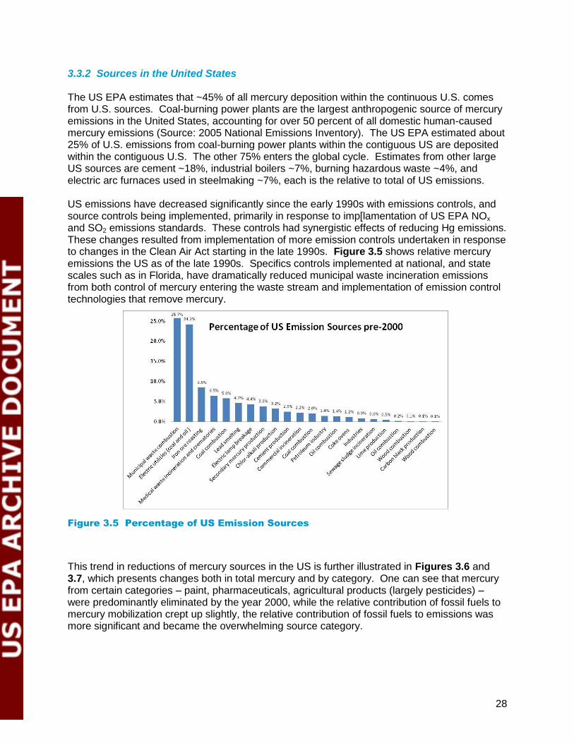
28

3.3.2 Sources in the United States The US EPA estimates that ~45% of all mercury deposition within the continuous U.S. comes from U.S. sources. Coal-burning power plants are the largest anthropogenic source of mercury emissions in the United States, accounting for over 50 percent of all domestic human-caused mercury emissions (Source: 2005 National Emissions Inventory). The US EPA estimated about 25% of U.S. emissions from coal-burning power plants within the contiguous US are deposited within the contiguous U.S. The other 75% enters the global cycle. Estimates from other large US sources are cement ~18%, industrial boilers ~7%, burning hazardous waste ~4%, and electric arc furnaces used in steelmaking ~7%, each is the relative to total of US emissions. US emissions have decreased significantly since the early 1990s with emissions controls, and source controls being implemented, primarily in response to imp[lamentation of US EPA NOx and SO2 emissions standards. These controls had synergistic effects of reducing Hg emissions. These changes resulted from implementation of more emission controls undertaken in response to changes in the Clean Air Act starting in the late 1990s. Figure 3.5 shows relative mercury emissions the US as of the late 1990s. Specifics controls implemented at national, and state scales such as in Florida, have dramatically reduced municipal waste incineration emissions from both control of mercury entering the waste stream and implementation of emission control technologies that remove mercury.

Figure 3.5 Percentage of US Emission Sources

This trend in reductions of mercury sources in the US is further illustrated in Figures 3.6 and 3.7, which presents changes both in total mercury and by category. One can see that mercury from certain categories – paint, pharmaceuticals, agricultural products (largely pesticides) – were predominantly eliminated by the year 2000, while the relative contribution of fossil fuels to mercury mobilization crept up slightly, the relative contribution of fossil fuels to emissions was more significant and became the overwhelming source category.

29

Figure 3.6 Trend of US Mercury Mobilization in Industrial/Consumer Goods and Fuels

(Source: Husar and Husar, 2002)

Figure 3.7 Trend of Estimated US Mercury Emissions to the Atmosphere (Source:

Husar and Husar, 2002)

30

Speciation of Anthropogenic Sources

Given that estimates for most coal-fired utilities are that they emit 50% to 70% of Hg as RGM and Hg (Table 3.1), local sources are an important component of the deposition in areas within 30-50 miles of these sources. This deposited RGM may be able to readily react with constituents as to begin entry into biological processes. An analysis of emissions and deposition in southern New Hampshire shows a local region of high deposition associated with local electric utility emissions (Evers, et al. 2007). In Florida, a study evaluated deposition patterns surrounding a coal power utility and evaluated local deposition patterns by tracking mercury isotopes in fuels sources and emission constituents unique to that source type (Sherman, et al. 2012).

Table 3.1 Examples of Mercury Speciation from Emission Sources

Source Particulate

Mercury (%)

Reactive Gaseous Mercury

(%)

Elemental Mercury (%)

Coal-fired electric utilities (United States)

10 40 50

Coal-fired electric utilities (Northeast) 2 68 30 Utility oil boilers 20 30 50 Municipal waste combustors 20 58 22 Medical waste incinerators 20 75 5 Pulp and paper production 20 30 50 Chlorine production 0 5 95 Hazardous waste incinerators 22 20 58 Primary and secondary metal production

10 10 80

Municipal landfills 10 10 80

USEPA 1999, Pacyna et al. 2003, NESCAUM 2005; Driscoll et al. 2007

Recent Changes in Mercury Loading

Lake sediment studies in the Northeastern United States and Europe show Hg deposition starting to increase in the late 1800s or early 1900s. This rate increases to 2.5- to 15-times pre-industrial levels by 1970s to early 1990s. (Kamman and Engstrom, 2002). Decreases in sediment Hg deposition in the Northeast, by roughly 25% have been observed in recent years, coincident with reductions in US emissions under activities such as the Acid Rain Rule. Net global emissions remained static or increased, due to increases in Asia during this same time period. It is reasonable to correlate this reduction with controls implemented in the United States on particulate matter and sulfur dioxide emissions from electric utilities that coincidentally reduced mercury emissions, and with reductions in consumer and industrial Hg use limiting post-consumer sources. The reductions realized in some emission categories are shown in Table 3.2, which shows the significant reductions realized in the Municipal Waste Combustion and Medical Waste Combustion categories between 1990 and 2005.

31

Table 3.2. Sources of Mercury Emissions in the U.S.

Industrial Category 1990 Emission tons

per year (tpy) 2005 Emission tpy Percent Reduction

Power Plant 59 53 10%

Municipal Waste Combustors

57 2 96%

Medical Waste Incinerator 51 1 98%

3.3.3 Sources in the State of Florida

Mercury sources have changed dramatically in the last 20 years, with the advent of material controls and emissions controls. The US EPA NEI 2005 emissions year (Table 3.3) shows relative loads in pounds per year and relative percentage of emission categories.

Table 3.3 2005 National Emissions Inventory (NEI) - Florida (US EPA, 2005)

Source Category

Total Mercury

Emissions

(lbs/year)

Relative Percentage of

Annual Mercury

Emissions

Coal-fired electric generation 2,094 52.7%

Cement Industry 710 17.9%

Waste-to-Energy plants 692 17.4%

Oil-fired electric generation 314 7.9%

Waste water treatment plants 102 2.6%

All others 60 1.5%

Total 3,972

Mercury, once a common constituent in batteries, has been all but eliminated from the materials and waste stream in Florida (Figure 3.8). Paints are another category in which mercury was once common, serving as an inhibitor to fungus, which has been eliminated. The overall trend of mercury sources has been on the decline in Florida (Figure 3.9).

32

Figure 3.8 Florida mercury use in electrical devices (source Husar and Husar, 2002)

Figure 3.9 Trend of anthropogenic mercury use in Florida (Source Husar and Husar,

2002)

In the last decade even Florida’s consumption of coal has been reduced because many utilities that relied on coal have constructed new faculties to take advantage of lower natural gas prices, and operated existing natural gas EGUs at higher capacity. There have been more than 10

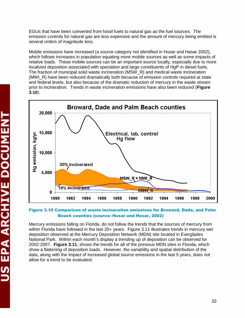
33

EGUs that have been converted from fossil fuels to natural gas as the fuel sources. The emission controls for natural gas are less expensive and the amount of mercury being emitted is several orders of magnitude less. Mobile emissions have increased (a source category not identified in Husar and Hasar 2002), which follows increases in population equating more mobile sources as well as some impacts of relative loads. These mobile sources can be an important source locally, especially due to more localized deposition associated with speciation and large constituents of HgP in diesel fuels. The fraction of municipal solid waste incineration (MSW_R) and medical waste incineration (MWI_R) have been reduced dramatically both because of emission controls required at state and federal levels, but also because of the dramatic reduction of mercury in the waste stream prior to incineration. Trends in waste incineration emissions have also been reduced (Figure 3.10).

Figure 3.10 Comparison of waste incineration emissions for Broward, Dade, and Palm

Beach counties (source: Husar and Husar, 2002)

Mercury emissions falling on Florida, do not follow the trends that the sources of mercury from within Florida have followed in the last 20+ years. Figure 3.11 illustrates trends in mercury wet deposition observed at the Mercury Deposition Network (MDN) site located in Everglades National Park. Within each month’s display a trending up of deposition can be observed for 2002-2007. Figure 3.11, shows the trends for all of the previous MDN sites in Florida, which show a flattening of deposition loads. However, the variability and spatial distribution of the data, along with the impact of increased global source emissions in the last 5 years, does not allow for a trend to be evaluated.

34

Figure 3.11 Monthly Volume-Weighted Mean Hg at Florida MDN sites

Mercury emissions from Florida sources have been in decline with the installations of emission controls on coal fired EGUs (Table 3.4). In several cases, the controls already implemented on coal-fired EGUs are achieving the mercury emission limits required by the pending MATS controls for mercury (Table 3.5) at coal-fired EGUs. The table also compares mercury emissions from 2009, a time at which only some mercury controls were fully installed and operational, with the anticipated limits under MATS being for implementation of all required controls. Also 2009 was during a significant economic slowdown when power and energy demands were reduced.

35

Table 3.4 Estimated Mercury Reduction Associated with the Mercury Air Toxic Standards Rule (MATS) (Source DARM,

2012)

Plant Name Unit ID

Capacity (MW)

On Line Year

Wet/Dry Scrubber

Scrubber Online Year

NOx Comb

Control

NOx Post-Comb

Control

SCR Online Year

SNCR Online Year

PM Control Approx. Hg Reduction

(%)

Seminole 2 658 1984 Wet

Scrubber 1984 LNBO SCR 2009 ESPC 75

Seminole 1 658 1984 Wet

Scrubber 1984 LNBO SCR 2009 ESPC 73

St. Johns River Power Park

2 626 1988 Wet

Scrubber 1988 LNB SCR 2008 ESPC 75

St. Johns River Power Park

1 626 1987 Wet


Stanton Energy Center

2 446 1996 Wet


Stanton Energy Center

1 440 1987 Wet

Scrubber 1987 LNB ESPC 57

Crystal River 1 379 1966 LNC1 ESPC 0

Crystal River 2 491 1969 LNB ESPC 0

Crystal River 4 722 1982 Wet


Crystal River 5 721 1984 Wet


Crist 7 472 1973 Wet


Crist 4 78.0 1959 2010 LNB SNCR 2006 ESPC+ESPH 76

Crist 5 78.0 1961 2010 LNB SNCR 2006 ESPC+ESPH 76

Crist 6 302 1970 Wet

Scrubber 2010 LNB+OFA SCR 2012 2006 ESPC 76

Scholz 2 49.0 1953 ESPC 0

Scholz 1 49.0 1953 ESPC 0

Lansing Smith 2 195 1967 LNC3 SNCR 2005 ESPC+ESPH 0

Lansing Smith 1 162 1965 LNB SNCR 2005 ESPC+ESPH 0

Big Bend BB03 364 1976 Wet






36

Plant Name Unit ID

Capacity (MW)

On Line Year

Wet/Dry Scrubber

Scrubber Online Year

NOx Comb

Control

NOx Post-Comb

Control

SCR Online Year

SNCR Online Year

PM Control Approx. Hg Reduction

(%)



Deerhaven Generating Station

B2 228 1981 Wet

Scrubber 2009 OFA SCR 2009 ESPC 83

Northside Generating Station

2 275 2002 Dry

Scrubber 2002 SNCR 2002 B

Northside Generating Station

1 275 2002 Dry

Scrubber 2002 SNCR 2002 B

C D. Mcintosh Jr 3 342 1982 Wet


Cedar Bay Generating LP

CBC 83.3 1994 Reagent Injection

SNCR 1994 B


CBB 83.3 1994 Reagent Injection

SNCR 1994 B


CBA 83.3 1994 Reagent Injection

SNCR 1994 B

Indiantown Cogeneration LP

AAB01

330 1995 Dry

Scrubber 1995 LNB+OFA SCR 1995 B

37 Florida Department of Environmental Protection

Table 3.5 Estimated Mercury Reduction Associated with the Mercury Air Toxic

Standards Rule (MATS) (Source DARM, 2012)

2009 emissions controls reflect EGU operations for the base atmospheric modeling year, and the projected CAMD MATS limits are the projected emission loads allowed based upon the CAMD heat inputs. Some EGUs had controls come online in 2009, which is not reflected in the 2009 loads.

Coal-fired Electric Generation Unit

Emissions with 2009 Controls

(lbs/yr)

CAMD Heat Input

(MMBtu)

CAMD MATS-limited Hg

(lbs/yr)

TECO Big Bend 106.3

Unit 1 65.5 20,504,228 24.6

Unit 2 18.7 12,866,303 15.4

Unit 3 10.9 31,424,714 37.7

Unit 4 11.2 31,965,301 38.4

LEC C.D.McIntosh 19.6

Unit 3 19.6 19,974,895 24.0

Cedar Bay Cogen 29.0

Unit A 7,058,495 8.5

Unit B 7,471,021 9.0

Unit C 6,849,345 8.2

GP Crist 327.2

Unit 4 29.0 2,448,587 2.9

Unit 5 28.5 4,135,866 5.0

Unit 6 96.4 10,635,530 12.8

Unit 7 173.3 22,037,348 26.4

PE Crystal River 528.0

Unit 1 83.0 20,859,374 25.0

Unit 2 110.0 23,734,375 28.5

Unit 4 158.0 42,114,153 50.5

Unit 5 177.0 30,288,500 36.3

GRU Deerhaven 5.3

Unit 2 5.3 14,576,952 17.5

Indiantown Cogen 19.6

Unit 1 15,651,993 18.8

GP Lansing Smith 150.1

Unit 1 70.7 5,486,938 6.6

Unit 2 79.4 9,602,261 11.5

TECO Polk Power 9.0

Unit 1 9.0 10,690,718 26.7

GP Scholz 13.6

38

Coal-fired Electric Generation Unit

Emissions with 2009 Controls

(lbs/yr)

CAMD Heat Input

(MMBtu)

CAMD MATS-limited Hg

(lbs/yr)

Unit 1 7.3 278 0.0

Unit 2 6.3 125,240 0.2

Seminole Gen. Station 54.3

Unit 1 26.3 29,206,824 35.0

Unit 2 28.0 45,703,994 54.8

JEA SJRPP/NGS 72.0

SJRPP Unit 1 29.7 39,932,826 47.9

SJRPP Unit 2 28.6 49,271,796 59.1

NGS Unit 1 8.6 18,222,684 5.5

NGS Unit 2 5.2 18,438,274 5.5

OUC Stanton 135.0

Unit 1 106.5 33,123,155 39.7

Unit 2 28.4 29,156,501 35.0

TOTALS 1469.0 717.2

Many of the above referenced units installed air pollution controls in the 2009 timeframe. 2009 emissions do not necessarily represent the full operating capacity of these units. The CAMD information is based on information submitted by the utilities to the EPA Clean Air Markets Division.

Cement production is another relatively significant source of mercury emissions (Table 3.6). This is from the combined issues of coal being used as a fuel source in the cooking of the klinker, the mercury in the limestone which is a major raw ingredient for clinker production and also that coal ash from power utilities being a common ingredient used in cement production.

Table 3.6 2009 Florida Portland Cement Production and Estimated Mercury

Emissions (source DARM, 2012)

Facility Mercury

(lb/MM ton clinker)

Mercury (Act. lb/yr)

Mercury Permitted

(lb/yr)

MACT Limit (lb/MM ton

clinker)

Mercury @ MACT (lb/yr)

American Cement

Kiln No. 1(New) 111 43 122/12-month

55 21.08

CEMEX North

Kiln No.1

No limit (~120)

55

Kiln No.2

No limit (~120)

55

TOTAL 0 0 ~240

CEMEX South

Kiln No.1 154 40 262.8 55 14.32

Kiln No.2 (New) 119 73 122 55 33.73

TOTAL

113

48.05

CEMEX Miami

Kiln No. 1 83 62 182 55 40.68

FRI

Kiln No. 1 50 23 200 55 25.31

Kiln No.2 (New) 111 24 122 55 12.05

TOTAL

48

37.36

39

Facility Mercury

(lb/MM ton clinker)

Mercury (Act. lb/yr)

Mercury Permitted

(lb/yr)

MACT Limit (lb/MM ton

clinker)

Mercury @ MACT (lb/yr)

Sumter Cement

Kiln No.1 (delayed)

184/12-month

Suwannee American

Kiln No. 1 89 53 97 55 32.55

Titan

Kiln No.1 80 78 229/12-month 55 53.52

Totals: Actual Hg: 395 MACT Limit Hg: 233.23

These source categories, the emissions inventory, were updated as part of the Florida Mercury TMDL project for the base case atmospheric modeling year of 2009. Florida emissions, by category, were derived and updated from the US EPA’s National Emissions Inventory 2005 (US EPA NEI, 2005), as presented in Table 3.7. The table shows an estimated 30% and 50% reduction in coal-fired EGU and waste-to-energy plant emissions, respectively. These reductions can be attributed to new controls and adjustments to the waste stream. The table shows a reduction of ~50% by the cement industry; however, this cannot be attributed to controls and is a result of having identified a dramatically reduced level of production in response economic conditions and the slowing of the housing market. The dramatic increase shown for Gerdau-Ameristeel is a consequence of correcting errors in the NEI 2005 for accurate information on levels of production and production methodologies at this facility.

Table 3.7 2009 Mercury Emissions Inventory in Florida (DARM & UMAQL, 2011)

Source Category 2005 NEI

(lbs/year)

Nominal 2009

DARM Update

(lbs/year)

Relative

Percentage of

Annual Mercury

Emissions 2009

Coal-fired electric generation 2,094 1,469 37.0%

Cement Industry 710 326 8.2%

Waste to energy plants 692 663 16.7%

Oil-fired electric generation 314 314 7.9%

Waste water treatment plants 102 102 2.6%

Medical waste incineration 4 2 0.1%

Gerdau-Ameristeel 13 250 6.3%

All others 43 43 1.1%

Total: 3,972 3,169

3.4 Mercury Deposition and Re-Emission

Mercury deposition can be thought of broadly as occurring under two circumstances: wet and dry deposition. As the names imply wet deposition is that which occurs in precipitation events: rain, sleet, snow, and dew. Wet deposition is measured by capturing the precipitation and securing it so that the mercury cannot evaporate or sublimate from the collection. Wet deposition is especially important in Florida because of the high frequency of convection storms (thunder storms), and the large size of these weather systems in Florida. Convection storms

40

can climb in excess of 10 miles which allows a stripping of atmospheric constituents, including mercury, from these great vertical columns, thus the wet deposition often represents the mercury in a very large volume of the atmosphere. Additionally, thunderstorms can produce winds in excess of 55 mph pulling in still more volumes of air from which the rain, or hail, strips atmospheric pollutants. Across Florida, thunderstorms are more common in inland areas by ~20%; and, across coasts to inland areas thunderstorms occur on average of 80 to 100 days per year. The scale of rain from thunderstorms often in excess of 3 inches in an hour also means that pollutants stripped from the air, and those already deposited on ground surfaces, are washed into mesic, wetland, and aquatic systems. Dry deposition as the name implies is that which occurs external to precipitation events. Dry deposition characteristics and rates are far less studied than wet deposition. This is due to the increase in complexity of capturing and measuring this form of deposition. Prior to the Department’s efforts in the mercury TMDL Project to document levels attributable to dry deposition, estimates of the relative contribution from dry deposition ranged as being 20% to being equal to wet deposition. The clear need to have accurate empirical measures for dry deposition to quantify loading of mercury deposition required state of the art science to be put in place across Florida to make dry deposition measures. Knowing only the net amount of dry deposition while being an important measure would leave so many more questions as to the nature and composition of dry deposition. The Mercury TMDL Project applied measuring methodologies that provided fine time resolution, as well as speciation of dry deposition. These provide critical data to be used toward a better understanding atmospheric chemistries and which aid in understanding mercury movement through the environment. The Department chose to measure primary atmospheric pollutants continuously such as NOx, SO2, O3, CO, as well as total mercury (THg). Mercury speciation was measured at two-hour intervals continuously. These dry deposition measures were collected at the four supersites (Pensacola, Jacksonville, Tampa, and Davie) for 14-18 months from 2009 to 2010. While rates of dry deposition varied spatially and temporally across the state, it was always close to being equal to the event driven wet deposition in terms of total mercury. The dry deposition mercury speciation and continuous measures are important in understanding the specifics and dynamics of mercury cycling within Florida. Atmospheric dry mercury is stripped by forests in leaf and needle uptake as well as in resistance knocking mercury from the air to the forest floor. Atmospheric dry mercury is taken up by prairie, shrub, and wetland plants, where this may be a critical avenue of entry into food webs, and a means of having mercury bound to organic matter enter aquatic systems. This entry into plant matter may be a primary mechanism of entering biological systems and food webs. Based upon the literature, estimates of a mean volatilization rate of Hg0 from soil is roughly 11 pg per square-meter per hour. This rate would reemit most of the atmospheric Hg0 deposition onto bare soils or hard surfaces. However, the uncertainty of this process identifies an area for additional research on Hg re-emissions. This re-emission cycle would be especially important in areas which can subsequently have deposition enter ecological systems, such as areas with significant cover of wetlands or forests, and with high levels of rainfall and daily dew deposition.

3.5 Mercury Movement in the Environment

Before we get into the detailed discussion of mercury transport in different ecosystems, we can use a general summary here to describe the major pools of mercury in natural systems and the dynamics of mercury among these pools (see Figure 2.1).

41

Some studies looking at the environmental fate of mercury showed high THg and MeHg concentrations locations far from identified point source emissions. What has uniformly been identified as locations where mercury is accumulating in the environment is low lying, flat areas (wetter systems, e.g., mesic and wetland systems) (Dennis et al., 2005); those areas where precipitation accumulates in landscapes. Also Total Organic Carbon (TOC) correlated well with THg and MeHg. For Florida this indicates much of the environment – flat, wet, high in mesic forest and wetland cover – is very suitable in almost all areas of the state and such cover is close to emission sources. In Washington State, a study looked at sediment profiles in three lakes of varying distance from the emission source a coal fired power plant, and found mercury profiles in sediments reflecting the emissions history of the regional source, by load and distance (Furl et al. 2011). Mercury risks to human health, or wildlife, require exposure that occurs primarily, though not exclusively, through fish consumption. The amount of mercury that is methylated in ecosystems is only a very small fraction of the mercury that is deposited in ecosystems. Sources that deposit mercury into ecosystems, whether from emissions or direct discharge, natural or anthropogenic, are the means by which mercury becomes available to be transformed into toxic methylmercury within the ecosystems and then bioaccumulated up food chains into fish.

3.5.1 Mercury transport and fate in forest ecosystems

Studies of direct soil sequestration of Hg, immobilization of Hg in forest soil, show a correlation with the retention of organic carbon (Schwiseg, 1999). Pools of Hg in upland soils in northern temperate regions are about 7 mg per m2, with higher levels reported around the globe, so this is only a reference number. The export of Hg by waters draining upland soils to surface waters is generally low. Concentrations and fluxes of Hg in soil waters, analogously to the pattern in soil, are closely related to dissolved organic carbon content. Concentrations of total Hg are highest in waters draining the upper soil, coinciding with high concentrations of DOC. The conditions optimal for this occurrence are shallow, flat systems with wet high organic soils as is predominant in Florida. Concentrations and fluxes of total Hg decrease as DOC is immobilized with depth in mineral soil (Grigal, 2002). Limited studies suggest that MeHg concentrations in upland soils and ground waters are generally low, although higher concentrations occur in upper soil waters and decrease with soil depth. Low concentrations and fluxes of MeHg in drainage waters suggest that rates of methylation are low, and freely draining upland soils are generally not important in the supply of MeHg to downstream surface waters, with the possible exception of recently harvested forests (Porvari et al., 2003).

3.5.2 Mercury in Wetlands: transport and transformation

Wetlands influence the composition and supply of different Hg species to adjacent surface waters. Wetlands are typically net sinks of total Hg and sources of MeHg (Grigal 2002). Rates of total Hg accumulation are greater in wetlands than in upland soils because of the strong association of Hg with organic matter (Grigal, 2003). Annual rates of MeHg production in wetlands are approximately 0.1 to 1 µg per m2 per year (Galloway and Branfiruen, 2004). The factors controlling methylation of Hg in wetlands are not completely understood, but they most likely involve the amounts and types of organic matter, water and soils chemistries, hydrologic flow paths, microbial composition, microbial locations relative to flow paths, and rates of microbial activity, as well as any limiting resource for microbial activity. Organic matter produced in wetlands forms complexes with both ionic Hg and MeHg, enhancing the transport of

42

these Hg species to surface waters. There is debate on how these complexes in some cases enhance later consumption by single celled organisms or are perhaps incidental in consumption by first level secondary consumers. An elevated supply of DOC to downstream surface waters may stimulate conditions for mercury methylation, and limit mercury available for photodegradation and photoreduction of HgII. Concentrations of MeHg in wetland pore waters and surface waters vary seasonally, with the highest concentrations evident during the late summer, as a result of warmer temperatures, higher rates of microbial activity, and longer hydraulic residence times (Galloway and Branfireun 2004).

3.5.3 Mercury in surface waters

Freshwater ecosystems vary in how they respond to Hg pollution. Total Hg concentrations in surface waters in the Northeast vary by more than an order of magnitude across systems, from less than 0.5 to 12.7 nanograms per liter, the 5th to 95th percentile respectively (Dennis et al., 2005). Most of the Hg in surface water occurs as HgII, with MeHg ranging from 1% to 35% of total Hg. Under conditions of high total Hg loading, MeHg production can vary widely, depending on the methylation efficiency of a particular ecosystem. Other factors controlling mercury in surface waters Other factors, such as water chemistry, land cover and land use, and watershed disturbances, alter the transport, transformation, and bioavailability of Hg in surface waters. Acidic deposition and the associated sulfur alter the acid-base status of surface waters, thus influencing Hg transformation potentials, may influence Hg uptake by sulfur reducing bacteria (SRB), and associated bioaccumulation in fish. Sulfur chemicals are closely coupled with Hg dynamics. The solubility of Hg increases with sulfide concentrations in anoxic waters through complexation reactions, potentially increasing the pool of Hg available for methylation (Benoit et al., 2005). The relationship of mercury to acidification is also related as the required controls under Acid Rain Rules promulgated under the Clean Air Act serve to control SO2 and NOx emissions which directly cause acid rain which brings about surface water and soil acidification. Watersheds with mixed agriculture and forest land cover had the highest methylation efficiency, even where these watersheds had low total Hg in sediments. Waters draining agricultural landscapes have relatively high concentrations of total Hg and MeHg due to mercury binding to organic particulates and higher methylation rates. These can also have lower concentrations in fish, due to algal "bloom dilution" associated with high phosphorus loading or elevated DOC concentrations (which stimulate methylation but limit bioaccumulation), or both (Kamann et al., 2004). Forest harvesting has been shown to increase export of total Hg and MeHg (Porvari et al., 2003). Fire results in a complex pattern of Hg loss from watersheds. During and shortly after fire, elevated Hg losses are associated with volatilization from soils and losses from erosion, as well as increased pore water flushing (Grigal 2002). It is important to remember that while forest harvesting increases turnovers and scales by anthropogenic actions, that human initiated forest fires are reflecting natural fire ecology. Thus, forest harvesting can expose soils increasing aspects of the mercury cycle, managed fires are merely mimicking natural fire ecology and not increasing mercury loads. Deforestation efforts, especially areas without a natural fire ecology, as seen in the developing world, are a source of mercury through both the burning of above ground biomass and through the exposure, including associated tilling, of soils which readily volatilize any associated mercury. Activities that manage water levels create significant exposure-saturation patterns, especially systems such as reservoirs or soil management programs as with rice, soybeans, or sugar cane, can be sources of increased

43

mercury emissions and increased pulses of MeHg formation. These often located in floodplains and converted wetland systems, provide areas of mercury binding to organic matter enhanced by soil management associated with planting and prime environments for methylation. In reservoir systems the littoral zone can fluctuate wetting and drying, thereby varying natural cycles of reduction and oxidation both by location and extent, enhancing the production of MeHg (Evers et al., 2007; Sorensen et al., 2005). Habitat type also has an important influence on MeHg concentrations. Data for two-lined salamanders (Eurycea bislineata) identified in headwater streams have significantly higher MeHg concentrations than those in lakes (Bank et al., 2005). Larval insects in reservoirs have been shown to have THg concentrations that are 3 to 10 times higher than those in natural lakes (Tremblay et al. 1996). Crayfish (Orconectes virilis) in headwater streams have THg concentrations up to five times greater than those in lakes (Pennuto et al., 2005). The landscape position of each of these may explain the differences observed. Forested regions, where wetlands are prevalent, and with low productivity surface waters, promote high concentrations of mercury in freshwater biota and thus are particularly sensitive to mercury deposition.

3.5.4 Mercury moving through organisms

Biota are exposed to MeHg primarily through the roles played by bacteria, and fish and insect consumption. The Northeastern Ecosystem Research Cooperative (NERC) data establish robust Hg exposure profiles for fish, birds, and mammals and highlight the importance of habitat type, foraging guild, trophic structure, and demographics on MeHg exposure (Evers et al., 2005). In general, THg concentrations vary by species taxonomy. As a general rule, MeHg increases with increasing trophic position. Mercury in benthic invertebrates and larval insects has been studied in northeastern lakes and reservoirs, where it was observed that even in invertebrates, increased mercury per biomass is associated with an increase in trophic level (odonates > hemipterans / coleopterans > trichopterans > dipterans / ephemeropterans) (Tremblay et al., 1996). The NERC data on Hg in over 15,000 fish show that the mean fillet THg levels in 10 of the 13 species are above EPA guideline of 0.3 µg/g and highest in top level predators such as walleye (Sander vitreus) and lake trout (Salvelinus namaycush).

44

Chapter 4: TMDL Approach

4.1 General Approach

To address the mercury impairment in Florida waters, the Department selected a statewide6 approach for mercury TMDL development, rather than a waterbody-specific TMDL approach for the following reasons. First, the predominant source of mercury leading to impaired waters in Florida is from atmospheric deposition. The majority of atmospheric mercury deposited on Florida, >95%, as well as the emission sources, comes from outside of Florida. Mercury in the atmosphere is transported across multiple watershed boundaries, where it is deposited and biologically magnified through the food web, resulting in high fish tissue concentrations. While a watershed-based TMDL approach is typical for most pollutants, the phenomenon of atmospheric transport of mercury makes a regional or statewide approach the only practical method for TMDL development. This approach is consistent with other mercury TMDL efforts supported by US EPA, including multi-state efforts. EPA recognized the sources of the mercury impairments were largely from outside the borders of individual states and issued a guidance document (USEPA, 2008), which supported the concept of addressing the problem at scales ranging from waterbody-specific, regional, statewide, or multi-state.

Second, the statewide approach will be far more cost-effective than the waterbody oriented approach. Using the IWR listing process, the Department has verified the mercury fish tissue impairment in more than 1100 water segments, as shown in Table 1.2. Rather than attempting to develop a mercury TMDL for each of these waterbodies, the proposed approach will focus on reducing mercury emissions statewide to benefit all Florida waterbodies, especially those susceptible to mercury bio-magnification (e.g., oligotrophic, low alkalinity systems). Although the concept of conducting this type of regional TMDL analysis is relatively novel, a similar predicate was established as part of the 1990 National Acid Precipitation Assessment Program Integrated Assessment. For that program, EPA conducted regional simulations for thousands of lakes in the Upper Midwest, the Adirondacks, and Florida to evaluate how lakes would behave in response to Clean Air Act mandated changes in sulfate emissions, which in turn were predicted to reduce acidic deposition.

Key elements that a mercury TMDL should consider were recommended by EPA (USEPA, 2008). These elements include:

(1) Identification of waterbodies, pollutant sources (2) Water quality standards and TMDL target (3) Loading capacity – Linking water quality and pollutant sources (including point and

nonpoint sources) (4) Conducting load and wasteload allocations to nonpoint and point sources (5) Establishing a margin of safety of the TMDL to address the uncertainties associated with

the target development.

6 To the extent that this draft reads as though it applies to more than the WBIDs in Appendix A, this proposal only applies to the WBIDs in WBID A.

45

A technical framework was established by the Department to address the TMDL needs listed above (Figure 4.1). A sampling protocol was designed to measure fish tissue mercury concentrations, concentrations of total mercury, MeHg, and other biogeochemical parameters (for both water column and sediment from lakes) that may influence the mercury dynamics in Florida waters were collected in numerous Florida streams (129) and lakes (130) that were chosen based on a stratified statistical sampling design. Historic data, including fish tissue mercury concentration data collected through the fish consumption advisory program jointly carried out by the Department of Health (DOH), Florida Fish and Wildlife Conservation Commission (FFWCC), and the Department, water chemistry data collected through Department’s Integrated Water Resource Monitoring Network (IWRM) were also examined to identify the historic trend of mercury impairment in the State of Florida. These data and fish consumption data collected through the largest consumption study to date, were used to establish the TMDL for mercury.

In addition, to aid with subsequent evaluations of the impacts to Florida’s waters, from sources both within and outside Florida, the Department developed a technical framework designed to quantify and assess the sources and impacts of mercury from atmospheric deposition. Technical components included quantifying mercury loadings into Florida and identifying the contribution from local sources, regional sources, United States sources, and sources in other countries. In order to quantify the mercury loading into the state, predictive atmospheric models were used to simulate mercury loadings from different sources and quantify the atmospheric deposition flux. Air monitoring networks were also established to measure wet and dry depositions at several strategic locations across the State to provide measurements for model evaluation, to characterize seasonal dynamics of the air deposition, and to examine the spatial effects of major emission centers in the states. Site monitoring locations were specifically established within regions of known point source emissions, which differs significantly from MDN locations which are deliberately located away from known emission sources. This allows identification of local conditions, but also creates monitoring requirements of capturing a more variable system. The TMDL approach of assigning percent reduction to sources, has each respective mercury source be responsible only to their loading, i.e., no source is more weighted for reductions than another.

46

Figure 4.1 Overview of Technical Components of a Mercury TMDL Project

47

4.2 Mercury Atmospheric Deposition Monitoring

The Department contracted with the University of Michigan to conduct extensive seasonal field sampling activities regionally around four continuous sampling sites in Florida (Pensacola, Jacksonville, Tampa, and Davie) in the period 2008-2010. The atmospheric sampling sites were established to be able to collect wet and dry deposition data. Details of these efforts are contained in Appendix F.

Table 4.1 Initiation & End Dates of Supersite and Wet Only Site Data Collections

Air & Dry Deposition Wet Deposition

Site Start End Start End

Davie 4/3/2009 8/31/2010 2/2/2009 8/29/2010

Tampa 1/12/2009 8/31/2009 1/29/2009 8/24/2010

Jacksonville 3/9/2009 8/30/2010 3/18/2009 8/29/2010

Pensacola 10/1/2008 8/31/2010 10/7/2008 8/29/2010

Orlando 3/21/2009 8/2/2010

ENP 11/30/2008 8/30/2010

4.3 Mercury Atmospheric Modeling

The Department also contracted with the University of Michigan to perform atmospheric modeling through scaled analyses starting at a global scale with an 80 km grid and concluding at a 4 km grid scale for Florida. The details of this effort are described in Appendix F.

4.4 Mercury Aquatic Cycle Modeling

The Department also contracted with ALL to perform inferential aquatic modeling, a statistical assessment applying partition analyses for the lakes (more than 7,700 lakes greater than 4 ha in size) and stream/river reaches (more than 83,400 km of stream and riverine reaches) within Florida (see Appendix L).

4.5 Sampling of Fish Tissue and Collection of Chemical and Biochemical Data from the Water Column and Sediment

Developing Mercury Aquatic Models is an essential part of the Mercury TMDL development for impaired Florida waters. The goal of the modeling is to establish a functional relationship between the mercury loading into receiving waters and the fish tissue mercury concentration in these waterbodies. Past studies have demonstrated that, while fish tissue mercury concentration for each individual receiving waterbody may show a linear response to the change of mercury loading into the waterbody, the fish tissue mercury concentrations across lakes and streams were dominated by biogeochemical and landscape variables other than mercury loadings (Riva-Murray et al., 2011; Liu et al., 2009; Kamman et al., 2005; Selvendiran et al., 2008). Therefore, collecting water quality and sediment samples in tandem with the collection of fish tissue mercury concentration is required in order to develop aquatic models. These needed fish data were collected and analyzed by the Florida Fish and Wildlife

48

Conservation Commission (FWCC) and the Department jointly through a monitoring program conducted in a period from September of 2008 through October of 2010. In order to ensure a sufficiently broad data range and reasonably even distribution of data across the gradient of each sampled parameter for statistical analyses, sampling sites for needed parameters were chosen using a stratified random sampling design. Basically, the concentration ranges of three target variables (pH, color, and chlorophyll a for lakes; pH, color, and nitrate for streams) from lakes and streams included in the Department’s Status Monitoring Network (SMN) were examined. The identified concentration ranges of these parameters were divided into 5 concentration intervals for each parameter, which yielded a possible 125 unique variable interval combinations (5x5x5) or sampling bins. The actual numbers of bins that were populated by at least one lake or stream reach were 101 and 95, respectively. Additional lakes and streams were sampled at random from individual bins to produce a total number of 133 lakes and 131 streams segments for the sampling. For each selected waterbody, 12 large-mouth bass (LMB) were collected for total mercury analyses. LMB were selected as representing a top level predator in systems in which they are present, thus having the greatest rates of bioaccumulation. Size of sample fish was determined by the current (FY08/09) FFWC’s size regulations for black bass; however, LMB up to 2” less than the minimum size regulation up to approximately 20” were collected in order to establish robust relationship between fish tissue concentration and fish size. Where it was infeasible to collect 12 LMB, spotted sunfish (SPSU) were collected across a range of available sizes. Preliminary analyses comparing concurrently collected LMB and SPSU indicated well-correlated tissue mercury concentrations between these two fish species. These sample fish were collected by FWCC and shipped to Eustis Fisheries Research Laboratory, or other FWCC facilities for tissue sample preparation. Prepared fish tissues samples were transported to Department’s Central Laboratory for total mercury analyses. Other than fish sample collection, FWCC also collected concurrent water quality samples from the same lakes and streams where fish samples were collected. Water quality samples were collected for measurement of aqueous mercury species and ancillary water quality parameters including major ion, dissolved organic carbon (DOC), color, total suspended solid (TSS), and nutrients. Field measurements, including dissolved oxygen, conductivity, and Secchi depth, were also collected. Water quality samples collected by the FFWC were shipped via overnight courier to Department’s Central Laboratory in Tallahassee for analyses. In order to provide a complete dataset to describe factors that influence the mercury fish tissue concentrations in Florida waters, sediment sample were also collected in lakes where fish and water quality samples were collected. Lake sediment sample collections were conducted by the Department and were in parallel to the sample fish and water quality sample collection efforts made by FWCC. Sediment sample analyses were conducted by Department’s Central Laboratory. These analyses focused on mercury and MeHg, metals (aluminum, arsenic, cadmium, cobalt, chromium, copper, iron, potassium, magnesium, manganese, nickel, lead, antimony, selenium, strontium, titanium, vanadium, and zinc and nutrients. All sample collections were conducted in the period from September of 2008 through October of 2010. Sample collections were conducted once for each selected waterbodies. Figure 4.2 shows the location of sampling sites. Results from sample analyses were summarized in Chapter 5 of this report. All field and laboratory procedures for collection of fish samples adhere to the guidelines established in the Comprehensive Quality Assurance Plans for Collection of Fish established for FWCC (FWC Chemistry Laboratory SOP, HGSOP 4/03) and FDEP (DEP-

49

SOP-001/01, FS6000 General Biological Tissue Sampling). All field and laboratory procedure for collection and analysis of water samples and laboratory analysis of fish tissue samples were adhere to the requirements set forth in Department’s Quality Assurance Rule, Chapter 62-160, F.A.C), including Department’s Standard Operating Procedure (SOPs) for field activities (DEP-SOP-001/01).

50

Figure 4.2 Mercury TMDL Project Sampling Sites

4.6 Historic Data for Fish Tissue Mercury Concentration and Water Column Chemistry

51

Other than the fish tissue, water column, and sediment data collected during the 2008-2010 monitoring program, historical data collected through the fish consumption advisory program jointly carried out by the Department, FFWC, and DOH, and by the Department’s Integrated Water Resource Monitoring Network (IWRMN) were also examined in order to identify the temporal trend of mercury fish tissue impairment in Florida. Since 1983, FWCC, DOH, and the Department have been jointly conducting investigations on fish tissue mercury impairment in Florida waters. This effort primarily focuses on waterbodies and fish species that are important for fishing activities. Samples of popular fish species, such as LMB, bluegill, redear, sunfish, warmouth, spotted sunfish redbreast sunfish, black crappie, catfish, some exotics such as Oscars, butterfly peacocks, and Mayan cichlids, and over 100 salt water species such as Atlantic croaker, black grouper, dolphin, fantail mullet, gray snapper, gulf flounder, king mackerel, spotted seatrout, and yellowfin tuna, have been collected by FWCC from freshwater and marine waterbodies identified by FWCC and shipped to the Department for tissue mercury analysis. Fish consumption advisories for specific water bodies are issued by DOH if the mercury concentration found in fish is at levels that may pose a risk to human health. Advisories for mercury in Florida waters have been issued since 1989. The DOH Web site (www.doh.state.fl.us/floridafishadvice) offers regularly updated consumption advisories containing specific advice about eating fish from Florida's fresh and marine waters. These advisories are not intended to discourage fish eating but to provide guidance for choosing the right fish and also limit eating fish from waterbodies of high concern of mercury pollution. For the mercury TMDL, the Department obtained fish tissue results of over 30,000 fish samples collected from more than 300 freshwater segments. Result summarizations of these data are provided in Chapter 5 of this report.

As mercury fish tissue concentrations can be influenced both by external mercury loadings into the aquatic system and biogeochemical characteristics of receiving waters, it is desirable to pair the analyses on mercury fish tissue concentration data with the analysis of water quality data. The water quality data used in these analyses were primarily retrieved from Department’s IWR Database, which included data collected by Florida’s Integrated Water Resource Monitoring Network (IWRM, http://www.dep.state.fl.us/water/monitoring/index.htm). This network was initiated in 1996 by the Department in an effort to refining its water resource monitoring and included three tiers of monitoring programs. Tier I monitoring program include status monitoring and trend monitoring. These monitoring networks primarily focus on providing the spatial and temporal water quality trend in Florida at the state level. Tier II monitoring program is watershed and waterbody oriented. It includes not only the monitoring efforts of the Department on individual waterbodies, but also collects water quality monitoring results from more than 90 other entities including other state agencies, county and local governments, universities, and voluntary groups. Water quality results from the Tier II monitoring program constitute the vast majority of the water quality data that the Department uses to conduct the IWR listing process and develop TMDLs for impaired waters. Tier III monitoring are primarily associated with the monitor activities required through the Department’s regulatory permits, which is used to evaluate the effectiveness of point source discharge reductions and implementation of best management practices required by TMDLs.

http://www.doh.state.fl.us/floridafishadvice

http://www.dep.state.fl.us/water/monitoring/index.htm

52

0

0.1

0.2

0.3

0.4

0.5

0.6

0.7

0.8

0.9

1

0.000 0.200 0.400 0.600 0.800 1.000 1.200 1.400 1.600

Pe

rce

nti

le D

istr

ibu

tio

n

Fish Tissue Mercury Concentration (mg/Kg)

Lakes Streams

Chapter 5: Monitoring Results

5.1 Fish Tissue Results

Fish tissue data were collected from 133 lakes and 131 streams in Florida in the period from September 2008 through October 2010. The fish tissue sampling focused on LMB; however, for those waterbodies in which no LMB could be collected or not enough LMB could be collected, spotted sunfish (SPSU) or spotted bass (SPB) were collected in place of LMB, using a translation between species to a common normalized fish standard. Out of the total 264 waterbodies sampled, fish samples from 90 waterbodies included SPSU samples and from 7 waterbodies included (SPB samples). Average fish tissue concentrations were calculated for each species in each waterbody and median values of these waterbody-species average were then determined. The median tissue mercury concentration for LMB, SPSU, and SPB, based on fish samples collected in this project were 0.40 mg/Kg, 0.25 mg/Kg, and 0.68 mg/Kg, respectively. The 90th percentile fish mercury concentrations for LMB, SPSU, and SPB were 0.89 mg/Kg, 0.43mg/Kg, and 1.02 mg/Kg, respectively. Figure 5.1 shows the distribution of fish tissue mercury concentration based on data collected from the above sampling project after the fish tissue normalization was conducted. Detailed information regarding the location of sampled waterbodies, general sampling conditions, and water chemistry of the sampled waterbodies can be found in Appendix H of this report.

Figure 5.1 Cumulative Frequency of Fish Tissue Mercury Concentration in Lakes and

Streams.

Fish tissue concentrations were also collected through the Florida fish consumption advisory program jointly carried out by FWC, DOH, and the Department since 1983. Based on the LMB data collected through the program, there appear to be a general trend of decrease in fish tissue concentration since the early 1980s (Figure 5.2), although the probability that the slope of the decreasing line is zero is slightly higher than the 0.05 level .

53

Figure 5.2 Dynamics of Fish Tissue Mercury Concentration in Florida Waters in the

Period from 1983 through 2011

5.2 Total and Methylmercury, and other Water Column Parameters

Water column samples were collected from the same waterbodies and at the same time when fish samples were collected and sent to the Department’s Central Lab for analysis. These data include total mercury, MeHg, and other water quality parameters. Figures 5.3a and 5.3b show the accumulative distributions of total mercury and MeHg in lakes and streams, respectively.

Figure 5.3a Cumulative Frequency of Total Hg and Methyl-Hg Water Column

Concentrations in Lakes

y = -0.0069x + 14.258 R² = 0.1479

0

0.1

0.2

0.3

0.4

0.5

0.6

0.7

0.8

0.9

1

1980 1985 1990 1995 2000 2005 2010 2015

Fish

Tis

sue

Tota

l Mer

cury

Co

nce

ntr

atio

n (

mg/

Kg)

Year

0%

10%

20%

30%

40%

50%

60%

70%

80%

90%

100%

0.00 1.00 2.00 3.00 4.00 5.00 6.00 7.00 8.00

Dis

trib

uti

on

Pe

rce

nti

le

Concentration (ng/L)

Total Hg Methyl-Hg

54

0%

10%

20%

30%

40%

50%

60%

70%

80%

90%

100%

0% 10% 20% 30% 40% 50% 60% 70% 80% 90%

Dis

trib

uti

on

Pe

rce

nti

le

Percent Methyl-Hg in Total Hg

Lake Stream

Figure 5.3b Cumulative Frequency of Total Hg and Methyl-Hg Water Column

Concentrations in Streams

The ranges of total mercury concentration in lakes and streams were fairly similar. The total mercury concentration in sampled lakes ranged from 0.22 to 7.70 ng/L. In streams, the range was 0.10 to 7.90 ng/L. However, stream total mercury concentration tended to distribute more toward the higher concentration end than the total mercury concentration in lakes. Based on Figure 5.3a, the 50th percentile of the lake total mercury concentration was 1.30 ng/L, which means that the total mercury concentration in about 50% of the lake was higher than 1.30 ng/L. In contrast, in more than 63% of the stream segments being sampled, the total mercury concentration was higher than 1.30 ng/L(Figure 5.3b). A similar trend was also observed with MeHg. The 50th percentile of the MeHg concentration in lakes was about 0.08 ng/L, which means that the methyl-mercury concentration is higher than 0.08 ng/L in about 50% of the lakes. For streams, more than 78% of the stream segments being sample had MeHg concentration higher than 0.08 ng/L. To examine the methylation potential in streams and lakes, a ratio between MeHg and total mercury was calculated for each waterbody sampled, and the accumulative frequencies of the ratio were presented in Figure 5.4 for both lakes and streams. Again, the overall distribution shows that, in stream segments, the ratio between MeHg and total mercury concentration tended to be higher than in lake segments. While the 50th percentile of the lake methyl to total mercury ratio was about 7%, the ratio of stream segments at the same percentile was about 12%. Except for one point at about the 99 percentile, the entire accumulative frequency curve of the stream methyl to total mercury ratio lain to the right of the lake methyl to total mercury ratio, indicating higher methyl to total mercury ratio in most stream segments sampled than in lakes.

0%

10%

20%

30%

40%

50%

60%

70%

80%

90%

100%

0.00 1.00 2.00 3.00 4.00 5.00 6.00 7.00 8.00

Dis

trib

uti

on

Pe

rce

nti

le

Concentration (ng/L)

Total Hg Methyl-Hg

55

Figure 5.4 Cumulative Frequency Curve for the Methyl to Total Mercury Water

Column Ratio in Lakes and Streams

Spatial distribution of total mercury, MeHg, and methyl-to-total mercury ratio in lakes and streams across the State were also examined. Detailed spatial distributions of these parameters can be found in Appendix I. Basically, no clear explicit spatial distribution patterns were identified from these analyses. Statistics of other water parameters were summarized in Table 5.1. The raw data used to calculate these statistics can be found in Appendix H.

Table 5.1 Mean and Standard Deviations for all Parameters Measured or Collected in

Waters Sampled for the Mercury TMDL

- = Sediment data were only collected for lake sampling locations

Lakes Streams

Parameter Mean Standard Deviation Mean Standard Deviation

Alkalinity (mg/L) 37.50 44.58 90.13 80.89

Field Measurements

Sample Depth 0.89 0.27 0.76 0.28

Secchi Depth 1.35 0.92 1.15 0.74

Site Depth 3.46 2.19 1.96 1.48

DO (mg/L) 7.52 2.10 5.88 2.48

pH 7.03 1.37 6.74 1.15

Specific Conductance (µmhos/cm) 307.04 733.83 487.32 1185.85

Temperature (⁰C) 23.41 6.40 21.90 4.56

Redox (mvolt) 247.81 133.75 250.34 137.83

Major Ions

Calcium (mg/L) 19.14 21.22 40.17 35.19

Chloride (mg/L) 58.81 215.07 79.48 336.51

Magnesium (mg/L) 7.02 15.57 10.79 27.15

Potassium (mg/L) 3.99 5.72 3.32 7.80

Sodium (mg/L) 32.48 120.72 49.53 215.91

56

0%

10%

20%

30%

40%

50%

60%

70%

80%

90%

100%

0 0.05 0.1 0.15 0.2 0.25 0.3 0.35 0.4 0.45 0.5

Pe

rce

nti

le D

istr

ibu

tio

n

Sediment Mercury Concentration

Total Hg Methyl-Hg

0%

10%

20%

30%

40%

50%

60%

70%

80%

90%

100%

0.00% 5.00% 10.00% 15.00% 20.00% 25.00%

Pe

rce

nti

le D

istr

ibu

tio

n

Sediment Methyl to Total Mercury Ratio

Lakes Streams

Parameter Mean Standard Deviation Mean Standard Deviation

Sulfate (mg/L) 25.03 47.12 29.07 55.74

Trophic Status Parameters

Carbon- Organic (mg/L) 13.43 10.09 16.57 14.65

Ammonia (N) (mg/L) 0.06 0.21 0.04 0.05

Nitrogen- Total Kjeldahl (mg/L) 1.23 0.90 0.85 0.57

NNOx (mg/L) 0.05 0.13 0.26 0.45

Phosphorus- Total (mg/L) 0.06 0.09 0.12 0.20

Chlorophyll a (ug/L) 18.78 36.33 4.32 11.54

Chlorophyll a- uncorrected (ug/L) 20.87 39.31 5.15 13.67

Pheophytin (ug/L) 2.61 5.64 1.28 3.40

Water Clarity Parameters

Color (PCU) 90.49 111.92 147.27 149.84

TSS (mg/L) 7.83 10.89 6.12 4.79

5.3 Sediment Mercury

Sediment total mercury, MeHg, and other sediment parameters were also collected for the 133 lakes. Figure 5.5 shows the accumulative frequencies of sediment total and MeHg concentrations. Figure 5.6 shows the accumulative frequency of sediment methyl to total mercury ratio.

Figure 5.5 Cumulative Frequency of Sediment Total and MeHg Concentration

57

Figure 5.6 Cumulative Frequency of Sediment Methyl to Total Mercury Ratio

Compared to the water column methyl-to-total mercury ratio, which mostly fell in the range from 1% to 40%, the sediment methyl to total mercury ratio was significantly lower. It mostly fell in the range from 0.02% to 5%. Statistics of other sediment parameters were summarized in Table 5.2. The raw data used to calculate these statistics can be found in Appendix H.

Table 5.2 Statistics Summary of Other Sediment Parameters (mg/kg)

Parameter Mean Standard Deviation

Al 19126.79 20204.63

Cr 28.28 27.34

Fe 8489.10 9354.47

Mg 1898.84 2453.72

Mn 82.37 103.47

Ni 9.78 8.52

K 1361.12 1559.38

Sr 158.88 280.10

Ti 1859.05 1622.37

V 28.35 27.64

Zn 51.58 118.80

Sb 0.99 3.54

As 4.41 3.59

Cd 0.52 0.55

Cu 78.40 651.48

Pb 26.96 22.87

Se 2.24 1.78

Org C 16.30 15.66

Tot C 17.13 15.43

TKN 11587.91 11330.35

TP 1284.14 1684.14

58

Chapter 6. Model Results

6.1 Summary of Atmospheric Modeling Results

The deterministic atmospheric modeling performed as part of the Mercury TMDL Project analyzed various scales from global (80km resolution) to Florida region (4km resolution). The resolution of the modeling became more finite as the models scaled down to Florida. The model scales went from an 80km grid for the global domain, to 56 km for the North American domain, to 12 km for the Southeastern US domain, to a 4km domain for Florida. This 4km domain is the most resolute statewide modeling performed to date by any entity world-wide. As part of the development of the deterministic atmospheric model, meteorological models at the same domains had to be developed to handle the transport of atmospheric constituents. To provide load inputs into each scale of the model emissions inventories were developed with increasing specificity such that for Florida all individual major emission sources were specifically updated to current controls and operating levels for the 2009 base model year. The deterministic atmospheric chemistry modeling, meteorological modeling, and emissions processing were all performed through publically available, public domain, models (see Appendix F). These models were enhanced through resolution of bug fixes, discovered when applying the models at the varying scales, as well as coding. All bug fixes were documented in the revised coding as well as being posted to the information boards publically maintained by the respective agencies managing this public domain software (this coding has been supplied to entities that have requested it, such as groups representing coal fired power industry in Florida). All enhancements were posted to the website for the models, and included in subsequent versioning. One pioneering enhancement in this effort was the implementation of a tagging scheme by which emission source categories could be tracked as to identify the source of deposition onto Florida. The source categories tracked in the atmospheric model are:

Florida electric coal fueled Florida electric oil fueled Florida waste-to-energy Florida other sources grouped Alabama sources Georgia sources Mississippi sources Louisiana sources Texas sources Other US sources Global sources coming into USA Deposition re-emission

Another modeling effort is referred to as Inferential Dry Deposition Modeling. This allows an extrapolation of measured monitoring data to Florida statewide. This effort looks at conditions of land cover, such as forests or urbanized areas, meteorology, and their affects on how mercury gets deposited onto land surfaces. This enhances estimates of dry deposition. A third atmospheric modeling effort examines the source types that are depositing at the atmospheric monitoring locations. This effort uses two different public domain statistical analysis packages to identify chemical constituents in atmospheric deposition that best explain the variation in the deposition measured. These models are EPA’s PMF (USEPA, 2007) and Unmix (USEPA, 2007). Each of these through different algorithms, and PMF allowing the added use of uncertainty, perform partition analyses that use the full suite of constituents measured. The partition analyses provide arrays of constituent combinations that best represent the variability in constituents measured. Based upon the mix of constituents, and their relative amounts in a given array one can relate these to established profiles of source emissions. For additional information and results please see Appendix F.

6.2 Overview Inferential Aquatic Modeling

The inferential aquatic modeling performed as part of the Mercury TMDL project sought to identify rigorous relationships between fish tissue THg, water quality measures, sediment quality measures, and modeled atmospheric deposition. These assessments were made through a wide range of statistical analyses applying parametric and nonparametric approaches, graph analyses, neural network analyses, fuzzy logic, and partition analyses. The data sets used were those collected for the 133 lakes and 131 streams, as well as expanding this data set with an additional 100 measures from historic fish tissue and water quality measures that were collected. The expanded fish tissue data were supplied by Ted Lange of FWC, and the water quality data were pulled from the SMN data. The added data were selected because near coincidence in time of fish tissue and water quality measures and these being in close time frame to the data collected as part of Mercury TMDL Project. For additional information and results please see Appendix L.

60

Chapter 7: TMDL Target Setting

7.1 Setting a Reduction Target Based on Mercury in Fish Tissue

7.1.1 Reduction Target for Fish Consumption by Humans

In Florida, waters are identified as impaired based upon The Florida Department of Health (FDoH) fish consumption advisories that evaluate mercury concentrations in fish tissue (62-303.470). FDoH is the lead state agency for providing fish consumption advisories, which are published periodically to alert Floridians about possible contamination issues linked to fish caught in Florida’s waters. A series of “Quick Facts” and the advisories can be viewed at: http://www.myfloridaeh.com/medicine/fishconsumptionadvisories/index.html. FDoH provides general and specific guidelines that discuss the benefits and risks of eating fresh water and marine fish species, balancing the recommendation to eat sufficient fish (so as to benefit from the vitamins and omega-3 fatty acids) against the risk of consuming too much fish of the wrong species. FDoH provides detailed warnings for specific fish species in many of Florida’s lakes and streams, including advice on portion size for women of childbearing age, young children, and the general population. FDoH also provides guidance on consumption of some marine species, which are locally caught. Included in the warnings are waters exhibiting excessive levels of saxitoxin (generally limited to puffer fish in waters on the central east coast of Florida), pesticides, and mercury in fish tissue. While the former should be avoided entirely, the FDoH provides clear guidance on the quantities and frequency for consuming fish with elevated levels of mercury for nearly 400 fresh waterbodies, as well as for all of Florida’s coastal waters and many of its estuaries. The Department works cooperatively with FDoH, the Department of Agriculture and Consumer Services, and the Florida Fish and Wildlife Conservation Commission to gather and assess the data and information needed to produce the fish consumption advisories discussed previously. Based on the advisory levels issued by the FDoH for the general population, the DEP develops periodic updates for its lists of impaired waterbodies. Over the last decade, the listing threshold for impairment has been updated to reflect new science, going from 0.5 mg/Kg to 0.3 mg/Kg of mercury in fish tissue. The result is over 1100 waterbody segments (both fresh and marine waters) have been verified as impaired for excessive levels of mercury in fish for one or more species in each listed waterbody (unlike the DoH, the DEP may evaluate and list multiple segments within a single large lake or long river). It is important to note that there are significant natural levels of mercury in the environment, including emissions from volcanoes, soils, ocean emissions, and forest fires around the globe. Based on the impacts of this class of emissions, several species (e.g., shark or orange roughy) known to have high levels of mercury in their tissue would still have excessively high levels, even if all anthropogenic releases of mercury to the environment were stopped. Florida fish species will benefit from this TMDL by having lower amounts of mercury being deposited in the environment, which will result in lower levels of mercury in fish. Fish species that are just above the 0.3 ppm threshold, such as warmouth and shoal bass, or just above the 0.1 ppm threshold redear sunfish, channel catfish, bluegill, white catfish, others (Figure 7.1), may be brought below consumption guidelines in more of Florida’s waters. The issue of protection is human health, thus the target is based upon fish consumption, which is the primary basis of human exposure to mercury. The ultimate objective of reducing mercury is to prevent risks to public health. This requires additional holistic analyses of dietary habits of Floridians and the expected resulting mercury

http://www.myfloridaeh.com/medicine/fishconsumptionadvisories/index.html

61

levels within those populations from consuming a variety of fish species with differing mercury concentrations. Two approaches to setting a mercury fish tissue target are being presented. First, to more clearly present the estimated level of risk associated to Florida’s primary high risk population (i.e., women of child-bearing age), we examined the data distributions for a wide range of women’s body weights combined with the actual likelihood of exposure to mercury based on the likelihood of eating those fish species consumed in Florida. This uses the identified reference dose and exposure for limiting risk. This would cover fish consumption across Florida from marine and fresh water, thus representing all aquatic systems. The second approach describes work that has been done to broadly assess Florida fresh waters (thereby supporting the statewide approach to setting the TMDL) using the Largemouth Bass (Micropterus salmoides) as the primary indicator species. In both cases, the concentrations of mercury in fish tissue, the natural and anthropogenic fractions are ultimately divided as to identify where human controls, reductions in mercury loads, will limit exposure.

Figure 7.1. Tissue Mercury Concentrations for Florida Fish

Both of Florida’s approaches to setting a statewide Total Maximum Daily Load to address high levels of mercury in fish tissues are dependent upon several assumptions, identified below:

1) The fraction of mercury being emitted to the atmosphere that comes from natural sources (and cannot be abated) is 30%.

2) Mercury concentrations in fish tissue increase with trophic level, age, and size of the fish.

3) The use of a larger top trophic level fish (LMB) in the TMDL analysis is a conservative approach, as lower trophic levels will have bioaccumulated less mercury, as will smaller fish.

4) The FDoH mercury concentration in fish tissue set to 0.3 mg/Kg is protective of the general population of people consuming fish, and a concentration of 0.1 mg/Kg is protective of young children and women of childbearing age.

5) There is a long-term linear relationship between mercury being emitted and deposited on the land and water with the concentrations of mercury in the water column.

0.00 0.10 0.20 0.30 0.40 0.50 0.60 0.70 0.80 0.90

Blu

e t

ilap

ia

Spo

tte

d t

ilap

ia

Bu

llse

ye …

Bro

wn

bu

llhe

ad

Re

de

ar s

un

fish

Spo

tte

d b

ullh

ead

Ch

ann

el c

atfi

sh

Blu

egi

ll

Wh

ite

cat

fish

Bu

tte

rfly

…

Lon

gear

su

nfi

sh

Re

db

reas

t …

May

an c

ich

lid

Stri

pe

d b

ass

Bla

ck c

rap

pie

Spo

tte

d s

un

fish

Suw

ann

ee

bas

s

War

mo

uth

Sho

al b

ass

Larg

em

ou

th b

ass

Ch

ain

pic

kere

l

Flat

he

ad c

atfi

sh

Ye

llow

bu

llhe

ad

Bo

wfi

n

Co

mm

on

sn

oo

k

Spo

tte

d b

ass

Statewide THg (mg/kg) 2001-11

0.3 ppm

62

6) Almost all mercury in fish tissue is in the form of MeHg, and represents greater than 95% of the mercury in most fish species (Bloom, 1992)

7.1.1.1 Market Basket Approach:

Human health risks are broadly defined through the equation:

For mercury, it is the methylmercury in fish tissue, represented by the total mercury in fish tissue, that is, the toxin. As with all toxins, a level at which harm can be identified is set at a threshold value and is influenced by the conditions of exposure. In the case of ingested toxin, there are not only the amount consumed and level of toxin therein, but also effects that have to do with age, sex, size, development status, among others. Each of these attributes has variations across fish species and human population. The variations can be represented by distributions, which encompass the population. For example, weights can range from the thin to heavy, with a curve representing the percentage of individuals at each weight. An analysis may be made by randomly selecting from this distribution to assign a weight for a risk analysis. This distribution can similarly be done for the other factors influencing exposure. Then iterating a model many times, randomly selecting from representative distributions would produce a representative of impacts and responses of a population. Floridians eat a variety of fish including multiple species from in-state waters, out-of-state waters, marine waters and shellfish. All of which have different concentrations of mercury. This market basket approach accounts for different consumption patterns based on a Florida-specific survey (Degner 1994). Risks were calculated based on consumption patterns among women of childbearing age reported by Degner and species-specific arithmetic mean methyl mercury tissue concentrations. Rather than simply evaluating overall total fish consumption, this approach analyzed species/item specific consumption patterns. Because a substantial database of tissue contamination levels exists for methyl mercury, including Florida species, out-of-state species and internationally obtained species(estimate are that >85% of fish consumed come from outside US waters), this market basket approach accurately characterizes exposure risks to the seafood consuming population. The Degner survey provides a robust dataset of Floridians’ seafood consumption patterns, including individual species or seafood items, which were broken out into sub-populations, such as women of childbearing age. The survey was initiated in 1993 and concluded in 1994 as a state-wide telephone survey of 8,000 households stratified by county. Counties were stratified proportionally by population as reported by the 1990 Census. For adults, information on the amount of fish consumed both at-home and away-from-home during a 7-day period was collected from a randomly selected adult within the household surveyed. A 7-day recall method was chosen since other studies have shown a high degree of accuracy between 7-day food records and a subject’s ability to recall consumption of foods, particularly those either commonly or rarely eaten (Degner et al., 1994). Survey data represented 7-day consumption patterns for Floridians. This data set is still used as a primary data source in making estimates of fish consumption for regional to national levels. Probabilistic risk assessment techniques are well suited for quantitatively estimating the range of risks present among different individuals exposed to methyl mercury in fish tissue. Monte-

63

Carlo simulation using Crystal Ball Fusion Edition (Release 11.1) software was selected as the probabilistic approach for the methyl mercury risk analysis. Probabilistic risk assessment utilizes input distributions, rather than point estimates, to better represent the variability that exists within a population; that is, instead of using one value for body weight and fish consumption, the entire range of possible values (a probability density function) was used. This probabilistic approach more accurately reflects actual populations and results in a better assessment of risk than does a simple deterministic approach. This approach follows EPA's position “that such probabilistic analysis techniques as Monte Carlo analysis, given adequate supporting data and credible assumptions, can be viable statistical tools for analyzing variability and uncertainty in risk assessments” (EPA, 1997), and guidelines therein.

A Monte Carlo analysis was selected as the approach to best determine trends of exposure and necessary mercury levels to protect women of childbearing years. A Monte Carlo analysis iterates results based upon distributions of possible values (e.g., fish consumed, mercury concentration, weight), randomly selecting from these distributions to perform a deterministic computation of mercury exposure. The Monte Carlo process repeats the analysis a set number of times, herein 10,000 time, and then aggregates the results of the individual calculations, into probability distribution that be used to select predictive values (e.g., mean, median, 90th percentile) of risk to the target population.

Distributions for fish consumption rates were taken from the Degner survey, which provided 7-day consumption data for 2,761 women of childbearing age (18-49). To convert weekly consumption data from the survey to daily average consumption rates needed for the risk calculations, probability distribution functions were fit to the consumption data for each individual species or food item. Probability distribution functions were successfully fit to survey data for 14 of the most commonly consumed species. These 14 species accounted for 73.4% of the total consumption. Robust probability functions could not confidently be fit to the survey results for the remaining 42 less commonly consumed species due to the small numbers of survey participants who reported consuming these species. Therefore, an overall total consumption curve was fit to proportionally assign consumption rates for the 42 less frequently consumed species. Probability distribution functions were generated based on survey results for consumers to assign fish type consumed, combined with an assumed probability that a woman would eat fish/seafood on any given week. Species that individually accounted for less than 1.0% of the total survey consumption were aggregated into two groups: a) other Florida species; and b) other non-Florida species. In total, the other Florida and other non-Florida species groups accounted for 8.0 and 5.6%, respectively, of the total reported consumption. The number of women reporting consuming a particular food item, divided by the total number of respondents (2,761) was assumed to represent the probability of consuming that item during any given week of the year. This calculation of consumption probability (cp) assumes that the decision to eat seafood in any one week is a random process that is represented by the survey data. For example, 21% of women of childbearing age reported consuming canned tuna during the survey, which in the current application is assumed to equate to a 21% probability (cp) that a women would choose to eat canned tuna during any given week of the year. Given the fact that the survey included a large sample of people, randomly selected throughout Florida, the data are representative of the consumption and non-consumption patterns of the target population. Best fit probability distribution functions (lognormal) were applied to the 7-day consumption data (consumers only) for each species/item. The 7-day probability functions were fit directly from the survey data, for example Figure 7.2 illustrates the function for canned tuna. An analysis was applied to simulate 52 weeks of consumption. The analysis procedure is summarized by

64

Figure 7.3. During any week a women either consumed, or did not consume an item based on the consumption probability (cp). For weeks that a woman consumed fish, the amount consumed was assigned based on the 7-day fitted probability function. The weekly consumption rate was assigned a value of zero for weeks that a woman did not eat fish. The total annual consumption was summed and divided by 3647 to arrive at an average daily consumption rate. The analysis was run for 10,000 iterations and probability distributions were fit to the resulting data. A lognormal distribution (location=21.11, μ=5.36, σ=0.85; Figure 7.2) was fit to consumer canned tuna data. Monte-Carlo analysis was applied, based on the above assumptions, to simulate total 52 week canned tuna consumption, which resulted in a fitted lognormal probability distribution function (Location=-4.90,Mean=9.81,Std. Dev.=3.86, Figure 7.4).

Figure 7.2. Women of childbearing age 7-day consumption rate (grams per week)

lognormal distribution (location=21.11, μ=5.36, σ=0.85) for canned tuna.

7 7 days multiplied by 52 weeks equals 364 days

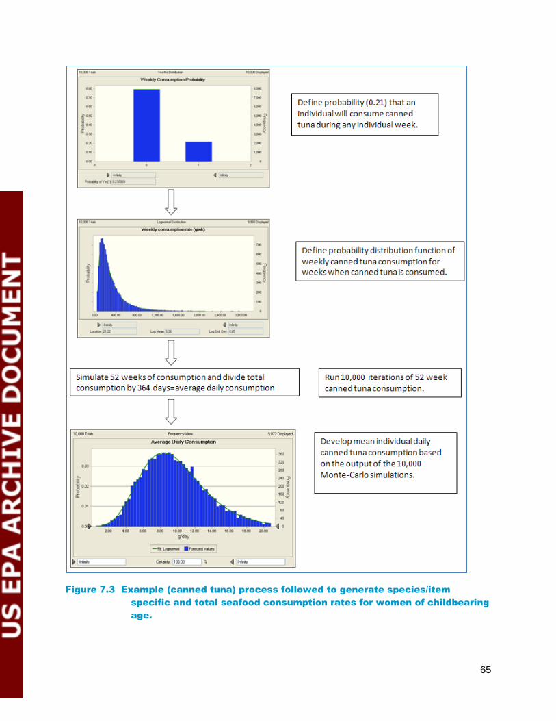
65

Figure 7.3 Example (canned tuna) process followed to generate species/item

specific and total seafood consumption rates for women of childbearing

age.

66

Figure 7.4. Average daily (g/day) canned tuna consumption rate distribution for

women of childbearing age. The distribution was developed based on

simulating 52 weeks of consumption for 10,000 individuals and

developing a composite distribution from the simulated individual daily

average consumption rates. Average daily individual consumption was

calculated as the sum across all 52 weeks divided by 364.

As described above, species/item specific consumption rate probability density functions were developed for canned tuna, shrimp, flounder, grouper, freshwater catfish, bread fish fillets, dolphin, stone crab claws, salmon, crab meat, oysters and scallops. Additionally, a probability distribution function was developed for total fish consumption. Consumption rates for the 42 occasionally consumed items were assigned proportionally based on the total fish consumption distribution function (Figure 7.5); that is, the simulated total consumption rate was multiplied by the percent total consumption rate for the given species (Table 7.1). For example, a woman whose simulated total consumption rate was 53 g/day would be assigned a seatrout consumption rate of 0.76 g/day (53 g/day x 0.0144). Species that individually accounted for less than 1% of the total consumption, for women of childbearing age, were aggregated into either other Florida seafood or other non-Florida seafood, based on whether the species occurred within Florida waters. Consumption rates for the aggregated other Florida and other non-Florida species were assigned proportionally based on the total consumption distribution. As in the previous example, a woman whose total consumption rate was 53 g/day would be assigned other Florida seafood and other non-Florida seafood consumption rates of 4.24(8% total) and 2.99 (5.65% total) g/day, respectively.

67

Figure 7.5. Average daily (g/day) total consumption distribution for women of

childbearing age.

Mean species specific tissue total mercury contamination levels were assigned to each species/item based on the best available data (Table 7.1). A distributional approach for characterizing tissue concentrations was considered, but not pursued based on the assumption that individual consumer exposure from any individual species would tend towards the mean concentration over the long-term. If mercury distributions had been included then the program would have randomly selected both species specific consumption rates and mercury contamination levels for each individual iteration with mercury exposures calculated as the product of the consumption rate and mercury contaminate level on a species basis. The species specific consumption rate assigned for each iteration really represents a long-term average daily consumption for that individual. The mercury contamination level should likewise reflect the long-term average level of mercury the individual is exposed to through consumption of the given species. Use of mercury contamination distributions would have assigned some individuals high contamination levels, which is equivalent to assuming that the particular individual’s exposure typically is at that level; however, exposure varies over time and by meal. For example, canned light chunk tuna mercury levels can range from 0.0 to 0.54 mg/kg with a mean of 0.11 mg/kg. It is highly unlikely that an individual who consumes tuna on a regular basis will always select (i.e., randomly pull from a store self) either the most or least contaminated cans of tuna, but will rather experience variation over time in exposure levels, such that the long-term exposure will tend towards a mean value. The species specific arithmetic mean values represent the best estimates of long-term exposures; therefore, consumption weighted mean tissue total mercury concentrations were calculated and used for the other categories of Florida and non-Florida seafood (Tables 7.2 and 7.3). Note: a more complex model incorporating variation in mercury content could be constructed, but such a model would require significantly more iterations as well as simulation of long-term individual exposure variation over a year or more.

68

Table 7.1 List of market basket species, consumption probability distribution

function or proportion (for occasionally consumed items) and mean Hg

tissue concentration. Probability distribution functions are listed in

Appendix J. Consumption rates for the remaining items were assigned

based on proportion of the total consumption distribution (lognormal

distribution).

Florida Species

Species Percent

Total Consumption

Mean Total Mercury (mg/kg)

Consumption Rate

N Canned tuna 24.00% 0.228 Distribution

Y Shrimp 9.97% 0.016 Distribution

Y Flounder 6.09% 0.115 Distribution

Y Snapper 5.92% 0.389 Distribution

Y Grouper 5.85% 0.489 Distribution

Y Freshwater catfish 4.20% 0.016 Distribution

N Breaded fish fillets 4.01% 0.010 Distribution

N Fish sticks 3.34% 0.010 Proportion of total

Y Mullet 3.13% 0.046 Proportion of total

Y Dolphin 2.53% 0.133 Distribution

Y Stone crab claws 2.45% 0.101 Distribution

Y Clams 2.23% 0.016 Distribution

N Salmon 2.09% 0.021 Distribution

Y Crab meat 1.91% 0.101 Distribution

Y Oysters 1.85% 0.011 Distribution

N Fresh tuna 1.61% 0.463 Proportion of total

Y Seatrout 1.44% 0.315 Proportion of total

Y Panfish 1.34% 0.204 Proportion of total

N Sardines 1.30% 0.013 Proportion of total

Y Scallops 1.07% 0.003 Distribution

Y Other FL Seafood 8.00% 0.428 Proportion of total

N Other Non-FL Seafood 5.65% 0.328 Proportion of total

(sources of average mercury: FWRI –Adams et al., 2003, FDA; Sunderland, 2012)

69

Table 7.2 Summary of calculation of consumption weighted mean total mercury

tissue concentration for the other Florida seafood category. Total

consumption was calculated as the total Degner survey reported

consumption for women of childbearing age.

Species Mean

Hg (mg/kg)

Total Consumption

(kg) Mean Hg ∙ Consumption Source

Amberjack 0.441 1305.6 576.19 FMRI

Blue crab 0.101 7288.4 734.02 FDA

King mackerel 1.153 1906.3 2198.54 FMRI

Mackerel 0.381 6988.4 2661.96 FMRI

Marine catfish 0.422 454.7 191.68 FDA/FMRI

Pompano 0.441 772.4 340.89 FMRI

Red drum 0.196 4510.9 885.26 FMRI

Salad shrimp 0.016 2918.1 47.58 FDA

Sheepshead 0.183 909.5 166.30 FMRI

Snook 0.374 893.9 334.59 FMRI

Whitefish 0.103 2303.8 237.46 FDA

Largemouth bass 0.470 7664.9 3602.50 Lange

Lobster tails 0.167 8084.8 1348.82 FDA

Shark 1.185 8389.4 9942.42 FDA/FMRI

Total

54391.1 23268.22

Weighted mean

0.428

Table 7.3 Summary of calculation of consumption weighted mean total mercury

tissue concentration for the other non-Florida seafood category. Total

consumption was calculated as the total Degner survey reported

consumption for women of childbearing age.

70

Total methylmercury exposure (dose) was calculated as the summed exposures for each item where the exposure of an individual item was calculated as the species specific consumption rate (kg/day) multiplied by the species/item specific mean total mercury contamination level (mg/kg, Equation 1). This use of total mercury, as normally measured, as surrogate for methylmercury adds a margin of safety as total mercury is always greater the methylmercury fraction. A distribution of exposures, based on 10,000 iterations, was generated for each scenario evaluated. Each individual iteration randomly selected a body weight, a total consumption rate, and seafood item specific consumption rates from the corresponding probability density functions (Appendix J). Exposure to mercury from the consumption of contaminated fish and seafood items is calculated as a function of consumption rate and the level of contamination present with the fish:

where,

FCi = Consumption of the ith species in kg/day, and TRCi = Tissue residual concentration (mg Hg/kg) of the ith species. For the Florida

market basket analysis, total residual concentration of the ith species were based on the mean tissue concentration for each species.

The Hg exposure was divided by the body weight (kg) to calculate the weight adjusted dose (mg Hg/kg∙day). For example, a woman of childbearing age consumes fish and other seafood items at the rates listed in Table 7.4. Her exposure to mercury from each item consumed is calculated by multiplying the consumption rate by the mercury contaminate concentration for the species. Her total exposure is calculated as the sum of the exposures from all species (Equation 1). The woman’s mercury dose is calculated as the total exposure to mercury by her

Species Mean

Hg (mg/kg)

Total Consumption

(mg/kg) Mean Hg ∙ Consumption Source

Bluefish 0.561 505.3 283.64 FDA/FMRI

Halibut 0.232 365.8 84.93 FDA

Mussels 0.030 2306.4 69.19 Sunderland

Sea bass 0.218 480.7 104.98 FDA/FMRI

Swordfish 1.088 6828.6 7426.10 FDA

Whole lobster 0.167 7496.0 1250.59 FDA

Cod 0.113 6663.7 751.19 FDA

Haddock 0.057 1336.1 76.54 FDA

Imitation crab meat

0.010 6813.1 65.15 FDA

Orange Roughy 0.569 2710.0 1543.22 FDA

Total

35505.5 11655.55

Weight mean

0.328

Equation 1

71

body weight (Equation 2). The example women weighs 63 kg, thus her dose is 0.13 mg Hg/kg∙day. The dose is compared to the reference dose (RfD) of 0.10 µg Hg/kg∙day, leading to the conclusion that the woman exceeds the reference dose.

Table 7.4. Example calculation of mercury exposure and dose

Species FCi (Consumption Rate,

kg/day)

TRCi (Tissue Hg

Concentration, mg Hg/kg)

Hg Exposure (THg) (mg Hg/day)

Canned tuna 0.0092 0.228 0.0021 Shrimp 0.0037 0.016 0.000060 Flounder 0.0013 0.115 0.00015 Snapper 0.0037 0.389 0.00144 Grouper 0.0025 0.489 0.00120 Freshwater catfish 0.0010 0.016 0.00002 Breaded fish fillets 0.00020 0.010 0.0000019 Fish sticks 0.0015 0.010 0.000014 Mullet 0.0014 0.046 0.000063 Dolphin 0.0010 0.133 0.00014 Stone crab claws 0.00046 0.101 0.000046 Clams 0.00097 0.016 0.000015 Salmon 0.0016 0.021 0.000034 Crab meat 0.0008 0.101 0.000081 Oysters 0.00071 0.011 0.000008 Fresh tuna 0.00071 0.463 0.00033 Seatrout 0.00063 0.315 0.00020 Panfish 0.00059 0.204 0.00012 Sardines 0.0006 0.013 0.0000075 Scallops 0.0004 0.003 0.0000015 Other FL Seafood 0.0035 0.428 0.0015 Other non-FL Seafood 0.0025 0.328 0.00081

Total Exposure (mg Hg/day) 0.00832

Dose (µg Hg/kg∙day) 0.132

Monte Carlo analysis conducts repeated random samplings from a population or distribution to compute a range of outcomes based on variability in the input variables. In the case of the mercury market basket analysis repeated samplings were conducted from the distributions of species specific consumption rates (FCi) and body weights for women of childbearing age (BWj), where BWj is the body weight in kilograms for the jth woman. Mercury doses were calculated for each randomly selected combination of body weight (BWj) and fish consumptions (FCi), resulting in a distribution of mercury doses for Florida women of childbearing age. The

Equation 2

72

distributions used in the analysis are summarized in Appendix J. All Monte Carlo analyses were conducted for 10,000 iterations. DEP evaluated the sensitivity of the analysis (exposure distribution) to the number of iterations. Analyses conducted using 50,000 and 100,000 did not produce significantly different results at the mean, 90th, or even 95th percentile of the exposure distribution. It was therefore determined that 10,000 iterations were sufficient to provide a stable solution to the problem. An analysis of baseline or current conditions (current mean methylmercury contamination levels) suggested that there is a 51.5% certainty that the target population (women of childbearing age) is at or below the protective reference dose of 0.1 µg/ kg∙day (Figure 7.6). This level of certainty indicates that a significant portion of the population could exceed the reference dose and may be at risk of adverse health effects. The analysis shows that women of childbearing age are under-protected at the existing mercury contamination levels in fish they consume.

73

Figure 7.6 Baseline scenario cumulative probability distribution of methyl mercury

dose for women of childbearing age based on the market basket

analysis.

The Monte Carlo simulator was next used to evaluate the effect of reducing Florida fish contamination levels on the dose distribution. This analysis involved iteratively reducing the tissue residual concentration (TRCi) for Florida species by a constant percentage and running the Monte Carlo analysis of body weights and consumption rates until a 90% certainty of not exceeding the reference dose was achieved. The randomly sampling was conducted in the same manner as was done for the baseline analysis. This analysis found that Florida fish levels would need to be reduced to 40% of current levels (i.e., 60% reduction) to achieve the protective target certainty level (Figure 7.7). Under the Florida species 60 percent reduction scenario the previous example 63 kg woman from Table 7.4 would now receive a dose of only 0.084 µg Hg/kg∙day, which is below the RfD (Table 7.5). This 60% reduction in total sources is equivalent to an 86% reduction in anthropogenic sources given that natural background deposition accounts for 30% of the deposition. These results are supported by the Department’s independent study (Sunderland et al., 2012) looking at fish consumption and exposure for Gulf of Mexico residents, which using a larger list of species consumed (N=32) and applying a similar probabilistic approach, found similar exposures, and thus similar reductions in anthropogenic sources being required to reduce exposure.

Table 7.5. Mercury exposure and dose for the example women from Table 7.4. The

example woman weighs 63 kg and consumes fish and seafood items

according to the patterns listed in FCi column below. Mercury exposures

were calculated based on the FL species reduction scenario tissue

concentration levels.

Florida Species

Species FCi (Consumption Rate, kg/day)

Baseline TRCi

(Tissue Hg Concentration,

mg Hg/kg)

FL Species Reduction Scenario

TRCi (Tissue Hg


Hg Exposure (mg Hg/day)

N Canned tuna 0.0092 0.228 0.228 0.0021

Y Shrimp 0.0037 0.016 0.007 0.000024

Y Flounder 0.0013 0.115 0.046 0.000059

Y Snapper 0.0037 0.389 0.156 0.00058

Y Grouper 0.0025 0.489 0.196 0.00048

Y Freshwater catfish 0.0010 0.016 0.006 0.0000064

N Breaded fish fillets 0.00020 0.010 0.010 0.0000019

N Fish sticks 0.0015 0.010 0.010 0.000014

Y Mullet 0.0014 0.046 0.018 0.000025

Y Dolphin 0.0010 0.133 0.053 0.000055

Y Stone crab claws 0.00046 0.101 0.040 0.000019

74

Florida Species

Species FCi (Consumption Rate, kg/day)

Baseline TRCi

(Tissue Hg Concentration,

mg Hg/kg)

FL Species Reduction Scenario

TRCi (Tissue Hg


Hg Exposure (mg Hg/day)

Y Clams 0.00097 0.016 0.006 0.0000061

N Salmon 0.0016 0.021 0.021 0.000034

Y Crab meat 0.0008 0.101 0.040 0.000032

Y Oysters 0.00071 0.011 0.005 0.0000032

N Fresh tuna 0.00071 0.463 0.463 0.00033

Y Seatrout 0.00063 0.315 0.126 0.000079

Y Panfish 0.00059 0.204 0.082 0.000048

N Sardines 0.0006 0.013 0.013 0.0000075

Y Scallops 0.0004 0.003 0.001 0.00000061

Y Other FL Seafood 0.0035 0.428 0.171 0.00060

N Other Non-FL Seafood

0.0025 0.328 0.328 0.00081

Total Exposure (mg Hg/day) 0.00530

Dose (µg Hg/kg∙day) 0.084

75

Figure 7.7 Sixty percent reduction in Florida species methyl mercury scenario

cumulative probability distribution of methyl mercury dose for women of

childbearing age based on the market basket analysis.

The 60% reduction and 90% certainty assume no change in non-Florida species; however, U.S. EPA and other states are simultaneously seeking mercury source reductions. Therefore, it is highly likely that reductions in non-Florida seafood will occur and result in even greater certainty of achieving the reference dose. Furthermore, 403.067(6), F.S., requires the Department to consider the extent to which nonattainment of water quality standards is caused by pollution sources outside of Florida when allocating TMDLs. DEP ran a series of scenarios assuming reduction in non-Florida species to maximum target contamination levels ranging from 0.1 mg/kg to 0.3 mg/kg. Under these scenarios, the mean methyl mercury level for any species above the maximum target level was reduced to the target level. For example, mean canned tuna is currently at 0.228 mg/kg. Under the 0.1 mg/kg scenario the assumed contamination level was reduced to 0.1 mg/kg. The non-Florida species reduction scenarios were applied in addition to an assumed 60% reduction in Florida species. The analysis showed that reductions below 0.2 mg/kg in non-Florida species substantially increased the certainty (Table 7.4) that the protective reference dose will be achieved. Specifically, reductions in non-Florida species to 0.15 mg/kg or less will result in a greater than 99% certainty.

76

Table 7.6 Summary of baseline (current condition) and reduction scenario methyl

mercury exposure risks. Certainty represents the confidence that the

population is at or below the reference dose (0.1 µg/kg∙day). Reduction

scenarios were run by reducing fish tissue concentrations by a reductions

factor (i.e., RF*species mean concentration) necessary to achieve 90

percent certainty assuming no reduction in non-Florida species.

Additional scenarios were run under the assumptions that non-Florida

species are reduced to levels ranging from ≤0.10 to 0.3 mg/kg.

Florida Species Percent Reduction

Non-FL Species Max. mg/kg

Certainty

Baseline Baseline 51.50

60 Baseline 90.18

60 0.300 91.96

60 0.275 93.07

60 0.250 92.80

60 0.225 94.52

60 0.200 96.63

60 0.175 98.35

60 0.150 99.39

60 0.125 99.79

60 0.100 99.92

7.1.1.2 Using Largemouth Bass:

A second line of evidence for setting a TMDL reduction target is to assess the data gathered statewide for top trophic level predators that live in most of Florida’s waterbodies and are consumed by humans. For marine species, Snapper and Grouper represent the highest consumed, top trophic level species that exist in Florida waters. Largemouth bass (LMB) represents the highest consumed, top trophic level species that exist in Florida’s freshwater lakes and streams. The average mercury concentration of these species is relatively equivalent. Because the State has much more data for LMB, we will focus on that species as a surrogate for the statewide (fresh and marine) TMDL targeting. Beginning in 1983, and under contract with the Florida Fish and Wildlife Conservation Commission, the DEP has been provided with 31,159 fish tissue samples, mostly targeting Largemouth Bass (LMB). For the purposes of setting this Total Maximum Daily Load, a stratified-randomized sampling approach was designed and implemented for the period 2008-2010, also focusing on LMB. While the DEP has mercury data for many fish species, a reduction target based on a high trophic level predator (such as LMB) will be protective of all the other lower trophic level feeders. As was not the case with the fish tissue data collected prior to 2008, a specific suite of water chemistry was also collected to aid in our assessment of the potential causes of methylation in Florida’s fresh surface waters. Having these paired water quality data also allowed us to calculate a “Bioaccumulation Factor” for each waterbody, and from these values, an average statewide BAF was determined.

77

Previously, other states, and groups of states, have established statewide (or regional) TMDLs for mercury as a way to efficiently address widespread fish consumption advisories. New Jersey recently (2009) had approved a TMDL for 122 waterbodies listed as impaired for mercury in fish tissue, with sources that were tied to air emissions (TMDL for Mercury Impairments Based in Concentration in Fish Tissue Caused Mainly by Air Deposition to Address 122 HUC 14s Statewide, NJDEP, 2010). As was done in the TMDLs for New Jersey, and by applying the assumption of a linear relationship between mercury in the environment to that in fish tissue, the needed reduction in mercury deposition can be calculated. Specifically in Florida, if the required reduction is based on the 90th percentile concentration of mercury in LMB measured over the designated study period (i.e., a value of 0.74 mg/Kg for the period 2008-2010) and compared to the desired fish tissue target of 0.3 mg/Kg for the general population, a reduction of 85% of anthropogenic sources contributing to Florida’s mercury burden would have to be achieved.

7.2 Reduction Target for Fish Consumption by Wildlife

Wildlife may be at risk of mercury exposure from consumption of fish with elevated levels of mercury. The greatest risk is for piscivorous species. In the Mercury Report to Congress, a value of 0.077 ppm was deemed as being protective of Trophic Level-3 wildlife consumers and 0.346 for Trophic Level-4 wildlife consumers. For this analysis, the more protective value of 0.077 is used herein to evaluate necessary reductions in mercury sources for the protection of wildlife. The Department focused its evaluation on Wood Storks (Mycteria americana), and Great Blue Herons (GBH, Ardea herodias) as the primary though not exclusive focus. White Ibis (Eudocimus albus), and other smaller wading birds such as Tricolor Herons (Egretta tricolor), Little Blue Herons (Egretta caerulea), and others, were also considered but as the smaller wading birds are primarily feeding on Trophic Level-2 prey items, it is considered that if the target value of 0.077 is achieved for wood storks and GBH, then lower trophic levels would similarly be protected. This setting of reduction targets based upon a higher trophic level follows guidelines of USEPA, and approaches used in promulgated mercury TMDLs. Based upon the monitoring performed for the Mercury TMDL project (see Chapter 5 and Appendix H) an evaluation by system type of stream/river, lakes/ponds, and Everglades, the Everglades has the highest levels of mercury as observed in LMB (Figure 7.8).

Figure 7.8 Box plot (left) and cumulative frequency distribution plot (right) comparing

standardized (15 inch length) largemouth bass (LMB) total mercury

78

concentrations in fish tissue collected in the Everglades measured from

2008–2010. Box plots represent median and 25th, and 75th percentiles;

whiskers represent 10th and 90th percentiles; and points are outliers.

Sample numbers are as follows: Everglades = 32, Florida lakes = 130, and

streams = 120 (Axelrad, D., et al., 2012)

Thus, assessing trophic level-3 fish in the Everglades, as may be consumed by Wood Storks and GBH, provides a margin of protection to other system types across the state. The Everglades Protection Area has numerous wood stork rookeries (Figure 7.9), and GBH rookery and loafing areas are ubiquitous across the region.

Figure 7.9 Wood Stork Rookeries and Foraging Areas in Everglades Protection Area

Wood stork rookeries are provided as the foraging region of wood storks are known to be most limited of the two demonstration species. Foraging for wood storks during late phases of the nesting season track well with water drawdowns in forage areas (thereby concentrating food species). This provides concentrations that allow easier capture of smaller individuals relative to level of effort. Fish size consumed is normally 1-6 inches in length.

2000

2001

2002

2003

2004

2005

2006

2007

2008

2009

2010

2011

EvPA T

L3 F

ish T

Hg (

mg/k

g)

0.0

0.1

0.2

0.3

0.4

0.5

0.6

0.7

0.8

79

Figure 7.10 Mercury in TL3 fish (bluegill, redear sunfish, and spotted sunfish)

collected from 25 locations in the Everglades Protection Area from

2000 to 2011. Data include the median (black horizontal line), mean (red

horizontal line), 25-75th

percentiles in yellow, 10-90th

percentiles as

whiskers, and 5-95th

percentiles as points.

The mean mercury level in TL3 fish across the Everglades Protection Area is 0.176 mg/kg (N = 1,966). This number is used analogously to the average mercury values used in fish species in the Market Basket approach presented earlier as to evaluating fish consumption risk in the at risk population of women of childbearing age and young children. The margins of safety inherent in the use of the average for wading bird consumption include: diets are not exclusively fish, diets are skewed toward fish smaller than those collected for measuring THg in fillets, and whole fish values for mercury are typically lower than fillet-only values (Bevelhimer et al., 1997). The latter is true due to limited concentration of mercury in bones, as compared to other metals such as arsenic, as well as limited sequestration in organs. Applying the more conservative percent reduction, i.e., higher value, as determined in the anthropogenic exposure evaluations, of 60%, the respective reduction in TL3 fish would result in an expected level of:

0.176 mg/kg * 0.60 (percent reduction) = 0.070 mg/kg Concerns for individual hot spots within the Everglades Protection Area are at times raised relative to wildlife exposure through fish consumption. However, in terms of practical application when one considers foraging patterns, that “hot spots” are being driven as coincident with single sampling events, and that hot spot locations do not remain stationary across time – further indicating that these location representations are sampling artifacts -, hot spots are not deemed to be an established control point for exposure. If one were to consider a single hot spot location then this would have to visited repeatedly, with the same elevated level being experienced by the same bird at each feeding. For GBH and other wading birds there is not same focus on common forage location that there is for wood storks. GBH breeding adults range as much as 30 km from the colony, and typically range 6.5 km (Butler, 1992), areas much larger than “hot spots.” Other large charismatic species such as Great Egrets (Ardea alba) forage primarily on nekton, crustaceans, and other aquatic invertebrates (Kushlan, 2000). The size of other wading birds limits opportunity to feed on larger fish that are of a size and age to have accumulated elevated levels of mercury. The Everglades marsh limits fish foraging to wading birds. The potential of visiting a hot spot is the same as any other single location in the landscape. The above factors combine to limit risks of “hot spots” for non-wood storks. For wood storks, the focus on location is coincident with water level drawdowns concentrating prey fish, and primary fish consumed being smaller fish. The wider area upon which fish population concentration is based during draw downs eliminates point measures of hot spots, as well as increases concentration of small prey items, i.e., more small fish are comprising the diet during drawdowns. Thus, the depressional areas in which wood storks forage later in nesting season represent much larger areas of recruitment of prey items as a consequence of lower water levels concentrating regional prey distributions. Thus, the hot spot phenomena, as a basis of elevated exposure, is also moot for wood storks.

7.3 Demonstration of Protection of Water Quality Standards

80

The Department of Environmental Protection is charged with developing Total Maximum Daily Loads that demonstrate the expected reductions, when achieved, will result in attainment of its water quality standards. As the DEP currently lacks a mercury in fish tissue criterion, evidence must be provided to show that the fish tissue target established under this TMDL will be protective of the water quality criteria found in Chapter 62-302.530(41), Florida Administrative Code. Using the fish tissue mercury concentration and ambient methylmercury and total mercury concentration data collected from 264 Florida streams and lakes in the period from 2008 through 2010, the Department concluded, based on a Monte Carlo analysis, that, once the 0.3 mg/Kg fish tissue concentration target is achieved, there is a 95 percent probability that the ambient total mercury concentration in freshwater systems in the State of Florida would be lower than the 12 ng/L ambient total mercury criteria for freshwater systems. This demonstrates with a high confidence level that the statewide mercury TMDL will be protective of the ambient water quality criteria. The same mercury load reduction will also be protective of Florida marine waters, which has a total mercury ambient target of 25 ng/L. Detailed descriptions on the analysis can be found in Appendix M.

Chapter 8: Determination of the TMDL

8.1 Expression and Allocation of the TMDL

The objective of a TMDL is to provide a basis for allocating acceptable loads among all of the known pollutant sources in a watershed so that appropriate control measures can be implemented and water quality standards achieved. A TMDL is expressed as the sum of all point source loads (wasteload allocations, or WLAs), nonpoint source loads (load allocations, or LAs), and an appropriate margin of safety (MOS), which takes into account any uncertainty concerning the relationship between effluent limitations and water quality:

TMDL =

As discussed earlier, the WLA is broken out into separate subcategories for wastewater discharges and stormwater discharges regulated under the NPDES Program:

TMDL wastewater + NPDES Stormwater +

It should be noted that the various components of the revised TMDL equation may not sum up to the value of the TMDL because (a) the WLA for NPDES stormwater is typically based on the percent reduction needed for nonpoint sources and is also accounted for within the LA, and (b) TMDL components can be expressed in different units (for example, the WLA for stormwater is typically expressed as a percent reduction, and the WLA for wastewater is typically expressed as mass per day). WLAs for stormwater discharges are typically expressed as “percent reduction” because it is very difficult to quantify the loads from MS4s (given the numerous discharge points) and to distinguish loads from MS4s from other nonpoint sources (given the nature of stormwater transport). The sources of mercury in a stormwater collection system are from wet and dry deposition, and atmospheric deposition is considered a component of the nonpoint source load allocation. This approach is consistent with federal regulations (40 CFR § 130.2[I]), which state that TMDLs can be expressed in terms of mass per time (e.g., pounds per day), toxicity, or other appropriate measure. Florida’s TMDL for mercury is expressed in terms of a percent reduction, and represents the maximum daily load Florida’s lakes, streams, estuaries, and coastal waters can assimilate without exceeding the water quality criteria for mercury (Table 8.1).

8.2 Load Allocation

A reduction in mercury of 86 percent is needed from nonpoint sources contributing to all of the fresh and marine waters in Florida to address our water quality limited segments and to protect public health. As this reduction is expressed as a percent, the value is applicable over any time period, and thereby meets EPA’s requirement that TMDLs must be expressed as a “daily” value. It should be noted that the LA includes loading from stormwater discharges regulated by the Department and the water management districts that are not part of the NPDES Stormwater Program (see Appendix K). As the predominant nonpoint source of mercury to Florida’s waters arrives via atmospheric deposition, from sources both within and outside of Florida, specific allocations cannot be made at this time. This 86 percent reduction is needed both within and

82

outside of Florida and does not preclude consideration of reductions already being achieved by Florida sources as identified in Chapter 9. Reductions, as deemed necessary and practicable (recognizing technological, fiscal, and legal constraints) will be assigned during the subsequent TMDL implementation phase, described more completely in Chapter 9.

Table 8.1 TMDL Components for Mercury in Florida’s Fresh Water Lakes, Streams,

and Estuarine and Coastal Waters8

This is a six-column table. Column 1 lists the parameter, Column 2 lists the TMDL, Column 3 lists the WLA for wastewater, Column 4 lists the WLA for NPDES stormwater, Column 5 lists the LA (percent

reduction), and Column 6 lists the MOS.

Parameter TMDL

(% reduction)

WLA for Wastewater

(Kg/year)

WLA for NPDES Stormwater

LA (% reduction)

MOS

Mercury 86 23 kg* ** 86 Implicit

* Based on all readily available data, the Department estimated the current permitted mercury load being discharged to waters of the state. This value represents less than 0.5 % of the total mercury load from point and nonpoint sources in Florida. Mercury minimization is expected for major facilities.

** NPDES MS4 Permits may require reductions to meet the TMDL goal if sources of mercury under the direct control of a MS4 permittee or co-permittee are found to exist.

8.3 Wasteload Allocation

8.3.1 NPDES Wastewater Discharges

The WLA for the mercury TMDL is established as 23 kg/year. This value translates to 0.063 Kg/day. Consistent with the findings of other approved TMDLs established on a regional, statewide, or multi-state basis, Florida has determined that the mercury contribution from NPDES-permitted point source discharges are minor relative to the loads being deposited on Florida’s land and waters (fresh and marine) from atmospheric deposition. In Florida, the existing point source load for the entire state has been estimated as being approximately 0.5 % of the total mercury loading to the land and waters of the state. According to EPA’s Guidance for Implementing the January 2001 Methylmercury Water Quality Criterion (EPA, 2010), point source discharges are considered a small contribution if the loading or cumulative loading of all point sources to the receiving water are expected to account for a small or negligible portion of the total mercury loadings. Table 8.2 provides a summary of the fraction the proposed Wasteload Allocation for NPDES permitted facilities versus the existing total mercury load for Florida and how those values compared to statewide or regional mercury TMDLs approved elsewhere in the United States. The Department anticipates that the significant decreases in mercury loading to Florida’s waters have been and will continue to be associated with reductions in atmospheric emissions from anthropogenic sources within and outside of Florida.

8 To the extent that this draft reads as though it applies to more than the WBIDs in Appendix A, this proposal only applies to the WBIDs in Appendix A.

83

Table 8.2 TMDL Comparison of Wasteload Allocations for Mercury as a Percentage

of Total Mercury Load for Florida and Other State or Regional TMDLs

State or Region Total Mercury Load Wasteload Allocation WLA/Total Load (%)

Minnesota 2781 Kg/yr 11 Kg/yr 0.40

Northeastern States 6,651 Kg/yr 38 Kg/yr 0.57

New Jersey 601 Kg/yr 6.8 Kg/yr 1.13

Florida 4,793 Kg/yr 23 Kg/yr 0.48

Once this TMDL is in effect, any new requirements will generally be evaluated and addressed in the renewal of existing NPDES permits for point sources, if not earlier through a reopener clause. The need for compliance schedules to meet the TMDL requirements may be established in a BMAP and/or in NPDES permits or an associated Administrative Order. In cases where there are sufficient data to determine whether the NPDES discharger has quantifiable concentrations of mercury, NPDES permits except domestic facilities discharging less than 1 MGD will include a set of additional conditions for implementation of a mercury minimization program to ensure that point sources are discharging the minimum amount of mercury practicable. For domestic facilities with quantifiable concentrations of mercury and discharging greater than 1 MGD, a mercury minimization plan shall include annually the identification of dental operations, hospitals and educational facilities (i.e., Universities and K-12 schools) within their service area; the production or adoption of best management practices (BMPs) for the appropriate industries as applicable; and promulgation of the BMP program. This option will meet the applicable federal regulatory guidance and requirements (EPA, 2010). All of the NPDES-permitted domestic wastewater facilities were assessed using data available the WAFR database (as of July 2012) and the combined permitted flows were calculated. The result of combining the permitted flows from domestic facilities (1353 MGD) with those for the industrial facilities (785 MGD) yielded a total of 2138 MGD. In addition, the permitted industrial wastewater flows were also calculated, but with two caveats. First, not all of the industrial facilities have permit limits for flow. Second, for power plants that use once-through cooling water, those volumes were calculated separately from the total for other industrial sources. It is also presumed that “Intake Credits” can be provided for any mercury that is passing through the facility via once-through cooling water. However, other waste streams (e.g., discharges from coal ash storage facilities or ponds) are not excluded from subsequent investigations, whose findings may be addressed in mercury minimization plans.

8.3.2 NPDES Stormwater Discharges

The WLA for stormwater discharges with an MS4 permit has been determined to be generally not applicable. Any MS4 permittee is only responsible for reducing the anthropogenic loads associated with stormwater outfalls that it owns or otherwise has responsible control over, and it is not responsible for reducing other nonpoint source loads in its jurisdiction. Therefore, as the mercury levels that may be present in stormwater are a result of nonpoint sources linked to atmospheric deposition, no reductions are required of the MS4 permittees in Florida. However, if through the course of monitoring or in light of other information becoming available, local sources of mercury under the control of the MS4 permittee or a co-permittee are found to exist,

84

the permit holder will be subject to implementing necessary controls to reduce mercury loads associated with those local sources, so as to meet the requirement of this TMDL.

8.4 Margin of Safety

There are multiple lines of evidence to support the use of an implicit margin of safety in this TMDL. Consistent with the recommendations of the Allocation Technical Advisory Committee (Department, 2001), an implicit MOS was used in the development of this TMDL. Included in this implicit MOS is the assumption that all of the mercury in fish tissue is in the form of MeHg (the harmful fraction) and it is not. As discussed in Section 2.2, the application of a multifold increase in setting of the reference dose for MeHg is another significant component of the Margin of Safety (MOS). As noted previously, compared to other fish species, Largemouth Bass have higher overall tissue MeHg concentration because their position in the food chain dictates a longer food chain length for bioaccumulation. Use of Largemouth Bass for the TMDL target development provides another margin of safety to the TMDL as all other fish living at lower trophic levels will also benefit.

85

Chapter 9: Ongoing Activities and Implementation

Plan Development

9.1 Implementation Plan Development

Following the adoption of this TMDL by rule and adoption or approval by EPA, the Department will determine the best course of action regarding its implementation. The TMDL alone does not create new legal authorities and the LA and WLA discussed herein are enforceable to the extent independent legal authorities exist under state law. In general and depending on the pollutant(s) causing the waterbody impairment and the significance of the waterbody, the Department will select the best course of action leading to the development of a plan to restore the waterbody. Agency actions to implement this TMDL are subject to Section 403.067, Florida Statutes as well as the notice and hearing processes of Chapter 120 of the Florida Statutes. Implementation can be accomplished cooperatively with stakeholders by creating a Basin Management Action Plan, referred to as the BMAP. BMAPs are one mechanism through which TMDLs are implemented in Florida (see Subsection 403.067[7], F.S.). If the Department determines that a BMAP is needed to support the implementation of this TMDL, a BMAP will be developed through a transparent, stakeholder-driven process intended to result in a plan that is cost-effective and technically feasible, and that meets the restoration needs of the applicable waterbodies. Once adopted by order of the Department Secretary, BMAPs are enforceable through wastewater and municipal stormwater permits for point sources and through BMP implementation for nonpoint sources. However, in some basins and for some parameters the development of a BMAP is not the most efficient way to restore a waterbody such that it meets its designated uses. This is because some impairments result from the cumulative effects of a multitude of potential sources, both natural and anthropogenic. The Department can rely on existing permitting programs, local or industry initiatives, or a combination of both as a more cost-effective and simplified approach to identify the actions needed for restoration activities, while still meeting the requirements of Subsection 403.067(7), F.S.

9.2 Ongoing Mercury Reduction Activities in Florida

An important element of implementation planning is consideration of mercury reductions already in place or in progress as well as the cost effectiveness of minimization efforts. Global anthropogenic emissions of mercury are the source of the vast majority of mercury deposition in Florida. Thus, Florida’s achievement of the TMDL is dependent upon not only out-of-state but out-of-country mercury emission reductions. Florida sources are, however, implementing mercury reduction efforts that must be taken into account. On the point source side, many NPDES Industrial and Domestic Permitted Sources are already regulated for mercury and it is anticipated EPA will be revising its effluent limitation guidelines to further limit discharges of metals from some source categories. On the non-point source side, as discussed previously, there has been a significant reduction in air emissions of mercury from Florida facilities. In addition, there are also numerous, ongoing waste reduction efforts being implemented to reduce mercury from Florida’s waste stream.

86

Mercury Waste Reduction Strategies in Florida Florida is a recognized leader among states in managing mercury waste and reducing its use in products. Florida’s statutes and rules governing mercury predate federal regulations and helped drive national policy. DEP Waste Management Program involvement is characterized with the following activities which are also described with more detail below. The list starts with programs currently having the most potential or actual impact on reducing mercury in Florida’s environment. • Reducing mercury from batteries through legislation • Promoting recycling of mercury containing lamps and devices through regulation and education • Helping operators safely use drum top crushers according to regulation for volume reduction of spent fluorescent lamps • Recycling mercury from homeowners and Conditionally Exempt Small Quantity Generators through Florida’s Household Hazardous Waste program • Providing a convenient mercury recycling agreement for state and municipal agencies • Innovatively reducing mercury use in hospitals, • Providing mercury thermometer exchange programs, • Adopting the Thermostat Recycling Corporation (TRC) program and leading in the nation in recycling mercury thermostats, • Participating in the national End of Life Vehicle Solutions (ELVS) program for auto mercury • Creating a mercury amalgam management BMP brochure, • Requiring recycling of mercury-containing lamps and devices in the Green Lodging program, • Requiring recycling of bilge pump switches in the Clean Marina program, • Recommending removal of mercury-containing lamps and devices from buildings prior to demolition, • Developing beneficial reuse of fluorescent lamp glass generated through recycling • Providing data on metal loading in ash and leachate from ash disposal Federal legislation has also helped reduce mercury waste in Florida. Florida has adopted the Universal Waste Rule to help manage waste mercury and ensure its proper recycling. The federal ban on sale of mercury fever thermometers has helped eliminate one of the largest sources of mercury in the home.

87

Regulations and Statutes Chapter 62-737, Florida Administrative Code, titled “The Management of Spent Mercury-Containing Lamps and Devices Destined for Recycling” details requirements for recycling and has contributed to better management of mercury waste in Florida. Statutory authority for the environmentally sound management of mercury-containing lamps and devices, elimination of mercury in packaging, and elimination of mercury from batteries sold in Florida (Sections 403.7186, 403.7191, and 403.7192, Florida Statutes, respectively) have been important components of proper mercury waste management in Florida. Rules and Statutes pertaining to mercury can be found at: http://www.dep.state.fl.us/waste/categories/mercury/pages/laws.htm. Regulations from other states have also helped mercury waste management in Florida. An example is the strict labeling regulations adopted in some New England states. Product manufacturers have used labeling on products sold nation-wide as a result which helps show Florida consumers what products contain mercury and should be recycled. Reduction of Mercury from Batteries Legislation [403.7192, Florida Statutes] sets limitations on the mercury content of alkaline-manganese/zinc-carbon batteries and button batteries; prohibits sale of button-shaped batteries with a mercury electrode; and establishes a disposal ban and take back requirements for other batteries with a mercury electrode. This has resulted in a reduction of mercury in municipal solid waste and a concomitant reduction in mercury content in sentinel species, primarily freshwater fish and wading birds. Mercury-Containing Lamps Recycling No report on mercury management in Florida would be complete without discussing how lamps are recycled. Florida currently has one permitted mercury reclamation/recovery facility, one permitted mercury recovery facility, and a third mercury recovery facility in the permitting process. This means we have the ability to recycle our mercury in-state and keep recycling costs lower for our regulated community. Handler/transporter businesses register with the Department to provide more transparency in their operations. Drum Top Crushers for Fluorescent Lamps Another aspect of lamp recycling in Florida is the use of drum top crushers (DTC) for fluorescent lamps. These devices can be used for recycling a generator’s lamps on site. The ease of operation and convenience make them a popular method of lamp management in Florida, and facilities with storage issues find them particularly appealing. A 2010 interpretation of 62-737.400(6)(b), F.A.C., resulted in an additional use memo that allows a DTC to be put on a truck and taken to the generator’s site. At least one company is using this to recycle the copious numbers of lamps generated at tanning salons, a class of generators that have historically not recycled their lamps. The memo and other information about drum top crushers is here: http://www.dep.state.fl.us/waste/categories/mercury/pages/drum-top.htm Household Hazardous Waste Program The Department’s strong state-wide Household Hazardous Waste program has been an important contributor to the recycling of mercury statewide. Thermometers, fluorescent lamps, thermostats, other mercury containing devices and even bottles of elemental mercury have been properly recycled and kept out of the waste stream. The HHW web pages are here: http://www.dep.state.fl.us/waste/categories/hazardous/pages/household.htm .

http://www.dep.state.fl.us/waste/categories/mercury/pages/drum-top.htm

http://www.dep.state.fl.us/waste/categories/hazardous/pages/household.htm

88

Recycling Agreement for State and Municipal Government Entities The Florida Department of Management Services has provided a State Purchasing Agreement for municipal and state government facilities to recycle their mercury-containing lamps and devices at a competitive price. The State Purchasing Agreement that is renewed annually can be viewed here: http://www.dep.state.fl.us/waste/categories/mercury/pages/contract.htm. Hospital Mercury Reduction Program Starting in 1998, various hospitals were visited and received recycling information and, more importantly, information on alternatives to mercury-containing devices. Presentations at conferences for hospital waste management personnel also helped disseminate this information. Hospitals learned how to store and recycle their mercury-containing lamps and devices. Perhaps the most important component was a strong push to eliminate the use of mercury sphygmomanometers. Working with the national programs Hospitals for a Healthy Environment and Healthcare Without Harm brought additional resources to Florida’s hospitals. The Department also worked with Florida’s Department of Health to write a letter banning the use of mercury sphygmomanometers in Florida’s health clinics, resulting in the recycling of these devices as they have been replaced with mercury-free alternatives. Two reports on the medical program can be found here: http://www.dep.state.fl.us/waste/categories/mercury/pages/medical_facilities.htm . Staff continues to work with Hospitals for a Healthy Environment as a reviewer and judge for their “Making Medicine Mercury Free” annual national awards program. Thermometer Exchange Programs The Department’s Pollution Prevention efforts helped develop more mercury awareness by holding and participating in mercury thermometer exchange programs in various parts of the state and also through programs during Earth Day celebrations. These collection programs were an important step that preceded the federal ban on sale of mercury fever thermometers for home use. Thermostat Recycling Corporation Participation in Florida Thermostat Recycling Corporation is a national product stewardship program. Member heating, ventilation and air conditioning (HVAC) contractors and wholesalers can use the program to send mercury thermostats for recycling at no cost. Since its inception, Florida has led the country in number of participating wholesalers and in thermostats recycled. Recently many of our Household Hazardous Waste programs have also become TRC members, broadening the reach of the program. The website for the national program is http://www.thermostat-recycle.org/pages/the-program Automotive Mercury Recycling A small amount of mercury has historically been used in automobiles. Small ampoules are used in tilt switches in anti-lock brake systems (ABS), trunk lighting systems and sometimes in hood lighting systems. Although they have been engineered out of most vehicles, millions of vehicles are still in operation with these switches intact. As they aged, the majority of them were being sent to scrap yards with the mercury still in the vehicle until a national program was set up in 2000 to capture these small ampoules for recycling. ELVs (End of Life Vehicle Solutions) even provided a bounty for the switches until their funds expired. This program has helped keep tons of elemental mercury out of the waste stream nationwide. Florida has collected at least 318.15 pounds of mercury from over 145,000 switches to date. More information is available at http://www.elvsolutions.org/ .

http://www.dep.state.fl.us/waste/categories/mercury/pages/contract.htm

http://www.dep.state.fl.us/waste/categories/mercury/pages/medical_facilities.htm

http://www.thermostat-recycle.org/pages/the-program

http://www.thermostat-recycle.org/pages/the-program

http://www.elvsolutions.org/

89

Dental Amalgam Management Guidance In 2000, Florida DEP developed and printed a brochure, “Best Management Practices for Scrap Dental Amalgam.” By partnering with the Florida Department of Health, Florida Department of Transportation and the Occupational Safety and Health Administration (OSHA), the Department ensured that this guidance included proper management solutions that were acceptable by all agencies affected. This guidance includes a recommendation for Florida dentists to install amalgam separators to eliminate the greatest portion of the mercury generated in a dental operatory. The Department maintains its dialogue with the Florida Dental Association to ensure the most up-to-date regulatory information is available to their member dentists. The brochure can be downloaded from here: http://www.dep.state.fl.us/waste/categories/mercury/pages/medical_facilities.htm. Green Lodging Program The Green Lodging program has been instrumental in creating a database of hotels and motels across Florida that have adopted green practices. With several hundred designated facilities to date, this program has helped establish proper recycling programs for mercury-containing lamps and devices. The program website is here: http://www.dep.state.fl.us/greenlodging/default.htm Clean Marina Program The Clean Marina program includes recycling mercury bilge pump switches in their “Clean Marina Action Plan Guidebook.” Keeping this source of mercury from being dumped in our waterways is important. There are other smaller sources of mercury on boats and at marinas that also require proper management like mercury containing lamps and thermostats. Visit their web site here: http://www.dep.state.fl.us/cleanmarina/ Deconstruction and Demolition Guidance Deconstruction and demolition of existing structures is on-going. A booklet, “Recommended Management Practices for the Removal of Hazardous Materials from Buildings Prior to Demolition” includes information on identifying and properly managing mercury-containing components that should be recycled. See the booklet here: http://www.dep.state.fl.us/waste/quick_topics/publications/shw/hazardous/fact/c&dwaste.pdf Beneficial Reuse for Fluorescent Lamp Glass Generated Through Recycling The Department will start using fluorescent lamp glass (FLG) as a substitute for a percentage of the washed sand aggregate in flowable fill used to remediate contaminated petroleum sites in north Florida. This glass, generated by mercury processors while recycling fluorescent lamps, has traditionally been difficult to recycle and the current disposal method has primarily been as daily cover at landfills. There is a potential demand for 50,000-75,000 tons/year of FLG for this innovative program, exceeding the current estimates of FLG supply in Florida. Mercury in Waste-to-Energy Plant Ash Database In Florida, the ash generated from solid waste combustors (Waste to Energy, WTE) that primarily receive and burn solid waste collected from residential, commercial and industrial sources is regulated under 62-701 of the Florida Administrative Code (F.A.C.). Under Chapter 62-701, F.A.C., any WTE ash disposed of in Florida must be placed in disposal units that have either a composite liner or a double liner and the leachate from these lined units must be properly managed. In addition, if not addressed in another Department permit or certification,

http://www.dep.state.fl.us/waste/categories/mercury/pages/medical_facilities.htm

http://www.dep.state.fl.us/greenlodging/default.htm

http://www.dep.state.fl.us/cleanmarina/

http://www.dep.state.fl.us/waste/quick_topics/publications/shw/hazardous/fact/c&dwaste.pdf

90

WTE facilities must obtain waste processing facility solid waste permits to address management of the incoming solid waste stream and the ash generated by the combustion process. These permits ensure the ash is then properly disposed of or recycled. Ash residue may only be recycled or disposed of in a landfill. If the ash is recycled, the recycler must demonstrate that processed ash residue or products using ash residue will not endanger human health or the environment. Exposure risks to be considered include, but are not limited to, inhalation, ingestion, skin contact, and migration to soil, surface and ground water. If the ash is disposed of it may only be placed or deposited in a lined landfill with a leachate collection and removal system and liner system that complies with the most protective liner requirements detailed in chapter 62-701, F.A.C. In order to inform the public and regulated community of the metals loading in ash and leachate from ash disposal, the Department has developed a web-based tool that allows the user to query historical data on the level of metal contamination present in WTE ash for each ash generating facility in Florida. While as of December 8, 2011 this data is no longer required (the ash rule, Chapter 62-702, was repealed), the Department believes the previously compiled data is still representative of WTE ash and leachate in Florida. The results of the historical chemical analysis of ash from WTE facilities located in Florida are presented in the form of automated reports that can be found at the following web address: http://www.dep.state.fl.us/waste/ash/wte_rprtfrm.asp

9.3 Considerations in Wasteload Allocation

Mercury contributions from point sources in Florida are estimated to be 23 kilograms (50.5 pounds) per year. This contribution is insignificant when compared with nonpoint source contributions from the state, nation and around the world. In addition, NPDES Industrial and Domestic permitted sources are already regulated for mercury and it is anticipated EPA will be revising its effluent limitation guidelines to further limit discharges of metals from some source categories. As Florida point sources are such an insignificant portion of Florida’s mercury loading when compared with nonpoint sources, it is not appropriate or necessary to assign specific allocations as part of this TMDL. NPDES Sources may be required through their permit to determine if their facility adds to the mercury load or if the presence of mercury is due solely to facility pass-through or because of storm water conveyance. Facilities that do not add to the mercury load will not need to have a permit condition to address mercury in their effluent; whereas facilities that do add to the mercury load may receive an effluent limit and will be required to meet the limit or develop and implement a waste minimization plan if one is not already in place. In light of the foregoing, this TMDL will not require specific allocations or require reductions from point source discharges; however, cost-effective mercury minimization programs will ensure mercury discharges from point sources, in total, will not exceed the WLA.

9.4 Considerations in Load Allocation

As stated previously, global anthropogenic emissions of mercury are the source of the vast majority of mercury deposition in Florida. Florida sources, however, are implementing significant mercury reduction efforts. Mercury emissions in Florida have decreased over the past 20-25 years due to air pollution emission reductions required by the federal Clean Air Act and Florida’s rules implementing the federal Clean Air Act. In light of or anticipation of these rules, many of Florida’s industries have installed sophisticated mercury controls resulting in

http://www.dep.state.fl.us/waste/ash/wte_rprtfrm.asp

91

dramatic emission reductions. In 1988, Florida’s anthropogenic mercury emissions were approximately 70-75 megagrams (165,300 - 154,300 pounds) and by 1997, these emissions were approximately 14 megagrams (30,800 pounds) per year (see Figure 3.9). Based upon emissions estimates for 2009, Florida’s mercury emissions decreased to 3,169 pounds (see Table 3.7). This represents a significant and dramatic reduction in mercury air emissions. More specifically, the mercury emission reductions in the waste-to-energy and coal-fired electric utility industries have been dramatic over the last two decades. These reductions are discussed in much more detail in Chapter 3 of this document. As indicated in Table 3.4, many of Florida’s coal fired electric utilities have installed control equipment that is reducing mercury emissions from this industry. Based upon the progress in reducing mercury emissions from coal-fired electric utilities in Florida and the fact that global anthropogenic emissions of mercury account for the vast majority of mercury deposition in Florida, this TMDL will not require additional reductions of mercury air emissions from existing coal-fired electric utilities in Florida. In addition, the Department will not be opening or revising federal, Clean Air Act permits as part of the Clean Water Act’s TMDL program. The Department notes that implementation of other Clean Air Act programs such as Best Available Retrofit Technology (BART) and Maximum Achievable Control Technology (MACT) for the power industry likely will result in still further reductions in mercury emissions in Florida over the next several years. EPA estimates that its utility MACT rule, which became effective in April 2012, will result in approximately a 90% reduction in mercury emissions from coal-fired electric utilities based on pre-controlled emissions. There are also additional emissions reductions anticipated under EPA’s MACT rule for cement plants. EPA anticipates that by 2013, the cement MACT rule will reduce mercury emissions from the Portland cement industry in the United States by 92% based on projected 2013 emissions. Due to lower mercury-containing raw materials in Florida, it is anticipated that the cement MACT will result in a somewhat lower percent reduction in mercury emissions- closer to 50%. It has been noted that the 50% anticipated reduction is less than the identified 86% target established by the TMDL. While this is true, when the environmental risk is global in nature, it is important to consider possible environmental impacts associated with possible off-shoring of cement production to ensure a positive environmental outcome is achieved. As recently as 2004, Florida imported approximately 45% of its Portland cement. Because of the high demand during the 2004-2005 timeframe, Florida’s cement facilities expanded their production capacities and added new kilns with best available control technologies for air emissions. With the recent economic downturn resulting in decreased shipping costs, fleet availability and available terminal space, off-shoring of cement production may be a concern. 9 Studies have been conducted to determine the net environmental costs or benefits if additional regulations in the United States cause a shift in cement production to countries with less restrictive environmental requirements. Several have concluded that the shifting of cement production to less restrictive countries will significantly reduce or eliminate the environmental benefits ascribed to EPA’s cement MACT rule and may actually lead to additional mercury emissions globally.10 This is due to less-efficient kiln designs and less-restrictive emissions requirements in other countries that may assume any off-shored cement production. Based

9 † See http://www.cox.smu.edu/c/document_library/get_file?p_l_id=68463&folderId=229433&name=DLFE-3104.pdf;

http://www.cement.org/newsroom/Kings_College/Kings_College_Study.pdf; 10

Id.

92

upon the foregoing and the fact that EPA has established a maximum achievable technology standard for mercury for the cement industry, this TMDL will not require additional reductions of mercury air emissions from existing cement facilities in Florida. Achievement of this TMDL is dependent upon reduction of global mercury sources. As discussed further in Appendix L, computer modeling estimates of the fractional contributions of Florida sources to Florida’s lakes and rivers/streams was generally below 5% with only ~4% of the sites having contributions in excess of 10%. Based upon this effort, it appears that eliminating the fraction of atmospheric Hg loadings to Florida lakes and streams/rivers was predicted to be quite small, with (weighted) reductions averaging about 0.01 and 0.02 mg/kg for large and small lakes, respectively and about 0.01 and 0.02 mg/kg for rivers and streams, respectively.

9.5 Identification of Impaired Waters

Another impact that this TMDL may have is on the Department’s Impaired Waters Rule (IWR) listing process. The IWR listing is a continuous process that rotates through the State’s 52 hydrologic basins to identify water segments impaired for various pollutants. Mercury fish tissue impairment will continuously be one of the parameters that the IWR listing will cover. After this TMDL becomes effective, if new water segments are listed for mercury fish tissue impairment, the Department will examine possible sources of mercury that may have resulted in the listing. Unless the Department finds that the new listing is caused by conditions that are not covered in this TMDL (e.g. local emission or effluent sources that are not covered by this TMDL), the Department will considered the listing is covered by this TMDL and, therefore, no new TMDL will be developed.

93

References

Adams, D. H., McMichael Jr., R. H., & Henderson, G. E. (2003). Mercury Levels in Marine And Estuarine Fishes of Florida 1989-2001. Florida Fish and Wildlife Conservation Commission, 2nd ed(rev 57), 57pp. (Available at: http://research.myfwc.com/publications/publication_info.asp?id=43959)

Arizona Department of Environmental Quality. (2010). Lake Mary Regional TMDL For Mercury in Fish Tissue Upper Lake Mary, Lower Lake Mary, Soldiers Lake, Soldiers Annex Lake, and Lower Long Lake, Little Colorado River Watershed, Coconino County, http://www.azdeq.gov/environ/water/assessment/download/Lake_Mary_Region_Draft-6-16-2010.pdf

Arkansas Water Division - Water Quality Planning Branch, varying years, <http://www.adeq.state.ar.us/water/tmdls/>

Axelrad, D. et al. (2012) Draft South Florida Environmental Report. Florida Department of Environmental Protection.

Bank, M. S., Loftin, C. S., & Jung, R. E. (2005). Mercury Bioaccumulation in Northern Two-lined Salamanders from Streams in the Northeastern United States. Ecotoxicology, 14, 181-191

Becker, D. S., & Bigham, G. N. (1995). Distribution of mercury in the aquatic food web of Onondaga Lake, New York. Water, Air, and Soil Pollution, 80, 563-571

Benoit, J. M., Gilmour, C. C., Heyes, A., Mason, R. P., & Miller, C. L. (2003). Geochemical and Biological Controls over Methylmercury production and degradation in aquatic ecosystems. From: Biogeochemistry of Environmentally Important Trace Elements, 262-297

Bergan, T., Gallardo, L., & Rodhe, H. (1999). Mercury in the global troposphere: a three-dimensional model study. Atmospheric Environment, 33, 1575-1585

Bergquist, B. A., & Blum, J. D. (2007). Mass-Dependent and -Independent Fractionation of Hg Isotopes by Photoreduction in Aquatic Systems. Science, 318(417), 417-420

Bevelhimer, M.S., Beauchamp, J.J. Sample, B.E.and Southworth G.R. (1997) Estimation of Whole Fish Contaminant Concentration from Fish Fillet Data. US Department of Energy

Bigler, W.J., Ware, F., Savage, T., King, S., & Hartwig, C.. (1985). Heavy Metals in Fish and Clams from the Chipola and Santa Fe Rivers of North Florida. Florida Acadamy of Science

Biswas, A., Blum, J. D., Bergquist, B. A., Keeler, G. J., & Xie, Z. (2008). Natural mercury isotope variation in coal deposits and organic soils. Environmental Science & Technology, 42(22), 8303-8309.

Bloom, N. S. (1992). On the Chemical Form of Mercury in edible fish and marine invertebrate tissue. Canadian Journal of Fisheries and Aquatic Sciences, 49, 1010-1017.

Blum, J. D., & Berquist, B. A. (2007). Reporting of variations in the natural isotopic composition of mercury. Journal of Analytical and Bioanalytical Chemistry, 388, 353-359.

Brandon, A., Cunningham, M., & Onorato, D. (2009). Spatial and Temporal Patterns in Mercury Concentrations in Blood and Hair of Florida Panthers (Puma concolor coryi): 1978-2008. SETAC North America 30th Annual Meeting, Abstract, 304

Bullock Jr., O. R., & Brehme, K. A. (2002). Atmospheric mercury simulation using the CMAQ model: formulation description and analysis of wet deposition results. Atmospheric Environment, 36, 2135-2146

http://research.myfwc.com/publications/publication_info.asp?id=43959

94

Butler, R.W. 1992. Great Blue Heron (Ardea herodias). p. 1-19. In A. Poole, P. Stettenheim and F. Gill (ed.) The Birds of North America, No. 25. The Birds of North America, Inc., Philadelphia, PA, USA.

Chasar, L. C., Scudder, B. C., Stewart, A. R., Bell, A. H., & Aiken, G. R. (2009). Mercury Cycling in Stream Ecosystems. 3. Trophic Dynamics and Methylmercury Bioaccumulation. Environmental Science & Technology, 43(8), 2733-2739

Corrales, J., Naja, G. M., Dziuba, C., Rivero, R. G., & Orem, W. H. (2011). Sulfate threshold target to control methylmercury levels in wetland ecosystems. The Science of the Total Environment, 409, 2156-2162

Degner, R. L., Adams, C. M., Moss, S. D., & Mack, S. K. (1994). Per Capita Fish and Shellfish Consumption in Florida. Florida Dept of Environmental Protection, Contract WM-475, 1-110 (available at: http://www.fred.ifas.ufl.edu/agmarketing/pubs/1990s/Fish%20&%20shellfish%20consumption.pdf)

Delany, M. F., Bell, J. U., & Sundlof, S. F. (1988). Concentrations of contaminants in the muscle of the American Alligator in Florida. Wildlife Diseases, 24(1), 62-66

Dennis, I. F., Clair, T. A., Driscoll, C. T., Kamman, N. C., Chalmers, A. T., Shanley, J., Norton, S. A., et al. (2005). Distribution Patterns of Mercury in Lakes and Rivers of Northeastern North America. Ecotoxicology, 14, 113-123

Driscoll, C. T., Han, Y. J., Chen, C. Y., Evers, D. C., Lambert, K. F., Holsen, T. M., Kamman, N. C., et al. (2007). Mercury Contamination in Forest and Freshwater Ecosystems in the Northeastern United States. Bioscience, 57(1), 17-28

Duncan B. N., Martin, R.V, Staudt, A., Yevich, R., and Logan, J.A. (2003), Interannual and seasonal variability of biomass burning emission constrained by satellite observations, Journal of Geophysical Research Atmospheres, 108, 4040,

Dvonch, J. T., Graney, J. R., Keeler, G. J., & Stevens, R. K. (1999). Use of Elemental Tracers to Source Apportion Mercury in South Florida Precipitation. Environmental Science & Technology, 33, 4522-4527

Dvonch, J. T., Graney, J. R., Marsik, F. J., Keeler, G. J., & Stevens, R. K. (1998). An investigation of source-receptor relationships for mercury in south Florida using event precipitation data. The Science of the Total Environment, 213, 95-108.

Dvonch, J. T., Keeler, G. J., & Marsik, F. J. (2005). The Influence of Meteorological Conditions on the Wet Deposition of Mercury in Southern Florida. Applied Meteorology, 44, 1421-1435

Evers, D. C., Burgess, N. M., Champoux, L., Hoskins, B., Major, A., Goodale, W. M., Taylor, R. J., et al. (2005). Patterns and Interpretation of Mercury Exposure in Freshwater Avian Communities in Northeastern North America. Ecotoxicology, 14, 193-221

Evers, D. C., Han, Y. J., Driscoll, C. T., Kamman, N. C., Goodale, M. W., Lambert, K. F., Holsen, T. M., et al. (2007). Biological Mercury Hotspots in the Northeastern United States and Southeastern Canada. Bioscience, 57(1), 29-43

Evers, D. C., Jackson, A. K., Tear, T. H., & Osborne, C. E. (2012). Hidden Risk: Mercury in Terrestrial Ecosystems of the Northeast. Biodiversity Research Institute, BRI Report, 1-33

Facemire, C. F., Gross, T. S., & Guillette, L. J. (1995). Reproductive Impairment in the Florida Panther: Nature or Nurture? Environmental Health Perspectives, 103(4), 79-86.

Farmer, T. M., Wright, R. A., & DeVries, D. R. (2010). Mercury Concentration in Two Estuarine Fish Populations across a Seasonal Salinity Gradient. Transaction of the American Fisheries Society, 139, 1896-1912.

http://www.fred.ifas.ufl.edu/agmarketing/pubs/1990s/Fish%20&%20shellfish%20consumption.pdf

http://www.fred.ifas.ufl.edu/agmarketing/pubs/1990s/Fish%20&%20shellfish%20consumption.pdf

95

FDA Food and Drug Administration, (2011) Mercury Levels in Commercial Fish and Shellfish 1990-2010. http://www.fda.gov/food/foodsafety/product-specificinformation/seafood/foodbornepathogenscontaminants/methylmercury/ucm115644.htm

Fish and Wildlife Research Institute (FWRI), Florida Fish and Wildlife Conservation Commission (FWC), http://myfwc.com/research/

Fish base, <http://www.fishbase.org>

Florida Department of Environmental Protection. (2001). TMDL Allocation Technical Advisory Committee (ATAC) (available at: http://www.dep.state.fl.us/water/tmdl/background.htm#atac)

Florida Department of Health. (2011) Fish Consumption Advisories. http://www.doh.state.fl.us/floridafishadvice/2011%20Advisories.pdf

Florida Fish and Wildlife Conservation Commission. (2010). Annual Report on the Research and Management of Florida Panthers: 2009-2010. Fish and Wildlife Research Institute & Division of Habitat and Species Conservation, Naples, Florida, USA, 2009-2010. (available at: http://www.floridapanthernet.org/images/field_notes/FWC_Panther_Annual_Report_2009_2010.pdf)

Frederick, P. C. (2000). Mercury contamination and its effects in the Everglades ecosystem. Reviews in Toxicology, 3, 213-255

Frederick, P. C., & Jayasena, N. (2010). Altered pairing behaviour and reproductive success in white ibises exposed to environmentally relevant concentrations of methylmercury. Proceedings of the Royal Society, 1-7

Frederick, P. C., Hylton, B., Heath, J. A., & Spalding, M. G. (2004). A historical record of mercury contamination in Southern Florida (USA) as inferred from avian feather tissue. Environmental Toxicology and Chemistry, 23(6), 1474-1478

Furl, C. V., & Meredith, C. A. (2011). Mercury Accumulation in Sediment Cores from Three Washington State Lakes: Evidence for Local Deposition from a Coal-Fired Power Plant. Environmental Contamination and Toxicology, 60, 26–33.

FTN Associates, Ltd. (2002). TMDLs for Segments Listed for Mercury in Fish Tissue for the Ouachita River Basin, and Bayou Bartholomew, Arkansas and Louisiana to Columbia. Prepared for USEPA Region VI, Dallas, TX. Approved December 18, 2002. (available at: http://www.epa.gov/waters/tmdldocs/ouarbbarthg_f.pdf)

FTN Associates, Ltd. (2002). TMDLs for Segments Listed for Mercury in Fish Tissue for Selcted Arkansas Watersheds. Prepared for US EPA Region VI, Dallas, TX. Approved December 10, 2002. http://www.epa.gov/waters/tmdldocs/3_hginfish_f.pdf

Furl, C. V., & Meredith, C. A. (2011). Mercury Accumulation in Sediment Cores from Three Washington State Lakes: Evidence for Local Deposition from a Coal-Fired Power Plant. Environmental Contamination and Toxicology, 60, 26-33.

Galloway, M.E, & Branfireun, B.A. (2004), Mercury dynamics of a temperate forested wetland, Science of the Total Environment, 325(1–3), 239-254

Gordon, G. E. (1988). Receptor models. Environmental Science & Technology, 22(10), 1132-42

Grandjean, P., Satoh, H., Murata, K., & Eto, K. (2010). Adverse Effects of Methyl mercury: Environmental Health Research Implications. Environmental Health, 118(8), 1137-1145.

http://www.dep.state.fl.us/water/tmdl/background.htm#atac

http://www.doh.state.fl.us/floridafishadvice/2011%20Advisories.pdf

http://www.floridapanthernet.org/images/field_notes/FWC_Panther_Annual_Report_2009_2010.pdf

http://www.floridapanthernet.org/images/field_notes/FWC_Panther_Annual_Report_2009_2010.pdf

http://www.epa.gov/waters/tmdldocs/ouarbbarthg_f.pdf

http://www.epa.gov/waters/tmdldocs/3_hginfish_f.pdf

96

Granier, C., Guenther, A., Lamarque, J.-F., Mieville, A., Muller, J., Olivier, J., & Orlando, J. J. (2005). POET, a database of surface emissions of ozone precursors, available at: (available at: http://accent.aero.jussieu.fr/POET.php )

Griffith, G. E., Canfield Jr., D. E., Horsburgh, C. A., & Omernik, J. M. (1997). Lake Regions of Florida. U.S. Environmental Protection Agency, R-97(127), 1-88 (available at: http://plants.ifas.ufl.edu/education/misc_pdfs/Lake_regions.pdf )

Grigal, D. F. (2002). Inputs and outputs of mercury from terrestrial watersheds: a review. Environmental Reviews, 10, 1-39

Grigal, D. F. (2003). Mercury Sequestration in Forests and Peatlands: A Review. Journal of Environmental Quality, 32, 393-405

Gustin, M S., (2008) An update on the natural sources and sinks of atmospheric mercury, Applied Geochemistry, 23, 482-493

Gustin, M. S. (2003) Are mercury emissions from geologic sources significant? A status report, Science of the Total Environment, 304(1-3), 153-167

Gustin, M. S., Lindberg M. S., Austin, K., Coolbaugh, M., Vette, A., Zhang, H. (2000), Assessing the contribution of natural sources to regional atmospheric mercury budgets, Science of the Total Environment, 259(1–3), 61-71

Gustin, M. S., Lindberg, S. E., & Weisberg, P. J. (2008). An update on the natural sources and sinks of atmospheric mercury. Applied Geochemistry, 23, 482-493

Hill W. R., Stewart A. J., Napolitano G. E. (1996). Mercury speciation and bioaccumulation in lotic primary producers and primary consumers. Canadian Journal of Fisheries and Aquatic Sciences. 53: 812-819.

Holmes, C. D., Jacob, D. J., Mason, R. P., & Jaffe, D. A. (2009). Sources and deposition of reactive gaseous mercury in the marine atmosphere. Atmospheric Environment, 43, 2278-2285.

Hopke, P. K., Ito, K., Mar, T., Christensen, W. F., Eatough, D. J., Henry, R. C., Kim, E., et al. (2006). PM source apportionment and health effects: 1. Intercomparison of souce apportionment results. Journal of Exposure Science and Environmental Epidemiology, 16, 275-286.

Hord, L. J., Jennings, M., & Brunell, A. (1990). Mercury Contamination of Florida Alligators. Crocodiles: Proceedings of the 10th Working Meeting of the Crocodile Specialist Group, IUCN - The World Conservation Union, Gland Switzerland, 1, 1-15.

Hoyer, M. V., Burke, J., & Keeler, G. J. (1995). Atmospheric Sources, Transport and Deposition of Mercury in Michigan: Two Years of Event Precipitation. Water, Air, and Soil Pollution, 80, 199-208

Husar, J. D., & Husar, R. B. (2002). Trends of Anthropogenic Mercury Mass Flows and Emissions in Florida. FDEP Final Report, PO# S3700 303975, 1-74.

Jaeglé, L., Strode, S. A., Selin, N. E., Jacob, D .J. (2009), The Geos-Chem model, Mercury Fate and Transport in the Global Atmosphere, Chapter 18, 533-545

Jung, G., Hedgecock, I. M., & Pirrone, N. (2009). The ECHMERIT Model. Mercury Fate and Transport in the Global Atmosphere, Chapter 19, 547-569

Kamman, N. C., & Engstrom, D. R. (2002). Historical and present fluxes of mercury to Vermont and New Hampshire lakes inferred from 210Pb dated sediment cores. Atmospheric Environment, 36, 1599-1609

http://accent.aero.jussieu.fr/POET.php

http://plants.ifas.ufl.edu/education/misc_pdfs/Lake_regions.pdf

97

Kamman, N. C., Burgess, N. M., Driscoll, C. T., Simonin, H. A., Goodale, W., Linehan, J., Estabrook, R., et al. (2005). Mercury in Freshwater Fish of Northeast North America: A Geographic Perspective Based on Fish Tissue Monitoring Databases. Ecotoxicology, 14, 163-180.

Kamman, N. C., Lorey, P. M., Driscoll, C. T., Estabrook, R., Major, A., Pientka, B., & Glassford, E. (2003). Assessment of mercury in waters, sediments, and biota of New Hampshire and Vermont lakes, USA, sampled using a geographically randomized design. Environmental Science & Technology, 23(5), 1172-1186

Kannan, K., Smith, R. G., Lee, R. F., Windom, H. L., Heitmuller, P. T., Macauley, J. M., & Summers, J. K. (1998). Distribution of Total Mercury and Methyl Mercury in Water, Sediment, and Fish from South Florida Estuaries. Environmental Science & Technology, 34, 109-118.

Karouna-Renier, N. K., Rao, K. R., Lanza, J. J., Rivers, S. D., Wilson, P. A., Hodges, D. K., Levine, K. E., et al. (2008). Mercury levels and fish consumption practices in women of child-bearing age in the Florida Panhandle. Environmental Research, 108, 320-326

Keeler, G. J., Landis, M. S., Norris, G. A., Christianson, E. M., & Dvonch, J. T. (2006). Sources of Mercury Wet Deposition in Eastern Ohio, USA. Environmental Science & Technology, 40(19), 5874-5881

Knightes, C. D., Sunderland, E. M., Barber, M. C., Johnston, J. M., & Ambrose Jr., R. B. (2009). Application of Ecosystem-scale Fate and Bioaccumulation models to predict fish mercury response times to changes in atmospheric deposition. Environmental Toxicology and Chemistry, 28(4), 881-893.

Kushlan, J. A. 2000. Heron feeding habitat conservation. p. 219–235. In J. A. Kushlan and H. Hafner (eds.) Heron Conservation. Academic Press, London, UK.

Lamborg, C. H., Fitzgerald, W. F. (2002). Modern and historic atmospheric mercury fluxes in both hemispheres: global and regional mercury cycling implications, Global Biogeochemical Cycles, 16: 1104-1114

Landis, M. S., & Keeler, G. J. (1997). Critical Evaluation of a Modified Automatic Wet-Only Precipitation Collector for Mercury and Trace Element Determinations. Environmental Science & Technology, 31, 2610-2615.

Landis, M. S., & Keeler, G. J. (2002). Atmospheric Mercury Deposition to Lake Michigan during the Lake Michigan Mass Balance Study. Environmental Science & Technology, 36, 4518-4524

Lange, T. (2006). Trends in Mercury in Everglades Fish. Report from FFWCC to FDEP. 11 pp

Lindberg, S. E., Bullock Jr., O. R., Ebinghaus, R., Engstrom, D. R., Feng, X., Fitzgerald, W. F., Pirrone, N., et al. (2007). A synthesis of progress and uncertainties in attributing the sources of mercury in deposition. Ambio, 36(1), 19-33.

Liu, B., Keeler, G. J., Dvonch, J. T., Barres, J. A., Lynam, M. M., Marsik, F. J., & Morgan, J. T. (2007). Temporal variability of mercury speciation in urban air. Atmospheric Environment, 41, 1911-1923.

Lodenius, M., & Tulisalo, E. (2003). Exchange of mercury between atmosphere and vegetation under contaminated conditions. The Science of the Total Environment, 304, 169-174

Lohman, K., Seigneur, C., Gustin, M. S., & Lindberg, S. E. (2008). Sensitivity of the global atmospheric cycle of mercury to emissions. Applied Geochemistry, 23, 454-466.

Lyman, S. N., Gustin, M. S., Prestbo, E. M., & Marsik, F. J. (2007). Estimation of Dry Deposition of Atmospheric Mercury in Nevada by Direct and Indirect Methods. Environmental Science & Technology, 41(6), 1970-1976.

98

Lynam, M. M., & Keeler, G. J. (2005). Automated Speciated Mercury Measurements in Michigan. Environmental Science & Technology, 39(23), 9253-9262.

Marsik F. J., Keeler, G. J., Dvonch, J. T., Sillman S., Pollman, C., Pirrone, N., Hedgecock, I., Jung G. & Schürmann, G. (2011) Monthly Inferential Modeled Estimates of Mercury Dry Deposition. Report to Florida Department of Environmental Protection. 1-12

Marsik F. J., Keeler, G. J., Dvonch, J. T., Sillman S., Pollman, C., Pirrone, N., Hedgecock, I., Jung G. & Schürmann, G. (2010) Project Deliverable of Subtask 5.1.1: Global Chemical Modeling, Deliverable #3. Report to Florida Department of Environmental Protection. 1-3

Mason, R. P., & Sheu, G.-R. (2002). Role of the ocean in the global mercury cycle. Global Biogeochemical Cycles, 16(4), 14-40.

Mason, R. P., & Sullivan, K. A. (1997). Mercury in Lake Michigan. Environmental Science & Technology, 31(3), 942-947.

Mason, R. P., Fitzgerald, W. F., & Morel, F. M. M. (1994). The biogeochemical cycling of elemental mercury: Anthropogenic influences. Geochimica et Cosmochimica Acta, 58(15), 3191-3198.

Mason, R. P., Heyes, D., & Sveinsdottir, A. (2006). Methylmercury Concentrations in Fish from Tidal Waters of The Chesapeake Bay. Environmental Science & Technology, 51, 425-437

May K, Stoeppler, M, & Reisinger, K. (1987). Studies on the ratio total mercury / methylmercury in the aquatic food chain. Toxicological & Environmental Chemistry. 13(3-4), 153-159.

Mergler, D., Anderson, H. A., Chan, L. H. M., Mahaffey, K. R., Murray, M. W., Sakamoto, M., & Stern, A. H. (2007). Methylmercury Exposure and Health Effects in Humans: A Worldwide Concern. AMBIO, 36(1), 3-11.

Miles, C. J., Moye, H. A., Phlips, E. J. & Sargent, B., (2001), Partitioning of Monomethylmercury between Freshwater Algae and Water. Environmental Science & Technology, 35(21), 4277-4282

Miller, G. E., Grant, P. M., Kishore, R., Steinkruger, F. J., Rowland, F. S., & Guinn, V. P. (1972). Mercury Concentrations in Museum Specimens of Tuna and Swordfish Mercury Concentrations in. Advancement Of Science, 175(4026), 1121-1122.

Minnesota Pollution Control Agency (MPCA), (2007) Minnesota Statewide Mercury Total Maximum Daily Load. Prepared by Minnesota Pollution Control Agency. Approved 2007. (available at: http://www.pca.state.mn.us/index.php/water/water-types-and-programs/minnesotas-impaired-waters-and-tmdls/phosphorus-and-mercury-issues/statewide-mercury-tmdl-pollutant-reduction-plan.html?menuid=&redirect=1 )

Nair, U., Wu, Y., Walters, J., Jansen, J., & Edgerton, E. S. (2012). Diurnal and seasonal variation of mercury species at coastal-suburban, urban, and rural sites in the southeastern United States. Atmospheric Environment, 47, 499-508.

Nam DH, Yates D, Ardapple P, Evers DC, Schmerfeld J, Basu N. (2012). Elevated mercury exposure and neurochemical alterations in little brown bats (Myotis lucifugus) from a site with historical mercury contamination. Ecotoxicology, 21(4) 1094-1101

National Research Council. (2000). Toxicological Effects of Methylmercury. Committee on the Toxicological Effects of Methylmercury, 1-364. (available at: http://www.nap.edu/openbook.php?isbn=0309071402)

NEIWPCC, (2007) Northeast Regional Mercury Total Maximum Daily Load. Northeast states and the New England Interstate Water Pollution Control Commission (NEIWPCC). 1-113 (available at: http://www.epa.gov/region1/eco/tmdl/pdfs/ne/tmdl-Hg-approval-doc.pdf)

http://www.pca.state.mn.us/index.php/water/water-types-and-programs/minnesotas-impaired-waters-and-tmdls/phosphorus-and-mercury-issues/statewide-mercury-tmdl-pollutant-reduction-plan.html?menuid=&redirect=1



http://www.nap.edu/openbook.php?isbn=0309071402

99

NESCAUM. (2005). Inventory of Anthropogenic Mercury Emissions in the Northeast. NESCAUM Report, 1-40. (available at: http://www.nescaum.org/documents/inventory-of-anthropogenic-mercury-emissions-in-the-northeast/)

New Jersey DEP, (2009) Total Maximum Daily Load for Mercury Impairments Based on Concentration in Fish Tissue Caused Mainly by Air Deposition to Address 122 Water Segments (HUC 14s) Statewide. Prepared by New Jersey Department of Environmental Protection. Approved 2009. (available at: http://www.nj.gov/dep/wms/bear/TMDL%20HG%20document%20final%20version%209-8-09_formated%20for%20web%20posting%20js.pdf )

Newman, J., Zillioux, E. J., Rich, E., Liang, L., & Newman, C. (2004). Historical and Other Patterns of Monomethyl and Inorganic Mercury in the Florida Panther (Puma concolor coryi). Environmental Contamination and Toxicology, 48, 75-80.

Odum, H. T. (1972). An Energy Circuit Language for Ecological and Social Systems: Its Physical Basis. Systems analysis and simulation in ecology, 2, 139-211.

Ogden, J. C., Robertson, W. B., Davis, G. E., and Schmidt, T. W., (1974) Pesticides, polychlorinated biphenyls and heavy metals in upper food chain levels, Everglades National Park and vicinity: U.S. Natl. Park Service PB-231 359

Osborne, C. E., Evers, D. C., Duron, M., Schoch, N., Yates, D., Buck, D., Lane, O. P., et al. (2011). Mercury Contamination within Terrestrial Ecosystems in New England and Mid-Atlantic States: Profiles of Soil, Invertebrates, Songbirds, and Bats. Biodiversity Research Institute, BRI-2011-0, 1-100

Paatero, P. (1997). Least squares formulation of robust non-negative factor analysis. Chemometrics and Intelligent Laboratory Systems, 37, 23-35.

Pacyna J, Pacyna E, Steenhuisen F, & Wilson S. (2003). Mapping 1995 global anthropogenic emissions of mercury, Atmospheric Environment, 37(S1): S- 109-S-117

Pacyna, E. G., Pacyna, J. M., Steenhuisen, F., & Wilson, S. (2006). Global anthropogenic mercury emission inventory for 2000. Atmospheric Environment, 40, 4048-4063.

Pennuto, C. M., Lane, O. P., Evers, D. C., Taylor, R. J., & Loukmas, J. (2005). Mercury in the Northern Crayfish, Orconectes virilis (Hagen), in New England, USA. Ecotoxicology, 14, 149-162.

Pirrone N. , Mason R. P., eds; (2009), Mercury Fate and Transport in the Global Atmosphere (Springer, Dordrecht, The Netherlands)

Pirrone, N., Allegraini, I., Keeler, G. J., Nriagu, J. O., Rossmann, R, & Robbins, J. A. (1998). Historical atmospheric mercury emissions and depositions in North America compared to mercury accumulations in sedimentary records. Atmospheric Environment, 32, 929–940

Pirrone, N., Cinnirella, S., Feng, X., Finkelman, R. B., Friedli, H. R., Leaner, J. J., Mason, R. P., et al. (2010). Global mercury emissions to the atmosphere from anthropogenic and natural sources. Atmospheric Chemistry and Physics, 10, 5951-5964.

Porcella, D. B., Watras, C. J., & Bloom, N. S., (1992), Mercury species in lake water. In:The deposition and fate of trace metals in our environment, General technical report NC-150. 127-138

Portier, K. M., Um, Y., Degner, R. L., Mack, S. K., & Adams, C. M. (1995). Statistical Analysis of Florida Per Capita Fish and Shellfish Consumption Data. Florida Agricultural Market Research Center, IR 95-1, 1-185 (available at: http://www.fred.ifas.ufl.edu/agmarketing/pubs/1990s/Fish%20&%20Shellfish%20statistical%20analysis.pdf )

http://www.nescaum.org/documents/inventory-of-anthropogenic-mercury-emissions-in-the-northeast/

http://www.nescaum.org/documents/inventory-of-anthropogenic-mercury-emissions-in-the-northeast/

http://www.nj.gov/dep/wms/bear/TMDL%20HG%20document%20final%20version%209-8-09_formated%20for%20web%20posting%20js.pdf

http://www.nj.gov/dep/wms/bear/TMDL%20HG%20document%20final%20version%209-8-09_formated%20for%20web%20posting%20js.pdf

http://www.fred.ifas.ufl.edu/agmarketing/pubs/1990s/Fish%20&%20Shellfish%20statistical%20analysis.pdf

http://www.fred.ifas.ufl.edu/agmarketing/pubs/1990s/Fish%20&%20Shellfish%20statistical%20analysis.pdf

100

Porvari, P., Verta, M., Munthe, J., & Haapanen, M., (2003). Forestry practices increase mercury and methylmercury output from boreal forest catchments. Environmental Science and Technology 37, 2389-2393

Rea, A. W., Lindberg, S. E., Scherbatskoy, T., & Keeler, G. J. (2002). Mercury accumulation in foliage over time in two northern mixed-hardwood forests. Water, Air, and Soil Pollution, 133, 49-67.

Riva-Murray, K., Chasar, L. C., Bradley, P. M., Burns, D. A., Brigham, M. E., Smith, M. J., & Abrahamsen, T. A. (2011). Spatial patterns of mercury in macroinvertebrates and fishes from streams of two contrasting forested landscapes in the eastern United States. Ecotoxicology, 20, 1530-1542.

Roeckner, E., Arpe, K., Bengtsson, L., Christoph, M., Claussen, M., Dümenil, L., Esch, M., Giorgetta, M., Schlese, U., & Schulzweida, U., (1996) The atmospheric general circulation model ECHAM4: Model description and simulation of present-day climate. Max Planck Institut für Meteorologie, Report No. 218, Hamburg, Germany, 90 pp.

Roelke, M.E., Schultz, D.P., Facemire, C.F., Sundlof, S.F. & Royals, H.E. (1991). Mercury Contamination in Florida Panthers. Prepared by the Technical Subcommittee of the Florida Panther Interagency Committee.

Roman, H. A., Walsh, T. L., Dewailly, E., Guallar, E., Hattis, D., Marien, K., Schwartz, J., et al. (2011). Evaluation of the Cardiovascular Effects of Methylmercury Exposures: Current Evidence Supports Development of a Dose-Response Function for Regulatory Benefits Analysis. Environmental Health Perspectives, 119(5), 607-614.

Rumbold, D. G., Lange, T. R., Axelrad, D. M., & Atkeson, T. D. (2008). Ecological risk of methylmercury in Everglades National Park, Florida, USA. Ecotoxicology, 17, 632-641.

Scheuhammer, A. M., Meyer, M. L., Sandheinrich, M. B., & Murray, M. W. (2007). Effects of Environmental Methylmercury on the Health of Wild Birds. Mammals. and Fish. Ambio, 36(1), 12-18

Schwesig D, Ilgen G, & Matzner E. (1999). Mercury and methylmercury in upland and wetland acid forest soils of a watershed in NE-Bavaria, Germany. Water, Air, and Soil Pollution, 113, 141-154

Selin, N. E. (2009). Global Biogeochemical Cycling of Mercury: A Review. Annual Review of Environment and Resources, 34, 43-63.

Selin, N. E., Jacob, D. J., Park, R. J., Yantosca, R. M., Strode, S. A., Jaegle, L., & Jaffe, D. A. (2007). Chemical Cycling and deposition of atmospheric mercury: Global constraints from observations. Journal of Geophysical Research, 112(D02308), 1-14

Selin, N. E., Jacob, D. J., Yantosca, R. M., Strode, S. A., Jaegle, L., & Sunderland, E. M. (2008). Global 3-D land-ocean-atmosphere model for mercury: Present-day versus preindustrial cycles and anthropogenic enrichment factors for deposition. Global Biogeochemical Cycles, 22, 1-13.

Selvendiran, P., Driscoll, C. T., Bushey, J. T., & Montesdeoca, M. R. (2008). Wetland influence on mercury fate and transport in a temperate forested watershed. Environmental Pollution, 154, 46-55

Sherman, L. S., Blum, J. D., Keeler, G. J., Demers, J. D., & Dvonch, J. T. (2012). Investigation of Local Mercury Deposition from a Coal-Fired Power Plant Using Mercury Isotopes. Environmental Science & Technology, 46(1), 382–390.

Sillman, S., Marsik, F. J., Al-Wali, K. I., Keeler, G. J., & Landis, M. S. (2007). Reactive mercury in the troposphere: Model formation and results for Florida, the northeastern United States, and the Atlantic Ocean. Journal of Geophysical Research, 112(D23), D23305

101

Skamarock, W. C., & Klemp, J. B. (2008). A time-split nonhydrostatic atmospheric model for weather research and forecasting applications. Journal of Computational Physics, 227, 3465-3485.

Sorensen, J. A., Kallemeyn, L. W., & Sydor, M., (2005). Relationship between mercury accumulation in young-of-the-year yellow perch and water-level fluctuations. Environmental Science and Technology, 39, 9237-9243.

St. Louis, V. L., Rudd, J. W. M., Kelly, C. A., Beaty, K. G., & Bloom, N. S. (1994). Importance of Wetlands as Sources of Methylmercury to Boreal Forest Ecosystems. Canadian Journal of fisheries and aquatic sciences, 51(5), 1065-1076.

State of Oregon, (2006). Willamette Basins TMDL Report, Chapter 3 Willamette Basin Mercury TMDL, (available at: http://www.deq.state.or.us/wq/tmdls/willamette.htm )

Stern, A. H. (2005). A review of the studies of the cardiovascular health effects of methylmercury with consideration of their suitability for risk assessment. Environmental Research, 98, 133-142.

Strode, S. A., Jaegle, L., Selin, N. E., Jacob, D. J., Park, R. J., Yantosca, R. M., Mason, R. P., et al. (2007). Air-sea exchange in the global mercury cycle. Global Biogeochemical Cycles, 21(GB107), 1-12.

Sunderland, E. M., Kriens, D., & Von Stackelberg, K., (2012), Pilot Analysis of Gulf of Mexico State Residents’ Methylmercury Exposures from Commercial and Locally Caught Fish, Report to: Florida Department of Environmental Protection. 1-39.

Sveinsdottir, A. Y., & Mason, R. P. (2005). Factors Controlling Mercury and Methylmercury Concentrations in Largemouth Bass (Micropterus salmoides) and Other Fish from Maryland Reservoirs. Environ Sci Technol, 49, 528-545.

Tremblay, A, Lucotte, M., & Rheault I., (1996), Methylmercury in a benthic food web of two hydroelectric reservoirs and a natural lake of northern Quebec (Canada), Water, Air, and Soil Pollution 91, 255-269

Tremblay, A., & Lucotte, M. (1997), Accumulation of total mercury and methyl mercury in insect larvae of hydroelectric reservoirs, Canadian Journal of Fisheries and Aquatic Sciences, 54, 832-841.

U.S. Environmental Protection Agency. (2007). EPA Unmix 6.0 Fundamentals & User Guide. U.S. Environmental Protection Agency, EPA/600/R-07/089, 1-97 (available at: http://www.epa.gov/heasd/products/unmix/unmix-6-user-manual.pdf )

Ugarte, C. A., Rice, K. G., & Donnelly, M. A. (2005). Variation of total mercury concentrations in pig frogs ( Rana grylio ) across the Florida Everglades , USA. The Science of the Total Environment, 345, 51 - 59.

United Nations Environment Programme (UNEP). (2008). The Global Atmospheric Mercury Assessment: Sources, Emissions and Transport (PDF), Geneva (available at: http://www.chem.unep.ch/mercury/Atmospheric_Emissions/UNEP%20SUMMARY%20REPORT%20-%20CORRECTED%20May09%20%20final%20for%20WEB%202008.pdf)

US Environmental Protection Agency & State of Louisiana. (2001). Mercury TMDLs for Subsegments within Mermentau and Vermillion-Teche River Basins, (available at: http://www.epa.gov/waters/tmdldocs/ACF11AE.pdf )

US Environmental Protection Agency (2001). Fish tissue criterion for methylmercury to protect human health document, EPA-823-R-01-001, Office of Water, Washington, DC. (available at: http://www.epa.gov/waterscience/criteria/methylmercury/document.html )

US Environmental Protection Agency (2005). 2005 National Emissions Inventory Data & Documentation. (available at: http://www.epa.gov/ttnchie1/net/2005inventory.html )

http://www.deq.state.or.us/wq/tmdls/willamette.htm

http://www.chem.unep.ch/mercury/Atmospheric_Emissions/UNEP%20SUMMARY%20REPORT%20-%20CORRECTED%20May09%20%20final%20for%20WEB%202008.pdf

http://www.chem.unep.ch/mercury/Atmospheric_Emissions/UNEP%20SUMMARY%20REPORT%20-%20CORRECTED%20May09%20%20final%20for%20WEB%202008.pdf

http://www.epa.gov/waters/tmdldocs/ACF11AE.pdf

http://www.epa.gov/waterscience/criteria/methylmercury/document.html

http://www.epa.gov/ttnchie1/net/2005inventory.html

102

US Environmental Protection Agency (2008) TMDLs Where Mercury Loadings Are Predominantly From Air Deposition; http://water.epa.gov/lawsregs/lawsguidance/cwa/tmdl/mercury/upload/2008_10_01_tmdl_pdf_document_mercury_tmdl_elements.pdf

US Environmental Protection Agency. (1997), Panel: Firestone, Michael; Barry, Timothy; Bennett, David; Chang, Steven; Callahan, Michael; Barnes, Donald; Wood,; Knott William P.; Steven M. EPA Technical Panel, Guiding Principles for Monte Carlo Analysis; Risk Assessment Forum, U.S. Environmental Protection Agency

US Environmental Protection Agency. (1999). Control of Mercury Emissions from Coal-Fired Utility Boilers. U.S. Environmental Protection Agency, 1-15. (available at: http://www.epa.gov/ttn/atw/utility/hgwhitepaperfinal.pdf)

US Environmental Protection Agency. (2007) EPA Positive Matrix Factorization (PMF) 3.0 Fundamentals & User Guide. ORD contract 68-W-04-005. http://www.epa.gov/heasd/products/pmf/EPA%20PMF%203.0%20User%20Guide%20v16_092208_final.pdf

US Environmental Protection Agency. 1997. Mercury Study Report to Congress, vols. 1-8. Washington (DC): Office of Air Quality Planning and Standards and Office of Research and Development. Report no. EPA-4521R-97-005. (available at: http://www.epa.gov/hg/report.htm)

Varekamp, J. C., & Buseck, P. R. (1986). Global mercury flux from volcanic and geothermal sources. Applied Geochemistry, 1(1), 65-73

Vo, A.-T. E., Bank, M. S., Shine, J. P., & Edwards, S. V. (2011). Temporal increase in organic mercury in an endangered pelagic seabird assessed by century-old museum specimens. Proceedings of the National Academy of Sciences, 108(18), 7466-7471 (available at: http://www.pnas.org/content/108/18/7466.full)

Ward, D. M., Nislow, K. H., & Folt, C. L. (2010). Bioaccumulation syndrome: identifying factors that make some stream food webs prone to elevated mercury bioaccumulation. Annals of the New York Academy of Sciences, 1195, 62-83.

Watras CJ, & Bloom NS. (1992). Mercury and methylmercury in individual zooplankton: implication for bioaccumulation. Limnolology and Oceanography, 31, 1313–18

Wesely, M. L., & Hicks, B. B. (1977). Some Factors that Affect the Deposition Rates of Sulfur Dioxide and Similar Gases on Vegetation. Journal of the Air Pollution Control Association, 27(11), 1110-1116

Wolfe, M. F., Schwarzbach, S. E., & Sulaiman, R. A. (1998). Effects of Mercury on Wildlife: A Comprehensive Review. Environmental Toxicology and Chemistry, 17(2), 146-160

Xu, X., Yang, X., Miller, D. R., Helble, J. J., & Carley, R. J., (1999), Formulation of bi-directional air-surface exchange of elemental mercury, Atmospheric Environment, 33(27) 4345-4355

http://www.epa.gov/ttn/atw/utility/hgwhitepaperfinal.pdf

http://www.epa.gov/hg/report.htm

http://www.pnas.org/content/108/18/7466.full

Documents

(TMDL) For Mercury In Florida | US EPA ARCHIVE DOCUMENT