Embed Size (px)
Citation preview

TMH13
AUTOMATED ROAD CONDITION
ASSESSMENTS
PART G: IMAGING
Commit tee Draf t F ina l
May 2016
COTOSouth Africa
Committee of Transport
Officials
COTOSouth Africa
Committee of Transport
Officials
Committee of Transport Officials
TECHNICAL METHODS
FOR HIGHWAYS
TMH 13
AUTOMATED ROAD CONDITION
ASSESSMENTS
Part G: Imaging
Commit tee Draf t F ina l
May 2016
Commit tee of Transpor t Of f ic ia ls

Compiled under auspices of the:
Committee of Transport Officials (COTO)
Roads Coordinating Body (RCB)
Road Asset Management Systems (RAMS) Subcommittee
Published by:
The South African National Roads Agency SOC Limited
PO Box 415, Pretoria, 0001
Disclaimer of Liability
The document is provided “as is” without any warranty of any kind, expressed or implied. No warranty
or representation is made, either expressed or imply, with respect to fitness of use and no
responsibility will be accepted by the Committee or the authors for any losses, damages or claims of
any kind, including, without limitation, direct, indirect, special, incidental, consequential or any other
loss or damages that may arise from the use of the document.
All rights reserved
No part of this document may be modified or amended without permission and approval of the Roads Coordinating Body (RCB). Permission is granted to freely copy, print, reproduce or distributed this document.
Synopsis
TMH13 provides the guidelines and procedures to assist road authorities to plan, execute and control
automated road conditions assessments for: roughness, skid resistance, texture, rutting, deflections
and distress imaging. Automated measurement concepts as well as background to different devices
are provided. TMH 13 is a companion document to TMH 22 on Road Asset Management Systems and
as such includes aspects of data capturing, analysis and documentation.
Withdrawal of previous publication:
This publication is new publication.

Technical Methods for Highways:
The Technical Methods for Highways consists of a series of publications in which methods are
prescribed for use on various aspects related to highway engineering. The documents are primarily
aimed at ensuring the use of uniform methods throughout South Africa, and use thereof is compulsory.
Users of the documents must ensure that the latest editions or versions of the document are used.
When a document is referred to in other documents, the reference should be to the latest edition or
version of the document.
Any comments on the document will be welcomed and should be forwarded to [email protected] for
consideration in future revisions.
Document Versions
Working Draft (WD). When a COTO subcommittee identifies the need for the revision of existing, or the drafting of new Technical Recommendations for Highways (TRH) or Technical Methods for Highways (TMH) documents, a workgroup of experts is appointed by the COTO subcommittee to develop the document. This document is referred to as a Working Draft (WD). Successive working drafts may be generated, with the last being referred to as Working Draft Final (WDF). Working Drafts (WD) have no legal standing.
Committee Draft (CD). The Working Draft Final (WDF) document is converted to a Committee Draft (CD) and is submitted to the COTO subcommittee for consensus building and comments. Successive committee drafts may be generated during the process. When approved by the subcommittee, the document is submitted to the Roads Coordinating Body (RCB) members for further consensus building and comments. Additional committee drafts may be generated, with the last being referred to as Committee Draft Final (CDF). Committee Drafts (CD) have no legal standing.
Draft Standard (DS). The Committee Draft Final (CDF) document is converted to a Draft Standard (DS) and submitted by the Roads Coordinating Body (RCB) to COTO for approval as a draft standard. This Draft Standard is implemented in Industry for a period of two (2) years, during which written comments may be submitted to the COTO subcommittee. Draft Standards (DS) have full legal standing.
Final Standard (FS). After the two-year period, comments received are reviewed and where appropriate, incorporated by the COTO subcommittee. The document is converted to a Final Standard (FS) and submitted by the Roads Coordinating Body (RCB) to COTO for approval as a final standard. This Final Standard is implemented in industry for a period of five (5) years, after which it may again be reviewed. Final Standards (FS) have full legal standing.
Table of Contents
ITEM PAGE
G.1 INTRODUCTION .................................................................................................................................... 1
G.1.1 CONTEXT AND SCOPE ................................................................................................................................ 1 G.1.2 OBJECTIVE .............................................................................................................................................. 1 G.1.3 LAYOUT AND STRUCTURE OF PART G ........................................................................................................... 1
G.2 IMAGING SYSTEMS ............................................................................................................................... 1
G.2.1 FRAME IMAGING ...................................................................................................................................... 1 G.2.2 SCALED FRAME IMAGING SYSTEMS .............................................................................................................. 2 G.2.3 LINE SCAN IMAGING SYSTEMS .................................................................................................................... 3 G.2.4 RANGE IMAGING SYSTEMS ......................................................................................................................... 4 G.2.5 THREE-DIMENSIONAL (3D) LASER SCANNING ................................................................................................ 6 G.2.6 EQUIPMENT SELECTION AND SPECIFICATIONS ................................................................................................ 7
G.3 VALIDATION AND CONTROL TESTING ................................................................................................. 11
G.3.1 GENERAL APPROACH .............................................................................................................................. 12 G.3.2 CALIBRATION ......................................................................................................................................... 12 G.3.3 VALIDATION TEST REQUIREMENTS ............................................................................................................. 12 G.3.4 VALIDATION CRITERIA ............................................................................................................................. 16 G.3.5 CONTROL TESTING ................................................................................................................................. 20
G.4 OPERATIONAL AND QUALITY CONTROL PROCEDURES ........................................................................ 21
G.4.1 INTRODUCTION ...................................................................................................................................... 21 G.4.2 OPERATIONAL PROCEDURES FOR IMAGING SYSTEMS ..................................................................................... 21 G.4.3 DATA CAPTURING, PROCESSING, MANAGEMENT AND DOCUMENTATION .......................................................... 22 G.4.4 DATA CHECKING AND TROUBLESHOOTING ................................................................................................... 24 G.4.5 GENERAL CONSIDERATIONS ...................................................................................................................... 25
G.5 REFERENCES ........................................................................................................................................ 27
G.6 GLOSSARY ........................................................................................................................................... 28
APPENDIX G-1: MOBILE LIDAR SUGGESTED APPLICATION MATRIX
APPENDIX G-2: CRACK DEFINITIONS FOR AUTOMATED ANALYSIS METHODS
List of Figures
FIGURE PAGE
Figure G.1 Asset logging and condition rating interface (Inivit, 2010) .................................................... 3
Figure G.2 Pavement distress logging and measurement interface (Inivit, 2010) .................................. 3
Figure G.3 WiseCrax automated crack detection software interface (Fugro, 2013) ............................... 3
Figure G.4 RoadCrack trailer and pavement lighting (Wix and Leschinski, 2012).................................. 4
Figure G.5 Laser Road Imaging System (Pavemetrics, 2010) ................................................................ 4
Figure G.6 Dynatest Multi-Functional Vehicle ......................................................................................... 4
Figure G.7 Laser Crack Measurement System (Pavemetrics, 2014) ................................................ 5
Figure G.8 SANRAL Survey Vehicle equipped with PaveVision3D Vision Ultra (SANRAL, 2014) ........ 5
Figure G.9 PaveVision3D Ultra crack detection and analysis interface (Wang, 2013) ........................... 6
Figure G.10 Typical mobile LIDAR components (Olsen et al, 2013) ...................................................... 6
Figure G.11 SANRAL Survey Vehicle equipped with Trimble MX8 LIDAR (SANRAL, 2014) ................ 7
Figure G.12 Validation of Field of View (FOV) ..................................................................................... 12
Figure G.13 Suggested local accuracies and point densities for several transportation applications
(Olsen et al, 2013) ................................................................................................................................. 18
Figure G.14 Example Confusion Matrix ............................................................................................... 25
List of Tables
TABLE PAGE
Table G.1 Classification of Imaging Systems ......................................................................................... 8
Table G.2 Minimum ROW Imaging Equipment Requirements ............................................................... 8
Table G.3 Minimum Equipment Specifications for Distress Imaging .................................................... 11
Table G.4 Pavement Distress Imaging System Classes .................................................................. 11
Table G.5 Control and Validation point Intervals for different Accuracy Levels .................................... 14
Table G.6 Validation Test Requirements for Pavement Distress Imaging ............................................ 15
Table G.7 System Detection and Analysis Validation Criteria .............................................................. 19

TMH 13 Automated Road Condition Assessments – CDF May 2016
-G-1-
Part G: Imaging
G.1 Introduction
G.1.1 Context and Scope
TMH 13 Part G is the last of seven parts on
Automated Road Condition Assessments. Part G
provides guidance and methodologies on the
planning, execution and control of automated
road condition surveys using imaging
technologies. Because of the wide range of
applications associated with imaging
technologies, Part G not only focuses on the
pavement itself but incorporates other related
Right of Way (ROW) assets. This part should be
read in conjunction with TMH 13 Part A which
includes basic concepts and key definitions
related to imaging. Part A also covers general
aspects related to the planning of automated
road condition surveys.
TMH 13 Part G is a companion document to
TMH 22 which is the official requirement for Road
Asset Management of the South African Road
Network. Part G complements TMH 22 on
providing guidelines and methods to capture
ROW data and pavement distress through
imaging. Imaging includes photographic
measurements through various camera
technologies as well as laser scanning
technologies. These technologies potentially
encompass the collection of a wide range of data
related to different road assets and their
respective characteristics. Whilst the document
addresses aspects of data management and
reporting, reference is made to TMH 22 and
TMH 18, respectively, for supplemental
information and data type requirements. In
general, reference is made to other documents in
the series along with appropriate standards.
The scope of these guidelines are primarily
concerned with the needs of roads agencies or
managers of road networks. Although some
details of measurement procedures are
discussed, the emphasis remains on the needs of
the network manager, and not on the needs of
the contractor in charge of the actual
measurements.
G.1.2 Objective
The primary objective of Part G is to assist road
network management personnel to plan, execute
and control imaging surveys. Secondary and
associated objectives are to provide background,
definitions and clarification of key concepts.
Whilst concepts are explained throughout
TMH 13, it was attempted to consolidate the
content related to the secondary objectives in
Part A: General.
G.1.3 Layout and Structure of Part G
The document is written in concise format as far
as possible to enable network managers to use it
firstly as a practical guide, and only secondly as a
source of general information on the use of
imaging technologies.
Concept summaries and checklists are included.
A comprehensive reference list is provided and
related but non-essential aspects are discussed
in sidebars. Sidebar boxes are also used to
highlight references to other related TMH
documents and specifications. The guidelines are
structured as follows:
Section G.2 introduces the main types of
imaging systems and peripheral devices to
enhance or supplement network level surveys.
Section G.3 covers the validation of imaging
systems and control testing to ensure continued
delivery of quality results. The selection of
validation sections is discussed, and schemes
and criteria for system validation are outlined.
Section G.4 addresses operational and quality
control procedures for imaging systems.
Section G.5 provides references and a glossary
is included in Section G.6.
TMH 13 Automated Road Condition Assessments – CDF May 2016
-G-1-
Part G: Imaging
G.2 Imaging Systems
TMH 13 Part A introduces concepts of imaging
and provides an overview of its use within the
context of road management. Whilst manual or
traditional ‘walk over’ or ‘drive over’ visual data
collection methods exist as described in TMH 9,
TMH 13 Part G focuses on technologies applied
in automated high speed imaging surveys.
The following systems currently available and
used in transportation applications are presented
in this section:
Frame imaging;
Scaled frame imaging;
Line scan imaging systems;
Range imaging systems, and
3D laser scanning.
Data types can range from basic photo and video
imagery to highly accurate geo-referenced laser-
based point clouds. Applications may range from
validation and update of asset registers to
mapping and condition evaluation of asset
components. Collection of this data creates a
permanent visual record for future reference and
auditing. In addition, the use of imaging
technologies includes benefits such as potentially
greater accuracy, consistency, and repeatability
compared to more traditional visual surveys.
Reference should be made to documents in the
series such as TMH 22 and TMH 9 for
classification, nomenclature and methods used
for describing the condition of road assets and
road asset components, respectively. Such
standards apply regardless of the technology
adopted for recording or measurement.
Road and roadside asset data collection may be
divided into:
Inventory - fixed positions and dimensions
Condition - changes to be monitored
Although a single technology may be able to
detect aspects of both asset inventory and
condition, technologies are normally used in a
complementary fashion due to different inherent
capabilities and limitations. For example, 3D
laser scanners (e.g. LIDAR) are primarily used to
acquire asset inventory and geospatial data,
whilst some condition data such as reflectivity of
road signs can be collected as part of the same
process. Specialised systems directed to the
road surface are used to collect pavement con-
dition data, whilst inventory items such as road
paint markings can also be extracted from this
data. Imaging surveys can be divided into:
Observing/ recording the asset, and
Processing/ interpreting data
Processing of the data may be performed after
collection (post-processing) or in real-time.
Imaging processing depends on the system
software design which may specifically cater for
manual extraction of asset features (post-
processing only) or automated extraction of
features (post-processing or in real-time).
G.2.1 Frame Imaging
The most basic imaging technology is frame
imaging using area view cameras. The images
are used as visual reference of assets and
windshield condition ratings. The only additional
data needed is a location reference. The location
reference is usually a road name and linear
location (i.e. km position) or GPS co-ordinate.
Cameras capable of GPS tagging is commonly
available nowadays.
Capturing of images is usually triggered by the
distance measuring instrument (DMI) at user-
defined intervals to achieve the desired location
accuracy. Distance based image capturing also
eliminates the capturing of repetitive information
when the vehicle is stopped at intersections or in
heavy traffic conditions.
The images are usually stored in JPG format
(image size compression format) with the location
reference as part of the image name. Images
from different cameras (on the same system)
include an identifier in the file name. This makes
it possible to identify the camera (or view) from
the file name. A standard naming convention
makes it easy for third party software to view the
images.
Surveying vehicles such as the Dynatest Mark III
Road Surface Profiler (RSP) (Dynatest, 2010)
accommodates a number of independent
cameras as part of the system. Communication
between various subsystems is facilitated by a
Local Area Network (LAN) and operations
software makes location reference public over its
network. Third party software can use the public
location reference as trigger for events. However,
TMH 13 Automated Road Condition Assessments – CDF May 2016
-G-2-
Part G: Imaging
the disadvantage of using this method is latency.
It is not guaranteed that images will be taken at
the correct location at the same time. But as the
images are used for visual reference this is not a
cause for concern.
Camera mountings are portable and the viewing
angles can be adjusted or even relocated to
satisfy the needs of an application. It is
customary to have one camera facing to the front
(Right of Way) and if the survey is not done in
both directions, one camera facing to the back.
The second camera, or a third camera if provided
for, can also be used to image road side furniture
not clearly visible by the camera facing to the
front.
Fugro Roadware’s ARAN (Automatic Road
Analyzer) ROW video imaging subsystem
comprises up to six high definition 3CCD (three
CCD sensors) broadcasting quality cameras that
enable complete capturing of the Right of Way
panoramic view. Cameras are typically mounted
in a turret type enclosure above the vehicle
cabin, but angled to emulate a windshield view.
This affords maximum visibility without restricting
driver movements, and also allows for more
camera angles than in-cab mounting alternatives.
Where the turret is not available or camera type/
configurations preclude this option, in-cab
windshield mounting is available (Fugro, 2013).
Aspects such as minimum resolution, field of
view, frame rate, shutter speed and collection
interval influence the quality and ability of images
to capture relevant details (see Part A). Some
systems, such as the ARAN ROW video imaging
subsystem provide for real-time image quality
monitoring and common manual adjustments
including contrast, brightness, and white balance
facilitated through a digital video storage
graphical user interface. In addition, automatic
adjustments are made to minimise the impact of
transitions from light to dark areas normally
impose (such as travelling through tunnels,
underpasses, and tree-canopied areas). Data
compression ratios are also adjustable during
collection through the digital video storage
graphical user interface (Fugro, 2013).
The collected imagery may serve as a
standalone video inventory of surveyed areas, or
may be used in conjunction with additional
software applications. Image viewing software
typically display all collected views concurrently
and ‘visit’ sections on demand through a section
inventory list, map interface, or graphs of
pertinent associated data.
G.2.2 Scaled Frame Imaging Systems
Scaled frame imaging can be used to extract and
measure inventory items and condition, including
quantification of visual pavement distress. Scaled
images mean that the images are calibrated
using photogrammetric principles. A pixel on a
scaled image can be expressed as a 3-
dimensional co-ordinate and basic
measurements can be made. More advanced
stereo-photogrammetric systems can potentially
deliver point cloud data, and therefore classify
under 3D imaging systems.
Whilst the same area view camera setups are
often used as described above, some important
aspects need consideration. Scaled frame
imaging is more complex since more information
from other sub-systems is required, e.g. grade
and cross-fall. The distance between captured
images must be exact, as these are all
parameters used for scaling. The mountings of
cameras must be fixed and calibration of the
imaging system is required. Scaled frame
imaging is therefore usually an integrated part of
the survey system and not an “add-on”.
Naturally, image resolution is a primary
consideration when items such as cracks are to
be measured. Generally, image resolution and
crack width is directly related (Wang and Smadi,
2011). Although resolution of cameras has
increased with time, measurements are also
impacted by other influences such as parallax
issues and lens distortion (Wang and Smadi,
2011; Wix and Leschinski, 2012). Many systems
rely on natural lighting which affects image
quality in a number of ways despite the use of
manual or automated optical adjustment
techniques. With these systems, cracks down to
3 mm wide are normally detected.
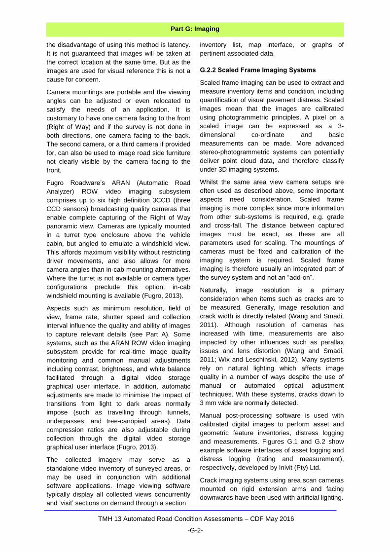
Manual post-processing software is used with
calibrated digital images to perform asset and
geometric feature inventories, distress logging
and measurements. Figures G.1 and G.2 show
example software interfaces of asset logging and
distress logging (rating and measurement),
respectively, developed by Inivit (Pty) Ltd.
Crack imaging systems using area scan cameras
mounted on rigid extension arms and facing
downwards have been used with artificial lighting.
TMH 13 Automated Road Condition Assessments – CDF May 2016
-G-3-
Part G: Imaging
Figure G.1 Asset logging and condition rating interface (Inivit, 2010)
Figure G.2 Pavement distress logging and measurement interface (Inivit, 2010)
Fugro’s Pave2D system uses two high resolution
monochrome digital cameras triggered by a DMI
to capture a continuous stream of pavement
imagery over the full lane width. High camera
resolution (1392 x 1040 pixels), a synchronized
high speed shutter setting in combination with
optimally angled camera-synchronised strobe
lights enable recognition of cracks down to
2 mm wide. Strobe lights eliminate shadows from
trees, bridges and other objects providing
consistent illumination of pavement images.
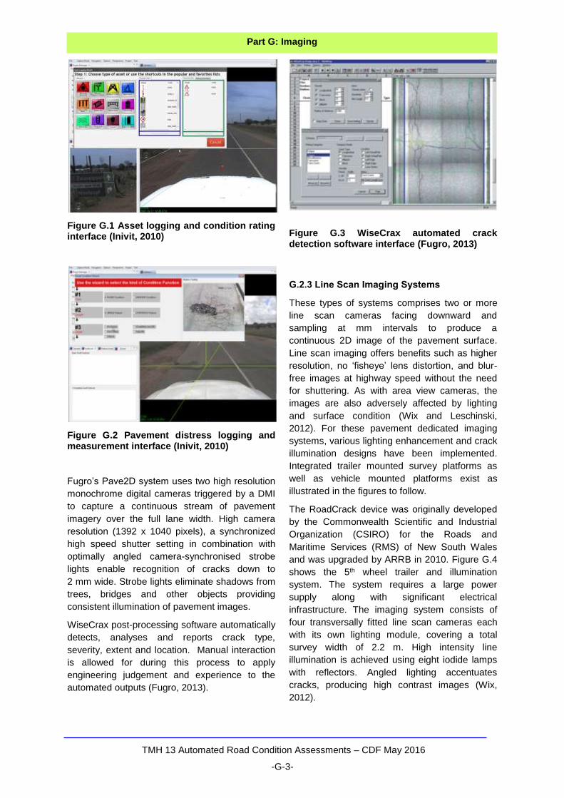
WiseCrax post-processing software automatically
detects, analyses and reports crack type,
severity, extent and location. Manual interaction
is allowed for during this process to apply
engineering judgement and experience to the
automated outputs (Fugro, 2013).
Figure G.3 WiseCrax automated crack detection software interface (Fugro, 2013)
G.2.3 Line Scan Imaging Systems
These types of systems comprises two or more
line scan cameras facing downward and
sampling at mm intervals to produce a
continuous 2D image of the pavement surface.
Line scan imaging offers benefits such as higher
resolution, no ‘fisheye’ lens distortion, and blur-
free images at highway speed without the need
for shuttering. As with area view cameras, the
images are also adversely affected by lighting
and surface condition (Wix and Leschinski,
2012). For these pavement dedicated imaging
systems, various lighting enhancement and crack
illumination designs have been implemented.
Integrated trailer mounted survey platforms as
well as vehicle mounted platforms exist as
illustrated in the figures to follow.
The RoadCrack device was originally developed
by the Commonwealth Scientific and Industrial
Organization (CSIRO) for the Roads and
Maritime Services (RMS) of New South Wales
and was upgraded by ARRB in 2010. Figure G.4
shows the 5th wheel trailer and illumination
system. The system requires a large power
supply along with significant electrical
infrastructure. The imaging system consists of
four transversally fitted line scan cameras each
with its own lighting module, covering a total
survey width of 2.2 m. High intensity line
illumination is achieved using eight iodide lamps
with reflectors. Angled lighting accentuates
cracks, producing high contrast images (Wix,
2012).

TMH 13 Automated Road Condition Assessments – CDF May 2016
-G-4-
Part G: Imaging
Automated crack detection and analysis is
performed in real time without the need for post
processing or data handling.
Processing of results include crack classification
and crack width measurement down to 1 mm. All
images, or optionally only those containing
cracks, can be saved in compressed or
uncompressed format (Wix and Leschinski,
2012).
Figure G.4 RoadCrack trailer and pavement lighting (Wix and Leschinski, 2012)
INO Systems in collaboration with PavemetricsTM
Systems Inc. developed the Laser Road Imaging
System (LRIS). The LRIS represents a data
acquisition system that uses two line scan
cameras in conjunction with laser line projectors
that are aligned in the same plane in a
symmetrically crossed optical configuration.
As shown in Figure G.5, this optical configuration
increases the visibility of cracks by using the
incident illumination angle of the line laser to
cause the cracks to project shadows. The LRIS
system can operate in full daylight as well as in
darkness because it is immune to variations in
outside lighting conditions and unwanted
shadows. The system only consumes a few
hundred watts of power compared to more
traditional lighting systems. The system images
near 4 meter transverse road sections at more
than 100km/h with 1 mm resolution.
Figure G.5 Laser Road Imaging System (Pavemetrics, 2010)
The LRIS has been implemented by service
providers such as Dynatest (Figure G.6).
Dynatest’s post-processing software is used for
manual distress identification, measurement, and
classification.
Figure G.6 Dynatest Multi-Functional Vehicle
G.2.4 Range Imaging Systems
As described in Part A, range imaging produces
a 3D structure of a scene employing active range
sensors consisting of a light source and receiver.
The most commonly used systems use laser line
projectors and high speed cameras, respectively.
High speed CCD or CMOS cameras detect the
changes in the laser line or light strip. By using
optical triangulation, a depth map of surface
points under the strip is obtained. High speed
cameras typically generate a couple of thousand
profiles per second while scanning an object
which is used to construct the 3D image. With
these sensors, the application range is normally
from millimetres to a few meters, whilst sub-
millimetre resolutions can be achieved.
TMH 13 Automated Road Condition Assessments – CDF May 2016
-G-5-
Part G: Imaging
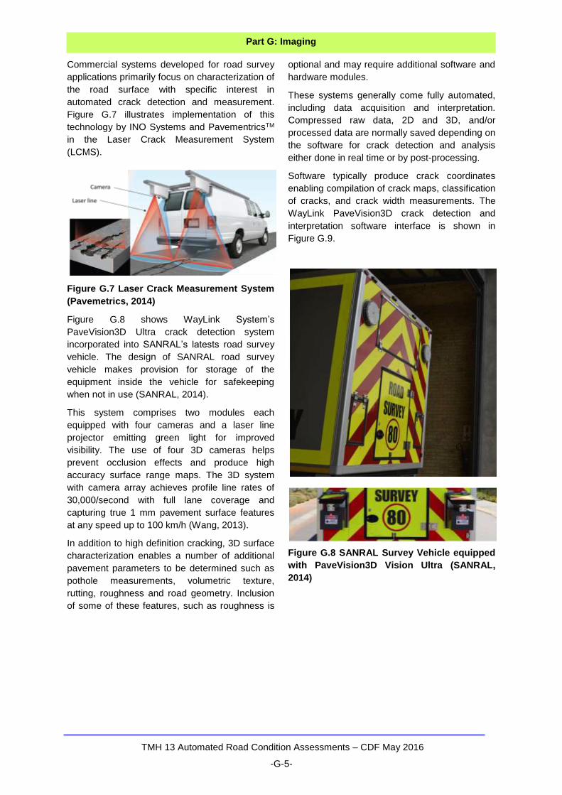
Commercial systems developed for road survey
applications primarily focus on characterization of
the road surface with specific interest in
automated crack detection and measurement.
Figure G.7 illustrates implementation of this
technology by INO Systems and PavementricsTM
in the Laser Crack Measurement System
(LCMS).
Figure G.7 Laser Crack Measurement System
(Pavemetrics, 2014)
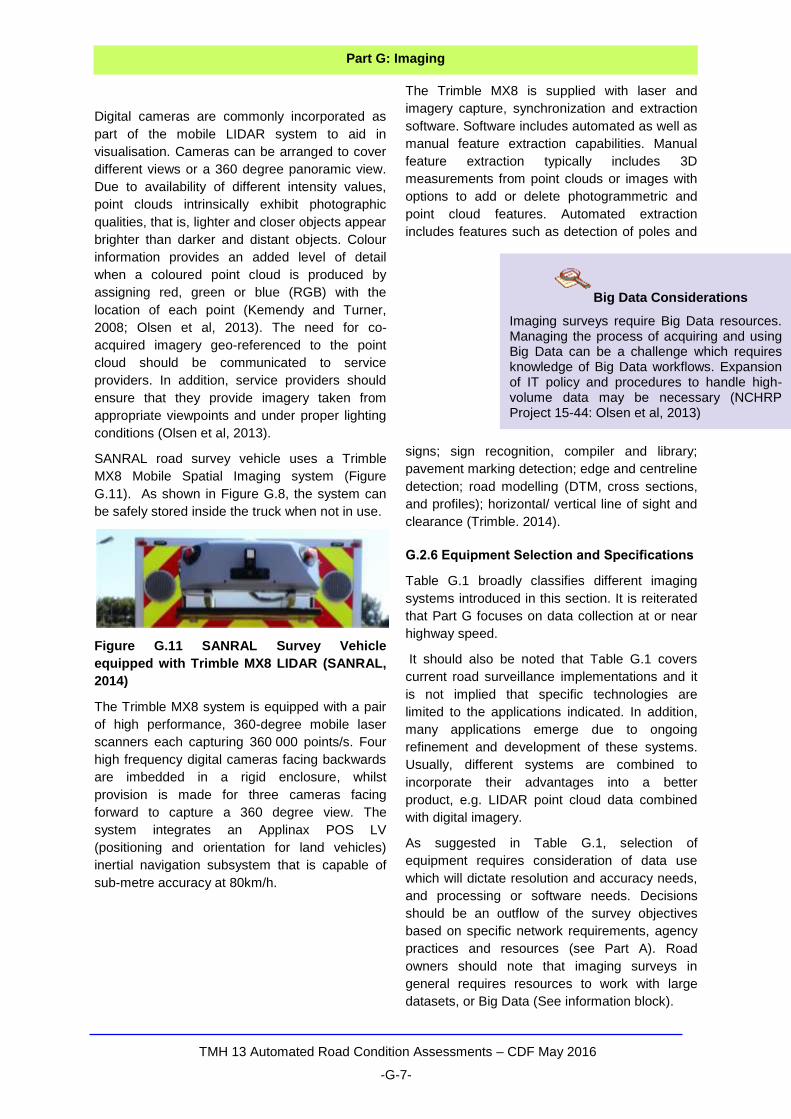
Figure G.8 shows WayLink System’s
PaveVision3D Ultra crack detection system
incorporated into SANRAL’s latests road survey
vehicle. The design of SANRAL road survey
vehicle makes provision for storage of the
equipment inside the vehicle for safekeeping
when not in use (SANRAL, 2014).
This system comprises two modules each
equipped with four cameras and a laser line
projector emitting green light for improved
visibility. The use of four 3D cameras helps
prevent occlusion effects and produce high
accuracy surface range maps. The 3D system
with camera array achieves profile line rates of
30,000/second with full lane coverage and
capturing true 1 mm pavement surface features
at any speed up to 100 km/h (Wang, 2013).
In addition to high definition cracking, 3D surface
characterization enables a number of additional
pavement parameters to be determined such as
pothole measurements, volumetric texture,
rutting, roughness and road geometry. Inclusion
of some of these features, such as roughness is
optional and may require additional software and
hardware modules.
These systems generally come fully automated,
including data acquisition and interpretation.
Compressed raw data, 2D and 3D, and/or
processed data are normally saved depending on
the software for crack detection and analysis
either done in real time or by post-processing.
Software typically produce crack coordinates
enabling compilation of crack maps, classification
of cracks, and crack width measurements. The
WayLink PaveVision3D crack detection and
interpretation software interface is shown in
Figure G.9.
Figure G.8 SANRAL Survey Vehicle equipped
with PaveVision3D Vision Ultra (SANRAL,
2014)

TMH 13 Automated Road Condition Assessments – CDF May 2016
-G-6-
Part G: Imaging
Figure G.9 PaveVision3D Ultra crack detection and analysis interface (Wang, 2013)
G.2.5 Three-dimensional (3D) Laser Scanning
3D laser scanning or LIDAR (Light Detection and
Ranging) can rapidly acquire a substantial
amount of highly detailed geospatial information.
The value of this technology is in the features of
the road and road side inventory that can be
extracted from the data such as bridge clearance,
gantry locations, sight distance, curvature,
barriers etc. Whilst this technology has
successfully been used to measure pavement
rutting and roughness, its application to
automated distress detection largely remains in
the research and development arena (Olsen et
al, 2013).
Laser scanners work by emitting light and
detecting the reflected light from an object to
accurately determine the distance to that object.
3D laser scanners facilitate millions of
measurements in a few seconds through firing
laser pulses either by an internal rotating mirror
(fixed scanning head) or rotating scanning head
operation (Olsen et al, 2013). Immediately after
one pulse is received and measured, the scanner
transmits another pulse at a fixed angular
increment. The distance and orientation of each
pulse allows determination of the associated xyz
coordinates. In addition, the intensity (signal
strength) of the reflected pulse is determined. In
general, higher reflections are associated with
lighter coloured objects and closer objects. The
coordinates and intensity values output of
millions of measurements make up the ‘point
cloud’ (Kemendy and Turner, 2008).
The accuracy of the positioning system of the
mobile LIDAR largely determines the accuracy of
the final point cloud. Measurements from all
system components are synchronized to a
common time reference frame using a precise
time stamp. Figure G.10 shows typical
components of a mobile LIDAR system. Refer to
TMH13 Parts A and B for further information on
positioning systems.
A rigid platform is needed to firmly attach the
laser scanners, positioning components, digital
cameras and ancillary devices. Careful
calibration of each component is required so that
the offsets between them are known and remain
stable. In addition, the platform may be designed
in such a way to make provision for transfer of
the mobile LIDAR system from vehicle-to-vehicle
with more ease than moving individual
components (Olsen et al, 2013).
Figure G.10 Typical mobile LIDAR components (Olsen et al, 2013)
TMH 13 Automated Road Condition Assessments – CDF May 2016
-G-7-
Part G: Imaging
Digital cameras are commonly incorporated as
part of the mobile LIDAR system to aid in
visualisation. Cameras can be arranged to cover
different views or a 360 degree panoramic view.
Due to availability of different intensity values,
point clouds intrinsically exhibit photographic
qualities, that is, lighter and closer objects appear
brighter than darker and distant objects. Colour
information provides an added level of detail
when a coloured point cloud is produced by
assigning red, green or blue (RGB) with the
location of each point (Kemendy and Turner,
2008; Olsen et al, 2013). The need for co-
acquired imagery geo-referenced to the point
cloud should be communicated to service
providers. In addition, service providers should
ensure that they provide imagery taken from
appropriate viewpoints and under proper lighting
conditions (Olsen et al, 2013).
SANRAL road survey vehicle uses a Trimble
MX8 Mobile Spatial Imaging system (Figure
G.11). As shown in Figure G.8, the system can
be safely stored inside the truck when not in use.
Figure G.11 SANRAL Survey Vehicle
equipped with Trimble MX8 LIDAR (SANRAL,
2014)
The Trimble MX8 system is equipped with a pair
of high performance, 360-degree mobile laser
scanners each capturing 360 000 points/s. Four
high frequency digital cameras facing backwards
are imbedded in a rigid enclosure, whilst
provision is made for three cameras facing
forward to capture a 360 degree view. The
system integrates an Applinax POS LV
(positioning and orientation for land vehicles)
inertial navigation subsystem that is capable of
sub-metre accuracy at 80km/h.
The Trimble MX8 is supplied with laser and
imagery capture, synchronization and extraction
software. Software includes automated as well as
manual feature extraction capabilities. Manual
feature extraction typically includes 3D
measurements from point clouds or images with
options to add or delete photogrammetric and
point cloud features. Automated extraction
includes features such as detection of poles and
signs; sign recognition, compiler and library;
pavement marking detection; edge and centreline
detection; road modelling (DTM, cross sections,
and profiles); horizontal/ vertical line of sight and
clearance (Trimble. 2014).
G.2.6 Equipment Selection and Specifications
Table G.1 broadly classifies different imaging
systems introduced in this section. It is reiterated
that Part G focuses on data collection at or near
highway speed.
It should also be noted that Table G.1 covers
current road surveillance implementations and it
is not implied that specific technologies are
limited to the applications indicated. In addition,
many applications emerge due to ongoing
refinement and development of these systems.
Usually, different systems are combined to
incorporate their advantages into a better
product, e.g. LIDAR point cloud data combined
with digital imagery.
As suggested in Table G.1, selection of
equipment requires consideration of data use
which will dictate resolution and accuracy needs,
and processing or software needs. Decisions
should be an outflow of the survey objectives
based on specific network requirements, agency
practices and resources (see Part A). Road
owners should note that imaging surveys in
general requires resources to work with large
datasets, or Big Data (See information block).
Big Data Considerations
Imaging surveys require Big Data resources. Managing the process of acquiring and using Big Data can be a challenge which requires knowledge of Big Data workflows. Expansion of IT policy and procedures to handle high-volume data may be necessary (NCHRP Project 15-44: Olsen et al, 2013)
TMH 13 Automated Road Condition Assessments – CDF May 2016
-G-8-
Part G: Imaging
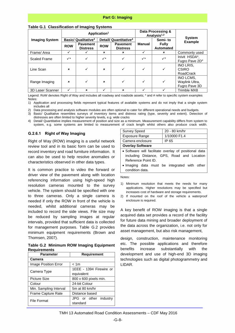
Table G.1 Classification of Imaging Systems
Imaging System
Application1 Data Processing &
Analysis1,2 System
Example Basic/ Qualitative3 Detail/ Quantitative4
Manual Semi- to
Fully Automated
ROW Pavement Distress
ROW Pavement Distress
Frame/ Area Commonly used
Scaled Frame * * * #
Inivit HSDA*, Fugro Pave 2D#
Line Scan INO LRIS, CSIRO RoadCrack
Range Imaging INO LCMS, Waylink Ultra, Fugro Pave 3D
3D Laser Scanner Trimble MX8
Legend: RoW denotes Right of Way and includes all roadway and roadside assets; * and # refer to specific system examples Notes: 1) Application and processing fields represent typical features of available systems and do not imply that a single system
includes all 2) Data processing and analysis software modules are often optional to cater for different operational needs and budgets. 3) Basic/ Qualitative resembles surveys of inventory items and distress rating (type, severity and extent). Detection of
distresses are often limited to higher severity levels, e.g. wide cracks 4) Detail/ Quantitative implies measurement of position and size as a minimum. Measurement capability differs from system to
system, e.g. some systems are limited to measurement of crack length whilst others also produce crack width.
G.2.6.1 Right of Way Imaging
Right of Way (ROW) imaging is a useful network
review tool and in its basic form can be used to
record inventory and road furniture information. It
can also be used to help resolve anomalies or
characteristics observed in other data types.
It is common practice to video the forward or
driver view of the pavement along with location
referencing information using high-speed high
resolution cameras mounted to the survey
vehicle. The system should be specified with one
to three cameras. Only a single camera is
needed if only the ROW in front of the vehicle is
needed, whilst additional cameras may be
included to record the side views. File size may
be reduced by sampling images at regular
intervals, provided that sufficient data is collected
for management purposes. Table G.2 provides
minimum equipment requirements (Brown and
Thomsen, 2007).
Table G.2 Minimum ROW Imaging Equipment Requirements
Parameter Requirement
Camera
Image Position Error < 1m
Camera Type 1EEE - 1394 Firewire or
equivalent
Picture Size 800 x 600 pixels min.
Colour 24-bit Colour
Min. Sampling Interval 5m at 80 km/hr
Frame Capture Rate Distance based
File Format JPG or other industry
standard
Survey Speed 20 - 80 km/hr
Exposure Range 1/10000 F1.4
Camera enclosure IP 65
Overlay Software
Software will facilitate overlay of positional data
including Distance, GPS, Road and Location
Reference Point ID.
Imaging data must be integrated with other
condition data.
Notes:
1) Minimum resolution that meets the needs for many
applications. Higher resolutions may be specified but
increases cost of hardware and storage requirements.
2) If mounted on the roof of the vehicle a waterproof
enclosure is required.
A key benefit of ROW imaging is that a single
acquired data set provides a record of the facility
for future data mining and broader deployment of
the data across the organization, i.e. not only for
asset management, but also risk management,
design, construction, maintenance monitoring
etc. The possible applications and therefore
benefits increase substantially with the
development and use of high-end 3D imaging
technologies such as digital photogrammetry and
LIDAR.
TMH 13 Automated Road Condition Assessments – CDF May 2016
-G-9-
Part G: Imaging
Much emphasis has been placed on the use of
mobile LIDAR in the transportation sector in
recent years (Faber, 2014). However, modern
photogrammetry offers a competitive alternative
in meeting specifications for infrastructure
mapping. Traditionally the equipment cost for
photogrammetric systems are significantly less if
compared to LIDAR although considerable cost
reductions are expected with advances in LIDAR
technology (Nulty and Noble, 2013). In many
cases, these technologies are often (and ideally)
integrated and used in a complementary fashion.
In the context of TMH 13 it is assumed that most
agencies will hire the services of contractors for
data collection and processing. As accuracy
requirements for 3D imaging are increased, the
survey cost can increase exponentially. These
costs are associated for example with the
establishment of a very accurate survey control
framework, increased number of ground control
targets, number of phases in each direction, the
use of high grade IMU and scanner(s) and
additional office processing (Faber, 2014). Apart
from data collection costs and information
technology (IT) costs (storage, servers, backups
etc.) consideration should be given to data
extraction costs. These costs rely heavily on the
number of features to be extracted and the level
of automation of this process. Manual
identification and extraction of features can be
labour intensive. Depending on the feature, even
systems with highly automated feature extraction
capabilities generally exhibit accuracies of about
80 percent. Cost-effective extraction of data is
therefore critical to realising the benefit of 3D
imaging (Faber et al, 2014).
Although using a technology such as mobile
LIDAR has many benefits, it may not always be
the optimal solution for the network under
consideration. The significant volumes of data
generated by 3D imaging systems provide a
valuable, yet challenging resource (See
information block on ‘Big Data Considerations’). It
should be noted that the agency may be more
concerned with the end product than the
technique used to collect the data. A cost/benefit
analysis should be conducted to determine if the
candidate technique is optimal for the survey
under consideration especially when considering
high-end solutions such as mobile LIDAR. Such
an analysis should consider (Olsen et al, 2013):
All potential data uses during data life span;
Capacity needed to perform quality control;
Integration of data into current workflows and
possible improvements to current systems;
The ability to share data and cost within and
outside the agency;
Survey resolution and accuracy needs, and
Collection of additional data from the same
platform.
Specifications for 3D imaging surveys generally
address the required information and data quality
that should be provided and are broad enough
not to limit service provider equipment and
technology. Although detailed equipment
component specifications are not required, the
agency may specify the equipment type
depending on aspects such as past experience,
survey objectives, network characteristics and
agency resources that should reflect in the
cost/benefit analysis. Because accuracies of
equipment components and system parameters
impact the overall expected data accuracies, an
equipment calibration report should be requested
from the service provider as part of the validation
process (See Section G.3).
Different data applications require different levels
of accuracy and density (resolution) of data. Data
quality requirements will dictate the use of
equipment or service providers with appropriate
capabilities. For this reason the level of detail or
general data application category needs to be
established for data collection procurement
purposes.

TMH 13 Automated Road Condition Assessments – CDF May 2016
-G-10-
Part G: Imaging
A mobile LIDAR application matrix developed
under NCHRP Project 15-44 (Olsen et al, 2013)
offers suggested accuracy and resolution
requirements for different applications (Appendix
G-1). This matrix may be used as an indication of
the desired output for any equipment capable of
producing a point cloud dataset. The matrix in
Appendix G-1 presents nine categories (1A
through 3C) where the numbers represent
varying orders of accuracy (1 = High, 2 =
Medium, 3 = Low) and letters representing levels
of point density on the targets of interest (A =
Coarse, B = Intermediate, C = Fine).
Accuracy has the greatest influence on project
cost whilst point density can be achieved by
driving slower or making multiple passes. As an
example, for asset management and inventory
mapping applications the matrix recommends
Category 3C: Intermediate Density (30 to 100
points/m2) and Low Accuracy (>0.2 m). However,
when determining appropriate requirements for
procurement purposes, specific project
requirements and agency practices also need to
be considered.
Ideally, an agency would coordinate needs
between departments to determine optimum data
utilisation. Naturally, datasets collected at higher
accuracies and point densities (e.g. Category 1A)
will be usable for applications that require lower
quality data (e.g. Category 2B), although this may
not be cost-effective. In contrast, data collected
at a lower accuracy and point density (e.g.
Category 2B) may still be useful for an
application requiring higher quality data (e.g.
Category 1A) compared to what is available.
However, the analysis may be more difficult to
perform and less reliable than if the
recommended higher category data were
collected (Olsen et al, 2013). Once the network
manager has decided on the general data
collection category, detailed contract
requirements can be developed. More detailed
aspects are included in Section G.3.
G.2.6.2 Pavement Distress Imaging
Typical distress imaging systems introduced,
highlight a general focus on crack detection and
analysis. The systems typically capture pavement
images using a high-speed-high-resolution
camera mounted securely to the survey vehicle
such that the pavement surface detail is recorded
along with location reference information.
The recording method may be area scanning,
line scanning, or 3D scanning. Systems with
illumination or without (passive) can be used.
Images may be recorded as a dimensional map
or any combination of technologies that achieves
the specified distress rating or crack detection
reliability.
Table G.3 provides minimum equipment
requirements. Whilst basic equipment
specifications are presented, acceptance is
primarily based on adequate validation to meet
specified system output criteria (see Section
G.3). Specifications should aim to standardize
thereby contributing to consistent pavement
condition estimates while not unduly limiting
equipment innovation (AASHTO, 2014a).
Table G.4 classifies pavement distress imaging
systems into two classes based on typical system
capabilities. Detailed crack analysis can be done
with Class 1 systems, whilst Class 2 systems are
essentially used for distress ratings. The
classification also considers processing. For
semi-automated processing, software facilitates
recording and detailed measurement of
distresses by the reviewer, whilst automated
systems detect, record, and analyse distresses,
often refined with human intervention. With
manual processing, the reviewer uses software to
view the images, while assigning and recording
types of distresses and condition ratings.
Compared to manual (or traditional) reference
methods as described in TMH 9, higher level of
automation in the methodology offers benefits in
improved personnel safety, more rapid and cost
effective data collection, better reporting and
planning capabilities, production of higher quality
data in terms of repeatability, and potentially
better statistical representation of the network
(Austroads, 2006). As indicated above and
similar to high-end ROW imaging technologies,
the selection/ specification of distress imaging
equipment involves big data considerations, i.e.
More Information: Selecting and Implementing Mobile LIDAR Technology
NCHRP Project 15-44 “Guidelines for the Use of Mobile LIDAR in Transportation Applications” (Olsen et al, 2013) provides information on aspects such as workflow and data management, organizational data mining, procurement considerations, and implementation plans for transportation agencies
TMH 13 Automated Road Condition Assessments – CDF May 2016
-G-11-
Part G: Imaging
Table G.3 Minimum Equipment Specifications for Distress Imaging
Parameter Requirement
Camera
Image Position Error < 1m
Camera Type Area or line scan
Colour 8-bit grey scale
Minimum resolution 2mm/pixel
File Format JPG or other industry
standard
Minimum coverage 100% of lane width
+ 300 mm
Maximum image length
in travel direction 100 m
Survey Speed 20 - 80 km/hr
Camera enclosure IP 65
Review Software
Software will facilitate on demand viewing and full
logging and condition rating to produce an inventory
of pavement defects that can be integrated with
other condition data.
the ability of the agency to utilise and effectively
manage the data. The type of network, agency
objectives and resources need to be taken into
account. The following general considerations
affect the selection and specification of
equipment (adapted from Austroads, 2006):
Data collected and processed using fully
automated systems may be more expensive
due to higher equipment cost. However, time
and reliability of processing should be
considered for systems that rely on manual
distress detection, analysis and rating.
Detailed reporting is possible with automated
distress detection and processing, including
crack type, crack width, severity, and extent.
Systems that can detect more detail,
potentially offer higher savings through
correctly targeted early application of low cost
maintenance treatments.
More dedicated systems normally has less
restrictions such as the ability to conduct
surveys during daylight (irrespective of
position of sun) or at night.
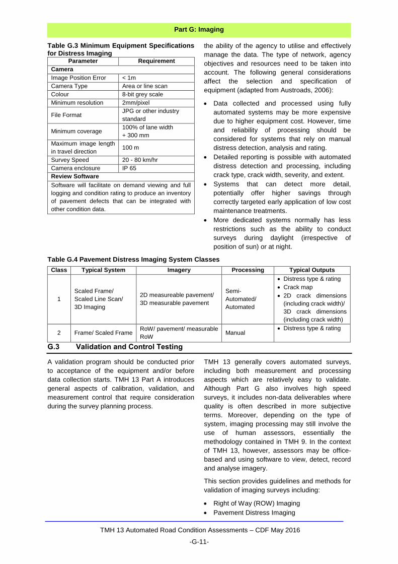
Table G.4 Pavement Distress Imaging System Classes
G.3 Validation and Control Testing
A validation program should be conducted prior
to acceptance of the equipment and/or before
data collection starts. TMH 13 Part A introduces
general aspects of calibration, validation, and
measurement control that require consideration
during the survey planning process.
TMH 13 generally covers automated surveys,
including both measurement and processing
aspects which are relatively easy to validate.
Although Part G also involves high speed
surveys, it includes non-data deliverables where
quality is often described in more subjective
terms. Moreover, depending on the type of
system, imaging processing may still involve the
use of human assessors, essentially the
methodology contained in TMH 9. In the context
of TMH 13, however, assessors may be office-
based and using software to view, detect, record
and analyse imagery.
This section provides guidelines and methods for
validation of imaging surveys including:
Right of Way (ROW) Imaging
Pavement Distress Imaging
Class Typical System Imagery Processing Typical Outputs
1
Scaled Frame/
Scaled Line Scan/
3D Imaging
2D measureable pavement/
3D measurable pavement
Semi-
Automated/
Automated
Distress type & rating
Crack map
2D crack dimensions
(including crack width)/
3D crack dimensions
(including crack width)
2 Frame/ Scaled Frame RoW/ pavement/ measurable
RoW Manual
Distress type & rating
TMH 13 Automated Road Condition Assessments – CDF May 2016
-G-12-
Part G: Imaging
G.3.1 General Approach
Calibration and validation concepts are
introduced in Part A. Part A describes validation
as a referencing exercise conducted on
predetermined validation (or reference) sections.
The survey system must be validated at each of
the selected validation sites against reference
data. Reference surveys are conducted by the
agency (or third party) using appropriate
reference survey techniques.
Calibration and validation are required before
production data collection starts and include
aspects such as personnel training/ calibration/
certification, equipment calibration/ certification,
selection of validation sites or points, performing
reference and validation surveys, and application
of validation criteria. Once the system has been
accepted and production surveys start, control
testing should be done on a regular basis to
ensure that the system remains valid throughout
the survey contract.
G.3.2 Calibration
Components of equipment are configured
according to the purchaser’s requirements and
calibrated as specified by the manufacturer.
Some of these components can only be
calibrated by the manufacturer while other
aspects of the system can be calibrated by the
owner. Where imaging outputs are used for
measurement, such as in photogrammetric,
LIDAR, and pavement distress measurement
systems, a rigid framework is normally used to
firmly attach the scanners, cameras, positioning
components, and ancillary devices. However,
depending on the system and the methodology
used to install the components, the system
calibration parameters may not be of a high
temporal stability. Providers are therefore
required to submit a calibration report that
contains the following minimum information
(Olsen et al, 2013):
The equipment used for data collection;
Equipment installation schematics;
The calibration procedure used;
The calibration parameters and estimated
accuracies, and
Verification of temporal or long term stability
of calibrated parameters
For visual assessments or distress ratings
required as part of manual or semi-automated
image processing, validation sites are used to
train and calibrate assessors in the proper
application of the THM 9 or specified protocols.
For fully automated processes, validation sites
are used to calibrate and adjust software
algorithms that are used for data reduction.
Compatibility of outputs with TMH 9, TMH 20,
and TMH 22 is required. Appendix G-2 provides
definitions of distresses, in particular cracks, to
complement TMH 9 for interpretation from an
image analysis software perspective. More
detailed methodologies are provided
subsequently in sections that deal with validation.
G.3.3 Validation Test Requirements
Part A includes general guidance for the
selection of validation sections. This part outlines
additional requirements and considerations for
the selection of sections or sites for imaging
validation. Concepts of geometric correction and
validation required for 3D imaging (such as
LIDAR that produces point cloud data) are
different from general imaging and these aspects
are therefore presented separately.
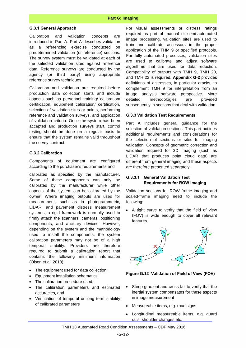
G.3.3.1 General Validation Test
Requirements for ROW Imaging
Validation sections for ROW frame imaging and
scaled-frame imaging need to include the
following:
A tight curve to verify that the field of view
(FOV) is wide enough to cover all relevant
features.
Figure G.12 Validation of Field of View (FOV)
Steep gradient and cross-fall to verify that the
inertial system compensates for these aspects
in image measurement
Measureable items, e.g. road signs
Longitudinal measureable items, e.g. guard
rails, shoulder changes etc.
TMH 13 Automated Road Condition Assessments – CDF May 2016
-G-13-
Part G: Imaging
Areas with ambient light changes i.e. trees
next to the road to verify that the camera(s)
compensates for changes in ambient light
It should be noted that the requirements outlined
above are different from normal straight or
tangent sections recommended for validation of
other pavement surveillance measurements.
These sites may therefore not be appropriate to
use for validation of other equipment.
A minimum of five (5) validation sections shall be
selected each with a length of one (1) kilometre.
Each site shall have a lead-in and lead-out of at
least 0.1 km to visually assist validation of start
and end locations.
No validation data shall be collected if the
surveillance vehicle is forced to collect the
majority of the data while travelling towards the
sun. Validation sections should not have excess
water on the roadway nor should any validation
imaging occur during inclement weather. ROW
imaging shall only be performed during daytime
hours under sufficient ambient lighting conditions.
The reference or benchmark data for general
ROW imaging is an inventory of visible items for
each section, with unique item identifier, and
location reference. Where item dimension
measurement is required, the items with relevant
dimensions, geo-references and other location
referencing that apply should be included.
G.3.3.2 Control and Validation Points for 3D
ROW Imaging
Three dimensional (3D) ROW Imaging generally
refers to any system capable of producing a point
cloud dataset, whether obtained from laser
scanning (e.g. LIDAR) or 3D reconstruction (high-
end photogrammetric systems). In addition to
general requirements for validating ROW
imaging, aspects addressed in the following
paragraphs shall apply.
Point cloud data, especially at high accuracy
levels, will generally not meet engineering survey
standards without geometric correction to
benchmark control points (or local transformation
points). These control points are identified in the
imagery and the point cloud is adjusted by a local
transformation to the well defined control point
locations. Validation points are independent from
control points and used as a reference to verify
the final geospatial values (Olsen et al, 2013;
Faber, 2014).
Depending on the point cloud accuracy level
specified (Section G.3.4) required accuracies
may be achieved without geometric adjustment
by combining data from multiple runs, collected
by systems equipped with high accuracy inertial
measurement units (IMUs). Although setting up
control points may be redundant in such cases,
validation points are still needed to verify system
accuracy (Faber, 2014).
Datasets shall be tested with a minimum of 20
validation points. Based on NCHRP Project
14-55 (Olsen et al, 2013) control and validation
points:
Can either be established as part of a
permanent control network or can be project
specific and temporary.
Shall be located at the beginning, end, and
widely distributed throughout the project
corridor to reflect variance across the project
extents.
Can be artificial or existing natural targets that
have been appropriately surveyed with an
independent source.
In selecting the characteristics and placement of
targets, consideration shall be given to:
Appropriate size relative to point cloud
resolution.
Shapes suitable to allow both vertical and
horizontal accuracy validation.
Use of non-reflective and reflective targets.
Potential issues with reflective targets
surveyed using laser scanners.
Safe placement as close as possible to the
survey vehicle path.
Important!
Where high accuracy levels warrant geometric correction of the point cloud, the control points observed in the dataset shall serve as direct input observations into the raw navigation trajectory estimation during post-processing, i.e. Geometric correction shall be applied though re-processing of system navigation trajectory. Full documentation including methodology, type, and magnitudes of any applied geometric correction should be provided (NCHRP Project 15-44: Olsen et al, 2013)
TMH 13 Automated Road Condition Assessments – CDF May 2016
-G-14-
Part G: Imaging
Placement on both sides of the road, across
or alternately.
Placement on other features of interest, where
the road is not the only or primary data of
interest.
Table G.5 provides control point spacing and
intervals for selection of validation point spacing,
depending on the required accuracy. Point
density validation shall also be conducted
throughout the dataset using similar intervals,
particularly for objects of interest. The frequency
of validation needs to be established and
depends on the variability observed in the
dataset as well as spatial frequency of the
objects of interest (Olsen et al, 2013).
Control and validation point datasets shall be of a
higher accuracy than the point cloud accuracy
specifications. Reference datasets shall be
obtained independently through DGPS or total
station surveying. As an example (refer to
Section G.2.6.1 and Appendix G-1), for accuracy
level 1 certification, static GPS surveying would
be required. For accuracy levels 2 and 3
certification, faster methods such as RTK GPS
can generally be used (Olsen et al, 2013).
Table G.5 Control and Validation point Intervals for different Accuracy Levels
Accuracy
Level1
Control Point
Interval2
Validation Point
Interval
1 ≤ 450 m 150 - 300 m
2 ≤ 450 m* 300 - 750 m
3 ≤ 450 m* 750 - 1500 m
Notes:
1) Refer to Section G.2.6.1 and Appendix G-1 2) Control points may not be required for lower accuracy
levels*
G.3.3.3 Validation Test Requirements for
Pavement Distress Imaging
In order to validate the performance of pavement
distress imaging systems, especially in avoiding
the reporting of false positive cracks, a variety of
sections should include features such as (PIARC,
2012):
Representative crack types;
Sealed cracks;
Different surface types, textures in particular;
Bleeding and aggregate loss;
Patches and potholes;
Road markings;
Bridge joints, grid inlets etc. and
Longitudinal and transverse joints where
concrete pavements form part of the network.
No data shall be collected during inclement
weather or under wet pavement conditions.
Although systems equipped with artificial
illumination may be able to collect data at night,
basic ROW imaging may still be required. Care
shall be taken to ascertain sufficient lighting
conditions for all surveys at all times.
Table G6 summarises validation test
requirements for pavement distress imaging
systems. General requirements are provided as
well as specific requirements for Class 1
systems, i.e. with semi-automated and
automated processing capabilities. For Class 1
systems, the collection lane is divided into five
strips or zones to complement the analysis
process. Whilst default widths are provided for
Zones 2, 3, and 4 (inside, between, and outside
wheel paths, respectively), Zones 1 and 5 will
vary depending on the lane width under
consideration.
Validation of Class 1 systems is divided into two
parts: The ability of the system to detect cracks
and secondly, the ability to properly analyse the
cracks or crack map. To validate system
detection capability, actual field measurements
(and not measurements from images) shall be
used as a reference. Whilst THM 9 field distress
ratings are not required in this part of the method,
compilation of a database with this level of
ground truth data can be utilised effectively to
continually improve confidence in these systems
by scrutinizing, calibrating, and developing
distress analysis algorithms.
TMH 13 Automated Road Condition Assessments – CDF May 2016
-G-15-
Part G: Imaging
Validation of the Class 1 system analysis
capability uses imagery collected for the
validation sections as the reference data set. The
primary data obtained during this process are
software facilitated detail distress dimension
measurements and mapping. TMH 9 visual
ratings shall also be reported for relevant
distresses typically detectable by automated
systems as outlined in Appendix G-2. In
addition, the full record of relevant visual surface
data and distresses as defined in TMH 9 shall be
recorded. The latter may require supplemental
manual reviews and recording of distresses that
are not automatically detected.
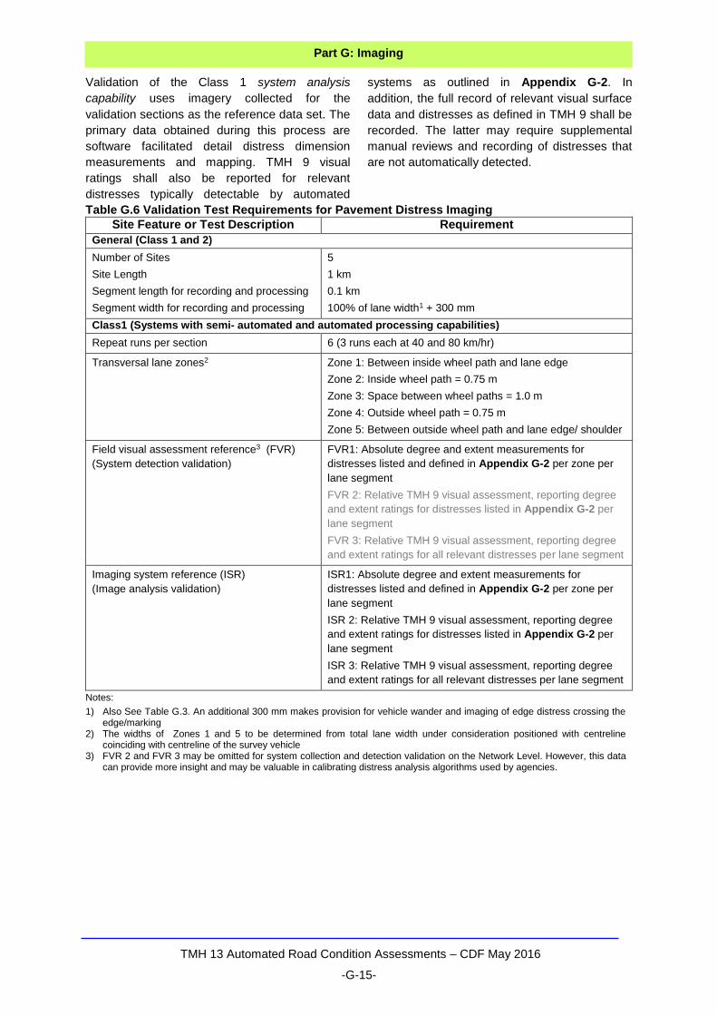
Table G.6 Validation Test Requirements for Pavement Distress Imaging
Site Feature or Test Description Requirement
General (Class 1 and 2)
Number of Sites
Site Length
Segment length for recording and processing
Segment width for recording and processing
5
1 km
0.1 km
100% of lane width1 + 300 mm
Class1 (Systems with semi- automated and automated processing capabilities)
Repeat runs per section 6 (3 runs each at 40 and 80 km/hr)
Transversal lane zones2 Zone 1: Between inside wheel path and lane edge
Zone 2: Inside wheel path = 0.75 m
Zone 3: Space between wheel paths = 1.0 m
Zone 4: Outside wheel path = 0.75 m
Zone 5: Between outside wheel path and lane edge/ shoulder
Field visual assessment reference3 (FVR)
(System detection validation)
FVR1: Absolute degree and extent measurements for
distresses listed and defined in Appendix G-2 per zone per
lane segment
FVR 2: Relative TMH 9 visual assessment, reporting degree
and extent ratings for distresses listed in Appendix G-2 per
lane segment
FVR 3: Relative TMH 9 visual assessment, reporting degree
and extent ratings for all relevant distresses per lane segment
Imaging system reference (ISR)
(Image analysis validation)
ISR1: Absolute degree and extent measurements for
distresses listed and defined in Appendix G-2 per zone per
lane segment
ISR 2: Relative TMH 9 visual assessment, reporting degree
and extent ratings for distresses listed in Appendix G-2 per
lane segment
ISR 3: Relative TMH 9 visual assessment, reporting degree
and extent ratings for all relevant distresses per lane segment
Notes:
1) Also See Table G.3. An additional 300 mm makes provision for vehicle wander and imaging of edge distress crossing the edge/marking
2) The widths of Zones 1 and 5 to be determined from total lane width under consideration positioned with centreline coinciding with centreline of the survey vehicle
3) FVR 2 and FVR 3 may be omitted for system collection and detection validation on the Network Level. However, this data can provide more insight and may be valuable in calibrating distress analysis algorithms used by agencies.
TMH 13 Automated Road Condition Assessments – CDF May 2016
-G-16-
Part G: Imaging
Since Class 2 systems essentially involves the
application of the THM 9 visual assessment
process utilising pavement imagery, the
reference survey is conducted manually by
assessment of the reference imagery. The
requirements included in TMH 9 for the visual
assessment procedure, training and certification
of assessors, and quality plans shall apply. Due
to the subjective nature of distress rating
methods in general, it is particularly challenging
to establish reference values. For this reason, the
reference ratings may be a consensus-based
ground truth estimate (Pierce et al, 2013).
It should be noted that the reference survey is
only temporarily accurate as conditions change
with time. Validation sections should therefore be
surveyed at least every six months, or if
specifically required at the commencement of
large scale data collection surveys (Austroads,
2006).
G.3.4 Validation Criteria
Criteria for validation of ROW imaging and
pavement distress imaging are presented in the
following paragraphs. Whilst imaging systems
need to pass the validation process, continued
monitoring through control testing (see Section
G.3.5), and operational and quality control
processes (see Section G.4) are critical since
many aspects of imaging quality can only be
evaluated subjectively.
G.3.4.1 General Validation of ROW Imaging
The following items are checked to ensure
correctness, completeness and acceptable
quality levels:
Images shall correspond to the correct
segment, including start and end locations.
Where relevant, the recording interval shall
also be verified.
Image visual quality must be acceptable. The
following items shall be checked as a
minimum:
o Orientation and field of view as required
under Section G.3.3.1;
o Clarity, including focus, sharpness and
colour balance. All views shall be clear
with no debris in the viewing path and all
signs easily readable. Most pavement
distresses should be evident in front views.
o Exposure: Acceptable image brightness/
darkness especially where extreme
ambient light or surface colour changes
occur.
Image replay: Images should play sequentially
in correct order, representing a vehicle
travelling in forward direction.
Image compression and resulting file sizes
should be acceptable.
Discrete items such as the number of legible
signs may be used to validate image quality on a
more quantitative basis (Pierce et al, 2013).
Where specifications make provision for
pavement visual distress ratings (i.e. TMH 9)
from ROW images, the validation criteria for
Class 2 systems shall apply (Refer to Section
G.3.4.3, Table G.7).
Apart from the criteria outlined above further
validation is required for scaled frame imaging
where item dimension measurement are
specified. Using the proposed system measuring
software, the following criteria shall apply:
Horizontal, vertical and longitudinal
measurements shall comply with a local
accuracy (refer to Section G.3.4.2) of
±30 mm. Measurements at the extreme grade
and cross fall positions shall be included.
Position measurements shall have a sub-
metre network accuracy (refer to Section
G.3.4.2).
G.3.4.2 Validation of 3D ROW Imaging
Validation criteria for point cloud data include:
Positioning accuracy requirements
Point density requirements
The number and distribution of control and
validation points for validation purposes were
presented in Section G.3.3.2.
a) Positioning Accuracy
Two types of point cloud accuracy exist and are
used for accuracy specification purposes, namely
Network Accuracy and Local Accuracy (Olsen et
al, 2013; Faber, 2014).
The Federal Geographic Data Committee
(FGDC) Geospatial Positioning Accuracy
Standards Document (# FGDC-STD-007)
definesthese types of accuracy as follows:
TMH 13 Automated Road Condition Assessments – CDF May 2016
-G-17-
Part G: Imaging
The network accuracy of a control point is a
value that represents the uncertainty in the
coordinates of the control point with respect to
the geodetic datum at the 95 percent
confidence level.
The local accuracy of a control point is a value
that represents the uncertainty in the
coordinates of the control point relative to the
coordinates of other directly connected,
adjacent control points at the 95 percent
confidence level. The reported local accuracy
is an approximate average of the individual
local accuracy values between this control
point and other observed control points used
to establish the coordinates of the control
point.
Whilst traditional survey accuracies are typically
expressed in terms of horizontal (2D) and vertical
(1D) components, point cloud data intrinsically
allows assessment of true 3D error vectors. This
is because GPS uses the International Terrestrial
Reference Frame (ITRF) realization of the
WGS84 (Word Geodetic System 1984) datum
(see Part B), which does not require a projection.
The National Standard for Spatial Data Accuracy
(NSSDA) developed by the FGDC (1998)
provides the foundation for the reporting found in
most available standards and guidelines (Olsen
et al, 2013; Faber, 2014). In line with the NSSDA,
differences between known control locations
and/or control surfaces and the point clouds shall
be computed as root mean square error (RSME)
values.
For point cloud accuracy, 3D accuracy values
shall be reported in ground distances (m) at a 95
percent confidence level and based on datasets
with a minimum of 20 control points. Ranges of
point densities typically required for different
applications are shown in the application matrix
introduced in Section G.2.6.1 and attached as
Appendix G-1. Figure G.13 provides refined
accuracies (local) and point density values for
different transportation applications.
In order to scale RMSE values to a 95 percent
confidence level, the conversion shown in
Equation 1 should be used. Conversions for 2D
(horizontal) and 1D (vertical) accuracy are also
shown. Conversions are based on the
assumption that the errors are normally
distributed (Olsen et al, 2013):
3D 95% confidence = 3D-RMSE ˣ 1.6166 (1)
2D 95% confidence = 2D-RMSE ˣ 1.7308 (2)
1D 95% confidence = 1D-RMSE ˣ 1.9600 (3)
b) Point Cloud Density
The point density should be sufficient to achieve
extraction of objects at the level of detail needed
for the project. Moreover, cylindrical, spherical,
and planar objects must be scanned with
sufficient density to model their centres
(Austroads: Faber, 2014).
Depending on the system used, point cloud
density is influenced by factors such as the
nominal distance to the target object, angle of
incidence, measurement rate and vehicle speed.
For this reason, the specification should include
feature types to be surveyed and the point
densities to achieve (NCHRP Project 15-44:
Olsen et al, 2013).
Ranges of point densities typically required for
different applications are shown in the application
matrix introduced in Section G.2.6.1 and attached
as Appendix G-1. Figure G.13 provides refined
accuracies (local) and point density values for
different transportation applications. When
specifying these values it should be considered
that obtaining very high point densities on objects
that are further than 50 meters away may not be
economically feasible or realistic.
The sample spacing (average distance between
coordinates in point cloud) can be calculated
using Equation 4, and used to complement point
density specifications (Olsen et al, 2013).
sample spacing = √1
𝑝𝑜𝑖𝑛𝑡 𝑑𝑒𝑛𝑠𝑖𝑡𝑦 (4)
Accuracy Testing and Reporting
Network Accuracy refers to the absolute positioning within a coordinate system
Local Accuracy refers to relative measurements within the dataset and is a measure of precision.
The National Standard for Spatial Data Accuracy (NSSDA) developed by the FGDC (1998) provides the foundation for the reporting found in most available standards and guidelines
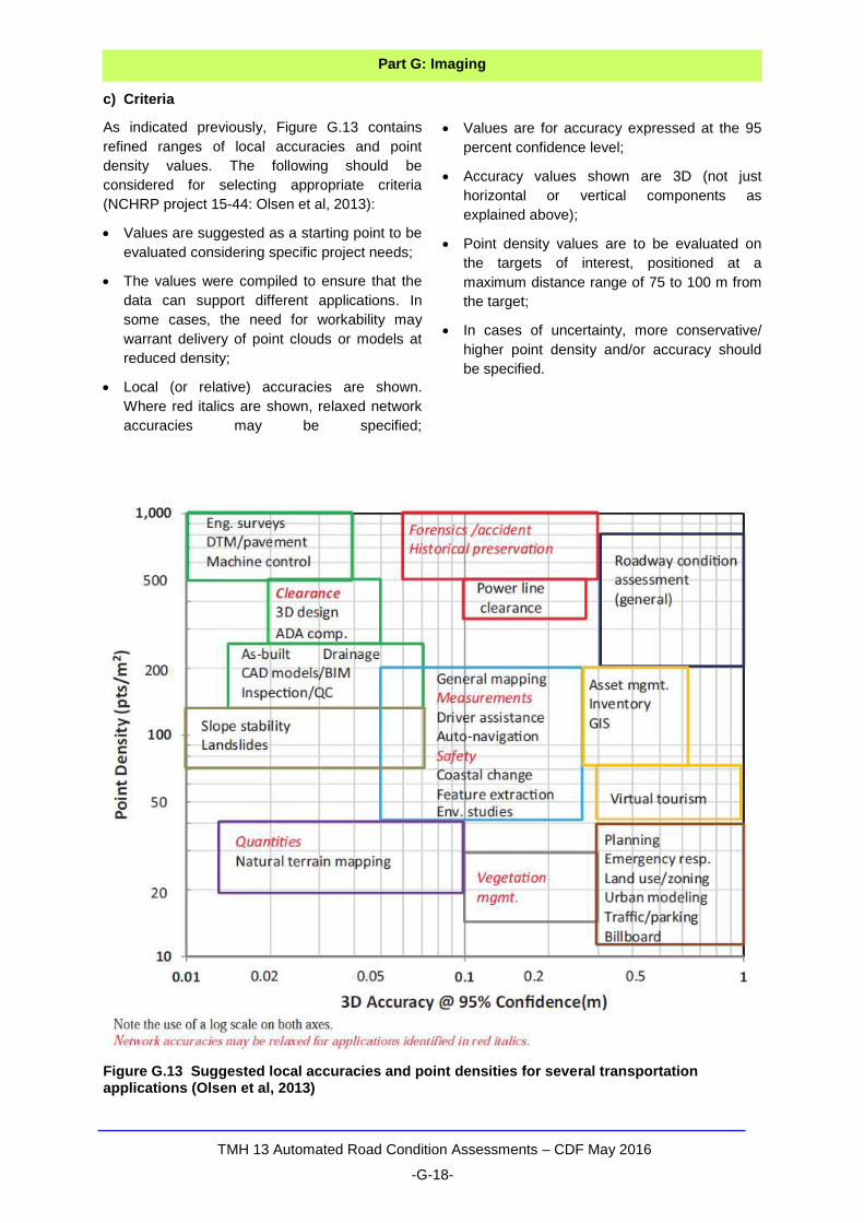
TMH 13 Automated Road Condition Assessments – CDF May 2016
-G-18-
Part G: Imaging
c) Criteria
As indicated previously, Figure G.13 contains
refined ranges of local accuracies and point
density values. The following should be
considered for selecting appropriate criteria
(NCHRP project 15-44: Olsen et al, 2013):
Values are suggested as a starting point to be
evaluated considering specific project needs;
The values were compiled to ensure that the
data can support different applications. In
some cases, the need for workability may
warrant delivery of point clouds or models at
reduced density;
Local (or relative) accuracies are shown.
Where red italics are shown, relaxed network
accuracies may be specified;
Values are for accuracy expressed at the 95
percent confidence level;
Accuracy values shown are 3D (not just
horizontal or vertical components as
explained above);
Point density values are to be evaluated on
the targets of interest, positioned at a
maximum distance range of 75 to 100 m from
the target;
In cases of uncertainty, more conservative/
higher point density and/or accuracy should
be specified.
Figure G.13 Suggested local accuracies and point densities for several transportation applications (Olsen et al, 2013)
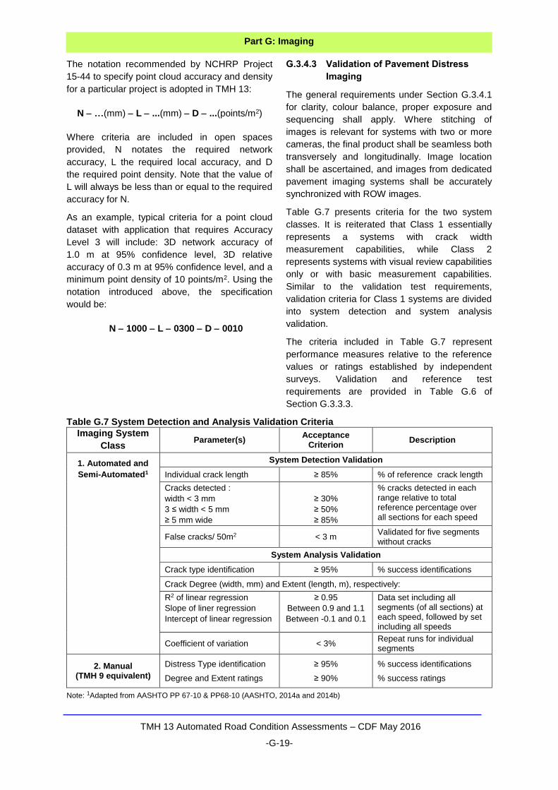
TMH 13 Automated Road Condition Assessments – CDF May 2016
-G-19-
Part G: Imaging
The notation recommended by NCHRP Project
15-44 to specify point cloud accuracy and density
for a particular project is adopted in TMH 13:
N …(mm) L ...(mm) D ...(points/m2)
Where criteria are included in open spaces
provided, N notates the required network
accuracy, L the required local accuracy, and D
the required point density. Note that the value of
L will always be less than or equal to the required
accuracy for N.
As an example, typical criteria for a point cloud
dataset with application that requires Accuracy
Level 3 will include: 3D network accuracy of
1.0 m at 95% confidence level, 3D relative
accuracy of 0.3 m at 95% confidence level, and a
minimum point density of 10 points/m2. Using the
notation introduced above, the specification
would be:
N 1000 L 0300 D 0010
G.3.4.3 Validation of Pavement Distress
Imaging
The general requirements under Section G.3.4.1
for clarity, colour balance, proper exposure and
sequencing shall apply. Where stitching of
images is relevant for systems with two or more
cameras, the final product shall be seamless both
transversely and longitudinally. Image location
shall be ascertained, and images from dedicated
pavement imaging systems shall be accurately
synchronized with ROW images.
Table G.7 presents criteria for the two system
classes. It is reiterated that Class 1 essentially
represents a systems with crack width
measurement capabilities, while Class 2
represents systems with visual review capabilities
only or with basic measurement capabilities.
Similar to the validation test requirements,
validation criteria for Class 1 systems are divided
into system detection and system analysis
validation.
The criteria included in Table G.7 represent
performance measures relative to the reference
values or ratings established by independent
surveys. Validation and reference test
requirements are provided in Table G.6 of
Section G.3.3.3.
Table G.7 System Detection and Analysis Validation Criteria
Imaging System
Class Parameter(s)
Acceptance Criterion
Description
1. Automated and
Semi-Automated1
System Detection Validation
Individual crack length ≥ 85% % of reference crack length
Cracks detected :
width < 3 mm
3 ≤ width < 5 mm
≥ 5 mm wide
≥ 30%
≥ 50%
≥ 85%
% cracks detected in each range relative to total reference percentage over all sections for each speed
False cracks/ 50m2 < 3 m Validated for five segments without cracks
System Analysis Validation
Crack type identification ≥ 95% % success identifications
Crack Degree (width, mm) and Extent (length, m), respectively:
R2 of linear regression
Slope of liner regression
Intercept of linear regression
≥ 0.95
Between 0.9 and 1.1
Between -0.1 and 0.1
Data set including all segments (of all sections) at each speed, followed by set including all speeds
Coefficient of variation < 3% Repeat runs for individual segments
2. Manual (TMH 9 equivalent)
Distress Type identification
Degree and Extent ratings
≥ 95%
≥ 90%
% success identifications
% success ratings
Note: 1Adapted from AASHTO PP 67-10 & PP68-10 (AASHTO, 2014a and 2014b)
TMH 13 Automated Road Condition Assessments – CDF May 2016
-G-20-
Part G: Imaging
G.3.5 Control Testing
Control testing should be performed from time to
time during the survey to ensure continued
validity of the systems and methods. Daily and
weekly quality control procedures complement
control testing through early detection and
correction of quality issues. Operational and
quality control procedures are provided in Section
G.4.
Control testing should be performed on validation
sections and the same criteria as used for
validation shall apply. However, control testing
need not be performed on all validation sections,
and normally control testing on two or three sites
would suffice.
Control testing for systems producing 3D point
clouds, shall be performed on validation datasets
that consist of more than 20 validation points.
Whilst it should be attempted to position
validation sites close to the centre of operations,
control testing using these sites may not always
be practical for large networks. In such cases,
dedicated control sections may be established at
strategic positions spread geographically
throughout the survey area. In addition, for
control testing where manual distress ratings are
involved, the use of different control sites and
rotation of these sites are recommended to
reduce the influence of human subjectivity.
Similar to validation sites, agencies (or third
parties) are responsible for the selection and
characterisation of dedicated control sites.
Control testing should be performed on a regular
basis as part of the survey process. If control
testing shows that the collected data are no
longer valid, the survey shall be ceased until the
cause of the problem can be identified. Any data
collected since the last successful control test
should be discarded and re-collected.
It should be obvious that the cost and time
implications of a failed control test are severe.
For this reason, control testing should be carried
out as frequently as possible within the
constraints of the network and survey budget.
The frequency of testing is basically a
compromise between the cost of control testing
(which not only delays the survey, but requires
additional time and travel), and the risk of re-
collecting all data collected since the last control
test. As a minimum for large projects, control
testing shall be conducted on a monthly basis.
For smaller projects control testing shall be
conducted in five stages (equally spaced in terms
of length surveyed) during the survey process.
TMH 13 Automated Road Condition Assessments – CDF May 2016
-G-21-
Part G: Imaging
G.4 Operational and Quality Control Procedures
G.4.1 Introduction
Part A addresses the need for a quality control
plan as an aid in achieving reliable, accurate, and
complete surveillance data. Previous sections
introduced calibration, validation and control
testing which are key imaging systems related
quality control activities. This section deals with
timely operational and data checks and methods
to mitigate the risk of producing data of
unacceptable quality.
It should be noted that while basic operational
aspects and their influence on imaging are
included, operators of imaging systems should –
in addition to the elements covered in this section
– have an in-depth understanding of the influence
of all operational elements on the imaging
process. Relevant standards and operational
manuals should be consulted for detailed
operational procedures.
The network manager is not responsible for
performing daily checks or following of proper
operational procedures. However, a proper
understanding of the elements that influence
measurement and of the procedures that a
contractor should perform each day, will allow the
network manager to exercise better control over
the measurement process. The guidelines in this
section thus focus on how operational
procedures can be controlled during the survey to
ensure data quality.
G.4.2 Operational Procedures for Imaging
Systems
Before a survey can start each day, specific
system checks should be performed in an official
and orderly way at the hand of an official “Check
List”. The operator will sign the check list at the
end of the procedure and thereby generate a
traceable quality assurance record as part of the
Quality Control Plan (See Part A).
The contractor’s check list will depend on the
survey vehicle and imaging system type, and the
recommendations from the manufacturers. As a
minimum, the check list shall include:
Vehicle: The general condition of the vehicle
and functioning of components shall be
checked. Safety related aspects, such as
indicators, hazards, dedicated safety lights,
arrows and other signs shall be visible, in
good condition and working order. Check the
condition and pressure of the vehicle tyres
and all spare tyres.
Batteries/ Power Supply/ Cabling: Where
applicable, ensure that batteries are fully
charged for both computers and the
measuring device. Check that power supplies
and all cabling are on board and that all
connections are good.
Imaging Hardware: All cameras, other
imaging components and enclosures, should
be securely mounted, correctly aligned, and
clean. Check that all imaging components and
the computer system with monitors are
functioning properly.
Imaging Software: Onboard systems for data
acquisition and real-time monitoring (of
imaging and other data types) should be
ascertained for proper functioning and
integration. Where used, reference data
bases and shape files for storing geometric
location and associated attribute information
should also be loaded and checked.
Warm-up Time: The measuring and data
acquisition systems should be subjected to
sufficient warm-up time according to the
manufacturer’s recommendations.
Imagery and associated data shall be monitored
periodically throughout the day for completeness
and to detect any changes in quality. At the end
of each day of survey, back-up of data and a
review of imagery and other data are required.
This allows the operators to identify issues, take
corrective action, and re-collect the problem
segments before leaving an area. The operators
shall keep daily logs of activities, including all
quality control activities. The Network Manager
shall be notified of any unusual circumstances.
Whilst the network manager cannot ensure that
all checks are rigorously performed each day,
spot checks shall be performed from time to time.
These checks should be performed randomly on
a weekly or two-weekly basis. During each
check, the operator should be asked to stop the
vehicle and a control check should be performed.
Control checks may include inspection of system
calibration and validation certificates, the
condition and functioning of the survey vehicle
and imaging system, as well as inspection of
collected imagery and other data.
TMH 13 Automated Road Condition Assessments – CDF May 2016
-G-22-
Part G: Imaging
G.4.3 Data Capturing, Processing,
Management and Documentation
G.4.3.1 Data Capturing and Processing
The contract specifications should provide details
on the format required for the captured data. As a
minimum, the specifications should state the
format of the required files (e.g. ASCII, JPEG,
MOV, LAS, spreadsheet format) and the required
data fields for processed data deliverables.
In addition to the requirements of TMH 13 (See
Section G.3), TMH 18 and TMH 22 should be
consulted for items to be collected and reported.
The agency may provide database shells or
shape files to streamline data capturing and
facilitate identification of network segments,
thereby reducing any associated errors. The
contractor should also provide a definition sheet
to define any codes or abbreviations used in the
file and column naming. Details of the format in
which the output will be provided should ideally
be submitted with the contractor’s quality control
plan.
Digital video and/or photo mosaic should be
provided in a common format. For photos, these
would typically be supplied as TIFF, JPEG or
PNG and for video as AVI or MOV with a
common, near-lossless compression code (if
applicable). Apart from essential inventory and/or
condition data, the following should be reported
as a minimum (AASHTO, 2014a):
Asset identifier (ID), road number, link and
segment identification, and other details (e.g.
lane, direction)
Unique image identifier together with image
location (latitude and longitude) using the first
shoulder side data point;
Image scale, which should be equal in both
directions;
For 3D imaging used for asset management or
inventory mapping, a geo-referenced point cloud
should always be delivered. Classification of data
points is encouraged and can simplify the use of
data. However, classification types and
categories should be established and clearly
specified by the agency. It is recommended that
the LAS format or other approved format be used
for point cloud delivery. The use of multiple
formats and data transfers shall be minimized
during workflows (Olsen et al, 2013).
Digital video or photo imagery shall be co-
acquired with 3D imaging by laser scanners or
any non-photogrammetric systems. Imagery
should preferably be geo-referenced to point
clouds as a visual reference, especially for
feature extraction and validation.
Point clouds shall be obtained using the optimum
navigation trajectory of the vehicle that has had
each imaging pass shifted via rigid body
translation to fit local transformation (or control)
points for the project. Survey control point
locations and accuracy shall be reported (X,Y Z,
ID, standard deviations, residuals, etc.).
Trajectories for each pass of the imaging survey
vehicle should be provided in common format,
typically KMZ or SHP. A field with modelled error
estimates throughout the trajectory should be
included with the trajectory data (Olsen et al,
2013).
Outputs from modelling of registered point clouds
will depend on the project requirements and
should be specified to conform to the agency’s
graphic standards. Features are typically
extracted and modelled as 3D CAD, GIS, or BIM
objects. Modelling requirements should be clearly
specified including file size limitations, desired
data density, and completion of optimization
procedures. Details of the modelling procedures
and quality control of the results should ideally be
submitted with the contractor’s quality control
plan.
Any useful comments that may affect image
analysis should be reported. As an example for
pavement distress imaging analysis, aspects
such as crack seals, railroad tracks, and
excessive pavement marking should be reported.
The operator should flag any data files or parts
thereof for which measurements are regarded as
unusual or files recorded under non-optimal
conditions. Operators should therefore be trained
not only in the system operation aspects, but also
in the interpretation of data and the potential
impact of pavement, environmental and other
parameters on data accuracy and precision.
G.4.3.2 Data Management
A copy of the dataset (video, point cloud etc.) at
the highest level of processing should always be
requested from service providers for future
reference or data mining. Attention should be
given to handling of large and complex datasets
generated by imaging systems. Aspects of data
TMH 13 Automated Road Condition Assessments – CDF May 2016
-G-23-
Part G: Imaging
management included in this section were largely
obtained from NCHRP 15-44 (Olsen et al, 2013).
It should be recognised that the bulk of the data
falls into two categories, namely read-only and
mutable data. Read-only refers to data that do
not or should not change, typically large files
containing raw measurements or imagery.
Mutable refers to changeable or derived data,
typically much smaller files containing extracted
and processed information.
After initial processing, e.g. geo-referencing and
classification, the core imagery should not
change and can be considered read-only. Once
stored in the appropriate format and location and
backed up, these data do not need to be part of
the incremental backups or version management.
By separating these large sets of static data from
other data, management is simplified. Special
consideration should be given to protection of
read-only files because much of this data may
operate outside usual IT channels. In particular,
read-only files must be guaranteed to remain
immutable and should be protected from
accidental editing, deletion, renaming, or
relocation.
Extracted data are derived from imagery or
measurement, e.g. locations and dimensions of
features such as road markings or signage.
Different levels of processing can be facilitated
using a variety of potentially manual, semi-
automated, and fully automated software tools.
With each processing step, the value of the
information increases, whilst the incremental
storage required normally reduces. Regardless of
the extraction and/or higher level processing
method used, potential errors may be introduced
in each step. Specifications should therefore
cater for proper reporting of data lineage. As a
minimum for 3D imaging, a metadata file
containing project related data (as defined by the
agency) should accompany each project file.
Information resulting from these processes is
usually mutable, consisting of smaller and more
manageable files which should be included in
normal agency management, IT procedures and
policies.
The medium of data delivery should be specified
and is typically via external hard drives which can
be used as host drives, eliminating the time
required to copy files. Whichever type of drive is
used, identical duplicate data should be sub-
mitted on a second drive. The backup or second
drive should be verified as soon as possible after
delivery, before placed in secure storage.
The specifications should stipulate the deadline
for delivery of data files on completion of the
survey. It is important to minimize delays
between the time of survey and data analysis, in
order for errors to be identified as soon as
possible. Ideally, some data files should be given
to the network manager while the survey is in
progress, so that the data can be checked and
any inconsistencies identified at an early stage.
G.4.3.3 Documentation and Deliverables
Apart from documentation outlined under Part A,
imaging surveys, and especially high-end 3D
imaging surveys, require clear documentation of
the quality and lineage of the data to maximize
the return on investment, future use and usability
for multiple applications within the agency. As
such, this subsection largely focuses on
documentation and deliverables typically required
after completion of 3D imaging surveys.
In general, all systems included under TMH 13
include cameras. A camera calibration report
(interior orientation) and image geo-referencing
information (exterior orientation) are required for
all cameras and images, respectively.
The outline to follow is an extract from NCHRP
15-44 (Olsen et al, 2013). A survey narrative
report should be completed, including the
following minimum information:
Project name and location identifier
Survey date, time, weather conditions, limits
and purpose
Project datum, epoch and units
System calibration report
Survey control points found, held and set (see
Control Survey Report)
Personnel, equipment, and surveying
methodology employed
Problems encountered, if any
Other supporting survey information such as
GPS observation logs
Dated signature and seal (if licensure is
required) of the surveyor/ engineer in charge
Higher order survey control networks may be
required depending on the application.
Traceability back to the published primary control
and reproducibility by an independent 3rd party
must be ascertained.
TMH 13 Automated Road Condition Assessments – CDF May 2016
-G-24-
Part G: Imaging
To this end, the data lineage shall be clearly
defined and documented in a control survey
report containing the following minimum
information:
Primary control held or established
Project control held or established
Local transformation/ control points
Validation points
Adjustment report for control and validation
points
Base station observation logs (occupation
data, obstruction diagram, atmospheric
condition, etc.)
GPS accuracy report with details on time,
duration, and location of loss of signal lock
GPS satellite visibility and PDOP reports
IMU accuracy report
Trajectory reports including locations of loss
of signal lock exceeding a specified threshold
(typically 60 seconds) and operating speeds
during acquisition
In addition to the control survey report where the
application requires this level of accuracy, the
following data processing documentation should
be provided:
Trajectory analysis and quality control
Adjustment report
Registration statistics
System calibration/ model fitting statistics
Detailed metadata files
Datasets to be delivered include:
Point cloud
o Raw data
o Geo-referenced data
o Classified data
Associated imagery:
o Video
o Photo mosaic
Modelled data may include:
o DTM
o CADD, BIM
o GIS database files
o Other formats
Survey control points
Trajectory
G.4.4 Data Checking and Troubleshooting
Periodic testing of control sites is one of the key
quality control measures and results are used for
both quality control and acceptance (see Section
G.3.5). It is reiterated that control testing needs to
be performed regularly so that the quantity of
collected data is manageable when resurveying
is required.
In addition, the network manager should perform
a series of acceptance checks on the final
condition database or batches of data and
imagery received.
a) General
Global database checks may be performed as
manual screening, execution of saved queries, or
an automated or semi-automated series of error
checks. In general, database checks include
(Pierce et al, 2013):
Compliance with required format even if a
database shell was provided. Automated
checks or queries may not function correctly if
formats are incorrect.
Location accuracy and checks for missing
segments using segment files or GIS.
Data completeness checks. For example by
scrutinizing zero or default values, or the
number of events recorded by segment.
Data consistency checks using engineering
judgement or doing logic tests to identify data
that do not make sense.
Screening for out of range data using
predefined triggers, minimum and maximum
values. For example, the area of patching
cannot be greater than the segment area.
More detailed checks should be performed on a
sample of data. The sample size typically varies
between 5 and 10 percent, depending on the
network size. Whilst any sampling method may
be used (viz. random, systematic, stratified,
clustered or a combination), it should be noted
that reference values for these sites normally do
not exist. Sections with which the manager is
familiar with may therefore be selected. The
objective of these checks should be to ensure the
measurements correspond with basic
engineering judgement, and that the data are
consistent with that of earlier surveys.
Alternatively, blind sites may be selected which
are unknown to the contractor but with conditions
known to the agency. Independent resurveys of
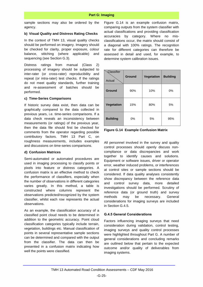
TMH 13 Automated Road Condition Assessments – CDF May 2016
-G-25-
Part G: Imaging
sample sections may also be ordered by the
agency.
b) Visual Quality and Distress Rating Checks
In the context of TMH 13, visual quality checks
should be performed on imagery. Imagery should
be checked for clarity, proper exposure, colour
balance, stitching (where applicable) and
sequencing (see Section G.3).
Distress ratings from manual (Class 2)
processing of imagery should be subjected to
inter-rater (or cross-rater) reproducibility and
repeat (or intra-rater) test checks. If the ratings
do not meet quality standards, further training
and re-assessment of batches should be
performed.
c) Time-Series Comparisons
If historic survey data exist, then data can be
graphically compared to the data collected in
previous years, i.e. time-series comparisons. If a
data check reveals an inconsistency between
measurements (or ratings) of the previous year,
then the data file should first be checked for
comments from the operator regarding possible
contributory factors. TMH 13 Part C, on
roughness measurements, includes examples
and discussions on time-series comparisons.
d) Confusion Matrices
Semi-automated or automated procedures are
used in imaging processing to classify points or
pixels into feature or distress categories. A
confusion matrix is an effective method to check
the performance of classifiers, especially when
the number of observations in different categories
varies greatly. In this method, a table is
constructed where columns represent the
observations predicted/recognized by the system
classifier, whilst each row represents the actual
observations.
As an example, the classification accuracy of a
classified point cloud needs to be determined in
addition to the geometric accuracy. Point cloud
classification categories typically include terrain,
vegetation, buildings etc. Manual classification of
points in several representative sample sections
can be determined and compared with the output
from the classifier. The data can then be
presented in a confusion matrix indicating how
well the points were classified.
Figure G.14 is an example confusion matrix,
comparing outputs from the system classifier with
actual classifications and providing classification
accuracies by category. Where no mis-
classifications occur, the matrix should consist of
a diagonal with 100% ratings. The recognition
rate for different categories can therefore be
assessed in detail and used, for example, to
determine system calibration issues.
Classifier
Actual
Ground Vegetation Building
Ground 90% 10% 0%
Vegetation 15% 80% 5%
Building 0% 5% 95%
Figure G.14 Example Confusion Matrix
All personnel involved in the survey and quality
control processes should openly discuss non-
compliance or data discrepancies and work
together to identify causes and solutions.
Equipment or software issues, driver or operator
error, weather induced problems, or interferences
at control sites or sample sections should be
considered. If data quality analyses consistently
show discrepancy between the reference data
and control survey data, more detailed
investigations should be performed. Scrutiny of
reference data (or ground truth) and survey
methods may be necessary. General
considerations for imaging surveys are included
in Section G.4.5.
G.4.5 General Considerations
Factors influencing imaging surveys that need
consideration during validation, control testing,
imaging surveys and quality control processes
were highlighted throughout Part G. A number of
general considerations and concluding remarks
are outlined below that pertain to the expected
outcome and/or quality of deliverables from
imaging systems.
TMH 13 Automated Road Condition Assessments – CDF May 2016
-G-26-
Part G: Imaging
While ROW imaging will capture objects
within range and line of sight, objects such as
drainage ditches and culvert details may be
difficult to see or non-visible in the dataset or
image.
Scanning geometry (position and orientation
of scanner or camera with respect to object of
interest) determines how well objects are
captured. For example, dedicated pavement
imaging systems capture detailed pavement
surface data, but are not configured to acquire
data on surrounding features.
System performance at various sun angles
and intensities. Imaging with cameras should
be limited to a specific time period of the day
(i.e. 9 am to 4 pm) to avoid driving into, or
away from the sun which would be at a low
altitude. Direct sunlight into the camera will
blind the camera and render the images void.
Performance under various lighting
conditions. In general imaging in bad light
should be avoided. The camera will try to
compensate for the bad light by decreasing
the shutter speed. This will lead to “smeared”
images of bad quality.
Performance at various humidity, temperature
and wind conditions. Wet pavements or
conditions that induce refraction should be
avoided, such as precipitation, steam, or heat
rising from surfaces.
Many pavement distress detection and
processing algorithms are in research and
development and focus primarily on cracks.
Systems may vary in terms of their ability to
detect crack width and length in all directions;
sensitivity of characteristics that define a
fissure (crack delineation); minimum
resolution versus delineation level and crack
angle, and resolution versus position of cracks
due to optical distortion (AASHTO, 2014b).
Data gaps may be caused by visibility
constraints during ROW imaging (such as
shadows or occlusions). It is therefore
recommended that surveys preferably be
done during low traffic periods. Alternatively,
implementation of a traffic rolling slowdown
behind the survey vehicle could be considered
to minimize vehicles creating data gaps. Data
gaps can also be filled in by doing multiple
passes.
Multiple passes with scanning lasers are often
performed. Overlapping scans provide higher
point density, remove data gaps, and offer
increased reliability from redundancy. In the
case of scans in opposite directions, a
minimum side overlap of 20 percent may be
specified. Comparison of elevation data from
side overlaps may be requested as supporting
documentation.
Scanning lasers do not penetrate water.
Highly reflective surfaces at close range can
be problematic, creating saturation and
blooming effects. Dark surfaces do not reflect
light well and can be problematic at long
ranges for some scanners.
Not all points in point clouds have the same
accuracy which introduces noise. The use of
single or isolated points should therefore be
avoided when making measurements.
However, whilst individual points may have
lower accuracies compared to conventional
surveying, objects can be modelled more
accurately due to the relatively high point
density, i.e. capturing of more detail.
Many algorithms used to process point cloud
data are in research and development. The
identification of features in point cloud data is
usually done by virtual surveying using semi-
automated or manual processes which can be
time consuming. A few automated processes
exist, but are limited to objects with simple,
standard geometric shapes (e.g. planes,
spheres and cylinders). Co-acquired camera
imagery with RGB colour mapped to the point
cloud can be valuable during the mapping/
measurement process. Point classification
(attributes such as what the point represents)
can also be done through manual, semi-
automated, and/or automated processing.
(Olsen et al, 2013)

TMH 13 Automated Road Condition Assessments – CDF May 2016
-G-27-
G.5 References
AASHTO. 2014a. AASHTO Provisional Standards PP68-10: Collecting Images of Pavement Surfaces for Distress Detection. American Association of State Highway Officials, Washington, D.C.
AASHTO. 2014b. AASHTO Provisional Standards PP67-10: Quantifying Cracks in Asphalt Pavement Surfaces from Collected Images Utilizing Automated Methods. American Association of State Highway Officials, Washington, D.C.
Austroads. 2006. Guide to Asset Management, Part 5E: Cracking. Publication No. AGAM05E/06. Austroads Ltd., Sydney, Australia.
Brown, D. and Thomsen, T. 2007. Generic Equipment Specification of Multi-Functional Road Data Collection Systems. East Asia Pacific Transport Unit, The World Bank, Washington, D.C.
Dynatest. 2010. Dynatest Road Surface Profiler Mark III. Dynatest (Pty) Ltd. <www.dynatest.com/functional-rsp.php>
Faber, F. 2014. Best Practice for Mobile LIDAR Survey Requirements: Discussion Paper. Austroads Technical Report AP-T269-14. Austroads Ltd., Sydney, Australia.
Faber, F., Bennet, P., Muller, W. and Ngo, H. 2014. Application of New Technologies to Improve Risk Management. Austroads Technical Report AP-T268-14. Austroads Ltd, Sydney, Australia.
Fugro. 2014. Fugro Roadware. <http://www.roadware.com/products/>
Inivit. 2010. Presentation - High Speed Digital Audit (HSDA). Inivit (Pty) Ltd, Pretoria, South Africa.
Kemendy, J. and Turner, K. 2008. Ground-Based LIDAR: Rock Slope Mapping and Assessment. Report FHWA-CFL/TD-08-006. Federal Highway Administration, Central Federal Lands Highway Division, CO, USA.
Nulty, M. and Noble, T. 2013. A Comparative Study Using LIDAR Digital Scanning and Photogrammetry. 3D Digital Documentation Summit, July 10-12, 2012, Presido, San Francisco, CA, USA.
Olsen, M.J., Roe, G.V. , Glennie, C., Persi, F., Reedy, M., Hurwitz, D., Williams, K., Tuss, H., Squellati, A. and Knodler, M. 2013. Guidelines for the Use of Mobile LIDAR in Transportation Applications. National Cooperative Highway Research Program (NCHRP) Report 748, Transportation Research Board, Washington, D.C.
Pavemetrics. 2010. Laser Road Imaging System (LRIS). PavementricsTM Systems Inc. <http://www.pavemetrics.com/index.html>
Pavemetrics. 2014. Laser Crack Measurement System (LCMS). PavementricsTM Systems Inc. <http://www.pavemetrics.com/index.html>
PIARC. 2012. Evaluating the Performance of Automated Pavement Cracking Measurement Equipment. Technical Committee CT 4.2 on Interactions Vehicle/Road. The World Road Association (PIARC), Paris, France.
Pierce, L.M., Mc Govern, G. and Zimmerman, K. 2013. Practical Guide for Quality Management of Pavement Condition Data Collection. U.S. Department of Transportation, Federal Highway Administration, Washington, D.C.
SANRAL. 2014. Presentation - RHINO Survey Vehicle. The South African National Roads Agency (SOC) Ltd. Pretoria, South Africa.
Trimble. 2014. Trimble MX8. <http://www.trimble.com/Imaging/Trimble-MX8.aspx>
Wang, K.C.P and Smadi, O. 2011. Transportation Research Circular Number E-C156: Automated Imaging Technologies for Pavement Distress Surveys, July 2011. Transportation Research Board, Washington, D.C.
Wang, K.C.P. 2013. 3D Laser Imaging for Pavement Survey at 60 mph and True 1mm Resolution - Oklahoma State University & WayLink. Presented at the Arizona Pavements & Materials Conference, Arizona State University MU, November 13 - 14, 2013.
Wix, R. 2012. RoadcrackTM - Measuring more than cracks. 7th Symposium on pavement surface characteristics. Norfolk, Virginia, September 19 - 22, 2012.
Wix,R. and Leschinski, R. 2012. Cracking - A Tale of Four Systems. ARRB Group Ltd. 25th ARRB Conference, Perth, Australia, 2012.
TMH 13 Automated Road Condition Assessments – CDF May 2016
-G-28-
G.6 Glossary
2D: Two-dimensional. Typically referring to data that has been mapped to a plane such as a map or plan (NCHRP 15-44, Olsen et al, 2013, p. 218).
3D: Three-dimensional. In a 3D Cartesian coordinate system (XYZ), there can be multiple Z values at any given XY coordinate (NCHRP 15-44, Olsen et al, 2013, p. 218).
3D imaging system: A non-contact measurement device used to produce a 3D representation (for example a point cloud) of an object or a site (ASTM E2544-10).
3D reconstruction: A process of creating a 3D model from data that is not 3D. For example, a series of 2D photographs of an object can be combined to produce a 3D model (NCHRP 15-44, Olsen et al, 2013, p. 218).
Absolute Accuracy: The level of accuracy that can be obtained in a global coordinate system (NCHRP 15-44, Olsen et al, 2013, p. 218).
Accuracy: Closeness of the agreement between the result of a measurement and a true value of the measurement (ASTM E2544-10). The degree to which a measurement, or the mean of a distribution of measurements, tends to coincide with the population mean (FHWA, Pierce et al, 2013, p.85).
Big Data: A popular term used to describe any collection of large structured or unstructured data sets that is difficult to process using traditional database or software techniques.
Blind site: Control site with location unknown to the survey team.
Calibration: “Set of operations that establish, under specified conditions, the relationship between values of quantities indicated by a measuring instrument or measuring system, or values represented by a material measure or a reference material, and the corresponding values realized by standards” (ASTM E2544-10). A system calibration corrects for inherent system characteristic or manufacturing errors and produces a set of parameters that remains constant as long as the hardware is not adjusted or disturbed. In 3D imaging, this should not be confused with geometric correction (sometimes called a site calibration or local transformation (NCHRP 15-44, Olsen et al, 2013, p. 220).
Control network: In 3D imaging: A collection of control points with stated coordinate uncertainties, in a single coordinate system (ASTM E2544-10).
Control point: In 3D imaging: An identifiable point (visible or inferable) which is a member of a control network (ASTM E2544-10).
Control sites: Roadway segments (that may coincide with validation sites) with known condition or other characteristic values of interest, measured by the agency or third party for use as reference values for comparison with data collected from time to time on the designated sections (control testing) during the survey to verify continued use of valid methods and equipment as part of the quality control process (FHWA, Pierce et al, 2013, p. 85).
Confusion matrix: A table to show the effectiveness of an algorithm comparing the algorithms predicted results to actual results and typically used for a classification accuracy assessment (NCHRP 15-44, Olsen et al, 2013, p. 221).
Crack: A discontinuity or break in the integrity of the pavement surface, usually a narrow opening or partial fracture in a pavement surface. Cracks may be transverse, longitudinal, irregular, single, grouped, or interconnected crocodile pattern or blocks with varying space between them. Except on continuously reinforced concrete pavements, cracks almost invariably represent a pavement defect (Austroads, Guide to Asset Management Part 5E: Cracking, 2006).
Detectability: The threshold or limiting crack width for detection by a crack/ distress detection system (Austroads, Guide to Asset Management Part 5E: Cracking, 2006).
Data processing: All activities that are conducted to convert the raw data/ imagery collected in the field surveys to useful information. These activities can be manually done by a reviewer/assessor, semi-automated by a reviewer/assessor facilitated by software, or automated by software using algorithms with minimal human involvement.
DGPS/GNSS: Differential GPS/GNSS. A system that uses a network of fixed ground based reference stations to broadcast the difference between the positions indicated by the GPS/GNSS satellite systems and the known fixed positions (definition after Wikepedia, 2007).

TMH 13 Automated Road Condition Assessments – CDF May 2016
-G-29-
Distress rating: A process where the severity (degree) and extent of different types of distresses are visually assessed by a certified assessor. Traditionally this is conducted by a ‘walk over’ or ‘windshield’ assessment. In the context of TMH 13, assessments are performed by a virtual tour using imagery of the road asset.
Distress measurement: Assigning dimensional quantities such as length and width to a distress through manual, semi-automated or automated processing of collected imagery. Manual measurements can also be conducted directly in the field to serve as reference values for validation of system detection capabilities.
Frame imaging: Or are scanning uses a two-dimensional array of pixels in a conventional sequence of snapshots (Wang and Smadi, 2011, p. 4).
Geo-reference: The process of assigning a coordinate system and location information to a point or points in space (NCHRP 15-44, Olsen et al, 2013, p. 224).
Geometric correction: A geometric correction or adjustment is done to correct for errors in the GNSS and IMU positioning information by adjusting the scan data to control or between adjacent passes. This correction would be applied uniquely for each project (NCHRP 15-44, Olsen et al, 2013, p. 223).
IMU: Inertial Measurement Unit. A device which utilises a combination of gyroscopes and accelerometers to provide velocity and orientation information (NCHRP 15-44, Olsen et al, 2013, p. 225).
Line scan imaging: Uses a single line of sensor pixels to build up a two dimensional digital image. The second dimension results from the motion of the sensors/ imaging system or the object (Wang and Smadi, 2011, p. 4).
LIDAR: Light Detection and Ranging. A method of measuring the flight time of a beam of light to calculate range to objects at predetermined angular increments, implemented using a laser scanner and resulting in a point cloud (NCHRP 15-44, Olsen et al, 2013, p. 226).
Mobile LIDAR System (MLS): A mobile ground-based system (as appose to airborne LIDAR systems) utilising the at least one laser scanner.
Pavement image: A presentation of the pavement that describes a characteristic (gray scale, colour, temperature, elevation, etc.) of a matrix of point (pixels) on the pavement (AASHTO PP 68-10).
Photogrammetry: The science of making measurements from photographs, especially for recovering exact positions of surface points (<en.wikipedia.org/wiki/photogrammetry>, 2014).
Precision: See “Repeatability”
Point cloud: A collection of data points in 3D space (frequently in the hundreds of thousands), for example as obtained using a 3D imaging system (ASTM E2544-10).
Range imaging: Produces the 3D structure of a scene by using line projectors and high-speed cameras to construct a depth map of surface points through triangulation techniques. Each pixel of a range image expresses the distance between a known reference frame and a visible point in the scene.
Reference value: A value that serves as an agreed-upon reference for comparison, and which is derived as a theoretical or established value, based on scientific principles, and assigned or certified value, based on experimental work of some national or international organization, or a consensus or certified value, based on collaborative experimental work under the auspices of a scientific or engineering group. Reference value is also known as “ground truth” (FHWA, Pierce et al, 2013, p.88).
Resolution: The resolution of a device specifies the smallest measurement increment that the device is capable of, or the degree of detail that can be seen.
Repeatability: Degree of variation among the results obtained by a single operator using the same test method. The term is also used to designate test precision under a single operator.
Reproducibility: Degree of variation among the results obtained by different operators using the same test method.
Relative Accuracy: The level of accuracy that can be obtained within a local coordinate system (NCHRP 15-44, Olsen et al, 2013, p. 230)

TMH 13 Automated Road Condition Assessments – CDF May 2016
-G-30-
Registration: The process of determining and applying to two or more datasets the transformations that locate each dataset in a common coordinate system so that the datasets are aligned relative to each other (ASTM E2544-10).
RMSE: Root Mean Squared Error. Measures how much error exists between two datasets, usually between predicted values and observed values. For example, results from a LIDAR survey: RMSE takes the difference between each LIDAR value and surveyed value (control point), square the difference, and divide the sum of all values by the number of observations (<http://gisgeography.com/root-mean-square-error-rmse-gis/>, 2014).
RTK GPS: Real time kinematic GPS. An enhancement to satellite navigation that utilised carrier phase measurements for better positioning; allows for GPS corrections in real time (NCHRP 15-44, Olsen et al, 2013, p. 230).
Scaled frame image: An image with assigned horizontal and vertical scales based on known/ reference measurements of objects. More advanced systems use the principles of photogrammetry to geo-reference each pixel in the image.
Time-history: A set of successive periodic measurements of pavement condition over time on the same roadway section, used to evaluate pavement performance and as a data quality check.
Validation: The process of determining if a measurement device or system, when operated according to an established procedure and within established operating ranges, can operate effectively, reproducibly, delivers data that meet certain criteria.
Validation site: A roadway segment with known condition (or other characteristics) determined by the agency or a third party used to validate measurement devices or systems for acceptance before production measurements starts.

TMH 13 Automated Road Condition Assessments – CDF May 2016
-G-31-
APPENDIX G-1
MOBILE LIDAR SUGGESTED
APPLICATION MATRIX
(NCHRP PROJECT 15-44, OLSEN et al, 2013)
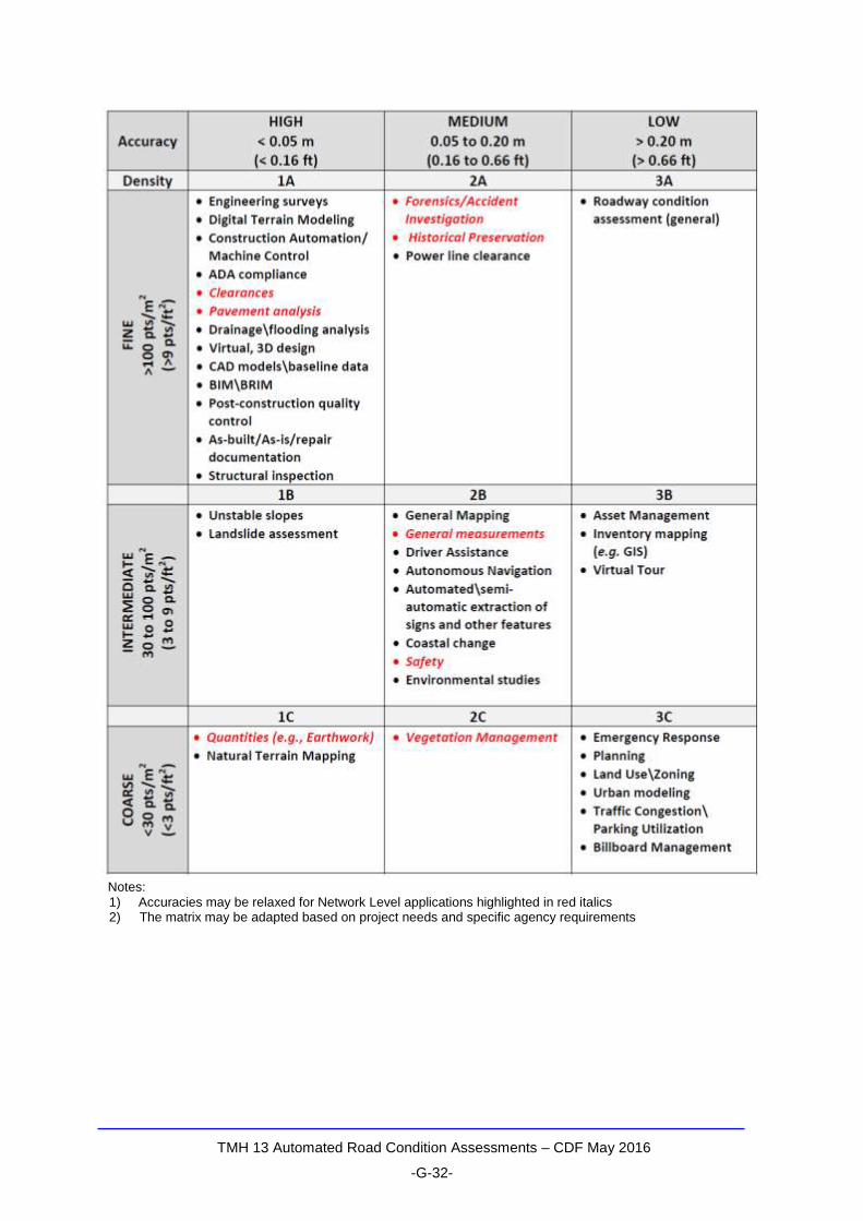
TMH 13 Automated Road Condition Assessments – CDF May 2016
-G-32-
Notes: 1) Accuracies may be relaxed for Network Level applications highlighted in red italics 2) The matrix may be adapted based on project needs and specific agency requirements
TMH 13 Automated Road Condition Assessments – CDF May 2016
-G-33-
APPENDIX G-2
CRACK DEFINITIONS FOR AUTOMATED
ANALYSIS METHODS
(FLEXIBLE PAVEMENTS)
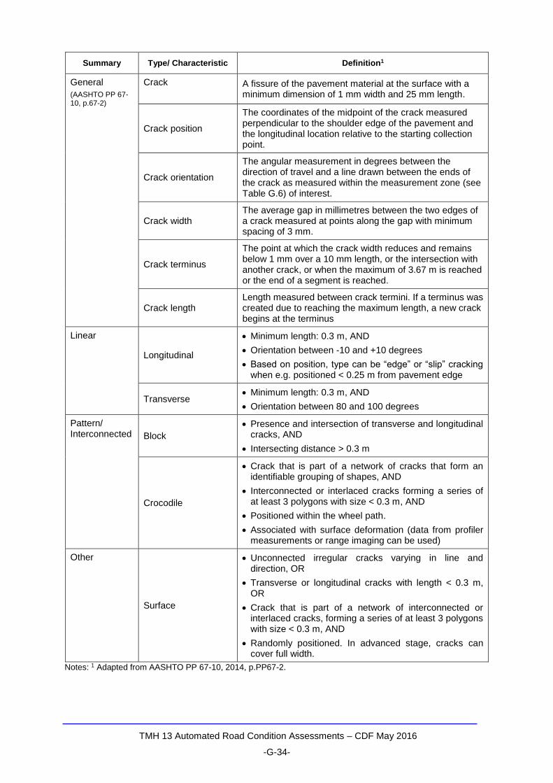
TMH 13 Automated Road Condition Assessments – CDF May 2016
-G-34-
Summary Type/ Characteristic Definition1
General
(AASHTO PP 67-10, p.67-2)
Crack
A fissure of the pavement material at the surface with a minimum dimension of 1 mm width and 25 mm length.
Crack position
The coordinates of the midpoint of the crack measured perpendicular to the shoulder edge of the pavement and the longitudinal location relative to the starting collection point.
Crack orientation
The angular measurement in degrees between the direction of travel and a line drawn between the ends of the crack as measured within the measurement zone (see Table G.6) of interest.
Crack width The average gap in millimetres between the two edges of a crack measured at points along the gap with minimum spacing of 3 mm.
Crack terminus
The point at which the crack width reduces and remains below 1 mm over a 10 mm length, or the intersection with another crack, or when the maximum of 3.67 m is reached or the end of a segment is reached.
Crack length Length measured between crack termini. If a terminus was created due to reaching the maximum length, a new crack begins at the terminus
Linear
Longitudinal
Minimum length: 0.3 m, AND
Orientation between -10 and +10 degrees
Based on position, type can be “edge” or “slip” cracking when e.g. positioned < 0.25 m from pavement edge
Transverse Minimum length: 0.3 m, AND
Orientation between 80 and 100 degrees
Pattern/ Interconnected
Block
Presence and intersection of transverse and longitudinal cracks, AND
Intersecting distance > 0.3 m
Crocodile
Crack that is part of a network of cracks that form an identifiable grouping of shapes, AND
Interconnected or interlaced cracks forming a series of at least 3 polygons with size < 0.3 m, AND
Positioned within the wheel path.
Associated with surface deformation (data from profiler measurements or range imaging can be used)
Other
Surface
Unconnected irregular cracks varying in line and direction, OR
Transverse or longitudinal cracks with length < 0.3 m, OR
Crack that is part of a network of interconnected or interlaced cracks, forming a series of at least 3 polygons with size < 0.3 m, AND
Randomly positioned. In advanced stage, cracks can cover full width.
Notes: 1 Adapted from AASHTO PP 67-10, 2014, p.PP67-2.