Embed Size (px)
Citation preview
Principles of Parallel Algorithm Design
Ananth Grama, Anshul Gupta, George Karypis, and Vipin Kumar
To accompany the text “Introduction to Parallel Computing”,Addison Wesley, 2003.

Chapter Overview: Algorithms and Concurrency
• Introduction to Parallel Algorithms
– Tasks and Decomposition– Processes and Mapping– Processes Versus Processors
• Decomposition Techniques
– Recursive Decomposition– Recursive Decomposition– Exploratory Decomposition– Hybrid Decomposition
• Characteristics of Tasks and Interactions
– Task Generation, Granularity, and Context– Characteristics of Task Interactions.
– Typeset by FoilTEX – 1
Chapter Overview: Concurrency and Mapping
• Mapping Techniques for Load Balancing
– Static and Dynamic Mapping
• Methods for Minimizing Interaction Overheads
– Maximizing Data Locality– Minimizing Contention and Hot-Spots– Overlapping Communication and Computations– Replication vs. Communication– Group Communications vs. Point-to-Point Communication
• Parallel Algorithm Design Models
– Data-Parallel, Work-Pool, Task Graph, Master-Slave, Pipeline, and HybridModels
– Typeset by FoilTEX – 2
Preliminaries: Decomposition, Tasks, andDependency Graphs
• The first step in developing a parallel algorithm is to decomposethe problem into tasks that can be executed concurrently
• A given problem may be docomposed into tasks in manydifferent ways.
• Tasks may be of same, different, or even interminate sizes.
• A decomposition can be illustrated in the form of a directedgraph with nodes corresponding to tasks and edges indicatingthat the result of one task is required for processing the next.Such a graph is called a task dependency graph.
– Typeset by FoilTEX – 3
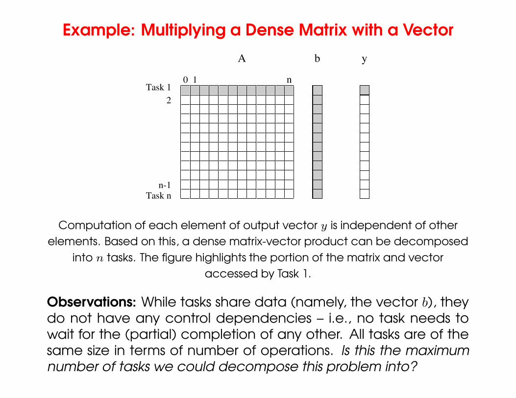
Example: Multiplying a Dense Matrix with a Vector
b yA
10 nTask 1
Task nn-1
2
Computation of each element of output vector y is independent of otherelements. Based on this, a dense matrix-vector product can be decomposed
into n tasks. The figure highlights the portion of the matrix and vectoraccessed by Task 1.
Observations: While tasks share data (namely, the vector b), theydo not have any control dependencies – i.e., no task needs towait for the (partial) completion of any other. All tasks are of thesame size in terms of number of operations. Is this the maximumnumber of tasks we could decompose this problem into?
– Typeset by FoilTEX – 4
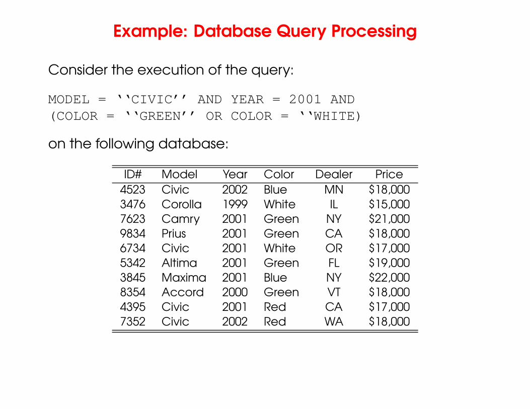
Example: Database Query Processing
Consider the execution of the query:
MODEL = ‘‘CIVIC’’ AND YEAR = 2001 AND(COLOR = ‘‘GREEN’’ OR COLOR = ‘‘WHITE)
on the following database:
ID# Model Year Color Dealer Price4523 Civic 2002 Blue MN $18,0003476 Corolla 1999 White IL $15,0007623 Camry 2001 Green NY $21,0009834 Prius 2001 Green CA $18,0006734 Civic 2001 White OR $17,0005342 Altima 2001 Green FL $19,0003845 Maxima 2001 Blue NY $22,0008354 Accord 2000 Green VT $18,0004395 Civic 2001 Red CA $17,0007352 Civic 2002 Red WA $18,000
– Typeset by FoilTEX – 5
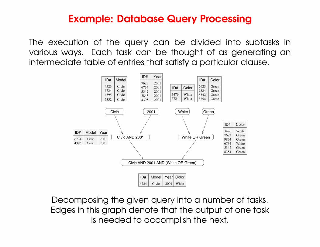
Example: Database Query Processing
The execution of the query can be divided into subtasks invarious ways. Each task can be thought of as generating anintermediate table of entries that satisfy a particular clause.
Civic AND 2001 AND (White OR Green)
White OR Green
2001Civic
Civic AND 2001
White Green
6734
ID# Model Year Color
67344395
ID# Model Year
43953845534267347623
ID# Year
4523673443957352
ID# Model
CivicCivicCivicCivic
20012001200120012001
CivicCivic
20012001
34766734
ColorID# 7623983453428354
ID# Color
347676239834673453428354
ID# Color
Civic 2001 White
GreenGreenWhiteGreenGreenWhite
WhiteWhite
GreenGreenGreenGreen
Decomposing the given query into a number of tasks.Edges in this graph denote that the output of one task
is needed to accomplish the next.
– Typeset by FoilTEX – 6

Example: Database Query Processing
Note that the same problem can be decomposed into subtasksin other ways as well.
2001 AND (White or Green)
Green
Civic AND 2001 AND (White OR Green)
Civic 2001 White
White OR Green
7623
6734 Civic White
ID# Model Year Color
2001
34766734
WhiteWhite
ColorID#
347676239834673453428354
8354
GreenGreenWhiteGreenGreenWhite
ID# Color
GreenGreen
43953845534267347623
ID# Year
20012001200120012001
20017623 Green20016734 White
Green
ID# YearColor
2001Green5342
Green
ID# Color
4523673443957352
CivicCivicCivicCivic
ID# Model
53429834
An alternate decomposition of the given problem intosubtasks, along with their data dependencies.
Different task decompositions may lead to significant differenceswith respect to their eventual parallel performance.
– Typeset by FoilTEX – 7
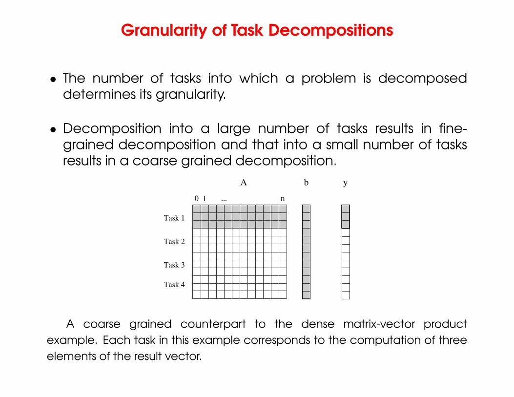
Granularity of Task Decompositions
• The number of tasks into which a problem is decomposeddetermines its granularity.
• Decomposition into a large number of tasks results in fine-grained decomposition and that into a small number of tasksresults in a coarse grained decomposition.
n10
A yb
...
Task 4
Task 2
Task 3
Task 1
A coarse grained counterpart to the dense matrix-vector productexample. Each task in this example corresponds to the computation of threeelements of the result vector.
– Typeset by FoilTEX – 8
Degree of Concurrency
• The number of tasks that can be executed in parallel is thedegree of concurrency of a decomposition.
• Since the number of tasks that can be executed in parallelmay change over program execution, the maximum degreeof concurrency is the maximum number of such tasks at anypoint during execution. What is the maximum degree ofconcurrency of the database query examples?
• The average degree of concurrency is the average numberof tasks that can be processed in parallel over the executionof the program. Assuming that each tasks in the databaseexample takes identical processing time, what is the averagedegree of concurrency in each decomposition?
• The degree of concurrency increases as the decompositionbecomes finer in granularity and vice versa.
– Typeset by FoilTEX – 9
Critical Path Length
• A directed path in the task dependency graph represents asequence of tasks that must be processed one after the other.
• The longest such path determines the shortest time in which theprogram can be executed in parallel.
• The length of the longest path in a task dependency graph iscalled the critical path length.
– Typeset by FoilTEX – 10
Critical Path Length
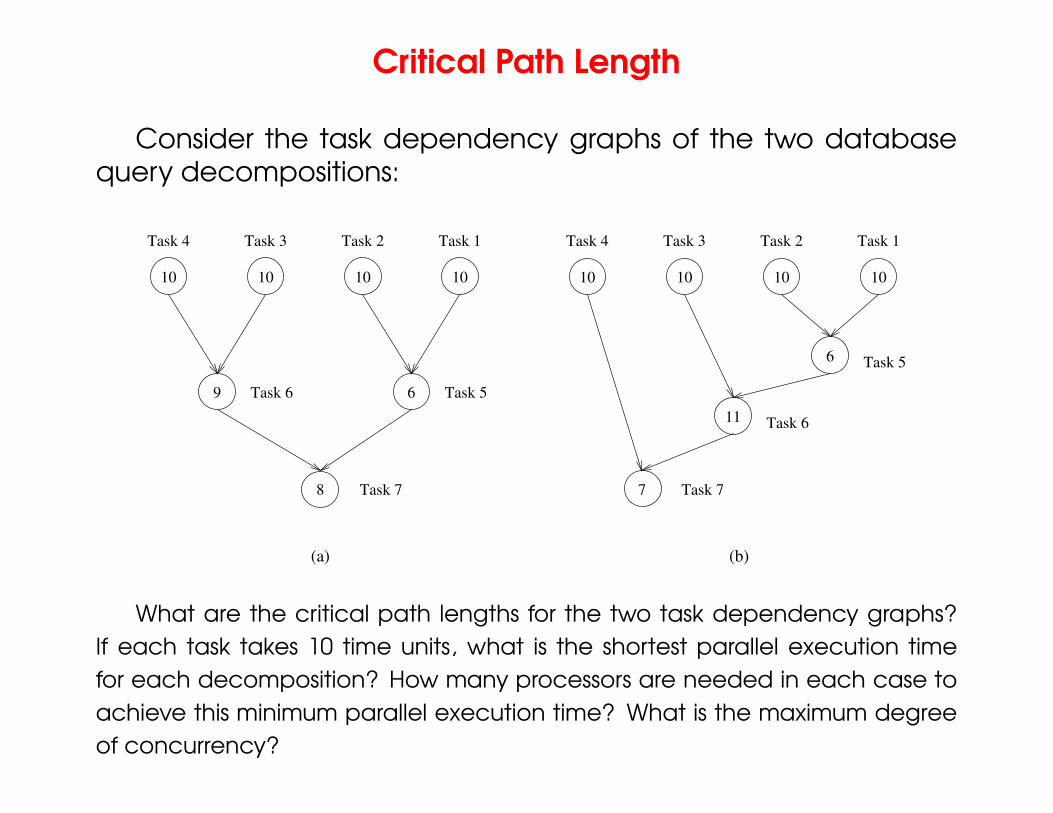
Consider the task dependency graphs of the two databasequery decompositions:
10 10 10
Task 7
10
6
7
10 10 10 10
8
9 6
11
(a) (b)
Task 1Task 1Task 2Task 3Task 4
Task 5Task 6
Task 7
Task 2Task 3Task 4
Task 5
Task 6
What are the critical path lengths for the two task dependency graphs?If each task takes 10 time units, what is the shortest parallel execution timefor each decomposition? How many processors are needed in each case toachieve this minimum parallel execution time? What is the maximum degreeof concurrency?
– Typeset by FoilTEX – 11
Limits on Parallel Performance
• It would appear that the parallel time can be made arbitrarilysmall by making the decomposition finer in granularity.
• There is an inherent bound on how fine the granularity of acomputation can be. For example, in the case of multiplyinga dense matrix with a vector, there can be no more than (n2)concurrent tasks.
• Concurrent tasks may also have to exchange data with othertasks. This results in communication overhead. The tradeoffbetween the granularity of a decomposition and associatedoverheads often determines performance bounds.
– Typeset by FoilTEX – 12
Task Interaction Graphs
• Subtasks generally exchange data with others in a decomposition.For example, even in the trivial decomposition of the densematrix-vector product, if the vector is not replicated across alltasks, they will have to communicate elements of the vector.
• The graph of tasks (nodes) and their interactions/dataexchange (edges) is referred to as a task interaction graph.
• Note that task interaction graphs represent data dependencies,whereas task dependency graphs represent control dependencies.
– Typeset by FoilTEX – 13
Task Interaction Graphs: An Example
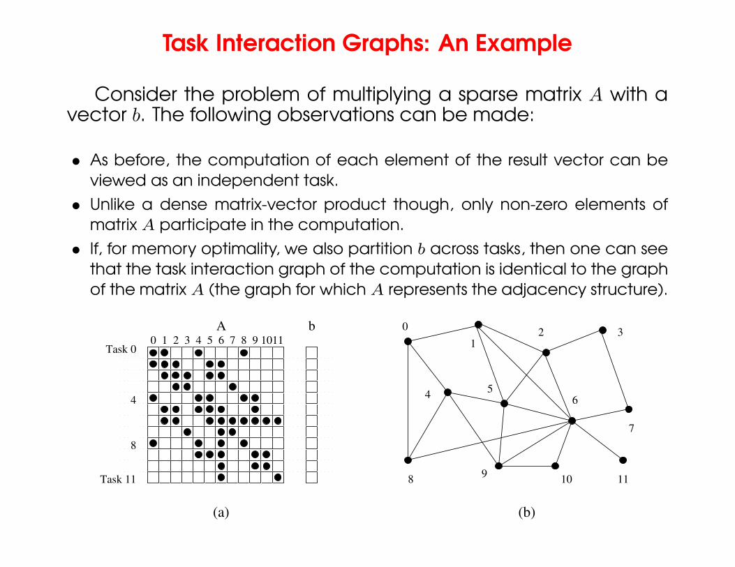
Consider the problem of multiplying a sparse matrix A with avector b. The following observations can be made:
• As before, the computation of each element of the result vector can beviewed as an independent task.
• Unlike a dense matrix-vector product though, only non-zero elements ofmatrix A participate in the computation.
• If, for memory optimality, we also partition b across tasks, then one can seethat the task interaction graph of the computation is identical to the graphof the matrix A (the graph for which A represents the adjacency structure).
4 5 6 7 8 9 10110b
21A
3
(b)
2
4 6
13
5
11109
0
8
7
Task 0
Task 11
8
4
(a)
– Typeset by FoilTEX – 14
Task Interaction Graphs, Granularity, andCommunication
In general, if the granularity of a decomposition is finer, theassociated overhead (as a ratio of useful work assocaited with atask) increases.
Example: Consider the sparse matrix-vector product examplefrom previous foil. Assume that each node takes unit time toprocess and each interaction (edge) causes an overhead of aunit time.
Viewing node 0 as an independent task involves a usefulcomputation of one time unit and overhead (communication) ofthree time units.
Now, if we consider nodes 0, 4, and 5 as one task, thenthe task has useful computation totaling to three time units andcommunication corresponding to four time units (four edges).Clearly, this is a more favorable ratio than the former case.
– Typeset by FoilTEX – 15
Processes and Mapping
• In general, the number of tasks in a decomposition exceedsthe number of processing elements available.
• For this reason, a parallel algorithm must also provide amapping of tasks to processes.
Note: We refer to the mapping as being from tasks to processes, as opposedto processors. This is because typical programming APIs, as we shall see, donot allow easy binding of tasks to physical processors. Rather, we aggregatetasks into processes and rely on the system to map these processes to physicalprocessors. We use processes, not in the UNIX sense of a process, rather, simplyas a collection of tasks and associated data.
– Typeset by FoilTEX – 16
Processes and Mapping
• Appropriate mapping of tasks to processes is critical to theparallel performance of an algorithm.
• Mappings are determined by both the task dependency andtask interaction graphs.
• Task dependency graphs can be used to ensure that workis equally spread across all processes at any point (minimumidling and optimal load balance).
• Task interaction graphs can be used to make sure thatprocesses need minimum interaction with other processes(minimum communication).
– Typeset by FoilTEX – 17
Processes and Mapping
An appropriate mapping must minimize parallel execution timeby:
• Mapping independent tasks to different processes.
• Assigning tasks on critical path to processes as soon as theybecome available.
• Minimizing interaction between processes by mapping taskswith dense interactions to the same process.
Note: These criteria often conflict eith each other. For example,a decomposition into one task (or no decomposition at all)minimizes interaction but does not result in a speedup at all! Canyou think of other such conflicting cases?
– Typeset by FoilTEX – 18
Processes and Mapping: Example
0P1P2P3
P0P0
P0P2P0
P0
P1
10 10 10 10
6
7
10 10 10 10
8
9 6
11
(a) (b)
Task 1Task 1Task 2Task 3Task 4
Task 5Task 6
Task 7
Task 2Task 3Task 4
Task 5
Task 6
Task 7
P P P P03 2
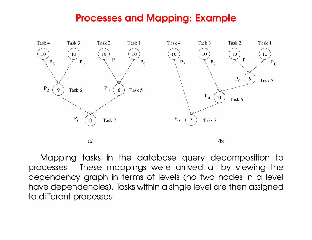
Mapping tasks in the database query decomposition toprocesses. These mappings were arrived at by viewing thedependency graph in terms of levels (no two nodes in a levelhave dependencies). Tasks within a single level are then assignedto different processes.
– Typeset by FoilTEX – 19
Decomposition Techniques
So how does one decompose a task into various subtasks?
While there is no single recipe that works for all problems, wepresent a set of commonly used techniques that apply to broadclasses of problems. These include:
• recursive decomposition
• data decomposition
• exploratory decomposition
• speculative decomposition
– Typeset by FoilTEX – 20
Recursive Decomposition
• Generally suited to problems that are solved using the divide-and-conquer strategy.
• A given problem is first decomposed into a set of sub-problems.
• These sub-problems are recursively decomposed further until adesired granularity is reached.
– Typeset by FoilTEX – 21
Recursive Decomposition: Example
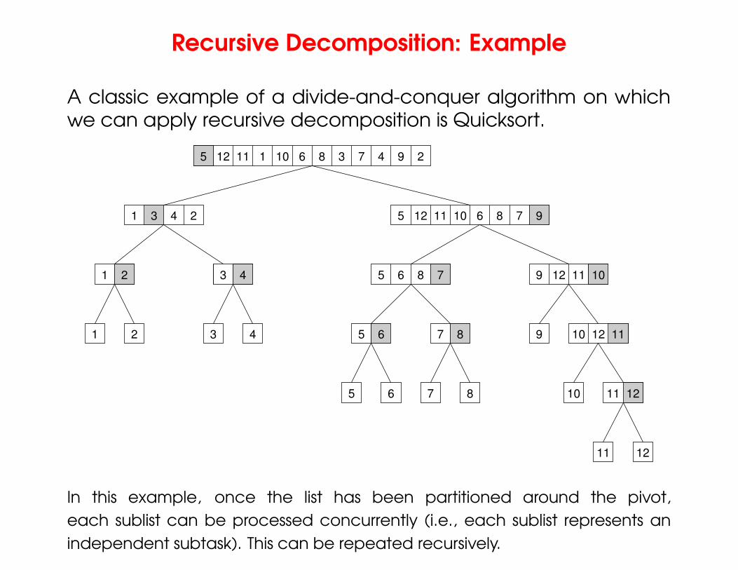
A classic example of a divide-and-conquer algorithm on whichwe can apply recursive decomposition is Quicksort.
11 12
10
9
65 87
3 421
1
11
2
1 3 4 2
3 4
865 1 311 47 2912 10
11 6 8 7 95 12 10
6 8 75
875 6 10 12 11
119 12 10
12
In this example, once the list has been partitioned around the pivot,each sublist can be processed concurrently (i.e., each sublist represents anindependent subtask). This can be repeated recursively.
– Typeset by FoilTEX – 22
Recursive Decomposition: Example
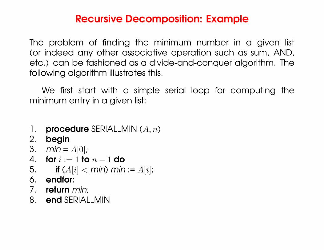
The problem of finding the minimum number in a given list(or indeed any other associative operation such as sum, AND,etc.) can be fashioned as a divide-and-conquer algorithm. Thefollowing algorithm illustrates this.
We first start with a simple serial loop for computing theminimum entry in a given list:
1. procedure SERIAL MIN (A,n)2. begin3. min = A[0];4. for i := 1 to n − 1 do5. if (A[i] < min) min := A[i];6. endfor;7. return min;8. end SERIAL MIN
– Typeset by FoilTEX – 23
Recursive Decomposition: Example
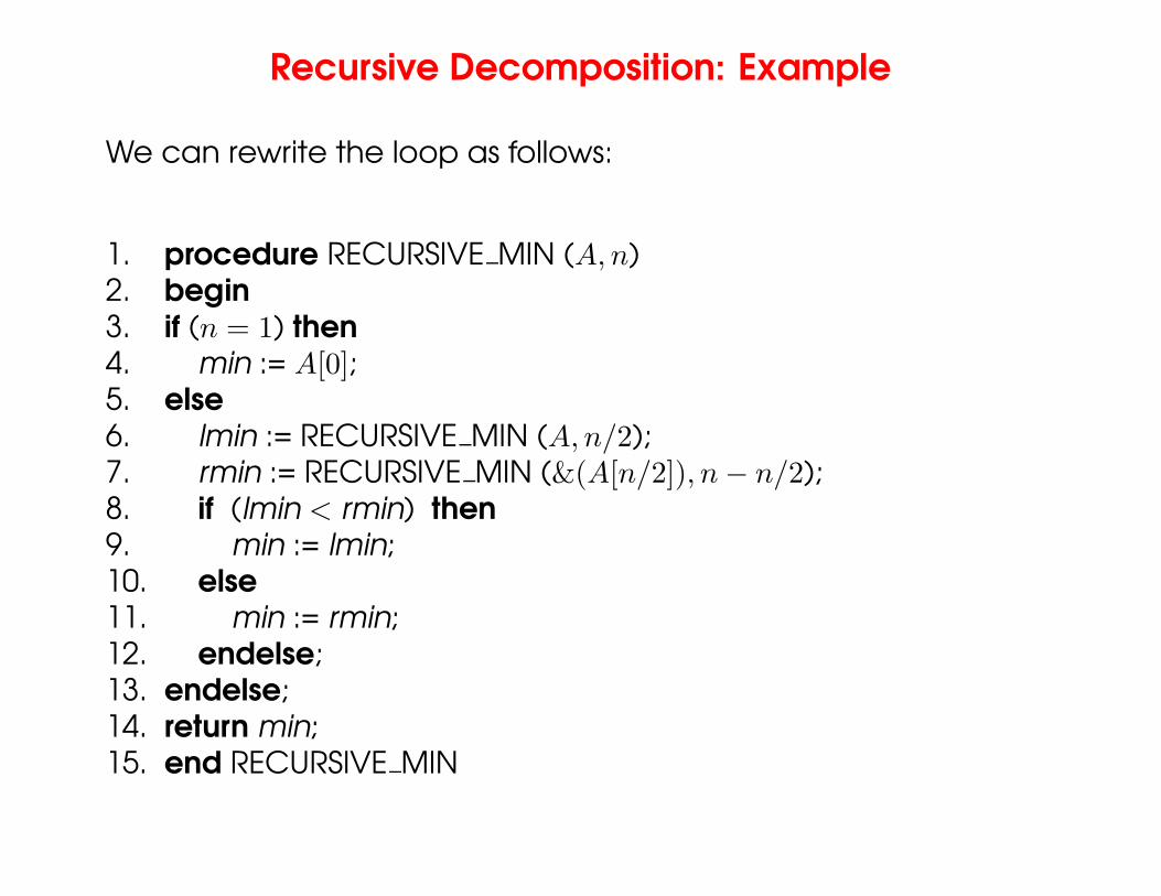
We can rewrite the loop as follows:
1. procedure RECURSIVE MIN (A,n)2. begin3. if (n = 1) then4. min := A[0];5. else6. lmin := RECURSIVE MIN (A,n/2);7. rmin := RECURSIVE MIN (&(A[n/2]), n − n/2);8. if (lmin < rmin) then9. min := lmin;10. else11. min := rmin;12. endelse;13. endelse;14. return min;15. end RECURSIVE MIN
– Typeset by FoilTEX – 24
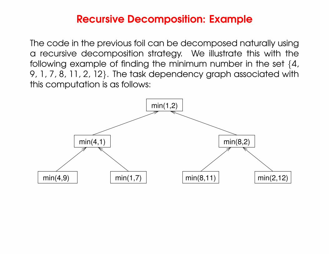
Recursive Decomposition: Example
The code in the previous foil can be decomposed naturally usinga recursive decomposition strategy. We illustrate this with thefollowing example of finding the minimum number in the set {4,9, 1, 7, 8, 11, 2, 12}. The task dependency graph associated withthis computation is as follows:
min(1,7) min(8,11)min(4,9) min(2,12)
min(1,2)
min(4,1) min(8,2)
– Typeset by FoilTEX – 25
Data Decomposition
• Identify the data on which computations are performed.
• Partition this data across various tasks.
• This partitioning induces a decomposition of the problem.
• Data can be partitioned in various ways – this critically impactsperformance of a parallel algorithm.
– Typeset by FoilTEX – 26
Data Decomposition: Output Data Decomposition
• Often, each element of the output can be computedindependently of others (but simply as a function of the input).
• A partition of the output across tasks decomposes the problemnaturally.
– Typeset by FoilTEX – 27
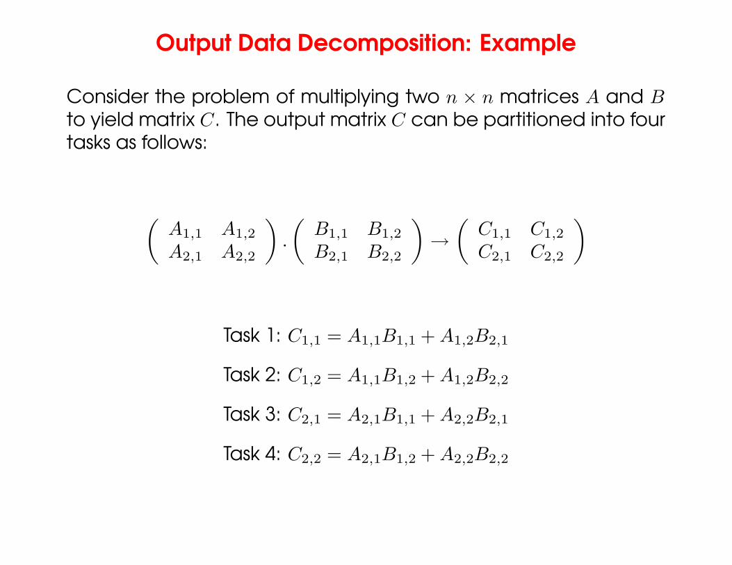
Output Data Decomposition: Example
Consider the problem of multiplying two n × n matrices A and Bto yield matrix C. The output matrix C can be partitioned into fourtasks as follows:
(
A1,1 A1,2
A2,1 A2,2
)
.
(
B1,1 B1,2
B2,1 B2,2
)
→
(
C1,1 C1,2
C2,1 C2,2
)
Task 1: C1,1 = A1,1B1,1 + A1,2B2,1
Task 2: C1,2 = A1,1B1,2 + A1,2B2,2
Task 3: C2,1 = A2,1B1,1 + A2,2B2,1
Task 4: C2,2 = A2,1B1,2 + A2,2B2,2
– Typeset by FoilTEX – 28
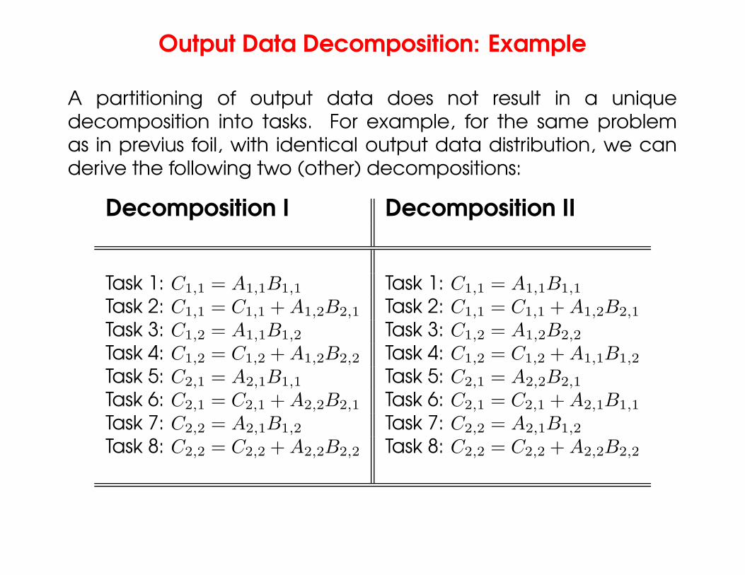
Output Data Decomposition: Example
A partitioning of output data does not result in a uniquedecomposition into tasks. For example, for the same problemas in previus foil, with identical output data distribution, we canderive the following two (other) decompositions:
Decomposition I Decomposition II
Task 1: C1,1 = A1,1B1,1 Task 1: C1,1 = A1,1B1,1
Task 2: C1,1 = C1,1 + A1,2B2,1 Task 2: C1,1 = C1,1 + A1,2B2,1
Task 3: C1,2 = A1,1B1,2 Task 3: C1,2 = A1,2B2,2
Task 4: C1,2 = C1,2 + A1,2B2,2 Task 4: C1,2 = C1,2 + A1,1B1,2
Task 5: C2,1 = A2,1B1,1 Task 5: C2,1 = A2,2B2,1
Task 6: C2,1 = C2,1 + A2,2B2,1 Task 6: C2,1 = C2,1 + A2,1B1,1
Task 7: C2,2 = A2,1B1,2 Task 7: C2,2 = A2,1B1,2
Task 8: C2,2 = C2,2 + A2,2B2,2 Task 8: C2,2 = C2,2 + A2,2B2,2
– Typeset by FoilTEX – 29
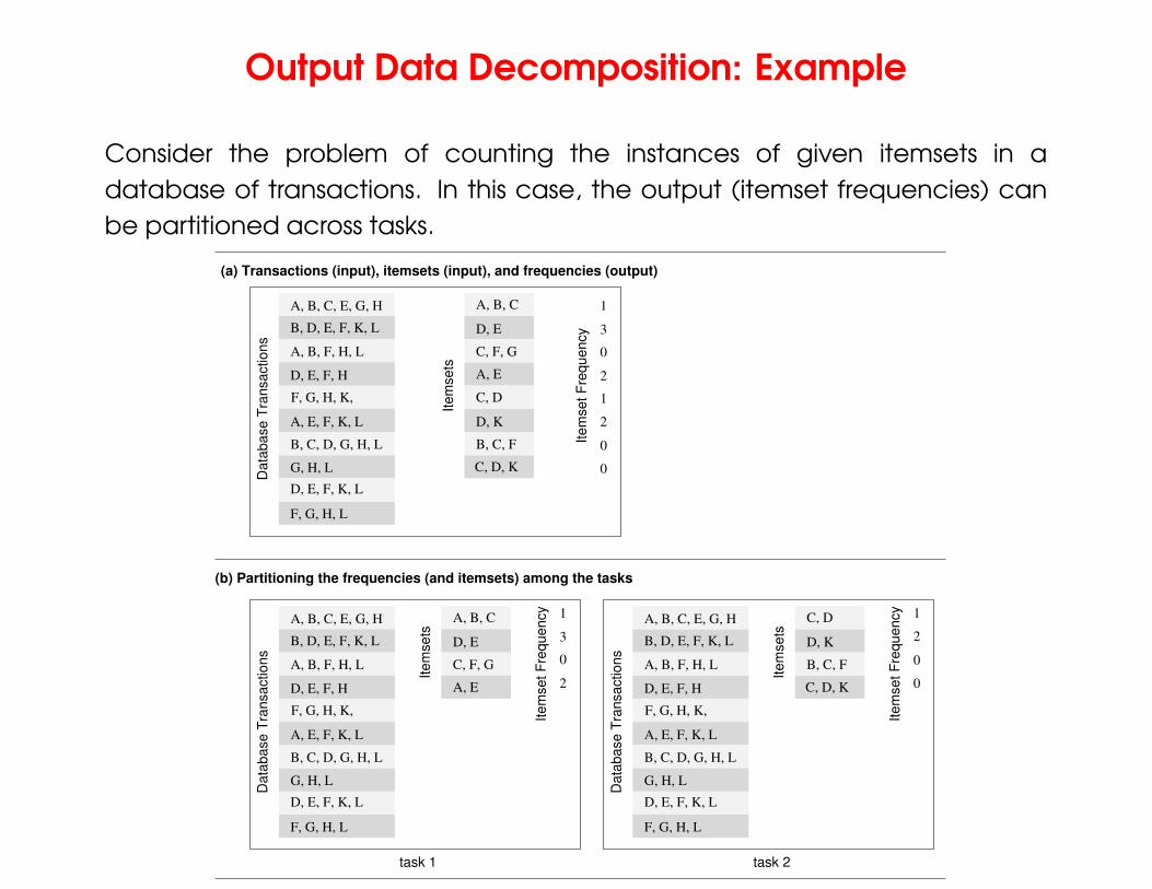
Output Data Decomposition: Example
Consider the problem of counting the instances of given itemsets in adatabase of transactions. In this case, the output (itemset frequencies) canbe partitioned across tasks.
Item
sets
Dat
abas
e T
rans
actio
ns
Item
set F
requ
ency
Item
set F
requ
ency
Item
sets
Item
set F
requ
ency
Dat
abas
e T
rans
actio
ns
Dat
abas
e T
rans
actio
ns
Item
sets
0
0
A, B, C, E, G, H
A, E, F, K, L
B, D, E, F, K, L
A, B, F, H, L
D, E, F, H
2
F, G, H, K,
(b) Partitioning the frequencies (and itemsets) among the tasks
B, C, D, G, H, L
D, E, F, K, L
F, G, H, L
G, H, L
A, B, C
D, E
A, B, C, E, G, H
A, E, F, K, L
D, K
C, D, K
B, C, F
C, D2
0
0
1
B, D, E, F, K, L
A, B, F, H, L
D, E, F, H
task 2
F, G, H, K,
B, C, D, G, H, L
D, E, F, K, L
F, G, H, L
G, H, L
C, F, G
C, D
B, C, F
C, D, K
A, B, C, E, G, H
A, E, F, K, L
B, D, E, F, K, L
A, B, F, H, L
D, E, F, H
F, G, H, K,
B, C, D, G, H, L
D, E, F, K, L
F, G, H, L
G, H, L
A, E
D, K
1
3
A, E
C, F, G
D, E
A, B, C
2
0
3
1
0
2
1
task 1
(a) Transactions (input), itemsets (input), and frequencies (output)
– Typeset by FoilTEX – 30
Output Data Decomposition: Example
From the previous example, the following observations can bemade:
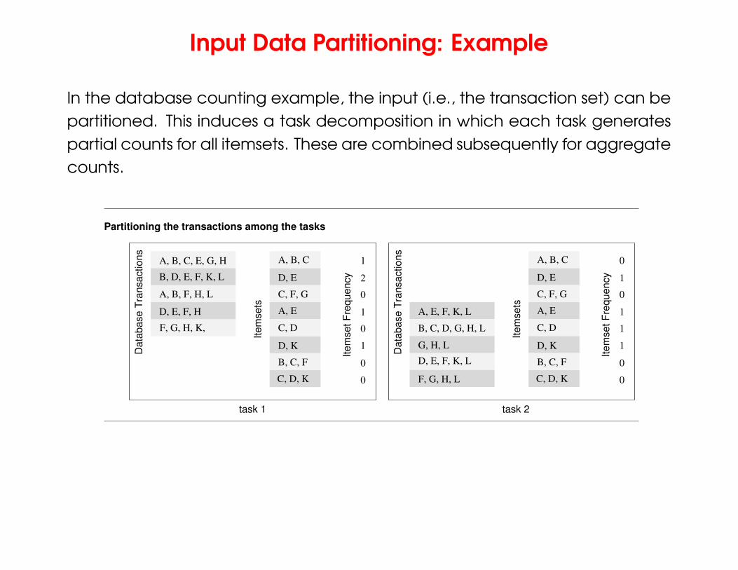
• If the database of transactions is replicated across theprocesses, each task can be independently accomplishedwith no communication.
• If the database is partitioned across processes as well (forreasons of memory utilization), each task first computes partialcounts. These counts are then aggregated at the appropriatetask.
– Typeset by FoilTEX – 31
Input Data Partitioning
• Generally applicable if each output can be naturallycomputed as a function of the input.
• In many cases, this is the only natural decomposition becausethe output is not clearly known a-priori (e.g., the problem offinding the minimum in a list, sorting a given list, etc.).
• A task is associated with each input data partition. The taskperforms as much of the computation with its part of the data.Subsequent processing combines these partial results.
– Typeset by FoilTEX – 32
Input Data Partitioning: Example
In the database counting example, the input (i.e., the transaction set) can bepartitioned. This induces a task decomposition in which each task generatespartial counts for all itemsets. These are combined subsequently for aggregatecounts.
Item
set F
requ
ency
Dat
abas
e T
rans
actio
ns
Item
sets
Item
set F
requ
ency
Dat
abas
e T
rans
actio
ns
Item
sets
D, K
A, E
C, D, K
B, C, F
C, D
C, F, G
D, E
A, B, C
C, F, G
1
0
0
1
1
0
1
0
task 2
D, E
A, B, C
Partitioning the transactions among the tasks
A, B, C, E, G, H
0
2
1
1
0
task 1
C, D
B, C, F
C, D, K
A, E
D, K
A, E, F, K, L
B, C, D, G, H, L
D, E, F, K, L
F, G, H, L
G, H, L
0
0
1
F, G, H, K,
D, E, F, H
A, B, F, H, L
B, D, E, F, K, L
– Typeset by FoilTEX – 33
Partitioning Input and Output Data
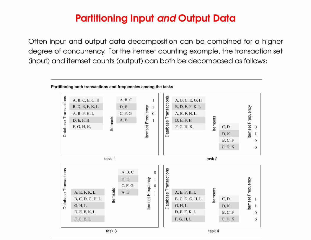
Often input and output data decomposition can be combined for a higherdegree of concurrency. For the itemset counting example, the transaction set(input) and itemset counts (output) can both be decomposed as follows:
Item
sets
Dat
abas
e T
rans
actio
ns
Item
set F
requ
ency
Dat
abas
e T
rans
actio
ns
Item
sets
Item
set F
requ
ency
Dat
abas
e T
rans
actio
ns
Item
set F
requ
ency
Item
sets
Item
set F
requ
ency
Item
sets
Dat
abas
e T
rans
actio
ns
B, D, E, F, K, L
A, B, C, E, G, H
D, K
A, E, F, K, L
B, C, D, G, H, L
D, E, F, K, L
F, G, H, L
G, H, L 1
Partitioning both transactions and frequencies among the tasks
task 4task 3
0
1
0
1
1
0
0
C, D
B, C, F
C, D, K
D, E, F, K, L
B, C, F
C, D, K
D, K
A, E
C, F, G
D, E
A, B, C
F, G, H, K,
D, E, F, H
A, B, F, H, L
B, D, E, F, K, L
A, B, C, E, G, H
1
0
2
1
task 1
C, D
A, B, F, H, L
D, E, F, H
G, H, L
F, G, H, L
B, C, D, G, H, L
A, E, F, K, L
F, G, H, K,
A, B, C
D, E
C, F, G
A, E
task 2
0
0
0
1
– Typeset by FoilTEX – 34
Intermediate Data Partitioning
• Computation can often be viewed as a sequence oftransformation from the input to the output data.
• In these cases, it is often beneficial to use one of theintermediate stages as a basis for decomposition.
– Typeset by FoilTEX – 35
Intermediate Data Partitioning: Example
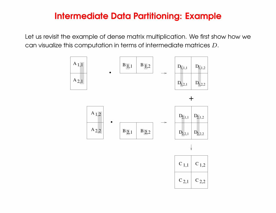
Let us revisit the example of dense matrix multiplication. We first show how wecan visualize this computation in terms of intermediate matrices D.
1,1 1,2BB
1,1C
D
DD
D
D
D
D
D1,1,1
A 2,1
1,1A
2,2
A 1,2
A B 2,22,1B
.
.
+
2,1,1
1,1,2
1,2,1 1,2,2
2,1,2
2,2,1
C C
C 1,2
2,1 2,2
2,2,2
– Typeset by FoilTEX – 36
Intermediate Data Partitioning: Example
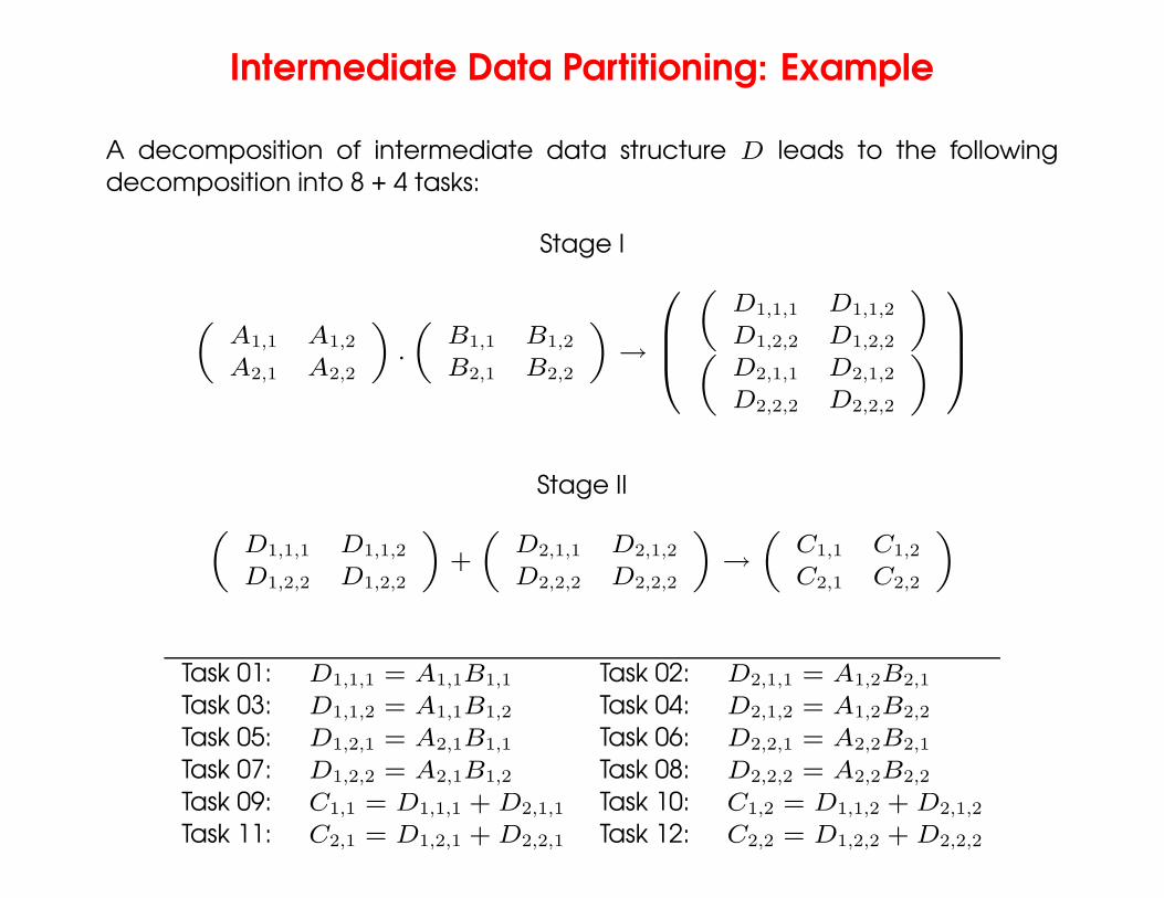
A decomposition of intermediate data structure D leads to the followingdecomposition into 8 + 4 tasks:
Stage I
„
A1,1 A1,2
A2,1 A2,2
«
.
„
B1,1 B1,2
B2,1 B2,2
«
→
0
B
B
@
„
D1,1,1 D1,1,2
D1,2,2 D1,2,2
«
„
D2,1,1 D2,1,2
D2,2,2 D2,2,2
«
1
C
C
A
Stage II
„
D1,1,1 D1,1,2
D1,2,2 D1,2,2
«
+
„
D2,1,1 D2,1,2
D2,2,2 D2,2,2
«
→
„
C1,1 C1,2
C2,1 C2,2
«
Task 01: D1,1,1 = A1,1B1,1 Task 02: D2,1,1 = A1,2B2,1
Task 03: D1,1,2 = A1,1B1,2 Task 04: D2,1,2 = A1,2B2,2
Task 05: D1,2,1 = A2,1B1,1 Task 06: D2,2,1 = A2,2B2,1
Task 07: D1,2,2 = A2,1B1,2 Task 08: D2,2,2 = A2,2B2,2
Task 09: C1,1 = D1,1,1 + D2,1,1 Task 10: C1,2 = D1,1,2 + D2,1,2
Task 11: C2,1 = D1,2,1 + D2,2,1 Task 12: C2,2 = D1,2,2 + D2,2,2
– Typeset by FoilTEX – 37
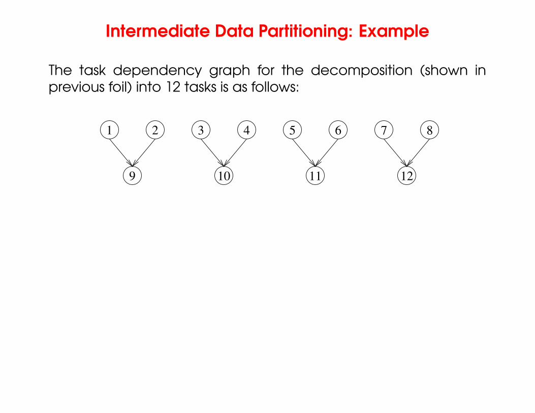
Intermediate Data Partitioning: Example
The task dependency graph for the decomposition (shown inprevious foil) into 12 tasks is as follows:
1
12
3 42 5 6 7 8
9 10 11
– Typeset by FoilTEX – 38
The Owner Computes Rule
• The Owner Computes Rule generally states that the processassined a particular data item is responsible for all computationassociated with it.
• In the case of input data decomposition, the owner computesrule imples that all computations that use the input data areperformed by the process.
• In the case of output data decomposition, the ownercomputes rule implies that the output is computed by theprocess to which the output data is assigned.
– Typeset by FoilTEX – 39
Exploratory Decomposition
• In many cases, the decomposition of the problem goes hand-in-hand with its execution.
• These problems typically involve the exploration (search) of astate space of solutions.
• Problems in this class include a variety of discrete optimizationproblems (0/1 integer programming, QAP, etc.), theoremproving, game playing, etc.
– Typeset by FoilTEX – 40
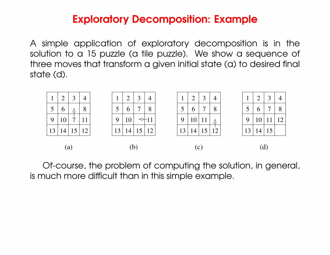
Exploratory Decomposition: Example
A simple application of exploratory decomposition is in thesolution to a 15 puzzle (a tile puzzle). We show a sequence ofthree moves that transform a given initial state (a) to desired finalstate (d).
1 2 3 4
5 6 8
9 10
13 14 15 12
117
1 2 3 4
5 6 7 8
9 10
13 14 15 12
11
(d)
1 2 3 4
5 6 7 8
9 10 11
13 14 15 12
1 2 3 4
5 6 7 8
9 10 11 12
13 14 15
(a) (b) (c)
Of-course, the problem of computing the solution, in general,is much more difficult than in this simple example.
– Typeset by FoilTEX – 41
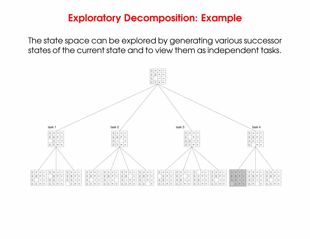
Exploratory Decomposition: Example
The state space can be explored by generating various successorstates of the current state and to view them as independent tasks.
12
34
56
78
910
1314
1512 11
12
34
56
8
910
1314
1512 11
71
24
56
8
910
1314
1512 11
7 3
12
34
58
910
1314
1512 11
7 6
12
34
56
910
1314
1512 11
7 8
12
34
56
8
910
1314
1512 11
7
12
34
56
78
91314
1512 11
10
12
34
56
78
1314
1512 11
109
12
34
57
8
91314
1512 11
106
12
34
56
78
91315
12 1110
task 1
14
12
34
56
78
91314
1512 11
10
12
34
56
78
910
1312 11
1514
12
34
56
78
910
1314
12 1115
12
34
56
78
910
1314
111512
12
34
56
78
910
1314
12 11
15
12
34
56
78
910
1314
1512
11
12
34
56
7
910
1314
1512
118
12
34
56
78
910
1314
1512 11
task 3task 2 task 4
12
34
56
78
910
1314
15 1112
– Typeset by FoilTEX – 42
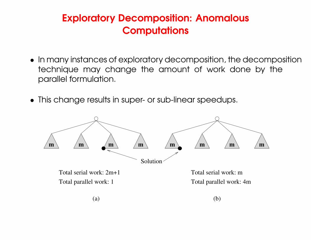
Exploratory Decomposition: AnomalousComputations
• In many instances of exploratory decomposition, the decompositiontechnique may change the amount of work done by theparallel formulation.
• This change results in super- or sub-linear speedups.
Solution
(b)
m m m m m m m m
Total serial work: 2m+1
Total parallel work: 1
Total serial work: m
Total parallel work: 4m
(a)
– Typeset by FoilTEX – 43
Speculative Decomposition
• In some applications, dependencies between tasks are notknown a-priori.
• For such applications, it is impossible to identify independenttasks.
• There are generally two approaches to dealing withsuch applications: conservative approaches, which identifyindependent tasks only when they are guaranteed to not havedependencies, and, optimistic approaches, which scheduletasks even when they may potentially be erroneous.
• Conservative approaches may yield little concurrency andoptimistic approaches may require roll-back mechanism in thecase of an error.
– Typeset by FoilTEX – 44
Speculative Decomposition: Example
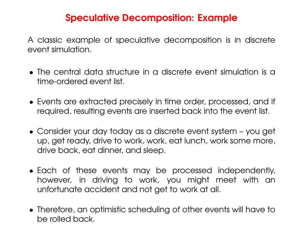
A classic example of speculative decomposition is in discreteevent simulation.
• The central data structure in a discrete event simulation is atime-ordered event list.
• Events are extracted precisely in time order, processed, and ifrequired, resulting events are inserted back into the event list.
• Consider your day today as a discrete event system – you getup, get ready, drive to work, work, eat lunch, work some more,drive back, eat dinner, and sleep.
• Each of these events may be processed independently,however, in driving to work, you might meet with anunfortunate accident and not get to work at all.
• Therefore, an optimistic scheduling of other events will have tobe rolled back.
– Typeset by FoilTEX – 45
Speculative Decomposition: Example
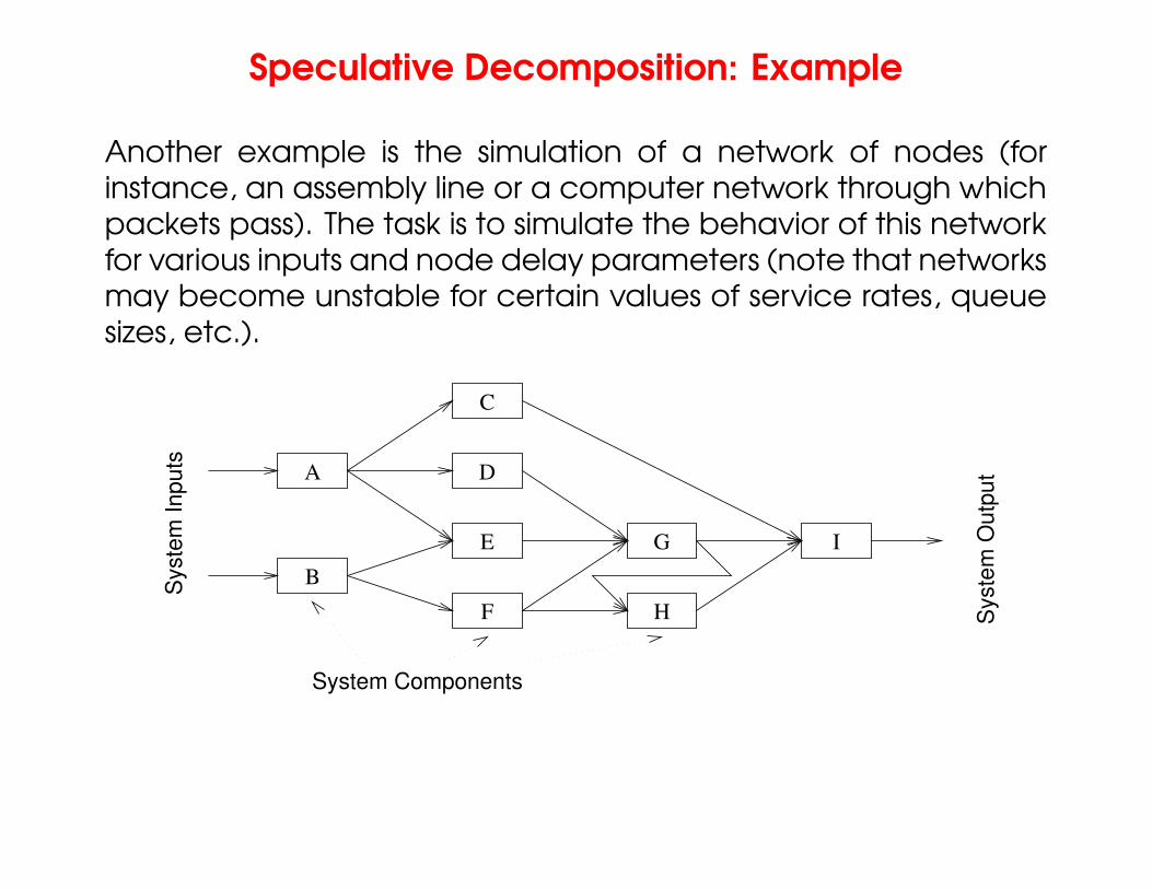
Another example is the simulation of a network of nodes (forinstance, an assembly line or a computer network through whichpackets pass). The task is to simulate the behavior of this networkfor various inputs and node delay parameters (note that networksmay become unstable for certain values of service rates, queuesizes, etc.).
System Components
A
B
C
D
E
F
G
H
I
Sys
tem
Inpu
ts
Sys
tem
Out
put
– Typeset by FoilTEX – 46
Hybrid Decompositions
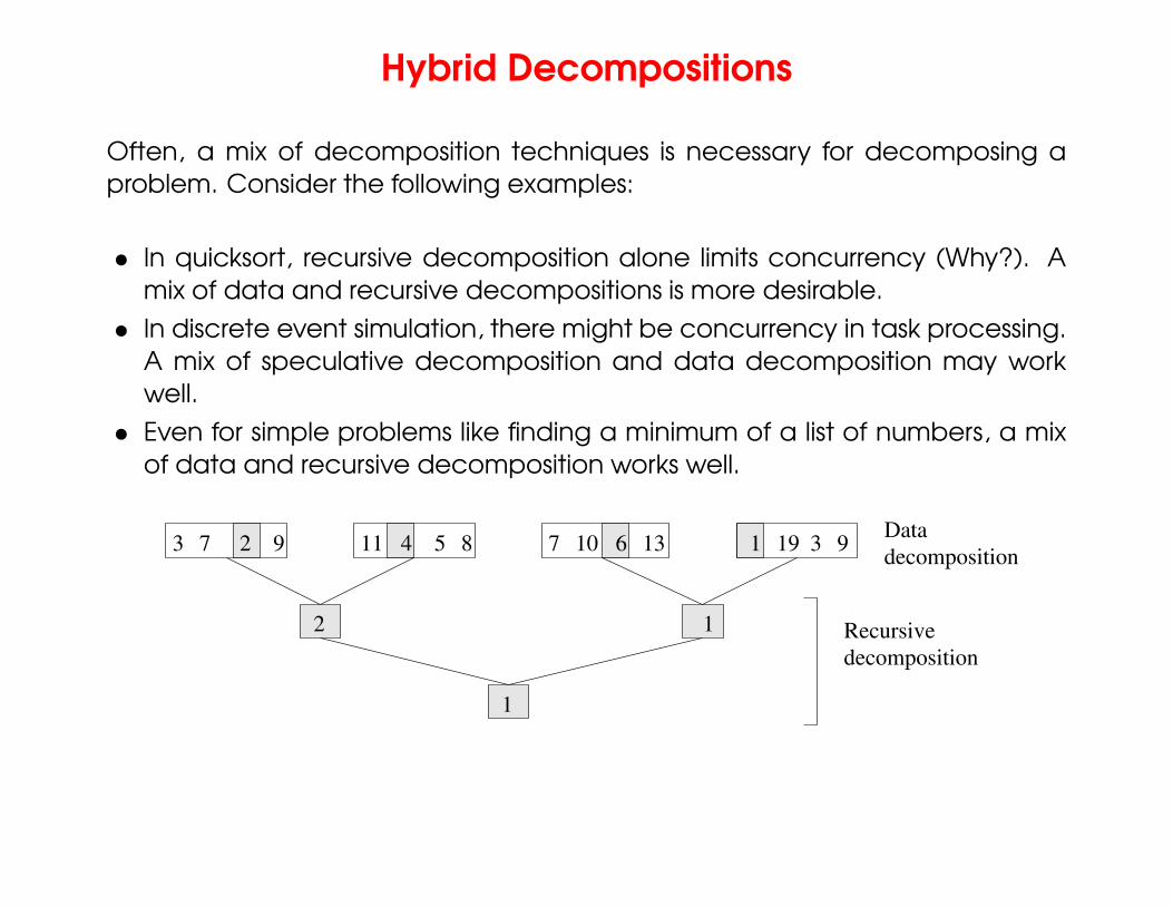
Often, a mix of decomposition techniques is necessary for decomposing aproblem. Consider the following examples:
• In quicksort, recursive decomposition alone limits concurrency (Why?). Amix of data and recursive decompositions is more desirable.
• In discrete event simulation, there might be concurrency in task processing.A mix of speculative decomposition and data decomposition may workwell.
• Even for simple problems like finding a minimum of a list of numbers, a mixof data and recursive decomposition works well.
2 1
1
1
Recursivedecomposition
Datadecomposition
3 7 2 11 75 8 10 6 13 19 3 99 4
– Typeset by FoilTEX – 47
Characteristics of Tasks
Once a problem has been decomposed into independent tasks,the characteristics of these tasks critically impact choice andperformance of parallel algorithms. Relevant task characteristicsinclude:
• Task generation.
• Task sizes.
• Size of data associated with tasks.
– Typeset by FoilTEX – 48
Task Generation
• Static task generation: Concurrent tasks can be identifieda-priori. Typical matrix operations, graph algorithms,image processing applications, and other regularly structuredproblems fall in this class. These can typically be decomposedusing data or recursive decomposition techniques.
• Dynamic task generation: Tasks are generated as we performcomputation. A classic example of this is in game playing– each 15 puzzle board is generated from the previousone. These applications are typically decomposed usingexploratory or speculative decompositions.
– Typeset by FoilTEX – 49
Task Sizes
• Task sizes may be uniform (i.e., all tasks are the same size) ornon-uniform.
• Non-uniform task sizes may be such that they can bedetermined (or estimated) a-priori or not.
• Examples in this class include discrete optimization problems, inwhich it is difficult to estimate the effective size of a state space.
– Typeset by FoilTEX – 50

Size of Data Associated with Tasks
• The size of data associated with a task may be small or largewhen viewed in the context of the size of the task.
• A small context of a task implies that an algorithm can easilycommunicate this task to other processes dynamically (e.g.,the 15 puzzle).
• A large context ties the task to a process, or alternately, analgorithm may attempt to reconstruct the context at anotherprocesses as opposed to communicating the context of thetask (e.g., 0/1 integer programming).
– Typeset by FoilTEX – 51
Characteristics of Task Interactions
Tasks may communicate with each other in various ways. Theassociated dichotomy is:
• Static interactions: The tasks and their interactions are knowna-priori. These are relatively simpler to code into programs.
• Dynamic interactions: The timing or interacting tasks cannotbe determined a-priori. These interactions are harder to code,especitally, as we shall see, using message passing APIs.
– Typeset by FoilTEX – 52
Characteristics of Task Interactions
• Regular interactions: There is a definite pattern (in the graphsense) to the interactions. These patterns can be exploited forefficient implementation.
• Irregular interactions: Interactions lack well-defined topologies.
– Typeset by FoilTEX – 53
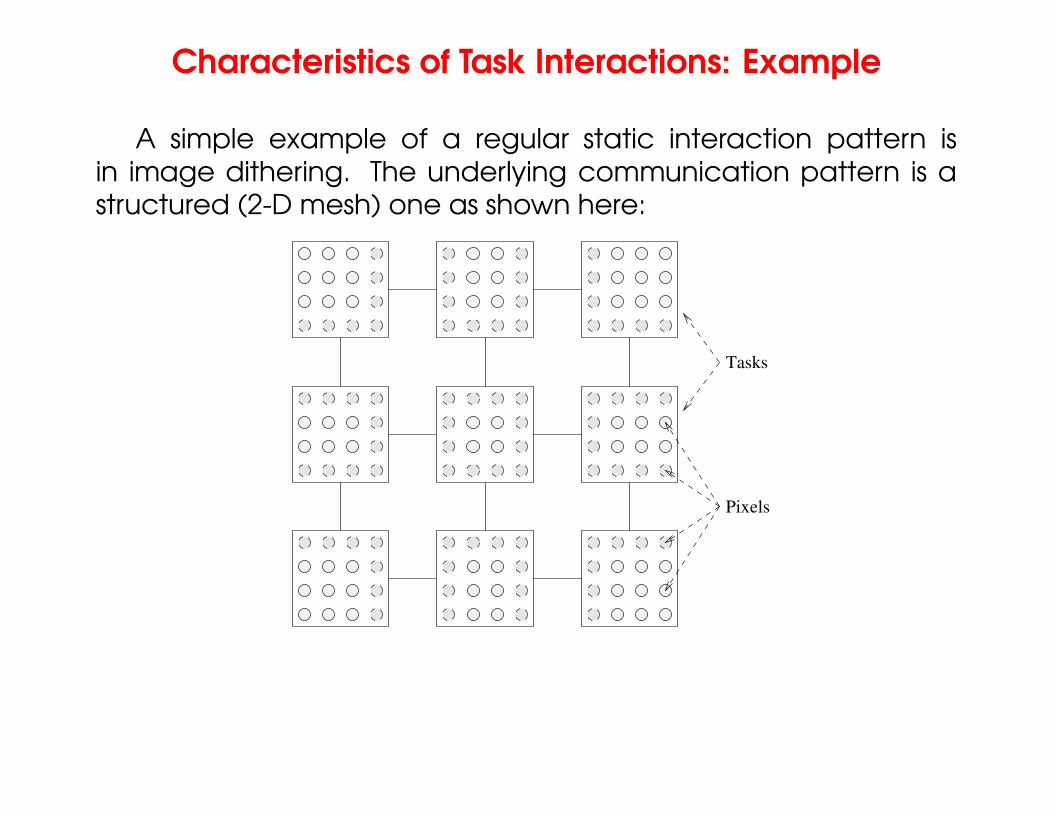
Characteristics of Task Interactions: Example
A simple example of a regular static interaction pattern isin image dithering. The underlying communication pattern is astructured (2-D mesh) one as shown here:
Pixels
Tasks
– Typeset by FoilTEX – 54
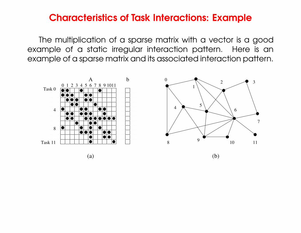
Characteristics of Task Interactions: Example
The multiplication of a sparse matrix with a vector is a goodexample of a static irregular interaction pattern. Here is anexample of a sparse matrix and its associated interaction pattern.
4 5 6 7 8 9 10110b
21A
3
(b)
2
4 6
13
5
11109
0
8
7
Task 0
Task 11
8
4
(a)
– Typeset by FoilTEX – 55
Characteristics of Task Interactions
• Interactions may be read-only or read-write.
• In read-only interactions, tasks just read data items associatedwith other tasks.
• In read-write interactions tasks read, as well as modily dataitems associated with other tasks.
• In general, read-write interactions are harder to code, sincethey require additional synchronization primitives.
– Typeset by FoilTEX – 56

Characteristics of Task Interactions
• Interactions may be one-way or two-way.
• A one-way interaction can be initiated and accomplished byone of the two interacting tasks.
• A two-way interaction requires participation from both tasksinvolved in an interaction.
• One way interactions are somewhat harder to code inmessage passing APIs.
– Typeset by FoilTEX – 57
Mapping Techniques
• Once a problem has been decomposed into concurrent tasks,these must be mapped to processes (that can be executed ona parallel platform).
• Mappings must minimize overheads.
• Primary overheads are communication and idling.
• Minimizing these overheads often represents contradictingobjectives.
• Assigning all work to one processor trivially minimizescommunication at the expense of significant idling.
– Typeset by FoilTEX – 58
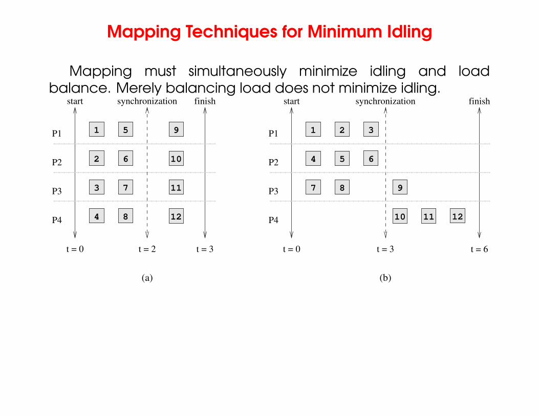
Mapping Techniques for Minimum Idling
Mapping must simultaneously minimize idling and loadbalance. Merely balancing load does not minimize idling.
12
11
10
P1 9
P2
synchronization
P3
P4
t = 0
start
1
t = 0
start
1
2
3
4
5
6
7
8
finish
t = 3
2 3
4 5 6
7 8 9
10 11 12
synchronization
t = 3
finish
t = 6
(a) (b)
P1
P2
P3
P4
t = 2
– Typeset by FoilTEX – 59

Mapping Techniques for Minimum Idling
Mapping techniques can be static or dynamic.
• Static Mapping: Tasks are mapped to processes a-priori. Forthis to work, we must have a good estimate of the size of eachtask. Even in these cases, the problem may be NP complete.
• Dynamic Mapping: Tasks are mapped to processes at runtime.This may be because the tasks are generated at runtime, orthat their sizes are not known.
Other factors that determine the choice of techniques includethe size of data associated with a task and the nature ofunderlying domain.
– Typeset by FoilTEX – 60
Schemes for Static Mapping
• Mappings based on data partitioning.
• Mappings based on task graph partitioning.
• Hybrid mappings.
– Typeset by FoilTEX – 61
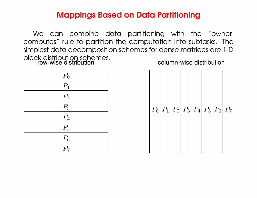
Mappings Based on Data Partitioning
We can combine data partitioning with the “owner-computes” rule to partition the computation into subtasks. Thesimplest data decomposition schemes for dense matrices are 1-Dblock distribution schemes.
column-wise distributionrow-wise distribution
PSfrag replacements
P0
P0
P1
P1
P2
P2
P3P3 P4
P4
P5
P5
P6
P6
P7
P7
P8
P9
P10
P11
P12
P13
P14
P15
– Typeset by FoilTEX – 62
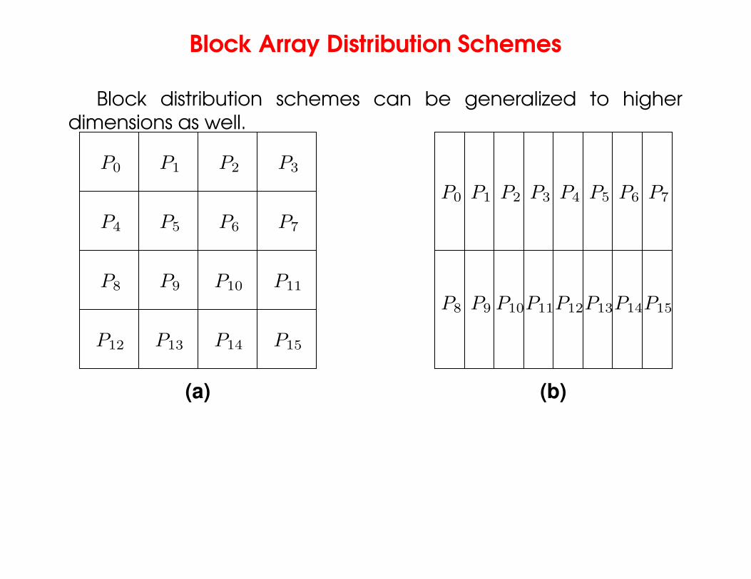
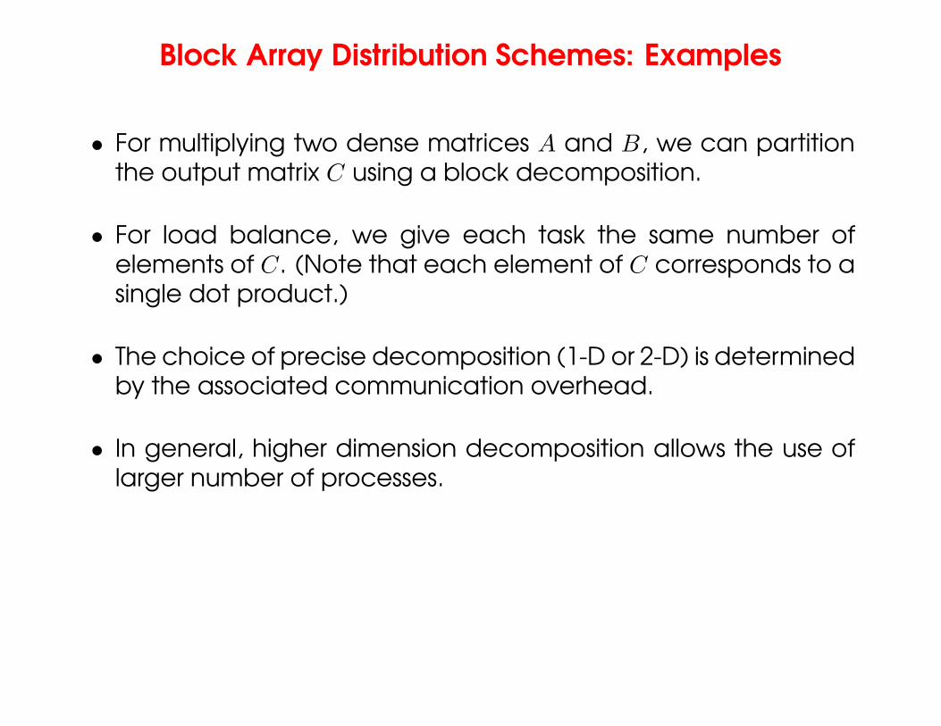
Block Array Distribution Schemes
Block distribution schemes can be generalized to higherdimensions as well.
(b)(a)
PSfrag replacements
P0
P0 P1
P1
P2
P2
P3
P3
P4
P4
P5
P5
P6
P6
P7
P7
P8
P8
P9
P9
P10
P10
P11
P11
P12
P12
P13
P13
P14
P14
P15
P15
– Typeset by FoilTEX – 63
Block Array Distribution Schemes: Examples
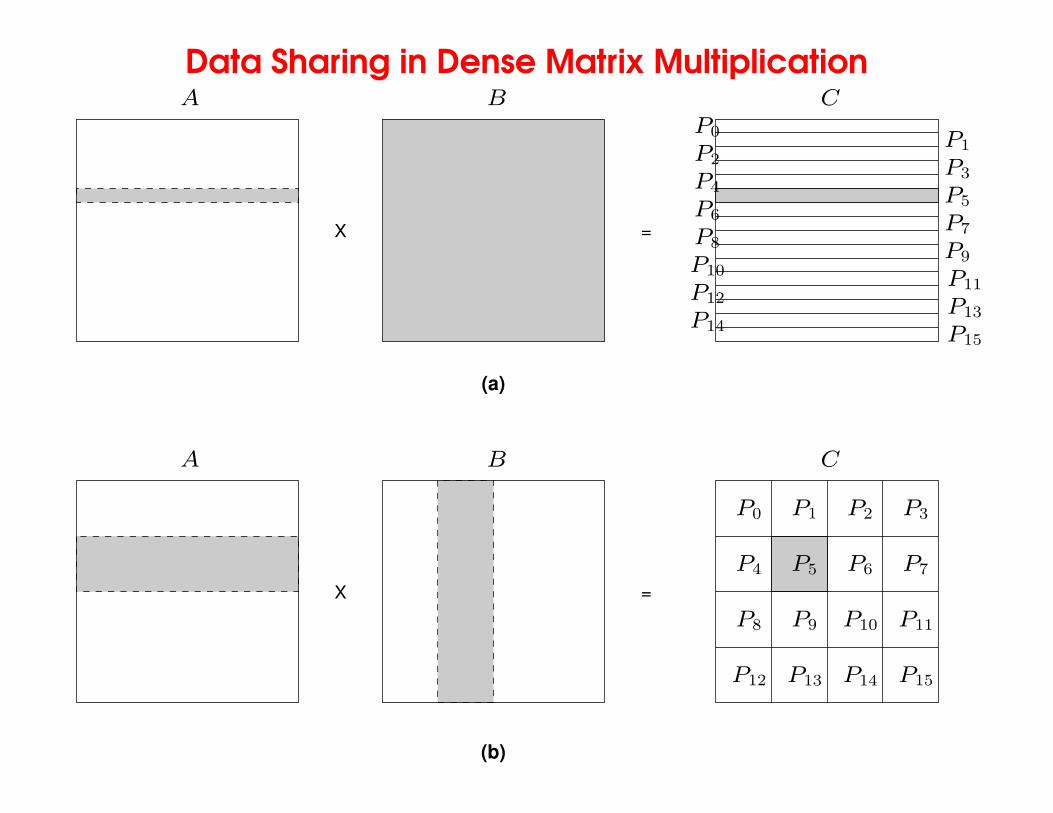
• For multiplying two dense matrices A and B, we can partitionthe output matrix C using a block decomposition.
• For load balance, we give each task the same number ofelements of C. (Note that each element of C corresponds to asingle dot product.)
• The choice of precise decomposition (1-D or 2-D) is determinedby the associated communication overhead.
• In general, higher dimension decomposition allows the use oflarger number of processes.
– Typeset by FoilTEX – 64
Data Sharing in Dense Matrix Multiplication
(a)
(b)
X
X =
=
PSfrag replacements
P0
P0
P1
P1
P2
P2
P3
P3
P4
P4
P5
P5
P6
P6
P7
P7
P8
P8
P9
P9
P10
P10
P11
P11
P12
P12
P13
P13
P14
P14
P15
P15
C
CA
A B
B
– Typeset by FoilTEX – 65
Cyclic and Block Cyclic Distributions
• If the amount of computation associated with data itemsvaries, a block decomposition may lead to significant loadimbalances.
• A simple example of this is in LU decomposition (or GaussianElimination) of dense matrices.
– Typeset by FoilTEX – 66

LU Factorization of a Dense Matrix
A decomposition of LU factorization into 14 tasks – notice thesignificant load imbalance.
A1,1 A1,2 A1,3
A2,1 A2,2 A2,3
A3,1 A3,2 A3,3
→
L1,1 0 0L2,1 L2,2 0L3,1 L3,2 L3,3
.
U1,1 U1,2 U1,3
0 U2,2 U2,3
0 0 U3,3
1: A1,1 → L1,1U1,1 6: A2,2 = A2,2 − L2,1U1,2 11: L3,2 = A3,2U−1
2,2
2: L2,1 = A2,1U−11,1 7: A3,2 = A3,2 − L3,1U1,2 12: U2,3 = L−1
2,2A2,3
3: L3,1 = A3,1U−1
1,1 8: A2,3 = A2,3 − L2,1U1,3 13: A3,3 = A3,3 − L3,2U2,3
4: U1,2 = L−11,1A1,2 9: A3,3 = A3,3 − L3,1U1,3 14: A3,3 → L3,3U3,3
5: U1,3 = L−1
1,1A1,3 10: A2,2 → L2,2U2,2
– Typeset by FoilTEX – 67
Block Cyclic Distributions
• Variation of the block distribution scheme that can be used toalleviate the load-imbalance and idling problems.
• Partition an array into many more blocks than the number ofavailable processes.
• Blocks are assigned to processes in a round-robin manner sothat each process gets several non-adjacent blocks.
– Typeset by FoilTEX – 68
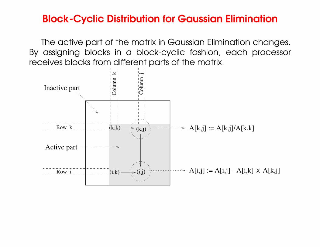
Block-Cyclic Distribution for Gaussian Elimination
The active part of the matrix in Gaussian Elimination changes.By assigning blocks in a block-cyclic fashion, each processorreceives blocks from different parts of the matrix.
A[i,j] := A[i,j] - A[i,k] A[k,j]
Row k
Row i
(k,k) (k,j)
Inactive part
Active part
A[k,j] := A[k,j]/A[k,k]
x(i,k) (i,j)
Col
umn
k
Col
umn
j
– Typeset by FoilTEX – 69
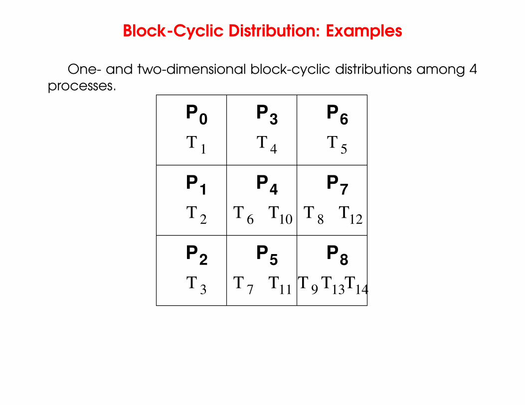
Block-Cyclic Distribution: Examples
One- and two-dimensional block-cyclic distributions among 4processes.
0 P P
PPP1
P
T T
P
T T T
P
T
TTT
P
T
14
T
T T T6
2
3
4
5
7
8
1
2
3
4 5
6 10
7
8
911
12
13
– Typeset by FoilTEX – 70

Block-Cyclic Distribution
• A cyclic distribution is a special case in which block size is one.
• A block distribution is a special case in which block size is n/p,where n is the dimension of the matrix and p is the number ofprocesses.
(b)(a)
PSfrag replacements
P0
P0P0 P0
P0P0P1
P1
P1
P1
P1
P1
P2
P2P2
P2
P2
P2
P3
P3P3
P3
P3 P3
P4
P5
P6
P7
P8
P9
P10
P11
P12
P13
P14
P15
– Typeset by FoilTEX – 71
Graph Partitioning Dased Data Decomposition
• In case of sparse matrices, block decompositions are morecomplex.
• Consider the problem of multiplying a sparse matrix with avector.
• The graph of the matrix is a useful indicator of the work (numberof nodes) and communication (the degree of each node).
• In this case, we would like to partition the graph so as to assignequal number of nodes to each process, while minimizingedge count of the graph partition.
– Typeset by FoilTEX – 72
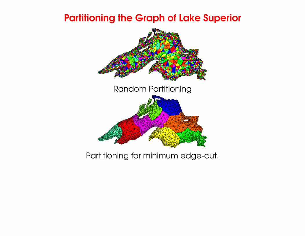
Partitioning the Graph of Lake Superior
Random Partitioning
Partitioning for minimum edge-cut.
– Typeset by FoilTEX – 73

Mappings Based on Task Paritioning
• Partitioning a given task-dependency graph across processes.
• Determining an optimal mapping for a general task-dependency graph is an NP-complete problem.
• Excellent heuristics exist for structured graphs.
– Typeset by FoilTEX – 74
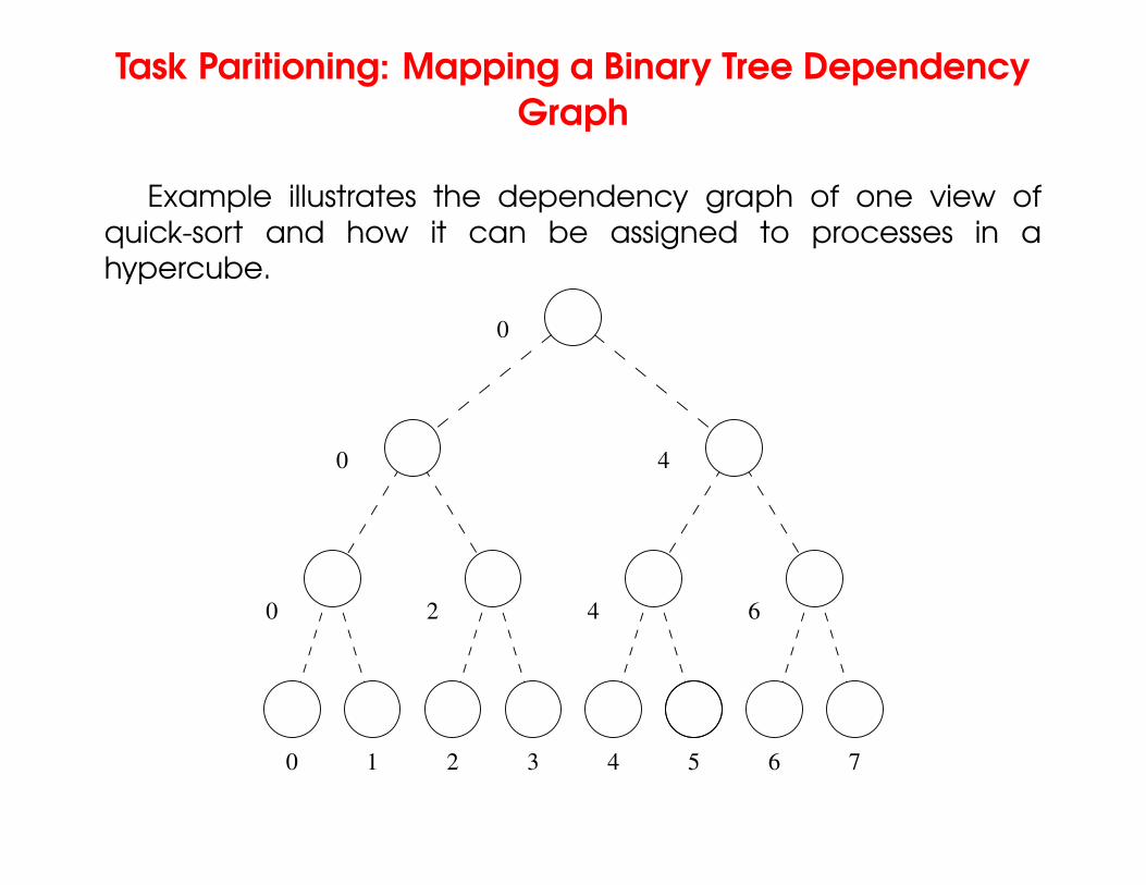
Task Paritioning: Mapping a Binary Tree DependencyGraph
Example illustrates the dependency graph of one view ofquick-sort and how it can be assigned to processes in ahypercube.
76
0
543210
0 4
0 2 4 6
– Typeset by FoilTEX – 75
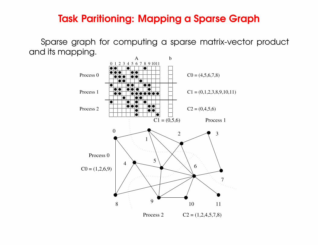
Task Paritioning: Mapping a Sparse Graph
Sparse graph for computing a sparse matrix-vector productand its mapping.
4 5 6 7 8 9 10110
C2 = (0,4,5,6)
21b
C1 = (0,1,2,3,8,9,10,11)
C0 = (4,5,6,7,8)
3
Process 0
Process 1
Process 2
A
C2 = (1,2,4,5,7,8)
2
4 6
13
5
11109
0
8
7
C1 = (0,5,6) Process 1
Process 0
Process 2
C0 = (1,2,6,9)
– Typeset by FoilTEX – 76
Hierarchical Mappings
• Sometimes a single mapping technique is inadequate.
• For example, the task mapping of the binary tree (quicksort)cannot use a large number of processors.
• For this reason, task mapping can be used at the top level anddata partitioning within each level.
– Typeset by FoilTEX – 77
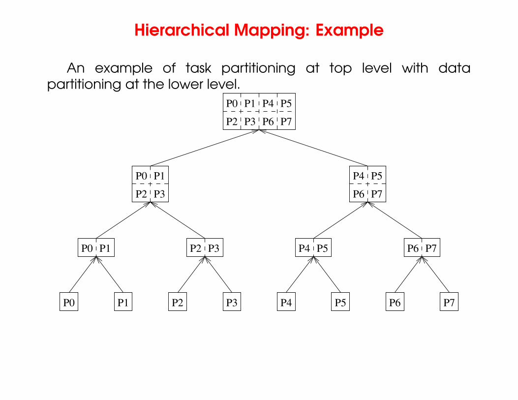
Hierarchical Mapping: Example
An example of task partitioning at top level with datapartitioning at the lower level.
P3
P0 P1
P2 P3
P0 P1
P3P2
P4 P5
P6 P7
P4 P5
P6 P7
P0 P1 P2 P3 P4 P5 P6 P7
P0 P1 P2 P4 P5 P6 P7
– Typeset by FoilTEX – 78
Schemes for Dynamic Mapping
• Dynamic mapping is sometimes also referred to as dynamicload balancing, since load balancing is the primary motivationfor dynamic mapping.
• Dynamic mapping schemes can be centralized or distributed.
– Typeset by FoilTEX – 79
Centralized Dynamic Mapping
• Processes are designated as masters or slaves.
• When a process runs out of work, it requests the master for morework.
• When the number of processes increases, the master maybecome the bottleneck.
• To alleviate this, a process may pick up a number of tasks (achunk) at one time. This is called Chunk scheduling.
• Selecting large chunk sizes may lead to significant loadimbalances as well.
• A number of schemes have been used to gradually decreasechunk size as the computation progresses.
– Typeset by FoilTEX – 80
Distributed Dynamic Mapping
• Each process can send or receive work from other processes.
• This alleviates the bottleneck in centralized schemes.
• There are four critical questions: how are sensing and receivingprocesses paired together, who initiates work transfer, howmuch work is transferred, and when is a transfer triggered?
• Answers to these questions are generally application specific.We will look at some of these techniques later in this class.
– Typeset by FoilTEX – 81
Minimizing Interaction Overheads
• Maximize data locality: Where possible, reuse intermediatedata. Restructure computation so that data can be reusedin smaller time windows.
• Minimize volume of data exchange: There is a cost associatedwith each word that is communicated. For this reason, we mustminimize the volume of data communicated.
• Minimize frequency of interactions: There is a startup costassociated with each interaction. Therefore, try to mergemultiple interactions to one, where possible.
• Minimize contention and hot-spots: Use decentralizedtechniques, replicate data where necessary.
– Typeset by FoilTEX – 82
Minimizing Interaction Overheads (continued)
• Overlapping computations with interactions: Use non-blockingcommunications, multithreading, and prefetching to hidelatencies.
• Replicating data or computations.
• Using group communications instead of point-to-point primitives.
• Overlap interactions with other interactions.
– Typeset by FoilTEX – 83
Parallel Algorithm Models
An algorithm model is a way of structuring a parallel algorithmby selecting a decomposition and mapping technique andapplying the appropriate strategy to minimize interactions.
• Data Parallel Model: Tasks are statically (or semi-statically)mapped to processes and each task performs similaroperations on different data.
• Task Graph Model: Starting from a task dependency graph,the interrelationships among the tasks are utilized to promotelocality or to reduce interaction costs.
– Typeset by FoilTEX – 84
Parallel Algorithm Models (continued)
• Master-Slave Model: One or more processes generate workand allocate it to worker processes. This allocation may bestatic or dynamic.
• Pipeline / Producer-Comsumer Model: A stream of data ispassed through a succession of processes, each of whichperform some task on it.
• Hybrid Models: A hybrid model may be composed eitherof multiple models applied hierarchically or multiple modelsapplied sequentially to different phases of a parallel algorithm.
– Typeset by FoilTEX – 85