Embed Size (px)
Citation preview

UNCLASSIFIED
AD NUMBER
AD464023
NEW LIMITATION CHANGE
TOApproved for public release, distributionunlimited
FROMDistribution authorized to U.S. Gov't.agencies and their contractors;Administrative/Operational Use; DEC 1964.Other requests shall be referred to Officeof Naval Research, One Liberty Center, 875North Randolph Street, Arlington, VA22203-1995.
AUTHORITY
onr ltr 9 nov 1977
THIS PAGE IS UNCLASSIFIED

UNCLASSRFWED
AD 4 64 02 3
DEFENSE DOCUMENTATION CENTERFOR
SCIENTIFIC AND TECHNICAL INFORMATION
CAMERON STATION ALEXANDRIA, VIRGINIA
UNCLASSEFIED

NOTICE: When government or other drawings, speci-fications or other data are used for any purposeother than in connection with a definitely relatedgovernment procurement operation, the U. S.Government thereby incurs no responsibility, nor anyobligation whatsoever; and the fact that the Govern-ment may have formulated, fuxrnished, or in any waysupplied the said drawings, specifications, or otherdata is not to be regarded by implication or other-wise as in any manner licensing the holder or anyother person or corporation, or conveying any rightsor permission to manufacture, use or sell anypatented invention that may in any way be relatedthereto.

SU-SEL-64-131
¢:stimating and Detecting the Outputs ofinear Dynamical Systems
by
C. S. Weaver miV , r -
C'-DJt OF D~
C-
<~-~ODecember 1964 _
-JUN '7 E$5 lii
Technical Report No. 6302-7Prepared under
COffice of Naval Research Contract
Nonr-225(24), NR 373 360
Jointly supported by the U.S. Army Signal Corps, the
CU.S. Air Force, and the U.S. Navy
(Office of Naval Research)
SYSTEMS THEORY LABORATORY
C O STnlFORD ELECTRONICS LABORATORIES5TMFORD UIllUERSITY •TAiFORD, [ALIFORnIA

DDC AVAILABILITY NOTICE
Qualified requesters may obtain copies of this report from DDC.Foreign announcement and dissemination of this report by DDCis limited.

SEL-64-131
ESTIMATING AND DETECTING
THE OUTPUTS OF LINEAR DYNAMICAL SYSTEMS
by
C. S. Weaver
December 1964
Reproduction in whole or in partis permitted for any purpose ofthe United States Government.
Technical Report No. 6302-7
Prepared under
Office of Naval Research Contract
Nonr-225(24), NR 373 360Jointly supported by the U.S. Army Signal Corps, the
U.S. Air Force, and the U.S. Navy
(Office of Naval Research)
Systems Theory Laboratory
Stanford Electronics Laboratories
Stanford University Stanford, California

q
ABSTRACT
This investigation considers three closely related problems: the
optimum filtering of stationary or near-stationary random processes with
unknown parameters from an infinite parameter set; estimation of the
state of a linear discrete dynamical system with nongaussian noisy inputs;
and applications of state estimation theory to detection. The form of
the optimum filter when t;he parameters are unknown is found to have
weights that are averages of simple functions of the signal and noise
spectra averaged over the parameter space. Practical methods for
implementation are given. The key problem in nonlinear state-variable
estimation is obtaining the joint density of the states and the observa-
tions in a convenient form. This problem is solved, and surface search-
ing is used to find the mode. The number of dimensions of the surface
is the same as the order of the dynamical system. A new approach to
linear state estimation is given; and this theory is applied to the
problem of detecting a gaussian signal in gaussian noise. A time-
invariant, near-optimum detector of small dimensions is derived.
- iii - ,SIL-64-131

CONTENTS
I. INTRODUCTION . . . . . . . . . . . . . . . . . . . . . . . . . 1
A. Outline of the Problem ......... .................. 1
B. Previous Work ...... ..... ...................... 2
C. Outline of New Results .......... ............ ... 3
II. STATEMENT OF THE PROBLEM AND MODEL OF THE PROCESS ... ...... 7
A. State-Variable and Sample-Value Representations of
Discrete Linear Systems ........ ................. 7
B. Model of the Process . .................. 10
III. OPTIMUM LINEAR SMOOTHING AND FILTERING .... ............ .. 12
A. Linear Filtering .......... ..................... 12
B. Optimum Linear Filtering and Smoothing ... .......... .. 14
C. Observations Through a Second Dynamical System ........ .. 18
D. Estimation with Partial Data ..... ............... .. 23
E. An Example of a Smoothing Estimation .. ......... .... 25
IV. APPLICATIONS TO DETECTION OF GAUSSIAN SIGNALS IN ADDITIVE
GAUSSIAN NOISE .......... ........................ ... 29
A. The Likelihood Detector ...... ................. ... 31
B. A Near-Optimum Detector Containing a Time-Invariant Filter 33
V. LINEAR FILTERING OF SIGNALS WITH CONTINUOUS UNKNOWN PARAMETERS 41
A. Magill's Solution for a Finite Number of Parameter Values 41
B. Filtering of Stationary or Near-Stationary Processes with
Parameters from an Infinite Set ..... ............. .. 42
VI. ESTIMATION WITH NONGAUSSIAN INPUTS ..... .............. .. 47
A. Introduction ..... ........................... .. 47
B. Propagation of First-Order Statistics .... ....... .. 47
C. Finding the Joint Density of the State Variable and theObservations ......... ......................... 52
D. Finding the Estimate ....... ................... ... 59
E. The Asymptotic Behavior of the Estimators as the Signal-
to-Noise Ratio is Increased ..... ............... .. 65
VII. CONCLUSION .......... ......................... .... 67
A. Summary .......... ......................... .. 67
B. Suggestions for Future Work ..... ............... .. 68
SEL-64-131 - iv -

APPENDIXES
A. Derivation of the Smoothing Equations. .......... 69
B. The Change in the Density of the Correlator Output . . .. 73
C. Derivation of the Form of the Near-Optimum Fiiter for
Continuous Parameter Processes .. .............. 77
D. Steady-State Error in a Wiener Filter. ........... 89
E. The Steady-State Minimum-Mean-Squared-Error Sampled-DataFilter .. .......................... 91
REFERENCES .. ............................. 94
v -SEL-64-131

ILLUSTRATIONS
1. An example of a discrete linear system ..... ............ 8
2. The dynamical system ......... .................... . 10
3. Flow diagram for smoothing ......... .................. 20
4. The model containing two dynamical systems ... .......... .. 22
5. The dynamical system for finding the error, E(k) ........ ... 22
6. The estimates of X(l) .............. ........ 28
7. The near-optimum detector ....... ................... ... 40
8. Block diagram of narrowband parallel filter system ....... . 78
9. Diagram for finding the error of the parallel filters ..... ... 81
10. The block diagrams for finding the error spectrum out of theith channel .......... ......................... ... 83
11. The convolution .......... ........................ ... 86
12. Synthesis of e- s T Hi and of the compact form of the adaptivefilter . ....... ............. .............. ... 87
13. A practical form of the adaptive filter ..... ......... . . 87
TABLE
1. Summary of the estimation equations ..... .............. .. 19
SEL-64-131 - vi -

SYMBOLS
a value of the i t weight of a tapped delay line
teith -*(i)a ij the j element ofA
.0.) the error in estimating xli
2ie steady-state mean-squared error of a Wiener filter
02 total mean-squared error of all the 0CT 0i
2 ero f-i)Leincrease in the mean-squared ero fB over the
minimu mean-squared error
f (t) characteristic function of u I(k)
m order of the matrix 0
qi (r) output of 01at the r th sampling tim
u,(k) the 2th component of U(k)
w,(k) the th component of W(k)
x2 (k) the 2t component of X(k)
a(k) a linear combination of the ua2(k)
A optimum linear estimator of x (k)
A k coefficient of Y(k) In filtering equation
A U()(X optimum linear estimator of x (I) given Y(j),...,Y(i)
vii -SIL-4-131

LA difference in impulse response between A and B
B system bandwidth
B1 output matrix for the two-system combination
Bk matrix multiplying X(k-1) in the filtering equation
giving X(k)
Ck matrix multiplying X(l) in the filtering equation
giving X(k) conditioned on X(i)
D' set of observed data
Ej matrix multiplying Y(i+j) in the equation giving
the near optimum estimate of X(i)
E(k) error in estimating X(k)
F(.) cumulative distribution function (cdf)
G transition matrix of the second dynamical system
G(Jiw) the ith narrowband filter
G0 (Jw) the optimum filter at the output of Gi(Jw)
lik matrix multiplying X(l) in the equation for the
gradient of the exponent of P[Y(l),...,Y(k)IX(l)]
H dynamical-system output matrix
J output matrix of the combination of two dynamical
systems
SL-64-131 - Viii -

J k that part of the equation for the gradient of the
exponent of P[Y(i),...,Y(k)IX(l)] that is not
multiplied by X(l)
K nonideal potentiometer setting
KU(k) covariance matrix of U(k)
Kw(k) covariance matrix of W(k)
K(k) covariance matrix of X(k) conditioned on all data
to Y(k)
KX(k) (i-m,i+m) covariance matrix of X(k) conditioned on
Y(i-m),...,Y(i+m)
Ky(k)(klk-I) covariance of Y(k) conditioned on all data 'to Y(k-l)
K covariance matrix of W
n
Ky Ycovariance matrix of Yn
L[Y(l),... ,Y(n)] likelihood ratio
N (f ) noise spectrum out of Gi(w )
N(k) noise input to the two-dynamical-system combination
N i noise power at the output of G (Jw)
P1.] probability density
R( ) autocorrelation function of x1 (k)
a() autocorrelation function of scalar W(k)
- ix - S-64-131

R x+w(iT) autocorrelation function of signal and noise
Si signal power at the output of G i(w)
S il(f) spectrum of signal and noise
S + see Eq. (D.1)ii
SiT see Eq. (D.l)
Snn(f) spectrum of noise
S (f i) signal spectrum at the output of Gi(iw)
Sss(f) spectrum of signal
S (Z) sampled-data signal spectrum
S X+W(z) sampled-data signal plus noise spectrum
T sampling period
U(k) noisy input vector to the dynamical system
W(k) dynamical-system output noise
W vector representing a sequence of scalar W(k),n
k = 1,2,...,n
X(k) dynamical-system state vector at the k th sampling
time
X(k) estimate of X(k)
SEL-64-131 - x-

Y(k) the observed random variable at the kth sampling
time
Y n vector representing a sequence of scalar Y(k),
k = 1,2,...,n
aparameter set
0tj element of 4
input matrix for the two-dynamical-system combination
71j element of P
w ia state of nature
r' the dynamical-system input matrix
r path of integration on unit circle
input matrix for the second dynamical system
see Eq. (6.17)
dynamical-system transition matrix
I(k) output noise generator of the two-dynamical-system
combination
- xi - SEL-64-131

ACKNOWLEnGMENT
Appreciation is expressed for the guidance of Dr. Gene F. Franklin,
under whom this research was conducted, and for the many helpful sugges-
tions of Dr. Norman M. Abramson. Special thanks are also due Dr. Rupert
G. Miller of the Stanford Statistics Department for several helpful
conversations-particularly concerning the proof of the first theorem
in Chapter VI.
SEL-64-131 - xii -

I. INTRODUCTION
A. OUTLINE OF THE PROBLEM
This investigation concerns the optimal estimation or detection of
a sampled, vector-valued stochastic process that may be generated by a
noisy discrete, linear, dynamical system. The system inputs are a
sequence of independent random variables, i.e., white noise. The system
output is corrupted with additive white noise. In the first part of
this report the white noise is assumed to be gaussian (linear estimation
is optimum); later, nongaussian inputs and output noise are assumed (in
general, nonlinear estimation will be optimum). The stochastic processes
may or may not be stationary and, for most of the report, the process
parameters will be assumed to be known a priori. In Chapter V, however,
consideration is given to the important problem of estimating the value
of the process when it is stationary or nearly stationary and when the
parameters are assumed to come from some infinite set with some a priori
distribution.
In this analysis, the word "estimation" will mean either filtering
or interpolation. An optimum estimate is defined as one that minimizes
a generalized mean-squared-error performance criterion or maximizes a
conditional density. Filtering is defined as the estimation of a present
value conditioned on all the past data. Frequently, the term "smoothing"
is used in place of interpolation or estimation of a past value condi-
tioned on all data to the present.
Engineering examples of the above processes are listed below. An
important example is a space vehicle in orbit. The equations of motion
when linearized correspond to a linear dynamical system. The atmospheric
drag may be represented as a noisy input. Range and velocity of the space
vehicle are measured over a noisy radio channel. This channel noise
constitutes the output noise. Usually, the noise, as it appears to the
velocity- and range-measuring equipment, is nongaussian.
An equally important example of this type of system is a rocket under
power. The noise inputs are caused by random variations in motor thrust
amplitude and direction. The trajectory information is also transmitted
over a noisy radio channel.
-1 - ,SEL-64-131

An example of a stationary process with unknown paraneters from an
infinite set is a satellite or space vehicle transmitting on an unknown
frequency due to uncertainty in the doppler shift or drift in transmitter
frequency. Determining and tracking this frequency are the central
problems in space communications. For most types of modulation, tech-
niques similar to those discussed in Chapter V provide by far the best
solution known. An example of a near-stationary process is a signal with
known parameters and unknown jamming, where the jamming corresponds to
an unknown output noise. Use of the moon as a passive reflector for
communications from one earth point to another is another example of a
near-stationary process. We might also include in this class a tracking
antenna system using conical scan. Here, the system gain is directly
proportional to the unknown signal strength which slowly varies.
B. PREVIOUS WORK
Kalman and Koepcke in their pioneering work [Ref. 1) have considered
the optimal filtering and prediction of sampled gauss-markov stochastic
processes when the parameters of the process are known. Rauch [Ref. 2]
has extended this analysis to include interpolation when the input noise
is gaussian, when there is no output noise, and when the parameters are
a sequence of independent random variables with known means and variances.
Widrow [Ref. 3] and Gabor et al [Ref. 4] have independently investigated
and constructed systems that adapt by using a noise-free sample of the
signal. Since in many practical situations the noise-free sample will
not be available, this type of adaption was not considered in this
investigation.
Magill [Ref. 5] has used the Hilbert space approach (approximately
concurrently with this investigation) to simplify the derivation of the
filter and interpolation of gausa-markov processes. He has also given
the form of the optimal estimate of a gauss-markov process when a finite
set of parameters is distributed in general according to some arbitrary
density. Cox [Ref. 61 discusses state-variable estimation of nonlinear
systems with gaussian inputs. His approach involves a system linearization.
SEL-64-.131 - 2 -

Work in this investigation contains an extension of Magill's adaptive
estimation for a finite number of parameters to estimation where the
parameters may come from an infinite set. The theory of nonadaptive
estimation is extended to include dynamical systems with nongaussian
inputs and output noise.
C. OUTLINE OF NEW RESULTS
This investigation gives solutions to three closely related problems:
1. The theory of adaptive estimation is extended to stationary ornear-stationary processes with parameters from some infinite
parameter set.
2. The theory of nonadaptive estimation is extended to includenonlinear filtering and interpolation of the state variables of adynamical system excited by nongaussian random inputs.
3. Methods are given for greatly simplifying the optimum detection
procedures when the signal can be considered as the output of alinear dynamical system excited by random noise.
Chapter II contains a description of the two main mathematical methods
of system description that are used in this report. This chapter also
contains a detailed description of the random process.
In Chapter III a new approach to the linear estimation of the state
variable of a discrete linear dynamical system is presented which shows
the close relationship between state-variable estimation and pattern
recognition. The estimation theory in Chapter III was inspired by, and
is a straightforward extension of, the pattern-learning theory developed
by Abramson and Braverman [Ref. 7]. In both cases, it is desired to
learn the conditional mean of a gaussian vector-valued random variable.
The equations for the mean and the covariance matrices derived by
Abramson and Braverman are almost identical to the filtering equations of
Chapter III. The author feels that the new approach is far simpler and
gives a greater intuitive insight than other methods that have been
suggested earlier.
The chapter also provides necessary background for the three chapters
that follow. A new problem is solved in Sec. C: estimation of state
variables when the estimates are taken through a second dynamical system
(as will very often be the case). Equations derived by Magill may be
- 3 - SEL-64-131

used to make these estimates; however, the order of Magill's matrix
equations can be twice as great as those presented here. If a large
amount of data is processed, the reduction in calculation could be
significant.
Chapter IV applies the theory of linear state-variable estimation
to the problem of detecting a gaussian signal immersed in additive
gaussian noise. It is shown that a long-standing conjecture about the
possibility of simplifying the detection procedure is often true. In
Kailath's solution (Ref. 8], the optimum detector contains an operator
that gives the best estimate of each signal sample value during the
detection interval based on all the data observed during the interval.
If several thousand data points are observed, a matrix of the same order
must be inverted. When the signal can be represented as, or 6pproximated
by, the output of a noisy dynamical system, the estimation equations of
Chapter III may be applied directly. The matrices to be inverted will
be no larger than the order of the dynamical system regardless of the
number of data points. Further simplification results if the estimator
of a sample value is truncated when the error covariance matrix shows
that there will be little reduction in mean-squared error by conditioning
on additional data points. A near-optimum time-invariant detector is then
shown to exist. The advantages of time-invariant circuitry when analog
networks are used cannot be overemphasized. Time-variable analog
networks of the complexity required in this problem are extremely
difficult and expensive to build. This form of detector is the form
most convenient to instrument, using the newly developing and powerful
methods of optical data processing.
Chapter V describes optimum estimation when the process is stationary
or near stationary and when the process parameters are unknown but may
assume any one of an infinite number of possible values. The term "near-
stationary" is used rather loosely. In practice, the filter will adapt
so quickly that good results may be obtained on processes many persons
would call highly nonstationary.
The estimator weights are functions of the parameters, and it is shown
that the optimum estimator is formed by taking the expected value of
the weights over the parameter space conditioned on the observed values.
SEL-64-131 - 4 -

It is then shown that the parameters enter into the weights as functions
of the signal and noise spectrum in a very simple manner. The optimiza-
tion procedure thus involves learning these spectral functions conditioned
on the data.
It is believed that this device will have numerous applications in
the field of space communications. As mentioned in Sec. A, a fundamental
problem is the frequency tracking of a narrowband signal. The usual
approach is to use frequency modulation or to insert an unmodulated
carrier. In either case a phase-locked loop may be locked onto the
carrier and used as a frequency reference for a narrowband filter.
Frequency modulation very often is not the best way to modulate, nor
does the inserted carrier contain information, and thus their use lowers
th system signal--to-noise ratio for a fixed transmitter power. In
electronic surveillance work, the opponent is hardly ever considerate
enough to include a tracking carrier! One of his favorite tactics is
to shift his transmitter frequency in a manner unknown to the receiver.
Such "carrierless" situations show the filter of Chapter V off to good
advantage since, unlike the phase-locked loop, it will automatically
center itself about the signal in the form of a narrowband filter.
Chapter VI discusses nonlinear estimation (including the best nonlinear
predictor) of state variables of linear systems with nongaussian inputs or
output noise. With the exception of the types cf distributions, the model
of the process is identical to that used for linear estimation. First,
there is a proof of the necessary and sufficient conditions for the dis-
tribution of the state variables to converge to the gaussian. The esti-
mates found in Chapter VI are either Bayesian or maximum likelihood, and
the key problem is finding the conditional density in a convenient form.
The Markov property of the state variables is used to simplify this
rather complex density and then surface-searching techniques are used to
find the mode. An important result is proof that near-optimum (linear or
nonlinear) estimates of the state of many dynamical systems do not
require conditioning on all available data, but may be made using only a
short sequence of observations. The length of this sequence may be related
directly to the rate of decay of initial conditions in the dynamical
- 5 - SL-64-131

system. The saving in computation time may be very significant. The
dimensions of the surface to be searched are the same as the order of
the dynamical system.
Use of this theory is envisioned in a situation such as the one
given below. Much of the ballistic missile work at Cape Kennedy is
concerned with measurement of missile accuracy. The trouble is that the
external ground-based measuring equipment is no more accurate than the
missile guidance and thus cannot offer any real check on the trajectory.
Any increase in guidance accuracy will completely swamp the measuring
equipment. (The seriousness of the problem has prompted the government
to issue a large contract for range modification, although it is the
opinion of many that the point of diminishing returns in measurement-
equipment accuracy has already been passed.) In data reduction the
standard procedure is to make a linear least-mean-squared estimate.
Since it is known that the statistics are nongaussian, nonlinear estima-
tion may offer a possibility of significant improvement. The asymptotic
behavior of the estimator as the output noise decreases is also discussed.
SEL-64-131 - 6 -

II. STATEMENT OF THE PROBLEM AND MODEL OF THE PROCESS
It is desired to form an estimate of a sampled-data, random-message
process corrupted by additive noise. The random message or the additive
noise or both may be nongaussian. The observable process (the process
from which the estimations are made) is assumed to be sampled, either
in scalar or vector form, and for most of this report is assumed to be
generated by processes with known statistics. In Chapter V, however,
it is assumed that the estimates are made of a process with unknown
parameters and that these parameters may come from an infinite set.
A. STATZ-VARIABLE AND SAMPLE-VALUE REPRESENTATIONS OF DISCRETELINEAR SYSTEMS
Two mathematical methods for describing linear discrete dynamical
systems are used in this report. The first is called the state-variable
representation, and the second is known as the sample-value representation.
Since many engineers are familiar with one or the other, but not with
both, the methods are discussed briefly in this section.
Consider the transfer function
0(z Zl-l - (2.1)O(1 = -1 V IYS(1 - aZ )(I - bZ 2
where u2 (Z) is a noisy control input and Y(Z) is the output. A block
diagram having this transfer function is shown in Fig. 1. The input
u1 (k) is a second input of noise alone. Let xl(k) be the value (or
state) of the output of the right-hand delay at the kth sampling
instant, and let x2 (k) be the value at the output of the other delay.
Then the state or state vector of the system is defined as
r x1(k)x(k) = (2.2)
[x(k)J
In general, any sampled-data transfer function may be reduced to block
diagram form with feedback around delays, and a state vector may be defined
with the values of the delay outputs at the sampling Instants as vector
elements.
- 7- SIL-64-131

Ui(k-1) :+
zY( k)
FIG. 1. AN EXAMPLE OF A DISCRETE LINEAR SYSTEM.
The vector X(k) may be found from a set of difference equations
that may be written as
X(k) = OX(k-1) + ru(k-i) (2.3a)
The matrix 4 is known as a "transition matrix" and is m x m where m
is the order of the system. This matrix may be time variable, but to
thsimplify notation, its argument will not be carried along. The ij t
element of 0, t is the gain between the output of the it h delay
and the input to the jth delay. The "input matrix" r is also m xm0 0and it determines where the input vector U(k-l) is applied to the
system.
The system output may be a vector or it may be scalar, and it usually
is a linear combination of the states. The output can be written as
Y(k) = iX(k) (2.3b)
where H is a q xm matrix (vector outputs), with q the number of
outputs. The H matrix also may be time variable. The system equations
for the system of Fig. 1 will then be
SIL-64-131 - 8-

X(k =. + jc (2.4a)0- b 2(k1l1u 2(k-lJ
Y(k) = (1 0] [1 (k) (2. 4b)
X2 (k/I
The second mathematical description will be used when the input and
the output of the dynamical system are both scalar. The output of a
linear system is a linear combination of the inputs, or
k
c(k) = Ia (ik) r(k-J) (2.5)
j=o
where r(k) is the input and c(k) is the output. The system may be
thought of as a tapped delay line similar to the one shown in Fig. 12
of Appendix C. If r(t) is a bandlimited continuous function with
value r(k) at the kth sampling instant, and if the time between
samples, T, is less than 1/2B, where B is the bandwidth, the well-
known sampling theorem [Ref. 9] shows that there is a one-to-one cor-
respondence between the sequence r(k), k = 0,1,...,k , and r(t) over
the interval [0, k T]. There is also a one-to-one correspondence
between the sequence of c(k) and c(t) over the same interval. For
a time-invariant system, the a (k) are the coefficients in the series
expansion of the system Z-transform.
If the r(k), k = 0,1,...,k are the (ko+l) elements of a vector
called the "input vector," and if the c(k), k = 0,1,...,k o, are the
(ko+l) elements of the "output vector," the two vectors are related by
the following matrix equation. (The square matrix will be called the
"transfer matrix.")"C(O) 'ao0(0) r(O)
c(1) a1(l) So () r(l)
= a2 (2) al(2) a(2) (2.6)
- 9 - SNL-64-131

B. MODEL OF THE PROCESS
The message process will be generated by random inputs, U(k), to
the system shown in Fig. 2. It is assumed that U(k) is independent of
U(j) for j # k. The element u (k) is also assumed to be independent
of ui(k) for i i.
FIG. 2. THE DYNAMICAL SYSTEM.
Much use will be made in this report of a characteristic of X(k)
called the (strict) "Markov property." This property is defined by the
relationship
F[X(k)IX(l),... ,X(k-l)] = F[X(k)IX(k-l)] (2.8)
where F(') is the cumulative distribution function (cdf). In other
words, the density of X(k) given all the X(J) up to X(k-1) is the
same as the density conditioned only on X(k-1). From Eq. (2.3a) it is
seen that if X(k-1) is given, then the only random variable on the
right is U(k-1). Since U(k-1) is independent of U(J) for j -. k,
the density of X(k) is entirely determined by X(k-1) and U(k-1).
If U(J) is a gaussian random variable, the process is known as a
"gauss-markov" process.
The message process is assumed to be transferred over a physical
channel (such as a telemetering link) and noise will be added. In our
model, this noise is indicated by the vector W(k), and Eq. (2.3b) will
be modified to
Y(k) = HX(k) + W(k) (2.3c)
SEL-64-131 - 10 -

Estimations of X(j) will be made by observing (the observable process)
the sequence Y(1),... ,Y(k).
Both U(k) and W(k) are assumed (without loss of generality) to
have zero mean. The vectors U(k) and W(J) will be independent for
all j and k, and W(k) will be independent of W(j) for j k.
Two types of covariance matrices are used frequently in this study.
The first is called a "state-variable covariance matrix" and is denoted
by the letter K. For example,
E[X(k) X(k) t ] = KX(k) (2.9a)
E[Y(k) Y(k)t = KY(k) (2.9b)
ErW(k) W(k)t) = KW(k) (2.9c)
where superscript t means the transpose.
The second type of covariance matrix is called the "time-series
covariance matrix." An example would be
Ks E :1 (2.10)
L(k),
- 11 - . SEL-64-131

III. OPTIMUM LINEAR SMOOTHING AND FILTERING
This chapter discusses linear smoothing and filtering. The
estimators will be derived by assuming that the input random process
and the output noise are gaussian. So, the first section will contain
a brief discussion of linear filtering of nongaussian processes with
either gaussian or nongaussian output noise. Section A also contains
a comparison of the Bayesian and the maximum likelihood estimation of
state variables. Section B contains the derivations of the filtering
and smoothing routines. In many practical applications, the observations
will be made through a second dynamical system, and Section C contains
a derivation of the required modifications of estimating procedures.
A. LINEAR FILTERING
The two classes of estimators to be considered in this report are
Bayes estimators and maximum likelihood estimators.
Definition: A Bayes estimator X(Ji) is one that minimizes the
expected risk,
p(i) = f [Li()j,x(j)1 P(x(j)jY(l),...,Y(k)] dX(J)
where LtX(J),X(j)] is the loss and X(J) is the estimate of X(J)
given Y(l),...,Y(k).
If
L[X= 2 (3.1a)itXC),X(J)] ij
it can easily be shown that
i(j) = E(X(j)IY(l),...,Y(k)) (3.1b)
The loss function for the Bayes estimate will always be that defined in
Eq. (3.1a), i.e., minimizing the mean-squared error.
SEL-64-131 - 12 -

Definition: The maximum likelihood estimate of X(J) is the X(J)
that maximizes P[X(j),Y(l),...,Y(k)].
It is frequently convenient to find this maximum by setting the
gradient of injP[X(J)jY(l),... ,Y(k)]) with respect to X(J) equal to
zero. The elements of the gradient vector are known as "likelihood
functions."
If P[X(J)IY(l),...,Y(k)] is symmetric about the highest mods, the
conditional mean and the maximum likelihood estimate coincide. Such
conditions exist if X(J) and W(j) are gaussian.
In Sec. B, the Bayes estimators for gaussian inputs are seen to be
linear. Now, if the actual states are taken from the dynamical system
and subtracted from the corresponding estimator output to obtain the
error, the system from the noise inputs to the error outputs is still
linear. Then, the error covariance matrix will be Just a linear trans-
form of the input covariance matrix plus a linear transform of the output
noise covariance matrix. The mean-squared error is the tace of the
error covariance matrix. In other words, the mean-squared error of the
filter that is optimum for gaussian input and output noise is a function
only of the input and output noise covariance matrices. If a filter is
designed to be optimum for a gaussian input process with a given covariance
matrix, the mean-squared error of this filter, when the input is non-
gaussian with an identical covariance matrix, will be the same as the
gaussian input mean-squared error.
In Chapter IV (for example) it is seen that if one asks the question,
What is the linear circuit that will give the minimum mean-squared error?
the answer is found to be a function Of the input variance and covariance
only. Then, the filters derived in this chapter are the best linear ones
for all densities with the same covariance matrix. If any improvement
is to be gained for nongaussian processes, it necessarily will be a
nonlinear operation. Nonlinear smoothing and filtering are discussed
in Secs. B and C, Chapter VI.
- 13 - SEL-64-131

B. OPTIMUM LINEAR FILTERING AND SMOOTHING
In this section, the optimum filter is first derived. Next, the
optimum smoothing routine is found and it will be seen that it contains
filtering as a subroutine. The model is shown in Fig. 2 with W(k) and
U(k) gaussian. The filtering problem then is to estimate X(k) given
all values of Y up to Y(k). As noted in the last section, the
optimum estimate is the conditional mean of the quantity to be estimated.
In other words, if it is desired to estimate X(k), write the density
P[X(k)IY(k),Y(k-1),...,Y(l)], and find its mean. Later, it will be
shown that this mean is identical to the mean of P[X(k)IY(k),R(k-1)],
where X(k-l) is the estimate of X(k-1) given Y(l),... ,Y(k-l). So
our problem is reduced to finding this second mean.
Using Bayes' theorem, write
P[X(k)IY(k),X(k-1)] = P[Y(k)jX(k),i(k-l)] P[X(k)IX(k-1)] P[i(k-l)l (3.2)
1'[X(k-l) ,Y(k)]
Since this density is gaussian, the mean will be the value of X(k) that
minimizes the exponent of the density.
Note that X(k) is contained only in PIIY(k)?X(k),X(k-l)] and
P[X(k)iX(k-)]. Referring to Fig. 2, it is seen that
P[Y(k)IX(k),i(k-1)] = P[Y(k)IX(k)] = N[HX(k),Kw(k) ] (3.3)
where K W(k is the covariance matrix of W(k); [N(A,B) denotes a
normal density with a mean vector A and covariance matrix B]. The
vector X(k-1) is the mean value of X(k-1) given Y(k-l),...,Y(l).
Then the mean value of X(k) given X(k-l) *is X(k-1). Let the
covariance matrix of X(k-1) about X(k-1) given all data up to Y(k-1)
be K^ (The subscripts on the covariance matrices denote theX(k-l)'
random variable.) The covariance matrix of tX(k-l) about X(k-l) is
K^ 4t ("t is the transpose of ) Since X(k-1 is independentx(k-l)of U(k, we have
t t'P[X(k'1X(k-1'' Nr.X(k-1 , _ + , k -l ( .
SEL-64-131 - 14 -

Assume that K W~)is not singular. Thus, the product can be written as
2w]tk)k
P(Y~k X~k]Pf ~k)Ii~k-)3 = (cost eXpE .)]tt(k) HX(k)]tKO ) (k )-H k
(3.5)where
K A Oi 0t +rPt (3.6)X(k) = x(k-1) U(k-l)
The exponent will be minimized when the gradient of the quadratic in
Eq. (3.5) is zero.
If Q is any syimmetric matrix, Tj is a vector, and if
= (HX- TI) tQ(HX- TI)
then the gradient of 4t with respect to X is
grad 0 = 2H Q(HX - TO (3.7)
Also, the gradient of a sun of quadratics is the vector sum of the
gradients of each quadratic. If the mode of Eq. (3.5) in found by
setting the gradient with respect to X(k) of the exponent equal to
zero, and solving for X(k), the optimum estimate of X(k) is:
X(k) H [li K )H + H~)] [11 KkY(k) + K- O)X(k-l)] (3.6)
The covariance matrix K^ Is found from Eq. (3.5) by taking theX(k)inverse of the sum of the terms that are premultiplied by X and
postmultiplied by X or
Kick) = lt Vk~ + xk)]
Note that K^ is not a function of Y.X(k)-15 - SZL-64-131

If the estimation procedure is stated at k = 1, KX(l) must be
known. Assume that the dynamical system is turned on at k =-M and
the initial conditions are zero at that time.
M +1
x(l) 1 0 M 0-i+l Pt(i-M 0-1) (3.10)
i _=0
Then,
M +10 M -i+l *M-i+l t (3.11)
1KX(l) 1 0 rKU(_M _) rt ( 0
i _=0
The one remaining quantity to be specified is X(i).
P(Xl~l(1) =pryf1) I x(Ij1pIx(l )1(.2
P[Y(l)IX(l)j PEX(l)] = (const) exp[.!I[Y(l) - HX(l)jt Kw11)(Y(l) - IX(l)]
+ tx(l) - i( 1 ))t KW(l)X(l) - i(l)l} (313
where i(l) is the a priori mean of X(l) f(i) is zero if the
initial conditions in Eq. (3.10) are zero]. Setting the gradient equal
to zero gives
=J [Ht Kw lH + K' ~ WjtK ( KxX(lI~ l XWj I() 1 +(.4
The matrix K-(1 is obtained from Eq. (3.9).
SEL-64- 131 - 16-

Equations (3.6), (3.8), (3.9), (3.11), and (3.14) completely specify
X~k) given i-(k--l) and Y(k). If it is desired to estimate X(k) given
Y(k),...,Y(l), write
P[X(k)IY(k),.. .,Y(l)] =P[Y(k)IX(k),Y(k-l),... ,Y(l))
P[X(k)jY(k-l),...,l)
P[Y~-l),..,Yl)](3.15)
The function OX(k-l) is the mean of x(k) given that Y(k-l),...,Y(l)
have occurred. Notice that K X~)is not a function of Y(k-l),...,Y(l);
therefore,
P(Xk~j~k-),..,YI)]= PCX(k)lX*i(k-l)]
Again, it io obvious that
P(Y(k)tX(k),Y(k-l),...,Y(l)) wNliX(k)IK W(k)] (3.16)
so that Eqs. (3.6), (3.8), (3.9), (3.11), and (3.12) also specify 1(k)
given Y(k),...,Y(l).
In the smoothing problem, it is desired to estimate the value of
X(I) given Y(k),...,Y(l). Following a similar method, the conditional
density is considered. To obtain the estimate in recursive form, It is
desired to express the gradient of in P(X(l)jY(l),...,Y(k)] with respect
to x(l) as a function of the gradient of In P[X(1)IY(l),...,Y(k-l)].*
=P[X(l)] P[Y(l)IX(l)] P[Y(2)IX(l),Y(1)1,... IP(Y~klI)IX(l),Y(l)I...,Y(k-2)1
(3.17)
Throughout the balance of this report all gradients will be taken withrespect to X.
-17 - 81L-64-131

Since on the right side of Eq. (3.17) X(1) is contained only in the
numerator,
grad [ n P[X(1)IY(l),... ,Y(k-l)]j'a grad J n P[X(l),Y(l),...,Y(k-I)]}
(3.18)
Similarly,
grad lin P[X(l)IY(l),...,Y(k)]j o grad [en PtX(l),Y(l),...,Y(k)1I
- grad [en P[X(1)IY(1),...,Y(k-l)]
+ grad 1ja P[Y(k)jX(l),Y(l),...,Y(k-l)]j
(3.19)
So the gradient conditioned on data to time k is obtained by a simple
addition of
grad [en P[Y(k)IX(l),Y(l),...,Y(k-1)]
to
grad [en P[X(1)!Y(l),...,Y(k-l)]j
Setting this new gradient equal to zero and solving for X(l) giv-s the
value of X(l) that maximizes P[X(1)IY(l),...,Y(k)].
The smoothing equations are given in Table 1. Because of the large
amount of algebraic manipulation required, the details of the derivation
are reserved for Appendix A. The flow diagram for smoothing is shown
in Fig. 3.
C. OBSERVATIONS THROUGH A SECOND DYNAMICAL SYSTEM
Very often the observations will be made through a second dynamical
system. For example, if state-variable estimation is used to estimate
orbital parameters of a space vehicle, the output of the radio link will
be fed to an analog-to-digital converter. These converters have a
limited dynamical (amplitude) range, and a narrowband filter usually must
be placed after the broadband i-f amplifier to reduce the noise variations.
The filter bandwidth may be small enough to influence the statistics of
Y(k) (i.e., the noise may no longer be "white" and the covariance matrix
of HX(k) will be changed).
SEL-64-131 - 18 -

TABLE 1. SUMMARY OF THE ESTIMATION EQUATIONS
Filtering Eq.
X"(k) = [H tK- I)H + I ]k)1 [HtKW-kY(k) + K- 1 Ok(k-l) (3.8)
K1k HtWtk) HK-X~k)] (3.9)~k
[H t 4K-. 1 ~ H pt (3.6)Kx(k) x (k) (k]-l
u01M -i+1 u-
K =) 0 r%(,_, 0 _,)r (3.11)
=~l [HtK 1 )ui+K )]luK )Y ) + K-Xl)i(i )] (3.14).
Smoothing X(i)
~( k- =[~~~KY(k)(kklzk_ 1 k-l1]
[Ctl'btutK(k) (kIk-l+(k) - H0A(k-l) JX()+ Jkl] (A.8)
k- 1 IIHtKW'i)H + K.X'(1)-f (A .5)1=2 I(i=2
K- [1 utc(klk-l)isCk + ~k](A.11)
in t_4tHtC I (kjk1l)jY(k) - H~s-(kl)IX(l)4+ Jkl (A.12)
aK1 + HtK.W'1 )H + OtHtK() +HrK r)t Ht I HO (A.9)
K Y(k) (k 1k-i) HIi (kl1) 0 + rxuK U-) r t]Ht + 1W(k) (A. .6)
With No Earlier Data
j 0 mt~iWz 8 HK )rtlt] - .Y(2) + HtKw'Y(iL) + K- 1I(1 (A.10)2 t (2+'U2With Earlier Data -X
w 0 t t t[%2 Hr( )rtit1-l Y(2) + HtK4w,) + C .(o)2 LW) u2) Jx)
where X(O) is the estimate of X(0) given all the data to k =0.
-19 - 53-64- 131

H'w.gN 9K D~lt
C11-1
FIG. 3. FLOW DIAGRAM FOR SMOOTHING.
In this section, methods for finding the optimum estimates of X(k)
of a function of the second dynamical system will be given. The two
dynamical systems will be combined and a single set of system equations
will be written. Noise will be added to the output of the second system,
and it will be shown that, as the variance of this noise is reduced to
zero, the variance of X(k) approaches the minimum mean-squared error
of 9(k) in a known manner. Then, some small output noise may be
assumed and an estimator may be designed using the combined system
equations and the estimation equations of the last section. This esti-
mator may have a mean-squared error as close to the minimum as desired.
Consider the two dynamical systems shown in Fig. 4. The matrix A
is an input matrix, VG is a transition matrix, and J is an output
matrix (or vector). Define the following quantities:
X(k)M(k) =(3.20)
r.x(k)J
SEL-64-131 - 20 -

(3.*21)
7 = [2L (3.22)
0
.(k(k)N(k) - (3.23)
Lu(k)J
Lo '01lB1= I IJ (3.24)
Then, the system equations for the double dynamical system are
M(k) = Oh(k-l) + 7N(k-l) (3.25)
Y(k) = B'M(k) + C(k) (3.26)
The vector n(k) is independent of $(j) for k 4 J, and the
elements of a(k) are assumed gaussian. The elements of K A(k) ,
a diagonal matrix, are assumed to have a known, very small, upper bound.
This small noise generator, of course, is always present in physical
situations but Its parameters are usually unknown. If, for design pur-
poses, we choose a K (k) arbitrarily-whose elements are the bounds,
we are assured by the following argument that the mean-squared error in
estimating M(k) from Y is not greater than that error calculated
assuming the noise covariance was at the bound. Thus, a bound on per-
fornce can be found from the bound on noise power.
The block diagram for the error
1(k) = [M(k) - {Ck)] (3.27)
Is shown in Fig. 5. Let M(k) be the output of the best linear estimator
for K.(k) equal to its upper bound. The error covariance matrix is a
sum of a linear (matrix) transfor-aation on K (k) and a linear
- 21 % BEL-64-131

Wa~k)
FIG. 4. THE MODEL CONTAINING TWO DYNAMICAL SYSTEMS.D is a unit delay.
MULTIDIMENSIONALPOTENTIOMETER
y 0 9 INWIklkN~k) _. +v fl '
FIG. 5. THE DYNAMICAL SYSTEM FOR FINDING THE ERROR, E(k).
transformation on KN(k-). The mean-squared error is the trace of this
transformation which is the sum of the trace of the transformation on
K R(k and the trace of the transformation on K N(kI. Reduction in
the elements of K R(k) will decrease the mean-squared error since each
diagonal element of the transformation on Kn(k) is greater than or
equal to zero. Then, the designer knows that he can lower the upper
bound until the mean-squared error is within specifications.
If the physical situation assures him that the bound is higher than
is actually the case, the estimation equations of Sec. B may be used
directly by substitution of N(k), 7, 0, B', efT(k), and M(k) for
U(k', T, F, H, W(k), and X(k), respectively.
SEL-64-131 - 22 -

D. ESTIMATION WITH PARTIAL DATA
In this section is given the form of the optimum linear estimate
when some of the data are missing. Many practical situations arise in
which a complete set of observations is not available. An example
would be estimation of a rocket trajectory where telemetry was temporarily
lost. Another example would be when telemetry is lost during a midcourse
maneuver. Frequently the system output is telemetered on a time-shared
basis, so that the data are available only periodically.
Assume that all the data are available up to time k and are lost
at time (k+l). Then X'(k) may be calculated using Eq. (3.8). Note that
x(k+i) - 01 x(k) + 0Z' r u(j+r) (3.28)
r=O
Taking the expected values conditioned on Y(l),...,Y(k) (since the
U(J+r) have zero mean and are independent of Y(l),. ..,Y'%k)] gives
i"(k+i) - 0iX(k) (3.29)
The covariance of X(k+i), Kf(kli)(k+ilk), conditioned on Yl,.,~)
is
i- 1
K^ (k+ilk) - )ix (it + 7 r(,rt (3.30)X(k+i)' Ix0k)U(j+r)(rtr-O
Assume that the data are regained at time (k+j). Then the best
estimate of X(k+i) in the interval from (k+l) to (k+j-l) is given
by Eq. (3.29).
Since new data are available at time (k+j), write
P(X(k+j)IY(k+j),Y(k),.. .0()
=P[Y(k+J)IX(k+.1)]PfXik+j~iY~k : : : :: IPrY(k),...Y(l)] (3.31)
and
P(X(k+J)IY(k),...,Y(l)] N(4Oj2(k); Ki(k+j ) (k+jlk)] (3.32)
-23 - SEL-64-131

Then the optimum estimate of X(k+j) is
^~ k j) IH FI H - +(k+jlk)(3h1 = (k+ + x(k+J) ('j
3.3 )+ j
The covariance of X(k+J) conditioned on the new data is now
-Ktl (3.34),(k+j) = [HK(k+J H (k+j) K' L~~j) +K'(~ )(kJ k)j (.34
The estimation is continued using Eqs. (3.6), (3.8), and (3.9) until a
new loss in data occurs. Then Eqs. (3.30), (3.33), and (3.34) are used
again.
If smoothing is to be performed, Eq. (A.13) will, of course, not
contain the missing data; i.e.,
P(X(kiJ)IX(l),Y(2),...,Y(k)) - N[HOJR(k);Ilcj(k^ j)(k+Jlk)Ht + J(kJ)]
(3.35)
The new gradient added by Y(k±j) is
-2t(O Ht t[Kfl(k~jlk)Ht+Kk ) (Y(k+j) - HJ~)
Then
X(I) :(OJ)tt[H I( (k+jlk)Ht + w(k+J HO Ck + k)
.tc(,t)tH u~(~)(k+jtk)Ht +'wkaj (Y(k) - HA~(k)] + Jk(3.36)
When the next observation, Y(k+j+l) arrives, Eq. (A.8) is used. It
should be noted that
Ck+j 2 0Jc k (3.37)
and that
Ck+j+l V [ntK; + -kJl) -k+j+l) Ck(
SEL-64-131 - 24 -

E. AN EXAMPLE OF A SM007HING ESTIMATION
A simple (but typical) dynamical system will be assumed. The
matrices will all be scalar.
0 = 1, H =l1, r 1
The covariances will be
K =1, 1U~k) KW(k) - 4
It is desired to estimate X(l) based on the observations Y(l)-, Y(2),
and Y(3).
The random numbers u(k) and W(k) were obtained from a gaussian
random number table with the variance adjusted to 1 and 1/4 respectively.
The numbers chosen were:
k UkW(k)
1 0.77 0.41
2 -0.33 -0.11
3 -- -0.06
From Eq. (2.3a),
X(k) = 1 X(k-l) + u(k-l)
Y(k) = X(Ic) + W(k)
Then X(k) and Y(k) are:
k 3LJ Y(k)
1 1 1.41
2 1.27 1.61
3 0.31 0.25
- 25 S 5-64-131
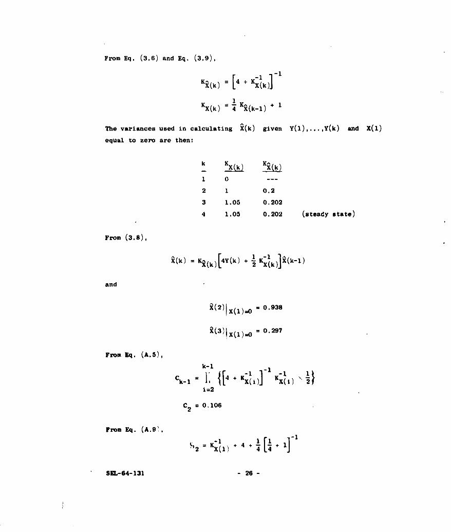
From Eq. (3.6) and Eq. (3.9),
IX(k) i KX(kJ
K -1
x(k) - 4 ^ (k- 1 ) + 1
The variances used in calculating X(k) given Y(1),...,Y(k) and X(i)
equal to zero are then:
k Kxk _________ x (k)
1 0 ---
2 1 0.2
3 1.05 0.202
4 1.05 0.202 (steady state)
From (3.8),
X(k) = K- k)[4Y(k) + "K-1 (k-1)
and
R(2)IX()l 0= -- 0.938
X(3)jX(l)-O = 0.297
From Eq. (A.5),
k-1 -
Ck k- j [4 + K-~) Kx-i 1
i=2
C 2 = 0.106
From Eq. (A.91,
S= +4*KX-- + 4 +21-x-1) 4 14
SEL-64-131 - 26 -

The matrix K 1 in Eq. (A.10) is the covariance matrix of X(i)
given that U(k) has been applied long enough for the dynamical system
to reach steady state at k = 1. From Eq. (2.3a),
00
x(1) = I OiU(-i)
i=O
Then the steady-s.tate variance of X(l) is
x(l) 2 l=
i=O
and
2 5.53
From Eq. (A.lO)
]~-'2 =II + I Y(2) + 4 x Yl)
= 6.12
where X(l) = 0. Then
X[(ly(l),Y(2)] = 6 = 1.11
From Eq. (A.6)
KY(3 ) (312) = 1.30
From Eq. (A.i),
5.5323
From Eq. (A.12), J 3 6.11. Then
X[iIY(l),Y(2),Y(3)] 1.10
Equation (3.14) may be used to find X[IIY()3 = 1.16.
- 27 - SEL-64-131

The results are summarized in Fig. 6. The estimator reaches steady
state after only two observations. Further examination will show that
the weights of all Y(k) after Y(2) are very nearly zero. Such very
short estimator impulse responses occur in a large number of practical
problems with typical dynamical systems. As will be shown in Sec. D of
Chapter VI, the estimator may always be truncated after a small number
of terms except in the rare case of a dynamical system with an extremely
high Q. Usually, short impulse estimators for even these cases may be
found by choosing an equivalent model of the dynamical system with a
much lower sampling rate.
x(O)
1.220 h11 1.101,0-------o _ 0_
TRUE VALUE OF X(1)
I 2 3NUMBER OF OBSERVATIONS
FIG. 6. THE ESTIMATES OF X(l).
SEL-64-131 - 28 -

IV. APPLICATIONS TO DETECTION OF GAUSSIAN SIGNALSIN ADDITIVE GAUSSIAN NOISE
In this chapter the theory of linear state-variable estimation is
applied to the problem of detecting a gaussian signal immersed in additive
gaussian noise. The optimum detector contains an operator that gives
the best estimate of each signal sample value during the detection
interval based on all the data observed during the interval. Typically,
several thousand data points may be observed. In the usual derivation
of the optimum detector (see Sec. A), a matrix of an order equal to the
number of data points must be inverted. When the signal can be repre-
sented as, or approximated by, the output of a noisy dynamical system,
the estimation equations of Chapter III may be apr'ied directly. The
matrices to be inverted will be no larger than the order of the signal-
generating dynamical system, regardless of the number of data points.
Further simplification results if tho impulso responsc of the
est.mator of a sample value is truncated when the error covariance matrix
shows that there will be little reduction in mean-squared error by
conditioning on additional data points. A near-optimum time-invariant
detector is then shown to exist.
The chapter begins with a definition of the likelihood ratio. Then
follows a derivation of the optimum detector that requires an inversion
of a matrix of high order. The final section derives the near-opti
time-invariant detector.
Let the observations Y(k) be
Y(k) - xI(k) + W(k) (4.1)
when the signal xI(k) is present (hypothesis w 1 is true), where W(k)
is additive gaussian noise. When no signal is present (hypothesis W2
is true),
Y(k) - W(k) (4.2)
The quantities Y(k), x (k), and W(k) are assumed to be scalar.
- 29- 8=,-64-131

When -a statistical decision is made between the presence of a signal
in noise, or noise alone, the best decision is based on the likelihood-
ratio test (Ref. 10, p. 3183. This ratio is defined as
L(Y(l), . .. ,~) [~),,Y(n) ~ 2 (4.3)
if
we say a signal is present, and if
L[Y(l),...,Y(n)) < 13(4.4b)
we say there is noise alone.
Assume the signal is gaussian with "zero mean" covariance matrix
Kx = E IxX t In
where
x l(l)
X X 1 (2)
x I(n)
Assume that the noise has zero mean and denote the covariance of the
signal-plus-noise vector by KY Thenn
K~ K% +K X (4.5)a n n
P[Y(l),. .. ,Y(n)jw1 3 - (const) exp{ I~ Yt KY IY} (4.6)
and
(coat) x4 .1 Y1t ,~l Y.) (4.7)
83-64-131 -30 -

Since the logarithm is a single-valued function, one might just as well
consider
Ln Y(),...,Y(n)" (const) -Y KY-1 Y - Yt 41 Yn (4.8)n n
Or, a signal is said to be present if
YKY Yn + Yt n lr Yn >70 (4.9)n n
It is noticed that the dimension of Y equals the number of data pointsn
used in the decision. The inversion of Kyn may be difficult or impossible
in problems involving a great deal of data.
A. TIit LIKELIHOOD DETECTOR
This section describes how to calculate the left side of inequality
(4.9). It will be shown shortly that this calculation requires finding
optimum estimates of the signal conditioned on the observed data. First,
the optimum smoother will be derived in a form different from that
derived in Chapter 11I.
A linear estimate of xI(i) given Yn will have the form
n
I aij Y(J) (4.10)
Jul
The error is
n
e(i) = XI() -I aj Y(J) (4.11)Jul
and the man-squared error is
S2 (i) - R x(0) - 2 1 a 1jRx(iJ) + a aji~aklRX (J-k) (4.12)
Jul kal Jul
The following treatment is due to T. Kailath (Ref. 6].
- 31 - S-64-131

where
Rx(i-j) - E(x (i)x1(j)] (4.13)
and
R ,+W(J-k) - E i .j1) + w(J)1x 1 (k) + W(k)) ~ (4.14)
To minimize e 2(i), take the partial derivativen
() n 02R (i-J) + 2 a kR +w(J-k) J - 1,2,...,n (4.15)~kul
Thus there are n simultaneous equations giving a solution for the
n a t. If this process is repeated for each i, the result may be
written as a matrix equation
(a i] K.%
which has the solution
A - ,, (4.16)Un
thThe dot product of the i row of A with Yn will give the minimum
mean-squared-error linear estimate of xI(I), given Y n or
1 .- (4.17)An "n
I I (n)J
Notice that
A (K% (4.18)
n n
n n
SIL-64- 131 - 32 -

Then
Ky1 K _ K; A (4.19)n n n
Substituting Eq. (4.19) into Eq. (4.9), we can now say that a signal is
present if
yt Kl AY > 7 (4.20a)n n 0n
or
ytK W Xn > 70 (4.20b)n
As the length of the sample of signal and noise or the sire of n
grows, so does the dimersion. In practice, it is impossible to invert
matrices of dimension greater than four or five hundred. In a typical
planetary radar detection problem, the signal sample may be 30 &in long
with a bandwidth of 5 cps. Then, the dimension of Kn will be4 Yn
1.8 x 10 . If such problems are to be solved optimally, a more efficient
design procedure must be found.
B. A NEAR-OPTIMWK DETBCT0R CONTAINING A TIME-INVARIANT FILTER
The remainder of this chapter will show that, for Y(k) stationary
and n sufficiently large, there exists another matrix representing a
time-invariant filter whose mean-squared error averaged over i is
arbitrarily close to the mean-squared error of A averaged over I.
Furthermore, the norm of the difference between the i t h row of thisthnew matrix and the I row of A tends toward zero as i increases.
As shown in Appendix B, this implies that, as m increases, the detec-
tion error probabilities using the time-invariant filter are arbitrarily
close to those of the detector employing the filter represented by A.
The linear smoothing equations of Chapter III may be used to find
the time-invariant filter. It will be shown that only a small sequence
of the elements of Y are required at one time, so that computernstorage requirements may be considerably reduced.
- 33 - SZL-64-131

Assume that a filter with impulse response is represented by the
vector A(I) Let this filter give the optimum 6stimate of xI(i); i.e.,
A Y n (4.21)
Let another filter with impulse response vector B(i) give another
estimate of x (i). We now prove that a bound on the vector difference
between A(i) and B may be computed from the difference in mean-_+(i ) -(i)
squared errors of A and B
Theorem: If [A(i) It Yn is the minimum mean-squared error estimate
of xI(i), given Yno and [-(i)It Yn is some other linear estimate
of xl(i) with an increase in mean-squared error of e 2 ovef that
of t (i)A t Yn' then
(4.22)2
S0 w(i)
where E WnW - w(i), and Ai) is defined as
(i) ().()
Proof: Let Aaij be the Jth element of Ai)
n n
2 (ai + As j)(ai +'A Ik)R a (Jk
Juk k=l
n n n
I- ,jl ~ (J-k - 2 a iR x(J-i)
J=l kul Jul
n n n n
I ' j ai R~4 X+ (Jk 2 1 6a i.jik R 1,W Ca-k)
Jul k-l Jul k-l
n
2 6aij R (-i) (4.23)
.6=1
SEL-64-131 - 34 -

By Eq. (4.15),
n n
6e2 ()= 1 '1 6a a k R +W(J-k)J=l k=l
= [6(i)]t Ky Y (1)
n
=[6A(i) t K + %
n2i) t i)aw (I) ]bA I A(M~) Z (i)lt A
for white noise since KX is positive definite.n
Next, a limit for e 2(i) given Y(i-m),...,Y(i+m) as m- 0 will
be derived. For m < -, the mean-squared error will be larger than
this limit by some arbitrarily small amount for arbitrarily large m.
The length of the impulse response of the filter represented by the ith
row of A is n. If the optima. filter with an impulse response 2
long has a mean-squared error Ae greater than the limit, then the
theorem above assures that the norm of the difference between the ith
row of A and this second filter is bounded by
/%W(i)
provided n > 2m. This bound will be used in Appendix 3 to show that
the difference in error probabilities between the detector of Sec. A
(whose estimator has an impulse response of length n) and a detector
containing an estimator with an impulse response 2m < n long, is also
bounded.
Most of the proof of the theorem is used to show that the mean-squared
error of the estimate of xl(i) conditioned on Y(i-m),...,Y(i+m)
(found by the methods of Chapter III or Sec. A) is identically equal to
the steady-state mean-squared error of the sampled-data smoothing filter
- 35 - SUL-64-131

(estimating back for a fixed increment m) with an impulse response
2m long derived using the more classical spectral-analysis approach.
This fact fits one's intuition, but it is not a trivial problem.
Theorem: As m -o
2 i+m /00 IS(f) 2
(i) = Rx(O) - a ijRx(i-J) -- R -J SX+)-(f) SX(f) df
j=i-m -00
(4.24)
where Sx(f) and SX+W(f) are the signal and noise power spectra,
respectively.
Proof: Consider the equation for the steady-state mean-squared
error of a sampled-data filter with an impulse response 2m long.
r J k=-m I0
Is sz J d Zi (4.25)-Sx(Z) I aj( z - + ZJ)E
where Sx(Z) and Sx+W (Z) are the sampled signal and signal-plus-noise spectra, and r is taken to be around the unit circle. Since
o
Y(t) is bandlimited and if the aj are picked to minimize the mean-
squared error, e will approach the mean-squared error of the
optimum continuous noncausal filter as m -. -o. This latter mean-
squared error is well known (Ref. 11] and is
R(O) - 2S x(f) df
Equation (4.25) may be rewritten as
2a 2m
-aR(O) + j 8 (z) a Z I %zk]r "1 J , , O k O
S 0 2m a(Jm+ jm)I dZ (4.26)- S(Z) -ai(zJ+m
8g-64-131 - 36 -

Write
2m 2m 2m 2mT S~(/ j = IJ %J _ = "k=T SXwZ =Ok0"JZJk dZ
T-13 ~ ~ ku SXW(/I -2ij S+~)aJkr P J=O
0 2n 0 2n
+ I~ a RxC(J-k)T]
J-0 k=O (4.27)
Using Parseval's theorem for discrete systems gives
+dZ -ml dZT Z~ + m + Zj ' m ]SX(2 Z + xZ
r J02m
= 2 1 a Rx((J-m)T] (4.28)
J-0
In Appendix E, it is shown that 0 is minimum if
2m
ak Rx+w[(j-k)T] = Rx[(JT)]
k=O
so that
2m= Rx(O) - I aj Rxj(J-n)T3 (4.29)
j=o
Putting Eq. (4.15) into Eq. (4.12) gives
2me 2(1) - Rnx(0) - I all Rx(J'i) (4.30)
[in which e 2(i) is as defined in Eq. (4.12)], or
e e2(2 (4.31)
and the theorem is proved.
- 37 - 81L-64-131

If we are able to derive a filter giving an estimate of x (i) using
as data Y(i-j),...,Y(i+J),(i-m) > 0, (i+m) < n, with mean-squared
error e (i-m,i+m), then we know that the mean-squared error e (1,n),
of x (1), given Y(1),... ,Y(n), is bounded by
1S 2-i --i jc SSx~f ~F)T
ei(i-m,i+m) e 2 (l,n) ! R (0) - S W X df (4.32)
And if 22 a X )1e= (i-mim) - Rx(0 ) +_ SX+W(f) ISS X + W (f) df
is very small, then A (i-m,i+m) will be very close to
where _(i)(j,i) is the impulse response of the estimator of J2 W
using data from time equals j to time equals 2.
The signal may be a gaussian output of a dynamical system witn random
inputs, or the signal statistics may always be approximated to any degree
by the statistics of such a system. Our signal generator model will be
a noisy linear discrete system.
The optimum estimate of a linear operation on a state vector is that
same linear operation on the optimum estimate of the state vector. The
Bayes estimate of X(i) is the conditional mean of X(k), X(i); and
the conditional mean of x (i) = HX(i) is
x lI W = - (i)
Equation (A.8) (smoothing with earlier data) may be used to find
R(i) and i (i), given Y(i-m),...,Y(i+m). The error covariance matrix,
KA(i(i-m,i+m) may be easily calculated. Then
e2(i-m,i+m) = HKI(i)(i-m,i+m) Ht (4.33)
The value of m is increased until the upper bound of Eq. (4.32)
approaches sufficiently close to the limit of the second theorem. This
will fix the length of the impulse response.
SEL-64-131 - 38-

Equation (A.8) may be written in the form
m
X(i) = EjY(i+J) (4.34)
J=-m
The scalar weight of Y(i+j) in the estimate of l(i) is
aij - HE
Notice that E is a function of m only and not of i. Thus, the
near-optimum filter is time invariant.
The calculation of Ej is greatly simplified by noting that, in Eq.
(4.16), the elements of A '(i-m,i+m) are symmetrical about i.
Then, only the first (*+l) E need be calculated, and it is much easier
to find these than to calculate the last m i directly. Ixaminatlon.
of Eqs. (A.4), 'A.8), (A.ll), and (A.12) shows that
ZI, M-L R tKl
Or -l - t -1
1 i(i-Jil) lt -l (42m)
xeamination of Eqs. (A.4) and (A.6) shows that.
+ t Cl t .tHt_-J (JJ-)H4QJ CJ] a
- 39 - 53-64-131

where
-l
Q =K (Jl) K-j-1) 0 (4.37)J-1 x~ji X(j)
The procedure then is to calculate e (i-m,i+m) for successively
larger values of m until 6e is small. The weighting coefficients
are calculated according to Eq. (4.35), and the detector is connected
as shown in Fig. 7. Notice that the first and last m R (i) are
neglected. These, of course, could be calculated; however, for n m,
little is to be gained by the additional information.
FIG. 7. THE NEAR-OPTIMUM DETECTOR.
SZL-64-131 - 40-

V. LINEAR FILTERING OF SIGNALS WITHCONTINUOUS UNKNOWN PARAMETERS
Magill [Ref. 5) has given the form of the general solution to the
estimation problem with unknown parameters, and has developed practical
methods of implementation for gaussian inputs and a finite parameter
set. No general implementation has been developed when the parameters
may be chosen from an infinite set or for the optimum linear filter with
unknown parameters and nongaussian inputs. This chapter modifies Magill's
,solution to allow practical estimation of the state variable or signals
with a dense set and stationary or near-stationary processes. The dis-
tribution over the parameter set is not restricted to gaussian in Magill's
solution or in this chapter.
A. MAGILL'S SOLUTION FOR A FINITE NUMBER OF PARAMETER VALUES
If the state of nature w is to be estimated, the Bayes estimate
for a mean-squared loss function is
AfW a IaID'] - WP(jID') dw (5.1)f
where D' is the data. If a is a parameter or parameter vector
belonging to the parameter set A0,
P(wjD') f P(w&D',a) P(ajD') da (5.2)
A0and
A o- J w J PGwjD1 a) P(al D1) dot d1 (5.3)
Ql A0On defining
-(a) 1w P(- ! n * ) d6 (5.4)
-41 - 81 ,"64-131

and interchanging the order of integration, Eq. (5.1) is found to be
W =f (a) P(a!D') da (5.5)
A
0
In other words, the best estimate of w is the estimate that assumes
Q is true-weightpd by the probability of 1 conditioned on the data
and integrated over A .0
Magill constructs his adaptive filter by building a number of
estimators-one for each member of the parameter set. Then
P[Y(1),...,Y(k)Ici ] is evaluated for each ai" The outputs of the
W( i ) are weighted by
P(aID') = P[aiiY(l),...,Y(k)3 = P [Y(l),...,Y(k)Ic ] P(a )P iY ( 1),- .. .7Y~TT- (s.e)
and summed giving w. Practical methods for evaluating
P[Y(l), ,Y(k)lai] in the state-variable problem have not been worked
out for the dynamical system whose inputs are nongaussian. The best
linear w(a) can still be chosen, however.
B. FILTEING OF STATIONARY OR NZAR-STATIOKRY PROCESSES WITHPARAMETERS FROM AN INFINITE SET
The estimator of a state variable or a signal with a given a (the
value of the signal or state variable at time k will be denoted by
xk(k,a)] is a linear combination of the observed Y(i); i.e.,
k
x 1 (ka) - k a'J(a) Y(J) (5.7)
j I=1
From Eq. (5.5)
k
A0 (s.s)
- Y(J)fakj() PjtY(l),...,Y(r)] dCt
A0
SIL-64-131 - 42-

In other words, the optimum weight is just the mean weight conditioned
on the observed data.
In Appendix C a filter is derived that has the form
k+k0
S(k,a) = 'I J (a) Y(j) (5.9)
J-k-k0
The theory of the last chapter shows that the estimate given by this
filter is arbitrarily close to the minimum mean-squared-error estimate
for stationary processes. The weight ak (a) is given by
n(i) Si(a) (C.33)
akJZ akJ Si(a) + Nii=li
where Si and N i are the signal and noise power in the frequency
range [(B/n)(i-1)) to [(B/n)i] cps. The signal is assumed to be
in the range from zero to B cps. The constant is found from
(i) = - (C.32)%J, li 'i(J-l)
sin 21M i(JT - koT)] 1
at = n- T kT(C.31)iJ g(JT - k 0T) 2
The noise-power spectrum is assumed to be known so that there is
correspondence between the elements of the parameter set and the possible
power spectra of x1 (k,a). Then the optimum weight for estimating xl(k)
will be
n5kj = j) J i Ni P[S 1iY(l),...,Y(r)] dSi (5.10)
Si
where the conditional density of S. is the sum of all the densities of1
- 43 - SEL-64-131

Write G in transfer matrix form with q i(J) as the output; i.e.,
q (') Y(i)
q (2) Y(2)
G =(5.11)
qi(r) L Y(r)
The matrix 0 is causal and therefore triangular below the main
diagonal. Such matrices are nonsingular if there are no zeros on the
main diagonal. Since 0 is time invariant, this is always true, and
there will be a one-to-one correspondence between [Y(l),...,Y(r)] and
(q (1),... ,q I(r)]. Thus,
P(SiLY(l),...,Y(r)] = p[SilqI(,),...,qi(r)] (5.12)
P(qi(l),...,qi(r)jS i] P(S (P[Sili(1)...,iPr) I pq(1),... ,q i (r )] (.3
There are n G, each with bandwidth of B/n so that only every nth
qi(J) is needed to find the density of (qi(1),...,q (r)], or
P~qi (1),q i(n),q i(2),...,qi(r)) P(S
. , = (1),q i (n),q i(2n),... ,q (5.14)
The filter G is sharp-cutoff so that the q I(J) in Eq. (5.14)
are essentially independent and the following is true:
11[2q(+r)]xp 2 j+N73)i q[ I(nJ) PJSui]
P(S I I"I((),..., (r)- -/n
Sl
(5.15)
SIL-64-131 - 44 -

The integral in Eq. (5.15) may be evaluated directly as a function2
of L q i(nj) and r, and stored ahead of time.
Since
S Ni=1-
Si + N S i + N
only the following need be calculated:
Ni dSNif 13 + Ni P[S~lq,(l),...,q,(r)] S = V2S N" r i )r/n pqi(1,...,qi(r)
Si
N P 2 (nj) P(Sl dSi (5.16)S(Si Ni(+r/n)/2 e0 2(Si + N ) I Il
Equation (5.16) is a function only of [r,Lq2(nj) ] and may also be
calculated ahead of time and stored.
A less complex procedure usually giving almost as good results is
maximum likelihood estimation of (Si + Ni). This estimate is found
by solving for S in
o
s= (5.17)
Then
r/nr - q2(nJ) =0
(SI+ Ni) 2(S +i J=l
and
r/n
(Si + Ni) = I q2(nJ) (5.18)
J=l
This estimate may be instrumented by an Integrate-and-dump circuit or
closely approximated by a square-law device followed by a lowpass filter
with a bandwidth of I/r.
- 45 - 8L-64-131

The variance of the estimate of (S1 + Ni) is [Ref. 10, p. 261]
2 = 2 (S + Ni)2 (5.19)eat r) Si
Take, for instance, a 100-tap line with 20 narrowband filters. This
adaptive filter can begin its estimating when r equals 100 and, for
all practical purposes, it will be converged to Weiner optimum when r
equals 200. If the system bandwidth is 100 cps, this convergence will
be obtained at the end of 1 sec of operation.
SEL-64-131 - 46 -

VI. ESTIMATION W17H NONGAUSSIAN INPUTS
A. INTRODUCTION
In this chapter, the theory of Chapter III is extended to include
state-variable estimation when either the inputs to the dynamical system
or the output noise or both are nongaussian. The same general approach
used in Chapter III (finding the mode of the conditional density) is
used. Since this density is no longer gaussian, the mode is not neces-
sarily located at the mean. A unimodal density or one with a unique
maximum will be assumed. The state variable giving this maximum, of
course, is the maximum likelihood estimate. When Bayes estimates are
made, it will further be assumed that the density is symsetric about
some point.
Most of the discussion in this chapter is concerned with the
propagation of nongaussian statistics through a discrete linear dynamical
system. At first glance (with the central limit.theorm in mind), one
might conclude that the output density of a discrete dynamical system
with feedback would converge to a gaussian density since the output is
the sum of a largo number of independent random variables. If this
were the case, them linear estimation would be optimum for one or more of
the state variables. Unfortunately (as shown in the next section), this
is never true for a time-invariant discrete system. In Sec. B, necessary
and sufficient conditions for the output density to be of the "same form"
as the input density (i.e., the output density is the input density
translated and/or with a change in scale) are also derived.
Section C describes the calculation of the joint density of the state
variables and the observations. Section D contains a discussion of methods
for finding the estimate and it is shown that near optimum estimation may
be often obtained with only a short sequence of observations. The last
section describes the estimator's asymptotic behavior as the signal-to-
noise ratio is increased.
B. PlO PACTION Of FIRST-ORMDR STISTICS
The output of the linear system will be assumed scalar, or the
first-order density of only one of the outputs will be of interest.
- 47 - 81L-64-131

Then the output may be written as a linear combination of the input
random variables, i.e.,
m0 Jo
z(k,jo ) 1 aj u (k-j) (6.1),:i j=o
As before, it is assumed that the u,(k) are independent and have
zero mean with the additional assumption that for a fixed i, the u2 (k)
are identically distributed for all k. Also assume that for each Z
some a is not equal to zero (i.e., no impulse response Zrom any of
the inputs to the output is equal to zero for all time).
A theorem will now be proved showing that the cdf of the output of
a time-invariant linear filter converges to a gaussian cdf if and only
if the input is gaussian.
Theorem: Let a stable, time-invariant, discrete linear dynamical
system and its input be described by Eq. (6.1) and by the assumptions
given above. Then the cdf of the system output will converge almost
everywhere as jo -0 0 to a gaussian cdf if and only if the input
is gaussian.
Proof: It is well known that the output of a linear system is
gaussian if the input is gaussian. So only the "only if" proof
will be given here.
It is assumed that, for a fixed £, all u (J) are identically
distributed. Then
Jo mo mo joj0 m0 m0 0o
a2[~ ) 2[u,(])] a (6.2)
J=O ,=1 =0
If the system is stable,
SEL-64-131 - 48 -

If the system is stable,*
Jojo i a 2 < 00 for all
0 I
Therefore,
jo mo a
j=o 2=i
J #1
Define Zi (kJ o )
Z & (k,jo) = z(k,jo) - aLi u(k-i) (6.4)
Using Eq. (6.3) and Ref. 12, page 236, it is seen that z(k,J0 ) and
Zi(kjo) converge almost surely as Jo - Go.
The "Composition and Decomposition Theorem" [Ref. 12, p. 271] states
that the sun of the two independent random variables with finite
means and variances is gaussian if and only if both variables in the
sum are gaussian. Therefore, z(k,j0 ) and z(k,o) are gaussian
only if ul(k-i) is gaussian.
At this point it is appropriate to briefly examine a class of zero
man distributions with finite variances that have the interesting
*The impuls response of a discrete system is'bounded. If it is notbounded, a bounded input (i.e., a s.top function) will give an unboundedoutput (som of the coefficients in the series form of the outputZ-transform will be unbounded). Of course if
0 < then a <00
- j4o
49 -SL@-3

property of being invariant as they are passed through an arbitrary
discrete linear system. Here, "invariant" means only a change in scale
factor.
Definition: A Stable Law (Ref. 12, p. 326]. The cdf, F(u), is
stable if, to every a1 > 0, a2 > 0; and bl, there correspond
constants a3 > 0 and b3 such that
F(aIu2 + b1 ) * F(a2u, = b2 ) = F(a3u, + b3 ) (6.5)
It is clear the invariant distributions belong to the class of stable
laws since it is required that they do not change with an arbitrary
impulse response that is always positive. By a well-known theorem (Ref.
12, p. 327] the log of the characteristic function of a stable law is
given by
log fu Mt)- itra- bltlo 11 + ip t w(t,a)j (6.6)
where
tan if a 12
W(t,)= (6.7)
2 in t if a=1
and
a c the real line
b c (0,-)
0 < a 2
SIL-64-131 - 50-

The variance of u (k) may be found by taking the second derivative
with respect to t of the antilogarithm of Eq. (6.6) and setting t = 0.
This derivative is less then infinity only when a = 2. When C = 2,
w(t,a) = 0. Thus, the characteristic function of invariant cdf's must be
of the normal form
f (t) = exp (its - bjt 2) (6.)
C. FINDING THE JOINT DENSITY OF THE STATE VARIABLE AND THE OBSERVATIONS
Since
P[X(1),...,X(k),Y(1),...,Y(k)]
= PEX(l),...,X(k)IY(l),...,Y(k)] P[Y(l),...,Y(k)]
the X(l),...,X(k) that maximize the density on the left side of the
above equation also maximize the conditional density on the right. The
approach used here will be to first calculate in a convenient form the
joint density of the state variables and the observations for nongaussian
inputs. In Chapter III this was relatively simple because the joint
density of gaussian variables is gaussian, but for nongaussian inputs,
finding the joint density is really the heart of the problem. In the
next section methods are given for finding the density maximum (the
optimum estimate).
The joint density of the state variables alone is
P[X(1),X(2),...,X(k)j - P[X(l)] P[X(2)IX(l)]
P[x(3)Ix(l),X(2)] ... P[X(k)jxC1),.o.,X(k)]
(6.9)
The density of X(l) is just the density of PU(O), or
PCx(,)] . P(ru(o)] (6.10)
- 51 - I-64-131

The density of X(2) conditioned on X(i) is the density of PLJ(l)
translated by cOX(l). Write this density as*
PtX(2)IX(l)] = P(Pu(l)Imean = (Dx(li (6.11)
Because of the Markov property of X(i)
P(X(3)IX(l)X(2)] = P[XC3)IX(2)] = P[U(2)lmean = OX(2)] (6.12)
and
P[Xk)X~l,..,Xk-)]= P~ru(k-l)Imean - 'OX(k-l)] (6.13)
Since the elements of U(k-l) are independent, it is quite simple
to write down the right side of Eq. (6.13) if r is diagonal. Then
P(ru~k-l)Imean =X(k-1)] = P 7 iU (k-1)Imean o (k-1)] (6.14)
i
where 0,(k) is the it element of 41(k).
By this notation, we man that the zero man density of the randomvariable rU(i) is shifted by an amunt equal to 4X(l).
SSL-64-131 -52-

If r is triangular, there in dependence between the elements of
the noise vector added to OX(k-l) and therefore
P(ru(k)laean = X(k-1)] P~y 11 u1 (k-1)Iaean t = k-)
*P(7 22 u2 (k-1)Imean 0 s2(k-1) + y 21 u I(k-1))
*lw P~ 3 (k-3l)jmean - *3(k-1) + y 31 U1 (k-1)
+ y 3 2 (k-1)]
0
-P(x I I e(k)) P[x 2(k).O2 (k-1),x I(k))] .
P[xU3 (k)I. (k-)x(k),... 'x m-(k] (6.13)
Similar relationships may be written if r can be partitioned Into
triangular matrices, * or if the rows can be reordered to form a triangular
matrix or a matrix that has triangular partitions.
lo1re the matrices that are to be partitioned aust not have elements oftwo different triangles in the sam row.
5 3- BX-64-131

It becomes more complex if no such partitions are possible. For
example, suppose
r = 71 1 (6. 16)721 722]
and none of the 7jequals zero. Then
P[X(l)]= IP(711 u1(o)) * P(712 u2(o)]1 PIY 21 u2 (O)
+ 7 22u2(0)17 1 U 1(O) + 7l2u2(O)] (6.17)
The random variable 7 21 u1 (0) conditioned on -111 u1 (O) + 'Y iu2 (0) is
not independent of 72iu1 (0) conditioned on the same sum. Therefore,
convolution cannot be used to find
P(-Y21 u (O) + 72eu2(0)17 11 u1(O) + 7.2u2(0)1
Consider the matrix transformation
z(k) - X(k)
Then
z(k) OX1 4(k-1) + 1 ru(k-l)
-(k-1) + ru(k-1) (6.18a)
and
Y(k) H--- Z(k) + W(k) (6.16b)
are the equations of a system with state variable Z(k) having a
response identical to that of the system described by the equations
(2.3a) and (2.3c). it r is nonsingular, pick
r p (6.19)
Then the input matrix will be diagonal.
SZL-64-131 - 4-

If a Bayes estimate of z(k) in made, as noted in Chapter IV, the
Bayes estimate of X(k) is
X(k) =Ei(k) (6.20)
Since the Jacobian of a matrix transformation does rnot depend on the
multiplying vector (Ref. 13], the transform of the maximum likelihood
estimate of Z(k) will maximize the conditional density of x(k). So
Eq. (6.20) is also true for this latter type of estimate.
if r is singular, then a nonsingular . can be found that, when
multiplied with r, gives a triangular product. This is best illustrated
by an exa~le. Let
Yll Y12 01
2L 0 3 01O
and let
11 122 13 b 11 0 0
Y2 7'2 2 0 b b21 b 22 0 -B21 0
31 32 33 1 .b 31b 320
where ij is the ij thelement of .
The first column of Bocan be arbitrary and the lIst colum is
obviously all zero. The elemients b 22and b 32can also be arbitrary,
but b 12 mit be zero. Then 9 1 and 9 1 most be picked so that
11 21I712 + I Y2 a0
All he oher ijmay be chosen to make ---- nonsingular.
The joint density of the state variables will mow be used to derive
the joint densities of the state variables with'tbe observations. Two

cases will be considered. The first procedure will use convolution of
two independent densities, and is not applicable to all forms of dynamical
systems. The second is more general but in some cases requires more
calculation.
Case I: H (a vector) is different from zero in one dimension only,
or H (a matrix) is diagonal.
Any dynamical system with a scalar output may be put in a form where
the output is px (k) where V is some constant. For the moment
we will consider only these systems, or those where H is a diagonal
matrix. If the scalar or an element of a vector output is a linear com-
bination of several of the x,(k)'s, convolution usually cannot be used
to find the probability of the linear combination conditioned on the
x (J), for j less than k. This is true because, in general, the
conditioned x2 (k) will not be independent.
For convenience, the treatment in Case I will consider scalar outputs
only. Extensions to vector outputs will be obvious. Since P(X(i),...,X(k)]
is really a joint density, i.e.,
~~PI[x Wl,,--ll] ... (x (kl,...,x (kl]l
0 0
and W(l) is independent of x1(1), one can write
P[Y(l)x 2 (1),...,xI(k)] P(x 2(l),.,xm(k)]0 0
- P[W(l)] * P[x l(l)x 2 (l),...,xa(k)] P(x 2(1),...,xa(k)]o o
= P(W(l)] * P[xC1 ),x2(1),...,x (k)] (6.21)0
By successive convolution, the joint density
P1Y(l 'x 2 (1)....x a(1), Y(2),x 2(2),...,%(2), .. , (k-lI ...,#x a(k-l)0 0 0
xl(k),...,x a(k)]
0
SZL-64-131 - 6-

may be found. If desired, all xI(J), j less than k, may be
eliminated by taking the marginal distribution giving
P[Y(l) ,Y(2),... ,Y(k-1) ,xI (k),... ,x(k)]
Then, note that
P[X~k)jYCI),Y(2),...,Y(k)] - P[Yk)IX(k)]Px 1 (k),...,X (k),Y(k-l),...,Y(l)]
0
- P[W(k)Imean - HX(k)]
P[Xl(k),...,xm(k),Y(k-l),...,Y(l)] (6.22)0
Equation (6.22) must be used because another convolution would eliminate
xI(k). The convolution usually can be written down by inspection.
Case II: There Is no restriction on H.
The remainder of the derivation here is very simple.
P(Y(1),X(1),...,X(k)] P(Y(l)IX(l)]P(X(l),...,X(k)
P[Y(1) ,Y(2),X(),....,X(k)] PEY(2)IX(2)]P[Y(l),X(l),...,X(k)]
P[Y(1),...,Y(k),X(1),...,X(k)]- P[Y(k)I][(k)]P[Y(),...,Y(k-1L),X(1),...,X(k)]
k
- P(X(L),...,X(k)] Fi P[Y(2)Ix(J)]J-1 (6.23)
where
P(Y(j)IX(J)] - PW(J) Iean - uX(j)] (6.24)
Notice that there are mre xI(J) in Zq. (6.24) than in Sq. (6.22), and
that there will be more integrations if the marginal densities are found.
Then Eq. (6.22) should be used if the dynamical system can be described
as in Case I and if arinal densities are to be taken.
- 57- M3-64-131

One other density will be needed in the next section. Assume that
the system is of the type considered in Case I but that Pf Y(l),...,Y(J),X(l),...,X(j)J has been calculated by the procedures outlined in Case II.
*P(Y(J+l)IX(J))PEY(J+2)lX(a),Y(J+l)]
*P[Y(k)IX(j),Y(J+l),...,Y(k-l)) (6.25)
Note that
i-l
x(3+i) - X + I or(j41 ) (6.26)
ruO
The following set of equations can be written:
Y(a~l) - x I(J+l) + w(J+l)
W (0 1,.... 13 x(j) + (71,.,M)U(j) t w(J+l)
Y(J+2) - x 1(J+2) + w(J+2)
- (2) (2) +~l'*',*ruJ
II ...."~l %)r(j) + 11 j..$10000
+~~i - 711 1i Ci) (i ) 1+ 1. , u200
+ ( 1 ,., 1 )U(J+i-l) + W(J+i) (6.27)
gth
SIL-64-131 -58 -

Note that
*P[Y(j+i)IX(j),Y(J+l),...,Y(j+i-l),u(j),...,u(j+i-i)]
- Pyjil~)UJ,.,(~-)
- Pfw(j+i)Imean - *()X()7 Uj~-)
(e. 28)
So, using all the lines of Eqs. (6.27) ad (6.26), we may find
Pl* y(j+i(+) ,u(J),. . . ,u(ai-81 x(j)I
-Plu(j)]p[(j+1)] ... PIu(j+i-i)3 Fi P(Y(J+n)IX(j),U(j),...,U(J+n-iL)]
D. FINDING =1 ESTIMA13
This section contains a brief description of several methods for
calculating the mode of the joint densities found by methods given In
* the preceding section. The problem Is to find the Bayes estimates of
X(l),...,X(k) from the observed data Y(l),...,Y(k). First, several
observations are made about the convergence of Bayes estimates of linear-
dynamic-system state variables. It In obvious that the man-squared
error of X(j) will converge to some value as the number of observations
increases, and that the man-squared error must be a nonincreasing function
of (k-J), where the estimate is conditioned on Y(I) to -Y(k). If the
(k+l) thobservation increased the man square, then the Bayes estimator
would ignore Y(k+l). Since the mean-squared error is never negative,
'It must approach a limit ". (k-J) -.
If the estimator is linear and the noise is white and stationary,
the estimator will be stable. For example, let the noise be scalar.
Then, the component of the mean-squared error of x I(j) due to the
noise will have the form
-9 - BIL-64-131

k
2 2~aw a,(i)i-i
where a,(i) is the value of the estimator input to x,(j) output
impulse response at time equal to i. Since the sum is finite (because
the Bayes error is finite), the estimator is stable. Similar reasoning
shows that a linear Bayes filter and a Bayes predictor are also stable.
In Chapter III there was an example of a linear smoother that obtained
near-optimum performance with a small.number of observations. In general,
nonlinear estimators also obtain near-optimum performance with a truncated
sequence of Y(k).
It will now be shor'n that the desire length of this truncated
sequence can be directly related to the rate of decay of an initial
condition in the generating dynamical system.
The optimum estimate may be written as
i( ) - f x(j) pfx(J)jv(i) . T(k)] dX(J)
*f f J J ()PX jIW).~)uj.~-)u(J) U(k-1) X(J)
U(j) . .u(k-1) ()....(k)] dl(J) dU(j) ... dU(k-1)
. f.. J a[z(J)t(*) .. T(k).U(J)..u(k-1)] P[U(j)..u(k-1)fv(1) .. (k) ] dU(j) ... du~k-i )
u(j) u(k-.)
(6.30)
Then, the magnitude of the change in X(J), when it is conditioned on
one more observation, Y(k+l), is less than
83,,-64-131 - 60-

max max EKr )Y~)..,~~),~)..,p)
-E[X(J)jY(1),... ,Y(k),U(j),... ,U(k-l)]
The Value Of EEX(1)IY(l),...,Y(k+l),U(j),...,U(k)I may be found
by solving the set of simultaneous equations
3 [~)Yl,.,Y(k+l),U(j),. .. ,U(k)I 0 (.1
Consider the Z2t of those equations. From Eq. (6.29),
6x()PtX(i),Y(l). .. Y~k+l),U(j),.. .U(k)]I
k k-j
= IP!U(i)]P(X(J),Y(l),.. .,Y(j))1 P(Y(a+i)tx(a)u(j),...,u(j+i-l)1i =j iJul
(x* P[Y(k+l)IX(J)U(j),.. .,k)
+ P[Y(k+l)IX(j),U(j),... ,U(k)] x()P(()Yl,.
k-j
7 PtY(a+i)Ix(a),u(a),--. u(j+i)j 0 (6.32)
From Sq. (6.29), it is seen that a change in X(j) of £6X(j) i;n
P(Y(k)IX(j).U(a),...,U(k-l)] changes only the mean of the conditional
density by an amount proportional to
0
61 -SZL-64-131

In any stable dynamical system,
as k-j -. o. In practice, it is found that this norm goes to zero very
quickly. For example, if a and b in the system of Fig. 1 both equal
1/2, for k-j = 8,
(8) 0(8)\ 1 (633011x(j) = 1 6xl(j) + - Ax2 (J) (6.33)
11 102 512
Then, the magnitude of the component of the gradient of P(Y(k)IX(J),
U(k),...,U(k-1)], with respect to X(J) in the x1 direction, will be
1/1024 the maximum magnitude of the slope of PtW(k)] in that direction.
Clearly, a good engineering approximation is to set the first term in
the sum in Eq. (6.32) equal to zero, then the left side of Eq. (6.32)
is equal to zero.at exactly the same places
7 ) P(X(j),Y(l),...,Y(k),U(J),...,U(k-1) = 0
There will be no change in the conditional expected value, and a truncated
sequence gives very nearly the optimum estimate.
When actually obtaining the estimates, it is usually convenient to
use the logarithm of the joint density. From Eqs. (6.23) and (6.25),
inIP[Y(I),...,Y(k),X(l),...,X(J)]I = njP(X(l)1I + inIPY(l)jX(lf-+
" in$P(X(J)jX(J-1)]'+ ZnjPtY(iJ)X(iJf
" inPtY(J+l),...,Y(k)IX(.)]l (6.34)
Taking the derivative of Eq. (6.34) with respect to x (j) for all i
gives a set of mo equations of the form
n|J-)] u w iPYnIP[Y(j+l),... Y(kX) 0
' ((6.35)
8L-64-131 - 62-

If the Bayou i(J-1), given Y(l),...,Y(k), is known, then X~j) is
the only variable in Eq. (6.35); i.e., the x(J-i) that maximizes (or
minimizes)
also maximizes
This can be seen from the following argument. The Bayes estimate of
X(J-i) obviously maximizes P[X(l),...,X(J-l),Y(l),...,Y(k)), and the
Dayes estimate of E-1T1(0) -I
x(j) I
maximizes P(I),....X(J),Y(l),....,Y(j)]. The first n elements of
J()are the elements of X*(-)
If surface-searching methods are used to solve Eq. (6.35), the
surface has dimension in. When 1(j) is found, it is put in the like-
lihood functions for X(J+l), and the process is repeated until all k
of the x(j) are estimated. The first surface search (in the estimation
of X(l)] will use the Initial condition, x(o).
If only filtering is desired, the maximum likelihood estimate may
be made by using the density described In the last paragraph of Sec. C,
or surface searching miay be used to solve equations of the form
6 injP[X()()..YJ + JjYQj1 0 (3)~3z2(S - o (6.36
notice that P(X(J)IY(l),...,Y(a)] has the property seen in Chapter
111. The observed Y1) will appear only In the man, ad the other
moments do not depend on Y(i). The surface to be searched Is again of
dismsion
-63 - 53-64-131

Also, the density necessary for maximum likelihood smoothing with
earlier data may be obtained by writing
=[~)Yl,.,~) P[x(J)jY(1),.....Y(J-1) p[Y(J)Ix(j)]
P(Y(J+l),...,Y(k)IX(J)] (6.37)
The surface is also m -dimensional.0
If linear estimation of the X(J) are made, this should be a good
first guess for the surface search. In multiple-mode problems with
reasonably good signal-to-noise ratios, it would be an aid in starting
on the correct mode.
If the dimension of the input to the dynamical system is smaller than
the dimension of the state vector, it may be simpler to use Eq. (6.28)
directly and estimate the U(k). This would reduce the dimensions of
the surface to be searched, and there would be no need for taking marginal
distributions. Then, the optimum estimates of the xA(i) are given by
X(2) = Ox(l) + (1)
X 0 x(j-l) + O(j-l)
where X(I) is the known initial condition.
Another calculation aid is the fact that, with many input densities
and many dynamical systems, P[Y(k)IX(J),Y(J+l),...,Y(k-l)] will appear
very gaussian if k-j is greater than 4 or 5 and if W(k) is gaussian.
This is especially true for moderately high signals (see the next section),
or very high gaussian output noise. Then the methods of Chapter III may
be used to calculate the conditional density.
Several short co ents are offered on finding the mode when the
solution is not put in the form of Eq. (6.35). For example, perhaps
only a small number of data points are available and the joint density
is put into the form of Eq. (6.23). If none of the x (J) is integrated
SEL-64-131 - 64 -

out, and a surface search is run over all the X(j), it is often helpful
to note that the mode will be at the origin for all Y(j) equal to zero
and P[u (j)] symmetrical about zero [W(J) is assumed gaussian].
Then the Y(j) can be moved out toward their observed values in small
steps, thus moving the mode in small steps from a known position. The
surface search will be over a much smaller area and the total calculation
will be greatly reduced. If there are multiple modes, the correct one
will be tracked.
Once Eqs. (6.23), (6.28), or (6.34) have been found, the surface
search id a routine problem for the computer programmer. A common
procedure is the method of steepest descent (or ascent). The gradient
is evaluated at a point and a move is made in the direction of the
gradient to a new point. The gradient is again evaluated and the process
continued until the gradient magnitude is small. Gradients of either
the log of the density or the density itself may be used. Another
common procedure is to move along a coordinate axis until there is no
increase in the density. This process is repeated in turn on each axis
until the mode is reached.
Z. 11Z ASYNPTOTIC BEHAVIOR OF THE ESTIMATORS AS THE SIGKAL-70-NOISZRATIO 18 INCRSID
This section contains a discussion of the asymptotic behavior of
estimates for systems with nongaussian inputs as the signal-to-noise
ratio is increased. It will be shown that linear estimation is very
nearly optimum for high signal-to-noise ratios for one or more states
of the dynamical system. In special cases, it can be shown to be nearly
optimum for all states of the system. This property of estimators
assumes special importance because, in the majority of cases, there
probably.will be a strong signal and weak noise.
Denote by Xo(0) all elements of X(j) that may be measured directly
or calculated exactly knowing Y(l),...,Y(k), k _ J, when the covariance
matrix of W is zero. Using the techniques of Sec. C,. one can find
P[Xo(j),Y(l),...,Y(k)]. Let (j) be the elements of the X (j)
estimation, X (j). Now, take a multidimensional Taylor series expansion
of AiP(X ),Y(l),...,Y(k)4 about fo ( j ) .
- 65S- 8L-64-131

njP(Xo0 (j ),Y (I ),...,Y (k ) -- injP(Xo0(J),Y(l,...,Y(k) (
I )2 in lP[Xo0CJ) ,y(1) ,.,Y(k) ]j
+ i ghxg) x h(J) [xg -( .(j)][xh(J) - kh(J) ]
xg(j) =9 (j)
xh(j) Rh(J)
+ higher order terms (6.38)
Notice that the term containing the first partial derivatives is
zero because these derivatives are evaluated at the mode. Let
QC) 2 .in jP [x o(J ) Y (1) ,... Y (k ) ]
Qgh g ix(J)axh(j) x (j) = ft(j)
Xh(j) = '(J)
Then for small Ix (j) - (J)1
P[Xo (j),Y(1),...,Y(k)j -5 P(X (j),Y(1),...,Y(k)]
exp - 2 ( Qh[Xg(J) - *g(J)[Xh(J) 0)3
(6.39)
Or, over a small region about the mode, P(X(J)IY(l),...,Y(k)] follows
the gaussian density.
By picking the elements of K arbitrarily small and using
Tchebysheff's inequality, Ix (J) - 19 (J)l may be bound as small as
desired with any probability less than one. So, with high probability,
Eq. (6.39) will describe the Joint density. Under these conditions,
linear estimation is very nearly optimum.
*This treatment was suggested by the method used in Rot. 14.
S1L-64-131 - 66-

VII. CONCLUSION
A. SUMMARY
A solution has been given for the problem of filtering a stationary
process with unknown parameters when the parameters come from some
infinite set. It has been shown that the optimum estimator weights are
averages of functions of the parameters where the averages are taken
with respect to the parameter space conditioned on the observations.
It is seen that, for stationary or near-stationary processes, the
parameters enter into the solution in the form of simple functions of
the signal and noise spectrum. Optimum methods for measuring the spectral
averages were given.
The theory of state-variable estimation has been extended to include
nonlinear estimation for..nongaussian inputs. First, it was shown that,
even in steady state, the state variables are nongaussian for nongaussian
inputs if the discrete system is stable (a bounded output if the input
is bounded). Thus, in general, linear estimation is optimum only for
gaussian inputs. The estimation approach used. was to find the mode of
the state-variable density conditioned on the observations, in which the
key problem was to obtain the density in a convenient form. The Markov
property of the state variables was used to simplify this very complicated
density, and surface-searching methods were used to find the maximum. It
has been shown that near optimum (linear or nonlinear) estimates ay be
made of the state of many dynamical systems using only a short sequence
of observations, and the length of this sequence may be related directly
to the rate of decay of initial conditions in the dynamical system.
A new approach to linear estimation of state variables has also been
presented. It shows the close relationship between the theory of pattern
recognition in a random environment and state-variable estimation. The
theory is a straightforward extension of Abramson and Braverman's learning
theory [Ref. 7). Their mean and covariance matrix equations are almost
identical to the filtering equations presented here. The theory of
estimation for the case where the observations are taken through a second
dynamical system was presented and a suitable solution was given.
- 67 - 8-. 4-131

The linear estimation theory was used to simplify the procedure for
detecting a gaussian signal in gaussian noise. The optimum detector
contains an operator that gives the best estimate of all sample values
during the detection interval. Ordinarily, a matrix of order equal to
the number of observation sample values must be inverted. It was shown
that with state-variable estimation these signal estimates could be made
by inverting small matrices of a fixed order independent from the number
of observations. A near-optimum, time-invariant detector was derived.
B. SUGGESTIONS FOR FUTURE WORK
Cox (Ref. 6] has investigated state-variable estimation when the
system is nonlinear and the inputs are gaussian. By contrast, the present
study discusses estimation when the system is linear and the inputs are
nongaussian. An obvious area for further work is estimation when the
system is nonlinear and the inputs are nongaussian. An approach similar
to Chapter VI might be fruitful.
A problem that is considered by the author to be one of the more
important unsolved practical problems is the detection of a signal when
the signal parameters are unknown and drawn from an infinite set. This
is the type of signal that is encountered In practically all space
communications. The receiver is not interested in the exact signal
or signal parameter, but only in knowing if the signal is present.
Intuitively, it is felt that a form of a near optimum detector would
correlate the signal and noise with the output of the adaptive filter of
Chapter V. This remains to be proven, however. This work should then
be extended to include two signals transmitting binary information,
where the parameters are drawn from two infinite but not necessarily
disjoint sets. An example would be frequency-shift keying when the
doppler shift was greater than the keying shift.
SL-64-131 - 68-

APPENDIX A. DERIVATION OF THE SMOOTHIING EQUATIONS
This appendix gives the details of the derivation of the smoothing
equations. It is desired to find the solution of
*+ grad X(l) in PrY"kI X(l)Y(l),. ..,Y(k-l)]j = 0
(3.17c)
The density P(Y(k)IX(l),Y(l),...,Y(k-1)] may be specified by its mean
and covariance matrix. From Eq. (2.3a) it is seen that E(X(k)IX(l),
Y(l),...,Y(k-l)] is equal to $E[X(k-l)IX(l),Y(l),...,Y(k-1)], since
W(k-l) has zero mean. From Eq. (2.3c) B(Y(k)jX(l),Y(l),...,Y(k-l)]
Is equal to HOE[X(k-l)IX(l),Y(k),. .. ,Y(k-1)) since U(k) also has
zero mean. The solution to the filtering problem, Eq. (3.8), may be
used to find I(X(k-l)jX(l),Y(l),....Y(k-l)] with X(1) substituted
for i(1) as the Initial condition in Eq. (3.14), I.e., for k =2,
i(2) K; (ltK2) H + KX(2)]- [lit K;12)Y +X( 2)$l]
where
K X()- %,)r (A.2)
The matrix K X~)was given by Eq. (3.6) for k > 2.
7b simplify notation, Eq. (3.6) can be written as
X(k-l) a A k- 1 (k-1) + Bkl(k-2) (A.3)
Then, Iterating on Eq. (A.3), with (A.1) as a start, write the relations,
X(2) .A 2Y(2) + D2X(l)
-69 BISL-64-131

R(3) = A3 Y(3) + B3 2Y(2) + B3B2X(l)
(4 A4Y4 4 3A 3Y(3) +B4 B3A2Y + B4 B3B2X(l)
I x(i)= 3 2Xl
More generally,
R~-)= kl(k-l) 1xl-O+ C k- 1XW (A.4)
where
AA k-i wh-2 2~-li frmAhefite
and her X~kl)I(l)'O is the estimate of X(k-l)fomteile
equations when X(i) in zero.
It can easily be seen that the covariance matrix of Y(k) given all
observations to time k-i is
kY(k) (klk-l) = HI[MKX(k-1 4)t + PK U(k-1) rt]Ht + %() (A.6)
Then
grad £nfr(Y(k)jX(l),Y(l),...,Y(k-l)1I
t t t -1 (l-)(~)-H~~-)-2 I KY(k)(ii Y)- Xki]
This gradient is added to the gradient of ZnIPEX(l)IY(l),...,Y(k-l))j
and the sum to set equal to zero to get a solution for X(i). The
equation to be solved has the form
~,X(l) - J + C; t i I 1 (kk1 ) HOC 1(l)klk- _ k H KT( k)'' k-i
t 1 kk1 Y(k) a 0i (A.7)S-i li KY(k)kki
83L-64-131 - 70

from which
[t tilt ]-1
X(i) = kl 0tR lt Kyk)(klk-l) HOk-1 + @k-l
LCtt t Y'k)(klki){Y-k) - Hd(k-l) + k - l] (A.8)
The quantity 9 k-l is the part of the gradient of the exponent of
Pt(1)] ... P[Y(k-1jX(l),YC1),...,Y(k-2)]
that is multiplied by X(i), and Jk-1 is the part of the same gradient
that is not multiplied by X(1). For example,
S2K1 (1 1HK 1 H+ t['w(2) + U(2) tinr tMt]is (A.9)
and
J 2 = 'Alt Y(2) + 8 t ) + Ki1 )i(l) (A.10)
More generally,
a t [c t 1tyt'k)(klk-l) i4 Ckl + k] (A.11)§'k = _-1 ' aK~)kk1 1<k 1 -
and
t7k '~ltt-k(ktk-) Y(k) - NOX(k-1)j+jk (A.12)
If data before Y(1) are used, Eq. (3.13) can be modified to
-p~z(1)It(o),v(o).... . (-a)) ptT(1)IX(1),i(o),Y(o) .. (-m)] vffl(o),y(O) .....t-)
• ITl) Xl m{1 .(O ... (-a) ] .,. PtCkI (1 ) ,T(p) lr) .. T(k- 1)/(o) .. T(-a)IP (o),T()....(k),T(O).....
(A.13
- 71 - 53,-44-131

Note that
P[X(l)IA(O),Y(O),.. . Y-n)] = P(1~j)1 (A(l4)
PtY(l)IX(l),X(O),Y(o),...,Y-n)] - P(Y(l)IX(l)1 A.5
Also,
has mean liX[k-lIY(-n),...,Y(k); X(-n-l) - 0], where X(k-l) is the
mean given in Eqs. (A.1), (A.2), and (A.3) (this can be seen by the
same reasoning as that used to derive Eqs. (A.1), (A.2), and (A.3)). The
covariance matrix was given by Eq. (A.6). Thus, the only term of the
gradient in Eq. (3.17) that will be changed will be the term due to
SSL-64-131 -72-

APPENDIX B. 1111 CHANGE IN WhE DENS1 TY OF MhE CORRuIA70R (XJTPUT
This appendix presents the change with tAe (i) of the correlation
output density of the near-optimum detector of Chapter IV, and gives
a method for answering the very important question of how small to make
6e . The law of large numbers shows that the correlator density is very
nearly gaussian for large n so that only the change in the mean and
variance need be discussed.
Before proceeding further, we illustrate the well-known fact that
error is uncorrelated with and hence independent of the estimate. From
Eq. (4.31),
e 2(1) a a(0) - (AW I)t R A (i) (3.1)x Z4+W
Since
z1x W W1 i +4 e*i (3.2)
then
e2(i I z()-*(i) - az(9 (i) eQi) (B. 3)
However,
9() [A(] R (' (3.4)
and therefore
IN[x1l) e*iM] 0 (3.3)
-73 IRLU-64-131

1. Change of the Correlator Mean with 6o 2 (")
The output of the correlator is
n-m
C(n) 2 -;(ia) Y(i) (B.6)c~)=(n 2m)J=M
Using Eq. (B.5), one obtains
I[XI(i) Y(i)] = SIxY1141) + e(i) + W(11
= I (i)] + Z[w(i) I:(')]
(B.7)
Since the signal and noise are independent,
EW(i) XI(I) 0 3[i M a~ ijIWO) + x 0a)]
a a 31W 2()3 (s.S)
From the first theorem in Chapter IV it is possible to bound the
change in .aiI I as a increases. It is also known that the change in
[2(1)] will be les than '. Then the change in the m.n of C(n)
can be bounded,
2. The Chan in Viawince with bs (i)
Write
E jbA(i)]t 2 (bM I))t R M~ (i)
&a Y A-Y- " a I £+w(k-J) (9.9)
k j
SKL.-.64-131 - 74-

Since IR x+w(t)f is maximum when t equals zero, the sum is maximizedfor a constant IiIAj! by letting LA be different from zero at only one
place, i.e.,
tia. = II(i)ll (B.l0)
Then
max EnIn (i)It yn 2! _ A R +w(O) (B.l1)
Now 11(M(i)]t Yn 1 can be specified to be less than some small2
fraction of gl. i with a desired probability. For example, ifx i
Ila"A~l < I (B.12),(1)l 40
the probability that ll[ A ) I > ill0 q (i) is less than 10 5
'if 11At Ynl1 is specified to be less than 1/a ag (i) the magnitude
of the change in Z ~x i) Y2(i)1 a n -, will be less than
J( 0i 1 (i) )Y2(i) nF(Y) -i2(iY2(1)]
21) / 1) Y2W d
S a M(i) (noi) ' )
y i
- 75- SL-64-131

Using Eqs. (B.3) and (B.4) and noting that aii 1 1, the magnitude of
the difference is less than
2 4 2 3S^ + (B.14)aXl1(1 a li)(wi
A similar expansion shows that the magnitude of E9.I(i)Y(i) . I (J)Y(J)J
is changed by less than
22 (.15)
The techniques of Roe and White [Ref. 15] may be used to determine the
correlator variance, and Eqs. (B.14) and (B..15) may be used to bound
the total change. The two methods may be compared to decide whether
the ratio
11b (i) 11
A
and thus &e , is small enough. These methods will probably give an
unduly pessimistic answer. Usually, a ratio of 1/10 will be sufficient.
SEL-64-131 - 76-

APPENDIX C. DERIVATION OF THE FORM OF ThE NEAR-OPTIMM
FILTER FOR CONTINUOUS PARAMETER PROCESSES
This appendix contains the derivation of the equations for an
adaptive filter which may be synthesized from many narrowband filters.
This filter will have a particularly simple adaptive procedure. Consider
the system of Fig. S. The 0 are ideal nonoverlapping filters tAf in
bandwidth which completely fill the bandpass -B to B; the Goi are
iithe optimum smoothing filters following the G i . Appendix D shown that
the error for a steady-state smoothing filter is
e -- R,(o ) - ff2(t) at
0
1 IS as 2 s( .1
= R (0) - do (C.1
-jo0
where
fS(t) (C.2)
and R (T) is the autocorrwlation function of the signal; is
the Laplace transform of the inverse Fourier transform; S s(f) is the
signal power spectrum, and S t(f) is the spectrum of the signal plus
the noise. Assume that E. Gi equals an ideal filter of bandwidth Bii
(equal to unity over the frequency range of interest).
Now, examine the error in the i t h channel of Fig. 8. The signal
and noise spectra are
=s(,) =s Gi2 (C.3)
Snn(,) nn IGi2 (C.4)
- 77 - SEL-64-131

Assume no correlation between signal and noise. Then
S 2iW Ji Ss + S nn~ = il2 Sii (C.5)
SiiW S 171)
~~SiiiI
+ -44
FIG. 8. BLOM DIAGRAM OF XARROWBAXD PARALLEL FILTER SYSTEM.
Since there is no crosscorrelation between channels, the total error
for all channels is
- 0 n 12joo n n- I1 2
- f S.. I I G, df - f , ds (C.9)
SEL-64131 -78 -

The first integral on the right is
00 n
f i an Gi, 2 df = Rs(O) (C.IO)
-0i
Now evaluate the second integral:
n S-{ SO 4C 2 e= S "Y{ ! G4 f ~ S SO ] G (C.1)
il i= j=l
Let 6f be small so that Sas(f) and Snn( ) are constant over the
interval. Then
E-l s O G S 0(f -( So(fi)=S- (o -I(0 )Si i [No(f i + So(f i)0 [No(f i ) + S (f)]
i
(c.12)
where S o(f i) and N (f ) are the spectral densities in the interval.
Also,
0Il] S 0 (C.13)o siT C . .:So(f) + N (f:l G: (c, he
Note that if 0(f) 0 0, then G(f ) a 0; and if Gi(f) 0, thenG (f) = 0.
1 F I. 3("ij J -0 I J 0, 1 (C.14)
-JOO
Assume that Ss8, Sii, and Oi can be expressed as the ratio of
polynomials (they can always be approximated as closely as desired by
such a ratio). Then the partial fraction expansion can be made as
follows:
- 79 - 8I-64-131

Sss Gi K(C.15)
S i Z S + aS - b mi
where a 0 and bmi 0 . The right-hand sum has an inverse Fourier
transform that is zero for t R; 0. So,
n S enK
SK (C.1e)
Thus,
I i= T I ll
(C.17)
Using Eqs. (C.11), (C.14), and (C.17), one can see that the second
integral of Eq. (C.9) is
J0 0 .s 2 Joo2 1'Si G11 do " S f l12 dS (C.18)
Also note that
G 1 s(f) 0 1 ] 0(f i)
0 °, G (N 0o(f + 0 1(f ,,)+S 0 (f) I ]4J 0 I + s0(f 1 )
Figure 9 and Eqs. (C.9), (C.16), and (C.19) show that If the outputs
of the parallel filters are weighted by
So(fd ) siW(f ) + S() " + 8
a-1 01 1 1
SZL-64-131 -so

a. Block diagram for *T
b. Block-diagram manipulation of Fig. 9c
c. Equivalent of Fig. 9b
FIG. 9. DIAGRAM FOR FINDING I1NS ERNRO 01 PARALLEL FILTERS.
61i- Z-6-3

where S and N are signal and noise powers tsee Eq. (C.20)], and
summed, the resulting transfer function is Wiener optimum. If a number
of such narrowband filters can be constructed, and if estimates of the
signal and noise powers from the narrowband filters are made, then
weighting potentiometers with zero-to-one ranges can be adjusted to give
an adaptive Wiener filter.
Shortly, it will be shown how Fig. 10 may be modified to use nonideal
filters. But, first, the effects of a misadjustment of the potentiometers
will be investigated. A reasonable design objective would be an adaptive
filter that was some specified decibels worse than optimum. For example,
one might want the ratio of the mea-squared error in each channel to
the average signal power per channel to be "within 10 percent of that
obtainable if the signal spectrum were known exactly." Let K be the
nonideal potentiometer setting. The mean-squared error with this
setting is
COe[Sa + K 8ii - S2X],Gi,2 df (C.2o)
-00o
Again assuming nearly constant spectra,
Af Sit S + N
cAfS =8hS
(The ith channel is being considered, and for convenience the subscript
i will be dropped.) If ? z is the minimm mean-squared error, define:
[K (S + N)K- 28 +(C.21)
Then, solving Eq. (C.21) for K gives
K - [Do(S + N)] ' (C.22)
SEL-64s + '- 82
SEL-64-131 - 2 -.

and
[D (S + N)] 4
0K ~~ S + N
S S- >S+N A
- (C.23)
,S A + A A<lS+N 8 + N + l e + N
where e is the measurement error of S, and N is assumed to be
known exactly a priori (this is reasonable since there is usually an
arbitrarily long time to determine N). Then
2D 0 ; (C.24)
a4t)000)
a. Error spectrum due to signal and noise
b. Error spectrum due to noise
a1t)
c. Error spectrum due to signal
FIG. 10. 1HE BLOCK DIAGRAM FOR FINDING 1WE ERROR SPECTRUM OUTop 7U 1 th WMzEL.
- 83- SX,-64-131

The foregoing analysis has assumed ideal bandpass filters, i.e., no
crouscorrelation between filters. In practice, of course, it is not
possible to construct ideal filters. Assume that the ith filter is
not ideal but is sharp and overlaps only its adjacent neighbors. Then
the additional cross-power error due to the i t h channel is (see Fig. 10)
oI- o(r 1r[o , '0 " -l)]e 2 - RGGo - I1 + G+ S df
I J i i i--00
O
Ri Gi l 0i- G+ N df
:5 4f Ji 0! [~G i- + 1IGi+l +max fS 0 N0 df (C.25)
0
Equation (C.25) provides a very simple means for determining how sharp
the filter cutoff should be.
There are now three conditions on the n narrowband filters that
will allow eT to approach ? arbitrarily closely:
1. The G i overlap an arbitrarily small amount,
n
2. 1 Gi(Jw) - Ke~ j Wr , where K is a constant and T is the delay
i=l
through each G i over the frequency range of interest.
3. The bandwidth of GI is arbitrarily small, or the spectra into Gi
are nearly constant.
A synthesis procedure to meet these conditions will now be described.
If each G is to cover the frequency range
BB_ (i -1) to I
SZL-64-131 - 64-

the 0 1can be formed by taking the difference between two lowpame
filters with identical linear phase shift or delay; i.e.,
0i m (Hi H )(C.26)
where e- H Cs() passes from zero to (B/n)i, and H Iis the transfer
function of a zero-shift sharp-cutoff filter. Obviously,
1 0 - ST R (C.27)i =1
thereby fulfilling condition 2.
if H is ideal, its impulse response Is
7he transfer function e*ST H i(s) can be made realizable by truncating
h (t) at *T. Then the Impulse response of the nnideal H (5) is
sin2t !I
where
bIt T 6l . t !S Tb !t -0 elsewhere
The transform of b(t) is a sine function; taking the transform of
h I (t), It Is seen that E I (a) is the convol ution of the sine function
with the Ideal lowpass filter (see Fig. 11). Then, In the vicinity of
2si(S/n)I,
'i (2siix Jm f sin x (C.30)n a) Ta

The integral is tabulated, giving a simple method.for determining the
delay needed for a specified sharpness of cutoff.
A bandlimited filter with an impulse response 2T long may be
constructed with a tapped delay line and a lowpass filter [Ref. 16] as
shown in Fig. 12. The setting of the potentiometer on the jth tap,
aij, when synthesizing e- sT H (s) is
-sin[ l!!' (TT]T Lii nTT - (C.31)
A practical form of the adaptive filter is shown in Fig. 13.
it) = a' -a' (C.32)a ij 10(-1)
The potentiometers in the ith row correspond to the G of Fig. 10,
and the signal and noise measurements are made at the output of Go,.
However, if those measurements are made at the output of some other
narrowband filter, a great simplification of the adaptive filter is
possible. Block diagram substitution will reduce the form of the
adaptive filter shown in Fig. 13 to the form shown in Fig. 12, where
the jth potentiometer setting is given very simply by
n
= S i + N(c.3)
i =1
FIG. 11. THE CONVOLUTION.
SEL-64-131 - 86 -.

FIG. 12. SYNTESIS OF e- Hi AND OF TEOOIWACT FORK OF THIE ADAPTIVE FILTER.
+
(2) * I)
FIG. 13. A PRACTICAL FORM Of TH3 ADAPTIVE FILTER.
If the filtering operations are to b,6 performed digitally, one may
go from the delay-line transfer function to numerical techniques in an
almost trivial manner. If f(mT) is the sample value, at t a in?. of
the output of the lowpass filter of Fig. 12, then the sample value at
the output of the sum of the weighted taps Is given by
k0
c(mT) I a f[U. - J)T] (C.34)JJ
since C(t) Is bendlimited, knowing c(mT) gives all Information about
c(t). it is also obvious how the set of difference equations appropriate
to the circuit In Fig. 13 Is used.
-87 - ME-64-131

In practice, the spectra will not necessarily be constant over the
range of 6. However, each channel may be considered as the sum of an
infinite number of infinitely narrow channels--each with the same
potentiometer setting, Go . Obviously, this potentiometer setting will
not be as good for some of these channels as for others. The equations
developed in the estimation part of this appendix may be used to determine
6f under an assumption of the possible slopes of spectra to be encountered.
The spectra can vary considerably from a constant value with little harm.
S1L-64-131 - 88 -

APPENDIX D. STEADY-STATE ERROR IN A WIENER FILTER
For independent signals and noise, the mean-squared error from an
optimum filter is ERef. 17]
00
02 "f d{10d12 s + 10 1 [ (D.1)
-00
where
S s signal spectrum55
8 nn noise spectrum
S -S +8S 8+ -ii -s nn ii SiT
- - O, t < O
SiT= (i
od = desired operation
O optimm filter given by GO(S) - so 0d4
Then
" Io , S8 + Si i, t Gd 1 d~ f [oii.+81 ~IS-2 S4 iT 1 07 o
00
so -d 0d% d df (D.2)s 9 -s %4-1
-89 - 8XL-64-131

Lot
and
f 2 (t) =E1{in G4 (D.4)
then
0 t < 0
By Parseval's theorem,
f il I~fsiG Od fit B-G f1il I4d
- J fl(t)-f2(t) dt J If 2(t) dt
1~ 00S o 1
-f :L-JOO (D.s)
Then
Goe 2 f jdl2Sudf fi( t) dt (D.?)
-00 0
SXL-64-131 - 90-

APPENDIX E. THE STEADY-STATE MINIMUM-MEAN-SQUARED-ERRORSAMPLED-DATA FILTER
Assume the filter is to be of the form shown in Fig. 13 and it is
desired to adjust the aI to give minimum mean-squared error. The
Z-transform of the tapped-delay-line filter is
k
0
0(z) = a n (E.1)
0
The equation for the mean-squared error is well known [Ref. 18] and is
k ke 0 T S Sw(Z ) an a
r 1 0 0r0
k0
- an(Z-n+, + zn-,)Sx(Z) dZ (Z.2)
n=O- iT
The desired operation on the signal is e . If it is desired to solve
for the filter giving the best estimate of the delayed signal, I is a
positive integer. If the best predictor is desired, I is a negative
integer. The term R (T) is the signal autocorrelation function; S X+W(Z)
is the sampled noise plus signal spectrum; Sx(Z) is the sampled signal
spectrum; and the integration is around the unit circle. Uncorrelated
signal and noise are assumed.
The optimum setting for ai may be found by setting the partial
derivative of e with respect to at equal to zero and solving for a .
koe2 T ZIXW()- a n _ X
T - P0j Z 1(
0 k
+ Zij I X a n _ Sx+(Z)/ 0 (9.3)
0
- 91 - SZL-64-131

where, for simplicity, I = 0. Parseval's theorem for discrete systems is
Z -zj 1 ( ) - (z)
xl(Z) 2(z-1) dZ = . dZr r
0 0
f 1(nT) f 2 (nT) (E.4)-0
Then a solution to Eq. (E.3) is
kI dZ IS ani 0 -n . X(Z)jr' sx+w~zl zi[ Sx¢) ]
r 00
ko
- 1117 x.,1+ - ,. j1-3 Sx() Z .o
r 0 r
Again, using Parseval's theorem,
k kI 0 d ((n-i)T]n
2 SW Ia(Zn) n z i n T (2.6)
r n=O
and taking the inverse
1X(Z) Z = t(IT) ()
yfj T 2)r0
SIL-64-131 - 92-

we have (ko+1) equations of the form
k0
an Rx+w [(n-i)T ] = Rx(iT) (E.8)
n=O
which can be expressed in matrix form as
R xw(0) R x+w(T) R xw(2T) R x+w(ko0T) a0 R (0)
R X+w(T) Rx+w (0) Rx+w (T) a1 Rx(T)
Rx+w (2T) R x+w(T) R x+w(0) a2 = R x(2T)
R+w(k0T) ... R+w(O) a k L R(k 0 T)
(1.9)
- 93- 83L-64-131

REFERENCES
1. R. E. Kalman and R. W. Koepcke, "Optimal Synthesis of LinearSampling Control Systems Using Generalized Performance Indexes,"ASME Trans., 80, 1958, pp. 1820-26.
2. H. E. Rauch, "Linear Estimation of Sampled Stochastic Processes
with Random Parameters," Rept. SEL-62-058 (TR No. 2108-1), StanfordElectronics Laboratories, Stanford, Calif., Apr 1962.
3. B. Widrow, "Adaptive Sampled Data Systems," International Federationof Automatic Control Cony. Rec., Moscow, 1960, p. BP-1-4.
4. D. Gabor, W. P. L. Wilby, and R. Woodcock, "A Universal Non-LinearFilter Predictor and Simulator Which Optimizes Itself by a LearningProcess," Proc. IEE (London), Part B, 108, Jul 1960, p. 422.
5. D. T. Magill, "Optimal Adaptive Estimation of Sampled StochasticProcesses," Rept. SEL-63-143 (TR No. 6302-3), Stanford Electronics
Laboratories, Stanford, Calif., Dec 1963.
6. H. Cox, "Estimation of State Variables for Noisy Dynamical Systems,"Sc.D. thesis, Massachusetts Institute of Technology, May 1963.
7. N. Abramson and D. Braverman, "Learning To Recognize Patterns in aRandom Environment," Proc. 1962 International Symposium on InformationTheory, IRE Trans. on Information Theory, IT-8, 5, Sep 1962, pp. 58-63.
8. T. Kailath, "Correlation Detection of Signals Perturbed by a Random
Channel," IRE Trans. on Information Theory, Jun 1960, pp. 361-366.
9. N. Abramson and J. Farison, "On Applied Decision Theory," Rept.SEL-62-095 (TR No. 2005-2), Stanford Electronics Laboratories,Stanford, Calif., Sep 1962, p. 13.
10. W. B. Davenport, Jr. and W. L. Root, An Introduction to the Theoryof Random Signals and Noise, McGraw-Hill Book Co., Inc., New York,
* 1958.
11. N. Abramson and J. Farison, "On Statistical Communication Theory,"Rapt. SEL-62-078 (T No. 2005-1), Stanford Electronics Laboratories,Stanford, Calif., Aug 1962, p. 70.
12. M. Lo~ve, Probability Theory, D. Van Nostrand Co., Inc., Princeton,N.J., 1960.
13. W. L. Deemer and I. Olken, "Jacobians of Matrix Transformations,"Bioetrika, 38, 1951, pp. 345-366.
14. L. A. Wainstein and V. P. Zubakov, Extraction of Signals from Noise,Sec. 52, Prentice-Hall, Inc., Englewood Cliffs, N.J., 1962.
15. G. M. Roe and G. M. White, "Probability Density Functions forCorrelators with Noisy Reference Signals," IRE Trans. on InformationTheory, IT-7, Jan 1961, pp. 13-18.
S1E-64-131 - 94-

16. G. L. Turin, "An Introductton to Matched Filters," IRE Trans. on
Information Theory, IT-6, Jun 1960, pp. 311-329.
17. 0. J. M. Smith, Feedback Control Systems, McGraw-Hill Book Co., Inc.,
New York, 1958, p. 174.
18. J. R. Ragazzini and G. F. Franklin, Sampled-Data Control Systems,McGraw-Hill Book Co., Inc., New York, 1958, Chapter 14.
- 95- SL-64-1 1

SYSTEM THEORYT LABORATORYDISTRIBUTION LIST
August 1964
GOVERNMENT U.S. Naval Research Lsb Aeronautical System Div.Washington 25. D.C. Wright -Pat tersont AID, Ohio
USAZL 6 Attn: Cod. 2000 1 Attn: Lt. Col. L. M. Buach. Jr.
Ft. Monmouth, N.J. 1 5240 AjSN1E-3
I Attn: Dr. H. Jacobs, 1 5430 1 ABRNI-2, D. R, Moore
AXS3L-RD/SL-PI 1 5200 1 AORNK-32
PoueetDtDiiin1 5300 1 AUWNE-l, Electronic Res. Dr.
UAEqimnSuprAgny 1 5400 NBc. Tech. Lab
Ft.S Monmupt Suppor A1nc 52e. 0. Abraham 1 ASR3CF-2, Electromagnetic
I Attn: Mr. M. Rosenfeld 1 2027 soNE.2ad Ommn. Lab1 5260 6 ADE3
Commanding General. IJSASL 1 6430 system Engineering Group (RTIhjFt. Monmouth. N.J.CheBraofNvlWaosWih-atro S Oo 453
5 AI6IEL-RV/SL-SC. Bldg. 42 Cif rs fNvlWaosWih-atro lOi 13
1 TDC, Evens Signal Lab Ares Navy Dept. 1 Attn: SEP13Wshington 25. D.C. Commands-it
Commanding OffIicer, ZRDL 1 Attn: RAAV-6 AF Institute of TechnologyFt. Belvoir, Va. I RUDC-l Wright-Pattereon AVl, Ohio
1 Attn: Tech. Doc. Ctr. 2 RREW-3i I Attn: A"IT (Library)
Commanding Officer 1 RAAV-44 bctleDrco
FrtniodArenlChief of Naval Operatiua AF Office of Scientific Rea.Bridge and Tacony St. Nsvy Dept. Washington 25, D.C.Philadelphia 37. Pa. Washington 25. D.C. I Attn: DIMZ
1 Attn: Library Br.. 022. Bldg. 40 1 Attn: Code Op 945Y
Ballistics Research Lab Director. Naval Electronics Lab 2Kirlan ( ALL, NwMxcAberdeen Proving Grou,,d, M. 1 San Diego 52. Calif.
3 Attn: V. W. Richard. ING, Ufl Poet Graduate School Director
Chief of Naval Research 1 Monterey. Calif. Arners t A Li.bAa. y
Navy Dept. 1 Attn: Tech. Reports LibrarianMawlATl.
Washington 25. D.C. 1 Prof. Gray, Electronics Dept. 1 Attn: CR-4582
2 Attn: Code 42? 1 Dr. H. Titus Comander, Al Cambridge Rom. LabsCode 420ARDC, L. G. Hanscom yield
I Code 463 Weapons System Teat Div. BefrMess.I oe43Naval Air Teot Center I Attnt CRTOTT-2. Electronics
U.S. Army Klectr. Labs. Patuxent Diver, Md.Mft. Vie Office I Attn: Library isi.. AF system Comma"~
P.O UBS. Nae2W0e6a Andrase Aft
1 Mt. View. Calif. USNal ops LbWahington 25. D.C.Dahigren. Va. 1 Attn: SCYAB
Commanding Officer 1, Attn: Tech. LibraryON breach Office Asst. Sacy. of Defense (A end 0)
1000 Geary St Naval Ordnance Lab. R and D. Doard, Dept. of Defeae
I Raw Francisco S, Calif. 1Atta, liorary Wshington 55. D.C.
Chief scientist I N. 0. Wieder, 4223 tn eh irr
(M.B branch Office Office of Director of Def ense~ ~.Gr..I ~Commanding Officer (AnL) Dept. of Defenselow 1 Gree at.USX Air Dev. Ctr. P
1 Pasadena. Calif. 1Jh vie.P. 674Washington 25. D.C.
Office of Naval Riesearch IJhoieP.1941 Atn: Research and Engineering
Branch Office Chicago Commander Institute for Defese Analyses
230 N. Michigan Ave. URN Missile Center 166 Conciu Ave.
I Chicago 1. Ill. Pt. Ibagm. Calif. Washington 5, D.C.1 Attn: 1803022 1 Attn: W. E. Bradley
Commanding Officer Commnding Officer DfneCmnncto5Aec
207S 4tanh Offic U.S. Army Research Office Dept. of Defense
N0? Yor 24t. St. Dox CM. Dke Station Washington 25, D.C.
Attn: Dr. 1. Rove Durham, N.C. 1 Attn: Code 121A, Tech. Library
U.S.Nava ApliedScince ab.Advisory firnup on Electron DevicesTUch. Liary ple SineLb Commanding General 346 Broadeay. Sth Floor loat
2ec . brar 9 U.S. Army Materiel Command ro To :13, N.Y.Bids. 29.Cd-93 ashington. 25, D.C. 2 Attn: S.SullivanNaval Dase I At tn: ANCRD-011-11
i Brooklyn. N Y. 11251 AXCRD-RS-PR-R Advisory Group on Reliability of
Chief Bureau o)f Ships DeatetoEh rylectronic Dquipmet
Navy Dept . Deateto h ryOffc LAsat. Sy. of Defoe
Washingt an 25. D.C. Office. Chief of Rea, and Dev. The otagonI tn oe61ITe Pentagton 1 Washington 25. D.C.
I 'at:Code EI Washington 25. D.C.
I Code 97 1Y Attn: Research Support Div., Commanding Officer
I Code 407De a. 3D442 Diamond Ordnance Fuse, Labe
I Code 132. A. E. Smith Office of the Chief of Zagimera Washington 25. D.C.
.1 Code SHIA Dept. of the Army 2 Attn: OPDTL 930. Dr. R.T. Young
Offier n Carg, __ .Washington 25, D.C. Diamond Ordnance Pose Lab.OfierI Carg, OWl I Attn: Chief, Library Dr. U.S. Ordnance Corps.
W avy 10. f. Feet .O Washington 25, D.C.16 %eo York. N.Y. Mq.. U.S. Air Force I Attn: ORDII.-450-438
Washington 25. D.C. 20330 Mr. R. N. ComynI Attn: AFRSTE
SYSTEMSEKNIY 8/64

U. S. Dept. of Commerce U of California John* Hopkins U
Notional Bureau of Standards Los Angeles 24. Calif. 8621 Georgia Ave.
Boulder Labs I Attn: C.T. Leondes. Prof. of Silver Sprint, Md.
Central Rtadio Propagation Lab. Engineering, Engineering Dept. I Attn: N. H. Chokay
1 Boulder, Colorado I RBS. Elliott, Electromagnetic$ 1 Mr. A.W. Nagy, Applied
2 Attn: Miss J.V. Lincoln, Chief Div., College of Engineering Physics Lab.
RUSS U of California. Ban Diego Linfiold Research Institute
NSF, Engineering Section School of Science and Engineering McMinnville. Ore.
1 Washington, D.C. La Jolla. Calif. I Attn: G, N. Hickok, Director
Information Retrieval Section I Attn: Phytica Dept. Marquette University
Federal Aviation Agency Carnegie Institute of Technology College of Engineering
Washington, D.C. Schooley Park 15i5 W. Wisconsin Ave.
1 Attn: MS-1i2. Library Branch Pittsbuirg 13, Pa. Milwaukee 3, Wis.
I Attn: Dr. N.M. Williama, RE Dept. I Attn: A.C. Moeller. E Dept.
DOCC.,msron Station Case Institute of Technology M I T
Alexandria 4, Va. Engineering Design Center Cambridge 19, tlass.
30) Attn: TIBIA Cleveland 6, Ohio I Attn: Res. Lab, of Elec., Doc. RE.
1 Attn: Dr. J. B. Neswick, Director 1 Miss A. Sils. Libn.Rm. 4-244,
U.S. Coast Guard LIR
1300 E. Street, N.W. Cornell U I Mr. J.E. Ward, Eiec.Sys.Lab.
Washington 25, D.C. Cognitive Systems Research Program
I Attn: EXXS'Bstion 5-~5 Ithaca, N.Y. M I T1 Attn: F. Rosenblatt. Hollister Hall Lincoln Laboratory
Office of Tec'hnicai Services P.O. Box 73
Dept. of Commerce mhayer Schooi of Engr. 1 Attn: Lexington 73. Mass.
1 Washington 25. D.C. Dartmouth College I Navy Representative
DiecorHanover, Now Hampahire I Dr. W.I. Wells
National Security Agency Ast 1Pronthf.esrdnoJr
Fort George G. Needs, Md U of Michigan
1 Attn: R42 Drexel Institute of Technology Ann Arbor, Mich.Philadeiphia 4. Pa. IAt:b~rCoe lc as
NASA, Goddard Space Flight Center 1 Attn: F. Z. 'aynes, RE Dept. 1t N: D. Cpyus c.Las.Greenbelt, MdN.Cap.
1 Attn: Code 611, Dr. G. H. Ludwig U of Florida I Dr. J.9. Rowe, Ele. Phys. Lab.
I Chief. Data System Divisi'ons Engineering Bldg.. Re. 336 1 Comm. Sci. Lab., 160 Frieze Bldg.
Goinsvilie. Fla. U of MichiganNASA I Attn: N.J. Wiggins. EN Dept. Institute of Scienc" and TechnologyOffice of Adv. Ses, and Tech.Federal Office Bldg. 10-B Georgia Institute Of Technology P.O. box 618
600 Independence Ave. Atlata 13, Ga. Ann Arbor. Mich.
Washington. D.C. 1 Attn: Nrs. .I.H. Crosland, Librarian 1 Attn: Tech. Documents Service
I Attn: Mr. Paul Johnson I F. Dixon. Engr. Experiment I W. WolfeO-IRIA--
Chief, U.S. Army Security Aqency SainUo inst
Arlington Hall Station Harvard U Institute of Technology
2 Arlington 12. Virginia Pierce Hall Minneapolis 14. Ninn.
Cambridge 38, Hass. 1 Attn: Prof. A. Van der Ziol,
SCHOOLS 1 Attn: Dean H. Brooks, Div. of Engr. IM Dept .and Applied Physics. Rm. 217 U of Nevada
*U of Aberdeen 2 S. Farkas. Librarian. Pa. 30A College of Enigineering
Dept. of Natural rCoilosophy Tech. Reports Collection Reno. Nevada
Harischal College U of Hawaii I Attn: Dr. B.A. Nanhart, E Dept.Aberdeen. Scot land Honolulu 14, Hoaai Northeastern U
1 Aton: Mr R.V. Jones 1 Attn: Asat. Prof. K. Najits E Dept. The Do~dge Library
lof Arizona U of Illinois Boston 15, Masa.
*Dept. Urbana, Ill. 1 Aton: Joyce 9. Londe. Lih-.rian
Tucson, Aria. I Attn: P.D. Coleman. A Res. Lab. Northwestern UIAttn: R.L. Walker I W. Perkins, EN Rem. Lab. 2422 Oakton St.
I D.J. Hamilton I A. Albert. Tsch.Ed. El Rem.1ab. Evanston. Ill.
-V of British Columbia I Library Serials Dept. 1 Attn: U.S. loth Aerial
Vancouver S. Canada I Prof. D. Alpert, Coordinated Measurements Lab.
I Attn: Dr. A.C. Soudeci Set. Lab.UofNteDm
Colifornia Institute of Technology State University of lows South Bond. Ind.
fasedona, Calif. Dept. of Electrical Engineering I Attn: 9. Nonry RE Dept.
I Attn: Prof. RUW. Gould Ioss city, lows
0 . Braverman, 11 Dept. I Aton: Prof. Donaldi L. Spley Ohio State U2024 Niel Ave.
California Institute of Technology -Institute ds Peaqulsas ds Harinha Colu"Ns 10. Ohio44500 Oak Grove Drive Nlnislerie da Harinha 1 Atn: Prof. E.N. boon*. RE Dept.
Pasadea 3. Calif. Rio ds Janeiro
I Attn: Library. Jot Propulsion Lab. Eatodo ds Guanabera. brail $rgo tate UI Attn: Roberto S. da Costa Corvallis. Ore.
U. Of California I Atto: N.J. Oorthuys. E Dept.Berkeley 4. Calif. Johns Hopkins U
1 Attn: Prof. R.N. Saunders. El Dept. Charles And 34th St. Polytechnic Institute
Dr. 3.R. Uskerling. Balt imore 18, Md. S33 Jay St.
Rediation Lab. Info. Div. I Atto: Librarian, Caritle Barton Lab. Brooklyn, N.V.
Bldg. 30, Ba. 101 1 Attn: L. Shew. IM Dept.
No AF or Classified Reports
SSTM IUVOI S/64

Polytechnic Institute of Brooklyn Autonetics The allicrafters Co.
Graduate Center, Route 110 Div. of North American Aviation, Inc. Sth and Koatner Ave.
Farmingdale, N.Y. 9150 E. Imperial Highway 1 Attn: Chicago 24, hIl.
1 Attn: Librarian Downey, Calif. Hewlett-Packard Co.
Purdue U 1 Attn: Tech. Library 3040-3 1501 Page Miii Road
Lafayette, Ind. Bell Telephone Labs. 1 Altn: Palo Alto, Calif.
1 Attn: Library, EZ Dept. Murray Hill Lab. Hugh*@ AircraftRensselaer Polytechnic Institute Murray Hill N.J.Malbu Beach. Calif.
1 Attn: Dr. .R. Pierce Altib Mr. aimSchool of Engineering 1 Dr. S. Darllngton
Troy, N.Y. 1 Mr. A.J. Grossman Hughes Aircraft Co.
I Attn: Library, Serlals Dept. Florence at Teals St.
I Kenneth E. Mortenon Bell Telephone Labs., Inc. Culver City, Calf.Technical Information LibraryCuvrit.alf
4U of Saskatchewan Thny t1 At: Tech. Doc. Ceo., Bldg. 6.
College of Engineering Whippany. N.J. R. C20a.
Sakatoon, Canada 1 Attn: Tech. Repta. Librnt., C341SAtn , P Cof.aRad wWhippany Lab. Hughes Aircraft Co.I Attn: Prof. R.E, Ludwig P.O. Box 278
The Boeing Company Newport Beach, Calif.Syracuse U Mall Stop MS-1331-ORG. 1-8000 Aewor bah, Calif.
Syracuse 10, N.Y. Seattle 24, Washington 1 Attn: Library, Semiconductor Div.
1 Attn: El Dept. 1 Attn: Dr. Ervin J. Nalos IBM. Box 390 Bosrdman Road
*Uppsala U *Central Electronics Engineering Poughkeepsie. N.Y.
Institute of Physics Research Institute 1 Attn: J.C. Logue, Data System Div.
Uppsal , Sweden Pilani, Rajasthan, India IBM Poughkeepsie, N.Y.I Attn: Dr. P. A. Tove I Attn: Ow P. Gandhi - Via: nR/London 1 Attn: Product Dey. Lab.,
U of Toledo Columbis Radiation Lab. E.M. Davis
Dept. of Electr. Engr. 538 West 120th St. IBM ASD and 'Research Library
Toledo 6, Ohio 1 New York. New York Monterey and Cottle Roads
I Atto: James B. Farison San Joe. Calif.Asst. Prof. Convair - San Diego
Div. of General Dynamic: C 1 Attn: Hiss M. Griffin, Bldg. 005
U of Utah San Diego 12, C.lifornia IiT Federal Labs.
Salt Lake City, Utah I Attn: Engineering Library 500 Washington Ave.
I Att . GCook Research Labs. Nutley 10, N.J.
U of Virginia 6401 W. Oakton St. I Attn: Mr. R. Vount, Librarian
Charlottesville, Va. 1 Atto: Morton Grove, Il. Laboratory for Electronics, Inc.
I Atto: J.C, Wyllie, Alderman 1075 Comouwealth Ave.
Library Cornell Aeronautical Labs.. Inc.4455Go aseBoston 13, Mass.
4455 Geneaaee1Atn Lbry
U of Washington Buffalo 21, N.Y. I Attn: Library
Seatele 5, Wash. I Attn: Library J11, Inc.
I Ats: A. E. Harrison, El Dept. 7 Akron St.Eitel-McCullough, Inc. Copiague, Long Island. N.Y.
Worchester Polytechnic Inst. 301 InduLtriagsldN.
Worcheater. Mass. Sn Carlsrialis. 1 Attn: Mr. R.S. autner
1 Attn: Dr. N.H. Nesell 1 Attn: Research Librarian l.-nkurt Electrib Co.
Yale U Sean Knight Corp. San Carno, alrrf.
New Haven, Coon. East Natick, Mass. 1 Atto: M.L. Waller. Librarian
I Attn: Sloane Physics Lab. I Attn: Library Librascope
1 EX Dept. Div, of General Precision. Inc.I Dunham Lab., Engr. Library Fairchild Semiconductor Corp. Div Western Ave.
4001 Junipero Serra Blvd. Glendale 1. Calif.INDUSTRIES Palo Alto, Calif.
I Attn: Dr. V. H. Grinich I Attn: Engr. libraryAvco Corp. General Electric Co. Lockheed Missiles and Space Div.Res. Lab. Defense Electronics Dv., P.O. Box 504. Bldg. 524
2385 Revere Beach Parkway Cornell University, Ithaca. N.Y. Sunnyvale, Cl f .
Everett 49, Mass. I Attn: Library I Ato: Dr. W.A. Harris, Dept. $5-70
1 Attn: Dr, Gurdon Abell Via; Comander. A5D W-P, Ohio, G.W. Price, Dept. 67-33
Argonne National Lab. ASRNG(W D.E. Lewis Helper, Inc.
9700 South Cass General Electric T Products Sec. 3000 Arlington Blvd.
Argonne, In. 601 Elifornia Ave P Sails Curc h L r a
I Attn: Dr. O.C. Simpson Palo Alto,CaiA. I Attn, Libraria
Admiral Corp. I Attn: Tech. Library. C.G. Lob Microwave Associates, Inc.
3600 Cort land St . General Electric Co. Res. Lab. Northeast Industrial ParkChGcaro 47, Eer. P.O. Box 1088 Burlington. Mass.
I Attn E9.. Roberston. Librurtan . . At: k. MortensnSchnectad%, N.Y. I Librartan
Airborne Instruments lab. I Attn: Dr. P.M. Lewis
Comac Road I R.L. Shuey. Mgr. Info. Alcrowave Electronics Corp.
Deer Park. L"ng land. N Y. Studies Sec. 4061 Transport Bt.
Palo Alto. CalI.Attn: J. Dyer, Vice-Prs. and General Electric Co. I Attn K.. KaiselElectronics Park M.C long
Amperes Corp. Bldg. 3. Re. 143-I
330 Diffy Ave. Syracuse. N.Y. Minneapolis-Honeywell Regulator Co.
Hlckasilie. LAng Island. N.Y. I Attn Doc. Library. Y. Burke 1177 Blue Heron Blvd.
1 Attn. Prol. Engineer. S. Barbaso Riviera Beach. rka,,Glftllan Brothers I Ato: remtconductor Products Library
IRIS Venice Blvd.
Los Angeles, Calif. The Mitre Corp.
I Attn Engr, Library Bedford. Moss.
No A? or Classified Rcpert't. I Alto: Library
SYSTEM T Y 8/64
-3.

Monsanto Research Corp. Sperry Rand Corp.Station B, Box 8 Sperry Electron Tube Div.Dayton 7. Ohio Gainesville, Fla.
1 Attn: Mrs. 0. Crabtree I Attn: Librarian
Monsanto Chemical Co. Sperry Gyroscope Co.600 -4. Linbergt Blvd. Div. of Sperry Rand Corp.St. Louis 66, Mo. Great Neck. N.Y.
1 Attn: Mr. E. Orban, Mgr. 1 Attn: L. Sworm (MS3TlOS,Inorganic Dey. Sperry Gyroscope Co.
*Dir., National Physical Lab. Engineering LibraryHulside Road Mail Station F-?.New Delhi 12. India Great Nock. Long Island, N.Y.
I Attn: S.C. Sharma - Via: 1 Attn: K. Barney, Engr. Dept. BeadaIR 'London Sperry Microwave Electronics
.Northern F'-rtic Co.. Lantd. Clearwater. Fla.Researtn and Development Laba. I Attn: J.E. Pippin, Res. Sec . Bead
POtwa BOntari, SainCa Sylvania Electric Products. Inc.
O ttawaJ. ntaroCand 500 Evelyn Ave.1 Atn: .F.TatockI ML, View, Calif.
Northronics 1 Attn: Mr. E.O. AmmanPaloa Verdes Research Park Sylvania Electronics System6101 Crest RoadPalos Verdes Estates, Calli. 100 First St.
1 Attn,: Tech. Info. Center Waltham 54. Mass.1 Attn: Librarian. Waltham Labs.
Pacific Semiconductors, Inc. I Mr. E.E Holils14520 So. Aviation Blvd. Technical Rest-arch GroupLawndale, Calif.RotN.10
I Atn: HQ. Nrth1 Melville. New York 1)749Philco Corp. Texas Instruments, Inc.Tech. Rep. Division P.O. Box 6015P.O. Box 4730 Dla 2 eaPhiladelphia 34, Pa. Dla 2 es
I Attn: F.R. Sherman. Ner. Editor 1 Attn; M.S. Chun, Apparatum Div.
Philco Corp. Texas Instruments, Inc.
Jolly and Union Meeting Roads P.O. Box 5012
Blue Bell. Pa. D llas. Taxes 752221 Atn: CT. M~o)1 Attn: Tech. Repts. Service. MS-651 Atn: CT Mcoy2 Seml-Conductor ComponentstiDr. J1. R. Feldeer Library
Polarad Electronics Corp. Texas Instruments. Inc.43-20 Thirty-Fourth -it. Corporate Research and EngineeringLong IslanJ City I. N.Y. Technical Reports Service
I Attn: ABH. Sonnmenschein P.O. Box 5474
Radio Corp. of America I Dalls 22, TexasRCA Labs., David Barnoff Res.Cen. Tektronix. Inc.Princeton. N.J. P.O. Box 500
2 Attn Or. J. Skianshy Beaverton, Ore.RCA Labs.. Princeton. N.J. 4 Attn. Dr. J.F. Deoard. Dir. of
I Attin: B. Johnson Research
RCA. Missile Elec, and Varian AssociatesControls Dept. 611 Hansen WayWoburn. Mass. Palo Alto, Calif.
I Attn: Library I Attn: Tech. Library
The Rand Corp. Weiterma..n Electronics1700 Main St. 4549 North 38th St.Santa Monica, Calif. I Milwai4ee 9, Wisconsin
I Attn: Helen J3. Waldron, Librarian Westinghouse Electric Corp.
Raytheon Manufacturing Co. Friendship International AirportMicrowave and Power Tube Div. Box 746. Baltimore .3, Md.Burlington . Ban. I Attn: O.R. Kilgore, Mgr. Appi. Res.
I Attn. Librarian. .-pencer Lab Dept. Baltimore Lasb.
Raytheon Manufacturing Co. Westinghouse Electric Corp.Res. Div., 26 Sayon St. 3 Gateway CenterWaltham. mass. Pittsburgh 2. Pa.
I Attn Dr. B. Stats I Attn! Dr. G.C. SaikialI Mrs. M. Bennet. Librarian Westinghouse Elertric Corp.I Research Div. Library P.O boa 264
Roger White Electron Devices, Inc. Elmira, N.Y.Tail Oaks Road I Attn- 5.5. Ring
I Laurel Hodges. Stsmfor.I, Conn Zenith Radio Corp
Sandia Corp. 6001 Dickens AveSandia Base Albuquerque, NM. Chicago 39. 111
I Attn. Brsa. BR. Alien, Librarian I Attn, J, Markin
*io AF or Classified Reports
sysT1m TWOORY 6 '64'4-

UNCLASAIFIED
OC ENT CONTROL DATA - R&D(aftee 86iffdIm of #IN. b* of8098 a m. hwe aw* &L""Nef muo be ohme esa to. eweelmli s 0 ebee11*
I. ORIGINATING ACTIVITY (C..gmMt Aug"j 2. REPORT SECURITV C LASSIFICATIONStanford Electronics Laboratories UNCLASSIFIEDStanford University, Stanford, California 2. *"*up
3. REPORT TITLE
ESTIMATING AND DETECTING THE OUTPUTS OF LINEAR DYNAMICAL SYSTEMS
4. DESCRIPTIVE NOTES (Tv,. a e.Dt and i..bm.Ue doll")
Technical ReportS. AUTNOWS) (LAse nma n lutee, bAUM)
C. S. Weaver
'4. REPORT DATE 70. TOTA, NO. OF PAS84 76. NO. OF RESDecember 1964 95 18
Ga. CONTRACT OR GRANT NO. be. ORIGINIATORIS REPORT NUMnERws)
Office of Naval Research Technical Report No. 6302-7b. POETNO. Contract Nonr-225(24) SU-SEL-64-131
C. 9b. &THN RPORT NO(S) (Any .eeMmb0ee #WWOm be 6041Oed
d.10. A V A IL AIILtTY&UL ATION MOTH=U
* Qualified requesters may obtain copies from DDC. Foreign announcement anddissemination by DDC limited.
111 SUPPLEMENUTARY NOTESB IS. SPONSIN@UW16 MUTANT ACTIITY-
ONK
IS. ASITRACTThis investigation considers-three closely related problems: the optimum filter-irng of stationary or near-stationary random processes with unknown parametersfrom an infinite parameter set; estimation of the state of a linear discretedynamical system with nongaussian noisy inputs; and applications of state esti-mation theory to detection. The forL of the optimum filter when the parametersare unknown is found to have weights that are averages of simple functions ofthe signal and noise spectra averaged over the parameter space. Practical methodfor implementation are given. The key problem in nonlinear state-variable esti-mation is obtaining the joint density of the states and the observations in aconvenient form. This problem is unsolved, and suarface searching is used to findthe mode. The number of dimensions of the surface is the same as the order ofthe dynamical system. A new approach to linear'state estimation is given;and this theory is applied to the problem of detecting a gaussian signal ingaussian noise. A time-invariant, near-optimum detector of small dimensions isderived.
D 473UCASFZ

UNCLASSIFIED
ftecutyCielei______ ___
Kay WRDS L LINK a LINKC___ ___ __ ___ ___ __ ___ ___ __ ___ ___ __ ___ ___ __ _ _ ___ 'iOLU WT NOLK WT
FEEDBACK
LINEAR SYSTEMSDETECTIONTOPOLOGYPROGRAI4MI NG( COMPUTERS)MATRIX ALGEBRASTATISTICAL ANALYSISNO ISESTATISTICAL PROCESSS rOCRASTIC PROCESSESS IGNAL.S
I. ORIGINATING ACTIVIY: Zater theamegoad aes Imosed by ecurity clssilcation, winu aasad statementsOf the costractor. subcotractor. prastee. Depera of Do- scah(eae activity or other Organsation (ceiOrale author) issig w *'awa vqatrs- bai ois ftithe report. (1)"Qaltfied DDC.' m otincpisofti2a. REPORT URCUNRTY CLAMIFICATION tr thej~ ovar. (2) ef "v.1wes ema andR Iismnto ftOll securitY classification of the report. Indiate whether(3 FRI O&4NwAadsomntnoft.%"Restricted Datal"i La cludad Nao" in to be in scoar roert by DOC is not autbari.e&
"I"A wihppm~rit security revoletiem. (it "a. & Gevemat spamckee oain copies of25. OWUPI Automatic dowagradi. isaeildq S~ srpastdly hotCC qadlled DCectie 5 J0. 10 in vna Frs ledaserir No" ser sftswstths
the up omb -ekr Also, whean aplcable show that optisasltsorkin;1 have been used for =ro 3 and Group 41's osther- (4 "U.~ ~~ia ,.o ope fti
upset 7 desatl B Mr D Other qualified newrs3. RNPORT T1TLIL Eaer the complete ropott title In ali l W55t threegcapital letters Titles Iaeli aesn sold be uselseseledUf a wsmiaOul title csm he selected withmeasifice.tio, shmw title classiftcatios Is all capitals, in poeathas (5) "All istatias of thsleer "ais controlled Qual-
im~tl folwn t s iled DOC sem shall request through4. DICRtITMV NOTES If apprepriate. eate the two of off____________report. ago, interim, progress, smmsry. omal. or timL o t. roped bas bees lashed In the Office of TecamicalGisve inclusive dates whm a apeciftc reportifg period is Usles Sq!.-eea o CDMeree, 1r ad* to the pubic. 1.6.-
4 me thi San ad eawe so prise, if knows.I. AUTIWN()t Eae the sam(s) of he1(5) as~W an IL UWLIWTAT 10I Use for addiosal 93*laa.or in the repet. lafter lest mm,. fita e. mi"e h*la.If military. show tult sd bras of ervies, The aws ofthe principal sther ics a bseit miss segleemat. 19L WOUU 0 n V TART ACTMYTI Eawe the nae ofL REPORT DATEt lawe the date of dohe port as day, hod.dresmoatk, yeec or mo"th Yeom If "wre the a do"e appeeORa" therpert. se date of pwilcatis. I&. *MINAM ss aO shulast a s hest and factual7& TOA NUIE OW PG TU Ms W soe soe of " 0 dain tosh e- the reot even thoughsoul fllow asi_. V .. es La. -a w mIt saw a e Inwhe tOnt body of the teeki6a1 re-
m~~~mrquied ofpesiis ooodtmsuetiabhet oaell!
76 ~ ~ ~ Se NUI:OFmsK=swd total numer of h
I& CONTRACT ON GRANT NWE U Wprprae er e1s oi m aow =~ mi muw* elsastiftes the in-the "ppicalo numer of the comande at sui ek 2'= =e to@ io epsmpi, Iursaa s(i. 8.() r(the -spot Was Wihs ibm toA Sa a so kmd* of the oabrt. new-85, 1k. &t SE PMBJCT Wv mw S Iee t I 1epi1 .r " "Masud f toA ba ISO to 22 s.Military dopertmsat Ldodstioo, Iska eeet~rsubproject, beaer epahe Usa, te " a a Wan was. sweki51 taboo".er shet snu Vpse --- ma ho use -- as a= T94- OIGIATM'S NEPOE anm~ NUMer the edo W& sn is $no #We met.- $110 weer ehOW. reot muebr by whiu tho deesommat wil he bdutod solessed me s s e~esslsiui~ud iia" 0sAMiUed by the erisaw~tl stieq. Tae $Wer Oak aee s s e-t sd lagawem, mIiSSQbe uatque to thans vepert. eetasme e ,syhsedsh96. 0THM REPORT WJWWF0 If the Veps. ba bmed ho"in be boudo 11amd"e of tekaleal sea-
esegae up grrpor abes (e~he of sodws OegW& 4"Awsmei o emis "d Wite he epilhasi.
10. AVARLAEMLT/LUTA'flOuNOCE nowser noUItatiesa as forther dtwoist of ft s saw e"ae
D 173 BACrmUICUASIFIEDrum"m