Embed Size (px)
Citation preview
arX
iv:1
309.
0580
v5 [
mat
h.A
G]
17
Mar
201
7
NOTES ON THE UNIVERSAL ELLIPTIC KZB CONNECTION
RICHARD HAIN
To Eduard Looijenga, friend and colleague
Contents
Introduction 2
Part 1. Background 41. The Universal Elliptic Curve 42. Unipotent Completion 73. Factors of Automorphy 104. Some Lie theory 125. Connections and Monodromy 14
Part 2. The Universal Elliptic KZB Connection 176. The Bundle PPP over E ′ 177. Eisenstein Series and Bernoulli Numbers 198. The Jacobi Form F (ξ, η, τ) 209. The Universal Elliptic KZB Connection 23
Part 3. Hodge Theory and Applications 3110. Extending PPP to M1,2 3111. Restriction to E′
τ 3212. Restriction to the First-order Tate Curve 3413. Restriction to M1,~1 3614. Rigidity 3715. Hodge Theory 3816. Pause for a Picture 4217. The KZ-equation and the Drinfeld Associator 4418. The Limit MHS on π1(E
′∂/∂q , ∂/∂w)
un 46
Part 4. The Q-de Rham Structure 4919. The Q-DR Structure on H over M1,~1 49
20. The Q-DR Structure on PPP over M1,~1 53
21. The Q-de Rham Structure on F 2n+1H1(M1,1, S2nH) 55
Appendix A. Vanishing of N(R0) 57Appendix B. The Universal Elliptic Curve over Bl+0 D 58References 59
Date: March 21, 2017.Supported in part by the NSF through grants DMS-0706955 and DMS-1005675.
1
2 RICHARD HAIN
Introduction
The universal elliptic KZB1 connections generalize the connections defined bythe physicists Knizhnik and Zamolodchikov [22] in genus 0 and Bernard [1] ingenus 1. For each n ≥ 1, the universal elliptic KZB connection is an integrableconnection on a bundle of pronilpotent Lie algebras over M1,1+n, the moduli spaceof (n + 1)-pointed smooth projective curves of genus 1, regarded as a stack overC. The fiber of the connection over the point corresponding to the (n+ 1)-pointedgenus 1 curve (E; 0, x1, . . . , xn) is the Lie algebra of the unipotent completion ofπun1 (Cn(E
′, (x1, . . . , xn))), where E′ := E − 0 and
Cn(E′) = (E′)n − fat diagonal
is the configuration space of n points in E′. Explicit constructions of the universalelliptic KZB connection were given by Calaque, Enriquez and Etingof (for all n ≥ 1)in [3] and, independently, by Levin and Racinet (for n = 1 only) in [24]. We willgenerally drop the adjectives “universal” and “elliptic”. Since we consider onlyuniversal elliptic KZB connections, there should be no confusion.
In mathematics, KZB connections play a role in representation theory [3] andin the study of periods of mixed elliptic motives [9, 18]. In this paper, we focus onthe KZB connection over M1,2, the n = 1 case. This is the most important in thetheory of mixed elliptic motives.
In this paper, we give a complete exposition of the construction of the KZBconnection in the n = 1 case. We use it to compute the limit mixed Hodge structure(MHS) on the Lie algebra of the unipotent fundamental group of the first order Tatecurve E∂/∂q (i.e., the restriction of the universal elliptic curve over the q-disk tothe tangent vector ∂/∂q at q = 0) with its identity removed and with a canonicaltangential base point ∂/∂w at its identity.2 In particular, we show that its periodsare multiple zeta values. We also use it to derive certain formulas which relatethis limit MHS to the MHS on the unipotent fundamental group of P1 − 0, 1,∞,which we regard as the nodal cubic with its singular point and identity elementremoved. We also show that, when restricted to M1,~1, the moduli space of elliptic
curves with a non-zero abelian differential (equivalently, a non-zero tangent vectorat the identity), the elliptic KZB connection is defined over Q and we give anexplicit formula for this connection in terms of the coordinates on M1,~1/Q.
This paper grew out of notes from a seminar at Duke University during thesummer of 2007 in which we read the paper of Levin and Racinet [24]. Becausethis paper is derived from lecture notes, the style is sometimes a little expansiveand background which might otherwise be omitted is included.
The paper is in four parts. The first contains some background material. Thesecond part is a complete exposition of the elliptic KZB equation. This expositionfollows the approach of Levin and Racinet, which expresses the elliptic KZB con-nection in terms of Kronecker’s Jacobi form, F (ξ, η, τ), [21] and Eisenstein series.This function F was rediscovered by Zagier in [33] and can be expressed in terms ofclassical theta functions. Zagier [33] showed that this Jacobi form is a generatingfunction for the periods of modular forms of level 1, a fact whose relevance is stillnot completely understood in the context of mixed elliptic motives.
1For Knizhnik–Zamolodchikov–Bernard.2Limit mixed Hodge structures are reviewed in Section 15. Tangential base points and their
relationship to limit MHSs are explained in Section 16.
NOTES ON THE UNIVERSAL ELLIPTIC KZB CONNECTION 3
During the seminar, we were unable to verify some of the computations in theLevin-Racinet paper without modifying several factors of automorphy. Such dif-ferences may have arisen because of differing conventions. This paper uses themodified factors of automorphy. Because of this, and because it is not likely thatthe paper of Levin and Racinet will be published, complete proofs of the modularbehaviour and integrability of the elliptic KZB connection are given in Part 2.
Levin and Racinet define Hodge and weight filtrations on the fibers of the ellipticKZB connection. In Part 3, we prove that with these filtrations, the KZB connectionis an admissible variation of MHS isomorphic to the canonical variation of MHSwhose fiber over [E, x] is the Lie algebra of πun
1 (E−0, x) with its canonical MHS.This allows us to explicitly compute the limit MHS on the fiber associated to atangent vector at the identity of the nodal cubic. In particular, we prove thatits periods are multiple zeta values. The explicit formula for the KZB connectionallows us to compute a formula for the canonical map of Lie algebras induced bythe homomorphism
πun1 (P1 − 0, 1,∞, ∂/∂w) → πun
1 (E′∂/∂q, ∂/∂w)
and also for the logarithm of the monodromy action
πun1 (E′
∂/∂q, ∂/∂w) → πun1 (E′
∂/∂q, ∂/∂w).
Here w is the parameter in P1 − 0, 1,∞ and q is the coordinate exp(2πiτ) in theq-disk.
For applications to elliptic and modular motives, it is important to know thatthe elliptic KZB connection is defined over Q. Levin and Racinet [24] state thisas a result and sketch a proof of it. In Part 4 we elaborate on their computationsand give an explicit formula for the restriction of the KZB connection to M1,~1 and
show that its canonical extension to M1,~1 is also defined over Q. The story for
M1,2 is more complicated and has been verified by Ma Luo. It will appear in hisDuke PhD thesis.
Background material on the topology of moduli spaces of elliptic curves (viewedas orbifolds) and their associated mapping class groups is not included. It can befound, for example, in [15]. The books of Serre [27] and Silverman [29] are excellentreferences for background material on modular forms.
Acknowledgments: I am indebted to all participants in the seminar, particularlyAaron Pollack, whose help in checking the factors of automorphy was invaluable.I am grateful to Makoto Matsumoto, Francis Brown and Benjamin Enriquez fortheir constructive comments, and to Ma Luo and Jin Cao for their numerous cor-rections. Finally, I would like to thank the referee for his/her thorough reading ofthe manuscript and for their constructive comments on the exposition.
0.1. Some Conventions: We use the topologist’s convention for path multiplica-tion: if α, β : [0, 1] → X are paths in a topological space with α(1) = β(0), thenαβ : [0, 1] → X is the path obtained by first traversing α and then β.
The adjoint action of an element u of the enveloping algebra of a Lie algebra g
on an element x of g will often be denoted by u · x. This will be extended to power
4 RICHARD HAIN
series u of elements of g when it makes sense. For example if t ∈ g, then
et · x =
∞∑
n=0
adnt(x)/n!
If δ is a derivation of g, then δ(f · u) = δ(f) · u+ f · δ(u).We will be sloppy and denote the generic element of SL2(Z) by
γ =
(a bc d
)
So, unless otherwise mentioned, the entries of γ are a, b, c and d.We will use the terms “local system” and “locally constant sheaf” interchange-
ably. Local systems of vector spaces over a smooth manifold correspond to vectorbundles with a flat (i.e., integrable) connection. Sometimes we will abuse terminol-ogy and refer to such a local system as a “flat bundle”.
Part 1. Background
In this part, we present the background needed to understand the universal ellip-tic KZB connection. In parts 3 and 4, the reader will also need to be familiar withthe basics of Deligne’s theory of mixed Hodge structures. Introductory referencesare listed in Section 15.
1. The Universal Elliptic Curve
The material in this section is standard. We will assume that the reader isfamiliar with the construction of M1,1 as the orbifold quotient of the upper halfplane
h := τ ∈ C : Im τ > 0by SL2(Z), the construction of its Deligne-Mumford compactification M1,1 (as anorbifold), the construction of the standard line bundle L over M1,1, and its exten-
sion L to M1,1. Denote their kth powers by Lk and Lk, respectively. In particular,
their inverses will be denoted by L−1 and L−1. This material is classical and canbe found, for example, in the first four sections of [15].
The group SL2(Z) acts on Z2 by right multiplication:(a bc d
):(m n
)7→(m n
)(a bc d
).
Denote the corresponding semi-direct product SL2(Z) ⋉ Z2 by Γ. This is the setSL2(Z)× Z2 with multiplication:
(γ1, v1)(γ2, v2) = (γ1γ2, v1γ2 + v2)
where γ1, γ2 ∈ SL2(Z) and v1, v2 ∈ Z2.The group Γ acts on X := C× h on the left:
(m,n) : (ξ, τ) 7→(ξ +
(m n
)(τ1
), τ
)
and
γ : (ξ, τ) 7→((cτ + d)−1ξ, γτ
)
where γ ∈ SL2(Z).
NOTES ON THE UNIVERSAL ELLIPTIC KZB CONNECTION 5
The quotient Γ\X is the universal elliptic curve E ; the map Γ\X → SL2(Z)\hinduced by the projection X → h is the projection E → M1,1.
The universal elliptic curve can be compactified using the Tate curve to obtaina proper orbifold map E → M1,1 whose fiber over q = 0 is the nodal cubic. Itspullback to the q-disk D, with the double point removed, is the quotient of C∗ ×D
by the group action Z× C∗ × D → C∗ × D defined by
n : (w, q) 7→(qnw, q) q 6= 0,
(w, q) q = 0.
Note that, although this group action is not continuous, the quotient (endowedwith the quotient topology) is Hausdorff and is a complex manifold. The fiber overq = 0 is the group C∗. The zero section (aka, the identity section) passes throughit at w = 1.
Proposition 1.1. The normal bundle of the zero section of E is L−1.
Proof. The line bundle L−1 is the quotient of C× h by the action(a bc d
): (ξ, τ) 7→
((cτ + d)−1ξ, γτ
).
The identity C × h → C × h is equivariant with respect to the natural inclusionSL2(Z) → SL2(Z) ⋉ Z2 and thus induces a quotient mapping L−1 → E that com-mutes with the projections to M1,1. This projection extends over q = 0. This iswell known and follows from the result of Exercise 47 in [15, §5.2].
Corollary 1.2. A neighbourhood of the zero section of L−1 is biholomorphic witha neighbourhood of the identity section of E → M1,1.
Denote by L′ the complex manifold obtained by removing the 0-section from aholomorphic line bundle L.
Corollary 1.3. The moduli space M′1,~1
of pairs (E,~v), where E is a stable elliptic
curve and ~v is a (possible vanishing) tangent vector at the identity is naturallyisomorphic with L−1. In particular, the moduli space of smooth elliptic curves anda non-zero tangent vector at the identity M1,~1 is isomorphic to L′
−1.
1.1. Fundamental Groups. A non-zero point x of an elliptic curve E determines(and is determined by) an orbifold map [E, x] : C → E ′.
Proposition 1.4. The fundamental group of E ′ with respect to the base point [E, x]is an extension
1 → π1(E′, x) → π1(E ′, [E, x]) → SL2(Z) → 1.
In particular, it is isomorphic to an extension of SL2(Z) by a free group of rank 2.
Proof. The function R2 × h → C × h defined by (u, v, τ) 7→ (u + vτ, τ) is a home-omorphism. It induces a homeomorphism (R/Z)2 × h → Eh which restricts to givea homeomorphism (
(R/Z)2 − 0)× h → E ′
h,
where Eh denotes the universal elliptic curve Z2\(C× h
)over h and E ′
h denotes Ehwith the 0-section removed. It follows that E ′
h is homotopy equivalent to each of its
fibers E′τ . In particular, the inclusion (E′, x) → (E ′
h, (E, x)) induces an isomorphismon fundamental groups.
6 RICHARD HAIN
The result follows from covering space theory as the covering E ′h → E ′ is Galois
with Galois group SL2(Z).
Corollary 1.5. For each point [E, x] of E ′, there is a natural action of π1(E ′, [E, x])on π1(E
′, x).
Proof. Since π1(E′, x) is a normal subgroup of π1(E ′, [E, x]), one has the conjuga-
tion action g : γ 7→ gγg−1 of π1(E ′, [E, x]) on π1(E′, x).
Denote the C∗ bundle obtained from Lk by removing the 0-section by L′k. Its
(orbifold) fundamental group is a central extension
0 → Z → π1(L′k, ∗) → SL2(Z) → 1.
Remark 1.6. It is well-known that π1(L′−1) is naturally isomorphic to each of the
following groups:
(i) the braid group B3 on 3-strings;(ii) the fundamental group of C2 with the cusp x2 = y3 removed;(iii) the fundamental group of the complement of the trefoil knot;
(iv) the inverse image SL2(Z) of SL2(Z) in the universal covering group SL2(R)of SL2(R).
Details can be found, for example, in [15].
Proposition 1.1 implies that if E is an elliptic curve and ~v is a non-zero tangentvector at 0 ∈ E, there is a natural homomorphism
π1(L′−1, [E,~v]) → π1(E ′, [E,~v]).
Composing this with the action above we obtain an action
π1(L′−1, [E,~v]) → Autπ1(E
′, ~v).
Denote the element of π1(E′, ~v) that corresponds to moving once around the
identity in the positive direction by co. Denote by zo the image in π1(L′−1, [E,~v])
∼=SL2(Z) of the positive generator of the fundamental group of the fiber L′
−1,E∼= C∗
over [E] of the projection L′−1 → M1,1.
Proposition 1.7. This action of π1(L′−1, [E,~v]) on π1(E
′, ~v) fixes co.
Proof. Observe that co is the image of zo under the continuous mapping L′−1 → E ′.
The result follows as zo is central in SL2(Z).
Since π1(L′−1, [E,~v]) acts on π1(E
′, ~v), we can form the semi-direct product
π1(L′−1, [E,~v])⋉ π1(E
′, ~v).
Lemma 1.8. The element c−1o zo is central in π1(L′
−1, [E,~v])⋉ π1(E′, ~v).
Proof. Note that zo acts on π1(E′, ~v) by conjugation by co. Since zo is central in
π1(L′−1, [E,~v]) and since each element of π1(L′
−1, [E,~v]) fixes co, we see that c−1o zo
commutes with each element of π1(L′−1, [E,~v]).
If g ∈ π1(E′, ~v), then
gc−1o zog
−1 = gc−1o
(zog
−1z−1o
)zo = gc−1
o
(cog
−1c−1o
)zo = c−1
o zo.
NOTES ON THE UNIVERSAL ELLIPTIC KZB CONNECTION 7
This semi-direct product can be realized as the fundamental group of the pullbackE ′L of E ′ to L′
−1. This has a (continuous) section. Since E ′L is a C∗ covering of E ′,
we obtain:
Proposition 1.9. The kernel of the natural homomorphism
π1(E ′L, [E,~v])
∼= π1(L′−1, [E,~v])⋉ π1(E
′, ~v) → π1(E ′, [E,~v])
is the infinite cyclic subgroup generated by c−1o zo. This homomorphism induces an
isomorphism(π1(L′
−1, [E,~v])⋉ π1(E′, ~v)
)/〈c−1
o zo〉 → π1(E ′, [E,~v]).
In mapping class group notation, this result says that there is a natural isomor-phism
Γ1,2∼=(Γ1,~1 ⋉ π1(E
′, ~v))/Z.
In the Hodge and Galois worlds, the copy of Z is a copy of Z(1).
1.2. The local system H. This is the local system (i.e., locally constant sheaf)over M1,1 whose fiber over [E] ∈ M1,1 is H1(E;C). We identify it, via Poincareduality H1(E) → H1(E), with the local system R1π∗C over M1,1 associated to theuniversal elliptic curve π : E → M1,1. This has fiber H
1(E;C) over [E] ∈ M1,1.We consider two ways of framing (i.e., trivializing) the pullback of H to h. Denote
the universal elliptic curve over h by Eh → h. It is the quotient of C × h by thestandard action of Z2 given above. The first homology of Eτ := C/(Z ⊕ τZ) isnaturally isomorphic to Λτ := Z ⊕ τZ. Let a,b be the basis of H1(Eτ ;Z) thatcorresponds to the basis 1, τ of Λτ .
Denote the dual basis of H1(Eτ ;C) ∼= Hom(H1(Eτ ),C) by a, b. Then, underPoincare duality,
a = −b and b = a.
Denote the element dξ of H1(Eτ ,C) by wτ . Then
wτ = a+ τ b = τa− b.
The two framings a,b and 2πib, ωτ of H over h are related by
(2πib wτ
)=(b a
)(2πi τ0 1
)=(a b
)(2πi τ0 −1
).
Remark 1.10. The local system H underlies a polarized variation of Hodge structureover h of weight −1. The Hodge subbundle F 0H of the corresponding flat bundleH = H⊗Q Oh is O(h)ω.
2. Unipotent Completion
Suppose that π is a discrete group and that R is a commutative ring. Denotethe group algebra of π over R by Rπ. This is an R-algebra. The augmentation isthe homomorphism ǫ : Rπ → R that takes each γ ∈ π to 1. Its kernel, denoted J ,is called the augmentation ideal. The powers of J define a topology on Rπ. A baseof neighbourhoods of 0 consist of the powers of J :
Rπ ⊇ J ⊇ J2 ⊇ J3 ⊇ · · ·
8 RICHARD HAIN
The completion of Rπ in this topology is called the J-adic completion of π and isdenoted by Rπ∧. In concrete terms:
Rπ∧ = lim−→n
Rπ/Jn.
Denote its augmentation ideal by J∧.The group algebra also has a “coproduct”
∆ : Rπ → Rπ ⊗Rπ.
This is an augmentation preserving algebra homomorphism, which is continuous inthe J-adic topology. It thus induces a ring homomorphism
∆ : Rπ∧ → Rπ∧⊗Rπ∧.
Now suppose that R is a field F of characteristic zero. Note that each elementof 1 + J∧ is a unit. Define
P(F ) = x ∈ Fπ∧ : ǫ(x) = 1 and ∆x = x⊗ xand
p = x ∈ Fπ∧ : ∆x = x⊗ 1 + 1⊗ x.Elements of p are said to be primitive; elements of P are said to be group-like.
Proposition 2.1. (i) P(F ) is a subgroup of the group 1 + J∧;(ii) p is a Lie algebra, with bracket [u, v] = uv − vu, which lies in J∧;(iii) The logarithm and exponential mappings
J∧exp ,,
1 + J∧
logkk
are continuous bijections, which induce continuous bijections
pexp ,, P(F )log
kk .
The third part implies that the exponential map
exp : (p,BCH) → Pis a group isomorphism, where the multiplication on p is defined using the Baker-Campbell-Hausdorff formula [28]:
BCH(u, v) := log(euev) = u+ v +1
2[u, v] + · · ·
Proof. The first two assertions are easily verified, as is the first part of the thirdassertion. To prove the last assertion, note that since exp is continuous, exp∆(x) =∆exp(x) for all x ∈ J∧. Now, x ∈ J∧ is primitive if and only if
∆x = x⊗ 1 + 1⊗ x.
Since x⊗ 1 and 1⊗ x commute, this holds if and only if
∆ exp(x) = exp(∆(x)) = exp(x⊗ 1) exp(1⊗ x) = exp(x)⊗ exp(x).
That is, x ∈ J∧ is primitive if and only if expx is group-like.
Since ǫ(γ) = 1 for all γ ∈ π, there is a homomorphism π → 1 + J∧. By thedefinition of the coproduct ∆, the image of this homomorphism lands in P(F ).Thus, the inclusion π → Fπ induces a natural homomorphism π → P(F )
NOTES ON THE UNIVERSAL ELLIPTIC KZB CONNECTION 9
Definition 2.2. Suppose that H1(π;F ) is finite dimensional (e.g., π is finitelygenerated). The homomorphism π → P(F ) is called the unipotent (or Malcev)completion of π over F . The prounipotent group P is denoted πun. The Lie algebraof the unipotent completion is the Lie algebra p. It is also called the Malcev Liealgebra associated to π.
Unipotent completion can be viewed as a functor from the category of groups tothe category of prounipotent groups over F :
π ///o/o/o P(F )
There is also the functor π ///o/o/o p that assigns to a group, the Lie algebra of its
unipotent completion over F . There are therefore natural homomorphism
Aut π → AutP and Aut π → Aut p.
Remark 2.3. When π is the fundamental group of an algebraic variety, p carriesadditional structure: If π is the fundamental group of a complex algebraic varietyand F = Q, then p has a natural mixed Hodge structure; if π is the fundamentalgroup of a smooth algebraic variety defined over Q with Q-rational base point, thenthe absolute Galois group GQ acts on p⊗Qℓ.
2.1. The unipotent completion of a free group. Suppose that π is the freegroup 〈x1, . . . , xn〉 generated by the set x1, . . . , xn.
Consider the ringF 〈〈X1, . . . , Xn〉〉
of formal power series in the non-commuting indeterminants Xj . Define an aug-mentation
ǫ : F 〈〈X1, . . . , Xn〉〉 → F
by sending a power series to its constant term. The augmentation ideal ker ǫ is themaximal ideal I = (X1, . . . , Xn).
Define a coproduct
∆ : F 〈〈X1, . . . , Xn〉〉 → F 〈〈X1, . . . , Xn〉〉⊗F 〈〈X1, . . . , Xn〉〉by defining each Xj to be primitive:
∆Xj := Xj ⊗ 1 + 1⊗Xj.
There is a unique group homomorphism
π → F 〈〈X1, . . . , Xn〉〉that takes xj to exp(Xj). This extends to a ring homomorphism
θ : Fπ → F 〈〈X1, . . . , Xn〉〉.Since ǫ(xj) = 1 = ǫ(exp(Xj)), θ is augmentation preserving, and therefore extendsto a continuous homomorphism
θ : Fπ∧ → F 〈〈X1, . . . , Xn〉〉As in the case of completed group algebras, one can define primitive and group-
like elements of F 〈〈X1, . . . , Xn〉〉. As there, an element of 1 + I is group-like if andonly if it is the exponential of a primitive element. Since exp(Xj) is group-like, it
is easy to check that θ preserves both the product and the coproduct. (One saysthat it is a homomorphism of complete Hopf algebras.)
It is easy to use universal mapping properties to prove:
10 RICHARD HAIN
Proposition 2.4. The homomorphism θ is an isomorphism of complete Hopf al-gebras.
Corollary 2.5. The restriction of θ induces a natural isomorphism
dθ : p → L(X1, . . . , Xn)∧
of topological Lie algebras.
Proof. This follows immediately from the fact that θ induces an isomorphism onprimitive elements and the well-known fact that the set of primitive elementsof the power series algebra F 〈〈X1, . . . , Xn〉〉 is the completed free Lie algebraL(X1, . . . , Xn)
∧.
There is a weaker version of the construction of the unipotent completion of afree group, which will be relevant later. Suppose that
θ : π → F 〈〈X1, . . . , Xn〉〉is a homomorphism that satisfies θ(xj) = exp(Uj), where Uj ∈ J∧ and Uj ≡Xj mod (J∧)2. Then it is not difficult to show that θ induces a continuous isomor-phism
θ : Fπ∧ → F 〈〈X1, . . . , Xn〉〉and, by restriction, a Lie algebra isomorphism
dθ : p → L(X1, . . . , Xn)∧
and a group isomorphism
P → expL(X1, . . . , Xn)∧.
3. Factors of Automorphy
Suppose that G is a group that acts on a space (or set) X on the left. Supposethat V is a left G-module (or left G-space, etc.). A function M : G ×X → Aut V(written (g, x) 7→Mg(x)) is a factor of automorphy if the function
V ×X → V ×X, g : (v, x) 7→ (Mg(x)v, gx)
is an action. This is equivalent to the condition
Mgh(x) =Mg(hx)Mh(x) all g, h ∈ G, x ∈ X.
Note that the projection V × X → X is G-equivariant; G-equivariant sections ofthis projection correspond to functions f : X → V satisfying f(gx) = Mg(x)f(x)and, by definition, to sections of the “bundle” G\(X × V ) → G\X .3 Such bundlesare flat in the sense that they give rise to a locally constant sheaf. An open set inG\X corresponds to a G-invariant open set U in X . The set of constant sectionsof the bundle over this set is, by definition, the set of G-invariant locally constantsections of V × X → X . When V is a real or complex vector space, this bundlehas a natural flat connection ∇ which is characterized by the property that a localsection s is constant if and only if ∇s = 0. In such cases, we will refer to the bundleG\(V ×X) → X as being a flat bundle.
Three examples that will be generalized and combined to form P are:
3More precisely, G-invariant sections of V ×X → X correspond to section of the stack bundleG\\(V ×X) → G\\X.
NOTES ON THE UNIVERSAL ELLIPTIC KZB CONNECTION 11
Example 3.1. Fix k ∈ Z. Let G = SL2(Z), X = h, V = C, and Aγ(τ) = (cτ +d)k.The (orbifold) quotient of C× h → h is the line bundle Lk → M1,1.
Note that the fibered product E ×M1,1 E → M1,1 of the universal elliptic curve
is the quotient of C× C× h by the SL2(Z) ⋉ (Z2 ⊕ Z2)-action((m,n), (r, s)
): (ξ, η, τ) =
(ξ +mτ + n, η + rτ + s, τ
)
and
γ : (ξ, τ) 7→((cτ + d)−1ξ, (cτ + d)−1η, γτ
)
where γ ∈ SL2(Z).
Example 3.2. Suppose that G = SL2(Z) ⋉ (Z2 ⊕ Z2) and that X = C × C × h,where the G-action is the one defined above. Let V = C. Define
Aγ(ξ, η, τ) =
(cτ + d)e
(cξη/(cτ + d)
)γ ∈ SL2(Z),
e(τ)−mre(ξ)−re(η)−m γ =((m,n), (r, s)
)
where e(u) = exp(2πiu). This is a well-defined factor of automorphy. The quotient
G\(C×X) → G\X
is a line bundle
N → E ×M1,1 Eover the self product over M1,1 of the universal elliptic curve. The restriction ofN to the zero section M1,1 is the line bundle L = L1. (Just look at the factor ofautomorphy when ξ = η = 0.)
Remark 3.3. Later (Prop. 8.1) we will see that the restriction of N to the fiber E2
over [E] is the pullback of the Poincare line bundle over E ×E to E ×E along themap (ξ, η) 7→ (ξ,−η).
The next example gives an alternative description of the local system H.
Example 3.4. Let G = SL2(Z), X = h and V = C2. Then
Mγ(τ) =
((cτ + d)−1 0
2πic cτ + d
)
is a factor of automorphy. The resulting bundle is the vector bundle associated tothe local system H → M1,1 defined in Section 1.2. To see this, we set
t = ωτ/2πi ∈ H1(Eτ ,C).
Then a and t comprise a framing of the pullback Hh of H to h, which gives anisomorphism C2 × h → Hh via
(3.1) (u, v, τ) 7→((a, τ) (t, τ)
)(uv
)
Here, (a, τ) denotes a viewed as an element of H1(Eτ ). Likewise, (t, τ) denotes theelement ωτ/2πi of H
1(Eτ ).Since Λγτ = (cτ + d)Λτ , multiplication by (cτ + d) induces an isomorphism
Eτ → Eγτ .
12 RICHARD HAIN
This induces the identification of the fibers of Hh over τ and γτ . For convenience,set a = (a, τ) ∈ H1(Eτ ) and a′ = (a, γτ) ∈ H1(Eγτ ). Similarly with b and b′, andwith t and t′. Then
2πit′ = ωγτ = (cτ + d)−1ωτ = 2πi(cτ + d)−1t
and(a′ ωγτ
)= (cτ + d)−1
(a′ b′
)(cτ + d aτ + b0 −(cτ + d)
)
= (cτ + d)−1(a b
)(d bc a
)(cτ + d aτ + b
0 −(cτ + d)
)
= (cτ + d)−1(a b
)((cτ + d)d τ(cτ + d)c −1
)
= (cτ + d)−1(a ωτ
)(1 τ0 −1
)((cτ + d)d τ(cτ + d)c −1
)
=(a ωτ
)(cτ + d 0−c (cτ + d)−1
)
from which we conclude that(a t
)=(a′ t′
)Mγ(τ).
Equation (3.1) now implies that the bundle with factor of automorphy Mγ(τ) isisomorphic to H as the following points correspond:
((uv
), τ)↔(a t
)(uv
)↔(a′ t′
)Mγ(τ)
(uv
)↔(Mγ(τ)
(uv
), γτ)
Note that t and a are both invariant under τ 7→ τ + 1. It follows that H is trivialover the q-disk.
Since the bundle H exists over M1,1, this computation gives a conceptual proofthat Mγ(τ) is a factor of automorphy.
Remark 3.5. It is useful to keep in mind that
a ∈ H1(Eτ ,Z) and 〈a, t〉 = −(2πi)−1 ∈ Z(−1).
Note that t spans a line sub-bundle of H := H ⊗C OM1,1 . This line bundle is
the Hodge bundle F 1H and is isomorphic to L. The factor of automorphy of Himplies that the quotient of H by F 1 is isomorphic to L−1, so that we have anexact sequence
0 → L → H → L−1 → 0.
Later we will see that this splits, even over M1,1. (Cf. Remark 19.2 and the lastparagraph of Section 19.2.)
4. Some Lie theory
Let C〈〈t, a〉〉 be the completion of the free associative algebra generated by theindeterminants t and a. It is a topological algebra. Denote the closure of the freeLie algebra L(t, a) in C〈〈t, a〉〉 by p. It is a topological Lie algebra.
Define a continuous action C〈〈t, a〉〉 × p → p of C〈〈t, a〉〉 on p by
f(t, a) : x 7→ f(t, a) · x := f(adt, ada)(x).
for all x ∈ p.
NOTES ON THE UNIVERSAL ELLIPTIC KZB CONNECTION 13
For later use, we record the following fact:
Proposition 4.1. Suppose that A : [a, b] → L(X1, . . . , Xn)∧ is smooth.4 If X :
[a, b] → C〈〈X1, . . . , Xn〉〉 satisfies the initial value problem
X ′ = AX, X(0) = 1,
then X(t) is group-like for all t ∈ [a, b].
Proof. This follows from standard Lie theory. It can also be proved directly asfollows. Since the diagonal ∆ is linear, since ∆ is an algebra homomorphism, andsince A is primitive, we have
(∆X
)′= ∆
(X ′) = ∆(AX) = (∆A)(∆X) = (A⊗ 1 + 1⊗A)∆X.
On the other hand,
(X ⊗X)′ = X ′⊗X +X ⊗X ′ = (AX)⊗X +X ⊗ (AX) = (A⊗ 1+1⊗A)(X ⊗X).
Thus both ∆X and X ⊗X satisfy the IVP
Y ′ = (A⊗ 1 + 1⊗A)Y, Y (0) = 1⊗ 1,
where Y : [a, b] → C〈〈X1, . . . , Xn〉〉⊗C〈〈X1, . . . , Xn〉〉. It follows that ∆X = X⊗Xfor all t.
4.1. Two identities. For later use we recall two standard identities. To avoidconfusion, we shall denote composition of endomorphisms φ and ψ of p by φ ψ.
Recall that if V is a vector space and u, φ ∈ EndV , then in EndV we have
exp(adφ)(u) = eφ u e−φ.
Applying this in the case where V = p, we see that for all δ ∈ Der p and φ ∈C〈〈t, a〉〉,
exp(φ) · δ = eφ δ e−φ.
In particular, if ω is a 1-form on a manifold that takes values in p, then
(4.1) e(−mt) ω e(mt) = e(−mt) · ω,where e(u) := exp(2πiu).
Lemma 4.2. Suppose that u ∈ C〈〈t, a〉〉. If δ is a continuous derivation ofC〈〈t, a〉〉, then
e−uδ(eu) =1− exp(− adu)
aduδ(u) and δ(eu)e−u =
exp(adu)− 1
aduδ(u).
Proof. The functions e−suδ(esu) and 1−exp(−s adu)adu
δ(u) both satisfy the differentialequation
X ′(s) = δ(u)− adu(X).
Since both functions vanish when s = 0, they are equal for all s ∈ C. In particular,they are equal when s = 1. This proves the first identity. The second is provedsimilarly using the differential equation Y ′ = δ(u) + adu(Y ).
4That is, each coefficient of the power series A(t) is a smooth function of t ∈ [a, b].
14 RICHARD HAIN
5. Connections and Monodromy
Suppose that Γ is a discrete group, G is a Lie (or proalgebraic) group and that Xis a topological space. Suppose that Γ acts on X on the left. (Think of this actionas being discontinuous and fixed point free, but it does not have to be.) Supposethat the action of Γ lifts to the trivial right principal G-bundle G×X → X :
γ : (g, x) 7→(Mγ(x)g, γx
)
where Mγ : X → G is a factor of automorphy.
5.1. Connections. Denote the Lie algebra of G by g. Sections of the bundleG × X → X will be identified with functions X → G in the obvious way. A Liealgebra valued 1-form
ω ∈ E1(X)⊗ g
defines a connection on the trivial bundle G×X → X by the formula
∇f = df + ωf
where f is a locally defined function X → G.
Proposition 5.1. The connection ∇ is Γ-invariant if and only if for all γ ∈ Γ,
γ∗ω = Ad(Mγ)ω − dMγM−1γ .
The connection ∇ is flat if and only if ω satisfies
dω +1
2[ω, ω] = 0.
Example 5.2. The sections a and b of the Hodge bundle Hh over h are flat. Sincethey give local framings of the associated vector bundle H := H ⊗C O, there is aflat connection on H, which is characterized by the property that ∇a = ∇b = 0.Since t = ωτ/2πi = (τa − b)/2πi, we have
2πi∇t = ∇(τa − b) = adτ.
It follows that, in terms of the framing a, t of H, the connection is given by
∇ = d+ (2πi)−1a∂
∂t⊗ dτ.
5.2. Parallel transport. Every path α : [0, 1] → X has a horizontal lift α :[0, 1] → G that starts at 1 ∈ G. In other words, the section
t 7→(α(t), α(t)
)∈ G×X
is a flat section of the bundle that projects to α and begins at (1, α(0)).5
The function α is the unique solution of the ODE
dα = −(α∗ω)α, α(0) = 1.
Note that the uniqueness of solutions of ODEs implies that the horizontal lift of αthat begins at g ∈ G is t 7→ α(t)g.
Denote the value of the lift α at t = 1 by T (α). The function
T : α 7→ T (α)
is called the (parallel) transport function associated to ∇. When ∇ is flat, T (α)depends only on the homotopy class of α relative to its endpoints.
An immediate consequence of the uniqueness of solutions to IVPs:
5Note that this does not require the connection to be flat.
NOTES ON THE UNIVERSAL ELLIPTIC KZB CONNECTION 15
Lemma 5.3. If α and β are composable paths, then T (αβ) = T (β)T (α).
To make the transport multiplicative, we will work with T (α)−1. A formula forthe transport and the inverse transport can be given using Chen’s iterated integrals.First a basic fact from ODE.
Lemma 5.4. Suppose that R is a topological algebra (such as C〈〈t, a〉〉 or gln(C))and that A : [a, b] → R is a smooth function. A function X : [a, b] → R× is asolution of the IVP
X ′ = −AX, X(0) = 1
if and only Y = X−1(t) is a solution of the IVP
Y ′ = Y A, Y (0) = 1.
Proof. Suppose that X satisfies X ′ = −AX and X(0) = I. Then
0 = X−1(XX−1
)′= X−1
(X(X−1)′
)−X−1
(AXX−1
)= (X−1)′ −X−1A.
The opposite direction is proved similarly.
Recall that if ω1, . . . , ωr are 1-forms on a manifold X taking values in an asso-ciative algebra A, and if γ is a piecewise smooth path in X then one defines theiterated integral
(5.1)
∫
γ
ω1ω2 . . . ωr =
∫
0≤t1≤···≤tr≤1
f1(t1)f2(t2) . . . fr(tr)dt1dt2 . . . dtr
where γ∗ωj = fj(t)dt. See [5, 11] for more background.
Corollary 5.5 (Transport Formula). The inverse transport is given by
T (α)−1 = 1 +
∫
α
ω +
∫
α
ωω +
∫
α
ωωω + · · ·
Proof. This follows from Chen’s transport formula (cf. [5, 11]) and the previouslemma.
For future use, we record the following standard fact.
Proposition 5.6. If the connection ∇ is Γ-invariant, then for all paths α : [0, 1] →X and all γ ∈ Γ
T (γ α) =Mγ
(α(1)
)T (α)Mγ
(α(0)
)−1.
5.3. Monodromy. Suppose that the connection d+ω is Γ-invariant and flat. Ourtask in this section is to explain how to compute the associated monodromy repre-sentation from the transport function T of ω and the factor of automorphy M .
By covering space theory, the choice of a point xo ∈ X determines a surjectivehomomorphism
ρ : π1(Γ\X, xo) → Γ
whose kernel is π1(X, xo), where xo denotes the image of xo in Γ\X .To each γ ∈ π1(Γ\X), let cγ be its lift to a path in X that begins at xo. Note
that its end point is ρ(γ) ·xo and that the homotopy class of cγ depends only uponγ.
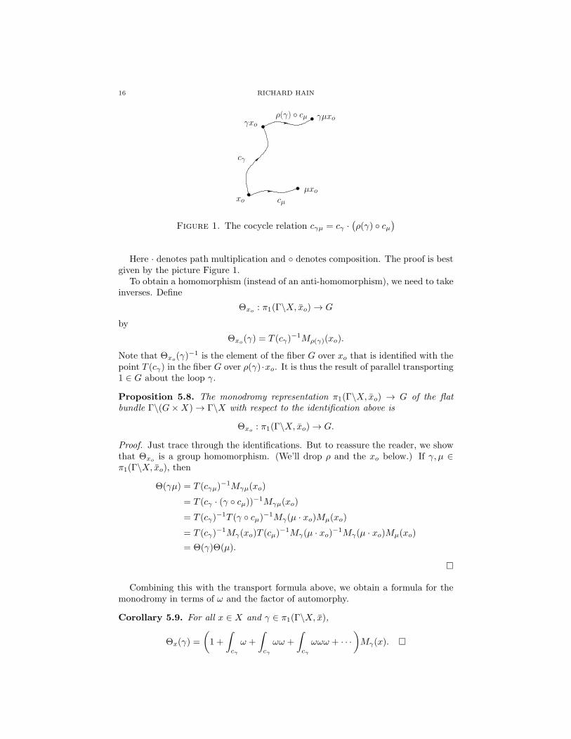
Lemma 5.7. If γ, µ ∈ π1(Γ\X, xo), then cγµ = cγ ·(ρ(γ) cµ
).
16 RICHARD HAIN
cγ
cµxo
γxo
µxo
γµxoρ(γ) cµ
Figure 1. The cocycle relation cγµ = cγ ·(ρ(γ) cµ
)
Here · denotes path multiplication and denotes composition. The proof is bestgiven by the picture Figure 1.
To obtain a homomorphism (instead of an anti-homomorphism), we need to takeinverses. Define
Θxo : π1(Γ\X, xo) → G
by
Θxo(γ) = T (cγ)−1Mρ(γ)(xo).
Note that Θxo(γ)−1 is the element of the fiber G over xo that is identified with the
point T (cγ) in the fiber G over ρ(γ) ·xo. It is thus the result of parallel transporting1 ∈ G about the loop γ.
Proposition 5.8. The monodromy representation π1(Γ\X, xo) → G of the flatbundle Γ\(G×X) → Γ\X with respect to the identification above is
Θxo : π1(Γ\X, xo) → G.
Proof. Just trace through the identifications. But to reassure the reader, we showthat Θxo is a group homomorphism. (We’ll drop ρ and the xo below.) If γ, µ ∈π1(Γ\X, xo), then
Θ(γµ) = T (cγµ)−1Mγµ(xo)
= T (cγ · (γ cµ))−1Mγµ(xo)
= T (cγ)−1T (γ cµ)−1Mγ(µ · xo)Mµ(xo)
= T (cγ)−1Mγ(xo)T (cµ)
−1Mγ(µ · xo)−1Mγ(µ · xo)Mµ(xo)
= Θ(γ)Θ(µ).
Combining this with the transport formula above, we obtain a formula for themonodromy in terms of ω and the factor of automorphy.
Corollary 5.9. For all x ∈ X and γ ∈ π1(Γ\X, x),
Θx(γ) =
(1 +
∫
cγ
ω +
∫
cγ
ωω +
∫
cγ
ωωω + · · ·)Mγ(x).
NOTES ON THE UNIVERSAL ELLIPTIC KZB CONNECTION 17
Part 2. The Universal Elliptic KZB Connection
6. The Bundle PPP over E ′
Before we define the universal elliptic KZB connection, we need to define thebundle PPP over E ′ on which it lives.
6.1. The flat bundle PPPtop. The bundle PPP with the KZB connection will be the
de Rham realization of a topological local system PPPtop. To provide context, we firstconstruct it.
Denote by Y the universal covering space of E ′. This is also the universal coveringspace of E ′
h =(C× h)−Λh. Choose a base point [Eo, xo] of E ′ and a lift yo of it to
Y . This determines an isomorphism of Aut(Y/E ′) with π1(E ′, [Eo, xo]).Denote the unipotent completion of π1(E
′o, xo) over C by Po. The natural action
π1(E ′, [Eo, xo])× π1(E′o, xo) → π1(E
′o, xo), (g, γ) 7→ gγg−1
determines a left action of π1(E ′, [Eo, xo]) on Po. We can therefore form the quotient
π1(E ′, [Eo, xo])\(Po × Y
)
by the diagonal π1(E ′, [Eo, xo])-action. This is a flat right principal Po-bundle which
we shall denote by PPPtop → E ′. Its fiber over [E, x] is naturally isomorphic to theunipotent completion of π1(E
′, x).Since the Lie algebra po of Po can be viewed as a group with multiplication
defined by the Baker-Campbell-Hausdorff formula, we can (and will) view PPPtop asa local system of Lie algebras. (Cf. the comment following Prop. 2.1.)
6.2. The bundle PPP. Here we construct a bundle PPP over E on which the universalelliptic KZB connection lives. Its fiber over each point of E ′ is the Lie algebra
p := L(t, a)∧.
Denote the corresponding group exp p by P . It is prounipotent. The universalelliptic KZB connection on it is constructed in Section 9. It is flat. In Section 14we will prove that it is isomorphic to the flat bundle PPP.
The bundle PPP will be constructed as the quotient of p × C × h by a lift of theaction of SL2(Z) ⋉ Z2 on C× h to p× C× h.
The (completed) universal enveloping algebra of p is the power series algebraC〈〈t, a〉〉. The adjoint action defines the ring homomorphism
C〈〈t, a〉〉 → End p
that takes f(t, a) to f(adt, ada) ∈ End p. This restricts to a homomorphismC〈〈t, a〉〉× → Aut p.
We use the notation of Section 3. Take G = Γ := SL2(Z) ⋉ Z2, X = C× h, andV = p. Note that Γ acts on p×X via the projection Γ → SL2(Z) using the factorof automorphy Mγ(τ) defined in (6.1).
The bundle PPP is defined using factors of automorphy Mγ(ξ, τ) which live in thegroup SL2(R)⋉C〈〈t, a〉〉×, where SL2(R) acts on C〈〈t, a〉〉 via its left action on thegenerators via the factor of automorphyMγ(τ) defined in Example 3.4. Specifically,Mγ(τ) is defined by
(6.1) Mγ(τ) :
a 7→ (cτ + d)−1a+ 2πict
t 7→ (cτ + d)t.
18 RICHARD HAIN
The general factor of automorphy is defined by
(6.2) Mγ(ξ, τ) =
Mγ(τ) e
(cξt
cτ+d
)γ ∈ SL2(Z);
e(−mt) (m,n) ∈ Z2.
Here e(u) := exp(2πiu). This is a factor of automorphy for Γ as
e(cξt−mt) Mγ(τ) = Mγ
(ξ + (m,n)γ(τ, 1)T , τ
) e(−mt),
where γ ∈ SL2(Z) and (m,n) ∈ Z2.6
Proposition 6.1. This is a well-defined factor of automorphy.
Proof. The first task is to show that M is well-defined on Γ× C × h — that is, itis compatible with the relation in Γ = SL2(Z)⋉ Z2. This relation is
(m,n) γ = γ (m,n)(·γ),where γ ∈ SL2(Z), denotes composition in Γ and · denotes the right action ofSL2(Z) on Z2. If
γ =
(a bc d
)
then we have to show that
e(−mt) Mγ(ξ, τ) = Mγ(ξ + (m,n)γ(τ, 1)T , τ) e(− (ma+ nc)t
).
SinceMγ(τ) e(φ) = e(Mγ(τ) · φ) Mγ(τ)
for all φ ∈ C〈〈t, a〉〉, and since Mγ(τ) : t 7→ (cτ + d)t (see above), we have
e(−mt) Mγ(τ) =Mγ(τ) e( −mt
cτ + d
).
Thus, the left-hand side expands to
e(−mt) Mγ(ξ, τ) = e(−mt) Mγ(τ) e(
cξt
cτ + d
)
=Mγ(τ) e(cξt−mt
cτ + d
)
The right-hand side expands to
Mγ(ξ + (ma+ nc)τ + (mb + nd), τ) e(− (ma+ nc)t
)
=Mγ(τ) e(c(ξ + (ma+ nc)τ + (mb+ nd)
)t
cτ + d
) e(− (ma+ nc)t
)
=Mγ(τ) e(cξt−mt
cτ + d
),
which equals the left-hand side. It follows that M is a well-defined function onΓ× C× h.
Since M defines a homomorphism Z2 → Q〈〈t〉〉×, to complete the proof we need
only check that the restriction of M to SL2(Z) × C× h is a factor of automorphy.We will use the fact that Mγ(τ) is a factor of automorphy.
6Denote left multiplication by φ ∈ C〈〈t,a〉〉 by Lφ. For M ∈ AutH, we have M LM−1φ =
Lφ M . In particular, Mγ(τ) Lt/(cτ+d) = Lt Mγ(τ).
NOTES ON THE UNIVERSAL ELLIPTIC KZB CONNECTION 19
Let
γ1 =
(a bc d
), γ2 =
(p qr s
)and γ1γ2 =
(e fg h
).
Set (ξ′, τ ′) = γ2(ξ, τ) = (ξ/(rτ + s), γ2τ). Then
Mγ1(ξ′, τ ′)Mγ2
(ξ, τ) =Mγ1(γ2τ) e
(cξ′t
cτ ′ + d
)Mγ2
(τ) e(
rξt
rτ + s
)
=Mγ1(γ2τ)Mγ2
(τ) e(
cξ′t
(cτ ′ + d)(rτ + s)
) e(
rξt
rτ + s
)
=Mγ1γ2(τ) e
(cξt
(rτ + s)(c(pτ + q) + d(rτ + s)
) + rξt
rτ + s
)
=Mγ1γ2(τ) e
((c+ r(gτ + h)
)ξt
(rτ + s)(gτ + h)
)
=Mγ1γ2(τ) e
(gξt
gτ + h
)
= Mγ1γ2(ξ, τ).
Remark 6.2. The bundle PPP is a bundle of free Lie algebras. Its quotient by thecommutator subalgebra of each fiber is the bundle over h with framing t, a andfactor of automorphyMγ(τ). So it is isomorphic to H by Example 3.4, as it shouldbe.
7. Eisenstein Series and Bernoulli Numbers
Define the Bernoulli numbers Bn by
x
ex − 1=
∞∑
n=0
Bnxn
n!.
Recall that B0 = 1, B1 = −1/2 and that B2k+1 = 0 when k > 0.There are several ways to normalize Eisenstein series G2k : h → C. We will use
the normalization used by Zagier [33]:
G2k(τ) =1
2
(2k − 1)!
(2πi)2k
∑
λ∈Z⊕Zτλ6=0
1
λ2k= −B2k
4k+
∞∑
n=1
σ2k−1(n)qn,
(properly summed when k = 1), where q = e(τ) and σk(n) =∑
d|n dk. In particular
G2k|q=0 = −B2k
4k=
(2k − 1)!
(2πi)2kζ(2k).
When k > 1, G2k is a modular form for SL2(Z) of weight 2k:
Gk(γτ) = (cτ + d)kGk(τ), γ ∈ SL2(Z).
And G2 satisfies
G2(γτ) = (cτ + d)2G2(τ) + ic(cτ + d)/4π.
(Cf. [33, p. 457], bottom of page, and [33, p. 459], near bottom of page.)The role of G2(τ) in this work should be clarified by the following result, which
follows from the transformation law for G2 above.
20 RICHARD HAIN
Lemma 7.1. If SL2(Z) acts on C × h by γ : (ξ, τ) 7→(ξ/(cτ + d), γτ
), then the
formdξ
ξ− 2 · 2πiG2(τ) dτ
is SL2(Z)-invariant.
This 1-form represents a generator of H1(L′−1,Z(1))
∼= Z.
7.1. Some useful identities. The following well-known identities are used laterin the paper. Since
1
2coth
(u/2
)=
1
2
eu/2 + e−u/2
eu/2 − e−u/2=
1
2
eu + 1
eu − 1=
1
2+
1
u
u
eu − 1=
∞∑
m=0
B2m
(2m)!u2m−1,
we have
(7.1)1
u− u/4
sinh2(u/2)=
1
u+u
2
d
ducoth
(u/2) =
∞∑
m=1
(2m− 1)B2m
(2m)!u2m−1.
Rearranging gives the useful alternative form
(7.2)
∞∑
m=0
(2m− 1)B2m
(2m)!u2m−1 = − u/4
sinh2(u/2).
8. The Jacobi Form F (ξ, η, τ)
There are two versions of the function F (u, v, τ), one used by Levin-Racinet [24],the other by Zagier [33].7 Denote them by F (ξ, η, τ) and FZag(u, v, τ), respectively.Zagier’s function is defined by
FZag(u, v, τ) :=θ′(0, τ)θ(u + v, τ)
θ(u, τ)θ(v, τ),
where θ is the classical theta function
θ(u, τ) :=∑
n∈Z
(−1)nq12(n+ 1
2)2e(n+
12)u, q = e(τ)
and θ′ is its derivative with respect to u.Their periodicity properties imply that u = 2πiξ, v = 2πiη. Since
F (ξ, η, τ) =1
ξ+
1
ηmod holomorphic functions
and
FZag(u, v, τ) =1
u+
1
vmod holomorphic functions
near the origin, it follows that
F (ξ, η, τ) = 2πiFZag(2πiξ, 2πiη, τ).
It satisfies the symmetry condition
F (ξ, η, τ) = F (η, ξ, τ) = −F (−ξ,−η, τ).7Calaque-Enriquez-Etingof [3] do not explicitly use the Jacobi form F . However, their con-
nection is expressed in terms of the function k(z, x|τ), which is FZag(z, x, τ) − 1/x. See theirSection 1.2.
NOTES ON THE UNIVERSAL ELLIPTIC KZB CONNECTION 21
8.1. Expansions. We use the formulas in [33], but write them using F in place ofFZag.8
Set q = exp(2πiτ). Then
(8.1) F (ξ, η, τ) = πi[coth(πiξ)+ coth(πiη)
]+4π
∞∑
n=1
(∑
d|n
sin[2π(ndξ+ dη
)])qn.
(8.2) F (ξ, η, τ) =1
ξ+
1
η− 2
∞∑
r,s=0
(2πi)1+maxr,s
(∂
∂τ
)minr,s
G|r−s|+1(τ)ξr
r!
ηs
s!.
8.2. Derivatives. Differentiating these with respect to η yields:
1
η+ η
∂F
∂η(ξ, η, τ) = −2
∑
r≥0s≥1
(2πi)1+maxr,s
(∂
∂τ
)minr,s
G|r−s|+1(τ)ξr
r!
ηs
(s− 1)!
=
(1
η− (πi)2η
sinh2(πiη)
)+ 8π2η
∞∑
n=1
(∑
d|n
d cos[2π(ndξ + dη
)])qn.
(8.3)
Comparing the result of differentiating this with respect to ξ and (8.2) withrespect to τ , we obtain the heat equation:
2πi∂F
∂τ(ξ, η, τ) =
∂2F
∂ξ∂η(ξ, η, τ).
8.3. Elliptic and modularity properties. The elliptic property, [33, p. 456] is:
(8.4) F (ξ +mτ + n, η, τ) = e(−mη)F (ξ, η, τ) (m,n) ∈ Z2.
Here, as previously, e(x) = exp(2πix). Zagier states a more general form of this,which follows from this one using the symmetry property of F (ξ, η, τ).
The modularity property is:
(8.5) F (ξ/(cτ + d), η/(cτ + d), γτ) = (cτ + d)e(cξη/(cτ + d)
)F (ξ, η, τ).
In particular
F (ξ, η, τ + 1) = F (ξ, η, τ) = F (ξ + 1, η, τ).
Proposition 8.1. The function F induces a meromorphic section of the line bundleN → E ×M1,1
E that was constructed in Example 3.2. The divisor of the section is
[Γι] − [01] − [02], where Γι is the graph in E × E of the involution ι that takes apoint of E to its inverse.
Proof. Since F (ξ, η, τ) is meromorphic on C2 for each τ ∈ h, divF has no verticalcomponents over M1,1. The polar locus of F over M1,1 contains [01] + [02] withmultiplicity one on every fiber over M1,1. The zero divisor of F over M1,1 contains[Γι] with multiplicity one on the generic fiber over M1,1. Since the class of divF inH2(E2
τ ) is constant and since divF has no vertical components, it suffices to showthat the class of divF is exactly [Γι]− [01]− [02] on an open set of fibers and alsoover q = 0.
8Note the conflict in notation: Zagier sets ξ = expu and η = exp v, which conflicts with thevariables (ξ, η) used by Levin-Racinet: 2πi(ξ, η) = (u, v). See [33, p. 455].
22 RICHARD HAIN
Identity (8.1) implies that
1
πiF (ξ, η)|q=0 =
w + 1
w − 1+u+ 1
u− 1
where w = exp(2πiξ) and u = exp(2πiη). The coordinates on the normalization ofE0 × E0 are (w, u). The identity sections are w = 1 and u = 1. The involution isgiven by w = 1/w. It is easily checked that
w + 1
w − 1+u+ 1
u− 1= 0
implies that wu = 1. It follows that the restriction of divF to E0 × E0 is [Γι] −[01] − [02]. But this implies that the divisor of F is [Γι]− [01]− [02] on all nearbyfibers. The result follows.
This result can also be proved using the formula for F in terms of theta functions.
8.4. The Weierstrass ℘ function. Recall that
℘(z, τ) =1
z2+
∑
λ∈Z⊕Zτλ6=0
[1
(z − λ)2− 1
λ2
].
The next result follows from the standard identity
℘(z, τ) =1
z2+
∞∑
m=2
(2m− 1)
( ∑
λ∈Z⊕Zτλ6=0
1
λ2m
)z2m−2
=1
z2+
∞∑
m=2
2(2πi)2m
(2m− 2)!G2m(τ)z2m−2
=1
z2+
∞∑
m=1
2(2πi)2m+2
(2m)!G2m+2(τ)z
2m.
Lemma 8.2. Suppose that x, y are commuting indeterminants. Then
1
2
xy
x+ y
((℘(x, τ) − 1
x2)−(℘(y, τ)− 1
y2))
=∑
m≥1
(2πi)2m+2
(2m)!G2m+2(τ)
∑
j+k=2m+1j,k>0
(−1)jxjyk
in the ring O(h)[[x, y]] of formal power series with coefficients in O(h).
8.5. The addition formula. The following identity is used in the proof of theintegrability of the elliptic KZB connection.
Proposition 8.3 (Addition Formula).
F (ξ, η1, τ)∂F
∂η(ξ, η2, τ)− F (ξ, η2, τ)
∂F
∂η(ξ, η1, τ)
= F (ξ, η1 + η2, τ)(℘(η1, τ) − ℘(η2, τ)
).
NOTES ON THE UNIVERSAL ELLIPTIC KZB CONNECTION 23
9. The Universal Elliptic KZB Connection
This is a Γ-invariant flat connection constructed by Calaque, Enriquez andEtingof [3] and by Levin and Racinet [24] on the bundle
(9.1) p× C× h → C× h.
So it descends to a flat connection on the bundle PPP → E ′. It has regular singularitiesalong the universal lattice:
Λh := (mτ + n, τ) ∈ C× h.It therefore descends to a meromorphic connection on the bundle PPP → E withregular singularities along the zero-section. In Section 12 we show that the naturalextension of this connection to the q-disk has regular singularities along the nodalcubic.
In this section we will follow Levin-Racinet (with modifications).
9.1. Derivations. We have already explained the algebra homomorphism
C〈〈t, a〉〉 → End p, f(t, a) 7→ x 7→ f(t, a) · x,where f(t, a) · x := f(adt, ada)(x). We will view p as a Lie subalgebra of Der pvia the adjoint action ad : p → Der p, which is an inclusion as p has trivial center.Every derivation δ can be written uniquely in the form
δ = δ(a)∂
∂a+ δ(t)
∂
∂t.
Consequently, there is a linear isomorphism
p∂
∂t⊕ p
∂
∂a
≃−→ Der p.
9.2. The formula. The connection is defined by a 1-form
ω ∈ Ω1(C× h, log Λ)⊗End p.
via the formula
∇f = df + ωf
where f : C× h → p is a (locally defined) section of (9.1). Specifically,
ω =1
2πidτ ⊗ a
∂
∂t+ ψ + ν
where
ψ =∑
m≥1
((2πi)2m+1
(2m)!G2m+2(τ)dτ ⊗
∑
j+k=2m+1j,k>0
(−1)j[adjt(a), adk
t(a)]
∂
∂a
)
and
ν = tF (ξ, t, τ) · a dξ + 1
2πi
(1
t+ t
∂F
∂t(ξ, t, τ)
)· a dτ.
Note that each term takes values in Der p. Later we will show that its restrictionto a punctured first order neighbourhood of the identity section takes values in asmaller subalgebra.
24 RICHARD HAIN
Remark 9.1. Each term of the lower central series of PPP is preserved by the connec-tion. The connection thus induces a connection on the bundle of abelianizations,which is isomorphic to H (cf. Remark 6.2). Example 5.2 implies that this inducedconnection on H is the natural connection.
9.3. Modularity. Recall that Γ = SL2(Z)⋉ Z2. In this section we shall prove:
Proposition 9.2. The universal elliptic KZB connection is SL2(Z)⋉Z2-invariant.That is,
γ∗ω = Ad(Mγ
)· ω − dMγM
−1γ
for all γ ∈ SL2(Z) ⋉ Z2.
It suffices to check that the connection is invariant under Z2 and SL2(Z). Theseare proved in the two following subsections.
9.3.1. Ellipticity: invariance under Z2.
Lemma 9.3. For all δ ∈ Der p we have
e(−mt) · δ = δ +1− e(−m adt)
adtδ(t).
Proof. For all x ∈ p(e(−mt) · δ
)(x) = e(−mt)δ
(e(mt)(x)
)(Equation 4.1)
= e(−mt)δ(e(mt))(x) + e(−mt)e(mt)δ(x)
= δ(x) +1− e(−m adt)
2πim adtδ(2πimt) · x (Lemma 4.2)
= δ(x) +1− e(−m adt)
adtδ(t) · x
=
(δ +
1− e(−m adt)
adtδ(t)
)(x).
Corollary 9.4. If (m,n) ∈ Z2, then
(m,n)∗(
1
2πia∂
∂tdτ
)− e(−mt) ·
(1
2πia∂
∂tdτ
)= − 1
2πi
1− e(−mt)
t(a)dτ.
Proof. Apply the previous lemma with δ = a ∂∂t .
Corollary 9.5. If a, b ∈ N, then
e(−mt) · [ta · a, tb · a] ∂∂a
= [ta · a, tb · a] ∂∂a.
Proof. This follows directly from the previous lemma as the derivation
[ta · a, tb · a] ∂∂a
annihilates t.
Corollary 9.6. If (m,n) ∈ Z2, then (m,n)∗ψ = e(−mt) · ψ = ψ.
Lemma 9.7. For all (m,n) ∈ Z2
(m,n)∗ν − e(−mt) · ν =1
2πi
1− e(−m adt)
adt(a)dτ.
NOTES ON THE UNIVERSAL ELLIPTIC KZB CONNECTION 25
Proof. Write ν = ν1 + ν2, where
ν1 = tF (ξ, t, τ) · a dξ and ν2 =1
2πi
(1
t+ t
∂F
∂t(ξ, t, τ)
)· a dτ.
Then
(m,n)∗ν1 − e(−mt) · ν1= tF (ξ +mτ + n, t) · a d(ξ +mτ + n)− te(−mt)F (ξ, t) · a dξ= te(−mt)F (ξ, t) · a (dξ +mdτ) − te(−mt)F (ξ, t) · a dξ= mte(−mt)F (ξ, t) · a dτ.
Note that
∂F
∂t(ξ +mτ + n, t) =
∂
∂t
(e(−mt)F (ξ, t)
)
= e(−mt)∂F
∂t(ξ, t)− 2πime(−mt)F (ξ, t).
Thus
2πi((m,n)∗ν2 − e(−mt) · ν2
)
=
(1
t+ t
∂F
∂t(ξ +mτ + n, t, τ)
)· a dτ − e(−mt)
(1
t+ t
∂F
∂t(ξ, t, τ)
)· a dτ
= −2πimte(−mt)F (ξ, t) · a dτ + 1
t
(1− e(−mt)
)· a dτ.
If (m,n) ∈ Z2, then the results above imply that
(m,n)∗ω = e(−mt) · ω(ξ, τ).Since e(−mt) does not depend on (ξ, τ), de(−mt) = 0 and ω is invariant under Z2.
9.3.2. Modularity: invariance under SL2(Z). Let
γ =
(a bc d
)∈ SL2(Z).
Recall that Mγ(τ) is defined by
a 7→ (cτ + d)−1a+ 2πict
t 7→ (cτ + d)t.(9.2)
Its inverse is the linear map
a 7→ (cτ + d)a− 2πict
t 7→ (cτ + d)−1t.(9.3)
Lemma 9.8. If γ ∈ SL2(Z) and a, b ∈ N, then
e(cξt/(cτ + d)) · [adat(a), adb
t(a)]
∂
∂a= [ada
t(a), adb
t(a)]
∂
∂a.
Proof. This follows from (4.1) as the derivation δ = [adat(A), adb
t(A)] ∂
∂a vanishes ont.
26 RICHARD HAIN
Lemma 9.9. If γ ∈ SL2(Z) and a, b ∈ N, then
Ad(Mγ(τ))[adat(A), adb
t(a)]
∂
∂a= (cτ + d)a+b−1[ada
t(A), adb
t(A)]
∂
∂a.
Proof. Set δ = [adat(a), adb
t(a)] ∂
∂a . Since Mγ(τ)−1(t) = (cτ + d)−1t, δ M−1
γ (t) =
0. Consequently, Ad(Mγ(τ))δ is of the form f(t, a) ∂∂a . The coefficient f(t, a) is
computed as follows:
Ad(Mγ(τ))δ(a)
=Mγ(τ) δ Mγ(τ)−1(a)
=Mγ(τ) δ((cτ + d)a− 2πict
)
= (cτ + d)Mγ(τ)([ada
t(a), adb
t(a)]
)
= (cτ + d)a+b+1[adat
((cτ + d)−1a+ 2πict
), adb
t
((cτ + d)−1a+ 2πict
)]
= (cτ + d)a+b−1[adat(a), adb
t(a)].
Corollary 9.10. If γ ∈ SL2(Z), then γ∗ψ = Ad(Mγ)ψ.
Proof. This follows as, for each k ≥ 1, the expression
G2k+2(τ)dτ ⊗∑
a+b=2k+1a,b>0
[adat(a), adb
t(a)]
∂
∂a
is multiplied by (cτ + d)2k by both γ∗ and Mγ(ξ, τ).
Lemma 9.11. Set ν1 = tF (ξ, t, τ) · adξ. Then
γ∗ν1 − Mγ(ξ, τ)ν1 = −2πict dξ − cξt
cτ + de(cξt)F (ξ, (cτ + d)t, τ) · a dτ.
Proof. First,
Mγ(ξ, τ)ν1 = Mγ(ξ, τ)[tF (ξ, t, τ) · a
]dξ
= e(cξt)(cτ + d)tF (ξ, (cτ + d)t, τ) ·((cτ + d)−1a+ 2πict
)dξ
= e(cξt)tF (ξ, (cτ + d)t, τ) · a dξ + 2πict dξ.
as the value of tF (ξ, (cτ + d)t, τ) at t = 0 is (cτ + d)−1. This and the modularproperty of F (ξ, t, τ) then yield:
γ∗ν1 = tF (ξ/(cτ + d), t, γτ) · aγ∗dξ
= (cτ + d)te(cξt)F (ξ, (cτ + d)t, τ) · a(
dξ
cτ + d− cξdτ
(cτ + d)2
)
= te(cξt)F (ξ, (cτ + d)t, τ) · a(dξ − cξdτ
cτ + d
)
= Mγ(ξ, τ)ν1 − 2πict dξ − cξt
cτ + de(cξt)F (ξ, (cτ + d)t, τ) · a dτ.
As a special case of the general formula, we have:
NOTES ON THE UNIVERSAL ELLIPTIC KZB CONNECTION 27
Lemma 9.12. In Der p we have:
e(cξ adt)
(1
2πia∂
∂t
)=
1
2πia∂
∂t+
1
2πi
1− e(cξt)
t· a.
Lemma 9.13. Set
ν2 =1
2πi
(1
t+ t
∂F
∂t(ξ, t, τ)
)· a dτ.
Then
γ∗ν2 − Mγ(ξ, τ)ν2 =1
2πi
1− e(cξt)
t· a dτ
(cτ + d)2
+cξt
cτ + de(cξt)F (ξ, (cτ + d)t, τ) · a dτ.
Proof. First note that the modularity property of F (ξ, t, τ) implies that
∂F
∂t(ξ/(cτ + d), t, γτ)
= (cτ + d)∂
∂t
[e(cξt)F (ξ, (cτ + d)t, τ)
]
= (cτ + d)e(cξt)[cξF (ξ, (cτ + d)t, τ) + (cτ + d)
∂F
∂t(ξ, (cτ + d)t, τ)
].
Thus
2πiγ∗ν2 =
(1
t+ t
∂F
∂t(ξ/(cτ + d), t, γτ)
)· a d
(aτ + b
cτ + d
)
=
(1
t+ (cτ + d)2e(cξt)t
∂F
∂t(ξ, (cτ + d)t, τ)
+ cξt(cτ + d)e(cξt)F (ξ, (cτ + d)t, τ)
)· a dτ
(cτ + d)2.
Since
Mγ(ξ, τ)(t) = (cτ + d)t and Mγ(ξ, τ)(a) = e(cξt) · a/(cτ + d) + 2πict
we have
2πiMγ(ξ, τ)ν2
=
(1
(cτ + d)t+ (cτ + d)t
∂F
∂t(ξ, (cτ + d)t, τ)
)·(e(cξt) · a/(cτ + d) + 2πict
)dτ
= e(cξt)
(1
t+ (cτ + d)2t
∂F
∂t(ξ, (cτ + d)t, τ)
)· a dτ
(cτ + d)2
as 1η + η ∂F
∂η (ξ, η, τ) is holomorphic in η and vanishes at η = 0 by (8.3).
The previous lemma implies that
(e(cξ adt)− 1
)( 1
2πia∂
∂t
)=
1
2πi
(1− e(cξt)
t
)· a.
Now assemble the pieces to obtain the result.
Combining the last two computations, we obtain:
28 RICHARD HAIN
Corollary 9.14. For all γ ∈ SL2(Z),
γ∗ν − Mγν =1− e(cξt)
2πit· a dτ
(cτ + d)2− 2πict dξ.
Lemma 9.15. For all γ ∈ SL2(Z),
dMγM−1γ = e(cξt) ·
(dMγM
−1γ
)+ 2πict dξ.
Proof. Since Mγ(ξ, τ) = e(cξt)Mγ(τ), we have
dMγM−1γ = d
(e(cξt)Mγ
)M−1
γ e(−cξt)=(e(cξt)dMγ + 2πicte(cξt)Mγdξ
)M−1
γ e(−cξt)= e(cξt) ·
(dMγM
−1γ
)+ 2πict dξ.
Lemma 9.16. For all γ ∈ SL2(Z), we have
γ∗(
1
2πia∂
∂tdτ
)−Mγ
(1
2πia∂
∂tdτ
)+ dMγM
−1γ = 0.
Proof. This is best done using matrices with respect to the basis a, t of H . Wehave
1
2πia∂
∂tdτ =
1
2πi
(0 10 0
)dτ
and
Mγ(τ) =
((cτ + d)−1 0
2πic cτ + d
), Mγ(τ)
−1 =
(cτ + d 0−2πic (cτ + d)−1
).
So
dMγM−1γ =
(−c(cτ + d)−2 0
0 c
)(cτ + d 0−2πic (cτ + d)−1
)dτ
=
(−c 0
−2πic2(cτ + d) c
)dτ
cτ + d
and
Mγ
(1
2πia∂
∂tdτ
)=
1
2πi
((cτ + d)−1 0
2πic cτ + d
)(0 10 0
)(cτ + d 0−2πic (cτ + d)−1
)dτ
=1
2πi
(−2πic (cτ + d)−1
−(2πic)2(cτ + d) 2πic
)dτ
cτ + d
=1
2πi
(0 10 0
)dτ
(cτ + d)2+
(−c 0
−2πic2(cτ + d) c
)dτ
cτ + d
= γ∗(
1
2πia∂
∂tdτ
)+ dMγM
−1γ .
NOTES ON THE UNIVERSAL ELLIPTIC KZB CONNECTION 29
Final computation: For all γ ∈ SL2(Z), we have:
γ∗ω − Mγω + dMγM−1γ
= γ∗(ν +
a
2πi
∂
∂tdτ
)− Mγ
(ν +
a
2πi
∂
∂tdτ
)+ e(cξt) ·
(dMγM
−1γ
)+ 2πict dξ
= γ∗(
a
2πi
∂
∂tdτ
)+
1− e(cξt)
2πit· a dτ
(cτ + d)2− e(cξt) ·Mγ
(a
2πi
∂
∂tdτ
)
+ e(cξt) ·(dMγM
−1γ
)
= e(cξt) ·(γ∗(
1
2πia∂
∂tdτ
)−Mγ
(1
2πia∂
∂tdτ
)+ dMγM
−1γ
)
= 0.
9.4. Integrability.
Proposition 9.17. The 1-form ω is closed.
Proof. It is clear that
d
(1
2πidτ ⊗ a
∂
∂t+ ψ
)= 0
as these terms do not depend upon ξ. The heat equation implies that
2πi dν = 2πi adt dF (ξ, adt, τ)(a) ∧ dξ + d
(1
adt+ adt
∂F
∂t(ξ, adt, τ)
)(a) ∧ dτ
= adt
(2πi
∂F
∂τ(ξ, adt, τ) −
∂2F
∂ξ∂t(ξ, adt, τ)
)(a)dτ ∧ dξ
= 0,
so that dω = 0.
The proof of the vanishing of [ω, ω] is quite involved. For this we employ theelegant calculus developed by Levin and Racinet in [24, §3.1].
9.4.1. The Levin-Racinet calculus. For U, V ∈ L(a, t)∧, define
xrys (U, V ) = [tr · U, ts · V ].
This extends linearly to an action f(x, y) (U, V ) of polynomials and power seriesf(x, y) in commuting indeterminants on ordered pairs of elements of L(t, a). WhenU and V are equal, one has the identity f(x, y) (U,U) = −f(y, x) (U,U), so that
(9.4) f(x, y) (U,U) =1
2
(f(x, y)− f(y, x)
) (U,U).
As an example of how this notation is used, note that Lemma 8.2 implies that
(9.5) 2πiψ =1
2
xy
x+ y
(℘(x)− 1
x2− ℘(y) +
1
y2) (a, a) ∂
∂a⊗ dτ.
Two more identities will be needed in the proof of the vanishing of [ω, ω].
Lemma 9.18. Suppose that U, V ∈ L(t, a)∧.
(i) (Jacobi identity) If f(x, y) ∈ C[[x, y]], then
adt(f(x, y) (U, V )
)= (x+ y)f(x, y) (U, V ).
30 RICHARD HAIN
(ii) If δ is a continuous derivation of C〈〈t, a〉〉 and g(x) ∈ C[[x]], then
δ(g(adt)V
)= g(adt)δ(V ) +
(g(x+ y)− g(y)
x
) (δ(t), V ).
Proof. The first identity encodes the Jacobi identity and is left as an easy exercise.To prove the second, note that both sides are linear in g, so that, by continuity,it suffices to prove the result when g is a monomial xn. This holds trivially whenn ≤ 1. The general case follows by induction using the Jacobi identity.
9.5. Integrability. The following computation completes the proof of integrabil-ity.
Lemma 9.19. The 2-form [ω, ω] vanishes, so that ω is integrable.
Proof. Note that
πi [ω, ω] =
[dτ ⊗ a
∂
∂t+ 2πi ψ
+ dτ ⊗(
1
adt+ adt
∂F
∂t(ξ, adt, τ)
)(a), adt F (ξ, adt, τ)(a) ⊗ dξ
].
The expression (9.5) implies that the coefficient of dτ ∧ dξ is
[a∂
∂t, tF (t)(a)] +
1
2
[ xy
x+ y
(℘(x) − 1
x2− ℘(y) +
1
y2) (a, a) ∂
∂a, tF (t)(a)
]
+[1t+ tF ′(t)(a), tF (t)(a)
]
where F (z) denotes F (ξ, z, τ) and F ′(z) denotes ∂F/∂z(ξ, z, τ). We’ll computethese three terms, one at a time.
Since [δ, adv] = adδ(v), Lemma 9.18 and equation (9.4) imply that the first termis
[a∂
∂t, tF (t) · a] =
((x+ y)F (x+ y)− yF (y)
x
) (a, a)
=1
2
((y2 − x2
xy
)F (x+ y)− y
xF (y) +
x
yF (x)
) (a, a).
The identity [δ, adv] = adδ(v) and the Jacobi identity (Lemma 9.18) imply thatthe second term is
1
2adtF (t)
(xy
x+ y
(℘(x)− 1
x2− ℘(y) +
1
y2
) (a, a)
)
=1
2xyF (x+ y)
(℘(x)− 1
x2− ℘(y) +
1
y2
) (a, a)
=1
2
((x2 − y2
xy
)F (x+ y) + xy(℘(x) − ℘(y))F (x+ y)
) (a, a)
NOTES ON THE UNIVERSAL ELLIPTIC KZB CONNECTION 31
The addition formula, Proposition 8.3, implies that the third term is((1
x+ xF ′(x)
)yF (y)
) (a, a)
=( yxF (y) + xyF ′(x)F (y)
) (a, a)
=1
2
(yxF (y)− x
yF (x) + xy
(F ′(x)F (y) − F ′(y)F (x)
)) (a, a)
=1
2
(yxF (y)− x
yF (x) − xy
(℘(x)− ℘(y)
)F (x+ y)
) (a, a).
These three terms clearly sum to 0.
Part 3. Hodge Theory and Applications
The main goal of this section is to show that the elliptic KZB connection underliesan admissible variation of mixed Hodge structure (MHS) over E ′ = M1,2 and toshow that this variation is isomorphic to the variation of MHS whose fiber over[E, x] is the Lie algebra of the unipotent fundamental group of (E′, x). We use thisto show that the periods of the limit MHS on the fiber of PPP over [E∂/∂q, ∂/∂w]are multizeta values and to derive an explicit formula for the natural morphism ofMHS
πun1 (P1 − 0, 1,∞, ∂/∂w) → πun
1 (E′∂/∂q, ∂/∂w).
As preparation, we show that the KZB connection extends to a meromorphicconnection overM1,2 with regular singularities and pronilpotent monodromy aboutthe boundary divisors. To fill a gap in the literature, we prove, in Section 14, thatthe local system associated to the universal elliptic KZB connection onPPP is the localsystem PPPtop. It can be used to prove the analogous result for the KZB connectionover M1,1+n. This complements results in [24, §4] and [3, §4.3].
Throughout, p = L(t, a)∧ and P is the corresponding prounipotent group. Set
Der0 p = δ ∈ Der p : δ([t, a]) = 0.This is the infinitesimal analogue of the mapping class group Γ1,~1.
The reader is assumed to be familiar with the basics of Deligne’s theory ofmixed Hodge structures [7]. A good introductory reference is the book [30] bySteenbrink and Peters. Another good introductory reference is Carlson’s paper [4].An exposition of the construction of the mixed Hodge structure on the unipotentfundamental group of a smooth variety can be found in [11].
10. Extending PPP to M1,2
The punctured universal elliptic curve E ′ is isomorphic to M1,2 and is the com-
plement of a normal crossing divisor in M1,2. This divisor has two components:the zero section and the nodal cubic. The flat bundle P over E ′ has prounipotentmonodromy about each, and thus extends naturally to a bundle over M1,2 withregular singularities and (pro) nilpotent residues along each component.
This extension is easily described. First, the complement of the Tate curve inM1,2 is the universal elliptic curve E , which is a quotient of C× h. The bundle PPPdefined in Section 6.2 is defined over E , not just over E ′. We take this to be theextension across the zero section.
32 RICHARD HAIN
To extendPPP across the Tate curve, recall from Example 3.4 that the holomorphicvector bundle H := H ⊗C OD∗ associated to H is trivial on the punctured q-diskD∗. The framing t, a of H over D∗ determines an extension H of H to the entireq-disk D that is framed by t and a. The formula for the natural connection on H inExample 5.2 implies it extends to a meromorphic connection on H with a regularsingular point at the cusp q = 0 and with nilpotent residue. This implies that H isDeligne’s canonical extension of H to M1,1. (Cf. [6].)
Since p = L(t, a)∧, this determines an extension of p × C × D∗ → C × D∗ toC× D; its fiber over q ∈ D is the free Lie algebra generated by the fiber of H overq, which is naturally isomorphic to L(t, a)∧. The pullback of the universal ellipticcurve over M1,1 to D minus the double point P of the nodal cubic is the quotientof C× h by the subgroup
Γ :=
(1 Z
0 1
)⋉ Z2.
of SL2(Z) ⋉ Z2.The action of Γ on p×C× h induces an action of Γ on p×C×D. The pullback
of PPP to ED∗ thus extends to a bundle PPP over ED (minus the double point P of thenodal cubic) as the quotient of this action.
Formulas (8.1), (8.2) and (8.3) imply that this extension has regular singularitiesalong the identity section and along the nodal cubic q = 0.
Proposition 10.1. The meromorphic extension of the elliptic KZB connectiondefined above has regular singularities along the two boundary components of M1,2:the nodal cubic E0 and the identity section. It has pronilpotent residue at eachcodimension 1 boundary point.
11. Restriction to E′τ
Fix τ ∈ h. The first task in proving that the universal elliptic KZB connectionhas the expected monodromy is to check that its restriction to the fiber E′
τ ofE ′ → M1,1 induces an isomorphism of π1(E
′τ , x)
un with P .The restriction of the universal elliptic KZB connection to E′
τ is
∇ = d+ ν1 = d+ tF (ξ, t, τ) · a dξ.
Identify p with the image of the adjoint action ad : p → Der p which is injective as phas trivial center. With this identification, ∇ takes values in p. Fix x ∈ C−Λτ . Theassociated monodromy representation ρx : π1(E
′τ , x) → P is given by (cf. Cor. 5.9)
ρx(γ) =
(1 +
∫
cγ
ν1 +
∫
cγ
ν1ν1 +
∫
cγ
ν1ν1ν1 + · · ·)e(−m(γ)t)
where ρ(γ) =(m(γ), n(γ)
)∈ Z2. (That is, the class of γ in H1(E
′τ ) is n(γ)a +
m(γ)b.)
Proposition 11.1. If [γ] = na+mb ∈ H1(E′τ ), then
Θx(γ) ≡ 1 + (mτ + n)a− 2πimt mod (t, a)2.
NOTES ON THE UNIVERSAL ELLIPTIC KZB CONNECTION 33
Proof. Observe that
ν1 = tF (ξ, t, τ) · a dξ
= t
(1
t+
1
ξ+ holomorphic in ξ
)· a dξ
≡ a dξ mod (t, a)2
and that Resξ=0 ν1 ≡ [t, a] mod (t, a)3. It follows that Θx(a) ≡ 1 + a mod (t, a)2
and that
Θx(b) ≡ (1 + τa)e(−t) ≡ 1 + τa− 2πit mod (t, a)2.
Corollary 11.2. The universal elliptic KZB connection induces the identification
Ca⊕ Ct → H1(Eτ ;C)
that takes a to a and 2πit to τa− b, the Poincare dual of ωτ .
This corresponds to the framing of the bundle H given in Example 3.4. (Thisstatement can also be deduced from Remark 9.1.)
The universal connection induces an isomorphism of the unipotent completionof π1(E
′τ , x) with P for all (x, τ) ∈ Eh. This is a special case of [3, Prop. 2.2].
Corollary 11.3. The monodromy of the restriction of the universal elliptic KZBconnection to the fiber E′
τ of E ′ over [Eτ ] ∈ M1,1 is a homomorphism π1(E′τ , x) →
P that induces an isomorphism π1(E′τ , x)
un → P.
11.1. A better framing of H. To get rid of the powers of 2πi in the formulas,we replace 2πi dτ by dq/q and set
(11.1) T = 2πi t and A = (2πi)−1a.
Remark 11.4. There is a conceptual reason the basis A, T is a good choice. Denotethe fiber of the universal elliptic curve ED → D over q ∈ D by Eq. For each nonzerotangent vector ~v of 0 ∈ D, there is a limit MHS on H1 of the fiber, which wedenote by H1(E~v) and think of as the homology of the fiber over ~v. This MHS isan extension
0 → Q(1) → H1(E~v) → Q(0) → 0
which splits when ~v = ∂/∂q. In this case, the copy of Q(1) is spanned by A andthe copy of Q(1) is spanned by T . As will become apparent in Part 4, this limitMHS has a Q-DR form. The basis A, T is a Q-DR basis of H1(E∂/∂q). The basis
above is the extension of this basis to a framing of the bundle HD in which F 0H istrivialized by T . The basis a, b is a Q-Betti basis of H1(E~v)tro.
In this frame [t, a] = [T,A],
1
2πidτ ⊗ a
∂
∂t=dq
q⊗A
∂
∂T.
and the terms in the KZB connection become:
ψ =∑
m≥1
(G2m+2(τ)
(2m)!
dq
q⊗
∑
j+k=2m+1j,k>0
(−1)j[adjT (A), adkT (A)]
∂
∂A
),
34 RICHARD HAIN
and
ν = TFZag(2πiξ, T, τ) ·Adqq
+
(1
T+ T
∂
∂TFZag(2πiξ, T, τ)
)· Adq
q
Remark 11.5. The periodicity properties (8.4) and (8.5) of F and the formulas forthe factors of automorphy (6.1) and (6.2) imply that the connection is pulled backfrom a connection on the trivial bundle L(A, T )∧ × C∗ × D → C∗ × D along themap C× h → C∗ × D defined by (ξ, τ) 7→ (w, q) := (e(ξ), e(τ)).
12. Restriction to the First-order Tate Curve
In this section we compute the restriction of the universal elliptic KZB connectionto the first order Tate curve. This allows us to see that the connection has regularsingularities along the nodal cubic. Restricting further to the the regular locusP1 − 0, 1,∞ of the nodal cubic minus its identity is the first step in computingthe image of π1(P
1 − 0, 1,∞, ~v)un in the limit mixed Hodge structure on theunipotent fundamental group of the first order smoothing of the Tate curve.
The restriction of the natural extension of the KZB connection to the boundarydivisor q = 0 is the image of ω under the restriction mapping
Ω1E(log(M1,1 ∪E0)) → Ω1
E(log(M1,1 ∪ E0))⊗O(E) OE0
,
where E0∼= Gm is the fiber E0 of E over q = 0 with the double point removed.
The identity section of E is identified with M1,1. In concrete terms the restrictionmapping is given by
G(ξ, q)dξ
ξ+H(ξ, q)
dq
q7→ G(ξ, 0)
dξ
ξ+H(ξ, 0)
dq
q
where G and H are holomorphic functions of (ξ, q), and then setting w = e(ξ).Formula (8.1) implies that
F (ξ, η)|q=0 = πi
(e(ξ) + 1
e(ξ)− 1+e(η) + 1
e(η)− 1
)= πi
(w + 1
w − 1+ coth(πiη)
)
where w := e(ξ) is the parameter in the normalization P1 of the nodal cubic E0.From this and the identity (8.3), it follows that when q = 0
1
η+ η
∂F
∂η(ξ, η)|q=0 =
1
η− (πi)2η
sinh2(πiη)=
1
η− π2η
sin2(πη),
which is holomorphic at η = 0.The restriction of the connection to a first order neighbourhood of E0 is given
by the 1-form:
ω0 =dq
q⊗A
∂
∂T+ ψ0 + ν0,
where
ψ0 =∑
m≥1
(1
(2m)!G2m+2|q=0
dq
q⊗
∑
j+k=2m+1j,k>0
(−1)j [adjT (A), adkT (A)]
)∂
∂A
= −∑
m≥1
((2m+ 1)B2m+2
(2m+ 2)!
dq
q⊗
∑
j+k=2m+1j>k>0
(−1)j [adjT (A), adkT (A)]
)∂
∂A
NOTES ON THE UNIVERSAL ELLIPTIC KZB CONNECTION 35
and, using the identity (7.1),
ν0 =T
2
(w + 1
w − 1+eT + 1
eT − 1
)· A dw
w+
T/4
sinh2(T/2)· A dq
q
= [T,A]dw
w − 1+
(T
eT − 1
)·A dw
w+
(1
T− T/4
sinh2(T/2)
)· A dq
q
= [T,A]dw
w − 1+
(T
eT − 1
)·A dw
w+
∞∑
m=1
(2m− 1)B2m
(2m)!ad2m−1
T Adq
q
At this stage, it is convenient to define ǫ2m ∈ Der2m p (the derivations of p ofdegree 2m) by9
(12.1) ǫ2m =
−A ∂
∂T m = 0;
ad2m−1T (A) −∑j+k=2m−1
j>k>0(−1)j[adjT (A), ad
kT (A)]
∂∂A m > 0.
Assembling the pieces, we see that the restriction of the KZB connection formto a first order neighbourhood of the Tate curve is
(12.2) ω0 = [T,A]dw
w − 1+
(T
eT − 1
)· A dw
w+
∞∑
m=0
(2m− 1)B2m
(2m)!ǫ2m
dq
q.
12.1. Monodromy logarithms. The residue of the connection at (w, q) acts onthe fiber L(A, T )∧ of p over it as a derivation. At each point (w, 0), where w 6= 0, 1,the residue of the connection (12.2) is
(12.3) Nq =∑
m≥0
(2m− 1)B2m
(2m)!ǫ2m.
The residue Nw of the connection of each point along the identity section w = 1 is
Nw = ad[T,A] .
Since the KZB connection is flat and since the two boundary components intersecttransversely at (w, q) = (1, 1), [Nq, Nw] = 0. This implies that each ǫ2n annihilates[T,A], and therefore lies in
Der0 p := δ ∈ Der p : δ([T,A]) = 0.Proposition 12.1 (Tsunogai [32]). For all m ≥ 0, ǫ2m ∈ Der0 p. When m > 1,ǫ2m is a highest weight vector of weight 2m − 2 for the natural sl2-action; that is,it is annihilated by A∂/∂T .
It can be shown that ǫ2m is a highest weight vector of the unique copy of S2mHin GrW−2m Der0 p.
The following computation follows from identity (7.2) and the fact that
ǫ2m(T ) = (ad2m−1T A) · T = − ad2mT (A) = −T 2m ·A.
Proposition 12.2. The value of Nq on T is
Nq(T ) =1
4
(T 2
sinh2(T/2)
)·A.
9These derivations occur in the work [32] of Tsunogai on the action of the absolute Galoisgroup on the fundamental group of a once punctured elliptic curve. They also occur in the paperof Calaque et al [3, §3.1].
36 RICHARD HAIN
12.2. Pullback to P1−0, 1,∞. We can pullback the connection to P1 along the“map” E′
0 = P1 − 0, 1,∞ → E∂/∂q to the fiber of E over the tangent vector ∂/∂q.Just set dq to zero to get:
(12.4) ωE′
0= [T,A]
dw
w − 1+
(T
eT − 1
)·A dw
w.
SinceT
eT − 1+
T
e−T − 1+ T = 0,
it follows that the residues R0, R1 and R∞ of ωE′
0at 0, 1,∞ are:
(12.5) R0 =
(T
eT − 1
)· A, R1 = [T,A], R∞ =
(T
e−T − 1
)·A
13. Restriction to M1,~1
In this section, we compute the restriction of the universal elliptic KZB connec-tion to the first order neighbourhood M1,~1 of the 0-section of E . In algebraic terms,this restriction map is induced by the OE -module homomorphism
Ω1E(logM1,1) → Ω1
E(logM1,1)⊗O
EOM1,1
Here we are identifying the zero-section of E with M1,1. This computation will
allow us to see that the restricted connection takes values in Der0 p.In concrete terms the restriction mapping is given by
G(ξ, τ)dξ
ξ+H(ξ, τ)dτ 7→ G(0, τ)
dξ
ξ+H(0, τ)dτ
where G and H are holomorphic functions of (ξ, τ). The restricted connection isthus given by the 1-form
ω′ =dq
q⊗A
∂
∂T+ ψ + ν′
where
ν′ = [t, a]dξ
ξ+
1
2πi
(1
t+ t
∂F
∂t(0, t, τ)
)· a dτ
= [T,A]
(dξ
ξ− 2G2(τ)
dq
q
)−∑
m≥1
2
(2m)!G2m+2(τ)
dq
q⊗ ad2m+1
T (A).
Note that both terms in this last expression are SL2(Z)-invariant and that the termψ remains unchanged as it does not depend on ξ:
ψ =∑
m≥1
(2
(2m)!G2m+2(τ)
dq
q⊗
∑
j+k=2m+1j>k>0
(−1)j[adjT (A), adkT (A)]
∂
∂A
).
Proposition 13.1. The restriction of the KZB connection to M1,~1 is given by the
SL2(Z)-invariant 1-form
(13.1) ω′ = −dqq
⊗ ǫ0 −(2G2(τ)
dq
q− dξ
ξ
)⊗ ǫ2 −
∞∑
m=2
2
(2m− 2)!G2m(τ)
dq
q⊗ ǫ2m
on Der0 L(A, T )∧ × C× h → C× h.
NOTES ON THE UNIVERSAL ELLIPTIC KZB CONNECTION 37
This gives an alternative computation of Nq:
Nq = Resq=0 ω′ =
∞∑
m=0
(2m− 1)B2m
(2m)!ǫ2m.
14. Rigidity
We have not yet proved that PPP with the KZB connection is isomorphic to theflat bundle PPPtop defined in Section 6.1. This will be resolved in this section byproving that both have the same monodromy representation.
The punctured universal elliptic curve E ′ is the moduli space M1,2. Choose abase point [Eo, xo] of M1,2, where xo 6= 0. There is a natural isomorphism
π1(M1,2, [Eo, xo]) ∼= π0 Diff+(Eo, xo, 0) ∼= Γ1,2,
where Γ1,2 is the mapping class group of a genus 1 curve with 2 marked points.The restriction of the universal elliptic KZB connection to Eo defines a homomor-
phism π1(E′o, xo) → Aut p whose image lies in the subgroup P = exp p which acts
on p via the adjoint action. Corollary 11.3 implies that it induces an isomorphismπun1 (E′
o, xo) → P .Identify P with πun
1 (E′o, xo) via this isomorphism. Then one has the monodromy
representations
ρKZB : Γ1,2 → AutP and ρtop : Γ1,2 → AutPof PPP and PPPtop. To prove that PPPtop and PPP are isomorphic, we have to prove thatρKZB = ρtop. Observe that if γ ∈ π1(E
′o, xo), then ρtop(γ) and ρKZB(γ) are both
conjugation by the image of γ in P as the restriction of PPP and PPPtop to E′o are
isomorphic.To prove that ρKZB = ρtop it is useful to consider a more abstract situation.
Suppose that N is a normal subgroup of a discrete group Γ. Denote the unipotentcompletion of N by N .10 The homomorphism Γ → AutN that takes g ∈ Γ ton 7→ gng−1 induces a homomorphism φ : G → AutN . The restriction of φ toN takes n ∈ N to ιθ(n), where θ : N → N is the natural homomorphism and ιudenotes conjugation by u ∈ N .
Lemma 14.1. If N has trivial center, φ is the unique homomorphism Γ → AutNwhose restriction to N is n 7→ ιθ(n).
Proof. The condition that N have trivial center implies that the centralizer of im θin AutN is trivial: if σ ∈ AutN , then
σιθ(n)σ−1 = ισ(θ(n)).
So σ centralizers im θ if and only if ιθ(n) = ισ(θ(n)) for all n ∈ N . Since im θ isZariski dense in N and since N has trivial center, this implies that σ = id.
Suppose now that α : Γ → AutN is a homomorphism whose restriction to N isn 7→ ιθ(n). If g ∈ Γ, then
α(g)ιθ(n)α(g)−1 = α(g)α(n)α(g)−1 = α(gng−1)
= ιgng−1 = · · · = φ(g)ιθ(n)φ(g)−1
for all n ∈ N . So α(g)−1φ(g) centralizes im θ and is therefore trivial.
10One can use any field over char 0, but we will take C.
38 RICHARD HAIN
Applying the lemma with Γ = Γ1,2, N = π1(E′o, xo), N = P and φ = ρtop
establishes the equality of ρKZB and ρtop.
Theorem 14.2. The exponential mapping induces an isomorphism of the locallyconstant sheaf over E ′ of flat sections of the universal elliptic KZB connection onPPP with the locally constant sheaf PPPtop over E ′. Equivalently, the diagram
π1(E ′, [E, xo])ρKZB
// Aut p
∼=
π1(E ′, [E, xo])
ρtop
// AutP
commutes.
Remark 14.3. A similar argument can be used to prove that the local system as-sociated to the KZB connection over M1,1+n constructed in [3] is the canonicallocal system whose fiber over [E, 0, x1, . . . , xn] is the unipotent completion of thefundamental group of the configuration space of n points on E′ with base point(x1, . . . , xn).
Any other connection on the extension of PPP to M1,2 with regular singularitieswith pronilpotent residue and conjugate monodromy representation differs fromthe KZB connection by a holomorphic map M1,2 → Aut p. Since Aut p is an affine
group and since M1,2 is complete, the change of gauge must be constant.
Corollary 14.4. The universal elliptic KZB connection is the unique meromorphicconnection on p× C× h (up to a constant change of gauge) satisfying:
(i) it is SL2(Z) ⋉ Z2 invariant with the same factors of automorphy as theelliptic KZB connection,
(ii) it has poles along (z, τ) ∈ C× h : z ∈ Λτ and is holomorphic elsewhere,(iii) its natural extension to PPP over M1,2 has regular singularities with pronilpo-
tent residues,(iv) for any one [E, x] ∈ M1,2, the restriction of the connection to E ′ induces
an isomorphism π1(E′, x)un → P.
One consequence of this rigidity result is that the canonical extension of theconnection constructed by Calaque, Enriquez and Etingof [3] over M1,2 equals theconnection constructed by Levin and Racinet in [24].
15. Hodge Theory
In this section we show that, with appropriate filtrations, PPP is an admissiblevariation of mixed Hodge structure (MHS) over E ′. We assume that the reader isfamiliar with the definition of mixed Hodge structures. We begin by recalling thedefinition of an admissible variation of MHS over a smooth variety. Further detailscan be found in [31] and [20].
15.1. Admissible variations of mixed Hodge structure. Suppose that X is asmooth projective variety (or orbifold) and that U = X −D is the complement ofa normal crossing divisor D in X .
NOTES ON THE UNIVERSAL ELLIPTIC KZB CONNECTION 39
(i) Suppose that V is a local system of finite dimensional Q-vector spaces overU . For simplicity, we assume that the local monodromy operator at eachsmooth point P of D is unipotent. This holds for each finite dimensionalquotient of PPP .
(ii) Let V be Deligne’s canonical extension of the flat vector bundle V⊗Q OU
to X . It is a holomorphic vector bundle with a connection
∇ : V → V ⊗ Ω1X(logD)
with regular singularities along D. It is characterized by the property thatthe residue of the connection at each smooth point of D is nilpotent.
(iii) Suppose that F •V is a decreasing filtration of V by holomorphic vectorbundles over X and that these satisfy “Griffiths transversality”:
∇ : F pV → F p−1V ⊗ Ω1X(logD) =: F p
(V ⊗ Ω1
X(logD)).
That is, ∇ respects the Hodge filtration.(iv) There is an increasing filtration W• of V. It induces a filtration W•V of V
by flat sub-bundles.(v) Suppose that for each x ∈ U the restriction of F •V and W•V to the fiber
Vx of V over x define a MHS on Vx.
When X is a curve, these data (a “pre-variation” of MHS) form an admissiblevariation of MHS if for each P ∈ D, there is a relative weight filtration M• of thefiber VP of V over P and its nilpotent endomorphism N = ResP ∇.11 This meansthat:
(i) M• is an increasing filtration of VP satisfying N(MrVP ) ⊆ Mr−2VP andN(WmVP ) ⊆WmVP for all m and r,
(ii) for each m and each k, Nk induces an isomorphism
Nk : GrMm+k GrWm VP → GrMm−k GrWm VP .
In this case, for each P ∈ D and each choice of non-zero tangent vector ~v ∈ TPX ,there is a canonical MHS on the fiber VP of V over P . This MHS will be denotedV~v. It has weight filtration M•; its Hodge filtration is the restriction of F •V to VP .The Q-structure on VP is spanned by the elements
limt→0
(t/c)−Nv(t) ∈ VP ,
where N = ResP ∇, t is a local holomorphic parameter on X centered at P , ~v =c∂/∂t, and v(t) is a flat section of V defined in an angular sector containing a raytangent to ~v. Each WmVP is a sub-MHS.
When X has dimension > 1, the pre-variation is admissible if its restriction toeach curve in X is admissible. We will also refer to pro-objects of the category ofadmissible variations of MHS as admissible variations.
15.2. The variation PPP. We now show that the KZB equation gives rise to anadmissible variation of MHS. Denote the maximal ideal (T,A) of Q〈〈T,A〉〉 by I.As in [24], define Hodge and weight filtrations on Q〈〈T,A〉〉 in the natural way bysetting
W−nQ〈〈T,A〉〉 = In and F−pQ〈〈T,A〉〉 = x ∈ Q〈〈T,A〉〉 : degA(x) ≤ p.
11Background material on relative weight filtrations can be found in [31] and [14].
40 RICHARD HAIN
We also define a relative weight filtration M• on Q〈〈T,A〉〉 byM−2mQ〈〈T,A〉〉 = x ∈ Q〈〈T,A〉〉 : degA(x) ≥ m.
These filtrations are multiplicative. By restriction, they induce Hodge, weight andrelative weight filtrations on p and thus on Der p. They also induce filtrations onthe bundle p× C× h over C× h.
Theorem 15.1. The Hodge and weight filtrations on p×C×h descend to Hodge andweight filtrations of the local system PPP → E ′. With these filtrations, the local systemPPP over E ′ = M1,2 and its restriction to M1,~1 are admissible variations of MHSwhose weight graded quotients are direct sums of Tate twists of SmH. The MHSon the fiber over [E, x] is the canonical MHS on the Lie algebra of the unipotentcompletion of π1(E
′, x). The relative weight filtration of the limit MHS associatedto the tangent vector ~v = ∂/∂q+ ∂/∂w at the identity of the nodal cubic is M•. Inaddition, there is a natural homomorphism
π1(P1 − 0, 1,∞, ∂/∂w)un → π1(E
′λ∂/∂q, ∂/∂w)
un
whose image is invariant under monodromy and which is a morphism of MHS forall λ ∈ C∗
Proof. It suffices to consider the case where the base is E ′. The factor of automorphy
Mγ(ξ, τ) (Cf. (6.2)) preserves both the Hodge and weight filtrations on p× C× h.They therefore descend to filtrations of the bundle PPP over E ′. Next observe thateach component of the universal elliptic KZB connection is a 1-form that takesvalues in F−1W0 Der0 p. This implies that, over E ′, the connection satisfies Griffithstransversality and that the weight bundles are sub-local systems of PPP . The weightfiltration is defined over Q as it is defined in terms of the lower central seriesfiltration of p.
As explained in Section 10, the natural extension of the universal elliptic KZBconnection to the q-disk has regular singular points along the nodal cubic and alongthe identity section. The extension of the Hodge and weight bundles to the q-diskare the quotients of the bundles
(F pp)× C∗ × D and (Wmp)× C∗ × D
over C∗ × D (with coordinates (w, q)) by the factor of automorphy. These are well
defined as M(m,n)(q) = e−mT , which lies in F 0W0M0 Der0 p.The residue at each point of the identity section is Nw := ad[T,A]. It lies in
F−1W−2M−2 Der0 p, which implies that the Hodge, weight and (where relevant)the relative weight filtrations extend across the identity section.
According to (12.3) the residue of the connection at each point of the nodal cubicis
Nq =∑
m≥0
(2m− 1)B2m
(2m)!ǫ2m ∈ Der0 p.
It is easy to check that for each m ≥ 0, ǫ2m ∈ F−1M−2W−2m Der0 p for all m ≥ 0,so that
Nq ∈ F−1M−2W0 Der0 p.
Moreover,
GrW• Nq : GrW• C〈〈T,A〉〉 → GrW• C〈〈T,A〉〉
NOTES ON THE UNIVERSAL ELLIPTIC KZB CONNECTION 41
is ǫ0. Set H = CA⊕ CT . Since GrW−m C〈〈T,A〉〉 = SmH placed in weight −m and
since GrW• Nq = −ǫ0 = A∂/∂T ∈ sl(H), it follows easily from the representationtheory of sl(H) that Nk
q induces an isomorphism
GrW−m+k C〈〈T,A〉〉 → GrW−m−k C〈〈T,A〉〉.This implies that M• is the relative weight filtration of Nq and for Nq +Nw, whichcompletes the proof that PPP is an admissible variation of MHS over M1,2.
To prove that the MHS on the fiber ofPPP over [E] ∈ M1,1 is its canonical MHS (asdefined in [12] or [19]) we consider the restrictionPPPE ofPPP to the fiber E′. The abovediscussion implies that this is an admissible variation of MHS over E′. In fact, it isclearly a unipotent variation of MHS. Fix a base point x ∈ E′. Theorem 14.2 impliesthat the fiber p(E, x) of PPPE over x is naturally isomorphic to the Lie algebra of theunipotent completion of π1(E
′, x). The monodromy representation θx : p(E, x) →End p(E, x) of PPPE is the adjoint action. Since the center of p(E, x) is trivial (p isfree of rank 2), θx is injective. Denote p(E, x) with its canonical MHS by p(E, x)can
and p(E, x) with the MHS given by the elliptic KZB connection via Theorem 14.2by p(E, x)KZB. The main theorem of [19] implies that
θx : p(E, x)can → End p(E, x)KZB
is a morphism of MHS. On the other hand, since p(E, x)KZB is a Lie algebra in thecategory of pro-MHS,
θx : p(E, x)KZB → End p(E, x)KZB
is also a morphism of MHS. Since θx is injective, this implies that the MHSsp(E, x)can and p(E, x)KZB are equal.
The final statement follows from the construction [13] of limit mixed Hodgestructures on homotopy groups. It will be explained in greater detail in [16].
We can now prove that Nq annihilates the Rα.
Corollary 15.2. The derivation Nq annihilates R0, R1 and R∞.
An elementary proof is given in Appendix A. Here we sketch a more conceptualproof.
Sketch of Proof. Since Nq annihilates R1 = [T,A], and since R0 +R1 +R∞ = 0, itsuffices to show that Nq(R0) = 0.
Denote the limit MHS on Qπ1(P1 − 0, 1,∞, w)∧ associated to the tangent vec-
tor ∂/∂w ∈ T1P1 byQπ1(P
1 − 0, 1,∞, ∂/∂w)∧ and the limit MHS onQπ1(E′q, x)
∧
associated to the tangent vector λ∂/∂q + ∂/∂w of E at the identity of the nodalcubic. One has the commutative diagram
Cπ1(P1 − 0, 1,∞, ∂/∂w)∧ ΘKZ //
C〈〈R0, R1〉〉
Cπ1(E′λ∂/∂q , ∂/∂w)
∧
Θλ
// C〈〈T,A〉〉
where the left hand vertical mapping is the one given by Theorem 15.1, the righthand vertical map is given by the formulas for R0 and R1, and where the tophorizontal map is the standard isomorphism given by the KZ-connection. The result
42 RICHARD HAIN
follows as the image of ΘKZ is invariant under monodromy and as the logarithmof monodromy acting on C〈〈T,A〉〉 is Nq.
As noted in Remark 11.4, the limit MHS on H1(Eτ ) is an extension of Z byZ(1). The basis T , A splits both the Hodge and monodromy weight filtrations.The following statement follows directly from Corollary 11.2.
Lemma 15.3. The limit MHS on H1(Eτ ) associated to the tangent vector λ∂/∂qof the origin of the q-disk has complex basis A and T and integral basis spanned bya and −b, where
−b = T − logλA and a = 2πiA,
so that the corresponding period matrix is(1 − logλ0 2πi
)
Denote it by H1(Eλ∂/∂q).
16. Pause for a Picture
Suppose that f : Y → X is a family of varieties which is locally topologicallytrivial over the Zariski open subset X ′ = X −S of X , where S is a normal crossingdivisor. Suppose that P ∈ S and that ~v is a non-zero tangent vector at P thatis not tangent to S. Suppose that V is an admissible variation of MHS over X ′
whose fiber over x ∈ X ′ is a given topological invariant of the fiber Yx of f overx. It is useful to think of the limit MHS of V associated to ~v as the MHS on thatinvariant of the “fiber Y~v of f over ~v.” For example, we would like to think ofthe limit MHS of H associated to the tangent vector ~v = λ∂/∂q at the origin ofthe q-disk as being H1(Eλ∂/∂q), and the limit MHS of PPP associated to the tangentvector ~v = ∂/∂q + ∂/∂w of the universal elliptic curve at the identity of the nodalcubic as a MHS on the Lie algebra p(E∂/∂q, ∂/∂w) of the unipotent fundamentalgroup of (E′
∂/∂q, ∂/∂w). The goal of this section is to explain how to make this
more precise using real oriented blowups.
16.1. Real oriented blowups and tangential base points. The real orientedblowup of a Riemann surface X at a finite subset S will be denoted by BloS X . Thisis a bordered Riemann surface with one boundary circle for each point of S. Thereis a continuous projection π : BloS X → X that induces a biholomorphism
BloS X − ∂ BloS X −→ X − S
The fiber of π over P ∈ S is the quotient of (TPX) − 0 by the multiplicativegroup of positive real numbers.
Example 16.1. The real oriented blowup of the unit disk at the origin is [0, 1)×S1.The projection to the disk is (r, θ) 7→ reiθ . As explained in Appendix B, there is anatural identification of Blo0,∞ P1 with [0, 1]× S1.
Each non-zero vector ~v ∈ TPX determines an element [~v] ∈ BloP X . Set X ′ =X−P. The fundamental group π1(X
′, ~v) is defined to be π1(BloP X, [~v]). (cf. [8].)
When t > 0, π1(X′, ~v) and π1(X
′, t~v) are canonically isomorphic. It is important tonote that the MHSs on their unipotent completions will not be isomorphic exceptwhen the local monodromy operator associated to ~v acts trivially on πun
1 (X ′, ~v).
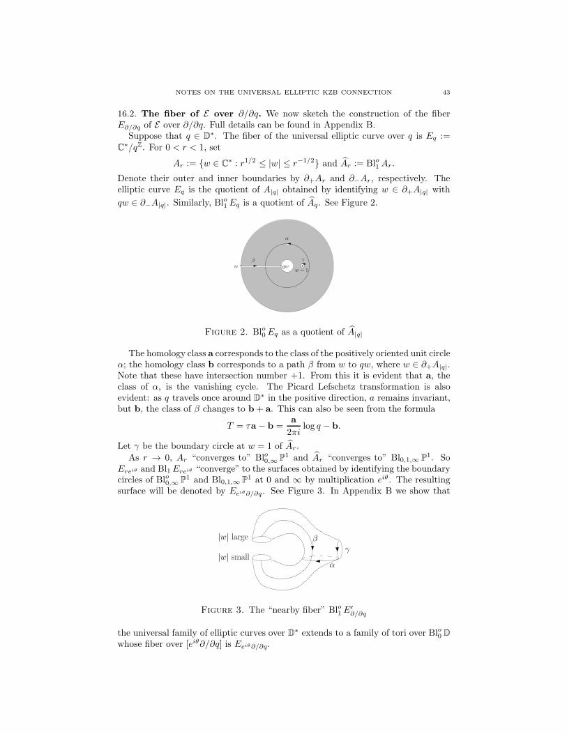
NOTES ON THE UNIVERSAL ELLIPTIC KZB CONNECTION 43
16.2. The fiber of E over ∂/∂q. We now sketch the construction of the fiberE∂/∂q of E over ∂/∂q. Full details can be found in Appendix B.
Suppose that q ∈ D∗. The fiber of the universal elliptic curve over q is Eq :=C∗/qZ. For 0 < r < 1, set
Ar := w ∈ C∗ : r1/2 ≤ |w| ≤ r−1/2 and Ar := Blo1Ar.
Denote their outer and inner boundaries by ∂+Ar and ∂−Ar, respectively. Theelliptic curve Eq is the quotient of A|q| obtained by identifying w ∈ ∂+A|q| with
qw ∈ ∂−A|q|. Similarly, Blo1Eq is a quotient of Aq. See Figure 2.
γ
α
w = 1
βw qw
Figure 2. Blo0Eq as a quotient of A|q|
The homology class a corresponds to the class of the positively oriented unit circleα; the homology class b corresponds to a path β from w to qw, where w ∈ ∂+A|q|.Note that these have intersection number +1. From this it is evident that a, theclass of α, is the vanishing cycle. The Picard Lefschetz transformation is alsoevident: as q travels once around D∗ in the positive direction, a remains invariant,but b, the class of β changes to b+ a. This can also be seen from the formula
T = τa − b =a
2πilog q − b.
Let γ be the boundary circle at w = 1 of Ar.
As r → 0, Ar “converges to” Blo0,∞ P1 and Ar “converges to” Bl0,1,∞ P1. SoEreiθ and Bl1Ereiθ “converge” to the surfaces obtained by identifying the boundarycircles of Blo0,∞ P1 and Bl0,1,∞ P1 at 0 and ∞ by multiplication eiθ. The resultingsurface will be denoted by Eeiθ∂/∂q. See Figure 3. In Appendix B we show that
γ
α
β|w| large
|w| small
Figure 3. The “nearby fiber” Blo1E′∂/∂q
the universal family of elliptic curves over D∗ extends to a family of tori over Blo0 Dwhose fiber over [eiθ∂/∂q] is Eeiθ∂/∂q.
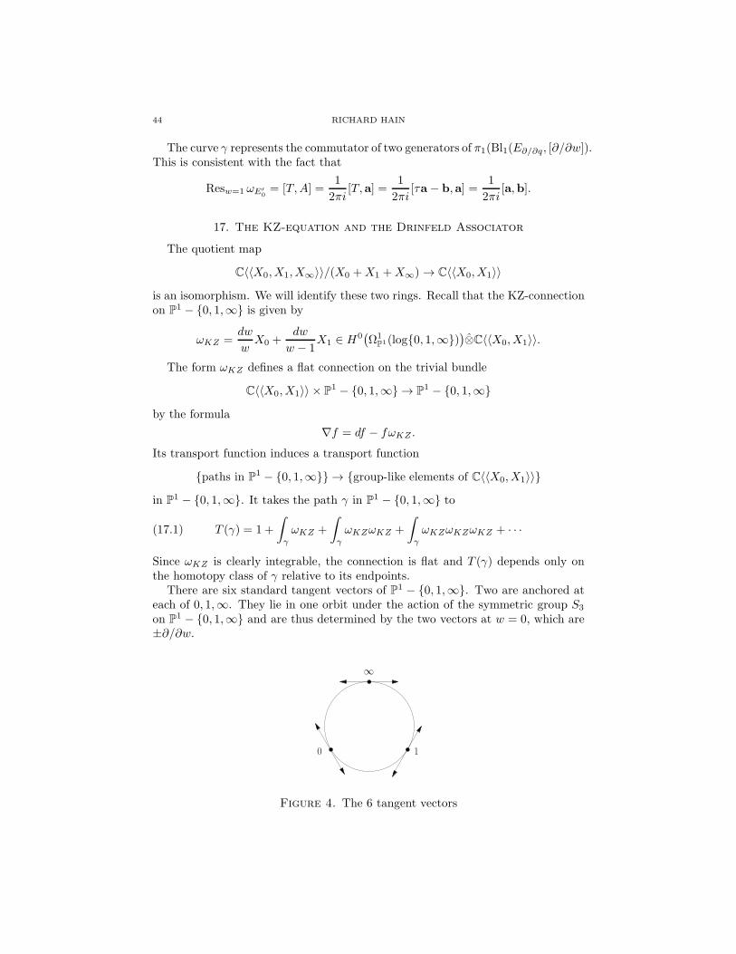
44 RICHARD HAIN
The curve γ represents the commutator of two generators of π1(Bl1(E∂/∂q, [∂/∂w]).This is consistent with the fact that
Resw=1 ωE′
0= [T,A] =
1
2πi[T, a] =
1
2πi[τa− b, a] =
1
2πi[a,b].
17. The KZ-equation and the Drinfeld Associator
The quotient map
C〈〈X0, X1, X∞〉〉/(X0 +X1 +X∞) → C〈〈X0, X1〉〉
is an isomorphism. We will identify these two rings. Recall that the KZ-connectionon P1 − 0, 1,∞ is given by
ωKZ =dw
wX0 +
dw
w − 1X1 ∈ H0
(Ω1
P1(log0, 1,∞))⊗C〈〈X0, X1〉〉.
The form ωKZ defines a flat connection on the trivial bundle
C〈〈X0, X1〉〉 × P1 − 0, 1,∞ → P1 − 0, 1,∞
by the formula
∇f = df − fωKZ .
Its transport function induces a transport function
paths in P1 − 0, 1,∞ → group-like elements of C〈〈X0, X1〉〉
in P1 − 0, 1,∞. It takes the path γ in P1 − 0, 1,∞ to
(17.1) T (γ) = 1 +
∫
γ
ωKZ +
∫
γ
ωKZωKZ +
∫
γ
ωKZωKZωKZ + · · ·
Since ωKZ is clearly integrable, the connection is flat and T (γ) depends only onthe homotopy class of γ relative to its endpoints.
There are six standard tangent vectors of P1 − 0, 1,∞. Two are anchored ateach of 0, 1,∞. They lie in one orbit under the action of the symmetric group S3
on P1 − 0, 1,∞ and are thus determined by the two vectors at w = 0, which are±∂/∂w.
1
∞
0
Figure 4. The 6 tangent vectors
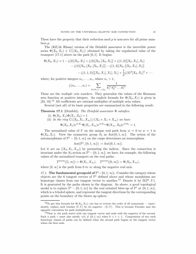
NOTES ON THE UNIVERSAL ELLIPTIC KZB CONNECTION 45
These have the property that their reduction mod p is non-zero for all prime num-bers p.
The (KZ/de Rham) version of the Drinfeld associator is the invertible powerseries Φ(X0, X1) ∈ C〈〈X0, X1〉〉 obtained by taking the regularized value of thetransport (17.1) above on the path [0, 1]. It begins:
Φ(X0, X1) = 1− ζ(2)[X0, X1] + ζ(3)[X0, [X0, X1]] + ζ(1, 2)[[X0, X1], X1]
− ζ(4)[X0, [X0, [X0, X1]]]− ζ(1, 3)[X0, [[X0, X1], X1]]
− ζ(1, 1, 2)[[[X0, X1], X1], X1] +1
2ζ(2)2[X0, X1]
2 + · · ·where, for positive integers n1, . . . , nr, where nr > 1,
ζ(n1, . . . , nr) =∑
0<k1<···<kr
1
kn1
1 kn2
2 . . . knrr.
These are the multiple zeta numbers. They generalize the values of the Riemannzeta function at positive integers. An explicit formula for Φ(X0, X1) is given in[23, 10].12 All coefficients are rational multiplies of multiple zeta values.
Several (not all) of its basic properties are summarized in the following result:
Theorem 17.1 (Drinfeld). The Drinfeld associator Φ satisfies:
(i) Φ(X0, X1)Φ(X1, X0) = 1(ii) In the ring C〈〈X0, X1, X∞〉〉/(X0 +X1 +X∞) we have
Φ(X0, X1)eiπX1Φ(X1, X∞)eiπX∞Φ(X∞, X0)e
iπX0 = 1.
The normalized value of T on the unique real path from w = 0 to w = 1 isΦ(X0, X1). View the symmetric group S3 as Aut0, 1,∞. The action of theautomorphisms of P1 − 0, 1,∞ on the cusps determines an isomorphism
Aut(P1, 0, 1,∞) → Aut0, 1,∞.Let it act on X0, X1, X∞ by permuting the indices. Since the connection isinvariant under the S3-action on P1−0, 1,∞, we have, for example, the followingvalues of the normalized transport on the real paths:
T norm([1,∞]) = Φ(X1, X∞), T norm([0,∞]) = Φ(X0, X∞),
where [0,∞] is the path from 0 to ∞ along the negative real axis.
17.1. The fundamental groupoid of P1−0, 1,∞. Consider the category whoseobjects are the 6 tangent vectors of P1 defined above and whose morphisms arehomotopy classes from one tangent vector to another.13 Denote it by Π(P1, V ).It is generated by the paths shown in the diagram. As above, a good topologicalmodel is to replace P1 − 0, 1,∞ by the real oriented blow-up of P1 at 0, 1,∞,which is a 3-holed sphere, and represent the tangent directions by the correspondingpoints on the boundary of the blown up sphere.
12To get this formula for Φ(X0,X1), one has to reverse the order of all monomials — equiv-alently, replace each bracket [U, V ] by its negative −[U, V ]. This is because Furusho uses theopposite convention for path multiplication.
13That is, the path starts with one tangent vector and ends with the negative of the second.Such a path γ must also satisfy γ(t) /∈ 0, 1,∞ when 0 < t < 1. Composition of two suchhomotopy classes of paths can be defined when the second path begins at the tangent vectorwhere the first ends.
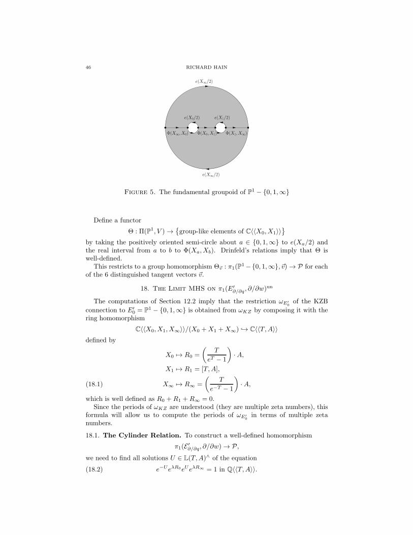
46 RICHARD HAIN
e(X∞/2)
e(X∞/2)
e(X0/2)
Φ(X0, X1)
e(X1/2)
Φ(X1, X∞)Φ(X∞, X0)
Figure 5. The fundamental groupoid of P1 − 0, 1,∞
Define a functor
Θ : Π(P1, V ) →group-like elements of C〈〈X0, X1〉〉
by taking the positively oriented semi-circle about a ∈ 0, 1,∞ to e(Xa/2) andthe real interval from a to b to Φ(Xa, Xb). Drinfeld’s relations imply that Θ iswell-defined.
This restricts to a group homomorphism Θ~v : π1(P1−0, 1,∞, ~v) → P for each
of the 6 distinguished tangent vectors ~v.
18. The Limit MHS on π1(E′∂/∂q , ∂/∂w)
un
The computations of Section 12.2 imply that the restriction ωE′
0of the KZB
connection to E′0 = P1 − 0, 1,∞ is obtained from ωKZ by composing it with the
ring homomorphism
C〈〈X0, X1, X∞〉〉/(X0 +X1 +X∞) → C〈〈T,A〉〉defined by
X0 7→ R0 =
(T
eT − 1
)·A,
X1 7→ R1 = [T,A],
X∞ 7→ R∞ =
(T
e−T − 1
)·A,(18.1)
which is well defined as R0 +R1 +R∞ = 0.Since the periods of ωKZ are understood (they are multiple zeta numbers), this
formula will allow us to compute the periods of ωE′
0in terms of multiple zeta
numbers.
18.1. The Cylinder Relation. To construct a well-defined homomorphism
π1(E ′∂/∂q, ∂/∂w) → P ,
we need to find all solutions U ∈ L(T,A)∧ of the equation
(18.2) e−UeλR0eUeλR∞ = 1 in Q〈〈T,A〉〉.
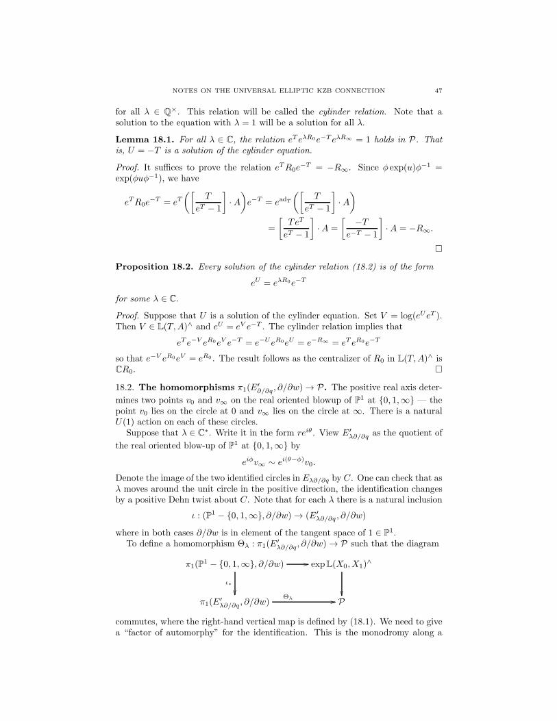
NOTES ON THE UNIVERSAL ELLIPTIC KZB CONNECTION 47
for all λ ∈ Q×. This relation will be called the cylinder relation. Note that asolution to the equation with λ = 1 will be a solution for all λ.
Lemma 18.1. For all λ ∈ C, the relation eT eλR0e−T eλR∞ = 1 holds in P. Thatis, U = −T is a solution of the cylinder equation.
Proof. It suffices to prove the relation eTR0e−T = −R∞. Since φ exp(u)φ−1 =
exp(φuφ−1), we have
eTR0e−T = eT
([T
eT − 1
]· A)e−T = eadT
([T
eT − 1
]· A)
=
[TeT
eT − 1
]·A =
[ −Te−T − 1
]·A = −R∞.
Proposition 18.2. Every solution of the cylinder relation (18.2) is of the form
eU = eλR0e−T
for some λ ∈ C.
Proof. Suppose that U is a solution of the cylinder equation. Set V = log(eUeT ).Then V ∈ L(T,A)∧ and eU = eV e−T . The cylinder relation implies that
eT e−V eR0eV e−T = e−UeR0eU = e−R∞ = eT eR0e−T
so that e−V eR0eV = eR0 . The result follows as the centralizer of R0 in L(T,A)∧ isCR0.
18.2. The homomorphisms π1(E′∂/∂q , ∂/∂w) → P. The positive real axis deter-
mines two points v0 and v∞ on the real oriented blowup of P1 at 0, 1,∞ — thepoint v0 lies on the circle at 0 and v∞ lies on the circle at ∞. There is a naturalU(1) action on each of these circles.
Suppose that λ ∈ C∗. Write it in the form reiθ. View E′λ∂/∂q as the quotient of
the real oriented blow-up of P1 at 0, 1,∞ by
eiφv∞ ∼ ei(θ−φ)v0.
Denote the image of the two identified circles in Eλ∂/∂q by C. One can check that asλ moves around the unit circle in the positive direction, the identification changesby a positive Dehn twist about C. Note that for each λ there is a natural inclusion
ι : (P1 − 0, 1,∞, ∂/∂w) → (E′λ∂/∂q , ∂/∂w)
where in both cases ∂/∂w is in element of the tangent space of 1 ∈ P1.To define a homomorphism Θλ : π1(E
′λ∂/∂q, ∂/∂w) → P such that the diagram
π1(P1 − 0, 1,∞, ∂/∂w) //
ι∗
expL(X0, X1)∧
π1(E
′λ∂/∂q , ∂/∂w)
Θλ // P
commutes, where the right-hand vertical map is defined by (18.1). We need to givea “factor of automorphy” for the identification. This is the monodromy along a
48 RICHARD HAIN
“path” from eiφv∞ to ei(θ−φ)v0. In order that Θλ be well defined, this factor ofautomorphy has to satisfy the cylinder relation.
For λ ∈ C∗, define this factor of automorphy for Θλ to be
λR0e−T := elog λR0e−T .
That is, the (inverse) monodromy in going from the tangent vector λv0 at 0 ∈ P1
to the tangent vector v∞ at ∞ is λR0e−T .
e(R∞/2)
e(R∞/2)
e(R0/2) identify outer circle
with inner circle
Φ(R∞, R0) Φ(R1, R∞)
e(R0/2)
Φ(R0, R1)
e(R1/2)
eT eT
Figure 6. The path torsor of E′∂/∂q
Give C〈〈A, T 〉〉 the Hodge, weight and relative weight filtrations defined in Sec-tion 15.
Proposition 18.3. The (complete Hopf algebra) homomorphism
Θλ : Qπ1(E′λ∂/∂q, ∂/∂w)
∧ → C〈〈T,A〉〉is an isomorphism after tensoring the source with C. This and the Hodge and weightfiltrations on C〈〈A, T 〉〉 defined in Section 15 define a MHS on Qπ1(E
′λ∂/∂q, ∂/∂w)
∧.
This is the canonical limit MHS on the fiber of the universal enveloping algebra ofPPP corresponding to the tangent vector λ∂/∂q + ∂/∂w at the identity of the nodalcubic. Its relative weight filtration is the one defined in Section 15.
Proof. Observe that Θλ induces a homomorphism H1(E′λ∂/∂q ,Z) → CT ⊕ CA. It
takes a to 2πiR0 mod I2 = 2πiA and b to log(λR0e−T ) mod I2 = logλA− T . Thehomomorphism Θλ is an isomorphism after complexifying as both its source andtarget are free and as it induces an isomorphism on I/I2.
The homomorphism Θλ defines a MHS on Qπ1(E′λ∂/∂q, ∂/∂w)
∧ by pulling back
the Hodge, weight and relative weight filtrations of C〈〈T,A〉〉. To check thatthis is the limit MHS associated to λ∂/∂q, it suffices to check that the inducedMHS on H1(Eλ∂/∂q) by Θλ agrees with the canonical limit MHS. This followsfrom the discussion above and the fact that the MHS induced on the image ofQπ1(P
1 − 0, 1,∞, ∂/∂w)∧ by Θλ is its canonical MHS, which follows from thecomputations in Section 12.2. The point being that the limit MHS on H1(Eλ∂/∂q)corresponding to λ∂/∂q determines the factor of automorphy. The computationsat the beginning of the proof imply that the MHS on H1(Eλ∂/∂q) induced by Θλ
agrees with the limit MHS that was computed in Lemma 15.3.
NOTES ON THE UNIVERSAL ELLIPTIC KZB CONNECTION 49
Part 4. The Q-de Rham Structure
Levin and Racinet [24, §5] sketch an argument to show that the elliptic KZBconnection is defined over Q. This part is an expanded exposition of a specialcase of their computation. In particular, we explicitly compute (Thm. 20.2) therestriction of the canonical extension of the universal elliptic KZB connection toM1,~1 in terms of the Q-algebraic coordinates on M1,~1. When reading [24, §5], itis important to note that that the restriction of PPP to an elliptic curve E is notalgebraically trivial. Levin and Racinet trivialize the restriction of PPP to E′. TheQ-connection they write down is on the corresponding trivial extension of PPP|E′ toE. It does not have a regular singular point at 0. However, it is important inapplications, such as those in [18], to know that the canonical extension PPP and itsconnection are defined over Q. This has been verified by Ma Luo and will appearin his Duke PhD thesis.
19. The Q-DR Structure on H over M1,~1
The first step is to compute the Q-DR structure on H and its canonical extensionH. Since M1,~1 is the moduli space of elliptic curves endowed with a non-zero
abelian differential, the Hodge bundle F 1H is trivialized by its tautological section.We show that the canonical extension of H over M1,~1 is trivial and that it and itsconnection are defined over Q. Material in this section must surely be well knownand classical (19th C).
19.1. M1,~1 as a Q-scheme. As explained in Section 1 (also see [15]), M1,~1 is the
quotient L′−1 of C×h by the action of SL2(Z) which acts with factor of automorphy
(cτ + d)−1. It is also the complement in C2 of the discriminant locus ∆ = 0, where
∆ = u3 − 27v2.
The quotient mapping C× h → C2 −∆−1(0) is
(ξ, τ) 7→(ξ4g2(τ), ξ
6g3(τ)),
where
g2(τ) = 20(2πi)4G4(τ) and g3 =7
3(2πi)6G6(τ).
The point (u, v) corresponds to the pair (Eu,v, ωu,v) where Eu,v is the elliptic curvey2 = 4x3 − ux− v and ωu,v is the abelian differential dx/y. This elliptic curve hasdiscriminant (divided by 16) equal to
∆ := u3 − 27v2 = ξ12(g32 − 27g23) = (2πiξ)12∆0,
where ∆0 = q∏
n≥1(1− qn)24 is the Ramanujan τ -function. We will view M1,~1 as
the Q-scheme SpecQ[u, v,∆−1].
19.2. Trivializing H over M1,~1. To trivialize H, we need two linearly indepen-
dent sections. The first is given by the abelian differential dx/y. The second byxdx/y, a differential of the second kind.
Set
ητ = ℘(z, τ)dz =
(1 + 2
∞∑
m=1
G2m+2(τ)
(2m)!(2πiz)2m+2
)dz
z2.
This is a differential of the second kind on Eτ .
50 RICHARD HAIN
Proposition 19.1. If γ ∈ SL2(Z), then ηγτ = (cτ + d)ητ and∫
Eτ
ωτ ητ = 2πi.
In particular, H1(Eτ ;C) = Cωτ ⊕ Cητ for all τ .
Proof. The first assertion follows easily from the definition of ητ . The second for-mula follows from a routine residue computation:
Choose a closed disk D = z : |z| ≤ R in Eτ about the origin. Let F be aholomorphic function on D satisfying F ′(z) = ℘(z). Let ϕ : Eτ → R be a smoothfunction that vanishes outside the annulus A = z : R/3 < |z| < R/2 and isidentically 1 when |z| < R/3. The 1-form
ψ := ητ − d(ϕF (z))
is smooth and closed. Since it agrees with ητ outside A, it has the same periods asητ and thus represents the same cohomology class. Since ωτ ∧ψ is supported in D,we have
〈ωτ ητ , Eτ 〉 =
∫
Eτ
ωτ ∧ ψ =
∫
D
dz ∧ ψ =
∫
∂D
zψ =
∫
∂D
z℘(z)dz = 2πi.
Remark 19.2. This implies that the exact sequence
0 → L → H → L−1 → 0
over M1,1 splits; the copy of L−1 in H is spanned locally by ητ . We will see
below that this sequence also splits over M1,1. This splitting also follows from the
vanishing of H1(M1,1,L2) as there are no modular forms of weight 2 and level 1.
Corollary 19.3. The sections ξ−1ωτ and ξητ of H over C×h are SL2(Z)-invariant.
For a lattice Λ in C, set
℘Λ(z) :=1
z2+∑
λ∈Λλ6=0
[1
(z − λ)2− 1
λ2
].
The Weierstrass ℘-function ℘(z, τ) defined in Section 8.4 is ℘Λτ (z). One checkseasily that
℘ξ−1Λ(ξ−1z) = ξ2℘Λ(z).
Multiplication by ξ−1 induces an isomorphism Eτ → C/ξ−1Λτ under which dzand ℘ξ−1Λτ
dz pull back to ξ−1ωτ and ξητ , respectively.
Proposition 19.4. If (u, v) = (ξ4g2(τ), ξ6g3(τ)
), then
(i) the mapz 7→
[℘ξ−1Λτ
(z), ℘′ξ−1Λτ
(z), 1]
from C/ξ−1Λτ to P2 induces an isomorphism C/ξ−1Λτ → Eu,v;(ii) under this isomorphism
dx/y = dz = ξ−1ωτ and xdx/y = ℘ξ−1Λτ(z)dz;
(iii) under the isomorphism Eτ → C/ξ−1Λτ → Eu,v, dx/y and xdx/y pull backto ξ−1ωτ and ξητ , respectively.
NOTES ON THE UNIVERSAL ELLIPTIC KZB CONNECTION 51
Corollary 19.5. For each (u, v) ∈ M1,~1, the elements dx/y and xdx/y of the fiber
H1(Eu,v) of H are linearly independent.
Denote these sections of H over M1,~1 by T and S, respectively. They trivializeH and determine the extension
H := OM1,~1S ⊕OM1,~1
T
of H to M1,~1.
Proposition 19.6. The connection on H with respect to this trivialization is
∇0 = d+(− 1
12
d∆
∆⊗ T +
3
2
α
∆⊗ S
) ∂
∂T+(− u
8
α
∆⊗ T +
1
12
d∆
∆⊗ S
) ∂
∂S
where α = 2udv− 3vdu and ∆ = u3− 27v2. This form is logarithmic on M1,~1 withnilpotent residue along ∆ = 0 and is therefore the canonical extension of H overM1,~1. It is defined over Q.
Sketch of Proof. We need to understand how the classes dx/y and xdx/y dependon (u, v). Each of the 1-forms
∂
∂u
(dxy
)=
1
2
xdx
y3,∂
∂v
(dxy
)=
1
2
dx
y3,∂
∂u
(xdxy
)=
1
2
x2dx
y3,∂
∂v
(xdxy
)=
1
2
xdx
y3
is a differential of the second kind on each Eu,v. So the cohomology class of eachis a linear combination of the classes of dx/y and xdx/y.
The differentials d(1/y), d(x/y) and d(x2/y), the relation 2ydy = (12x2 − u)dx,and some linear algebra give
(dxy3
xdxy3
x2dxy3
)≡ 3
∆
(dxy
xdxy
)(3v −u2/6 uv/42u −3v u2/6
)
where ≡ means congruent mod exact forms of the second kind, and thus equal incohomology.
Now
∇0
(T S
)= ∇0
(dxy
xdxy
)
=1
2
(xdxy3
x2dxy3
)du+
1
2
(dxy3
xdxy3
)dv
=3
2∆
(dxy
xdxy
)(−u2du/6 + 3vdv uvdu/4− u6dv/6−3vdu+ 2udv u2du/6− 3vdv
)
=(T S
)(− 112
d∆∆ − uα
8∆3α2∆
112
d∆∆
)
The forms α/∆ and uα/∆ are logarithmic. One can prove this directly. Alter-natively, we can use the fact [6] that a meromorphic form ϕ on C2 has logarithmicsingularities along ∆ = 0 if and only if ∆ϕ and ∆dϕ are both holomorphic along∆ = 0. This holds in our case as
∆d(α/∆) = −du ∧ dv and ∆d(uα/∆) = udu ∧ dv.Similarly, one checks that wϕ and wdϕ are holomorphic along the line at infinity,where w = 0 is a local defining equation of the line at infinity, then ϕ is logarithmicalong the line at infinity. This is easily checked when ϕ is α/∆ and uα/∆.
52 RICHARD HAIN
This implies that the sequence
0 → L → H → L−1 → 0
splits over M1,~1. The lift of L−1 in H is OM1,~1S.
19.3. Transcendental version. We re-derive the formula for the connection interms of the coordinates (ξ, τ) ∈ C × h. This will yield some formulas that areuseful in computing the algebraic version of the universal elliptic KZB connection.
As observed above, if (u, v) = (ξ4g2(τ), ξ6g3(τ)), then dx/y = ξ−1ωτ . Since T is
the class of dx/y, we have
T = ξ−1T.
Proposition 19.7. We have ητ = (2πi)2(A− 2G2(τ)T ) so that
S = ξητ = (2πi)2ξ(A− 2G2(τ)T ).
Proof. Using the notation of Example 3.4, we have
(a t
)( 18π2G2(τ)
)=(a′ t′
)((cτ + d)−1 02πic cτ + d
)(1
8π2G2(τ)
)
= (cτ + d)−1(a′ t′
)( 18π2G2(γτ)
).
From this it follows that
A− 2G2(τ)T = (cτ + d)−1(A′ − 2G2(γτ)T
′).
Consequently, A − 2G2(τ)T is a section of H that spans a copy of L−1 over h.But ητ is another such section. It follows that ητ is a holomorphic multiple ofA− 2G2(τ)T . This multiple can be determined by pairing with ωτ . Since
〈T,A− 2G2(τ)T 〉 = 〈ωτ , (2πi)−1a〉 = (2πi)−1 and 〈T, ητ 〉 =
∫
Eτ
ωτ ητ = 2πi,
it follows that
ητ = (2πi)2(A− 2G2(τ)T ).
There are several ways to prove the second assertion. One is to observe that
〈T , S〉 = 〈dxy,xdx
y〉 = 2πi = 〈T, S〉 = 〈ξ−1T, ξS〉 = 〈T , ξS〉.
We’ve already seen in Example 5.2 that the connection ∇0 on H over h withrespect to the framing A, T is given by
∇0 = d+ 2πiA∂
∂T⊗ dτ.
Proposition 19.8. With respect to the framing S and T of H over M1,~1, theconnection on H is
∇0 = d+((
4πiG2 dτ −dξ
ξ
)⊗ T +
2πi
(2πiξ)2dτ ⊗ S
) ∂
∂T
−((2πiξ)2(8πiG2
2 + 2G′2) dτ ⊗ T +
(4πiG2 dτ −
dξ
ξ
)⊗ S
) ∂
∂S
NOTES ON THE UNIVERSAL ELLIPTIC KZB CONNECTION 53
Proof. Since S/(2πi)2 = A− 2G2T ,
∇0
(T S/(2πi)2
)= ∇0
(T A
)(1 −2G2
0 1
)+(T A
)(0 −2G′2
0 0
)dτ
=(T A
)(( 0 02πi 0
)(1 −2G2
0 1
)+
(0 −2G′
2
0 0
))dτ
=(T S/(2πi)2
)(1 2G2
0 1
)(0 −2G′
2
2πi −4πiG2
)dτ
=(T S/(2πi)2
)(4πiG2 −(8πiG22 + 2G′
2)2πi −4πiG2
)dτ
Rescaling, we have
∇0
(T S
)=(T S
)( 4πiG2 −(2πi)2(8πiG22 + 2G′
2)(2πi)−1 −4πiG2
)dτ
Denote the 2× 2 matrix of 1-forms in this expression by Bdτ . Then
∇0
(T S
)= ∇0
(T S
)(ξ−1 00 ξ
)+(T S
)(−ξ−2 00 1
)dξ
=(T S
)[(ξ 00 ξ−1
)B
(ξ−1 00 ξ
)dτ +
(ξ 00 ξ−1
)(−ξ−2 00 1
)dξ
]
=(T S
)(− dξξ + 4πiG2(τ)dτ −2(2πiξ)2(4πiG2(τ)
2 +G′2(τ))dτ
2πi(2πiξ)2 dτ
dξξ − 4πiG2(τ)dτ
)
Comparing this formula with that in Proposition 19.6, we conclude:
(19.1)dξ
ξ− 4πiG2(τ)dτ =
1
12
d∆
∆and
2πi
(2πiξ)2dτ =
3α
2∆.
. Taking the quotient of the two off diagonal entries of the connection matrix, weconclude that
G4(τ) =6
5
(2G2(τ)
2 +G′2(τ)/2πi
).
This can also be verified by observing that the RHS is a modular form of weight 4and then computing value of both sides at q = 0.
20. The Q-DR Structure on PPP over M1,~1
The bundle PPP over M1,~1 is the trivial bundle whose fiber is L(S, T )∧. We willdefine a Q structure on it — that is, a Q structure on its truncations by the termsof its lower central series.
Some preliminary observations will be helpful. Since the cup product of therational differentials dx/y and xdx/y is 2πi, it is natural to multiply their Poincareduals by (2πi)−1 to obtain a Q-de Rham basis of the first homology. Motivated bythis, we define
T0 = T /2πi and S0 = S/2πi.
Since both basis elements of H are multiplied by the same constant, the formula
for the connection on H given in Proposition 19.6 remains valid when we replace S
by S0 and T by T0.
Set pQ = LQ(S0, T0)∧. Define the Q-structure on PPP to be M1,~1/Q × pQ.
54 RICHARD HAIN
Define derivations ǫǫǫ2m of pQ by
ǫǫǫ2m =
−S0
∂
∂T0
m = 0;
T 2m−10 · S0 −
∑j+k=2m−1
j>k>0(−1)j[T j
0 · S0, Tk0 · S0]
∂
∂S0
m > 0.
Lemma 20.1. For all m ≥ 0, we have (2πiξ)2m−2ǫǫǫ2m = ǫ2m in Der p.
Proof. First observe that
ǫ2m(T ) = −T 2m · A and ǫ2m(A) =∑
j>k≥0j+k=2m−1
(−1)j+1[T j · A, T k · A]
and
ǫǫǫ2m(T0) = −T 2m0 · S0 and ǫǫǫ2m(S0) =
∑
j>k≥0j+k=2m−1
(−1)j+1[T j0 · S0, T
k0 · S0].
One checks easily that, when m ≥ 1, ǫ2m(T ) = −T 2m · (A− 2G2T ) and
ǫ2m(A− 2G2T ) =∑
j>k≥0j+k=2m−1
(−1)j+1[T j · (A− 2G2T ), Tk · (A− 2G2T )].
The result follows by rescaling as T0 = T/(2πiξ) and S0 = 2πiξ(A− 2G2T ).
The connection ∇0 on H defines, and will be viewed as, a Q-rational connectionon each graded quotient of PPP .
Theorem 20.2. With respect to the framing of PPP over M1,~1 described above, theuniversal elliptic KZB-connection ∇ is given by
∇ = ∇0 +1
12
d∆
∆⊗ ǫǫǫ2 +
∑
m≥2
3
(2m− 2)!
p2m(u, v)(3vdu− 2udv)
∆⊗ ǫǫǫ2m
where ∆ = u3 − 27v2 is the discriminant and where p2m(u, v) ∈ Q[u, v] is thepolynomial characterized by (2πiξ)2mG2m(τ) = p2m(u, v). The Hodge bundles F pPPPare all defined over Q.
The polynomial p2m(u, v) is weighted homogeneous of weight 2m in u and v,where u is given weight 4 and v is given weight 6. The polynomials of weight up to
NOTES ON THE UNIVERSAL ELLIPTIC KZB CONNECTION 55
24 are:
p4(u, v) =1
20u
p6(u, v) =3
7v
p8(u, v) =3
10u2
p10(u, v) =108
11uv
p12(u, v) =756
65u3 +
16200
91v2
p14(u, v) = 1296 uv2
p16(u, v) =174636
85u4 +
1166400
17uv2
p18(u, v) =9471168
19u3v +
256608000
133v3
p20(u, v) =25147584
25u5 +
678844800
11u2v2
p22(u, v) =10671720192
23u4v +
103296384000
23uv3
p24(u, v) =73581830784
65u6 +
1410877440000
13u3v2 +
15547365504000
91v4
Proof. With respect to the framing A, T of PPP, the connection is ∇ = d+ ω′ whereω′ is the form (13.1). Since the change of frame is homogeneous, the transformedconnection is of the form ∇ = ∇0 + ω′. We just need to express ω′ in the frame
given by Lie words in S0, T0. Using the identities (19.1) and the preceding lemmawe have
ω′ = −(2G2(τ)
dq
q− dξ
ξ
)⊗ ǫ2 −
∞∑
m=2
2
(2m− 2)!G2m(τ)
dq
q⊗ ǫ2m
=1
12
d∆
∆⊗ ǫǫǫ2 −
∑
m≥2
2
(2m− 2)!(2πiξ)2mG2m(τ)
2πi
(2πiξ)2dτ ⊗ ǫǫǫ2m
=1
12
d∆
∆⊗ ǫǫǫ2 −
∑
m≥2
3
(2m− 2)!
p2m(u, v)α
∆⊗ ǫǫǫ2m
The last assertion follows from the fact that F pPPP is trivial and consists of those Liewords whose degree in T0 is ≥ −p.
21. The Q-de Rham Structure on F 2n+1H1(M1,1, S2nH)
Here we compute the Q-structure on F 2n+1H1dR(M1,1, S
2nH). The computationof the R-de Rham structure on all of H1(M1,1, S
2nH) can be found in [17, §17.2].The starting point is the isomorphisms
H0(M1,1,L2n+2) → H0(Ω1M1,1
(P )⊗ F 2nS2nH) → F 2n+1H1(M1,1, S2nH),
where P denotes the cusp q = 0. The second isomorphism takes a 1-form toits cohomology class. The first follows from the isomorphisms L ∼= F 1H and
56 RICHARD HAIN
Ω1M1,1
(P ) ∼= L2, which together induce an isomorphism
L2n+2∼= Ω1
M1,1(P )⊗ F 2nS2nH.
We now explain the Q-structure. Recall that if f is a modular form of weight2n+ 2 of SL2(Z), then
ωf := f(τ)w2ndτ ∈ E1(h)⊗ S2nH
is an SL2(Z)-invariant 1-form on h, where w := 2πiT is the section of H × h → h
that takes the value 2πiωτ at τ ∈ h and SL2(Z) acts on H = CA ⊕ CT via thefactor of automorphy (9.2).14 It gives a framing of F 1H over h. The section w
extends to a framing of F 1H over the q-disk.Denote the space of modular forms of SL2(Z) of weight m whose Fourier co-
efficients lie in the subfield F of C by Mm,F . These form a graded ring M∗,F
isomorphic to F [G4, G6].
Proposition 21.1. The Q-structure on F 2n+1H1dR(M1,1, S
2nH) is
f(q)w2n dq
q: f(q) ∈M2n+2,Q.
Proof. Embed Eτ into P2 via the mapping
z + Λτ 7→ [℘τ (z)/(2πi)2, ℘′
τ (z)/(2πi)3, 1].
The image is the plane cubic y2 = 4x3 − ux− v where
u = g2(τ)/(2πi)4 = 20G4(τ) and v = g3(τ)/(2πi)
6 =7
3G6(τ).
This curve has discriminant ∆0(τ), where ∆0 denotes the normalized cusp form ofweight 12.
With this normalization dx/y = 2πiωτ = w(τ).15 We choose it because thevalue of the section w at q = 0 is dw/w, where w is the parameter on the nodalcubic that maps 0 and ∞ to the node and 1 to the identity. (Cf. Exercise 47 in[15].)
We regard w as the section dx/y of F 1H over M1,~1 = A2Q − u3 − 27v2 = 0.
It is defined over Q. Since x has weight 2 and y weight 3, it has weight −1 underthe Gm action. If h(u, v) ∈ Q[u, v] is a polynomial of weight 2n+ 2 (where u hasweight 4 and v weight 6), then
h(u, v)
u3 − 27v2(2udv − 3vdu)w2n
is a Q-rational, Gm-invariant section of Ω1M1,~1/Q
(logD) ⊗ F 2nS2nH over M1,~1/Q,
whereD denotes the discriminant locus u3−27v2 = 0. SinceM1,1/Q = Gm\\M1,~1/Q
it descends to a section of Ω1M1,1/Q
(P )⊗ F 2nS2nH.
The identity (19.1) implies that the pullback of this form along the map h →M1,~1 defined by τ 7→ (20G4(τ), 7G6(τ)/3) is
2
3h(20G4(τ), 7G6(τ)/3
)w2n dq
q.
14Recall the definitions (11.1).15This would have been a better normalization to use in Part 4.
NOTES ON THE UNIVERSAL ELLIPTIC KZB CONNECTION 57
The result follows as M2n+2,Q is isomorphic to the polynomials in G4 and G6 withrational coefficients.
Appendix A. Vanishing of N(R0)
Here we give an elementary proof of the vanishing of Nq(R0) established inCorollary 15.2. It does not use limit mixed Hodge structures. Instead we deducethe vanishing from an identity involving Bernoulli numbers.
For non-negative integers, define polynomials
ha,b(x, y) = x2a−1y2b − x2by2a−1 + xy(x+ y)2b−1(y2a−2 − x2a−2)
= xy(y − x)(x2a−2y2b−2 + (x+ y)2b−1
∑
i+j=2a−3i,j≥0
xiyj).
in commuting indeterminants x and y. Note that
h0,n(x, y) = −∑
i+j=2n−1i,j≥0
[( 2n
i+ 1
)−(
2n
j + 1
)]xiyj
for all n ≥ 1.
Theorem A.1. For all n ≥ 1,
∑
a+b=na>0
(2a−1)
(2n
2a
)B2aB2b
B2nha,b(x, y) =
∑
i+j=2n−1i,j≥0
[( 2n
i+ 1
)−(
2n
j + 1
)]xiyj ∈ Z[x, y].
Equivalently,∑
a+b=na,b≥0
(2a− 1)B2a
(2a)!
B2b
(2b)!ha,b(x, y) = 0.
Proof. It suffices to show that
(A.1)∑
n≥0
∑
a+b=na,b≥0
(2a− 1)B2a
(2a)!
B2b
(2b)!ha,b(x, y) = 0.
Observe that∑
n≥0
∑
a+b=na,b≥0
(2a− 1)B2a
(2a)!
B2b
(2b)!u2a−1v2b =
(∑
a≥0
(2a− 1)B2a
(2a)!u2a−1
)(∑
b≥0
B2b
(2b)!v2b)
=4u
sinh2(u/2)
(v
ev − 1+v
2
)
=ueu
(eu − 1)2
(v
ev − 1+v
2
).
Denote this function of (u, v) by F (u, v). The series (A.1) is then
F (x, y)− F (y, x) +x
x+ yF (y, x+ y)− y
x+ yF (x, x + y)
which is easily to vanish by elementary algebraic manipulations.
58 RICHARD HAIN
We finish by showing that this identity is equivalent to the vanishing of Nq(R0).For this we need to relate polynomials to the free Lie algebra L(T,A). For thiswe use the Levin-Racinet calculus [24, §3.1]. Recall from Section 9.4.1 that forU, V ∈ L(A, T ),
xrys (U, V ) = [T r · U, T s · V ].
This extends linearly to an action f(x, y) (U, V ) of polynomials f(x, y) in com-muting indeterminants on ordered pairs of elements of L(T,A). When U and V areequal, one has the identity f(x, y) (U,U) = −f(y, x) (U,U), so that
2f(x, y) (U,U) = (f(x, y)− f(y, x)) (U,U).
In this case we need only consider polynomials f(x, y) satisfying f(x, y)+f(y, x) =0.
The significance of the polynomials ha,b(x, y) is given by:
Lemma A.2. For all a ≥ 0 and b ≥ 0 with a+ b > 0,
2 ǫ2a(T2b ·A) = ha,b(x, y) (A,A).
Proof. Observe that ha,b(x, y) = fa,b(x, y) − fa,b(y, x) where
fa,b(x, y) = xa(x+ y)2b−1(xa − (−y)a
)− x2a−1
((x+ y)2b − y2b
).
The result now follows from the easily verified identity
ǫ2a(T2b ·A) = fa,b(x, y) (A,A).
Theorem A.1 implies the vanishing of Nq(R0):
Nq(R0) =∑
a≥0
∑
b≥0
(2a− 1)B2a
(2a)!
B2b
(2b)!ǫ2a(T
2b · A)
=1
2
(∑
a≥0
∑
b≥0
(2a− 1)B2a
(2a)!
B2b
(2b)!ha,b(x, y)
) (A,A)
= 0.
Appendix B. The Universal Elliptic Curve over Bl+0 D
Here we justify the claim, made in Section 16, that the fiber of the universalelliptic curve over eiθ∂/∂q is obtained from the real oriented blowup of P1 at 0,∞by identifying its two boundary components with a suitable twist.
The map [0, 1) × S1 → D that takes (r, θ) to eiθ is the real oriented blowupBlo0 D → D of the disk. More generally, the map
S1 × [0, 1] → P1 defined by (φ, t) 7→ [teiφ, 1− t]
is Blo0,∞ P1 → P1. With this identification, the inclusion C∗ → Blo0,∞ P1 takes seiφ
to(φ, s/(1 + s)
).
The fiber of the universal elliptic curve over q = reiθ is the quotient of
A := (w, q) ∈ C∗ × D∗ :√|q| ≤ |w| ≤ 1/
√|q|
obtained by glueing w to qw when |w| = 1/√|q|. Write w = seiφ so that we can
identify A with
(s, φ, reiθ) ∈ R× S1 × D∗ :√r ≤ s ≤ 1/
√r.

NOTES ON THE UNIVERSAL ELLIPTIC KZB CONNECTION 59
With this identification, (1/√r, φ, reiθ) is glued to (
√r, φ+ θ, reiθ).
The function
h(r, s) =( s
1 + s−
√r
1 +√r
)( 1
1 +√r−
√r
1 +√r
)−1
induces homeomorphisms h(r, ) : [√r, 1/
√r] → [0, 1] for all r ≥ 0. It has inverse
k(r, ), where
k(r, t) =
√r − (
√r − 1)t
1 + (√r − 1)t
Define an equivalence relation on B := S1 × S1 × [0, 1)× [0, 1) by
(φ, θ, 1, r) ∼ (φ + θ, θ, 0, r).
Set B = B/∼. The map (φ, θ, t, r) → (r, θ) defines a projection π : B → Blo0 D.This is a torus bundle over Blo0 D. Its fiber Bθ over (0, θ) ∈ Blo0 D is the quotientof Blo0,∞ P1 obtained by identifying the two boundary components by a twist by
θ. The inclusion A → B defined by (s, φ, reiθ) 7→ (φ, θ, h(r, s), r) induces a mapED∗ → B that commutes with the projections to D and is a homeomorphism intoits image.
The map B → C∗ × D that takes (φ, θ, t, r) to (k(r, t)eiφ, reiθ) induces a mapB → ED such that the diagram
B //
ED
Blo0 D // D
commutes. For each θ ∈ S1, the composite C∗ → Blo0,∞ P1 → Bθ → E0 is thenatural inclusion of the smooth locus of the nodal cubic E0 given by the parameterw = seiφ. The map Blo0,∞ P1 → Bθ → E0 collapses the boundary of Blo0,∞ P1 tothe double point of E0.
References
[1] D. Bernard: On the Wess-Zumino-Witten models on the torus, Nuclear Phys. B 303 (1988),77–93.
[2] F. Brown: Mixed Tate motives over Z, Ann. of Math. 175 (2012), 949–976.[3] D. Calaque, B. Enriquez, P. Etingof: Universal KZB equations: the elliptic case, in Algebra,
arithmetic, and geometry: in honor of Yu. I. Manin. Vol. I, 165–266, Progr. Math., 269,Birkhauser, Boston, 2009, [arXiv:math/0702670]
[4] J. Carlson: Extensions of mixed Hodge structures, Journees de Geometrie Algebriqued’Angers, Juillet 1979, Sijthoff & Noordhoff, 1980, 107–127.
[5] K.-T. Chen: Iterated path integrals, Bull. Amer. Math. Soc. 83 (1977), 831–879.
[6] P. Deligne: Equations differentielles a points singuliers reguliers, Lecture Notes in Mathe-matics, Vol. 163. Springer-Verlag, 1970.
[7] P. Deligne: Theorie de Hodge, II, Inst. Hautes Etudes Sci. Publ. Math. No. 40 (1971), 5–57.[8] P. Deligne: Le groupe fondamental de la droite projective moins trois points, Galois groups
over Q (Berkeley, CA, 1987), 79–297, Math. Sci. Res. Inst. Publ., 16, Springer, 1989.[9] B. Enriquez: Elliptic associators, Selecta Math. (N.S.) 20 (2014), 491–584.
[10] H. Furusho: The multiple zeta value algebra and the stable derivation algebra, Publ. Res.Inst. Math. Sci. 39 (2003), 695–720. [arXiv:math/0011261]
[11] R. Hain: The geometry of the mixed Hodge structure on the fundamental group, AlgebraicGeometry, 1985, Proc. Symp. Pure Math. 46 (1987), 247–282.
[12] R. Hain: The de Rham homotopy theory of complex algebraic varieties, I. K-Theory 1 (1987),271–324.
60 RICHARD HAIN
[13] R. Hain: The de Rham homotopy theory of complex algebraic varieties, II. K-Theory 1 (1987),481–497.
[14] R. Hain: Relative weight filtrations on completions of mapping class groups, in Groups ofDiffeomorphisms, Advanced Studies in Pure Mathematics, vol. 52 (May, 2008), 309–368,Mathematical Society of Japan, [arXiv:0802.0814]
[15] R. Hain: Lectures on Moduli Spaces of Elliptic Curves, in Transformation Groups and ModuliSpaces of Curves, Advanced Lectures in Mathematics, edited by Lizhen Ji, S.-T. Yau no. 16(2010), 95–166, Higher Education Press, Beijing, [arXiv:0812.1803]
[16] R. Hain: Limit Structures on Unipotent Fundamental Groups of Stable Curves, in prepara-tion, 2013.
[17] R. Hain: The Hodge-de Rham Theory of Modular Groups in Recent Advances in Hodge The-ory Period Domains, Algebraic Cycles, and Arithmetic, Matt Kerr and Greogory Pearlstein,editors, 422–514. Cambridge University Press, 2016. [arXiv:1403.6443]
[18] R. Hain, M. Matsumoto: Universal mixed elliptic motives, submitted, [arXiv:1512.03975][19] R. Hain, S. Zucker: Unipotent variations of mixed Hodge structure, , Invent. Math. 88 (1987),
83–124.[20] M. Kashiwara: A study of variation of mixed Hodge structure, Publ. Res. Inst. Math. Sci. 22
(1986), no. 5, 991–1024.[21] Leopold Kronecker: Zur theorie der elliptischen Funktionen (1881). Reproduced in: Leopold
Kronecker’s Werke Volume IV, pp. 313–318. Herausgegeben auf Veranlassung der KoniglichPreussischen Akademie der Wissenschaften von K. Hensel, Chelsea, New York 1968.
[22] V. Knizhnik, A. Zamolodchikov: Current algebra and Wess–Zumino model in two dimen-
sions, Nuclear Phys. B 247 (1984), 83–103.[23] T. Le, J. Murakami: Kontsevich’s integral for the Kauffman polynomial, Nagoya Math. J.
142 (1996), 39–65.[24] A. Levin, G. Racinet: Towards multiple elliptic polylogarithms, unpublished preprint,
[arXiv:math/0703237][25] A. Pollack: Relations between derivations arising from modular forms, undergraduate thesis,
Duke University, 2009.16
[26] W. Schmid: Variation of Hodge structure: the singularities of the period mapping, Invent.Math. 22 (1973), 211–319.
[27] J.-P. Serre: A course in arithmetic, Translated from the French. Graduate Texts in Mathe-matics, No. 7. Springer-Verlag, New York-Heidelberg, 1973.
[28] J.-P. Serre: Lie algebras and Lie groups, Lectures given at Harvard University, 1964, Ben-jamin, 1965. (Second edition, Springer Verlag, 1992.)
[29] J. Silverman: Advanced Topics in the Arithmetic of Elliptic Curves, Graduate Texts inMathematics, 151. Springer-Verlag, New York, 1994.
[30] C. Peters, J. Steenbrink: Mixed Hodge structures, Ergebnisse der Mathematik und ihrerGrenzgebiete, volume 52. Springer-Verlag, 2008.
[31] J. Steenbrink, S. Zucker: Variation of mixed Hodge structure, I, Invent. Math. 80 (1985),489–542.
[32] H. Tsunogai: On some derivations of Lie algebras related to Galois representations, Publ.Res. Inst. Math. Sci. 31 (1995), 113–134.
[33] D. Zagier: Periods of modular forms and Jacobi theta functions, Invent. Math. 104 (1991),449–465.
Department of Mathematics, Duke University, Box 90320, Durham, NC 27708
E-mail address: [email protected]
16Available at: http://dukespace.lib.duke.edu/dspace/handle/10161/1281