Embed Size (px)
Citation preview

ARM LOCKING FOR LASER INTERFEROMETER SPACE ANTENNA
By
YINAN YU
A DISSERTATION PRESENTED TO THE GRADUATE SCHOOLOF THE UNIVERSITY OF FLORIDA IN PARTIAL FULFILLMENT
OF THE REQUIREMENTS FOR THE DEGREE OFDOCTOR OF PHILOSOPHY
UNIVERSITY OF FLORIDA
2011

c© 2011 Yinan Yu
2

To my parents who provided me everything in my life without any reservation
3

ACKNOWLEDGMENTS
This work would not have been possible if were not for the help from many UF
graduate students, faculty and staff. Especially I would like to express my deepest
gratitude to my PhD degree supervisor, Dr. Guido Mueller who has been everlasting
helpful and has offered all kinds of assistance, support and guidance on my research as
well as on the writing of this thesis.
I would also like to show my gratitude to my committee members, Dr. Tanner, Dr.
Whiting, Dr. Klimenko and Dr. Sarajedini, for taking their precious time to help me fulfill
my requirements for the PhD degree. I also wish to give special thanks to my current
and former lab colleagues: Vinzenz Wand, Shawn Mitryk, Dylan Sweeney and Joseph
’Pep’ Sanjuan, for their supportive assistances and productive discussions.
Finally, I would like to express my love and gratitude to my family for their support
and encouragement. Especially, I owe my passionate gratitude and love to my wife, also
academic partner, Yiliang Bao, for her heartful and considerate assistance to both my
life and career.
4
TABLE OF CONTENTS
page
ACKNOWLEDGMENTS . . . . . . . . . . . . . . . . . . . . . . . . . . . . . . . . . . 4
LIST OF TABLES . . . . . . . . . . . . . . . . . . . . . . . . . . . . . . . . . . . . . . 8
LIST OF FIGURES . . . . . . . . . . . . . . . . . . . . . . . . . . . . . . . . . . . . . 9
ABSTRACT . . . . . . . . . . . . . . . . . . . . . . . . . . . . . . . . . . . . . . . . . 13
CHAPTER
1 GRAVITATIONAL WAVE ASTRONOMY . . . . . . . . . . . . . . . . . . . . . . 15
1.1 Introduction . . . . . . . . . . . . . . . . . . . . . . . . . . . . . . . . . . . 151.2 Gravitational Radiation in General Relativity . . . . . . . . . . . . . . . . . 19
1.2.1 Propagation of Gravitational Waves . . . . . . . . . . . . . . . . . . 191.2.2 Generation of Gravitational Waves . . . . . . . . . . . . . . . . . . 211.2.3 Interaction of Gravitational Waves with Test Masses . . . . . . . . 24
1.3 Sources of Gravitational Waves . . . . . . . . . . . . . . . . . . . . . . . . 261.3.1 High Frequency Range . . . . . . . . . . . . . . . . . . . . . . . . . 271.3.2 Low Frequency Range . . . . . . . . . . . . . . . . . . . . . . . . . 28
1.3.2.1 Galactic binaries . . . . . . . . . . . . . . . . . . . . . . . 291.3.2.2 Coalescence of massive black holes . . . . . . . . . . . . 331.3.2.3 Extreme mass ratio inspirals . . . . . . . . . . . . . . . . 341.3.2.4 Cosmic gravitational background radiation . . . . . . . . . 36
1.4 Detection of Gravitational Waves . . . . . . . . . . . . . . . . . . . . . . . 371.4.1 Detection Methods . . . . . . . . . . . . . . . . . . . . . . . . . . . 381.4.2 Interferometric Detectors . . . . . . . . . . . . . . . . . . . . . . . . 41
1.4.2.1 Principle and configuration . . . . . . . . . . . . . . . . . 421.4.2.2 Noise limitations . . . . . . . . . . . . . . . . . . . . . . . 45
2 LASER INTERFEROMETER SPACE ANTENNA . . . . . . . . . . . . . . . . . 49
2.1 Overview . . . . . . . . . . . . . . . . . . . . . . . . . . . . . . . . . . . . 492.1.1 Sensitivity . . . . . . . . . . . . . . . . . . . . . . . . . . . . . . . . 502.1.2 Disturbance Reduction System . . . . . . . . . . . . . . . . . . . . 522.1.3 Interferometric Measurement System . . . . . . . . . . . . . . . . . 54
2.2 Noise Cancellation for LISA . . . . . . . . . . . . . . . . . . . . . . . . . . 592.2.1 Time Delay Interferometry . . . . . . . . . . . . . . . . . . . . . . . 59
2.2.1.1 Michelson X-combination . . . . . . . . . . . . . . . . . . 602.2.1.2 Sagnac combination . . . . . . . . . . . . . . . . . . . . . 622.2.1.3 TDI Limitations . . . . . . . . . . . . . . . . . . . . . . . . 63
2.2.2 Pre-stabilization . . . . . . . . . . . . . . . . . . . . . . . . . . . . . 642.2.2.1 Pound-Drever-Hall frequency stabilization . . . . . . . . . 652.2.2.2 Mach-Zehnder frequency stabilization . . . . . . . . . . . 67
5
2.3 Arm Locking . . . . . . . . . . . . . . . . . . . . . . . . . . . . . . . . . . 712.3.1 Architecture . . . . . . . . . . . . . . . . . . . . . . . . . . . . . . . 722.3.2 Arm Locking Sensors . . . . . . . . . . . . . . . . . . . . . . . . . . 74
2.3.2.1 Single arm locking . . . . . . . . . . . . . . . . . . . . . . 742.3.2.2 Common arm locking . . . . . . . . . . . . . . . . . . . . 792.3.2.3 Dual arm locking . . . . . . . . . . . . . . . . . . . . . . . 822.3.2.4 Sagnac arm locking . . . . . . . . . . . . . . . . . . . . . 86
2.3.3 Frequency Pulling . . . . . . . . . . . . . . . . . . . . . . . . . . . . 882.3.3.1 Doppler impact on arm locking . . . . . . . . . . . . . . . 882.3.3.2 Frequency pulling rate . . . . . . . . . . . . . . . . . . . . 902.3.3.3 Modified dual arm locking . . . . . . . . . . . . . . . . . . 94
2.3.4 Integration with Tunable Pre-stabilization References . . . . . . . . 992.3.4.1 Arm locking with Pound-Drever-Hall stabilization . . . . . 992.3.4.2 Arm locking with Mach-Zehnder stabilization . . . . . . . 1022.3.4.3 Arm locking only . . . . . . . . . . . . . . . . . . . . . . . 102
2.3.5 Arm Locking Limitations . . . . . . . . . . . . . . . . . . . . . . . . 1032.3.5.1 Limited controller gain in far-end PLL . . . . . . . . . . . 1032.3.5.2 Realistic noise sources in arm locking . . . . . . . . . . . 107
3 UNIVERSITY OF FLORIDA LISA INTERFEROMETER SIMULATOR . . . . . . 115
3.1 Optical Components . . . . . . . . . . . . . . . . . . . . . . . . . . . . . . 1153.2 Electronic Components . . . . . . . . . . . . . . . . . . . . . . . . . . . . 117
3.2.1 Digital Signal Processing Hardware . . . . . . . . . . . . . . . . . . 1173.2.2 Phasemeter . . . . . . . . . . . . . . . . . . . . . . . . . . . . . . . 118
3.2.2.1 Design . . . . . . . . . . . . . . . . . . . . . . . . . . . . 1193.2.2.2 Performance . . . . . . . . . . . . . . . . . . . . . . . . . 121
3.2.3 Electronic Phase Delay . . . . . . . . . . . . . . . . . . . . . . . . 122
4 EXPERIMENTAL VERIFICATION OF SINGLE ARM LOCKING . . . . . . . . . 125
4.1 Motivation . . . . . . . . . . . . . . . . . . . . . . . . . . . . . . . . . . . . 1254.2 Preliminary Test With Numerical Control Oscillator (NCO) Tracking . . . . 127
4.2.1 Experimental Setup . . . . . . . . . . . . . . . . . . . . . . . . . . 1274.2.2 Digital Filter Design . . . . . . . . . . . . . . . . . . . . . . . . . . . 1304.2.3 Measurement Results . . . . . . . . . . . . . . . . . . . . . . . . . 1324.2.4 Noise Analysis . . . . . . . . . . . . . . . . . . . . . . . . . . . . . 136
4.3 Single Arm Locking Integrated with a Tunable Reference . . . . . . . . . . 1384.3.1 Heterodyne Phase-locked Loop . . . . . . . . . . . . . . . . . . . . 139
4.3.1.1 Experimental setup . . . . . . . . . . . . . . . . . . . . . 1394.3.1.2 Closed-loop dynamics . . . . . . . . . . . . . . . . . . . . 1414.3.1.3 Results and analysis . . . . . . . . . . . . . . . . . . . . . 143
4.3.2 Piezoelectric Transducer (PZT) Actuated Cavity . . . . . . . . . . . 1464.3.2.1 Characterization of the PZT cavity . . . . . . . . . . . . . 1464.3.2.2 Experimental setup . . . . . . . . . . . . . . . . . . . . . 1484.3.2.3 Results and analysis . . . . . . . . . . . . . . . . . . . . . 150
6

4.3.3 Electro-optic Modulator (EOM) Sideband Locking . . . . . . . . . . 152
5 EXPERIMENTAL VERIFICATION OF DUAL/MODIFIED DUAL ARM LOCKING 154
5.1 Common Arm Locking . . . . . . . . . . . . . . . . . . . . . . . . . . . . . 1545.1.1 Common Arm Locking Sensor . . . . . . . . . . . . . . . . . . . . . 1545.1.2 Preliminary Test with Numerical Control Oscillator (NCO) Tracking 156
5.2 Dual Arm Locking . . . . . . . . . . . . . . . . . . . . . . . . . . . . . . . 1595.2.1 Dual Arm Locking Sensor . . . . . . . . . . . . . . . . . . . . . . . 1595.2.2 Preliminary Test with NCO Tracking . . . . . . . . . . . . . . . . . . 1615.2.3 Integration with Pre-stabilized Laser . . . . . . . . . . . . . . . . . 166
5.3 Modified Dual Arm Locking . . . . . . . . . . . . . . . . . . . . . . . . . . 1685.3.1 Modified Dual Arm Locking Sensor . . . . . . . . . . . . . . . . . . 1685.3.2 Preliminary Test with NCO Tracking . . . . . . . . . . . . . . . . . . 1705.3.3 Integration with Pre-stabilized Laser . . . . . . . . . . . . . . . . . 172
5.4 Arm locking Integrated With Far-end Phase-locking . . . . . . . . . . . . . 1735.4.1 Transponder Noise Floor - Time Domain Simulation . . . . . . . . . 1755.4.2 Experimental Verification - Simple Model . . . . . . . . . . . . . . . 1775.4.3 Experimental Verification - Full Model . . . . . . . . . . . . . . . . . 179
6 DOPPLER FREQUENCY ERROR IN ARM LOCKING . . . . . . . . . . . . . . 187
6.1 Doppler Frequency Error in LISA . . . . . . . . . . . . . . . . . . . . . . . 1876.2 Investigation of Frequency Pulling on UFLIS . . . . . . . . . . . . . . . . . 189
6.2.1 Generation of Doppler Frequency Errors . . . . . . . . . . . . . . . 1906.2.2 Frequency Pulling in Single Arm Locking . . . . . . . . . . . . . . . 1916.2.3 Frequency Pulling in Dual and Modified Dual Arm Locking . . . . . 193
6.2.3.1 Time-domain simulations with AC-coupled controller . . . 1936.2.3.2 Experiments with modified dual arm locking sensor . . . 196
7 CONCLUSION AND OUTLOOK . . . . . . . . . . . . . . . . . . . . . . . . . . 202
7.1 Control System of Arm Locking . . . . . . . . . . . . . . . . . . . . . . . . 2027.2 Noise Limitations . . . . . . . . . . . . . . . . . . . . . . . . . . . . . . . . 2037.3 Doppler-induced Frequency Pulling . . . . . . . . . . . . . . . . . . . . . . 2047.4 Outlook . . . . . . . . . . . . . . . . . . . . . . . . . . . . . . . . . . . . . 205
REFERENCES . . . . . . . . . . . . . . . . . . . . . . . . . . . . . . . . . . . . . . . 207
BIOGRAPHICAL SKETCH . . . . . . . . . . . . . . . . . . . . . . . . . . . . . . . . 214
7

LIST OF TABLES
Table page
2-1 Parameters of the noise analysis for arm locking . . . . . . . . . . . . . . . . . 110
5-1 Parameters in time-domain arm locking simulations with transponder noise . . 175
6-1 Parameters in AC-coupled dual arm locking simulations with Doppler errors . . 194
6-2 Parameters of the AC-coupled filter used in simulations . . . . . . . . . . . . . 194
8

LIST OF FIGURES
Figure page
1-1 Inspiral of a white dwarf binary system . . . . . . . . . . . . . . . . . . . . . . . 30
1-2 Artist’s illustration of an EMRI . . . . . . . . . . . . . . . . . . . . . . . . . . . . 35
1-3 Schematic of a basic Michelson interferometer . . . . . . . . . . . . . . . . . . 41
1-4 Strain sensitivities of LIGO S6 . . . . . . . . . . . . . . . . . . . . . . . . . . . 47
2-1 Heliocentric orbit of the LISA constellation . . . . . . . . . . . . . . . . . . . . . 50
2-2 LISA sensitivity curve . . . . . . . . . . . . . . . . . . . . . . . . . . . . . . . . 51
2-3 Interferometric Measurement System of LISA . . . . . . . . . . . . . . . . . . . 55
2-4 Interferometers on the optical bench of LISA . . . . . . . . . . . . . . . . . . . 56
2-5 Michelson X-combination and Sagnac combination . . . . . . . . . . . . . . . . 61
2-6 Pound-Drever-Hall frequency stabilization . . . . . . . . . . . . . . . . . . . . . 65
2-7 Mach-Zehnder frequency stabilization for LISA . . . . . . . . . . . . . . . . . . 68
2-8 Arm locking architecture in the LISA constellation . . . . . . . . . . . . . . . . . 72
2-9 Magnitude and phase responses of the single arm locking sensor . . . . . . . 75
2-10 Instability of single arm locking when using a 1/s controller . . . . . . . . . . . 76
2-11 Typical values of ∆ which indicates the noise suppression . . . . . . . . . . . . 78
2-12 Example of the closed-loop transfer function of single arm locking . . . . . . . 79
2-13 Time domain simulation to demonstrate initial transients in single arm locking . 80
2-14 Transfer function of the common arm locking sensor . . . . . . . . . . . . . . . 81
2-15 Transfer functions of the differential arm and the integrated differential arm . . 82
2-16 Transfer function of the linear combination H(s) . . . . . . . . . . . . . . . . . . 84
2-17 Transfer function of the dual arm locking sensor . . . . . . . . . . . . . . . . . . 85
2-18 Transfer function of the Sagnac-based dual arm locking sensor . . . . . . . . . 87
2-19 Generic single arm locking loop with a Doppler frequency error . . . . . . . . . 90
2-20 Generic dual arm locking loop with Doppler frequency errors . . . . . . . . . . 92
2-21 Magnitude and phase responses of the modified dual arm locking sensor . . . 95
9

2-22 Magnitude and phase responses of the dual and common components . . . . 96
2-23 Generic modified dual arm locking loop with Doppler frequency errors . . . . . 97
2-24 Magnitude responses of H+(s) and H−(s) for modified dual arm locking . . . . 98
2-25 PZT actuation cavity as a tunable reference for arm locking . . . . . . . . . . . 100
2-26 Sideband cavity lock as a tunable reference for arm locking . . . . . . . . . . . 101
2-27 Heterodyne phase-locking as a tunable reference for arm locking . . . . . . . . 101
2-28 Arm locking with the phase-locked laser at the far spacecraft . . . . . . . . . . 103
2-29 Arm locking with various noise sources . . . . . . . . . . . . . . . . . . . . . . 108
2-30 Noise floors in common arm locking . . . . . . . . . . . . . . . . . . . . . . . . 111
2-31 Noise floors in dual arm locking . . . . . . . . . . . . . . . . . . . . . . . . . . . 112
2-32 Noise floors in modified dual arm locking . . . . . . . . . . . . . . . . . . . . . 113
3-1 Frequency noise of the cavity stabilized laser . . . . . . . . . . . . . . . . . . . 116
3-2 Implementation of the phasemeter on a Pentek board . . . . . . . . . . . . . . 119
3-3 Phasemeter performance measured with split-and-subtracted VCO signals . . 121
3-4 Transfer function and noise floor of the EPD unit tested with 1 s delay . . . . . . 124
4-1 Experimental setup of single arm locking using an NCO to track the input noise 128
4-2 Single arm locking with NCO tracking - Laplace domain . . . . . . . . . . . . . 129
4-3 Magnitude response of controller for single arm locking . . . . . . . . . . . . . 131
4-4 Magnitude response of the 1/√s filter . . . . . . . . . . . . . . . . . . . . . . . 132
4-5 Noise spectra of the single arm locking test at high frequencies . . . . . . . . . 132
4-6 Time series of the single arm locking test at high frequencies . . . . . . . . . . 133
4-7 Noise spectra of the single arm locking test at low frequencies . . . . . . . . . 134
4-8 Time series of the single arm locking test at low frequencies . . . . . . . . . . . 134
4-9 Single arm locking with NCO tracking - Laplace domain with noise sources . . 135
4-10 Comparison with a 30-bit digitization noise floor . . . . . . . . . . . . . . . . . . 137
4-11 Comparison of frequency drift rate between a 30-bit filter and a 32-bit filter . . . 138
4-12 Experimental setup of single arm locking using a phase-locked laser . . . . . . 140
10

4-13 Single arm locking with heterodyne PLL - Laplace domain . . . . . . . . . . . . 141
4-14 Noise spectra of single arm locking with heterodyne PLL . . . . . . . . . . . . . 144
4-15 Single arm locking with heterodyne PLL - Laplace domain with noise sources . 145
4-16 Experimental setup of single arm locking using a PZT actuated cavity . . . . . 148
4-17 Single arm locking with a PZT cavity - Laplace domain . . . . . . . . . . . . . . 149
4-18 Noise spectra of single arm locking with a PZT actuated cavity . . . . . . . . . 151
4-19 Single arm locking with a PZT cavity - Laplace domain with noise sources . . . 152
5-1 Design of the common arm locking sensor and the sensor transfer function . . 155
5-2 Experimental setup of common arm locking using NCO tracking . . . . . . . . 156
5-3 Noise spectra of common arm locking test with NCO tracking . . . . . . . . . . 157
5-4 Common arm locking with NCO tracking in the Laplace domain . . . . . . . . . 158
5-5 Lock acquisition process in common arm locking . . . . . . . . . . . . . . . . . 159
5-6 Implementation diagram of the dual arm locking sensor . . . . . . . . . . . . . 160
5-7 Magnitude responses of the dual arm locking sensor . . . . . . . . . . . . . . . 161
5-8 Preliminary experimental setup of dual arm locking with NCO tracking . . . . . 162
5-9 Noise spectra of dual arm locking with NCO tracking . . . . . . . . . . . . . . . 163
5-10 Noise spectra of 48-bit dual arm locking with NCO tracking . . . . . . . . . . . 164
5-11 Lock acquisition process in dual arm locking . . . . . . . . . . . . . . . . . . . 165
5-12 Experimental setup of dual arm locking using a phase-locked laser . . . . . . . 166
5-13 Noise spectra of dual arm locking with heterodyne PLL . . . . . . . . . . . . . 167
5-14 Implementation diagram of the modified dual arm locking sensor . . . . . . . . 168
5-15 Magnitude responses of the modified dual arm locking sensor . . . . . . . . . . 169
5-16 Experimental setup of modified dual arm locking with NCO tracking . . . . . . 170
5-17 Noise spectra of the modified dual arm locking test with NCO tracking . . . . . 171
5-18 Magnitude responses of H+(s) and H−(s) used in the experiment . . . . . . . . 172
5-19 Experimental setup of modified dual arm locking using a phase-locked laser . . 173
5-20 Noise spectra of dual arm locking with heterodyne PLL . . . . . . . . . . . . . 174
11

5-21 Time domain simulation of modified dual arm locking with transponder noise . 177
5-22 Experimental setup of dual arm locking with FG signal as the transponder noise 178
5-23 Noise spectra of dual arm locking with FG signal as the transponder noise . . . 180
5-24 Experimental setup of modified dual arm locking with far-end PLL . . . . . . . 181
5-25 Closed-loop dynamics of modified dual arm locking with far-end PLL . . . . . . 182
5-26 Noise spectra of the transponder noise observed in modified dual arm locking . 185
5-27 Noise spectra of the stabilized laser frequency and the transponder noise floor 186
6-1 Experimental setup of AC-coupled single arm locking with Doppler error . . . . 192
6-2 Measurement results of AC-coupled single arm locking with Doppler error . . . 192
6-3 Performance of dual arm locking with an AC-coupled controller . . . . . . . . . 195
6-4 Experimental setup of dual/modified dual arm locking with Doppler errors . . . 197
6-5 Frequency pulling of dual/modified dual arm locking with Doppler errors . . . . 197
6-6 Performance of modified dual arm locking in the presence of Doppler errors . . 198
6-7 Linear drift in the laser frequency stabilized by modified dual arm locking . . . 199
6-8 Frequency pulling in lock acquisition due to a step function in Doppler errors . 200
12

Abstract of Dissertation Presented to the Graduate Schoolof the University of Florida in Partial Fulfillment of theRequirements for the Degree of Doctor of Philosophy
ARM LOCKING FOR LASER INTERFEROMETER SPACE ANTENNA
By
Yinan Yu
May 2011
Chair: Guido MuellerMajor: Physics
The Laser Interferometer Space Antenna (LISA) is a collaborative National
Aeronautics and Space Administration (NASA)/European Space Agency (ESA) space
mission to detect gravitational waves in the frequency region of 3 × 10⁻⁵ Hz to 1 Hz by
means of laser interferometry. It will be the first space-based interferometric gravitational
wave detector to be launched in 2020s. LISA will consist of three identical spacecraft
arranged in a quasi-equilateral triangular constellation with 5 Gm on each side. Each
spacecraft houses two drag-free proof masses that follow the geodesic motion. The
Interferometric Measurement System (IMS) of LISA monitors changes in the proper
distance between two proof masses on each respective spacecraft.
Laser frequency stabilization is one of the most significant and difficult issues for
the IMS of LISA. Arm locking as a proposed frequency stabilization technique, transfers
the stability of the long arm lengths to the laser frequency. The arm locking sensor
synthesizes an adequately filtered linear combination of the inter-spacecraft phase
measurements to estimate the laser frequency noise, which can be used to control the
laser frequency. Due to the large propagation delay during the light transmission, the
arm locking controller needs to be carefully designed to retain enough phase margin.
A potential problem for arm locking is that the Doppler shift of the return beam will
cause a constant pulling in the master laser frequency if unaccounted for in the phase
measurement. Until now all the benchtop experiments on arm locking verified only the
13

basic single arm locking configuration with unrealistic short delay time and without any
Doppler estimation error at the phasemeter. At the University of Florida we developed
the hardware-based University of Florida LISA Interferometer Simulator (UFLIS) to study
and verify laser frequency noise reduction and suppression techniques under realistic
LISA-like conditions. These conditions include the variable Doppler shifts between the
spacecraft, LISA-like signal travel times, far-end heterodyne phase-locking, realistic
laser frequency and timing noise. In this dissertation we will systematically introduce
the cutting edge of experimental studies of arm locking under these realistic conditions.
We have built an analog/digital hybrid system to demonstrate the control system of
various arm locking schemes and their incorporation with pre-stabilization subsystems.
We measured the noise suppression in our experiments as well as the frequency
pulling in the presence of Doppler frequency error. With the achievement of meeting
the requirement, our pioneering work have sufficiently demonstrated the validity and
feasibility of arm locking under LISA-like conditions.
14

CHAPTER 1GRAVITATIONAL WAVE ASTRONOMY
1.1 Introduction
Since the dawn of human civilization, the curiosity to the universe has always
been a primary motivation for human to pursue science. Einstein once said, “The most
incomprehensible thing about the world is that it is comprehensible.” The observational
astronomy is undoubtedly a first step in human’s historical attempts to understand the
universe, thanks to electromagnetic waves that allowed Aristotle to observe celestial
constellations by naked eyes and allowed Galileo to observe Jupiter and orbiting moons
by optical telescopes. Starting from the 19th century, the universe observable to human
has been substantially expanded from visible light to currently the full spectrum of
electromagnetic waves. A variety of ground-based and space-based observatories,
covering from radio to Gamma ray, have been developed to study the evolution of stars
and galaxies, as well as the origin of the universe.
In addition to the magnificent achievements electromagnetic observations have
already obtained, another different observation method started to gradually grow in
the second half of the 20th century. Gravity, as the dominant force in the universe,
results in gravitational waves generated from accelerated objects, which is predicted
by Einstein’s General Theory of Relativity. In this theory, gravitational waves are
oscillations of spacetime geometry propagating with the speed of light [1]. Einstein
never thought gravitational waves could possibly be detected due to their extremely
weak interactions with matters. Nevertheless, Joseph Weber started to build the very
first gravitational wave detectors using resonant masses in 1960s [2]. Also during this
period, general relativity began to demonstrate its power in the research of astrophysics
and cosmology. Relativistic gravity, as well as gravitational radiations, were found to
play an important role in various astronomical systems. The most famous example of
gravitational radiations is the 13-year observation to the binary pulsar PSR1913+16
15

[3, 4], which first indirectly verified the existence of gravitational waves, as well as the
validity of general relativity in strong gravitational fields. The success of PSR1913+16
indicates that like electromagnetic waves, gravitational waves can also be used as
an observation method to study the universe, which is known as gravitational wave
astronomy.
Actually, gravitational wave astronomy will reveal abundant information about
astronomical systems that could not be achieved by traditional electromagnetic wave
astronomy [5]. For example, the gravitational radiation from black hole coalescence
provides the only possible direct observation method to study black hole physics.
The electromagnetic radiation from black holes (known as Hawking radiation), if any,
would be impossible to detect for current technology. Also due to the weak interaction
with matters, gravitational waves are hardly attenuated or scattered ever since they
are generated. This indicates that they could carry information about some exotic
phenomena that electromagnetic detections cannot reach, such as the interior of
supernova explosions or physics of the very early universe.
Although the prospect of gravitational wave astronomy is exciting, the detection of
gravitational waves still remains to be a challenge for current technology due to their
extremely weak interactions with masses. For example, the typical upper limit of the
gravitational wave strain generated by the coalescence of stellar mass black holes is
no more than 10−23 when arrive at the Earth. The manifestation of gravitational wave
strains is an oscillating change in the relative distance between test masses. Based
on this principle, laser interferometers can be naturally used to construct gravitational
wave detectors via precise interferometry. The ground-based Laser Interferometer
Gravitational Wave Observatory (LIGO) is based on an equal-armed Michelson
interferometer with arm lengths of 4 km [6]. Nevertheless, the required displacement
sensitivity is still on the order of ∼ 10−19 m Hz−1/2. To reach the required sensitivity,
16

various techniques have been developed for LIGO and other ground-based detectors to
enhance their detection sensitivity and suppress random noises.
LIGO and other ground-based detectors are expected to detect gravitational
waves at frequencies higher than ∼ 30 Hz. For frequencies below ∼ 30 Hz, the
seismic noise from ground vibrations starts to dominate the sensitivity curve rapidly and
becomes a limitation for current ground-based detectors. The detection of gravitational
waves at lower frequencies requires either a completely different detection method
or an absolute isolation from seismic noise by placing the detector in space. Laser
Interferometer Space Antenna (LISA) is a proposed large-scaled laser interferometer
on the heliocentric orbit in order to detect gravitational waves at frequencies from
3 × 10⁻⁵ Hz to 1 Hz [7, 8]. LISA consists of three spacecraft forming a near-equilateral
triangle with each side length 5 × 10⁹ m. Since the arm length is far longer than all
ground-based detectors, the length change due to gravitational wave strains will become
more significant, which provides LISA a sensitivity of 10−20 Hz−1/2 at 3 mHz. With this
sensitivity, LISA will be able to detect low-frequency gravitational waves emitted from
coalescences of massive black holes (MBH) out to redshift z ∼ 20 [9, 10]. Other primary
gravitational wave sources LISA will detect include extreme mass ratio inspirals (EMRI)
where the dynamics of a test mass captured in Kerr geometry can be experimentally
studied, resolved and unresolved Galactic compact binaries, even gravitational relics of
Big Bang known as the stochastic background and maybe cosmic strings predicted
in some versions of the string theory. In summary, LISA will perform a series of
new scientific measurements to various gravitational wave sources in the universe
with multiple goals, including relevant astrophysical research in such as binaries and
galaxies, tests of general relativity in strong gravitational fields, as well as discoveries of
new physics and cosmology.
Like the Michelson interferometer used in ground-based detectors, LISA will also
measure the change in distance between two free-falling proof masses. However,
17

the configuration and operation of LISA are quite different from a standard Michelson
interferometer in a number of ways. As LISA consists of three spacecraft and each
of them orbits the sun independently, the arm length between two proof masses is a
time-variable quantity, which cannot be made identical to each other even in principle.
Time Delay Interferometry (TDI) as a post-processing technique synthesizes equal
arm interferometry to extract gravitational wave signals [11, 12]. Nevertheless, the
random fluctuations in the laser frequency cannot be suppressed adequately by TDI
with limited precision of the arm length knowledge. To overcome this problem, the
pre-stabilization of the laser frequency is essential. In addition to common methods
such as Pound-Drever-Hall technique used for the laser stabilization in ground-based
detectors, the architecture of LISA inherently provides a unique frequency stabilization
technique known as arm locking. Since the LISA arm length is a very stable reference
in the LISA frequency band, arm locking takes it as a frequency reference to stabilize
the laser frequency via the synthesization of an adequately filtered linear combination
of the interferometry signals. The main subject of this dissertation is about arm locking,
including the analytical performance [13], numerical simulations in the time domain and
especially the experimental verification in laboratory [14, 15].
This dissertation is divided into seven chapters. The remaining part of Chapter
1 introduces the theory of gravitational radiation, gravitational wave sources and
detections. In this part I put emphasis on the gravitational wave sources for LISA.
Chapter 2 covers the overview of LISA, including the scientific requirements and
payload, where the technique of arm locking is the main subject to be focused on.
Chapter 3 to Chapter 6 discuss the experimental verifications of arm locking on the
hardware simulator of LISA interferometry developed at the University of Florida. The
final part, Chapter 7, gives the conclusions and outlook on arm locking and LISA
interferometry.
18

1.2 Gravitational Radiation in General Relativity
1.2.1 Propagation of Gravitational Waves
Gravitational radiation is one of the most fundamental phenomena predicted by
Einstein’s General Theory of Relativity. The propagation of gravitational waves in
spacetime can be described as an approximate solution of linearized Einstein field
equations in the presence of a weak gravitational field. 1
The Einstein field equations can be written as
Rµν −1
2gµνR =
8πG
c4Tµν. (1–1)
We assume the gravitational field is weak enough such that the metric gµν can be
decomposed into the flat Minkowski metric plus a small linear perturbation, i.e.,
gµν = ηµν + hµν, |hµν | ≪ 1. (1–2)
This approximation is known as the theory of linearized gravity where only the first
order of the perturbation hµν is taken into account. In this theory the overall spacetime
metric gµν can be described as a perturbation tensor field hµν propagating within the flat
Minkowski spacetime. This tensor field is symmetric and Lorentz invariant.
To solve the Einstein field equations using this approximation, we calculate the
Riemann curvature tensor
Rµνρσ =1
2(∂ν∂ρhµσ + ∂µ∂σhνρ − ∂µ∂ρhνσ − ∂ν∂σhµρ). (1–3)
We define the trace of the perturbation as h = ηµνhµν and the trace-reverse metric
perturbation as hµν = hµν − 12ηµνh. Based on the Riemann tensor calculated in Eq.1–3,
1 The theoretical introduction of general relativity and gravitational waves in thischapter is mainly adapted from Ref. [16] by Misner et al.and Ref. [17] by Maggiore.
19
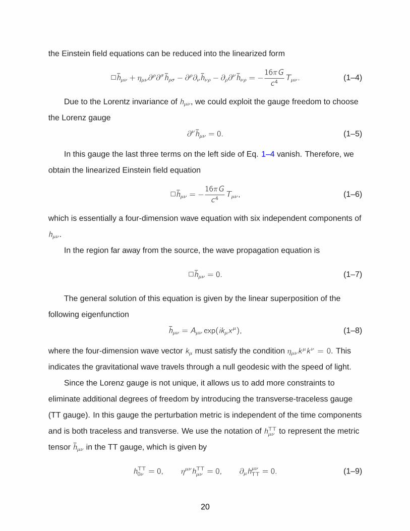
the Einstein field equations can be reduced into the linearized form
2hµν + ηµν∂ρ∂σhρσ − ∂ρ∂ν hνρ − ∂ρ∂
ν hνρ = −16πGc4Tµν. (1–4)
Due to the Lorentz invariance of hµν , we could exploit the gauge freedom to choose
the Lorenz gauge
∂ν hµν = 0. (1–5)
In this gauge the last three terms on the left side of Eq. 1–4 vanish. Therefore, we
obtain the linearized Einstein field equation
2hµν = −16πGc4Tµν, (1–6)
which is essentially a four-dimension wave equation with six independent components of
hµν .
In the region far away from the source, the wave propagation equation is
2hµν = 0. (1–7)
The general solution of this equation is given by the linear superposition of the
following eigenfunction
hµν = Aµν exp(ikµxµ), (1–8)
where the four-dimension wave vector kµ must satisfy the condition ηµνkµkν = 0. This
indicates the gravitational wave travels through a null geodesic with the speed of light.
Since the Lorenz gauge is not unique, it allows us to add more constraints to
eliminate additional degrees of freedom by introducing the transverse-traceless gauge
(TT gauge). In this gauge the perturbation metric is independent of the time components
and is both traceless and transverse. We use the notation of hTTµν to represent the metric
tensor hµν in the TT gauge, which is given by
hTT0ν = 0, ηµνhTTµν = 0, ∂µhµνTT = 0. (1–9)
20

Under the constraints of both the Lorenz gauge and the TT gauge, the metric tensor
has only two independent components, corresponding to two orthogonal modes of linear
polarization of gravitational waves. If we assume the gravitational wave travels in the z
direction, the metric tensor can be completely characterized by the form
hTTµν (t, z) =
h+ h× 0
h× −h+ 0
0 0 0
cos[ω(t − z/c)], (1–10)
where the notations of h+ and h× are known as the plus and the cross polarizations
of gravitational waves, respectively. Eq. 1–10 can also be written in the form of a
spacetime interval:
ds2 = −cdt2 + dz2 + [1 + h+ cos(ω(t − z/c))]dx2
+ [1− h+ cos(ω(t − z/c))]dy 2 + 2h× cos(ω(t − z/c))dxdy . (1–11)
1.2.2 Generation of Gravitational Waves
In the region near the radiation source, the energy-momentum tensor Tµν does not
vanish. By solving the matter-coupled Einstein equation, we could obtain the relation
between the motion of the source and generation of gravitational waves. Generally, an
inhomogeneous wave equation such as
2hµν = −16πGc4Tµν (1–12)
can be solved using the retarded Green’s function, which is also used for similar
problems in electromagnetism. We consider the radiation from a four-dimension point
source δ(4)(x − x ′) and then the Green’s function G(x − x ′) is the solution for the wave
equation: 2xG(x − x ′) = δ(4)(x − x ′), where 2x represents the d’Alembertian operator
with derivatives respective to the field point x .
21
The retarded Green’s function can be expressed as
G(x − x ′) = − 1
4π|x− x′|δ(x0ret − x ′
0
), (1–13)
where x ′0= ct ′, x0ret = ctret and tret ≡ t − |x−x′|
cis called the retarded time.
Thus the solution for Eq. 1–12 is given by the integration
hµν(t, x) = −16πGc4
∫G(x − x ′)Tµν(x
′) d4x ′
=4G
c4
∫1
|x− x′|Tµν
(t − |x− x′|
c, x′
)d3x ′. (1–14)
If the radiation source Tµν is non-relativistic, which means the typical velocities
inside the source are significantly smaller than the speed of light, in the far field
approximation we have
hµν(t, x) ≈4G
c41
r
∫Tµν
(t − rc, x′
)d3x ′, (1–15)
where r = |x− x′| is the spatial distance.
With the Lorenz gauge condition and the conservation law of the energy-momentum
tensor ∂µT µν = 0, the formula can be further reduced into
hµν(t, x) =2G
c41
r
d2Iµν
dt2(t − r
c), (1–16)
where
Iµν =
∫x ′µx
′νT00(t, x′) d3x ′ (1–17)
is defined as the quadrupole moment tensor of the energy density of the source. If the
source is a perfect fluid with a rest frame energy density ρ, the quadrupole moment
tensor is simply equivalent to the moment of inertia of the source. Eq. 1–16 is known
as the quadrupole formula, which indicates that the gravitational wave strain generated
from a non-relativistic source is proportional to the second derivative of the quadrupole
moment tensor. In contrast, the leading term in an electromagnetic radiation is a
time-changing dipole moment.
22

It is easy to show that for a binary system that consists of two stars with mass
M and orbital radius R, the orbital frequency is given by forb = 12π
√GM4R3
. From the
quadrupole formula, one can deduce that the gravitational wave frequency of this binary
system is twice of the orbital frequency, i.e., fGW = 2forb.
The luminosity (i.e., the total power) of the gravitational quadrupole radiation is
given by
LGW =G
5c5
⟨d3-I µνdt3
d3-I µνdt3
⟩
=G
5c5
⟨d3Iµν
dt3d3Iµν
dt3− 13
(d3I
dt3
)2⟩, (1–18)
where -I µν = Iµν − 13δµν I =
∫(x ′µx
′ν − 1
3δµνr
2)T 00(t, x′) d3x ′ is known as the reduced
quadrupole moment, which is the counterpart of the reduced quadrupole moment in
electromagnetism. The angle brackets represent an average over several characteristic
wavelengths of the source.
Now we will estimate how much the power the gravitational radiation has. First,
the third time derivative of the reduced quadrupole moment has the same order of
magnitude to the quantity MR2/T 3, where M is the accelerated mass, R is the size of
the radiation system and T is the time for the mass to move from one side to the other.
For a binary system T can be considered as the orbital period. On the other hand, the
quantity MR2/T 3 can be written as
MR2
T 3=M(R/T )2
T∼ Ekinetic
T∼ Linternal, (1–19)
where Ekinetic is the translational kinetic energy of the accelerated mass when moving
from one side to the other and Linternal is the internal luminosity or the power inside the
system flowing from one side to the other.
23

Therefore, a rough estimation of Eq. 1–18 is given by the square of the internal
luminosity:
LGW ∼ Gc5L2internal. (1–20)
From this relation one can further deduce how long the gravitational radiation will
need to exhaust the total energy of the system. We will explain the binary system as an
example in Section 1.3.2.
1.2.3 Interaction of Gravitational Waves with Test Masses
The motion of a test mass in a curved spacetime is described by the geodesic
equation:d2xµ
dτ 2+ Γµνρ
dxν
dτ
dxρ
dτ= 0. (1–21)
We consider two nearby geodesics, which are parametrized by xµ(τ) and xµ(τ) +
ξµ(τ) respectively. If we take the difference between their geodesic equations and
expand it to the first order since |ξµ| is very small, it yields
d2ξµ
dτ 2+ 2Γµνρ
dxν
dτ
dξρ
dτ+ ξσ∂σΓ
µνρ
dxν
dτ
dxρ
dτ= 0. (1–22)
This equation can be written in a simpler form if we introduce the covariant
derivative DVµ
Dτ≡ dVµ
dτ+ ΓµνρV
ν dxρ
dτ, which is known as the geodesic deviation equation:
D2ξµ
Dτ 2= −Rµ
νρσξρdx
ν
dτ
dxσ
dτ. (1–23)
Therefore, the geodesic deviation equation describes a tidal gravitational force
applying on nearby geodesics. To further derive how the test mass behaves in the
presence of the tidal force, we will need to choose a reference frame.
In the TT gauge gravitational waves can be represented as simple as in Eq. 1–10.
We consider two test masses with a coordinate separation ξ i and if they are at rest at
τ = 0, we have dx i/dτ = 0 and dx0/dτ = c . Therefore, Eq. 1–22 is reduced to
d2ξ i
dτ 2= −
(2cΓi0ρ
dξρ
dτ+ c2ξσ∂σΓi00
), (1–24)
24

Moreover, in the TT gauge the Christoffel symbol
Γi00 =1
2(2∂0h0i − ∂ih00) (1–25)
also vanishes since h00 and h0i equal zero in the TT gauge. The only non-vanishing term
is Γi0j =12∂0hij and then the equation is further simplified into
d2ξ i
dτ 2= −hij
dξ i
dτ. (1–26)
Therefore, if the two test masses do not have an initial relative velocity dξi
dτ, then
we also have d2ξi
dτ2= 0 and their coordinate distance always remains the same. In other
words, in the TT gauge the position of test masses does not change due to gravitational
waves. This conclusion does not imply that the interaction of gravitational waves with
test masses is zero; instead, what gravitational waves change is the proper distance
between test masses as demonstrated in Eq. 1–11. If we assume that the coordinates
of the two test masses are given by (0, 0, 0, 0) and (0,L, 0, 0), from Eq. 1–11 the proper
distance is then given by
s = L(1 + h+ cos(ωt))1/2 ≈ L(1 + 1
2h+ cos(ωt)). (1–27)
Due to the invariance of the TT gauge, gravitational wave detectors require a more
convenient reference frame to measure the position change of test masses. Such
a reference frame known as the proper detector frame requires the test mass to be
drag-free (at least in certain directions) and its relevant coordinates will be changed by
gravitational waves. In this frame the geodesic deviation equation yields
ξ i =1
2¨hTTij ξj . (1–28)
where the second order derivative is with respect to the coordinate time rather than the
proper time.
25
Starting from Eq. 1–28, we consider a gravitational wave propagating along the z
axis and the test masses are located in the x-y plane. At z = 0, the + polarization can
be written as
hTTab = h+ sinωt
1 0
0 −1
, a, b = 1, 2. (1–29)
Substitute Eq. 1–28 with Eq. 1–29 and we obtain the coordinate changes on x and
y directions:
δx = −h+2(x0 + δx)ω2 sinωt,
δy =h+
2(y0 + δy)ω2 sinωt. (1–30)
Ignore the negligible δx , δy terms on the right side and integrate twice over time:
δx =h+
2x0 sinωt,
δy = −h+2y0 sinωt. (1–31)
Similar approach can be performed to evaluate the coordinate changes due to the ×
polarization:
δx =h×2y0 sinωt,
δy =h×2x0 sinωt. (1–32)
Eq. 1–31 and Eq. 1–32 describes how gravitational waves displace test masses
transversely with respect to their propagation direction. This kind of tidal distortions is
the measurement principle behind all resonant and interferometric gravitational wave
detectors.
1.3 Sources of Gravitational Waves
In this section we have a review on typical astrophysical gravitational wave
sources classified by their radiation frequencies. The frequency range for observable
26
gravitational wave sources starts from ∼ 10 kHz and extends downward by roughly 22
orders of magnitude [18].
In Section 1.2.2 we already mentioned that the frequency of gravitational waves
emitted from a binary system is twice of the orbital frequency. In general cases, the
gravitational wave frequency of a certain source is of the same order to the natural
frequency of the system, which is given by
f0 =
√ρG
4π, (1–33)
where ρ is the mean density of the mass-energy in the source. It can be simply
estimated by ρ = 3M4πR3
, where M is the mass and R is the radius. Therefore, a
gravitational wave source with a higher mean density will radiates at a higher frequency.
For a neutron star with a 1.4M⊙ mass and a 10 km radius, the gravitational wave
frequency is close to 2 kHz. For a white dwarf with a 0.5M⊙ mass and a 104 km radius,
the gravitational wave frequency is close to 3 mHz, which is in the LISA science band.
For black holes, since the Schwarzschild radius of a black hole is related to the mass:
R = 2GM/c2, the natural frequency is inversely proportional to the black hole mass. For
a 10M⊙ stellar mass black hole the frequency is close to 1 kHz, while for a 2.5 × 10⁶M⊙
massive black hole the frequency is as low as 4 mHz.
1.3.1 High Frequency Range
The gravitational wave sources in this high frequency range will be detected by
ground-based interferometric detectors as well as resonant bars. These sources include
the coalescence of neutron star and stellar mass black holes, gravitational collapse of
supernovae, spinning pulsars and stochastic radiation background from the Big Bang.
We will introduce the inspiral binaries and the stochastic background in the next section
(Low frequency range) and this section only involves sources that are exclusive to the
high frequency range.
27

One particularly interesting high-frequency source is spinning pulsars. To radiate
gravitational waves, the mass-energy distribution of the pulsar must be asymmetric
otherwise the quadrupole moment is time-independent. The mechanism to produce this
asymmetry could be a “lump”, where the asymmetry is static relative to the neutron star,
or a “wave”, where the asymmetry is in motion. The former cases can possibly be seen
in spheroid-shaped neutron stars [19], neutron stars with a misalignment of the magnetic
field with the rotation axis or neutron stars with accretions. Since the contribution to
gravitational radiations is completely from the asymmetric portion, the gravitational
wave frequency of a pulsar is also twice of the spinning frequency. Since the spinning
frequency of a pulsar is ultra stable, the gravitational wave signal will be seen in a very
narrow frequency bin. Unlike inspiral binaries, the gravitational radiation of a pulsar is
probably not the primary mechanism to cause it to spin down [18].
In addition, the core collapse of a supernova that forms a new neutron star
or black hole is also likely to be an important source in the high frequency range.
The rotational core collapse of a supernova is asymmetric, which was already
confirmed by observations to the supernova SN 1987A [20]. This asymmetry may
be associated with a transient and non-periodic burst signal. However, the waveform
and amplitude predictions of burst signals are very difficult to model analytically and so
far relies entirely on numerical simulations. It is yet not clear what fraction of the total
mass-energy will be released in the form of gravitational radiation. The current best
estimation yields an upper limit of 10−6 [18], which makes the gravitational bursts in the
Virgo cluster undetectable. In comparison, the rate of core collapse supernovae in our
Galaxy is estimated to be one per a few decades and the corresponding burst signal
should be detectable for current detectors.
1.3.2 Low Frequency Range
In this section we will focus on the gravitational wave sources in the LISA science
band, including galactic binaries, coalescence of massive black holes, extreme mass
28

ratio inspirals and cosmic gravitational radiation background. 2 The science objective
of LISA is to detect and study the gravitational radiations from these unprecedentedly
observed sources. Based on the detection results, LISA will comprehensively reveal
more astrophysical information on binaries, black holes, galaxy structures, etc. LISA will
also precisely test the validity of general relativity in very strong gravitational fields like
the vicinity of a Kerr black hole. Finally, LISA will probe new physics and cosmology by
tracing gravitational waves from the very early universe.
1.3.2.1 Galactic binaries
The inspiral of compact binary systems is the best understood gravitational wave
source and so far the only observationally confirmed source. In Einstein’s theory,
gravitational radiations damp the energy from the orbital motion and cause the orbit to
gradually shrink. This phenomenon has already been confirmed in the observation
to the binary pulsar PSR1913+16 by Hulse and Taylor since 1974 [3, 4]. As the
two neutron stars inspiral closer, the orbital frequency continues to increase, which
generates a chirp signal in the form of gravitational radiations. In PSR1913+16 one
member is a radio pulsar, which provides a very accurate clock for orbital period
measurements. On the other hand, both the quadrupole amplitude and the orbital decay
rate only depend on the masses of the binary system (see below). The orbital decay
rate therefore can be directly predicted by general relativity, given that the required
parameters are already obtained by other observations. By comparing the theoretical
and the measured orbital decay rate, the prediction of general relativity is successfully
verified with an observational error less than 1%.
Here we will derive how a binary orbit evolves in the presence of gravitational
radiation braking. Suppose we have two stars of masses m1 and m2 on an elliptical orbit
2 For a comprehensive review of gravitational wave sources in the LISA science band,see Ref. [21].
29

Figure 1-1. Artist’s illustration of a white dwarf binary system in the inspiral phase,courtesy of NASA.
with an angular velocity ω and the semi-major axis of the elliptical orbit is a. Then the
Kepler’s law yields
ω2a3 = (m1 +m2)G = MG . (1–34)
From the virial theorem, the kinetic energy of the binary system is given by
Ekinetic = −12Epotential =
G
2
m1m2
a. (1–35)
Based on Eq. 1–20, the luminosity of the gravitational radiation is proportional to the
square of the orbiting power, which is given by the product of the kinetic energy and the
angular velocity:
LGW ∼ Gc5L2internal ∼
G
c5
(ωG
2
m1m2
a
)2
∼ G4µ2M3
4c5a5, (1–36)
where µ = m1m2/M is the reduced mass.
If we follow an exact calculation, the result is given by
LGW =32G 4µ2M3
5c5a5f (e), (1–37)
30

where f (e) is a correction function due to the eccentricity. For a circular orbit with e = 0,
we have f (e) = 1.
For binary systems, the decay rate of the total energy is equal to the gravitational
radiation power, i.e.,dEtotal
dt= −LGW, (1–38)
where the total energy Etotal just equals to the negative of the kinetic energy.
We are interested in the decay rate of the orbital period dT/dt. Based on the
Kepler’s law, the period is associated to the kinetic energy via the relation T = const ·
(−Ekinetic)−3/2. By taking derivatives on each side we have
T
T= −32
Ekinetic
Ekinetic. (1–39)
Substitute with Eq. 1–38 and we have
T
T= −96
5
G 3µM2
c5a4f (e), (1–40)
which can be further written as
T
T= −96
5
G 5/3µM2/3
c5
(T
2π
)−8/3f (e). (1–41)
If we assume f (e) = 1, the solution of this differential equation is
T (t) =
(T8/30 − 8
3kt
)3/8, (1–42)
where T0 is the period at t = 0 and the constant k is given by
k =96
5c5(2π)8/3(Gµ3/5M2/5)5/3. (1–43)
Eq. 1–42 describes how fast the orbital period of a binary system decreases over
time due to gravitational radiations, which completely depends on the constant k .
Eq. 1–43 indicates that the speed of orbit shrinking only depends on the combination
µ3/5M2/5 from the binary masses. This combination is known as the chirp mass of the
31

binary system:
Mchirp = µ3/5M2/5 = (m1m2)3/5(m1 +m2)
−1/5. (1–44)
In other words, the chirp mass of the binary system determines how fast the
frequency of the chirp signal sweeps the spectrum. By observing the time-varying
frequency of the gravitational radiation, one can directly deduce the chirp mass of the
binary system.
Since most stars in the universe have a stellar mass and also are binaries, white
dwarf binaries are numerous in the Galaxy, much more than neutron star or black hole
binaries. Although the gravitational radiation from white dwarfs is relatively weak, the
close distance in our Galaxy ensures a high SNR ∼ 100 at relatively high frequencies
(> 1 mHz). These two conditions make the white dwarf binaries the guaranteed
sources for LISA. LISA should be capable of detecting thousands of them individually
and measuring their physical parameters such as distance, orbital period and spatial
orientation precisely [22]. In particular, a number of resolved white dwarf binaries with
a short orbital period (a few minutes) are expected to be detected soon after LISA is
engaged. LISA can use them as instrument verification sources by measuring and
comparing their distances and physical parameters [23]. In addition, LISA is also
expected to detect neutron star and stellar mass black hole binaries that are at in-band
low frequencies [24, 25].
On the other hand, the population of white dwarf binaries in the Galaxy is very
large (∼ 107) at frequencies below a 1 mHz [26]. These galactic binaries form a
confusion-dominated foreground, whereas a diffuse background is generated from
extragalactic binaries. Consequently, only the brightest and closest sources among the
confusion foreground can be particularly resolved by LISA. Nevertheless, this foreground
is still of interest for LISA measurements since it represents statistical information such
as the total number and geometrical distribution of the galactic binaries in this frequency
region.
32

1.3.2.2 Coalescence of massive black holes
Massive black holes are black holes of mass 105M⊙ to 109M⊙. Abundant evidences
indicate that almost every galaxy has a massive black hole in its center. They are
thought to be the “engine” to power up active galactic nuclei (AGN) and quasars [27].
Due to the gigantic mass, the frequency of gravitational radiations from coalescences
of massive black holes is much lower yet the amplitude is much more significant than
stellar mass black holes. The gravitational radiation from coalescences of massive black
holes is the strongest signal that LISA is expected to detect. The detection range can
reach as far as z ∼ 20 and the signal is even well above the noise amplitude with a high
SNR of 102 to 103. Also compared to stars, the dimension of galaxies is not insignificant
relative to the distance between each other, which makes the galaxy merger rate
actually rather high. Therefore, LISA should be able to detect the mergers of massive
black holes with a decent detection rate, approximately 1 per year at redshift z < 1 [28].
This estimation does not take into account the formation of galaxies via mergers of small
protogalaxies of mass up to 106M⊙. If these protogalaxies also contain a seed black
hole of mass 104M⊙ in their center, the merger rate for LISA may be as high as one
thousand per year.
Same as stellar mass black hole binaries, the coalescence of massive black hole
binaries can be divided into three phases: inspiral, merger and ringdown [29, 30]. The
inspiral and ringdown phase can be analytically modeled by the post-Newtonian (PN)
approximation and the perturbation theory, while a full description of the merger phase
requires numerical relativity [31]. During the inspiral phase the two black holes are
separated far from each other (R ≫ 4M) and spiral together with an initial velocity
v/c ∼ 0.05, which can be considered as an adiabatic evolution. Like galactic binaries,
LISA will be able to measure the physical parameters during the inspiral phase with
very high accuracy. During the emission of gravitational radiations, the two black holes
approach each other and the orbit eventually decays to the Innermost Stable Circular
33

Orbit (ISCO). In Schwarzschild geometry, the ISCO is located at RISCO = 6GM/c2, where
M = m1 +m2 is the total mass of the black hole binary.
When their distance becomes shorter than rISCO, two black holes plunge into
each other and their horizons start to merge into one, forming a distorted black hole.
During the merger phase the velocity of black holes can reach v/c ∼ 0.5 and the
post-Newtonian approximation breaks down. However, numerical relativity could exploit
the precise parameters obtained in the inspiral phase to predict the merger waveform
[32]. The merge of two black holes radiates a transient yet extremely energetic burst
signal, which features a very high SNR of thousands for mergers of 106M⊙ at z = 1.
At the end of the merger, the merged black hole starts to settle down from an
excited state. During this ringdown phase, the excited black hole radiates gravitational
waves in a style of damped oscillations. Eventually it will be stabilized into a stable Kerr
black hole, which is entirely characterized by the mass and spin angular momentum,
as required by the no-hair theorem. This process can be modeled using a linear
perturbation theory in Kerr spacetime. The ringdown waveform is given by the
superposition of a whole set of quasi-normal modes solved by the perturbation theory
[33]. By detecting the damped oscillations from the black hole in the ringdown phase,
LISA should be able to confirm if a massive black hole is actually in the galaxy center
and identify a Kerr black hole from its mass and spin angular momentum. Also, it is a
test of general relativity in a extremely strong gravitational field.
1.3.2.3 Extreme mass ratio inspirals
A particularly interesting class of source for LISA is known as extreme mass ratio
inspirals (EMRIs), in which a small compact object is captured by a massive black
hole and inspirals into it [34]. The small compact object in a EMRI can be a white
dwarf, neutron star or stellar mass black hole, while LISA will probably detect EMRIs
with stellar mass black holes mostly. This is mainly because black holes tend to be
concentrated to the galactic center due to dynamic mass segregation. Also compared to
34

Figure 1-2. Artist’s illustration of an EMRI in the center of a galaxy, courtesy of NASA.
EMRIs with white dwarfs or neutron stars, EMRIs with black holes will radiate observable
signals with a higher SNR. The formation mechanism of EMRIs is conjectured to be
two-body scattering, where a compact object sufficiently close to the galactic center
happens to be captured by the massive black hole and subsequently driven onto a
highly eccentric orbit (close to 1). As the compact object orbits the massive black hole,
gravitational radiation shrinks the orbit and decreases the orbital eccentricity, causing
the compact object to spiral in until the it is finally disrupted by the tidal force [35].
In the last years of inspiral before plunge, EMRI will be radiating continuously at
frequencies to which LISA is sensitive (∼ 3 mHz). Due to the extreme mass ratio,
the inspiral process is very slow, which makes an individual waveform observable for
∼ 105 cycles/yr [36]. Most abundant EMRIs for LISA detections are believed to consist
of a stellar mass black hole of ∼ 10M⊙ and a massive black hole of ∼ 106M⊙. LISA
is capable of detecting such events within z ∼ 1 and the nearest events in one year
may be no further away than z = 0.1. Provided the generation mechanism of two-body
scattering, the rate of EMRI formations in our Galaxy is approximately one per 4 million
years [37]. This generation rate corresponds to a conservative LISA detection rate of 50
35

per year yet with a large uncertainty due to the weak constraints on stellar populations
near galactic nuclei [38].
EMRIs provide an excellent signal to study the Kerr spacetime. Although early
EMRI radiations due to highly eccentric orbits are widely discrete in time and thereby
unresolvable for LISA, the radiation in the last years of inspiral is believed to faithfully
encode the information of the surrounding Kerr spacetime. The motion of the compact
object in the Kerr spacetime is geodesic in a short time scale, while for a longer time
scale the parameters of the geodesic motion will adiabatically precess due to the orbital
circularization. Also, the orbital plane is expected to have Lense-Thirring precession
ascribed to the black hole spin. By detecting these intriguing features, LISA should be
able to precisely measure the mass and spin angular momentum of the central black
hole [39]. If the observed gravitational wave signals are uniquely determined by the
measured mass and spin, as required by the no-hair theorem, one can further confirm
that the central massive object is a Kerr black hole. If they do not satisfy the no-hair
theorem, one can deduce that the central massive object is something else like a boson
star [40].
Although the theoretical model of EMRI is seemingly simple due to the extreme
mass ratio, the high orbital eccentricity caused by two-body scattering complicates
the waveform. So far, the EMRI waveforms still cannot be completely calculated from
the perturbation theory. The most common method exploits numerical solutions of
Einstein equations in the perturbation theory, known as Teukolsky formalism [41]. In
this formalism the field equation describes the perturbative fields in a Kerr metric and a
whole set of Teukolsky-based (TB) waveforms have been solved extensively.
1.3.2.4 Cosmic gravitational background radiation
Analogous to the cosmic microwave background (CMB), a stochastic background
of gravitational waves with a frequency range of 10−18 Hz to high frequencies beyond
∼ 10 kHz was produced in the early universe. The primordial gravitational waves
36

decoupled from matter at the Planck time of ∼ 10−43 s and traveled through the universe
almost without any attenuation or scattering. Therefore, the detection of the cosmic
gravitational wave background might be an exclusive way to directly probe the physics
in the very early universe. The stochastic background of gravitational waves is usually
described in their energy density, which can be expressed as a fraction Ωgw of the critical
energy density of the universe. Although the specific value of the energy density is
still uncertain, an upper limit has been determined by the constraints from Big Bang
nucleosynthesis (BBN), as well as observations to the anisotropy of the CMB and the
period of pulsar signals. The observation of COBE to the CMB indicates an upper limit
of Ωgw < 10−13 at 10−18 Hz [42].
The stochastic background of gravitational waves may have been generated from
the amplification of quantum fluctuations during inflation, which transferred energy into
the fluctuations and converted them into gravitational waves. The conventional inflation
theory predicts a flat spectrum of Ωgw that is independent of frequencies, which makes
the energy density of the inflation-induced background far below the sensitivity of LIGO,
LISA (∼ 10−10 at 1 mHz) or pulsar timing. However, the actual energy density might
still be much higher than the conventional expectation in some variations of the inflation
theory [43, 44]. Besides inflation, there are other two mechanisms that may produce
stochastic gravitational background: the first-order electroweak phase transition [45, 46]
and cosmic strings [47]. Theoretically, these two mechanisms may produce gravitational
waves with an observable energy density for LISA in its science band.
1.4 Detection of Gravitational Waves
Theories and observations have indicated that the gravitational wave sources in our
universe are numerous and full of information, yet we still lack a reliable tool to measure
them. Without direct detections of gravitational radiation from astrophysical systems,
gravitational wave astronomy cannot be considered a branch of observational astronomy
in the real sense. Starting from 1960s, researchers have been endeavoring in order to
37

enhance gravitational wave astronomy from “the beginning of knowledge” to “the stage
of science”. In this section we will have a review on various detection techniques that
have been developed or at least proposed.
1.4.1 Detection Methods
The pioneering detection method, known as the resonant mass detector or the “bar”
detector, was proposed and built by Joseph Weber in the early 1960s [2]. A typical bar
detector consists of a cylinder made of aluminum with a length of L ∼ 3 m and a radius
of R ∼ 30 cm. The sensitivity of the bar detector is attributed to the sharp resonance of
the cylinder. Bar detectors typically have a resonant frequency of f0 ∼ 500 Hz to 1.5 kHz.
If the frequency of the gravitational wave is very close (within a few Hz) to the resonant
frequency of the bar detector, it will be absorbed and excite mechanical vibrations in the
cylinder. In theory, a short gravitational wave burst with a strain h will drive a mechanical
vibration with an amplitude δL ∼ hL. For a decent strain amplitude of 10−21, the vibration
will have an amplitude of ∼ 10−21 m. To readout such a tiny oscillation, a series of
mechanical oscillation amplifier and resonant transducers are implemented to amplify
the oscillation and convert it into a measurable electric signal.
The sensitivity of a well-suspended and isolated bar detector is primarily limited
by three intrinsic sources of noise [5, 48]. The first noise source is the thermal noise of
the atoms in the cylinder. Compared with Weber’s original design that was operated at
room temperature, current detectors are cooled to cryogenic temperatures (∼ 100 mK)
to reduce the thermal noise. Nevertheless, the thermal noise at this temperature is still
too high such that the oscillator is required to have a high mechanical quality factor
Q ∼ 106 to further suppress the thermal noise. The second noise source is introduced
by the readout chains, such as the electronic noise from the amplifier and transducer,
as well as the reverse effect of the transducer that converts the electric signal into
an mechanical force applying on the cylinder, known as the back-action noise. The
readout noise limits the detector bandwidth within a very narrow range (∼ 1 Hz) around
38

the resonant frequency. The third kind of noise is a quantum effect coming from the
zero-point vibrations.
In addition to bar detectors, electromagnetic waves can also be used to precisely
measure the change in the coordinate distance between test masses. In an electromagnetic
detection the gravitational wave modulates the propagation time of the electromagnetic
wave by disturbing the motion of test masses. So far, developed detection methods
based on electromagnetic detections fall into three categories:
• Spacecraft ranging
• Pulsar timing
• Interferometry
In the first method, the test masses are Earth and a free-falling spacecraft in
geodesic motions. During the detection a communication signal is emitted from
the transmitter on Earth and travels to the spacecraft. The spacecraft is usually a
scientific probe in a Jupiter or Saturn mission, in order to get a long transmission time
(∼ 2 − 4 × 10³ s). At the spacecraft the signal will be coherently transponded back and
returned to Earth. By monitoring the outgoing and returning time of the communication
signal, one can deduce the effect of gravitational waves on the signal propagation.
Similar measurements under the same principle can be performed by tracking the
Doppler shift frequency added onto the communication signal [49], since gravitational
waves will induce relative motions between test masses. The fractional change in the
communication signal frequency is given by
∆ν
ν=1
2cos 2φ[(1−cos θ)h(t)−2 cos θh(t−l/c−l cos θ/c)−(1+cos θ)h(t−2l/c)], (1–45)
where l is the Earth-spacecraft distance at angle θ to the propagation direction on the
z-axis. φ is the angle between the principle polarization vector of the gravitational wave
and the projection of the spacecraft position on the transverse plane. This equation
indicates that an impulse in h(t) will appear at three different times in the Doppler shift
39

frequency, known as the three-pulse response. It should be noted that time delays or
Doppler shifts caused by other classical and relativistic effects (e.g., orbital motions,
Shapiro time delay, etc.) need to be modeled and subtracted out from the measurement
data.
Pulsar timing exploits the extreme regularity of pulsar signals as a timing reference
to monitor the time of arrival (TOA) to the Earth. The timing data from pulsars can be
analyzed to search for low-frequency gravitational waves [50], especially the upper limit
of the energy density of the cosmic stochastic background [51]. The fractional change in
the pulse frequency due to gravitational waves is given by
∆ν
ν=1
2cos 2φ(1− cos θ)[h(t)− h(t − l/c − l cos θ/c)], (1–46)
where l is the Earth-pulsar distance at angle θ to the propagation direction on the z-axis.
φ is the angle between the principle polarization vector of the gravitational wave and the
projection of the pulsar position on the transverse plane. In comparison to Eq. 1–45,
an impulse in h(t) only appears at two different times in the frequency change, thereby
known as the two-pulse response due to the one-way transmission from the pulsar to
the Earth.
In data analysis, the actual TOA of radio pulses is compared with a theoretical
model based on Eq. 1–46, which yields a timing residual δt. In theory, pulsar timing is
capable of detecting gravitational waves on the order of magnitude h(f ) ∼ δt · f , where
f is the gravitational wave frequency. This gives a strain sensitivity of 10−15 − 10−16
at 10−9 Hz. In practical measurements, the data of timing residuals will be correlated
between different pulsars with a number of N to enhance the detection sensitivity, which
yields h(f ) ∼ δt · f /√N. In addition to influences of the intrinsic timing jitter and local
instrument noises, the radio pulses also encounter a series of interstellar medium (ISM)
effects during the propagation, such as dispersion, scattering, scintillation and refraction,
which require additional measurements and analysis to correct them.
40
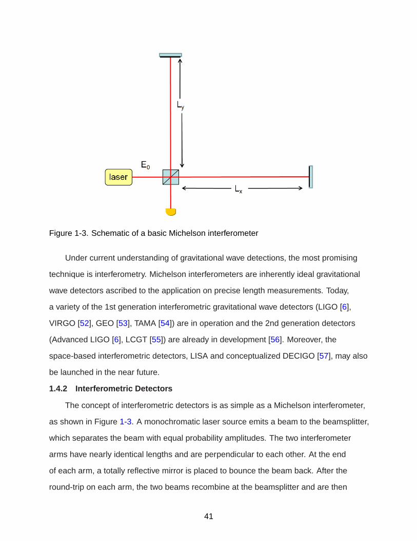
Figure 1-3. Schematic of a basic Michelson interferometer
Under current understanding of gravitational wave detections, the most promising
technique is interferometry. Michelson interferometers are inherently ideal gravitational
wave detectors ascribed to the application on precise length measurements. Today,
a variety of the 1st generation interferometric gravitational wave detectors (LIGO [6],
VIRGO [52], GEO [53], TAMA [54]) are in operation and the 2nd generation detectors
(Advanced LIGO [6], LCGT [55]) are already in development [56]. Moreover, the
space-based interferometric detectors, LISA and conceptualized DECIGO [57], may also
be launched in the near future.
1.4.2 Interferometric Detectors
The concept of interferometric detectors is as simple as a Michelson interferometer,
as shown in Figure 1-3. A monochromatic laser source emits a beam to the beamsplitter,
which separates the beam with equal probability amplitudes. The two interferometer
arms have nearly identical lengths and are perpendicular to each other. At the end
of each arm, a totally reflective mirror is placed to bounce the beam back. After the
round-trip on each arm, the two beams recombine at the beamsplitter and are then
41

received by the photodetector. The mirrors in a ground-based interferometer are not
free-falling due to the suspension to balance the gravity, but they still can be used as test
masses since we are only concerned with the horizontal plane. If gravitational waves
modulate the arm lengths into Lx and Ly , the laser power received at the photodetector
is proportional to
|EPD|2 = E 20 sin2[kL(Ly − Lx)], (1–47)
where E0 is the magnitude of the input electric field and kL is the wavenumber of
the laser. Here we take into account the π phase shift in the reflected beam at the
beamsplitter.
1.4.2.1 Principle and configuration
As previously mentioned in Section 1.2.3, the interaction of gravitational waves
with interferometric detectors can be evaluated in either the TT frame or the proper
detector frame. Here we will briefly review the calculation in the TT frame, where the
coordinates of mirrors do not change in the presence of gravitational waves, while the
proper distance does. The light round-trip travel time on each arm can be calculated
starting from the spacetime interval given by Eq. 1–11 or Eq. 1–27. Here we directly
give the result:
t2 − t0 =2Lxc+Lx
ch(t0 + Lx/c)sinc
(ωL
c
). (1–48)
Assuming that the interferometer is on the x-y plane and the gravitational wave
h(t) = h+ cos(ωt) only has the plus polarization and is propagating in the z-axis,
this equation gives the light round-trip travel time in an arm on the x-axis, where the
arm length is Lx . The laser beam is emitted from the beamsplitter at t0 and returns
to the beamsplitter at t2. Note that when the frequency of gravitational waves is not
too high, i.e., ωL/c → 0, the sinc function approaches 1 and the light travel time
approaches (2Lx + Lxh(t))/c . However, when the frequency of gravitational waves
is either too high (ωL/c ≫ 1) or at multiples of πc/L, the sinc function equals to
zero and the interferometer is insensitive to such gravitational waves. The multiples
42

of πc/L in the angular frequency are therefore called interferometer nulls. Since the
arm length of current ground-based detectors is on the order of ∼ km, interferometer
nulls have no influence on their detection performance. However, the sensitivity of
space-based detectors such as LISA and DECIGO with a much longer arm length might
be compromised at these frequencies.
The light round-trip travel time in the other interferometer arm can be obtained in a
similar form. From the light travel times we can write down the returning electrical fields
at the beamsplitter and then the total electric field received at the photodetector is given
by
EPD(t) = −iE0e−iωL(t−2L/c) sin[φ0 + ∆φ(t)], (1–49)
where L ≡ (Lx + Ly)/2 is defined as the common arm length and φ0 = kL(Lx − Ly) is
the intrinsic phase difference due to the arm length mismatch. ∆φ(t) comes from the
modulations from gravitational waves and is given by
∆φ(t) = h+kLL sinc
(ωL
c
)cos[ω(t − L/c)]
≈ h+kLL cos[ω(t − L/c)]. (for ωL/c ≪ 1) (1–50)
From the purpose of detection, ∆φ(t) should be as large as possible, which requires
the design of interferometers to be optimized. In other words, in the phase shift the
factor
kLL sinc
(ωL
c
)=kL
ksin
(ωL
c
)(1–51)
should reach the maximum. Therefore, we require ωL/c = nπ/2, or the arm length
needs to be at least λ/4, where λ is the wavelength of gravitational waves. Unfortunately
this is a problem for most gravitational wave sources: For a gravitational wave at
∼ 100 Hz, the optimized arm length is ∼ 750 km, which is an unrealistic requirement for
current ground-based detectors.
43

The solution for ground-based detectors is an overcoupled Fabry-Perot cavity. A
Fabry-Perot cavity that consists of two low-transmissivity mirrors is capable of trapping
the photons inside for a certain amount of time and then substantially increases the
effective arm length. In theory, the storage time, which is the average time for a photon
trapped inside the cavity, is given by
τs ≈L
c
Fπ, (1–52)
where L is the cavity length and F is the finesse of the cavity. Compared to a simple
Michelson interferometer, the effective arm length is enhanced by a factor of (2/π)F . For
ground-based detectors the typical finesse is ∼ 102. In the presence of a Fabry-Perot
cavity on each arm, the phase shift due to gravitational waves is given by
∆φ(f ) ≈ h+4FπkLL
1√1 + (f /fp)2
, (1–53)
where fp = 1/(4πτs) is called the pole frequency of the Fabry-Perot cavity.
In practice, an interferometric detector will encounter various realistic issues that
need to be addressed. First, laser beams must have spatial profiles that are not ideal
plane wavefronts in the transverse direction. The best choice of a profile is a Gaussian
beam, which corresponds to the TEM00 mode from the spatial Hermite-Gaussian
solutions of the paraxial wave equation. The advantage of a Gaussian beam is the
spherical wavefront that can be mode-matched to spherical-shaped mirrors. For
interferometric detectors, the laser is required to be overwhelmingly operating at the
TEM00 mode and the other higher modes that cause noises must be minimized. In
addition to careful alignments, the laser field is first sent into another Fabry-Perot cavity
known as the mode cleaner before enters the beamsplitter, ensuring that only the
TEM00 mode is on resonance and transmitted to the mirrors. A second mode cleaner
is placed between the beamsplitter and the photodetector to further filter out the higher
modes. Another important issue is to make sure every Fabry-Perot cavity is operating
44

on resonance. The solution is known as the Pound-Drever-Hall (PDH) technique which
locks the laser to the resonant frequency of the cavity via feedback control. We will see
more details of the PDH technique in Section 2.2.2.1.
1.4.2.2 Noise limitations
The main noise sources of an interferometric detector can be classified into two
categories: The first class comes from the quantization of light, including the shot
noise and the radiation pressure noise. They jointly determine the standard quantum
limit (SQL) of interferometric detectors. The second class involves noise sources from
internal Brownian motions or other external effects, which manifest themselves as a
displacement noise in the measurement.
• Shot noise - The limited number N of photons received per second by a photodiodewill cause a standard deviation given by
√N in the number of photons. The
observed power fluctuation is then given by
δPshot =
√N~ωLT
=
√~ωLTP. (1–54)
This power fluctuation will couple into the readout of the interferometer output.When represented in the strain sensitivity, it is given by
S1/2shot(f ) =
1
8FL
√4π~λLc
ηPbs
√1 + (f /fp)2, (1–55)
where Pbs = CP0 is the power entering the beamsplitter after power recycling andη is the efficiency of the photodiode. Therefore, in the frequency domain the shotnoise floor is flat until f = fp and then increases with a f slope, dominating the highfrequency range above ∼ 100 Hz. Also, increasing the laser power to accumulatemore photons per second will help to reduce the shot noise.
• Radiation pressure noise - On the other hand, a too large number of photonsmay also cause a problem. When the photons strike the mirror they will exert acontinuous radiation pressure by transferring a momentum 2~ωL/c . The radiationpressure is then given by F = 2P/c which comes with fluctuations due to thevariations in the power. From Eq. 1–54, the uncertainty in the radiation pressure isthen given by
S1/2rad = 2
√2~ωLP
c2. (1–56)
45

This force fluctuation can be converted into a displacement noise in the mirror viathe Laplace transform of F = Mx , where M is the mass of the mirror. When theradiation pressure noise couples into the readout, the strain sensitivity is given by
S1/2rad (f ) =
16√2F
ML(2πf )2
√~
2π
Pbs
λLc
1√1 + (f /fp)2
. (1–57)
This equation shows that in addition to square root of the laser power, the radiationpressure noise is also proportional to the finesse of the arm cavity.
• Seismic noise - Ground mechanical vibrations are the limit for ground-baseddetectors in the frequency range below ∼ 10 Hz. The seismic noise represented asa displacement noise is approximately on the order of
δLseismic ∼ 10−7(1 Hz
f 2
)m Hz−1/2. (1–58)
The mitigation of seismic noise in the mirror is realized by sophisticated isolationand suspension systems. In the suspension system, a set of N pendulums areplaced in cascade to filter out the high frequency noise with a transfer function of(f 20 /f
2)N , where f0 is the resonance frequency of the pendulum.
• Gravity gradient noise - The local Newtonian gravitational field can vary due tothe environment change, such as the time-varying tidal force or fluctuations in themass density from near sources. Since the gravitational force cannot be screened,the gravity gradient noise cannot be attenuated. However, it decreases rapidly athigh frequencies and is not dominant at low frequencies for current ground-baseddetectors. Gravity gradient noise will be the ultimate sensitivity limit for the nextgeneration ground-based detectors to pursue.
• Thermal noise - Thermal vibrations in the suspended pendulum and the mirror willboth couple into the measurements. The dominant noise in the frequency range∼ 10 − 102 Hz is the Brownian thermal noise of the mirror coating. In addition, thethermal fluctuations in the suspension will induce spurious motions of the mirror inboth horizontal and vertical directions. The normal modes of the suspension wiremay also be present in the frequency spectrum as very narrow peaks.
As an example, the sensitivity curve of LIGO is illustrated in Figure 1-4. The
figure shows that at about 100 Hz the strain sensitivity reaches its maximum of ∼
3 × 10⁻²³ Hz−1/2. At higher frequencies the sensitivity curve increases moderately
with a f slope due to the shot noise limit. For frequencies in the range from ∼ 40 Hz to
∼ 100 Hz the sensitivity is mainly dominated by the coating thermal noise on the test
mass. For frequencies below ∼ 40 Hz the most drastic change happens: The seismic
46

Figure 1-4. Strain sensitivities of LIGO S6, courtesy of LIGO.
noise dominates the low frequency region and sensitivity sharply drops. Advanced LIGO
will utilize much better isolation schemes; nevertheless, the corner frequency where the
seismic noise starts to dominate will still be around 10 Hz, which makes the detection of
low-frequency gravitational waves impossible for ground-based detectors.
For an absolute isolation from seismic noise, the only feasible way is to place the
interferometer into space. The first space-based interferometric detector project is
Laser Interferometer Space Antenna (LISA) [7, 8], which is aimed to detect gravitational
waves between 3 × 10⁻⁵ Hz and 1 Hz. Another proposed space-based interferometric
detector, Deci-hertz Interferometer Gravitational Wave Observatory (DECIGO) [57], will
detect gravitational waves mainly between 0.1 Hz and 10 Hz to bridge the frequency gap
between LISA and ground-based detectors. DECIGO will synthesize the constellation
design of LISA (See the next chapter for details of LISA), yet with much shorter arm
lengths of 1000 km such that LIGO-like Fabry-Perot interferometers can be used as
arm cavities. The interferometry used in LISA, on the other hand, is quite different from
47

standard Michelson interferometry used in ground-based detectors. We will focus on the
LISA technology in the next chapter.
48

CHAPTER 2LASER INTERFEROMETER SPACE ANTENNA
2.1 Overview
The Laser Interferometer Space Antenna (LISA) is a collaborative NASA/ESA
space mission to detect gravitational waves in the frequency range of 3 × 10⁻⁵ Hz to
1 Hz [58]. It will be the first space-based interferometric gravitational wave detector to
be launched in 2020s. Unlike the equal-arm Michelson interferometer configured in
standard ground-based interferometric gravitational wave detectors, LISA consists of
three identical spacecraft trailing the earth by about 20 in independent heliocentric
orbits, arranged in a quasi-static equilateral triangle, as shown in Figure 2-1. The arm
length between each two spacecraft is approximately 5 Gm and varies by up to ±1%
over the 10-year lifetime of the mission. This time-dependent variation in arm length is
mainly caused by the different gravitational pull of Earth on the individual spacecraft.
This motion also Doppler shifts the frequency of the received lasers used to perform the
interferometry.
Each spacecraft houses two drag-free proof masses that follow the geodesic
motion. A housing around the proof mass functions as a sensor to detect the relative
position between the proof mass and the spacecraft. The Disturbance Reduction
System (DRS) controls the thrusters on the spacecraft and minimize the acceleration
of the proof mass due to undesired external forces. The Interferometric Measurement
System (IMS) of LISA monitors changes in the separation between two proof masses on
each respective spacecraft. Any modulation on the separation caused by gravitational
waves and other spurious accelerations of the proof masses will be measured via
interferometry with the desired sensitivity.
LISA will use 1064 nm lasers with an output power of approximately 2 W. The
transmitted laser field has a significant diffraction loss due to the long arm length,
therefore only a very small portion of light (∼ 100 pW) will be received by the photodetector
49

Figure 2-1. The heliocentric orbit of the LISA constellation. The constellation trails theEarth by 20 and the plane of it is inclined with respect of the elliptic by 60.The arm length between each two spacecraft is generally 5 Gm.
on the far spacecraft. For this reason, the laser field emitted from the far spacecraft
transponds the received laser phase through a heterodyne phase-locked loop with an
offset frequency in the range of 2− 20 MHz. When the laser field from the far spacecraft
is transmitted back to the local spacecraft it will be superimposed with the local laser
field to generate a beat signal. A digital phasemeter will measure the phase of this
interferometer output with sufficient precisions (∼ µcycles Hz−1/2), in order to extract the
gravitational wave signals during the post-processing [59].
2.1.1 Sensitivity
The sensitivity requirement of LISA is usually represented by the linear spectral
density (LSD) of the gravitational wave strain amplitude,√Sh(f ), which is plotted
in Figure 2-2. The strain is proportional to changes in the separation between two
proof masses, which is also known as the single link equivalent position uncertainty
δLsingle link(f ). Mathematically, the strain sensitivity is given by
√Sh(f ) =
√52√3T (f )
δLsingle link(f )
L. (2–1)
In Eq. 2–1,√5 represents the averaged antenna response over the whole sky.
2√3= 1/ sin(60) is the projection of the equilateral triangular constellation onto an
50

Figure 2-2. The LISA sensitivity curve describes the strain amplitude spectral densityversus frequency. The red curve represents the requirement on the strainsensitivity (10−4 Hz to 1 Hz) and the blue curve is the extended goal(3× 10⁻⁵ Hz to 1 Hz). Adapted from Ref [60]:LISA: Unveiling a hiddenuniverse: Assessment study report.
equivalent L-shaped Michelson interferometer. T (f ) is the instrument transfer function,
which converts the single link equivalent position uncertainty into the strain response to
gravitational waves with different frequencies, assuming that the LISA constellation will
form the Michelson X-combination for Time Delay Interferometry (TDI).
Recall the interferometer response of a Michelson interferometer to gravitational
waves, as we discussed in Section 1.4.2.1. The instrument transfer function of LISA
can be understood in a very similar way: It is basically flat at low frequencies, which
indicates the instrument sensitivity is independent of the gravitational wave frequency
if it is low enough. At high frequencies fGW > c2L
, the instrument sensitivity gradually
decreases with a slope of f as the frequency of the gravitational wave increases.
Especially at frequencies where the arm length is exactly multiples of half of the
gravitational wave wavelength, the LISA arm has zero response for gravitational waves
with normal incidence. At these interferometer nulls the averaged sensitivity further
51

decreases (by about a factor of 2) but never goes down to zero [61], since gravitational
waves with the same frequency while from different sources have different incident
directions onto LISA.
Based on the noise budget described in Ref [60], the single link equivalent position
uncertainty δLsingle link(f ) is limited at low frequencies by acceleration noise δxDRS(f )
caused by spurious residual forces that act on the proof masses. At high frequencies,
it is limited by sensing noise and displacement noise δxIMS(f ) generated inside the
interferometric measurement system. The combined noise limitation is then given by the
sum of the power spectral density (PSD) of these two uncertainties, i.e.,
δLsingle link(f ) =√δx2DRS(f ) + δx2IMS(f ). (2–2)
The specific expressions of the allocated acceleration noise and the path length
noise are
δxDRS(f ) ≈3 fm/s2
(2πf)2√Hz
√
1 +
(f
8 mHz
)4√1 +
(0.1 mHz
f
)(2–3)
and
δxIMS(f ) ≈18 pm√Hz
√
1 +
(2.8 mHz
f
)4, (2–4)
where the magnitudes of ∼ 3 fm/(s2 ·√Hz) and ∼ 18 pm/
√Hz are respectively the
total noise budgets of the DRS and the IMS. Both have a 35% margin over the total
subsystem allocations. A substantial contribution to the displacement noise in the IMS
is attributed to the shot noise at photodiodes. Given a typical 100 pW received power at
photodiodes, the shot noise budget is given by
δxshot =λ
2π
√hν
P≈ 7 pm√
Hz. (2–5)
2.1.2 Disturbance Reduction System
As a gravity laboratory and interferometric gravitational wave detector, LISA has to
contain test masses whose motion is purely determined by the surrounding spacetime
52

geometry, or at least be free-falling in the directions of interest. The main objective of
the Disturbance Reduction System is to provide such a drag-free environment for the
proof masses by isolating them from random external forces, as well as maintain the
spacecraft centered on the proof masses via micro-Newton thrusters. Possible random
external forces that may cause spurious acceleration noise include solar radiation
pressure, interplanetary magnetic fields, gravity, electrostatic and magnetic disturbances
from the spacecraft, time-variable gas pressure due to temperature fluctuations, etc.
To maintain the proof mass to follow the geodesic motion, each spacecraft is
loaded with two Gravitational Reference Sensors (GRS’s) [62], each mounted in the
line of sight to the telescope. Each GRS provides a housing that contains electrodes to
enclose a proof mass and monitor its position individually. The electrodes are arranged
in a certain pattern such that all possible relevant displacements and rotations of the
proof mass can be read out by measuring the capacitance between the proof mass
and the housing, known as capacitive sensing [63, 64]. The measurement sensitivity
of capacitive sensing is on the level of 1.8 nm Hz−1/2 for displacements in sensitive
directions and 200 nrad Hz−1/2 for rotations. By applying AC voltages on the electrodes,
the orientation and position of the proof mass in the non-sensitive directions can be
appropriately controlled.
The proof mass of LISA is an alloy cube (73% gold and 27% platinum) with a mass
of 1.96 kg and dimension of 46 mm. This mixing ratio was chosen to minimize the
magnetic suspectibility of the proof mass to |χ| < 2 × 10⁻⁵ [65, 66]. Nevertheless, the
non-zero magnetic suspectibility requires strict magnetic cleanliness of the spacecraft.
The surfaces of the proof masses are coated with a golden layer to increase the
reflectivity for the short arm interferometry.
As a precursor of the LISA mission, LISA Pathfinder will be launched in the 2010s
[67]. The LISA Pathfinder mission will test the technique of drag-free operations,
including the identical GRS and similar test mass interferometers (see the next section),
53
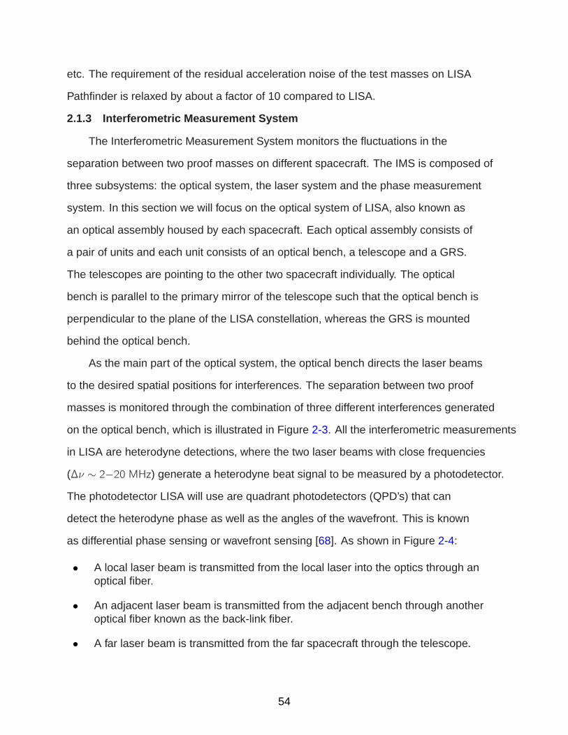
etc. The requirement of the residual acceleration noise of the test masses on LISA
Pathfinder is relaxed by about a factor of 10 compared to LISA.
2.1.3 Interferometric Measurement System
The Interferometric Measurement System monitors the fluctuations in the
separation between two proof masses on different spacecraft. The IMS is composed of
three subsystems: the optical system, the laser system and the phase measurement
system. In this section we will focus on the optical system of LISA, also known as
an optical assembly housed by each spacecraft. Each optical assembly consists of
a pair of units and each unit consists of an optical bench, a telescope and a GRS.
The telescopes are pointing to the other two spacecraft individually. The optical
bench is parallel to the primary mirror of the telescope such that the optical bench is
perpendicular to the plane of the LISA constellation, whereas the GRS is mounted
behind the optical bench.
As the main part of the optical system, the optical bench directs the laser beams
to the desired spatial positions for interferences. The separation between two proof
masses is monitored through the combination of three different interferences generated
on the optical bench, which is illustrated in Figure 2-3. All the interferometric measurements
in LISA are heterodyne detections, where the two laser beams with close frequencies
(∆ν ∼ 2−20 MHz) generate a heterodyne beat signal to be measured by a photodetector.
The photodetector LISA will use are quadrant photodetectors (QPD’s) that can
detect the heterodyne phase as well as the angles of the wavefront. This is known
as differential phase sensing or wavefront sensing [68]. As shown in Figure 2-4:
• A local laser beam is transmitted from the local laser into the optics through anoptical fiber.
• An adjacent laser beam is transmitted from the adjacent bench through anotheroptical fiber known as the back-link fiber.
• A far laser beam is transmitted from the far spacecraft through the telescope.
54

Figure 2-3. The Interferometric Measurement System of LISA. Each spacecraft housestwo optical benches, which transmit/receive laser beams to/from the othertwo spacecraft via telescopes, forming six one-way links. In this diagram onelaser (the “red” laser) on SC1 is used as the master laser, which ispre-stabilized to an optical cavity. The other five lasers are phase-lockedeither locally to the master laser via the back-link fiber or using the beatsignal with the far laser via optical transponders. The distance between twoproof masses on each arm is monitored by three distinct measurements:one measurement between optical benches (long arm) and twomeasurements between each proof mass and its respective optical bench(short arm + reference).
55

Figure 2-4. Interferometers on the optical bench of LISA. The interferometry used inLISA is heterodyne detections, where two lasers with close frequencies arecombined to generate a beat signal with its phase detected at thephotodetector. On each optical bench three interferometers are constructedusing three photodetectors and their measurements are combined tomeasure the distance between two proof masses on each arm. Note thatthis is just an oversimplified diagram to illustrate the interferometers,whereas there are also non-interferometric beams propagating through theoptical bench. Also, the GRS and its housed proof mass are actually not inthe plane of the optical bench.
Figure 2-3 shows that the adjacent beam and the original local beam generate a
heterodyne interference at the photodiode PDR, which measures the relative phase
noise of the two lasers and the additional noise introduced by the back-link fiber.
This measurement is known as the reference measurement. The adjacent beam is
also be superimposed onto the local beam that is reflected off from the proof mass.
This interference that occurs at the photodiode PDS is monitored as the short arm
measurement, which contains the fluctuation information of the distance from the
proof mass to the optical bench [69]. Therefore, the short arm interferometer of LISA
is also called the test mass interferometer, where the readout can be sent to the DRS
to actively control the motion of the proof mass in corporation with capacitive sensing.
The third kind of interference that occurs between the local beam and the received
and delayed far beam is recorded by the photodiode PDL. This beat note carries the
56

fluctuation information of the LISA long arm length from a local optical bench to a
far optical bench, which is known as the long arm measurement. Since the long arm
interferometer is used to detect the length fluctuations due to gravitational waves, it
is also referred to as the science interferometer. Therefore, we can write down the
photodiode readouts of these three interferences:
• Reference measurement: ϕR(t) = Φl(t)−Φa(t) + Na(t)
• Short arm measurement: ϕS(t) = Φl(t)−Φa(t) + 2πλ∆Lpm(t) + Na(t)
• Long arm measurement: ϕL(t) = Φl(t)−Φf(t − τji(t)) + NTrans(t − τji(t)) + hji(t).
In the above expressions other uncorrelated noise such as shot noise introduced at
the photodiode and the technical noise introduced at the phasemeter ADCs are ignored.
Φl(t), Φa(t) and Φf(t) are the phases of the local beam, the adjacent beam and the far
beam, respectively. Na(t) contains the noise in the back-link fiber. ∆Lpm(t) is the relative
position between the proof mass and the optical bench. The light travel time from SCj to
SCi τji(t) is a function of time ascribed to the relative motion between spacecraft. The
transponder noise, NTrans(t), primarily includes the phase-locked loop noise from far
spacecraft. hji(t) is the phase fluctuation due to the incident gravitational wave strain
applied on the LISA long arm length (optical bench to optical bench).
Although the laser phase noise dominates in all three measured phases, the
linear combination of the reference measurement and the short arm measurement,
ϕS(t) − ϕR(t), eliminates the laser phase noise in Φl(t) and Φa(t), as well as the
additional noise Na(t). Thus the only remaining term 2πλ∆Lpm(t) represents the relative
position of the proof mass.
However, a more complicated version of this noise cancellation scheme is used
for the case of long arm interferometry, where the existence of delay time prevents
the laser phase noise from being automatically eliminated. Due to the significant
inequality between arm length which varies over time, the laser phase noise on two
long arms becomes uncorrelated and no longer cancels out in a standard Michelson
57

combination, not to mention that the transponder noises on two long arms are
intrinsically uncorrelated. The technique to solve this problem is known as Time Delay
Interferometry [70, 71]. As a post-processing algorithm, TDI synthesizes equal-armed
Michelson interferometry by time-shifting the interferometry signal data properly such
that the laser phase noise, clock transfer noise, bench motion, etc., are canceled out in
certain linear combinations. More details of TDI will be seen in the next section.
In addition to the three basic interferometers described above, the optical bench
also includes the point-ahead angle mechanism (PAAM). The PAAM ensures that in
the long arm interferometry the direction of the transmitted beam is not changed when
received by the far photodetector due to the transverse relative motion of the spacecraft.
The transverse component of the velocity is time-dependent; therefore, the PAAM is
required to be an on-board technique to correct the time-varying deviation angle. It
is estimated that this time-varying angle will accurately track the orbital motion of the
constellation. Consequently, the correction mechanism can be implemented before
launch and a feedback control loop is not necessary.
The telescope is another crucial component of the optical assembly that is used
to transmit laser fields in the long arm interferometry. The telescope for LISA will use
an off-axis Cassegrain reflector design with a magnification of 80x . Each telescope is
pointing to the corresponding far spacecraft to gather the incoming beam (∼ 100 pW)
as well as to expand and collimate the outgoing beam (∼ 1 W). The laser beam from
the local optical bench will be focused onto the secondary mirror, where it is magnified
and reflected to the primary mirror. From the primary mirror the collimated beam will be
sent to the far optical bench, where a reverse process will be performed. The design of
the telescope determines the power of the received beam and thereby the shot noise
limit for the IMS. The mechanical stability of the pathlength between the primary and the
secondary mirror is critical as the pathlength noise will directly enter the readout of the
58

long arm interferometer. Given the total IMS noise budget of 18 pm Hz−1/2, the required
pathlength stability for the telescope is no more than 1 pm Hz−1/2.
2.2 Noise Cancellation for LISA
LISA will use lasers with a wavelength of probably around 1 µm. The laser will
have to have frequency actuation capabilities sufficient to meet the LISA frequency
noise requirements. For quite a long time, the laser frequency control has been
a significant and complicated topic in studies on the long arm interferometry. In a
laser interferometric measurement, the laser frequency noise is required to cause an
equivalent noise no higher than the quantity to be measured. In the IMS noise budget,
the allocated pathlength noise for the laser frequency is 2 pm Hz−1/2, corresponding to
a laser phase noise below 1.2 × 10⁻⁵ cycles Hz−1/2 or a laser frequency noise below
5.6 × 10⁻⁶ Hz Hz−1/2. Since the arm lengths of the LISA constellation are inherently
unequal to each other and also time-varying, the laser frequency noise does not cancel
out in a standard Michelson-like way. In comparison, the typical frequency noise of
a free-running laser is on the level of 10 kHz/f Hz Hz−1/2, which requires the laser
frequency noise to be reduced by more than 12 orders of magnitude at 3 mHz.
Current understanding of the laser frequency control gives a three-level approach to
mitigate the frequency noise [72]. The first two steps are active stabilization techniques
and the third step is a post-processing technique. The laser frequency will first be
actively stabilized to a local reference on spacecraft (pre-stabilization), then stabilized
to the LISA arm (arm locking) and finally get canceled out to the requirement in the
post-processing (TDI).
2.2.1 Time Delay Interferometry
The concept of Time Delay Interferometry (TDI) is to synthesize interferometry
(TDI observables) by linearly combining phase measurements of single links and
appropriately time-shifting the measurement data during post-processing [11, 73].
As an algorithm in the time domain, TDI is capable of eliminating the laser phase
59

noise, differential clock noise and spacecraft motions in the long arm interferometry
while maintaining the phase fluctuations due to gravitational wave strains. The noise
suppression performance of TDI is primarily limited by the arm length knowledge, which
determines the light travel time used for accurately time-shifting and fractional delaying
the measurement data.
The TDI algorithm that assumes fixed arm length between spacecraft, also known
as the first generation TDI or “TDI 1.0”, only exploits the phase measurements delayed
by the respective propagation distance to form TDI observables. The second generation
TDI or “TDI 2.0” takes the time-varying arm length caused by spacecraft relative motions
into account by time-shifting the phase measurements by multiples of the propagation
distance [70, 74]. A “TDI 3.0” algorithm which includes the relative accelerations
between spacecraft has also been conceptualized, but is unnecessary to meet the
LISA noise budget. The individual phase measurement can be linearly combined to
form various TDI observables, such as an unequal-armed Michelson interferometer
(X combination) or a Sagnac interferometer (ζ combination). In this section we will
introduce the basic Michelson X-combination with fixed arm length to explain the noise
cancellation in TDI.
2.2.1.1 Michelson X-combination
The Michelson X-combination exploits the phase measurements on four links to
form an equal-armed Michelson interferometer. It should be noted that the phase-locking
on the far spacecraft (or correlation between lasers) is not necessary for any kind of
TDI combinations; however, using optical transponders could simplify the Michelson
X-combination such that only the two phase readouts on SC1 are required. As shown in
Figure 2-5 (left), SC1 is used as the local spacecraft located at the vertex. Since the two
lasers on SC1 are phase-locked to each other via the back-link fiber, the local spacecraft
can be considered as the beamsplitter that generates two in-phase coherent beams in
a standard Michelson interferometer. The laser field Φ1(t) emitted from SC1 propagates
60

Figure 2-5. (Left) The Michelson X-combination in static TDI, where SC1 is used as abeamsplitter to generate two coherent beams and the laser beamstransmitted from SC2 and SC3 resemble the coherent light back reflectedfrom mirrors in a Michelson interferometer. In post-processing the beatsignals are delayed by a virtual round-trip travel time on the other arm, whichis illustrated as the dashed line. (Right) The Sagnac combination in staticTDI, where two coherent beams are transmitted from SC1 following aclockwise and counterclockwise closed trajectory. Due to the rotation of theconstellation, a travel time difference of ∼ 47 µs is generated. Similarpost-processing will be used to cancel out the laser frequency noise, clocknoise, etc.
through the long arm 1-2 and 1-3 individually and phase-locks the far laser on SC2 and
SC3. Therefore, the laser field transmitted from SC2 and SC3 resembles the coherent
light back reflected from mirrors in a Michelson interferometer. If we assume that the
far-end PLL yields a phase noise ϕPLLi(t), i = 2, 3, the phase measurement of the
heterodyne interferometry on SC1 is given by
Si(t) = Φ1(t)−Φ1(t − τ1i − τi1) + ϕPLLi(t − τi1) + h1i(t − τi1) + hi1(t), (2–6)
where τij is the one-way light travel time from SCi to SCj , h1i(t) and hi1(t) are phase
perturbations from gravitational waves. The linear combination of Michelson X is given
by
X (t) = S2(t)− S3(t)− S2(t − τ13 − τ31) + S3(t − τ12 − τ21). (2–7)
61

The additional terms can be interpreted as the beat signal Si(t) on SC1 delayed
by a virtual round-trip travel time on the other arm, which is illustrated as the dashed
line in Figure 2-5 (left). If we substitute Eq.2–7 with Eq.2–6, all phase noise terms
are canceled out. In principle, this algorithm reconstructs an equal-armed Michelson
interferometer and extract the common phase noise out of seemingly uncorrelated
phase measurements. The residual transponder noise from the far-end PLL will also be
measured on the far spacecraft. It is then appropriately time-shifted and subtracted from
the X-combination. Similar procedures will also be made for the removal of clock noise,
bench motion, back-link fiber noise, etc. On the other hand, the phase perturbations
from gravitational waves will be maintained in the post-processed signal, yielding
X (t) = h12(t − τ21) + h21(t)− h13(t − τ31)− h31(t)
− h12(t − τ21 − τ13 − τ31)− h21(t − τ13 − τ31)
+ h13(t − τ31 − τ12 − τ21) + h31(t − τ12 − τ21). (2–8)
Briefly speaking, the deduction from Eq. 2–6 to Eq. 2–8 demonstrates the basic
post-processing technique to extract gravitational waves from LISA readouts.
2.2.1.2 Sagnac combination
Another notable TDI observable is the Sagnac combination, which uses the LISA
signals to form a Sagnac interferometer [75]. A standard Sagnac interferometer consists
of a beamsplitter to generate two coherent beams, which propagate around a closed
loop in opposite directions and then are recombined at the beamsplitter. In LISA, six
links from three spacecraft are used to construct a Sagnac combination. As shown
in Figure 2-5 (right), the two coherent beams are transmitted from SC1 following a
clockwise and counterclockwise trajectory, respectively. Since the LISA constellation is
not static due to the rotation, a light path difference ∆L between the two propagations in
62

opposite directions is generated. This is known as the Sagnac effect:
∆L = L12 + L23 + L31 − (L13 + L32 + L21) =4Ω · Ac. (2–9)
In this equation Ω is the angular velocity of the rotation and A is the area enclosed
by the lightpath. The angular velocity of the LISA constellation is given by 1 cycle/year,
corresponding to 2 × 10⁻⁷ rad/s. Given that the constellation is inclined by 60 with
respect to the ecliptic, the parallel component of the angular velocity is only half of the
magnitude. Therefore, the lightpath difference is approximately ∆L ≈ 14.4 km, which is
equivalent to a propagation time difference of approximately 47 µs.
If we assume the phase noise from all phase-locked loops in the constellation is
zero, in the clockwise trajectory the phase measurements are given by
φ23(t) = φ12(t − τ12)− h12(t),
φ31(t) = φ23(t − τ23)− h23(t),
S13(t) = φ13(t)− φ31(t − τ31) + h31(t). (2–10)
Thus we obtain
S13(t) = φ13(t)−φ12(t− τ12− τ23− τ31)+h12(t− τ23− τ31)+h23(t− τ31)+h31(t). (2–11)
By following the same procedure, the other phase measurement on SC1 is given by
S12(t) = φ12(t)−φ13(t− τ13− τ32− τ21)+h13(t− τ32− τ21)+h32(t− τ21)+h21(t). (2–12)
Since the difference between the clockwise propagation time τCW = τ12 + τ23 + τ31
and the counterclockwise propagation time τCCW = τ13+ τ32+ τ21 is ∼ 47 µs, we still need
time-shifting to cancel out the arm length difference.
2.2.1.3 TDI Limitations
The TDI capability of noise suppression is limited by several realistic effects,
primarily the arm length knowledge which directly depends on the ranging accuracy.
63

In addition to the ranging accuracy, limiting effects include the velocity correction error,
analog chain error 1 , phasemeter noise and scattered light, etc.
The ranging system LISA will use is pseudo-random noise (PRN) ranging, which
phase modulates the carrier of the far laser with a PRN code stream. The travel time
then can be measured via the correlation between the local and received PRN code.
Current estimation of the PRN ranging error is δL ≈ 1 m (∼ 1 ns in terms of timing error).
Allocated by the IMS noise budget, the residual laser frequency noise at the TDI
output is required to be below 2 pmHz−1/2 ×√1 + (2.8 mHz/f)4. With a 1 m ranging
accuracy, the required laser frequency noise at the TDI input is given by
δνpre−TDI(f ) < 282×
√
1 +
(2.8 mHz
f
)4Hz Hz−1/2. (2–13)
In comparison to the noise suppression limited by ranging, other limiting effects yield
more relaxed requirements for δνpre−TDI, which indicates the ranging accuracy on LISA
arm length is the dominant limitation for TDI. Due to the limited ranging accuracy, TDI
would not meet the 2 pm requirement on residual laser frequency noise by itself, since a
free-running laser typically carries frequency noise on the level of 10 kHz/f Hz Hz−1/2.
This frequency noise is several orders of magnitude beyond the stability specified in
Eq. 2–13; therefore, the laser frequency must be actively pre-stabilized to achieve the
requirement.
2.2.2 Pre-stabilization
The frequency stabilization plan is to lock the laser frequency to a stable reference.
On the local spacecraft, such a stable reference can be either a high-finesse Fabry-Perot
cavity made of ultra-low expansion glass or an atomic or molecular spectral line [76].
The modulation-demodulation method uses an optical cavity known as Pound-Drever-Hall
1 The analog chain consists of a photoreceiver, a pre-amplifier and an anti-aliasingfilter successively placed before the ADCs.
64

Figure 2-6. The experimental setup of Pound-Drever-Hall stabilization.
(PDH) technique [77]. It has been well studied in laboratory, giving a frequency
noise suppression performance of ∼ 30 Hz/√Hz at 3 mHz [78]. Besides the widely
favored PDH technique, another pre-stabilization method is based on a heterodyne
Mach-Zehnder interferometer, which exploits the pathlength mismatch between two
different lasers as the frequency reference. This method has been used in the LISA
Technology Package (LTP) for LISA Pathfinder [79]. Note that in all six lasers only
one master laser is needed to be pre-stabilized using one of the methods described
above, and the other five lasers are stabilized using phase-locking either locally to the
master laser via the back-link fiber or using the beat signal with the far laser via optical
transponders.
2.2.2.1 Pound-Drever-Hall frequency stabilization
The Pound-Drever-Hall technique is the most used frequency stabilization method in
optical experiments [80]. The optical cavity used in laboratory is normally a high-finesse
(∼ 104) Fabry-Perot cavity, which consists of two low-loss mirrors bonded to a rigid
spacer made of low-expansion material such as Zerodur or ULE. As shown in Figure
2-6, the laser beam with a nominal frequency ω is transmitted through an electro-optical
modulator (EOM) driven by a local oscillator with a nominal frequency Ω (typically
> 5 MHz, well larger than the FWHM of the cavity), producing two sidebands ω ± Ω.
65

After the polarizing beam splitter and the quarter-wave plate, the beam is reflected from
the optical cavity. We use the reflected beam to feedback control the laser frequency.
The reflectivity Tr of an optical cavity is a function of the laser frequency ω:
Tr(ω) ≡Er(ω)
Ei(ω)=r1 − r2e iϕ1− r1r2e iϕ
, (2–14)
where ϕ = 2ωL/c is the phase shift due to a round-trip inside the cavity. r1, r2, t1 and
t2 are the reflection coefficients and transmission coefficients of mirror 1 and 2 and we
assume a lossless cavity with r 21 + t21 = 1.
If the carrier frequency of the beam exactly matches up the resonant frequency of
the cavity ωL = 2πnc/L, the reflected carrier will have zero phase shift. Also, as long as
Ω is large enough such that the sidebands are far away from the resonant frequency,
their phase shift will be negligible. Therefore, the reflected carrier will generate two
heterodyne beat signals with each sideband. Since they are 180 out of phase, the
superposition of them on the photodiode would be zero.
If the carrier frequency is slightly off the resonant frequency, a phase shift will be
generated in the reflected carrier. When the offset δω to the resonant frequency is small,
the reflectivity transfer function approximates to the first linear order by taking Taylor
expansion:
Tr(δω) =r1 − r21− r1r2
+ 2ir 21 r2 − r2(1− r1r2)2
δωL
c
=r1 − r21− r1r2
− 2iF δν
FSR
=r1 − r21− r1r2
− i δν
HWHM. (2–15)
In other words, the cavity is able to detect whether the carrier frequency is above
or below the resonant frequency since the sign of the phase shift depends on the sign
of the frequency offset. Also due to the phase shift, the heterodyne beat signals will
no longer cancel out each other. If we demodulate the reflected beam with the same
66

oscillator Ω and low-pass filter the high frequency component, a zero-crossing DC signal
that is linear with respect to the frequency offset can be generated to feedback control
the laser frequency.
In the LISA band especially below 1 mHz, the frequency stability of the PDH
technique is mainly limited by the temperature fluctuations that causes spurious noises
in the cavity length. The relative stability ∆L/L of the referencing cavity length in our
experiments is as low as 10−13, resulting in a frequency noise of about 30 Hz Hz−1/2.
2.2.2.2 Mach-Zehnder frequency stabilization
Mach-Zehnder frequency stabilization requires a dedicated heterodyne interferometer
with unequal arm, which is used as the frequency reference. In the LTP baseline design
the unequal-armed Mach-Zehnder interferometer is configured using a beam splitter
and two acousto-optic modulators (AOM) to generate heterodyne interferometry signals
at 1 − 2 kHz [81, 82]. On the LISA optical bench, the integration of such a heterodyne
interferometer becomes easier as the interferometry signal between two adjacent
lasers is already incorporated into the phase readout. Compared with stabilization to a
Fabry-Perot cavity, Mach-Zehnder stabilization simplifies the optical bench setup, where
neither an optical cavity nor an EOM is not necessary to be implemented. Also, this
pre-stabilization method allows to tune the laser frequency over a wide range without the
necessity of changing the pathlength mismatch.
The proposed interferometer setup is illustrated by Figure 2-7. Between the
two adjacent lasers on the same spacecraft, one laser marked as the slave laser is
phase-locked to the master laser with a frequency offset (2− 20 MHz) driven by the local
oscillator. As we already know, the heterodyne interferometry signal between them is
measured at the photodiode PDR and the phase readout is given by
ϕR = ΦS −ΦM. (2–16)
67

Figure 2-7. The interferometer setup for Mach-Zehnder frequency stabilization. In thissetup the slave laser is heterodyne phase-locked to the master laser. Theirheterodyne signal ϕR is measured at the reference photodiode. The otherarm of the Mach-Zehnder interferometer has an additional pathlength L,which generates a propagation delay in the heterodyne signal ϕF. The errorsignal of Mach-Zehnder stabilization is given by ϕF − ϕR, which exploits thepathlength mismatch as a reference to stabilize the master laser. Note thatthe mixers in this diagram may represent phasemeters, each driven by acommon local oscillator. The phasemeters demodulate the heterodynesignals with the same offset frequency and measure the phase noise in eachof them.
Based on the dynamics of the PLL, in the Laplace domain the phase noise ΦS of the
phase-locked slave laser is given by
ΦS =1
1 + G1Φ0S +
G1
1 + G1ΦM. (2–17)
The first term represents the noise suppression of the free-running slave laser and
the second terms indicates that the phase noise of the slave laser tracks the phase
noise of the referenced master laser. Therefore, the phase measurement at PDR can be
written as
ϕR =1
1 + G1Φ0S −
1
1 + G1ΦM. (2–18)
68
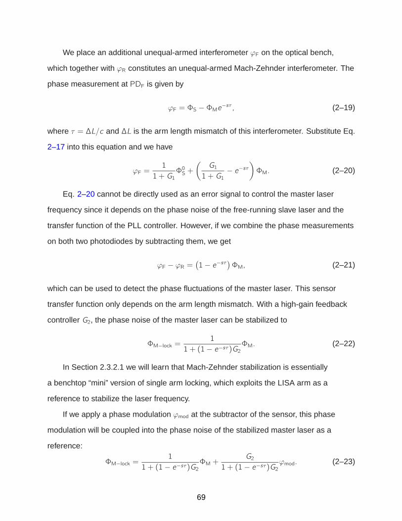
We place an additional unequal-armed interferometer ϕF on the optical bench,
which together with ϕR constitutes an unequal-armed Mach-Zehnder interferometer. The
phase measurement at PDF is given by
ϕF = ΦS −ΦMe−sτ , (2–19)
where τ = ∆L/c and ∆L is the arm length mismatch of this interferometer. Substitute Eq.
2–17 into this equation and we have
ϕF =1
1 + G1Φ0S +
(G1
1 + G1− e−sτ
)ΦM. (2–20)
Eq. 2–20 cannot be directly used as an error signal to control the master laser
frequency since it depends on the phase noise of the free-running slave laser and the
transfer function of the PLL controller. However, if we combine the phase measurements
on both two photodiodes by subtracting them, we get
ϕF − ϕR =(1− e−sτ
)ΦM, (2–21)
which can be used to detect the phase fluctuations of the master laser. This sensor
transfer function only depends on the arm length mismatch. With a high-gain feedback
controller G2, the phase noise of the master laser can be stabilized to
ΦM−lock =1
1 + (1− e−sτ)G2ΦM. (2–22)
In Section 2.3.2.1 we will learn that Mach-Zehnder stabilization is essentially
a benchtop “mini” version of single arm locking, which exploits the LISA arm as a
reference to stabilize the laser frequency.
If we apply a phase modulation ϕmod at the subtractor of the sensor, this phase
modulation will be coupled into the phase noise of the stabilized master laser as a
reference:
ΦM−lock =1
1 + (1− e−sτ)G2ΦM +
G2
1 + (1− e−sτ)G2ϕmod. (2–23)
69

Thus we have∂ΦM−lock∂ϕmod
=G2
1 + (1− e−sτ)G2. (2–24)
It is easy to demonstrate that in the high gain limit (G2 ≫ 1), Eq. 2–24 approximates
to∂ΦM−lock∂ϕmod
≈ 1
sτ. (2–25)
The above relation holds for frequencies much lower than 1/τ , which is always valid
in the locking bandwidth (∼ 20 Hz). In terms of frequency, it can be represented as
∂νM−lock∂ϕmod
≈ 1τ, (2–26)
which indicates the frequency of the master laser can be continuously tuned by
introducing a phase offset ϕmod at the sensor. The actuation factor from the phase
modulation to the frequency tuning is given by 1/τ .
The noise performance of Mach-Zehnder stabilization is limited by the pathlength
stability of the interferometer, as well as sensing noise sources introduced by the
photodiodes and phasemeters (shot noise, digitization noise, etc.) If we assume the
sensing noise is equivalent to 1 pm/√Hz, for a 0.5 m pathlength mismatch the expected
stabilized frequency noise is approximately given by
δνMZ = 800×
√
1 +
(2.8 mHz
f
)4Hz Hz−1/2. (2–27)
Although this expected performance is inferior to the fixed cavity and does not
meet the requirement for pre-stabilization, Mach-Zehnder stabilization provides an
intrinsic frequency tunability that the PDH stabilization does not have, which makes
the incorporation of Mach-Zehnder stabilization with arm locking much easier. The
incorporation can be achieved by adjusting the phase of the local oscillator that is used
to demodulate the Mach-Zehnder heterodyne signal through arm locking. More details
of the integration of Mach-Zehnder stabilization and arm locking will be seen in Section
70

2.3.4.2. In addition, a variation of Mach-Zehnder stabilization that uses a Fabry-Perot
cavity to achieve the arm length mismatch has also been developed. Due to the better
stability of the cavity length, the stabilization performance is expected to be superior to
the standard Mach-Zehnder method, which has been demonstrated in relevant benchtop
experiments [83].
2.3 Arm Locking
In comparison to Mach-Zehnder stabilization that exploits the path length to
the adjacent optical bench as a reference, the LISA long arm (from optical bench to
optical bench) is another path length reference which provides a even better stability
(δL/L ∼ 10−21 Hz−1/2) in the LISA band. Techniques that transfer the stability of the
long arm lengths to the laser frequency are generally known as arm locking. Unlike
Mach-Zehnder stabilization that requires an extra interference path in the setup, the
arm locking architecture is intrinsically embedded in the LISA constellation: Arm locking
synthesizes the error signal from the inter-spacecraft phase measurements, which are
already available at the photodetectors. This feature allows that the control system of
arm locking can be fully implemented in on-board data processing and no additional
resource is needed. With constellation phase locking on far spacecraft, the local laser
beam has an interference with its replica delayed by the light round-trip travel time
τ ≈ 33 s. Such a long time delay is very uncommon in ordinary sensors, as it may
cause excessive phase shift at interferometer null frequencies and then limit the control
bandwidth. However, the pioneering work done by Sheard et al has demonstrated that
the bandwidth of arm locking is not necessarily limited by the long time delay and a
high gain controller design is achievable if the phase margin is carefully retained [84].
More studies on arm locking have analytically demonstrated that the instantaneous
phase information can be recovered via an adequate linear combination of phase
measurements.
71

Figure 2-8. The baseline design of arm locking. The laser field of Laser 1 (L1) on thelocal SC1 is split and sent to the far SC2 and SC3. The laser fields of Laser 2(L2) and Laser 3 (L3) are phase-locked to the incoming field of L1 andtransmitted back to SC1. On SC1 the phase-locked laser fields of L2 and L3are demodulated by the instantaneous laser field of L1. These two beatsignals are measured by two phasemeters individually. Arm locking takes alinear combination of these two phase measurements to estimate the phasenoise information, which is then used to control the frequency of L1.
2.3.1 Architecture
The basic schematic of arm locking in LISA is illustrated in Figure 2-8. In this
diagram, one spacecraft SC1 is used as a local or master spacecraft on which the laser
is pre-stabilized by locking to a local frequency reference. When the laser field from SC1
is transmitted to either of the two far spacecraft SC2 and SC3, the laser on them will be
phase-locked by the controller G2,3 to the incoming laser. If we assume the initial phase
72
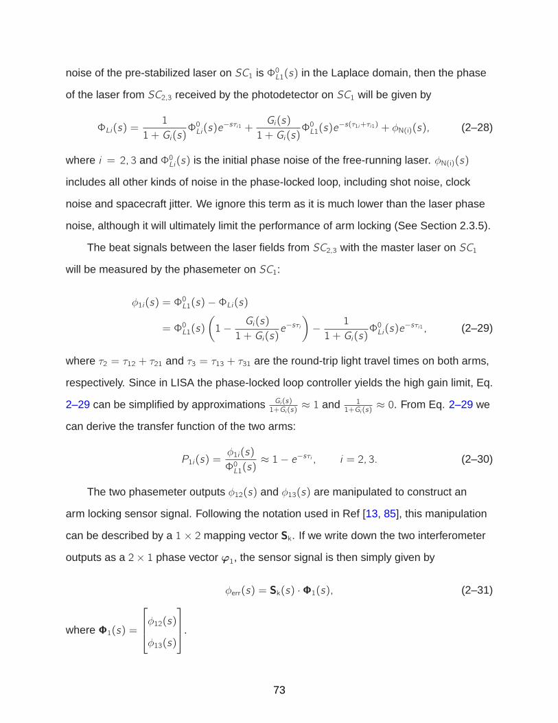
noise of the pre-stabilized laser on SC1 is Φ0L1(s) in the Laplace domain, then the phase
of the laser from SC2,3 received by the photodetector on SC1 will be given by
ΦLi(s) =1
1 + Gi(s)Φ0Li(s)e
−sτi1 +Gi(s)
1 + Gi(s)Φ0L1(s)e
−s(τ1i+τi1) + φN(i)(s), (2–28)
where i = 2, 3 and Φ0Li(s) is the initial phase noise of the free-running laser. φN(i)(s)
includes all other kinds of noise in the phase-locked loop, including shot noise, clock
noise and spacecraft jitter. We ignore this term as it is much lower than the laser phase
noise, although it will ultimately limit the performance of arm locking (See Section 2.3.5).
The beat signals between the laser fields from SC2,3 with the master laser on SC1
will be measured by the phasemeter on SC1:
φ1i(s) = Φ0L1(s)−ΦLi(s)
= Φ0L1(s)
(1− Gi(s)
1 + Gi(s)e−sτi
)− 1
1 + Gi(s)Φ0Li(s)e
−sτi1, (2–29)
where τ2 = τ12 + τ21 and τ3 = τ13 + τ31 are the round-trip light travel times on both arms,
respectively. Since in LISA the phase-locked loop controller yields the high gain limit, Eq.
2–29 can be simplified by approximations Gi (s)1+Gi (s)
≈ 1 and 11+Gi (s)
≈ 0. From Eq. 2–29 we
can derive the transfer function of the two arms:
P1i(s) =φ1i(s)
Φ0L1(s)≈ 1− e−sτi , i = 2, 3. (2–30)
The two phasemeter outputs φ12(s) and φ13(s) are manipulated to construct an
arm locking sensor signal. Following the notation used in Ref [13, 85], this manipulation
can be described by a 1 × 2 mapping vector Sk. If we write down the two interferometer
outputs as a 2× 1 phase vector ϕ1, the sensor signal is then simply given by
φerr(s) = Sk(s) ·Φ1(s), (2–31)
where Φ1(s) =
φ12(s)
φ13(s)
.
73

When the arm locking loop is closed, the phase noise at the local laser output is
given by
ΦL1(s) = Φ0L1(s)−
G1(s)
1 + G1(s)H(s)Sk ·Φ1(s)
=Φ0L1(s)
1 + G1(s)H(s), (2–32)
where G1(s) is the arm locking controller and
H(s) = Sk(s) ·
P12(s)
P13(s)
(2–33)
is the arm locking sensor. Compared with the initial phase noise of the pre-stabilized
laser, the stabilized phase noise is suppressed by the open-loop gain G1(s)H(s).
2.3.2 Arm Locking Sensors
2.3.2.1 Single arm locking
Single arm locking is the original idea of arm locking proposed by Sheard et al.. In
the single arm locking configuration only the interferometer output on one arm will be
used and consequently we have HS(s) = P12(s) = 1− e−sτ2. As shown in Figure 2-9, the
sensor transfer function has zero magnitude response at DC as well as at frequencies
n/τ2 known as nulls. The phase response starts from a 90 phase advance at DC and
has discontinuities at these nulls where the phase jumps from −90 to 90. The transfer
function also have multiple unity gain frequencies, on both sides near each null.
These unity gain frequencies place additional stability constraints on the controller
design. In practice an integrator with a single pole at DC is widely used in feedback
controllers as it provides a high gain at DC and the gain declines with a 1/s slope at high
frequencies, which is required by the limited bandwidth. However, this kind of controller
essentially does not work for single arm locking because the 1/s slope would bring in an
additional 90 phase shift. As the loop gain increases, the phase margin will be further
decreased, which will destroy the system stability. This problem is illustrated by Figure
74

10−4
10−3
10−2
10−1
100
0
1
2
Frequency (Hz)
Mag
nitu
de
10−4
10−3
10−2
10−1
100
−100
0
100
Frequency (Hz)
Pha
se s
hift
(deg
ree)
Figure 2-9. The magnitude and phase response of the single arm locking sensor. Notethat for the magnitude response we are not using the logarithmic scale in they axis (as we do in most cases) just to show the situation near interferometernulls more clearly. In the logarithmic scale the magnitude response versusthe Fourier frequency actually approximates to an f slope at lowfrequencies.
2-10, where the open-loop transfer function is given by the single arm locking sensor
multiplied by a 1/s slope. With a gain factor of 10, at the unity gain frequencies the
phase shift is already very close to 180.
To avoid losing excessive phase in bandwidth, the proposed design of the
controller has to have a slope less steep than 1/s to compensate the phase loss at
zero crossings. For instance, a 1/s1/2 or 1/s2/3 slope will only bring in a 45 or 60 phase
shift, respectively. We assume a generic arm locking controller filter with the transfer
function G(f ) = kf −αe iϕ, where 0 < α < 1, k is a real gain factor and ϕ is the phase
shift introduced by the filter. As we know, the closed-loop transfer function of a feedback
control loop is defined as
TFCL(f ) ≡φout(f )
φin(f )≡ 1
1 + TFOL(f ). (2–34)
75
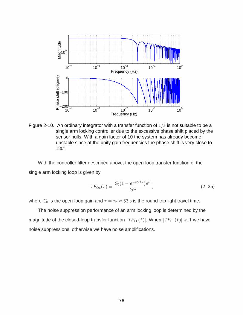
10−4
10−3
10−2
10−1
100
100
Frequency (Hz)
Mag
nitu
de
10−4
10−3
10−2
10−1
100
−200
−100
0
Frequency (Hz)
Pha
se s
hift
(deg
ree)
Figure 2-10. An ordinary integrator with a transfer function of 1/s is not suitable to be asingle arm locking controller due to the excessive phase shift placed by thesensor nulls. With a gain factor of 10 the system has already becomeunstable since at the unity gain frequencies the phase shift is very close to180.
With the controller filter described above, the open-loop transfer function of the
single arm locking loop is given by
TFOL(f ) =G0(1− e−i2πf τ)e iϕ
kf α, (2–35)
where G0 is the open-loop gain and τ = τ2 ≈ 33 s is the round-trip light travel time.
The noise suppression performance of an arm locking loop is determined by the
magnitude of the closed-loop transfer function |TFCL(f )|. When |TFCL(f )| < 1 we have
noise suppressions, otherwise we have noise amplifications.
76

If we substitute Eq. 2–35 into Eq. 2–34 and evaluate the magnitude of the
closed-loop transfer function |TFCL(f )|, it yields
|TFCL(f )| =∣∣∣∣
kf αe iϕ
kf αe iϕ + G0(1− e−i2πf τ)
∣∣∣∣
=
√k2f 2α
k2f 2α + 2G 20 (1− cos 2πf τ)− 2kG0f α(cos(ϕ+ 2πf τ)− cosϕ)
=
√k2f 2α
k2f 2α + ∆. (2–36)
From the result of Eq. 2–36, the noise suppression performance depends on the value
of
∆ = 2G 20 (1− cos 2πf τ)− 2kG0f α(cos(ϕ+ 2πf τ)− cosϕ), (2–37)
i.e., ∆ > 0, ∆ = 0, ∆ < 0 corresponds to the case of noise suppression, no suppression
and noise amplification, respectively. 2
A specific model to numerically evaluate ∆ is shown in Figure 2-11. In this system
model we assume the loop gain G0 = 10 and the filter has a magnitude response
|G(f )| = 1/f 1/2 with a 45 phase shift. The plot shows that in the frequency region
f ≪ 1/τ , we have ∆ ≈ 0, which means a simple 1/f α slope does not provide any noise
suppression at DC. This can also be seen from the transfer function of the single arm
locking sensor, which has a f slope starting from DC. To overcome this f slope in the
sensor and obtain some noise suppression at DC, the controller must have at least a
1/f slope in the frequency region f ≪ 1/τ .
In the frequency region where f is comparable to n/τ , ∆ is generally larger than
zero but with a few exceptions. At some certain frequencies which are very close to
2 From the point of view of mathematics, the value of ∆ is obviously required to have alower limit: ∆ > −k2f 2α, otherwise the expression of the magnitude response would notbe meaningful. In practice, the value of ∆ generally meets this requirement in the LISAband since the Fourier frequency is low.
77

10−4
10−3
10−2
10−1
100
0
200
400
Frequency (Hz)
10−4
10−3
10−2
10−1
100
−0.2
0
0.2
Frequency (Hz)
Figure 2-11. An example of the value of ∆ that indicates the noise suppression, which isgiven by Eq. 2–37. Larger value of ∆ indicates more noise suppressions.Note that in this model we did not include integrators at low frequencies;therefore we do not have any suppression at DC. The value of ∆ can benegative at certain frequencies near each null, corresponding to noiseamplifications due to the excessive phase loss.
each null n/τ , numerical calculation shows that ∆ can be less than zero, causing noise
amplifications at these frequencies. These noise amplifications correspond to multiple
peaks with finite heights in the closed-loop transfer function as shown in Figure 2-12.
It is worth noting that noise amplifications do not occur exactly at sensor nulls n/τ .
Actually when f = n/τ , ∆ = 0 and the control loop has no noise suppressions or
amplifications.
As shown in Figure 2-12, an ideal single arm-locking controller would be designed
in the following manner: starting from DC the filter has a steep slope of at least 1/f to
suppress the low frequency noise and stops right before the first null 1/τ ; starting from
the first null the filter transfer function has a 1/f 1/2 or 1/f 2/3 slope in bandwidth and
starts to flatten out beyond the bandwidth.
Although the idea of single arm locking has been theoretically and experimentally
validated by multiple researchers, the shortcomings of single arm locking make it
78

10−4
10−3
10−2
10−1
100
10−4
10−3
10−2
10−1
100
101
Frequency (Hz)
Noi
se s
uppr
essi
on
Figure 2-12. An example of the closed-loop transfer function of single arm locking,where the light travel time is 33 s. The controller consists of a filter with a1/f 1/2 slope and two-stage integrators.
ultimately inappropriate for realistic LISA. It is very noticeable that the first null shows
up right inside the LISA band, which in any case is not an ideal noise suppression
performance due to the noise amplifications near the nulls. Moreover, since the first
null is in the LISA band, the gain around that region must be high enough to provide
a decent noise suppression. Considering the controller will have a slope less steep
than 1/f , an extremely large bandwidth would be needed in single arm locking.
The third disadvantage of single arm locking is the start-up transients caused by the
non-zero initial error signal, which creates the repeating 33 seconds noise with damped
oscillations [86, 87].
2.3.2.2 Common arm locking
Under most circumstances, the lengths of two LISA arms are different by a relatively
small amount except for some certain short periods. For this reason, common arm
locking, as the simplest arm locking configuration that utilizes the interferometer outputs
on both two arms, exploits the arm length mismatch to push the first null of the sensor
to higher frequencies beyond the LISA band. As Markus Herz pointed out using the
79

0 500 1000 1500 2000 2500−0.4
−0.3
−0.2
−0.1
0
0.1
0.2
0.3
0.4
0.5
Time (s)
Pha
se v
aria
tion
(cyc
le)
Figure 2-13. The time domain simulation to demonstrate the initial transients in singlearm locking. The quasiperiodic transient is “frozen” inside the output signalwith a 33 s oscillation and decays with a time constant of approximately∼ 500 s for this specific model.
second arm allows to reduce the start-up transients[88]. The mapping vector Sk(s) of
common arm locking configuration is [1, 1], as it simply combines the two interferometer
outputs by adding them. Thus the sensor transfer function of common arm locking is
given by
HC(s) = P+(s) = [1, 1] ·
P12(s)
P13(s)
= P12(s) + P13(s)
= 2− e−sτ2 − e−sτ3. (2–38)
If we define τ ≡ (τ2 + τ3)/2 and ∆τ ≡ (τ2 − τ3)/2 > 0, the transfer function can also
be represented in the angular frequency by taking the transformation s = iω:
P+(ω) = 2[1− cos(∆τω)e−i τω]. (2–39)
This sensor transfer function resembles that of single arm locking HS(ω) = 1− e−iτω.
The difference is that the round-trip time on one arm is replaced by the averaged
80
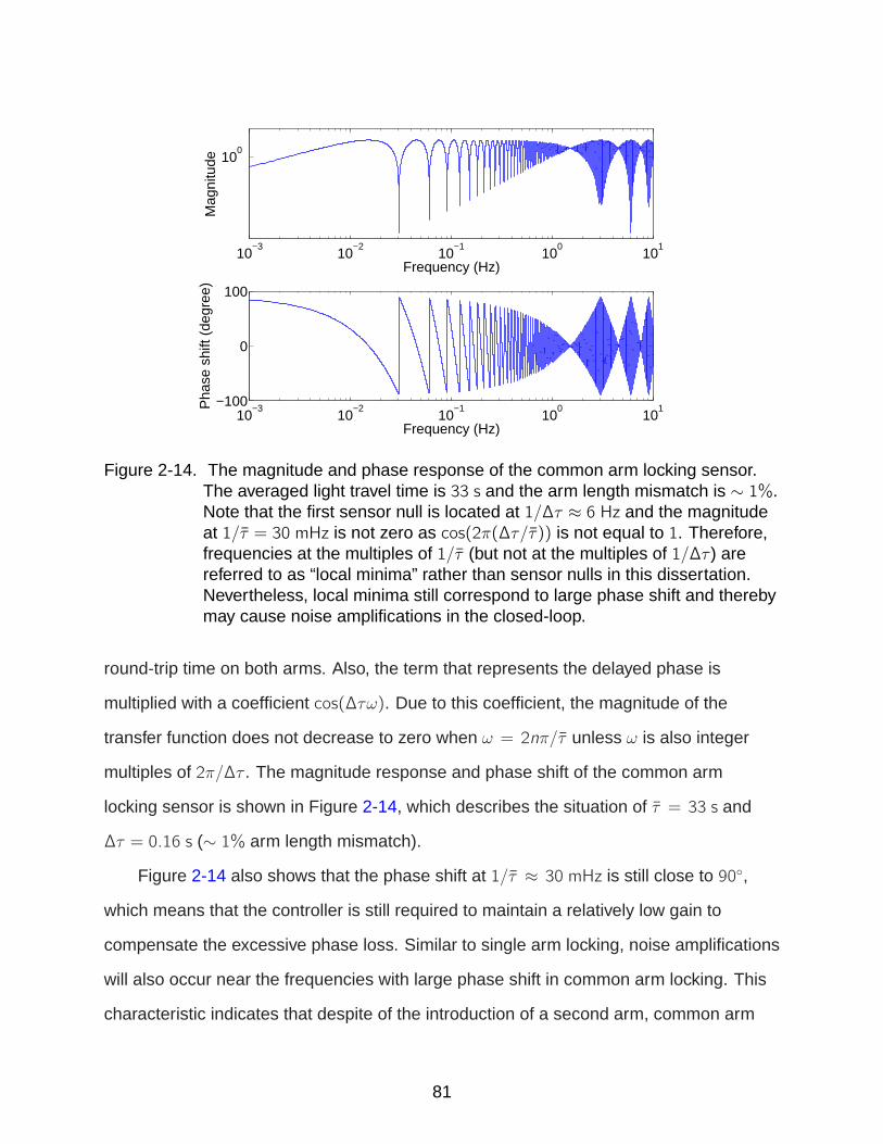
10−3
10−2
10−1
100
101
100
Frequency (Hz)
Mag
nitu
de
10−3
10−2
10−1
100
101
−100
0
100
Frequency (Hz)
Pha
se s
hift
(deg
ree)
Figure 2-14. The magnitude and phase response of the common arm locking sensor.The averaged light travel time is 33 s and the arm length mismatch is ∼ 1%.Note that the first sensor null is located at 1/∆τ ≈ 6 Hz and the magnitudeat 1/τ = 30 mHz is not zero as cos(2π(∆τ/τ)) is not equal to 1. Therefore,frequencies at the multiples of 1/τ (but not at the multiples of 1/∆τ ) arereferred to as “local minima” rather than sensor nulls in this dissertation.Nevertheless, local minima still correspond to large phase shift and therebymay cause noise amplifications in the closed-loop.
round-trip time on both arms. Also, the term that represents the delayed phase is
multiplied with a coefficient cos(∆τω). Due to this coefficient, the magnitude of the
transfer function does not decrease to zero when ω = 2nπ/τ unless ω is also integer
multiples of 2π/∆τ . The magnitude response and phase shift of the common arm
locking sensor is shown in Figure 2-14, which describes the situation of τ = 33 s and
∆τ = 0.16 s (∼ 1% arm length mismatch).
Figure 2-14 also shows that the phase shift at 1/τ ≈ 30 mHz is still close to 90,
which means that the controller is still required to maintain a relatively low gain to
compensate the excessive phase loss. Similar to single arm locking, noise amplifications
will also occur near the frequencies with large phase shift in common arm locking. This
characteristic indicates that despite of the introduction of a second arm, common arm
81

10−3
10−2
10−1
100
101
100
Frequency (Hz)
Mag
nitu
de
10−3
10−2
10−1
100
101
−200
0
200
Frequency (Hz)
Pha
se s
hift
(deg
ree)
differential armintegrated differential arm scaled by 1/∆ τ
Figure 2-15. The magnitude and phase response of the differential arm (green) and theintegrated differential arm scaled by 1/∆τ (red). The averaged light traveltime is 33 s and the arm length mismatch is ∼ 1%. They only contain theinformation of the delayed phase, therefore the maximum of their phaseshift is 180 and they cannot be solely used as an arm locking sensor.
locking is essentially not a significant improvement of single arm locking in terms of the
gain advantage and system stability.
2.3.2.3 Dual arm locking
Dual arm locking, also known as direct arm locking, combines the phase measurements
on two different arms and then directly provide a feedback signal by estimating the
instantaneous phase information. The original idea of dual arm locking is from Andrew
Sutton and Daniel Shaddock [85]. Compared with single arm locking and common arm
locking, dual arm locking exhibits several remarkable improvements such as no noise
amplification in the LISA band and significantly better noise suppression performance.
In addition to the common arm sensor described in Eq.(2-15), we can also define
the differential arm sensor:
P−(s) = P12(s)− P13(s) = e−sτ3 − e−sτ2. (2–40)
82

Again, when represented in the angular frequency domain, the differential arm
sensor is given by
Pω = 2i sin(∆τω)e−i τω, (2–41)
where the definitions of τ and ∆τ are the same as in the common arm sensor. We
plot the magnitude response and phase shift of the differential arm sensor in Figure
2-15.
The differential arm sensor only contains information of the purely delayed phase,
therefore it cannot be solely used for feedback control. However, the differential arm
signal can be linearly combined with the common arm signal in a certain way such that
the delayed term in the common arm sensor will be eliminated. In the Laplace domain,
such a linear combination is given by
H(s) = P+(s) +1
s∆τP−(s). (2–42)
Switched back to the angular frequency, the linear combination yields
H(ω) = 2− 2 cos(∆τω)e−i τω + 1∆τ
2i sin(∆τω)e−i τω
iω
= 2[1− (cos(∆τω)− sinc(∆τω)) e−i τω
]. (2–43)
At low frequencies (ω ≪ 1∆τ
), both cos(∆τω) and sinc(∆τω) are approximately
equal to 1. Therefore, the transfer function of this combination is approximately given
by H(ω) ≈ 2, i.e., the magnitude response retains almost flatness with a factor of 2 and
the phase shift is also almost entirely zero in the LISA band. In other words, this linear
combination extracts the instantaneous input phase from the interferometer outputs.
Due to the integration of the differential arm path, the differential arm sensor dominates
at low frequencies and the integrated differential arm retains the zero phase shift in this
region. The flat magnitude response and zero phase shift at low frequencies allow a
more flexible controller design, compared with the nulls at high frequencies that limit the
controller slope and therefore the achievable gain.
83
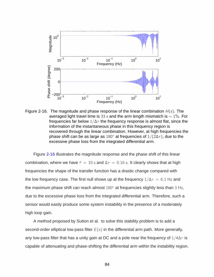
10−3
10−2
10−1
100
101
100
Frequency (Hz)
Mag
nitu
de
10−3
10−2
10−1
100
101
−200
0
200
Frequency (Hz)
Pha
se s
hift
(deg
ree)
Figure 2-16. The magnitude and phase response of the linear combination H(s). Theaveraged light travel time is 33 s and the arm length mismatch is ∼ 1%. Forfrequencies far below 1/∆τ the frequency response is almost flat, since theinformation of the instantaneous phase in this frequency region isrecovered through the linear combination. However, at high frequencies thephase shift can be as large as 180 at frequencies of 1/(2∆τ), due to theexcessive phase loss from the integrated differential arm.
Figure 2-16 illustrates the magnitude response and the phase shift of this linear
combination, where we have τ = 33 s and ∆τ = 0.16 s. It clearly shows that at high
frequencies the shape of the transfer function has a drastic change compared with
the low frequency case. The first null shows up at the frequency 1/∆τ = 6.1 Hz and
the maximum phase shift can reach almost 180 at frequencies slightly less than 3 Hz,
due to the excessive phase loss from the integrated differential arm. Therefore, such a
sensor would easily produce some system instability in the presence of a moderately
high loop gain.
A method proposed by Sutton et al. to solve this stability problem is to add a
second-order elliptical low-pass filter E(s) in the differential arm path. More generally,
any low-pass filter that has a unity gain at DC and a pole near the frequency of 1/4∆τ is
capable of attenuating and phase-shifting the differential arm within the instability region.
84
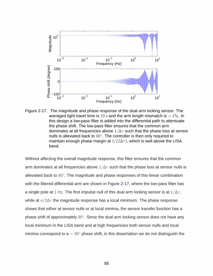
10−3
10−2
10−1
100
101
100
Frequency (Hz)
Mag
nitu
de
10−3
10−2
10−1
100
101
−100
0
100
Frequency (Hz)
Pha
se s
hift
(deg
ree)
Figure 2-17. The magnitude and phase response of the dual arm locking sensor. Theaveraged light travel time is 33 s and the arm length mismatch is ∼ 1%. Inthis design a low-pass filter is added into the differential path to attentuatethe phase shift. The low-pass filter ensures that the common armdominates at all frequencies above 1/∆τ such that the phase loss at sensornulls is alleviated back to 90. The controller is then only required tomaintain enough phase margin at 1/(2∆τ), which is well above the LISAband.
Without affecting the overall magnitude response, this filter ensures that the common
arm dominates at all frequencies above 1/∆τ such that the phase loss at sensor nulls is
alleviated back to 90. The magnitude and phase responses of this linear combination
with the filtered differential arm are shown in Figure 2-17, where the low-pass filter has
a single pole at 1 Hz. The first impulse null of this dual arm locking sensor is at 1/∆τ ,
while at n/2∆τ the magnitude response has a local minimum. The phase response
shows that either at sensor nulls or at local minima, the sensor transfer function has a
phase shift of approximately 90. Since the dual arm locking sensor does not have any
local minimum in the LISA band and at high frequencies both sensor nulls and local
minima correspond to a ∼ 90 phase shift, in this dissertation we do not distinguish the
85

sensor nulls and local minima for dual arm locking. In the following chapters the sensor
nulls of dual arm locking are defined at frequencies of n/(2∆τ).
Taken together, the mapping vector of dual arm locking can be written as Sk(s) =
[1 + E(s)s∆τ, 1− E(s)
s∆τ] and the dual arm locking sensor is given by
HD(s) = P+(s) +E(s)
s∆τP−(s) (2–44)
or represented in the angular frequency:
HD(ω) = 2[1− (cos(∆τω)− E(iω)sinc(∆τω)) e−i τω
]. (2–45)
Another significant improvement compared to single arm locking is the fast decaying
initial transients. Similar to single arm locking, the initial transients in dual arm locking
are also 33 s quasi-periodic oscillations, but with a much shorter time constant.
In realistic LISA, the realization of dual arm locking requires the knowledge of the
time-variable arm length mismatch. If the ∆τ used in the dual arm locking configuration
does not exactly match up the real-time arm length mismatch, the sensor transfer
function will be slightly distorted with increased ripples at multiples of 1/τ . The current
knowledge is that even without on-board ranging the LISA arm length will be known to
the accuracy of ∼ 10 km, corresponding to an error in δτ ∼ 30 µs. This tiny error will
only cause a negligible effect on the dual arm locking sensor and consequently the arm
locking performance.
2.3.2.4 Sagnac arm locking
Sagnac arm locking, which resembles the configuration of the Sagnac combination
for TDI, utilizes the entire LISA constellation to obtain the two interferometer outputs.
Sagnac arm locking exploits the length mismatch in the perimeter of the constellation
loop instead of two LISA arms. On the master spacecraft, the outgoing signal from
the pre-stabilized laser is transmitted around the constellation loop counter-clockwise
and then interfered with itself, while another outgoing signal from the other laser, which
86

10−4
10−2
100
102
104
10−2
100
Frequency (Hz)
Mag
nitu
de
10−4
10−2
100
102
104
−100
−50
0
50
100
Frequency (Hz)
Pha
se s
hift
(deg
ree)
Figure 2-18. The magnitude and phase response of the Sagnac-based dual arm lockingsensor. The averaged light travel time is 50 s and differential delay time is47 µs. The Sagnac arm locking sensor provides a very nice performance interms of the bandwidth as both the magnitude and phase shift are entirelyflat up to 100 Hz.
is phase-locked to the master laser via the backlink fiber, is transmitted around the
loop clockwise and then also interfered with itself. When the phase-locked loop noise
on all spacecraft is ignored, the two interferometer outputs in the Sagnac arm locking
configuration are given by
φCCW(t) = φ0(t)− φ0(t − τ12)− φ0(t − τ23)− φ0(t − τ31)
φCW(t) = φ0(t)− φ0(t − τ13)− φ0(t − τ32)− φ0(t − τ21) (2–46)
Therefore, the equivalent averaged delay time of these two phase measurements
is approximately τ ≈ 50 s and the equivalent differential delay time is approximately
∆τ ≈ 47 µs. Compared with the variable differential delay time in dual arm locking, these
two values are very constant since the rotation of the constellation is continuous and
always in one direction. By taking the two phase measurements, a Sagnac-based dual
arm locking sensor can be configured with the transfer function shown in Figure 2-18.
87

The first null, according to the different light travel time 47 µs, comes at 21 kHz, which
allows an extremely high gain performance.
Despite the evident advantages described above, Sagnac arm locking has not
been considered seriously by researchers. The main drawback is its complexity, which
requires all six links to be operational simultaneously to construct the sensor signal.
Also, the noise limitations and the Doppler impact of Sagnac-based dual arm locking are
more significant than any other arm locking configurations. We will see more details of
this in the following sections.
2.3.3 Frequency Pulling
So far, the discussions above on arm locking are limited to the sensor configuration,
suppression gain and system stability under very idealized circumstances. In reality,
the simple architecture of arm locking make it encounter several realistic issues. These
known issues include the frequency pulling on the stabilized laser frequency due to the
Doppler estimation error and various noise limitations such as clock noise, spacecraft
jitter and shot noise that restrict the noise suppression performance.
2.3.3.1 Doppler impact on arm locking
Before the discussion on the issue of frequency pulling, we first look at a very brief
introduction on how the phasemeter measures the phase of interferometry signals. More
details on the principle of the phasemeter will be seen in Section 3.2.2. To measure the
phase noise φ(t) of an input beat signal S(t) = A(t) sin(2πνLt + φ(t)), the phasemeter
needs to provide an internal oscillation S ′(t) = sin(2πν ′t + φ′(t)) which then tracks the
input signal via phase-locking. Therefore, the preset frequency of the local oscillation ν ′
needs to be close enough to the nominal frequency of the beat signal νL. The feedback
signal of this phase-locked loop, when represented as a frequency, is given by
ffeedback(t) ≈ νL − ν ′ +dφ(t)
dt, (2–47)
88

where dφ(t)dt
is essentially the frequency noise of the input signal. This frequency will be
fed back to the internal oscillation for phase-locking; also it can be integrated to generate
the phase fluctuations. Thus, if νL 6= ν ′, a linear drift caused by the frequency offset will
be seen in the measured phase noise.
This frequency offset also exists in the long arm measurement in LISA: During
the transmission of the laser field, the heterodyne frequency of the measurement is
modulated by the Doppler shift due to the relative spacecraft motion. The time-variable
relative velocities in each arm will be up to 18 m/s, corresponding to a time-variable
Doppler shift of up to 17 MHz. Consequently, the frequency νL of the laser beat signal
depends on the known offset ν0 used at the far-end phase-locked loop and the not so
well known Doppler shift νD(t). Thus the phase of the heterodyne beat signal received
by the phasemeter is given by
φL(t) = 2π(ν0 + νD(t))t +Φl(t)−Φl(t − τ(t)). (2–48)
Ideally, the phasemeter would be required to demodulate the beat signal with the
difference frequency of the two lasers (ν0 + νD(t)). Consequently, the preset frequency
at the phasemeter would be required to be updated in real-time due to the time-variable
Doppler shift νD(t), which is unfortunately difficult to estimate at a very accurate level.
Actually, LISA will not estimate the Doppler frequency in real-time when arm locking
is in the steady state and a time-variable Doppler frequency error ∆νD is therefore
unavoidable. It appears to be possible to limit the Doppler frequency error to ∼ 20 Hz per
200 s averaging time by introducing additional functionality in on-board data processing.
A more detailed description of Doppler frequency errors in LISA will be seen in Section
6.1.
The Doppler frequency error will manifest itself as the remaining frequency offset
in the phase measurement and then will be integrated up in the arm locking controller,
which causes a frequency pulling in the stabilized laser frequency. Generally a linear
89

Figure 2-19. A generic single arm locking loop with a Doppler frequency error in theLaplace domain. The Doppler frequency error ∆νD is added to the errorsignal ϕe(s) during the demodulation of the phasemeter. This Doppler errorwill be seen by the controller G(s) and may cause a frequency drift in thestabilized phase ϕ(s).
drift in frequency is mostly harmless in the data post-processing. However, a large
frequency drift introduces additional requirements on the tunability of the arm locked
laser and consequently on that of all six lasers in the LISA constellation. In the following
section we will quantify the frequency pulling induced by Doppler errors by investigating
the frequency response of a generic arm locking loop.
2.3.3.2 Frequency pulling rate
Figure 2-19 shows a generic single arm locking loop with a Doppler frequency error
input in the Laplace domain. The transfer functions of the single arm locking sensor
and controller are H(s) and G(s), respectively. For single arm locking, the Doppler error
is introduced in the demodulation at the phasemeter right before the controller. In this
diagram, the closed-loop transfer function from the Doppler error input to the stabilized
laser noise output is given by
TFD(s) =G(s)
1 + H(s)G(s). (2–49)
90
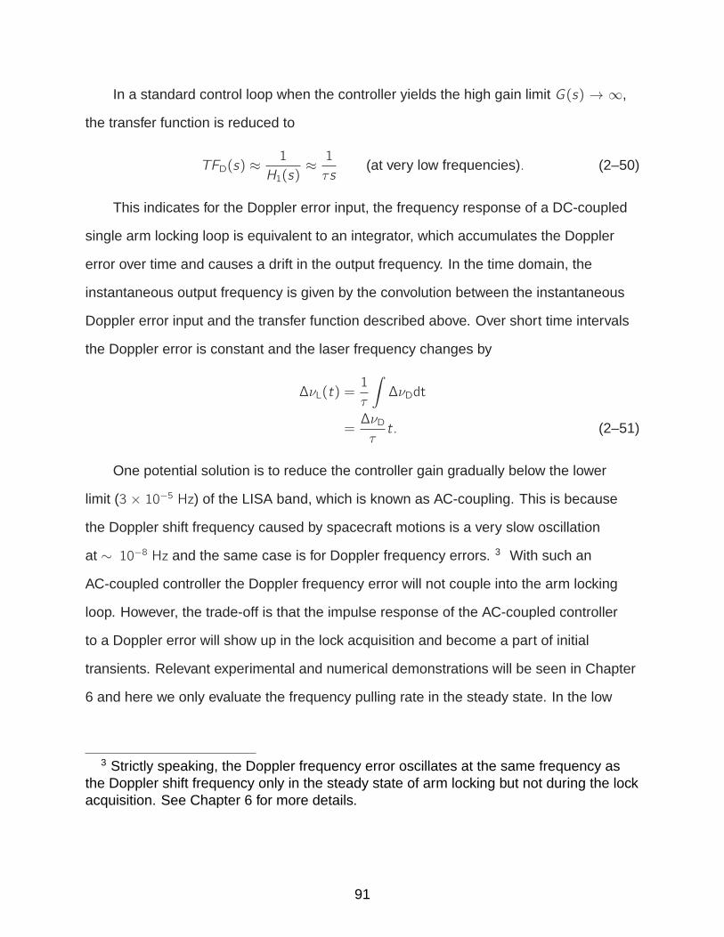
In a standard control loop when the controller yields the high gain limit G(s) → ∞,
the transfer function is reduced to
TFD(s) ≈1
H1(s)≈ 1
τs(at very low frequencies). (2–50)
This indicates for the Doppler error input, the frequency response of a DC-coupled
single arm locking loop is equivalent to an integrator, which accumulates the Doppler
error over time and causes a drift in the output frequency. In the time domain, the
instantaneous output frequency is given by the convolution between the instantaneous
Doppler error input and the transfer function described above. Over short time intervals
the Doppler error is constant and the laser frequency changes by
∆νL(t) =1
τ
∫∆νDdt
=∆νDτt. (2–51)
One potential solution is to reduce the controller gain gradually below the lower
limit (3 × 10⁻⁵ Hz) of the LISA band, which is known as AC-coupling. This is because
the Doppler shift frequency caused by spacecraft motions is a very slow oscillation
at ∼ 10−8 Hz and the same case is for Doppler frequency errors. 3 With such an
AC-coupled controller the Doppler frequency error will not couple into the arm locking
loop. However, the trade-off is that the impulse response of the AC-coupled controller
to a Doppler error will show up in the lock acquisition and become a part of initial
transients. Relevant experimental and numerical demonstrations will be seen in Chapter
6 and here we only evaluate the frequency pulling rate in the steady state. In the low
3 Strictly speaking, the Doppler frequency error oscillates at the same frequency asthe Doppler shift frequency only in the steady state of arm locking but not during the lockacquisition. See Chapter 6 for more details.
91

Figure 2-20. A generic dual arm locking loop with Doppler frequency errors in theLaplace domain. Two independent Doppler frequency errors are generatedat two phasemeters on the local spacecraft. When the two phasemeasurements are added and subtracted in the dual arm locking sensor,the Doppler frequency errors are also added and subtracted. Thedifferential Doppler error will be accumulated by the integrator in thedifferential path.
gain limit (H(s)G(s)→ 0 at very low frequencies), we have
TFD(s) ≈ G(s) (at very low frequencies). (2–52)
This means in the low gain limit, the effect on output frequency noise is simply the
input Doppler error multiplied with the controller gain in the low frequency range. Thus,
in the presence of an AC-coupled controller the Doppler error will not be accumulated by
the controller and consequently the residual effect is no more than an insignificant offset
added to the output laser frequency 4 .
Figure 2-20 shows that in dual arm locking the two arms generate two independent
Doppler errors ∆νD2 and ∆νD3, which can be combined to construct a common and a
4 The residual effect depends on the specific magnitude response of G(s) at very lowfrequencies. Here for simplicity we assume that G(s) provides a constantly low gaindown to DC.
92

differential Doppler error. We define
∆νD+ = ∆νD2 + ∆νD3,
∆νD− = ∆νD2 − ∆νD3. (2–53)
They will show up in the common and differential arm sensors independently and
will be amplified by the closed-loop gain in each path:
TFD+(s) =G(s)
1 + HD(s)G(s), (2–54)
TFD−(s) =G(s)E(s)
∆τs[1 + HD(s)G(s)]. (2–55)
In the common arm, TFD+(s) is approximately equal to 1/HD(s) in the high gain
limit. Since the magnitude of the dual arm locking sensor is flat at low frequencies,
a common Doppler error will only cause a frequency offset in dual arm locking. This
characteristics is to be distinguished from the frequency response of a common arm
locking loop to a common Doppler error. In that case the arm locking sensor is replaced
with H+(s) = P+(s). Consequently, in the high gain limit a common Doppler error
∆νD+ = ∆νD2 + ∆νD3 will cause the frequency pulling with a drift rate of ∆νD+/2τ .
In the differential arm, we have E(s) ≈ 1 and HD(s) ≈ 2 at low frequencies
and in the high gain limit the equation approaches 1/2∆τs . This frequency response
corresponds to a frequency drift rate given by
(dνLdt
)
D
=∆νD−2∆τ
. (2–56)
Since this drift rate is inversely proportional to the differential delay time, it
becomes undesirable when the arm length mismatch is very small, which is one of
the main disadvantages of dual arm locking. To reduce this frequency pulling, several
modifications to the controller have been proposed, including adding high-pass filters to
suppress the controller gain below the LISA band.
93

2.3.3.3 Modified dual arm locking
Modified dual arm locking was proposed by our group and, independently, by Kirk
McKenzie to solve the Doppler-induced frequency pulling problem as well as to enhance
the noise suppression performance [13]. The concept of modified dual arm locking is
to maintain the gain advantages of dual arm locking and recover the frequency pulling
characteristics of common arm locking by amplifying the common arm sensor below 1/τ
and keeping the dual arm sensor above 1/τ . This combination retains the overall flat
transfer function of the dual arm locking sensor below 1/2∆τ and significantly reduces
the frequency pulling due to a Doppler error.
The modified dual arm locking sensor is constructed based on a linear combination
of common arm locking sensor and dual arm locking sensor:
HMD(s) = FC(s)P+(s) + FD(s)HD(s), (2–57)
where FC(s) and FD(s) are two filters designed in a manner that the common arm
sensor dominates at frequencies below 1/∆τ and the dual arm locking sensor gradually
dominates above it. Although the design of FC(s) and FD(s) is not unique, FC(s) is
essentially a low-pass filter with one pole at DC and FD(s) is a high-pass filter with
a corner frequency around τ . Both filters require an appropriate gain to smooth the
crossover between the two sensors. An example of the specific design of FC(s) and
FD(s) is provided by Kirk McKenzie. The low-pass filter FC(s) has a pole at DC and a
lead compensator with a zero at 5/13τ and a pole at 5/2τ . The high-pass filter FD(s)
has four zeroes at DC, two poles at 7/10πτ , 11/20πτ and two poles at 1/90πτ . Here
we provide another relatively simpler design for our hardware simulations (See Section
5.3 for more details). The transfer function of our modified dual arm locking sensor is
illustrated in Figure 2-21, where both the magnitude response and the phase shift are
maintained in the LISA band. We also plot the magnitude and phase response of the
dual and common components that constitute the modified dual arm locking sensor in
94

10−4
10−3
10−2
10−1
100
101
10−2
100
Frequency (Hz)
Mag
nitu
de
10−4
10−3
10−2
10−1
100
101
−100
−50
0
50
100
Frequency (Hz)
Pha
se s
hift
(deg
ree)
Figure 2-21. The magnitude and phase response of the modified dual arm lockingsensor. The averaged light travel time is 33 s and the arm length mismatchis ∼ 1%. The modified dual arm locking sensor retains the flatness of thedual arm locking sensor transfer function. At frequencies near1/τ = 30 mHz the transfer function has some distortions coming from thecrossover between the common and dual arm components. (See Figure2-22)
Figure 2-22. The figure shows that the common arm component dominates frequencies
below 1/τ while the dual arm component dominates frequencies above it.
Eq. 2–57 can also be written as a linear combination of common arm sensor and
differential arm sensor:
HMD(s) = FC(s)P+(s) + FD(s)[P+(s) +E(s)
s∆τP−(s)]
= [FC(s) + FD(s)]P+(s) +E(s)FD(s)
s∆τP−(s)
= H+(s)P+(s) + H−(s)P−(s). (2–58)
It is easy to verify that the mapping vector of the modified dual arm locking sensor is
given by Sk(s) = [H++H−,H+−H−], where H+(s) = FC(s)+FD(s) and H−(s) =E(s)FD(s)s∆τ
.
Actually this general formalism can also be adapted to the common arm locking and
95
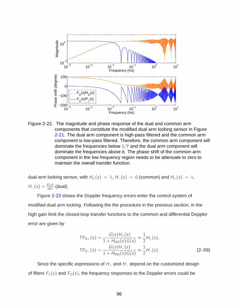
10−4
10−3
10−2
10−1
100
101
10−2
100
Frequency (Hz)
Mag
nitu
de
10−4
10−3
10−2
10−1
100
101
−200
−100
0
100
Frequency (Hz)
Pha
se s
hift
(deg
ree)
FD
(s)HD
(s)
FC
(s)P+(s)
Figure 2-22. The magnitude and phase response of the dual and common armcomponents that constitute the modified dual arm locking sensor in Figure2-21. The dual arm component is high-pass filtered and the common armcomponent is low-pass filtered. Therefore, the common arm component willdominate the frequencies below 1/τ and the dual arm component willdominate the frequencies above it. The phase shift of the common armcomponent in the low frequency region needs to be attenuate to zero tomaintain the overall transfer function.
dual arm locking sensor, with H+(s) = 1, H−(s) = 0 (common) and H+(s) = 1,
H−(s) =E(s)s∆τ
(dual).
Figure 2-23 shows the Doppler frequency errors enter the control system of
modified dual arm locking. Following the the procedure in the previous section, in the
high gain limit the closed-loop transfer functions to the common and differential Doppler
error are given by
TFD+(s) =G(s)H+(s)
1 + HMD(s)G(s)≈ 12H+(s),
TFD−(s) =G(s)H−(s)
1 + HMD(s)G(s)≈ 12H−(s). (2–59)
Since the specific expressions of H+ and H− depend on the customized design
of filters FC(s) and FD(s), the frequency responses to the Doppler errors could be
96

Figure 2-23. A generic modified dual arm locking loop with Doppler frequency errors inthe Laplace domain. Compared with Figure 2-20, two filters are placed inthe common and differential path individually. The high-pass filter in thedifferential arm path eliminates the frequency pulling due to the differentialDoppler error, while the low-pass filter design in the common arm pathallows the frequency pulling due to the common Doppler error. Note that itis also possible to high-pass filter the common arm path to eliminate thefrequency pulling completely, which is essentially equivalent to anAC-coupled controller.
complicated to calculate. However, as we know that essentially FC(s) is a low-pass filter
with one pole at DC and FD(s) is a high-pass filter with a corner frequency around 1/τ ,
the noise limitation can be roughly estimated using a simplified design of FC = 1s τ
and
FD =s
s+2π/τ. Thus we have
H+(s) =1
τs+
s
s + 2π/τ,
H−(s) =1
s∆τ
s
s + 2π/τ=1
∆τ
1
s + 2π/τ. (2–60)
We plot the magnitude responses of H+(s) and H−(s) with τ = 33 s and ∆τ = 0.16 s
in Figure 2-24. The magnitude responses of H+(s) and H−(s) feature a slope of 1/s τ
and 1/s∆τ , respectively. At low frequencies f ≪ 1/τ , H−(s) flattens out and approaches
a constant value of τ /(2π∆τ). At high frequencies f ≫ 1/τ , H+(s) flattens out and
approaches 1.
97
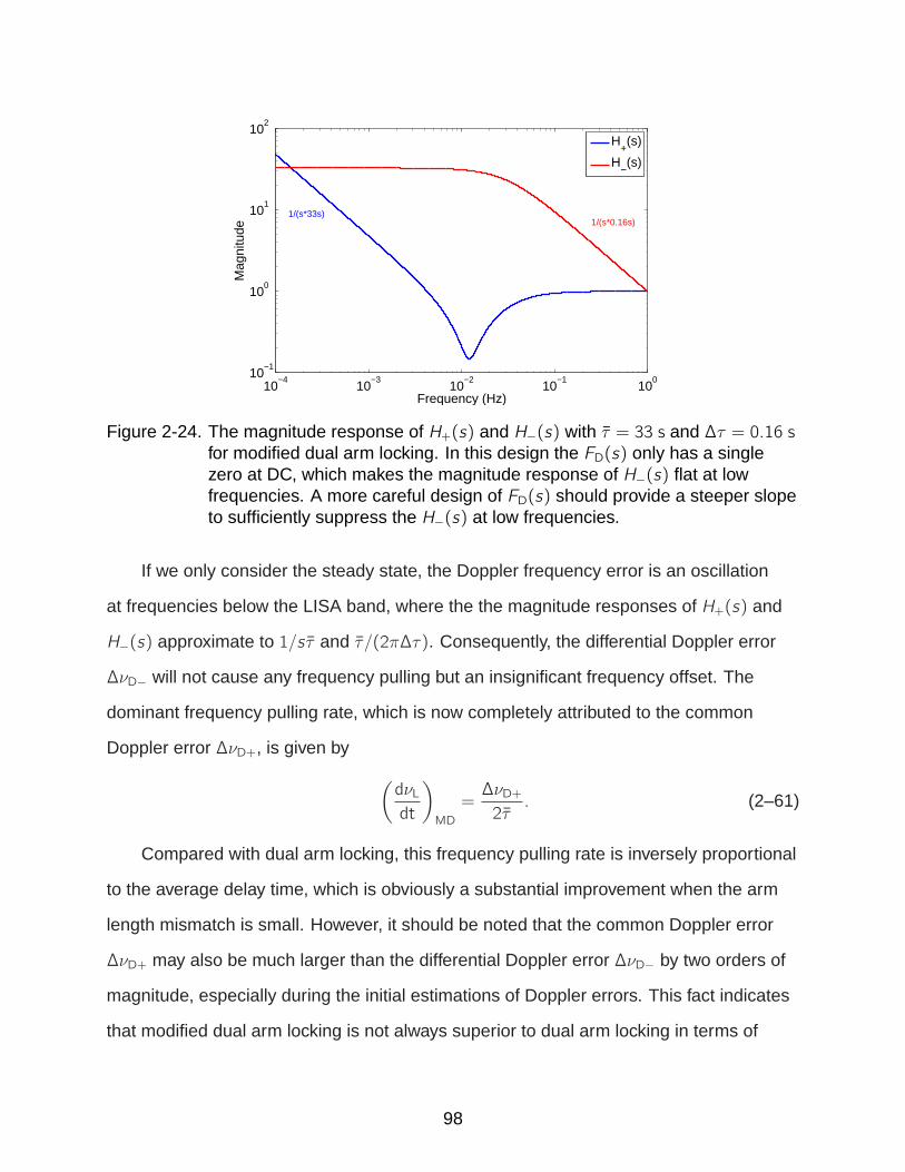
10−4
10−3
10−2
10−1
100
10−1
100
101
102
Frequency (Hz)
Mag
nitu
de
H+(s)
H−(s)
1/(s*0.16s)1/(s*33s)
Figure 2-24. The magnitude response of H+(s) and H−(s) with τ = 33 s and ∆τ = 0.16 sfor modified dual arm locking. In this design the FD(s) only has a singlezero at DC, which makes the magnitude response of H−(s) flat at lowfrequencies. A more careful design of FD(s) should provide a steeper slopeto sufficiently suppress the H−(s) at low frequencies.
If we only consider the steady state, the Doppler frequency error is an oscillation
at frequencies below the LISA band, where the the magnitude responses of H+(s) and
H−(s) approximate to 1/s τ and τ /(2π∆τ). Consequently, the differential Doppler error
∆νD− will not cause any frequency pulling but an insignificant frequency offset. The
dominant frequency pulling rate, which is now completely attributed to the common
Doppler error ∆νD+, is given by
(dνLdt
)
MD
=∆νD+2τ. (2–61)
Compared with dual arm locking, this frequency pulling rate is inversely proportional
to the average delay time, which is obviously a substantial improvement when the arm
length mismatch is small. However, it should be noted that the common Doppler error
∆νD+ may also be much larger than the differential Doppler error ∆νD− by two orders of
magnitude, especially during the initial estimations of Doppler errors. This fact indicates
that modified dual arm locking is not always superior to dual arm locking in terms of
98

frequency pulling. In realistic LISA, it should be allowed to switch to the proper arm
locking configuration between them according to the real-time arm length mismatch.
2.3.4 Integration with Tunable Pre-stabilization Referenc es
Before the frequency pulling caused by Doppler errors in arm locking was realized,
the integration of arm locking with pre-stabilization subsystems was already considered
because this combination would provide more noise suppressions to relax the
burden on TDI. The incorporation of arm locking with a pre-stabilization subsystem
requires the reference to be tunable because the lock points for the local reference
and the arm locking reference are not generally the same. For instance, a standard
Pound-Drever-Hall setup does not provide tunability between two resonant frequencies
of the reference cavity; therefore, some modification to the PDH setup must be present
to make the resonant frequency adjustable. Now the discovery of frequency pulling
increases the required tuning range for the local reference. A reasonable tuning range
of the reference should be well larger than the expected frequency pulling range of the
laser to avoid possible pre-stabilization issues. Given a cavity pre-stabilized laser and
200 s averaging estimation time, the frequency pulling on the stabilized laser is on the
level of a few MHz, which means the tuning range of the tunable reference should be at
least at tens of MHz.
Several tunability options with a sufficient tuning range have been suggested
for arm locking with different pre-stabilization schemes. Here we will discuss three
feasible options: Arm locking with Pound-Drever-Hall stabilization, arm locking with
Mach-Zehnder stabilization and arm locking without any pre-stabilization.
2.3.4.1 Arm locking with Pound-Drever-Hall stabilization
For Pound-Drever-Hall stabilization a simple approach is to replace the fixed optical
cavity with a PZT tunable cavity, which is actuated by the arm locking feedback signal.
As shown in Figure 2-25, by tuning the length of the cavity the central frequency of
the stabilized laser can be tuned and further stabilized by the arm locking controller.
99
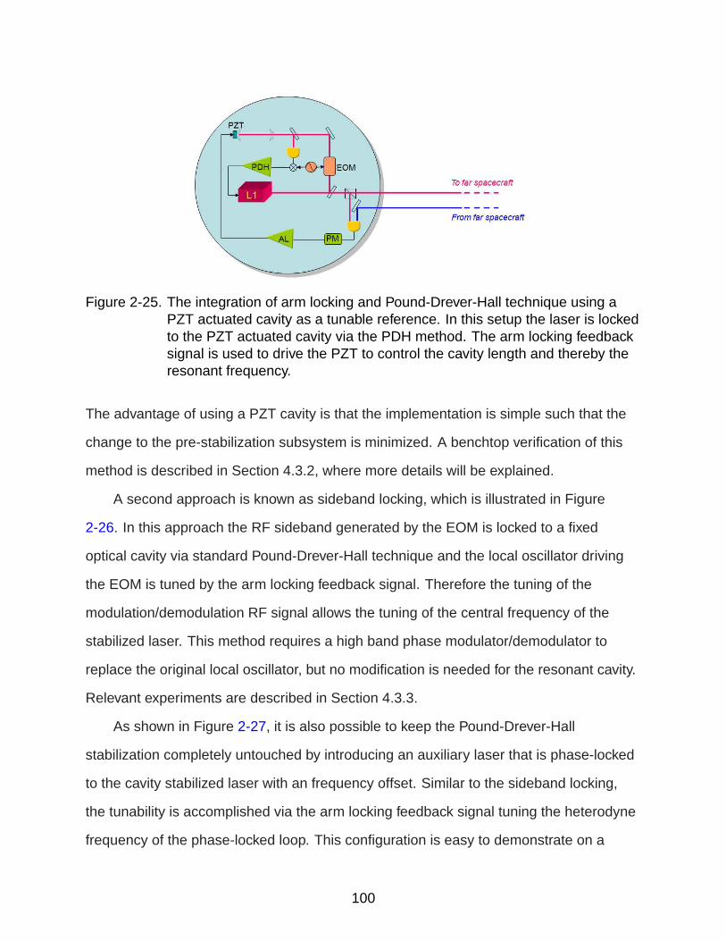
Figure 2-25. The integration of arm locking and Pound-Drever-Hall technique using aPZT actuated cavity as a tunable reference. In this setup the laser is lockedto the PZT actuated cavity via the PDH method. The arm locking feedbacksignal is used to drive the PZT to control the cavity length and thereby theresonant frequency.
The advantage of using a PZT cavity is that the implementation is simple such that the
change to the pre-stabilization subsystem is minimized. A benchtop verification of this
method is described in Section 4.3.2, where more details will be explained.
A second approach is known as sideband locking, which is illustrated in Figure
2-26. In this approach the RF sideband generated by the EOM is locked to a fixed
optical cavity via standard Pound-Drever-Hall technique and the local oscillator driving
the EOM is tuned by the arm locking feedback signal. Therefore the tuning of the
modulation/demodulation RF signal allows the tuning of the central frequency of the
stabilized laser. This method requires a high band phase modulator/demodulator to
replace the original local oscillator, but no modification is needed for the resonant cavity.
Relevant experiments are described in Section 4.3.3.
As shown in Figure 2-27, it is also possible to keep the Pound-Drever-Hall
stabilization completely untouched by introducing an auxiliary laser that is phase-locked
to the cavity stabilized laser with an frequency offset. Similar to the sideband locking,
the tunability is accomplished via the arm locking feedback signal tuning the heterodyne
frequency of the phase-locked loop. This configuration is easy to demonstrate on a
100

Figure 2-26. The integration of arm locking and Pound-Drever-Hall technique using afixed cavity locked to the sideband. In this setup the sideband frequency ofthe laser is locked to the fixed cavity via the PDH method. The arm lockingfeedback signal is used to adjust the modulation/demodulation RF signalthat drives the EOM.
Figure 2-27. The integration of arm locking and Pound-Drever-Hall technique using anauxiliary phase-locked laser. In this setup an auxiliary laser is heterodynephase-locked to the cavity stabilized laser. The arm locking feedback signalis used to adjust the local oscillator that drives the PLL.
benchtop but would require an additional laser in realistic LISA. The experimental
demonstration is described in Section 4.3.1.
It is also worth noting that in all these setups, the arm locking feedback signal is not
necessarily used to only adjust the actuators in the pre-stabilization setup; instead, it can
also be directly added to the feedback signal from the PDH controller to correct the laser
101

frequency. In practice, the arm locking feedback signal will be electronically split up and
enters the pre-stabilization loop at the two points described above; the laser frequency
therefore will be stabilized by their combination. The advantage of this configuration is
that the performance of the arm locking system is not limited by the bandwidth of the
pre-stabilization loop.
2.3.4.2 Arm locking with Mach-Zehnder stabilization
In addition to the standard Pound-Drever-Hall stabilization, the integration of arm
locking and other kinds of pre-stabilization subsystem has also been considered. In
particular we already mentioned the integration of arm locking with Mach-Zehnder
stabilization in Section 2.2.2.2. Unlike the widely discrete lock-points in the PDH
stabilization, Mach-Zehnder stabilization provides an inherent frequency tunability
described in Eq. 2–26, which makes the integration much simpler. In the integration the
arm locking feedback signal is not only used to adjust the phase of the local oscillator
that demodulates the heterodyne beat signal, but it is also directly added to the feedback
signal in the Mach-Zehnder stabilization. The second adjustment ensures that the
high-bandwidth arm locking performance can be retained and not affected by the low
bandwidth of the Mach-Zehnder setup. With the controller designed in Ref. [13], the
expected performance meets the TDI capability requirement with a margin greater than
50 at 1 Hz and 800 at 3 Hz.
2.3.4.3 Arm locking only
It is also possible to have arm locking take over the entire stabilization of the
laser frequency without any tunable pre-stabilization reference. In such an option
the arm locking feedback signal is directly sent back to the frequency actuator of the
laser controller; therefore the optical bench subsystem is totally untouched. Analytical
studies indicate that even without any pre-stabilization schemes, the dual/modified
dual arm locking will provide sufficient noise suppressions and meet the TDI capability
requirement across the entire LISA band in most time of a year [13]. The only period
102

Figure 2-28. Michelson-typed arm locking configuration with the phase-locked laser atthe far spacecraft.
when the arm locking performance is insufficient only lasts for 30 min, twice a year.
This happens when the arm length mismatch is less than 12 km. In the next section we
will analyze the noise limitations in arm locking and identify when they will become a
problem.
2.3.5 Arm Locking Limitations
In this section we consider the realistic limitations to the noise suppression
performance of arm locking. In reality, the stabilized laser frequency noise is dominated
by several expected noise sources. One of the nominal noise sources is the transponder
noise which comes from the phase-locking of the far laser. The transponder noise is
adequately removed in TDI algorithms; however, arm locking does not have any similar
mechanism to take care of it. We will analytically investigate how the transponder
noise will affect the arm locking performance. Also, the effects of other significant noise
sources, including noise of ultra-stable oscillators (USO’s), random spacecraft motion,
shot noise and technical noise will be discussed.
2.3.5.1 Limited controller gain in far-end PLL
Figure 2-28 illustrates the generic arm locking configuration with the incorporation of
the phase-locked laser at the far spacecraft, where the limited controller gain introduces
103

a transponder noise. In the analysis we first assume the far-end PLLs are closed
while the arm locking loop is still open. Based on Eq. 2–29, in the presence of a gain
limited far-end PLL, the phase measurement of the long arm interferometry at the local
spacecraft SC1 is given by
φ1i(s) = Φ0L1
(1− Gi
1 + Gie−sτi
)− 1
1 + GiΦ0Lie
−sτi1. (2–62)
The first term is directly related to the initial phase noise Φ0L1 of the pre-stabilized
local laser. The second term is an additional random noise source (the residual noise
unsuppressed by the far-end PLL) since Φ0L1 and Φ0Li are uncorrelated. Therefore, we
can still define the LISA arm transfer function, which yields the first term divided by the
the initial phase noise Φ0L1:
P1i(s) = 1−Gi
1 + Gie−sτi , (2–63)
which would be reduced to Eq. 2–30 when Gi ≫ 1. The definition of the arm locking
sensor H(s) remains the same as Eq. 2–33, but now it involves the PLL controller gain
Gi , i = 2, 3.
When the arm locking loop is closed, the stabilized phase noise of the local laser is
given by
ΦL1(s) = Φ0L1 −
G1
1 + G1HSk ·Φ1, (2–64)
where Sk is the mapping vector and Φ1 is a 2 × 1 phase vector describing the two
interferometer outputs. (See Section 2.3.1)
Now we calculate the stabilized phase noise depending on specific mapping vectors
individually. For single arm locking Sk = [1, 0], Eq 2–64 yields
ΦL1(s) = Φ0L1 −
G1
1 + G1H
(Φ0L1
(1− G2
1 + G2e−sτ2
)− 1
1 + G2Φ0L2e
−sτ21)
=1
1 + G1HΦ0L1 +
G1
1 + G1H
1
1 + G2Φ0L2e
−sτ21. (2–65)
104

The first term of Eq.2–65 demonstrates that the initial phase noise Φ0L1 is suppressed
by the open-loop gain G1H. The second term reflects the closed-loop response of
single arm locking to the transponder noise 11+G2Φ0L2. Essentially it is equivalent to a
Doppler frequency error introduced during the light travel as they both correspond to a
closed-loop response of G11+G1H
except for a trivial phase delay e−sτ21 . In the high gain
limit of the arm locking controller, the closed-loop response approximates to 1/H ≈ 1/τs ,
which increases the level of ΦL1(s) by the amount of the accumulated transponder
noise.
In the case of dual arm locking Sk = [1 +E(s)∆τs, 1 − E(s)
∆τs], if we use E(s) ≈ 1 in the
LISA frequency band, Eq 2–64 yields
ΦL1(s) = Φ0L1 −
G1
1 + G1H[1 +
1
∆τs, 1− 1
∆τs] ·
Φ0L1
(1− G2
1+G2e−sτ2
)− 11+G2Φ0L2e
−sτ21
Φ0L1
(1− G3
1+G3e−sτ3
)− 11+G3Φ0L3e
−sτ31
=1
1 + G1HΦ0L1 −
1
1 + G2Φ0L2e
−sτ21(1 +
1
∆τs
)− 1
1 + G3Φ0L3e
−sτ31(1 +
1
∆τs
).
(2–66)
The first term represents the idealized noise suppression. The additional effects of
the transponder noise, which are described by the other two terms, can be written as
δϕL1(s) =1
∆τs
(1
1 + G3Φ0L3e
−sτ31 − 1
1 + G2Φ0L2e
−sτ21)−(
1
1 + G3Φ0L3e
−sτ31 +1
1 + G2Φ0L2e
−sτ21).
(2–67)
The first term in Eq. 2–67 indicates that in the differential arm path the difference
between the transponder noises on two arms will be accumulated and scaled with 1/∆τ .
The second term indicates that in the common arm path the sum of the transponder
noises will be directly subtracted, which is negligible in comparison to the differential arm
path.
105
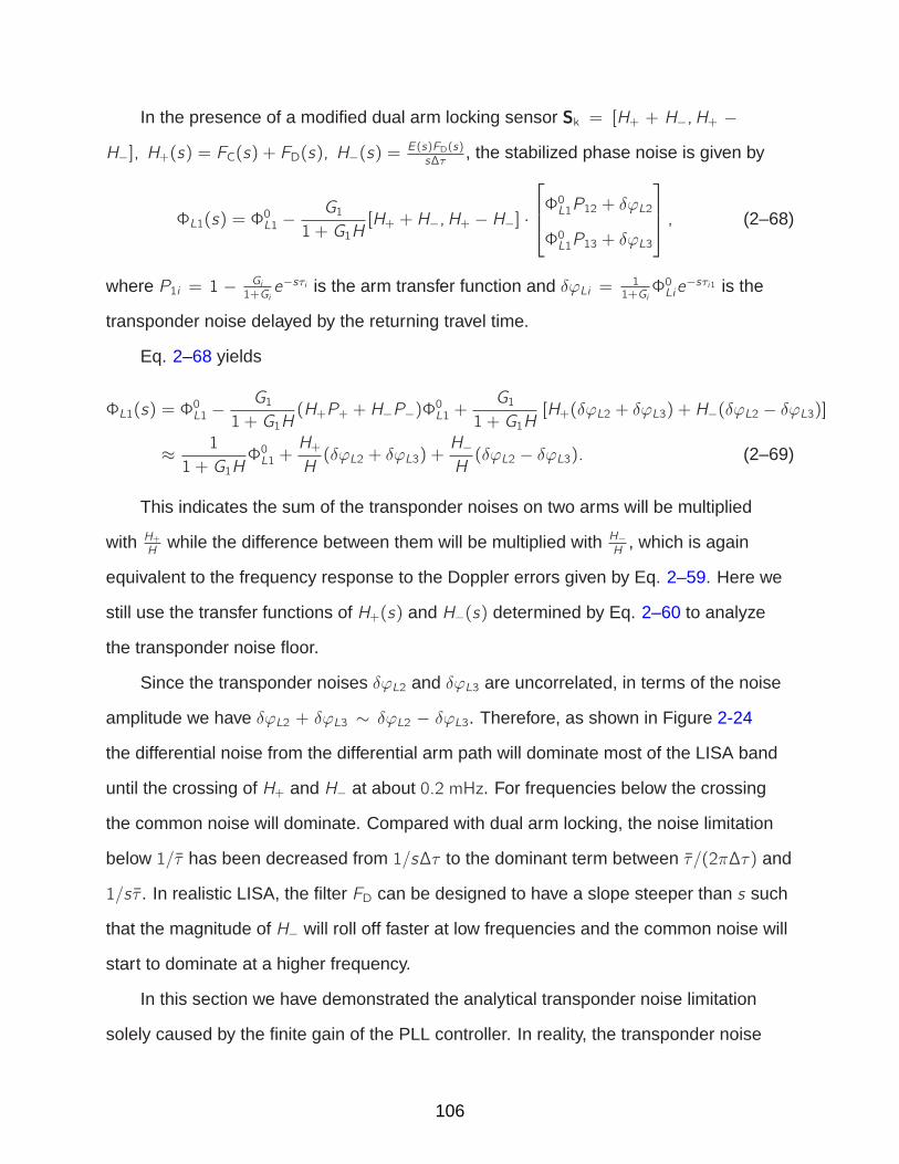
In the presence of a modified dual arm locking sensor Sk = [H+ + H−,H+ −
H−], H+(s) = FC(s) + FD(s), H−(s) =E(s)FD(s)s∆τ
, the stabilized phase noise is given by
ΦL1(s) = Φ0L1 −
G1
1 + G1H[H+ + H−,H+ − H−] ·
Φ0L1P12 + δϕL2
Φ0L1P13 + δϕL3
, (2–68)
where P1i = 1 − Gi1+Gie−sτi is the arm transfer function and δϕLi =
11+GiΦ0Lie
−sτi1 is the
transponder noise delayed by the returning travel time.
Eq. 2–68 yields
ΦL1(s) = Φ0L1 −
G1
1 + G1H(H+P+ + H−P−)Φ
0L1 +
G1
1 + G1H[H+(δϕL2 + δϕL3) + H−(δϕL2 − δϕL3)]
≈ 1
1 + G1HΦ0L1 +
H+
H(δϕL2 + δϕL3) +
H−H(δϕL2 − δϕL3). (2–69)
This indicates the sum of the transponder noises on two arms will be multiplied
with H+H
while the difference between them will be multiplied with H−
H, which is again
equivalent to the frequency response to the Doppler errors given by Eq. 2–59. Here we
still use the transfer functions of H+(s) and H−(s) determined by Eq. 2–60 to analyze
the transponder noise floor.
Since the transponder noises δϕL2 and δϕL3 are uncorrelated, in terms of the noise
amplitude we have δϕL2 + δϕL3 ∼ δϕL2 − δϕL3. Therefore, as shown in Figure 2-24
the differential noise from the differential arm path will dominate most of the LISA band
until the crossing of H+ and H− at about 0.2 mHz. For frequencies below the crossing
the common noise will dominate. Compared with dual arm locking, the noise limitation
below 1/τ has been decreased from 1/s∆τ to the dominant term between τ /(2π∆τ) and
1/s τ . In realistic LISA, the filter FD can be designed to have a slope steeper than s such
that the magnitude of H− will roll off faster at low frequencies and the common noise will
start to dominate at a higher frequency.
In this section we have demonstrated the analytical transponder noise limitation
solely caused by the finite gain of the PLL controller. In reality, the transponder noise
106

of the far-end PLL is primarily contributed other realistic noise sources, such as the
frequency noise that enters the ultra-stable oscillator driving the heterodyne PLL. The
frequency noise of the USO, or more frequently called clock noise, will also become a
part of the transponder noise and may further compromise the arm locking performance.
More details will be discussed in the next section.
2.3.5.2 Realistic noise sources in arm locking
The limitation of arm locking performance depends on several realistic noise
sources, as well as certain arm locking configurations that determine how the noise
sources will contribute to the stabilized laser frequency. Basically, the formalism used to
evaluate the effect of the transponder noise can be directly adapted to quantify the arm
locking limitation caused by these noise sources, only with different error points. So far,
significant noise sources that may be present in arm locking include:
• Clock noise - The phase of a beat signal is measured by comparing it to a timingreference (the local ultra-stable oscillator). Therefore, the acquired phase valueis always relative to the phase noise of the referencing clock. The clock noise isproportional to the nominal frequency Ω of the measured beat signal, i.e.,
δνclock(f ) = Ω · δν0clock(f ), (2–70)
where δν0clock(f ) are the fractional frequency fluctuations, corresponding to thenormalized clock frequency noise at 1 Hz clock frequency. The fractional frequencyfluctuation is estimated to be approximately 2.4 × 10⁻¹²/
√f Hz−1/2. The clock
noises from phasemeters on the same spacecraft are correlated, while they areuncorrelated on different spacecraft.
• Spacecraft motion - LISA arm length (benchtop to benchtop) is an excellentreference to stabilize the laser frequency. However, the stability of this lengthreference is still limited by the DRS that drags the spacecraft to track the geodesicmotion of the proof mass. The consequent length uncertainty is approximatelygiven by
δLSC(f ) = 2.5× 10⁻⁹√1 + (f /0.3 Hz)4 m Hz−1/2. (2–71)
The length uncertainty of one arm includes the spacecraft motions of twospacecraft at each end. This limited stability in the length reference will causea phase noise in the phase measurement.
• Shot noise - Limited number N of photons received per second by photodiodes.From Eq. 2–5, with 100pW light received at the photodiode the shot noise is given
107

Figure 2-29. The control system of arm locking with various noise sources entering theloop. In the diagram ϕC21 represents the clock noise introduced in thephase measurement of the beat signal φ21(t) = Φ2(t)−Φ1(t − τ12). Thesame notation is used for the shot noise ϕS and the phasemeter technicalnoise ϕT. ϕX21 represents the spacecraft motion of SC2 applied onto theinstantaneous phase Φ2(t) and the delayed phase Φ1(t − τ12).
by
δϕshot =1
2π√N=
√~c
2π
1
λP= 6.9× 10⁻⁶ cycles Hz−1/2. (2–72)
• Technical noise - Including the ADC noise in the A/D conversion of the beat signal,as well as the finite precision of integer arithmetic, known as the digitization noisein the phasemeters, arm locking sensor and controller. A digital signal with asampling frequency of fs and a precision of N-bit generally carries the digitizationnoise
δνdig =fclock · 2−N√6 · fs
. (2–73)
In the presence of a 50 MHz clock frequency and a 100 kHz data rate in a 48-bitphasemeter, the arm locking sensor will sense the digitization noise given by2.3× 10−10 Hz Hz−1/2.
Figure 2-29 illustrates the arm locking schematic including the realistic noise
sources described above. First we assume the far-end phase-locked loops are in
operation while the arm locking loop is not closed yet. Thus the laser phase noise
108

ΦLi , i = 2, 3 from the far spacecraft is given by
ΦLi(s) =1
1 + GiΦ0Li +
Gi
1 + Gi
(Φ0L1e
−sτ1i + ϕX1ie−sτ1i + ϕXi1 − ϕSi1 − ϕCi1 − ϕTi
). (2–74)
In this analysis we ignore the transponder noise 11+GiΦ0Li and assume the high gain
limit Gi1+Gi
≈ 1. Therefore, the phase noise of the long arm interferometry signal on the
local spacecraft is given by
φ1i(s) = Φ0L1(s)− (ΦLi(s) + ϕXi1) e
−sτi1 − ϕX1i + ϕS1i + ϕC1i + ϕT1i
≈ Φ0L1(s)P1i − ϕX1i(1 + e−sτi
)− 2ϕXi1e−sτi1
+ ϕSi1e−sτi1 + ϕS1i + ϕCi1e
−sτi1 + ϕC1i + ϕTie−sτi1 + ϕT1i. (2–75)
Following the notation used in Eq. 2–31, the phase noises of the two interferometer
outputs can be written together as a 2× 1 phase vector
Φ1(s) =
φ12(s)
φ13(s)
= [NL +NC +NX +NS +NT], (2–76)
where each vector is given by
NL =
Φ0L1(s)P12
Φ0L1(s)P13
, NC =
ϕC12 + ϕC21e
−sτ21
ϕC13 + ϕC31e−sτ31
, NT =
ϕT12 + ϕT2e
−sτ21
ϕT13 + ϕT3e−sτ31
NX =
−ϕX12 (1 + e
−sτ2)− 2ϕX21e−sτ21
−ϕX13 (1 + e−sτ3)− 2ϕX31e−sτ31
, NS =
ϕS12 + ϕS21e
−sτ21
ϕS13 + ϕS31e−sτ31
. (2–77)
Note that for NC, NX, NS and NT, each vector element consists of two noise terms
(e.g., ϕC12 and ϕC21) that come from two uncorrelated sources. The combined noise
amplitude is given by the quadrature sum of the two terms.
109

Table 2-1. Parameters of the noise analysis for arm locking
Parameter Symbol Value UnitsAverage delay time τ 33 sDifferential delay time ∆τ 0.016 sNominal frequency on arm 1-2 Ω12 15 MHzNominal frequency on arm 1-3 Ω13 −14 MHz
Fractional frequency fluctuation δν0clock 2.4× 10⁻¹²/√f Hz−1/2
Arm length stability (SC to SC) δLSC 2.5×√1 + (f /0.3 Hz)4 nm Hz−1/2
Received power at photodiodes P 100 pW
TDI capability δνTDI 282×√1 + (2.8 mHz/f )4 Hz Hz−1/2
Arm locking requirement [60] δνAL 0.3×√1 + (2.8 mHz/f )4 Hz Hz−1/2
When the arm locking loop is closed, we evaluate Eq. 2–64
ΦL1(s) = Φ0L1 −
G1
1 + G1HSk ·Φ1
=1
1 + G1HΦ0L1 −
G1
1 + G1HSk · [NC +NX +NS +NT]. (2–78)
The second term represents the noise limitations. Here we consider the arm locking
performance limited by various noise sources by assuming an infinite controller gain.
The analysis is based on the LISA parameters listed in Table 2-1 under different arm
locking configurations, where we neglect the technical noise as it should be small
compared to the other three. The arm length mismatch is assumed to be as short as
0.1%, corresponding to a 0.016 s differential time delay, in order to demonstrate a critical
scenario.
For common arm locking, the arm locking performance is independent of the arm
length mismatch. The noise limitations are plotted in Figure 2-30, which shows that for
frequencies above 20 mHz and below 0.7 mHz the common arm locking performance
is limited by spurious spacecraft motions and for frequencies in the middle range it is
dominated by the clock noise. At frequencies n/τ the spacecraft motion causse noise
peaks that may fail to meet the arm locking requirement.
For the dual arm locking configuration, the noise limitations are plotted in Figure
2-31. The dominant clock noise and spacecraft motion floor prevent arm locking from
110
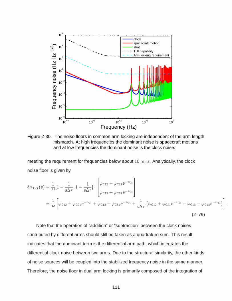
10−4
10−3
10−2
10−1
100
10−8
10−6
10−4
10−2
100
102
104
106
Frequency (Hz)
Fre
quen
cy n
oise
(H
z H
z−1/
2 )
clockspacecraft motionshotTDI capabilityArm locking requirement
Figure 2-30. The noise floors in common arm locking are independent of the arm lengthmismatch. At high frequencies the dominant noise is spacecraft motionsand at low frequencies the dominant noise is the clock noise.
meeting the requirement for frequencies below about 10 mHz. Analytically, the clock
noise floor is given by
δνclock(s) =1
H[1 +
1
s∆τ, 1− 1
s∆τ] ·
ϕC12 + ϕC21e
−sτ21
ϕC13 + ϕC31e−sτ31
=1
H
[ϕC12 + ϕC21e
−sτ21 + ϕC13 + ϕC31e−sτ31 +
1
s∆τ
(ϕC12 + ϕC21e
−sτ21 − ϕC13 − ϕC13e−sτ13)
].
(2–79)
Note that the operation of “addition” or “subtraction” between the clock noises
contributed by different arms should still be taken as a quadrature sum. This result
indicates that the dominant term is the differential arm path, which integrates the
differential clock noise between two arms. Due to the structural similarity, the other kinds
of noise sources will be coupled into the stabilized frequency noise in the same manner.
Therefore, the noise floor in dual arm locking is primarily composed of the integration of
111
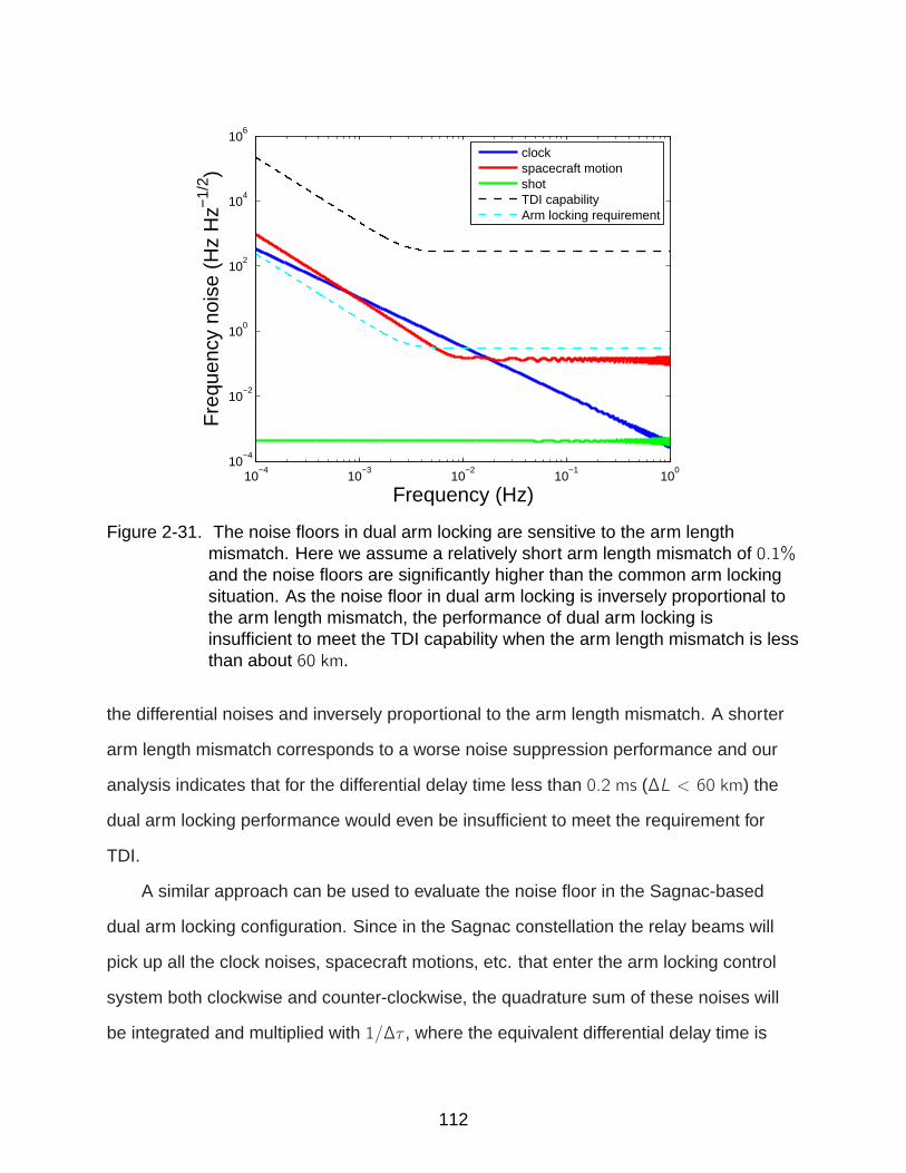
10−4
10−3
10−2
10−1
100
10−4
10−2
100
102
104
106
Frequency (Hz)
Fre
quen
cy n
oise
(H
z H
z−1/
2 )
clockspacecraft motionshotTDI capabilityArm locking requirement
Figure 2-31. The noise floors in dual arm locking are sensitive to the arm lengthmismatch. Here we assume a relatively short arm length mismatch of 0.1%and the noise floors are significantly higher than the common arm lockingsituation. As the noise floor in dual arm locking is inversely proportional tothe arm length mismatch, the performance of dual arm locking isinsufficient to meet the TDI capability when the arm length mismatch is lessthan about 60 km.
the differential noises and inversely proportional to the arm length mismatch. A shorter
arm length mismatch corresponds to a worse noise suppression performance and our
analysis indicates that for the differential delay time less than 0.2 ms (∆L < 60 km) the
dual arm locking performance would even be insufficient to meet the requirement for
TDI.
A similar approach can be used to evaluate the noise floor in the Sagnac-based
dual arm locking configuration. Since in the Sagnac constellation the relay beams will
pick up all the clock noises, spacecraft motions, etc. that enter the arm locking control
system both clockwise and counter-clockwise, the quadrature sum of these noises will
be integrated and multiplied with 1/∆τ , where the equivalent differential delay time is
112

10−4
10−3
10−2
10−1
100
10−6
10−4
10−2
100
102
104
106
Frequency (Hz)
Fre
quen
cy n
oise
(H
z H
z−1/
2 )
clockspacecraft motionshotTDI capabilityArm locking requirement
Figure 2-32. The noise floors in modified dual arm locking are less dependent on thearm length mismatch due to the low-frequency filtering scheme. The noisefloors are effectively suppressed by the high-pass filter at frequenciesbelow 1/τ . With a more carefully designed high-pass filter, the noise floorswill be further reduced and asymptotically approach the noise floorsdetermined in the common arm locking configuration.
≈ 47 µs. Since every noise source will contribute to the overall noise floor twice and
scale with a very short differential delay, the noise limitation in Sagnac-based dual arm
locking is much higher than any other arm locking configuration.
The analysis for modified dual arm locking can be adapted from Eq. 2–69. For the
modified dual arm locking sensor [H+ + H−,H+ − H−], the clock noise floor is given by
δνclock(s) =H+
H(ϕC12+ϕC21e
−sτ21+ϕC13+ϕC31e−sτ31)+
H−H(ϕC12+ϕC21e
−sτ21−ϕC13−ϕC31e−sτ31).
(2–80)
As a simple demonstration, we still take H+(s) and H−(s) given by Eq. 2–60 as
an example. The noise limitations are plotted in Figure 2-32. Compared with the noise
limitation in dual arm locking, the noise level has been decreased below the arm locking
113

requirement for the entire LISA band, which is well below the TDI capability. Note that
due to the simplified design of FD(s), which exhibits an unoptimized s slope, the noise
floors at low frequencies are not maximally suppressed. In realistic LISA a better noise
suppression performance should be expected with a more carefully designed FD(s)
if modified dual arm locking will be used. If the magnitude of the FD(s) filter rolls off
faster at low frequencies, the noise floors will become less dependent on the arm length
mismatch and asymptotically approach the floor determined by 1/τ .
At the end of this chapter let us have a brief estimation regarding the LISA
arm length mismatch. Now that we know a short arm length mismatch is critical for
Doppler-induced frequency pulling and the arm locking performance, we are interested
in how long a critical scenario, say |∆L/L| < 0.1%, will last in the orbital period of one
year. As we know, the arm length mismatch is roughly a sinusoid function with a period
of one year and the maximum mismatch is about 1%, i.e.,
∆L = 0.01× L · sinΩt, (2–81)
where Ω = 2π/1 yr ≈ 2× 10⁻⁷ Hz.
Therefore, the arm length mismatch is
∆L ≈ 5× 10⁷ m · sin(2× 10⁻⁷ Hz · t) ≈ 10 m s−1 · t. (2–82)
Thus we obtain the change rate of arm length mismatch of approximately 10 m s−1.
For the arm length mismatch below ±0.1%, the duration is approximately 2 × 5 ×
106 m/10 m s−1 ≈ 106 s, which is less than 12 days, twice per year. Note that this is just
a quick and rough estimation and a more deliberate calculation depends on the exact
LISA orbits. Nevertheless, it still gives us the information that the performance of arm
locking will not be substantially degraded by the arm length variations and the scenario
will only become critical during a short amount of time every year.
114
CHAPTER 3UNIVERSITY OF FLORIDA LISA INTERFEROMETER SIMULATOR
The LISA group at the University of Florida has developed a hardware in the
loop simulator for LISA’s long arm interferometry which is similar to LISA as possible.
So far, a synthesized hardware LISA interferometry and measurement system, the
University of Florida LISA Interferometer Simulator (UFLIS), which consists of a variety
of LISA component models, has been developed with continuous modification and
enhancement. These component models include LISA-like cavity pre-stabilization,
digital integrated-circuit board based science phasemeters, LISA-like inter-SC ranging
and laser communications, LISA-like variable light travel time and variable Doppler
shifts, analog/digital hybrid realistic arm locking, synthesized realistic TDI with fractional
delay filtering, generation of gravitational-wave-like signals, etc.
UFLIS is currently the only existing hardware system that can realistically simulate
long arm interferometry by providing LISA-like light travel time as well as variable
Doppler shifts. Since the three interferometers are independent to each other in
the IMS, the absence of the other two interferometer will not degrade the validity
of our experiments but will also the reduce the complexity. A long-term goal of
UFLIS is to inject the generated gravitational-wave-like signals into the simulator
and mock the LISA data within the required noise level, and to successfully extract the
gravitational-wave-like signals by developing proper LISA data analysis methods. In
this chapter we will introduce the current research on the optical/electronic components
related to the hardware simulation of arm locking, which are accomplished by our group
at the University of Florida.
3.1 Optical Components
In the current optical layout of LISA interferometry benchtop, three 1064 nm Nd:YAG
lasers are referred to as Li , i = 1, 2, 3, respectively. Another independent Nd:YAG laser
RL is a reference laser which functions as an optical clock to generate beat signals
115

10−4
10−2
100
100
101
102
103
104
105
106
Frequency (Hz)
Fre
quen
cy n
oise
(H
z/rt
Hz)
RL − L1 beat signalTDI capability
Figure 3-1. Frequency noise of the beat signal between two cavity stabilized laser RLand L1.
with frequencies below 20MHz with each of the other three lasers. The reason we use
beat signal rather than the direct laser frequency is that a single laser frequency is in
the range of 300 THz which is not possible to be measured by a normal commercial
photodiode.
The lasers RL and L1 are separately locked to their own reference high finesse
optical cavity using Pound-Drever-Hall technique for pre-stabilization. Each cavity
consists of a Zerodur spacer. Therefore, the beat signal between RL and L1 provides
the input phase noise on the master spacecraft in TDI and arm locking setup. The beat
signals between RL and L2 or L3 can be used as returning beams from far spacecraft
with L2 or L3 phase-locked to the master laser L1.
Figure 3-1 shows the frequency noise spectrum of the beat signal between RL
and L1 at a nominal frequency of approximately 13 MHz. In the frequency range from
1 mHz to 1 Hz, the frequency noise stays at a level of approximately 100 ∼ 200 Hz/√Hz,
which is already below the 282 Hz Hz−1/2 pre-TDI frequency noise requirement. Also,
the beat frequency exhibits a long term linear drift by up to ±1 MHz, with a typical drift
116

rate of 1 Hz/s. This moderate frequency drift can be taken out in the data processing
and essentially has no significant influence on laser measurements.
3.2 Electronic Components
To reproduce the measurement environment in LISA’s long arm interferometry,
we selected a high-speed digital signal processing system (referred to as the “Pentek
board”) manufactured by the Pentek Corporation. Phasemeters, as well as most
important electronic components of UFLIS, are all implemented on this system.
3.2.1 Digital Signal Processing Hardware
The Pentek board consists of three individual electronic boards: Model 4205
motherboard, Model 6256 A/D daughterboard and Model 6228 D/A daughterboard.
Model 4205 contains the following primary elements:
• A 32-bit central microprocessor (CPU) with a 1 GHz clock frequency: Like allCPUs, it carries out each instruction of the program in sequence and performs thebasic arithmetical, logical, and input/output operations of the system.
• A 1 GB synchronous dynamic random access memory (SDRAM): It is used tostore data while synchronized with the system’s PCI bus (meaning it waits for aclock signal before responding to control inputs).
• Four 32-bit velocity interface modules (VIMs): VIM is an interface for the datatransfer and communications between the motherboard and the daughterboards.Each two VIMs are connected to one daughterboard, with one data interface andone control/status interface.
• Four bi-directional first-in first-out buffers (BIFOs): After/Before the data istransfered through the VIM, the data will first be written into the BIFO beforememory access. Each BIFO is connected to one VIM. Data transfer can also berealized directly between different VIMs without the process of writing/reading intothe memory.
• Four direct memory access (DMA) controllers: DMA is capable of reading/writingdata from/into the BIFO while directly accessing the memory for reading andwriting independently of the intervention from the CPU.
• One serial and one Ethernet port: These ports are for the communication betweenModel 4205 and computers to upload/download commands and files.
117

The Model 6256 A/D daughterboard and the Model 6228 D/A daughterboard are
connected to the Model 4205 motherboard via VIMs. The primary elements on Model
6256 include:
• Four 14-bit analog-digital converters (ADCs): These ADCs can be clocked at up to105 MHz. Since the connectors of these ADCs are AC-coupled with a high-passfilter, the ADCs can only digitize an RF signal with the carrier frequency higherthan 400 kHz, which is ideal for LISA-like heterodyne beat signals. The full scale ofthe ADC input amplitude is 4 dBm.
• Two Xilinx Virtex-2 field programmable gate arrays (FPGAs): The digital signalfrom the ADCs will be sent to the FPGAs, where the logical functions andoperations in digital signal processing can be implemented. FPGA containsprogrammable logic components known as logic blocks, and a hierarchy ofreconfigurable interconnects that allow the blocks to be wired together, whichallows us to easily configure the FPGA according to the required design. Thedigital signal on the FPGA yields fixed-point arithmetic, which limits the dataprecision while improves the calculation efficiency.
The primary elements on Model 6228 include:
• Four 16-bit digital-analog converters (DACs): These DACs can be clocked at up to500 MHz. Similar to the ADCs, the DACs are also AC-coupled such that they canonly generate RF signals with the carrier frequency higher than 400 kHz. The fullscale of the DAC output amplitude is −2 dBm.
• A Xilinx Virtex-2 field programmable gate array (FPGA): Model 6228 also providesa similar FPGA that can be programmed for signal processing. The FPGA can bedirectly connected to the inputs of the DACs.
With these three models, the Pentek board can realize a variety of functions such
as the data acquisition, signal measurement and digital filtering. In the following sections
we will discuss two basic applications of the Pentek board, which have been widely used
in UFLIS.
3.2.2 Phasemeter
Phasemeter is the most fundamental instrument in LISA’s measurement system.
It is essential for the precise measurement of heterodyne interferometry phases
at photodiodes, which is the primary quantities to be measured in IMS. Moreover,
phasemeters play an important role in digital control loops in which the sensor detects
118

Figure 3-2. The implementation of the phasemeter on a Pentek board. The phasemeteris essentially a “frequency meter” that tracks the frequency fluctuations ofthe input signal.
the phase, e.g., phase-locking and arm-locking. Therefore, phasemeters can be
classified into two types based on the different functions. The former type focuses
on the phase measurement in the LISA band, requiring high precisions with a low data
rate (∼ 3 Hz). The latter type focuses on the phase detection in digital controls where a
high bandwidth and consequently fast data rate (∼ 100 kHz) will be needed.
As discussed in Section 2.3.5, the phase is measured with respect to a clock
reference such that the acquired phase value is always relative to the phase noise of the
referencing clock. Therefore, all phase measurements inevitably carry the clock noise.
3.2.2.1 Design
Given that the desired sensitivity of IMS is approximately 18 pm/√Hz, the science
phasemeter needs to be able to measure the arm length change with a precision of
∼ 1 pm/√Hz. Therefore, the phase measurement with 1064 nm wavelength is required
to have an accuracy of ∼ 1µcycles/√Hz [59].
The phasemeter developed at the University of Florida adapts an architecture
of digital phase-locking similar to the LISA phasemeter. As shown in Figure 3-2, the
phasemeter is implemented on the Model 6256 A/D daughterboard. The clock frequency
119

to operate the 14-bit ADC is fclock = 62.5 MHz. The digitized heterodyne signal, which
carries a frequency ν0 + δν(t) is demodulated by a 48-bit numerical control oscillator
(NCO) that is phase-locked to the measured signal. The NCO frequency νm tracks
the frequency of the measured signal, and it is given by the sum of a 16-bit preset
offset frequency νoff and a 48-bit time-varying frequency correction νcorr. The frequency
difference between the NCO and the measured signal gives the PLL error νe. Based on
the phasemeter model shown in Figure 3-2, we have
νcorr = νe · G ,
νm = νoff + νcorr,
νe = ν0 + δν(t)− νm, (3–1)
where G is the transfer function of the PLL controller satisfying the condition G ≫ 1. We
solve νcorr given by
νcorr =G
1 + G[δν(t) + (ν0 − νoff)] ≈ δν(t) + (ν0 − νoff). (3–2)
Therefore, the frequency fluctuations of the measured signal is faithfully reproduced
by νcorr if ν0 = νoff within the phasemeter bandwidth. If the preset offset frequency is
not exactly equal to ν0, a constant offset will be added into νcorr. This frequency offset
can be easily removed in post-processing of phase measurements, but might cause a
frequency pulling issue in arm locking.
The phasemeter is essentially a “frequency meter” that detects the frequency
fluctuations of the beat signal. Integrating the frequency fluctuations will generate the
phase information: δϕ(t) =∫ t0δν(t)dt. This integration can be done in post-processing.
Note that the phase measurement can also be achieved by integrating the NCO
frequency νm. As the NCO frequency contains the constant frequency offset, a linear
drift in phase will show up in the result.
120

10−4
10−3
10−2
10−1
100
10−8
10−6
10−4
10−2
100
102
104
Frequency (Hz)
Pha
se n
oise
(cy
cle/
rtH
z)
Chan 1Chan 2Residual1 pm requirement
Figure 3-3. The phasemeter performance measured with split-and-subtracted VCOsignals. The noise limitation of the phasemeter is the ADC noise, which iscontributed by the temperature fluctuations for low RF frequencies andtiming jitter for high RF frequencies. Although the ADC noise floor preventsthe phasemeter from meeting the 1 pm requirement, it does not cause asignificant problem in our arm locking experiments. However, the noisesuppression performance in our tests may be limited by the ADC noise,which will be seen in Chapter 5.
The main loop of the digital PLL is running at fclock/128 ≈ 488 kHz as downsampled
by a cascaded integrating comb (CIC) filter with a factor of 128. The data rate of the
frequency fluctuations can be further downsampled to 61.0 kHz or 14.9 Hz, depending
on whether the function of the phasemeter data is high-bandwidth tracking or science
measurements. However, in our arm locking setup we directly use the 488 kHz
frequency data stream without any additional downsampling stage to minimize the
system processing delay (see the next chapter).
3.2.2.2 Performance
The phasemeter is characterized by taking measurements of a voltage controlled
oscillator (VCO) signal, as shown in Figure 3-3. In this simple setup, the 4 MHz VCO
signal is split by an electronic splitter and measured by two phasemeters. The two
phasemeters are programmed on the same FPGA but connected to different ADCs;
121
therefore, they have a common clock noise but uncorrelated ADC noises. Figure 3-3
shows that the noise spectrum of their difference is limited by a 1/√f ADC noise floor,
which is empirically given by
ϕADC(f ) =3× 10⁻⁷√
f· ν04 MHz
cycle Hz−1/2, (3–3)
where ν0 is the nominal frequency of the input signal.
In addition, the finite precision of the fixed integers in the phasemeter causes the
digitization noise as frequency noise given by
νDig(f ) =fclock · 2−N√6 · fs
, (3–4)
which is a limited-bandwidth white noise in terms of frequency fluctuations. For the high
sampling frequency of 61.0 kHz, the digitization noise of the 48-bit phasemeter is about
3.67× 10⁻¹⁰ Hz Hz−1/2. For the low sampling frequency of 14.9 Hz, the digitization noise
is about 2.35 × 10⁻⁸ Hz Hz−1/2. When converted into phase fluctuations, the digitization
noise floor is marginally below the 1 pm requirement curve.
Latest progress on the phasemeter development indicates that the ADC noise
source is primarily attributed to the tempature-dependent phase dispersion in the RF
transformer for low RF frequencies (< 8 MHz) and timing jitter for high RF frequencies
(> 8 MHz). The phasemeter sensitivity performance has been substantially improved
by replacing the RF transformers and has already met the 1 pm Hz−1/2 requirement.
Nevertheless, it should be noted that the phasemeters used in current EPD units (see
the next section) and arm locking setup described in this dissertation have not adapted
this enhancement.
3.2.3 Electronic Phase Delay
A challenging issue in benchtop experiments of LISA interferometry is the
simulation of the round-trip propagation between spacecraft. The difficulty of reproducing
a LISA-like 33 s delay line compromises the validity of LISA interferometry experiments
122

of TDI or arm locking. Compared with unrealistic short delay lines via very long cables
or fibers used in most laboratories [89, 90], one distinctive feature of UFLIS is the
emulation of realistic LISA-like delay times and MHz-range Doppler shifts via electronic
delay. Such an electronic delay system built with high-bandwidth phasemeters is called
an Electronic Phase Delay (EPD) unit.
The EPD system is also implemented on a Pentek board [91, 92] clocked at
62.5 MHz. An EPD unit consists of three main components, which are implemented
on three parts of the Pentek board respectively. The Model 6256 A/D daughtercard is
programmed with a 48-bit phasemeter. 1 The phasemeter measures the frequency
fluctuation of the digitized laser beat note with a data rate of 61 kHz and then send the
data stream to the memory of the Model 4205 motherboard. The motherboard stores
the frequency information in a memory buffer for a certain amount of time. The high
data rate in the phasemeter ensures the frequency information within the arm locking
bandwidth (∼ kHz) can be properly delayed by the EPD system. After the delay in the
memory buffer, the frequency information is sent to the Model 6228 D/A daughtercard,
where an NCO integrates the sum of the frequency fluctuation and the frequency
offset to regenerate the delayed copy of the input laser phase. After the NCO output,
the digitized signal is converted back to an analog signal by the 500 MHz sampling
frequency D/A converter. During this routine, a MHz-range Doppler frequency can be
added dynamically to the nominal frequency of the delayed signal on the motherboard.
The EPD unit is capable of delaying a MHz-range signal by as long as 280 s. The
performance of the EPD unit is measured using a simple setup where the VCO signal is
electronically split and one channel is delayed by 1 s through the EPD unit. We measure
1 Actually, the FPGA is programmed with four identical phasemeters that areconnected to four different ADCs in order to operate four-channel delays simultaneously.Here we just consider a one-channel case for the purpose of simplicity.
123

10−3
10−2
10−1
100
101
10−2
10−1
100
Frequency (Hz)
Mag
nitu
de
idealizedmeasured
10−3
10−2
10−1
100
101
10−5
100
105
Frequency (Hz)
Pha
se n
oise
(cy
cles
/rtH
z)
Linear Spectral Density
Prompt phaseDelay phaseDifferential phase (fractional delayed)
Figure 3-4. (Left) The magnitude response of an interferometer response with 1 s delay.(Right) The phase noise spectrum of the EPD unit.
the frequency/phase noise of the delayed signal and the prompt signal individually. The
interferometer response of a LISA arm, which also yields a single arm locking sensor, is
given by
P12(s) = 1− e−sτ =φ12(s)
φ0(s), (3–5)
where φ12(s) is the difference φ0(t)− φ0(t − τ) between channel 1 and 2 represented in
the Laplace domain.
The measurement results are shown in Figure 3-4. The left figure shows the
magnitude response of P12(s), which exhibits interferometer nulls at n/τ and an s slope
for frequencies far below 1/τ . The right figure shows the noise floor of the EPD unit. To
evaluate the additional noise induced by the EPD unit, we time shift and fractional delay
filter the delayed phase such that its time series could be maximally synchronized to
the prompt phase in post-processing. Thus the EPD noise is given by differential phase
noise between the two signals. The measured EPD noise is essentially on an equivalent
level as the ADC noise in the phasemeter, since the primary contribution to the EPD
noise is from the phasemeter ADCs. Note that the apparent increment of the EPD noise
at frequencies above 1 Hz shown in the figure is an artifact from fractional delay filtering,
while in reality the EPD noise continues to decrease with the same trend.
124

CHAPTER 4EXPERIMENTAL VERIFICATION OF SINGLE ARM LOCKING
4.1 Motivation
Currently, UFLIS is the only existing hardware system that can simulate arm locking
experimentally under realistic conditions, which is mainly ascribed to the long light travel
time provided by the EPD unit. Compared with previous single arm locking experiments
which were limited to µs delay times produced by long cables [89] or fibers, the first
generation of EPD-based arm locking hardware simulations by Ira Thorpe has achieved
significant progress [93]. Nevertheless, the first generation arm locking on UFLIS is still
an extremely simplified model as it exploited only one single arm to build the sensor
and did not add the Doppler shift as well as the noise limitations into the setup. By
summarizing the discussions in Section 2.3, we list the following conditions that need to
be reflected in a realistic arm locking hardware simulation.
• Due to the significant advantages of dual/modified dual arm locking, the errorsignal of arm locking has to be a combination of two interferometry signals, whichmeans we need to have two delay lines, two phasemeters and a mapping vectorimplemented on the hardware system.
• The round-trip time on each arm should be around 33 seconds and, if possible,time-dependent. The arm length mismatch should be generated in a realistic range(no more than ∼ 1%, but also not equal to zero).
• The phase noise introduced by the phase-locked controller on the far spacecraftwill couple into the sensor such that it cannot be suppressed by the arm lockingcontroller. Therefore, the PLL on the far-end should be implemented realisticallyrather than be assumed to have an infinite gain given by an ideal optical transponder.
• A Doppler shift frequency applied to the heterodyne frequency of the beat signalneeds to be taken into account. Also, a time-dependent Doppler shift frequency isdesirable.
• Because it is impractical to measure and update the Doppler frequency on everydata cycle, a Doppler frequency error within an acceptable range should beintroduced.
• Finally there are other important noise sources we need to consider, including theclock noise in the phase measurement, the spacecraft jitter and the shot noise at
125

photodiodes. These noise sources will limit the noise suppression performance.And the effect of gravitational waves on arm locking should also be considered inorder to investigate the impact of arm locking on gravitational wave detections.
The ultimate goal of arm locking simulations on UFLIS is to reproduce the above
conditions, suppress the laser frequency noise and incorporate it into a TDI experiment
to demonstrate the primary functions of IMS. A methodical procedure to build such
an ultimate arm locking hardware system is to start with the basic single arm locking
loop and take the realistic conditions into account stepwise. Thus in this chapter we will
describe a series of enhanced single arm locking experiments which feature Doppler
shifts [14] and incorporation with a tunable reference.
In our experimental verification of single arm locking, we use a MHz beat signal
between two cavity stabilized lasers as the input noise source. This provides a
frequency noise of approximately 100 − 200 Hz Hz−1/2 at frequencies above ∼ 1 mHz.
The single arm locking sensor, which is essentially the interferometer response of a
single arm, is an electronic model same as the transfer function in Figure 3-4. The
realistic round-trip travel time on the LISA arm is simulated via the EPD unit, where
variable Doppler frequency shifts can be added to the nominal frequency of the delay
signal. The arm locking controller is implemented on a second Pentek board, where a
phasemeter will first measure the error signal with a high data rate (∼ 488 kHz) and then
send the data to a feedback filter (Section 4.2.2). The feedback signal from the controller
output will be used to drive the actuator (a tunable frequency reference) to control
the laser frequency. The actuator can be either a PZT actuator to tune the resonant
frequency of the reference cavity (Section 4.3.2), or a local oscillator of a heterodyne
phase-locked loop (Section 4.3.1).
Among these components, the sensor transfer function determines the controller
design, because the slope of the controller filter will need to preserve some extra phase
for frequencies above the first null in the sensor. To simplify our experiment setup, we
set the delay time to be approximately 1 s at the EPD unit, which is still much longer
126

than the delay times used in previous arm locking experiments. The benefit is that in this
case we only need to be concerned with the filter design in the frequency range above
1 Hz. Also, the 1 s delay time is comparable to the typical differential delay time when
the second LISA arm is used to test the dual/modified dual arm locking configurations,
where the sensor nulls are located at or above a few Hz.
4.2 Preliminary Test With Numerical Control Oscillator (NCO) Tracking
Before we actually start to build a complete realistic arm locking system incorporated
with pre-stabilized lasers, it is reasonable to preliminarily verify the noise suppression
capability and closed-loop stability of a basic single arm locking loop. Such a basic
single arm locking loop does not need to be incorporated with a tunable reference,
but simply reflects the closed-loop dynamics of the feedback control system. Also, the
realistic noise limitations as well as Doppler frequency errors should be insignificant
enough such that they should only cause negligible effects on the measurement results.
A straightforward model to test a basic single arm locking loop is an electronic model
with a VCO signal or a laser beat signal between two cavity stabilized lasers as the input
noise.
4.2.1 Experimental Setup
The preliminary experimental setup is essentially a single arm locking loop featuring
the EPD unit to stabilize the frequency of a numerical control oscillator (NCO) to a
noisy laser beat signal. As shown in Figure 4-1, the NCO signal driven by the controller
demodulates the beat signal from the photodiode such that it will try to track the input
frequency noise when the loop is closed. The output of the mixer, which gives the
residual frequency noise, is then sent to the single arm locking sensor and split into two
parts. The first part is delayed at the EPD unit, which is implemented on a Pentek board
with a 62.5 MHz clock frequency, by approximately 1 second as the round-trip travel
time. During the delay process, a Doppler shift with a constant frequency is added onto
the nominal frequency of the delayed signal. This frequency-shifted and delayed signal
127

Figure 4-1. The preliminary experimental setup where the NCO tracks the input laserbeat signal by means of single arm locking. This purely electronic routinesimulates the control system of single arm locking. The single arm lockingsensor (EPD) and controller are implemented on two different Pentek boardssynchronized to a common clock. Note that the Doppler frequency of 3 MHzis perfectly demodulated in the phase measurement of the controller.
is then mixed together with the non-delayed second part to generate the error signal of
single arm locking. Compared with the heterodyne interferometry in realistic LISA, this
purely electronic routine precisely simulates the generation of the error signal coupled
with the Doppler shift frequency. Due to the absence of the far-end PLL, the nominal
frequency of the mixed signal does not include the offset frequency of the PLL. However,
this simplification will not affect the purpose of this preliminary test.
Subsequently, the mixed signal is sent to the controller implemented on a second
Pentek board with the same clock generator. The controller consists of a fast data rate
phasemeter with a sampling frequency of 62.5 MHz/128 ≈ 448 kHz, a digital filter
and an NCO. The phasemeter extracts the frequency fluctuations of the error signal
by comparing a preset offset frequency with the nominal frequency of the error signal.
If the preset offset frequency perfectly matches up the Doppler frequency, no Doppler
frequency error will enter the frequency fluctuations of the error signal. After the digital
128

Figure 4-2. The closed-loop dynamics of single arm locking with NCO tracking in theLaplace domain. Note that we analyze most variables in the phase except inthe arm locking controller, as the arm locking filter manipulates thefrequency fluctuations rather than the phase, which is sent from thephasemeter. Therefore, the transfer function of the phasemeter is given by s ,representing a conversion from phase to frequency. Oppositely, the transferfunction of the NCO is 1/s , which integrates the frequency fluctuations intophase fluctuations to track the input phase noise.
filter, the filtered frequency fluctuations will be integrated by the NCO, which generates
the driving signal to track the input noise.
To describe the principle of this experimental setup, we draw Figure 4-2 that
illustrates the closed-loop dynamics in the Laplace domain. The phase noises of
the input signal, the tracking NCO signal, the residual signal and the error signal are
represented by φo(s), φNCO(s), φr(s) and φe(s), respectively. The transfer function of
the digital filter is given by G(s). The phasemeter yields a conversion from phase to
frequency such that it has a transfer function of s . On the other side, the NCO yields an
inverse conversion from frequency back to phase such that it has a transfer function of
1/s . Therefore, the relations between these phase noises are simply given by
φr(s) = φo(s)− φNCO(s),
φe(s) = φr(s)(1− e−sτ),
φNCO(s) = φe(s)G(s). (4–1)
129
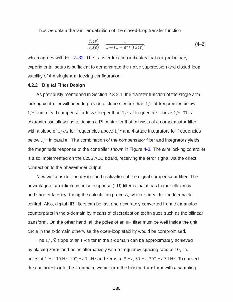
Thus we obtain the familiar definition of the closed-loop transfer function
φr(s)
φo(s)=
1
1 + (1− e−sτ)G(s), (4–2)
which agrees with Eq. 2–32. The transfer function indicates that our preliminary
experimental setup is sufficient to demonstrate the noise suppression and closed-loop
stability of the single arm locking configuration.
4.2.2 Digital Filter Design
As previously mentioned in Section 2.3.2.1, the transfer function of the single arm
locking controller will need to provide a slope steeper than 1/s at frequencies below
1/τ and a lead compensator less steeper than 1/s at frequencies above 1/τ . This
characteristic allows us to design a PI controller that consists of a compensator filter
with a slope of 1/√s for frequencies above 1/τ and 4-stage integrators for frequencies
below 1/τ in parallel. The combination of the compensator filter and integrators yields
the magnitude response of the controller shown in Figure 4-3. The arm locking controller
is also implemented on the 6256 ADC board, receiving the error signal via the direct
connection to the phasemeter output.
Now we consider the design and realization of the digital compensator filter. The
advantage of an infinite impulse response (IIR) filter is that it has higher efficiency
and shorter latency during the calculation process, which is ideal for the feedback
control. Also, digital IIR filters can be fast and accurately converted from their analog
counterparts in the s-domain by means of discretization techniques such as the bilinear
transform. On the other hand, all the poles of an IIR filter must be well inside the unit
circle in the z-domain otherwise the open-loop stability would be compromised.
The 1/√s slope of an IIR filter in the s-domain can be approximately achieved
by placing zeros and poles alternatively with a frequency spacing ratio of 10, i.e.,
poles at 1 Hz, 10 Hz, 100 Hz 1 kHz and zeros at 3 Hz, 30 Hz, 300 Hz 3 kHz. To convert
the coefficients into the z-domain, we perform the bilinear transform with a sampling
130

10−4
10−2
100
102
104
−60
−40
−20
0
20
40
60
Frequency (Hz)
Mag
nitu
de (
dB)
compensator filter4−stage integratorsoverall controller
Figure 4-3. The magnitude responses of the PI controller: The 4-stage integrators (red)dominate the frequencies below 1/τ ≈ 1 Hz to provide more suppressionand the compensator filter with a slope of 1/
√s (blue) dominates the
frequency band from 1 Hz to 10 kHz to reduce phase loss. For frequenciesbeyond the bandwidth (> 10 kHz) the compensator filter flattens out tomaintain the closed-loop stability.
frequency of 448 kHz, which is inherited from the data rate of the phasemeter output.
The IIR filter is implemented as a two-stage second-order-section (SOS) direct II form
filter. Since the filter is implemented on the FPGA which yields the fixed-point arithmetic,
the coefficients of the filter in the z-domain as well as the input and output values need
to be further quantized into fixed-point numbers, where the issues related to the limited
precision and the dynamic range arise. In practice, these issues are normally resolvable
and a balance between them can be obtained through empirical attempts. In this design,
the phasemeter sends 32-bit frequency data to the filter and during the entire data
transfer it is kept to be a 32-bit fixed-point value down to the NCO.
The magnitude response of the implemented IIR filter shown in Figure 4-4 is
measured by dividing the linear spectral densities of the input noise and the output
noise. It is worth noting that unlike the EPD unit, the output of the controller filter will not
be stored in the memory and then read out by the DAC board. In contrast, the output
signal will bypass the 4205 motherboard and directly received by the DAC board via VIM
131

100
102
104
−60
−50
−40
−30
−20
−10
0
10
20
Frequency (Hz)
Mag
nitu
de (
dB)
measuredtheoretical
Figure 4-4. The magnitude response of the 1/√s filter, where the measured transfer
function is very consistent with the theoretical design for frequencies below∼ 200 Hz. The high frequency noise (> 1 kHz) observed in the measurementis beyond the arm locking bandwidth.
10−2
100
102
104
10−4
10−2
100
102
104
Frequency (Hz)
Rel
ativ
e fr
eque
ncy
nois
e (H
z/rt
Hz)
Input frequency noise of laser beatResidual frequency noise of laser−NCO beat
10−2
100
102
104
10−4
10−3
10−2
10−1
100
101
Frequency (Hz)
Noi
se s
uppr
essi
on
measuredtheoretical
Figure 4-5. (Left) The measurement result of noise suppression performance at highfrequencies shows that compared with the initial frequency noise spectrumof the beat signal between two cavity stabilized lasers(blue), the residualfrequency noise spectrum of the laser-NCO beat (red) is suppressed by thecompensator filter. (Right) The closed-loop transfer function is given by theratio between the initial frequency noise spectrum and the residualfrequency noise spectrum.
transfer. This feature is enabled when the motherboard is set to the VIM-to-VIM data
transfer mode in order to minimize the data processing delay.
4.2.3 Measurement Results
After the arm locking starts and enters the steady state, we measure the phase
fluctuations of the initial beat signal φo(s) and the residual signal φr(s) using two
132

0 10 20 30 40 50 60−400
−300
−200
−100
0
100
200
300
Time (s)
Pha
se (
cycl
es)
Initial phase of the laser beatResidual phase of the laser−NCO beat
7 8 9 10 11 12 13 14 15−10
−8
−6
−4
−2
0
2
4
6
Time (s)
Pha
se (
cycl
es)
Figure 4-6. (Left) A 1 min time series of phase fluctuations of the initial beat signal(blue) and the residual laser-NCO beat (red) with a fast sampling frequencyof 61 kHz. (Right) A close-up of the residual laser-NCO beat. The time serieshave a distinct oscillation at about 1 Hz, as well as higher harmonics on thetop of it.
phasemeters individually. Here we have taken two kinds of phase measurements with
two different phasemeter data rates. The phasemeter first sends data at the high rate of
61.0 kHz for 60 s in order to investigate the noise suppression and the system bandwidth
at high frequencies. The linear spectral densities of the frequency noises are plotted in
Figure 4-5 (left), which shows a moderate noise suppression due to the compensator
filter for frequencies above 1 Hz. The ratio between them yields the magnitude of the
closed-loop transfer function, which displays multiple peaks at frequencies very close to
1 Hz, 2 Hz, 3 Hz, etc. The deviation from the theoretical transfer function mainly lies at
frequencies above 500 Hz, where a servo bump shows up at approximately 1 kHz. The
servo dump is ascribed to the excessive phase shift due to the propagation delay in data
transfer. Figure 4-6 plots the time series of the phase fluctuations within this time span.
Note that in this plot the linear drift due to a constant frequency value is already removed
from the phase data. Figure 4-6 (right) is the close-up of the residual phase fluctuations,
which distinctly exhibits an oscillation with a frequency very close to 1 Hz, as well as
other higher harmonics applied on it.
In the second set of phase measurements, the phasemeter runs at the low data rate
of 14.9 Hz for 15 hours to investigate the noise suppression performance in the LISA
133

10−4
10−2
100
10−6
10−4
10−2
100
102
104
Frequency (Hz)
Rel
ativ
e fr
eque
ncy
nois
e (H
z/rt
Hz)
Input frequency noise of laser beatResidual frequency noise of laser−NCO beat32−bit digitization noise floor
10−4
10−2
100
10−6
10−4
10−2
100
102
Frequency (Hz)
Noi
se s
uppr
essi
on
measuredidealized
Figure 4-7. (Left) The measurement result of noise suppression performance at lowfrequencies shows that compared with the initial frequency noise spectrumof the beat signal between two cavity stabilized lasers(blue), the residualfrequency noise spectrum of the laser-NCO beat (red) is suppressed by the4-stage integrators by 5 to 6 orders of magnitude from 0.1 mHz to 10 mHz.(Right) The closed-loop transfer function is given by the ratio between theinitial frequency noise spectrum and the residual frequency noise spectrum.The measurement has shown that the control system of this single armlocking loop is consistent with the theoretical design.
0 0.5 1 1.5 2 2.5 3 3.5 4 4.5
x 104
−2
−1.5
−1
−0.5
0
0.5
1
1.5
2x 10
6
Time (s)
Pha
se fl
uctu
atio
ns (
cycl
e)
Residual phase of the laser−NCO beatInitial phase of the laser beat
0 0.5 1 1.5 2 2.5 3 3.5 4 4.5
x 104
−6
−4
−2
0
2
4
6
Time (s)
Pha
se fl
uctu
atio
ns (
cycl
e)
Figure 4-8. (Left) A 12.5 h time series of phase fluctuations of the initial beat signal(blue) and the residual laser-NCO beat (red) with a slow sampling frequencyof 14.9 Hz. In this time span the initial phase fluctuates by more than3.5× 106 cycles. (Right) A close-up of the residual laser-NCO beat. Theresidual phase fluctuates by about 10 cycles and the general profileresembles the initial phase fluctuations, indicating that the noise suppressionat low frequencies is limited.
134

Figure 4-9. Single arm locking with NCO tracking - Laplace domain with noise sources.This single arm locking loop has four primary error input points. Note thatthe noise sources introduced outside the arm locking controller are treatedas the phase noise and otherwise the frequency noise, in accordance withthe convention used in Figure 4-2.
band. The linear spectral densities of the initial frequency noise and residual frequency
noise, and the time series of the phase fluctuations are shown in Figure 4-7 (left) and
Figure 4-8, respectively. The ratio between the two spectra yields the magnitude of
the closed-loop transfer function, which indicates 5 to 6 orders of magnitude noise
suppression from 0.1 mHz to 10 mHz as shown in Figure 4-7 (Right).
The closed-loop transfer function shown in Figure 4-7 (Right) yields a s3 slope from
10 mHz to 0.1 Hz due to the 4-stage integrators in the controller. The measurement
result agrees well with the theoretical design, which indicates that the noise suppression
performance is gain limited in this frequency region. However, for frequencies below
10 mHz the result shows an obvious deviation as the closed-loop transfer function
flattens out rather than continue decreasing with a s3 slope. This behavior indicates
that in this frequency region the suppression performance is limited by a different noise
source. As shown in Figure 4-7 (Left), the deviation in the closed-loop transfer function
is caused by the 1/s slope in the residual frequency noise spectrum.
135

4.2.4 Noise Analysis
To analyze the noise limits and determine the dominating noise floor in the setup,
we consider possible noise sources in Figure 4-2 and then draw Figure 4-9. These noise
sources include the 48-bit digitization noise δϕ48−dig and the ADC jitter ϕADC introduced
at the EPD unit as well as the arm locking phasemeter, which are represented as phase
noises in the figure; any Doppler frequency mismatch introduced at the arm locking
phasemeter, which is also represented as a phase noise δωD · t; the 32-bit digitization
noise δf32−dig at the feedback filter, which is represented as a frequency noise; as well as
frequency noise δfNCO introduced by the NCO.
Among these noise sources, it is obvious that any NCO noise δfNCO will be
suppressed by the open-loop gain. Since the Doppler shift frequency is designed
to be perfectly accounted for by the phasemeter preset frequency, the phase noise
representing the Doppler frequency error also vanishes. The 48-bit digitization noise and
the ADC jitter added at the EPD unit will be tracked by the residual signal; however, they
are at a fairly low level compared with the 1/s slope. Actually, the calculation indicates
that the 1/s slope is an effect of the 32-bit digitization noise added in the feedback filter,
where the 32-bit frequency fluctuation is sampled at 488 kHz. Thus we determine the
digitization noise
NDig =fclock · 2−N√6 · fs
= 8.50× 10⁻⁶ Hz Hz−1/2. (4–3)
In terms of frequency noise the digitization noise is white through the entire band.
As this frequency noise becomes an additional term in the error signal transfered from
the phasemeter to the filter, it has an equivalent effect as the Doppler frequency error
entering and being accumulated by the closed-loop. Therefore in the presence of a
DC-coupled controller, the digitization noise multiplied by 1/s will appear in the spectrum
of the residual frequency noise and the level of the noise floor scales with 1/τ :
δνDig(f ) =Ndig
τs=1.35× 10⁻⁶
fHz Hz−1/2. (4–4)
136

10−3
10−2
10−1
100
101
10−4
10−2
100
102
104
Frequency (Hz)
Rel
ativ
e fr
eque
ncy
nois
e (H
z/rt
Hz)
free−running VCO frequency noiseresidual VCO−NCO beat frequency noise30−bit digitization noise floor 32−bit digitization noise floor
Figure 4-10. The dashed green noise floor is given by the 30-bit digitization noisecoupled into the single arm locking loop. Compared with the 32-bitdigitization noise floor (dashed black), the dashed green floor is higher by afactor of 4 since the precision given by the lowest two bits is lost in thefrequency information. The measurement has shown that the noisesuppression is limited by the new noise floor when the 30-bit arm lockingcontroller is used.
As shown in Figure 4-7, this noise floor accurately matches up the 1/s slope in
the residual frequency spectrum. This noise floor can further be verified by changing
the delay time or changing the fixed-point precision of the frequency fluctuations. To
demonstrate the influence of the precision to the level of the noise floor, we truncate
the 32-bit frequency fluctuation in the filter to 30-bit by hard coding the values of the
lowest two bits to zero. We take the measurement using a free-running VCO as the
input noise and the result of the 30-bit filter is shown in Figure 4-10. The result explicitly
demonstrates that the measured 30-bit digitization noise floor agrees with the theoretical
prediction that the new noise floor increases by a factor of 4 due to the 2-bit precision
loss in the filter.
Since the digitization noise in the feedback filter is equivalent to a Doppler
frequency error at the phasemeter, the direct consequence of this 1/s noise floor in
the time domain is a linear drift in the output frequency. Here a higher digitization noise
137

0 500 1000 1500 2000 2500 3000 3500−20
0
20
40
60
80
100
120
Time (s)
Fre
quen
cy d
rift (
Hz)
filter with 32−bit frequency fluctuationfilter with 30−bit frequency fluctuation
Figure 4-11. Comparison of frequency drift rate between a 30-bit filter (28.6 mHz/s) anda 32-bit filter (7.5 mHz/s). The frequency drift rate of a 30-bit filter is largerby a factor of about 4, scaling with the rms amplitude of the digitizationnoise.
floor corresponds to a faster frequency drift, as illustrated in Figure 4-11. The frequency
data in this figure has been low-pass filtered by averaging out the high frequency noise
(e.g., using a boxcar filter) such that the linear drift can be explicitly revealed. The
linear regression approach shows that for the 32-bit filter the frequency drift rate is
approximately 7.5 mHz/s and for the 30-bit filter it is approximately 28.6 mHz/s, which
is again roughly four times the drift rate of the 32-bit case. Given that in realistic LISA
the light travel time on one arm is approximately 33 times larger than the 1 s delay time
in our experiment, the 32-bit digitization noise should not have significant effects on the
noise suppression performance or frequency pulling if single arm locking is used.
4.3 Single Arm Locking Integrated with a Tunable Reference
In this section we move forward to the authentic electro-optical models where single
arm locking is used to stabilize the laser frequency. The incorporation of arm locking and
pre-stabilization subsystem requires an additional actuator to tune the pre-stabilization
reference. The specific approaches have been already introduced in Section 2.3.4 and
so far, all proposed methods to integrate single arm locking with Pound-Drever-Hall
technique have been experimentally demonstrated on UFLIS. Instead of the preliminary
138

verification of the noise suppression performance and closed-loop stability in the
previous electronic model, we will focus on the characterization of the tunable references
and additional noise sources introduced by them in these more realistic single arm
locking demonstrations.
4.3.1 Heterodyne Phase-locked Loop
The actuation method of heterodyne phase-locking requires an auxiliary laser
to faithfully reproduce the laser frequency noise of the cavity stabilized laser. For
this reason it is not a concise option for realistic LISA, yet it is a simple approach to
demonstrate in benchtop experiments.
4.3.1.1 Experimental setup
As described in Figure 2-27, the concept of PLL-based single arm locking is to
stabilize an auxiliary laser which is phase-locked to the cavity stabilized laser such
that the local oscillator of the PLL can be tuned by the arm locking controller. The
bench-top experimental setup of the PLL-based single arm locking resembles the
setup in Figure 2-27 except that we use another cavity stabilized laser RL to generate
a beat signal against the phase-locked laser. Figure 4-12 illustrates the experimental
setup in which the reference laser RL and the master laser L1 are cavity stabilized via
Pound-Drever-Hall technique. The slave laser L2 is phase-locked to L1 with a frequency
offset, which is driven by the NCO in the arm locking controller. Therefore, the stability
of the cavity stabilized laser L1 is transfered into L2 through phase-locking and the
frequency noise in the RL− L2 beat signal is approximately equal to the frequency noise
in the beat signal RL − L1. Also, due to the heterodyne PLL the stability of the beat
signal RL − L2 is tunable, which means it can be further stabilized by a more stable
reference: the arm length (i.e., the fixed delay time in our experiment). Compared with
the preliminary test with NCO tracking the input noise, the frequency of the laser beat
signal RL− L2 is directly suppressed by the arm locking open-loop gain.
139

Figure 4-12. The experimental setup of single arm locking experiment using anadditional heterodyne phase-locked laser. In this setup the reference laserRL and the master laser L1 are cavity stabilized via Pound-Drever-Halltechnique. The slave laser L2 is phase-locked to L1 with a frequency offset,which is driven by the NCO in the arm locking controller. Therefore, withinthe PLL bandwidth L2 faithfully reproduces the laser frequency noise of L1,both referenced to the “optical clock” RL. Note that the PLL bandwidth isabout 20 kHz, which is well larger than the arm locking bandwidth(∼ 1 kHz); therefore it will not limit our arm locking performance and a directfeedback of the arm locking control signal to the laser is not necessary. Thearm locking controller is used to adjust the NCO that drives the PLL and thefrequency noise of L2 can be further suppressed by the arm lockingcontroller gain.
In our experiment the nominal frequency of the RL− L1 beat signal is approximately
13 MHz. If we set the nominal frequency of the NCO signal to be 8 MHz and phase-lock
L2 to L1, there will be two possibilities for the nominal frequency of the the RL − L2 beat
signal: 5 MHz and 21 MHz, depending on which value is larger between the nominal
frequencies of L1 and L2. Only one of the two beat frequency values is working for
the setup as the other configuration would yield a wrong sign. In our setup the right
configuration is a 5 MHz RL − L2 beat signal. The EPD unit is configured in the same
way as for the NCO tracking setup, providing a 1 s delay time and −2 MHz Doppler shift.
140

Figure 4-13. The closed-loop dynamics of single arm locking tuned by a heterodyne PLLin the Laplace domain. The control system is based on two loops: PLL andsingle arm locking. The stability of the arm locking reference is transferredinto the error signal of the PLL via the driving NCO.
4.3.1.2 Closed-loop dynamics
Figure 4-13 illustrates the experimental setup represented in the Laplace domain.
In this diagram we use Φi to represent the phase of the laser Li (The laser phase of a
free-running L2 is given by Φ02 and the in-loop phase of the phase-locked (and then arm
locked) L2 is given by Φ2.) and ϕ to represent the phase of the PLL feedback, the phase
of the NCO signal, etc. Note that in this diagram the configuration of the plus and minus
signs assumes the nominal frequencies of the three lasers yield ΩRL > ΩL2 > ΩL1 .
Not all permutations of the three frequencies are allowed for the system stability and
different permutations will result in different configuration of the plus and minus signs.
If we consider the phase-locked loop, the relations are given by
Φ2 = Φ02 − ϕPLL
ϕPLL = (Φ2 −Φ1 − ϕNCO)GPLL. (4–5)
Hence we solve the in-loop phase of L2 given by
Φ2 =1
1 + GPLLΦ02 +
GPLL
1 + GPLL(Φ1 + ϕNCO). (4–6)
141

The first term represents the initial noise suppressed by the open-loop gain and
the second term represents the reference noise that this PLL tracks, i.e., the slave laser
L2 tracks the master laser L1. A phase modulation ϕNCO from the NCO signal is also
coupled into the PLL reference. The tunability of ϕNCO allows the phase of L2 can be
further stabilized.
In the arm locking loop, the NCO noise is given by
ϕNCO = (Φ0 −Φ2)(1− e−sτ)GAL. (4–7)
Substitute Eq. 4–7 into Eq. 4–6 and we have
Φ2 =1
1 + GPLLΦ02 +
GPLL
1 + GPLL(Φ1 + (Φ0 −Φ2)(1− e−sτ)GAL)
=1
1 + GPLLΦ02 +
GPLL
1 + GPLLΦ1 +
(Φ0 −Φ2)(1− e−sτ)1 + GPLL
GPLLGAL. (4–8)
We combine the terms involving Φ2 to the left and add terms Φ0 − 11+GPLL
Φ0 −GPLL1+GPLL
Φ0 (= 0) to the right:
[1 +
GPLL
1 + GPLL(1− e−sτ)GAL
]Φ2 = (4–9)
1
1 + GPLLΦ02 +
GPLL
1 + GPLLΦ1 +
Φ0(1− e−sτ)1 + GPLL
GPLLGAL +Φ0 −1
1 + GPLLΦ0 −
GPLL
1 + GPLLΦ0.
(4–10)
The purpose of these additional terms is such that the above equation can be
simplified into
[1 +
GPLL
1 + GPLL(1− e−sτ)GAL
](Φ2 −Φ0) =
1
1 + GPLL(Φ02 −Φ0) +
GPLL
1 + GPLL(Φ1 −Φ0),
(4–11)
where Φi − Φ0, i = 1, 2 is the phase of the beat signal, i.e., the phase of L1,2 relative to
the reference laser RL. From this equation we obtain the equivalent open-loop transfer
function
TFOL =GPLL
1 + GPLL(1− e−sτ)GAL. (4–12)
142

The first term on the right indicates that the phase noise of a free-running L2 relative
to the reference laser is double suppressed by the open-loop gain of phase locking as
well as that of arm locking. The second term on the right, which was tracked in phase
locking, is now suppressed by the open-loop gain of arm locking. In the high gain limit
(GPLL ≫ 1) of the PLL, 11+GPLL
≈ 0 and GPLL1+GPLL
≈ 1, then Eq. 4–12 approximates to the
open-loop transfer function in Eq. 4–2 and Eq. 4–11 is further reduced into
[1 + (1− e−sτ)GAL
](Φ2 −Φ0) = Φ1 −Φ0. (4–13)
Finally, the closed-loop transfer function is given by
TFCL =1
1 + (1− e−sτ)GAL=Φ2 −Φ0Φ1 −Φ0
. (4–14)
This relation indicates the phase noise of RL − L2 beat signal is suppressed from
the noise level of RL− L1 by the arm locking open-loop gain and the closed-loop transfer
function of the entire system can be approximately given by the ratio between them. In
other words, the PLL-based single arm locking setup is mathematically equivalent to the
preliminary experiment of NCO tracking in the presence of an ideal PLL.
4.3.1.3 Results and analysis
We measure the frequency noises of the RL − L1 beat signal and the RL − L2beat signal as the input noise and the output noise, respectively. Their noise spectra
in the low frequency region are shown in Figure 4-14. As seen in the figure, the noise
spectrum of the RL − L2 is almost identical to the residual frequency noise shown in
Figure 4-7 (left), except for some difference in the overall loop gain. The measured
closed-loop transfer function, which is given by the ratio between the two spectra,
indicates that the RL−L2 beat signal has been stabilized with 5 to 6 orders of magnitude.
In the low frequency region the noise suppression is again limited by the same 32-bit
digitization noise floor described in Section 4.2.4.
143

10−4
10−3
10−2
10−1
100
101
10−4
10−2
100
102
104
106
Frequency (Hz)
Rel
ativ
e fr
eque
ncy
nois
e (H
z/rt
Hz)
Frequency noise of RL−L1 beat signalFrequency noise of RL−L2 beat signal32−bit digitization noise floor
10−4
10−3
10−2
10−1
100
101
10−6
10−4
10−2
100
Linear Spectral Density
Frequency (Hz)
Noi
se s
uppr
essi
on
measuredidealized
Figure 4-14. (Left) The noise spectra of the initial RL− L1 beat signal (blue) and thestabilized RL− L2 beat signal (red). The noise suppression performance isalmost identical to the result given by Figure 4-7. (Right) The closed-looptransfer function given by the ratio between the two LSDs is also the sameas the previous experiment. The deviation from the theoretical design againcomes from the 32-bit digitization noise floor.
In addition to the 32-bit digitization noise and ADC noise already mentioned in
Section 4.2.4, the phase-locked loop in this setup also introduces spurious phase
variations δϕPLL into the error signal. Also, the uncertainty in the lightpath length from
the laser to the photodiode results in the uncertainty in the laser phase; therefore, the
L1 − L2 beat signal and the RL − L2 beat signal will have uncorrelated lightpath noises
δϕLP12 and δϕLP02 attributed to the difference in the lightpath of each laser. We need to
investigate the influence of these noise sources to the measurement result as well. The
noise model in the Laplace domain is drawn as Figure 4-15.
It is straightforward to show that the phase of L2 also tracks the PLL noise δϕPLL in
the PLL:
Φ2 =1
1 + GPLLΦ02 +
GPLL
1 + GPLL(Φ1 + ϕNCO + δϕPLL), (4–15)
which indicates that the PLL noise is simply coupled into the phase noise of L1.
Although it increases the noise level of L2 from the point of view of the phase-locked
loop, the phase noise of the RL − L1 beat signal, including this PLL noise, is well
suppressed by the arm locking open-loop gain. This demonstrates that any noise
144

Figure 4-15. Single arm locking with heterodyne PLL - Laplace domain with noisesources. In addition to the noise sources analyzed in Figure 4-9, theheterodyne PLL actuator also introduces the PLL noise δϕPLL, as well asthe lightpath noise δϕLP12 and δϕLP02.
introduced by the PLL will be adequately suppressed and unlikely cause a limitation in
the arm locking performance.
The same situation is for the lightpath noise δϕLP12 and δϕLP02, which is coupled into
the L1 − L2 beat signal and RL − L2 beat signal individually. The existence of the light
noise δϕLP12 and δϕLP02 is nothing more than an additional term added in ϕPLL and ϕNCO,
i.e.,
ϕPLL = (Φ2 −Φ1 + δϕLP12 − ϕNCO)GPLL
ϕNCO = (Φ0 −Φ2 + δϕLP02)(1− e−sτ)GAL. (4–16)
In other words, they can be considered as being coupled into the phase noise Φ1
and Φ0, respectively. δϕLP12, as a small portion of Φ1, will again be suppressed by the
arm locking open-loop gain. However, δϕLP02 coupled in the reference laser will show up
in all the beat signals and then increases the stabilized noise of RL − L2 beat signal by
an insignificant amount.
145

4.3.2 Piezoelectric Transducer (PZT) Actuated Cavity
The PZT actuated cavity is a straightforward concept to continuously tune the
frequency of a cavity stabilized laser by actively modulating the cavity length. The
advantage of a PZT cavity is that the modification to the optical cavity does not
significantly complicate the implementation while still could achieve considerable tuning
range. Although the PZT actuator will inevitably compromise the reference stability of
pre-stabilization by probably one order of magnitude, the incorporation with arm locking
is capable of suppressing the noise significantly well below the requirement.
4.3.2.1 Characterization of the PZT cavity
In a PZT actuated cavity, a PZT actuator is used to change the distance between
the two mirrors forming the reference cavity. In our experiment the PZT actuator is
placed between the fused silica mirror and the Zerodur spacer of the cavity using
hydroxide bonding. This additional PZT actuator compromises the stability of the cavity
length: Measurements have shown that the frequency noise of the beat signal between
two lasers, which are locked to a standard Zerodur cavity and a PZT cavity individually,
is approximately on the level of ∼ kHz Hz−1/2 at 1 mHz, with an applied voltage from 0 V
to 100 V. With the voltage increased from 100 V to 200 V, the frequency noise will also
increase slightly. The typical frequency drift rate of the beat signal has been observed to
be within the range of 50 ∼ 350 Hz/s. 1
The feedback signal arriving at the PZT actuator has to be a DC signal. Since
the NCO in the controller is AC-coupled, we program another NCO generating a
free-running signal with the same nominal frequency and then use an analog mixer to
generate a DC output by means of demodulation. The DC-coupled error signal is used
to drive the PZT actuated cavity. When the arm locking loop is closed, the frequency of
1 The hydroxide bonding of the PZT cavity as well as the characterizationmeasurements described in this paragraph are done by Alix Preston.
146

the error signal is close to DC. In this region a small change in phase can be considered
linearly proportional to a small change in the voltage applied on the PZT actuator, i.e.,
dV = Kdϕ, where K is the conversion coefficient determined by the analog mixer. Using
the full range of the DAC, the conversion coefficient was found to be approximately
3.2 mV/degree.
Consequently, the PZT actuator converts the change in voltage into a change in the
cavity length. This conversion is also almost linear at frequencies below 20 kHz. The
cavity length change then results in the change of the resonant frequency. As we know,
the relation between the resonant frequency ΩL of a reference cavity and its optical path
length L is given by
ΩL =2πnc
L. (4–17)
By taking the first-order derivative on both sides, we obtain the relation between the
change in the resonant frequency and the change in the optical length:
dΩL = −2πncL2dL. (4–18)
The linear conversion from the applied voltage to the change in the resonant
frequency can be described using a tuning coefficient, which is measured to be ∼
1.5 MHz/V. As previously mentioned in Section 2.3.4, the tuning range for the tunable
reference is required to be at least tens of MHz. If the desired tuning capability is
designed to be 100 MHz, the applied voltage is then required to have a range of 0 ∼
70 V, which generally requires a low-noise DC amplifier to amplify the feedback signal.
If we take the conversions starting from the NCO output to the resonant frequency
change as a whole, it is essentially a conversion from the phase change to the
frequency change. This conversion resembles the frequency actuator in laser controllers,
which actuate the phase change from the controller signal into the laser frequency
change. Since a frequency actuator is equivalent to a phase actuator with a 1/s factor,
147

Figure 4-16. The experimental setup of single arm locking experiment using a PZTactuated cavity. In this setup the reference laser RL is locked to a standardcavity and the main laser L1 is locked to the PZT cavity. Their beat signal isfirst demodulated by a function generator signal to the desired frequencyrange and then sent into the control system of single arm locking. As thePZT actuator needs the feedback signal at DC, a second free-running NCOis used to demodulate the NCO signal that is adjusted by the arm lockingcontroller. Note that the controller filter is multiplied with s in the transferfunction to compensate the phase-to-frequency conversion in the PZTactuator.
the PZT actuated cavity contains an intrinsic 1/s integrator that must be taken into
account in closed-loop dynamics.
4.3.2.2 Experimental setup
The experimental verification of PZT-actuated single arm locking is illustrated
by Figure 4-16. In this setup the main laser L1 is stabilized to a PZT actuated cavity
via Pound-Drever-Hall technique. Another pre-stabilized reference laser RL, which is
locked to a standard Zerodur cavity with a fixed length, is used to generate a 81 MHz
heterodyne beat signal with L1 at the photodiode. This beat signal is demodulated by
a 72 MHz function generator signal to 9 MHz, which is sent into the arm locking sensor
with 1 s delay and then appropriately filtered by the controller. As mentioned in the
148

Figure 4-17. The closed-loop dynamics of single arm locking tuned by a PZT actuatedcavity in the Laplace domain. The closed-loop dynamics of thisexperimental setup is simple as the arm locking feedback signal is directlysent back to the laser via the PZT actuator. Compared with Figure 4-2, themain difference is the additional gain stages and the intrinsic integrator inthe PZT actuation.
previous section, the controller is configured to have two parallel NCOs running at the
same 5 MHz nominal frequency. The difference between them is that one NCO receives
the filtered frequency fluctuations from the arm locking error signal, while the other
NCO is free-running to demodulate the first NCO signal. The output of the analog mixer
carries the information of the phase fluctuations, which is already converted into a DC
voltage. After appropriately amplified to ∼ 70 V, the voltage is applied onto the PZT
actuator to modulate the optical length of the cavity. The modulation on the cavity length
is then used to correct the resonant frequency that L1 is locked to.
Due to the intrinsic 1/s integrator in the PZT actuator, the controller filter needs to
be modified by multiplying an s slope to maintain the closed-loop stability. The controller
filter in this setup is designed to have a√s slope to provide 45 phase advance, which
can be realized by switching the frequencies of zeros and poles in the 1/√s filter.
The experiment model in the Laplace domain is shown in Figure 4-17. In this model
the controller output is followed by a series of gain stages, where K0 represents the
149

amplifier gain, K1 represents the conversion from the phase to the voltage at the analog
mixer, K2 represents the conversion from the voltage to the resonant frequency at the
PZT actuator. To properly close the loop, another 1/s stage is required to convert the
frequency back to the phase. Therefore, the relations to describe this model are given by
Φ1 = Φ01 − ϕPZT
ϕPZT = (Φ1 −Φ0)(1− e−sτ)K0K1K2G
s. (4–19)
If we define the open-loop transfer function
TFOL = (1− e−sτ)K0K1K2G
s, (4–20)
The stabilized phase noise of L1 is then given by
Φ1 =1
1 + TFOLΦ01 +
TFOL
1 + TFOLΦ0. (4–21)
Since we are more concerned with the phase noise of the RL − L1 beat signal,
Eq.4–21 is equivalent to
TFCL =Φ1 −Φ0Φ01 −Φ0
=1
1 + TFOL. (4–22)
4.3.2.3 Results and analysis
The measurement results of the frequency noise are shown in Figure 4-18.
According to the noise spectra, although the frequency noise of the beat signal
stabilized by a free-running PZT cavity does not meet the stringent 30 Hz Hz−1/2
pre-stabilization requirement, single arm locking is capable of appropriately tuning
the PZT cavity such that the noise spectrum is significantly reduced by 6 or 7 orders
of magnitude. Note that even in the gain limited region, the initial frequency noise
and the stabilized frequency noise are not correlated since they were not measured
simultaneously. Nevertheless, we modeled the open-loop transfer function of the setup
given by Eq. 4–20 and the idealized stabilized noise spectrum, represented by the green
150
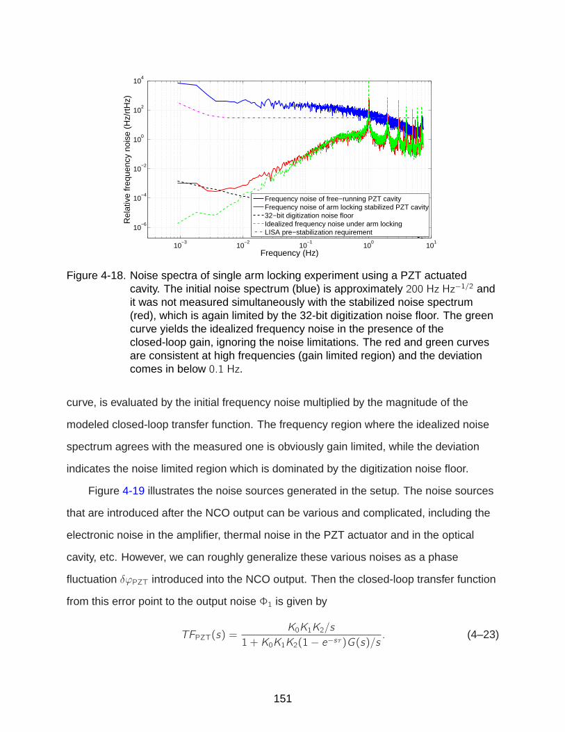
10−3
10−2
10−1
100
101
10−6
10−4
10−2
100
102
104
Frequency (Hz)
Rel
ativ
e fr
eque
ncy
nois
e (H
z/rt
Hz)
Frequency noise of free−running PZT cavityFrequency noise of arm locking stabilized PZT cavity32−bit digitization noise floorIdealized frequency noise under arm lockingLISA pre−stabilization requirement
Figure 4-18. Noise spectra of single arm locking experiment using a PZT actuatedcavity. The initial noise spectrum (blue) is approximately 200 Hz Hz−1/2 andit was not measured simultaneously with the stabilized noise spectrum(red), which is again limited by the 32-bit digitization noise floor. The greencurve yields the idealized frequency noise in the presence of theclosed-loop gain, ignoring the noise limitations. The red and green curvesare consistent at high frequencies (gain limited region) and the deviationcomes in below 0.1 Hz.
curve, is evaluated by the initial frequency noise multiplied by the magnitude of the
modeled closed-loop transfer function. The frequency region where the idealized noise
spectrum agrees with the measured one is obviously gain limited, while the deviation
indicates the noise limited region which is dominated by the digitization noise floor.
Figure 4-19 illustrates the noise sources generated in the setup. The noise sources
that are introduced after the NCO output can be various and complicated, including the
electronic noise in the amplifier, thermal noise in the PZT actuator and in the optical
cavity, etc. However, we can roughly generalize these various noises as a phase
fluctuation δϕPZT introduced into the NCO output. Then the closed-loop transfer function
from this error point to the output noise Φ1 is given by
TFPZT(s) =K0K1K2/s
1 + K0K1K2(1− e−sτ)G(s)/s. (4–23)
151

Figure 4-19. Single arm locking with a PZT actuated cavity - Laplace domain with noisesources. Compared with Figure 4-9, the PZT actuation introducesadditional noise sources such as the electronic noise, thermal noise, etc.These noise sources can be generalized as the phase noise δϕPZTintroduced after the NCO output, and are consequently suppressed by theclosed-loop gain.
At low frequencies, it is easy to show that this transfer function approximates to
1(1−e−sτ )G(s) such that any phase noise introduced after the NCO output is still well
suppressed by the integrator gain.
4.3.3 Electro-optic Modulator (EOM) Sideband Locking
In addition to the two tunable references described above, the experimental
verification of single arm locking with EOM sideband locking has also been demonstrated
on UFLIS. The experiment was performed by Jeffery Livas et al.at Goddard Space Flight
Center (GSFC) [94], incorporating the arm locking components on UFLIS and the
pre-stabilization system including the broadband EOM provided by GSFC. In the
setup a sideband generated at the EOM is locked to the fixed length cavity using the
standard PDH technique. Tunability is achieved by changing the frequency of the phase
modulation signal applied on the EOM and the local oscillator, which both need to be
152

broadband. In the experiment, the tunable range of the entire control system is limited
by the tunability of the local oscillator to a few tens of MHz.
This experiment has demonstrated additional noise suppression can be achieved
by the incorporation of single arm locking and sideband locking as the tunable
pre-stabilization reference, which only requires minimal modifications to the PDH
cavity stabilization and does not explicitly degrade the noise suppression performance of
it.
153

CHAPTER 5EXPERIMENTAL VERIFICATION OF DUAL/MODIFIED DUAL ARM LOCKING
5.1 Common Arm Locking
In this chapter we discuss the experimental verification of advanced arm locking
configurations that utilize the interferometer outputs on both two LISA long arms,
including common arm locking, dual arm locking and modified dual arm locking [15].
Among these configurations, although common arm locking takes a linear combination
of the phasemeter measurements on both arms, it still resembles single arm locking in a
variety of ways such that it has never been considered promising. Nevertheless, we will
still first demonstrate the validity of common arm locking with relatively short time delays
on UFLIS. The reason is that as the simplest two-arm configuration, the common arm
locking experiment can be considered as a preliminary test for the follow-on arm locking
experiments with more elaborated linear combinations.
5.1.1 Common Arm Locking Sensor
Based on the discussion in Section 2.3.2.2, the common arm sensor is essentially
given by the sum of two long arm interferometry outputs on two different arms. In the
realistic architecture, the phase noise of the long arm interferometry on each arm is
fast sampled and then measured by the controller phasemeter individually. A mapping
vector, which is an adder for the case of common arm locking, will be implemented
right behind the phasemeters to generate an sensor/error signal. For our simulation on
UFLIS, the long arm interferometry is represented by electronic mixing of the prompt
and EPD-delayed phase. To generate differential light travel time between two LISA
arms, the EPD unit will need to exploit the bottom VIM on the Pentek board where the
delay buffer can be specified with a different array length.
As shown in Figure 5-1 (left), the common arm sensor of UFLIS is implemented
on two Pentek boards which function respectively as front end and back end. The front
end includes two EPD units that simulate the round-trip travel time on two different
154

10−4
10−3
10−2
10−1
100
101
10−2
10−1
100
101
Frequency (Hz)
Mag
nitu
de
Figure 5-1. (Left) The design of the common arm locking sensor on the FPGA. Thecommon arm sensor is implemented on two Pentek boards. DSP board 1functions as the round-trip delay lines on two arms and DSP board 2functions as the phase measurements and the mapping vector on the localspacecraft. The phasemeters send the frequency data with a fast rate of488 kHz. (Right) The measured common arm sensor transfer function. Theaveraged delay time is 5 s and the differential delay time is 0.1 s. Note thatthe first sensor null is at 1/∆τ = 10 Hz, which is higher than the Nyquistfrequency of this measurement. The measured transfer function only havelocal minima at n/τ .
arms individually. We use an voltage controlled oscillator as a noisy oscillator for initial
experiments. The VCO signal is electronically split into two arms and the signal on each
arm is split again to generate a prompt signal and a delayed and Doppler shifted signal
via the EPD unit. On the other Pentek board the back end starts with two phasemeters
that measures the phase difference on each arm individually. Identical to the single arm
locking case, the phasemeter design is optimized in a way that they send data with a
fast rate of 488 kHz to minimize the data transfer delay. The mapping vector calculates
the sum of the two phase measurements and then send the 32-bit error signal into the
following controller filter.1
For the purpose of demonstration, the delay provided by the EPD units are set to
be relatively short times such as 2 s or 5 s. The reason is simply that the design of the
1 The phasemeter measures the frequency fluctuations and send out the data witha precision of 48-bit. Then the 48-bit data is truncated in the VHDL code and only high32-bit has been kept before they are received by the mapping vector.
155

Figure 5-2. The experimental setup of common arm locking using an NCO to track theinput noise. The basic configuration resembles the setup in Figure 4-1. Thedelay times are 2.1 s and 1.9 s.
controller filter for single arm locking experiments can be directly adapted for common
arm locking with similar delay times, while a common arm locking demonstration with
realistic 33 s delay would only be compatible with a totally different set of zeros and
poles to be designed in the controller filter. Figure 5-1 (right) shows the measurement
of the magnitude response of a common arm locking sensor with delay times 5.1 s
and 4.9 s (τ = 5 s and ∆τ = 0.1 s). The magnitude response has nulls starting from
1/(∆τ) = 10 Hz, which is already beyond the LISA band; however, there are also local
minima at multiples of 1/τ = 0.2 Hz where each phase shift is still close to π/2 with
various degrees.
5.1.2 Preliminary Test with Numerical Control Oscillator (N CO) Tracking
The experimental setup to demonstrate the control system of common arm locking
is shown in Figure 5-2, which is identical to the setup described in Figure 4-1 except for
the replacement with the common arm sensor. In this experiment the delay times are
set to be 2.1 s and 1.9 s. By following similar procedures discussed in Section 4.2.1, the
residual phase noise ϕr(s) is given by
ϕr(s) = ϕo(s)−G(s)
1 + HC(s)G(s)Sk ·Φ1(s), (5–1)
156

10−4
10−3
10−2
10−1
100
101
10−6
10−4
10−2
100
102
104
Frequency (Hz)
Rel
ativ
e fr
eque
ncy
nois
e (H
z/rt
Hz)
Free−running VCOVCO−NCO beat signal32−bit digitization noise − 2 s
10−4
10−3
10−2
10−1
100
101
10−8
10−6
10−4
10−2
100
Frequency (Hz)
Noi
se s
uppr
essi
on
measuredidealized
Figure 5-3. (Left) The noise spectra of the free-running VCO signal (blue) and theVCO-NCO beat signal (red). The noise spectrum of the residual frequencynoise is limited by the 32-bit digitization noise floor, which is given by theintegrated quadrature sum of the 32-bit digitization noise from the twoindependent phasemeter. (Right) The closed-loop transfer function is givenby the ratio between the two noise spectra.
Then the closed-loop transfer function is given by
ϕr(s)
ϕo(s)=
1
1 + (2− e−sτ2 − e−sτ3)G(s). (5–2)
The measurement results of the original noise and residual noise, as well as the
closed-loop transfer function given by the ratio between them, are shown in Figure
5-3. Due to the local minima at n/τ in the sensor magnitude response, the residual
frequency spectrum still exhibits periodic peaks, although not noise enhancements, at
these frequencies and at 1/τ = 0.5 Hz the peak reaches the highest.
In the low frequency region, the noise suppression is again limited by the 32-bit
digitization noise floor. The experiment model in the Laplace domain is shown in
Figure 5-4, which depicts a generic arm locking configuration with NCO tracking. In
this diagram the block labeled with “mapping vector” represents an adder for common
arm locking. Note that the ADC noise and the digitization noise introduced on different
arms is uncorrelated to each other. Based on the discussion in Section 2.3.5.2, the
arm locking sensor will detect the common noise between two arms, which is given by
the quadrature sum of them. Since the digitization noises in two arms are uncorrelated
but have the same amplitude in our setup, the quadrature sum is given by√2Ndig. The
157

Figure 5-4. The closed-loop dynamics of common arm locking with NCO tracking in theLaplace domain. This diagram can represent the control system of anytwo-arm-based arm locking configuration, where the block labeled withmapping vector determines the specific arm locking type. Note that the samekind noise sources (digitization noise, ADC noise) between the two channelsare uncorrelated and their common noise is given by the quadrature sum ofthem.
magnitude response of the common arm locking loop to the common digitization noise
scales with 1/τ , therefore we have
δνDig(f ) =
√2Ndigτs
=9.53× 10⁻⁷
fHz Hz−1/2. (5–3)
Compared with the single arm locking experiments, the digitization noise floor has
been decreased by a factor of√2 due to the longer averaged delay time. For realistic
33 s light travel time, the digitization noise floor can be further decreased for single
or common arm locking and hence should not cause significant impact on the noise
suppression performance.
158

0 50 100 150 200−2
−1.5
−1
−0.5
0
0.5
1
1.5
2
Time (s)
Fre
quen
cy v
aria
tion
(Hz)
Figure 5-5. The lock acquisition process observed in the common arm lockingexperiment. The start-up transients caused by a non-zero initial error signalappear in the time series with a period of 2 s. The transients decay with atime constant less than 50 s; however, this observed time constant is basedon an averaged light travel time of 2 s. For a 33 s round-trip travel time, thetime constant would increase proportionally and become comparable to thesingle arm locking case.
Analogous to single arm locking, the periodic impulse peaks are also visible in
the time series and the most distinguishable oscillation yields a period of 2 s. Figure
5-5 illustrates the measurements in the first couple of minutes, where the start-up
transients with a period of 2 s appear in the lock acquisition process and decay with a
time constant less than 50 s. Note that the time scale used in our experiment is shorter
than the realistic LISA situation by a factor of about 16. Therefore, the expected time
constant for a realistic 33 s delay is on the level of more than 500 s, which is comparable
to the single arm locking model described in Figure 2-13.
5.2 Dual Arm Locking
5.2.1 Dual Arm Locking Sensor
As an enhanced version of common arm locking, dual arm locking recovers the
instantaneous phase noise by combing the common phase noise and the integrated
differential phase noise on two interferometer outputs. To realize such a linear
159

Figure 5-6. The implementation diagram of the dual arm locking sensor. In comparisonto Figure 5-1, the mapping vector provides the differential path where thedifferential frequency noise between two channels is integrated and scaledby 1/∆τ . The low-pass filter E(s) is also implemented to attenuate theexcessive phase loss in the differential path.
combination, we modify the mapping vector on the basis of common arm sensor. As
shown in Figure 5-6, the updated mapping vector calculates the common and difference
between the two phase measurements. In the differential path, the differential frequency
noise is integrated and scaled by 1/∆τ . A low-pass filter with a single pole at 1 Hz is
placed in the differential path to attenuate the excessive phase loss in the open-loop
transfer function of the dual arm locking sensor. Depending on which arm is longer,
an adder or subtractor subsequently combines the two paths to generate the dual arm
locking sensor signal. In all the following experiments we always assume τ2 > τ3 such
that the differential arm is kept to be added to the common arm.
To make sure each component in the dual arm locking sensor works appropriately,
we first measured the magnitude responses of the common arm, differential arm and
integrated differential arm independently. The delay times are set to be 5.1 s and 4.9 s
(τ = 5 s and ∆τ = 0.1 s) and the measurement results are shown in Figure 5-7 (left).
The entire transfer function of dual arm locking sensor, given by the combination of
common arm and integrated differential arm, is measured and displayed in Figure 5-7
(right). The measured transfer function agrees very well with the theoretical transfer
function, which retains a flat magnitude response at low frequencies. The measurement
160

10−4
10−3
10−2
10−1
100
101
10−4
10−3
10−2
10−1
100
101
Frequency (Hz)
Mag
nitu
de
commondifferentialintegrated differential (scaled with 1/∆ τ)
10−4
10−3
10−2
10−1
100
101
10−3
10−2
10−1
100
101
Frequency (Hz)
Mag
nitu
de
measuredtheoretical
Figure 5-7. (Left) The measurement results on UFLIS display the transfer functions ofcommon arm, differential arm and integrated differential arm using two EPDunits with delay time 5.1 s and 4.9 s. The integrated differential arm isalready scaled with 1/∆τ . (Right) The measurement result of the dual armlocking sensor transfer function, which is a linear combination of the threetransfer functions on the left. The low-pass filter E(s) is also included in themeasured transfer function. The first null is located at ∼ 5 Hz.
results also explicitly show the first null at 1/2∆τ = 5 Hz, which is well beyond the LISA
band. 2 Since the sensor nulls of dual arm locking only depend on the differential light
travel time, the sensor transfer function will essentially remain the same if the averaged
delay time is changed to 33 s.
5.2.2 Preliminary Test with NCO Tracking
To validate the feasibility of the dual arm locking sensor, we performed hardware
simulations featuring this sensor to study its noise suppression performance. In our
preliminary experiment we configured a dual arm locking loop with the same NCO
tracking scheme. Figure 5-8 illustrates the experimental setup in which the frequency
of a 2 MHz NCO signal is stabilized to a free-running 7 MHz VCO signal. The two EPD
units provide 33.25 s and 32.75 s delay times (arm length mismatch ∼ 1.5%) as well as
−2 MHz and −3 MHz Doppler shifts, respectively. This sensor signal is filtered by the
feedback controller to drive the NCO signal tracking the input phase noise. Since the
2 Strictly speaking, this is a non-zero local minimum and it is not exactly located at5 Hz.
161

Figure 5-8. The preliminary experimental validation of the dual arm locking sensor onUFLIS is to stabilize the frequency of an NCO signal to track the inputfrequency noise of a VCO signal. The two EPD units provide 33.25 s and32.75 s delay times as well as −2 MHz and −3 MHz Doppler shifts,respectively. The analog mixers mix the prompt and delayed signals. Themixer outputs are then sent to the phasemeters and the mapping vector onthe second DSP board to generate the sensor signal of dual arm locking.
differential delay time ∆τ = 0.25 s, the compensator filter designed in Section 4.2.2 still
satisfies the requirement of closed-loop stability.
The linear spectral densities of the free-running VCO signal and the VCO-NCO beat
signal are shown in Figure 5-9 (Left). The ratio between the two spectrum yields the
closed-loop transfer function, which indicates 6 orders of magnitude noise suppression
below 1 mHz as shown in Figure 5-9 (Right). Figure 5-9 (Right) also demonstrates
some deviation from the idealized closed-loop transfer function for frequencies below
∼ 30 mHz. Theoretical calculation indicates that the 1/f 32-bit digitization noise floor,
which now scales with 1/∆τ , still dominates this frequency range. Therefore, the 32-bit
controller filter in the presence of a 0.25 s arm length mismatch results in a noise floor
given by
δνDig(f ) =Ndig
∆τs=5.41× 10⁻⁶
fHz/
√Hz. (5–4)
This result indicates that a smaller arm length mismatch will cause a higher 1/f
digitization noise floor. In realistic LISA this kind of digitization noise within the dual arm
locking sensor/controller may limit the noise suppression performance under certain
162

10−4
10−3
10−2
10−1
100
101
10−4
10−2
100
102
104
Frequency (Hz)
Rel
ativ
e fr
eque
ncy
nois
e (H
z/rt
Hz)
Free−running VCO signalResidual VCO−NCO beat signal32−bit digitization noise (∆ τ = 0.25 s)
10−4
10−3
10−2
10−1
100
101
10−6
10−4
10−2
100
Frequency (Hz)
Noi
se s
uppr
essi
on
measuredidealized
Figure 5-9. (Left) The measurement result of noise suppression performance shows anoise suppression of ∼ 6 orders of magnitude below 1 mHz. In the residualfrequency noise curve the 1/s slope starting from around 10 mHz toward DCis due to the 32-bit digitization noise integrated by the differential arm. Forthis reason, this noise limitation is proportional to the factor of 1/∆τ . (Right)The closed-loop transfer function is given by the ratio between the initialfrequency noise spectrum and the residual frequency noise spectrum. Thedeviation from the idealized closed-loop transfer function in the lowfrequency range is mainly due to the digitization noise floor.
circumstances of very short arm length mismatch. For a differential light travel time less
than 1 ms (∼ 300 km), the residual noise would fail to meet the 0.3 Hz/√Hz requirement,
as well as exhibit relatively fast frequency drift. This potential issue indicates that the
controller with a 32-bit fixed-point precision is somewhat inadequate especially for the
dual arm locking configuration. If we enhance the precision of the sensor/controller up to
48-bit, the corresponding digitization noise is
NDig−48 =fclock · 2−48√6 · fs
= 1.30× 10⁻¹⁰ Hz/√Hz. (5–5)
Although we are able to increase the integer precision of the arm locking sensor/controller,
the precision in the VIM transfer from the controller output to the NCO is still limited to
32-bit due to the hardware specification. However, as long as we maintain the 48-bit
data until it is sent to the VIM transfer at the controller output, the additional 32-bit
digitization noise introduced by the VIM transfer will be suppressed by the open-loop
gain and will not cause an issue. The results using the same experimental setup are
shown in Figure 5-10. The delay times generated at the EPD units are 33.025 s and
163
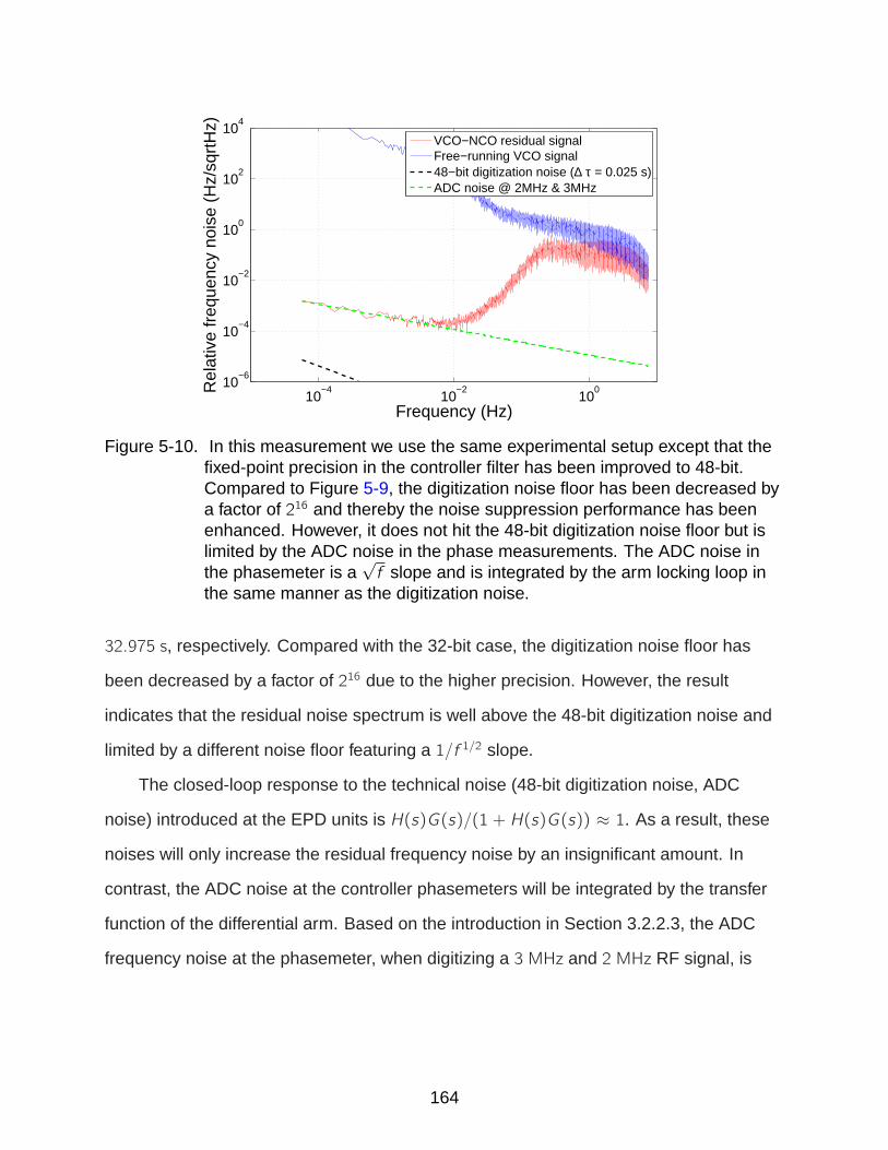
10−4
10−2
100
10−6
10−4
10−2
100
102
104
Frequency (Hz)
Rel
ativ
e fr
eque
ncy
nois
e (H
z/sq
rtH
z)
VCO−NCO residual signalFree−running VCO signal48−bit digitization noise (∆ τ = 0.025 s)ADC noise @ 2MHz & 3MHz
Figure 5-10. In this measurement we use the same experimental setup except that thefixed-point precision in the controller filter has been improved to 48-bit.Compared to Figure 5-9, the digitization noise floor has been decreased bya factor of 216 and thereby the noise suppression performance has beenenhanced. However, it does not hit the 48-bit digitization noise floor but islimited by the ADC noise in the phase measurements. The ADC noise inthe phasemeter is a
√f slope and is integrated by the arm locking loop in
the same manner as the digitization noise.
32.975 s, respectively. Compared with the 32-bit case, the digitization noise floor has
been decreased by a factor of 216 due to the higher precision. However, the result
indicates that the residual noise spectrum is well above the 48-bit digitization noise and
limited by a different noise floor featuring a 1/f 1/2 slope.
The closed-loop response to the technical noise (48-bit digitization noise, ADC
noise) introduced at the EPD units is H(s)G(s)/(1 + H(s)G(s)) ≈ 1. As a result, these
noises will only increase the residual frequency noise by an insignificant amount. In
contrast, the ADC noise at the controller phasemeters will be integrated by the transfer
function of the differential arm. Based on the introduction in Section 3.2.2.3, the ADC
frequency noise at the phasemeter, when digitizing a 3 MHz and 2 MHz RF signal, is
164
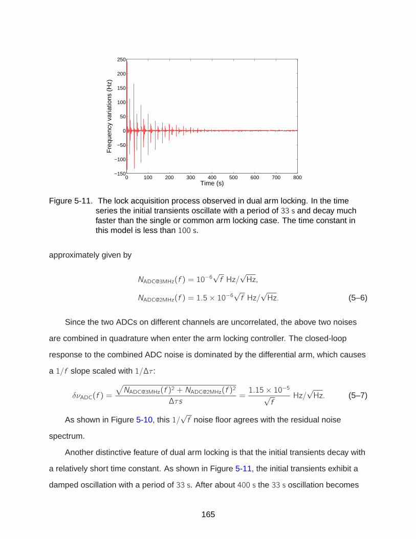
0 100 200 300 400 500 600 700 800−150
−100
−50
0
50
100
150
200
250
Time (s)
Fre
quen
cy v
aria
tions
(H
z)
Figure 5-11. The lock acquisition process observed in dual arm locking. In the timeseries the initial transients oscillate with a period of 33 s and decay muchfaster than the single or common arm locking case. The time constant inthis model is less than 100 s.
approximately given by
NADC@3MHz(f ) = 10−6√f Hz/
√Hz,
NADC@2MHz(f ) = 1.5× 10⁻⁶√f Hz/
√Hz. (5–6)
Since the two ADCs on different channels are uncorrelated, the above two noises
are combined in quadrature when enter the arm locking controller. The closed-loop
response to the combined ADC noise is dominated by the differential arm, which causes
a 1/f slope scaled with 1/∆τ :
δνADC(f ) =
√NADC@3MHz(f )2 + NADC@2MHz(f )2
∆τs=1.15× 10⁻⁵√
fHz/
√Hz. (5–7)
As shown in Figure 5-10, this 1/√f noise floor agrees with the residual noise
spectrum.
Another distinctive feature of dual arm locking is that the initial transients decay with
a relatively short time constant. As shown in Figure 5-11, the initial transients exhibit a
damped oscillation with a period of 33 s. After about 400 s the 33 s oscillation becomes
165

Figure 5-12. The experimental setup of frequency noise mitigation of the cavitystabilized laser using dual arm locking. The experimental principle is thesame as described in Figure 4-12, where the single arm locking sensor isreplaced with the dual arm locking sensor designed in the previous section.The averaged delay time between the two EPD units is realistic 33 s. Wemeasured the stabilized frequency noise of the RL− L2 beat signal withmultiple differential delay times.
invisible in the time series of the stabilized frequency, which is much shorter than the
required duration of more than ∼ 2000 s in single or common arm locking.
5.2.3 Integration with Pre-stabilized Laser
The application of dual arm locking on the frequency noise mitigation of pre-stabilized
lasers has been performed by means of an auxiliary phase-locked laser. This experiment
for the first time demonstrates that arm locking is capable of sufficiently reducing the
frequency noise of a cavity stabilized laser in the presence of realistic 33 s light travel
times. The experimental setup resembles the setup illustrated by Figure 4-12, while the
arm locking configuration has been expanded into two arms. As shown in Figure 5-12,
the frequency noise of L2 tracks the L1 as a phase-locking reference. The phase-locking
reference, which is driven by a NCO, is further phase-modulated via the dual arm
locking setup.
166
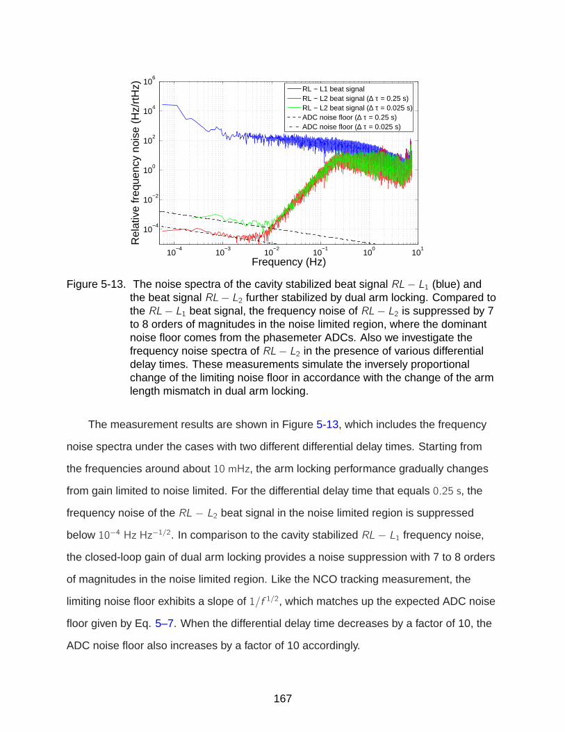
10−4
10−3
10−2
10−1
100
101
10−4
10−2
100
102
104
106
Frequency (Hz)
Rel
ativ
e fr
eque
ncy
nois
e (H
z/rt
Hz)
RL − L1 beat signalRL − L2 beat signal (∆ τ = 0.25 s)RL − L2 beat signal (∆ τ = 0.025 s)ADC noise floor (∆ τ = 0.25 s)ADC noise floor (∆ τ = 0.025 s)
Figure 5-13. The noise spectra of the cavity stabilized beat signal RL− L1 (blue) andthe beat signal RL− L2 further stabilized by dual arm locking. Compared tothe RL− L1 beat signal, the frequency noise of RL− L2 is suppressed by 7to 8 orders of magnitudes in the noise limited region, where the dominantnoise floor comes from the phasemeter ADCs. Also we investigate thefrequency noise spectra of RL− L2 in the presence of various differentialdelay times. These measurements simulate the inversely proportionalchange of the limiting noise floor in accordance with the change of the armlength mismatch in dual arm locking.
The measurement results are shown in Figure 5-13, which includes the frequency
noise spectra under the cases with two different differential delay times. Starting from
the frequencies around about 10 mHz, the arm locking performance gradually changes
from gain limited to noise limited. For the differential delay time that equals 0.25 s, the
frequency noise of the RL − L2 beat signal in the noise limited region is suppressed
below 10−4 Hz Hz−1/2. In comparison to the cavity stabilized RL − L1 frequency noise,
the closed-loop gain of dual arm locking provides a noise suppression with 7 to 8 orders
of magnitudes in the noise limited region. Like the NCO tracking measurement, the
limiting noise floor exhibits a slope of 1/f 1/2, which matches up the expected ADC noise
floor given by Eq. 5–7. When the differential delay time decreases by a factor of 10, the
ADC noise floor also increases by a factor of 10 accordingly.
167

Figure 5-14. The implementation of the modified dual arm locking sensor on UFLISexpands the original dual arm locking design by linearly combining thecommon arm and dual arm sensor signals. The low-pass filter FC(s) to bemultiplied with the common arm sensor is simplified into an integrator witha scaling factor of 1/τ . The high-pass filter FD(s) has a zero at DC and apole at around 1/τ ≈ 30 mHz to smooth the crossover between the twotransfer function. Note that the sampling frequency of FD(s) isdownsampled by a factor of 32 to maintain the open-loop stability.
5.3 Modified Dual Arm Locking
5.3.1 Modified Dual Arm Locking Sensor
As introduced in Section 2.3.3.3, the mapping vector of a modified dual arm
locking sensor consists of a low-pass filter FC(s) to amplify the common arm and a
high-pass filter FD(s) to suppress the differential arm at low frequencies. In spite of
the two additional filters, Figure 5-14 shows that the modified dual arm locking sensor
is designed in a similar way to the dual arm locking sensor. Our design follows the
simplified design described in Section 2.3.5, where the low-pass filter FC(s) is reduced
into an integrator with a scaling factor of 1/τ for the purpose of simplicity and efficiency.
The high-pass filter FD(s) has a zero at DC and a pole around 1/τ ≈ 30 mHz
to decrease the low frequency gain as well as to smooth the crossover between the
common arm and the dual arm.3 Compared with the data transfer rate of 488 kHz, the
3 In the specific design, the pole of FD(s) is actually at approximately 10 mHz tosmooth the crossover. Compared with Eq. 2–60, this will increase the noise limitations in
168

10−4
10−3
10−2
10−1
100
101
10−3
10−2
10−1
100
101
Mag
nitu
de
Frequency (Hz)
HD
(s)FD
(s)
P+(s)F
C(s)
10−5
10−4
10−3
10−2
10−1
100
101
10−1
100
101
Frequency (Hz)
Mag
nitu
de
measuredtheoretical
Figure 5-15. An example of a modified dual arm locking sensor with time delays of2.025 s and 1.975 s. (Left) The transfer function measurements of the dualarm and common arm components in the modified dual arm locking sensor.The originally flat magnitude response in the dual arm component is filteredby the high-pass filter FD(s) such that it starts to roll down with a s slope tozero at DC. The common arm component is multiplied by 1/s and scaled bythe factor of 1/τ . (Right) The combination of those two components yieldsthe overall transfer function of the modified dual arm locking sensor, wherethe overall magnitude response still retains flatness yet the common armnow dominates at low frequencies.
pole is at a significantly lower frequency such that the high-pass filter would be fairly
unstable with such a high sampling rate. 4 For this reason, the sampling frequency of
the high-pass filter is downsampled by a factor of 32 to maintain the open-loop stability.
The overall transfer function of the modified dual arm locking sensor is given by
HMD(s) =1
τsP+(s) + FD(s)HD(s). (5–8)
We measured the transfer function of the modified dual arm locking sensor and an
example with time delays of 2.025 s and 1.975 s is shown in Figure 5-15. The left figure
shows that the common arm dominates the frequencies below 1/τ and the dual arm
modified dual arm locking by a factor of about 3 and in the following analysis we need tokeep this factor in mind.
4 If we perform a z-transform to convert the filter with a 30 mHz corner frequency intothe z-domain using a sampling frequency of 488 kHz, the pole would be very close to theedge of the unit circle on the z-plane.
169

Figure 5-16. The preliminary experimental validation of the modified dual arm lockingsensor on UFLIS resembles the previous dual arm locking experiment. Themodified dual arm locking sensor extracts the instantaneous phaseinformation of the input laser noise and send it to the arm locking controller,which drives an 8 MHz NCO signal to track the 13 MHz laser beat note.The delay time on each arm is 33.025 s and 32.975 s, respectively.
dominates the frequencies above it. Their smooth crossover allows the shape of the
combined transfer function to be maintained flat in the LISA band.
5.3.2 Preliminary Test with NCO Tracking
The noise suppression performance of this modified dual arm locking sensor is
validated in a similar experiment setup with delay time 33.025 s and 32.975 s, as shown
in Figure 5-16. The input noise source is a 13 MHz beat signal between two Zerodur
cavity stabilized lasers RL and L1. The measurement results are shown in Figure 5-17.
Compared with the residual frequency noise spectrum obtained via dual arm locking
under the same arm length mismatch condition, the noise suppression performance has
been substantially improved to approximately 10−4 Hz Hz−1/2 at 3 mHz.
The enhancement in the noise suppression performance is attributed to the
mitigation of the noise limitations. Same as the experiment in the previous section,
the primary noise sources in this control system include the 48-bit digitization noise
inside the arm locking sensor/controller and the ADC noise at the phasemeters. The
noise amplitude is specified by Eq. 5–5 and Eq. 5–6, respectively. The frequency
170

10−4
10−2
100
10−6
10−4
10−2
100
102
104
Frequency (Hz)
Fre
quen
cy n
oise
(H
z/rt
Hz)
RL − L1 beat signalLaser − NCO beat signalADC noise floor − 0.025 s
Figure 5-17. The measurement result shows the modified dual arm locking significantlyimproved the noise suppression performance compared with the originaldual arm locking experiment. The 1/
√f slope ADC noise floor observed in
dual arm locking experiments has been surpassed. The final noiselimitation in a modified dual arm locking configuration, as described in Eq.5–9, is a combined effect of the digitization/ADC noise coupled in thecommon arm and in the differential arm.
response of the modified dual arm locking system to the input noise is described by Eq.
2–80, i.e.,
δνDig/ADC(f ) =H+
HMDNDig/ADC(f ) +
H−HMD
NDig/ADC(f ). (5–9)
Whether the common arm component or the differential arm component dominates
depends on the filter design and the arm length mismatch. In our setup the transfer
function of H+(s) and H−s is specified by Eq. 2–60. Under the condition of a 0.025 s
differential delay time, the magnitude responses are plotted in Figure 5-18. Due to
the simplified design of the filter FD(s) and the relatively short ∆τ , the differential arm
component dominates across the entire LISA band. Thus for frequencies below 10 mHz
(also the noise limited region), the ADC noise and the 48-bit digitization noise will be
amplified by the differential arm with a factor of 3 · τ /(2π∆τHMD(s)) ≈ 318, where the
factor of 3 comes from the pole frequency of FD(s) at 10 mHz. For frequencies well
171

10−4
10−3
10−2
10−1
100
10−1
100
101
102
103
Frequency (Hz)
Mag
nitu
de
H+(s)
H−(s)
1/(s*33s)
1/(s*0.025s)
Figure 5-18. The magnitude responses of H+(s) and H−(s) for the modified dual armlocking experiment. The expressions of H+(s) and H−(s) are specified byEq. 2–60, except that the pole of FD(s) is at 10 mHz rather than 30 mHz,causing the magnitude of H−(s) increases by a factor of 3 in the flat region.Due to the relatively short differential delay, the differential arm dominatesacross the entire LISA band.
below 1/τ , the dominant noise source is the proportionally scaled ADC noise floor,
which is given by
δνADC(f ) = NADC(f ) ·τ
2π∆τHMD= 5.73× 10⁻⁴
√f Hz Hz−1/2. (5–10)
In the noise limited region, the noise spectrum of the Laser-NCO beat signal is
consistent with the ADC noise floor given by Eq. 5–10. In this measurement we have
demonstrated that under the same condition of arm length mismatch, modified dual arm
locking has a better noise suppression performance than dual arm locking. Now that the
noise floor in the control system of our modified dual arm locking experiments has been
identified and verified quantitatively, we would expect the same noise floor when this
control system is applied onto the frequency noise mitigation of cavity stabilized lasers.
5.3.3 Integration with Pre-stabilized Laser
The incorporation of modified dual arm locking and a cavity stabilized laser
was experimentally demonstrated using the setup illustrated by Figure 5-19. The
172

Figure 5-19. Experimental setup of modified dual arm locking using an auxiliaryphase-locked laser. The experimental principle is the same as described inFigure 5-12, where the dual arm locking sensor is replaced with themodified dual arm locking sensor designed in the previous section. Theaveraged delay time between the two EPD units is 33 s and the differentialdelay time is 0.025 s (arm length mismatch ∼ 0.15%). We measured thestabilized frequency noise of the RL− L2 beat signal.
experimental setup is essentially the same as in Figure 5-12, where the frequency noise
of the RL − L1 beat signal is faithfully reproduced by the heterodyne phase-locked
RL− L2 beat signal. The frequency noise of RL− L2 can be therefore further suppressed
via the phase modulation from the arm locking feedback signal. The delay time on
each arm is 33.025 s and 32.975 s, respectively. The measurement results are shown
in Figure 5-20. In this measurement the frequency noise of the RL − L1 beat signal has
been suppressed by about 7 orders of magnitude at 3 mHz. The noise limited region
starts from ∼ 20 mHz, where the same ADC noise floor with a f 1/2 slope dominates the
frequency noise of the RL − L2 beat signal. The measured closed-loop transfer function
is consistent with the idealized model down to 20 mHz.
5.4 Arm locking Integrated With Far-end Phase-locking
Up to now we have characterized various arm locking configurations with LISA-like
delay time and Doppler shifts. We have also demonstrated the incorporation of arm
locking with cavity stabilization systems on our EPD-based electro-optical model and
173

10−4
10−2
100
10−6
10−4
10−2
100
102
104
Frequency (Hz)
Fre
quen
cy n
oise
(H
z/rt
Hz)
RL−L1 beat signalRL−L2 beat signal
10−4
10−2
100
10−8
10−6
10−4
10−2
100
102
Frequency (Hz)
Noi
se s
uppr
essi
on
idealizedmeasured
Figure 5-20. (Left) The noise spectra of the RL - L1 beat signal (blue) and the RL - L2beat signal (red). In this measurement we have achieved about 7 orders ofmagnitude noise suppression at 3 mHz. The noise limitation starting from∼ 10 mHz is the same ADC noise floor with a f 1/2 slope as seen in Figure5-17. The frequency noise from 0.1 Hz to 1 Hz is slightly above the0.3 Hz Hz−1/2 requirement, which can be alleviated by increasing theintegrator gain in that region. (Right) The measured transfer functionagrees with the idealized model very well down to about 10 mHz. Below10 mHz the control system becomes noise limited, which causes thedeviation from the idealized model.
achieved substantial noise suppression performance. In this section we take one
step forward to the aim of realistic arm locking hardware simulation by introducing the
transponder noise at far spacecraft. We will implement the phase-locked loop at the
far-end realistically rather than assume that the optical transponder functions perfectly
with an infinite feedback gain.
Moreover, in Section 2.3.5 we have derived that other realistic noise sources (clock
noise, spacecraft jitter, etc.) would couple into the stabilized laser noise in accordance
with the same transfer function as the transponder noise. Therefore, the transponder
noise limitation observed in the stabilized laser noise can be equivalently considered as
a manifestation of any additional noise source presented in arm locking. Our experiment
has for the first time demonstrated the arm locking performance in the presence of the
realistic transponder noise.
174

Table 5-1. Parameters in time-domain arm locking simulations with transponder noise
Parameter Symbol Value UnitsSampling frequency fs 10 Hz
Pre-stabilized frequency noise δν01 30×√1 + (2.8 mHz/f )4 Hz Hz−1/2
Free-running frequency noise δν02 10 kHz/f Hz Hz−1/2
Averaged delay time τ 33 sDifferential delay time ∆τ 0.025 sDoppler frequency error on arm 1-2 ∆ωD2 0 HzDoppler frequency error on arm 1-3 ∆ωD3 0 Hz
Transponder noise on arm 1-2 δν2PLL ∼ 10−2 · f Hz Hz−1/2
5.4.1 Transponder Noise Floor - Time Domain Simulation
The additional far-end PLL is nothing more than introducing an additional noise
source between the two delay lines, which can be either the transponder noise or any
other kind of realistic noise sources. The noise limitation derived from the transponder
noise is given by
δνtrans =H+
H(δνtrans2 + δνtrans3) +
H−H(δνtrans2 − δνtrans3), (5–11)
where the independent transponder noises on each arm, δνtrans2 and δνtrans3, are
uncorrelated. The common and difference noise between them yield the quadrature
sum, which is comparable to the transponder noise on a single arm. Therefore, we
could apply the additional transponder noise on only one arm without loss of quantitative
validity. For dual arm locking we have H+ = 1 and H− = 1/∆τs and for modified dual
arm locking we have H+ = FC + FD and H− = EFD/∆τs .
The verification of the transponder noise limitations was initially performed by
time-domain simulations using MATLAB SIMULINK packages. The software simulations
replicate LISA-like conditions as well as the sensor/controller design that have been
built in our benchtop experiments. The filters used in the time-domain simulation are
designed in the Laplace domain. Therefore, some deviation in the frequency response
between the software filters and the hardware filters should be expected. Tabel 5-1 lists
the parameters that are used in our simulations.
175

In the simulation the outgoing travel time and the return travel time are equal on
both arms, i.e., for ∆τ = 0.025 s we have τ12 = τ21 = 16.5125 s and τ13 = τ31 = 16.4875 s.
The Laplace domain filters, including E(s), FC(s), FD(s) and the f −1/2 controller filter,
have the same zeros and poles as their quantized z-domain counterparts in the
hardware implementation. Here we assume the transponder noise is a band-limited
blue noise (an f slope) in terms of frequency fluctuations. Note that this is just an
over-simplified model for the purpose of quick demonstration, while the realistic noise of
an analog PLL exhibits a f 1/5 slope in our measurement (see next section).
The simulation results are shown in Figure 5-21 using modified dual arm locking.
In this figure, the arm locking stabilized frequency noise is determined by three different
limitations: For frequencies above 0.1 Hz, the control system is gain limited and the
stabilized frequency noise agrees with the gain limited case without the transponder
noise. For frequencies below 0.1 Hz the noise suppression performance is limited by the
transponder noise floor, which is given by two segments: In the region from 30 mHz to
0.1 Hz, the transponder noise floor is dominated by the differential arm, which yields a
noise floor
δνTrans(f ) =10−2 · f2∆τs
= 3.2× 10⁻² Hz Hz−1/2. (5–12)
In a dual arm locking configuration this noise floor would dominate down through
lower frequencies. However for modified dual arm locking, for frequencies below 30 mHz
the high-pass filter FD effectively suppresses the magnitude of the differential arm, which
yields a noise floor with a lower magnitude:
δνTrans(f ) = 10−2f · τ
2 · 2π∆τ = 1.05 · f Hz Hz−1/2. (5–13)
The simulated frequency noise spectrum of the stabilized laser signal (the red
curve) agrees with the analytical limitations in all frequency regions. This simulation
numerically demonstrates that the transponder noise floor in a modified dual arm locking
configuration is less sensitive to the arm length mismatch.
176

10−4
10−3
10−2
10−1
100
101
10−8
10−6
10−4
10−2
100
102
104
Frequency (Hz)
Fre
quen
cy n
oise
(H
z/rt
Hz)
Pre−stabilized laser frequency noiseArm locking stabilized laser frequency noise (limited by open−loop gain)Transponder noise floor (δν(f) ⋅ 33/(2π ⋅ 0.025))Transponder noise floor (δν(f) ⋅ 1/s/0.025)Arm locking stabilized laser frequency noise (limited by transponder noise)
Figure 5-21. Time domain simulation of modified dual arm locking limited by thetransponder noise floor. The frequency noise of the stabilized laser (red) isdetermined by different mechanism in different frequency regions. Forfrequencies above 0.1 Hz the control system is gain limited and the redcurve follows the purple curve (the gain limited case). For frequenciesbetween 0.1 Hz and 30 mHz, the frequency noise of stabilized laser islimited by the transponder noise floor determined in dual arm locking (theyellow curve) with a transfer function of 1/s∆τ . For frequencies below0.1 Hz, the high-pass filter starts to suppress the magnitude of thedifferential arm sensor, which although still dominates through the rest ofthe measurement band. In this region the red curve follows the greencurve, which is given by the introduced transponder noise multiplied withthe differential arm gain of τ /(2π∆τ · HMD).
5.4.2 Experimental Verification - Simple Model
To simulate an additional noise source from far spacecraft on our hardware system,
we need to divide the delay time at the EPD units equally and delay the input electronic
signal using two split delay lines in cascade. Analogously, the arm length change due
to the LISA spacecraft motion is insignificant over a short time interval of 33 s, which
makes the outgoing time and the return time are almost the same. At the output of the
first delay line, the delayed signal can be used to phase-lock another laser that functions
177

Figure 5-22. Experimental setup of dual arm locking with function generator signal asthe transponder noise. In this setup the delay line on the arm 1-2 is equallydivided into two, representing the outgoing travel time τ12 and the returntravel time τ21. A function generator signal is used to demodulate the signaldelayed by τ12 such that the noise of the function generator signal entersthe entire round-trip delay line. It should be noted that in the phasemeasurement the frequency of the function generator signal has to beexactly accounted for to avoid the frequency pulling.
as a far spacecraft laser. Then the output signal of the phase-locked laser is sent to the
second delay line to generate the returning beam.
A simplified experimental verification of dual arm locking with the transponder noise
was performed using the NCO tracking configuration. Since the transponder noise can
be simplified into an arbitrary noise source entering between the outgoing delay and
the return delay, we use a function generator signal to simulate this additional noise
source. As shown in Figure 5-22, the delay line on the arm 1-2 is equally divided into
two delay times, representing the outgoing travel time τ12 and the return travel time τ21.
The Doppler shift frequency added to the nominal frequency of the “outgoing beam”
is +2 MHz, generating a 7 MHz Doppler-shifted signal. We place a function generator
producing a 3 MHz signal to demodulate the 7 MHz signal such that the noise of the
function generator signal enters the entire round-trip delay line via the analog mixer. It is
178

worth noting that like the local oscillator that drives the far-end phase-locking in realistic
LISA, the offset frequency of the function generator signal has to be taken into account
in the phase measurement of the long arm interferometry. That is, the function generator
has to be synchronized to the master clock and its nominal frequency has to match up
the corresponding 16-bit integer value (e.g., 3 MHz corresponds to 2.999305725 MHz)
to avoid generating an unwarranted Doppler frequency error. The demodulated 4 MHz
signal is then sent to the second delay line, which simulates the return beam being
transferred back to the local spacecraft.
The function generator noise is measured to be approximately 10−4 · f 3/4 Hz Hz1/2
via fractional delay filtering. With a differential delay time of 0.25 s and 0.025 s, the
expected transponder noise floor is given by 3.18 × 10⁻⁵f −1/4 Hz Hz−1/2 and 3.18 ×
10−4f −1/4 Hz Hz−1/2, respectively. We plot the measured residual frequency noise
spectrum in Figure 5-23. The measurements sufficiently demonstrate that in dual arm
locking the performance limitation due to the transponder noise inversely scales with
the arm length mismatch and the noise amplitude is consistent with our analytical
expectations.
5.4.3 Experimental Verification - Full Model
The complete experimental setup to verify the transponder noise floor in a modified
dual arm locking configuration is illustrated by Figure 5-24. In this setup we still use an
auxiliary phase-locked laser L2 to obtain the tunability of the pre-stabilization reference.
As the outgoing beam from the “local spacecraft”, the beat signal RL−L2 is electronically
split. Then the split signals travel to corresponding “far spacecraft” individually, which
is simulated by the EPD units. Similar to the simple model in the previous section,
we allocate the 33.025 s round-trip time equally into two delay lines, representing the
outgoing travel time τ12 and the return travel time τ21. Once the RL − L2 beat signal is
delayed by τ12 and arrives at the “far spacecraft”, its delayed and Doppler-shifted version
(a 3 MHz NCO signal) is used to heterodyne phase-lock a “far laser” represented by
179
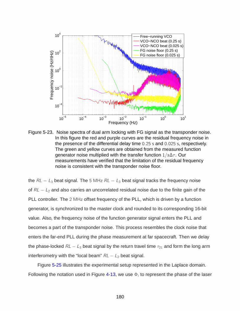
10−5
10−4
10−3
10−2
10−1
100
101
10−4
10−2
100
102
104
Frequency (Hz)
Fre
quen
cy n
oise
(H
z/rt
Hz)
Free−running VCOVCO−NCO beat (0.25 s)VCO−NCO beat (0.025 s)FG noise floor (0.25 s)FG noise floor (0.025 s)
Figure 5-23. Noise spectra of dual arm locking with FG signal as the transponder noise.In this figure the red and purple curves are the residual frequency noise inthe presence of the differential delay time 0.25 s and 0.025 s, respectively.The green and yellow curves are obtained from the measured functiongenerator noise multiplied with the transfer function 1/s∆τ . Ourmeasurements have verified that the limitation of the residual frequencynoise is consistent with the transponder noise floor.
the RL − L3 beat signal. The 5 MHz RL − L3 beat signal tracks the frequency noise
of RL − L2 and also carries an uncorrelated residual noise due to the finite gain of the
PLL controller. The 2 MHz offset frequency of the PLL, which is driven by a function
generator, is synchronized to the master clock and rounded to its corresponding 16-bit
value. Also, the frequency noise of the function generator signal enters the PLL and
becomes a part of the transponder noise. This process resembles the clock noise that
enters the far-end PLL during the phase measurement at far spacecraft. Then we delay
the phase-locked RL − L3 beat signal by the return travel time τ21 and form the long arm
interferometry with the “local beam” RL− L2 beat signal.
Figure 5-25 illustrates the experimental setup represented in the Laplace domain.
Following the notation used in Figure 4-13, we use Φi to represent the phase of the laser
180

Figure 5-24. Experimental setup of modified dual arm locking with far-end PLL. Thissetup exploits an auxiliary phase-locked laser L2 to obtain the tunability ofthe pre-stabilization reference. The delay line to simulate the LISA arm 1-2is divided equally into two, representing the outgoing and return travel timeindividually. Another beat signal RL− L3 is phase-locked to the RL− L2delayed by the outgoing travel time with an offset frequency of 2 MHz andthen delayed by the return travel time to have the heterodyne interferencewith the prompt beam. In this setup the function generator demodulatingthe heterodyne frequency of the PLL has an equivalent function as theclock on far spacecraft, where the clock noise enters the phasemeasurement of the far-end PLL in a similar way.
Li and an upper index of 0 to indicate the out-of-loop phase. In this diagram G0 is the
PLL gain for the phase-locking L2 to L1, while G1 and G2 follow the notation convention
to represent the arm locking gain and the PLL gain on the local spacecraft and the far
spacecraft, respectively. In the analysis we only consider the transponder noise as it is
the only dominant primary noise source in this setup and neglect any other secondary
noise including the digitization noise, the ADC noise, the lightpath noise, etc.
Identical to Eq. 4–6, the phase of the slave laser L2 is given by
Φ2 =1
1 + G0Φ02 +
G0
1 + G0(Φ1 + ϕNCO). (5–14)
181
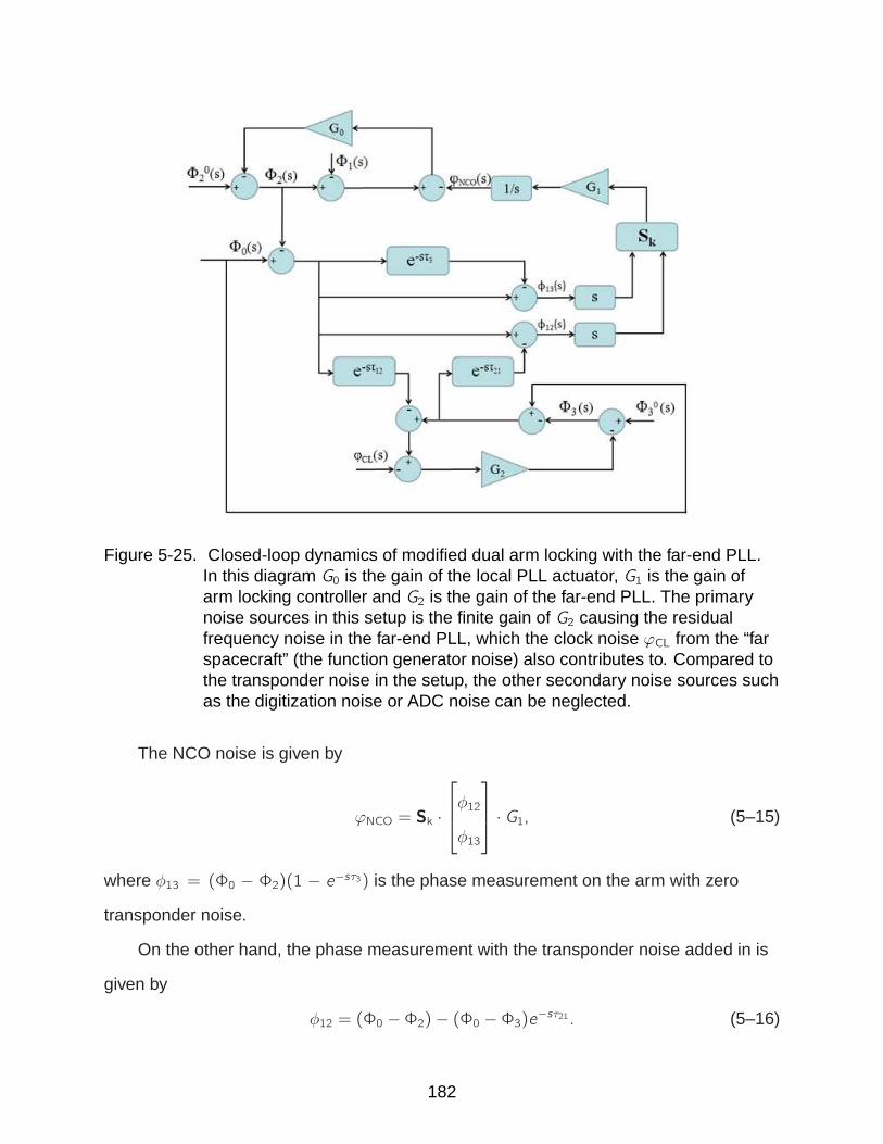
Figure 5-25. Closed-loop dynamics of modified dual arm locking with the far-end PLL.In this diagram G0 is the gain of the local PLL actuator, G1 is the gain ofarm locking controller and G2 is the gain of the far-end PLL. The primarynoise sources in this setup is the finite gain of G2 causing the residualfrequency noise in the far-end PLL, which the clock noise ϕCL from the “farspacecraft” (the function generator noise) also contributes to. Compared tothe transponder noise in the setup, the other secondary noise sources suchas the digitization noise or ADC noise can be neglected.
The NCO noise is given by
ϕNCO = Sk ·
φ12
φ13
· G1, (5–15)
where φ13 = (Φ0 − Φ2)(1 − e−sτ3) is the phase measurement on the arm with zero
transponder noise.
On the other hand, the phase measurement with the transponder noise added in is
given by
φ12 = (Φ0 −Φ2)− (Φ0 −Φ3)e−sτ21. (5–16)
182

Since the RL− L3 beat signal is phase-locked to the delayed RL− L2 beat signal, we
have
Φ0 −Φ3 =1
1 + G2(Φ0 −Φ03) +
G2
1 + G2
[(Φ0 −Φ2)e−sτ12 + ϕCL
], (5–17)
where ϕCL is the phase noise of the function generator that drives the PLL. Once the
function generator is synchronized to the master clock, it has an equivalent effect as the
clock noise from the far spacecraft SC2.
Substitute Eq. 5–17 into Eq. 5–16, we obtain the phase measurement on arm 1-2:
φ12 = (Φ0 −Φ2)−1
1 + G2(Φ0 −Φ03)−
G2
1 + G2
[(Φ0 −Φ2)e−sτ12 + ϕCL
]e−sτ21
=
(1− G2
1 + G2e−sτ2
)(Φ0 −Φ2)−
1
1 + G2(Φ0 −Φ03)e−sτ21 −
G2
1 + G2ϕCLe
−sτ21. (5–18)
The first term of Eq. 5–18 is the phase of the local beam multiplied by the transfer
function of the round-trip on arm 1-2. We define the transponder noise on arm 1-2:
δϕTrans =1
1 + G2(Φ0 −Φ03)e−sτ21 +
G2
1 + G2ϕCLe
−sτ21. (5–19)
Eq. 5–19 indicates that the transponder noise involves the intrinsic noise of the
far-end PLL due to the limited gain as well as the clock noise from far spacecraft.
For the purpose of symmetrical formalism, we also write the phase measurement
on arm 1-3 in the following form:
φ13 =
(1− G3
1 + G3e−sτ3
)(Φ0 −Φ2), (5–20)
where the PLL gain G3 is assumed to be infinite.
183
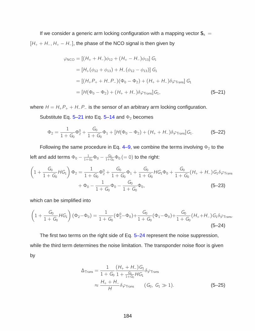
If we consider a generic arm locking configuration with a mapping vector Sk =
[H+ + H−,H+ − H−], the phase of the NCO signal is then given by
ϕNCO = [(H+ + H−)φ12 + (H+ − H−)φ13]G1
= [H+(φ12 + φ13) + H−(φ12 − φ13)]G1
= [(H+P+ + H−P−)(Φ0 −Φ2) + (H+ + H−)δϕTrans]G1
= [H(Φ0 −Φ2) + (H+ + H−)δϕTrans]G1, (5–21)
where H = H+P+ + H−P− is the sensor of an arbitrary arm locking configuration.
Substitute Eq. 5–21 into Eq. 5–14 and Φ2 becomes
Φ2 =1
1 + G0Φ02 +
G0
1 + G0Φ1 + [H(Φ0 −Φ2) + (H+ + H−)δϕTrans]G1. (5–22)
Following the same procedure in Eq. 4–9, we combine the terms involving Φ2 to the
left and add terms Φ0 − 11+G0Φ0 − G0
1+G0Φ0 (= 0) to the right:
(1 +
G0
1 + G0HG1
)Φ2 =
1
1 + G0Φ02 +
G0
1 + G0Φ1 +
G0
1 + G0HG1Φ0 +
G0
1 + G0(H+ + H−)G1δϕTrans
+Φ0 −1
1 + G0Φ0 −
G0
1 + G0Φ0, (5–23)
which can be simplified into
(1 +
G0
1 + G0HG1
)(Φ2−Φ0) =
1
1 + G0(Φ02−Φ0)+
G0
1 + G0(Φ1−Φ0)+
G0
1 + G0(H++H−)G1δϕTrans.
(5–24)
The first two terms on the right side of Eq. 5–24 represent the noise suppression,
while the third term determines the noise limitation. The transponder noise floor is given
by
∆Trans =1
1 + G0
(H+ + H−)G1
1 + G01+G0HG1
δϕTrans
≈ H+ + H−H
δϕTrans (G0, G1 ≫ 1). (5–25)
184

10−4
10−3
10−2
10−1
100
10−6
10−5
10−4
10−3
10−2
10−1
100
Frequency (Hz)
Fre
quen
cy n
oise
(H
z/rt
Hz)
Phase−locked loop noiseFunction generator noiseCombined transponder noise
Figure 5-26. Noise spectra of the transponder noise observed in modified dual armlocking. The measurement has identified that the primary contribution tothe transponder noise comes from the gain limited PLL and the functiongenerator noise is well below it.
The result of Eq. 5–25 is consistent with Eq. 5–11, proving the validity of this
experimental setup to demonstrate the transponder noise floor.
With a certain controller gain, the transponder noise is measured to be approximately
a 3 × 10⁻⁴ f 1/5 Hz Hz−1/2 slope, as shown in Figure 5-26. The primary contribution in
the transponder noise comes from the phase-locked loop, while the function generator
noise is much lower. As the PLL gain decreases, the transponder noise amplitude will
proportionally increase.
The measurement results are illustrated in Figure 5-27. As the differential delay
time equals 0.025 s, the expected transponder noise floor below 30 mHz is approximately
given by 0.20 f 1/5 Hz Hz−1/2, which limits the noise suppression performance in that
region. Our measurement has originally demonstrated that the arm locking stabilized
frequency noise agrees with this expected noise floor and still sufficiently meet the LISA
requirement in the presence of transponder noise. For frequencies around 30 mHz
the arm locking performance is still gain limited and the transponder noise floor given
185

10−4
10−3
10−2
10−1
100
101
10−4
10−2
100
102
104
Frequency (Hz)
Fre
quen
cy n
oise
(H
z/rt
Hz)
RL − L1 beat signalRL − L2 beat signal Transponder noise floorRL − L2 beat signal (lower PLL gain)RL − L2 beat signal (higher PLL gain)
Figure 5-27. Noise spectra of the stabilized laser frequency and the transponder noisefloor. In this figure the stabilized frequency noise is represented by the redcurve, which is limited by the transponder noise floor . The yellow curverepresent the transponder noise floor given by the combined noise inFigure 5-26 multiplied with the differential arm gain of τ /(2π∆τ · HMD). Thered and yellow curves agree with each other in the noise limited region.Note that the far-end PLL was set to gain limited such that the amplitude ofthe PLL noise can be continuously manipulated by adjusting the loop gain.As the PLL noise increases or decreases, the transponder noise floor in thestabilized laser frequency also tracks this change, which is shown by thegreen (a higher PLL gain) and purple (a lower PLL gain) curves.
by 1/∆τs is still below the RL − L2 frequency noise. We also have demonstrated that
as the PLL gain changes, the corresponding transponder noise will track the change
accordingly within a certain range. The measurements indicate that the transponder
noise floor inversely scales with the PLL gain as expected.
186

CHAPTER 6DOPPLER FREQUENCY ERROR IN ARM LOCKING
In this chapter we will investigate the impact of Doppler frequency errors on arm
locking. The research of Doppler frequency errors can be divided into two categories:
The on-board estimation of Doppler frequency errors and the techniques to restrict
the induced frequency pulling. In realistic LISA, the Doppler shift frequency is a
time-variable quantity due to the changing relative velocity between spacecraft.
Therefore, the initial Doppler frequency, as well as its first time derivative will be
estimated. The error in this estimation will cause a Doppler frequency error in the phase
measurements on the local spacecraft. Since the estimated Doppler frequency will not
be updated while arm locking is in operation, the consequent Doppler frequency error is
also a function of time. In this chapter we will focus more on the frequency pulling and
associated remedy schemes, rather than the simulation of Doppler frequency errors.
Note that the Doppler-induced frequency pulling also includes the situations in lock
acquisition and in the steady state, and here we primarily investigate the latter situation
as it has a long-term effect on the laser frequency.
6.1 Doppler Frequency Error in LISA
The LISA orbits are designed to have a 1-year period oscillations of the arm
lengths, interior angles and relative velocities, which means the Doppler frequency
variation also oscillates with a 1-year period. Therefore, the Doppler frequency
corresponds to an oscillation at 3.17 × 10⁻⁸ Hz. Since the relative velocity between
spacecraft can reach up to vSC = 18 m/s, the corresponding round-trip Doppler shift
frequency νD to the laser frequency ν0 yields the relation
νDν0=vSC
c. (6–1)
Thus the Doppler frequency can be up to approximately 17 MHz. As this frequency
is estimated and then subtracted in the phase measurements, a Doppler frequency error
187

will show up in the phase data and eventually drive the frequency of the master laser. In
realistic LISA, the Doppler frequency as well as its time derivatives (the Doppler change
rate) will be initially measured and then subtracted before arm locking is engaged. The
estimation of the Doppler frequency νD can be realized by various techniques: For
example, the on-board ranging can measure the relative velocity between the spacecraft
or the averaged laser beat frequency allows to estimate the Doppler frequency directly
by comparing the incoming beat frequency and the outgoing beat frequency.
However, how large the Doppler frequency error ∆νD will be is still uncertain. If we
expand the time-varying Doppler frequency error to the second order of time derivative
in the time domain and assume that the Doppler change rate (the first and second
derivatives) are constant as the variation is very small, the Doppler frequency error ∆νD
as a function of time is given by
∆νD(t) ≈ ∆νD0 + ∆νDt +1
2∆νDt
2. (6–2)
The performance of Doppler estimations depends on the initial laser frequency
noise ν0(f ) before arm locking and the estimation duration time T , yet is independent
of arm locking configurations, provided that the round-trip travel time τ is constantly
33 s. In the initial phase measurement, the contribution to the variance of the measured
frequency, σ2, primarily comes from the Doppler frequency error. Thus they can be
considered as equivalent to each other. According to Ref [13], the variance is given by
σ2 = 4
∫ ∞
0
df ν0(f )2sinc2(fT ) sin2(πf τ), (6–3)
where the sinc function comes from the Laplace transform of the averaging time T and
the sin function comes from the interferometer response on one arm.
For an averaging estimation time of 100 s, the initial Doppler frequency error
would be approximately 400 Hz with a Mach-Zehnder pre-stabilized laser; while for a
free-running laser the error could be as high as ∼ 105 Hz.
188

Once the arm locking is engaged, the Doppler frequency error will enter the
controller which causes the laser frequency to ramp. During this lock acquisition
process, the Doppler frequency error could generate a relatively large initial transient
(several hundred MHz) imposed onto the laser frequency, which is given by the product
of the error and the step response of the control system. When arm locking enters its
steady state, the Doppler frequency estimations will not be updated until the next time
the arm locking loop is needed to be unlocked (e.g., when changing the heterodyne
frequency or switching the arm locking configuration). After days or months, the Doppler
frequency estimations will be made very accurate due to the long averaging time and
thereby the initial transients occurring in lock acquisition will be significantly smaller than
the first time.
Thus in the steady state, the residual Doppler frequency error primarily comes from
the time-varying Doppler frequency that tracks the orbital motion of LISA spacecraft.
Depending on different arm locking configurations, the frequency pulling rate is derived
in Section 2.3.3. The expected frequency pulling in the steady state is limited within
10 MHz peak to peak, which is even less significant than the intrinsic drift of the laser
frequency, provided that the arm locking configuration can be exploited appropriately
based on the arm length mismatch.
6.2 Investigation of Frequency Pulling on UFLIS
In this section we will study the Doppler-induced frequency pulling rate in the steady
state, in the presence of various arm locking configurations. So far, all of the arm locking
benchtop experiments simulated an ideal situation without any Doppler shift or when
the Doppler frequency was perfectly accounted for in the phase measurements. In the
following time-domain simulations and benchtop experiments [95], we will generate
constant and step Doppler frequency errors in phase measurements, which is adequate
to observe the frequency pulling in the steady state. We will also use the modified dual
189

arm locking sensor to experimentally demonstrate its capability to concisely reduce the
frequency pulling rate.
In addition to the modified dual arm locking sensor, an AC-coupled controller with its
magnitude suppressed below the LISA band is also capable of reducing the frequency
pulling rate. Such a low frequency filtering mechanism can still be included in the arm
locking controller design as an additional constraint, even if a modified dual arm locking
sensor is used. The advantage is that it can further reduce the residual frequency
pulling rate and ensure the frequency pulling rate will never reach too high in case
the system is switched to other arm locking configurations. However, an AC-coupled
controller may bring a limitation to the achievable gain, which makes the control system
of arm locking gain limited when the arm length mismatch is large. Also, the phase
margin at the zero-crossing below the LISA band needs to be carefully retained for the
purpose of the closed-loop stability. Both of the two issues require a deliberate controller
design.
6.2.1 Generation of Doppler Frequency Errors
Since the Doppler shift frequency generated by current EPD units is a constant
value and cannot be continuously tuned, the Doppler frequency error can only be
generated as a constant. In Chapter 3 we already mentioned that the phasemeter offset
frequency is a 16-bit fixed-point integer number while the Doppler frequency specified
on the motherboard is a floating-point number. And to perfectly account for the Doppler
frequency, we rounded the floating-point Doppler frequency to the corresponding 16-bit
integer value. Therefore, if we generate the Doppler frequency error by changing the
phasemeter offset frequency, it can only be discretely introduced with a frequency
resolution 62.5 MHz/216 ≈ 954 Hz. With such a large Doppler error, the arm locking
filters would be required to have a much larger dynamic range to track the fast frequency
pulling. To generate a smaller Doppler frequency error, we have to decrease the
frequency resolution by increasing the precision of the phasemeter offset frequency.
190

In comparison, the EPD delay line is more flexible to change for the generation of a
Doppler frequency error with essentially an arbitrary value. Currently, a constant Doppler
frequency error can be simulated in three simple ways on UFLIS:
1. Directly modify the Doppler frequency value in the C program by adding anadditional constant to the original 16-bit number such that the Doppler frequencyerror is given by the constant. The advantage of this method is that a LISA-liketime-varying Doppler frequency can also be simulated based on this method,where the additional value becomes a frequency modulation with a 1-year period.
2. Change the clock frequency for the EPD unit. Since in the EPD unit the Dopplerfrequency scales with the clock frequency of 62.5 MHz, the Doppler frequencyerror δνD is given by (∆fclock/fclock) · νD. This method is straightforward as neithersoftware or hardware is needed to be modified. Also if we apply a frequencymodulation on the clock frequency, a time-varying Doppler frequency is essentiallyachievable. However, the frequency of the frequency modulation cannot be madeas low as 10−8 Hz due to the hardware limit. Another issue of this method is thatthe Doppler frequency error generated on two arms become correlated.
3. Use the setup illustrated by Figure 5-22, where the Doppler shift frequency isapplied in the middle of two delay lines. The signal source to provide the Dopplerfrequency, such as a function generator, is suggested to be synchronized to themaster clock (though not required in this situation). Similar to the second method,a time-varying Doppler frequency can also be realized by frequency-modulatingthe signal frequency, although the period of the frequency modulation is limited bythe parameter of the function generator.
In the following experiments we mainly employ Method 2 and 3.
6.2.2 Frequency Pulling in Single Arm Locking
In this section we will first discuss a pioneering experiment in which a constant
Doppler error is introduced into our single arm locking loop and a designed AC-coupled
controller is dedicated to eliminate the frequency pulling. Figure 6-1 illustrates the
experimental configuration, in which a 6 MHz free running VCO signal is demodulated
with a 9 MHz NCO signal. The beat signal of 3 MHz is then split into a prompt signal
and a signal which is delayed by 1 s as well as shifted by 4 MHz. The phasemeter will
demodulate the error signal with an 16-bit offset frequency.
191

Figure 6-1. The preliminary experimental setup of AC-coupled single arm locking withDoppler error. A 5 Hz constant Doppler frequency error is generated byshifting the clock frequency of the EPD unit by 80 Hz. The clocks that drivethe EPD unit and the arm locking controller are synchronized to accuratelycontrol the Doppler frequency. An AC-coupled controller with a flatmagnitude response at DC is used to eliminate the frequency pulling.
0 0.5 1 1.5 2 2.5 3 3.5 4
x 104
−2
−1.5
−1
−0.5
0
0.5
1x 10
4
Time (s)
Fre
quen
cy V
aria
tions
(H
z)
Free−running VCOStabilized VCO with AC−couplingStabilized VCO with DC−coupling
10−4
10−2
100
102
10−3
100
103
106
109
Frequency (Hz)
Pha
se N
oise
(cy
cles
/sqr
tHz)
Free−running VCOStabilized VCO with AC−couplingStabilized VCO with DC−coupling
Figure 6-2. (Left) Time series of a free-running VCO signal, a stabilized VCO signal withthe AC-coupled controller and a stabilized VCO signal with a standardDC-coupled controller. The AC-coupled controller is capable of removing thefrequency pulling that shows up in the situation with the DC-coupledcontroller. (Right) Linear spectral densities of the phase noise of the threetime series. Although the Doppler error does not cause frequency pullingwith the AC-coupled controller, the controller gain is significantly limited andthe noise suppression performance is compromised.
192

In the basic experiment described in Section 4.2, this offset frequency matches the
Doppler frequency perfectly, while here we introduce a constant Doppler frequency error
of 5 Hz by changing the clock frequency of the EPD unit. In the presence of a standard
DC-coupled controller, the frequency pulling rate is then given by νD/τ = 5 Hz/s,
which is demonstrated by the stabilized time series (the green curve in Figure 6-2
(left)). In contrast, the red curve represents the time series stabilized by an AC-coupled
controller. The time series of frequency fluctuations exhibit the frequency pulling in
lock acquisition, which is given by the convolution between the Doppler error and
the AC-coupled controller transfer function at low frequencies. Since the AC-coupled
controller is designed to have a constant low gain at DC, a constant frequency offset
(∼ 9 kHz) is added to the output frequency through the lock acquisition process. After
the initial frequency pulling is relaxed and the system enters the steady state, the
stabilized frequency stays flat and the residual frequency pulling rate is strictly zero.
Figure 6-2 (right) shows the linear spectral densities of the phase fluctuations of the
three beat signals. The DC-coupled controller has the best in-band performance but the
frequency is ramping down with the expected rate. Note that this AC-coupled controller
is just for the purpose of demonstration: We use a fairly high low unity gain frequency
compared to LISA to perform the measurement in a reasonable time. This limits the
noise suppression in our experiments compared to the noise suppression expected in
LISA.
6.2.3 Frequency Pulling in Dual and Modified Dual Arm Locking
6.2.3.1 Time-domain simulations with AC-coupled controll er
The Doppler impact becomes critical in a dual arm locking configuration when
the arm length mismatch is small. Here we represent a time-domain simulation of
an AC-coupled dual arm locking configuration with Doppler errors. This time-domain
simulation is running on a Matlab Simulink model with floating point arithmetic. In dual
arm locking the critical parameter is the differential Doppler frequency error between
193

Table 6-1. Parameters in AC-coupled dual arm locking simulations with Doppler errors
Parameter Symbol Value UnitsSampling frequency fs 10 Hz
Free-running frequency noise δν01 10 kHz/f Hz Hz−1/2
Average delay time τ 33 sDifferential delay time ∆τ 0.255 sDoppler frequency error on arm 1-2 ∆νD2 150 kHzDoppler frequency error on arm 1-3 ∆νD3 149 kHzLoop gain G0 100
Table 6-2. Parameters of the AC-coupled filter used in simulations
zeros (Hz) poles (Hz)10−7 5× 10−610−7 5× 10−610−6 3× 10−35× 10−5 3× 10−35× 10−5 3× 10−30.1 3× 10−30.3 3× 10⁻³
two arms, where a smaller arm length mismatch results in a smaller differential Doppler
error. In our simulation we assume a free-running laser with a large Doppler frequency
error on each arm, while the difference between them is 1 kHz. The parameters used
are list in Table 6-1 and the AC-coupled controller is designed with the zeros and poles
listed in Table 6-2.
The black curve in Figure 6-3 (right) is the open-loop transfer function which is given
by the dual arm locking sensor (the blue curve) multiplied by the AC-coupled controller
(the red curve) with a loop gain factor G0. The AC-coupled controller consists of a f −1/2
slope low-pass filter for the high frequency suppression and a high pass filter to reduce
the frequency pulling. The open-loop transfer function provides a bandwidth of around
42 kHz and a unity gain frequency of 15 µHz at low frequencies. The maximum of the
open-loop gain is approximately 100 dB at 3 mHz; then the gain starts to decrease with
a slope of f 2 due to the AC-coupling. Note that the slope of the AC-coupled filter at the
zero-crossing yields an s slope to avoid excessive phase shift.
194

0 2 4 6 8 10
x 105
−1.5
−1
−0.5
0
0.5
1x 10
6
Time (s)
Lase
r F
requ
ency
(H
z)
0.04841 Hz/s
10−8
10−6
10−4
10−2
100
−200
−150
−100
−50
0
50
100
150
200
Frequency (Hz)
Mag
nitu
de r
espo
nse
(dB
)
OLTF(s)G(s)G
eff(s)
Heff
(s)
H(s)TF
D+(s)
TFD−
(s)
Figure 6-3. (Left) Simulated time series of the output frequency change due to a 1 kHzDoppler error with an AC-coupled controller. (Right) Modeled frequencyresponses of a generic dual arm locking loop to common and differentialDoppler errors in the presence of an AC-coupled controller.
The frequency response to Doppler errors can be more easily explained by defining
an effective sensor Heff(s) = P−(s) and effective controller Geff(s) = G0G(s)/(∆τs)
in the differential path. In Figure 6-3 (right) the yellow curve and the cyan curve
demonstrate the effective controller Geff and the effective sensor Heff in the differential
arm respectively. The closed-loop frequency response to the differential Doppler error is
illustrated by the green curve in the figure. Depending on the gain level of the open-loop
transfer function Heff(s)Geff(s), the closed-loop frequency response consists of three
segments in different frequency regions:
TFD−(s) =
1Heff(s)
≈ 12∆τs, when f ≫ fUG
Geff(s)
1+Heff(s)Geff(s), when f ∼ fUG
Geff(s), when f ≪ fUG
(6–4)
where fUG is the lower UGF of the high pass filter.
We are more interested in the region where the closed-loop frequency response is
approximately equal to the effective controller, i.e., TFD−(s) = Geff(s) = G0G(s)/(∆τs).
The 1/s slope in the frequency response indicates a Doppler error induced pulling still
occurs in the output frequency. However, compared with the large gain factor of 1/(2∆τ)
in the DC-coupling situation, the gain factor now is significantly reduced due to the
195

low gain of the AC-coupled controller. If we recall that the gain factor of 1/s is directly
proportional to the drift rate of the frequency pulling, it is straightforward to derive the
reduced drift rate given by
(dνLdt
)
AC−coupled= 2G0G(s)
(dνLdt
)
DC−coupled. (6–5)
This relation indicates that the reduced drift rate is also directly proportional to
the loop gain. Our time-domain simulation is based on a long arm length mismatch of
2∆τ = 0.51 s and an inaccurate differential Doppler estimation of ∆νD− = 1 kHz. Without
the AC-coupling scheme the drift rate would be 1 kHz/0.51 s ≈ 1961 Hz/s for a high gain
DC-coupled controller. Figure 6-3 (left) shows the time series of the variation of the laser
frequency using our AC-coupled controller. The frequency pulling in lock acquisition
yields a maximal frequency offset of approximately 1.2 MHz. In the steady state the drift
rate has been reduced to 0.04841 Hz/s, which is exactly what we expect based on the
frequency domain analysis presented above. Note that we reduced the laser frequency
noise in this simulation to zero to be able to determine the drift rate with this accuracy.
6.2.3.2 Experiments with modified dual arm locking sensor
In the following experiments we will verify the frequency pulling rate of dual/modified
dual arm locking in the steady state. The experimental setup is illustrated by Figure
6-4, where the Doppler frequency errors are generated by shifting the clock frequency.
The block labeled with mapping vector represents the dual or modified dual arm locking
mapping vector designed in Chapter 5. The Doppler frequency errors generated in the
phase measurements are 6.4 Hz and 9.6 Hz, respectively. Therefore, with τ = 33 s and
∆τ = 0.025 s, the expected frequency pulling rates are
(dνLdt
)
Dual
=∆νD−2∆τ
= 64 Hz/s,
(dνLdt
)
ModifiedDual
=∆νD+2τ
= 0.24 Hz/s. (6–6)
196

Figure 6-4. Experimental setup of dual/modified dual arm locking with Dopplerfrequency errors, which are generated from the clock frequency offset of200 Hz. The Doppler frequency errors in the phase measurements are6.4 Hz and 9.6 Hz, respectively. The controller in this setup is still high-gainDC-coupled to observe the frequency pulling rate.
0 100 200 300 400 500 6000
0.5
1
1.5
2
2.5
3
3.5
4x 10
4
Time (s)
Fre
quen
cy fl
uctu
atio
n (H
z)
Modified dual arm locking (0.245 Hz/s)Dual arm locking(64.2 Hz/s)
Figure 6-5. Observed frequency pulling of dual/modified dual arm locking with Dopplerfrequency errors. For a dual arm locking and a modified dual arm lockingconfiguration, the observed frequency pulling rate is 64.2 Hz/s and0.245 Hz/s, respectively. These measurement results are consistent with thetheoretical predictions and demonstrate that the modified dual arm lockingsensor is capable of alleviating the Doppler issue substantially when the armlength mismatch is not very large.
197

0 500 1000 1500 2000 2500 3000 3500 4000−200
0
200
400
600
800
1000
Time (s)
Fre
quen
cy fl
uctu
atio
n (H
z)
Free−running frequency fluctuationsFrequency fluctuations stabilized by MDAL
10−4
10−3
10−2
10−1
100
101
10−4
10−2
100
102
104
Frequency (Hz)
Fre
quen
cy n
oise
(H
z/rt
Hz)
Free−running VCO noiseResidual noise stabilized by MDAL
Figure 6-6. (Left) The frequency fluctuations of the free-running VCO signal and theresidual signal stabilized by modified dual arm locking. Compared to thefrequency pulling of dual arm locking in Figure 6-5, where the stabilizedfrequency has been pulled by more than 35 kHz in 600 s, the modified dualarm locking sensor restricts the frequency pulling within a range of less than900 Hz in one hour. (Right) The noise spectra of the two time series. Herewe can see that the noise suppression performance is essentially notaffected by the frequency pulling after the linear drift is removed inpost-processing.
The observed frequency pulling for both two cases is shown in Figure 6-5. In a
duration of 600 s, the output frequency has drifted by more than 35 kHz when dual arm
locking is used. In contrast, the modified dual arm locking configuration limits the 1-hour
frequency pulling within a range of less than 900 Hz, as shown in Figure 6-6 (left). Note
that this frequency pulling rate is even smaller than a typical drift rate of cavity stabilized
lasers. From the frequency data we have obtained the frequency pulling rates are
64.2 Hz/s and 0.245 Hz/s. The measured frequency pulling rates match up the expected
values and has demonstrated that the modified dual arm locking sensor is capable of
alleviating the Doppler issue substantially when the arm length mismatch is not very
large. Figure 6-6 (right) shows the linear spectral density of the residual frequency
noise, which is essentially not affected by the linear frequency drift. 1
1 The LSD of the residual frequency noise is limited by precision loss in the E(s) filter,which is an old design, and is in any case independent of the frequency pulling rate.
198
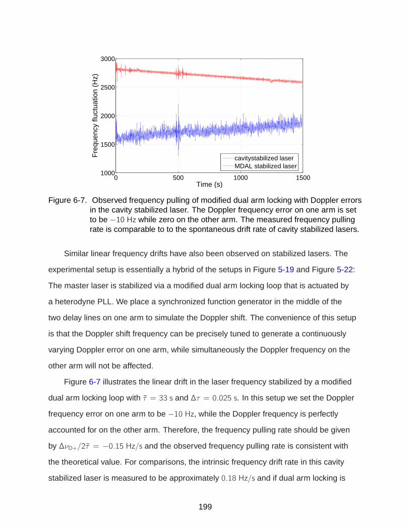
0 500 1000 15001000
1500
2000
2500
3000
Time (s)
Fre
quen
cy fl
uctu
atio
n (H
z)
cavitystabilized laserMDAL stabilized laser
Figure 6-7. Observed frequency pulling of modified dual arm locking with Doppler errorsin the cavity stabilized laser. The Doppler frequency error on one arm is setto be −10 Hz while zero on the other arm. The measured frequency pullingrate is comparable to to the spontaneous drift rate of cavity stabilized lasers.
Similar linear frequency drifts have also been observed on stabilized lasers. The
experimental setup is essentially a hybrid of the setups in Figure 5-19 and Figure 5-22:
The master laser is stabilized via a modified dual arm locking loop that is actuated by
a heterodyne PLL. We place a synchronized function generator in the middle of the
two delay lines on one arm to simulate the Doppler shift. The convenience of this setup
is that the Doppler shift frequency can be precisely tuned to generate a continuously
varying Doppler error on one arm, while simultaneously the Doppler frequency on the
other arm will not be affected.
Figure 6-7 illustrates the linear drift in the laser frequency stabilized by a modified
dual arm locking loop with τ = 33 s and ∆τ = 0.025 s. In this setup we set the Doppler
frequency error on one arm to be −10 Hz, while the Doppler frequency is perfectly
accounted for on the other arm. Therefore, the frequency pulling rate should be given
by ∆νD+/2τ = −0.15 Hz/s and the observed frequency pulling rate is consistent with
the theoretical value. For comparisons, the intrinsic frequency drift rate in this cavity
stabilized laser is measured to be approximately 0.18 Hz/s and if dual arm locking is
199

100 200 300 400 500 600 700 800 900−4000
−3000
−2000
−1000
0
1000
2000
Time (s)
Fre
quen
cy fl
uctu
atio
n (H
z)
cavity stabilizedMDAL stabilizedMDAL simulation
Figure 6-8. Observed frequency pulling in lock acquisition due to a step function inDoppler errors. After the step Doppler error enters the loop, the laserfrequency has been pulled by ∼ 3 kHz in lock acquisition and then drifts witha constant rate in the steady state. A time-domain simulation with the sameconditions was performed and the time series (the cyan curve) have shownconsistency with our measurements.
used, the frequency pulling rate would become −200 Hz/s. Our measurement has
demonstrated that modified dual arm locking is capable of reducing the frequency
pulling rate to a negligible level that is comparable to the spontaneous drift of cavity
stabilized lasers, provided that a reasonable Doppler estimation could be given.
In addition, we have also studied the responsive behavior of the stabilized laser
frequency to a step function in the Doppler error. Using the same experimental setup,
we start the arm locking loop without any Doppler error. After the laser frequency is
settled down, we initiate a step function in the Doppler frequency by 10 Hz and observe
the frequency pulling in the relock duration. The time series of the laser frequency is
shown in Figure 6-8, where we can see the laser frequency has been pulled by ∼ 3 kHz
and re-entered the steady state with a constant drift rate of −0.152 Hz/s in about 2 min.
200

To verify this lock acquisition process, we have run a time-domain simulation with the
same conditions and the result is given by the cyan curve in the figure. We can see that
in most regions the numerical simulation agrees with the measurement very well.2 The
deviation that happens during 350 s − 400 s is mainly ascribed to the difference in the
filter design between the simulation and hardware models, such as the error caused by
bilinear transform in the time-domain.
Still, to realistically simulate the time-variable Doppler frequency error, a simulator to
generate time-variable Doppler shift frequencies that track the spacecraft orbital motions
must be implemented on the EPD unit. However, an oscillation frequency of ∼ 10−8 Hz
is too low for laboratory experiments to effectively simulate. To circumvent this problem,
the plan is to rescale the orbital frequency of LISA and consequently the delay times,
as well as zeros and poles in arm locking filters, to a relatively short “lab-reasonable”
time scale, which requires the redesign of the entire arm locking system. Currently,
a new version of the EPD unit featuring such time-varying Doppler frequencies is in
development. Consequently, an adapted arm locking system will be built to study the
arm locking performance with realistic time-variable Doppler errors.
2 The time series of the stabilized laser frequency shows spurious peaks, which arehighly correlated to the unwarranted jumps in the input laser frequency. Our arm lockingloop is capable of attenuating frequency jumps within a range of ∼ 1 kHz.
201

CHAPTER 7CONCLUSION AND OUTLOOK
We tested different arm locking schemes for LISA using our LISA interferometer
testbed. The EPD-based electro-optical arm locking hardware simulations can
effectively and faithfully reproduce realistic LISA-like conditions such as 16 s light
travel time and variable MHz Doppler shifts, which are vital for the validity of arm locking
experiments. In particular, the dual and modified dual arm locking configurations are
linear combinations of LISA inter-spacecraft phase measurements optimized for the
noise performance and minimization of the Doppler-induced frequency pulling issue.
In this dissertation experimental verifications to examine them under realistic LISA-like
conditions are presented for the first time.
7.1 Control System of Arm Locking
On UFLIS we have implemented four basic arm locking configurations and
demonstrated their control system in a series of verification measurements. In our
experiments a laser beat signal with a heterodyne frequency in the range of 2 − 20 MHz
is received and converted into an electronic signal at the photodiode. The long arm
interferometer output is simulated via the analog mixing of the electronic signal and
its delayed replica. By demodulating the interferometer outputs, the phasemeters
extract the frequency fluctuations from each heterodyne beat signal. A dedicated
mapping vector is used to synthesize and manipulate the frequency fluctuations to
form an adequate linear combination, known as the error signal of arm locking. The
measurements have shown that the open-loop transfer functions of these arm locking
sensors agree very well with the theoretical design.
The arm locking controller on UFLIS was designed and built in parallel paths: A
compensator filter yields a 1/√f slope at frequencies above 1 Hz to alleviate the large
phase shift due to the round-trip delays. Four-stage cascaded integrators provide
sufficient noise suppressions in the LISA band. Through the combination of these two
202

control paths, a robust control system of arm locking have been achieved with both
a high bandwidth and a satisfactory noise suppression performance. Consequently,
we present the first ever experimental proof of these arm locking schemes in the
presence of realistic LISA-like long time delays and Doppler shifts, with unprecedented
noise suppression performances. In our experiments we achieved up to 6 orders of
magnitude noise suppression via single arm locking and up to 8 orders of magnitude via
dual/modified dual arm locking in the LISA band.
We also have studied the incorporation of arm locking with cavity stabilized lasers.
The combination of arm locking and the PDH stabilization technique will provide more
noise suppressions; however, it requires the reference of the PDH stabilization to be
frequency tunable. Therefore, we present a modification to the standard PDH setup
known as the PZT actuator, by which the resonant frequency of the cavity can be
adjusted in accordance with the arm locking feedback signal. We also present a second
method to introduce an auxiliary laser offset phase-locked to the master laser. The slave
laser reproduces the noise property of the master laser as well as obtains the frequency
tunability through the offset frequency of the local oscillator. These measurements have
demonstrated that arm locking can be easily reconciled with the cavity stabilization
without explicitly degrading the noise suppression performance of either of them.
7.2 Noise Limitations
Depending on scheme used and actual light travel times, arm locking can be gain
limited or limited by several external noise sources. The primary noise sources in arm
locking include clock noise, spacecraft motion, shot noise, technical noise and possibly
far-end PLL noise. In our experiments we analyzed the impact of various noise sources
on the noise suppression performance under different circumstances.
We also studied the influence of digitalization noise in the digital arm locking
sensors and controllers on the performance of arm locking. These results can be
used to design the digital arm locking system for LISA. The ADC noise in phase
203

measurements is another primary noise source that limits the arm locking performance
in our experiments. In realistic LISA the ADC noise performance in the phasemeter will
be optimized to meet the 1 pm Hz−1/2 requirement and should not cause a problem.
Nevertheless, our measurements have verified that the limiting ADC noise floor
is consistent with the theoretical predictions in the context of UFLIS. Moreover, by
investigating the ADC noise limitation we present the experimental proof that with the
same arm length mismatch, the noise performance of modified dual arm locking is
substantially superior to that of dual arm locking.
A more realistic demonstration of modified dual arm locking with the far-end
transponder noise is also presented in this dissertation. In the experiment we implemented
an analog phase-locked loop at the far-end to phase lock the local beat signal to the
incoming delayed signal. The transponder noise limitation observed in the stabilized
laser noise can be equivalently considered as a manifestation of any noise source
presented on the far spacecraft as they all couple into the arm locking control system in
the same fashion, i.e.,
δν =H+
H(δν2 + δν3) +
H−H(δν2 − δν3), (7–1)
where δνi , i = 2, 3 is any transponder noise introduced on the far spacecraft SC2, 3.
We measured the transponder noise limit in the stabilized laser and the PLL noise at the
far-end independently and found them in accordance with Eq. 7–1. The experiment also
reveals that in the presence of a non-negligible transponder noise and a relatively short
arm length mismatch (∆τ = 0.025 s), our modified dual arm locking configuration with
cavity stabilization still sufficiently meets the TDI capability with a margin of more than
25, 000 at 3 mHz.
7.3 Doppler-induced Frequency Pulling
The impact of Doppler shifts on arm locking was firstly identified from the arm
locking experiments on UFLIS and is a very critical issue that would ultimately affect
204

the feasibility of arm locking. More in-depth research on the Doppler impact gave a
better understanding of the Doppler frequency error, frequency pulling and helped
to identify solutions to overcome it. The arm locking control system implemented on
UFLIS provides an ideal environment to test the effects of frequency pulling and relevant
remedies.
By introducing a Doppler frequency error in the phase measurement, we have
demonstrated how the frequency pulling depends on different arm locking sensors.
These experiments are the first ever experimental proofs of arm locking in a realistic
and non-static LISA constellation. In particular, an AC-coupled controller for single
arm locking and dual arm locking has been developed in hardware and software
respectively, confirming that the frequency pulling can be substantially reduced or even
eliminated. We also compared the distinct frequency pulling rates of dual arm locking
and modified dual arm locking in response to same Doppler frequency errors. Our
experiment indicates that the modified dual arm locking sensor is capable of alleviating
the frequency pulling rate in the steady state to a negligible level, which is comparable to
the typical drift rate of a cavity stabilized laser.
We also have started the investigation of time-variable Doppler frequency errors in
hardware simulations. The observed frequency pulling in lock acquisition due to a step
function in the Doppler error agrees very well with the time domain simulation under the
same conditions.
7.4 Outlook
With the everlasting endeavor on gravitational wave detections in the past 50 years,
gravitational wave astronomy is expected to open a new window to the universe in this
decade, with the help of the next generation ground-based detectors, such as advanced
LIGO, VIRGO and LCGT, and the space-based project LISA. From gravitational
wave detections on compact binaries, black holes and Big Bang relics, entirely new
205

information on astrophysics and cosmology will be revealed and consequently extend
our understanding of the universe.
The low-frequency region that LISA will probe is full of interesting gravitational wave
sources, many of which still have never been seen. For coalescences of massive black
holes, as well as primordial gravitational waves generated in the extremely short time
after Big Bang, a space gravitational wave observatory such as LISA might be the only
accessible method to study them. LISA will precisely measure thousands of binary
systems in our Galaxy and yield new insights into the astrophysics of binary stars; LISA
will also provide a very first test of general relativity in extremely strong gravitational
fields on the vicinity of black holes by listening to the inspiral signals.
From the point of view of instrumentation, LISA is also a technically challenging
mission due to the required high sensitivity. The noise requirements for laser interferometry
and drag-free control are unprecedentedly stringent for current technology. The laser
frequency stabilization was once considered a difficult issue that may cause Time Delay
Interferometry to fail. Now multiple frequency control options have been proposed to
solve this problem and the selection is more based on the consideration of complexity,
cost, etc. Arm locking as one of the proposed laser frequency stabilization techniques,
entirely exploits LISA’s long arm interferometry to generate an error signal. This simple
architecture substantially saves on implementation resources. In addition, the integration
of arm locking and other pre-stabilization subsystems can suppress the laser frequency
noise below the pre-TDI requirement of 1 m ranging capability with an abundant margin,
which will further relax the dependence on ranging. The issue of Doppler-induced
frequency pulling slightly complicates the design of the control system of arm locking
and additional on-board data processing to estimate the Doppler frequency is needed.
Nevertheless, both analysis and experiments have shown that modified dual arm
locking solves this Doppler problem. We look forward a better understanding of LISA
technology, as well as a gravitational wave universe that LISA will ultimately discover.
206

REFERENCES
[1] A. Einstein. Gravitationswellen. Preussische Akademie der Wissenschaften,Sitzungsberichte, 1918:154–167, 1918.
[2] J. Weber. Detection and generation of gravitational waves. Phys. Rev., 117:306,1960.
[3] J. H. Taylor and J. M. Weisberg. A new test of general relativity - Gravitationalradiation and the binary pulsar PSR 1913+16. Astrophys. J., 253:908–920, 1982.
[4] J. M. Weisberg and J. H. Taylor. Observations of post-newtonian timing effects inthe binary pulsar psr 1913+16. Phys. Rev. Lett., 52:1348, 1984.
[5] B. F. Schutz. Gravitational wave astronomy. Class. Quantum Grav., 16:A131, 1999.
[6] D. Sigg et al. Status of the LIGO detectors. Class. Quantum Grav., 23:S51, 2006.
[7] P. Bender et al. LISA - Laser Interferometer Space Antenna for the detection andobservation of gravitational waves. MPQ-208, 1996.
[8] K. Danzmann et al. LISA - an ESA cornerstone mission for the detection andobservation of gravitational waves. Advances in Space Research, 32:1233, 2003.
[9] R. N. Lang and S. A. Hughes. Measuring coalescing massive binary black holeswith gravitational waves: the impact of spin-induced precession. Phys. Rev. D,74:122001, 2006.
[10] R. N. Lang and S. A. Hughes. Localizing coalescing massive black hole binarieswith gravitational waves. Astrophys. J., 677:1184, 2008.
[11] M. Tinto and J. W. Armstrong. Cancellation of laser noise in an unequal-arminterferometer detector of gravitational radiation. Phys. Rev. D, 59:102003, 1999.
[12] M. Tinto and S.L. Larson. The LISA zero-signal solution. Class. Quantum Grav.,22:S531, 2005.
[13] K. McKenzie, R. E. Spero, and D. A. Shaddock. Performance of arm locking inLISA. Phys. Rev. D, 80:102003, 2009.
[14] V. Wand et al. Implementation of arm locking with a delay of 1 second in thepresence of Doppler shifts. J. Phys.: Conf. Series, 154:012024, 2009.
[15] Y. Yu, S. Mitryk, and G Mueller. Experimental verification of dual/modified dual armlocking. Class. Quantum Grav., 28, 2011.
[16] C. Misner, K. Thorne, and J. Wheeler. Gravitation. W.H. Freeman and Company,San Francisco, CA, 1973.
207
[17] M. Maggiore. Gravitational Waves: Volume 1: Theory and Experiments. OxfordUniversity Press, 2007.
[18] K. Thorne. Gravitational waves. arXiv:gr-qc/9506086v1, 1995.
[19] J. W. T. Hessels, S. M. Ransom, I. H. Stairs, P. C. C. Freire, V. M. Kaspi, andF. Camilo. A radio pulsar spinning at 716 hz. science, 311:1901, 2006.
[20] L. Wang et al. The axisymmetric ejecta of supernova 1987a. Astrophys. J.,579:671, 2002.
[21] S. A. Hughes. Listening to the universe with gravitational-wave astronomy. AnnalsPhys., 303:142, 2003.
[22] R. F. Webbink. Watch this space: Observing merging white dwarfs.arXiv:1011.6317v1 [astro-ph.SR], 2010.
[23] A. Stroeer and A. Vecchio. The LISA verification binaries. Class. Quantum Grav.,23:S809, 2006.
[24] K. Belczynski, M. Benacquista, and T. Bulik. Double compact objects aslow-frequency gravitational wave sources. Astrophys. J., 725:816, 2010.
[25] G. Nelemans, S. F. P. Zwart, F. Verbunt, and L. R. Yungelson. Population synthesisfor double white dwarfs. A & A, 363:939, 2001.
[26] A. J. Ruiter, K. Belczynski, M. Benacquista, and K. Holley-Bockelmann. Thecontribution of halo white dwarf binaries to the Laser Interferometer Space Antennasignal. Astrophys. J., 693:383, 2009.
[27] Y. B. Zeldovich and I. D. Novikov. Soviet Physics Doklady, 9:246, 1964.
[28] E. F. Belland S. Phleps, R. S. Somerville, C. Wolf, A. Borch, and K. Meisenheimer.The merger rate of massive galaxies. Astrophys. J., 652:270, 2006.
[29] Flanagan and S. A. Hughes. Measuring gravitational waves from binary black holecoalescences. i. signal to noise for inspiral, merger, and ringdown. Phys. Rev. D,57:4535, 1998.
[30] Flanagan and S. A. Hughes. Measuring gravitational waves from binary black holecoalescences. i. signal to noise for inspiral, merger, and ringdown. Phys. Rev. D,57:4566, 1998.
[31] F. Pretorius. Evolution of binary black-hole spacetimes. Phys. Rev. Lett.,95:121101, 2005.
[32] M. Campanelli, C. O. Lousto, and Y. Zlochower. Last orbit of binary black holes.Phys. Rev. D, 73:061501, 2006.
208

[33] S. Chandrasekhar and S. Detweiler. The quasi-normal modes of the schwarzschildblack hole. Proc. R. Soc. Lond. A, 344:441, 1975.
[34] P. Amaro-Seoane, J. R. Gair, M. Freitag, M. C. Miller, I. Mandel, C. J. Cutler, andS. Babak. Intermediate and extreme mass-ratio inspirals - astrophysics, scienceapplications and detection using LISA. Class. Quantum Grav., 24:R113, 2007.
[35] J. R. Gair, L. Barack, T. Creighton, C. Cutler, S. L. Larson, E. S. Phinney, andM. Vallisneri. Event rate estimates for LISA extreme mass ratio capture sources.Class. Quantum Grav., 21:S1595, 2004.
[36] Stanislav Babak, Hua Fang, Jonathan R. Gair, Kostas Glampedakis, and Scott A.Hughes. “kludge” gravitational waveforms for a test-body orbiting a kerr black hole.Phys. Rev. D, 75:024005, 2007.
[37] C. Hopman and T. Alexander. The effect of mass segregation on gravitational wavesources near massive black holes. Astrophys. J. Lett., 645:L133, 2006.
[38] J. R. Gair and E. K. Porter. Cosmic swarms: a search for supermassive black holesin theLISA data stream with a hybrid evolutionary algorithm. Class. Quantum Grav.,26:225004, 2009.
[39] L. Barack and C. Cutler. LISA capture sources: Approximate waveforms,signal-to-noise ratios, and parameter estimation accuracy. Phys. Rev. D,69:082005, 2004.
[40] M. Hueller, M. Armano, L. Carbone, A. Cavalleri, R. Dolesi, C. D. Hoyle, S. Vitale,and W. J. Weber. Measuring the LISA test mass magnetic properties with a torsionpendulum. Class. Quantum Grav., 22:S521, 2005.
[41] S. A. Teukolsky. Perturbations of a rotating black hole. i. fundamental equationsfor gravitational, electromagnetic, and neutrino-field perturbations. Astrophys. J.,185:635, 1973.
[42] L. M. Krauss and M. White. Grand unification, gravitational waves, and the cosmicmicrowave background anisotropy. Phys. Rev. Lett., 69:869, 1992.
[43] R. Brustein, M. Gasperinib, M. Giovanninib, and G. Veneziano. Relic gravitationalwaves from string cosmology. Phys. Lett. B, 361:45, 1995.
[44] A. Buonanno, M. Maggiore, and C. Ungarelli. Spectrum of relic gravitational wavesin string cosmology. Phys. Rev. D, 55:3330, 1997.
[45] E. Witten. Cosmic separation of phases. Phys. Rev. D, 30:272, 1984.
[46] M. Kamionkowski, A. Kosowsky, and M. S. Turner. Gravitational radiation fromfirst-order phase transitions. Phys. Rev. D, 49:2837, 1994.
209
[47] T. Vachaspati and A. Vilenkin. Gravitational radiation from cosmic strings. Phys.Rev. D, 31:3052, 1985.
[48] D. Blair. The Detection of Gravitational Waves. Cambridge University Press, 2005.
[49] M. Tinto. Spacecraft doppler tracking as a xylophone detector of gravitationalradiation. Phys. Rev. D, 53:5354, 1996.
[50] F. Jenet, A. Lommen, S. Larson, and L. Wen. Constraining the properties ofsupermassive black hole systems using pulsar timing: an application to 3c 66b.Astrophys. J., 606:799, 2004.
[51] F. Jenet, G. Hobbs, K. Lee, and R. Manchester. Detecting the stochasticgravitational wave background using pulsar timing. Astrophys. J., 625:L123,2005.
[52] F. Acernese et al. The status of VIRGO. Class. Quantum Grav., 23:S63, 2006.
[53] B. Willke et al. GEO600: status and plans. Class. Quantum Grav., 24:S389, 2007.
[54] M. Ando et al. Current status of TAMA. Class. Quantum Grav., 19:1409, 2002.
[55] K. Kuroda and the LCGT Collaboration. The status of LCGT. Class. QuantumGrav., 23:S215, 2006.
[56] D. Shoemaker et al. Ground-based interferometric gravitational-wave detectors inthe LISA epoch. Class. Quantum Grav., 20:S11, 2003.
[57] S. Kawamura et al. The Japanese space gravitational wave antenna - DECIGO. J.Phys.: Conf. Ser., 122:012006, 2008.
[58] T. Prince and K. Danzmann. LISA science requirement document version 4.1. LISAInternational Science Team documentation, 2007.
[59] D. Shaddock, B. Ware, P. Halverson, R.E. Spero, and B. Klipstein. Overview of theLISA phasemeter. JPL Technical Report, 2006.
[60] T. Prince et al. LISA: Unveiling a hidden universe: Assessment study report.European Space Agency documentation, 2011.
[61] S. L. Larson, W. A. Hiscock, and R. W. Hellings. Sensitivity curves for spacebornegravitational wave interferometers. Phys. Rev. D, 62:062001, 2000.
[62] R. Dolesi et al. Gravitational sensor for LISA and its technology demonstrationmission. Class. Quantum Grav., 20:S99–108, 2003.
[63] W. J. Weber et al. Position sensors for LISA drag-free control. Class. QuantumGrav., 19:1751–6, 2002.
210

[64] L. Carbone et al. Achieving geodetic motion for LISA test masses: ground testingresults. Phys. Rev. Lett., 91:151101, 2003.
[65] D. W. Budworth, F. E. Hoare, and J. Preston. The thermal and magnetic propertiesof some transition element alloys. Proc. R. Soc. A, 257:250–62, 1960.
[66] Z. Silvestri et al. Volume magnetic susceptibility of gold-platinum alloys: possiblematerials to make mass standards for the watt balance experiment. Metrologia,40:172–6, 2003.
[67] P. McNamara et al. LISA Pathfinder. Class. Quantum Grav., 25:114034, 2008.
[68] G. Heinzel, C. Braxmaier, R. Schilling, A. Rudiger, D. Robertson, M. Plate, V. Wand,K. Arai, U. Johann, and K Danzmann. Interferometry for the LISA technologypackage (LTP) aboard SMART-2. Class. Quantum Grav., 20:S153, 2008.
[69] O. Jennrich. LISA technology and instrumentation. Class. Quantum Grav.,26:153001, 2009.
[70] M. Tinto, F. B. Estabrook, and J. W. Armstrong. Time-delay interferometry for LISA.Phys. Rev. D, 65:082003, 2002.
[71] D. A. Shaddock, B. Ware, R. E. Spero, and M. Vallisneri. Post-process time delayinterferometry for LISA. Phys. Rev. D, 70:081101, 2004.
[72] D. A. Shaddock et al. LISA frequency control white paper. LISA Project technicalnote LISA-JPL-TN-823, 2009.
[73] J. W. Armstrong, F. B. Estabrook, and M. Tinto. Time-delay interferometry forspace-based gravitational wave searches. Astrophys. J., 527:814–26, 1999.
[74] D. A. Shaddock et al. Data combinations accounting for LISA spacecraft motions.Phys. Rev. D, 68:061303, 1999.
[75] D. A. Shaddock. Operating LISA as a Sagnac interferometer. Phys. Rev. D,69:022001, 2004.
[76] V. Leonhardt and J. B. Camp. Space interferometry application of laser frequencystabilization with molecular iodine. Appl. Optics, 45:4142, 2006.
[77] R. W. P. Drever, J. L. Hall, F. V. Kowalski, J. Hough, G. M. Ford, and A. J. Munley.Laser phase and frequency stabilization using an optical resonator. Appl. Phys. B,31:97–105, 1983.
[78] G. Mueller G, P. McNamara P, J. I. Thorpe, and J. Camp. Laser frequencystabilization for LISA. Technical Report NASA/TM-2005-212794, 2005.
[79] F. Steier, F. C. Guzman, A. F. M. Garcia, D. Gerardi, G. Heinzel, and K. Danzmann.The end-to-end testbed of the optical metrology system on-board LISA pathfinder.Class. Quantum Grav., 26:094010, 2009.
211

[80] E. D. Black. An introduction to pound-drever-hall laser frequency stabilization. Am.J. Phys., 69:79–87, 2001.
[81] G. Heinzel et al. The LTP interferometer and phasemeter. Class. Quantum Grav.,21:S581–7, 2004.
[82] V. Wand et al. Noise sources in the LTP heterodyne interferometer. Class. QuantumGrav., 23:S159, 2006.
[83] J. Eichholz et al. Heterodyne laser frequency stabilization for the LaserInterferometer Space Antenna. accepted by J. Phys.: Conf. Series, 2011.
[84] B. S. Sheard, M. B. Gray, D. E. McClelland, and D. A. Shaddock. Laser frequencystabilization by locking to a LISA arm. Phys. Lett. A, 320:9, 2003.
[85] A. Sutton and D. A. Shaddock. Laser frequency stabilization by dual arm locking forLISA. Phys. Rev. D, 78:082001, 2008.
[86] M. Tinto and M. Rakhmanov. On the laser frequency stabilization by locking to aLISA arm. gr-qc/0408076, 2004.
[87] J. Sylvestre. Simulations of laser locking to a LISA arm. Phys. Rev. D, 70:102002,2004.
[88] M. Herz. Active laser frequency stabilization and resolution enhancement ofinterferometers for the measurement of gravitational waves in space. Opt. Eng.,44:090505, 2005.
[89] A. Marin et al. Phase locking to a LISA arm: first results on a hardware model.Class. Quantum Grav., 22:S235, 2005.
[90] Glenn de Vine et al. Experimental demonstration of Time-delay Interferometry forthe Laser Interferometer Space Antenna. Phys. Rev. Lett., 104:211103, 2010.
[91] J. I. Thorpe, R. J. Cruz, S. Sankar, and G. Mueller. Electronic phase delay - a firststep towards a bench-top model of LISA. Class. Quantum Grav., 22:S227–34,2005.
[92] S. Mitryk, V. Wand, and G Mueller. Verification of time-delay interferometrytechniques using the University of Florida LISA interferometry simulator. Class.Quantum Grav., 27:084012, 2010.
[93] J. I. Thorpe and G. Mueller. Experimental verification of arm-locking for LISA usingelectronic phase delay. Phys. Lett. A, 342:199–204, 2005.
[94] J. C. Livas, J. I. Thorpe, K. Numata, S. Mitryk, G. Mueller, and V. Wand.Frequency-tunable pre-stabilized lasers for LISA via sideband locking. Class.Quantum Grav., 26:094016, 2009.
212

[95] Y. Yu, V. Wand, S. Mitryk, and G Mueller. Arm locking with doppler estimationerrors. J. Phys.: Conf. Series, 228:012044, 2010.
213

BIOGRAPHICAL SKETCH
Yinan Yu was born in Tianjin in the east of China. He spent most of his childhood
and adolescence in Tianjin and graduate from Nankai University with a bachelor’s
degree in science in 2005. In his senior year he decided to apply for graduate school
to pursue his PhD degree as well as to expand his career of scientific research. He
was accepted by the Department of Physics at the University of Florida with teaching
assistantship in 2005. In the summer of 2006 he joined Dr. Mueller’s research group
and began working with him on the benchtop experiments of Laser Interferometer Space
Antenna (LISA) instrumentations for gravitational wave detections. Their work has
demonstrated the validity and feasibility of laser frequency stabilization by means of arm
locking. After five years of research, he graduated from the University of Florida with a
Doctorate of Philosophy in physics.
214