Computational Models of Cardiovascular Responseto Orthostatic Stress

by

Thomas Heldt

Master of Science, PhysicsYale University, 1997

Master of Philosophy, PhysicsYale University, 1998

Submitted to theHarvard - MIT Division of Health Sciences and Technology

in partial fulfillment of the requirements for the degree of

Doctor of Philosophy in Medical Physics

at the

MASSACHUSETTS INSTITUTE OF TECHNOLOGY

MASSACHUSETTS INSTITUTEOF TECHNOLOGY

LIBRARIES

ARCHIVES*. .-r e .... .- V

MASSACHUSETTS INSImT EOF TECHNOLOGY

LNOV O4 200

LIBRARIES

September 2004

© Thomas Heldt, MMIV. All rights reserved.

The author hereby grants to MIT permission to reproduce and distribute publicly paperand electronic copies of this thesis document in whole or in part.

-fIn n *

Harvard - MIT Division of Health Sciences and TechnologySeptember 3, 2004

£r I 71-.. K.y , --- Roger G. Mark

Distinguished Professor of Health Sciences and TechnologyProfessor of Electrical Engineering

Thesis Supervisor

ARChiv=S

Certified h,

Accepted 1by ., , Mr, ,L Gra-r \ -'"T ~Martha L. Gray

Edward Hood Taplin Professor of Medical and Electrical EngineeringCo-Director, Harvard - MIT Division of Health Sciences and Technology

r2.U1111U

2

owmask:

Computational Models of Cardiovascular Response toOrthostatic Stress

byThomas Heldt

Submitted to theHarvard - MIT Division of Health Sciences and Technology

on September 3, 2004, in partial fulfillment of therequirements for the degree of

Doctor of Philosophy in Medical Physics

AbstractThe cardiovascular response to changes in posture has been the focus of numerousinvestigations in the past. Yet despite considerable, targeted experimental effort,the mechanisms underlying orthostatic intolerance (OI) following spaceflight remainelusive. The number of hypotheses still under consideration and the lack of a sin-gle unifying theory of the pathophysiology of spaceflight-induced OI testify to thedifficulty of the problem.

In this investigation, we developed and validated a comprehensives lumped-para-meter model of the cardiovascular system and its short-term homeostatic controlmechanisms with the particular aim of simulating the short-term, transient hemody-namic response to gravitational stress. Our effort to combine model building withmodel analysis led us to conduct extensive sensitivity analyses and investigate inversemodeling methods to estimate physiological parameters from transient hemodynamicdata. Based on current hypotheses, we simulated the system-level hemodynamic ef-fects of changes in parameters that have been implicated in the orthostatic intolerancephenomenon.

Our simulations indicate that changes in total blood volume have the biggest detri-mental impact on blood pressure homeostasis in the head-up posture. If the baselinevolume status is borderline hypovolemic, changes in other parameters can signifi-cantly impact the cardiovascular system's ability to maintain mean arterial pressureconstant. In particular, any deleterious changes in the venous tone feedback impairsblood pressure homeostasis significantly. This result has important implications asit suggests that al-adrenergic agonists might help alleviate the orthostatic syndromeseen post-spaceflight.

Thesis Supervisor: Roger G. MarkTitle: Distinguished Professor of Health Sciences and Technology

Professor of Electrical Engineering

3

4

AcknowledgmentsAs I close this chapter of my life, I want to pause and acknowledge appreciativelythe help and support that sustained me over the years and therefore made this workpossible.

First and foremost, I would like to thank my thesis advisor, Professor Roger G.Mark, for his friendship and for seven years of support and thoughtful guidance.Your dedication to your students, Roger, your honesty, and your integrity are trulyinspiring. The scientific and personal examples you set will continue to guide me asI now embark on my own scientific career. Your ability to assemble an outstandinggroup of people, whose extraordinary abilities and intellects are only matched by theirremarkable personal qualities, has provided me with a great home for the past severalyears. I count myself fortunate to have been given the opportunity to work in such astimulating environment.

I am grateful to Professor Roger D. Kamm for his advice over the years and forserving as the chair of my thesis committee. Roger gave me a home in the fluidslab when I first started graduate school and remained involved in my research eversince. I enjoy your wit, Roger, and your keen scientific insight. I admire your abilityto doze off during presentations yet to ask the most insightful questions at the end.I also enjoy our early-morning or late-afternoon runs around the Charles river, and Iadmire your ability to step up the pace (both literally and figuratively) just when Ithought that I finally caught up.

I am grateful to Professors Cecil (Pete) H. Coggins, Steve G. Massaquoi, andGeorge C. Verghese for their support and their service on my thesis committee. Imet Pete when I took his class on renal pathophysiology at Harvard Medical School.I stand in awe at his clarity of thought and his enviable physiological insight. I firstmet Steve in 1999 when I attended his thesis defense. I appreciate his unwaveringenthusiasm for my work and the conversations we had in the hallways with topicsranging from the absolute trivial to the deep philosophical. George introduced me tothe topic of subset selection. He provided a much-needed mathematical foundationwhen my approach to parameter estimation was quite heuristic. He has also revisedmy manuscript with seemingly infinite care. Thank you, George, and I am lookingforward to starting my post-doctoral training under your guidance.

I thank Professor Richard J. Cohen, MIT, Janice V. Meck, NASA Johnson SpaceCenter, and Karin Toska, University of Oslo, for making their experimental dataavailable to us and for providing feedback on our work along the way.

This work got jump-started when Professor Eun Bo Shim from Kwangwon Na-tional University, Republic of Korea, joined Roger Kamm's laboratory for a sabbaticalyear in 1998. I appreciate your friendship, Eun Bo, and fondly remember your won-derful hospitality during my visit to South Korea.

5

I owe much gratitude to my officemates in the Laboratory of Computational Phys-iology. It has been a wonderful experience to share an office with such dependable andthoroughly able people. I thank Wei Zong, my officemate of six years, for the manyways in which he contributed to my work and my life. He never tired of answering myseemingly endless programming questions, and he never hesitated to first assist andthen lead when my car needed repair. I was fortunate to have moved into an officenext to George Moody's. George's computer skills are legendary and irreplaceable.He is a beacon of calm and tranquility, and when the pressure mounted, to haveGeorge at my side, was to me the greatest joy. Mohammed Saeed is single-handedlyresponsible for the most memorable moments in the lab. Hardly have I met someonemore convinced of his own work and more willing to defend it. His quick wit and hisability to view the big picture helped to keep things in proper perspective, for whichI owe him much gratitude. Ramakrishna Mukkamala's tenure in our laboratory hadmany lasting effects, not the least of which is free food during our lab meetings. Ramainfluenced the way I think about physiological systems. Appreciatively, I continueto seek his advice on technical and non-technical matters alike. Matthew Oefingercame to our laboratory two years ago. We could have not asked for a better match,both in terms of skills and personality, to join our office. I want to thank KennethPierce for administrative support over the years and, in particular, for his support inrendering and manipulating images (some of which are contained in this document).Finally, I would like to give a single round of applause to the more recent membersof our laboratory.

I want to thank Raymond Chan for his boundless support and enthusiasm. Ray'scheerful disposition is contagious; it never ceased to lighten up even the darkest mo-ments of my graduate school career.

Graduate school would have been a lot harder had it not been for the supportand help from exceptional friends. I would like to thank Volker Bromm, Jeff Cooper,John Gould, Chris Hartemink, Vitaly Napadow, Patrick Purdon, Bruce Roscherr,Sham Sokka, Thanh-Nga Tran, Neil Weisenfeld, and Sanith Wijesinghe for their sup-port and their camaraderie.

In Nina Menezes, I met my alter ego when I came to MIT seven years ago. Ninahas been a wonderful friend and a strong influence on my life ever since. The sharp-ness of her wit is only matched by the warmth of her character. Your friendship,Nina, has been the most rewarding aspect of my tenure at MIT.

At this point, I come to those for whom acknowledgment is most overdue. Iwould like to express my deep gratitude and love for my sisters, Silvia and Carolin,my mother, Karin, and my father, Ulrich, whose love and support have carried meover the years.

I want to dedicate this thesis to my parents for having instilled in me a desire tolearn. I fully attribute my achievements to their support and to the self-confidencetheir up-bringing has fostered.

6

I gratefully acknowledge financial support for my graduate studies from the Studien-stiftung des deutschen Volkes, the Gottlieb Daimler- und Karl Benz-Stiftung, the Lee andHarris Thompson fellowship fund in Health Sciences and Technology, the Hugh HamptonYoung Fellowship from the Massachusetts Institute of Technology, and last - but certainlynot least - my parents. This work was made possible through the National Aeronau-tics and Space Administration Cooperative Agreement NCC 9-58 with the National SpaceBiomedical Research Institute.

7

8

Contents

1 Introduction1.1 Motivation ............. ......1.2 Specific Aims.1.3 Thesis Organization ................

I Cardiovascular Model of Orthostatic Stress

2 Hemodynamic Model2.1 Systemic Circulation ......

2.1.1 Architecture ......2.1.2 Parameter Assignments.

2.2 Cardiac Model .........2.2.1 Architecture .......2.2.2 Parameter Assignments.2.2.3 Limitations .......

2.3 Pulmonary Circulation .....2.4 Orthostatic Stress Simulations .

2.4.1 Tilt Table Simulation ..2.4.2 Stand Tests.2.4.3 Lower Body Negative Pre

2.5 Model Implementation .....

25. ...... ... .. .... ... .. ..25. . . .. . . . . . . . . . . . . . . . . .25.................... . ..28..... .... ... .. .. .. .. . .. 36. .. ..... ... .. ... ... .. ..37...... .... .. .... . ... . ..38. . . . . . . . . . . . . . . . . . . . . 41. ..... .... ... ... .. .. . ..43..... .... ... .... .. ... ..47.................... . .. 47

...... .. .... ... .. ... . ..53ssure. .................. 54. ..... ... ... ... ... .. . ..55

3 Cardiovascular Control System3.1 Arterial Baroreflex.

3.1.1 Architecture of the Model ....................3.1.2 Parameter Assignments ......................

3.2 Cardiopulmonary Reflex.3.3 Cardiac Pacemaker ............................

4 Model Validation4.1 Baseline Simulation ............................4.2 Population Simulations ..........................4.3 Gravitational Stress Simulations .. .. . . . . . . . . . . . . .

4.4 Lower Body Negative Pressure ......................

9

171721

21

23

57575961

6567

6969737680

. . . . . . . .. . . . . . . .

. . . . . . . .

4.5 Modeling Exercise ............................. 824.6 Summary Remarks ............................ 86

II Sensitivity Analyses and Parameter Estimation 87

5 Sensitivity Analysis 895.1 Local Sensitivity Analysis ........................ 905.2 Results and Discussion .......................... 925.3 Summary and Conclusions ................... 9..... 99

6 Parameter Estimation 1036.1 Non-linear Least Squares and Subset Selection . ............ 104

6.1.1 Non-linear Least Squares Estimation . . . . . . . . . . .... 104

6.1.2 Subset Selection ......................... 1066.1.3 Numerical Implementation . . . . . . . . . . . . . . . . . 108

6.1.4 Formulation of the Estimation Problem ............. 1086.2 Results ................................... 1096.3 Summary and Conclusions ........................ 113

III Clinical Study and Model-based Data Analysis 117

7 Clinical Study 1197.1 Methods ................................. . 1207.2 Results ................................... 122

7.2.1 Steady-state Results. . . . . . . . . . . . . . . . .... 122

7.2.2 Transient Responses ....................... 1227.3 Pilot Study ................................ 1267.4 Discussion ................................. 127

8 Post-spaceflight Orthostatic Intolerance 1298.1 Historical Perspective ........................... 1308.2 Mechanistic Studies ............................ 1338.3 Testing Hypotheses ............................ 1388.4 Model-based Data Analysis . . . . . . . . . . . . . . . ..... 144

8.5 Summary and Conclusions ........................ 146

9 Conclusions and Further Research 1479.1 Summary and Contributions ....................... 1479.2 Suggestions for Further Research ................... . 150

A Parameters of the Cardiovascular Model 153

B Allometry of the Cardiovascular System 159

10

List of Figures

2-1 Single-compartment circuit representation . ............... 262-2 Circuit representation of the hemodynamic system. . ....... 272-3 Aortic pressure-volume relation ...................... 322-4 Aortic volume per unit length of vessel ................. 322-5 Pressure-volume relation of the legs .................... 332-6 Pressure-volume relation of a common iliac vein . ............ 332-7 Circuit model of atrial and ventricular compartments . ......... 372-8 Normalized left ventricular time-varying elastance . ........... 382-9 Simulated left ventricular pressure-volume loops . ............ 392-10 Left ventricular end-diastolic pressure-volume relation . ...... 392-11 Left atrial and left ventricular time-varying elastances . ...... 422-12 Right atrial and right ventricular time-varying elastances ........ 422-13 Circuit model of the pulmonary vasculature. .............. 442-14 Schematic of a Starling resistor set-up. ................. 452-15 Schematic lateral view of the lung. ................... 452-16 Tilt angle profile during a rapid tilt .................... 482-17 Percent change in plasma volume during 85° HUT. . ....... 502-18 Absolute change in plasma volume on return to supine posture. .... 502-19 RC model of the interstitial fluid compartment. . ........ 512-20 Simplified hydrostatic pressure profile. ................. 512-21 Simulated changes in plasma volume; dependence on tilt angle..... 522-22 Simulated changes in plasma volume; dependence on tilt angle and tilt

time ..................................... 522-23 Pleural and esophageal pressure traces during change in posture. .... 532-24 Profiles of extra-luminal pressures during simulated stand test ..... 532-25 Numerical volume error time series . ................... 56

3-1 Diagrammatic representation of the cardiovascular control model. . 583-2 Arterial baroreflex model: functional representation of afferent and

central nervous pathways. .............. .......... 593-3 Arterial baroreflex model: functional representation of central nervous

and efferent pathways. .......................... 603-4 Autonomic impulse response functions ................. 613-5 Intracellular recording of cardiac pacemaker activity. ......... 673-6 Neural influence on cardiac depolarization . ............... 67

11

4-1 Simulated pressure waveforms ....................... 724-2 Cardiovascular response to Valsalva maneuver .............. 724-3 Normalized cardiac output as a function of body weight. ....... 754-4 Effect of heart rate on stroke volume ................... 764-5 Effect of heart rate on cardiac output. ................. 764-6 Changes in steady-state hemodynamic variables in response to head-up

tilt ...................................... 774-7 Transient changes in mean arterial pressure and heart rate during

changes in posture ............................. 794-8 Steady-state hemodynamic response to lower body negative pressure. 814-9 Cardiovascular response to sudden-onset exercise. Comparison of sim-

ulations to experimental data ....................... 85

5-1 First-order relative parametric sensitivities of the uncontrolled hemo-dynamic model. . . . . . . . . . . . . . . . . . ........... 93

5-2 Second-order relative parametric sensitivities of the uncontrolled hemo-dynamic model. . . . . . . . . . . . . . . . . ........... 94

5-3 First-order relative parametric sensitivities of the controlled model. 955-4 Second-order relative parametric sensitivities of the controlled model. 965-5 First-order relative parametric sensitivities at the conclusion of head-up tilt ............ .... .. ......... ...... . 985-6 Second-order relative parametric sensitivities at the conclusion of grav-

itational stress. . . . . . . . . . . . . . . . . . ........... 99

5-7 First-order relative parametric sensitivities during gravitational stress. 100

6-1 Eigenvalue spectrum of the Hessian matrix. .............. 1106-2 Gaps Ai/Ai+l of the eigenvalue spectrum ................. 1106-3 Estimation results for reduced-order, well-conditioned problem. Ill-

conditioned parameters kept at their "true" values. .......... 1126-4 Estimation results of reduced-order, ill-conditioned problem. Ill-con-

ditioned parameters kept at their "true" values. ............ 1136-5 Estimation results of reduced-order, well-conditioned problem. Ill-con-

ditioned parameters perturbed randomly. ................ 1146-6 Estimation results of reduced-order, ill-conditioned problem. Ill-con-

ditioned parameters not kept at their "true" values ........... 115

7-1 Derivation of instantaneous heart rate signal from ECG. ....... 1217-2 Derivation of systolic, mean, and diastolic arterial pressure time series

from arterial pressure waveform ...................... 1217-3 Transient hemodynamic responses to changes in posture. ....... 1237-4 Changes in mean arterial pressure and heart rate during changes in

posture ................................... 1247-5 Comparison of transient mean arterial pressure responses ........ 1267-6 Comparison of transient heart rate responses. .............. 1267-7 Comparison of transient mean arterial pressure responses. Pilot study. 127

12

7-8 Comparison of transient heart rate responses. Pilot study. ......

8-1 Dependence of changes in mean arterial pressure and heart rate onvolume status. . . . . . . . . . . . . . . . . ............ 139

8-2 Mean arterial pressure and heart rate changes in response to head-uptilt under varying parametric conditions. Euvolemic case ........ 141

8-3 Mean arterial pressure and heart rate changes in response to head-uptilt under varying parametric conditions. Hypovolemic case. ..... 142

8-4 Dependence of mean arterial pressure and heart rate changes on a-sympathetically mediated reflex mechanisms ............... 143

8-5 Dependence of supine stroke volume on volume status. ........ 1438-6 Dependence of supine stroke volume under varying parametric condi-

tions. Hypovolemic case .......................... 1448-7 Hemodynamic response to standing pre- and post-spaceflight. .... 1458-8 Simulated hemodynamic response to stand tests pre- and post-flight. 145

B-1 Correlation of body height and body weight ............... 160B-2 Correlation of total blood volume and body weight . .......... 160

13

127

14

List of Tables

2.1 Anthropometric and cardiovascular variables ............... 292.2 Anatomical lengths of arterial vascular segments. ............ 302.3 Anatomical lengths of venous vascular segments ............. 312.4 Systemic microvascular resistance values ................. 352.5 Parameter assignments for systemic arterial compartments ....... 352.6 Parameter assignments for systemic venous compartments ....... 362.7 Parameters of the cardiac model. .................... 402.8 Cardiac Timing Parameters ........................ 412.9 Nominal parameters for the pulmonary circulation. .......... 47

3.1 Parameterization of the reflex impulse response functions ........ 633.2 Arterial baroreflex static gain values. .................. 643.3 Cardiopulmonary static gain values .................... 66

4.1 Steady-state hemodynamic variables of normal recumbent adults; com-parison to simulations ........................... 70

4.2 Anthropometric profile of simulated population. ............ 734.3 Comparison of population simulations to steady-state hemodynamic

variables of recumbent adults ...................... 744.4 Parameter assignments for exercise simulations. ............ 84

6.1 Mean relative errors of estimated parameters with respect to their truevalues. . . . . . . . . . . . . . . . . . . . . . . . . . . . ...... 111

7.1 Subject information. ........................... 1207.2 Comparison of steady-state values of hemodynamic variables before

and after changes in posture ........................ 125

8.1 Hypothesized mechanisms of post-spaceflight orthostatic intolerance. . 134

A.1 Parameters of the cardiovascular model. ................ 153

B.1 Allometric exponents of the human cardiovascular system. ...... 161

15

16

Chapter 1

Introduction

1.1 Motivation

Like morphological features or behavioral patterns, organ systems in higher organ-isms have adapted over time in response to local ecological challenges and globalenvironmental influences. The spectacular heterogeneity in size, shape, and way oflife among different species is testimony to their adaptive capabilities and their needto function optimally in particular environmental niches.

One relentless and enduring influence common to the development of all life aswe know it has been earth's gravitational force. Its direct impact is probably moststriking on the cardiovascular system as gravitational pressure heads influence dra-matically the distribution of blood volume and blood flow within the cardiovascularsystem. Without proper adaptation, the mere raising of the head above the level of theheart could potentially lead to a serious and quite possibly life-threatening reductionin cerebral blood flow and oxygenation. This holds true in particular for long-neckedanimals such as the giraffe or, in the distant past, members of the sauropod familyof dinosaurs, whose head towered 8-12 m above heart level in the neck-erect posture.

Not surprisingly, terrestrial-dwelling animals have all developed special physiolog-ical mechanisms to counteract the strong influence gravity imposes upon the cardio-vascular system. These mechanisms include functional anatomical features, such asvenous valves and tight connective tissue surrounding the veins of the dependent limbsto prevent retrograde blood flow and excessive venous pooling, respectively. Theyalso include an array of potent cardiovascular reflex mechanisms that dynamicallyand adaptively regulate key cardiovascular variables, such as heart rate and periph-eral resistance, to maintain blood pressure constant near the base of the head. Theintegrity and combined action of these mechanisms allow the giraffe to raise its headquickly after drinking from a pool of water, for example, or humans to change posturequickly and continuously, normally without even noticing the profound changes thatthe cardiovascular system is undergoing. It is only when some of these mechanismsfail to function properly that we become painfully aware of the important functionthey normally serve.

Conditions such as varicose veins or pure autonomic failure are examples in which

17

failure of these mechanisms often leads to clinically overt symptoms of orthostatichypotension, namely an excessive drop in arterial pressure upon assumption of theupright posture. On observing the clinical symptoms of orthostatic hypotension, oneis frequently left wondering as to the mechanisms underlying the observed symptoms.In such cases, clinicians usually perform a limited number of typically non-invasivediagnostic studies to elucidate the underlying mechanisms and to devise treatmentstrategies.

The physiological interpretation of limited experimental data can benefit sub-stantially from the concomitant use of a reasonably complete mathematical model.Mathematical models reflect our current level of understanding of the functional in-teractions that determine the overall behavior of the system under consideration.They allow us to probe the system, often in much greater detail than is possible inexperimental studies, and can therefore help design and test physiological hypothesesand help establish the cause of a particular observation.

The focus of this work is to establish a computational model of the cardiovascularsystem that represents the normal human response to gravitational stress, and touse this model in the analysis of experimental observations derived from a particulargroup of individuals who suffer from transient maladaptation following transition tothe upright posture. The group we focus on comprises astronauts upon return to thenormal gravitational environment.

Representing the cardiovascular system Like other physiological systems, thecardiovascular system is remarkable for its intricate, distributed anatomical structure,its spatially distributed physical characteristics, and its temporal range of dynamicbehavior. To design a computational model that represents the entire range of car-diovascular behavior is neither technically feasible nor scientifically desirable, as thearchitecture of any model is indissolubly linked to the particular research questionsto be addressed. For these models to be meaningful, they require a choice of thetemporal and spatial representation of the system under study that is appropriate forthe research question, with refined rendering of some aspects and aggregation or evenneglect of others.

Models of both the hemodynamic and control elements of the cardiovascular sys-tem have been available for decades and have been progressively improved. Further-more, even fairly elaborate models are well within the power of inexpensive mod-ern computer hardware and software. The models vary in complexity and purpose,some focusing on arterial hemodynamics [1-5], others on cardiovascular control [6-10]. Some models are based on lumped-parameter representations of the arterial andvenous networks [11-14], while others model one or more of the vascular beds usingthe fluid dynamic equations that govern flow through a distributed, compliant net-work [2, 3]. Finally, very elaborate models of the circulation and the various short-and long-term control mechanisms have been devised [15].

In the context of cardiovascular adaptation to orthostatic stress, numerous compu-tational models have been developed over the past forty years [1, 3, 4, 6, 7, 10, 16-28].Their foci range from simulating the physiological response to experiments such as

18

head-up tilt or lower body negative pressure [4, 6, 7, 14, 16-22, 24, 27], to explainingobservations seen during spaceflight [3, 18, 26-28]. The spatial and temporal resolu-tions with which the cardiovascular system has been represented are correspondinglybroad. Several studies have been concerned with changes in steady-state values ofcertain cardiovascular variables [3, 4, 25, 28], others have investigated the system'sdynamic behavior over seconds [17, 19, 20], minutes [6, 7, 16], hours [18, 26, 27],days [18, 23, 26], weeks [18], or even months [24]. The spatial resolutions rangefrom simple two- to four-compartment representations of the hemodynamic system[6, 17, 21, 22, 28] to quasi-distributed or fully-distributed models of the arterial orvenous system [3, 4, 19, 25].

In choosing the time and length scales of our model, we are guided by the clinicalpractice of diagnosing orthostatic hypotension, which is usually based on average val-ues of hemodynamic variables, such as arterial pressure or heart rate, a few minutesafter the onset of gravitational stress [29]. In the research setting, continuous record-ings of heart rate and blood pressures during changes in posture might be made forslightly longer periods of time [30]. Since the purpose of the model developed in sub-sequent chapters is to represent such responses, we aim at simulating the short-term(< 5 minutes), transient, beat-to-beat cardiovascular response to orthostatic stress.As such, we are not interested in the detailed intra-cycle variations of pressure, flow,and volume waveforms but in the faithful, beat-by-beat representation of averagepressures, average flows, and average volumes. A lumped-parameter modeling of thehemodynamic system therefore seems superior to modeling the distributed nature ofthe arterial and venous circulations, as lumped models reduce the computational costsignificantly and produce average variables at similar degrees of fidelity.

Much like previously reported models [10, 31], our model will be based on aclosed loop lumped-parameter hemodynamic system with regional blood flow to majorcirculatory beds. The pumping action of the cardiac chambers will be implementedby time-varying elastances1 . We will represent the cardiovascular reflex mechanismsfor the short-term blood pressure homeostasis, namely the arterial and the cardio-pulmonary baroreflex control loops, while neglecting other control mechanisms thatact at longer time scales [36].

In contrast to previously reported models, we will represent not only the steady-state response of the cardiovascular system to orthostatic stress. We will also validateits transient response to changes in posture, and perform sensitivity studies to identifywhich parameters contribute significantly to a particular model response. Further-more, we will use the model to estimate parameters from synthetic and experimentaldata, and will employ the model to test the relative importance of several parametersin the genesis of post-spaceflight orthostatic intolerance. Such a wide spectrum ofmodel applications calls for particular care in model development.

1 One could argue that such a time-varying elastance model with its focus on intra-cycle dynamicbehavior is unnecessarily detailed and computationally burdensome for the purpose of our inves-tigation. Some nascent work in our group is aimed at developing dynamic cycle-averaged models[32-35]. However, this work is in too early a stage to be included in this document.

19

Orthostatic intolerance in astronauts As mentioned above, the cardiovascularsystem is superb at adapting to short-term stresses. Other stresses could be men-tioned, such as changes in metabolic requirements during exercise and acute diseasestates, for instance hemorrhage or myocardial infarction. The cardiovascular systemis also effective at compensating for long-term stresses such as environmental changes(high altitude or bed-rest) or chronic disease (aortic stenosis, anemia). However,compensation and adaptation under one set of boundary conditions may result in de-compensation and failure to perform when the environmental conditions are suddenlychanged.

Human space flight, for example, has demonstrated that the microgravity environ-ment is managed surprisingly well by the cardiovascular system. There is an initialtransient period during which astronauts are uncomfortably aware of cephalad shiftsof intravascular volume, but within a couple of days these symptoms resolve and astro-nauts are able to perform well in microgravity, with essentially normal hemodynamicsand neurohumoral status.

Extended exposure to microgravity causes adaptive changes in the cardiovascu-lar system that presumably optimize its function in space, but seriously impair itsfunction upon return to the normal gravitational environment. Indeed, the disabilityproduced by a microgravity-adapted cardiovascular system re-entering a gravitationalfield may be severe enough to seriously impair the ability of astronauts to completetheir mission. As summarized in NASA's Critical Path Roadmap, "following exposureto microgravity, upright posture results in the inability to maintain adequate arterialpressure and cerebral perfusion. This may result in syncope (loss of consciousness)during re-entry or egress." [37]

Although considerable experimental effort has been focused on the problem ofpost-flight orthostatic intolerance (OI), there remains a lack of consensus about itsphysiological causes. Based on evidence gathered from astronauts during flight andfrom numerous bed-rest studies, a number of hypotheses have been considered toexplain microgravity-induced orthostatic intolerance. Mechanisms that have beenproposed as contributors to post-flight OI include: impaired venous return due to hy-povolemia [38, 39], hypovolemia and changes in venous capacitance [40], decreased leftventricular distensibility [41-43], changes in cardiac function consequent to reducedcardiac mass [44], alterations in the venous compliance of the leg [45], changes inalpha-adrenoreceptor responsiveness [46], changes in baroreflex gain [38], alterationsin vestibular influences on cardiovascular control [47], deficiencies in skeletal musclefunction and reduced fitness [48, 49], and reduced systemic vasoconstrictor response

[49-54].Hypovolemia is one of the best documented, unequivocally accepted adaptations

to the weightless environment, and is certainly one of the principal contributors to theclinical presentation of post-flight OI. Increasing credence, however, is given to thepossibility that, in addition, a critical combination of some of the other mechanismsmentioned above results in the astronauts' inability to tolerate gravitational stressupon return [12, 30, 49]. Furthermore, it is quite likely that the relative importanceof the various contributing mechanisms is subject-specific and changes the longer theastronaut is exposed to the microgravity environment [30, 44].

20

1.2 Specific Aims

There are four specific aims to the research presented in this thesis:

1. To build a model of the cardiovascular system that is capable of simulating theshort-term hemodynamic response to gravitational stress such as head-up tiltand lower body negative pressure.

2. To perform extensive sensitivity analyses on the model so developed in orderto identify sets of parameters that significantly influence the hemodynamic re-sponse to gravitational stress.

3. To perform a clinical study to elucidate the transient and steady-state hemo-dynamic responses to rapid head-up tilt, slow head-up tilt, and standing up innormal healthy volunteers.

4. To use the model to test hypotheses regarding the maladaptation of astronautsto earth's gravitational environment upon their return from space.

5. To investigate which parameters of the cardiovascular system can be estimatedfrom the transient hemodynamic response to changes in posture.

1.3 Thesis OrganizationThis thesis is organized in three major parts. The first part, on Computational Cardio-vascular Model, comprises Chapters 2 through 4. Here we develop the hemodynamicand the reflex model and present the validation of the composite model through com-parison of its predictions to experimental results taken from the medical literature.The second part, Sensitivity Analyses and Parameter Estimation, consists of Chap-ters 5 and 6 and introduces the analysis of the model assembled in the first part: wediscuss global and local sensitivity analyses and introduce methods to estimate pa-rameters of the cardiovascular system from hemodynamic data streams. Chapters 7and 8 constitute the third part of the thesis, Clinical Study and Model-based DataAnalysis. Here we present the results of the clinical study and use the model to aidour understanding of post-spaceflight orthostatic intolerance.

In Chapter 2, we present the architecture of and the parameter assignments forthe hemodynamic model. First, we present the topology of the systemic circulationdeemed appropriate to represent blood volume redistribution between different vas-cular compartments. Next, we describe the representation of the cardiac chambersin terms of time-varying elastance models before turning our attention to the modelof the pulmonary circulation. Subsequently, we describe the implementation in themodel of commonly used orthostatic stress routines: head-up tilt, stand tests, andlower body negative pressure. We conclude the chapter with a description of themodel implementation.

Chapter 3 focuses on the architecture and the parameter assignments of theneurally-mediated cardiovascular control mechanisms. In particular we describe the

21

arterial baroreflex and the cardio-pulmonary reflex loop. Throughout Chapters 2 and3, we try as much possible to provide the reader with a detailed rationale as to theassignment of baseline numerical values to the parameters of the model.

In Chapter 4, we validate the model by comparing its predictions to experimen-tal results reported in the medical literature for normal healthy subjects. First, wecompare the steady-state values of certain hemodynamic variables that are commonlyused clinically to assess the cardiovascular state of patients. Next, we introduce thesimulation of a population of normal subjects and compare the population-averagedvalues, their standard deviations, and ranges to the same set of hemodynamic vari-ables. It will be shown that the mean values, the standard deviations, and the rangesof the population simulation match their experimental analogs quite well. Subse-quently, we introduce the simulations of the orthostatic stress tests and compare thesteady-state responses at different stress levels to reported experimental data. Wealso present the transient simulations for each orthostatic stress test. We concludeChapter 4 with a simulation of the effects of exercise and concluding remarks on theforward modeling effort.

In Chapter 5, we begin to analyze the model with a series of sensitivity stud-ies aimed at identifying which parameters of the model contribute most to a givensimulation output of choice. We will address this problem exclusively from a localperspective.

In Chapter 6, we turn our attention to the problem of estimating parameters of themodel from synthetic, noise-corrupted data. We will employ a non-linear least squaresoptimization algorithm along with a subset selection approach for overcoming theproblem of ill-conditioning. We will show that this approach yields reliable parameterestimates for a small number of model parameters. Fixing the remaining parametersto a priori values has little effect on the quality of the parameter estimates.

Chapter 7 summarizes the results of the clinical study designed to elucidate thetransient hemodynamic response to rapid tilt, slow tilt, and standing up. We showthat each stress test leads to a somewhat different hemodynamic response. We alsodemonstrate that despite marked differences in the transient amplitude response ofstanding up and rapid tilting, the timing of the initial hemodynamic response is wellpreserved. We also demonstrate that the difference in the amplitude response can beexplained on the basis of muscle contraction preceding the changes in posture.

In Chapter 8, we turn our attention to the problem of post-spaceflight orthostaticintolerance and how our model can help elucidate which changes in cardiovascularperformance have the greatest detrimental impact on orthostatic stress test post-flight. We will briefly review the evolution of post-flight orthostatic intolerance froma historical perspective before summarizing mechanistic studies of its etiology. We willuse the model to assess the system-level impact that some of the proposed mechanismshave on cardiovascular performance.

We summarize the contributions of this work and suggest further directions ofresearch in Chapter 9.

Appendix A summarizes the numerical values of the hemodynamic and the con-trol models. In Appendix B, we describe the scaling laws and sampling algorithmemployed to generate the population simulations introduced in Chapter 2.

22

Part I

Cardiovascular Model ofOrthostatic Stress

23

24

Chapter 2

Hemodynamic Model

In this chapter, we describe the architecture of the hemodynamic system and discussin detail the numerical value assigned to each of the model parameters. We startin Section 2.1 by discussing the representation of the systemic vasculature. In Sec-tion 2.2, we focus on the cardiac model whose pump-function is described in termsof time-varying atrial and ventricular elastance waveforms. The pulmonary vascularmodel will be the topic of Section 2.3, where we will describe a non-linear, gravity-dependent model of the pulmonary microvascular resistance. In Section 2.4, we de-scribe the implementation of various orthostatic stress tests. Section 2.5 commentson the numerical implementation of the hemodynamic model.

2.1 Systemic Circulation

The systemic circulation can be conceptualized as comprising three distinct functionalunits: the arterial system (representing the aorta, large arteries, and the main andterminal arterial branches); the micro-circulation (consisting of the arterioles and thecapillary network); and the venous system (consisting of the venules, terminal andmain venous branches, the large veins, and the venae cavae). Substantial differencesin their respective physical properties require separate representation of these threeunits at a resolution commensurate with our goal of simulating regional blood flowduring gravitational stress.

In this section, we will introduce the general architecture and topology of thesystemic circulatory model and discuss in detail the choice of nominal parametervalues.

2.1.1 Architecture

The central building block of the systemic circulation is the circuit analog repre-sentation of a vascular segment shown in Figure 2-1. The lumped physical proper-ties of each segment are characterized by an inflow resistance, R., an outflow resis-tance, Rn+l, and a capacitive element that represents the volume-pressure relation,Vn(Pn - Pe), of the segment. The latter relates the volume, Vn, stored in the seg-

25

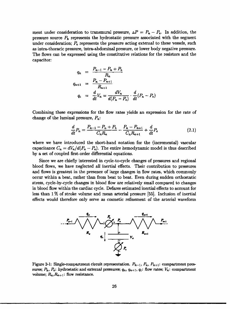
ment under consideration to transmural pressure, aP = P,- P. In addition, thepressure source Ph represents the hydrostatic pressure associated with the segmentunder consideration; Pe represents the pressure acting external to these vessels, suchas intra-thoracic pressure, intra-abdominal pressure, or lower body negative pressure.The flows can be expressed using the constitutive relations for the resistors and thecapacitor:

Pn-1 -P + Phqn = n -qni - n - Pn+1

d dV = d P e)dt d(Pn - P) dt(P

Combining these expressions for the flow rates yields an expression for the rate ofchange of the luminal pressure, Pn:

d P,-1 - P+ Ph Pn - Pn+I dP,= + Pe (2.1)dt CnR Cn~+l + dt

where we have introduced the short-hand notation for the (incremental) vascularcapacitance Cn = dVn/d(Pn - Pe). The entire hemodynamic model is thus describedby a set of coupled first-order differential equations.

Since we are chiefly interested in cycle-to-cycle changes of pressures and regionalblood flows, we have neglected all inertial effects. Their contribution to pressuresand flows is greatest in the presence of large changes in flow rates, which commonlyoccur within a beat, rather than from beat to beat. Even during sudden orthostaticstress, cycle-by-cycle changes in blood flow are relatively small compared to changesin blood flow within the cardiac cycle. Defares estimated inertial effects to account forless than 1% of stroke volume and mean arterial pressure [55]. Inclusion of inertialeffects would therefore only serve as cosmetic refinement of the arterial waveform

V.

Figure 2-1: Single-compartment circuit representation. Pn-1, Pn,, Pn+1: compartment pres-sures; Ph, Pe: hydrostatic and external pressures; qn, qn+l, qc: flow rates; Vn: compartmentvolume; Rn,Rn+l: flow resistance.

26

q. I

Figure 2-2: Circuit representation of the hemodynamic system. IVC: inferior vena cava;SVC: superior vena cava. Numbers indicate compartment index.

27

morphology and would come at an increased computational cost.The topology of the entire hemodynamic system is modeled in Figure 2-2. The

peripheral circulation is divided into upper body, renal, splanchnic, and lower bodysections on the basis that they receive similar fractions of cardiac output [56]. Thesuperior vena cava and the intra-thoracic and abdominal portions of the inferior venacava are separately identified, as are the ascending aorta, the brachiocephalic arteries,and the thoracic and abdominal portions of the aorta. The arterio-venous resistancesof the four peripheral vascular beds have not been assigned to particular arterial orvenous compartments as their properties are representative of the respective micro-circulations. The latter are described primarily by their resistive properties and areassumed to exhibit negligible capacitive characteristics. The systemic circulation thusconsists of fifteen compartments, each of which requires specification of a resistance,a pressure-volume relation, and an effective anatomical length. The latter will beused to determine the compartments' hydrostatic pressure components in the erectposture. Since we will neglect gravitational gradients in the anterior-to-posteriordirection, the effective anatomical lengths are the projections of the vessel lengthsonto the major body axis.

Since the entire peripheral vasculature is represented by only four vascular beds,it is important for our later discussion of blood volume and blood flow distributionto be clear about which anatomical structures are assigned to which vascular bed.We assume the upper body compartment to represent the circulation of the head, theneck, and the upper extremities. The latter are assumed to account for 10 % of totalskeletal muscle mass. Furthermore, we assume that one third of the blood supply tothe skin and one half of the blood supply to the skeleton occurs in the upper bodycompartment. The renal compartment represents the kidneys and the adrenal glands.The splanchnic compartment comprises the entire gastro-intestinal tract, one half ofthe adipose tissue, and one third of the skin. Finally, the leg compartment representsthe lower extremities and the pelvic circulation. As such, it contains 90 % of theskeletal muscle, one half of the skeleton, one third of the skin, one half of the adiposetissue, and the pelvic organs.

2.1.2 Parameter AssignmentsBelow and in sections to follow, we discuss in detail the rationale for the numericalvalues assigned to the various physical parameters of the hemodynamic system. Inreviewing the medical literature, we strive to characterize each parameter by givingestimates for its population mean, its standard error, and, where possible, providea reasonable physiological range. Since the choice of parameter values will definethe nominal cardiovascular state of the model, we first comment on what we intendthis nominal state to represent and which a priori assumptions this representationnecessitates.

The main focus of this work is to understand the physiological response to ortho-static stress in normal, healthy subjects, of whom we consider astronauts to constitutea subset. The cardiovascular state of the model must therefore be representative ofa normal, healthy subject population. However, it is well established that particu-

28

larly blood volume scales with the size of the subject under consideration [57]. InTable 2.1, we summarize anthropometric and cardiovascular variables for the subjectpopulation we aim to represent. The data are based on sizable clinical studies ofnormal male subjects who are assumed free of cardiovascular pathology [57-62]. Inthe following, we therefore assume a 169 cm, 70 kg subject with a total blood volumeof 5150 ml and cardiac output of 4813 ml/min.

Vascular Lengths To determine the hydrostatic pressure component to be as-signed to each compartment, we need to supply an estimate of the superior-to-inferiorextension of the vascular segments each compartment represents. For most compart-ments, such as, for example, the thoracic aorta, this estimate is identical with theiranatomical length, as their primary orientation is parallel to the major body axis.For the upper body, renal, and splanchnic compartments, however, this does nothold true and we estimate the vascular lengths of these compartments by their aver-age inferior-to-superior extension measured from the point of origin of their arterialblood supply.

Obtaining detailed measurements of vascular segment lengths from the literatureproved to be surprisingly difficult, so we had to rely on anthropometric studies [61]and standard anatomy textbooks [63, 64] to assign most nominal values.

We represent the hydrostatic contribution of the blood column in the left ventricu-lar outflow tract, the ascending aorta, and parts of the aortic arch by a single, lumpedhydrostatic pressure component. Assigning to the outflow tract half the base-to-apexlength of the heart, which is about 10 cm [65], and using Gray's estimate of 5 cm [63,p. 1504] for the length of the ascending aorta, we can assign an anatomical lengthof approximately 10 cm to the aortic root compartment. Similarly, using Gray's esti-mate of 4 to 5 cm [63, p. 1513] for the brachiocephalic artery, we can assign a nominalvalue of approximately 4.5 cm to the compartment representing the ascending tho-racic arteries. The corresponding compartment on the venous side represents partsof the right atrium, the superior vena cava, and the brachiocephalic veins. Since theycover the same vertical height as the corresponding segments on the arterial side,their hydrostatic contributions have to be equal. Assigning 7 cm [63, p. 1592] to thesuperior vena cava and 2.5 cm to the right brachiocephalic vein [63, p. 1591] leaves

Table 2.1: Population characteristics of anthropometric and cardiovascular variables. BSA:body surface area; TBV: total blood volume; CO: cardiac output; MAP: mean arterialpressure; CVP: central venous pressure.

Height Weight BSA TBV CO MAP CVPcm kg m2 ml ml/min mm Hg mm Hg

(169.3 ± 1.5) (70.3 ± 2.1) (1.83 ± 0.02) (5150 ± 124) (4813 ± 103) (91 ± 2) (6 ± 2)

(161.5-186.8) (59.8-98.5) (1.51-2.10) (3750-6890) (4344-7602) (84-103) (2.2-9.6)

Data represent mean ± standard error and (0.05 - 0.95) interquantile range.

29

the remaining 5 cm to be assigned to the right atrium, which is about one half of theheight of the heart. The remainder of the right atrium and the thoracic inferior venacava account for a height of approximately 6 cm. Finally, at the level of the diaphragmthe hydrostatic contribution in the descending aorta must be equal to the hydrostaticcontribution in the thoracic inferior vena cava, which implies the descending aorta tohave a nominal length of 16 cm.

Using ultrasonography in 180 adult healthy volunteers, Macchi and Catini [66]report the lengths of the infra-renal portions of the abdominal aorta and inferiorvena cava to be (8.31 ± 0.22) cm with a range of (5.9 - 10.5) cm and (9.52 ± 0.27) cmwith a range of (5.8 - 13.6) cm, respectively. The latter value agrees with the workby Bonnichon and co-workers [67] who used cavography to measure the length of theinfra-renal inferior vena cava in 100 subjects, and report an average length of 9.6cmwith a range of (8.0 - 14.2) cm. Martini [64] suggests that the renal arteries are locatedabout 2.5 cm distal to the superior mesenteric artery, which in turn branches off theabdominal aorta approximately 2.5 cm distal to the coeliac trunk. The combineddata therefore suggest a length of the inferior vena cava and abdominal aorta ofapproximately 14 to 15 cm.

The lower extremity compartment of our model represents the vasculature of thelegs and pelvis. Its anatomical height is approximated by the waist height, whichis the vertical distance from the floor to the top of the iliac crest and has beenmeasured in 24,469 US Army men [68] to be (105.6+5.0) cm with a range of (94.2- 117.6) cm. This estimate is justified as the aortic bifurcation occurs at the baseof the fourth lumbar vertebra which in turn is level with the iliac crest [63, p. 426].The vasculature of the neck, the head, and the arms is lumped into a single upperbody compartment to which we assigned a lumped vertical distance of 20cm. Thisvalue corresponds to the length of the common carotid arteries [63, p. 1514]. Thekidneys are approximately symmetrical in shape about the transverse plane definedby the renal arteries and veins. As such, their superior-to-inferior extension does notcontribute further to blood pooling and their effective hydrostatic length is assumed tobe zero. Lastly, the splanchnic compartment comprises the circulation of the liver, thespleen, the pancreas, and the gastrointestinal tract which anatomically span the entireabdominal cavity. We assume most of the compliance of the splanchnic circulation toreside in the small and large intestines and assume their effective hydrostatic length

Table 2.2: Anatomical lengths of arterial vascular segments. Values given in cm. Compart-ment indices are from Figure 2-2.

Compartment Index1 2 3 6 7 8 10 12

Mean 10 4.5 20 16 14.5 0 10 106Range (9-11) (4-5) (18-22) (14-18) (11-19) (0.0-0.1) (9-11) (94-118)

30

to be zero as well.In closing the discussion on the lengths of the individual vascular segments, it

should be pointed out that the data for the arterial components described above areall in good agreement with the estimates presented by Avolio [69] and Noordergraafand co-workers [70]. Since it is unclear whether their estimates are based on actualanatomic investigations, we chose to justify the parameter assignments independentlyof their work. Our estimates of the anatomic lengths of the vascular compartmentsare summarized in Tables 2.2 and 2.3 where we have assigned the upper and lowerlimits in the general population to be + 10 % of the nominal value for variables whereexperimental ranges could not be found.

Pressure-Volume Relations Blood vessels behave like distensible tubes in thatthey require a certain amount of volume (the unstressed or zero-pressure filling vol-ume) in order to be distended at zero transmural pressure; their vascular volumerises in an approximately linear fashion at low enough transmural pressures, andthey exhibit an elastic limit at high transmural pressures. Figure 2-3 illustrates thesecharacteristics for a human aorta and its major subdivisions [71]. It also demonstratesthat the compliance of the human aorta changes not only as a function of transmuralpressure but also along the length of the vessel. While the elastic properties of vascularsegments are fully specified by their (non-linear) pressure-volume relationships, underbaseline physiological conditions most vessels operate in a range of transmural pres-sures over which their pressure-volume relations can be presumed linear. Under theassumption of a linear pressure-volume relation over the range of 60 - 140 mm Hg, thedata in Figure 2-3 suggest compliances per unit vessel length of 0.008 ml/mm Hg/cm,0.017 ml/mm Hg/cm, and 0.028 ml/mm Hg/cm for the abdominal aorta, the thoracicaorta, and the ascending aorta, respectively. When analogously normalized by thelengths of the vessel segments, the unstressed volumes are 0.7ml/cm, 1.0 ml/cm,and 2.1 ml/cm. The values of 1.0ml/cm and 0.017ml/mm Hg/cm for the thoracicaorta compare very favorably with the values (1.20 ± 0.15) ml/cm and (0.013 i0.002) ml/mm Hg/cm that can be estimated from the data reported by Hallock andBenson [72] and reproduced in Figure 2-4. Assuming the same percentage errors,we assign (0.7 i 0.09) ml/cm and (0.007 ± 0.001) ml/mm Hg/cm to the abdominal

Table 2.3: Anatomical lengths of venous vascular segments. Values given in cm. Compart-ment indices are from Figure 2-2.

Compartment Index4 5 9 11 13 14 15

Mean 20 14.5 0 0 106 14.5 6Range (18-22) (13-16) (0-1) (0-2) (94-118) (11-19) (5-7)

31

t-

_80-

0.

Ern Aor .a"

i 2.5

_Ao ~u25

At 1.51.0

Abdon" IA-qsO.

- ' ' ' ' ' O.J1 6 0 1 10 200 20 60 0 Ix so 20D 25X

Tinmuural Prema Tnmwunl PRmure(rmm H) (mn Hg)

Figure 2-3: Pressure-volume relation of a Figure 2-4: Volume per unit length of tho-human aorta. Segment lengths indicated in racic aorta. Solid line: population mean;parentheses. Data adapted from [71]. dashed lines: standard deviation. Data

adapted from [72].

aorta, (1.0 ± 0.13) ml/cm and (0.013 ± 0.002) ml/mm Hg/cm to the thoracic aorta,and (2.1 ± 0.3) ml/cm and (0.028 ± 0.004) ml/mmHg/cm to the ascending aorta,respectively. Furthermore, we assume negligible difference between the histologicalstructure of the ascending aorta and the brachiocephalic arteries and assign the sameper-length values of unstressed volume and vascular compliance to that compartment.

Reliable experimental values for the lumped arterial compliances of the periph-eral vascular beds could not be obtained from the literature. In estimating thesevalues, we assume that the compliance per unit length of the leg arteries is (0.004 ±0.001) ml/mm Hg/cm, or approximately half the value of the abdominal aorta. Fur-thermore, we assign the same value, namely (0.42 ± 0.1) ml/mmHg, to the upperbody and splanchnic compartments and half that value to the renal arterial com-partment. The total compliance of the systemic arterial system thus equates to(2.19 ± 0.27) ml/mm Hg.

During orthostatic stress, the venous transmural pressures in parts of the depen-dent vasculature can reach levels at which the non-linear nature of their pressure-volume relations become important [73, 74]. This phenomenon was investigated byHenry [75], who used water-displacement plethysmography to measure changes in thevolume of both legs as a function of increments in venous distending pressure. Hisdata for one subject are reproduced in Figure 2-5. It should be recalled that the legcompartment in our model represents the dependent limbs and the pelvic circulation.Figure 2-6 shows the pressure-volume relation of a common iliac vein [76]. Under theassumption that the right and left common, internal, and external iliac veins have thesame physical characteristics, the pelvic venous vasculature accommodates roughlyone tenth of the venous volume of the legs at physiological transmural pressures,and has about 4% of their vascular compliance. A non-linear model of the venouspressure-volume relation has been implemented assuming a functional relationship

32

A_ An_MU-

1* 4nk

500-

200:

i

3.5-

.0 20-

1.S-

10

0 26 GO 75 100 -o 6 0 6 10

Venaus Pm h emnt" Trnsnwure

Figure 2-5: Pressure-volume relation of Figure 2-6: Pressure-volume relation of aboth legs. Data (filled circles) adapted from common iliac vein. Data (filled circles)[75]. adapted from [76].

between total vascular volume, Vt, and transmural pressure, AP, of the form

Vt(aP) = V0 + m arctan AP for P > P27fr p 2 0

where Vma, denotes the distending volume limit of the lower body compartment,Co is the vascular compliance at zero transmural pressure, and V0 is the venousunstressed volume. Synthesizing the information from Figures 2-5 and 2-6, we assign(1200 ± 100) ml to Vma, and (20 ± 3) ml/mm Hg to Co. The data reviewed by Leggettand Williams [77] suggest a total blood volume of the legs, pelvis, and buttocks ofapproximately 1112 ml in the supine posture if one assumes that the leg and glutealmuscles make up the majority of skeletal muscle in the human body. Accountingfor 160ml and 36 ml of distending volume for the venous and the arterial vessels,respectively, suggests an unstressed volume of 916 ml of which we assign (200 + 20) mlto the arterial compartment and the remaining (716 ± 50) ml to the venous side.

Figure 2-6 can also be used to obtain an estimate of the compliance of the inferiorvena cava which is formed by the confluence of the right and the left common iliacveins. Assuming that the physical properties of the inferior vena cava are not signif-icantly different from the ones of the common iliac veins, and combining the data inFigure 2-6 with the morphometric analyses by Macchi and Catini [66], one can esti-mate the caval compliance per unit length to be (0.09±0.01) ml/mm Hg/cm. Combin-ing this value with the length estimates from Table 2.3 yields (1.3 ± 0.1) ml/mm Hg,(0.5 ± 0.1) ml/mm Hg, and (1.3 ± 0.1) ml/mm Hg for the compliances of the abdomi-nal, the thoracic inferior, and the thoracic superior vena cava, respectively. Assuminga central venous pressure of (6 ± 2) mm Hg in combination with the compliance of(1.8 ± 0.1) ml/mm Hg for the entire inferior vena cava suggests a distending volume of(10.8 i 3.6) ml. The data by Macchi and Catini cited above suggest a total volume ofthe inferior vena cava of (116 ± 12) ml which, in turn, suggests an unstressed volumeof (53 ± 13) ml or (5.5 ± 0.6) ml/cm.

33

---

. . . . . . . .

The splanchnic circulation is the most capacious vascular bed and the principalreservoir of blood volume in the entire circulation. Under normal physiological con-ditions, it is estimated to contain about (20-26)% of total blood volume [77] andto receive about 25% of cardiac output [56]. Animal experiments in dogs suggesta specific splanchnic vascular compliance of (1.0 ± 0.4) ml/mm Hg/kg body weight[78]. While it would be fallacious to extrapolate from this value to the human bodyas the spleen of the dog in particular is a much bigger relative blood reservoir thanit is in the human [79], the specific vascular compliance of the dog does provide anupper bound on the venous vascular compliance of the human splanchnic vascularbed. Rowell [80, p. 207] cites a specific vascular compliance of 2.5 ml/mm Hg/kg oftissue weight for the intestines and suggests ten times this value for the liver. Com-bining these estimates with the dry tissue masses for humans tabulated by Leggettand Williams [77] suggests an average human splanchnic venous compliance of ap-proximately 50 ml/mm Hg. We shall assume a value of (50 ± 7.5) ml/mm Hg wherethe relatively large uncertainty is reflective of the lack of more accurate experimentsto refine the estimate. The data compiled by Leggett and Williams [77] also suggesttotal splanchnic blood volume to be 1880 ml. Assuming an arterial unstressed volumeof (300 ± 50) ml and a splanchnic venous pressure of 8 mm Hg suggests an unstressedvolume of (1142 ± 100) ml for the splanchnic venous circulation.

The kidneys are thought to contain (2.0 + 0.7) % of total blood volume or (120 40) ml [77]. Assuming arterial renal unstressed volume to be (20 ± 5) ml and account-ing for another (20 ± 5) ml of arterial stressed volume leaves approximately 80 ml ofrenal venous volume. Assuming a venous vascular compliance of (5 + 1) ml/mm Hgsuggests a venous unstressed volume of (30 + 10) ml.

Finally, the circulation of the head, the neck, and the upper limbs constitute theupper body compartment to which we assign (18.2 ± 2.9) % of total blood volume,or (937 ± 90) ml, based on the percentage estimates tabulated in [77]. The arterialdistending volume is approximately (38±8) ml. When assuming an arterial unstressedvolume of (200 ± 40) ml we are left with a total venous volume of approximately(700±50) ml. Bleeker and co-workers [81] used occlusion plethysmography to estimatethe compliance of the arm veins. Their data suggest a lumped venous compliance ofboth arms of (1.2 ± 0.2) ml/mm Hg and is probably a conservative estimate of thetrue venous compliance as their measurement of volume is made at single location.We assign a lumped venous compliance of (7 ± 2) ml/mm Hg to the upper bodycompartment which reflects our belief that the large veins in the neck contributesignificantly to the capacitance of this compartment. The venous unstressed volumeis therefore assigned the value of (643 ± 50) ml.

Resistances The largest resistance to blood flow occurs at the level of the pre-capillary arterioles within the systemic micro-circulation. We represent these resistiveproperties by a lumped resistance for each of the four micro-circulatory beds. Minorresistance to blood flow occurs along the systemic arterial and venous circulations.

Based on the data reviewed by Leggett and Williams [56] we assume 22 % (15 % -29 %) of resting cardiac output to supply the upper body compartment, 21 % (18 % -

34

Table 2.4: Parameter assignments for systemic microvascular resistances.

Microcirculationupper body kidneys splanchnic legs

R PRU (4.9 + 1.7) (5.2 ± 1.0) (3.3 ± 1.0) (4.5 ± 1.8)

24 %) to perfuse the kidneys, 33 % (24 % - 48 %) to flow through the splanchnic com-partment, and 24 % (14 % - 33 %) to represent pelvic and leg blood flow. Assuming aperfusion pressure of (87± 10) mm Hg and cardiac output of (4813 ± 103) ml/min, therespective micro-vascular resistances, where we chose to represent the numerical val-ues in terms of peripheral resistance units, PRU = mm Hg s/ml, are (4.9±1.7) PRU,(5.2 ± 1.0) PRU, (3.3 ± 1.0) PRU, and (4.5 ± 1.8) PRU for the upper body, renal,splanchnic, and leg compartments, respectively.

The resistances on the venous side can be estimated from the respective flowsand observed pressure drops along the venous system. Barratt-Boyes and Wood [60]measured the pressure drop between the inferior vena cava and the right atrium to be(0.5 ± 0.2) mm Hg, suggesting a venous flow resistance of (0.008 ± 0.003) PRU for thethoracic inferior vena cava compartment and (0.019 ± 0.007) PRU for the abdominalvena cava compartment, respectively. The authors report the same pressure dropof (0.5 ± 0.2) mm Hg between the superior vena cava and the right atrium, whichsuggests a value of (0.028 ± 0.014) PRU for the flow resistance of the superior venacava compartment. Arnoldi and Linderholm [82] report venous pressure to drop by(2.8 ± 1.1) mm Hg between various locations in the deep veins of the legs and and theright atrium. This suggests a venous resistance of (0.05 ± 0.06) PRU for the outflowresistance of the leg compartment. This resistance value is rather small and quitelikely a low estimate of the venous outflow resistance. We will assume a slightly

Table 2.5: Parameter assignments for the systemic arterial compartments. Compartmentindices are from Figure 2-2.

Compartment Index1 2 3 6 7 8 10 12

C ml 0.28 0.13 0.42 0.21 0.10 0.21 0.42 0.42mm Hg 0.04 ±0.02 ±0.10 +0.03 ±0.01 +0.05 -0.05 +0.10

V ml 21 5 200 16 10 20 300 200+3 +1 +40 ±2 +1 +5 +50 ±20

R PRU 0.007 0.003 0.014 0.011 0.010 0.10 0.07 0.09+0.002 ±0.001 +0.004 +0.003 0.003 +0:05 +0.04 +0.05

h cm 10.0 4.5 20.0 16.0 14.5 0.0 10.0 106

35

Table 2.6: Parameter assignments for the systemic venous compartments. Compartmentindices are from Figure 2-2.

Compartment Index4 5 9 11 13 14 15

C ml 7 1.3 5 50 27 1.3 0.5mmHg ±2 ±0.1 ±1 ±7.5 ±3 ±0.1 ±0.1

645 16 30 1146 716 79 33±m40 ±4 ±10 ±100 ±50 ±10 ±4

0.11 0.028 0.11 0.07 0.10 0.019 0.008RU 0.05 ±0.014 ±0.05 ±0.04 ±0.05 ±0.007 ±0.003

h cm 20.0 14.5 0.0 10.0 106 14.5 6.0

higher value of (0.10 ± 0.06) PRU for the outflow resistance of the leg compartment.Similarly, we will assume venous resistances of (0.07 ± 0.04) PRU, (0.11 ± 0.06) PRU,and (0.11±0.05) PRU for the splanchnic, the renal, and the upper body compartment,respectively.

Similarly, the pressure drop in the systemic arterial system does not exceed 2-3 mmHg between the ascending aorta and the brachial or abdominal arteries [83].Assuming a reduction in mean arterial pressure of (2 + 1) mmHg between the as-cending aorta and the abdominal aorta suggests an aortic resistance per unit lengthof (7.0 + 2.0) .10-4PRU/cm or lumped aortic resistances of (0.007 ± 0.002) PRU,(0.011 +0.003) PRU, and (0.010+-0.003) PRU for the ascending, the thoracic, and theabdominal aorta compartments, respectively. Similarly, we assign (0.003±0.001) PRUand (0.014+0.004) PRU for the arterial segments of the brachiocephalic and the upperbody compartments. Finally, we assume another pressure drop of (2 ± 1) mm Hg tooccur between the abdominal aorta and the arterial beds of the kidneys, the splanch-nic, and the leg compartments. The remaining three arterial resistances are therefore(0.10 ± 0.05) PRU, (0.07 ± 0.04) PRU, and (0.09 + 0.05) PRU, respectively. The pa-rameters of the systemic circulation are summarized in Tables 2.4, 2.5, and 2.6.

2.2 Cardiac ModelMacroscopically, cyclic changes in the heart's myocardial elastic properties accountfor its ability to pump blood from the low pressure systems (pulmonary and sys-temic veins) to the high pressure systems (systemic and pulmonary arteries). In aseries of seminal publications [84-87], Suga measured the time course of the canineinstantaneous ventricular pressure-volume ratio and demonstrated that the resultanttime-varying elastance waveforms, when properly scaled, reduce to a single, universalcurve. The analogy of a time-varying mechanical elastance (or its reciprocal, a time-varying compliance) to a time-varying electric capacitor and the fact that the scaled

36

waveform assumes a universal shape makes this description of cardiac contractionparticularly attractive, and forms the basis of the cardiac model described below.

2.2.1 Architecture

Suga's work suggests the cardiac representation shown in Figure 2-7, in which anatrial compartment is coupled to a ventricular compartment. The diodes represent therespective cardiac valves and ensure unidirectional flow. The time-varying pressuresource, Pth, represents intrathoracic pressure. To complete the description of cardiaccontraction, we have to specify the time course of the atrial and ventricular elastances,Ea(t) and EV(t), respectively.

Suga normalized the amplitudes of the canine time-varying elastance waveformsby their respective maxima, or end-systolic values, Ee, and scaled the time axis by thetime to maximal amplitude, Ts. Once scaled, the shape of the resultant normalizedwaveform turned out to be quite independent of heart rate, inotropic state, and thechamber's loading conditions (both preload and afterload) [87]. The same approachhas subsequently been used to characterize the elastic properties of the human cardiacchambers. Figure 2-8 shows recent data of the normalized time-varying elastancewaveform for human left ventricles [881 along with a functional representation thereof(blue line). The latter is described by Equation 2.2, where we represent the systolicand early diastolic portions of the elastance waveform in terms of appropriately scaledtrigonometric functions, though a representation in terms of piecewise linear segmentsis similarly justified [33, 34]. We assume the time for early diastolic relaxation, Td,to be one half of the systolic time interval Ts. This assumption seems well justifiedby the data presented.

E + es-Ed {1 - cos(7r )} O < t < TE(t) es 2E, T.

es E + EEd {1 + cos(2r t-) T < t < T, (2.2)Ee Ees 2E s T 2

Ees 2

R.,

)

Figure 2-7: Circuit model of atrial and ventricular compartments. Pa and P,: atrial andventricular pressures; Pth: intrathoracic pressure; Ca(t) and CV(t): atrial and ventricularcapacitances; Ea(t) and Ev(t): atrial and ventricular elastances. Ra-v: atrio-ventricularflow resistance.

37

----

iI

0.0 0.5 1.0 1.5 2.0 2.5 3.0

Time(normaNzed units)

Figure 2-8: Normalized time-varying elastance of the human left ventricle. Ts: systolic timeinterval; Td: time interval of diastolic relaxation. Data adapted from [88].

We assumed the shape of the normalized time-varying elastance waveforms to beidentical for all four cardiac chambers. The assignment of the respective parametersfor each chamber is discussed in detail in the following section.

2.2.2 Parameter AssignmentsThe time-varying elastance model described above requires that end-systolic elas-tance, Ees, and diastolic elastance, Ed, be assigned for each cardiac chamber, alongwith rules that specify the fraction of the cardiac cycle spent in atrial and ventricularsystole. As indicated in Figure 2-9, the determination of the end-systolic elastance ne-cessitates simultaneous beat-by-beat measurements of chamber pressures and volumesunder various loading conditions, and subsequent regression analysis of the resultingdiastolic and end-systolic pressure-volume relations. While pressure measurementscan be made routinely with high fidelity, the methods currently in use for assessingchamber volumes throughout the cardiac cycle are frequently based on simplifyinggeometric assumptions and continue to be a source of significant uncertainties.

The most extensively studied chamber is the left ventricle. Using a conductancecatheter approach for volume determination and transient inferior vena caval balloonobstruction to alter preload, Senzaki and co-workers [88] reported left ventricularend-systolic elastance in fifteen subjects to be E, = (2.0 ± 0.7) mmHg/ml. As-suming a mean body surface area of 1.9m2 , Senzaki's results seem congruent withearlier estimates by McKay [89] (ElV = (2.5 ± 0.6) mmHg/ml) and Grossman [90](El = (2.8 ± 0.8) mm Hg/ml) who used gated blood pool radionuclide ventriculog-raphy and biplane contrast cineangiography, respectively, to determine ventricularvolume, and who chose to reference their respective results to the body size of theirpatient populations. In contrast, using biplane contrast cineangiography Starling [91]

38

: l-E '-2 E25-

00-3 .

P

tiV ~ ~ ~~~~~=Ed ~~~~~

50 X10 Ie 20 250

Left Ventkuhmr Volum Enddislok Vokume(ml) (ms)

Figure 2-9: Simulated left ventricular Figure 2-10: Left ventricular end-diastolicpressure-volume loops. E: end-systolic pressure-volume relation. PCW pressure:elastance; Ed: diastolic elastance; V: un- pulmonary capillary wedge pressure. Datastressed volume. adopted from Perhonen et al. [43]

reported a significantly higher value (Elv = (5.5 i 1.2) mm Hg/ml) in ten subjects.We chose to adopt McKay's results for E.

Although the diastolic elastic properties of the ventricles are fairly linear overthe range of normal filling pressures, they do exhibit a marked non-linearity whenfilled to capacity, as illustrated in Figure 2-10. Since filling pressures decrease withincreasing gravitational stress, it is admissible to represent the diastolic pressure-volume relations of the various cardiac chambers by linear relations as indicated by thedashed line in the same figure. Information provided by Senzaki [88] and Starling [91]allows for computation of left ventricular diastolic elastance values of Ed'v (0.13 ±0.05) mm Hg/ml and Edv t (0.10 ± 0.06) mm Hg/ml, respectively. Similarly, the datapresented by Perhonen and co-workers [43] suggest E V : (0.13 + 0.02) mmHg/ml.We chose to adopt this latter value for our simulations.

The right ventricle has been studied less extensively, mostly because of its morecomplex geometry. Using biplanar contrast cineangiography, Dell'Italia and co-workers[92] report right ventricular end-systolic elastance to be Ee = (1.3 ± 0.8) mmHg/ml with a range of (0.62 - 2.87) mm Hg/ml. Using their estimate of right ven-tricular unstressed volume (VoV = (46 ± 21) ml) and their reported values for end-diastolic pressures and volumes, the diastolic right ventricular elastance equates toEd (0.07 ± 0.03) mm Hg/ml with a range of (0.02 - 0.09) mm Hg/ml.

Even less quantitative information is available for the atria. Dernellis and co-workers [93] performed echocardiographic and hemodynamic studies on the humanleft atrium. They report an end-systolic elastance of El' = (0.61 + 0.07) mm Hg/ml,a diastolic elastance of Eda = (0.50 ± 0.10) mm Hg/ml, and a left atrial unstressed vol-ume of Vo = (3.15 ± 0.42) ml. While a relatively small ratio of end-systolic to diastolicelastance has been a consistent finding in canine experiments [94], the ratio suggestedby Dernellis' data is quite low. Furthermore, it seems that the value he derived for theunstressed volume is particularly low as well. In the absence of further experiments

39

· _s._v

Table 2.7: Cardiac Model Parameters.

Right HeartAtrium Ventricle

Left HeartAtrium Ventricle

Ees mriHg (0.74-0.1) (1.3±0.8) (0.61±0.07) (2.5±0.6)

Ed Im_ (0.30±0.05) (0.07±0.03) (0.50±0.10) (0.13±0.02)

V0 ml (14±1) (46±21) (24±13) (55±10)

Ra-v PRU (0.005 ± 0.001) (0.010 ± 0.001)

on humans, one is forced to direct one's attention to detailed animal experiments.Mindful of the difficulties involved and the uncertainties introduced by such an ap-proach, one can derive scaling factors that extrapolate results obtained in differentanimal models to human physiology. If one compares the right ventricular data pre-sented by Dell'Italia in humans with the ones presented by Schwiep and colleagues[95] for mongrel dogs, one can introduce a scaling factor of 3.5 that relates the respec-tive end-systolic and end-diastolic volumes. When scaled by this factor, Schwiep'scanine end-systolic ventricular elastance translates to 1.2 mm Hg/ml which comparesfavorably with Dell'Italia's Ed' (1.3 ± 0.8) mm Hg/ml. Applying the same scal-ing factor to the left atrial data presented by Alexander [94] yields an end-systolicelastance of (0.52±0.11) mm Hg/ml, a diastolic elastance of 0.4mm Hg/ml, and anunstressed volume of (24±13) ml. The elastance values so derived are in approximateagreement with the results reported by Dernellis. The extrapolated unstressed vol-ume seems more appropriate for a human and will therefore be used in our model.When the same scaling factor is applied to the right atrial data reported by Lau andcolleagues [96] one derives an end-systolic elastance of Er = (0.74 ± 0.1) mm Hg/ml,a diastolic elastance of Eda = (0.30 ± 0.05) mm Hg/ml, and an unstressed volume ofVora = (14 ± 1) ml.

Barratt-Boyes and Wood [60] used right-heart catheter withdrawal maneuvers toinvestigate the pressure drop across the tricuspid valve during right ventricular fill-ing. The investigators found no significant difference between maximal atrial systolicpressure (atrial a-wave) and right ventricular end-diastolic pressure. There was alsono statistically significant difference between minimal right atrial pressure and initialdiastolic right ventricular pressure. We attribute these findings to a very small tricus-pid flow resistance and assign the value of (0.005±0.001) PRU to the atrio-ventricularresistance of the right heart. The data presented by Firstenberg and colleagues [97]suggest an average trans-mitral pressure gradient during diastole of approximately1 mm Hg. Combining this estimate with their data of heart rate and cardiac output,we can estimate the mitral flow resistance to be (0.010 ± 0.001) PRU. The physicalparameters of the cardiac model are summarized in Table 2.7.

To finalize the time-varying elastance description of the cardiac cycle, we needto specify the delay between the onsets of atrial and ventricular contraction, Ta-v.

40

L L

Table 2.8: Mean values and ranges of cardiac timing parameters K.

mean s 0.25 0.37 0.19

mean s 0.25 0.37 0.19

range s 0.2 - 0.3 0.34 - 0.39 0.18 - 0.20

Furthermore, we need to assign rules that specify the duration of atrial, Tsa, and ven-tricular, T, systole relative to the length of the cardiac cycle. In a strict sense, thistiming information can only be derived from the relative timing of mechanical eventsvisualized in the pressure-volume loop, such as the onsets of isovolumic contractionor relaxation. Unfortunately, these mechanical events do not correspond to precise orreadily identifiable points on conventionally recorded signals, such as pressure trac-ings or the electrocardiogram (ECG). However, if one neglects differences in relativetiming between electrophysiological and mechanical events due to the mechanisms ofexcitation-contraction coupling, one can approximate the desired timing informationwith the help of the surface ECG.

The delay between the onsets of atrial and ventricular contraction can be readilyapproximated by the P-R-interval, the time interval between the onsets of atrial andventricular depolarization. At resting heart rates the P-R-interval is normally on theorder of 180 - 200 ms. The ventricular systolic time interval can be approximatedby the Q-T-interval, the interval between the onset of ventricular depolarization andthe end of ventricular repolarization. In 1920, Bazett [98] reported an empiricalformula for the Q-T-interval that today bears his name. He established that theQ-T-interval scales with R-R-interval length, TRR, according to K. V/ where theconstant K ranges from (342 - 392) ms. Atrial repolarization occurs during ventriculardepolarization and is therefore masked by the QRS complex in the surface ECG. Theatrial systolic time interval can, however, be approximated by a value slightly largerthan the P-R-interval. We will assume that the P-R-interval and the atrial systolictime interval also scale with the square root of the R-R-interval. Finally, we assign avalue (895i125) ms and the range of (667-1300) ms to the R-R-interval [62]. Table2.8 summarizes the timing information.

2.2.3 Limitations

The cardiac contraction model described so far is based on several simplifying assump-tions that should not go unmentioned. We have already alluded to the non-linearityof the diastolic pressure-volume relation and justified its linearization for the scope ofthis work. Similarly, at very high transmural pressures the end-systolic pressure vol-ume relation will also begin to show a significant deviation from its assumed linearity.Again, the simulation of pathologically high pressures is beyond the scope of the workpresented here. However, two assumptions do pertain to our work. First, as suggestedby Figure 2-9, we assume unstressed volume to be static throughout the cardiac cy-

41

2.0

1.5

I

0.5

2.0-

,.5-

O.S

0-0.

o.50 o5s 'o.o O , . 1. 5 US bo ' 025 O.50 0.75 1.0 1.25

Thm Tho(o) ()

Figure 2-11: Left ventricular, Elv (blue) , Figure 2-12: Right ventricular, Elv (blue),and left atrial, Ela (red), elastances. and right atrial, Ela (red), elastances.

cle, that is, the volume intercept as determined by the end-systolic pressure-volumerelation is the same as the one derived from the diastolic pressure-volume relation.Animal experiments have shown consistently that the unstressed volume at the endof systole is 25% - 40% lower than the diastolic unstressed volume [94, 96] indicatinga small but potentially significant contribution to stroke volume. We can account forthis effect quantitatively by slightly decreasing the diastolic elastances of the variouschambers so that end-diastolic volumes, and thus stroke volumes, are slightly higherfor given end-diastolic pressures. Second, the time-varying elastance model describedso far assumes that the progression from the diastolic pressure-volume relation to theend-systolic pressure-volume relation is independent of the details of the interveningejection phase and of the chamber's loading conditions. Sagawa [99] reviews exper-imental evidence against this assumption and proposes modifications to the simpletime-varying elastance model. The modified "elastance-resistance" model mostly af-fects the detailed shape of the time-varying elastance and is therefore of importancefor correct reproduction of the cardiac and arterial pressure waveform morphologies[100]. Given the relative insensitivity of the end-systolic pressure-volume relation 1

[99], we assume this modification to be of higher (and therefore negligible) order fordetermination of beat-to-beat stroke volume which is most crucial to our analysishere.

As previously mentioned, simultaneous measurements of cardiac pressures andvolumes are needed to determine cardiac elastance parameters. In concluding thissection, it is worthwhile to comment on the experimental difficulty involved and pos-sible bias introduced in conducting such studies in humans. Advances in cathetertechnology enabled cardiac chamber pressures to be measured with a remarkable de-gree of accuracy. The highly invasive nature of these measurements, however, usuallyallows for their employment in the left heart only when medically necessary. Havingto restrict the study population to those patients in whom cardiac catheterization

'It is important to point out that the ventricular end-systolic pressure-volume relations changesignificantly under inotropic stimulation. Reflex control is the topic of the next chapter.

42

^r

_ ---

is medically indicated introduces significant selection bias, not least in terms of ageand gender, such that the results derived are not necessarily reflective of the pop-ulation at large. The same holds true for volume measurements that are based oncatheterization, such as cineangiography or conductance catheter approaches, or theadministration of radionuclides, such as radioisotope imaging. In contrast to pressuremeasurements, volumetric assessment of the various cardiac chambers can at bestbe described as approximate. Several techniques currently in use, such as cinean-giography and biplanar echocardiography, rely on simplifying geometric assumptionsthat might hold true to some degree for the left ventricle. The other cardiac cham-bers have significantly more complex geometries which render simple approximationsmore questionable. Most methods to determine cardiac chamber volumes have beendemonstrated to correlate favorably with each other. In the absence of an overallgold standard, however, these correlations do not reveal systematic errors that arebound to be present. Magnetic resonance imaging (MRI) and, more recently, four-dimensional (space and time) phased-array ultrasound imaging are modalities freeof geometric assumptions having the potential of becoming the much-needed goldstandards. At this point, however, volume measurement by MRI is still limited byrelatively long acquisition times (~ 10 minutes for one average cardiac cycle) and 4-dultrasound imaging is an emerging technology that still seems in its validation phase[101].

2.3 Pulmonary CirculationThe pulmonary circulation is characterized by low resistance and high compliance inorder to accommodate, at low pressures, the same flow per unit time as the entiresystemic circulation. Local pulmonary blood flow and volume are therefore exquisitelysensitive to even small variations in perfusion or transmural pressures that naturallyoccur with changes in hydrostatic pressure components. The pulmonary capillaryvasculature, in particular, can exhibit interesting nonlinear flow phenomena, such asflow limitation and complete cessation of flow during vascular collapse, as a result ofchanges in luminal or extra-luminal pressures.

Below, we describe the architecture and parameter assignments for the pulmonaryvascular model with specific emphasis on representing a gravity-dependent nonlinearpulmonary pressure-flow relation.

As indicated in Figure 2-13, we represent the pulmonary circulation by passivepulmonary arterial and venous capacitances, Cpa and Cpv, and a nonlinear pulmonarymicrovascular resistance, Rp. Central to the model of the flow-dependent resistanceto be developed below is the understanding of the behavior of a Starling resistor [102]shown in Figure 2-14, modeling the flow-characteristics of a pulmonary capillary. Theexperimental set-up involves a pressurizable chamber with rigid inlets and outletsbetween which a thin-walled, collapsible tube is fastened. Brower and Noordergraaf[103] noted that the steady-state behavior of the Starling resistor can be described byone dependent and two independent variables. The former is usually taken to be the

43

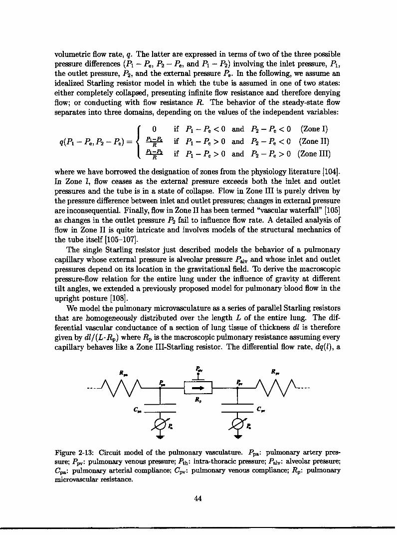
volumetric flow rate, q. The latter are expressed in terms of two of the three possiblepressure differences (P1 - Pe, P2 - Pe, and P1 - P2) involving the inlet pressure, P1,the outlet pressure, P2 , and the external pressure Pe. In the following, we assume anidealized Starling resistor model in which the tube is assumed in one of two states:either completely collapsed, presenting infinite flow resistance and therefore denyingflow; or conducting with flow resistance R. The behavior of the steady-state flowseparates into three domains, depending on the values of the independent variables:

0 if P - Pe < 0 and P2 -Pe < 0 (Zone I)

q(P - Pe, P2 - Pe) = " if P - Pe > 0 and P2 - Pe < 0 (Zone II)

P1 2 if P - Pe > 0 and P2-Pe > 0 (Zone III)

where we have borrowed the designation of zones from the physiology literature [104].In Zone I, flow ceases as the external pressure exceeds both the inlet and outletpressures and the tube is in a state of collapse. Flow in Zone III is purely driven bythe pressure difference between inlet and outlet pressures; changes in external pressureare inconsequential. Finally, flow in Zone II has been termed "vascular waterfall" [105]as changes in the outlet pressure P2 fail to influence flow rate. A detailed analysis offlow in Zone II is quite intricate and involves models of the structural mechanics ofthe tube itself [105-107].

The single Starling resistor just described models the behavior of a pulmonarycapillary whose external pressure is alveolar pressure Pv and whose inlet and outletpressures depend on its location in the gravitational field. To derive the macroscopicpressure-flow relation for the entire lung under the influence of gravity at differenttilt angles, we extended a previously proposed model for pulmonary blood flow in theupright posture [108].

We model the pulmonary microvasculature as a series of parallel Starling resistorsthat are homogeneously distributed over the length L of the entire lung. The dif-ferential vascular conductance of a section of lung tissue of thickness dl is thereforegiven by dl/(L.Rp) where Rp is the macroscopic pulmonary resistance assuming everycapillary behaves like a Zone III-Starling resistor. The differential flow rate, dq(l), a

Figure 2-13: Circuit model of the pulmonary vasculature. Ppa: pulmonary artery pres-sure; Ppv: pulmonary venous pressure; Pth: intra-thoracic pressure; Pa,: alveolar pressure;Cpa: pulmonary arterial compliance; Cpv: pulmonary venous compliance; Rp: pulmonarymicrovascular resistance.

44

---

Preurized Chamber

,/ / // /// ///////IC

.. ,,,,,,

Figure 2-14: Starling resistor. P: inletpressure; P2: outlet pressure; Pe: externalpressure; q: flow rate. Figure adapted from[107].

Figure 2-15: Schematic lateral view of thelung. L: apex-to-base length of the lung;1: distance from left atrium; dl: differentiallength element; a: tilt angle.

distance from the level of the main pulmonary artery and vein, is given by:

0

Ppa-pgl sin(a)-P1,av dLRp

Pp'-Pp dlLRp

if Ppa - pgl sin(a) - P < 0and Ppv - pgl sin(a) - Pav < 0

if Ppa - pgl sin(a) - Palv > 0and Ppv - pgl sin(a) - Pa < 0

if Ppa - pgl sin(a) - Paiv > 0and Ppv - pgl sin(a) - Pal > 0

Lewis and Christianson [109] estimated the basal-to-apical length of the lung in fifteensubjects and determined a mean value of L = 23.6 cm with 19.3 cm residing above thelevel of the left atrium (see Figure 2-15). Assuming, therefore, that 20 % of the lungparenchyma is located below the level of the main pulmonary artery and vein, wecan integrate the differential flow to obtain the macroscopic pulmonary pressure-flowrelation:

= 4L = P -Pvdl |2 PPa- pglsin(a) - Palv dlf 8_·dq=l) f Pp v: LRp LR5 ~~5

_ Ppa - Ppv- _ _ _ _ _ _ _ _ _ ( 1 LRP

+ Ppa) + -Pav sin(a) (12 -12)11 and 12 specify the boundaries between Zones II and III and Zones I and II, respec-tively, and are implicitly defined through:

pgll sin(a) = Ppv - Pv and pgl2 sin(a) = Ppa - Pajv,

subject to the constraint -L/5 < 11, 12 < 4L/5. To determine the nominal value of

45

dq(l) =

the macroscopic pulmonary vascular resistance Rp, we pooled data from four studies[110-113] to arrive at a reasonable sample size (27 subjects) for control subjectswithout cardiovascular or pulmonary pathologies. The resultant value is (0.07 ±0.04) mm Hg s/ml with a range of (0.01-0.16) mm Hg s/ml. Since we currently donot model respiratory variation in intra-thoracic or alveolar pressure, we assume meanalveolar pressure to equal atmospheric pressure [114, p. 433].

To finalize the description of the pulmonary model, we have to supply nominal val-ues for the pulmonary arterial and venous compliances and unstressed volumes. Usinga Windkessel model to represent the pulmonary arterial compartment, Reuben [113]and Milnor and co-workers [112] have estimated the lumped pulmonary arterial com-pliance from the diastolic decay of pulmonary arterial waveforms. When one's atten-tion is restricted to the pulmonary normotensive group in Reuben's study population,his data suggest a pulmonary arterial compliance of (3.0 ± 0.6) ml/mm Hg. Milnor'sestimate of (3.4 ± 1.8) ml/mm Hg is based on a group of eight patients with normalpulmonary vascular resistance but elevated mean pulmonary artery pressures. Thesetwo estimates are compatible with the widely-used value of 4.3 ml/mm Hg quotedby Beneken and DeWitt [115, p. 19] but certainly too low if one were to believeGuyton [114, p. 445] who suggests a pulmonary arterial capacitance of 7 ml/mm Hg.Guyton's suggestion that the latter value is similar to the compliance of the entiresystemic arterial tree seems a gross overestimation based on the data presented inSection 2.1.

The determination of pulmonary venous compliance in vivo is quite difficult andusually laden with assumptions that render experimental results rough estimates ofthe truth. In two publications, Hirakawa [116, 117] developed an empirical formula torelate the rise in pulmonary capillary wedge pressure during ventricular systole to achange in the combined pulmonary venous and left atrial volume. His estimates fromtwo studies, when scaled to a 75-kg male subject, equate to (9.8 ± 4.0) ml/mm Hg[117] and (9.0 ± 3.7) ml/mm Hg [118]. When accounting for the diastolic complianceof the left atrium, these values are compatible with 8.5 ml/mm Hg quoted by Benekenand DeWitt [115] for the pulmonary venous compliance.

Historically, estimates of pulmonary blood volume have ranged from 9% [114,p. 445] to over 20 % [119] of total blood volume. Leggett and Williams [77] reviewed23 studies of pulmonary blood volume and suggest a reference value of (12.5 ± 2.5) %.Burton [120, p. 64] determined, in a single subject, pulmonary arterial blood volumeto account for 30 % of total pulmonary blood volume. This value agrees with datatabulated by Milnor [121]. With these numbers and assuming a mean pulmonaryartery pressure of 16mm Hg, we can estimate the zero pressure filling volume ofthe pulmonary artery to be approximately (160 ± 20) ml for a 75-kg male subject.Analogously, the venous zero pressure filling volume equates to (430±50) ml, assuminga mean pulmonary venous pressure of 9 mm Hg.

Barratt-Boyes and Wood [60] measured the pressure gradient across the pulmonicvalve during catheter withdrawal in 21 healthy subjects to be (2.0 ± 0.3) mm Hg. Onecan arrive at an upper bound for the inflow resistance, Rpa, to the pulmonary arterialcompartment by assuming that the entire stroke volume is ejected over the systolic

46

Table 2.9: Nominal parameter values for the pulmonary circulation.

PulmonaryArteries Veins

C ml (3.4 + 1.8) (9.0 + 3.7)mm Hg

V0 ml (160 ± 20) (430 ± 50)

R PRU (0.006 ± 0.003) (0.006 ± 0.003)

time interval T, which leads to a value of Rpa < (0.006 ± 0.003) PRU. This value isan upper estimate since the ejection period is smaller than the systolic time interval.Similar data is not available for the pulmonary venous outflow resistance, Rpv. Wewill simply assume a similarly low value.

Finally, we adopt Daly and Bondurant's estimate of (-3.0±0.5) mm Hg for intra-thoracic pressure [122].

2.4 Orthostatic Stress SimulationsThe transition from the supine to the upright posture constitutes a significant chal-lenge to the cardiovascular system, as gravity induces a primary, rapid intravascularfluid shift from the thoracic to the dependent vasculature and a consequent secondary,slow fluid shift from the intravascular to the interstitial fluid compartment. Both fluidshifts act in concert to provoke a state of central hypovolemia that elicits a sequenceof reflex responses to counteract a reduction in arterial pressure and central bloodvolume. Artificial orthostatic stress tests such as lower body negative pressure inter-ventions or short radius centrifugation are designed to induce similar perturbationsin cardiovascular homeostasis.

In the following sections, we introduce three commonly used orthostatic stresstests and outline how the primary and secondary fluid shifts have been representedfor each.

2.4.1 Tilt Table SimulationTolerance to gravitational stress is commonly assessed clinically by passively tiltingsubjects to the head-up position while heart rate and arterial blood pressure are beingmonitored. As opposed to standing up, passive tilts aim to minimize hemodynamiceffects associated with muscle contraction of the lower extremities and the abdominalwall. As described in the remainder of this section, the effects of tilting will berepresented by changes in hydrostatic pressure components, changes in intra-thoracicpressure, and changes in total blood volume.

During the transition to the head-up posture, the major vascular segments gradu-ally become aligned with the direction of the gravitational field and, therefore, hydro-

47

45

40-

35-

* 30-

> 25-8 20-

F 15-

10-

5-n

at Tfi at

, q

Or___________- -

0 2 i 4 6 8 10 184 188 188 190 192 194

to Time(s)

Figure 2-16: Tilt angle a(t) during a rapid tilt to (left) and from (right) 300 head-up. to:time of tilt onset; At: tilt time; Ttilt: time in head-up position.

static pressure components become significant determinants of blood flow and bloodvolume distribution. As alluded to in Section 2.1, each vascular segment modeled hasthe provision for specifying a hydrostatic pressure component, Ph, which is given by

Ph = pgh sin (a(t)) (2.3)

where p is the density of blood, and, in the context of gravitational stress on earth, g isearth's gravitational acceleration; h is the effective length of the vascular compartmentunder consideration and the angle a(t) represents the orientation of the particularvessel segment with respect to the horizontal plane. It is the changes in Ph thatare responsible for the rapid intravascular volume redistribution at the beginning ofgravitational stress.

For a passive head-up tilt to a maximal angle am over a time interval of lengthAt, we assume the time course of a(t) to be

0 for t < toa(t) = am - (1-cos (rt-tf)) for to < t < to + at (2.4)d r at// -2-

almax for t > to + at

where it is implicitly assumed that all vessels are aligned in the horizontal plane inthe supine position and that the change in posture is initiated at some arbitrary timepoint to. The transition from the head-up to the supine posture can be modeled inanalogy to the approach outlined above as illustrated in Figure 2-16. We termed hthe effective length of the vascular compartment under consideration to distinguishit from the anatomical length of the vascular segments each compartment represents.The latter have been discussed in Section 2.1 and tabulated in Tables 2.2 and 2.3.

48

1C

The distinction is important as each compartment is a lumped representation of theaggregate function of various anatomical structures, and in order to simulate represen-tative pressures, volumes and flows, h has to represent the effective hydrostatic heightof each lumped compartment. We assume h to be one half of the superior-to-inferiorextension of the anatomical structures comprised in each compartment.

In addition to changes in the luminal pressures described by Ph, Mead and Gaensler[123] and Ferris and co-workers [124] showed that intra-thoracic pressure, Pth, changedover similarly short periods of time in response to gravitational stress. Mead andGaensler reported intra-thoracic pressure to drop by (3.1±1.0) mm Hg in response tositting up from the supine position. Ferris demonstrated a drop of (3.5±0.7) mm Hgin response to head-up tilts to 90°. We implemented these changes in intra-thoracicpressure by assuming a time course similar to the one described by Equation 2.4.

Changes in the hydrostatic pressure components in the circulation affect the bal-ance between hydrostatic and oncotic pressure gradients across capillary walls thatgovern transcapillary fluid exchange. During orthostatic stress, transcapillary hy-drostatic pressure gradients change, depending on the nature of the stress and thelocation of the capillary bed. However, the net effect of orthostatic stress is an in-crease in transcapillary fluid flow and a resultant decrease in intravascular volume.Several studies have been devoted to identifying the magnitude and the time course ofplasma volume reduction upon assumption of the upright posture, or plasma volumerestitution upon resumption of the supine position (see, e.g., [125] and the referencestherein). While Tarazi and co-workers [126] report a modest decline in plasma volumeof only (4.1 ± 0.8) % over a 20-minute period of 50° head-up tilt, Hinghofer-Szalkayand Moser [127] report plasma volume to drop by as much as 16.8 % in response toa 70° head-up tilt. This difference cannot be explained solely on the basis of thedifference in gravitational stress. During quiet standing, the data presented by Ja-cob et al. [36] suggest a reduction in plasma volume by 12.8 % whereas Hagan andco-workers [128] demonstrate a reduction by 16.2 %. A similar discrepancy emergeswhen looking at the time constants of plasma volume reduction. Tarazi's data suggesta time constant of (12.2 ± 0.3) min whereas Hagan reports a time constant of 7.8 min.The data presented by Jacob suggest much faster dynamics with a time constant of4.0 min. Despite these substantial differences in the rate and magnitude of volumereduction, it is a consistent finding that the data within each study are described wellby mono-exponential models. While some of the discrepancies described above mightbe attributable to the relatively small number of subjects (n < 10) enrolled in eachstudy, Lundvall and Bjerkhoel [129] have identified the location of blood sampling asa major source of systematic error. In a series of publications, these authors presenteda careful analysis of the effects of venous and arterial sampling in the upright pos-ture and devised a novel method to estimate more accurately plasma volume changesduring standing [125, 129-132]. The authors report a substantial degree of plasmavolume reduction, (17.7 ± 0.8) % or (707 + 41) ml, over a relatively short period oftime, T = (4.6 ± 0.4) min, in response to an 85° head-up tilt [125] as shown in Figure2-17. In a subsequent publication from the same laboratory, the authors comparecommonly used indices of plasma volume changes and surmise that their own previ-

49

0-

-6-

t"- 10-A-Is-

!

II

-20 .o 10 20 30 40

Thw Th20(Ire) (mh)

Figure 2-17: Percent change in plasma vol- Figure 2-18: Absolute change in plasma vol-ume during 850 HUT. Data adapted from ume upon return to supine posture. Data[125]; solid line represents best-fit exponen- adapted from [132]; solid line representstial model. best-fit exponential model.

ously reported results might have been subject to systematic underestimation of thetrue changes in plasma volume [133]. Their claim that prolonged ( 15 min) standingcan lead to a reduction in plasma volume of as much as 25 % is a conjecture theyhave yet to prove. For lack of population averaged data of plasma volume restitutionupon resumption of the supine position, Figure 2-18 shows the restitution dynamicsin one subject as reported by the same group of investigators.

The literature reviewed above indicates that the reduction in plasma volume issignificant even over short periods of orthostatic stress and has to be taken intoaccount when modeling cardiovascular adaptation to gravitational challenge. Themono-exponential nature of plasma volume reduction and restitution suggests a phe-nomenological description of transcapillary fluid flow in terms of a single RC com-partment, as shown in Figure 2-19. While one could easily incorporate an interstitialfluid space into the mathematical description of the hemodynamic model, such an ap-proach would add two parameters per compartment and would unnecessarily increasecomputational complexity. The approach taken here is to obtain analytical solutionsfor the transcapillary flow and the interstitial volume, assuming the model in Figure2-19 and a simplified hydrostatic pressure profile, such as the one shown in Figure2-20. Once known, one can subtract transcapillary flow from venous return at des-ignated, dependent circulatory compartments, which basically amounts to reducingoverall blood volume as a function of time during gravitational stress. Conversely,once gravitational stress is released, transcapillary flow reverses direction and can beadded to venous return to account for plasma and blood volume restitution.

Below, we give the analytical solutions for the transcapillary flow q and the in-terstitial fluid volume V = PC for the four regions indicated in Figure 2-20. Thesolutions depend on two parameters, the time constant r = RC and the maximalvolume Vmax = PhC. The numerical values of both depend on the nature of the stressto be modeled.

50

q 40-I 15- 3 I \ . -

R C M

Figure 2-19: RC model of interstitial com- Figure 2-20: Simplified hydrostatic pres-partment. sure profile. See text for details.

Region I: Gradual increase in orthostatic stress a over period of length at.

q(t) =Vmax (I-e-)

V(t) = Vmax ( - T(1-e ))

Region II: Full orthostatic stress during period of duration Ttilt.

q(t) = Vma. 1-e- ) .eAt

V(t) = Vmx (1- t(l-e )e - )

Region III: Gradual decline in orthostatic stress over a period of length at.

Vmax (1A(1 - e _t) t _t - (At+Ttit) Vmaxq(t) = t * + -r)e r )At at

V(t) = m (1 +) Vmi t (1 e)NNNNNN N+V(t) = Vmax'(1 a- Ttilt)) ax (t

Vmax (1 + (1 "-e- t)e-) 1i _t- t+Ttilt)At

Region IV: Post-orthostatic stress recovery of unspecified length.

q(t)- V_ m _ at) \( _ Ttilt+t t-(2t+Ttilt)V(t) = Vma. t 1-e ) * l 1-e . )- e

51

0

a -2W-

*000*

u-

E -1'0-Im-

. 10 -300:

- . -. . , -3m.

ad=UoaA.40aM 201A. 2

0 10 20 io ° 0 0 100 i 20 250 603

ThM Thn(mh) (s)

Figure 2-21: Absolute changes in plasma Figure 2-22: Absolute change in plasma vol-volume during simulated tilts. ume during three minutes of simulated tilts.

The model outlined above specifies the net intra-vascular volume loss and the nettrans-capillary leakage current as functions of time. To allow for spatially distributedleakage to occur, we assign fractions of the total volume loss and leakage currentaccording to the distribution of hydrostatic pressure heads in the various dependentvascular compartments. The volume loss and leakage current assigned to the splanch-nic compartment, for example, is given by:

VP(t) = (t) and t = p - q(t)

n n

where the summations extend over all dependent vascular compartments. Havingthus established the form of the analytical solutions, we have to supply empiricalvalues for the time constant r and the maximal interstitial volume change Vm,, forthe various gravitational stresses we intend to model.

For tilt and stand tests, we will assign these parameters according to the datareported by Lundvall [125] as discussed in the previous section. To allow for tilts todifferent angles a, we hypothesize that the maximal plasma volume loss is a linearfunction of the magnitude of the gravitational stress and therefore scales accordingto:

sin(amx)Vma,, = (700 ± 41) ml sin(85m)

The nominal value for the time constant is r = (4.6 ± 0.4) min and is assumedindependent of the tilt angle. Furthermore, as suggested by Figures 2-17 and 2-18,we assume plasma volume loss and restitution to have the same temporal dynamics.Figure 2-21 shows simulated changes in plasma volume to various angles of tilt. Figure2-22 shows the time course of simulated plasma volume loss and restitution as afunction of the transition time at.

52

.Jno. _ . . . .....

-4WIn-Y.--

- 10--5- Y.V-10--15-- : ._-'1 - , t-.s- '11

SUPINE -4X EA.i,

-5- :-5-

-15-; . .

. I.n

. ..

=1.i

... ..A.

|A

' :_ .......... _ .,...

.*---- ' . .. ..... i.........l.......... .. .... 5.v uV V. v '. ._..4 .I _ I--. 0-12 o8 4 8 12120ae24 3..... ~~~~~~~~~~~~Time

Figure 2-23: Pleural pressure, PP, and Figure 2-24: External pressures to the tho-esophageal pressure, EP, during changes in racic, abdominal, and leg vasculature duringposture. Figure taken from [123]. standing up.

2.4.2 Stand Tests

In a second, commonly used test to assess gravitational tolerance, subjects are askedto stand up actively from the lying position, and, once upright, maintain the posturewith minimal muscular contraction while heart rate and blood pressure are beingmonitored. During the transition to the head-up posture, significant abdominal andleg muscular activity occurs which affects hemodynamics by influencing the extra-luminal pressures of the abdominal and leg vasculature.

The venous circulation of the legs is richly endowed with valves which preventblood flow from reversing direction in the upright position and thus ensure venousreturn from the dependent extremities. When calf and thigh muscles are contracted,they exert significant external pressure on leg veins which tend to collapse these vesselsand propel their blood contents toward the heart - a phenomenon termed musclepumping. Arnoldi [134] showed that the venous pressure in the Vena tibialis posteriorincreases transiently by (53 - 158) mm Hg with a mean of 75 mm Hg in response to asingle forceful contraction of the flexor muscles of the lower leg. Slightly lower valueswere measured in the Vena saphena magna (mean increase of 34 mm Hg with a rangeof (21 - 66) mm Hg) and the Vena poplitea (mean increase of 29 mm Hg with a rangeof (15 - 45) mm Hg).

In the process of standing up, the muscular walls around the abdominal cavitycontract to stabilize the trunk and allow for controlled flexion in the hip and thereforeraising of the torso. Abdominal contraction significantly increases intra-abdominalpressure as demonstrated by Tanaka and co-workers [135], who measured rectal pres-sure as a surrogate for intra-abdominal pressure. Their study shows intra-abdominalpressure to increase precipitously and transiently by (43±22) mm Hg over the the firstfive seconds of active standing, while no appreciable changes were seen during passivetilts. Once the upright posture is assumed, the abdominal musculature relaxes andintra-abdominal pressure returns to baseline.

Surprisingly little information is available on the time course of intra-thoracic

53

I . ' I. - , IT '

1:' ! J

.... ...

_ _ ....

-R - r- -' .

pressure during standing-up from the supine position. It is conceivable that just as themuscular walls of the abdominal cavity contract upon standing up, so do the musclesof the chest wall, leading to a brief Valsalva-type maneuver that would increase intra-thoracic pressure transiently. The latter argument seems to be supported by the workof Mead and Gaensler [123] who show a pleural pressure tracing in one subject uponsitting up. Their tracing is reproduced in Figure 2-23 and indicates a brief increase inmean intra-thoracic pressure (indicated as pleural pressure, PP) by about 4.5 mm Hg.Interestingly, this increase in pleural pressure is not reflected in the tracing of itssurrogate, esophageal pressure (EP). Similarly, a transient increase was not seen bySprangers and co-workers, who investigated changes in esophageal pressure in twosubjects during active changes in posture [136].

To simulate a stand test, we specify the time course and magnitudes of externalvascular pressures in the legs, the abdomen, and the thorax, as indicated in Figure2-24, and superimpose these changes on the tilt simulation described in the previoussection.

2.4.3 Lower Body Negative Pressure

Lower body negative pressure (LBNP) interventions have been used extensively inspaceflight-related lifescience research. In LBNP experiments, subjects rest in thesupine position with their lower bodies enclosed in an air-tight chamber whose internalair pressure can be controlled tightly. During the experiment, the chamber pressureis reduced significantly below ambient atmospheric pressure, which leads to bloodvolume redistribution from the thoracic region to the lower body, thus challengingcardiovascular reflex mechanisms.

In analogy to the changes in external vascular pressures described in the previoussection, a step reduction in chamber pressure is simulated by specifying the timecourse of the pressure sources external to the leg vasculature according to:

0 for t < toPext(t) = Pmx**(1-cos (7r-to)) for to < t < to + t (2.5)

Pmx for t > to + at

where Pma is the maximal external negative pressure applied during the experiment.at and to are defined as in Equation 2.4 and Figure 2-16.

Changes in plasma volume during LBNP interventions have been studied lessrigorously and less intensively than those during tilt or stand tests. Lundvall andco-workers investigated leg volume changes with a set of strain gauges during 10minutes of high level (70 - 75) mm Hg LBNP [137]. Tracking leg volume changes atthe thigh and the calf, the authors demonstrated that after an initial rapid volumeexpansion leg volume continued to increase linearly with time demonstrating that thesequestration of plasma volume did not abate over the 10 minutes of their study. Thenet decrease in plasma volume after 10 minutes was determined to be (491 ± 29) ml.Aratow and co-workers studied plasma volume changes during four hours of 30 mm Hgof LBNP and determined a reduction in plasma volume of (370±40) ml corresponding

54

to approximately (11.4± 1.2)% [138]. Relatively coarse sampling of their data duringthe initial period of LBNP prevents an accurate determination of a time constant.

In simulating plasma volume reduction during LBNP, we assume the structureand time constant of the model described in Section 2.4.1. We scale the maximalplasma volume loss according to

Vman = (491 ± 29) ml Pma70 mm Hg'

2.5 Model ImplementationThe hemodynamic model outlined in the previous sections is described mathemat-ically by a set of twenty-one coupled, non-linear, time-varying, first-order differen-tial equations in which the set of compartment pressures assume the role of statevariables. We have implemented a standard fourth-order Runge-Kutta integrationalgorithm [139, p. 712], allowing for adaptive step-size control [139, p. 719], to inte-grate the equations of state numerically. In order to supply a set of initial conditionsfor the state variables to the integration routine, we follow the strategy outlined byDavis [11], who solves a set of linearized equations to arrive at an estimate of end-diastolic pressures for a given set of model parameters. Integration steps range from6.1 .10-4s during ventricular ejection phase to a user-defined upper limit of 0.01 sduring ventricular diastole, with a mean step size of 5.6 .10 - 3 s.

It can be shown that the model equations allow for a first integral of the equations,or conserved quantity, to be identified. In fact, it is straight forward to demonstratethat this conserved quantity is total blood volume, Vt:

Vt(t = 0) _ Vt(t) = E V(aP,(t), t) = constantn

where the summation extends over all compartment volumes, V,. Rather than re-ducing the number of differential equations by one, this algebraic constraint can beused to monitor the quality of the numerical integration scheme, as deviations fromthe fixed value of total blood volume are purely due to numerical round-off and trun-cation errors. In Figure 2-25, we show the time series of the volume error, defined asthe difference between the fixed, nominal value of total blood volume and the com-puted total blood volume, for a representative simulation of 500 seconds in duration.Over this period, the maximum absolute volume error is approximately 0.036 ml or6.1 10-4 % of total blood volume. Not only is this value inconsequential physiolog-ically, it is also acceptably small as a cumulative numerical integration error. Therelatively small integration steps required to maintain this relative accuracy in totalblood volume is in part due to the choice of cardiac pressures as state variables asthe time-varying compliances and their derivatives enter the differential equationsexplicitly. Choosing cardiac volumes instead might allow for bigger time steps to betaken while conserving simulation accuracy.

55

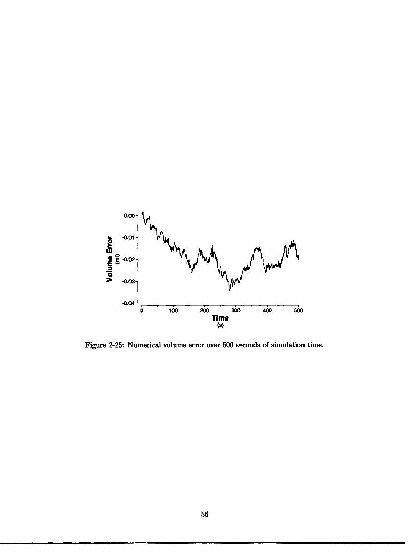
0.00-

-0.01 -

wEE -0.02-

> -0.03-

-0.04-10oo 200 300 400 500

Time(s)

Figure 2-25: Numerical volume error over 500 seconds of simulation time.

56

Chapter 3

Cardiovascular Control System

The cardiovascular system is responsible for supplying the tissues and organs of thebody with the oxygen and other nutrients required for their metabolic needs; its timelyresponse to hemodynamic perturbations or to changing metabolic demands is criticalfor an individual's optimal performance and even survival. To accomplish its task, thecardiovascular system relies on the combined effect of global reflex mechanisms thatregulate central hemodynamic variables and local control that modulates regionalblood flow in response to changing metabolic demands or to hemodynamic stresses.At either level, the cardiovascular system can recruit a hierarchy of reflex mechanisms,each having different temporal responses, to cope both dynamically and adaptivelywith a large variety of stresses.

In modeling the cardiovascular control mechanisms relevant to the short-termhemodynamic response to orthostatic stress, we focus on representing the two ma-jor neurally-mediated reflex mechanisms, namely the arterial baroreflex, discussed inSection 3.1, and the cardiopulmonary reflex, described in Section 3.2. It will be shownin subsequent chapters that the hemodynamic effects associated with sudden ortho-static stress are quite dramatic so that the neurally-mediated global reflex responsesare likely to dominate the immediate circulatory response.

3.1 Arterial Baroreflex

The arterial baroreflex is the most potent guardian of short-term blood pressurehomeostasis on the high-pressure side of the circulation; when required, its actionscan develop full strength well within a few seconds, allowing for a rapid and decisiveresponse to sudden hemodynamic stress. Hard-wired neural pathways connectingarterial pressure sensors to effector organs account for this responsiveness.

The afferent limb of the arterial baroreflex consists of stretch receptors in thearterial wall of the aortic arch and the carotid sinuses, and neural pathways con-necting them to the central nervous system. The receptors respond to changes inarterial transmural pressures by changing their rate of depolarization; hypertensivestimuli lead to an increased rate of depolarization whereas hypotensive stimuli havethe opposite effect. The resultant electrical impulses propagate via afferent nerve

57

Figure 3-1: Diagrammatic representation of the cardiovascular control model. APAA(t),

APcs(t), APRA(t): aortic arch, carotid sinus, and right atrial transmural pressures.

fibers traveling alongside the glossopharyngeal nerves (carotid sinus reflex) and vagusnerves (aortic arch reflex) to converge on the nucleus tractus solitarius (NTS), a ma-jor functional center of autonomic activity in the medulla oblongata. Afferent nervetraffic is thought to have direct inhibitory influence on the NTS, leading to reciprocaleffects on the two efferent limbs of the autonomic nervous system: increased afferentnerve traffic reduces efferent sympathetic outflow and increases efferent parasympa-thetic action. The sympathetic (thoracolumbar) division of the autonomic system isformed by visceral efferent fibers originating from the thoracic and lumbar portionsof the spinal cord. At its nerve terminals, the sympathetic nervous system releasesnorepinephrine, which acts via P,-sympathetic receptors in cardiac tissue to increaseheart rate and cardiac contractility, and via al-sympathetic receptors found in themuscular wall of arterioles and veins to constrict vascular smooth muscle (increasingarteriolar and venous tone). The latter leads to an increase in arteriolar resistance anda decrease in venous zero pressure filling volume. The parasympathetic (craniosacral)division of the autonomic system consists of cranial nerves III (occulomotor), VII (fa-cial), IX (glossopharyngeal), and X (vagus), and spinal nerves S2-4. Of cardiovascularinterest, however, are primarily the vagus nerves that convey efferent signals to theheart and abdominal viscera. The parasympathetic system releases acetylcholine, arapidly-metabolized neurotransmitter, which acts on the heart primarily by slowingits rate and on the peripheral vasculature by dilating arterioles and venules.

In Figure 3-1 we give a diagrammatic representation of the major functional-ana-tomical components of the neural reflex loops just described for the arterial baroreflex.

58

3.1.1 Architecture of the ModelIn consonance with previous work [11, 31, 140], we model the arterial baroreflex asa set-point controller that aims at minimizing an error signal, namely the deviationof (local) time-averaged arterial pressure from a pre-defined set-point value, by ad-justing various effector mechanisms in a feedback configuration. As will be shown,this set-point model is quite powerful in representing the short-term cardiovascularcontrol mechanisms; yet it is also quite abstract in that its functional elements donot necessarily map to any of the functional-anatomical components described aboveand depicted in Figure 3-1.

The hemodynamic model described in the previous chapter generates samples ofaortic arch, APAA(t), and carotid sinus transmural pressures, Pcs(t), at a rate de-termined by the numerical integration stepsize (dt 10-3 S). As pointed out byMukkamala [141], pulsatile arterial blood pressure is band-limited to frequencies be-low ten times the mean heart rate, while the frequency responses of the autonomicallymediated cardiovascular reflex mechanisms are band-limited to frequencies less thanthe mean heart rate. Relaying every pressure sample to the reflex system is there-fore neither computationally advisable nor physiologically necessary. Consequently,as indicated in Figure 3-2, the first processing step on the afferent side involves av-eraging of the arterial pressure waveforms over an appropriate window of time. Weemploy a moving average filter over the recent 0.25s arterial pressure histories andadvance the filter every 0.0625 s to generate samples of the respective averaged values,APAA[n ] and aPcs[n], at a rate of 16 Hz. The discrete-time index n is used to indi-cate their relatively coarse sampling compared to the actual pressure waveforms. Weimplemented the averaging process via backward Euler integration which delays theoutput by approximately 0.125 s; we will compensate for this delay when consideringthe overall time delay of the reflex responses.

Instead of modeling the aortic and carotid sinus reflex loops separately, we adopteda hybrid strategy in which we assume the input to a single, lumped arterial barore-ceptor to be the arithmetic mean APA[n] of APAA[n] and APcs[n]. Given the relativepaucity of experimental data on the aortic baroreflex, this averaging strategy allowsus to maintain the differential influence these receptors exert during respiration orchanges in posture, for example. Quite conceivably, though, the equal weighing of

Pref

aPcs(t)

APAA (t)

Figure 3-2: Arterial baroreflex model: functional representation of afferent and centralnervous pathways.

59

xo

6PA[n] - X[n]

AXCcp[n]

Figure 3-3: Arterial baroreflex model: functional representation of central nervous andefferent processing for an effector variable X.

aortic arch and carotid sinus transmural pressures might be a strong assumption tomake, particularly in situations when one set of receptors senses a substantially dif-ferent signal than the other. We will revisit this assumption when simulating thetransient response to orthostatic stress.

To generate an error signal, PA[n], we subtract a pre-defined arterial set-pointpressure, PAef, from the lumped arterial pressure APA[n], and scale the resultant signalas described by deBoer and co-workers [140]:

PA[n] = 18 arctan ((PAA[n] + aPcs[n]) PAf (3.1)

to account for the experimentally-observed sigmoidicity of the stimulus-response curves[142]. This scaling limits the error signal to approximately ±28 mm Hg.

Figure 3-3 illustrates the efferent side of the arterial baroreflex, where the errorsignal is convolved with unit-area impulse response functions, sx[n] and px [n], andscaled by static gain values, Gx and GP, to determine the arterial baroreflex contri-bution, aXA[n], to the current value of the effector variable X[n]. For completeness,we also show the effector set-point, X 0, and the additive contributions of the car-diopulmonary reflex loop, aXcp[n], to X[n]. Here X denotes any of the four effectormechanisms illustrated in Figure 3-1. G and GP represent the sympathetic andparasympathetic static gain values; sx[n] and px[n] denote the sympathetic and theparasympathetic unit-area impulse response functions associated with the effectormechanism represented by X.

In the case of the arterial resistance and the venous tone effector limbs, thediscrete-time values of X[n] are linearly interpolated to allow for smooth variationof the effector variables R(t) and Vo(t). Interpolation requires that both X[n] andX[n + 1] be available at time t, which introduces a delay of 0.0625s for these twoeffector loops.

As described in Section 2.2, the cardiac capacitances vary throughout the car-diac cycle between an end-systolic and a diastolic value. The contractility feedbackaffects the respective end-systolic values, Cr[i] and Crl[i]. Here, we introduced thediscrete-time index i to denote beat number and to emphasize explicitly the beat-by-

60

0N

.-3

v.W

N

Itf% ek.0 V

I I I I I I I I

-40 -20 0 20 40Time (sec)

l a_

I I I I I I I I

-40 -20 0 20 40Time (sec)

Figure 3-4: Parasympathetic (top) and sympathetic (bottom) canine heart rate impulseresponse functions. Adapted from Berger et al. [144].

beat nature of variations in contractility as opposed to the smooth variation of R(t)and Vo0(t). We implemented the contractility feedback via a sampled-data model inwhich the reflex signals Ces,[n] are sampled at times t[i], corresponding to the onsettimes of cardiac contraction, to establish the end-systolic capacitance values Cl[i]for the ensuing beat. The onset times t[i] are determined via an Integral Pulse Fre-quency Modulator (IPFM) model of the sino-atrial node. The latter will be discussedin detail in Section 3.3 where we describe the heart rate limb of the arterial baroreflex.

In summary, the arterial baroreflex is described by a single arterial set-point, PAf,and possibly two static gain values and two normalized impulse response functionsfor each effector mechanism. The assignment of numerical values to these parametersis the topic of the following section.

3.1.2 Parameter Assignments

Impulse response functions By directly stimulating the stellate ganglia (sym-pathetic stimulation) and the vagus nerves (parasympathetic stimulation), Berger[143, 144] identified the canine heart rate impulse response functions for parts ofthe efferent neural pathways and the sino-atrial node. The impulse response func-tions so identified are reproduced in Figure 3-4 and confirm common physiologicalknowledge that vagal stimulation leads to an immediate decrease in heart rate andsympathetic stimulation to an increase over slightly longer time scales. In fact, theparasympathetic impulse response function attains nonzero values before the onset ofvagal stimulation (at time zero), suggesting a non-causal heart rate response. Berger[143, p. 133] considers this an artifact of the particular signal processing algorithmsemployed. More importantly, though, the impulse response functions shown in Fig-

61

___ _ __ _ ___ I_____ _______

0

ure 3-4 characterize contribution of the end-organ response and the efferent neuralpathways only, omitting the contributions of the receptors, the afferent pathway, andthe central nervous system. For pure reflex responses, the latter contributions aredescribed as pure delay elements in series with the former contributions [11]. Thetriangular shapes of the impulse response functions suggest a parameterization interms of three timing variables (a delay, a peak, and an end-point). These idealizedresponses will serve as prototypes for the impulse response functions to be developedfor other effector organs.

Having had access to a unique study population, Borst and Karemaker [145] wereable to study the latencies of the human arterial baroreflex by directly stimulatingthe carotid sinus nerves in eleven subjects. Looking at P-P-interval changes, theydetermined a delay of 0.5-0.6 s for vagally mediated heart rate control. Furthermore,by pacing the heart at a fixed rate while stimulating the carotid sinus nerves, theydetermined the delay of the a-sympathetic response to arterial resistance to be 2-3 s.

Several investigators have used periodically varying external neck pressure to stim-ulate the carotid sinus and thus to elucidate human baroreflex dynamics noninvasively[146-148]. Eckberg found a 0.44 s delay for vagally mediated heart rate control in re-sponse to reductions in carotid sinus transmural pressure. Keyl and co-workers [148]found this delay to be (0.59 ± 0.25) s. We adopt Keyl's value for the delay and followDavis' choice for the peak and the end point of the parasympathetic impulse responsefunction [11]. Furthermore, we assign Keyl's estimate of the degree of variability inthe delay to all three of the parasympathetic parameters.

Rea and Eckberg [147] measured muscle sympathetic nerve activity at the peronealnerve in response to changes in external neck pressure. Their data suggest a delay ofat least 2.8 s for a-sympathetically mediated reflex responses which is congruous withthe data presented by Borst and Karemaker. We assume this delay to be (2.5 i 1.0) s.

Due to experimental difficulties, little direct experimental evidence exists for thelatencies of the /-sympathetic heart rate response or the a-sympathetic responseof venous tone in humans. For dogs, Berger noted that the -sympathetic filtercharacteristics shown in Figure 3-4 closely match the results reported by Rosenbaumand Race [149], who studied the canine vascular resistance response. He suggestedthat this commonality reflects universal kinetic properties of adrenergic receptors andtheir cellular signaling mechanisms. Studying venous tone feedback in dogs, Shoukasand colleagues [150] observed a significantly longer delay ( 10s) than the onesreported by Berger and Rosenbaum. We assume the delays of the /-sympatheticheart rate response and the a-sympathetic arterial resistance response to be equal,but we assume a slightly longer delay for the a-sympathetic response of venous toneas indicated in Table 3.1.

Using system identification techniques, Mullen and co-workers [151] investigatedclosed-loop cardiovascular regulation. While they do not separate parasympatheticand -sympathetic responses, it is safe to assume that the tail of their impulse re-sponse function is primarily sympathetically mediated, which would suggest an end-point for the 3-sympathetic response at around (15.0 ± 5.0) s. Mukkamala [152],from the same laboratory, investigated the human arterial resistance response to stepchanges in arterial pressure. His data suggest the peak of the impulse response occurs

62

Table 3.1: Parameterization of the reflex impulse response functions

Type of Response Delay Peak Ends s s

parasympathetic (0.59 + 0.25) (0.70 + 0.25) (1.0 i 0.25)/-sympathetic (2.5 ± 1.0) (3.5 t 1.0) (15.0 ± 5.0)

a-sympathetic to R (2.5 i 1.0) (4.5 + 1.0) (30.0 + 5.0)a-sympathetic to Vo (5.0 + 1.5) (7.0 ± 1.5) (40.0 ± 5.0)

approximately 2 s after the onset of the reflex response. Furthermore, the responseseems to equilibrate 30 s after the stimulus was applied. Finally, we assume slightlylarger values for the peak and the end-point of the a-sympathetic response to venoustone.

In assigning a single impulse response function to each effector arc, we neglect acommonly reported experimental finding that the arterial baroreflex responds fasterto hypertensive stimuli (average parasympathetic delay 0.26 s) than to hypotensivestimuli (average parasympathetic delay 0.44s) [146, 153]. Where possible, weselected the timing information associated with hypotensive stimuli, as this is theprincipal focus of this work.

Finally, we sample the impulse response functions at 0.0625 s and implement themadvanced in time to account for the delays introduced by the averaging filter andinterpolator described in the previous section.

Static gain values While it would be desirable to determine the open-loop gainsof each of the four effector mechanisms independently, such experiments are tech-nically very difficult in conscious animals and ethically not permissible in humans.Determination of gain values is therefore commonly based on the closed-loop systemin which perturbations in systemic arterial blood pressure are induced pharmacolog-ically or the carotid sinus is stimulated mechanically while the reflex responses ofcertain effector mechanisms are being observed.

Several studies induced hypertension through bolus-administration of potent vaso-constrictor agents, such as phenylepherine or angiotensin, while the ensuing reflexbradycardia was observed to quantify the stimulus-response curve of R-R-intervalto changes in blood pressure [154-158]. Studying 23 normal control subjects, Eck-berg and co-workers [155] determined this gain value to be (16.0 i 8.6) ms/mm Hgwith a range of (5.0 - 35.0) ms/mm Hg. Bristow and colleagues [154] report (14.8 ±9.2) ms/mm Hg with a range of (3.6 - 29.3) ms/mm Hg while Pickering [157] quotes asomewhat higher value of (30.0±4.0) ms/mm Hg with a range of (13.3 - 48.7) ms/mm Hg.Pooling the data from these three studies results in an average R-R-interval gainvalue of (22.7 ± 9.5) ms/mm Hg with a range of (3.6 - 48.9) ms/mm Hg. We followdeBoer's [159] suggestion of dividing the gain equally between the sympathetic andthe parasympathetic reflex arcs.

Little quantitative information is available on the reflex changes of cardiac con-

63

Table 3.2: Static gain values of the arterial baroreflex model

Reflex arc Gs GP

R-R-interval mmg (11 + 6) (11 6)

Left ventricular ml (0.007 0.001) 0contractility mm (0.007 0.001) 0

Right ventricular ml (0.022 0.003) 0contractility mm Hg

Arterial resistance PRg (-0.05 i 0.01) 0

Venous unstressed ml (31 5) 0volume mmHg

tractility. Following Davis' reasoning [11], we allow the right and left ventricularend-systolic elastances to attain between 170% and 210% of their respective nominalvalues in response to maximal carotid sinus stimulation. This translates to gain val-ues of (0.007 ± 0.001) ml/mm Hg2 and (0.022 ± 0.003) ml/mm Hg2 for the end-systoliccapacitance of the left and the right ventricle, respectively.

Under high orthostatic stress, the cardiovascular system is capable of doublingtotal peripheral resistance [160, 161]. If we assume that in the limit of life-threateninghypotension, peripheral resistance can be increased to 2.5 - 3.0 PRU, and that thisresponse is overwhelmingly mediated by the arterial baroreflex, we obtain an upperlimit for the peripheral resistance gain value of (0.05 - 0.07) PRU/mm Hg. We assigna value of (0.05 ± 0.01) PRU/mm Hg and assume each of the systemic vascular bedsto contribute equally.

Reflex-induced changes in venous unstressed volume are difficult to quantify inhumans due to our inability to measure venous volumes directly. Under maximalcarotid sinus stimulation, dog experiments have revealed a maximum change in sys-temic reservoir volume of approximately 12 ml/kg, 6-7 ml/kg of which originate fromabdominal vessels [162]. When scaled to a 75 kg human, these data suggest a maximalchange in venous unstressed volume of about 900 ml and imply a static gain valueof 31 ml/mm Hg, given the limitation of the afferent signal of the arterial barore-flex model. We attribute (15 ± 3) ml/mm Hg to the splanchnic venous reservoir,(8 ± 2) ml/mm Hg to the lower body, (6 ± 2) ml/mm Hg to the upper body, and(2 ± 1) ml/mm Hg to the kidneys. The static gain values for the arterial baroreflexmodel are summarized in Table 3.2.

Finally, we assign the value of 91 mm Hg to the set-point pressure of the arterialbaroreflex.

64

3.2 Cardiopulmonary Reflex

Neurogenic reflex mechanisms originating from the low pressure side of the circulationand the heart were first described around the same time as their arterial analogs. To-day, their role in neurohumoral control of cardiovascular function and fluid-electrolytebalance is hardly questioned; yet their physiological significance in short-term cardio-vascular homeostasis is still being debated.

Cardiopulmonary receptors located in the atrio-caval junctions, the atrial and theventricular walls, and even in the pulmonary vasculature are commonly divided intoA-type receptors (mechano-receptors) and B-type receptors (stretch receptors). Af-ferent signals from these receptors travel along vagal fibers and converge on vagalcenters in the medulla oblongata. Cardiopulmonary stimulation is thought to havedirect inhibitory influence on medullary vasoconstrictor centers, leading to reciprocaleffects on parasympathetic and sympathetic outflow: increased afferent nerve trafficreduces efferent sympathetic outflow and is thought to increase efferent parasympa-thetic action.

The cardiopulmonary reflex also exerts important longer-term neurohumoral con-trol over cardiovascular function. Direct cardiopulmonary influence on vasopressin(antidiuretic hormone, ADH) and atrial natriuretic peptide (ANP) release allows forlow-pressure modulation of renal fluid-electrolyte balance.

Finally, cardiopulmonary-mediated vagal outflow has long been thought to con-tribute to, if not be causative of, vasovagal syncope during prolonged orthostatic stressor hemorrhage; it is associated with a triad of cardiopulmonary responses (bradycar-dia, hypotension, and apnea) commonly referred to as Bezold-Jarisch reflex.

The architecture of our cardiopulmonary reflex model is quite similar to the onedescribed for the arterial baroreflex. The sensed variable is right atrial transmuralpressure, APRA(t). After averaging and subtraction of the cardiopulmonary set-pointpressure, Pcpf, the scaled error signal SPcp is computed according to:

Pcpn = 5 arctan cp [n] -P er (3.2)

The efferent processing steps are again similar to the arterial baroreflex in thatthe error signal is convolved with unit-area impulse response functions and scaledby effector mechanism-specific static gain values to produce the cardiopulmonarycontribution, aXcp [n], to the current value of the effector mechanism X (see Figure 3-3). We also assume the timing of cardiopulmonary control to be described by thesame impulse response functions identified in the previous section. What remains tobe established, therefore, are the static gain values for the various reflex limbs.

Cardiopulmonary control of heart rate is commonly known under the eponym ofBainbridge reflex. It states that right atrial distention leads to a reflex tachycardiamediated by cardiopulmonary receptors [163, p. 89]. While the Bainbridge reflexhas been amply documented in canine experiments, its physiological significance,or even its existence in humans has been questioned. As reviewed by Mark and

65

Table 3.3: Static gain values of the cardiopulmonary reflex model.

Reflex arc Gs GP

Arterial resistance PRu (0.05 ± 0.01) 0mm Hg

Venous unstressed ml (100 ± 20) 0volume mmHg

Mancia [164], increasing right atrial pressure in humans through infusion of volumeor raising of the legs fails to show the reflex tachycardia seen in dogs with right atrialdistention. Furthermore, copious lower body negative pressure experiments confirmthat reductions in right atrial pressure fail to elicit a heart rate response until changesin arterial pressure become evident [165, 166]. In a recent study, Desai and co-workers[167] tried to untangle the contributions to the cardiac period of cardiopulmonary,aortic arch, and carotid sinus receptors. Their analyses suggest not only a positivegain value connecting right atrial pressure to R-R-interval (i.e. an inverse Bainbridgereflex), but also that the strength of this coupling is an order of magnitude largerthan the influence of carotid sinus pressure on the cardiac period. Given the lack ofunequivocal experimental support for a Bainbridge reflex in humans, we decided toset the static gain values for the coupling of right atrial pressure to R-R-interval tozero, i.e. we neglect the Bainbridge reflex. Similarly, we do not account for a possibleinfluence of right atrial pressure on cardiac contractility, given that such a couplingis negated in animal experiments [163, p. 89].

Cardiopulmonary contributions to peripheral resistance feedback can be estimatedfrom LBNP experiments. Low levels of LBNP usually elicit a vasoconstrictor responsewithout increases in heart rate maintaining stable arterial pressures [165, 166]. Thedata presented by Pawelczyk and Raven [166] suggest a static gain value of 0.05 -0.06 PRU/mm Hg for the cardiopulmonary - peripheral resistance reflex limb, a valueconspiciously similar to the one found for the arterial baroreflex.

Experiments in humans have shown splanchnic blood volume to change by ap-proximately 500 ml in response to a 1000 ml hemorrhage without significant changesin heart rate, cardiac output, and arteriolar resistance [168]. Assuming this responseto be mediated by the cardiopulmonary reflex only, we can get a rough estimate ofthe cardiopulmonary reflex gain to venous tone by assuming that the contributionof the splanchnic circulation is about 60 % of the total venoconstriction response.These assumptions would suggest a static venous tone feedback gain of approxi-mately 100 ml/mm Hg as the cardiopulmonary afferent pressure signal is limited to :8 mm Hg. A significantly larger gain value for venous tone feedback on the low pres-sure side as compared to the analogous gain value of the arterial baroreflex might beexplained teleologically by the importance of the venous reservoir to maintain cardiacfilling pressure via the Frank-Starling mechanism.

While neurohumoral control of the cardiovascular system plays a significant role

66

Ii!i 00 mose

Figure 3-5: Intracellular recording of pace- Figure 3-6: Schematic representation of howmaker activity recorded within the morpho- changes is pacemaker properties lead to car-logical boundary of the rabbit SA node [170, diac deceleration. Adapted from [171].

p. 93].

in adaptation to prolonged orthostatic stress, its importance to short-term cardio-vascular control is questionable. Several studies confirmed that humoral mediators,such as renin, aldosterone, and vasopressin, only attain significant plasma concentra-tions after 10-15 minutes of sustained orthostatic stress [36, 169]. We therefore ignoreneurohumoral control in this work.

Finally, we assign the value of 5 mm Hg to the set-point of the right atrial trans-mural pressure.

3.3 Cardiac PacemakerIn the healthy heart, cardiac excitation is initiated when specialized cells in the sino-atrial (SA) node depolarize spontaneously - a phenomenon referred to as automatic-ity of the cardiac pacemaker cells. Due to a progressive increase in cell membranepermeability to sodium and calcium ions during the diastolic portion of the cardiaccycle, the transmembrane potential rises until a cell-specific threshold potential iscrossed, at which point the cell membrane rapidly reverses polarity and an action po-tential is generated (see Figure 3-5). Once generated, the action potential propagatesalong the cardiac conduction system to reach individual myocardial fibers, where de-polarization then leads to a rapid increase in intracellular calcium and ultimatelymyocyte contraction.

In the absence of external influences, the rate of spontaneous depolarization isconstant [172]. In the intact circulation, however, the SA node is richly innervated bysympathetic and parasympathetic nerve fibres whose balanced influence modulatesthe rate at which action potentials are being generated. Dominance of parasym-pathetic influence decelerates impulse generation and therefore reduces heart rate;a shift in autonomic balance to sympathetic dominance accelerates action potentialgeneration and therefore increases heart rate. Figure 3-6 shows schematically howcardiac deceleration can be achieved by increasing the threshold potential, th, atwhich an action potential is generated (A), decreasing the slope of diastolic depolar-

67

\ \ I ~ L~~~M 1IY | l

ization (B), or by decreasing the diastolic resting potential, .min, (C) [173]. Reversalof these parameter changes lead to cardiac acceleration.

In modeling the cardiac pacemaker we are interested in generating a sequenceof point events, namely the onset times of cardiac excitation corresponding to thethreshold-crossing of the transmembrane potential, based on a representation of au-tomaticity and the time-continuous history of neural input to the cardiac pacemaker.We have modified the approaches taken by Hyndman and Mohn [173] and laterde Boer and co-workers [159] who have used an Integral Pulse Frequency Modula-tor (IPFM) model to represent the dynamics of the transmembrane potential duringdiastole. The model is based on the idea that the transmembrane potential can berepresented as a function M(t) whose value at time t depends on the cumulative con-tribution of automaticity and autonomic activity since the onset of the last cardiacexcitation at time tk-l:

M(t) = m(t')dt'

The function m(t) can be expressed as m(t) = mo + mr(t) to represent the auto-maticity, mo, and neural (reflex) input, mr(t). The k-th beat is initiated at time tkwhen the value of the integral reaches a predefined threshold F, corresponding to thethreshold potential 4th, and the absolute refractory period of the cardiac pacemakercell has passed

ti

m(t')dt' = M(tk) > r and tk - tk-1 0.2. (tk - tk-2)-

where we assumed an absolute refractory period of one fifth of the preceeding cardiaccycle length. Once this condition is met, the function M(t) is reset and the inte-gration process is repeated. We assume m0 to be constant, which leads to a strictlyperiodic signal at a rate of mo/r in the absence of neural influence (mr(t) = 0).The neural contribution can increase (m,(t) > 0) or decrease (m,(t) < 0) the rate ofbeat generation, corresponding to sympathetic or parasympathetic dominance of theefferent autonomic signal, respectively. Neural control of heart rate in this represen-tation therefore modifies the slope of diastolic depolarization, which corresponds toMechanism B in Figure 3-6.

The reflex system supplies us with a natural choice for the function m(t), or itsdiscrete-time analog m[n], namely the inverse of the instantaneous R-R-interval I[n],

1 k=N[n] k=0m[n] = where I[n] = + Be 6PA[n-k] * (GP*p[k]+Gs*s[k])

In the absence of neural control, m[n] reduces to the constant 1//, the inverse of theset-point R-R-interval. Increased sympathetic outflow is characterized by a negativeconvolution integral (corresponding to m[n] > 1/Io) whereas parasympathetic domi-nance leads to a positive convolution integral (corresponding to m[n] < 1/Io). In thisrepresentation of m[n], the constant r is equal to 1.0.

68

Chapter 4

Model Validation

Having detailed the architecture of and the parameter assignments for the cardiovas-cular model in the previous two chapters, we now turn our attention to its predictionsand their comparison with experimental data.

A word on method: We assigned most parameter values on the basis of litera-ture reviews of largely unrelated clinical studies, so we cannot expect the resultantmodel to generate cardiovascular data in uniform agreement with a large variety ofexperimental observations without adapting some of the parameter values. We willtherefore find it necessary to adjust a small number of model parameters to matchcertain key variables for each set of comparisons. We refer to this step as ModelCalibration and will provide the reader with a clear rationale in each case as to whycertain parameters need to be adjusted. We chose the term Model Calibration toemphasize its difference from Model Optimization. The latter term will be reservedfor a strategy to search for parameter values that optimally (by some quantitativemeasure) represent a given data set in its entirety. Model Optimization is the topicof Chapter 6.

In Section 4.1 we illustrate the closed-loop operation of the model by quantitativelycomparing various blood pressure and blood flow numerics to data reported in healthyrecumbent subjects. Section 4.2 expands the scope of the simulations to represent notone typical member of a population of normal subjects but to represent the populationitself. In Sections 4.3 and 4.4, we compare to experimental data the steady-state andthe transient simulated hemodynamic responses of head-up tilt, standing up, andlower-body negative pressure. The simulation of rapid-onset exercise is the focusof Section 4.5; while this topic is not central to the thesis, it does demonstrate theversatility of the developed model. We close this chapter with some remarks aboutthe forward model.

4.1 Baseline SimulationAs pointed out in Section 2.1.2 (p. 28), we assigned parameter values with the goalof representing the cardiovascular state of normal, healthy subjects. We also notedthat whether or not we achieved this goal can only be judged once the parameter

69

Table 4.1: Steady-state hemodynamic variables of normal recumbent adults. Comparisonof simulations and experimental data.

Simulations Measurements

Uncalibrated Calibrated Meant Range

Pressures, mm Hg

Radial arterytSystolicMeanDiastolic

Peripheral veinMean

Right atriumMean

Right ventricleSystolicEnd-diastolic

Pulmonary arterySystolicMeanDiastolic

Pulmonary capillary wedge*MaximumMeanMinimum

Left atriumMean

Left ventricleSystolicEnd-diastolic

988877

9

2

21

1

201510

1049177

9

2

241

221610

12109

13108

4

1008

5

1068

(135 ± 15.7) (106-164(91 + 8.7) (75-110(71 ± 7.4) (64-86)

(8 ± 2.5) (4-13)

(0 1.6) (-2-2)

(25 + 3.4) (18-30)(2.6 + 1.4) (-0.5-4.5

(22 + 3.7) (13-30)(17 + 3.1) (10-21)(12 : 2.6) (3-15)

(15 ± 2.9) (8-23)(12 i 2.0) (8-15)(9 9 2.2) (5-14)

(7.9 ± 3.0) (2-12)

(118 16) (90-140(8.7 ± 2.3) (5-12)

4)

5)

)

Left ventricular end-diastolicvolume index, ml/m 2

Left ventricular end-systolicvolume index, ml/m 2

Cardiac index, I/min/m2

Stroke index, ml/beat/m 2

Heart rate, beats/min

62 72

32

2.4

33

2.9

30

80

39

75

(70±20) (54-120)

(24±10) (14-45)

(3.5 ± 0.7) (2.5-5.3)

(46 + 8.1) (37-72)

(79 ± 13.8) (59-113)

Systemic resistance, PRU 1.17

tMean ± population standard deviation.*Compared to pulmonary venous pressure.

1.02 (0.85 ± 0.17) (0.56-1.18)

tCompared to aortic root pressure.

70

---

values have been assigned, the model assembled, and its predictions compared toexperimental data. Such comparison is the topic of this section.

Using the parameter profile and the general architecture of the hemodynamic andthe reflex models, we can generate pressure, flow, and volume waveforms from whichwe can extract beat-to-beat numerical measures of cardiovascular variables. Under thecolumn title "Simulations - Uncalibrated" in Table 4.1, we summarize steady-statenumerics for variables commonly used clinically to assess a subject's cardiovascularstate, and compare them to measurements reported for healthy recumbent volunteersunder resting conditions [60, 174-178]. The model-derived pressures generally tend toagree with the mean values reported for the normal population. The values derived forstroke volume, cardiac output, and systemic vascular resistance, however, lie outsidethe range for the normal population and suggest a strategy for refinement of someparameter values.

It seems that these deviations can be reconciled by lowering systemic vascularresistance and increasing the diastolic compliances of the left and right ventricles.The former leads to an increase in venous return whereas the latter enhances car-diac output. Referring to Table 2.4, we note that a reduction of each systemic mi-crovascular resistance by 0.5 PRU is compatible with the normal degree of variabilityof these parameters. Similarly, diastolic ventricular compliances of approximately20 ml/mm Hg and 9 ml/mm Hg for the right and the left heart, respectively, are inagreement with experimental findings (see Table 2.7). Finally, we increase the set-point of the cardiopulmonary reflex loop by 1 mm Hg to maintain mean right atrialtransmural pressure at 6mmHg. In the second data column of Table 4.1, we sum-marize the simulation results using this slightly altered set of parameter values. Thediscrepancies between simulations and clinical results pointed out previously havebeen reduced.

The discrepancies between systolic and diastolic radial artery pressure measure-ments and their simulated equivalents point to an interesting limitation of the lumped-parameter hemodynamic model, namely its inability to reproduce phenomena thatarise as a result of the distributed nature of the cardiovascular system. The exampleat hand is the well-known phenomenon that the morphology of the arterial pressurewaveform changes significantly as a function of location within the arterial system:while mean arterial pressure decreases slightly, peak-systolic pressure increases anddiastolic pressure decreases the further distal from the heart the pressure is beingmeasured [see, e.g. 179, p. 176]. This behavior has been linked to the geometric non-uniformity of the arterial system [180, p. 134]. In particular, it has been attributedto changes in the vascular impedance that occur along the arterial system at branch-ing points, at the terminal arterioles, and also along the gradually tapered arterialvessels [181]. Measurements reported from a single subject suggest pulse pressure toincrease by about 40 % between the aortic root and the femoral artery [179, p. 176].Since the effect of taper diminishes in the proximal direction, it is the arterial systolicand diastolic pressure at the root of the aorta that is approximated by our lumpedparameter representation.

Furthermore, the lack of inertial effects is evident in Figure 4-1 as the central

71

120

10

I 40

I

P4 icur prune

JP PUhtry

L~~~ I~~I~~PUUMIDB - & - O R - b h t dd~~~~~~~~10rM-% '-- .J-

0.0 0.5 1.0 1.5 2.0 0.0 05 10 lb 2.0

Tl Time T

Figure 4-1: Simulated pressure waveforms of the left heart and systemic arterial system(left) and the right heart and the pulmonary artery (right).

arterial and pulmonary arterial waveforms lack the dichrotic notch expected to oc-cur during closure of the semi-lunar valves. Apart from these morphological finestructures, the model represents atrial, ventricular, and peripheral waveforms well.

The analysis so far has centered around the steady-state values of certain car-diovascular variables. In order to probe the dynamic behavior of the cardiovascularmodel, we need to allow for perturbations of its normal operating conditions. In thesections to follow, we will introduce sudden orthostatic stress as such a challenge tothe system. Here, we simply note that the model's response to a simulated Valsalvamaneuver reproduces the typical response seen experimentally. Both experimentaldata and simulations are shown in Figure 4-2, where we simulated the Valsalva ma-neuver by increasing intra-thoracic and intra-abdominal pressures by 40 mm Hg for aperiod of 30 s after which the pressures are returned to their normal values.

130-

110.

' 0O

I .a I- E 10-

110

70

0-

7o-

60-

50- * .50--10 0 10 20 S0 4 50 -10 0 10 20 io 0 0

Mm knh() (Ma)

Figure 4-2: Heart rate and arterial blood pressure response to a Valsalva maneuver. Top:simulation result; bottom: experimental recording from one subject.

72

0-

go.

go.

70-

M.

4.2 Population Simulations

The simulations presented in the previous chapter demonstrate that the model iscapable of reproducing average cardiovascular variables. Here, "average" refers tothe population against which the model response is compared. In this sense, themodel framework forms a valid representation of the average cardiovascular state ofa healthy population.

Rather than simulating the mean response of a population, a more powerful ap-proach would be to simulate the responses of individual members of the population.On the basis of these responses, one could calculate any desired summary statistic,such as the mean or median response along with their degree of variation. Such anapproach presupposes access to a large number of parameter profiles representing thecardiovascular states of the individual members. We could establish such profilesby retracing the arguments presented in Chapters 2 and 3, assuming different an-thropometric and cardiovascular variables. This approach would be quite laborious.Instead, we combine the nominal set of parameter values and their standard errorswith general allometric scaling laws to generate parameter profiles of subjects withdifferent anthropometric and cardiovascular characteristics. The details of this ap-proach would detract from the theme of this chapter and are therefore presented inAppendix B.

In Table 4.2, we summarize the anthropometric profile of the sampling populationbased on 500 realizations of the sampling scheme outlined in Appendix B. Table 4.3,presents the population statistics of the numerical cardiovascular measures presentedpreviously in Table 4.1. The data demonstrate that in addition to the mean values,the degrees of variability and the ranges of the population-based simulations generallymatch their experimental analogs quite well.

Looking ahead, we note that failure of the cardiovascular system to adjust properlyto the upright posture is commonly associated with high heart rates and low strokevolumes. We therefore paid particular attention to validating the model's baselinestroke volume and cardiac output and their response to changes in heart rate. InFigure 4-3, we reproduce the data reported by deSimone and co-workers [62] whostudied normalized cardiac output as a function of body weight in children and adults.Our simulations represent adult cardiovascular physiology only and therefore lack thepart of the distribution representing children and adolescents. The distribution of

Table 4.2: Anthropometric profile of simulated population.

Height Wei Body SurfaceHeight Weight AreaArea

cm kg m2

Mean (169 i 9.1) (70 ± 14.0) (1.84 ± 0.21)Range (144-202) (42-117) (1.38-2.56)

73

Table 4.3: Comparison of population simulations to steady-state hemodynamic variables ofrecumbent adults.

Simulations MeasurementsVariable Meant Range: Meant Range

Pressures, mm Hg

Radial artery*Systolic (107 ± 7.5)Mean (94 4 5.1)Diastolic (79 ± 3.4)

Peripheral veinMean (10 ± 2.8)

Right atriumMean (2 ± 1.7)

Right ventricleSystolic (24 i 5.9)End-diastolic (1 + 2.0)

Pulmonary arterySystolic (23 4 6.0)Mean (17 i 4.4)Diastolic (11 ± 3.5)

Pulmonary capillary wedge*Maximum (13 + 3.4)Mean (10 i 2.8)

Minimum (9 ± 2.6)Left atrium

Mean (5 2.5)

Left ventricleSystolic (108 ± 7.7)End-diastolic (8 ± 2.8)

(97-120)(86-103)(74-85)

(6-15)

(0-5)

(15-35)(-1-4)

(13-34)(10-24)(8-17)

(8-20)

(7-16)(5-13)

(2-8)

(98-122)(5-13)

Left ventricular end-diastolicvolume index, ml/m 2 (72 ± 14.7) (52-96)

(135 ± 15.7)(91 8.7)(71 7.4)

(8 2.5)

(0 1.6)

(25 ± 3.4)(2.6 + 1.4)

(22 i 3.7)(17 ± 3.1)(12 ± 2.6)

(15 ± 2.9)(12 ± 2.0)(9 2.2)

(106-164)

(75-110)(64-86)

(4-13)

(-2-2)

(18-30)

(-0.5-4.5)

(13-30)(10-21)(3-15)

(8-23)(8-15)(5-14)

(7.9 ± 3.0) (2-12)

(118 ± 16)(8.7 ± 2.3)

(90-140)(5-12)

(70±20) (54-120)

Left ventricular end-systolicvolume index, ml/m 2

Cardiac index, I/min/m 2

Stroke index, ml/beat/m 2

Heart rate, beats/min

(34 ± 9.8) (18-50)

(2.7 ± 0.4) (2.3-3.4)

(38 8.4) (27-51)

(74 7.8) (61-87)

(24±10) (14-45)

(3.5 ± 0.7) (2.5-5.3)

(46 ± 8.1) (37-72)

(79 + 13.8) (59-113)

Systemic resistance, PRU (1.13 + 0.19)

tMean population standard deviation.*Compared to aortic root pressure.

t(0.05-0.95) inter-quantile range.*Compared to pulmonary venous pressure.

74

(0.84-1.48) (0.85 ± 0.17) (0.56-1.18)

II2I -

Ial

o0o mo 40* a" m tU 20 40 G0 80 10

Bo* VV() Body W-G (kWg)

Figure 4-3: Normalized cardiac output as a function of body weight. Experimental data(left) and simulation results (right). Figure on the left adapted from [62].

simulated normalized cardiac output compares quite favorably to the part of theexperimental observations it represents.

In Figures 4-4 and 4-5, we reproduce data (solid circles) from an anesthetizedcanine preparation that demonstrate the effect of heart rate changes on steady-statestroke volume and cardiac output [182]. The data document a reciprocal relation-ship between heart rate and stroke volume: as heart rate increases, stroke volumedecreases monotonically, presumably due to successive shortening of the diastolicventricular filling phase of the cardiac cycle. Despite the reduction in stroke volume,cardiac output initially increases and subsequently stays relatively constant up toabout 200 beats/minute. Further increases in heart rate result in incrementally largerdrops in stroke volume and reductions in cardiac output. The latter phenomenon isprobably due to sub-optimal relative timing of atrial and ventricular contractions suchthat the contribution of atrial systolic ejection to ventricular filling volume becomesimpaired.

The solid lines in both figures are the mean simulated population responses; thedashed lines bound one standard error of the mean responses. Both simulations andexperimental data have been normalized such that the stroke volume and the cardiacoutput at 160beats/minute serve as the reference. Simulated and experimental re-sponses agree exceptionally well up to heart rates of about 210 beats/minute whenthe simulated cardiac output response fails to mimic the pronounced roll-off exhibitedby the experimental data. Several explanations seem plausible for this discrepancy.First, the ventricular systolic time interval scales with R-R-interval length accordingto V/T~j. This relationship is based on a data set not very rich at very high heartrates and might therefore overestimate the systolic and early diastolic time inter-vals in that regime [98]. Second, we have neglected completely all inertial effects ofblood flow, which implies that the cardiac chambers can fill very rapidly. Inclusionof inertial effects will hinder ventricular filling predominantly at high heart rates.

Despite these discrepancies, the model represents well cardiac output in the generalpopulation and its behavior as a function of heart rate.

75

II

..

.. ' - , Lk "M 1 .4 60- .0.

-; " " " ·-

I

jI

1.2 -

_ 1

1.0-

S 0.11

0.7-

40 e 16 120 O 160 180 Z0 22D 24D 2o 40 O10 K 120 140 O 102 0Z 20 2O

HIlt Ras HIMt RIO(beet pw mhn*) (b pW rmh)

Figure 4-4: Effect of heart rate on stroke Figure 4-5: Effect of heart rate on cardiacvolume. Simulation: mean response (solid output. Simulation: mean response (solidline) ± SE (dashed lines); solid circles: data line) ± SE (dashed lines); solid circles: datataken from [182]. taken from [182].

4.3 Gravitational Stress Simulations

In the previous two sections, we compared the model-predicted steady-state valuesof several cardiovascular variables to population-averaged data taken from normalsubjects in the supine posture. In this section and the section to follow, we willsubject the model to orthostatic stress simulations, thus probing the hemodynamicand reflex systems in much greater detail, by comparing the transient hemodynamicresponses to experimental data, and also looking at steady-state responses a certaintime after the onset of the stress and also

We begin by simulating the experimental protocol by Smith and co-workers [183],who tilted male subjects to various angles for five minutes, with five minutes ofsupine recovery between tilts. In accordance with their protocol, we report in Figure4-6 the mean (solid line) simulated change in mean arterial pressure, heart rate, andstroke volume, each averaged over the last three minutes at each level of tilt, alongwith the approximate 95% confidence limits (dashed lines). At each level of tilt, thesimulations are based on 100 realizations from a size-matched population. Figure 4-6also depicts the experimental data recomputed from [183] to present absolute changesand standard errors (open circles: 15 male subjects of age 20-29; closed circles: 16male subjects of age 40-49).

In order to achieve these simulations, we estimated from the experimental data ameasure of total peripheral resistance [mean arterial pressure/(heart rate stroke vol-ume)] at each level of tilt and we adjusted the static gain values of the a-sympatheticreflex loops to approximate these values of total peripheral resistance at each levelof tilt. Furthermore, we had to abandon the equal balance between aortic arch andcarotid sinus baroreceptors, and instead hypothesized a dominance of the carotidsinus baroreflex during changes in posture. Teleologically, this hypothesis seems jus-

76

- :Al

.6

10.

E 8,

6

E 4

I 2-

0-

nt Angb(dew-)

o0-

-lo.

-10-

50-

TI Ang e(ma

:1~~~_25-

2011:

1510

5.

I ' l1 ' Io ' i ' ' ' ' I ' o ' i ' I0 10 20 30 4O 50 60 70 80 90

TI Angle(doqsmm

Figure 4-6: Changes in mean arterial pressure (top), stroke volume (middle), and heart rate(bottom) as a function of tilt angle. Simulations: solid lines. Data presented as mean+SE.Open circles: young subjects; closed circles: older subjects. Data adapted from [183].

77

au,

V-

tifiable given the carotid sinus's importance in maintaining adequate perfusion to thebrain and given that the carotid sinus baroreceptors sense a greater fall in arterialblood pressure during changes in posture as compared to the aortic arch receptors.Finally, we increased the sympathetic and the parasympathetic gain values to heartrate slightly.

The experimental results for all three hemodynamic variables are matched quitewell by the simulations. Mean arterial pressure and heart rate simulations slightlyoverestimate the changes seen experimentally at low levels of tilt, possibly suggest-ing a powerful cardio-pulmonary mediated vasoconstrictor response to be present inhumans. The stroke volume simulations generally agree with the experimental datareported for older subjects, but underestimate the changes seen for younger subjects,suggesting that right ventricular filling pressure drops more in the younger popu-lation than in our simulations. This could be due to a smaller end-diastolic rightventricular compliance or it could be due to more volume being redistributed to thedependent vasculature during tilt. Despite these minor discrepancies, the simulationsapproximate the experimental data quite well over the entire range of gravitationalstress.

Animal and most human studies agree that the hydrostatic-indifference point onthe venous side is located at the level or slightly below the level of the diaphragm [see,e.g., 184]. When simulating a head-up tilt to 900, the transmural pressure in the infe-rior vena cava compartment drops whereas the transmural pressure in the abdominalvenous compartment rises, indicating that the venous hydrostatic indifference pointin our model is located between these two compartments. This result implies that,as in the human circulation, cardiac filling pressure in the model drops on head-uptilt and therefore cardiac performance is dependent on posture.

Figure 4-7 shows the transient responses of mean arterial pressure and heart rateto slow and rapid head-up tilts to 75°, and to standing up, respectively, in ten subjects(lower panels) and the simulations thereof (upper panels). The experimental protocoland results are described in detail in Chapter 7. The simulations are based on 100realizations from size-matched population simulations; in both figures, we show themean response (solid line) along with the 95% confidence bands. The experimentaldata also show the mean response (solid lines) along with the 95% confidence limits(dashed lines).

The simulations are based on a modification of the parameter profile used forthe simulations shown in Figure 4-6. Compared to the data shown in Figure 4-7,the data reported by Smith and co-workers [183] show a markedly higher heart rateresponse at high levels of stress. We therefore returned the sympathetic heart rategain value to its nominal value and reduced the parasympathetic heart rate gain valueslightly below its nominal value. To simulate the transient hemodynamic responseto standing, we imposed profiles in external pressures similar to the ones shown inFigure 2-24 of Section 2.4. Measuring rectal pressure changes as surrogates for intra-abdominal pressure changes, Tanaka and co-workers report a peak transient increaseof (43±22) mm Hg [135]. The transient increase in intra-abdominal pressure occursat the onset of active standing and lasts for about 2 s. We assumed a somewhat lowervalue of 18 mm Hg lasting for approximately 3 s.

78

Is-

10

* 5- -. -

I .10

10-

10I i- 6-4-2 00 0 l06010012010010

1H .

15-

10-

if- -4 --- --_ -7_E 40 40 -2O0 40 6T 80 10o 120 10 180 10IN)

II'P :

I

30-

20t

ii S0: JT. .4 - ...)...-'-':..- . .. .. ...

30-

30-

2o -

........ ... .:: .·

* -

RI3 ]_

40 * 4W0 4 o 20 4 o 0 80 10 120 140 EO 10

(

30-

20-

10-

I ' .. .

j i 20 1

0-io

-10J -

-0 -4 0 40 o 20 40 o o6 100 120 140 ioi 1oT(m(

40 *40 40 o 20 40 60 6o 100 120 140 10o 10oThe(

Figure 4-7: Changes in mean arterial pressure (left) and heart rate (right) during slow tilts,rapid tilts, and standing up (top to bottom). Top panels of each figure show simulatedresponses; bottom panels show experimental data.

79

.

5 E

While the magnitude and time course of the transient hemodynamic responsesto rapid tilt and active standing are well matched by the respective simulations, thesimulated response of the slow tilt is less conclusive. The simulations reproduce wellthe initial drop in mean arterial pressure; the ensuing increases in mean arterial pres-sure and heart rate, but proceed at a faster rate and generally reflect the profile ofthe orthostatic stress (which is given by the sine of the tilt angle). The experimentalresults show a more gradual rise in mean arterial pressure and heart rate. As men-tioned above in connection with the steady-state tilt simulations in Figure 4-6, thelack of changes in heart rate at low angles of tilt might be due to a more powerfulcardio-pulmonary mediated a-sympathetic response.

Despite these minor discrepancies of the slow tilt response, the simulated transientresponses capture remarkably well the essential features of the transient hemodynamicresponse to head-up tilt and standing up.

4.4 Lower Body Negative Pressure

We based simulations of lower body negative pressure on the work by Ahn and col-leagues [160], who studied the hemodynamic response to step-function reductions inexternal pressure (to -20 mm Hg, -40 mm Hg, and -60 mm Hg) in eight male sub-jects. Each pressure level was maintained for 5 min, with 30 min of recovery at ambientatmospheric pressure between successive applications of external negative pressures.Due to relatively coarse sampling of the mean arterial blood pressure response in thisstudy, we report in Figure 4-8 experimental data and simulation results at 90 s afterthe onset of lower body negative pressure. Experimental results are shown as meanchanges in hemodynamic variables along with the standard error of the mean. Sim-ulations show the mean population response (solid line) along with the approximate95% confidence limits of the mean (dashed lines), and are based on 100 realizationsat each level of LBNP.

To generate the simulations, we used the parameter profile of the steady-state tiltsimulations as the point of departure, and employed the same strategy outlined inthe previous section to adjust the peripheral resistance gain values. Specifically, weestimated from the experimental data a measure of total peripheral resistance [meanarterial pressure/(heart rate stroke volume)] for each level of LBNP and adjustedthe static gain values to match these estimates approximately.

For all three hemodynamic variables, the simulations reproduce the general trendof the data quite well, although a systematic difference in the respective mean re-sponses exist for mean arterial pressure and stroke volume changes.

The hemodynamic response to low-level LBNP is commonly thought to be me-diated primarily by the cardio-pulmonary receptors: in response to a drop in rightatrial pressure, the low-pressure reflex system responds with vasoconstriction, whichkeeps mean arterial pressure constant or slightly above baseline despite blood volumebeing shifted to the leg vasculature. Consistent with this theory, the simulations sug-gest stable mean arterial pressure and heart rate responses up to about -10mm Hgdespite a reduction in stroke volume. At progressively higher levels of LBNP, the

80

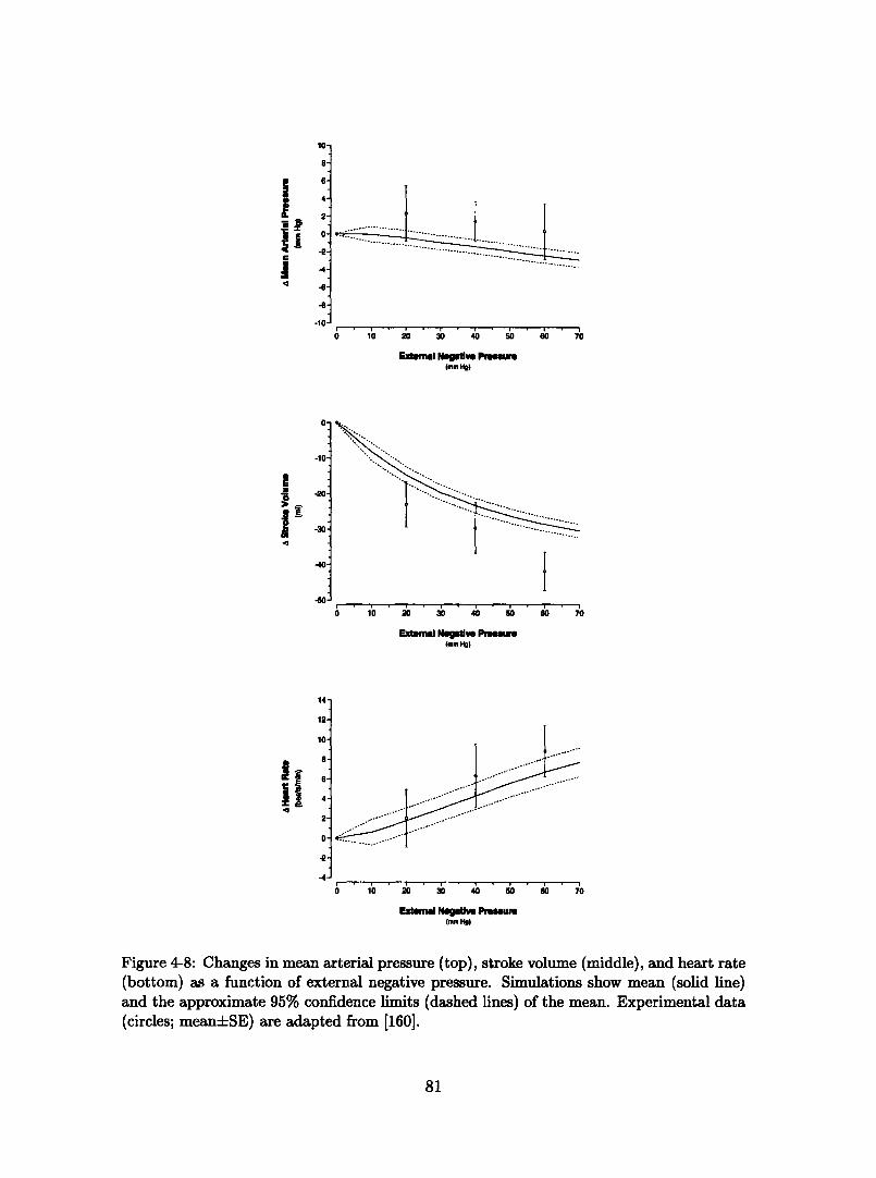
0 10 20 30 40 50 ' 70

Extemma Ngmlve Pmurs(mm Ho)

i0 10 20 30 40 50 60 70

Extal Nqllve Pnomur(mm Hig

0 10 ' ' 30 ' 40 ' 0 0 ' 0 70

Extemal Negatie Pruem(mm HO)

Figure 4-8: Changes in mean arterial pressure (top), stroke volume (middle), and heart rate(bottom) as a function of external negative pressure. Simulations show mean (solid line)and the approximate 95% confidence limits (dashed lines) of the mean. Experimental data(circles; mean+SE) are adapted from [160].

81

aa

I

iiUC

1U.

8.

6'

4.

2'

0-

-2.

-4.

-6.

-8.

.n.

!

I

4

-10

-10.

-240

-,0.

,40

-0

Ii-4II

14'

12

10

a.8'

6'

4.

2'

0.

-2

-4.

-A

-EV

A_

I

arterial baroreceptors become more engaged and the reflex response is mediated byboth cardio-pulmonary and arterial baroreceptors, as evidenced by the significantincrease in heart rate in simulations and experimental data beyond -20 mm Hg of ex-ternal pressure. Both simulations and experimental data suggest a gradual decreasein mean arterial pressure at successively higher levels of LBNP. While the simulatedmean arterial pressure drops below baseline, the experimental data stay above base-line for each level of LBNP. This might again suggest a more powerful compensatoryreflex response in humans as compared to model predictions. However, in this partic-ular experimental study, systolic and diastolic arterial pressures were measured usinga sphygmomanometer with Korotkoff sound detection, and mean arterial pressurewas inferred with the aid of an empirical formula. The differences in the respectivemean arterial pressure responses might very well be within the limits of measurementaccuracy using this technique or might be an artifact of the small number of sub-jects studied. Hisdale [185], for example, reports a drop in mean arterial pressureof 1 mm Hg at the conclusion of a 120 s exposure to -20 mm Hg in twelve subjects.Our simulations predict a drop of approximately 0.5 mm Hg at -20 mm Hg externalpressure.

Despite these discrepancies, the simulated hemodynamic response to lower bodynegative pressure represents the data quite adequately, given that we only matchedthe peripheral resistance response at each level of LBNP.

4.5 Modeling ExerciseFrom a cardiovascular standpoint, exercise manifests itself primarily through a dra-matic increase in cardiac output and blood flow to the exercising muscle groups.Other effects of exercise on the cardiovascular system result from muscular contrac-tions, and include rhythmic muscle-pumping of the leg musculature and an increase inintra-abdominal pressure due to the contraction of abdominal muscles. While changesin breathing pattern might affect intra-thoracic pressure, solid experimental evidencefor this is currently sparse. A direct neural coupling between exercising muscle groupsand the cardiovascular control center in the brain is possible if not likely. However,little is known about afferent pathways and gains of this reflex loop.

In the following paragraphs, we review the experimental evidence that exists foreach of the above mechanisms by which exercise affects cardiovascular function.

Muscle Blood Flow Radegran and Saltin [186] showed that blood flow to anexercising limb increases with a time constant r 10 - 20s. The investigatorsalso demonstrated that the steady-state blood flow to the muscles is linearly relatedto the exercise intensity over the range of 10 to 70 Watts, and that the longer timeconstants correspond to the more intense exercise regimes. They report no immediatechange in the arterio-venous pressure difference at the level of the femoral artery/vein,which implies that the dramatic increase in blood flow can be attributed to a dropin arteriolar resistance of the leg circulation. At higher exercise intensities (100 to145Watts), Pawelczyk and co-workers [187] showed that the leg vascular resistance

82

fails to decrease further, and that changes in blood flow to the legs are mediated byan increase in perfusion pressure.

The lower body compartment in our model is a lumped representation of the legs,the buttocks, and the pelvic circulation. In order to simulate the increase in legblood flow and the decrease in total peripheral resistance seen experimentally duringexercise, we disconnect the arteriolar resistance of the leg compartment from thearterial and cardiopulmonary reflex control and decrease the leg resistance accordingto:

Rll(t) = Rij + (Rf - Rj) · (1 - e-t/7)

where Rjj is the value of the microvascular resistance of the leg compartment imme-diately prior to the onset of exercise; Rf is the final value of the leg vascular resistancefor a given level of exercise intensity, and r is the time constant mentioned above.Rf is determined by matching total peripheral resistance at each level of exerciseintensity to the values seen experimentally.

Muscle Pumps Arnoldi [134] studied the venous pressure in three different loca-tions in the leg circulation, both at rest and during muscular exercise. He showedthat intravascular pressure in the vena tibialis posterior changed in phase with mus-cular contractions. During the contraction phase of the calf muscle, the pressure rose100 mm Hg above the resting level, whereas during muscular relaxation, the venouspressure dropped approximately 50 mm Hg below the resting level. Venous pressuresin two other locations (the vena poplitea and the ena saphena magna) also showedphasic relationships to muscular contractions. However, the pressure excursions fromthe respective baselines were modest in comparison to the ones seen in the vena tibialisposterior.

The action of a muscle pump is simulated by periodically varying the externalbias pressure at the leg compartment. In bicycle ergometry exercise protocols, theangular frequency of cycling is commonly fixed to 1 rev/sec; the exercise intensityis varied through the resistance imposed on the wheels. Thus the sequence of calfmuscle contraction and relaxation is periodic with period 1 s. We represented theexternal pressure at the leg compartment according to:

Pmax' * · (1- cos(4rt)) 0 < t < 1/4Pext -~ Pm, 1/4 < t < 1/2

Pmax 2 (1 + cos(4r(t- 1/2))) 1/2< t < 3/40 3/4 <t < 1

Here Pmax is the maximal external pressure, which depends on the exercise intensity.

Intra-Abdominal Pressure Indirect evidence for a change in intra-abdominalpressure during exercise is given by Williams and Lind [188], who studied esophagealpressures above and below the level of the diaphragm at rest and during static exercise.Their results indicate a modest change in mean intra-abdominal pressure of about5 mm Hg at a moderate exercise level.

83

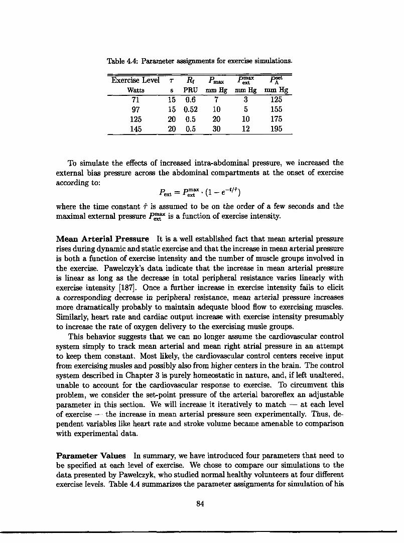
Table 4.4: Parameter assignments for exercise simulations.

Exercise Level r Rf Pm,, P 'ax PAtWatts s PRU mm Hg mmHg mm Hg

71 15 0.6 7 3 12597 15 0.52 10 5 155

125 20 0.5 20 10 175145 20 0.5 30 12 195

To simulate the effects of increased intra-abdominal pressure, we increased theexternal bias pressure across the abdominal compartments at the onset of exerciseaccording to:

Pext = ta (1 - et)

where the time constant f is assumed to be on the order of a few seconds and themaximal external pressure PtX' is a function of exercise intensity.

Mean Arterial Pressure It is a well established fact that mean arterial pressurerises during dynamic and static exercise and that the increase in mean arterial pressureis both a function of exercise intensity and the number of muscle groups involved inthe exercise. Pawelczyk's data indicate that the increase in mean arterial pressureis linear as long as the decrease in total peripheral resistance varies linearly withexercise intensity [187]. Once a further increase in exercise intensity fails to elicita corresponding decrease in peripheral resistance, mean arterial pressure increasesmore dramatically probably to maintain adequate blood flow to exercising muscles.Similarly, heart rate and cardiac output increase with exercise intensity presumablyto increase the rate of oxygen delivery to the exercising musle groups.

This behavior suggests that we can no longer assume the cardiovascular controlsystem simply to track mean arterial and mean right atrial pressure in an attemptto keep them constant. Most likely, the cardiovascular control centers receive inputfrom exercising musles and possibly also from higher centers in the brain. The controlsystem described in Chapter 3 is purely homeostatic in nature, and, if left unaltered,unable to account for the cardiovascular response to exercise. To circumvent thisproblem, we consider the set-point pressure of the arterial baroreflex an adjustableparameter in this section. We will increase it iteratively to match - at each levelof exercise - the increase in mean arterial pressure seen experimentally. Thus, de-pendent variables like heart rate and stroke volume became amenable to comparisonwith experimental data.

Parameter Values In summary, we have introduced four parameters that need tobe specified at each level of exercise. We chose to compare our simulations to thedata presented by Pawelczyk, who studied normal healthy volunteers at four differentexercise levels. Table 4.4 summarizes the parameter assignments for simulation of his

84

exercise protocolThe results in Figure 4-9 show the comparison of our simulations to the experi-

mental data presented by Pawelczyk. We generated the simulation of oxygen uptakeby multiplying cardiac output, CO, by the arterio-mixed venous oxygen difference,Co2(a - D) at each level of exercise, i.e. V0 2 = CO Co2(a - ). We took the valuesof the arterio-mixed venous oxygen difference from Asmussen and Nielsen [189]. Thedashed lines in the oxygen uptake simulation represent a one-a confidence level andare based on the standard error of the arterio-mixed venous oxygen difference.

Over the exercise regime considered in the experimental study, the model capturesquite well the steady-state changes in heart rate, cardiac output, and oxygen uptake.The simulated changes in stroke volume replicate the ones observed experimentallymore qualitatively than quantitatively: an initial increase in stroke volume is followedby decline as the exercise intensity is increased. The faster drop in simulated strokevolume at high exercise intensities might be due to cardiac factors (e.g., inappro-priately low inotropic state) or peripheral factors (e.g., inappropriately low venousreturn).

One should keep in mind, however, that the model was not built with its appli-cation to exercise simulation in mind. Given the relatively simple assumptions madein simulating exercise, the results presented in Figure 4-9 are surprisingly good.

12D

IfIt

1iI

o io - io

PerW"aml

.001 +4i~~~~~~~~~~~~~~

M)~~~r

0 a0 o lio f16

Powe(wQ

10o li0

ji

i 0 4 0 1 0

Poea1

Ioto-

0o

PowP-

Figure 4-9: Changes in heart rate, cardiac output, stroke volume, and oxygen uptake inresponse to sudden-onset exercise. Solid lines: simulations; data represent mean ± SE,adapted from [187].

85

120I 10

..

10

4.6 Summary RemarksIn this first part of this thesis, we have built and validated a computational model ofthe cardiovascular system that is capable of representing the short-term steady-stateand transient hemodynamic response to orthostatic stress.

To achieve this objective, we chose to model the entire hemodynamic systemby a finite set of representative compartments, each of which captures the physicalproperties of a segment of the vascular system. While this approach is incapableof simulating distributed effects, such as pulse wave propagation, it does reproducerealistic values of beat-by-beat hemodynamic variables, and the simulated steady-state responses to head-up tilt and lower body negative pressure agree well withpopulation averaged experimental observations over a wide range of orthostatic stresslevels. In addition, the model is capable of reproducing the transient hemodynamicresponse to sudden gravitational stress quite well.

For now, we are restricted to simulating the early steady-state response of thecardiovascular system to orthostatic stress, since the reflex control model only rep-resents the major neural control mechanisms that are responsible for short term (<5 min) control of blood pressure. Studies have shown that within minutes after theonset of gravitational stress, hormone levels in the circulation rise significantly [36].The addition of hormone loops in the future might allow us to extend the timescaleof our simulations beyond a few minutes.

An inherent limitation to any modeling effort is the degree of uncertainty associ-ated with the numerical values assigned to the various parameters of the model. Wehave tried as much as possible to give a detailed account of the origin of the param-eter values we chose to assign. Where possible, we based nominal parameter valuesand their standard deviations on the results of clinical studies of normal healthy sub-jects. When such data was not available, we supplied physiologically plausible meanvalues, ranges, and standard deviations. This strategy enabled us to estimate errorbounds for our simulation results, which generally agree well with those reported inexperimental studies.

The degree to which the model reproduces steady-state and transient hemody-namic data suggests that the current model architecture includes all the major fea-tures that contribute significantly to the short-term hemodynamic response to or-thostatic stress. Residual discrepancies between simulations and experimental ob-servations are likely due to the particular choices of parameter values and not dueto structural problems in model architecture. Model Optimization should thereforeremedy these residual differences.

Finally, we did not adopt a strategy of minimal modeling. Rather, we built amodel with the aim of representing cardiovascular physiology at a resolution thatallows for simulation of various hypotheses about the mechanisms of orthostatic in-tolerance. The model, in its current state, is therefore highly over-parameterized. Thesensitivity analysis to follow will identify those parameters of the system that con-tribute significantly to a particular output of interest, thus reducing the complexityintroduced by our modeling approach.

86

I

Part II

Sensitivity Analyses andParameter Estimation

87

88

Chapter 5

Sensitivity Analysis

When developing the model presented in the previous chapters, we did not strive tofind a minimal model capable of representing the experimental observations presentedin the previous chapter. Rather, we tried to represent the components of the cardio-vascular system that are commonly thought to play significant roles in orthostaticstress physiology. Consequently, the resultant model is quite complex, representingcardiovascular physiology at a variety of time and space scales.

Increasing the complexity of a model can work against its usefulness in manyrespects: simulation times are increased; parameter values are harder to pick reliably;and it becomes difficult to understand in a fundamental way what parts of the modelare actually being exercised and how. The need to develop tools for model analysisbecomes quite obvious: only if we are able to identify those components of the modelthat contribute significantly to a particular simulated response do we actually increaseour understanding of the system under study; only if we are able to quantify the effectsof parametric uncertainties can we assess the model's range of validity and can wesuggest experiments that might help reduce prediction uncertainties1 . The focus ofthis chapter is therefore on model analysis and, in particular, on sensitivity studiesthat help illuminate the influence individual parameters hold over the variability ofparticular output variables.

We will approach sensitivity analysis from a local perspective, focusing on changesin output variables as the parameters of the model are perturbed about a normaloperating point in parameter space. Questions commonly addressed with such localanalyses involve propagation of errors or finding a direction in input space along whichthe output is maximally influenced, thus establishing a local measure of importanceof parameters or combinations of parameters.

Section 5.1 serves to introduce the terminology and mathematical routines used inthe remainder of this chapter. In Section 5.2, we present the results of the sensitivityanalyses. Rather than performing one sensitivity study, we approach the analysis in

1Uncertainties in mathematical representations of physical or physiological phenomena also arisethrough the assumed mathematical relationships (structure of the model) and the details of theirimplementation on computational platforms. We will not pursue these uncertainties here, but as-sume the model structure and implementation as a framework within which to explore parametricuncertainties.

89

stages. First, we explore the sensitivities of the uncontrolled hemodynamic systemin steady-state. Subsequently, we analyze the controlled cardiovascular system insteady-state, and finally we turn our attention to the steaady-state and transientsensitivities during orthostatic stress simulations. We summarize the conclusions ofthe sensitivity study in Section 5.3.

5.1 Local Sensitivity Analysis

When assessing parametric sensitivities, one is interested in the changes ay inducedin the vector y of model outputs as a result of perturbations aG of the vector 0 ofmodel parameters. Before presenting how ay and ad are related in the framework oflocal sensitivity analysis, we briefly review the nature of the model output y.

The cardiovascular model presented in previous chapters generates values for bloodpressures, blood flows, vascular volumes, cardiac capacitances, and controlled vari-ables, such as heart rate and arterial resistance, with a temporal granularity of theintegration stepsize (on the order of 10- 3 s). Often, one might be interested in theparameters that affect an entire waveform, such as the arterial or central venouspressure waveforms, for example. In such cases, the output vector y consists of thesamples of the waveform of interest, and sensitivities are explored for each sample inthe waveform. If one is interested in analyzing more than one waveform, the modeloutput y can consist of several waveforms, appropriately normalized and stacked ontop of each other. Quite frequently, however, one is not interested in the sensitivitiesof individual samples within a cardiac cycle, but rather in the sensitivities of derivedfeatures of these waveforms and how these sensitivities change under transient condi-tions. Examples of derived features are the mean value, the peak value, or maximumslope of a particular waveform on a beat-by-beat basis. In this case, the output vectory consists of all derived features that are of interest, possibly ordered by beat numberif transient changes in these features are of interest.

In the analysis to follow, we focus our attention on just four derived output vari-ables, namely cycle-averaged arterial pressure, cycle-averaged central venous pres-sure, stroke volume, and heart rate, each of which is defined on a beat-by-beat basis.Focusing on the cycle-averaged changes of just four output variables constitutes asignificant aggregation of the model's output data. However, these four derived vari-ables are the most significant measures of cardiovascular performance, which is thereason for choosing them.

During the first part of the sensitivity analysis, we will be concerned with theparametric sensitivities of just the steady-state values of these output variables. Theoutput vector y in this case simply consists of the steady-state cycle-averaged valuesof the four variables over one steady-state cycle. Towards the end of this chapter, wewill explore the parametric sensitivities of the output variables during the model'stransient response to orthostatic stress simulations. For this, the output vector willconsist of 2400 samples: each variable is sampled at 2 Hz over one minute of supinebaseline and four minutes in the head-up posture. To summarize, the output vectorcan be written as y = [Yl, Y2,..., yn] e 72, where n = 4 for the steady-state analyses

90

__

and n = 2400 for the transient sensitivity study. Similarly, the vector of parametersis given by 0 = [01, 02, . . , 0m] E R7m, where m = 107 is the number of independentparameters of the model.

The effects of parameter changes aGj on changes ayi in a particular output variablecan be expressed in terms of a Taylor series expansion:

a= ayi 1 aAH'yi = 1 m& 'h 0Y22 if 0aj~Ok + " , i = l, ...,n

j=1 li j=l k=l jk

The partial derivatives y1i/0j and 2yi/O8jak are commonly called the first- andsecond-order local sensitivities [190], respectively, while the matrix of the first partialderivatives

J() = () E

is variously referred to as the sensitivity matrix, the Jacobian matrix, or the Fr6chetderivative.

The partial derivative ayi,/l, is an obvious choice for a linear or first-order mea-sure of the local sensitivity of the model output to parameter perturbations, becausefor small enough aj it gives a good approximation to ayi/AOj assuming all otherparameters stay fixed. The second-order derivative 2yi/OGjaOk ascertains the sensi-tivity of the first-order sensitivity aYi/080 with respect to changes in Ok, and thereforeprovide information about the quadratic dependence of the model output on param-eter changes.

As defined above, however, the numeric values of the sensitivity coefficients dependon the units of measurement of both the output variables and the parameters; inorder to compare sensitivities across different input and output variables, the partialderivatives need to be normalized to render them non-dimensional. A commonlyused normalization scheme scales the partial derivatives by the nominal outputs andnominal parameter values:

()j } i=l, ......,n a ij--1 ..... m j=l,.....,m

a s2i i k<62 820 i\aej 8 }=l,...., ... YN ajak ...... nj,k= .... . . . . ..,m ,k---, ... .....,m

to relate fractional changes in output to fractional changes in the parameter values[191].

While efficient methods exist to co-compute accurately the sensitivity matrix alongwith the actual simulation output, these methods are most powerful when the numberof output variables and parameters is small. We rely on a finite-difference approxima-tion to the analytical partial derivatives. Experimentation with the stepsize in a two-sided finite-difference method revealed generally good approximations for stepsizes ofabout 5 % of the nominal parameter values. Owing to the relative efficiency of the

91

associated computations, we routinely compute the first-order sensitivities, Oyi/a0j,and the "pure" second-order sensitivities, 2yi/aOj, for each parameter. Both areO(m) computations for fixed n, where, as above, m is the number of parameters andn is the number of output variables. Assessment of the cross-term second-order sen-sitivities, O2Yi/0jMak (Vj, k; j I k), is computationally substantially more expensive,namely O(m2).

5.2 Results and Discussion

As alluded to in the introductory comments to this chapter, we will perform sensitivitystudies in stages, first examining the parametric sensitivities of the steady-state valuesof the four output variables in the uncontrolled hemodynamic system before repeatingthe analysis for the controlled system. We then turn our attention to the analysis ofthe steady-state response to orthostatic stress, and finally investigate the sensitivitiesof the transient response. Building up the sensitivity studies in such a way allows usto test our understanding of the observed sensitivities at each stage, thus providingmore insight into the results than a single sensitivity study would be able to provide.

In the figures to follow, we display the normalized first-order sensitivities (filled cir-cles) along with the normalized pure second-order sensitivities (open circles), rankedin descending order of the magnitudes of the first-order sensitivities. We also displayseparately the top twenty cross term sensitivities for each analysis, including pureterms if they occur in these top twenty. For each output, we identify by their re-spective parameter indices2 the most important parameters (i.e., highest first-ordersensitivity) or, in the case of cross sensitivities, parameter combinations.

Figure 5-1 shows the first-order and pure second-order sensitivity spectra for thefour output variables when the analysis is applied to the uncontrolled hemodynamicsystem; Figure 5-2 shows the second-order cross-sensitivities. Before commenting onthe importance of particular parameters, several general observations can be madefrom these graphs. First, the spectra of the first-order sensitivity coefficients for meanarterial pressure, central venous pressure, and stroke volume exhibit the same generalstructure: a large number of parameters (70 % - 80 %) have negligible influence onthe output variables as evidenced by the long tail of the distributions at very lowrelative sensitivities; a small number (4 - 10) of parameters hold significant influenceover the output variables and are variably offset from the remainder of parameters; avariable number of parameters constitute an intermediate set gradually joining thesetwo extremes. The structure of the three sensitivity spectra confirms our intuitionthat the model is heavily over-parameterized.

A further observation is that even the largest few of the normalized second-ordersensitivities are only a fraction (one half or less) of the largest first-order sensitivities.In the Taylor series expansion , these second-order sensitivities get multiplied by thesquare of the normalized parameter perturbations (and by the further factor of 1/2).It follows that the contribution of the terms involving the second-order sensitivities

2See Appendix A for the key to parameter indices.

92

-0

CMral Venou Pressure1.0-

TomPM)

1)PI

(41)(47)

(1)iIII3I3it

.-0rCk~ pp".

0 20 40

0.@'

0.'

04-

0.0-

eo de0 10

Parmeter Rnk Paameter Rank

Strol Volume

T1LPe)(7S1("1)

(44)147)

Hwrt Roe1.0D

I

IIJ

0.8'

0,-

OA-

02.

00 00~~~I-fl =C

Paramtr Rank

io 100 0r R20 o nk

Paramete Rank

Figure 5-1: Absolute values of relative parametric sensitivities of the uncontrolled hemo-dynamic model. Solid circles: first-order sensitivities; open circles: "pure" second-ordersensitivities.

will be negligible compared to the terms involving the first-order sensitivities, as longas the normalized parameter perturbations are not larger than 10 - 20 %. It is alsoworth remarking that in general the largest second-order sensitivity seem to involveparameters that are also prominent among those with high first-order sensitivities.

The heart rate sensitivity spectrum does not fit the description just given. In theuncontrolled system, heart rate is a parameter rather than a variable whose valueis determined in part through the action of the reflex system. Being a parameter,heart rate is trivially dependent on its own set-point value which is reflected in thespectrum by a single relative sensitivity of unit value and a corresponding second-order sensitivity that is identically zero.

As indicated in the figure, there is significant overlap among the top parametersof the four output variables: seven parameters suffice to account for the top fiveparameters of all four output variables. These seven parameters are distending bloodvolume (66)3, the arteriolar resistance of the splanchnic vascular bed (53), heart rate

3 Numbers in parentheses indicate parameter indices. See Appendix A for a mapping of parameter

93

1.0-

0.8-

I2IJta

o0-

0.4-

0.2-

0.0

e(41)

M()

(SI,

m~

0 .d~Da-91

1.0-

80 1Q0

0.8-

0.-

OA-

02-i

T(71B1)

0.0-

o 100

IJ I

nflW v. |

Imen AlW Pnure

4 .

, .

Main ArlWa Presure

M.m

(71.71

01. /

o11 711

e . . .. . . ... 4 . . .(e a

Centl Venous Presures.-

i

I15 20

0.8-

0.6-

0J-

0.0-

0 0

0O - 5 ' 10

Palmeter Rank

Srok Volume

0 5 0 R

Peuunaar Rank

T' 109O 71)(41.71)

(S, 71(71.71)(71, eI914. I(41, Oe(47,71)

I

I

Figure 5-2: Absolute values of the second-orderuncontrolled hemodynamic model.

o 5 to 15 Rn

Paamer Rank

relative parametric sensitivities of the

(71), intra-thoracic pressure (31), the venous compliance of the splanchnic vascularbed (34), the ventricular systolic time interval (95), and the right ventricular diastoliccompliance (41).

According to the results presented in Figure 5-1, the principal determinants ofstroke volume are distending blood volume (66), heart rate (71), intra-thoracic pres-sure (31), right ventricular diastolic compliance (41), ventricular systolic time interval(95), venous capacitance of the splanchnic vascular bed (34), and left ventricular dias-tolic compliance (47). To understand these dependencies, we recall that under normalphysiological conditions, stroke volume is determined by the end-diastolic filling ofthe right ventricle. As such, it is dependent on the end-diastolic transmural pres-sure and the end-diastolic ventricular compliance. The latter is a parameter of themodel and features prominently in the hierarchy of sensitivity coefficients. The formerinvolves the luminal right atrial pressure and the intra-thoracic pressure. Thus, intra-thoracic pressure directly affects ventricular filling and therefore stroke volume. Right

94

1.0

II'I

I

0.68

OA

0JS

0.4OA

0.2'

(M "(41. e1(41, 71)(41. M9

ON, 4s)(41, 41),m.

0 5 to

Poaller Rank

O OO o o ,

15 2

I

II

1.0

0.8

0.6

0.42

02,

Hflrt Re1

0.6-

0.-

0.4-

0.0

0 0

e . . . . . . . . . o

0.0-

;5 2D

indices to parameter names.

I ·I · · · · _ · ~~~~~~~~ : . . .

o

hn'EN

--

°eoe

o .ooo

Mean ArterIal Piugeme Central Verne PressureTIrl's)

141) 0.8-

Iat

02-

. ~~~~~~~~~~ .....

Ta)

(s)(1I)

(3(1)

()

_ 0

0 20 '40 0 80 100 0 20 40 0 1 80 100

Pameter Rnk Prmeter Rank

Stroe Volume HIert Rate

TWO(71)(E)(II) 0.8-(411

(61)(Sl)

. 04

%. 0.2

o o k o , 0 _ 00

Top7(1)

(16)141)00)(s

l)

_ C,

0 20 40 80 80 100 0 X 40 0 80 100

Paameter Rank Parameter Rank

Figure 5-3: Absolute values of relative parametric sensitivities of the controlled hemo-dynamic model. Solid circles: first-order sensitivities; open circles: "pure" second-ordersensitivities.

atrial luminal pressure is largely dependent on distending volume (top sensitivity inthe spectrum) and systemic venous compliance. The splanchnic bed has the largestvenous compliance of any vascular bed in our model; its influence on cardiac fillingpressure is therefore largest, which explains its occurrence in the sensitivity spectrum.Finally, ventricular volume is dependent upon the time available for diastolic filling.This is reflected by the heart rate and possibly systolic time interval sensitivities inthe stroke volume spectrum in Figure 5-1. Systolic time interval might also influencestroke volume through the time-varying elastance model as the systolic time intervaldetermines the rate of change of the ventricular elastance and therefore the rate ofchange of ventricular pressure.

Having understood the sensitivities involved in the steady-state analysis of strokevolume, we only need to note that in addition to the parameters that affect stroke vol-ume, the mean arterial pressure spectrum shows the splanchnic arteriolar resistance(53) as an important parameter. In steady-state, mean arterial pressure is determinedto first approximation by cardiac output and total peripheral resistance. Total pe-

95

i0.

0.6-

1 04-I -02-

nn-

1.0-

0.8-

0.6-

0.2-

n Arter Prun Ceal Venous Prsur

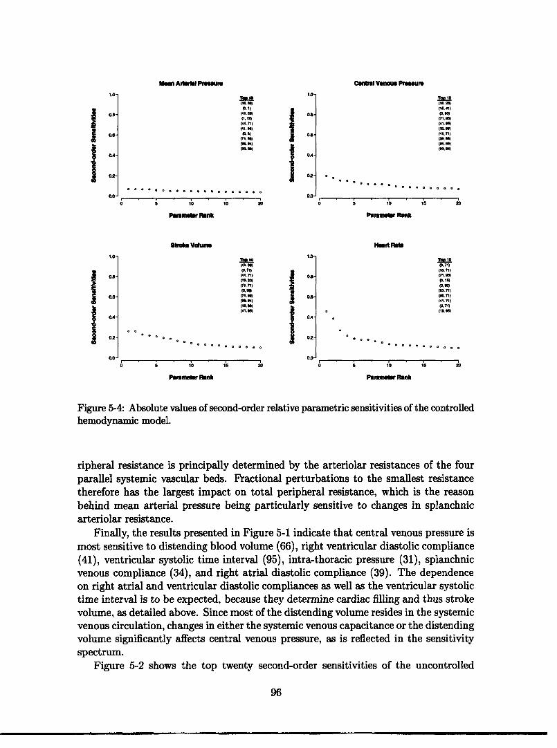
Central Venous Presure

(f. 1)0110.

(41, 711)(41.1

OA-

02

(?l~~~~mO.

ToP 10

(71. ")(41. gm(115 .1(41.711

i- * ° o -·o o o o o . . o o

0 5 10 15 20 0 5 10 15 20

Pnwm'er Rank Pameter Rank

btrom Volume Hrt Re

T A10 (41,co)(% 71)(41.71) 0(It m

(I

* 0

(61.(41. U

02.

0 0 0 I · o o o o · o o o oo 020.0

Tl 10(1 71)

(111(71.11)

(6. 71)(4171)

(IL 66*

0 0 0 . . . . . .

0*5 10 S 20 0 5 10 1s 20

Pamete Rank Paamer RN*

Figure 5-4: Absolute values of second-order relative parametric sensitivities of the controlledhemodynamic model.

ripheral resistance is principally determined by the arteriolar resistances of the fourparallel systemic vascular beds. Fractional perturbations to the smallest resistancetherefore has the largest impact on total peripheral resistance, which is the reasonbehind mean arterial pressure being particularly sensitive to changes in splanchnicarteriolar resistance.

Finally, the results presented in Figure 5-1 indicate that central venous pressure ismost sensitive to distending blood volume (66), right ventricular diastolic compliance(41), ventricular systolic time interval (95), intra-thoracic pressure (31), splanchnicvenous compliance (34), and right atrial diastolic compliance (39). The dependenceon right atrial and ventricular diastolic compliances as well as the ventricular systolictime interval is to be expected, because they determine cardiac filling and thus strokevolume, as detailed above. Since most of the distending volume resides in the systemicvenous circulation, changes in either the systemic venous capacitance or the distendingvolume significantly affects central venous pressure, as is reflected in the sensitivityspectrum.

Figure 5-2 shows the top twenty second-order sensitivities of the uncontrolled

96

j 0.8

04

02

1.0'

0.6

OA-I 0

02

00

Man Ari Pemmu

system. The second-order sensitivities mostly decline gradually rather than exhibitingthe gap structure seen in the first-order spectra. Also, the values of the largest second-order sensitivities for each output variable tend to be smaller in magnitude thanthe corresponding first-order sensitivities. Finally, the top second-order sensitivitiesare almost exclusively comprised of combinations of parameters that also featureprominently high in the first-order sensitivity spectra.

Figure 5-3 shows the sensitivity spectra for the four output variables for the con-trolled cardiovascular system. The general appearance of the sensitivity spectra issimilar to the one of the uncontrolled system in that the output is sensitive only toa small number of parameters. The peak first-order sensitivities generally tend to besmaller than in the uncontrolled system, which can be ascribed to the homeostaticcontrol of mean arterial and mean right atrial pressure: the parameter perturbationsinvariably result in perturbations of mean arterial and mean right atrial pressureswhich lead to reflexive adjustment of effector variables and therefore in reductions ofthe sensitivity values. Generally, the same parameters that rank high in the sensitiv-ity spectra of the uncontrolled system rank high in the corresponding spectra of thecontrolled system. In the controlled cardiovascular system, two additional param-eters, the arterial baroreflex pressure set-point (0) and the cardiopulmonary reflexpressure set-point (15), enter the top group of parameters.

Since heart rate is now a dependent variable rather than a parameter, its sensi-tivity spectrum is non-trivial now, and similar in shape to those of the other threeoutput variables. In addition to depending on its own set-point value, heart rate issensitive to changes in the two reflex set-point pressures and to variables that mostlyaffect stroke volume and arterial blood pressure. Mean arterial pressure becomes acontrolled variable, which is reflected in its strong dependence on its own set-pointpressure and the depression of the remaining parameters in its first- and second-ordersensitivity spectra.

In Figure 5-5, we examine the parametric sensitivities of the four output vari-ables at the conclusion of a three-minute tilt to the 75 head-up position. We chosethis particular time point as it is the recommended reference point for the diagnosisof orthostatic hypotension [29]. The structure of the first-order sensitivity spectraremains almost unchanged from the steady-state analysis of the controlled cardiovas-cular system. Minor changes in the gap structure and in the ranking of individualparameters are apparent. The distance from the carotid sinus to the aortic root (14),the length of the inferior vena cava compartment (96), and the venous complianceof the legs (35) enter the first-order sensitivity spectra due to their importance indetermining the sensed arterial pressure, venous return to the right heart, and theblood volume pooled during orthostatic stress, respectively. The only notable changein the structure of the second-order sensitivity spectra is the isolation of the topthree second-order sensitivity coefficients in the spectrum of the steady-state heartrate response. The spectra of the three other output variables largely stay the same.

The sensitivity coefficients of the cycle-averaged quantities we have been examin-

97

CAmtnl Venous Prur1.0-

ifII

OA-

0.-

0.4-

02-

0.0-

i-iP)P)P)(41)(18)(0)04)(1)(St)

I%.

Pa

0

mwsar Rnk

40 tio

Huit Rea

0.8-

0.6

0.4

02

171)(o)

(m)P.

0 20 40

Par

i oRWrm1r Ronk

so 00o 0 20 40

Figure 5-5: Absolute values of relative parametric sensitivities of the controlled hemody-namic system at the conclusion of gravitational stress. Solid circles: first-order sensitivities;open circles: "pure" second-order sensitivities.

ing will evolve from beat to beat if the system is undergoing a transient, rather thanbeing in (cyclic) steady state, for instance during simulations of orthostatic stresstests. Figures 5-1 through 5-6 therefore represent just one snapshot of the contin-uously evolving sensitivity coefficients. In Figure 5-7, we show the ranges of theabsolute values of the beat-to-beat first-order sensitivity coefficients over the entireperiod of the three-minute tilt to 75°, including a two-minute supine baseline period.The ordering of the parameters is the same as in Figure 5-5.

The general shape of the sensitivity spectra in Figure 5-7 is quite comparable tothe ones discussed in previous figures. However, the numerical values of the sensitivitycoefficients, and therefore the relative importance of particular parameters, dependquite strongly on when the sensitivities are computed, as indicated by rather largenumeric ranges observed for some parameters.

98

II

Ia

a14)M)(14)is)PS)

0.8

0.

OA

02

0.0

0 20 40 R0nk

Pam mf Ronk

o ti0

8balM VolumN

fV

Jiit

0.8

0.6

02

T"4

Ps)

PI

itUI

I

Pa

nk

mets Rink

0 10

| lI

1�11111�11.· · · · ·- ;

WMn Aw 1MM.A1,0

:

I.

Ir

.A1.' . _

1.

I

I..'·- cI.%~bb~6b

n,v~

ngU-

Cnatrl Venmo Prnimure

To 0(71. 4

(IL 14)(0.71)

M.(71.71)

(l5La=

1.0-

I

io O. 0 Q O O O O O O

0.8-

0.6-

0.4-

02-

0.0-

0 5 tO 15 20

Pmtu r Rank

Too to(7. 7)(71. 0

(al )(10.2l)

(15.41)(41.71)(116l

(41,.-

o

0000 .o o o o

oo o

0 Ri5 k

Prmioetr Rank

Stroie Volume

15 20

Heart Rte1.-

I

iIiI

0.8-

.0-

0.4-

0.2-

0.0-

To 10

(0.71)(71.71)

(Iw

(15. 1)

(71.4)(t6.71)

5.0-

iII2

°o000o

00°00o0ooo

0 5 10

Parameter nk

0-0.

0.0-

0.4-

0.2-

0.0-

I5 20

Figure 5-6: Absolute values of second-ordersion of gravitational stress.

Too 10(o, 71)

(1. 71)

(0, 15)(0.56)

(0.)

(3M 71)M&5.Be

0 0 0 0 0 0 0 0 0° o 0 0

60 5 0

nParmer Rank

I5 20

relative parametric sensitivities at the conclu-

5.3 Summary and Conclusions

In the previous section, we have investigated the local first- and second-order sen-sitivities of four output variables to the 107 parameters of the model. While wehave focused our attention on ranking the parameters from very important to non-influential on the basis of the magnitudes of their first-order sensitivity coefficients,we have to keep in mind that the analysis presented is truly local, in the sense that itis only valid in the neighborhood of the local operating point. Furthermore, we haveseen that during transient simulations, the sensitivity spectra depend quite stronglyon time. The notion of a parameter hierarchy therefore becomes a function of timeand operating point rather than being a universal concept. However, several generalconclusions can still be drawn from the results presented in the previous section.

As elaborated on in the previous section, the normalized first-order sensitivityspectra all exhibit a similar structure: a long tail at very low relative sensitivities, asmall number of parameters at high relative sensitivities, and an intermediate zoneof variable length joining the two extremes. For the steady-state analyses shown

99

1.0,

IiJIIiJ

0.8-

0.6-

0.4-

0.2-

0.0-

. . . . . . . . . . . . . . . . .

Lin Arlbl Polure

o

o o

Cltenl VenoUs PureI.O.

II

II ,II11IIII Illll111 Illl111lll1111111111111 l1111111.hl.1 1 . @ . -..... 1 , .. 11ll.,...

PamMiIn Rnk

0.-.

0.e-

0.4-

02-

0o.6o 100

8tae Volume1.0-

I

IIIli 11i1 ii ldlill i,,1,1,,,,,,,,,,,,,, .... l~~~I , I, ,.,1 1 .... I

2 Pmm 4 r0 e

Parroar Ronk

0.0-

0.-

0.4-

02-

0.0-6so o

PmnMrt Rnk

Hlart Rlb

~~~~~~~~~~~~~i I,.. 0 ) P e R k 40 o

Palrme r Rank

Figure 5-7: Ranges of the relative parametric sensitivities of the controlled hemodynamicsystem during gravitational stress. Ordering of parameters is the same as in Figure 5-5.

in Figures 5-1 - 5-5, approximately 70 - 80 % of parameters can be labeled non-influential while only about 5 % of the parameters have significant impact on thesteady-state values of the four output variables. The second-order sensitivities aresufficiently small that their effect is negligible for normalized parameter variations ofup to 10 - 20 %.

Several parameters rank consistently high in the sensitivity analysis and are vari-ably offset from the remainder in the first-order sensitivity spectra. These are thearterial baroreflex set-point pressure (0), the cardio-pulmonary set-point pressure(15), distending blood volume (66), and the heart rate set-point (71). The ventricu-lar systolic timing parameter (95) and the right ventricular diastolic compliance (41)complement the list of top-ranking parameters for stroke volume and central venouspressure.

The arterial baroreflex and the cardio-pulmonary reflex set-point pressures de-termine the steady-state values of mean arterial and mean right atrial pressure, re-spectively. However, they also affect the transient response to gravitational stressthrough their influence on the effector variables. In the absence of homeostatic blood

100

1.o-

0.8-

0.-

OA-

02-

iII{

0.0-I...iI..I..11,.i.... ..

' 100

1o-1.0-

I .

02-

00-,,I, ,1.1,

O0 100

11 11111 ....11'1 111lllllllll111

Mm Arlrl eu

I

I... IJ ,

pressure control, the heart rate set-point determines heart rate completely. In thepresence of neural control, it only partially determines heart rate, as reflex fluctua-tions contribute to the instantaneous heart rate signal. Nevertheless, the heart rateset-point remains an important determinant of the instantaneous heart rate signal.It also affects, along with the systolic ventricular timing parameter, the time periodfor cardiac filling, thus affecting central venous pressure and stroke volume. Finally,distending volume is universally important to all four output variables.

Several other parameters enter the hierarchy of top parameters, depending on theintervention being simulated, on when in the intervention the analysis is performed,and where in parameter space the model is being exercised.

101

102

Chapter 6

Parameter Estimation

Our modeling strategy has focused on building a computational model based on ourunderstanding of the cardiovascular system. More specifically, in Chapters 2 and 3 wedeveloped the model based on analysis of the physical and dynamic properties of thevarious segments of the vasculature and the reflex system. The resultant model hasrelatively high spatial and temporal resolution for its ultimate application, involvesa large number of parameters, and exhibits rich dynamic behavior spanning severaltime scales. Such an approach, in which a model is built from detailed analysis of theunderlying physical processes, is commonly referred to as forward modeling.

In this chapter, we will change perspective and use data in conjunction with ourmodel to estimate the values of some of the model parameters. Such a strategyfalls under the general umbrella of inverse methods in which attributes of a sys-tem are estimated based on measurements that are only indirectly related to theseattributes [192]. In parameter estimation problems, the parameters of a model aretuned such that a measure of error between the model output and a corresponding setof observations is minimized. Methods for solving this minimization problem dependquite naturally on the error criterion and on the structure of the model. Furthermore,the quality of the resultant parameter estimates also depends on the fidelity of theavailable data.

The signals available from physiological experiments are usually very few in num-ber. Quite often, the only signals recorded are beat-to-beat mean arterial pressureand heart rate. Thus a disparity exists between the high resolution and rich dynamicbehavior of the model and the low resolution and limited dynamic behavior of themeasurements. In Chapter 5, we have already encountered one aspect of this mis-match between high detail of the model and low richness of cycle-averaged data: thefour output variables of the sensitivity analysis were insensitive to perturbations in alarge number of model parameters. In the parameter estimation setting, this dispar-ity leads to a very sensitive, or ill-conditioned, estimation problem. Any parameterestimation scheme in this setting needs to address this ill-conditioning.

In Section 6.1, we discuss the error criterion and the method of solving the min-imization problem. In particular, we will discuss the method of subset selection toovercome ill-conditioning of the estimation problem. In Section 6.2, we present theresults of the parameter estimation algorithm when applied to the transient hemo-

103

dynamic response to head-up tilt. We conclude in Section 6.3 by summarizing theresults.

6.1 Non-linear Least Squares and Subset Selection

If the model outputs are linear functions of the model parameters, and if the errormeasure is chosen to be the sum of squares of the prediction error on each output, theresultant minimization problem is the well-known linear least squares problem. If themodel output is a non-linear function of the parameters, the minimization problemis usually solved iteratively through a sequence of linear least squares problems thatinvolve the gradient or higher-order derivatives of the cost function.

Below, we first discuss a particular iterative scheme, known as the Gauss-Newtonmethod. We subsequently point out the manifestation of ill-conditioning in termsof the condition number of the Hessian matrix H, and describe the subset selectionalgorithm that aims to overcome this ill-conditioning. We conclude by giving imple-mentational details and describing the formulation of the estimation experiments, theresults of which will be presented in the next section.

6.1.1 Non-linear Least Squares Estimation

Let 4(k(G),y) denote a non-negative measure of error, or cost function, betweenmodel output k(G) E Rn and experimental data y E Rn. Through the model output,E is an implicit function of the vector of model parameters 0 E R and can thereforebe considered a function from Rm to the non-negative real line, = 4(0) : Rm o

R+ U {0}, for a given experimental data set. Since we aim to minimize this measureof error iteratively, we seek a computational scheme that provides us with a newparameter vector 01 such that (1) < (0o) given an initial best guess 0 0. Oncesuch a A has been identified, it can assume the role of 00, and we can repeat thecomputational scheme in an effort to reduce the measure of error even further.

Let us assume that a second-order Taylor series approximation i of 4(O) is agood approximation of the local behavior of the cost function for small perturbationsAG = 0 - 00 around the initial parameter estimate. [(G) is the best second-orderapproximation to the surface defined by 4(G) around 0o.] TI(0G) is given by

CO) = o) + [D] AO 2 A[a 2 ] AO(o)=cI(oo)+jj oo+IeT L2o G2 00o

where [/a0]o. and [02O/a02]0 are the appropriate matrices of the first- andsecond-order derivatives evaluated at the current best guess of the parameter vectoras indicated by the subscript 0 0. To find its minimum, we equate to zero the gradientof ():

a. F( A+G =000 0 002 ,]

104

__

which leads to the following condition for the stationary point 01:

2 ( 8 1 -° ) = -0 70

If the inverse of the second-order derivative matrix exists, the stationary point isgiven by:

[1= 0 ] - 1 [0] (6.1)

It can be shown that 4D(01) < (G0o) if and only if the matrix of second-order deriva-tives is positive definite [193, p. 86].

Note that we have not yet specified the cost function . The results obtained sofar only require it to be twice differentiable. Let us assume now that we are aimingto minimize the square of the residual error r(O) = t(O) - y between model outputand actual measurements, that is

1 12 1 1O(0) = Ir(*)11 2 = 1.II() - yll2 = * rTr -+ min2 2 2

where the factor of 1/2 has been included for convenience, and the superscript T

denotes transposition. The gradient of this cost function is given by:

[9 =JT r(O) where Jij= ari() a-i(O)

J E RI Xm denotes the Jacobian matrix of the error vector with respect to the param-eter vector. Similarly, we can compute the elements of the Hessian matrix H E Rm X mof second derivatives of the cost function:

0H0 = (JT J), + Z rL a. aj (6.2)" iHij = O j 1=1 i

Note that for small residuals, the Hessian can be approximated by

1Hij3= oo, (JT J)i (6.3)aejoia

since the second term involves the elements of the vector of residuals directly. Thisapproximation is known as the Gauss-Newton approximation to the Hessian.

Inserting the expressions for the derivatives into Equation 6.1, we obtain theiterative parameter updates of the Newton method:

H (i+l - i) = _JT r (6.4)

and the Gauss-Newton approximation thereof:

JTJ (Oi+l - oi) = -J* r (6.5)

105

Let R denote either the full Hessian H or its Gauss-Newton approximation JTJ.If R has full column rank, Equations 6.4 and 6.5 can be solved exactly or in a leastsquares sense, depending on whether or not JT r is in the column space of R. Ineither case, however, the solution is unique, and efficient algorithms exist to solvethe set of linear equations numerically [see, e.g., 194, Chapter 5]. If, on the otherhand, R is rank-deficient, then the m columns of R actually contain less than mlinearly independent vectors. As a consequence, R is semi-definite with at leastone of its eigenvalues at zero. The following argument by Burth and co-workers [195]illustrates the problem of a singular matrix R in the context of parameter estimation.Assume R has a single eigenvalue at zero with some associated eigenvector . Withinthe limits of our second-order approximation, 09 can be added to any step directionwithout affecting the error criterion, since

R -(+i+1- Oi + ) = R (i+ 1- i) ± R. 9 = R (0i+1- 0i) = -JT r

This implies that we can arbitrarily change parameter values along the directionof t9 without affecting the error criterion. Such indeterminacy suggests that theparameters of the model cannot be estimated uniquely from the given measurements;the estimation problem is said to be ill-conditioned.

Frequently, the matrix R is not exactly rank deficient but quite nearly so, inthe sense that the largest eigenvalue is orders of magnitude larger than the smallesteigenvalue. Closeness to singularity is measured by the condition number K(R) which,for real, symmetric matrices, is given by the ratio of the largest to the smallesteigenvalue.

Burth reviews several related consequences of a large condition number for esti-mation problems [195]. We simply note here that a hallmark of an ill-conditionedproblem is its extreme sensitivity to small perturbations in either the experimentaldata or the elements of the matrix R. In the following section, we discuss subsetselection as an approach to overcome this ill-conditioning.

6.1.2 Subset Selection

Subset selection aims to determine which parameter axes lie closest to the singulardirections of the Hessian matrix [196]. Changes in the corresponding parametersdo relatively little to change the fit of the model to the data, and therefore theseparameters are hard to estimate reliably. Once these ill-conditioned parameter axesare identified, one can fix the associated parameters at prior values throughout theestimation process, thus improving the conditioning of the resultant reduced-orderestimation problem. Fixing values of the ill-conditioned parameters has the effect ofintroducing some bias error into the model, but by removing these parameters fromthe estimated set, we improve the reliability with which the remaining parametersare estimated.

Subset selection is most powerful if the eigenvalue spectrum of the Hessian matrixexhibits a large gap between p large eigenvalues and m - p small ones. Such asituation suggests that the Hessian matrix has numerical rank p and that m - p

106

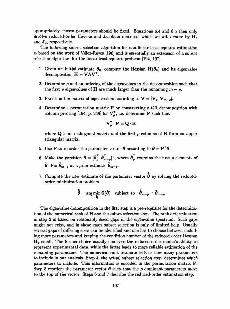
appropriately chosen parameters should be fixed. Equations 6.4 and 6.5 then onlyinvolve reduced-order Hessian and Jacobian matrices, which we will denote by Hpand Jp, respectively.

The following subset selection algorithm for non-linear least squares estimationis based on the work of Velez-Reyes [196] and is essentially an extension of a subsetselection algorithm for the linear least squares problem [194, 197].

1. Given an initial estimate o0, compute the Hessian H(o 0) and its eigenvaluedecomposition H = VAVT .

2. Determine p and an ordering of the eigenvalues in the decomposition such thatthe first p eigenvalues of H are much larger than the remaining m - p.

3. Partition the matrix of eigenvectors according to V = [Vp Vm_p].

4. Determine a permutation matrix P by constructing a QR decomposition withcolumn pivoting [194, p. 248] for VPT, i.e. determine P such that

Vp P=Q-R

where Q is an orthogonal matrix and the first p columns of R form an uppertriangular matrix.

5. Use P to re-order the parameter vector 0 according to 0 = PT.

6. Make the partition B = [bT _p]T, where 0p contains the first p elements of

6. Fix Om-p at a prior estimate Om-p.

7. Compute the new estimate of the parameter vector 0 by solving the reduced-order minimization problem

0 = arg min (0) subject to Om-p = Om-p

The eigenvalue decomposition in the first step is a pre-requisite for the determina-tion of the numerical rank of H and the subset selection step. The rank determinationin step 2 is based on reasonably sized gaps in the eigenvalue spectrum. Such gapsmight not exist, and in those cases subset selection is only of limited help. Usuallyseveral gaps of differing sizes can be identified and one has to choose between includ-ing more parameters and keeping the condition number of the reduced order HessianHp small. The former choice usually increases the reduced-order model's ability torepresent experimental data, while the latter leads to more reliable estimation of theremaining parameters. The numerical rank estimate tells us how many parametersto include in our analysis. Step 4, the actual subset selection step, determines whichparameters to include. This information is encoded in the permutation matrix P.Step 5 reorders the parameter vector 0 such that the p dominant parameters moveto the top of the vector. Steps 6 and 7 describe the reduced-order estimation step.

107

6.1.3 Numerical Implementation

The computations of the Jacobian and Hessian matrices have been described in Sec-tion 5.1.

There are three major computational steps associated with the subset selectionalgorithm outlined above: the eigenvalue decomposition of the Hessian matrix; theQR-decomposition with column pivoting of the matrix of eigenvectors; and the least-squares estimation of the reduced-order problem.

To solve the eigenvalue problem, we were guided by Algorithms 8.3.1 - 8.3.3 fromGolub and van Loan [194, p. 415-421]. We start by converting the real, symmetricHessian matrix H to a symmetric tridiagonal matrix through a sequence of similaritytransformations based on Householder reflections [198]. Subsequently, the lower right-hand tridiagonal 2-by-2 submatrix is diagonalized iteratively through a sequence ofimplicit, symmetric QR steps with Wilkinson shifts using Givens rotations [199]. Thisstep is repeated on the next trailing lower right-hand tridiagonal 2-by-2 submatrixuntil the entire tridiagonal matrix is diagonalized. The resultant matrix carries theeigenvalues of the Hessian along the diagonal. By accumulating the sequence ofsimilarity transformations, we assemble the matrix of eigenvectors. Finally, we applypermutation matrices to reorder the columns of the eigenvalue and the eigenvectormatrices such that the diagonal matrix contains the eigenvalues in descending orderof their magnitudes.

We implemented the QR-decomposition of the eigenvector matrix V accordingto Businger and Golub [200]. The algorithm applies a sequence of Householder re-flections to the columns of V so that the lower diagonal portion of each column issuccessively set to zero. At each step of this reduction to upper triangular form, thealgorithm chooses the column with the largest sum of squares to be reduced next,thus implementing the column pivoting strategy. The same QR-decomposition is atthe core of the algorithm for solving the reduced-order least-squares problem. Thealgorithm consists of a QR-decomposition of the reduced Jacobian matrix, the appli-cation of the transposed orthogonal matrix QT to the vector of residuals, and solutionof the resultant set of equations through backsubsitution. Finally, we use an iterativerefinement scheme to improve the estimate of the solution vector.

We implemented the subset selection algorithm in the C programming languageand extended the program to run on a five nodes, ten processors, Linux-based parallelcomputational platform using the message-passing interface.

6.1.4 Formulation of the Estimation ProblemIn the following section, we apply the subset selection algorithm to the problem ofestimating parameter values from the transient hemodynamic response of transitionsfrom supine to the upright posture. In keeping with the analysis of the previouschapter, the vector of output variables consists of cycle-averaged arterial pressure,cycle-averaged central venous pressure, stroke volume, and heart rate. Each variableis computed on a beat-by-beat basis, linearly interpolated between beats, and re-sampled at 2 Hz. We include one minute of supine baseline data and four minutes in

108

the upright posture leading to an output vector k(0) that contains 2400 samples. Wenormalize this output vector by the samples of the data vector y, so the elements ofthe output vector are unitless. Thus, we aim to minimize the relative error betweensimulation output and measurements:

1 i() -Yi4(0) = - iTi where ri = Yi)-2 i

We similarly normalize the columns of the Jacobian matrix by the elements of thetarget vector.

In this chapter, we are interested in evaluating the performance of the subsetselection algorithm as applied to our computational model. In order to do so, weneed to know the true parameter values underlying the experimental data that thealgorithm is supposed to match. We therefore use the cardiovascular model in aforward sense to generate synthetic "measurements" that serve as the target for theestimation routine.

We will approach the evaluation in two stages. In the first stage, we will fix theill-conditioned parameters at their "true" values; the only parameter values that differbetween 80 and the target "measurements" are the well-conditioned parameters. Thisapproach allows us to assess the quality of the resultant parameter estimates in theabsence of possible influences from the ill-conditioned parameters. In the second stage,we vary all parameters to generate the target data. More precisely, we generate the"measurements" by randomly perturbing the parameter vector 0 around its nominalvalue 80 using a Gaussian density with mean 80 and standard deviation of 10 % ofeach parameter's nominal value. In both stages, we generated the target vector bysimulating the transient response to a 750 degree head-up tilt using the perturbedparameter vector. We subsequently reset the parameter vector to 80 in order to startthe estimation procedure.

To assess the estimation algorithm's sensitivity to noise in the target data, weadded to the target vector zero-mean Gaussian white noise with a standard deviationof 2.5 % of each target sample.

Finally, we will exclusively work with the Gauss-Newton approximation of theHessian matrix since it is computationally much less expensive to compute than thefull Hessian.

6.2 ResultsFigure 6-1 shows the eigenvalue spectrum {Ai} of the approximate Hessian matrixH(0o) = JTJ. Since the spectrum covers almost eight orders of magnitude, we plotthe eigenvalues on a logarithmic scale. The corresponding condition number of thefull-order Hessian matrix is K(H) = 3.4. 107, indicating substantial ill-conditioning ifattempts were made to solve the full-order estimation problem. Figure 6-2 shows thegap structure {Ai/Ai+l } of the eigenvalue spectrum. It is evident from the two figuresthat no single dominantly large gap exists that would suggest an obvious choice for therank estimate. However, Figure 6-2 does show three breakpoints that are sufficiently

109

10'-

1CUf -10 -

10J

To 1042001

10.42.42

;6 4.0

% s. 1. o 3

(_ 2

4.74.53.72.42.2

06 20 ~ eo eo 1oo 0 20 40 s o so 1

Index I Ide I

Figure 6-1: Eigenvalue spectrum of the Hes- Figure 6-2: Gaps Ai/Ai+l of the eigenvaluesian matrix. spectrum.

removed from the remainder of the spectrum. They correspond to the rank estimatesP = 3, p2 = 1, and p3 = 4, where pi corresponds to the largest gap, p2 to the secondlargerst and so on. We will explore each of these rank estimates along with a fourthone, p = 15, to demonstrate the effect ill-conditioning can have on the parameterestimates.

In the first stage of our analysis, we are interested in whether the optimizationalgorithm can recover the well-conditioned parameters when the ill-conditioned pa-rameters are fixed at their "true" values. The results of this analysis are shown inFigures 6-3 and 6-4. For each parameter included in the optimization, we display therelative error between the parameter's starting value and its true target value by ablue diamond. The red solid circles indicate the relative error between the final pa-rameter estimate and the parameter's true value. Parameter estimates were accepted,once the cost function i(O) met the preset termination criterion, (9) < y, where yis an appropriately small constant. Each result is based on ten runs of the estimationalgorithm for different noise realizations of the target vector.

The results in Figure 6-3 demonstrate that in each of the reduced-order estimationproblems, the algorithm returns parameter estimates that are very close to, if notindistinguishable from, their true values (mean relative error of zero), despite initialrelative errors of up to 26 %. In fact, the residual bias in some of the parameterestimates can be reduced even further by using a more stringent termination criterion.The parameters identified are the arterial baroreflex pressure set-point (0), the rightventricular end-diastolic compliance (45), distending blood volume (70), and the heartrate set-point (90)'.

Figure 6-3 also demonstrates that the reduced-order parameter estimates are ex-traordinarily insensitive to perturbations of the target "measurements". In fact, for

'Numbers in parentheses indicate parameter indices. See Appendix A for a mapping of parameterindices to parameter names.

110

.1

I · · · I I 1-

Table 6.1: Mean relative errors of estimated parameters with respect to their true values.Numeric values are given in %.

Parameter Indices

K(Hp) 0 45 70 90

p-= 4 55.3 (-0.9±0.3) (0.1±0.2) (0.4±0.1) (0.7±0.4)

p=15 8.0. 104 (-21.1±2.5) (4.6±4.2) (-5.6±1.2) (32.1±6.8)

each parameter estimate shown in the figure, there are ten red circles correspondingto the ten runs of the algorithm for different noise realizations. For most estimates,it is impossible to resolve visually more then two of these red circles.

This situation changes dramatically, however, if we attempt to identify ill-condi-tioned parameters. The results of such an attempt are shown in Figure 6-4, wherewe included 15 parameters in the analysis. The results demonstrate that inclusion ofill-conditioned parameters leads to failure to converge to the true parameter values(large bias) and severe sensitivity of the parameter estimates to perturbations of thetarget "measurements" (large variances of the parameter estimates). Mean relativeerrors between the parameter estimates and the true target parameter values are ashigh as 450% with standard deviations as high as 180%. In Table 6.1, we sum-marize the results of the well-conditioned estimation problem shown in the bottompanel of Figure 6-3 along with the estimates of the same parameters as derived fromthe ill-conditioned problem of Figure 6-4. A large condition number of the Hessiancorresponds to large mean relative errors and comparatively larger variances.

We want to emphasize that the parameter estimation runs shown in Figure 6-3and 6-4 used the same termination criterion. This implies that no assessment of thequality of the parameter estimates can be based on the residual error or its norm.

In any realistic situation, we cannot assume that the ill-conditioned parametersremain at their "true" values. This issue is addressed in the second stage of ouranalysis, where we allow all parameters to vary from their respective nominal valueswhen generating the target response. The ill-conditioned parameters are subsequentlyset to their nominal values for the estimation algorithm, and only the well-conditionedparameters are estimated. The results of this second stage are shown in Figures 6-5and 6-6.

In Figure 6-5, we show the results of the well-conditioned problem. As in Fig-ure 6-3, the parameter estimates are quite close to the true target parameter values.Furthermore, the parameter estimates are again extraordinarily insensitive to pertur-bations of the target "measurements". However, as compared with the correspondingresults shown in Figure 6-3, the bias of the some parameter estimates is larger, becausethese estimates attempt to compensate for the incorrect (nominal) values assumed forthe ill-conditioned parameters. Despite the gentle increase in bias in some estimates,the estimation results of the well-conditioned problem is still good, with a maximumrelative error of approximately 3 %.

111

p =1

1:70

1 2 3 4 5 e 7 8 9 1O 11 12 13 14 15

Pamete Rank

p =3

Key1:0

2.703:90

* .

4 5 e 1 12 13 14 nk

p=4ara er nk

p =4

1:02903:454:70

1 2 3 4 5 i 7 6 ' 1O 1 1 2 13 14 15

Parameter Rank

Figure 6-3: Relative errors between initial parameter values and target values (blue dia-monds) and final parameter estimates and target values (red circles) for three rank estimates.Ill-conditioned parameters kept at their "true" values. They key in each figure relates theparameter rank to the respective parameter index.

112

02-

0.1 -I

I0.0-

4.1-

0.3-

02-

0.1 -

I

0.2-

0.3-

02-

0.1 -

I19

-02-

-0.3-

--------- ----------------------------------------------

0

0.1 -

Figure 6-6 displays the results of the parameter estimation if ill-conditioned pa-rameters are once more included in the analysis. The results are as unstable as theones presented in Figure 6-4.

6.3 Summary and ConclusionsThis chapter focused on estimating parameters of the cardiovascular model from "ex-perimental" data. In particular, we employed a non-linear least squares optimizationroutine with subset selection. The latter was necessary to overcome the severe ill-conditioning of the estimation problem.

The results presented are quite promising in that the parameter estimates derivedfrom solving reduced-order problems are quite well-conditioned and have little biaseven if the ill-conditioned parameters are allowed to vary.

We consider the work presented in this chapter the beginning of our effort to esti-mate parameters from experimental data. Future work needs to analyze the qualityof the parameter estimates in relation to the number of signals included in the anal-ysis. We did not address the issue of row and column scaling of the Hessian matrix,but simply remark here that subset selection results are not scaling-invariant. Onecould potentially exploit such a fact to improve the estimates of parameters that arecurrently ill-conditioned.

p =15

0.2-

0.1-

I 0.0-

-02-

A '%.

* .

. .* - * * *

.--- +---.....--------... --.-- .........-----.--- . : · I

: '. I·I

· 8

1 2 3 4 5 6 7 8 9 10 11 12 13 14 15

Parmlner Rank

Figure 6-4: Relative errors between initial parameter values and target values (blue dia-monds) and final parameter estimates and target values (red circles). p = 15. Ill-conditionedparameters kept at their "true" values.

113

p=1

1:70

.......................................................................

1 2 3 4 6 7 8 9 10 11 12 13 14 15

Paramm Rank

p =3

1:02:703:46

..-------. .. ...... ....................................................* 0

1 2 3 4 5 0 7 8 90l 11 12 3 14 s

Parameter Rank

p =4

1:0:00

3:453:70

...................................I

v

1 2 3 4 P 6 7 8 9 10 nm 12 13 14 nk

Parameter Rank

Figure 6-5: Relative errors between initial parameter values and target values (blue dia-monds) and final parameter estimates and target values (red circles) for three rank estimates.Ill-conditioned parameters not kept at their "true" values. They key in each figure relatesthe parameter rank to the respective parameter index.

114

02-

I

I

0.1-

0.0-

-0.1-

-0.2-

-0.3-

0.2-

0.1-

0.0-

-0.1-

I

IIC

-02-

-0.3-

03-

02-

0.1-

0.0-

-0.1-

Ii

02-

-0.3-

v

p =15

U.3

0.2

0.1

an'l al

0.2-

,4.3

* . *;, ! * sI *9 . I

I

1 2 3 4 5 6 7 10 i2 1 9 14 15

Parameter Rank

Figure 6-6: Relative errors between initial parameter values and target values (blue dia-monds) and final parameter estimates and target values (red circles). p = 15. Ill-conditionedparameters not kept at their "true" values.

115

^^

116

Part III

Clinical Study and Model-basedData Analysis

117

118

Chapter 7

Clinical Study

The transient cardiovascular response to changes in posture has been under investi-gation by various groups of researchers over the past three decades. Of particularinterest has been the question of whether active standing and passive tilting elicit thesame sequence of hemodynamic events.

In a series of publications, Rossberg and co-workers [201-203] investigated thetransient heart rate response to rapid head-up tilt. They report that rapid tilt to 70°

(over 1.5-2 s) elicits a strong reflexive increase in heart rate, comparable in magnitudeand timing to the ones observed during active standing [204]. Borst and co-workershad previously hypothesized that the initial heart rate response to active standing wasat least in part due to a central command-mediated muscular exercise reflex [204].This mechanism would clearly be absent during passive tilt and, therefore, wouldnot explain the purported similarity of the two responses. Subsequent studies of theheart rate response to active and passive changes in posture failed to reproduce thedramatic responses reported by Rossberg [136, 205-207].

Similarly, several investigators have focused on the arterial blood pressure responseto active and passive changes in posture [135, 136, 206-208]. The data presentedby Sprangers and co-workers suggest no significant [206] or only a modest drop inarterial blood pressure for a very brief period of time ( 5s) in response to rapidtilts [136, 207]. The data presented by Tanaka and colleagues [135] suggest, however,that the timing of arterial blood pressure drop and heart rate response are intimatelylinked and are approximately the same for active and rapid passive changes in posture.Consistent with Sprangers' findings, Tanaka reports a smaller increase in heart rateand a smaller drop in mean arterial pressure for rapid tilts than for standing up.

To understand better the transient hemodynamic events during active and passivechanges in posture, and in the of hope resolving some of the discrepancies betweenvarious reports in the literature, we designed a clinical study that aimed at elucidatingthe hemodynamic response during the first 180 s after the onset of orthostatic stress.In particular, we were interested in identifying the continuous transient response ofarterial blood pressure and heart rate to active standing, rapid tilting, and slow tilting.

119

7.1 MethodsSubjects We recruited ten healthy volunteers (five males, five females) to partic-ipate in this study. The mean age was (28.7±1.2) years, the mean body height was(172.8±4.0) cm, and the mean body weight was (70.6±4.5) kg (see Table 7.1 for in-dividual subject information)l. Participants regularly engaged in light to moderatephysical activity (none was a performance athlete) and had no sign of cardiovasculardisease.

Table 7.1: Subject information.

Subject ID Gender Age Height Weightyears cm kg

12726 M 28 170 6412734 M 30 165 6412744 M 28 180 10012754 F 26 160 6112755 M 32 192 8312814 F 27 165 5612815 F 22 185 7312819 F 28 155 5512821 F 32 173 7713960 M 34 183 83

28.7 ± 1.2 172.8 ± 4.0 70.6 ± 4.5

Data acquisition and signal processing Using a standard clinical ECG monitor(Hewlett-Packard 1500A Electrocardiograph), we recorded a single-channel ECG inan approximate lead II configuration to maximize the QRS-complex amplitude. Bloodpressure was measured non-invasively at the second phalanx of the left middle fingerwith the aid of a volume clamp-based pressure monitoring device (2300 Finapres BPmonitor, Ohmeda, Madison, WI). The hand was secured at the level of the sternalangle to minimize motion and hydrostatic artifacts during changes in posture.

ECG and the arterial pressure waveforms were recorded throughout the durationof the experiment. Analog signals of the electrocardiogram, arterial blood pressure,tilt angle, and event marker were recorded simultaneously to a TEAC RD-135T dig-ital audio tape data recorder (TEAC America, Inc., Montebello, CA) and, for dataredundancy purposes, to a Sony laptop using a BIOPAC MP System (BIOPAC Sys-tems, Inc., Goleta, CA) data acquisition module. The TEAC QuickVu-RD/WINsoftware (version 1.0.5) was used to retrieve the data from the digital audio tapes indigitized form at a system-determined sampling frequency of 24 kHz. The data were

lUnless otherwise indicated, data are presented as population mean standard error of the meanthroughout this chapter.

120

!iR II I I I I I Ill I ll I I

9 I 1 1 1, J 1 1 i 1. . 1 .1 .1 1 . ,

I I I I J I I

1 W

75A

25 ..................

-wrODIP(

Figure 7-1: Derivation of instantaneous Figure 7-2: Derivation of systolic, mean,heart rate signal from the electrocardio- and diastolic arterial pressure time seriesgram. from the arterial pressure waveform.

transferred to a PC running the LINUX operating system, converted to the WFDBdata format [209], and down-sampled to a sampling rate of 250 Hz for subsequent off-line analysis. We used a curve length-based QRS detection algorithm, as describedin [210] and available from [211], to detect the onset of ventricular depolarizations.As shown in Figure 7-1, time series of instantaneous heart rate signals for constant(middle panel) and linear (bottom panel) interpolation between contractions werederived from consecutive QRS detections. Similarly, we extracted beat-by-beat nu-merical values from the arterial pressure waveform after identifying the onset of eacharterial pressure pulse using a slope-based detection algorithm [212]. Time seriesfor systolic arterial pressure, SAP(t), mean arterial pressure, MAP(t), and diastolicarterial pressure, DAP(t), were generated through linear interpolation between therespective beat-by-beat values, as shown in Figure 7-2.

Protocol During the experimental session, each subject underwent each of the fol-lowing three interventions twice:

1. Rapid Tilt:

After recording a 5-minute supine baseline of ECG and arterial blood pressure,we unlocked the tilt table from its secured horizontal position. Two operatorsmanually moved the table to the 75° head-up position over a 2-second interval.After three minutes in the upright position, the subject was tilted back to thehorizontal at the same rate and the tilt table was locked again.

2. Standing Up:

After recording a 5-minute supine baseline of ECG and arterial blood pressure,we asked the subject to perform a standard lying-to-standing maneuver whichgenerally took less than three seconds to complete. The subjects remainedmotionless in the standing position for the ensuing three minutes before theywere asked to resume the supine position.

121

1

---

3. Slow Tilt:

After recording a 5-minute supine baseline of ECG and arterial blood pressure,the slow tilt was initiated by activating the tilt table's motor. The subjectwas tilted to 750 head-up over approximately 50 seconds and remained in thehead-up position for three minutes.

At the conclusion of the final intervention, the subject was returned to the horizontalposition for a final five minutes of supine baseline recording. The sequence of 6interventions (2 Rapid Tilts, 2 Stand-Ups, and 2 Slow Tilts) was randomized for eachsubject.

The study protocol was approved by MIT's Committee On the Use of Humans asExperimental Subjects (COUHES Application # 2895) and the Advisory Board ofthe MIT-MGH General Clinical Research Center (MIT CRC # 512). Each volunteergave written, informed consent prior to participation in the study. The study wascarried out at the MIT General Clinical Research Center.

7.2 Results

7.2.1 Steady-state ResultsIn Table 7.2, we list the average values of HR, SAP, MAP, and DAP 50s before(Rest) and 140 s after assumption of the head-up (HU) position along with the differ-ence between the two (A) for rapid tilt (RT), slow tilt (ST), and standing-up (SU),respectively.

Statistical comparisons are based on two-sided tests of significance for comparisonsbetween different interventions (e.g., comparison of resting HR between RT and SU)and one-sided tests of significance for HU vs. Rest comparisons. Each interventionled to statistically significant (P<0.005) increases in HR, MAP, and DAP. Neitherintervention led to a statistically significant change in SAP. With two exceptions,no statistically significant difference was observed between the resting steady-statehemodynamic variables for the three interventions or between the head-up steady-state hemodynamic variables for the three interventions.

7.2.2 Transient Responses

On the following pages, we present the population-averaged transient hemodynamicresponses to the three stress tests. In Figure 7-3, we show the hemodynamic responsesof systolic, mean, and diastolic arterial blood pressure and heart rate. To emphasizethe dynamic response, we display the changes in mean arterial pressure and heartrate from their respective supine baseline values in Figure 7-4. All figures show themean response (solid lines) along with the approximate 95% confidence limits (dashedlines).

It is evident from Figures 7-3 and 7-4 that each intervention leads to a somewhatdifferent transient response. Clearly standing up elicits the most dramatic transient

122

__

~~~~~~~~~~~~~~...... . ,-

':.........., . ...... '" - ' "''. . ''-.......

.~;:-~.:. .. ..... ..........

. ·-· ·... .... ........ ..1001

50"

1:]

-40 -0 -20 0 20 40 s60 0 100 120 140 160 180Th'

(G)

-------... .. ......

So-

; 4-0-20 0 20 40 6 0 o 1001201 401 ieo

I.)

. " ......... , :. . ......,. . .. …

.. .. B......... ... ......

60 -40 -20 0 20 40 0 00 100 120 140 160 180Thw

o40 -40 - 0 2 i 1 io 1T 1 10mrs

nn ()

….'- -''''.' :"ttB '~`-... ...· ·'-.-·"

...... .................................................'

Z21" 7zz2

L l40 -40 -20 0 20 40 s0 100 120O 140 160 180

Tim()

A . ... .. ... .. ,

s0 -40 -20 0 20 40 eo E0 100 120 140 160 10oThm

Figure 7-3: Hemodynamic response to slow tilt (top), rapid tilt (middle) and standing up(bottom). Left panels show transition from supine to the head up posture. Right panelsshow the transition back to the supine.

123

120-

100-

80-

60-

40-

I -N

If1~-

I-

iiII

120-

100-

60-

60-

40-

e

IP

120-

100-

60-

60-

40-

100

75

so

.:.�··..,·-,.··· ·· ··;.-Ic·.·.······-·;..·-····.·-·-·--�:·I"··:;;

�,....�......··... :�....·--·· ··; -···-·········-:·-�·

··· ·--· ·· · ·-··- ·--· ·· · ··· · ·· ·-

·-- ··- ·---- · · ··· · ·· · · ·· · ·-

............... ... ... ....

.. . . . ..... . . .. . .

i:.:::.~~~~~~~~~.......

15-is~~..$ .. .... 1'·~~~~~~~~. ~. ,:;%~~~~~ ...."~'""~ .

20

.. ..-...

.....

.v~r. I t 4,i'l '......... ,....~ , ?:,~~~FI

40 60 v 100 120 140 1 0 1

Th(a)

40 40 -2o 0 20 0 eo0 100 120 140 160 1 0

(a)

Tim(a)

40 -2 40 040 0 20 60 100 120 140 160 180

Tim(a)

: ·. .s

40 40 40 6 io 40 60 6o 100 10 140 16O 10 40 -40 20 40 io 60 60 100 120 10 160 10o

Tnme Tinme(a) (S)

Figure 7-4: Changes in mean arterial pressure and heart rate during slow tilt (top), rapidtilt (middle) and standing up (bottom). Note difference in amplitude scale between tilt andstand-test data.

124

IIiBI

ii11

40 40 -20 0 20 I-OD 40 -2 0 2

I.-i

II

I

I

i?

-iv

.ln,-v . . I . . I . . I . . I " I

Table 7.2: Steady-state numerics of heart rate, systolic, mean, and diastolic arterial pressure.RT: rapid tilt; ST: slow tilt; SU: standing up; Rest: supine posture; HU: head-up posture.

Rest HU AHeart rate (beats/min)

RT 67.2 2.4 80.1 2.1*ST 66.5 ± 2.4 81.1 ± 2.2*SU 65.1 ± 2 .6 t 79.0 ± 2.2*

Systolic arterial pressure (mm Hg)RT 108.5 ± 3.5 106.6 ± 3.8ST 108.4 ± 2.9 108.8 ± 2.9tSU 109.8 ± 3.2 111.5 ± 3.7

Mean arterial pressure ( mm Hg)RT 69.3 ± 2.1 73.3 ± 2.6*ST 70.7 ± 1.8 75.5 2.1*SU 70.5 2.1 75.7 2.6*

Diastolic arterial pressure ( mm Hg)RT 54.8 ± 1.9 60.9 ± 2.6*ST 56.3 ± 1.8 63.0 ± 2.2*

13.0 ± 1.514.6 ± 1.813.9 ± 1.5

-1.9 ± 1.70.4 ± 2.21.7 ± 1.9

4.0 ± 1.25.7 ± 1.45.2 ± 1.4

6.3 ± 1.26.8 ± 1.2

SU 55.6 ± 1.9 62.5 ± 2.5*

*P<0.005 HU vs. Rest; tP<0.056.9 ± 1.3

SU vs. RT

response in arterial blood pressure and heart rate. The arterial pressure response tostanding up is characterized by a brief increase followed by a dramatic decrease inblood pressure. The initial brief increase is due to a Valsalva-type maneuver (con-traction of the abdominal and thoracic muscles to stiffen the torso) that allows forraising of the upper body off the tilt table. Heart rate transiently increases dramat-ically in response to the drop in arterial pressure. During rapid tilt, the subjectsare tilted passively with minimal muscular effort on their part. It is therefore notsurprising that the initial Valsalva-related blood pressure rise preceding the changein posture seen during standing up is absent during rapid tilt. However, the bloodpressure response to rapid tilt does show a bi-phasic behavior: a brief drop in arte-rial pressure is followed by an increase, which in turn is followed by an even largerdecrease. Whether the intermittent increase in pressure is caused by a transient in-crease in cardiac output, as suggested by Toska and colleagues [208], or is due toreflexive muscle contraction in response to the rapid tilt (a startle response), or is ameasurement artifact requires further elucidation. The heart rate response to rapidtilt shows a transient increase similar in duration to the one seen during standing up.The cardiovascular response to slow tilt is characterized by very gradual changes inboth heart rate and mean arterial pressure. Interestingly, a small increase in arterialpressure, very similar in morphology to the one observed during rapid tilt, is also seenat the onset of slow tilt.

In Figures 7-5 and 7-6, we directly compare the dynamic responses of mean arterial

125

--

F A -5

1 i -10-

J ,.I -250-20-

iI

-0 40 -20 20 40 00 0 100 120 140 o100 1o0

) 6i)

Figure 7-5: Comparison of transient mean Figure 7-6: Comparison of transientarterial pressure responses. Solid line: heart rate responses. Solid line: stand test;stand test; dashed line: rapid tilt; dotted dashed line: rapid tilt; dotted line: slow tilt.line: slow tilt.

pressure and heart rate during standing-up (solid lines), rapid tilt (dashed lines), andslow tilt (dotted lines). Clear and statistically significant differences exist in theamplitudes of the initial blood pressure drop and heart rate increase between rapidtilt and standing up. Yet the timing of the initial transient responses of these twovariables is well preserved, i.e. differences are confined to the first 20 s of the transientresponse. In contrast, the hemodynamic response to slow tilt lacks completely theinitial transient complex seen during standing-up and rapid tilt. In fact, despite adrop in mean arterial pressure, heart rate fails to increase for the first 20 s in responseto slow tilt.

7.3 Pilot StudyIn a follow-up pilot study, we investigated the origin of the difference in the amplituderesponse seen between standing up and rapid tilt. One obvious mechanistic differencebetween the two interventions is the contraction of abdominal and leg muscles in theprocess of standing up. We hypothesized that the transient response to standing canbe mimicked by a rapid tilt with prior muscle contraction. To test this hypothesis, weconducted a pilot study in which two volunteers underwent a protocol similar to theone outlined above. Just prior to the rapid tilts, however, the subjects were asked toraise their feet a few centimeters off the tilt table for a short period of time (< 3 s).Upon return of feet to the tilt table, the subjects were immediately tilted up rapidlyto the 75° head-up posture.

The results of this pilot study are shown in Figures 7-7 and 7-8 and are based ontwo volunteers with a total of six rapid tilts with muscle contraction (dashed lines)and six stand tests (solid lines). It is obvious that muscular contraction prior to rapidtilting gives rise to transient changes in mean arterial pressure and heart rate thatare very similar, if not indistinguishable, from those elicited by actively standing up.

126

25-

eI

I

hI

Figure 7-7: Comparison of transient mean Figure 7-8: Comparison of transient heartarterial pressure responses. Solid line: rate responses. Solid line: stand test;stand test; dashed line: rapid tilt with prior dashed line: rapid tilt with prior musclemuscle contraction. contraction.

7.4 Discussion

This study was designed to elucidate the short-term (< 3min), transient hemody-namic response for transitions to the upright posture for three different modes oftransition, namely rapid tilt, slow tilt, and standing-up. As can be seen from Table7.2, the steady-state responses of MAP, DAP, and HR are independent of the mode oftransition to the head-up position. It seems physiologically intuitive that the steady-state response depends only on the amount of blood volume that is translocated tothe dependent vasculature and that the mode of transition is irrelevant in the longrun. The results in Table 7.2 confirm this notion.

Significant differences exist, however, between the three modes of transition dur-ing the first 20-30 seconds. As mentioned above, the timing of the initial transientcomplex during standing up and rapid tilt is well preserved. In both interventions, thegravitational stress is brought on rapidly and can be considered a quasi step-functionalchange in gravitational stress. Rapid vagal withdrawal is the body's first line of de-fense, leading to a rapid, almost immediate increase in heart rate. The sympatheticsystem is known to have longer latency and impulse response and therefore respondsslower to the gravitational stimulus. We attribute the fact that the hemodynamicresponse to standing up and rapid tilt is essentially the same after _ 20 seconds tothe intrinsic equilibration of sympathetic outflow and vagal withdrawal. Further slowincreases in heart rate are seen in all three interventions and are probably related toextravasation of plasma volume into the interstitial fluid compartment.

Cardiovascular adaptation to slow tilt exhibits a more gradual change in bothheart rate and mean arterial pressure, lacking the initial transient complex seen duringboth rapid tilt and standing up. We attribute this behavior to the slow change ingravitational stress, which essentially allows for equilibration of the reflex responsesduring transition to the head-up posture. This explanation is supported by the fact

127

that the hemodynamic response to slow tilt becomes indistinguishable from those seenduring rapid tilt and standing up about 50 s after the onset of gravitational stress;this is the time it takes for the slow tilt to be completed.

Finally, a small pilot study suggests that the difference between the hemodynamicresponses seen during rapid tilt and standing up can be explained on the basis oftransient muscle contractions. Our results are therefore consistent with Tanaka'sfindings, in that the timing but not the amplitude of the hemodynamic responseis preserved between standing up and rapid tilt. Mechanistically, muscular activityseems to account for the difference in amplitudes. Whether the large drop in meanarterial pressure and the large increase in heart rate are mediated through peripheralvasodilation and central command, respectively, as advocated by some [135, 136]or whether mechanical factors such as transient changes in venous return due toabdominal contraction play a dominant role remains to be elucidated. Given whatwe know about the latencies of the sympathetic nervous system, it is unlikely that apowerful vasodilation response can be mounted over a few seconds to account for thedramatic difference in the arterial pressure response between standing up and rapidtilt.

128

Chapter 8

Post-spaceflight OrthostaticIntolerance

A reduction in cardiovascular performance following exposure to the microgravity en-vironment has been one of the first documented physiological consequences of mannedspaceflight. In particular, a large number of astronauts show signs of maladaptationto the upright posture upon return to the normal gravitational environment. A num-ber of mechanisms underlying this post-spaceflight orthostatic intolerance have beensuggested and studied over the past forty years. Proving or rejecting a scientific hy-pothesis in the spaceflight setting is complicated by a host of possible confoundingfactors not usually seen in ground-based clinical trials: heterogeneity of the study pop-ulation (pilot/commander vs. mission specialist, rookie vs. veteran astronaut, malevs. female astronaut), environmental heterogeneity (duration of flight, work sched-ule, astronaut participated in extra-vehicular activities), possible lack of compliancewith to protocol, inability to randomize treatment, possible lack of predictability ofre-entry, and - above all - a very small number of subjects studied on any givenmission.

In the context of post-spaceflight orthostatic intolerance, the interpretation oflimited experimental data can be greatly aided by a mathematical model that sim-ulates the critical components and behaviors of the cardiovascular system. A rea-sonably complete and validated mathematical model allows researchers to simulatethe systems-level effects a particular cardiovascular alteration might have, and to testthe compatibility of physiological hypotheses against human experimental data. Inthis chapter, we will use such a modeling approach to test hypotheses regarding thecardiovascular system's failure to adjust properly to the upright posture post-flight.

In Section 8.1, we provide a historical perspective on post-flight orthostatic intoler-ance. Section 8.2 reviews the current literature on human cardiovascular adaptationto microgravity and presents the phenomenology of post-flight orthostatic intoler-ance. In Section 8.3, we use our computational model to test the system-level effectsof detrimental changes in particular cardiovascular parameters.

129

8.1 Historical PerspectiveThe first indication of spaceflight-induced changes in cardiovascular performance cameat the conclusion of the third orbital manned spaceflight during Project Mercury in1962. After spending nine hours orbiting the earth in weightlessness, AstronautWalter Schirrer's post-flight physical examination was unremarkable except for onefinding that was deemed noteworthy: when moving from the supine to the uprightposition, his heart rate increased from 70 beats per minute to over 100 beats perminute with a concomitant decrease in systolic blood pressure [213, p. 34]. Whilethese symptoms disappeared by hour 21 after landing, the medical staff recognizedthat "such a hemodynamic phenomenon may have serious implications for a longermission" [213, p. 35], and suggested that an in-flight exercise program might be neededto prevent these symptoms from interfering with a possible emergency egress soonafter landing. These suggestions proved to be remarkably prophetic. The subsequentMercury-Atlas 9 mission sent Astronaut L. Gordon Cooper to space for a U.S. record-breaking 34 hours. And while his health prior and during flight was excellent, egressfrom the space capsule imposed a substantial burden on his cardiovascular system:

The postflight examination began prior to egress from the spacecraft.Approximately 40 minutes after landing, two measurements of the astro-naut's [Cooper's] blood pressure were recorded while he was still lyingin the spacecraft on the deck of the recovery ship. He was then ableto egress from the spacecraft without assistance and stand erect on thedeck while his blood pressure was again recorded on the onboard tape.Later examination of this 3 1/2 minute record shows that, while he wasstill in the spacecraft, his blood pressures were 101/65 and 105/87, witha corresponding heart rate of 132 beats per minute. During egress andimmediately thereafter while standing upright on the deck, his heart raterose to 188 beats per minute with atrioventricular dissociation. At thatpoint, another blood pressure recording was attempted and, although theapparatus appeared to cycle normally, no pressure pulses were seen on therecording. His heart then returned to a normal sinus rhythm with a rateof 92 beats per minute at sensor disconnect.

After standing on the deck for approximately a minute, the pilot be-gan to look pale and, although his face was already wet, new beads ofperspiration appeared on his forehead.

He swayed slightly and reported symptoms of impending loss of con-sciousness including lightheadedness, dimming of vision, and tingling ofhis feet and legs. [214, p. 317]

Astronaut Cooper underwent a series of tilt table studies to investigate further thepresence and time course of orthostatic symptoms. These symptoms disappeared byhour 19 after splashdown. The practice of assessing orthostatic tolerance by means ofprovocative tilt table experiments pre- and post-flight was adopted into the standardmedical protocol and continued throughout the subsequent Gemini program.

130

___

During the ten manned Gemini missions, astronauts stayed in orbit between 4hours and 13 days, logging a combined 2000 man-hours in the weightless environ-ment. Post-flight tilt table testing (15 minutes in the 70° head-up posture) consis-tently showed orthostatic heart rate increases 17% - 105% larger than those recordedpre-flight [215, p. 206]. In addition, leg volume in the upright posture post-flightwas consistently larger when compared with the appropriate pre-flight values. Fur-thermore, hematologic studies on six astronauts revealed reductions in red-cell massranging from 5%-20%. Signs of orthostatic hypotension persisted for up to 50 hoursafter landing [216]. To simulate blood pooling in the lower extremities, two Geminiastronauts wore intermittently occlusive lower limb cuffs for either half or the entireduration of space travel. Neither astronaut showed an improved tolerance to theupright posture post-flight, and this early experimental countermeasure was discon-tinued.

In demonstrating that astronauts tolerate extended exposures to the weightlessenvironment without any notable decrement in performance or health, Project Geminiachieved an important biomedical goal in preparation for the planned Apollo missions.The Apollo program had very specific yet enormously ambitious aims, namely toland man on the moon, to allow him to explore the lunar surface, and to returnhim safely to earth. Given the technological and operational challenges of such anendeavor, physiological testing and medical monitoring pre-flight, in-flight, and post-flight were constrained by crew availability and therefore naturally limited to thosemeasurements deemed absolutely vital for the success of the program [217, p. 227].The continued occurrence of variable degrees of orthostasis post-flight, however, ledto the inclusion of extensive cardiovascular and fluid-electrolyte evaluations in theroutine medical examinations. Throughout the Apollo program, orthostatic stresstests were scheduled approximately 30, 15, and 5 days before spaceflight, shortlyafter splashdown, and at intervals of 24 hours thereafter until astronauts regainedtheir pre-flight tolerance levels [217, p. 232]. An operational shift was made fromtilt table to lower body negative pressure experiments and passive stand tests to testfor orthostatic hypotension. Other measurements made included calf volume changesduring LBNP, changes in body weight, resting calf girth, volume of the lower legs,stroke volume, and chest X-rays to determine changes in heart size. Fluid volume,electrolyte balances, and hormonal changes were determined from blood and urinesamples. In anticipation of the 28-day and 56-day Skylab missions, and partly inresponse to anecdotal evidence that astronauts of the 18-day Soviet Soyuz 9 missionhad to rely on assisted egress after landing because of difficulties standing up, twoApollo crewmen tested experimental anti-hypotensive garments (anti-G suits).

Orthostatic hypotension, including several pre-syncopal episodes, was generallyobserved post-flight for up to three days following splashdown and was characterizedby marked tachycardias and reductions in systolic blood pressure and in stroke volumeas compared with the respective pre-flight values [217, p. 256]. Body weight wasreduced on average by approximately 5% post-flight but showed a one-third recoveryover the first 24 hours after landing [218, p. 166]. Plasma volume was reduced onaverage by 4.4% but was restored to pre-flight levels within one day after recovery; red-cell mass was variably changed post-flight, ranging from -2% to -10% with a relatively

131

slow recovery over weeks following spacetravel [219, p. 204]. These findings, along witha reduction in maximal calf girth and a decreased cardiothoracic ratio, implicated areduction in circulating volume as a principal contributor to the post-flight orthostaticintolerance phenomenon [220, p. 576]. The positive pressure garment appeared toprovide some level of protection as measured by a somewhat reduced orthostatictachycardia with the suit inflated [217, p. 254].

At the conclusion of the Apollo missions, the U.S. space program had successfullyexecuted 27 manned missions, ranging from 15 minutes to 13 days in duration, hadachieved six lunar landings, and had sent a total of 34 astronauts to space. The over-whelming medical evidence suggested that humans adapt quickly to and function wellin the new environment. Pre- and post-flight medical testing established a number ofphysiological changes that were thought to be adaptive to the weightless environmentyet largely self-limiting. In-flight medical surveillance was focused on monitoring crewhealth; only limited in-flight experiments were performed to establish the proximalphysiological response to weightlessness.

The subsequent Skylab program provided an environment in which such in-flightmedical and physiological experiments could be performed. It also successively ex-tended the exposure to weightlessness to a maximum of 84 days. The cardiovascularexperiments performed during the three manned Skylab missions point to an adaptiveprocess - commonly referred to as cardiovascular deconditioning - that occurs dur-ing flight and that stabilizes over a period of four to six weeks [221, p. 412]. In-flightlower body negative pressure experiments of the three Skylab 4 astronauts revealed amore rapid loss of orthostatic tolerance, as indicated by a significantly elevated heartrate response to -50mm Hg of LBNP by day 3 in orbit [222, p. 286]. Post-flightstroke volume was found to be reduced in two of the three astronauts; echocardio-graphic examinations revealed this observation to be consequent to reduced cardiacfilling rather than due to changes in cardiac function [223, p. 370]. At the conclusionof the Skylab program, orthostatic intolerance and reduced exercise capacity follow-ing spaceflight were both thought to be primarily linked to reduced circulating bloodvolume, although possible contributions of reduced venous tone to the etiology weresuggested [221, p. 412].

The advent of the Space Transportation System, commonly known as the SpaceShuttle, opened the opportunity to investigate systematically hypotheses regardingthe body's adaptation to the microgravity environment. In particular, the relativelylarge shuttle fleet allowed for up to nine spaceflights a year, each carrying up to sevenastronauts. Dedicated life science missions (such as Spacelab 1, Spacelab 2, and Neu-rolab) and routine pre- and post-flight medical examinations opened the possibilityfor meaningful statistics to be obtained. The prevalence of orthostatic intolerance fol-lowing shuttle flights varies from 9% to 30% for short-duration missions (4-10 days)[224, 225] to over 60% for longer shuttle missions (9-14 days) [53]. Estimates varydepending on the definition of orthostatic intolerance and the number of astronautsincluded in the studies. Retrospective analysis of records from 140 male and 25 femaleastronauts revealed a prevalence of orthostatic intolerance of 7% among male and 28%among female astronauts if occurrence of pre-syncopal signs is used as a positive end-point of tilt test experiments [226]. When studying smaller populations of astronauts,

132

these figures can be as high as 20% for men and 100% for women, respectively [227].Other estimates put the overall prevalence of post-spaceflight orthostatic intoleranceat 20% with exisiting countermeasure programs in place [228]. Repeated exposureto weightlessness does not seem to alter an astronaut's predisposition to orthostaticintolerance: 90% of second-time and 86% of third-time fliers show the same outcometo orthostatic stress tests that was established after their first shuttle mission [228].

Long-duration missions became possible for U.S. astronauts in the mid-90s throughthe Shuttle-MIR program and more recently through the completion of the Inter-national Space Station. Both programs enabled repeated assessment of individualastronauts' gravitational tolerance. Comparison with the appropriate results fromshort-duration flights indicate that five out of six astronauts became pre-syncopalduring a 10-minute tilt test after long-duration missions (129-190 days) whereas onlyone out of the six astronauts showed signs of pre-syncope after short-duration missions(8-16 days) [30]. These results have important implications for the future planningof long-duration missions.

To date, more than 400 astronauts in the combined Russian and U.S. space pro-grams have experienced the weightless environment. Yet despite considerable effort ofthe past forty years, post-spaceflight orthostatic intolerance remains one of the mostimportant cardiovascular challenges of spaceflight. In the section to follow, we willreview the most common hypotheses regarding the etiology of post-flight orthostaticintolerance and review mechanistic studies that support them.

8.2 Mechanistic StudiesMany hypotheses concerning the mechanisms underlying post-spaceflight orthostaticintolerance have been the focus of in-flight and ground-based experimental studiesin the past, and some are presently under investigation in both human and animalstudies. In Table 8.1, we summarize these hypothesized mechanisms and group themaccording to the system with which they are primarily associated.

Blood volume A reduction in blood volume is thought to be adaptive to themicrogravity environment in that a loss of gravitational gradients in the cardiovascularsystem leads to a translocation of blood from the dependent vasculature into thethorax. The resultant distention of the right atrium is thought to promote the loss ofwater and sodium through the activation of atrial stretch receptors and the release ofatrial naturetic peptide (ANP). Through the action of the sympathetic system, atrialstretch promotes vasodilation, suppression of the release of antidiuretic hormone, andreductions in the release of renin. ANP has similarly diverse effects, acting as avasodilator and by directly promoting water and sodium loss through action on thecollecting tubules.

A decrease in total blood volume is probably the best documented and unequiv-ocally accepted cardiovascular response to microgravity. Fischer reported an averagereduction in plasma volume on landing day of 7.5 % in four Gemini astronauts andan increase of approximately 10 % in two more astronauts [239]. He also noted a

133

Table 8.1: Hypothesized mechanisms of post-spaceflight orthostatic intolerance.

Mechanism Reference

Hemodynamic mechanismsHypovolemia [39, 218, 229, 230]Increased venous capacitance [231, 232]Reduced cardiac performance [41, 42, 233, 234]

Autonomic mechanismsSympatho-adrenal dysfunction [51, 235, 236]

Non-cardiovascular mechanismsReduced exercise capacity [237]Neuro-vestibular plasticity [47, 238]

15 % decrease in red cell volume. Leach reported a reduction in plasma volume of 4 %for the three Apollo 17 astronauts [218]; landing day red cell volumes were variablyreduced between 2 % and 10 % during the Apollo program [219]. The data presentedby Leach suggest that plasma volume is restored within one day after landing. Duringthe Skylab missions, plasma volume reductions of 10 % to 14 % were noted; reduc-tions in red cell mass ranged from 4 % to 20 % with a mean of 12 % [229]. Leach andco-workers report a reduction in plasma volume of 9 % from two Spacelab missions(Space Life Sciences 1, SLS-1, and Space Life Sciences 2, SLS-2) [230]; Alfrey reportsa reduction in red cell volume of 10% to 14% for the same missions [240]. Morerecently, Waters reported a 7 % reduction in plasma volume and a 6 % reduction inred cell mass in male astronauts who became pre-syncopal on landing day, whereasspaceflight-induced plasma and red cell mass losses are as high as 19.5 % and 7 % infemale astronauts who have pre-syncopal events on landing day [227].

Venous capacitance Early reports correlated the occurrence of post-flight ortho-static intolerance with engorgement of all dependent leg veins upon standing; feetand legs rapidly took on a dusky, reddish-purple color following standing [213, p. 34].Increased venous pooling in the dependent vasculature therefore seemed to be a plau-sible contributing mechanism worth exploring further, and has thus been studiedintensely in-flight and in ground-based bed rest studies. During the Skylab 4 mission,changes in the distensibility of the leg veins were determined using in-flight venous oc-clusion plethysmography. The results suggest that early in flight, venous leg volume issignificantly increased for a given occlusion pressure [231]. These results are difficultto interpret in terms of changes of the capacitive properties of the leg veins. Venouspressure-volume relationships are non-linear; changes in the incremental venous ca-pacitance might occur simply because the leg venous transmural pressure has shiftedto a more compliant region of the relationship. Furthermore, we note that venousocclusion plethysmography is incapable of separating changes in the capacitive prop-erties of the vessels from changes in vasomotor tone (venous tone). Plethysmography

134

results, however, are commonly interpreted as changes in the physical characteristicsof the veins only, and we will report them as such.

Watenpaugh and co-workers [241] and Buckey et al. [242] studied the leg circu-lation in SLS-1 and SLS-2 astronauts. Watenpaugh noted a difference in leg bloodflow but did not detect a difference in the capacitive properties of the legs on landingday. Buckey showed that total leg volume after spaceflight was smaller than before,yet the increase in total leg volume at the conclusion of a stand test was basically thesame before and after flight. Furthermore, he documented that the volume pooled inthe leg circulation by those astronauts capable of finishing a landing-day tilt test isquite comparable to the volume pooled by those who become pre-syncopal.

Numerous results from bedrest studies suggest an increase in the venous compli-ance of the legs at the conclusion of bedrest [53, 232, 243, 244]. However, it is generallythought that such changes are at most secondary in importance in contributing topost-bedrest or post-spaceflight orthostatic intolerance [81, 241, 245, 246].

Cardiac atrophy Evidence for alterations in cardiac performance have frequentlybeen based on observations of reduced end-systolic, end-diastolic, or stroke volumeindices on landing day. Bungo reported a reduction of 22 % in the left ventricular end-diastolic volume index (EDVI) on landing day in seven astronauts [247]. In a groupof seventeen astronauts, he was still able to detect a reduction in EDVI of 11 % 7-14days after landing. In a group of 24 astronauts, Mulvagh and co-workers noted a re-duction in left ventricular EDVI of 11 % on landing day after short-duration missionslasting 4-5 days [50]. Their data, however, suggest recovery to pre-flight values within48 hours of landing. Martin and co-workers showed a reductions in left ventricularEDVI of approximately 10 % after short-duration missions (4-17 days) yet only about5% after long-duration missions (129-144 days) [44]. Neither change was statisti-cally significant. Further conflicting results exist for long-duration missions. Atkovreported a mean reduction in left ventricular EDVI of 23 % in ten Solyut-6 astronautswhose missions ranged from 75 to 185 days and five astronauts who stayed aboardSolyut-7 for seven to eight months [248]. Herault and co-workers examined six MIRastronauts after six months in space and did not detect a statistically significant shiftin their left ventricular EDVI [249]. Using an empirical formula to assess myocardialmass echocardiographically, Martin reported a reduction in cardiac mass of about12 % after long-duration missions; he failed to detect any significant change aftershort-duration missions [44]. In four SLS-2 astronauts, post-flight MRI examinationsrevealed changes in cardiac mass ranging from +7 % to -28 % [mean: (-12±6.9) %]compared to pre-flight values [43, 250].

Reductions in end-systolic and end-diastolic volume indices might simply reflect ahypovolemic state and might not necessarily be indicative of structural and functionalimpairment of the heart. Similarly, it is unclear whether a reduction is cardiac massis simply a reflection of a hypovolemic state or whether it indicates a functionallyatrophic process that causes a reduction in the number of cardiac myocytes or theircellular machinery, resulting in impairment of cardiac contraction or relaxation.

Evidence for the latter has been given by Baraiska [251], Philpott [252], and Gold-

135

stein [253], who have performed histological examinations on hearts from space-flownrats. Their results indicate a decrease in the relative number and volume fraction ofmitochondria [251, 252], the energy-producing cells, and a reduction in cross-sectionalarea of papillary muscle myofibers [253]. Both results point to ultrastructural changesat the sub-cellular level. More recently, however, Ray and co-workers could not find astatistically significant difference between space-flown and control rats [254]. Further-more, their data shows no statistically significant difference between left ventricular(dP/dt)max between space-flown rats and controls, suggesting no significant alterationin ventricular contractility. The authors acknowledged Buckey [242] and attributefailure to maintain blood pressure after short duration spaceflight to changes in theperiphery rather than cardiac deterioration.

However, this view is not shared by Levine and co-workers, who have studied thecardiac adaptation to head-down bedrest in a series of experiments [41-43, 255]. Theirmajor finding is a leftward shift of the left-ventricular end-diastolic pressure-volumerelation, leading to a smaller end-diastolic volume for a given end-diastolic pressure, or- alternatively - to a steeper Starling curve post-bedrest. This phenomenon seemsindependent of the hypovolemic state of the subjects [42]. The authors speculate thattheir findings may play an important role in the genesis of post-spaceflight orthostaticintolerance, in particular after long-duration missions [43].

As should be evident from this review, whether or not changes in cardiac perfor-mance contribute significantly to post-flight orthostatic intolerance is still very muchan open and hotly debated question.

Autonomic dysfunction Given the importance of autonomic dysfunction in ground-based, non-spaceflight related orthostatic intolerance syndromes, much effort has beenspent analyzing the integrity of the autonomic nervous system pre-flight, in-flight, andpost-flight. Using a neck-cuff to stimulate the carotid sinus receptors, Fritsch and co-workers identified a blunted vagally-mediated baroreflex control of heart period in thesupine posture following space travel [256]. In a follow-up study, the author confirmedher previous results and noted that supine plasma epinephrine and norepinephrinelevels on landing day were significantly higher when compared to pre-flight levels,indicating a shift in the balance between sympathetic and parasympathetic control[38]. Whitson reported significantly elevated levels of plasma catecholamines in thesupine and in the upright posture on landing day when compared to pre-flight levels,and concluded that decreased orthostatic tolerance following spaceflight is largely dueto a 26 % reduction in stroke volume [51]. However, she did not separately report thehemodynamic responses of those astronauts who did (non-finishers) and those whodid not (finishers) become pre-syncopal during an orthostatic stress test on landingday. Such an analysis, subsequently reported by Buckey [242] and Fritsch-Yelle [235],revealed that non-finishers failed to increase total peripheral resistance to the extentthat the finishers were able to do. This failure to vasoconstrict correlated with afailure to increase plasma norepinephrine levels sufficiently [235]. Recently, Meck andco-workers showed that failure to mount a norepinephrine response upon standingpost-flight is not related to impaired synthesis of norepinephrine or failure of the

136

end-organ to respond to norepinephrine [236]. Rather, the central nervous system'srelease of norepinephrine in the non-finishers seems to be inappropriate, given thelevel of orthostatic stress [236]. Levine and co-workers measured muscle sympatheticnerve activity during tilt tests in six astronauts on landing day; they noted an eleva-tion in nerve traffic both in the supine and in the head-up posture, when comparedto pre-flight levels [257]. Given that none of the subjects in Levine's study becamepre-syncopal, his results do not conflict with Meck's hypothesis of central autonomicdysfunction as a principal contributor to post-flight orthostatic intolerance [227, 236].

As mentioned above, inappropriately low levels of plasma norepinephrine havebeen correlated with a failure to increase total peripheral resistance upon standingpost-flight. A reduced arteriolar vasoconstrictor response has therefore been impli-cated in the genesis of pre-syncope following space travel [242, 246]. Of similar oreven higher importance, however, might be failure of veins to contract in response tostanding, thus leading to an inappropriate attenuation of venous return in the uprightposture.

Vascular adaptation Vascular adaptation to microgravity in humans has mostfrequently been studied by focusing on the system-level total peripheral resistanceresponse to post-flight tilt tests. This approach, however, does not specifically probealterations in vascular properties but rather examines alterations of the entire barore-flex loop. Unfortunately, only limited information exists on the adaptation of arterialand venous vessels in humans to spaceflight. Meck's study [236], described above, is anotable exception, as is the study by Herault and co-workers [249]. In the latter study,the investigators determined vascular flows and diameters using ultrasound before,during, and after spaceflight. They noted a significant increase in the diameter of thefemoral vein and speculated that prolonged venous distention might affect the physi-cal properties of the vascular wall and its ability to vasoconstrict. Unfortunately, theirmorphometric analyses were not coupled to pharmacological dose response studies totest this hypothesis.

Wilson and co-workers studied cutaneous vasoreactivity in 22 subjects undergoinga head-down tilt bedrest protocol [258]. They found that cutaneous vasoconstrictionin the arms and legs in response to exogenous norepinephrine administration remainedunaffected by 14 days of head-down bedrest.

Ground-based rodent studies have provided a wealth of physiological and histologi-cal insight into arterial remodeling and vascular reactivity that point to heterogeneousadaptation of different vascular beds to simulated microgravity (hindlimb suspension)[see, e.g., 54]. How to extrapolate these results to humans remains unclear, however.

Several conclusions can be drawn from the literature review above. First, astro-nauts on landing day are hypovolemic by about 6-7 % of total blood volume. Second,cardiovascular function following spaceflight is characterized by low stroke volumein the supine and in the head-up posture when compared to the respective valuespre-flight. This observation holds for both astronauts who do and who do not be-come pre-syncopal on landing day. The etiology of this observation is unclear; several

137

mechanisms affecting venous return (such as hypovolemia and increased venous com-pliance of the legs) and cardiac performance (cardiac atrophy) have been implicated,yet no conclusive proof has been established for any of these mechanisms. Third,pre-syncopal astronauts fail to increase their peripheral resistance upon standing tothe extent that non-pre-syncopal astronauts do.

This phenomenon is correlated with low circulating norepinephrine levels in thesupine posture. Furthermore, pre-syncopal astronauts fail to increase their plasmanorepinephrine levels in the upright posture to the extend that non-pre-syncopalastronauts do. Recent evidence implicates central nervous plasticity rather thanfailure of the end-organs.

8.3 Testing HypothesesUsing the model developed and validated in previous chapters, we can gain insightinto the cardiovascular system's failure to adapt to the upright posture post-flightby simulating the system-level hemodynamic response to a tilt or a stand test whilevarying certain key parameters. This approach can be viewed as a targeted sensitivityanalysis that differs from the more general explorations presented in Chapters 5 and6, in that the parameters to vary are selected based on physiological considerations.Furthermore, the parameter values will be subjected to larger perturbations than into the more narrow local analysis of Chapter 5.

In selecting parameters for our analysis, we are guided by the literature review ofthe previous section, and choose parameters that have been implicated in contributingto the post-flight orthostatic intolerance phenomenon. Our analysis therefore includestotal blood volume, the venous compliance of the legs, the end-diastolic compliance ofthe right ventricle, and the static gain values (both arterial and cardiopulmonary) ofarteriolar resistance and venous tone. We will mostly assess the impact of parameterperturbations by analyzing the changes they induce in the mean arterial pressure andheart rate responses to a 750 head-up tilt. In particular, we will seek answers to thefollowing three questions:

1. Which of the parameters included in the analysis has the greatest impact onmean arterial pressure and heart rate?

2. Assuming the same fractional decrement in arteriolar resistance and venoustone gains, which of the two autonomic control mechanisms affect mean arterialpressure and heart rate more?

3. Which of the parameters included in the analysis affects steady-state strokevolume most?

The answer to the first question allows us to establish a hierarchy of mechanismscontributing to orthostatic intolerance in much the same way that we rank-orderedthe importance of parameters in Chapter 5. The second question addresses the issue,raised in the previous section, of whether changes in the reactivities of arteriolar

138

0-

I

40D

40-

lmdm m , 100---

so

II 60

ii ,:20

_o I0.0 2s 5.0O 7.' 100 0.0 Zs 5. 7.5 0.0

Deoemnnt In Blood Volume Dawms hIn Bood Volumen

Figure 8-1: Mean arterial pressure and heart rate changes induced by head-up tilt to 75° .Dependence on volume status. Mean response ± SE based on 20 simulations.

resistance or venous tone have greater impact on the outcome of tilt tests. Thethird question is motivated by the observation that astronauts on landing day havelower baseline stroke volumes when compared to pre-flight levels. It seeks to establishwhich, if any, parameters exert the greatest influence over steady-state stroke volume'

We address the first question by repeatedly simulating tilt experiments while vary-ing each of the parameters by a certain percentage of their nominal values. In Figure8-1, we report the changes in mean arterial pressure and heart rate from their re-spective supine baselines in response to a four-minute head-up tilt to 75° for varyinglevels of total blood volume. In Chapter 7, we noted that head-up tilt usually resultsin a slight increase in mean arterial pressure measured at heart level, with a concomi-tant increase in heart rate. Figure 8-1 reflects this fact as the baseline simulation (0%decrement in total blood volume) shows an increase in mean arterial pressure of about4 mm Hg and an increase of approximately 20 beats/minute in heart rate. As blood iswithdrawn, the gentle rise in mean arterial pressure is diminished but generally main-tained up to volume decrements of 5 %. Beyond that, the system increasingly fails tomaintain mean arterial pressure despite incrementally larger increases in heart rate.The reason for this behavior becomes clear when we consider blood pooling in thedependent vasculature during tilt as a function of hydration status. With increasingdegree of hypovolemia, the amount of blood volume pooled in the lower extremitiesbecomes an increasingly larger fraction of distending volume. It is therefore increas-ingly difficult for the cardiovascular system to maintain mean arterial pressure duringtilt.

In Figure 8-2, we display the results of the same analysis for the venous compli-

'We want to emphasize that stroke volume is dependent on heart rate, ventricular filling pressure,arterial pressure, and cardiac parameters, and is therefore not an indicator of cardiac performanceper se.

139

I

II

I

.

ance of the legs, the right-ventricular end-diastolic compliance, and the arterial andvenous tone feedback gain values (top to bottom). Each of the simulations underlyingFigure 8-2 starts with the same baseline blood volume, which, for future reference,we term the euvolemic baseline state. When comparing the results in Figure 8-2 withthe volume loss results in Figure 8-1, it is obvious that deleterious changes in any ofthe parameters shown in Figure 8-2 have only marginal impact on the hemodynamicresponse to tilt if the volume status if euvolemic. In other words, in the absenceof hypovolemia, the body can tolerate significant detrimental changes in any of theother parameters without developing a seriously compromised hemodynamic responseto tilt.

Next, we demonstrate that this behavior can change drastically if the baselinevolume status is changed. In Figure 8-3, we vary the four parameters of Figure 8-2 bythe same fractional changes, yet their variation is superimposed on a baseline statethat is 5 % hypovolemic compared to the euvolemic baseline states of Figures 8-1 and8-2. The results demonstrate that even a modest 5 % to 10 % detrimental change ineach of the parameters can have a significant impact on the hemodynamic responseto tilt if the baseline hydration state is borderline hypovolemic.

The results of the simulations show that the level of hydration has by far thegreatest impact on blood pressure homeostasis during tilt. Furthermore, the impactof changes in other parameters varies significantly with the level of hydration. In theeuvolemic state, changes in the four parameters considered in Figures 8-2 and 8-3have similar effects on the mean arterial pressure and heart rate responses. In thehypovolemic case, changes in venous tone seem to impact the hemodynamic responseto tilt more when compared with the same fractional changes in the other parameters,yet none of the parameters considered has negligible influence over heart rate andmean arterial pressure.

In Figure 8-4, we compare side-by-side the effects of changes in arteriolar resistanceand venous tone gains superimposed on a 5 % hypovolemic baseline state. We knowfrom the literature review in the previous section that pre-syncopal astronauts failto increase plasma norepinephrine [2351, which can be interpreted as a reduction inthe resistance and venous tone gain values. The simulations in Figure 8-4 suggestthat mean arterial pressure homeostasis is sacrificed to a larger extent by changes invenous tone feedback than arterial resistance feedback.

In Figure 8-5, we show the steady-state supine stroke volume as a function ofreductions in blood volume. Figure 8-6 summarizes the same information if fractionalchanges in the four other parameters are superimposed on a 5 % hypovolemic baselinestate. The simulations suggest again that detrimental changes in blood volume havethe largest impact on steady-state supine stroke volume. The gain of the venoustone feedback and the end-diastolic compliance of the right ventricle have similarlydeleterious effects when a hypovolemic state is assumed.

The simulations presented in this section demonstrate the importance of bloodvolume in maintaining baseline stroke volume and mean arterial pressure during or-thostatic stress. Changes in the other parameters included in this analysis are largelyinconsequential if total blood volume is normal. However, if the baseline state is

140

- - -- 100

SW

!I 40

20

0 i 16

Ims hi Vm Cmpm d LagsFJN

O 6I I

Is

humumiVmmasf Ioslma d LagsN%)

- - �100

00.

It

O 5 s i 15

ODan na Rl V.lskr fmdole Coam,.N

0 SI I

s1

Duon hIfI RIl Valumiw Do CoampN

_ _ _ I 100

I e.

0 i 10

ewmll hki RI m hklnu

is

I

Dwammi hi bANMM awncm

- - -I i

an

0 6 1o

D _wmt hin Vau Tom GaoN%

15

I

OwfflwiniVmmsTm. GaN

Figure 8-2: Mean arterial pressure and heart rate changes in response to a 750 head-up tiltunder varying parametric conditions. Baseline volume status is euvolemic. Mean response± SE based on 20 simulations.

141

I -I -1

I

H

I

J 40

I -O

1 4

a

a

o

o

. . .

I

w ..

_v..

,

i

_ lW

-- LJ

- -CL~-

g-

Ii

o

nme In V 1o0B 64I M LN

us

I :1A -t40

0 5 o is

Dm"t k Rlm Vmu*m M Complm"I

W hMI Vm CsMMp o VW Lp

o 5 o

Oammn nm nllm Vold Do CmN,b,

100

1

50

O

40

2

0 5 10

D__to hi " lNONMOin

0 5 1

Omrnmit k VnmoTa GN

Ii 10

N

.-

oi

1I 5 10

DeWIa km VEo T Gh

Figure 8-3: Mean arterial pressure and heart rate changes in response to a 750 head-uptilt under varying parametric conditions. Baseline volume status is 5% hypovolemic. Meanresponse ± SE based on 20 simulations.

142

0-

I

Ir

-10-

40.

-40-

.10

.1 w

-40

I

I

I

.105

-3-

.40

0~

.10.

40

40

OR

M"

I · ·

loo

D

a.

16

O.

1tCH

e0

40.

20

o S 10 's

Dacrmnl hI Vaoanl r Gains

5 10

Deomenm In Vasoona ctr Gains

15

(%) (x)

Figure 8-4: Mean arterial pressure and heart rate changes induced by head-up tilt to 75° .

Black bars: decrements in venous tone gains; gray bars: decrements in resistance gains.Baseline volume status is 5% hypovolemic. Mean response ± SE based on 20 simulations.

hypovolemic, even moderate changes in these parameters can aggravate the cardio-vascular system's failure to adapt properly to the upright posture. Reductions in boththe arterial resistance gains and the venous tone gains affect mean arterial pressure;impairment of the venous tone feedback, however, has a stronger effect when the samefractional decrements in the nominal values are considered.

0-

-10-

_A 4~0-

1 -20-

d

.4o-

-Go-

2.5 5o 7.5

DeOcmnMt hIn lood VolumMr

10.0

Figure 8-5: Changes in supine stroke volume on volume status. Baseline volume status iseuvolemic. Mean response + SE based on 20 simulations.

143

0-

i -0-

i

-40- ,,

-10-

2

-40-

80-

40-

K

Chog In Nonln Vlu

Figure 8-6: From left to right (white to black): increments in venous compliance of thelegs, decrements in arterial resistance gains, decrements in right-ventricular end-diastoliccompliance; decrements in venous tone gains. Baseline volume status is 5% hypovolemic.Mean response + SE based on 20 simulations.

8.4 Model-based Data Analysis

Many astronauts undergo orthostatic stress testing before space travel and on land-ing day. Currently, the standard protocol calls for such testing for rookie astronauts,for astronauts who have experienced orthostatic intolerance following previous mis-sions, and for astronauts returning from long-duration missions. The data is usuallycollected by staff from the Cardiovascular Laboratory at Johnson Space Center.

Figure 8-7 shows heart rate and mean arterial pressure recordings in response toa stand test in the same astronaut approximately ten days before lift-off (left panel)and on landing day (right panel). The post-flight data suggest that despite a moredramatic increase in heart rate, mean arterial pressure during orthostatic stress fallsbelow supine levels. This is not seen in the pre-flight recording.

Figure 8-8 shows the same experimental data (dashed lines) along with simulationsthereof (solid lines). To obtain the simulations, we applied the subset optimizationalgorithm described in Chapter 6 to identify the best-fit simulations to the heartrate and mean arterial pressure recordings pre- and post-flight. Six parameters wereincluded in the optimization procedure. Except for a slight overshoot following theinitial transient reductions in mean arterial pressures, the simulations generally fitthe experimental data quite well, both in amplitude and in time course.

When comparing the parameter profiles of the two simulations, one notices thatthe post-flight simulations are characterized by a reduction in total blood volume byapproximately 9 %, an increase in the pressure set-point of the arterial baroreflex byapproximately 20 %, and an increase in the heart rate set-point by approximately16 %. The reduction in blood volume is certainly consistent with the analysis andthe literature review in previous sections. The changes in arterial pressure and heart

144

A

_T T

7

IbL

I

00-

40.'._, ...:

o40 20 .0 20 4 6 O 0 1o 10 140 1iO 10o

¢e)

|IA

11 Ad A' t-s¢-' t By ' VA!JtL.

40

60 40 0 0 20 40 600 100 120 140 16o 1 0

Figure 8-7: Heart rate and mean arterial pressure during stand test in one astronaut beforespace travel (left panel) and on landing day (right panel).

rate set-points are less readily interpretable. Possible explanations certainly includea plasticity of arterial baroreflex: due to the adaptation to microgravity, heart rateand arterial pressure might be regulated at different values following space travel.

We included this example of model-based data analysis not to give a definiteexplanation of the observed increase in heart rate and drop in mean arterial pressurepost-flight but to give an example of how we intend to use the optimization algorithmalong with real data from astronauts pre- and post-flight. However, it is reassuringthat the amount of blood volume reduction predicted by the model is well within therange of what has been reported in astronauts following short-duration missions.

i I

do4 / . . . . . . .

4 . ... -. -

40 -40 40 0 20 40 6 O0 100 120 140 160 160

10 0-

60

i1!

0o 40 -O 2 0i60 60 00 120 0 16o 160

Th(W.

Figure 8-8: Heart rate and mean arterial pressure during stand test in one astronaut beforespace travel (left panel) and on landing day (right panel) and best-fit simulations thereof(dashed lines).

145

'.. A.. . ' .:'

l

8.5 Summary and ConclusionsIn this chapter, we reviewed the evolution of post-spaceflight orthostatic intolerancefrom the earliest manned American space missions to the most recent long-durationmissions. We also reviewed the wealth of mechanistic studies that aimed at elucidat-ing the etiology of post-flight orthostatic intolerance. Our simulations indicate thatchanges in total blood volume have the biggest detrimental impact on blood pressurehomeostasis in the head-up posture. If the baseline volume status is borderline hy-povolemic, changes in other parameters can significantly impact the cardiovascularsystem's ability to maintain mean arterial pressure constant in the upright posture.In particular, any deleterious changes in the venous tone feedback impairs blood pres-sure homeostasis significantly. This result has important implications as it suggeststhat al-adrenergic agonists (such as midodrine) might help alleviate the orthostaticsyndrome seen post-spaceflight.

Many countermeasures have been tried in the past, and most aim at increasingintra-vascular volume in-flight. Countermeasures that have been tested include in-flight lower body negative pressure (LBNP), LBNP with fluid loading, oral hydrationusing isotonic saline, oral pharmacological treatment (fludrocortisone) [259, 260] andthigh cuffs [249]. None of these interventions significantly improved orthostatic toler-ance postflight. Oral hydration (8 g of NaCl with 960 ml fluid) [259, 261] two hoursbefore re-entry is currently the countermeasure of choice, along with the use of ananti-g suit to prevent excessive blood pooling in the legs, and a liquid-cooling gar-ment to prevent vasodilation during reentry [261]. However, if volume regulation isintact in-flight - and we have every reason to believe that it is - fluid loading beforere-entry will merely increase the astronauts' discomfort and urine output rather thanexpanding intra-vascular volume for a significant amount of time. The suggestion thatan a-agonist can prevent post-flight orthostatic intolerance is not new. Midodrinehas been used successfully to treat ground-based orthostatic hypotension secondaryto pure autonomic failure [262], has been demonstrated to reduce orthostatic intoler-ance following 6 head-down bed-rest (a ground-based analog of microgravity) [263],and has recently proved efficacious in the prevention of post-spaceflight orthostatic in-tolerance in one astronaut who experienced pre-syncope following a previous mission[264]. Our results confirm the importance of venous tone in cardiovascular regulationin the upright posture and suggest that the vasoconstrictor effect of midodrine mightbe more important on the venous than the arterial side of the circulation.

We concluded this chapter by applying the optimization algorithm to the heartrate and blood pressure recordings of one astronaut before and after exposure tomicrogravity. The parameter estimates point to a volume problem along with changesin the control system that are somewhat harder to interpret. More work certainlyneeds to be done in order to gain confidence in the results of this matching procedure.

146

Chapter 9

Conclusions and Further Research

The cardiovascular response to postural changes has been the focus of several mathe-matical modeling studies and numerous experimental investigations in the past. Ourwork naturally builds on former studies but also extended previous work in importantways.

In this thesis, we set out to develop a comprehensive lumped-parameter model ofthe cardiovascular system and its short-term homeostatic control mechanisms with aparticular application in mind, namely to simulate the short-term transient hemody-namic responses to various orthostatic stresses. Our effort to couple model buildingwith model analysis, to gain insight into the mechanisms that contribute significantlyto the cardiovascular system's adaptation to the head-up posture, distinguishes ourwork from previous modeling approaches.

In this final chapter, we summarize the main results and contributions of thiseffort before suggesting directions for future research.

9.1 Summary and ContributionsIn Part I (Chapters 2 - 4), we built and validated a computational model of thecardiovascular system and its neural control mechanisms with the specific purposeof simulating the short-term ( 5min), transient hemodynamic response to ortho-static stress tests such as tilt, stand-up, and lower body negative pressure. Part II(Chapters 5 and 6) was dedicated to the analysis of the model and its applicationto the problem of parameter estimation. In Part III, we presented a clinical study(Chapter 7) of the short-term hemodynamic response to three different head-up ma-neuvers and subsequently used the model to explore hypotheses regarding the etiologyof post-spaceflight orthostatic intolerance (Chapter 8).

In Chapter 2, we presented the architecture of and the parameter assignmentsfor the models of the systemic circulation, the cardiac chambers, and the pulmonarycirculation. Furthermore, we detailed the implementations of the various orthostaticstress maneuvers. We took great care to base the parameter values on sizable clinicalstudies of normal healthy volunteers. In this, we see a major contribution to thefield of lumped-parameter modeling of the cardiovascular system, as it is - to our

147

knowledge - the first comprehensive attempt to justify parameter values rigorously.In Section 2.4, we reviewed the pertinent literature on changes in plasma volumeduring orthostatic stress and proposed a heuristic model to account for the seques-tration of intra-vascular volume into the interstitial fluid compartment. All previouscardiovascular models have neglected fluid shifts during orthostatic stress betweenthese two fluid compartments. Our literature review revealed that such shifts canbe quite substantial in magnitude and occur with a time constant (r 5 min) thatmakes them quite relevant during short-term gravitational stress.

In Chapter 3, we described the architecture of and the parameter assignmentsfor the cardiovascular control model. The latter consists of the two major neurally-mediated reflex loops, namely the arterial baroreflex and the cardiopulmonary reflex.The arterial baroreflex senses arterial transmural pressure and affects R-R-interval,venous zero pressure filling volume, arterial resistance, and right and left ventricularcontractility. The cardiopulmonary reflex senses right atrial transmural pressure andaffects venous zero pressure filling volume and arterial resistance only. Both reflexmechanisms were implemented using set-point models. As in Chapter 2, we triedas best as possible to justify the numerical values assigned to the reflex parame-ters. Given the substantial difficulties in studying these reflex mechanisms in humansubjects, however, the resultant estimates of static gain values have considerable un-certainties associated with them.

Chapter 4 was dedicated to the validation of the model assembled in the previoustwo chapters. Here, we compared the steady-state values of hemodynamic variablesto the population-averaged values found in a large number of healthy individuals.We extended this analysis by performing population simulations, the details of whichare presented in Appendix B. The simulated population means, standard errors, andranges of the steady-state values of hemodynamic variables compare quite favorablywith their experimental analogs. In Section 4.3, we demonstrated that the model iscapable of reproducing the changes in heart rate, mean arterial pressure, and strokevolume reported for changes in posture to different levels of elevation. Furthermore,we showed that the model reproduced the transient hemodynamic responses to rapidtilt and standing up. Both the temporal behavior and the magnitudes of the changesin heart rate and mean arterial pressure match the experimental data quite well. Sim-ilarly, the model is capable of reproducing the changes seen in mean arterial pressure,heart rate, and stroke volume in response to different levels of external negative pres-sure. The model's versatility has also been documented by demonstrating that it canreproduce the changes in hemodynamic variables due to exercise, with minimal ad-ditional modeling assumptions. The tilt, stand-up, and lower body negative pressuresimulations have all been performed using the same parameter profile. We considerthis further evidence that the baseline cardiovascular model represents the physiologi-cal response to orthostatic stress in the normal population quite well. The simulationsin Section 4.3 suggest that the changes and relative timing in intra-thoracic pressure,intra-abdominal pressure, and the pressure external to the legs are quite importantin generating the hemodynamic response to standing up. Only very few experimen-tal studies have touched upon the possible contribution of changes in extra-vascularpressures to the genesis of the transient hemodynamic response to active and passive

148

changes in posture. Our simulations revealed a gap in our understanding and sug-gest that experimental studies be performed to identify time course and magnitudeof these pressure changes (see Section 9.2).

In Chapter 5, we performed a local sensitivity analysis to identify which model pa-rameters significantly impact cycle-averaged arterial pressure, cycle-averaged centralvenous pressure, stroke volume, and heart rate. We analyzed the sensitivities both insteady-state and during transients induced by head-up tilt simulations. As expected,the vast majority of model parameters do not impact the four output variables sig-nificantly. This is in part due to the fact that cycle-averaged variables constitute ahighly aggregated form of model output. Mostly, however, the sensitivity analysisindicates that the model is highly over-parameterized for the simulation of only fouroutput variables. Several parameters rank consistently high in the first-order analy-sis and are variably offset from the remainder in the sensitivity spectra. These arethe arterial baroreflex set-point pressure, the cardio-pulmonary set-point pressure,distending blood volume, and the heart rate set-point. The ventricular systolic tim-ing parameter and the right ventricular diastolic compliance complement the list oftop-ranking parameters for stroke volume and central venous pressure. We did notaddress in this thesis how to use the results of the sensitivity studies to change themodel structure. This will be an important area for future research.

In Chapter 6, we focused out attention on the problem of estimating parametervalues of the cardiovascular model from experimental data. We reviewed non-linearleast squares optimization methods and discussed the effects of ill-conditioning onparameter estimates. We implemented a Gauss-Newton gradient-based optimizationalgorithm coupled to subset selection to overcome ill-conditioning of the Hessian ma-trix. The latter method partitions the parameter vector into a well-conditioned andan ill-conditioned part. The parameters giving rise to ill-conditioning are fixed at apriori values and the remaining parameters are estimated via a reduced-order opti-mization scheme. The reduced-order parameter estimates generally have little biasand are insensitive to perturbations of the experimental data. Throughout the chap-ter, we used synthetic data, generated by the model, as "experimental" data so thatthe true parameter values are known to us. The results of Chapter 6 are quite promis-ing and warrant further exploration. To our knowledge, this is the first attempt atextracting physiologically meaningful parameters from the transient hemodynamicresponse to gravitational stress.

In Chapter 7, we summarized the results of our clinical study, where we investi-gated the hemodynamic response to sudden rapid tilt, to slow tilt, and to standingup. This study was motivated in part by conflicting experimental results in the medi-cal literature. Some claimed a significant difference exists between the hemodynamicresponse to active and passive changes in posture, while others presented data thatindicated otherwise. Our own investigation showed that significant differences be-tween rapid tilt and standing up exist only during the first twenty seconds after theonset of the change in posture. Thereafter, the arterial blood pressure and heart rateresponses become statistically indistinguishable. In a follow-up pilot study, we testedthe hypothesis of whether abdominal and leg muscle contraction can account for theobserved differences during the first twenty seconds. The results are quite compelling,

149

in that the hemodynamic responses to rapid tilt with prior muscle contraction andstanding up are almost indistinguishable. The results of this study suggest furtherthat the roles of intra-thoracic pressure, intra-abdominal pressure, and external pres-sures of the leg veins be investigated for their contribution and importance in thegenesis of the hemodynamic response to standing up.

In Chapter 8, we reviewed the evolution of post-spaceflight orthostatic intolerancefrom the earliest manned American space missions to the most recent long-durationmissions. We also reviewed the wealth of mechanistic studies that aimed at elucidat-ing the etiology of post-flight orthostatic intolerance. Based on current hypotheses,we simulated the effect of fractional changes in some of the cardiovascular parametersthat have been implicated in contributing to the orthostatic intolerance phenomenon.Our simulations indicate that changes in total blood volume have the biggest detri-mental impact on blood pressure homeostasis in the head-up posture. If the baselinevolume status is borderline hypovolemic, changes in other parameters can signifi-cantly impact the cardiovascular system's ability to maintain mean arterial pressureconstant in the upright posture. In particular, any deleterious changes in the venoustone feedback impairs blood pressure homeostasis significantly. This result has im-portant implications as it suggests that a-adrenergic agonists (such as midodrine)might help alleviate the orthostatic syndrome seen post-spaceflight.

9.2 Suggestions for Further ResearchDespite our best intentions and efforts, the research presented in the previous eightchapters only partially succeeded in answering the questions it set out to address.As with any research agenda, this work seemingly raised as many new questions asit provided answers to old ones. Below, we provide a list of possible future researchprojects that were motivated by our work.

Cycle-averaged models At the system level, time-varying ventricular elastancemodels have proven to be useful representations of the right and left heart. Whencoupled to appropriate models of the peripheral systemic and pulmonary circulations,such models allow for simulation of realistic pulsatile, quasi-periodic pressure and flowwaveforms. However, throughout the majority of this thesis, we were not interested inan instantaneous value of a particular variable, or in the details of a specific waveform,but rather in the response of the variable's short-term average to perturbations in itsparameters. This response typically occurs over time scales that are large comparedto the dynamics of cardiac contraction. In these cases, a cycle-averaged model, whichtracks cycle-to-cycle (i.e. inter-cycle) dynamics rather than intra-cycle dynamics,seems desirable for several reasons. First, by ignoring the fine intra-cycle structureof each waveform, one can expect to reduce computational cost significantly. Second,one can anticipate that analysis of the dynamics of interest can be simplified if themodel structure is reduced sufficiently. Third, it is typically the time-averages andnot instantaneous values of key state variables that are regulated through feedbackcontrol.

150

Some nascent work in our group is aimed at developing dynamic cycle-averagedmodels from pulsatile ones [32-35]. We have begun analytical and computationalstudies of averaging [32, 35] and sampled-data modeling [33, 34] on a highly simplifiedmodel (single heart chamber, single circulatory loop, no control). Much more remainsto be done in order to extend these results to more established models that includecardiovascular control mechanisms. Since lumped-parameter pulsatile representationsare quite common in modeling of physiological systems, we expect cycle-averaging tohave have application beyond the cardiovascular domain.

Model reduction and Parameter estimation The sensitivity analysis of Chap-ter 5 addressed the question of which parameters influence particular output variables.This knowledge is in turn critical to matching a model to experimental data by pa-rameter tuning, and to determining which parts of a dynamic model are significantlyexercised in generating particular outputs. The sensitivity analysis did not determinewhere aggregation or simplification or reduction of the model may be allowed, andwhere refinement or elaboration may be needed.

The parameter estimation algorithm in Chapter 6 perfomed quite well in esti-mating the parameters of the reduced-order problems. Further explorations shouldinvestigate the relationship between the number of signals included in the analysisand the quality of the resultant parameter estimates. Subset selection is not invariantunder multiplicative row or column scaling. It is worth examining whether this factcan be exploited in order to estimate more parameters from a given response or toestimate the same number of parameters better (smaller variance or smaller bias).

Further tilt studies Our tilt study confirmed previous work in that the hemo-dynamic response to a sudden tilt is different from the hemodynamic response to astand-up maneuver. When comparing the time series of heart rate and mean arterialpressure (see Figures 7-5 and 7-6), one realizes that this difference is confined to thefirst twenty seconds after the onset of the change in posture. Our simulations and ourpilot study suggest that leg and abdominal muscle contractions, as well as changesin intra-thoracic pressure might be important contributors to the more pronouncedstand-up response. This hypothesis directly challenges the established view that thedifference in the two responses is due to cardiopulmonary-mediated transient vasodi-lation. Surprisingly little information is available in the medical literature regardingthe time course and magnitude of changes in intra-thoracic and intra-abdominal pres-sures during active and passive changes in posture.

A definitive experiment to test this hypothesis would be quite invasive. Onewould ideally monitor right atrial pressure, intra-thoracic pressure, intra-abdominalpressure, and leg venous pressure during active stand-ups and passive tilts. A lessinvasive but more indirect investigation involves esophageal and gastric pressures assurrogates for intra-throacic and intra-abdominal pressures. Both could be measuredwith a single double-lumen balloon catheter that would be swallowed by the studysubjects.

151

Hypovolemia studies In Chapter 8, we established that reductions in total bloodvolume significantly impact the blood pressure response to the head-up posture. Ouranalyses in Chapter 6 revealed that distending blood volume is one of the well-conditioned parameters that yields reliable estimates.

Our modeling approach would find an important application if one could estimatewith sufficient sensitivity the degree of hypovolemia from arterial blood pressure andheart rate recordings given appropriate euvolemic reference recordings. In order totest the sensitivity of such an approach, we would need to study the hemodynamicresponse of normal volunteers in the euvolemic and hypovolemic states. Such a pop-ulation could potentially be found in blood donors.

152

Appendix A

Parameters of the CardiovascularModel

Table A.1: Parameters of the cardiovascular model.

Description

Arterial baroreflex set-point pressure

Arterial baroreflex scaling factor

R-R-interval sympathetic gain

R-R-interval parasympathetic gain

Arterial baroreflex Rup gain

Arterial baroreflex Rk gain

Arterial baroreflex Rsp gain

Arterial baroreflex R11 gain

Arterial baroreflex V,,up gain

Arterial baroreflex Vk gain

Arterial baroreflex Vsp gain

Arterial baroreflex VI1 gain

Arterial baroreflex C~ gain

Arterial baroreflex Cv gain

Cardio-pulmonary reflex set-point pressure

Cardio-pulmonary reflex scaling factorCardio-pulmonary reflex Rp gain

Cardio-pulmonary reflex Rk gain

Cardio-pulmonary reflex Rsp gain

Unit

mm Hg

mm Hgms

mm Hgms

mmHgPRU

mm HgPRU

mm HgPRU

mm HgPRU

mmHgml

mm Hgml

mm Hgml

mm Hgml

mmHgml

mm Hg 2

mlmm Hg 2

cm

mm Hg

mm HgPRU

mm HgPRU

mm HgPRU

mm Hg

Value

(98+1)

18

(9+1)

(9i1)(-0.05+0.01)

(-0.05+0.01)

(-0.05+0.01)

(-0.050o.o01)

(5+2)

(2+1)

(13+3)

(7+2)

(0.022+0.003)

(0.007+0.001)

(6+1)

(6+1)

5

(0.05+0.01)

(0.05:0.01)

(0.05+0.01)

continued on next page

153

Index

0

1

2

3

4

5

6

7

8

9

10

11

12

13

14

15

16

17

18

19

--

Table A.1: continued

Description

Cardio-pulmonary reflex Rll gain

Cardio-pulmonary reflex Vup gain

Cardio-pulmonary reflex Vk gain

Cardio-pulmonary reflex Vsp gain

Cardio-pulmonary reflex V gain

Delay parasympathetic impulse response

Peak parasympathetic impulse response

End parasympathetic impulse response

Delay #-sympathetic impulse response

Peak 8f-sympathetic impulse response

End P-sympathetic impulse response

Intra-thoracic pressure

UnassignedUnassignedUnassignedUnassignedUpper body venous compliance

Kidney venous compliance

Splanchnic venous compliance

Lower body venous compliance

Abdominal venous compliance

Inferior vena cava compliance

Superior vena cava compliance

Right atrial diastolic elastance

Right atrial end-systolic elastance

Right ventricular diastolic elastance

Right ventricular end-systolic elastance

Pulmonary arterial compliance

Pulmonary venous compliance

Left atrial diastolic elastance

Left atrial end-systolic elastance

Left ventricular diastolic elastance

Left ventricular end-systolic elastance

continued' on next page

UnitPRU

mmHgml

mm Hgml

mm Hgml

mm Hgml

mm Hg

S

S

S

S

S

S

mm Hg

mlmm Hg

mlmm Hg

mlmm Hg

mlmm Hg

mlmm Hg

mlmm Hg

mlmm HgmmHg

mlmmHg

mlmmHg

mlmm Hg

mlml

mm Hgml

mm Hgmm Hg

mlmm Hg

mlmm Hg

mlmmHg

ml

Value

(0.05+0.01)

(13+2)

(3+1)

(64+12)

(30+5)

(0.59+0.25)

(0.70+0.25)

(1.0+0.25)

(2.5+1.0)

(3.5+1.0)

(15.0+5.0)

(-3.0+0.5)

(7.0+2.0)

(5.0+1.0)

(50.0+7.5)

(20.0+3.0)

(1.3+0.1)

(0.5+0.1)

(1.3+0.1)

(0.3+0.1)

(0.74+0.1)

(0.07+0.03)(1.3+0.8)

(3.4+1.8)

(9.0+3.7)

(0.50+0.10)

(0.61+0.07)(0.13+0.02)

(2.5+0.6)

154

Index

20

21

22

23

24

25

26

27

28

29

30

31

32

33

34

35

36

37

38

39

40

41

42

43

44

45

46

47

48

49

50

51

52

--

Table A.1: continued

Description

Upper body microvascular resistance

Upper body venous outflow resistanceRenal microvascular resistance

Renal venous outflow resistance

Splanchnic microvascular resistance

Splanchnic venous outflow resistance

Lower body microvascular resistance

Lower body venous outflow resistance

Abdominal venous resistance

Inferior vena cava resistance

Superior vena cava resistance

Tricuspid valve resistance

Right ventricular outflow resistance

Pulmonary microcirculation resistance

Pulmonary venous outflow resistance

Mitral valve resistance

Left ventricular outflow resistance

Total blood volume

UnassignedMaximal lower body venous distending volume

UnassignedMaximal plasma loss (tilt)

Total zero pressure filling volume

UnassignedUpper body ZPFV

Renal ZPFV

Splanchnic ZPFV

Lower body ZPFVAbdominal venous ZPFV

Inferior vena cava ZPFV

Superior vena cava ZPFV

Right atrial ZPFVRight ventricular ZPFVPulmonary arterial ZPFV

UnitPRU

PRU

PRU

PRU

PRU

PRU

PRU

PRU

PRU

PRU

PRU

PRU

PRU

PRU

PRU

PRU

PRU

ml

ml

ml

ml

ml

ml

ml

ml

ml

ml

ml

ml

ml

ml

Value

(4.9+1.7)(0.11+0.05)

(5.2+1.0)

(0.11+0.05)

(3.3+1.0)

(0.07+0.04)

(4.5+1.8)

(0.10+0.05)

(0.019+0.007)

(0.008+0.003)

(0.028+0.014)

(0.005+0.001)

(0.006+0.003)

(0.07+0.04)

(0.006:+0.003)

(0.010+0.001)

(0.007+0.002)(5150+103)

(1000.0+103)

(700+41)

4166

(645+40)

(30+10)

(1146+100)

(716+50)

(79+10)

(33+4)

(16+4)(14+1)

(46+21)(160+20)

continued on next page

155

Index

53

54

55

56

57

58

59

60

61

62

63

64

65

66

67

68

69

70

71

72

73

74

75

76

77

78

79

80

81

82

83

84

85

86

-

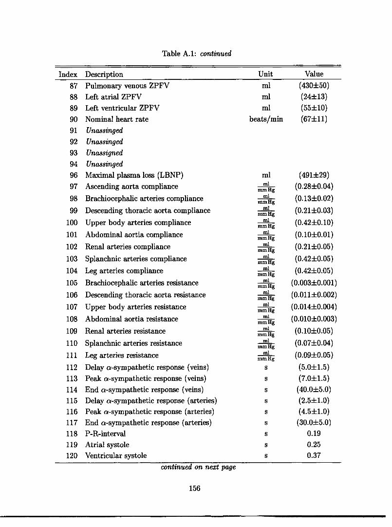
Table A.1: continued

Description

Pulmonary venous ZPFV

Left atrial ZPFV

Left ventricular ZPFV

Nominal heart rateUnassinged

UnassingedUnassignedUnassinged

Maximal plasma loss (LBNP)

Ascending aorta compliance

Brachiocephalic arteries compliance

Descending thoracic aorta compliance

Upper body arteries compliance

Abdominal aortia compliance

Renal arteries compliance

Splanchnic arteries compliance

Leg arteries compliance

Brachiocephalic arteries resistance

Descending thoracic aorta resistance

Upper body arteries resistance

Abdominal aortia resistance

Renal arteries resistance

Splanchnic arteries resistance

Leg arteries resistance

Delay a-sympathetic response (veins)

Peak a-sympathetic response (veins)

End a-sympathetic response (veins)

Delay a-sympathetic response (arteries)

Peak a-sympathetic response (arteries)

End a-sympathetic response (arteries)

P-R-interval

Atrial systole

Ventricular systole

Unitml

ml

ml

beats/min

mlml

mm Hgml

mm Hgml

mm Hgml

mm Hgml

mm Hgml

mm Hgml

mm Hgml

mm Hgml

mm Hgml

mm Hgml

mm Hgml

mm Hgml

mm Hgml

mm Hgml

mm Hg

S

S

S

S

S

S

S

S

S

Value

(430±50)

(24±13)

(55±10)

(67±11)

(491±29)

(0.28±0.04)

(0.13±0.02)

(0.21±0.03)

(0.42±0.10)

(0.10±0.01)

(0.21±0.05)

(0.42±0.05)

(0.42±0.05)

(0.003±0.001)

(0.011±0.002)

(0.014±0.004)

(0.010±0.003)

(0.10±0.05)

(0.07±0.04)

(0.09±0.05)

(5.0±1.5)

(7.0±1.5)

(40.0±5.0)

(2.5±1.0)(4.5±1.0)

(30.0±5.0)

0.19

0.25

0.37

continued on next page

156

Index

87

88

89

90

91

92

93

94

96

97

98

99

100

101

102

103

104

105

106

107

108

109

110

111

112

113

114

115

116

117

118

119

120

--

Table A.1: continued

Description

Ascending aorta (vertical length)

Brachiocephalic arteries (vertical length)

Upper body arteries (vertical length)

Upper body veins (vertical length)

Superior vena cava (vertical length)

Descending thoracic aorta (vertical length)

Abdominal aorta (vertical length)

Renal arteries (vertical length)

Renal veins (vertical length)

Splanchnic arteries (vertical length)

Splanchnic veins (vertical length)

Leg arteries (vertical length)

Leg veins (vertical length)

Abdominal veins (vertical length)

Inferior vena cava (vertical length)

Ascending aorta ZPFVBrachiocephalic arteries ZPFV

Descending thoracic aorta ZPFV

Upper body arteries ZPFVAbdominal aorta ZPFV

Renal arteries ZPFV

Splanchnic arteries ZPFV

Leg arteries ZPFV

Body height

Body weight

Body surface area

cm

cm

cm

cm

cm

cm

cm

cm

cm

cm

cm

cm

cm

cm

cm

ml

ml

ml

ml

ml

ml

ml

ml

cm

kgm 2

10.0

4.5

20.0

20.0

4.5

16.0

14.5

0

0

10.0

10.0

106

106

14.5

6.0

(21i3)(5+1)

(16+2)

(200+40)

(101)(20+5)

(300+50)

(200+20)

(169+1.5)

(70.3+2.1)

(1.83+0.02)

157

Index Unit Value

121

122

123

124

125

126

127

128

129

130

131

132

133

134

135

136

137

138

139

140

141

142

143

144

145

146

158

I

Appendix B

Allometry of the CardiovascularSystem

In Chapters 2 and 3, we have concerned ourselves with the architecture of and theparameter assignments for our cardiovascular model. In particular, we have assignednumerical values to the physical parameters of the model, assuming certain valuesfor anthropometric measures and cardiovascular variables. These values were deemedcharacteristic of the population we aim to represent (see Table 2.1). We referred tothis set of parameter values as the nominal parameter profile or the base state of themodel. We also strove to assess the degree of variability of each parameter valuewithin the population by estimating the respective standard errors.

The purpose of this appendix is to combine the nominal set of parameter valuesand their standard errors with general allometric scaling laws so we can generate pa-rameter profiles of subjects with different anthropometric and cardiovascular charac-teristics, as if they were recruited at random from a large population. This samplingwill enable us to repeat simulations for different subjects (i.e., different parameterprofiles) and therefore establish population-averaged responses.

Knowing the nominal parameter values and their standard deviations, we couldassume appropriate probability density functions (e.g., uniform, Gaussian, or log-normal) to sample each parameter independently. However, this sampling schemewould neglect important correlations that exist between physiological parameters:Figures B-1 and B-2 demonstrate that 'size matters' in physiological systems, wheresize is commonly quantified in terms of body weight. Figure B-1 demonstrates thatheight, and therefore gravitational stress, increases on average with increasing size.Figure B-2 shows that total blood volume also increases on average with increasingsize. In fact, most cardiovascular variables are extrinsic; their values scale with thesize of the organism, not only between different species but also intra-specifically(blood pressure being an important exception [265, p. 827]). Mathematically, thisphenomenon is described by allometric scaling laws, which take the form of power-law monomials

i = ai Wki (B.1)

where Yi is a physiological variable of interest such as, for example, basal metabolic

159

210

200

170

100

150

140

7000

A.a.., 'I. - - X ~~~~

:.:, . . i

I.

40 00 iO 70 s16 1 0 110 1240 I 40 s0 00 70 D 90 100

BodytWo!11 1odW)i

Figure B-l: Correlation of body height and Figure B-2: Correlation of total blood vol-body weight. Data adapted from [61]. ume and body weight. Data adapted from

[57].

rate, vascular compliance, limb length, or heart rate. W is the representative weightof an organism if one is interested in inter-specific variation of Y, or it can be theweight of different representatives of the same species if one is interested in intra-specific variation of Y. Pragmatically, the coefficient ai and the exponent ki bothhave to be estimated from data to establish the exact scaling law for the particularvariable Yi. This approach would not help us as we would need a large volume of datato correlate each parameter or class of parameters (compliances, resistances, volumes)to body weight.

Theoretical frameworks have been developed to predict the scaling exponents fordifferent physiological parameters, given a set of fundamental assumptions [266, 267].Two commonly used models are based on the principles of geometric and elastic sim-ilarity, respectively [268]. Geometric similarity is based on the assumption that a setof related animals have the same shape but differ in size. Mathematically, geometricsimilarity is based on proportional scaling of all variables of linear dimension. Inparticular, L oc D, where L is the dimension of a characteristic length variable (suchas the length of the femur), and D is the associated transverse dimension (such asthe diameter of the femur neck)l. Elastic similarity, on the other hand, asserts thatlarger animals are more strongly built than smaller ones [268]. In particular, it statesthat two variables are scaled in proportion to their characteristic elastic properties.Mathematically, elastic similarity is described by an affine transformation that scalesthe transverse dimensions relatively more than the longitudinal dimensions (L oc Ds).

If one assumes constant tissue density among or within species, weight scalesaccording to volume. W oc L D2 , so L oc W3 assuming geometric similarity andL c W4 when the model of elastic similarity is employed. Alternatively, D c W3and D oc Ws under the geometric and elastic model, respectively. By computingthe exponents ki for various anthropometric and cardiovascular variables, we candecide which of the two models is more appropriate in describing the population data

160

'The sign oc signifies proportionality.

____

:

m *

I-i.·· 8~

. .1

;...:·mnurr-

Table B.1: Allometric exponents of the human cardiovascular system.

Exponent k

Predicted Observedt

Geometric ElasticVariable Dimensions Geometric Elastic Referencesimilarity similarity

Body height L 0.333 0.250 (0.223 + 0.003) [61]0.333 0.250 (0.221 ± 0.026) [57]

Leg height L 0.333 0.250 (0.228 ± 0.004) [61]Chest circumference D 0.333 0.375 (0.405 ± 0.003) [61]Calf girth D 0.333 0.375 (0.347 ± 0.004) [61]Thigh girth D 0.333 0.375 (0.350 + 0.005) [61]Body surface area LD 0.667 0.625 (0.602 + 0.019) [57]Cardiac output LD2T - 1 0.667 0.75 0.71 [62]Blood volume LD2 1.0 1.0 (0.936 i 0.074) [57]tMean i standard error.

presented in Chapter 2. Table B.1 shows the results of the regression analysis andindicates that the data favor elastic over geometric similarity.

As mentioned above, blood pressure does not scale with body size, that is P oc W° .

Combining this information with the fact that blood volume scales proportional tobody size, we can determine that vascular compliance scales according to C oc W.To determine how resistance scales, we need to understand how blood flow scales.McMahon [268] argues and presents experimental confirmation that dynamic vari-ables of metabolic importance such as blood flow, minute respiration, and metabolicoxygen consumption all scale according to WI under the elastic similarity assump-tion. Resistance therefore scales as R oc W-4 and physiological time scales accordingto T c W .

To sample different parameter profiles from the population of subjects we are aim-ing to represent, we start with the nominal parameter profile and adopt the followingsampling and scaling strategy:

1. Sample from an empirical distribution function of body weights to obtain a newweight W1.

2. Normalize the nominal parameter 80 and its standard deviation a06 by theappropriately scaled nominal body weight W0:

Wi_ O-

as =

3. Sample a new normalized value 0~ from some appropriately chosen probabilitydistribution function Fi:

1 Fi(0, Ado)

161

4. Scale the new normalized parameter value by the appropriate power law toobtain the extensive value 01:

e = 1 w1

We chose the normal distribution for the sampling step (Step 2), but constrained thesamples to lie between pre-defined minima and maxima to account for the fact thatunder normal conditions, cardiovascular variables do not assume extremely large ornegative values.

162

Bibliography

[1] C.J. Dickinson. A digital computer model of the effects of gravitational stressupon the heart and venous system. Medical & Biological Engineering, 7:267-275, 1969.

[2] T.L. Ozawa, K.E. Bottom, X. Xiao, and R.D. Kamm. Numerical simula-tion of enhanced external counterpulsation. Annals of Biomedical Engineering,29(4):284-297, 2001.

[3] K. Peterson, E.T. Ozawa, G.M. Pantalos, and M.K. Sharp. Numerical simula-tion of the influence of gravity and posture on cardiac performance. Annals ofBiomedical Engineering, 30(2):247-259, 2002.

[4] V.K. Sud, R. Srinivasan, J.B. Charles, and M.W. Bungo. Effects of lower bodynegative pressure on blood flow with applications to the human cardiovascularsystem. Medical E4 Biological Engineering & Computing, 31(6):569-575, 1993.

[5] X. Xiao, E.T. Ozawa, Y. Huang, and R.D. Kamm. Model-based assessmentof cardiovascular health from noninvasive measurements. Annals of BiomedicalEngineering, 30(5):612-623, 2002.

[6] D.G. Boyers, J.G. Cuthbertson, and J.A. Luetscher. Simulation of the humancardiovascular system: A model with normal response to change in posture,blood loss, transfusion, and autonomic blockade. Simulation, 18:197-205, 1972.

[7] R.C. Croston, J.A. Rummel, and F.J. Kay. Computer model of cardiovascularcontrol system response to exercise. Journal of Dynamic Systems, Measurement,and Control, pages 301-307, 1973.

[8] R.W. DeBoer, J.M. Karemaker, and J. Stracke. Hemodynamic fluctuationsand baroreflex sensitivity in human: a beat-to-beat model. Journal of AppliedPhysiology, 253(3 Pt. 2):680-689, 1987.

[9] J.B. Madwed, P. Albrecht, R.G. Mark, and R.J. Cohen. Low-frequency oscilla-tions in arterial pressure and hear rate: a simple computer model. Journal ofApplied Physiology, 256(6 Pt 2):H1573-H1579, 1989.

163

[10] R.J. White, D.G. Fitzjerrell, and R.C. Croston. Cardiovascular modelling: Sim-ulating the human response to exercise, lower body negative pressure, zero grav-ity and clinical conditions. In Advances in Cardiovascular Physics, volume 5(Part I), pages 195-229. Karger, Basel, 1983.

[11] T.L. Davis. Teaching Physiology Through Interactive Simulation of Hemo-dynamics. Master's thesis, Department of Electrical Engineering and Com-puter Science, Massachusetts Institute of Technology, Cambridge, MA, Febru-ary 1991.

[12] T. Heldt, E.B. Shim, R.D. Kamm, and R.G. Mark. Computational modelingof cardiovascular response to orthostatic stress. Journal of Applied Physiology,92(3):1239-1254, 2002.

[13] M. Ursino. Interaction between carotid baroregulation and the pulsating heart:a mathematical model. Journal of Applied Physiology, 275(5 Pt. 2):H1733-H1747, 1998.

[14] R.J. White, D.G. Fitzjerrell, and R.C. Croston. Fundamentals of lumped com-partmental modelling of the cardiovascular system. In Advances in Cardiovas-cular Physics, volume 5 (Part I), pages 162-184. Karger, Basel, 1983.

[15] A.C. Guyton, T.C. Coleman, and H.J. Granger. Circulation: Overall regulation.Annual Review of Physiology, 34:13-46, 1972.

[16] R.C. Croston and D.G. Fitzjerrell. Cardiovascular model for the simulation ofexercise, lower body negative pressure, and tilt table experiments. In Proceed-ings of the Fifth Annual Pittsburgh Conference on Modeling and Simulation,pages 471-476, 1974.

[17] J.F. Green and N.C. Miller. A model describing the response of the circulatorysytem to acceleration stress. Annals of Biomedical Engineering, 1(4):455-467,1973.

[18] J.I. Leonard, C.S. Leach, and J.A. Rummel. Computer simulations of posturalchange, water immersion, and bedrest: An integrative approach for understand-ing the spaceflight response. Physiologist, 22(6):S31-S32, 1979.

[19] D. Jaron, T.W. Moore, and C.-L.C. Chu. A cardiovascular model for study-ing impairment of cerebral function during +Gz stress. Aviation, Space, andEnvironmental Medicine, 55(1):24-31, 1984.

[20] D. Jaron, T.W. Moore, and J. Bai. Cardiovascular response to accelerationstress: a computer simulation. Proceedings of the IEEE, 76(6):700-707, 1988.

[21] F.M. Melchior, R.S. Srinivasan, and J.M. Clbre. Mathematical modeling of thehuman response to LBNP. Physiologist, 35(1 Suppl.):S204-S205, 1992.

164

[22] F.M. Melchior, R.S. Srinivasan, P.H. Thullier, and J.M. Clere. Simulation ofcardiovascular response to lower body negative pressure from 0 to -40 mmHg.Journal of Applied Physiology, 77(2):630-640, 1994.

[23] K.E. Simanonok, R.S. Srinivasan, and J.B. Charles. A computer simulationstudy of preadaptation of the circulation by removal of different blood volumesto counteract fluid shifts. Physiologist, 35(1 Suppl.):S111-S112, 1992.

[24] K.E. Simanonok, E.E. Srinivasan, R.S. Myrick, A.L. Blomkalns, and J.B.Charles. A comprehensive guyton model analysis of physiologic responses topreadapting the blood volume as a countermeasure to fluid shifts. Journal ofClinical Pharmacology, 34(5):440-453, 1994.

[25] M.F. Snyder and V.C Rideout. Computer simulation studies of the venouscirculation. IEEE Transactions on Biomedical Engineering, BME-16(4):325-334, 1969.

[26] R.S. Srinivasan, K.E. Simanonok, and J.B. Charles. Computer simulation anal-ysis of the effects of countermeasures for reentry orthostatic intolerance. Phys-iologist, 35(1 Suppl.):S165-S168, 1992.

[27] R.J. White, J.I. Leonard, R.S. Srinivasan, and J.B. Charles. Mathematicalmodeling of acute and chronic cardiovascular changes during extended durationorbiter (EDO) flights. Acta Astronautica, 23:41-51, 1991.

[28] R.J. White and C.G. Blomqvist. Central venous pressure and cardiac functionduring spaceflight. Journal of Applied Physiology, 85(2):738-746, 1998.

[29] Consensus Committee of the American Autonomic Society and the AmericanAcademy of Neurology. Consensus statement on the definition of orthostatichypotension, pure autonomic failure and multiple system atrophy. ClinicalAutonomic Research, 6:125-126, 1996.

[30] J.V. Meck, C.J. Reyes, S.A. Perez, A.L. Goldberger, and M.G. Ziegler. Markedexacerbation of orthostatic intolerance after long- vs. short-duration spaceflightin veteran astronauts. Psychosomatic Medicine, 63(6):865-873, 2001.

[31] T.L. Davis and R.G. Mark. Teaching physiology through simulation of hemo-dynamics. Computers in Cardiology, 17:649-652, 1990.

[32] J.L. Chang. Cycle-averaged models of cardiovascular dynamics. Master's thesis,Department of Electrical Engineering and Computer Science, MassachusettsInstitute of Technology, Cambridge, MA, June 2002.

[33] J.J.S. Chen. Analytical solution to a simplified circulatory model using piece-wise linear elastance function. Master's thesis, Department of Electrical En-gineering and Computer Science, Massachusetts Institute of Technology, Cam-bridge, MA, July 2003.

165

[34] J.J.S. Chen, T. Heldt, G.C. Verghese, and R.G. Mark. Analytical solutionto simplified circulatory model using piecewise linear elastance. Computers inCardiology, 30:45-48, 2003.

[35] T. Heldt, J.L. Chang, G.C. Verghese, and R.G. Mark. Cycle-averaged modelsof cardiovascular dynamics. In D.D. Feng and E.R. Carson, editors, Modellingand Control in Biomedical Systems 2003, pages 387-391, Oxford, UK, 2003.International Federation of Automatic Control, Pergamon.

[36] G. Jacob, A.C. Ertl, J.R. Shannon, R. Furlan, R.M. Robertson, and D. Robert-son. Effect of standing on neurohumoral responses and plasma volume in healthysubjects. Journal of Applied Physiology, 84(3):914-921, 1998.

[37] Critical Path Control Panel. Critical Path Roadmap (CPR) Baseline Document.<http://criticalpath.jsc.nasa.gov>, 2000. Website accessed on July 08, 2003.

[38] J.M. Fritsch-Yelle, J.B. Charles, M.M. Jones, L.A. Beightol, and D.L. Eckberg.Spaceflight alters autonomic regulation of arterial pressure in humans. Journalof Applied Physiology, 77(4):1776-1783, 1994.

[39] C.M. Lathers and J.B. Charles. Orthostatic hypotension in patients, bedrestsubjects, and astronauts. Journal of Clinical Pharmacology, 28(10 Suppl.):S29-S32, 1994.

[40] J.V. Tyberg and D.R. Hamilton. Orthostatic hypotension and the role ofchanges in venous capacitance. Medicine and Science in Sports and Exercise,28(10 Suppl.):S29-S31, 1996.

[41] B.D. Levine, J.H. Zuckerman, and J.A. Pawelczyk. Cardiac atrophy afterbedrest deconditioning: A nonneural mechanism for orthostatic intolerance.Circulation, 96(2):517-525, 1997.

[42] M.A. Perhonen, F. Franco, L.D. Lane, J.C. Buckey, C.G. Blomqvist, J.E. Zerk-wekh, R.M. Peshock, P.T. Weatherall, and B.D. Levine. Cardiac atrophy afterbed rest and spaceflight. Journal of Applied Physiology, 91(2):645-653, 2001.

[43] M.A. Perhonen, J.H. Zuckerman, and B.D. Levine. Deterioration of left ven-tricular chamber performance after bed rest: "cardiovascular deconditioning"or hypovolemia? Circulation, 103(14):1851-1857, 2001.

[44] D.S. Martin, D.A. South, M.L. Wood, M.W. Bungo, and J.V. Meck. Compar-ison of echocardiographic changes after short- and long-duration spaceflight.Aviation, Space, and Environmental Medicine, 73(6):532-536, 2002.

[45] J.C. Buckey, L.D. Lane, G. Plath, F.A. Gaffney, F. Baisch, and C.G. Blomqvist.Effects of head-down tilt for 10 days on the compliance of the leg. Acta Physi-ologica Scandandinavica, 144(S604):53-60, 1992.

166

[46] D. Robertson, V.A. Convertino, and J. Vernikos. The sympathetic nervoussystem and the physiologic consequences of spaceflight: a hypothesis. TheAmerican Journal of the Medical Sciences, 308(2):126-132, 1994.

[47] B.J. Yates and I.A. Kerman. Post-spaceflight orthostatic intolerance: Possiblerelationship to microgravity induced plasticity in the vestibular system. BrainResearch Reviews, 28(1-2):73-82, 1998.

[48] C.G. Blomqvist, J.C. Buckey, F.A. Gaffney, L.D. Lane, J.D. Levine, and D.E.Watenpaugh. Mechanisms of post-flight orthostatic intolerance. Journal ofGravitational Physiology, 1(1):P122-P124, 1994.

[49] C.G. Blomqvist. Regulation of the systemic circulation at microgravity andduring readaptation to 1 G. Medicine and Science in Sports and Exercise,28(10 Suppl.):S9-S13, 1996.

[50] S.L. Mulvagh, J.B. Charles, J.M. Riddle, T.L. Rehbein, and M.W. Bungo.Echocardiographic evaluation of the cardiovascular effects of short-durationspaceflight. Journal of Clinical Pharmacology, 31(10):1024-1026, 1991.

[511 P.A. Whitson, J.B. Charles, W.J. Williams, and N.M. Cintr6n. Changes insympathoadrenal response to standing in humans after spaceflight. Journal ofApplied Physiology, 79(2):428-433, 1995.

[52] J.M. Fritsch-Yelle, J.B. Charles, M.M. Jones, and M.L. Wood. Microgravitydecreases heart rate and arterial pressure in humans. Journal of Applied Phys-iology, 80(3):910-914, 1996.

[53] J.C. Buckey, L.D. Lane, J.D. Levine, D.E. Watenpaugh, S.J. Wright, W.E.Moore, F.A. Gaffney, and C.G. Blomqvist. Orthostatic intolerance after space-flight. Journal of Applied Physiology, 81(1):7-18, 1996.

[54] L.F. Zhang. Vascular adaptation to microgravity: What have we learned?Journal of Applied Physiology, 91(6):2415-2430, 2001.

[55] J.G. Defares, J.J. Osborn, and H.H. Hara. Theoretical synthesis of the cardio-vascular system. Study I: The controlled system. Acta physiologica et pharma-cologica Neerlandica, 12:189-265, 1963.

[56] R.W. Leggett and L.R. Williams. A proposed blood cicrulation model for ref-erence man. Health Physics, 69(2):187-201, 1995.

[57] J.G. Gibson, 2nd and W.A. Evans, Jr. Clinical studies of the blood volume.II The relation of plasma and total blood volume to venous pressure, bloodvelocity rate, physical measurements, age and sex in ninety normal humans.Journal of Clinical Investigation, 16:317-328, 1937.

167

[58] A. Cournand, R.L. Riley, E.S. Breed, E. deF. Baldwin, and D.W. Richards, Jr.Measurement of cardiac output in man using the technique of catheterization ofthe right auricle or ventricle. Journal of Clinical Investigation, 24(1):106-116,1945.

[59] J.M. Tanner. The construction of normal standards for cardiac output in man.Journal of Clinical Investigation, 28:567-582, 1949.

[60] B.G. Barratt-Boyes and E.H. Wood. Cardiac output and related measurementsand pressure values in the right heart and associated vessels, together withan analysis of the hemodynamic response to the inhalation of hight oxygenmixtures in healthy subjects. The Journal of Laboratory and Clinical Medicine,51(1):72-90, 1958.

[61] Human Systems Information Center. 1988 Anthropometric Survey ofthe U.S. Army Male/Female Working Data Set. Technical report,U.S. Department of Defense, Wright-Patterson Air Force Base, OH.<http://iac.dtic.mil/hsiac/AnthroUSMilitary.htm>; website accessed on 9April 2004.

[621 G. de Simone, R.B. Devereux, S.R. Daniels, G. Mureddu, M.J. Roman, T.R.Kimball, R. Greco, S. Witt, and F. Contaldo. Stroke volume and cardiac outputin normotensive children and adults. Circulation, 95(7):1837-1843, 1997.

[63] P.L. Williams, editor. Gray's Anatomy. Churchill Livingstone, New York, 38edition, 1995.

[64] F. Martini. Human Anatomy. Prentice Hall, Upper Saddle River, New Jersey,2nd edition, 1997.

[65] International Commission on Radiological Protection. Report of the Task Groupon Reference Man. ICRP publication 23. Pergamon Press, New York, 1975.

[66] C. Macchi and C. Catini. The use of ultrasonic tomography to measure the cal-ibers of the iliac arteries and veins and the caliber an dlength of the inferior venacava and the abdominal aorta. Italian Journal of Anatomy and Embryology,99(3):181-186, 1994.

[67] P. Bonnichon, F. Gaudard, E. Ouakil, P. Lebozec, C. de Labrouhe, A. Bonnin,C. Aaron, and Y. Chapuis. Biometry of infrarenal inferior vena cava mea-sured by cavography. Clinical applications. Surgical and Radiologic Anatomy,11(2):149-154, 1989.

[68] United States of America Department of Defense. Anthropometry of U.S. mili-tary personnel (metric). Military Handbook DOD-HDBK-743A, United StatesDepartment of Defense, 1991. <http://iac.dtic.mil/hsiac/StdHdbk.htm>:website accessed on 10 February 2004.

168

[69] A.P. Avolio. Multi-branched model of the human arterial system. Medical &Biological Engineering & Computing, 18(6):709-718, 1980.

[70] A. Noordergraaf, P.D. Verdouw, and H.B. Boom. The use of an analog computerin a circulation model. Progress in Cardiovascular Diseases, 5(5):419-439, 1963.

[71] J.W. Remington and W.F. Hamilton. The construction of a theoretical cardiacejection curve from the contour of the aortic pressure pulse. American Journalof Physiology, 144:546-556, 1945.

[72] P. Hallock and J.C. Benson. Studies on the elastic properties of human isolatedaorta. American Journal of Physiology, 16:595-602, 1937.

[73] A.A. Pollack and E.H. Wood. Venous pressure in the saphenous vein at the anklein man during exercise and changes in posture. Journal of Applied Physiology,1:649-662, 1949.

[74] D.J. Griffiths. Principles of blood flow through collapsible tubes. In A.M.N.Gardner and R.H Fox, editors, The return of blood to the heart: venous pumpsin health and disease, pages 159-170. John Libbey & Company Ltd., London,1993.

[75] J.P. Henry. The significance of the loss of blood volume into the limbs duringpressure breathing. Aviation Medicine, 22(1):13-38, 1951.

[76] H.W. Ryder, W.E. Molle, and E.B. Ferris, Jr. The influence of the collapsibilityof veins on venous pressure, including a new procedure for measureing tissuepressures. Journal of Clinical Investigation, 23(3):333-342, 1943.

[77] R.W. Leggett and L.R. Williams. Suggested reference values for regional bloodvolumes in humans. Health Physics, 60(2):139-154, 1991.

[78] F. Karim and R. Hainsworth. Responses of abdominal vascular capacitance tostimulation of splanchnic nerves. American Journal of Physiology, 231(2):434-440, 1976.

[79] C.F. Rothe. Venous system: physiology of the capacitance vessels. In T.J.Shepard, F.M. Abboud, and S.R. Geiger, editors, The cardiovascular system:peripheral circulation and organ blood flow, volume III of Handbook of Physiol-ogy, chapter 13, pages 397-452. American Physiological Society, Bethesda, MD,1983.

[80] L.B. Rowell. Human Cardiovascular Control, chapter 6. Oxford UniversityPress, New York, NY, 1993.

[81] M.W. Bleeker, P.C.E. De Groot, J.A. Pawelczyk, M.T.E. Hopman, and B.D.Levine. Effects of 18 days of bed rest on leg and arm venous properties. Journalof Applied Physiology, 96(3):840-847, 2004.

169

[82] C.C. Arnoldi and H. Linderholm. Venous blood pressures in the lower limb atrest and during exercise in patients with idiopathic dysfunction of the venouspump in the calf. Acta Chirurgica Scandinavica, 135(7):601-609, 1969.

[83] M.F. O'Rourke. Arterial function in health and disease. Chruchill, Edinburgh,1982.

[84] H. Suga. Time course of left ventricular pressure-volume relationship undervarious end-diastolic volumes. Japanese Heart Journal, 10(6):509-515, 1969.

[85] H. Suga. Time course of ventricular pressure-volume relationship under variousextends of aortic occlusion. Japanese Heart Journal, 11(4):373-378, 1970.

[86] H. Suga. Left ventricular time-varying pressure/volume ratio in systole as anindex of myocardial inotropism. Japanese Heart Journal, 12(2):153-160, 1971.

[87] H. Suga, K. Sagawa, and A.A. Shoukas. Load independence of the instantaneouspressure-volume ratio of the canine left ventricle and effects of epinephrine andheart rate on this ratio. Criculation Research, 32(3):314-322, 1973.

[88] H. Senzaki, C. Chen, and D.A. Kass. Single beat eatimation of end-systolicpressure-volume relations in humans. Circulation, 94(10):2497-2506, 1996.

[89] R.G. McKay, J.M. Aroesty, G.V. Heller, H.D. Royal, S.E. Warren, andW. Grossman. Assessment of the end-systolic pressure-volume relationship inhuman beings with the use of a time-varying elastance model. Circulation,74(1):97-104, 1986.

[90] W. Grossman, E. Braunwald, T. Mann, L.P. McLaurin, and L.H. Green. Con-tractile state of the left ventricle in man as evaluated from end-systolic pressure-volume relations. Circulation, 56(5):845-852, 1977.

[91] M.R. Starling, R.A. Walsh, L.J. Dell'Italia, G.B.J. Manchini, J.C. Lasher, andJ.L. Lancaster. The relationship of various measures of end-systole to left ven-tricular maximum time-varying elastance in man. Circulation, 76(1):32-43,1987.

[92] L.J. Dell'Italia and R.A. Walsh. Application of a time varying elastance modelof right ventricular performance in man. Cardiovascular Research, 22(12):864-874, 1988.

[93] J.M. Dernellis, C.I. Stefanadis, A.A. Zacharoulis, and P.K. Toutouzas. Leftatrial mechanical adaptation to long-standing hemodynamic loads based onpressure-volume relations. American Journal of Cardiology, 81(9):1138-1143,1998.

[94] J. Alexander, Jr., K. Sunagawa, N. Chang, and K. Sagawa. Instantaneouspressure-volume relation of the ejecting canine left atrium. Circulation Research,61(2):209-219, 1987.

170

[95] F. Schwiep, S.S. Cassidy, M. Ramanathan, and R.L. Johnson, Jr. Rapid in vivodeterminations of instantaneous right ventricular pressure and volume in dogs.American Journal of Physiology, 254(23):H622-H630, 1988.

[96] V.-K. Lau, K. Sagawa, and H. Suga. Instantaneous pressure-volume relationshipof right atrium during isovolumic contraction in canine heart. American Journalof Physiology, 236(5):H672-H679, 1979.

[97] M.S. Firstenberg, P.M. Vandervoot, N.L. Greenberg, N.G. Smedira, P.M. Mc-Carthy, M.J. Garcia, and J.D. Thomas. Noninvasive estimation of transmitralpressure drop across the normal mitral valve in humans: importance of convec-tive and inertial forces during left ventricular filling. Journal of the AmericanCollege of Cardiology, 36(6):1942-1949, 2000.

[98] H.C. Bazett. An analysis of the time-relations of electrocardiograms. Heart,7:353-370, 1920.

[99] K. Sagawa, L. Maughan, H. Suga, and K. Sunegawa. Cardiac contraction andthe pressure-volume relationship. Oxford University Press, New York, 1988.

[100] E.T. Ozawa. A numerical model of the cardiovascular system for clinical assess-ment of the hemodynamic state. Doctoral dissertation, Massachusetts Instituteof Technology, Cambridge, MA, September 1996.

[101] L.D. Nguyen and C.L. Leger. Four-dimensional reconstruction of the left ventri-cle using a fast rotating classical phased array scan head: Preliminary results.Journal of the American Society of Echocardiography, 15(6):593-600, 2002.

[102] F.P. Knowlton and E.H. Starling. The influence of variations in temperature andblood pressure on the performance of the isolated mammalian heart. Journalof Physiology, 44(3):206-219, 1912.

[103] R.W. Brower and A. Noordergraaf. Pressure flow characteristics of collapsibletubes: A reconciliation of seemingly contradictory results. Annals of Bioengi-neering, 1(3):333-335, 1973.

[104] J.B. West, C.T. Dollery, and A. Naimark. Distribution of blood flow in isolatedlung; relation to vascular and alveolar pressure. Journal of Applied Physiology,19(4):713-724, 1964.

[105] S. Permutt and R.L. Riley. Hemodynamics of collapsible vessels with tone: thevascular waterfall. Journal of Applied Physiology, 18(5), 1963.

[106] A. Shapiro. Steady flow in collapsible tubes. Journal of Biomechanical Engi-neering, 99:126-147, 1977.

[107] R.D. Kamm. Flow through collapsible tubes. In R. Skalak and S. Chien, editors,Handbook of Bioengineering, chapter 23, pages 23.1-23.19. McGraw-Hill, NewYork, 1987.

171

[108] S. Permutt, B. Bromberger-Barnea, and H.N. Bane. Alveolar pressure, pul-monary venous pressure, and the vascular waterfall. Medicina Thoracalis,19:239-260, 1962.

[109] M.L. Lewis and L.C Christianson. Behavior of the human pulmonary circulationduring head-up tilt. Journal of Applied Physiology, 45(2):249-254, 1978.

[110] L. Dexter, J.W. Dow, F.W. Haynes, J.L. Whittenberger, B.G. Ferris, W.T.Goodale, and H.K. Hellems. Studies of the pulmonary circulation in man atrest. Normal variations and the interrelations between increased pulmonaryblood flow, elevated pulmonary arterial pressure, and high pulmonary "capil-lary" pressures. Journal of Clinical Investigation, 29:602-613, 1950.

[111] R.N. Westcott, N.O. Fowler, R.C. Scott, V.D. Hauenstein, and J. McGuire.Anoxia and human pulmonary vascular resistance. Journal of Clinical Investi-agtion, 30(9):957-970, 1951.

[112] W.R. Milnor, A.D. Jose, and C.J. McGaff. Pulmonary vascular volume, resis-tance, and compliance in man. Circulation, 22:130-137, 1960.

[113] S.R. Reuben. Compliance of the human pulmonary arterial system in disease.Circulation Research, 29(1):40-50, 1971.

[114] A.C. Gutyon and J.E. Hall. Textbook of Medical Physiology. W.B. Saunders,Philadelphia, 10th edition, 2000.

[115] J.E.W. Beneken and B. DeWitt. A physical approach to hemodynamic aspectsof the human cardiovascular system. In A.C. Guyton and E.B. Reeve, editors,Physical bases of circulatory transport: Regulation and exchange, pages 1-45.W.B. Saunders, Philadelphia, 1967.

[116] S. Hirakawa. Capacitance of systemic and pulmonary circulatory system duringacute venous congestion. Japanese Circulation Journal, 37(7):753-760, 1973.

[117] S. Hirakawa, H. Ito, A. Sakai, and A. Wakabayashi. Estimation of the com-pliance of the human "venous" system from pulmonary artery wedge pressuretracings. Japanese Circulation Journal, 45(1):15-23, 1981.

[118] T. Tanaka, M. Arakawa, T. Suzuki, M. Gotoh, H. Miyamoto, and S. Hirakawa.Compliance of human pulmonary "venous" system estimated from pulmonaryartery wedge pressure tracings. Japanese Circulation Journal, 50(2):127-139,1986.

[119] R.V. Ebert, C.W. Borden, H.S. Wells, and R.H. Wilson. Studies of the pul-monary circulation. I. The circulation time from the pulmonary artery to thefemoral artery and the quantity of blood in the lungs in normal individuals.Journal of Clinical Investigation, 28:1134-1137, 1949.

172

[120] A.C. Burton. Physiology and Biophysics of the Circulation. Chicago Year BookMedical Publishers, 2 edition, 1972.

[121] W.R. Milnor. Pulmonary hemodynamics. In D.H. Bergel, editor, CardiovascularFluid Dynamics, pages 299-340. Academic Press, London, 1972.

[122] W.J. Daly and S. Bondurant. Direct measurement of respiratory pleural pres-sure changes in normal man. Journal of Applied Physiology, 18(3):513-518,1963.

[123] J. Mead and E.A. Gaensler. Esophageal and pleural pressures in man, uprightand supine. Journal of Applied Physiology, 14(1):81-83, 1959.

[124] B.G. Ferris, Jr., J. Mead, and N.R. Frank. Effect of body position on esophagealpressure and measurement of pulmonary compliance. Journal of Applied Phys-iology, 14(4):521-524, 1959.

[125] J. Lundvall, P. Bjerkhoel, S. Quittenbaum, and P. Lindgren. Rapid plasma vol-ume decline upon quiet standing reflects large filtration capacity in dependentlimbs. Acta Physiologica Scandinavica, 158(2):161-167, 1996.

[126] R.C. Tarazi, H.J. Melsher, H.P. Dustan, and E.D. Frohlich. Plasma volumechanges with upright tilt: studies in hypertension and in syncope. Journal ofApplied Physiology, 28(2):121-126, 1970.

[127] H. Hinghofer-Szalkay and M. Moser. Fluid and protein shifts after posturalchanges in humans. American Journal of Physiology, 250(19):H68-H75, 1986.

[128] R.D. Hagan, F.J. Diaz, and S.M. Horvath. Plasma volume changes with move-ment to the upright position. Journal of Applied Physiology, 45(3):414-417,1978.

[129] J. Lundvall and P. Bjerkhoel. Failure of hemoconcentration during standing toreveal plasma volume decline induced in the erect posture. Journal of AppliedPhysiology, 77(5):2155-2162, 1994.

[130] P. Bjerkhoel and J. Lundvall. Rapid and large plasma volume decrease uponshort-term quiet standing. Acta Physiologica Scandinavica, 150(3):347-348,1994.

[131] P. Bjerkhoel and J. Lundvall. Pronounced plasma fluid loss into dependentregions on standing. Acta Physiologica Scandinavica, 154(2):275-276, 1995.

[132] J. Lundvall and P. Bjerkhoel. Pronounced and rapid plasma volume reductionupon quite standing as revealed by a novel approach to the determination of theintravascular volume change. Acta Physiologica Scandinavica, 154(2):131-142,1995.

173

[133] J. Lundvall and P. Lindgren. F-cell shift and protein loss strongly affect validityof PV reductions indicated by Hb/Hct and plasma proteins. Journal of AppliedPhysiology, 84(3):822-829, 1998.

[134] C.C. Arnoldi. Venous pressures in the leg of healthy human subjects at restand during muscular exercise in the nearly erect position. Acta ChirurgicaScandinavica, 130:570-583, 1965.

[135] H. Tanaka, B.J. Sjbberg, and 0. Thulesius. Cardiac output and blood pressureduring active and passive standing. Clinical Physiology, 16(2):157-170, 1996.

[136] R.L.H. Sprangers, K.H. Wesseling, A.L.T. Imholz, B.P.M. Imholz, and W. Wiel-ing. Initial blood pressure fall on stand up and exercise explained by changes intotal peripheral resistance. Journal of Applied Physiology, 70(2):523-530, 1991.

[137] J. Lundvall, P. Bjerkhoel, C. Ivarsson, and T. Linne. Dynamics of transcapillaryfluid transfer and plasma volume during lower body negative pressure. ActaPhysiologica Scandinavica, 147(2):163-172, 1993.

[138] M. Aratow, S.M. Fortney, D.E. Watenpaugh, A.G. Crenshaw, and A.R. Har-gens. Transcapillary fluid responses to lower body negative pressure. Journalof Applied Physiology, 74(6):2763-2770, 1993.

[139] W.H. Press, S.A. Teukolsky, W.T. Vetterling, and B.P. Flannery. Numericalrecipes in C: the art of scientific computing, chapter 16, pages 707-747. Cam-bridge University Press, New York, NY, 2nd edition, 1992.

[140] R.W. de Boer. Beat-to-beat blood-pressure fluctuations and heart-rate variabil-ity in man: physiological relationships, analysis techniques and a simple model.Doctoral dissertation, Department of Physiology, University of Amsterdam,Amsterdam, The Netherlands, December 1985.

[141] R. Mukkamala. A Forward Model-Based Analysis of Cardiovascular SystemIdentification Methods. Doctoral dissertation, Massachusetts Institute of Tech-nology, Cambridge, MA, June 2000.

[142] G. Mancia and A.L. Mark. Arterial baroreflex in humans. In T.J. Shepard, F.M.Abboud, and S.R. Geiger, editors, The peripheral circulation, volume III (Part2) of Handbook of Physiology, Section 2: The Cardiovascular System, chap-ter 20, pages 755-793. American Physiological Society, Bethesda, MD, 1983.

[143] R.D. Berger. Analysis of the Cardiovascular Control System using Broad-Band Stimulation. Doctoral dissertation, Massachusetts Institute of Technology,Cambridge, MA, June 1987.

[144] R.D. Berger, J.P. Saul, and R.J. Cohen. Transfer function analysis of auto-nomic regulation I. Canine atrial rate response. American Journal of Physiol-ogy, 256(25):H142-H152, 1989.

174

[145] C. Borst and J.M. Karemaker. Time delays in the human baroreflex. Journalof the Autonomic Nervous System, 9(2-3):399-409, 1983.

[146] D.L. Eckberg. Nonlinearities of the human carotid baroreceptor-cardiac reflex.Circulation Research, 47(2):208-216, 1980.

[147] R.F. Rea and D.L. Eckberg. Carotid baroreceptor-muscle sympathetic relationin humans. American Journal of Physiology, 253(22):R929-R934, 1987.

[148] C. Keyl, A. Schneider, M. Dambacher, and L. Bernardi. Time delay of vagallymediated cardiac baroreflex response varies with autonomic cardiovascular con-trol. Journal of Applied Physiology, 91(1):283-289, 2001.

[149] M. Rosenbaum and D. Race. Frequency-response characteristics of vascularresistance vessels. American Journal of Physiology, 215(6):1397-1402, 1968.

[150] A.A. Shoukas, C.L. MacAnespie, M.J. Brunner, and L. Watermeier. The im-portance of the spleen in blood volume shifts of the systemic vascular bedcaused by the carotid sinus baroreceptor reflex in the dog. Circulation Re-search, 49(3):759-766, 1981.

[151] T.J. Mullen, M.L. Appel, R. Mukkamala, J.M. Mathias, and R.J. Cohen. Sys-tem identification of closed-loop cardiovascular control: effects of posture andautonomic blockade. American Journal of Physiology, 272(Heart Circ. Physiol.41):H448-H461, 1997.

[152] R. Mukkamala, K. Toska, and R.J. Cohen. Noninvasive identification ofthe total peripheral resistance baroreflex. American Journal of Physiology,284(3):H947-H959, 2002.

[153] P.G. Katona and G.O. Barnett. Central origin of asymmetry in the carotid sinusreflex. Annals of the New York Academy of Sciences, 156(2):779-786, 1969.

[154] J.D. Bistow, A.J. Honour, T.G. Pickering, and P. Sleight. Cardiovascular andrespiratory changes during sleep in normal and hypertensive subjects. Cardio-vascular Research, 3:476-485, 1969.

[155] D.L. Eckberg, M. Drabinsky, and E. Braunwald. Defective cardiac parasympa-thetic control in patients with heart disease. New England Journal of Medicine,285(16):877-883, 1971.

[156] T.G. Pickering, B. Gribbin, and P. Sleight. Comparison of the reflex heart rateresponse to rising and falling arterial pressure in man. Cardiovascular Research,6(2):277-283, 1972.

[157] T.G. Pickering, B. Gribbin, E. Strange Petersen, D.J.C. Cunningham, andP. Sleight. Effects of autonomic blockade on the baroreflex in man at restand during exercise. Circulation Research, 30:177-185, 1972.

175

[158] P.I. Korner, M.J. West, J. Shaw, and J.B. Uther. 'Steady State' properties ofthe baroreceptor-heart rate reflex in essential hypertension in man. Clinical andExperimental Pharmacology and Physiology, 1:65-76, 1974.

[159] R.W. de Boer, J.M. Karemaker, and J. Stracke. Description of heart rate vari-ability data in accordance with a physiological model of the genesis of heart-beats. Psychophysiology, 22(2):147-155, 1985.

[160] B. Ahn, Y. Skakibara, P. Paulev, A. Masuda, Y. Nishibayashi, W. Nakamura,and Y. Honda. Circulatory and respiratory response to lower body negativepressure in man. Japanese Journal of Physiology, 39:919-929, 1989.

[161] C.M. Brown, M. Diitsch, M.J. Hecht, B. Neund6rfer, and M.J. Hilz. Assessmentof cerebrovascular and cardiovascular responses to lower body negative pressureas a test of cerebral autoregulation. Journal of the Neurological Society, 208(1-2):71-78, 2003.

[162] A.A. Shoukas and M.C. Brunner. Epinepherine and the carotid sinus reflex:Influence on capacitive and resistive properties of the total systemic vascularbed of the dog. Circulation Research, 47(2):249-257, 1980.

[163] R.M. Berne and M.N. Levy. Cardiovascular Physiology. Mosby-Year Book, Inc.,St. Louis, MI, 7 edition, 1997.

[164] A.L. Mark and G. Mancia. Cardiopulmonary baroreflexes in humans. In T.J.Shepard, F.M. Abboud, and S.R. Geiger, editors, The peripheral circulation,volume III (Part 2) of Handbook of Physiology, Section 2: The CardiovascularSystem, chapter 21, pages 795-813. American Physiological Society, Bethesda,MD, 21 edition, 1983.

[165] J.M. Johnson, L.B. Rowell, M. Niederberger, and M.M. Eisman. Humansplanchnic and forearm vasoconstrictor responses to reductions of right atrialand aortic pressure. Circulation Research, 34(4):515-524, 1974.

[166] J.A. Pawelczyk and P.B. Raven. Reductions in central venous pressure improvecarotid baroreflex responses in concious men. American Journal of Physiology,257(Heart Circ. Physiol. 26):H1389-H1395, 1989.

[167] T.H. Desai, J.C. Collins, M. Snell, and R. Mosqueda-Garcia. Modeling of ar-terial and cardiopulmonary baroreflex control of heart rate. American Journalof Physiology, 1997(Heart Circ. Physiol. 41):H2342-H2352, 1997.

[168] H.L. Price. Hemodynamic and metabolic effects of hemorrhage in man withparticular reference to the splanchnic circulation. Circulation Research, 18:469-474, 1966.

[169] S. Bevegard, J. Castenfros, and L.E. Lindblad. Effects of changes in bloodvolume distribution on circulatory variables and plasma rening activity. ActaPhysiologica Scandinavica, 99(2):237-245, 1977.

176

[170] W. Giles, D.A. Eisner, and W.J. Lederer. Sinus pacemaker activity in the heart.In David O. Carpenter, editor, Cellular Pacemakers, volume 1, chapter 3. JohnWiley & Sons, New York, 1982.

[171] H.H. Hecht. Comparative physiological and morphological aspects of pacemakertissues. Annals of the New York Academy of Sciences, 127:49-83, 1965.

[172] S. Akselrod, D. Gordon, F.A. Ubel, D.C. Shannon, C. Barger, and R.J. Cohen.Power spectrum analysis of heart rate fluctuation: a quantitative probe of beat-to-beat cardiovascular control. Science, 213(4504):220-222, 1981.

[173] B.W. Hyndman and R.K. Mohn. A model of the cardiac pacemaker and its usein decoding the information content of cardiac intervals. Automedica, 1:239-252,1975.

[174] R.A. Bloomfield, H.D. Lauson, A. Cournand, E.S. Breed, and D.W. Richards,Jr. Recording of right heart pressures in normal subjects and in patients withchronic pulmonary disease and various types of cardio-circulatory disease. TheJournal of Clinical Investigation, 25(5):639-664, 1946.

[175] N.O. Fowler, R.N. Westcott, and R.C. Scott. Normal pressure in the right heartand pulmonary artery. American Heart Journal, 46:264-267, 1953.

[176] E. Braunwald, E.C. Brockenbrough, C.J. Frahm, and J. Ross. Left atrial and leftventricular pressures in subjects without cardiovascular disease: Observations ineighteen patients studied by transseptal left heart catheterization. Circulation,24:267-269, 1961.

[177] J.W. Kennedy, W.A. Baxley, M.M. Figley, H.T. Dodge, and J.R. Blackmon.Quantitative angiocardiography: I. The normal left ventricle. Circulation,34(2):272-278, 1966.

[178] F. Cucchini, C. Di Mario, A. Iavernaro, R. Zeppellini, A. Barilli, and R. Bolog-nesi. Peak aortic blood acceleration: a possible indicator of initial left ven-tricular impairment in patients with coronary artery disease. European HeartJournal, 12(8):860-868, 1991.

[179] W.W. Nichols and M.F. O'Rourke. McDonald's Blood Flow in Arteries: Theo-retical, practical and clinical principles. Arnold, London, 4 edition, 1998.

[180] Y.C. Fung. Biodynamics - Circulation. Springer-Verlag, New York, 1984.

[181] C.G. Caro, T.J. Pedley, R.C. Schroter, and W.A. Seed. The Mechanics of theCirculation. Oxford Medical Publishers, Oxford University Press, New York,1978.

[182] M. Kumada, T. Azuma, and K. Matsuda. The cardiac output-heart raterelationship under different conditions. The Japanese Journal of Physiology,17(5):538-555, 1967.

177

[183] J.J. Smith, C.V. Hughes, M.J. Ptacin, J.A. Barney, F.E. Tristani, and T. J.Ebert. The effect of age on hemodynamic response to graded postural stress innormal men. Journal of Gerontology, 42(4):406-411, 1987.

[184] O.H. Gauer and H.L. Thron. Postural changes in the circulation. In W.F.Hamilton, editor, Handbook of Physiology, volume 3, chapter 67, pages 2409-2439. American Physiological Society, 1965.

[185] J. Hisdale, K. Toska, and L. Wall0e. Beat-to-beat cardiovascular responsesto rapid, low-level LBNP in humans. American Journal of Physiology,281(1):R213-R221, 2001.

[186] G. RAdegran and B. Saltin. Muscle blood flow at onset of dynamic exercise.American Journal of Physiology, 274(1 Pt. 2):H314-H322, 1998.

[187] J.A. Pawelczyk, B. Hanel, R.A. Pawelczyk, J. Warberg, and N.H. Secher. Legvasoconstriction during dynamic exercise with reduced cardiac output. Journalof Applied Physiology, 73(5):1838-1846, 1992.

[188] C.A. Williams and A.R. Lind. The influence of straining maneuvers of the pres-sor response during isometric exercise. European Journal of Applied Physiology,56(2):230-237, 1987.

[189] E. Asmussen and M. Nielsen. The cardiac output in rest and work determinedsimultaneously by the acetylene and the dye injection methods. Acta Physio-logica Scandinavica, 27(2-3):217-230, 1952.

[190] T. Turinyi and H. Rabitz. Local methods. In A. Saltelli, K. Chan, and E.M.Scott, editors, Sensitivity Analysis, Wiley Series in Probability and Statistics,chapter 5, pages 81-99. John Wiley & Sons, Chichester, UK, 2000.

[191] A. Saltelli, K. Chan, and E.M. Scott, editors. Sensitivity Analysis. Wiley Seriesin Probability and Statistics. John Wiley & Sons, Chichester, UK, 2000.

[192] C.R. Vogel. Computational methods for inverse problems. Frontiers in AppliedMathematics. SIAM, Philadelphia, 2002.

[193] Y. Bard. Nonlinear Parameter Estimation. Academic Press, New York, 1974.

[194] G.H. Golub and C.F. van Loan. Matrix Computations. Johns Hopkins Univer-sity Press, Baltimore, MD, third edition, 1996.

[195] M. Burth, G.C. Verghese, and M. V6lez-Reyes. Subset selection for improvedparameter estimation in on-line identification of a synchronous generator. IEEETransactions on Power Systems, 14(1):218-225, 1999.

[196] M. V6lez-Reyes. Decomposed Algorithms for Parameter Estimation. Doctoraldissertation, Massachusetts Institute of Technology, Cambridge, MA, Septem-ber 1992.

178

[197] G.H. Golub, V. Klema, and G.W. Stewart. Rank degeneracy and least squaresproblems. Technical Report TR-456, Department of Computer Science, Uni-versity of Maryland, College Park, MD, 1976.

[198] J.H. Wilkinson. Householder's method for symmetric matrices. NumerischeMathematik, 4:354-361, 1962.

[199] H. Bowdler, R.S. Martin, C. Reinsch, and J.H. Wilkinson. The QR and QLalgorithms for symmetric matrices. Numerische Mathematik, 11:293-306, 1968.

[200] P. Businger and G.H. Golub. Linear least squares solutions by Householdertransformations. Numerische Mathematik, 7:269-276, 1965.

[201] G. Brauer and F. Rossberg. Zum Verhalten der Herzfrequenz des Menschenbei unterschiedlichen Geschwindigkeiten der Ubergangs vom Liegen zur Kop-faufwartsbewegung. Acta Biologica et Medica Germanica, 34:1153-1157, 1975.

[202] F. Rossberg and L. Martinez. Das Ubergangsverhalten der Herzfrequenz desMenschen in Abhingigkeit von der Atemphase wiihrend des schnellen, passivenLagewechsels. European Journal of Applied Physiology, 50(2):291-300, 1983.

[203] F. Rossberg and K. Balla. Zur Genese des initialen Herzfrequenzverlaufes beider Kipptischuntersuchung und dessen Wert fiir die Beurteilung der autonomenIntegritit. Zeitschrift fuir die gesamte innere Medizin, 41(8):221-226, 1986.

[204] C. Borst, W. Wieling, J.F.M. van Brederode, A. Hond, L.G. de Rijk, andA.J. Dunning. Mechanisms of initial heart rate response to postural change.American Journal of Physiology, 243(5):H676-H681, 1982.

[205] C. Borst, J.F.M. van Brederode, W. Wieling, G.A. van Montfrans, and A.J.Dunning. Mechanisms of initial blood pressure response to postural change.Clinical Science, 67(3):321-327, 1984.

[206] R.L.H. Sprangers, D.P. Veerman, J.M. Karemaker, and W. Wieling. Initialcirculatory response to changes in posture: Influence of the angle and speed oftilt. Clinical Physiology, 11(3):211-220, 1991.

[207] R.L.H. Sprangers, J.J. van Lieshout, J.M. Karemaker, K.H. Wesseling, andW. Wieling. Circulatory response to stand up: Discrimination between theeffect of respiration, orthostasis and exercise. Clinical Physiology, 11(3):221230, 1991.

[208] K. Toska and L. Wall0e. Dynamic time course of hemodynamic responses afterpassive head-up tilt and tilt back to the supine position. Journal of AppliedPhysiology, 92(4):1671-1676, 2002.

[209] G.B. Moody. WFDB Programmer's Guide. Harvard-MIT Division ofHealth Sciences and Technology, Cambridge, MA, 10th edition, April 2003.<http://www.physionet.org/physiotools/wpg/wpg.htm>; website accessed on14 April 2003.

179

[210] Wei Zong. Studies on the ECG feature extraction and the fuzzy logic detectionand classification of arrhythmias. Doctoral dissertation, Xi'an Jiatong Univer-sity, Xi'an, China, July 1993.

[211] G.B. Moody. WFDB Applications Guide. Harvard-MIT Division ofHealth Sciences and Technology, Cambridge, MA, 10th edition, April 2003.<http://www.physionet.org/physiotools/wag/wqrs-l.htm>; website accessedon 14 April 2003.

[212] W. Zong, T. Heldt, G.B. Moody, and R.G. Mark. An open-source algorithmto detect onset of arterial blood pressure pulses. Computers in Cardiology,30:259-262, 2003.

[213] Manned Spacecraft Center (U.S.). Results of the third U.S. manned orbitalspaceflight, October 3, 1962. Technical Report NASA SP-12, National Aero-nautics and Space Administration, Washington, DC, December 1962.

[214] Manned Spacecraft Center (U.S.). Mercury project summary, including resultsfrom the fourth manned orbital flight. Technical Report NASA SP-45, NationalAeronautics and Space Administration, Washington, D.C., October 1963.

[215] Manned Spacecraft Center. Gemini summary conference. Technical ReportNASA SP-138, National Aeronautics and Space Administration, Washington,D.C., 1967.

[216] R.S. Johnston. Introduction. In Johnston et al. [269], chapter I-1, pages 3-7.

[217] G.W. Hoffler and R.L. Johnson. Apollo flight crew cardiovascular evaluations.In Johnston et al. [269], chapter III-4, pages 227-264.

[218] C.S. Leach and W.C. Alexander. Endocrine, electrolyte, and fluid volumechanges associated with Apollo missions. In Johnston et al. [269], chapter III-1,pages 163-184.

[219] S.L. Kimzey, C.L. Fischer, P.C. Hohnson, S.E. Ritzmann, and C.E. Mengel.Hematologic and immunologic studies. In Johnston et al. [269], chapter III-3,pages 197-226.

[220] L.F. Dietlein. Summary and conclusions. In Johnston et al. [269], chapter IV-1,pages 573-579.

[221] L.F. Dietlein. Skylab: A beginning. In Johnston and Dietlein [270], chapter 40,pages 408-418. NASA SP-377.

[222] P.C. Johnson, G.W. Hoffier, A.E. Nicogossian, S.A. Bergman, Jr., and M.M.Jackson. Lower body negative pressure: Third manned skylab mission. InJohnston and Dietlein [270], chapter 29, pages 284-312. NASA SP-377.

180

[223] W.L. Henry, S.E. Epstein, J.M. Griffith, R.E. Goldstein, and D.R. Redwood.Effect of prolonged spaceflight on cardiac function and dimensions. In Johnstonand Dietlein [270], chapter 35, pages 366-371. NASA SP-377.

[224] J.B. Charles and M.M. Jones. Cardiovascular orthostatic function of spaceshuttle astronauts during and after return from orbit. In 43rd Congress of theInternational Astronautical Federation, Washington, DC. International Astro-nautical Federation, 1992. International Astronautical Federation/InternationalAstronautical Association Reprint 92-0262.

[225] M.M. Jones and J.B. Charles. Human blood pressure and heart rate changesduring space shuttle landing and crew egress. FASEB Journal, 7:A665, 1993.

[226] D.L. Harm, R.T. Jennings, J.M. Meck, M.R. Powell, L. Putcha, C.P. Sams, S.M.Schneider, L.C. Shackelford, S.M. Smith, and P.A. Whitson. Gender issuesrelated to spaceflight: a NASA perspective. Journal of Applied Physiology,91(5):2374-2383, 2001.

[227] W.W. Waters, M.G. Ziegler, and J.V. Meck. Postspaceflight orthostatic hy-potension occurs mostly in women and is predicted by low vascular resistance.Journal of Applied Physiology, 2(92):596-594, 2002.

[228] D.S. Martin and J.V. Meck. Presyncopal/non-presyncopal outcomes of postspaceflight stand tests are consistent from flight to flight. Aviation, Space, andEnvironmental Medicine, 75(1):65-67, 2004.

[229] P.C. Johnson, T.B. Driscoll, and A.D. LeBlanc. Blood volume changes. InJohnston and Dietlein [270], chapter 26, pages 235-241. NASA SP-377.

[230] C.S. Leach, C.P. Alfrey, W.N. Suki, J.L. Leonard, P.C. Rambaut, L.D. In-ners, S.M. Smith, H.W. Lane, and J.M. Krauhs. Regulation of body fluidcompartments during short-term spaceflight. Journal of Applied Physiology,81(1):105-116, 1996.

[231] W.E. Thornton and G.W. Hoffler. Hemodynamic studies of the leg underweightlessness. In Richard S. Johnston and Lawrence F. Dietlein, editors,Biomedical Results from Skylab, chapter 31, pages 324-329. NASA, Washin-ngton, DC, 1977.

[232] V.A. Convertino, D.F. Doerr, and S.L. Stein. Changes in size and compliance ofthe calf after 30 days of simulated microgravity. Journal of Applied Physiology,66(3):1509-1512, 1989.

[233] C.G. Blomqvist, S.J. Wright, B.D. Levine, J.C. Buckey, R.M. Peshok,P. Weatherall, J. Stray-Gundersen, F.A. Gaffney, D.E. Watenpaugh, P. Ar-beille, and F. Baisch. Cardiovascular regulation at microgravity. In Sympo-sium on Scientific Results of the German Spacelab Mission D-2, pages 688-690,K1ln, Germany, 1994. Wissenschaftliche Projectfiihrung D-2, RWTH Aachen,c/o DLR Koln.

181

[234] L.-F. Zhang, Z.-B. Yu, J. Ma, and Q.-W. Mao. Peripheral effector mecha-nism hypothesis of postflight cardiovascular dysfunction. Aviation, Space, andEnvironmental Medicine, 72(6):567-575, 2001.

[235] J.M. Fritsch-Yelle, P.A. Whitson, R.L. Bondar, and T.E. Brown. Subnormalnorepinephrine release relates to presyncope in astronauts after spaceflight.Journal of Applied Physiology, 81(5):2134-2141, 1996.

[236] J.V. Meck, W.W. Waters, M.G. Ziegler, H.F. deBlock, P.J. Mills, D. Robertson,and P.L. Huang. Mechanisms of post-spaceflight orthostatic hypotension: l-adrenergic receptor responses before flight and central autonomic dysregulationpost-flight. American Journal of Physiology, 286(4):H1486-H1495, 2004.

[237] J.D. Levine, J.C. Buckey, J.M. Fritsch, C.W. Yancy, D.E. Watenpaugh, P.G.Snell, L.D. Lane, D.L. Eckberg, and C.G. Blomqvist. Physical fitness andcardiovascular regulation: mechanisms of orthostatic intolerance. Journal ofApplied Physiology, 70(1):112-120, 1991.

[238] B.J. Yates, M.J. Holmes, and B.J. Jian. Plastic changes in processing of gravi-ceptive signals during spaceflight potentially contribute to postflight orthostaticintolerance. Journal of Vestibular Research, 13(4-6):395-404, 2003.

[239] C.L. Fischer, P.C. Johnson, and C.A. Berry. Red blood cell mass and plasmavolume changes in manned space flight. The Journal of the American MedicalAssociation, 200(7):99-103, 1967.

[240] C.P. Alfrey, M.M. Udden, C. Leach-Huntoon, T. Driscoll, and M.H. Pickett.Control of red blood cell mass in spaceflight. Journal of Applied Physiology,81(1):98-104, 1996.

[241] D.E. Watenpaugh, J.C. Buckey, L.D. Lane, F.A. Gaffney, W.E. Levine,B.D. Moore, S.J. Wright, and C.G. Blomqvist. Effects of spaceflight on humancalf hemodynamics. Journal of Applied Physiology, 90(4):1552-1558, 2001.

[242] J.C. Buckey. Central venous pressure in space. Journal of Applied Physiology,81(1):19-25, 1996.

[243] F. Louisy, C. Gaudin, J.M. Oppert, A. Giiell, and C.Y. Guezennec. Haemo-dynamics of leg veins during a 30-day-6° head-down bedrest with and withoutlower body negative pressure. European Journal of Physiology, 61(5-6):349-355,1990.

[244] L. Beck, F. Baisch, F.A. Gaffney, J.C. Buckey, P. Arbeille, F. Patat, A.D.J.Ten Harkel, A. Hillebrecht, H. Schulz, J.M. Karemaker, M. Meyer, and C.G.Blomqvist. Cardiovascular response to lower body negative pressure before, dur-ing, and after ten days of head-down bedrest. Acta Physiologica Scandinavica,144(S602):43-52, 1992.

182

[245] F.M. Melchior and S.M. Fortney. Orthostatic intolerance during a 13-day bedrest does not result from increased leg compliance. Journal of Applied Physiol-ogy, 74(1):286-292, 1993.

[246] V.A. Convertino. Mechanisms of microgravity induced orthostatic intolerance:implications for effective countermeasures. Journal of Gravitational Physiology,9(2):1-14, 2002.

[247] M.W. Bungo, D.J. Goldwater, R.L. Popp, and H. Sandler. Echocardiographicevaluation of space shuttle crewmembers. Journal of Applied Physiology,62(1):278-283, 1985.

[248] O.Y. Atkov, V.S. Bedenko, and G.A. Fomina. Ultrasound techniques in spacemedicine. Aviation, Space, and Environmental Medicine, 58(9 Suppl.):A69-A73, 1987.

[249] S. Herault, G. Fomina, I. Alferova, A. Kotovskaya, V. Poliakov, and P. Arbeille.Cardiac, arterial and venous adaptation to weightlessness during 6-month mirspaceflights with and without thigh cuffs (bracelets). European Journal of Ap-plied Physiology, 81(5):384-390, 2000.

[250] L.D. Blomqvist, C.G. Lane, S.J. Wright, G.M. Meny, B.D. Levine, J.C. Buckey,R.M. Peshock, P. Weatherall, J. Stray-Gundersen, F.A. Gaffney, D.E. Waten-paugh, P. Arbeille, and F. Baisch. Cardiovascular regulation in micrograv-ity. In P.R. Sahm, M.H. Keller, and B. Schiewe, editors, Scientific Resultsof the German Spacelab Mission D-2, pages 688-690, K6ln, Germany, 1994.Wissenschaftliche Projektfiihrung D-2 (c/o Deutsches Zentrum fiir Luft- undRaumfahrt). Proceedings of the Norderney Symposium.

[251] W. Barafska, P. Skopifiski, and A. Kaplafiski. Morphometrical evaluationof myocardium from rats flowin in biosatellite Cosmos-1887. Materia MedicaPolona, 76(4):255-257, 1990.

[252] D.E. Philpott, I.A. Popova, K. Kato, K. Stevenson, J. Miquel, and W. Sapp.Morphological and biochemical examination of Cosmos 1887 rat heart tissure:Part I - ultrastructure. FASEB, 4(1):73-78, 1990.

[253] M.A. Goldstein, R.J. Edwards, and J.P. Schroeter. Cardiac morphology afterconditions of microgravity during cosmos 2044. Journal of Applied Physiology,73(2 Suppl.):94S-1OOS, 1992.

[254] C.A. Ray, M. Vasques, T.A. Miller, M.K. Wilkerson, and M.D. Delp. Effect ofshort-term microgravity and long-term hindlimb unlaoding on rat cardiac massand function. Journal of Applied Physiology, 91(3):1207-1231, 2001.

[255] Q. Fu, A. Arbab-Zadeh, M.A. Perhonen, R. Zhang, J.H. Zuckerman, and B.D.Levine. Hemodynamics of orthostatic intolerance: implications for gneder dif-ferences. American Journal of Physiology, 286(1):H449-H457, 2004.

183

[256] J.M. Fritsch, J.B. Charles, B.S. Bennett, M.M. Jones, and D.L. Eckberg.Short-duration spaceflight impairs human carotid barorecepter-cardiac reflexresponse. Journal of Applied Physiology, 73(2):664-671, 1992.

[257] B.D. Levine, J.A. Pawelczyk, A.C. Ertl, J.F. Cox, J.H. Zuckerman, A. Diedrich,C.A. Ray, M.L. Smith, S. Iwase, M. Saito, Y. Sugiyama, T. Mano, R. Zhang,K. Iwasaki, L.D. Lane, J.C. Buckey, Jr., W.H. Cooke, F.J. Baisch, D. Robertson,D.L. Eckberg, and C.G. Blomqvist. Human muscle sympathetic neural andhaemodynamic responses to tilt following spaceflight. Journal of Physiology,538(1):331-340, 2002.

[258] T.E. Wilson, M. Shibasaki, J. Cui, B.D. Levine, and C.G. Crandall. Effects of14 days of head-down tilt bed rest on cutaneous vasoconstrictor responses inhumans. Journal of Applied Physiology, 94(6):2113-2118, 2003.

[259] J.B. Charles, J.M. Fritsch-Yelle, P.A. Whitson, M.L. Wood, T.E. Brown, andG.W Fortner. Cardiovascular deconditioning. In C.F. Sawin, G.R. Taylor, andW.L. Smith, editors, Extended Duration Orbiter Medical Project, chapter 1,pages 1-1 - 1-19. National Aeronautics and Space Administration, Houston,TX, 1999.

[260] J.-S. Shi, D.A. South, and J.V. Meck. Fludrocortisone does not prevent ortho-static hypotension in astronauts after spaceflight. Aviation, Space, and Envi-ronmental Medicine, 75(3):235-239, 2004.

[261] National Aeronautics and Space Administration Task Force on Countermea-sures. Final report. <http://peerl.nasaprs.com/peerreview/prog/prog.html>;website accessed on 9 July 2003, 1997.

[262] S.E. Piwinsky, J. Jankovic, and M.A. McElligott. A comparison of postspace-flight orthostatic intolerance to vasovagal syncope and autonomic failure andthe potential use of the alpha agonist midodrine for these conditions. Journalof Clinical Pharmacology, 34:466-471, 1994.

[263] C.D. Ramsdell, T.J. Mullen, G.H. Sundby, S. Rostoft, N. Sheynberg, N. Aljuri,M. Maa, R. Mukkamala, D. Sherman, K. Toska, J. Yelle, D. Bloomfield, G.H.Williams, and R.J. Cohen. Midodrine prevents orthostatic intolerance asso-ciated with simulated spaceflight. Journal of Applied Physiology, 90(6):2245-2248, 2001.

[264] S.H. Platts, M.G. Ziegler, W. Waters, B.M. Mitchell, and J.V. Meck. Mido-drine prescribed to improve recurrent post-spaceflight orthostatic hypotension.Aviation. Space, and Environmental Medicine, 75(6):554-556, 2004.

[265] C.L. Prosser. Comparative Animal Physiology. W.B. Saunders, Philadelphia,PA, 1973.

[266] M. Kleiber. Body size and metabolism. Hilgardia, 6:315-353, 1932.

184

[267] T. McMahon. Size and shape in biology. Science, 179(79):1201-1204, 1973.

[268] T.A. McMahon. Scaling physiological time. Lectures in Mathematics in the LifeSciences, 13:131-163, 1980.

[269] R.S. Johnston, L.F. Dietlein, and C.A. Berry, editors. Biomedical Results ofApollo. National Aeronautics and Space Administraction (U.S. GovernmentPrinting Office), Washington, D.C., 1975.

[270] R.S. Johnston and L.F. Dietlein, editors. Biomedical Results from Skylab. Na-tional Aeronautics and Space Administration (Scientific and Technical Infor-mation Office), Washington, D.C., 1977. NASA SP-377.

185